user guide for comprop2 -...

USER GUIDE FOR COMPROP2

Overview of COMPROP2 2 Isentropic Flow Module (5 example problems) 3 Normal Shock Module (3 example problems) 10 Oblique Shock Module (6 example problems) 17 Fanno Flow Module (1 example problem) 28 Rayleigh Flow Module (1 example problem) 31 Airfoil Module (1 example problem) 35

Dr. Afshin J. Ghajar, Oklahoma State University

Dr. Lap Mou Tam, University of Macau 12/18/03

2

OVERVIEW OF COMPROP2

COMPROP2 is an interactive computer program for the calculation of the properties of various compressible flows. For engineering applications involving compressible flow analysis, it is inevitable that tedious tables and charts have to be used in order to calculate the compressible flow properties. However, there are restrictions when using those tables and charts, for example, the specific heat ratio which indicates the type of fluid used is one of them. Most of the tables and charts are constructed using a particular value for the specific heat ratio. For other values, tables may not be available and the original equations for a particular flow may need to be solved numerically in order to obtain the desired properties. Moreover, when a situation involving shock waves is encountered, such as an oblique shock or a conical shock, it is very difficult for the user to accurately read the properties from the charts if the desired Mach number is not shown and visual interpolation has to be used. In these situations it is very easy to make calculation mistakes. The software developed (COMPROP2) resolves the above-mentioned problem. The computer languages used are Fortran and Delphi. Fortran is used to build a dynamic link library, which handles all the numerical calculations. Delphi is used to construct an interactive user-friendly graphical interface for the user to have a convenient way to access the library. There are six modules in this computer program. The first five modules calculate the properties for: Isentropic Flow, Normal Shock, Oblique Shock, Fanno Flow, and Rayleigh Flow. The last module is for Supersonic Airfoil Analysis. For the first five modules, the user can input data and obtain output through a dialog box or from a graph, which is generated using the flow equations. For the supersonic airfoil analysis, a CAD environment is developed for the user to define the dimensions and shape of an airfoil. The software can then calculate the lift force, the drag force, and the pressure distribution of the airfoil according to the flow Mach number and the airfoil angle of attack.

COMPROP2 can be used for a variety of practical applications dealing with

compressible flow. For example, it can be used to study the effect of area change, friction, and heat transfer on compressible flow. In most physical situations, more than one of these effects occur simultaneously; for example, flow in a rocket nozzle involves area change, friction and heat transfer. However, one of the effects is usually predominant; in the rocket nozzle, area change is the factor having the greatest influence on the flow. The frequent predominance of one factor provides a justification for separating the effects, including them one at a time, and studying the resultant property variations. Hence the different modules provided in COMPROP2 can be used to study these predominant effects separately. Although a certain loss of generality is incurred by treating each of the effects individually, this procedure does simplify the equations of motion so that the result of each of the effects can be easily appreciated. Further, this simplification enables approximate solutions to be derived for a wide range of problems in compressible flow; such solutions are sufficiently accurate for many engineering applications. Attempts to include all effects simultaneously in the equations of motion lead to mathematical complexities that mask the physical situation. In many cases exact solutions to these generalized equations of motion are impossible.

3

ISENTROPIC FLOW MODULE This module can be used to analyze compressible, isentropic flow through varying area channels, such as nozzles, diffusers, and turbine-blade passages. Friction and heat transfer are negligible for this isentropic flow; variation in properties are brought about by area change. One-dimensional, steady flow of an ideal gas is assumed in order to reduce the equations to a workable form. For more detail on this topic refer to Chapter 3 of Anderson.

To illustrate the use of the Isentropic Flow module, five selected worked-out

problems from Anderson (3rd edition) have been solved with the assistance of COMPROP2. Please refer to COMPROP2 under “Help, Contents, Module” for the details on this particular module. Example 1 (Example 3.1 in Anderson): At a point in the flow over an F-15 high-performance fighter airplane, the pressure, temperature and Mach number are 1890 lb/ft2, 450 °R, and 1.5, respectively. At this point calculate To, po, T*, p*, and the flow velocity with the assistance of COMPROP2. Solution: For M1 = 1.5, the following information can be obtained from the Isentropic Flow module:

Thus, po = 3.671p = 3.671(1890) = 6938 lb/ft2

To = 1.45T = 1.45(450) = 652.5 °° R

4

Isentropic Flow Module (Continued) Example 1 (Example 3.1 in Anderson): continued To evaluate T*, p*, use the Isentropic Flow module for M = 1.0

p* and T* can now be evaluated from: p*=(p*/po)(po/p)p =(1/1.893)(3.671)(1890) = 3665 lb/ft2

T*=(T*/To)(To/T)T = (1/1.2)(1.45)(450) = 543.8 °° R The flow velocity can be calculated from: V = Ma where a = (γRT)1/2 = [(1.4)(1716)(450)]1/2 = 1040ft/s Thus V = Ma = (1.5)(1040) = 1560 ft/s

5

Isentropic Flow Module (Continued) Example 2 (Example 5.1 in Anderson): Consider the isentropic subsonic-supersonic flow through a convergent-divergent nozzle. The reservoir pressure and temperature are 10 atm and 300 K, respectively. There are two locations in the nozzle where A/A* = 6: one in the convergent section and the other in the divergent section. At each location, calculate M, p, T, and u with the assistance of COMPROP2. Solution: In the convergent section, with A/A* = 6, from the Isentropic Flow module

The subsonic and supersonic solutions are obtained.

Subsonic Supersonic M 0.097 3.368 p = (p/po)po 9.94 atm 0.1584 atm T = (T/To)To 299.4 K 91.77 K a = (γRT)1/2 346.8 m/s 192.0 m/s u = Ma 33.6 m/s 646.7 m/s

6

Isentropic Flow Module (Continued) Example 3 (Example 5.2 in Anderson): A supersonic wind tunnel is designed to produce Mach 2.5 flow in the test section with standard sea level conditions. Calculate (with the assistance of COMPROP2) the exit area ratio and reservoir conditions necessary to achieve these design conditions. Solution: Using the Isentropic Flow module for M = 2.5 shown below, the area ratio is Ae/A*= 2.673

The condition of the reservoir po, To can be calculated from the above results and the standard sea level conditions (pe = 1 atm and Te = 288 K) as shown below: po = (po/pe)pe = 17.09(1) = 17.09 atm To = (To/Te)Te = 2.25(288) = 648 K

7

Isentropic Flow Module (Continued) Example 4 (Example 5.3 in Anderson): Consider a rocket engine burning hydrogen and oxygen, the combustion chamber temperature and pressure are 3517 K and 25 atm, respectively. The molecular weight of the chemically reacting gas in the combustion chamber is 16 and γ = 1.22. The pressure at the exit of the convergent divergent rocket nozzle is 1.174×10-2 atm. The area of the throat is 0.4 m2. Assuming a calorically perfect gas and isentropic flow, calculate (a) the exit Mach number, (b) the exit velocity, (c) the mass flow through the nozzle, and (d) the area of the exit. Use COMPROP2 for these calculations. Solution: For γ = 1.22, the compressible flow tables provided in Anderson cannot be used since the tables are calculated for γ = 1.4. Thus to solve this problem, Anderson used the governing equations directly. However, for COMPROP2 this is not an issue. The software is designed to handle different values of γ. Simply change the default value of 1.4 for γ to 1.22 in the Isentropic Flow module. Using the Isentropic Flow module with γ = 1.22 and po/pe = 25/1.174×10-2 = 2129.47 we get:

(a) Me = 5.21

8

Isentropic Flow Module (Continued) Example 4 (Example 5.3 in Anderson): continued (b) Te = (Te/To)Te = (1/3.983)3517 = 883 K

ae = (γRTe)1/2 = [(1.22)(519.6)(883)]1/2 = 748.2 m/s Thus Ve = Meae = 5.21(748.2) = 3898 m/s (c) and (d) The results for parts (c) and (d) can be evaluated directly since the value of

(Ae/A*) is given in the output. Since A* = 0.4 m2, from the above output, we have Ae = (Ae/A*)A* = 121(0.4) = 48.4 m2 ρe = pe/(RTe) = (1.174×10-2)(1.01×105)/[(519.6)(883)] = 2.58×10-3 kg/m3

m& = ρeAeVe = (0.00258)(3898)(48.4) = 487.5 kg/s

9

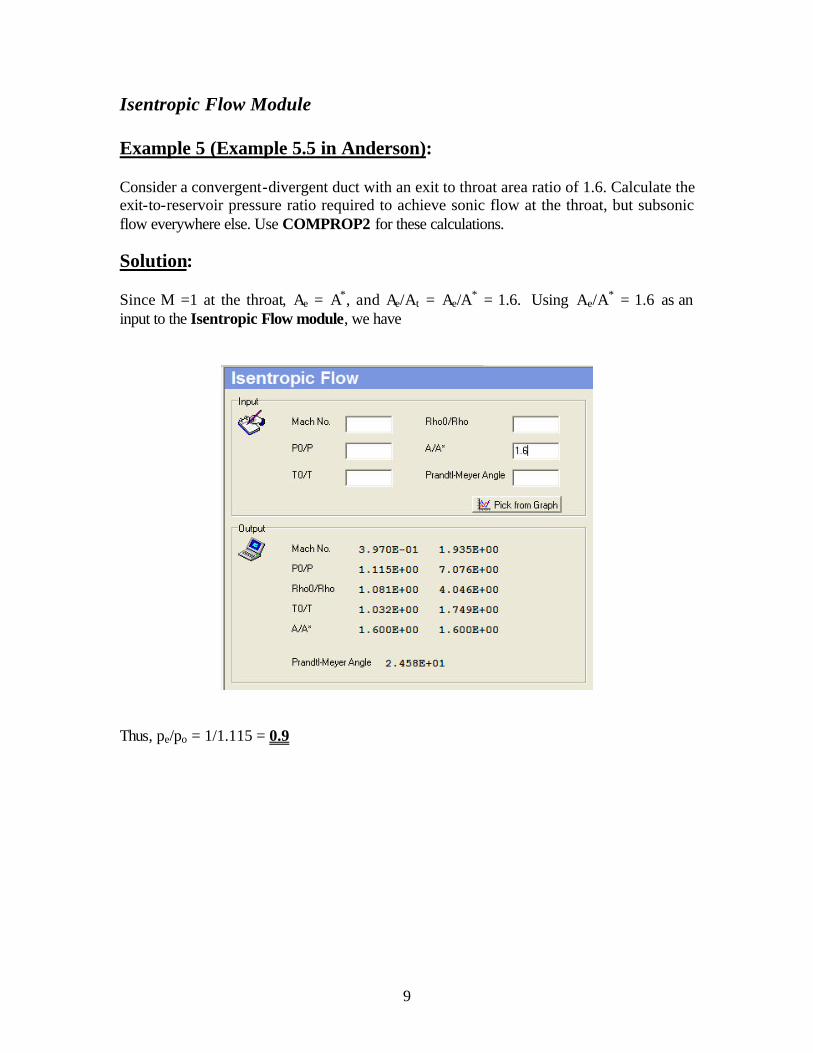
Isentropic Flow Module Example 5 (Example 5.5 in Anderson): Consider a convergent-divergent duct with an exit to throat area ratio of 1.6. Calculate the exit-to-reservoir pressure ratio required to achieve sonic flow at the throat, but subsonic flow everywhere else. Use COMPROP2 for these calculations. Solution: Since M =1 at the throat, Ae = A*, and Ae/At = Ae/A* = 1.6. Using Ae/A* = 1.6 as an input to the Isentropic Flow module, we have

Thus, pe/po = 1/1.115 = 0.9

10

NORMAL SHOCK MODULE

The shock process represents an abrupt change in fluid properties, in which finite variations in pressure, temperature, and density occur over a shock thickness comparable to the mean free path of the gas molecules involved. The supersonic flow adjusts to the presence of the body by means of such shock waves, whereas subsonic flow can adjust by gradual changes in flow properties. Shocks may also occur in the flow of a compressible medium through nozzles or ducts and thus may have a decisive effect on these flows. An understanding of the shock process and its ramifications is essential to a study of compressible flow. For more detail on this topic refer to Chapter 3 of Anderson.

This module is devoted to a consideration of the normal shock wave, a plane

shock normal to the flow direction. This case represents the simplest example of a shock, in that changes in flow properties occur only in the direction of flow; thus, it can be treated with the equations of one-dimensional gas dynamics. The next module will cover the oblique shock wave, positioned at an angle to the flow direction.

To illustrate the use of the Normal Shock module, three selected worked-out

problems from Anderson (3rd edition) have been solved with the assistance of COMPROP2. Please refer to COMPROP2 under “Help, Contents, Module” for the details on this particular module.

Example 1 (Example 3.5 in Anderson): A normal shock wave is standing in the test section of a supersonic wind tunnel. Upstream of the wave, M1 = 3, p1 = 0.5 atm and T1 = 200 K. Find M2, p2, T2 and u2 downstream of the wave with the assistance of COMPROP2. Solution: Using the Normal Shock module, for M1 = 3 as the input, we have

11

Normal Shock Module (Continued) Example 1 (Example 3.5 in Anderson): continued

p2 = (p2/p1)p1 = (10.33)(0.5) = 5.165 atm T2 = (T2/T1)T1 = 2.679(200) = 535.8 K a2 = (γRT2)1/2 = [(1.4)(287)(535.8)]1/2 = 464 m/s u2 = M2a2 = (0.4752)(464) = 220 m/s

12

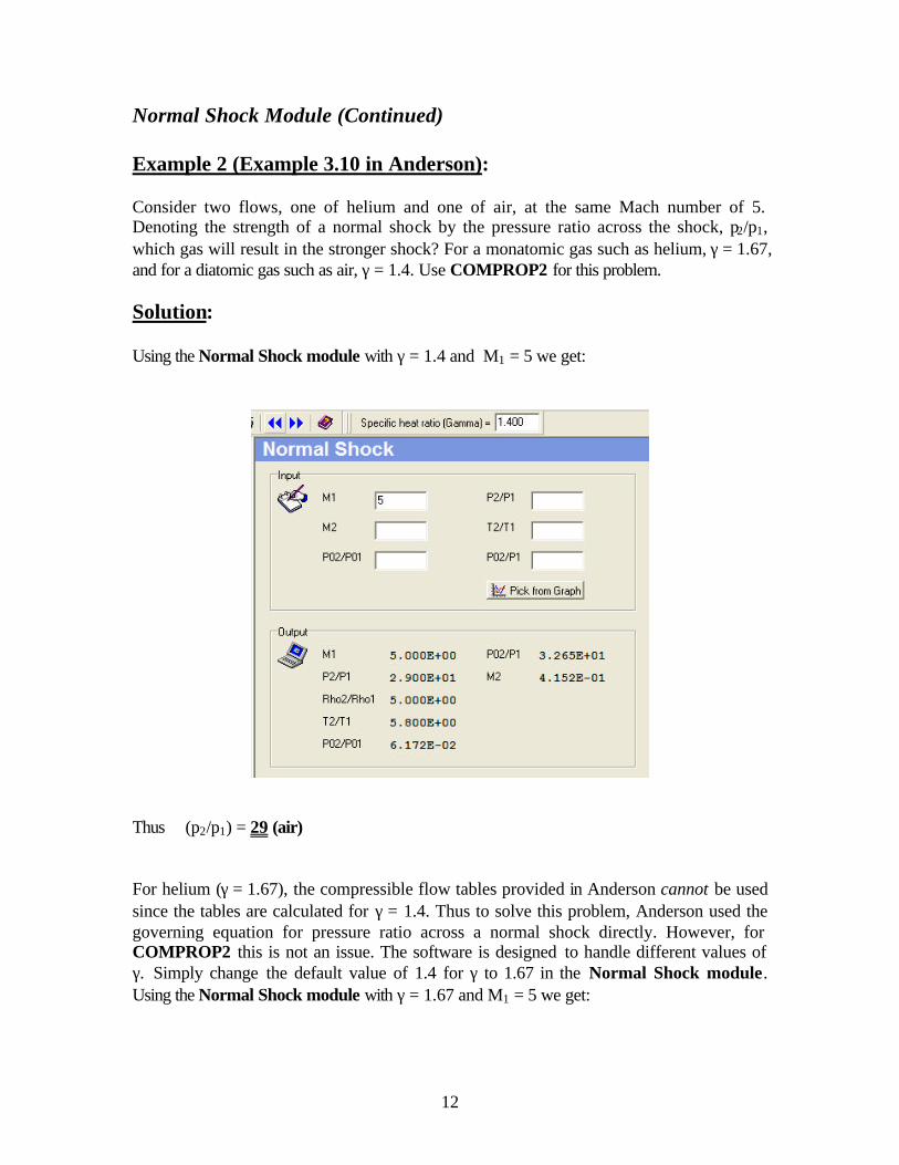
Normal Shock Module (Continued) Example 2 (Example 3.10 in Anderson): Consider two flows, one of helium and one of air, at the same Mach number of 5. Denoting the strength of a normal shock by the pressure ratio across the shock, p2/p1, which gas will result in the stronger shock? For a monatomic gas such as helium, γ = 1.67, and for a diatomic gas such as air, γ = 1.4. Use COMPROP2 for this problem. Solution: Using the Normal Shock module with γ = 1.4 and M1 = 5 we get:

Thus (p2/p1) = 29 (air) For helium (γ = 1.67), the compressible flow tables provided in Anderson cannot be used since the tables are calculated for γ = 1.4. Thus to solve this problem, Anderson used the governing equation for pressure ratio across a normal shock directly. However, for COMPROP2 this is not an issue. The software is designed to handle different values of γ. Simply change the default value of 1.4 for γ to 1.67 in the Normal Shock module. Using the Normal Shock module with γ = 1.67 and M1 = 5 we get:

13

Normal Shock Module (Continued) Example 2 (Example 3.10 in Anderson): continued

Thus (p2/p1) = 31 (helium) Comparing the pressure ratio across the normal shock for air and helium, we conclude that for equal upstream Mach numbers, the shock strength is greater in helium compared to air.

14

Normal Shock Module (Continued) Example 3 (Example 5.6 in Anderson): Consider a convergent-divergent nozzle with an exit to throat area ratio of 3. A normal shock wave is inside the divergent portion at a location where the local area ratio is A/At = 2. Calculate the exit-to-reservoir pressure ratio with the assistance of COMPROP2. Note: The subjects of isentropic flow and normal shock waves were discussed in the prevoius two modules. Many compressible flow systems involve a combination of these two flows. It is instructive at this time to consider one such application to gain an appreciation of some of the interactions that may occur in engineering systems. The particular devise that will be discussed as described in the problem statement given above is the convergent-divergent nozzel. Solution: For this case, we have an isentropic subsonic-supersonic expansion through the part of the nozzle upstream of the normal shock. This part of the problem with be solved using the Isentropic Flow module. Let the subscripts 1 and 2 denote conditions immediately upstream and downstream of the shock, respectively. The local Mach number M1 just ahead of the shock is obtained from the Isentropic Flow module for A1/A1

* = 2.0, namely M1 = 2.2 as shown below.

15

Normal Shock Module (Continued) Example 3 (Example 5.6 in Anderson): continued For M1 = 2.2, use the Normal Shock module to obtain M2 = 0.547 and po2/po1 = 0.6281 as shown below.

For M2 = 0.547 from the Isentropic Flow module, we can find A2/A2

* = 1.26 as shown below. Note that A* is different for 1 and 2 (it changes across the shock wave), but A1 = A2 (the normal shock is assumed to be infinitely thin).

16

Normal Shock Module (Continued) Example 3 (Example 5.6 in Anderson): continued Proceeding with calculation, we have Ae/A2* = (Ae/A2)(A2/A2

*)= (Ae/At)(At/A2)(A2/A2*) = (3)(1/2)(1.26) = 1.89

The flow is subsonic behind the normal shock wave, and hence is subsonic throughout the remainder of the divergent portion downstream of the shock. For Ae/A2

* = 1.89, from the Isentropic Flow module, we have

From the above results we have, Me = 0.32 and poe/pe = 1.076. Since po = po1 and poe = po2, we have pe/po = (pe/poe)(poe/po2)(po2/po1)(po1/po) = (1/1.076)(1)(0.6281)(1) = 0.584

Note: This problem required the use of the Isentropic Flow module and the Normal Shock module.

17

OBLIQUE SHOCK MODULE

The normal shock wave, a compression shock normal to the flow direction, was discussed in the previous module. However, in a wide variety of physical situations, a compression shock wave occurs which is inclined at an angle to the flow. Such a wave is called an oblique shock. An oblique shock wave, either straight or curved, can occur in such varied examples as supersonic flow over a thin airfoil or in supersonic flow through an overexpanded nozzle.

The analysis of the multidimensional oblique shock wave represents a departure

from the one-dimensional flow covered in the previous module, yet in many ways the method of handling the oblique shock parallels that of handling the normal shock. Even though inclined to the flow direction, the oblique shock still represents a sudden, almost discontinuous change in fluid properties, with the shock process itself being adiabatic. This module focuses on the two-dimensional straight oblique shock wave, a type that might occur during the presence of a wedge in a supersonic stream or during a supersonic compression in a corner. For more detail on this topic refer to Chapter 4 of Anderson.

To illustrate the use of the Oblique Shock module, six selected worked-out problems from Anderson (3rd edition) have been solved with the assistance of COMPROP2. Please refer to COMPROP2 under “Help, Contents, Module” for the details on this particular module.

Example 1 (Example 4.1 in Anderson): A uniform supersonic stream with M1 = 3.0, p1 = 1 atm, and T1 = 288 K encounters a compression corner (see Fig. 4.4a of Anderson) which deflects the stream by an angle θ = 20o. Calculate the shock wave angle, and p2, T2, M2, po2, and To2 behind the shock wave with the assistance of COMPROP2. Solution: Using the Oblique Shock module, for M1 = 3.0 and θ = 20o, as shown below, we have Shock wave angle = 37.8 o p2 = (p2/p1)p1 = 3.771(1) = 3.771 atm T2 = (T2/T1)T1 = 1.56(288) = 449.3 K M2 = 1.994

18

Oblique Shock Module (Continued) Example 1 (Example 4.1 in Anderson): continued

From the Isentropic Flow module, for M1 = 3.0, we get: po1/p1 = 36.73 and To1/T1 = 2.8

Hence, from the output of these two modules, we get po2 = (po2/po1)(po1/p1)p1 =( 0.7960)(36.73)(1) = 29.24 atm To2 = To1 = (To1/T1)T1 = (2.8)(288) = 806.4 K

19

Oblique Shock Module (Continued) Example 2 (Example 4.2 in Anderson): In Example 1 (Example 4.1 of Anderson), the deflection angle is increased to θ = 30o. Calculate the pressure and Mach number behind the wave, and compare these results with those of Example 1. Use COMPROP2 for the calculations. Solution: From the Oblique Shock module, for M1 = 3 and θ = 30o, we have

Thus p2 = (p2/p1)p1 = (6.356)(1) = 6.356 atm M2 = 1.41 Note: Compare these results to Example 1. When θ is increased from 20o to 30o, the shock wave becomes stronger, as evidenced by the increased pressure behind the shock (6.356 atm compared to 3.771 atm). The Mach number behind the shock is reduced (1.41 compared to 1.994). Also, as θ is increased, shock wave angle also increases (52o compared to 37.8o).

20

Oblique Shock Module (Continued) Example 3 (Example 4.3 in Anderson): In Example 1 (Example 4.1 of Anderson), the free-stream Mach number is increased to 5. Calculate the pressure and Mach number behind the wave, and compare these results with those of Example 1. Use COMPROP2 for the calculations. Solution: From the Oblique Shock module, for M1 = 5 and θ = 20o, we have

Thus p2 = (p2/p1)p1 = (7.037)(1) = 7.037 atm M2 = 3.02 Note: Compare these results to Example 1. When M1 is increased from 3 to 5, the shock wave becomes stronger, as evidenced by the increased pressure behind the shock (7.037 atm compared to 3.771 atm). The Mach number behind the shock is increased (3.02 compared to 1.994). Also, as M1 is increased, shock wave angle is decreased (29.8o compared to 37.8o).

21

Oblique Shock Module (Continued) Example 4 (Example 4.6 in Anderson): Consider a Mach 4 flow over a compression corner with a deflection angle of 32o. Calculate the oblique shock wave angle for the weak shock case using (a) Fig. 4.8 of Anderson and (b) the β-θ-M equation, Eq. (4.19) in Anderson. Compare the results from the two sets of calculation. Solution: We will solve this problem using COMPROP2. (a) In COMPROP2, we can use the “Pick from Graph” function in the Oblique Shock

module instead of using Fig. 4.8 given in Anderson (Fig. 4.8 of Anderson is similar to the output shown below).

We can directly pick up the desired value of the oblique shock wave angle for the weak shock case for θ = 32o and M1 = 4 from the figure given above. The result is:

β = 48.26o For the conditions selected in the above figure an output can also be generated by COMPROP2. To do this, left-click on the mouse and the generated output is shown below:

22


(b) For this part, using COMPROP2 there is no need to use Eq. (4.19) in Anderson which requires calculation of two additional parameters λ = 11.208 , from Eq. (4.20), and χ = 0.7429, from Eq. (4.21). The user can simply use the interactive part of the Oblique Shock module (third option in the Input menu shown above) with the values of Turning Angle (θ) = 32o and M1 = 4. The result would be identical to Part (a), β = 48.26o.

Note: This problem clearly demonstrates the convenience rendered by COMPROP2 in solving oblique shock problems.

23

Oblique Shock Module (Continued) Example 5 (Example 4.13 in Anderson):

A uniform supersonic stream with M1 = 1.5, p1 = 1700 lb/ft2, and T1 = 460 oR encounters an expansion corner (see Fig. 4.32 of Anderson) which deflects the stream by an angle θ2 = 20o. Calculate M2, p2, T2, po2, To2, and the angles the forward and rearward Mach lines make with respect to the upstream flow direction. Use COMPROP2 for these calculations. Note: This problem deals with Expansion Wave (Prandtl-Meyer Flow). When a supersonic compression takes place at a concave corner (see Fig. 4a of Anderson), the flow is “turned into itself” and an oblique shock occurs at the corner. When supersonic flow passes over a convex corner (see Fig. 4.4b in Anderson), the flow is “turned away from itself” and an expansion wave is formed. An expansion wave emanating from a sharp corner such as sketched in Figs. 4b and 4.32 of Anderson is called Prandtl-Meyer expansion wave. The analysis of Prandtl-Meyer flow requires the relation between the Prandtle-Meyer angle and the Mach number. This relation is either listed as a separate table or is included in the isentropic flow tables. In COMPROP2, the Prandtl-Meyer Angle is part of the Isentropic Flow module. It is instructive at this time to consider two examples of Prandtl-Meyer flow to gain an appreciation of some of the interactions that may occur in engineering systems. For more detail on this topic refer to Chapter 4 of Anderson. Solution: From the Isentropic Flow module, for M1 = 1.5, the Prandtl –Meyer angle (ν1) is 11.91o, as shown below:

24

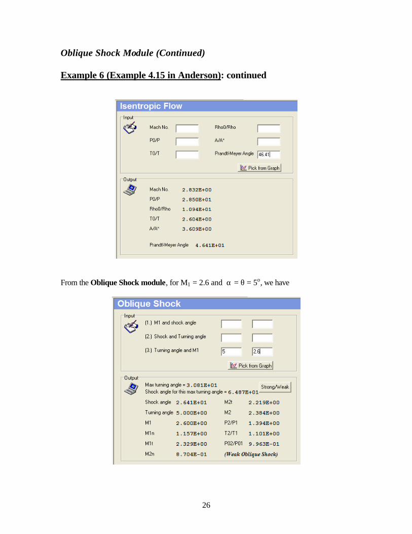
Oblique Shock Module (Continued) Example 5 (Example 4.13 in Anderson): continued So ν2 = ν1 + θ =11.91+20 = 31.91o From the Isentropic Flow module, for ν2 = 31.91o, we have

Therefore M2 = 2.207 p2 = (p2/po2)(po2/po1)(po1/p1)p1 = (1/10.81)(1)(3.671)(1700) = 577.3 lb/ft2 T2 = (T2/To2)(To2/To1)(To1/T1)T1 = (1/1.974)(1)(1.45)(460) = 337.9 oR po2 = po1 = (po1/p1)p1 = (3.671)(1700) = 6241 lb/ft2 To2 = To1 = (To1/T1)T1 = (1.45)(460) = 667 oR Referring to Fig 4.32 of Anderson, the Mach angle (µ), can be obtained from Eq. (4.1) of Anderson which is µ = arcsin (1/M). Thus, µ1 = 41.81o and µ2 = 26.95o. Referring to Fig. 4.32 again, we see that: Angle of forward Mach line = µ1 = 41.81o Angle of rearward Mach line = µ2 – θ2 = 26.95 – 20 = 6.95o

25

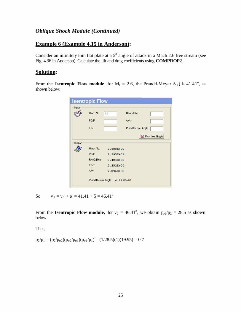
Oblique Shock Module (Continued) Example 6 (Example 4.15 in Anderson): Consider an infinitely thin flat plate at a 5o angle of attack in a Mach 2.6 free stream (see Fig. 4.36 in Anderson). Calculate the lift and drag coefficients using COMPROP2. Solution: From the Isentropic Flow module, for M1 = 2.6, the Prandtl-Meyer (ν1) is 41.41o, as shown below:

So ν2 = ν1 + α = 41.41 + 5 = 46.41o From the Isentropic Flow module, for v2 = 46.41o, we obtain po2/p2 = 28.5 as shown below. Thus, p2/p1 = (p2/po2)(po2/po1)(po1/p1) = (1/28.5)(1)(19.95) = 0.7

26


From the Oblique Shock module, for M1 = 2.6 and α = θ = 5o, we have

27

Oblique Shock Module (Continued) Example 6 (Example 4.15 in Anderson): continued From the Normal Shock module, for M1n = 1.16, we obtain p3/p1 = 1.403 as shown below.

The lift per unit span L ′ is: L ′ = (p3 – p2) c cosα The drag per unit span D′ is: D′ = (p3 – p2) c sinα Recall that the free-stream dynamic pressure is defined as q1= (γ/2) p1

21M

The lift coefficient is then calculated from cl = L ′ /(q1c) = 2/(γ 2

1M )[(p3/p1) – (p2/p1)] cosα = 2/(1.4)(2.6)2(1.403 – 0.7) cos 5o= 0.148 The drag coefficient is then calculated from cd =D′ /(q1c) =2/(γ 2

1M )[(p3/p1) – (p2/p1)]sin2/(1.4)(2.6)2(1.403 – 0.7) sin 5o = 0.013

28

FANNO FLOW MODULE In the Isentropic Flow module, compressible flow in ducts was analyzed for the case in which changes in flow properties were brought about solely by area change. In a real flow situation, however, frictional forces are present and may have a decisive effect on the resultant flow characteristics. The first part of this module is concerned with compressible flow with friction in constant-area, insulated ducts, which eliminate the effects of area change and heat addition. In a practical sense, these restrictions limit the applicability of the resultant analysis; however, certain problems such as flow in short ducts can be handled and, furthermore, an insight is provided into the general effects of friction on a compressible flow. The second part of this module deals with flow with friction in constant-area ducts, in which the fluid temperature is assumed constant. The latter case approximates the flow of a gas through long, uninsulated pipeline. Thus, these two cases cover a wide range of frictional flows and are consequently of great significance. For more detail on this topic refer to Chapter 3 of Anderson.

To illustrate the use of the Fanno Flow module, one selected worked-out problem from Anderson (3rd edition) has been solved with the assistance of COMPROP2. Please refer to COMPROP2 under “Help, Contents, Module” for the details on this particular module. Example 1 (Example 3.17 in Anderson): Consider the flow of air through a pipe of inside diameter = 0.15 m and length = 30 m. The inlet flow conditions are M1 = 0.3, p1 = 1 atm, and T1 = 273K. Assuming f = const. = 0.005, calculate the flow conditions at the exit, M2, p2, T2, and po2 using COMPROP2. Solution: From the Isentropic Flow module, for M1 = 0.3 as an input, we obtain po1/p1 = 1.064 as shown below: Hence, po1 = (po1/p1)p1 = 1.064(1atm) = 1.064 atm

29

Fanno Flow Module (Continued) Example 1 (Example 3.17 in Anderson): continued

From the Fanno Flow module, for M1 = 0.3 and 4f(L1

*/D) = 5.299, we have

30

Fanno Flow Module (Continued) Example 1 (Example 3.17 in Anderson): continued Hence,

2993.115.0

)30)(005.0)(4(299.5

DfL4

DLf4

DLf4 *

1*2 =−=−=

From the Fanno Flow module, 4f(L2

*/D) = 1.2993, we have

Hence, M2 = 0.474 p2 = (p2/p*)(p*/p1)p1 = 2.259(1/3.619)(1atm) = 0.624 atm T2 = (T2/T*)(T*/T1)T1 = 1.148(1/1.179)(273) = 265.8 K po2 = (po2/po

*)(po*/po1)po1 = 1.392(1/2.035)(1.064) = 0.728 atm

Note: The calculated value of p2 in Anderson is in error. A value of 3.619 should haven been used for p1/p* instead of 3.169 used in the text.

31

RAYLEIGH FLOW MODULE We have discussed in Isentropic Flow and Fanno Flow modules the effects on a gas flow of area change and friction. For these cases, flows were assumed to be adiabatic. In this module, the effect of heat addition or loss on a one-dimensional frictionless gas flow in a constant-area duct will be investigated. Flows with heat transfer occur in a variety of situations, for example, combustion chambers, in which the heat addition is supplied internally by a chemical reaction, or heat exchangers, in which heat flow occurs across the system boundaries. For more detail on this topic refer to Chapter 3 of Anderson.

To illustrate the use of the Rayleigh Flow module, one selected worked-out problem from Anderson (3rd edition) has been solved with the assistance of COMPROP2. Please refer to COMPROP2 under “Help, Contents, Module” for the details on this particular module. Example 1 (Example 3.13 in Anderson): Air enters a constant area duct at M1 = 0.2, p1 = 1 atm, and T1 = 273 K. Inside the duct, the heat added per unit mass is q = 1.0 ×106 J/kg. Calculate the flow properties M2, p2, T2, ρ2, To2, and po2 at the exit of the duct with the assistance of the COMPROP2 program. Solution: From the Isentropic Flow module, for M1 = 0.2, we have

32

Rayleigh Flow Module (Continued) Example 1 (Example 3.13 in Anderson): continued Hence, To1 = 1.008T1 = 1.008(273) = 275.2 K po1 = 1.028p1 = 1.028(1atm) = 1.028 atm The specific heat can be evaluate from cp = γR/(γ-1) = (1.4)(287)/0.4 = 1005 J/kg⋅K Now, the exit temperature (To2) can be found from Eq. (3.77) of Anderson To2 = q/cp + To1 = (1.0 × 106/1005) + 275.2 = 1270 K From the Rayleigh Flow model, for M1 = 0.2, we have

Hence, To2/To

* = (To2/To1)(To1/To*) = (1270/275.2)(0.1736) = 0.8013

33

Rayleigh Flow Module (Continued) Example 1 (Example 3.13 in Anderson): continued From the Rayleigh Flow module, for To2/To

* = 0.8013, we have M2 = 0.58, as shown below

From the Rayleigh Flow module, for M2 = 0.58, we have

34

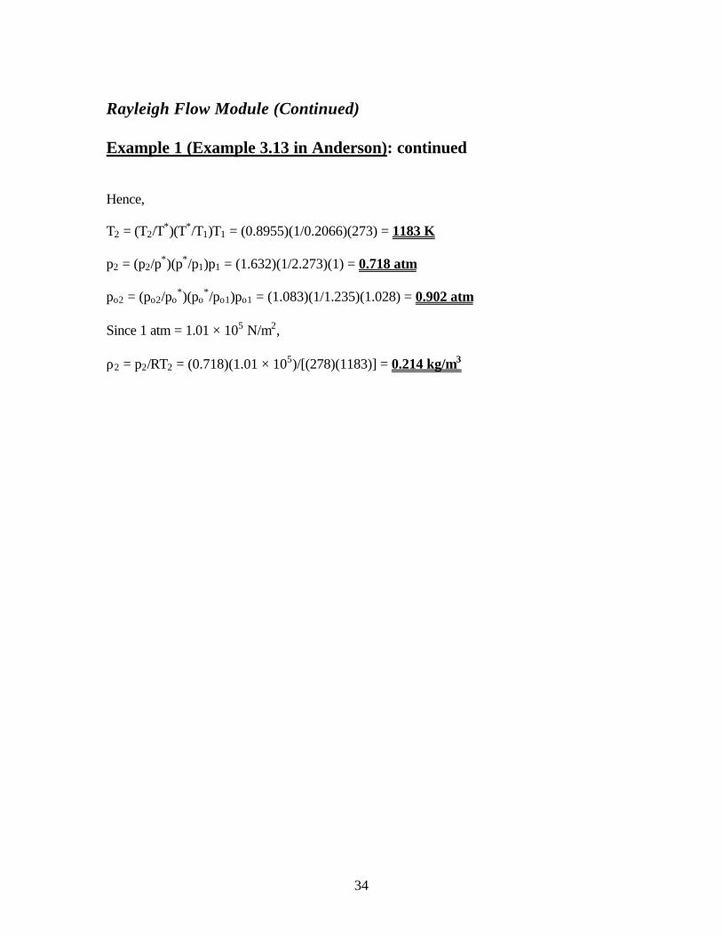
Rayleigh Flow Module (Continued) Example 1 (Example 3.13 in Anderson): continued Hence, T2 = (T2/T*)(T*/T1)T1 = (0.8955)(1/0.2066)(273) = 1183 K p2 = (p2/p*)(p*/p1)p1 = (1.632)(1/2.273)(1) = 0.718 atm po2 = (po2/po

*)(po*/po1)po1 = (1.083)(1/1.235)(1.028) = 0.902 atm

Since 1 atm = 1.01 × 105 N/m2, ρ2 = p2/RT2 = (0.718)(1.01 × 105)/[(278)(1183)] = 0.214 kg/m3

35

AIRFOIL MODULE

The design of an airfoil should be such as to provide a lift force normal to the undisturbed flow accompanied by low drag force in the direction of the undisturbed flow. The shape of a wing section to be used in low-speed, incompressible flow is the well-known teardrop or streamlined profile. In supersonic flow, however, the design must be completely modified owing to the occurrence of shocks. The high pressures after the shock wave produce excessive drag forces on the airfoil. To minimize wave drag, or drag due to the presence of shocks, the supersonic airfoil must have a pointed nose and also be as thin as possible. The ideal case is a flat plate airfoil, possessing zero thickness. For more detail on this topic refer to Chapter 4 of Anderson.

To illustrate the use of the Airfoil module in the analysis and design of supersonic airfoils, an example problem has been solved with the assistance of COMPROP2. Please refer to COMPROP2 under “Help, Contents, Module” for the details on this particular module.

Example 1 (Supersonic Airfoil Analysis): Consider the supersonic airfoil shown below and calculate the lift and drag forces by two methods: (a) hand calculation with the assistance of different COMPROP2 modules and (b) use of the Airfoil module alone in the COMPROP2 program. Given:

Where: Angle of attack = 3o

Mach no.ahead of airfoil = 2.6 Pressure ahead of airfoil = 40 kPa

36

Airfoil Module (Continued) Example 1 (Supersonic Airfoil Analysis): continued

The angle of turn for various waves is summarized below

Type of wave Angle of turn Shock Wave (A, from 1 to 2) 5° Expansion Wave (B, from1 to 3) 1° Expansion Wave (C, from 2 to 4) 4.67° Expansion Wave (D, from 3 to 5) 4.67°

Solution: Part (a): For oblique shock wave A, M1 = 2.6 and the turning angle = 5o, from the Oblique Shock module, we have

For expansion wave B, from the Isentropic Flow module, for M1 = 2.6, we have

37


Since the flow is turned through 1o by the expansion wave, the new angle (Prandtl-Meyer angle) is now 42.41o, using the Isentropic Flow module again, we have

Hence, p3 = (p3/po3)(po1/p1)p1 = (1/21.38)(19.95) (40) = 37.32 kPa

38

Airfoil Module (Continued) Example 1 (Supersonic Airfoil Analysis): continued Now consider the expansion wave C with Mach number ahead (M2 = 2.38, obtained from the Oblique Shock module), from the Isentropic Flow module we have

Since the flow is turned by the expansion wave through 4.67o, the new angle (Prandtl-Meyer angle) is now 36.26o + 4.67o = 40.93o, with this angle as the new input to the Isentropic Flow module, we have:

39

Airfoil Module (Continued) Example 1 (Supersonic Airfoil Analysis): continued Hence, p4 = (p4/po4)(po2/p2)p2 = (14.17)(1/19.3)(56.1) = 41.19 kPa [Note: p2 is from p2/p1 = 1.403 (the Normal Shock module), p2 = (1.403)(40) = 56.1 kPa] For expansion wave D, with M3 = 2.64, from Isentropic Flow module we have

Now the expansion angle (Prandtl-Meyer angle) should be 42.31o + 4.67o = 46.98o and this angle is now the new input to the Isentropic Flow module.

40


Then, p5 = (p5/po5)(po3/p3)p3 = (1/29.73)(21.23)(37.27) = 26.61kPa Therefore, p2 = 56.1 kPa, p3 = 37.32 kPa, p4 = 41.19 kPa, and p5 = 26.61 kPa. For the areas, A2 = A3 = 0.4/cos 2° = 0.4 m2 A4 = A5 = 0.3/cos 2.67° = 0.3 m2 The lift force per meter span is then Lift Force = 56.1 × 0.4 × cos 5° – 37.32 × 0.4 × cos 1° + 41.19 × 0.3 × cos 0.33°

– 26.61 × 0.3 × cos 5.67° = 11.84 kN/m span The drag force per meter span is then Drag Force = 56.1 × 0.4 × sin 5° – 37.32 × 0.4 × sin 1° + 41.19 × 0.3 × sin 0.33°

– 26.61 × 0.3 × sin 5.67° = 0.978 kN/m span

41

Airfoil Module (Continued) Example 1 (Supersonic Airfoil Analysis): continued Part (b): Now, let’s consider the usage of the Airfoil module to calculate the lift and drag forces for the problem that was solved in Part(a). Select the module by clicking the icon and input the airfoil chord length which is 0.7m, the Mach number ahead of the airfoil which is 2.6, the pressure ahead of the airfoil which is 40 kPa, and finally the angle of attack which is 3o. Since the length of the airfoil is 0.7m, with the other specifications, user can easily draw the airfoil in the CAD environment provided by the module.

Click the calculation icon, then you can get the lift and the drag force!

42


The lift force from the output is 11.63 kN/m span and the drag force is 0.97 kN/m span. Comparing to Part (a) of the example problem both results are almost identical. The user can also conduct parametric studies for design purposes by varying the angle of attack, the pressure ahead of the airfoil, or even the shape of the airfoil. For example, the angle of attack is now changed to 15o

43

Airfoil Module (Continued) Example 1 (Supersonic Airfoil Analysis): continued The lift force changes from 11.65 to 60.21 kN/m. If the user wants to change the shape of the foil, all one needs to do is to drag the red and blue dots. This is shown below.

In this case, it can be observed that the lift force is slightly larger (63.27 kN/m compared to 60.21 kN/m); however, the drag force has increased significantly (26.43 kN/m compared to 16.58 kN/m). Note: This example problem demonstrated how the different modules in COMPROP2 could be used for analysis/design of the Supersonic Airfoil. It was also demonstrated that the special module called Airfoil module is much easier to use for this type of problem. In addition, this module offers tremendous opportunity for in depth analysis and design of supersonic airfoils.

user guide for comprop2 -...

Documents