use of the r-x diagram in relay work

Use of the R-X Diagram in Relay Work

GET-2230B

TABLE OF CONTENTS

Introduction

Ohmic Elements on the R-X Diagram

Ohmic Relay Characteristics on the R-XDiagram

System Conditions on the R-X Diagram

Combined System and Relay Characteristics onthe R-X Diagram

Out-of-step Blocking

Out-of-step Tripping

Loss-of-excitation Characteristics

Appendix A 24

Per-unit Notation 24

Conclusion 25

References 25

Page

3

3

5

8

15

19

Copyright 1966 by The General Electric Company

Switchgear Department

Philadelphia, Pa.

THE USE OF THE R-X DIAGRAM IN RELAY WORK

INTRODUCTIONPractical system economics demand heavier line

loadings than were considered possible years ago.These increased loadings have focused attention onsystem stability and its horde of associated prob-lems. The consequent emphasis on circuit relia-bility means that more and more dependence mustbe placed on the system relaying. Because of thisincreased dependence, we demand increased exact-ness in performance. Simple relays, actuated by asingle operating quantity, are found lacking whenmeasured by these newer performance require-ments. Thus, we have turned more and more torelays actuated by multiple operating quantities.For instance, we find that simple overcurrent re-lays are forced to yield more and more of the sys-tem relaying responsibility to some form of ohmicrelaying; that is, relaying actuated by three elec-trical quantities : voltage, current and phase angle.Our older relay application techniques based onthe overcurrent concept are gradually being re-placed by newer techniques based on the complexrelationship between voltage and current. The ap-plication tool for these ohmic relays is the R-X dia-gram. Before we examine this tool, however, abrief review of relay requirements and relay char-acteristics is highly desirable.

For the sake of simplicity and brevity, we willconfine this discussion to line relays and balancedthree-phase conditions.

The line relay has the primary responsibility ofclosing the line circuit-breaker trip circuitpromptly for any fault within the limits of the line.As we all know, this part of its job is simplicityitself when compared to its responsibility for nottripping unless a fault actually exists and lies be-tween the line terminals. ‘This latter part of thetask is the part that is responsible for nearly all ofthe grey hairs in any relay department.

As an illustration, let us suppose that we weregiven the task of writing the major command-ments for an ideal relay. We would find that theywould fall naturally in two groups as follows:“Thou Shalt-”

1.

2.

Thou shalt trip all faults within thy zone ofprotection irrespective of changes in gener-ation.Thou shalt trip these faults at highest speed ;yea, thou shalt make thy tripping decisionsin terms of a second split into a hundredparts.

“Thou Shalt Not-”1. Thou shalt not trip faults outside thy zone of

protection except in back-up assistance to afailing brother.

2. Thou shalt not trip under heavy load condi-tions even though thy coils do carry muchcurrent.

3. Thou shalt not trip during power swings,denying always the tempting surges of cur-rent and voltage.

It is easy to see why any relay would have diffi-culty in keeping these commandments. As a mat-ter of fact, these requirements have eliminated theover-current relay on important lines. The severerequirements of these. commandments have thusforced the development and utilization of theohmic relays.

OHMIC ELEMENTS ON THE R-X DIAGRAMWhat is an ohmic relay? We have broadly justi-

fied the name, “ohmic,” by the statement that theserelays operate in response to the three variables:voltage, current and phase angle. In order toappreciate this name, and in order to understandthe operation of these relays we must consider thevarious relay elements individnally.

In general, these elements respond to at leastthree of the four familiar torque-producing com-ponents :

1.

2.

3.

4.

Voltage Component (Torque proportional toE2)Current Component (Torque proportional to12)Product Component [Torque proportional toExIxf(B)]Control Spring Torque

Thus, we can write a general torque equation foran ohmic element :

Torque = tK,E” *K,12 +K, EI f (r,e) aK,The conventions which we have adopted for thisequation are :(a) contact-closing torque is positive; (b) K1, KZ,KS are independent design constants which may beused with either sign and varied in magnitude tomeet requirements ; (c) K, represents the springtorque, assumed to be constant ; (d) y is the designangle of maximum torque ; (e) E, I, and 0 are thefamiliar operating quantities supplied to the relay.(7 and 6 are angles by which I lags E.)

As the first example of the use of this equation,we will select K1 = K2 = 0, Kq negligible, K3 posi-tive and f (~~0) = sin (90” + y - 0). The equationnow reads : T = + K3 EI sin (150” - 0) for a relaywhere y = 60°. This is recognizable as a direc-tional element, wherein positive, contact-closing,torque is realized for values of 0 between 330° and150°, with maximum positive torque at 0 = 60°.

For our second example, we will choose K1 = 0,Kq negligible, K, positive, f (y&3) = sin 0, and use

3

GET-2230B The Use of the R-X Diagram in Relay Work

the minus sign for Ka. Our equation becomes : T =+ K,12 - K,EI sin 0. In order to analyze this equa-tion quickly, we will substitute (E/I) sin 0 = X,thusly ; T = + K,I” - K,I’X. This is the equationfor a reactance element which will operate to closeits contacts whenever X drops below a value deter-mined by the proportion of K2 to K3.

The next example will be the impedance elementwherein we, as designers, will select K, as nega-tive, K, positive, K8 as zero and K, as negligible.Our equation: T = -K,E2 + KJ2. Once again wewill substitute for ready analysis another relation-ship, E/I = Z. Rearranging the above equation:T = +KJ2 - K,12Z2. Thus the element will oper-ate to close its contacts whenever Z drops below avalue determined by K2 and K1.

The last element we will spend time to discussmight be called a directional element with voltagerestraint. Selecting K, = 0, K, negligible, a minussign for K1 and f(y,B) = sin (90° + y - 8), withKs positive, we have an equation T = +K3EI sin(90° + y - 0) - KIE”. If we use the relationshipE/I = Z to simplify this equation we find: T =K,PZ sin (90° + y - 0) - K,12Z2. This relay willoperate whenever K,Z2 is less than KaZ sin (90” +u--e).

This is very interesting as far as we’ve gone, buthow do we evaluate these operating characteris-tics ? Let’s examine the last element described by

T = K,EI sin (90° + y - 0) - K1E2. Pos i t ive ,contact-closing torque will be realized wheneverK3EI sin (90° + y - 0) exceed K,E2; negative, orcontact-opening, torque will be realized wheneverthe reverse is true. The boundary of relay opera-tion is thus defined by T = 0, i.e., when operating(positive) torque equals restraint (negative)torque. With this in mind, we can plot I sin (150°- 0) = (K1/K3) E (for y = 60°) for a single, defi-nite value of voltage, E = E,, as shown in Fig. la.If we select other values of voltage, we must drawnew curves as shown on Fig. lb for E = 0.5E,,l.OE,, 2.OE,. Thus we have arrived at an I vs 9plot of this element’s operating characteristic,using E, as a parameter.

Again, we are tempted to say that this is veryinteresting, but how can we apply such a relaysince the relay voltage will be different for differ-ent system faults and, more confusing, since it willbe different for the same fault under differentsystem conditions ?

The answer to this question will be found in theR-X diagram. The value of the R-X diagram lies inthe two facts :

1. Ohmic relay characteristics can be simplyshown. This is true because these character-istics may be plotted in terms of only twovariables, R and X (or Z and 0), rather thanthe three variables, E, I and 0.

Fig. 1a. Operating Characteristic

El S in (150 - 6) = -$ E2

E = Constant(60” MHO Element)

Fig. 1b. Operating Characteristic

El Sin (150 - 0) = 2 E2

E = 0.5 E,, 1.0 Es, & 2.0 Es(60° MHO Element)

I_ The Use of the R-X Diagram in Relay Work GET-2230B

NOTE :OPERATING AREA SHOWN SHADED

-X

Fig. 2. Operating Characteristic

Z= 2 Sin (150 - B)

(60° MHO Element)

2. System conditions affecting the operation ofthese relays can be shown on the same dia-gram. These points will be covered sepa-rately and then considered together.

I NOTE :-X OPERATING AREA SHOWN SHAOED

Fig. 3. Operating Characteristic-

(Impedance Element)

to negative net torque. The mathematical treat-ment of these relay elements is therefore similar.The directional element is an exception as shownby the equation: T = +K,EI sin (150° - 0).From this equation, we see that a torque is devel-oped for all values of E and I except for two valuesof 0: 150° and 330°. The sign of this torque will bepositive for values of 0 from 330” to 0° to 150°and negative for values of B from 150° to 270° to330°. Maximum torques will be developed at 60°

OHMIC RELAY CHARACTERISTICSON THE R-X DIAGRAM

Consider again the equation used for Fig. 1: Isin (150° - 0) = (K1/K3) E. If we recognize thefact that the impedance to a fault from the relaylocation is shown to the relay by the relationshipE/I = Z, this equation becomes (K,/K1) sin (150°- 0) = Z. This equation defines the operatingpoint of the relay in terms of Z and may be plottedon an R-X diagram as shown in Fig. 2. Positivecontact-closing torque will be realized whenever(K,/K1) sin (150° - 0) is greater than Z, that is,whenever the fault impedance falls inside the cir-cle. This simple plot does not depend on any param-eters of operating quantities but defines the oper-ating characteristic for all values of E, I and 0.This is the characteristic of the mho element usedin the GCY relay.

In a similar manner, we can simplify the equa-tions for the impedance element, plotted in Fig. 3,and the reactance element, plotted in Fig. 4. Allvalues of fault impedance which will cause therelay to close its contacts lie in the shaded areas ofthese curves. It will be observed that the elementsof Fig. 3 and 4 operate similarly to that of Fig. 2,in that a restraint torque and an operating torquejust balance at the changeover point from positive

+X

Fig. 4. Operating CharacteristicX=5

KX(Rcoctance Ncmcnt)

5


(positive torque) and 240” (negative torque).Thus, the operating line of the relay may be drawnas shown on Fig. 5 if the control spring is ne-glected. It should be noted that the directionalelement is not an ohmic element in the usual sense,although its characteristic may be convenientlyshown on an R-X diagram.

Another useful characteristic is found in the“offset mho” element. This element is similar tothe mho element but has a portion of the operatingcurrent introduced in the voltages of the equation.Changing the fraction of the operating currentthus used will change the offset as shown in Fig. 6.(In the practical relay, this offset is determined bytaps.)

This completes the list of ohmic elements whichwill be described, although there are many otherinteresting and useful variations of the principlescovered above. Our next concern is the combina-tion of these elements to form a distance relay.This discussion will be confined to three types ofdistance relays and a brief review of out-of-stepblocking. All three of the distance relays will beassumed to have an ideal time-distance character-istic as shown in Fig. 7. The 1st zone gives instan-taneous operation while the 2nd and 3rd zones com-plete the trip circuit only through the contacts ofa timer to give time delay tripping as shown.

(1) The Impedance Relay is composed of threeimpedance elements, each adjusted for a different

/ -X

Fig. 5.

NOTE :POSlTlVE TORGUE

tX’:R&T;NG AREA SHOWN

Operating CharacferisficT= +K, El Sin (150-0)

(Directional Element)

MHO ELEMENTWITH NO OFFSE

Fig. 6. Operating Characteristicsof MHO Element

And of Offset MHO Element

STATION STATION STATION STATIONi 2 3 4

I i

I- DISTANCE --Fig. 7. lllustration of Time-Distance Plot

For Ideal Single Circuit Lint ShownRelay Location: Station 1

ohmic reach. The directional element controls thetripping circuits for all three elements thus pre-venting relay operation for faults in the backwardsdirection. The characteristics of this relay areshown in Fig. 8.

(2) The Reactance Relay is composed of a re-actance element, which gives 1st and 2nd zone pro-tection, and a mho element which doubles as thestarting unit and the 3rd zone protection element.

6

The Use of the R-X Diagram in Relay Work GET-2230B

DIRECTIONAL ELEMENT

-XlFig. 8. Three-step Impedance Relay

Characteristic(For Line of Fig. 7)

The contacts of the starting mho element and thereactance element are in series so that relay trip-ping is confined to those areas within the bounda-ries shown by the solid lines of Fig. 9. This pre-vents relay operation for faultsdirection or on load currents.

in the reverse

_ __-____---_ _-_____

-R +R

-XI

Fig. 9. Three-step Reactance TypeRelay Characteristic

(For Line of Fig. 7)

3RD ZONE- -

2ND ZONE

IST ZONE

- X l

Fig. 10a. Three-step MHO RelayChorocteristic(For Line of Fig. 7)

No Offset

(3) The Mho Relay is composed of three mhoelements, each adjusted for a different reach. Itwill be seen that there is no need for a “limiting”element such as required in the other two relays,since the mho element closely approaches the idealrelay element. In the practical relay, the 3rd zoneelement may be used as shown in Fig. l0a, or withreversed 3rd zone as shown in Fig. l0b. In eithercase, the 3rd zone may be offset to some extent,depending upon the application requirements.

Out-of-step blocking relays, in general, utilizeone of two basic elements: (1) an impedance ele-ment; (2) the mho element. Examples of these

2ND ZONE4

\ REVERSED

r--3RD ZONEOF STA. 2

_ REVERSED3RD ZONE

/ //+R

/ DOTTED CHARACTERISTICSHOWS BACK-UP PROTECTION OF

-X LINE 2-3 BY REVERSED 3RDZONE OF RELAY Al STATION2 NORMALLY LOOKING TOWARDSSTATION I.

Fig. 10b. Three-step MHO RelayChorocteristic(For Line of Fig. 7)

Showing Reversed 3rd Zone

7


Fig. 11a. Out-of-step Blocking of ImpedanceRelay Using an Impedance Element

relay characteristics are shown in Fig. l1a and llb.Further discussion of this function will be givenlater.

In the foregoing discussion, there were a num-ber of instances wherein interesting and pertinent

Fig. 11b. Out-of-step Blocking of MHORelay Using an Offset MHO Element

8 ’

STATION STATION STATION STATION STATION1 2 3 4 5

1 +j2.0 ~6.+,3.76 1 1.63+j4.55 1 1.1+j2.82 1 1.0+j2.7 k]Ifj

SYSTEM SECONOARY IMPEDANCES IN OHMS

t+-33-t37~33+3SM

APPROXIMATE LINE MILEAGE

* THESE LENGTHS ON DRAWING INOICATE EQUIVALENTSYSTEMS IMPEDANCE AT A 8 B.

Fig. 12. One Line Diagram of System Used in Examples(Single Circuit Line)

questions were avoided; foremost among thesewould be the question, “Why show these charac-teristics on the R-X diagram?” We have seen thatit is convenient to do so from the viewpoint of plot-ting their operation in simple curves, but that isscant justification until we consider how varioussystem conditions appear on the same plot. Thiswill then be the next step in our discussion.

SYSTEM CONDITIONS ON THE R-X DIAGRAM

In order to use the diagram, we must begin withan equivalent two-machine system. The imped-ances used may thus represent combined systemson either end of the line we are studying. In ourcase we will assume a system reduced to the caseof Fig. 12. Here the system ohms have beenchanged to “secondary ohms.” We can now plotthe system impedance on a “secondary-ohms” im-pedance diagram, as shown in Fig. 13, by the fol-lowing steps: Starting at Gen. A, the secondaryimpedance to an imaginary fault at Station 1 is(0 + j 2.0) ohms. The + j 2.0 is plotted along theX axis in the positive direction (Fig. 13a). If wemove our imaginary fault to Station 2, the second-ary impedance is now (0 + j 2.0) + (0.94 +j 2.76) = (0.94 + j 4.76) ohms (Fig. 13b). We cancontinue in this manner until we reach the end ofthe system, i.e., back of the reactance of the equiv-alent generator at B (Fig. 13c). Our equivalentsystem impedance total is then (4.67 + j 15.23)ohms. The resulting R-X diagram of the system,the “system impedance line” and the “system im-pedance center’* are shown in Fig. 13d.

We should pause here briefly to review and em-phasize some of the conventions we have automat-ically adopted.1st. The units of R and X are to the same scale,

e.g., one ohm resistance equals one horizontalscale unit, one ohm reactance equals one verti-cal scale unit.


+x

I

+i2I-R A +R

-x

Fig. 13a. Fault at Station

I as Seen from A

+xl+2

I++ j 4.76

b- R +R

Fig. 13b. Fault at Station

2 as Seen from A

5

I4+

I3+

i

2+

1 +j15.83

-XI

I

-R A +R

:I+4.67

- x

+B

Fig. 13c. Fault at Station B as Seen from A(Other Stations as located Previously)

IWPEOANCE CENTEROF sY6lEM

SYSTEM IMPEDANCELINE

+

-I

+6I+S

.L/

f’3;:

+R

Fig. 13d. R-X Diagram of System Showing-x I

System Impedance line and Impedance Fig. 13e. large load of Station 1Center of System Single End Feed from Station A

Fig. 13. Construction of the R-X Diagram for the System of Fig. 72

2nd. We have adopted a sign convention of plus Rto the right and plus X to the top, as seenlooking towards Station B. The importance ofthis sign convention will be realized when wetemporarily place a large load of laggingpower factor, say at Station 1 with Station Bdisconnected. In this case we would see alarge +R and a smaller +X from Station A(Refer to Fig. 13e). (The value plotted rep-resents a load of approximately 33,000 kva,just twice normal circuit loading for thisline.)

3rd. The sign conventions hold only when we“look” in the same direction as we did when weplotted the diagram. That is, a fault at Sta-tion 4 (or a lagging power-factor load atStation 4) when viewed from Station B, obvi-ously must appear as +R and +X. Strictlyspeaking, a new R-X diagram should beplotted for this condition, but the mental gym-nastics involved are of little difficulty whencompared with the advantages of using thesame diagram for both directions in this sim-ple case.

9

GET-22306 The Use of the R-X Diagram in Relay Work

\ I / I

Fig. 14. Constant Voltage Ratio Circlesfor System of Fig. 12

4th. The location of the origin was assumed to beback of the generator reactance at A. Thislocation is convenient for load transfers andpower swings between stations when viewedfrom A. It is not so convenient when consider-ing relay operations at the intermediate sta-tions. Fortunately, we can avoid the incon-venience of subtracting the vector impedancebetween Station A and the intermediate sta-tion by locating the origin at the relay loca-tion. This will enable us to measure directlythe impedance seen by that relay for varioussystem conditions.

We are now ready to investigate various systemphenomena, as interpreted by the R-X diagram,

One of the earliest attempts at determiningqualitative relay performance data during swingconditions resulted in the development of a newconcept of system and relay performance. C. R.Mason presented an AIEE paper(l) in 1937 inwhich he analyzed relay performance during swing

Fig. 15. Constant Angular SeparationCharacteristics for System of Fig. 12

conditions. The results of his analysis were sum-marized in plots of relay torque as a function ofthe separation angle between the two machines ofhis equivalent system. At the same time Mr. J. H.Neher presented the first papert2) on distance-relaycharacteristics plotted on an impedance diagram,and later gave Mason valuable suggestions in adiscussion of Mason’s paper(l). Neher pointed outthat, for equal voltages back of machine reactances(EA/EB = 1.0), the apparent system impedancevaried (as the two machines slipped a pole withrespect to each other) along a line which was theperpendicular bisector of the system impedanceline, In the closing discussion of his paper(l),Mason then showed this “swing line” on the sameR-X diagram with different relay characteristics,This ‘was indeed a true pioneering step, for it of-fered a readily understandable analysis of a prob-lem that was becoming increasingly acute.

Subsequent authors(3s4) have enlarged and ad-vanced this concept beyond the limitations of this

(1,2,3*4)For numbered references, see list at end of paper.

1 0

The Use of the R-X Diagram in Relay Work GET-22306

Fig. 16. General Per-unit ImpedanceDiagram

particular case and developed curves for variousratios of EA/EB. In this work it was proved thatthe apparent impedance during out-of-step condi-tions followed a definite circle for each value ofEA/EB. These circles were all centered on thesystem impedance line with radii and off sets deter-mined by the various values of this voltage ratio.These characteristic circles are shown on Fig. 14.Note that the specific case of EA/EB = 1.0 is buta logical limit to the increasing circular character-istics (the radius and offset for this case are eachinfinite). NOTE : Certain simplifying assumptionshave been made for this discussion. The most im-portant of these are: (1) the system can be rep-resented by a single circuit between Station A andStation B ; (2) the effective excitation voltage re-mains constant; (3) the machine impedances re-main constant.

The mathematics and curves for the generalizedcase have been summarized and presented in apaper by Miss Edith Clarkec4). In this paper MissClarke presents another series of curves wellworth our attention. This series concerns thosecircles of equal angular separation. If the angularseparation of the two machines is held constantwhile the voltage ratio is varied, the apparent im-

t4)For numbered references, see list at end ofpaper.

pedance will trace a portion of a circle whichpasses through both A and B and whose center lieson the perpendicular bisector of the system imped-ance line. The radii and offsets of these circles aredetermined by the angular separation between Aand B. These circles are shown on Fig. 15. Thesecircles have a peculiarity that should be noted.The line A-B is a portion of the circle (having in-finite radius) which represents 0 and 180 degreesseparation, and it also separates the right and leftportions of each constant angular separation circleinto two characteristics, wherein the separationangle for the two parts differs by 180 degrees.Thus, the 90-degree separation circle on the rightbecomes the 270-degree separation circle on theleft.

The foregoing comments will become clearer ifwe consider the general per-unit diagramc4), Fig.16, the use of which greatly reduces the time ofcalculation, as illustrated in a discussion of MissClarke’s paper(“). In using this diagram, it is nec-essary to shift the vertical axis to coincide withthe impedance angle of the system. A detailed dis-cussion of this diagram and its use is not in order;however, it will be helpful to trace two cases on thediagram. In the first instance, assume EA/EB =1.0. Thus, our swing characteristic is the horizon-tal line. Suppose we start our swing when A leadsB by 25 degrees, we would then trace a path: a-

l l


-x IFig. 17. Working Example for System

of Fig. 12EAShowing: - = 1 .O Swing LineEBI#. = W, 120’ Separation CurvesPoint P for a 27,000 Kw Load FlowRelay Zone Reaches

25°, bŽ45”, c-90”, d-180”, e-330”. It will behelpful to trace another path, say for EA/EB =0.5. At zero degrees separation, machine A “sees”what is predominantly -X (point f of Fig. 16) orcapacitive reactance. This will jibe with operatingexperience when we consider that this appears asa highly inductive load to machine B. Once againn-e can trace points around this circle for variousangles : g-25”, h-45”, k-90”, m-180”, n-340”. Before we dismiss this diagram, we shouldnote the 90-degree separation circle. This circle iscentered at the system impedance center andpasses through both A and B. For any value ofEA/EB, the apparent impedance of the systemmust pass through this circle as the separationangle reaches and passes 90 degrees. This circle,for 90-degree separation, is an important one forus to remember for two reasons : (1) It is easy toconstruct, and (2) it indicates an approximate limit,in angular separation, for power swings of the sys-tem if steady-state stability limits are not to beexceeded.

This limited discussion has indicated that theR-X diagram is a useful tool in describing and ana-lyzing various system conditions. We have seen, inthe previous discussion, that it is useful in study-ing relay characteristics. Our next step is thus thecombination of the relay characteristic and systemcharacteristic on one diagram.12

Fig. 18. Impedance Relay Superimposedon Working Example (Fig. 17)

COMBINED SYSTEM AND RELAYCHARACTERISTICS ON AN R-X DIAGRAM

Refer to Fig. 17. This is the R-X diagram ofour system of Fig. 12 with several referencessuperimposed thereon. The EA/EB = 1.0 powerswing line is shown, as are the 90”- and 120”-separation circular arcs. In addition, we now havea point P indicating the impedance seen for aninterchange loading of aproximately 27,000 kw.Note that the origin has been shifted to Station 2of Fig. 12. We will consider various distance re-lays for the line between Stations 2 and 3, eachhaving lst, 2nd, 3rd zone reaches as indicated onour working example, Fig. 17.

The impedance relay characteristic for this caseis shown, superimposed on the working example,in Fig. 18. The directional unit is necessary to pre-vent relay tripping for faults between Station 2and Gen. A.

Notice that third zone tripping will occur forany separation beyond 90 deg (EA/EB = 1.0) andfor even less angular separation than 90 deg ifEA/EB < 1.0. Furthermore, at certain values ofEA/EB, the 1st zone instantaneous trip area ex-tends into the 120-degree separation area. Since120” separation is an approximate transient stabil-ity limit for most systems of this pattern, someform of blocking for power swings is almost man-


Fig. 19. Reactance Relay (Type GCX)Superimposed on Working Example (Fig. 17)

datory. If we attempt to provide out-of-stepblocking for the complete relay, we find that ourblocking impedance element would come into theload area (see Fig. lla) . This, of course, is intoler-able if we expect to carry appreciable load overthis line since our line relays would be continuouslyblocked during heavy load transfer periods.

The Reactance Relay with mho starting ele-ment is shown superimposed on the working ex-ample in Fig. 19. Again, a glance will show theneed for the limitation the starting unit character-istic imposes upon the reactance element. Forexample, load flow towards B, for all practical volt-age ratios (EA/EB), will fall in the operatingrange of the reactance element. The tripping rangeof the relay is limited by the starting unit charac-teristic so that the relay tripping area is far re-moved from even the heaviest load areas. It isinteresting to note that this 3rd zone unit, havingthe same distance reach for faults as the imped-ance unit (see Fig. 18), nevertheless lies wellwithin 90-deg separation curve. Further compari-son of Fig. 18 and Fig. 19 will show, however, thatthe reactance relay for this line is more vulnerablethan the impedance relay to instantaneous opera-tions on severe swings that extend to the 120-degregion.

Let’s pause here a moment and review thecauses of our difficulties in applying a relay to theline used in this example. One source of these dif-ficulties is the fact that this line spans the imped-ance center of the system. Thus, the apparent

impedance of any severe power swing will move inand out of the operating area of the relay charac-teristic, reaching points well within and near thecenter of this area. It is therefore essential thatthe dimension of the relay characteristic, in thedirection of the approaching swing characteristic,be as small as possible. This is particularly neces-sary in the case of the instantaneous and high-speed elements. A second source of difficulties,which serves to compound the effects noted above,is that this is a long line ; long as determined bythe “secondary ohms” of the line (4.8 ohms in thiscase) and long in the sense that it comprises anappreciable percentage of the total system imped-ance. The two aspects of this statement will be-come clearer if we consider that the first serves todetermine the necessary size of the relay charac-teristics on the R-X diagram whereas the secondserves to determine the relative size of the relaycharacteristic to the system characteristics ; e.g.,the size of the 90” or 120” separation curves.

These considerations lead us to an investigationof the mho relay for this application. A compositepicture of the reactance relay characteristic ofFig. 19 and of the mho relay characteristic withthe same “reach” for each corresponding zone ispresented in Fig. 20. In order to emphasize thevalue of the mho characteristic in this case, the

Fig. 20. MHO Relay (Type GCY) Superimposedon Working Example (Fig. 17) Showing Com-

parison to Reactance Relay (Type GCX)e. g. Second Zone Trip Area Saved Shown m

First Zone Trip Area Saved Shown m

13


Fig. 27. MH0 Relay Type (GCY) Superimposedon Working Example (Fig. 17) Showing Forward

and Reversed Third Zone Comparison(Excess Tripping Area of Forward

Third Zone Shown Shaded)

amount of tripping area “saved” in the first andsecond zones has been shaded. That is, each shadedarea represents those regions wherein the reac-tance element would trip and the mho elementwould not trip in the event the apparent imped-ance of a power swing entered that area. Fig. 20illustrates that the mho relay, in this case, is notsusceptible to either instantaneous or high-speedtripping during power swings except for thoseswings that exceed 120-degree separation.

We have materially reduced the 1st and 2nd zonearea by the use of the mho relay but have notchanged the area covered by the 3rd zone. Thiscan be accomplished through the use of the re-versed 3rd zone. The GCY relay characteristic wasshown with this reversed 3rd zone in Fig. 10b. Ifwe apply this treatment to the line under consider-ation, we would assign the 3rd zone of the relay atStation 2 to back-up protection for the line fromStation 2 to Station 1. The responsibility for pro-viding backup protection for faults in the linesection between Station 3 and Station 4, formerlyassigned to the re1a.y at Station 2 (looking towardsStation B) , will now be assigned to the relay at Sta-tion 3 (looking towards Station A) by reversingits 3rd zone. The resultant sawing in tripping areaof the 3rd zone element providing this back-up pro-tection is shown by the shaded area on Fig. 21.This illustration shows the great reduction in the14

lateral dimension of the relay tripping area whichis possible through the use of the mho-type relaywith the reversed 3rd zone. In this case, we havesucceeded in keeping the tripping characteristic ofthe entire relay well out of those areas which havebeen used to delineate violent power swings for astable system condition.

OUT-OF-STEP BLOCKING

We have seen that the apparent impedance fol-lows a definite curve during swing and out-of-stepconditions, the particular curve being dependenton the voltage ratios. It is apparent that (since thiscurve crosses the line between A and B at 180°),when the system is near 180° separation angle, theapparent impedance can be the same as the imped-ance to a fault in the line. How, then, can a relaydifferentiate between the two?

Consider Fig. 22. If the system is carrying theinterchange load shown (Point P), a fault on linesection 2-3 results in a change of impedance fromP to F in practically zero time. On the other hand,during the first few swing cycles for the out-of-step condition, the apparent impedance driftsthrough point M (EA/EB = 1.0) at relatively slowspeed. Therefore, we will set up the offset mhoblocking element (shown by the heavy line on Fig.22) to block the 1st and 2nd zones of the mho relay

Fig. 22. MHO Relay (Type GCY) with ReversedThird Zone Superimposed on Working Example

(Fig. 17) Showing Offset MH0 Out-of-stepBlocking Relay

1st & 2nd Zones Blocked Only3rd Zones Not Blocked


if the time required for the impedance to changefrom any point outside the blocking characteristicto any point within the shaded area exceeds a pre-determined minimum time. In other words, block-ing will be realized if the blocking element picksup before the relay tripping element picks up, withsufficient time interval between the two so thatcertain auxiliary relays will have time to operate.Blocking will not be realized if both blocking andtripping elements pick up simultaneously.

The blocking element characteristic must there-fore surround the largest tripping element charac-teristic which it must block with sufficient marginto allow blocking for the fastest swings antici-pated. It must meet this condition and yet be assmall as practical to avoid unnecessary operation.Therefore the choice of blocking elements is af-fected by the considerations that influence thechoice of tripping elements for the line under con-sideration.

OUT-OF-STEP TRIPPING

Recognizing that systems can and do occasion-ally go out of step in spite of the best efforts ofsystem designers and system planners, we arefaced with the problem of minimizing the effectsof this out-of-step condition for the greatest possi-ble portion of the system load. It is certainly de-sirable to avoid outages, yet the system must besplit in order to permit a correction of the initialcause of instability and to enable us to reload thesystem. The best way to split the system, since wemust, is to divide it so that each area thus isolatedhas sufficient generation to carry its load insofaras this is possible. This calls for definite, pre-selected tripping points. If this function were leftto the line relays, as we now know them, the sys-tem split point would be determined by severalfactors which might vary from hour to hour. (E.g.,system var scheduling, which could change EA/EB ;system loading, which could change the total sys-tem impedance and/or the proportions of thesystem impedances about a given relay.) Thesechanges assume greatest importance when the“normal” impedance center passes through orclose to an important bus. Thus, it is necessary touse a reliable protective relay that will trip forthose out-of-step conditions which affect the cir-cuits it protects and will not trip for other normalor abnormal system conditions.

Let us examine these out-of-step characteristicsin order to determine the requirements for an out-of-step tripping relay. The basic distinction of anout-of-step condition can be shown by the fact thatthe apparent impedance, as seen from any onepoint in the system, changes from:

1. a point to the right of the system impedanceline,

2. to a point on the system impedance line,3. to a point to the left of this line.

This sequence applies to that case wherein Ma-chine A advances ahead of Machine B, and theimpedance is “seen” looking towards Machine B.If either of these latter conditions is reversed, thesequence of impedance changes will reverse. Ifboth conditions are reversed, the apparent imped-ance will follow the same sequence described above.

Another characteristic of an out-of-step condi-tion is that the impedance change occurs over afinite period of time which (for the first few slipcycles, at least) is long compared to the impedancechange directly associated with a fault.

Our task now is to design an ohmic relay whichwill recognize these distinctive characteristics.One straightforward solution would be to use twoohmic characteristics to divide the R-X diagraminto three areas, and use auxiliary relays to timeand analyze the impedance swing through theseareas. Returning to Fig. 15 briefly, we see that twomho elements, properly offset and adjusted, couldgive us circles which, for example, could be equiva-lent to the 165°-345° circle for one and the 195°-15° circle for the other. The useful part of thesecircles would lie between Points A and B of ourR-X diagram (i.e., the 165” arc and the 195” arc).However, for practical values of EJE,, these arcscan be closely approximated by straight lines.Thus, we can use two “reactance” elements, eachhaving an angle of maximum torque perpendicularto the system impedance line. That is, the operat-ing characteristics would be straight lines and theelements would be capable of adjustment so thatthese lines would be parallel to the system imped-ance line. The “pick-up” setting would then deter-mine the distance between these characteristicsand the system impedance line, i.e., the amount of“offset.”

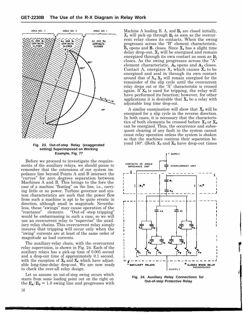
We have drawn the characteristics of two suchelements on our working example, as shown in Fig.23. In order to determine the practical operatingrequirements, we have used exaggerated settingsin this illustration. We will design each of theseelements with two contacts which we will desig-nate as No. 1 and No. 2. The No. 1 contact will beclosed whenever the apparent impedance falls tothe left of the element characteristic, while theNo. 2 contact will be closed whenever the apparentimpedance falls to the right of the element charac-teristic. For discussion purposes, we will call theleft element “A”, and the right element “B”, andshade those areas where each No. 1 contact isclosed. This has been done on Fig. 23 to show threedefinite areas :

Area No. l-contacts AS and B2 closed,Area No. 2nontacts A2 and B1 closed,Area No. 3-contacts A, and B, closed.

15


AREA NO. 3 AREA NO. 2 AREA NO. I

m:,,c--h---?,v

A2 AN0 BeCONTACTS

Fig. 23. Out-of-step Relay (exaggeratedsetting) Superimposed on Working

Example, Fig. 77

Before we proceed to investigate the require-ments of the auxiliary relays, we should pause toremember that the extensions of our system im-pedance line beyond Points A and B intersect the“curves” for zero degrees separation betweenMachines A and B. This brings to the fore thecase of a machine “floating” on the line, i.e., carry-ing little or no power. Turbine governor and sys-tem characteristics are such that the power flowfrom such a machine is apt to be quite erratic indirection, although small in magnitude. Neverthe-less, these “swings” may cause operation of the“reactance” elements. “Out-of -step tripping”would be embarrassing in such a case, so we willuse an overcurrent relay to “supervise” the auxil-iary relay chains. This overcurrent relay simplyinsures that tripping will occur only when the“swing” currents are at least of the same order ofmagnitude as load currents.

The auxiliary-relay chain, with the overcurrentrelay supervision, is shown in Fig. 24. Each of theauxiliary relays has a pick-up time of 0.005 secondand a drop-out time of approximately 0.1 second,with the exception of X3 and X6 which have adjust-able long-time-delay drop-out. We are now readyto check the over-all relay design.

Let us assume an out-of-step swing occurs whichstarts from some loading point out on the right onthe E,/E, = 1.0 swing line and progresses with

16

Machine A leading B. A, and Bz are closed initially,X, will pick-up through Bz, as soon as the overcur-rent relay closes its contacts. When the swingprogresses across the “B” element characteristic,B2 opens and B1 closes. Since X, has a slight timedelay drop-out, X2 will be energized and remainenergized through its own contact as soon as B1closes. As the swing progresses across the “A”element characteristic, A2 opens and A1 closes.Contact A, energizes X, which causes X3 to beenergized and seal in through its own contactaround that of X2. X3 will remain energized for theremainder of the slip cycle until the overcurrentrelay drops out or the “A” characteristic is crossedagain. If XS is used for tripping, the relay willhave performed its function; however, for otherapplications it is desirable that X3 be a relay withadjustable long time drop-out.

A similar examination will show that X6 will beenergized for a slip cycle in the reverse direction.In both cases, it is necessary that the characteris-tics of both elements be crossed before X3 or X0can be energized. Thus, the occurrence and subse-quent clearing of any fault in the system cannotcause relay operation unless the system is shakenso that the machines continue their separation be-yond 180°. (Both X8 and Xg have drop-out times

I+ SUPPLY

CONTACTS OF ANGLEIMPEDANCE UNIT OVERCURRENT UNIT

_----- - -_-_-_-r-LI

II

:I-_--

r---IIII

II

IIIIIII 4I

I

----1

i

: 02” I1 :------- q-IIAL-_--: AI* I

I

I

v--w-----_ _______

X4 X1

LbXl X5 x4

7 7,i, if- T

x3 xs X5

4

X3 X6 xs

---- J

l- ‘Aiili- i:Y; - - - - - - - - &&-Wi,, ,L;Y’

- S U P P L YDEENERGIZED

Fig. 24. Auxiliary Relay Connections forOut-of-step Protective Relay


MX’ 2 RELAY SETTING

A-S = SYSTEM IMPEDANCE

“A” & “B” ARE RELAY CHARACTERISTIC LINES

A8 * ANGULAR MOVEMENT BETWEEN A & BW H E N M O V I N G FROM X’ TO M TO X’

Fig. 25a. Geometric Relationship of Out-of-step Relay to System Characteristics

adjustable between 0.5 and 3.0 seconds. This as-sures that X3 will remain “picked-up” for all ex-cept the longest slip cycles and is useful where the“slip-directional” feature of the complete relay isused to change prime mover input.)

When Fig. 23 was introduced, the ohmic settingsof these “reactance” elements were said to beexaggerated. Let us investigate the requirementsfor these settings and plot the resultant settingson our working example.

The first requirement is that the relay operatefor the fastest slip cycle expected on the firstswing. The most critical operation then, is that ofclosing the contacts of Xz during the period whenthe swing is traversing the area between the “A”and “B” characteristics. Since X2 has a time-delayof 0.005 second in closing its contacts, the swingmust remain in this area at least 0.005 second. Theangle through which the system moves in travers-ing the area between the relay characteristics wewill call AS. Since the swing must take at least0.005 second to pass through this angle, the maxi-mum slip which will permit relay operation isgiven by the equation:

S,,, = &) x * , or;

S,,, = e slip cycles per second..

50

4 5

4 0

0 35

gYIJl 3 0

%

2 2 5

3zf 2 0

0d

IS

IO

5

OV , I I I0 0 .05 0.10 0.15 0

RELAY SETTING IN PER UNIT Of SYSTEM OHMS

Fig. 25b. Minimum Allowable Relay Set-ting for Operation of Out-of-step Relay

Versus Maximum Expected Slip

0

It remains to express AS in terms of the relay set-ting.

If we assume that the relay is located at a sta-tion which lies on the system impedance line andthat the relay characteristics parallel the systemimpedance line, we can show the relationshipsexisting between the relay setting, the system im-pedance, and the separation angle by the diagramshown in Fig. 25a. The separation angle, a, is theangle of separation between Machines A and B asdetermined by the intersection of the relay char-acteristic with the “equal-excitation-swing-line.”In Fig. 25a, AB is the system impedance, MX’ isthe relay setting (equal offset for each character-istic) and M is the mid-point of AB. In travelingfrom “B” to “A”, we must move from a systemangle of @J to 180° (Point M) to an equal angle onthe other side of 180°. Our total angular travel,AS, is thus equal to 2 x (180 - a), or:

AS=dx(go- $).

From the geometry of Fig. 25a, we see that the :

tan (90 - $ ) = z = MX’x2 or:AB


Substituting these values in the previous equa-tions, we can write :

s,,, = & tan-1 ( 2 x relay setting )

system ohms

From this last equation, we can plot a curve show-ing the relationship between the relay setting,expressed in per unit of system ohms, and themaximum expected slip which can give successfulrelay operation. This is shown in Fig. 25b.

Reference to Fig. 15 will show that the relaycharacteristics cover the least spread of separationangles at their intersection with the “equal-excita-tion-swing line.” This means that, all other thingsbeing equal, at constant slip speed the apparentimpedance will cross the relay characteristicsfaster for the condition of EA/EB = 1.0 than forany other excitation ratio.

The curve of Fig. 25b may be used with onlyslight theoretical error for those cases whereinthe relay “station” does not lie on the system im-pedance line, even for values of “per unit” relaysettings beyond 0.20. This is true because of therelative linearity of the tangent function for smallangles (less than 20 degrees).

The question naturally arises: “What would bethe maximum slip to be expected on the first swingcycle?” Any answer to this question would involvevarious system parameters and should be based ona transient stability study of the system underconsideration. Since we do not have such a studyavailable for the system used in our examples, wewill assume an answer based on experiences withother systems and on a rough approximation.

Investigation of several transient stability stud-ies made on the Network Analyzer in Schenectadyshows an average rotor velocity of 1.5 slip cyclesper second. This is in the region of 180° separationbetween that machine with greatest velocity andthe rest of the system. This gives us one benchmark.

Another bench mark may be found by a roughapproximation. One of the most severe cases intransient stability studies will be found in the con-dition of a direct three-phase fault on the termi-nals of a machine which had been fully loaded upto the instant of the fault. In this case, all of theprime mover torque is available for rotor accelera-tion except a small portion appearing as 12R lossin the armature windings. (This statement is truewithin the usual limits of a transient stabilitystudy. See reference 10 at rear of book.) As anexample in this case, we will investigate a 60 mega-watt preferred standard machine, fully loaded atthe 119 percent rating of the turbine, rated powerfactor and rated terminal voltage. Average perunit constants for this machine are:

18

X’d = 0.13 ra = 0.00111 H = 3.8(See reference 10 for definition of terms.)Machine loading is 0.935 + j0.58V’ = 1.0 + (0.935 - j0.58) (j0.13) = 1.083

1.083I’ = o 13 = 8.33.

(I’)2R, = 0.077

Turbine output = 0.935

Acceleration torque = 0.935 - 0.077 = 0.858

Acceleration constant = ‘““,: 6o = 2840”/Sec”.

Acceleration = 0 . 8 5 8 x 2840 = 2440”/Sec2

Under this constant acceleration, the time re-quired for the machine to advance 180” would be0.384 second and the velocity at that time would be938” per second or 2.6 slip cycles per second.These conditions are not directly applicable to ourproblem ; however, they do serve to furnish abench mark in selecting our relay setting.

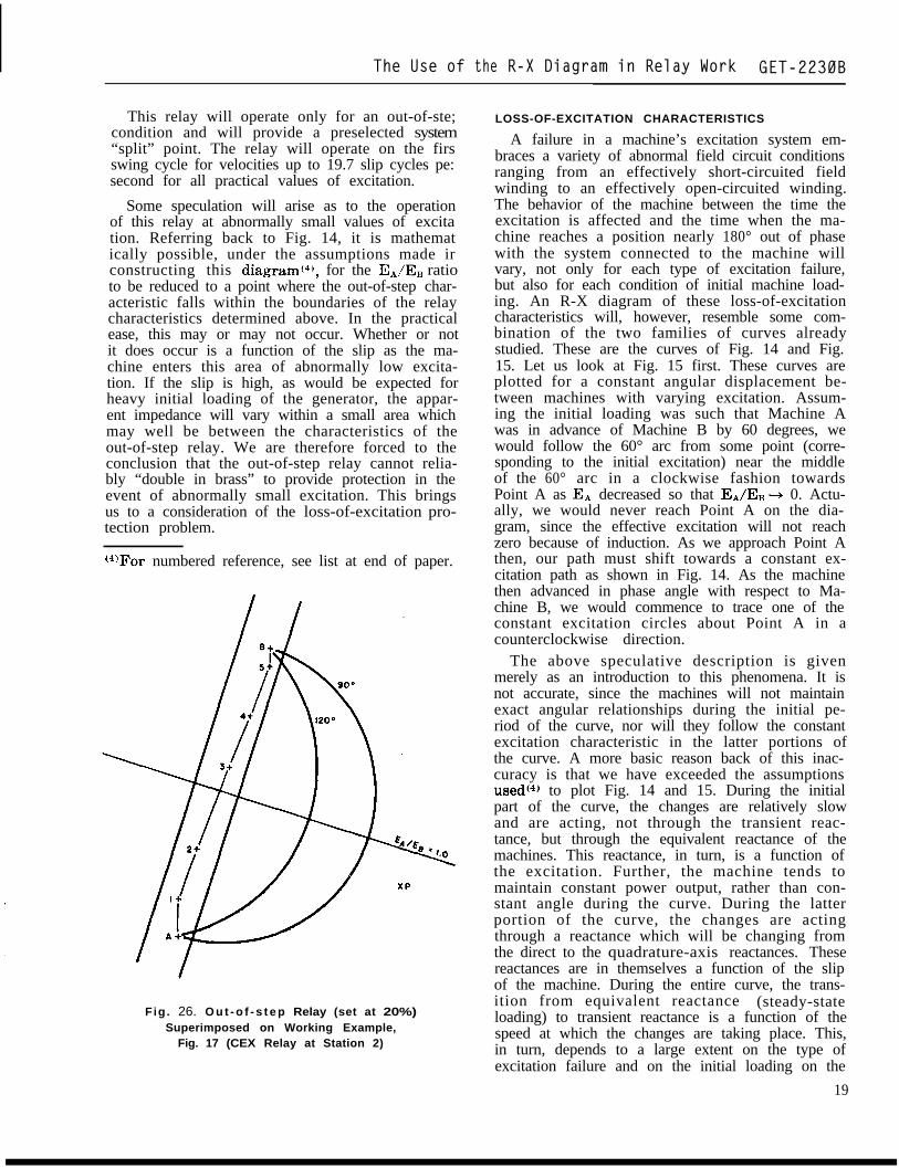
The second requirement for the relay setting isthat the relay characteristics should “blanket” thesystem plot on the R-X diagram. That is, a faultany place in the system should fall between therelay characteristics. As an illustration, let usrefer back to Fig. 23 and consider the applicationof this relay at Station 2. Since the relay charac-teristic will be offset an equal amount to each sideof Station 2 and will be parallel to the system im-pedance line (which lies to the right of Station 2),the right-hand characteristic shown on Fig. 23will be nearer the system R-X plot. An examina-tion of Fig. 23 leads us to select a setting of 1.25ohms. A plot of the resultant characteristic isshown in Fig. 26. It will be noted that the relaycharacteristics on Fig. 26 have a definite marginto clear all system faults and yet provide extraoperating margin by being well away from anystable operating area of the system.

If we investigate these settings in terms of theirintersection with the “equal-excitation-swingline,” as discussed previously, we find that “B”crosses at 168.5° and “A” crosses at 204°. Theangle enclosed is therefore 35.5°. The fastestswing which will cross these characteristics in0.005 second is one moving at 19.7 slip cycles persecond. Thus, this setting provides more than ade-quate margin for the fastest swings anticipated.(It is interesting to note that the chart of Fig. 25bgives an answer in close agreement with that cal-culated above. Our relay setting of 1.25 ohms,expressed in per unit of the system ohms (15.92)would be 0.0785. S,,, from Fig. 25b for this slip isbetween 19.5 and 20.0 slip cycles per second.)


This relay will operate only for an out-of-ste;condition and will provide a preselected system“split” point. The relay will operate on the firsswing cycle for velocities up to 19.7 slip cycles pe:second for all practical values of excitation.

Some speculation will arise as to the operationof this relay at abnormally small values of excitation. Referring back to Fig. 14, it is mathemat

ically possible, under the assumptions made irconstructing this diagramc4), for the EA/EH ratioto be reduced to a point where the out-of-step char-acteristic falls within the boundaries of the relaycharacteristics determined above. In the practicalease, this may or may not occur. Whether or notit does occur is a function of the slip as the ma-chine enters this area of abnormally low excita-tion. If the slip is high, as would be expected forheavy initial loading of the generator, the appar-ent impedance will vary within a small area whichmay well be between the characteristics of theout-of-step relay. We are therefore forced to theconclusion that the out-of-step relay cannot relia-bly “double in brass” to provide protection in theevent of abnormally small excitation. This bringsus to a consideration of the loss-of-excitation pro-tection problem.

(*)For numbered reference, see list at end of paper.

Fig. 26. O u t - o f - s t e p Relay (set at 20%)Superimposed on Working Example,

Fig. 17 (CEX Relay at Station 2)

LOSS-OF-EXCITATION CHARACTERISTICS

A failure in a machine’s excitation system em-braces a variety of abnormal field circuit conditionsranging from an effectively short-circuited fieldwinding to an effectively open-circuited winding.The behavior of the machine between the time theexcitation is affected and the time when the ma-chine reaches a position nearly 180° out of phasewith the system connected to the machine willvary, not only for each type of excitation failure,but also for each condition of initial machine load-ing. An R-X diagram of these loss-of-excitationcharacteristics will, however, resemble some com-bination of the two families of curves alreadystudied. These are the curves of Fig. 14 and Fig.15. Let us look at Fig. 15 first. These curves areplotted for a constant angular displacement be-tween machines with varying excitation. Assum-ing the initial loading was such that Machine Awas in advance of Machine B by 60 degrees, wewould follow the 60° arc from some point (corre-sponding to the initial excitation) near the middleof the 60° arc in a clockwise fashion towardsPoint A as EA decreased so that EA/EB + 0. Actu-ally, we would never reach Point A on the dia-gram, since the effective excitation will not reachzero because of induction. As we approach Point Athen, our path must shift towards a constant ex-citation path as shown in Fig. 14. As the machinethen advanced in phase angle with respect to Ma-chine B, we would commence to trace one of theconstant excitation circles about Point A in acounterclockwise direction.

The above speculative description is givenmerely as an introduction to this phenomena. It isnot accurate, since the machines will not maintainexact angular relationships during the initial pe-riod of the curve, nor will they follow the constantexcitation characteristic in the latter portions ofthe curve. A more basic reason back of this inac-curacy is that we have exceeded the assumptionsusedc4) to plot Fig. 14 and 15. During the initialpart of the curve, the changes are relatively slowand are acting, not through the transient reac-tance, but through the equivalent reactance of themachines. This reactance, in turn, is a function ofthe excitation. Further, the machine tends tomaintain constant power output, rather than con-stant angle during the curve. During the latterportion of the curve, the changes are actingthrough a reactance which will be changing fromthe direct to the quadrature-axis reactances. Thesereactances are in themselves a function of the slipof the machine. During the entire curve, the trans-ition from equivalent reactance (steady-stateloading) to transient reactance is a function of thespeed at which the changes are taking place. This,in turn, depends to a large extent on the type ofexcitation failure and on the initial loading on the

19


machine. When we try to include all of thesefactors in our problem, we find that the only prac-tical method for obtaining an analytical solution isby use of the differential analyzer.

From the differential analyzer, we have obtainedfour typical curves and sufficient additional data toenable us to proceed with our relay design. Thesecurves are shown in Fig. 27. This shows these fourcharacteristics plotted on an R-X diagram on aper-unit machine impedance base (e.g., the curvefor rated machine armature current at rated ter-minal voltage would be a circle centered on theorigin with a radius of 1.0/1.0 = 1.0 per unit im-pedance. For a more detailed discussion of thisbase, refer to Appendix A). (All of the subsequentR-X diagrams will be drawn to this base.) Eachcurve is marked at various points with referencenumbers showing the time in seconds for the char-acteristic to reach that point from the initial load-ing point with the excitation system failure oc-curring at t = 0. Each curve has been terminatedjust before the machine first reaches the 180°position with respect to the machine back of theequivalent system impedance. This has been doneonly for the sake of clarity, since the curves do notend at these points, but the changes in impedancefrom then on become so erratic that the curvecontinuation becomes useless for our purpose.

With the help of a little imagination, it is notdifficult to see that these curves are in generalagreement with the speculative curve discussedpreviously. What is more important, in our prob-lem of relay design, is that we have established a

definite locus of the “end points” of these curves.This locus is shown by the heavy curve on Fig. 27,which represents the average of the direct- andquadrature-axis impedances about which the endof the loss-of-excitation characteristic varies. Thisaverage impedance is low at high slip, approachingthe average of the direct-axis and quadrature-axissubtransient impedance of the generator. At verylow values of slip, the characteristic approachesthe average of the direct- and quadrature-axissynchronous impedances. These extremes are notactually reached, however.

We have established a curve which the loss-of-excitation characteristic must cross just beforethe affected machine passes 180° phase relation-ship with the system. Before we utilize this curvein designing our loss-of-excitation relay, we shouldinvestigate other abnormal, or normal, systemoperating characteristics which may approach thislocus, and for which it may not be desirable forthe loss-of-excitation relay to operate.

1. The first condition that comes to mind is thecase of a fault out in the system for which opera-tion of this relay would be undesirable. The sys-tem fault which approaches our loss-of-excitationlocus most closely is a generator bus fault. If wevisualize our loss-of-excitation relay as a single-phase relay (operated by line-to-line voltage andthe vector difference of line currents), the appar-ent impedance viewed by the relay for all types ofbus or system faults, lies in the region above theline MN(e) shown in Fig. 28. The line MN is per-pendicular to the generator impedance AO. Arc

+x

I1.0 -

INITIAL POINT100 % LOAD

INITIAL POINTAT 29.4% LOA0

AT: X=290, R=1.79)

2 . 0

t CURVE

_? @0000

SHORT CIRCUITED FIELD. 100 % LOAD, SMALL SYSTEM

SHORT CIRCUITED FIELD, 100 % LOAD, LARGE SYSTEM

OPEN CIRCUITED FIELD, 100% LOAD, LARGE SYSTEM

SHORT CIRCUITED FIELD, 29.4 % LOAD, LARGE SYSTEM

LOCUS OF AVERAGE IMPEDANCES JUST BEFOREI80° SEPARATION.

/GENERATOR

IMPEDANCE LINE

\

REGION IN WHICH IMPEDANCEVECTOR FALLS FOR BUS ORSYSTEM FAULT

\c +RN

20Fig. 27. Typical Loss-of-excitation Curves

and Average “Locus” Fig. 28. Faults External to Generator


resistance may cause the apparent impedance todrop below the line MN(@, but this deviation issmall and unimportant when we consider the nextcondition.

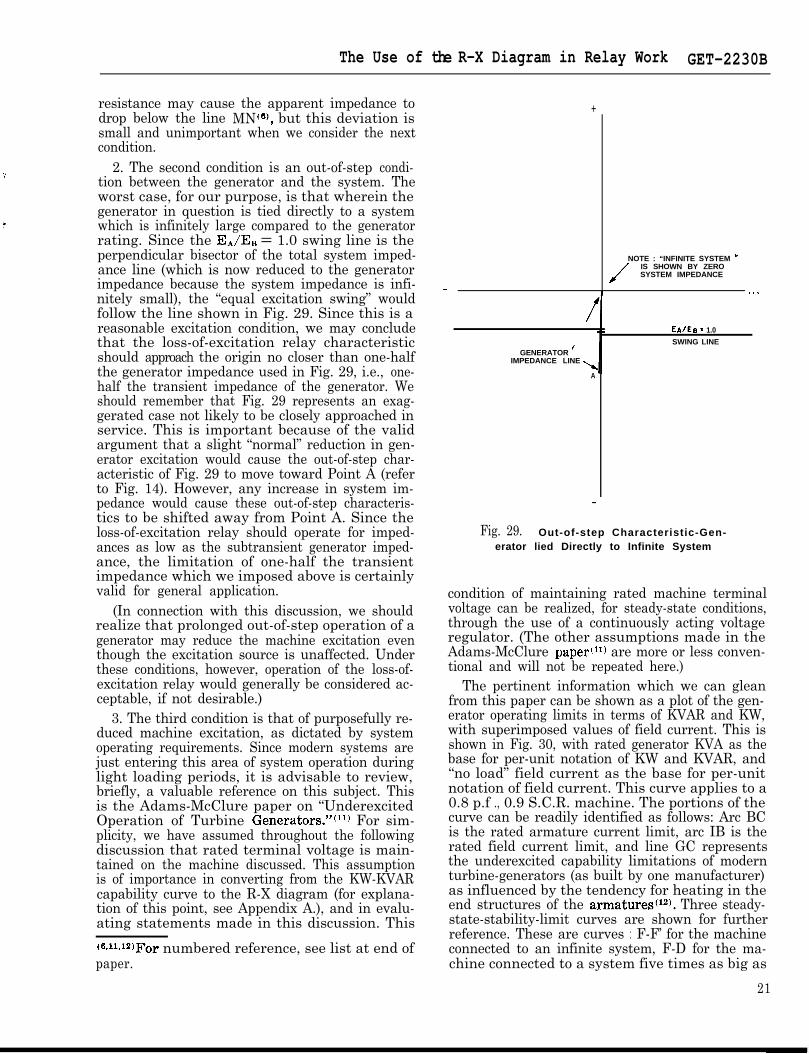
2. The second condition is an out-of-step condi-tion between the generator and the system. Theworst case, for our purpose, is that wherein thegenerator in question is tied directly to a systemwhich is infinitely large compared to the generatorrating. Since the E_JE, = 1.0 swing line is theperpendicular bisector of the total system imped-ance line (which is now reduced to the generatorimpedance because the system impedance is infi-nitely small), the “equal excitation swing” wouldfollow the line shown in Fig. 29. Since this is areasonable excitation condition, we may concludethat the loss-of-excitation relay characteristicshould approach the origin no closer than one-halfthe generator impedance used in Fig. 29, i.e., one-half the transient impedance of the generator. Weshould remember that Fig. 29 represents an exag-gerated case not likely to be closely approached inservice. This is important because of the validargument that a slight “normal” reduction in gen-erator excitation would cause the out-of-step char-acteristic of Fig. 29 to move toward Point A (referto Fig. 14). However, any increase in system im-pedance would cause these out-of-step characteris-tics to be shifted away from Point A. Since theloss-of-excitation relay should operate for imped-ances as low as the subtransient generator imped-ance, the limitation of one-half the transientimpedance which we imposed above is certainlyvalid for general application.

(In connection with this discussion, we shouldrealize that prolonged out-of-step operation of agenerator may reduce the machine excitation eventhough the excitation source is unaffected. Underthese conditions, however, operation of the loss-of-excitation relay would generally be considered ac-ceptable, if not desirable.)

3. The third condition is that of purposefully re-duced machine excitation, as dictated by systemoperating requirements. Since modern systems arejust entering this area of system operation duringlight loading periods, it is advisable to review,briefly, a valuable reference on this subject. Thisis the Adams-McClure paper on “UnderexcitedOperation of Turbine Generators.“(l’) For sim-plicity, we have assumed throughout the followingdiscussion that rated terminal voltage is main-tained on the machine discussed. This assumptionis of importance in converting from the KW-KVARcapability curve to the R-X diagram (for explana-tion of this point, see Appendix A.), and in evalu-ating statements made in this discussion. This

@J1J2)For numbered reference, see list at end ofpaper.

+

/

GENERATOR ’IMPEDANCE LINE

\A

NOTE : “INFINITE SYSTEM ”

J

IS SHOWN BY ZEROSYSTEM IMPEDANCE

. . .

EA/EB = 1.0

SWING LINE

Fig. 29. Out-of-step Characteristic-Gen-erator lied Directly to Infinite System

condition of maintaining rated machine terminalvoltage can be realized, for steady-state conditions,through the use of a continuously acting voltageregulator. (The other assumptions made in theAdams-McClure paper are more or less conven-tional and will not be repeated here.)

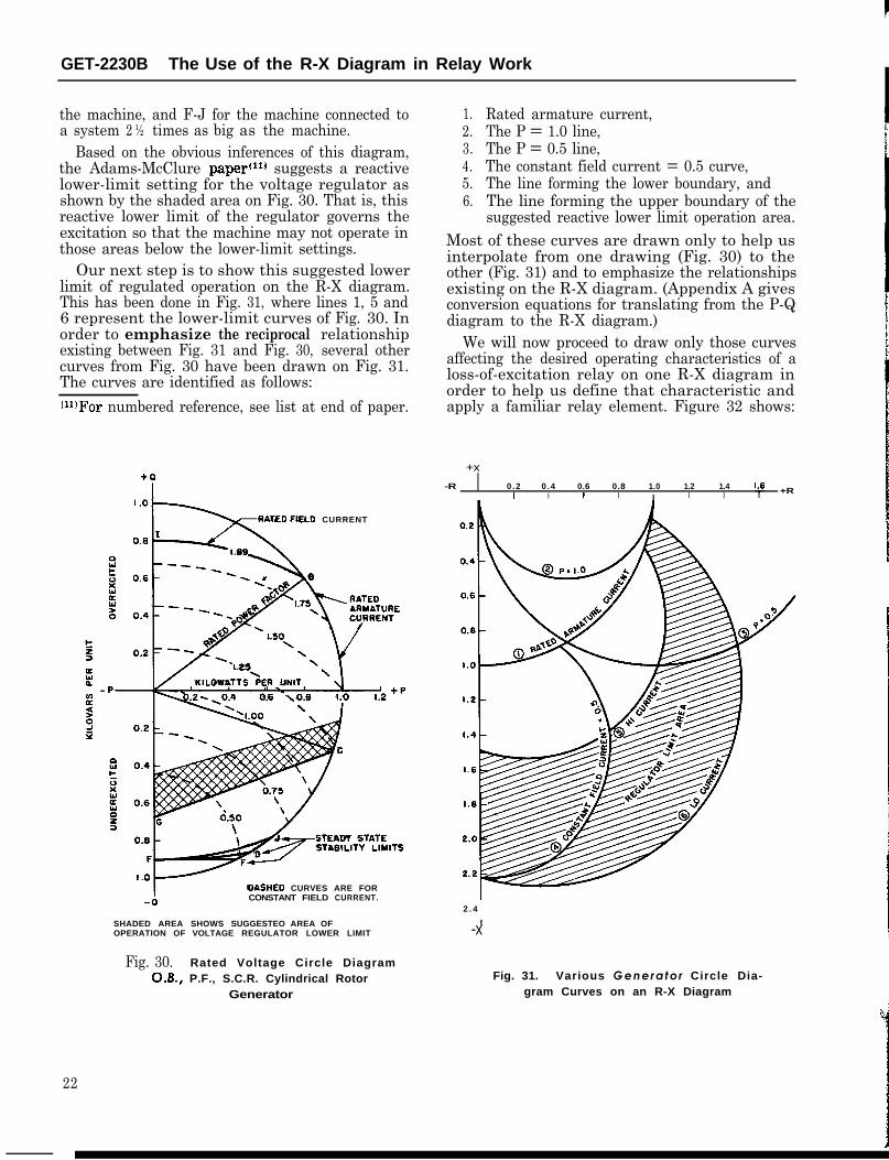
The pertinent information which we can gleanfrom this paper can be shown as a plot of the gen-erator operating limits in terms of KVAR and KW,with superimposed values of field current. This isshown in Fig. 30, with rated generator KVA as thebase for per-unit notation of KW and KVAR, and“no load” field current as the base for per-unitnotation of field current. This curve applies to a0.8 p.f ., 0.9 S.C.R. machine. The portions of thecurve can be readily identified as follows: Arc BCis the rated armature current limit, arc IB is therated field current limit, and line GC representsthe underexcited capability limitations of modernturbine-generators (as built by one manufacturer)as influenced by the tendency for heating in theend structures of the armatures(12). Three steady-state-stability-limit curves are shown for furtherreference. These are curves : F-F’ for the machineconnected to an infinite system, F-D for the ma-chine connected to a system five times as big as

21


the machine, and F-J for the machine connected toa system 2 ½ times as big as the machine.

Based on the obvious inferences of this diagram,the Adams-McClure paper<‘“) suggests a reactivelower-limit setting for the voltage regulator asshown by the shaded area on Fig. 30. That is, thisreactive lower limit of the regulator governs theexcitation so that the machine may not operate inthose areas below the lower-limit settings.

Our next step is to show this suggested lowerlimit of regulated operation on the R-X diagram.This has been done in Fig. 31, where lines 1, 5 and6 represent the lower-limit curves of Fig. 30. Inorder to emphasize the reciprocal relationshipexisting between Fig. 31 and Fig. 30, several othercurves from Fig. 30 have been drawn on Fig. 31.The curves are identified as follows:

(“)For numbered reference, see list at end of paper.

ATED F-0 CURRENT

~DASHED CURVES ARE FORCONSTANT FIELD CURRENT.

SHADED AREA SHOWS SUGGESTEO AREA OFOPERATION OF VOLTAGE REGULATOR LOWER LIMIT

1.2.3.4.5.6.

Rated armature current,The P = 1.0 line,The P = 0.5 line,The constant field current = 0.5 curve,The line forming the lower boundary, andThe line forming the upper boundary of thesuggested reactive lower limit operation area.

Most of these curves are drawn only to help usinterpolate from one drawing (Fig. 30) to theother (Fig. 31) and to emphasize the relationshipsexisting on the R-X diagram. (Appendix A givesconversion equations for translating from the P-Qdiagram to the R-X diagram.)

We will now proceed to draw only those curvesaffecting the desired operating characteristics of aloss-of-excitation relay on one R-X diagram inorder to help us define that characteristic andapply a familiar relay element. Figure 32 shows:

+x

-R 0.2 0 .4 0.6 0.8 1.0 1.2 1.4I I I I I I I ‘i” +R

2 . 4

t-x

Fig. 30. Rated Voltage Circle DiagramO.B., P.F., S.C.R. Cylindrical Rotor

Generator

Fig. 31. Various Generator Circle Dia-gram Curves on an R-X Diagram

22


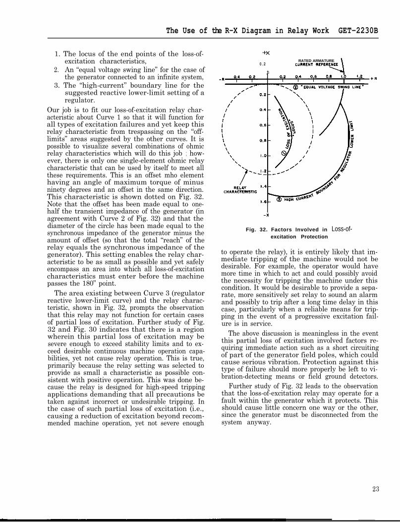
1. The locus of the end points of the loss-of-excitation characteristics,

2. An “equal voltage swing line” for the case ofthe generator connected to an infinite system,

3. The “high-current” boundary line for thesuggested reactive lower-limit setting of aregulator.

Our job is to fit our loss-of-excitation relay char-acteristic about Curve 1 so that it will function forall types of excitation failures and yet keep thisrelay characteristic from trespassing on the “off-limits” areas suggested by the other curves. It ispossible to visualize several combinations of ohmicrelay characteristics which will do this job ; how-ever, there is only one single-element ohmic relaycharacteristic that can be used by itself to meet allthese requirements. This is an offset mho elementhaving an angle of maximum torque of minusninety degrees and an offset in the same direction.This characteristic is shown dotted on Fig. 32.Note that the offset has been made equal to one-half the transient impedance of the generator (inagreement with Curve 2 of Fig. 32) and that thediameter of the circle has been made equal to thesynchronous impedance of the generator minus theamount of offset (so that the total “reach” of therelay equals the synchronous impedance of thegenerator). This setting enables the relay char-acteristic to be as small as possible and yet safelyencompass an area into which all loss-of-excitationcharacteristics must enter before the machinepasses the 180” point.

The area existing between Curve 3 (regulatorreactive lower-limit curve) and the relay charac-teristic, shown in Fig. 32, prompts the observationthat this relay may not function for certain casesof partial loss of excitation. Further study of Fig.32 and Fig. 30 indicates that there is a regionwherein this partial loss of excitation may besevere enough to exceed stability limits and to ex-ceed desirable continuous machine operation capa-bilities, yet not cause relay operation. This is true,primarily because the relay setting was selected toprovide as small a characteristic as possible con-sistent with positive operation. This was done be-cause the relay is designed for high-speed trippingapplications demanding that all precautions betaken against incorrect or undesirable tripping. Inthe case of such partial loss of excitation (i.e.,causing a reduction of excitation beyond recom-mended machine operation, yet not severe enough

+x

0.2

t

RATED ARMATURE

CHARACTERISTIC

+R

-x

Fig. 32. Factors Involved inexcitation Protection

Loss-of-

to operate the relay), it is entirely likely that im-mediate tripping of the machine would not bedesirable. For example, the operator would havemore time in which to act and could possibly avoidthe necessity for tripping the machine under thiscondition. It would be desirable to provide a sepa-rate, more sensitively set relay to sound an alarmand possibly to trip after a long time delay in thiscase, particularly when a reliable means for trip-ping in the event of a progressive excitation fail-ure is in service.

The above discussion is meaningless in the eventthis partial loss of excitation involved factors re-quiring immediate action such as a short circuitingof part of the generator field poles, which couldcause serious vibration. Protection against thistype of failure should more properly be left to vi-bration-detecting means or field ground detectors.

Further study of Fig. 32 leads to the observationthat the loss-of-excitation relay may operate for afault within the generator which it protects. Thisshould cause little concern one way or the other,since the generator must be disconnected from thesystem anyway.

23


APPENDIX A

PER-UNIT NOTATIONThe calculation of machine or system perfor-

mance may be simplified by the use of per-unitrepresentation of all quantities such as voltage,current, impedance, power, or KVA. Thus, a se-lected base value is considered as unit, or 1.0, andall quantities expressed as a ratio in decimal formwith respect to the base value of the quantity. Forconvenience, it has been the practice to select acommon base KVA and use with the rated line-to-line voltage as the independent base quantities.The relationship of other base quantities is deter-mined by these equations :

Base KVABase Amps = ,/3 Base KV

Base Ohms = L-G KV x lo3Base AmpsBase KV x lo3

= ~‘3 Base Amps

= Base KV2 x 10”Base KVA

Base KW = Base KVAR = Base KVAand so forth.

For example, a 60,000-KW preferred standardturbine-generator operating at the 110 percentturbine rating, at rated 0.85 p.f., will have an out-put of 66,000 KW and 40,900 KVAR, or 77,600KVA. For a machine operating at its rated voltage,assuming that voltage to be 14 KV, the currentflowing would be 2720 - j1690 or 3200 amperes.The series load impedance causing this flow wouldbe 2.15 ohms resistance and 1.33 ohms reactance.

To express these quantities in per unit based onthe machine’s ½ psi H, rating and rated voltage :Base KVA = 70,600 KVA, Base K V = 14 KV, BaseAmperes = 2910 amps, Base ohms = 2.78 ohms.Converting the flow figures determined above toper unit: P = 0.935, Q = 0.580, KVA = 1.1, I =0.935 - j0.580 = 1.1 and the series load impedanceis 0.77 per-unit resistance and 0.48 per-unit reac-tance.

Where per-unit quantities are used throughout,the conversion becomes more straightforward.

Let us represent the load flow by the followingdiagram :

Q(Q) + ‘v

-

The following relationships hold :

I= 7 and I2 = if&_@

R = $ = p2p+v2Q2

In the above example then:

R = 0.935 x (1.d) 2(1.1)s

= 0 * 772

2x = 0.580 42 x 1.0 ) = 0.480

Conversion from per-unit diagrams, i.e., P-Q toR-X or vice versa, can be easily accomplished bythe following equations :

PV”R = P2 + Q”

x = p2Q;$,

p= RV”R” + X2

Q= xv2R2 + X2

These equations may also be used for actualvalues, in which case it is imperative that consis-tent units be used.

Thus :

R = line-to-neutral resistance in ohmsX = line-to-neutral reactance in ohmsV = line-to-line voltage in voltsP = 3-phase power, supplied by generator to sys-

tem, in wattsQ = 3-phase vars, supplied by “overexcited” gen-

erator to system for positive values, involt-amperes.

(The above are all positive phase sequence values.)

24


CONCLUSION tionships in the complex field of modern relaying.We have seen that the R-X diagram is an essen- This has been a hurried and limited trip through

tial tool in the comparison, evaluation, and appli- the features of the R-X diagram as applied to re-cation of distance relays. (It is also essential in lays. Many simplifying assumptions have beennumerous other fields not covered in this discus- made and many interesting relay applications havesion.) The diagram is easy to construct and lends been avoided. For those of you who are interesteditself to a simultaneous plot of system conditions in further exploration of the possibilities of theand relay characteristics with a simplicity of geo- R-X diagram, we recommend, most wholeheart-metric constructions. By its simplicity, it offers a edly, Miss Clarke’s excellent paper on this subject.readily understandable picture of complex rela- Full reference information follows:

1.

2.

3.

4.

5.

6.

GENERAL SPECIFIC RELAY APPLICATIONSRelay Operation During System Oscillations,C. R. Mason. AIEE Transactions, Vol. 56,1937, pp. 823-832.

7.

Discussion by J. H. Neher, pp. 1513-1514.Closing Discussion by C. R. Mason, Vol. 57,1938, pp. 111-114.

A New Loss-of-Excitation Relay for Synchro-nous Generators, C. R. Mason. AIEE Techni-cal Paper 49-260, presented at the AIEE FallGeneral Meeting, Cincinnati, Ohio, October,1949.

8.A Comprehensive Method of Determining thePerformance of Distance Relays, J. H. Neher.AIEE Transactions, Vol. 56, 1937, pp. 833-844.

Performance Requirements for Relays on Un-usually Long Transmission Lines, F. C. Poage,C. A. Streifus, D. M. MacGregor, and E. E.George. AIEE Transactions, Vol. 62, 1943,p. 275.

9.

10.

11.

12.

A One Slip Cycle Out-of-Step Relay Equip-ment, W. C. Morris, AIEE Technical Paper49-261, presented at the AIEE Fall GeneralMeeting, Cincinnati, Ohio, October, 1949.

Combined Phase and Ground Distance Relay-ing, Warren C. New. AIEE Technical Paper50-7, presented at the AIEE Winter GeneralMeeting, New York, N.Y., January, 1950.

Impedances Seen by Relays During PowerSwings With and Without Faults, EdithClarke. AIEE Transactions, Vol. 64, 1945,pp. 372-384.

G-E Network Analyzers, An A. C. NetworkAnalyzer Manual compiled by the AnalyticalDivision ; Applications, Service, and Construc-tion Engineering Divisions ; General ElectricCompany, General Electric Publication No.GET-1285A.

Discussion of reference 4, A. J. McConnell.AIEE Transaction, June Supplement, 1945,p. 472.

Graphical Method for Estimating the Perfor-mance of Distance Relays During Faults andPower Swings, A. R. van C. Warrington.AIEE Technical Paper 49-154, presented atthe AIEE Summer Convention, Swampscott,Mass., June, 1949.

Underexcited Operation of Turbine Genera-tors, C. G. Adams, J. B. McClure, AIEE Tech-nical Paper 48-81, presented at the AIEEWinter General Meeting, Pittsburgh, Pa.,January, 1948.

Operation of Turbine Generators with LowField Currents, J. H. Carter, AIEE ConferencePaper, presented at the AIEE Winter GeneralMeeting, New York, N.Y., January, 1950.

25

��*(�3RZHU�0DQDJHPHQW

215 Anderson AvenueMarkham, OntarioCanada L6E 1B3Tel: (905) 294-6222Fax: (905) 201-2098www.GEindustrial.com/pm

use of the r-x diagram in relay work

Documents