This publication is intended to serve as both a guidebook and introductory tutorial for the use of mathematical modelling (using mostly Monte Carlo methods) in electron beam processing. The emphasis of this guide is on industrial irradiation methodologies, with extensive reference to existing literature and applicable standards. Its target audience is readers who have a basic understanding of electron beam technology and want to evaluate and apply mathematical modelling for the design and operation of irradiators, and those who wish to have a better understanding of irradiation methodology and process development for new products.

INTERNATIONAL ATOMIC ENERGY AGENCYVIENNA

ISBN 978–92–0–112010–6ISSN 2220–7341

IAEA RAD

IATION

TECH

NO

LOGY SER

IES No. 1

IAEA RADIATION TECHNOLOGY SERIES No. 1

Use of Mathematical Modelling in Electron Beam Processing: A Guidebook

10-38771_P1474_cover.indd 1 2011-01-14 14:43:06

IAEA RADIATION TECHNOLOGY SERIES PUBLICATIONS

One of the main objectives of the IAEA Radioisotope Production and Radiation Technology programme is to enhance the expertise and capability of IAEA Member States in utilizing the methodologies for radiation processing, compositional analysis and industrial applications of radioisotope techniques in order to meet national needs as well as to assimilate new developments for improving industrial process efficiency and safety, development and characterization of value-added products, and treatment of pollutants/hazardous materials.

Publications in the IAEA Radiation Technology Series provide information in the areas of: radiation processing and characterization of materials using ionizing radiation, and industrial applications of radiotracers, sealed sources and non-destructive testing. The publications have a broad readership and are aimed at meeting the needs of scientists, engineers, researchers, teachers and students, laboratory professionals, and instructors. International experts assist the IAEA Secretariat in drafting and reviewing these publications. Some of the publications in this series may also be endorsed or co-sponsored by international organizations and professional societies active in the relevant fields.

There are two categories of publications: the IAEA Radiation Technology Series and the IAEA Radiation Technology Reports.

IAEA RADIATION TECHNOLOGY SERIES

Publications in this category present guidance information or methodologies and analyses of long term validity, for example protocols, guidelines, codes, standards, quality assurance manuals, best practices and high level technological and educational material.

IAEA RADIATION TECHNOLOGY REPORTS

In this category, publications complement information published in the IAEA Radiation Technology Series in the areas of: radiation processing of materials using ionizing radiation, and industrial applications of radiotracers, sealed sources and NDT. These publications include reports on current issues and activities such as technical meetings, the results of IAEA coordinated research projects, interim reports on IAEA projects, and educational material compiled for IAEA training courses dealing with radioisotope and radiopharmaceutical related subjects. In some cases, these reports may provide supporting material relating to publications issued in the IAEA Radiation Technology Series.

All of these publications can be downloaded cost free from the IAEA web site:

http://www.iaea.org/Publications/index.html

Further information is available from:

Marketing and Sales UnitInternational Atomic Energy AgencyVienna International CentrePO Box 1001400 Vienna, Austria

Readers are invited to provide feedback to the IAEA on these publications. Information may be provided through the IAEA web site, by mail at the address given above, or by email to:

Official.Mail@iaea.org

10-38771_P1474_cover.indd 2 2011-01-19 09:43:49

USE OFMATHEMATICAL MODELLING INELECTRON BEAM PROCESSING:

A GUIDEBOOK

The following States are Members of the International Atomic Energy Agency:

AFGHANISTANALBANIAALGERIAANGOLAARGENTINAARMENIAAUSTRALIAAUSTRIAAZERBAIJANBAHRAINBANGLADESHBELARUSBELGIUMBELIZEBENINBOLIVIABOSNIA AND HERZEGOVINABOTSWANABRAZILBULGARIABURKINA FASOBURUNDICAMBODIACAMEROONCANADACENTRAL AFRICAN

REPUBLICCHADCHILECHINACOLOMBIACONGOCOSTA RICACÔTE D’IVOIRECROATIACUBACYPRUSCZECH REPUBLICDEMOCRATIC REPUBLIC

OF THE CONGODENMARKDOMINICAN REPUBLICECUADOREGYPTEL SALVADOR

GHANAGREECEGUATEMALAHAITIHOLY SEEHONDURASHUNGARYICELANDINDIAINDONESIAIRAN, ISLAMIC REPUBLIC OF IRAQIRELANDISRAELITALYJAMAICAJAPANJORDANKAZAKHSTANKENYAKOREA, REPUBLIC OFKUWAITKYRGYZSTANLATVIALEBANONLESOTHOLIBERIALIBYAN ARAB JAMAHIRIYALIECHTENSTEINLITHUANIALUXEMBOURGMADAGASCARMALAWIMALAYSIAMALIMALTAMARSHALL ISLANDSMAURITANIAMAURITIUSMEXICOMONACOMONGOLIAMONTENEGROMOROCCOMOZAMBIQUE

NORWAYOMANPAKISTANPALAUPANAMAPARAGUAYPERUPHILIPPINESPOLANDPORTUGALQATARREPUBLIC OF MOLDOVAROMANIARUSSIAN FEDERATIONSAUDI ARABIASENEGALSERBIASEYCHELLESSIERRA LEONESINGAPORESLOVAKIASLOVENIASOUTH AFRICASPAINSRI LANKASUDANSWEDENSWITZERLANDSYRIAN ARAB REPUBLICTAJIKISTANTHAILANDTHE FORMER YUGOSLAV

REPUBLIC OF MACEDONIATUNISIATURKEYUGANDAUKRAINEUNITED ARAB EMIRATESUNITED KINGDOM OF

GREAT BRITAIN AND NORTHERN IRELAND

UNITED REPUBLIC OF TANZANIA

The Agency’s Statute was approved on 23 October 1956 by the Conference on the Statute of thIAEA held at United Nations Headquarters, New York; it entered into force on 29 July 1957. ThHeadquarters of the Agency are situated in Vienna. Its principal objective is “to accelerate and enlarge thcontribution of atomic energy to peace, health and prosperity throughout the world’’.

ERITREAESTONIAETHIOPIAFINLANDFRANCEGABONGEORGIAGERMANY

MYANMARNAMIBIANEPAL NETHERLANDSNEW ZEALANDNICARAGUANIGERNIGERIA

UNITED STATES OF AMERICAURUGUAYUZBEKISTANVENEZUELAVIETNAMYEMENZAMBIAZIMBABWE

e e e

IAEA RADIATION TECHNOLOGY SERIES No. 1

USE OFMATHEMATICAL MODELLING INELECTRON BEAM PROCESSING:

A GUIDEBOOK

INTERNATIONAL ATOMIC ENERGY AGENCYVIENNA, 2010

IAEA Library Cataloguing in Publication Data

Use of mathematical modelling in electron beam processing : a guidebook. — Vienna : International Atomic Energy Agency, 2010.

p. ; 24 cm. — (IAEA radiation technology series, ISSN 2220–7341 ; no. 1)STI/PUB/1474

COPYRIGHT NOTICE

All IAEA scientific and technical publications are protected by the terms of the Universal Copyright Convention as adopted in 1952 (Berne) and as revised in 1972 (Paris). The copyright has since been extended by the World Intellectual Property Organization (Geneva) to include electronic and virtual intellectual property. Permission to use whole or parts of texts contained in IAEA publications in printed or electronic form must be obtained and is usually subject to royalty agreements. Proposals for non-commercial reproductions and translations are welcomed and considered on a case-by-case basis. Enquiries should be addressed to the IAEA Publishing Section at:

Marketing and Sales Unit, Publishing SectionInternational Atomic Energy AgencyVienna International CentrePO Box 1001400 Vienna, Austriafax: +43 1 2600 29302tel.: +43 1 2600 22417email: sales.publications@iaea.org http://www.iaea.org/books

© IAEA, 2010

Printed by the IAEA in AustriaDecember 2010STI/PUB/1474

ISBN 978–92–0–112010–6Includes bibliographical references.

1. Electron beams — Industrial applications. — 2. Electron beams — Mathematical models. — 3. Monte Carlo method. I. International Atomic Energy Agency. II. Series.

IAEAL 11–00664

FOREWORD

The use of electron beam irradiation for industrial applications, like the sterilization of medical devices or cross-linking of polymers, has a long and successful track record and has proven itself to be a key technology. Emerging fields, including environmental applications of ionizing radiation, the sterilization of complex medical and pharmaceutical products or advanced material treatment, require the design and control of even more complex irradiators and irradiation processes.

Mathematical models can aid the design process, for example by calculating absorbed dose distributions in a product, long before any prototype is built. They support process qualification through impact assessment of process variable uncertainties, and can be an indispensable teaching tool for technologists in training in the use of radiation processing.

The IAEA, through various mechanisms, including its technical cooperation programme, coordinated research projects, technical meetings, guidelines and training materials, is promoting the use of radiation technologies to minimize the effects of harmful contaminants and develop value added products originating from low cost natural and human made raw materials.

The need to publish a guidebook on the use of mathematical modelling for design processes in the electron beam treatment of materials was identified through the increased interest of radiation processing laboratories in Member States and as a result of recommendations from several IAEA expert meetings. In response, the IAEA has prepared this report using the services of an expert in the field.

This publication should serve as both a guidebook and introductory tutorial for the use of mathematical modelling (using mostly Monte Carlo methods) in electron beam processing. The emphasis of this guide is on industrial irradiation methodologies with a strong reference to existing literature and applicable standards. Its target audience is readers who have a basic understanding of electron beam technology and want to evaluate and apply mathematical modelling for the design and operation of irradiators, and those who wish to have a better understanding of irradiation methodology and process development for new products.

The IAEA wishes to thank J. Mittendorfer (Austria) for sharing his expertise, and for his contribution to the preparation of this report. The IAEA

officers responsible for this publication were M. Haji-Saeid and M.H.O. Sampa of the Division of Physical and Chemical Sciences.

CONTENTS

1. INTRODUCTION . . . . . . . . . . . . . . . . . . . . . . . . . . . . . . . . . . . . . . . . 1

1.1. Background . . . . . . . . . . . . . . . . . . . . . . . . . . . . . . . . . . . . . . . . . 11.2. Objective . . . . . . . . . . . . . . . . . . . . . . . . . . . . . . . . . . . . . . . . . . . 11.3. Scope. . . . . . . . . . . . . . . . . . . . . . . . . . . . . . . . . . . . . . . . . . . . . . 2

2. OVERVIEW OF ELECTRON BEAM PROCESSING. . . . . . . . . . . . 2

2.1. Components of an electron beam system . . . . . . . . . . . . . . . . . . 32.1.1. The electron source . . . . . . . . . . . . . . . . . . . . . . . . . . . . . 32.1.2. Product handling . . . . . . . . . . . . . . . . . . . . . . . . . . . . . . . 32.1.3. Shielding . . . . . . . . . . . . . . . . . . . . . . . . . . . . . . . . . . . . . 42.1.4. Beam stop . . . . . . . . . . . . . . . . . . . . . . . . . . . . . . . . . . . . 42.1.5. Support units . . . . . . . . . . . . . . . . . . . . . . . . . . . . . . . . . . 5

2.2. Accelerator types and performance parameters . . . . . . . . . . . . . 52.2.1. Classification. . . . . . . . . . . . . . . . . . . . . . . . . . . . . . . . . . 62.2.2. Beam energy . . . . . . . . . . . . . . . . . . . . . . . . . . . . . . . . . . 62.2.3. Beam specification . . . . . . . . . . . . . . . . . . . . . . . . . . . . . 7

2.3. Product handling systems . . . . . . . . . . . . . . . . . . . . . . . . . . . . . . 102.4. Process variables. . . . . . . . . . . . . . . . . . . . . . . . . . . . . . . . . . . . . 11

2.4.1. Beam energy . . . . . . . . . . . . . . . . . . . . . . . . . . . . . . . . . . 122.4.2. Beam current . . . . . . . . . . . . . . . . . . . . . . . . . . . . . . . . . . 122.4.3. Product speed . . . . . . . . . . . . . . . . . . . . . . . . . . . . . . . . . 122.4.4. Scan width and scan distribution . . . . . . . . . . . . . . . . . . 122.4.5. Distance to product . . . . . . . . . . . . . . . . . . . . . . . . . . . . . 132.4.6. Beam geometry . . . . . . . . . . . . . . . . . . . . . . . . . . . . . . . . 132.4.7. Design specifications of an electron beam system . . . . . 132.4.8. System geometry and materials . . . . . . . . . . . . . . . . . . . 132.4.9. Process parameters . . . . . . . . . . . . . . . . . . . . . . . . . . . . . 14

3. MATHEMATICAL MODELS USED IN ELECTRONBEAM PROCESSING. . . . . . . . . . . . . . . . . . . . . . . . . . . . . . . . . . . . . 14

3.1. Introduction. . . . . . . . . . . . . . . . . . . . . . . . . . . . . . . . . . . . . . . . . 143.2. Mathematical models of irradiation processing . . . . . . . . . . . . . 15

3.2.1. Deterministic methods . . . . . . . . . . . . . . . . . . . . . . . . . . 163.2.2. Semi-empirical methods . . . . . . . . . . . . . . . . . . . . . . . . . 16

3.2.3. Empirical methods . . . . . . . . . . . . . . . . . . . . . . . . . . . . . 163.2.4. Monte Carlo methods . . . . . . . . . . . . . . . . . . . . . . . . . . . 16

3.3. Interaction of photons with matter . . . . . . . . . . . . . . . . . . . . . . . 173.3.1. Introduction. . . . . . . . . . . . . . . . . . . . . . . . . . . . . . . . . . . 173.3.2. Photo effect . . . . . . . . . . . . . . . . . . . . . . . . . . . . . . . . . . . 183.3.3. Compton scattering . . . . . . . . . . . . . . . . . . . . . . . . . . . . . 183.3.4. Pair production . . . . . . . . . . . . . . . . . . . . . . . . . . . . . . . . 183.3.5. Elastic scattering . . . . . . . . . . . . . . . . . . . . . . . . . . . . . . . 183.3.6. The concept of free path length. . . . . . . . . . . . . . . . . . . . 19

3.4. Interaction of electrons with matter . . . . . . . . . . . . . . . . . . . . . . 193.4.1. Introduction. . . . . . . . . . . . . . . . . . . . . . . . . . . . . . . . . . . 193.4.2. Elastic scattering . . . . . . . . . . . . . . . . . . . . . . . . . . . . . . . 193.4.3. Energy loss by ionization . . . . . . . . . . . . . . . . . . . . . . . . 193.4.4. Energy loss by bremsstrahlung . . . . . . . . . . . . . . . . . . . . 203.4.5. Annihilation . . . . . . . . . . . . . . . . . . . . . . . . . . . . . . . . . . 203.4.6. Monte Carlo simulation of electron interaction . . . . . . . 20

4. THE MONTE CARLO METHOD . . . . . . . . . . . . . . . . . . . . . . . . . . . 21

4.1. Introduction. . . . . . . . . . . . . . . . . . . . . . . . . . . . . . . . . . . . . . . . . 214.1.1. The Monte Carlo method — An introductory

example . . . . . . . . . . . . . . . . . . . . . . . . . . . . . . . . . . . . . . 214.2. Random numbers . . . . . . . . . . . . . . . . . . . . . . . . . . . . . . . . . . . . 24

4.2.1. Introduction. . . . . . . . . . . . . . . . . . . . . . . . . . . . . . . . . . . 244.2.2. Pseudo random number generators . . . . . . . . . . . . . . . . . 24

4.3. Sampling probability distribution functions . . . . . . . . . . . . . . . . 254.3.1. Inversion method. . . . . . . . . . . . . . . . . . . . . . . . . . . . . . . 264.3.2. Rejection method . . . . . . . . . . . . . . . . . . . . . . . . . . . . . . 284.3.3. Sampling from a histogram. . . . . . . . . . . . . . . . . . . . . . . 29

5. MONTE CARLO TRANSPORT CODES. . . . . . . . . . . . . . . . . . . . . . 32

5.1. Introduction. . . . . . . . . . . . . . . . . . . . . . . . . . . . . . . . . . . . . . . . . 325.2. Monte Carlo transport code applications . . . . . . . . . . . . . . . . . . 33

5.2.1. Medical applications . . . . . . . . . . . . . . . . . . . . . . . . . . . . 335.2.2. Radiation protection and shielding calculation. . . . . . . . 34

5.2.3. Space applications. . . . . . . . . . . . . . . . . . . . . . . . . . . . . . 355.2.4. High energy physics . . . . . . . . . . . . . . . . . . . . . . . . . . . . 355.2.5. Industrial applications . . . . . . . . . . . . . . . . . . . . . . . . . . . 35

5.3. Survey of codes. . . . . . . . . . . . . . . . . . . . . . . . . . . . . . . . . . . . . . 365.3.1. Code distribution. . . . . . . . . . . . . . . . . . . . . . . . . . . . . . . 365.3.2. EGSnrc and beam . . . . . . . . . . . . . . . . . . . . . . . . . . . . . . 365.3.3. PENELOPE. . . . . . . . . . . . . . . . . . . . . . . . . . . . . . . . . . . 375.3.4. Integrated Tiger System (ITS) . . . . . . . . . . . . . . . . . . . . 375.3.5. RT Office 2.0. . . . . . . . . . . . . . . . . . . . . . . . . . . . . . . . . . 385.3.6. MCNPX . . . . . . . . . . . . . . . . . . . . . . . . . . . . . . . . . . . . . 385.3.7. GEANT4 . . . . . . . . . . . . . . . . . . . . . . . . . . . . . . . . . . . . . 38

5.4. Basic Monte Carlo code modules . . . . . . . . . . . . . . . . . . . . . . . . 395.5. Geometry input . . . . . . . . . . . . . . . . . . . . . . . . . . . . . . . . . . . . . . 40

5.5.1. Data driven input using text files . . . . . . . . . . . . . . . . . . 415.5.2. Data driven input by GUI . . . . . . . . . . . . . . . . . . . . . . . . 415.5.3. Programmatic input. . . . . . . . . . . . . . . . . . . . . . . . . . . . . 435.5.4. CAD interface . . . . . . . . . . . . . . . . . . . . . . . . . . . . . . . . . 46

5.6. Material definition . . . . . . . . . . . . . . . . . . . . . . . . . . . . . . . . . . . 475.7. The physics model . . . . . . . . . . . . . . . . . . . . . . . . . . . . . . . . . . . 495.8. Tracking . . . . . . . . . . . . . . . . . . . . . . . . . . . . . . . . . . . . . . . . . . . 495.9. Cut-offs . . . . . . . . . . . . . . . . . . . . . . . . . . . . . . . . . . . . . . . . . . . . 525.10. Detectors and hits . . . . . . . . . . . . . . . . . . . . . . . . . . . . . . . . . . . . 535.11. From energy deposition to dose . . . . . . . . . . . . . . . . . . . . . . . . . 545.12. Uncertainty in Monte Carlo calculations . . . . . . . . . . . . . . . . . . 575.13. Variance reduction techniques . . . . . . . . . . . . . . . . . . . . . . . . . . 615.14. Verification and validation . . . . . . . . . . . . . . . . . . . . . . . . . . . . . 62

6. CALCULATIONS USING ONE DIMENSIONALMATHEMATICAL MODELLING. . . . . . . . . . . . . . . . . . . . . . . . . . . 64

6.1. Introduction. . . . . . . . . . . . . . . . . . . . . . . . . . . . . . . . . . . . . . . . . 646.2. Stopping power and depth–dose curves . . . . . . . . . . . . . . . . . . . 646.3. Example 1: One dimensional aluminium slab . . . . . . . . . . . . . . 66

6.3.1. The TIGER cross-section file . . . . . . . . . . . . . . . . . . . . . 686.3.2. The TIGER geometry and simulation control file . . . . . 706.3.3. The TIGER output file . . . . . . . . . . . . . . . . . . . . . . . . . . 726.3.4. Analysis of the output file . . . . . . . . . . . . . . . . . . . . . . . . 74

6.4. Example 2: Low energy applications . . . . . . . . . . . . . . . . . . . . . 776.5. Example 3: Depth–dose in a compound material . . . . . . . . . . . . 78

6.6. Example 4: Double sided irradiation . . . . . . . . . . . . . . . . . . . . . 816.7. Example 5: Calculation of absolute surface doses . . . . . . . . . . . 83

7. CALCULATIONS USING THREE DIMENSIONALMATHEMATICAL MODELLING. . . . . . . . . . . . . . . . . . . . . . . . . . . 84

7.1. Introduction. . . . . . . . . . . . . . . . . . . . . . . . . . . . . . . . . . . . . . . . . 847.2. Example 1: Pencil beam irradiation . . . . . . . . . . . . . . . . . . . . . . 84

7.2.1. Geometry input file . . . . . . . . . . . . . . . . . . . . . . . . . . . . . 857.2.2. The electron source . . . . . . . . . . . . . . . . . . . . . . . . . . . . . 877.2.3. Energy deposition . . . . . . . . . . . . . . . . . . . . . . . . . . . . . . 877.2.4. Results . . . . . . . . . . . . . . . . . . . . . . . . . . . . . . . . . . . . . . . 887.2.5. Influence of simulation parameters. . . . . . . . . . . . . . . . . 89

7.3. Example 2: Planar beam irradiation . . . . . . . . . . . . . . . . . . . . . . 897.3.1. The electron source . . . . . . . . . . . . . . . . . . . . . . . . . . . . . 907.3.2. Source–target aspect ratio . . . . . . . . . . . . . . . . . . . . . . . . 91

7.4. Example 3: Dose buildup . . . . . . . . . . . . . . . . . . . . . . . . . . . . . . 937.4.1. Work plan . . . . . . . . . . . . . . . . . . . . . . . . . . . . . . . . . . . . 937.4.2. Materials . . . . . . . . . . . . . . . . . . . . . . . . . . . . . . . . . . . . . 947.4.3. Geometry. . . . . . . . . . . . . . . . . . . . . . . . . . . . . . . . . . . . . 967.4.4. Results for planar beam. . . . . . . . . . . . . . . . . . . . . . . . . . 99

7.5. Example 4: Scanned beam . . . . . . . . . . . . . . . . . . . . . . . . . . . . . 1017.5.1. Introduction. . . . . . . . . . . . . . . . . . . . . . . . . . . . . . . . . . . 1017.5.2. Results for scanned beam . . . . . . . . . . . . . . . . . . . . . . . . 103

7.6. Example 5: Dose uniformity in a three dimensional object . . . . 1037.6.1. Geometry input . . . . . . . . . . . . . . . . . . . . . . . . . . . . . . . . 1047.6.2. Dose calculation . . . . . . . . . . . . . . . . . . . . . . . . . . . . . . . 1067.6.3. Analysis. . . . . . . . . . . . . . . . . . . . . . . . . . . . . . . . . . . . . . 107

7.7. Conclusion . . . . . . . . . . . . . . . . . . . . . . . . . . . . . . . . . . . . . . . . . 110

REFERENCES . . . . . . . . . . . . . . . . . . . . . . . . . . . . . . . . . . . . . . . . . . . . . . . 113CONTRIBUTORS TO DRAFTING AND REVIEW . . . . . . . . . . . . . . . . . 115

1. INTRODUCTION

1.1. BACKGROUND

Electron beam (e-beam) accelerators are used in diverse industries to enhance the physical and chemical properties of materials and to reduce undesirable contaminants, such as pathogens or toxic by-products. The number of electron beam accelerators used for various radiation processing applications today exceeds 1500. The features which make electron beam accelerators attractive for industrial use are: high radiation output at a reasonable cost, efficient radiation utilization, simple operation of equipment, safe operation of equipment, amenability of equipment and processes of quality control, support at both basic and applied research levels by researchers at R&D institutes and universities, and the development of unique and useful products through radiation processing technology.

Mathematical models can help ease the design process, for example, by calculating absorbed dose distributions in a product long before any prototype is built. They support process qualification by assessing the impact of process variable uncertainties, and can act as an indispensable teaching tool in radiation processing training.

1.2. OBJECTIVE

This publication focuses on the use of mathematical models and modelling for electron beam processing. These models may be divided into Monte Carlo, deterministic, semi-empirical, and empirical models. In electron beam treatment, Monte Carlo transport codes are widely used because they simulate the tracks of individual particles based on detailed physics of the interaction of radiation in matter. In contrast to deterministic models, which solve the mathematical equations of radiation transport, Monte Carlo codes sample interactions as probability functions from cross-section data and physical concepts. Energy losses of particles (mainly electrons and photons) in matter from different histories are summed to estimate absorbed dose. Today several Monte Carlo

1

programs are available and used for industrial applications. Typical examples of available Monte Carlo codes are EGS, Generation and Tracking (GEANT), Integrated Tiger System (ITS) and Monte Carlo n-particle (MCNP), which are distributed by national and international institutions.

The motivations for using mathematical modelling in industrial radiation processing are manifold. First of all, Monte Carlo methods have been

successfully established in science and have proven their success in mission critical applications like radiation therapy or space flight. In addition, Monte Carlo codes are available for personal computers, the required hardware is affordable and the execution speed is usually enough for standard problems. Guidance documents are available and the issue of code benchmarking is addressed by RPSMUG (Radiation Processing Simulation and Modelling User Group), an independent platform for the promotion of mathematical models for industrial irradiation applications.

1.3. SCOPE

This guidebook is an introductory tutorial for the use of mathematical modelling (mostly regarding Monte Carlo methods) in electron beam processing. It starts with an electron beam processing background presentation, and provides a short introduction to mathematical modelling in general. Typical irradiation problems are also addressed in examples with solutions which the reader can follow. For introductory, one dimensional examples, the Monte Carlo TIGER code from the ITS 3.0 package is used; this is widely available and frequently used for quick industrial modelling. For more advanced examples, GEANT4 is used. The general purpose Monte Carlo framework GEANT4 is supported by active international collaboration and is freely available under the stated licensing terms. The source code of the examples is available on the CD attached to this guidebook.

The target audience of this guidebook are readers who have a basic understanding of electron beam technology and who want to evaluate and apply mathematical modelling for the design and operation of irradiators, and those who seek better understanding of the irradiation process and process development for new products.

2. OVERVIEW OF ELECTRON BEAM PROCESSING

2

This section provides an overview of electron beam technology and defines the basic terminology for the forthcoming sections. The principal modules of an electron beam system and the associated process variables are identified and discussed in the context of their relevance to mathematical modelling.

2.1. COMPONENTS OF AN ELECTRON BEAM SYSTEM

An industrial irradiation system using an electron accelerator consists of several parts which are crucial for successful operations in the field of medical device sterilization, decontamination of food packaging, or material processing, including cross-linking, grafting or curing. The following section contains a brief overview of the principal modules of an e-beam system, important for modelling purposes. The electron source and product handling system will be discussed in more detail in the following sections.

2.1.1. The electron source

Electron accelerators provide electron beams with the desired energy and beam current. Electron beam currents are usually in the order of 1 mA to several 100 mA, depending on the desired application and the acceleration principle. The electron energy used in industrial irradiation may range from 80 keV for curing films to as high as 25 MeV for the radiation treatment of gemstones. The electron beam formed in an accelerating structure, which may be pulsed or DC (direct current), is usually scanned using a scan horn and extracted from the ultra high vacuum structure via a thin titanium foil. Low energy accelerators may have a wide cathode and produce an ‘electron curtain’ type of beam.

Electron accelerators require several supporting units, including vacuum pumps for maintaining the required vacuum, water cooling equipment for the accelerator structure, air or water cooling apparatus for the exit window and magnets to steer and scan the beam.

2.1.2. Product handling

An electron beam faces a product as it travels along a part of the conveyor system, usually referred to as the process conveyor. The product is conveyed through the beam at a controlled speed. The speed of conveyance, together with the beam current and scan width, define surface dose parameters.

Many different product handling systems are used in industrial irradiation processes; however, box or carrier type conveyors are used for most industrial sterilization procedures.

3

Details of different product handling systems are provided in Section 2.3, and the basic parameters important to modelling the irradiation process are discussed.

2.1.3. Shielding

The dose rate in the electron beam process chamber is extremely high compared to the natural background. Industrial accelerators are capable of delivering a dose rate of several kGy per second, while tolerable background radiation can be as low as 0.1 Gy/h1. For this reason, an irradiation shield is required to attenuate radiation by a factor of 10–12 (mostly gammas from bremsstrahlung) in order to protect personnel and the environment.

The transfer of a product to a process conveyor — where irradiation takes place — is usually accomplished via a maze-like access route through a concrete bunker with several bends and turns to attenuate radiation.

Mathematical modelling of radiation shielding is an ambitious task with special requirements. Event biasing techniques to reduce simulation statistics must be used, and for higher energies, the modelling of photonuclear reactions may be incorporated to predict neutron flux, which is another radiation source developing in health physics.

In modelling for industrial irradiation, a shield is usually the geometrical boundary within a simulation setup. While concrete walls are often neglected in basic electron beam modelling applications, backscattered photons from a shield are usually accounted for in gamma plant modelling.

Figure 1 shows a simple irradiation setup for an electron beam facility. In the centre is the electron source with the scanned electron beam in red. The accelerator is surrounded by a secondary shield to protect it from stray radiation. A beam stop with two side plates is mounted on the wall. Bremsstrahlung gamma rays generated in the beam stop are coloured green.

2.1.4. Beam stop

Beam energy has to be converted into heat when there is no product in front of the beam or it is not fully absorbed by the product. A device designed for this purpose, called beam stopper or beam catcher, is typically made of a low Z material like aluminium to provide a low bremsstrahlung yield.

Modelling of a beam stop is usually simple in high energy industrial applications: it can be an aluminium slab a few centimetres thick. However, for special applications with a more confined irradiation setup such as exists in inline

4

1 For simplification, the equivalence factor between the sievert (Sv) and gray (Gy) is set at 1, which is in fact true for electrons and photons.

processes, a beam stop may necessarily be a sophisticated device which has to be modelled carefully to obtain meaningful and realistic results.

2.1.5. Support units

In many cases, the accelerator support units for cooling and ventilation are outside the irradiation volume, and can thus be neglected in mathematical modelling.

The effect of support structures located in the process chamber in the radiation field, such as cooling pipes, pumps and metal frames, has to be evaluated. In simple modelling exercises, their influence on product dose may be insignificant and therefore neglected to keep setup simple.

FIG. 1. Simple irradiation setup for an electron beam facility.

5

2.2. ACCELERATOR TYPES AND PERFORMANCE PARAMETERS

Many different types of accelerators are used in industrial electron beam processing. Document ISO/ASTM 51649 classifies direct and indirect action machines [1].

2.2.1. Classification

Direct action or potential drop machines use the potential difference between an electron gun, or cathode, and an exit window. The electron gun is kept at a negative potential, while the exit window is at ground potential. The final energy matches, per definition, the voltage applied. The maximum energy of potential drop accelerators is about 5 MeV. Challenges for this accelerator type are the conversion from alternating current (AC) mains to high voltage DC and associated insulation problems. Potential drop machines are typically capable of delivering high electron currents.

Indirect action machines, powered by microwave or radio frequency (RF), are capable of delivering higher energy and higher beam power. Electrons are created in a cathode and injected into an accelerating structure, where they are accelerated by the applied electromagnetic field. Acceleration may occur in one pass (with linear accelerators), or in several passes, such as in Rhodotron type machines.

2.2.2. Beam energy

Typical ranges of beam energy for electron accelerators are:

(a) Ultra low energy

Electron energies between 80 keV and 120 keV are predominantly used for curing inks, cross-linking very thin films or surface sterilization. At these extremely low energies beam extraction becomes difficult because very thin titanium foils (6–10 m) must be used. Most extraction windows have to be supported by a cooled copper structure. Airborne electrons are only a few centimetres apart and a beam strongly interacts, so distance to a product is crucial. Modelling of these irradiation sources is very demanding, because modelling setups have to be very accurate (even air temperature near the scan horn must be considered) and mathematical models may reach their lower energy limit of applicability.

(b) Low Energy — 200 keV to 400 keV

6

Energies in this range have been mostly used for cross-linking applications (cables, wires and thicker films). Nowadays this energy range plays a larger role in medical and pharmaceutical applications, where larger air volumes have to be sterilized.

(c) Energies from 500 keV to 5 MeV

Machines in this range are usually the workhorses for high dose and high throughput applications, including cross-linking of thick cables, tubes and pipes or environmental applications. This energy range is also used for inline sterilisation of medical products of such geometry that the limited penetration of an electron beam allows for single or double sided treatment. Industrial use of direct action machines is limited to 5 MeV of energy.

(d) Energies from 5 MeV to 25 MeV

In the terminology of industrial applications, these machines are usually called high energy accelerators, and they use an indirect action acceleration principle. Most industrial machines used for medical device sterilisation are operated at a maximum energy of 10 MeV to avoid inducing radioactivity as demanded by ISO 11137-1 (2006) [2].

2.2.3. Beam specification

While the acceleration principle is of no interest for the mathematical modelling of the irradiation process, beam extraction and beam quality may matter.

According to beam quality, three different schemes are known:

(a) A DC or constant beam, the type existing in direct action machine.(b) A quasi-DC beam, seen in Rhodotron type machines. The beam is pulsed at

a microscopic scale, but the pulse frequency is so high that the beam appears constant.

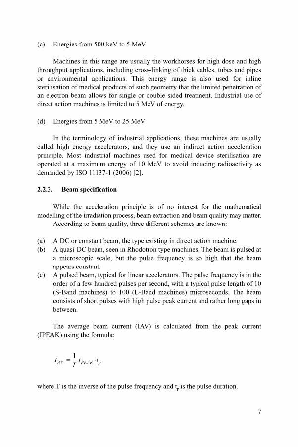
(c) A pulsed beam, typical for linear accelerators. The pulse frequency is in the order of a few hundred pulses per second, with a typical pulse length of 10 (S-Band machines) to 100 (L-Band machines) microseconds. The beam consists of short pulses with high pulse peak current and rather long gaps in between.

The average beam current (IAV) is calculated from the peak current (IPEAK) using the formula:

7

where T is the inverse of the pulse frequency and tp is the pulse duration.

IT

I tAV PEAK p= ◊1

For modelling purposes, DC and quasi-sc beam qualities are usually neglected in industrial irradiation, where the dose absorbed by a product matters. However, in pulsed beams, the number of pulses along the scan and scan frequency can matter, because these factors could introduce a non-uniform beam along a scan, which has to be taken into account in modelling.

The following describes the characteristics of scanned versus non-scanned beams. Non-scanned beams are common in low energy machines, where beam extraction occurs via a thin titanium foil, most often supported by a copper structure. While the microstructure of the cathode, window support and beam extraction foil are only considered in more demanding applications, the exact dose distribution measured along the exit window has to be known to achieve meaningful results.

Scanned beams are typical for high energy machines but can also be found in some low energy accelerators. The beam, when exiting the beam extraction window, can be:

— Parallel, in which case beam divergence is corrected with the help of a magnet;

— Divergent, with the beam symmetric to the beam axis;— Divergent, with an optional offset to the beam axis.

Figures 2–4 illustrate the different beam extraction topologies which are important in mathematical modelling.

In parallel beam topology, the divergent scanned beam is parallelized with the help of a magnet at the end of the scan horn. Figure 2 illustrates this topology for a horizontal beam line.

8

FIG. 2. Parallel beam.

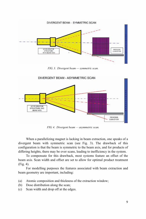
When a parallelizing magnet is lacking in beam extraction, one speaks of a divergent beam with symmetric scan (see Fig. 3). The drawback of this configuration is that the beam is symmetric to the beam axis, and for products of differing heights, there may be over scans, leading to inefficiency in the system.

To compensate for this drawback, most systems feature an offset of the beam axis. Scan width and offset are set to allow for optimal product treatment (Fig. 4).

FIG. 3. Divergent beam — symmetric scan.

FIG. 4. Divergent beam — asymmetric scan.

9

For modelling purposes the features associated with beam extraction and beam geometry are important, including:

(a) Atomic composition and thickness of the extraction window;(b) Dose distribution along the scan;(c) Scan width and drop off at the edges.

The atomic composition and thickness of the window are usually easy to discern, because only a thin foil (typically 40 m for high energy accelerators) is placed in the beam line.

Dose distribution along the scan is typically uniform, so modelling is easy. However special characteristics of scan function, such as humps at the end of a scan produced by double pulsing or non-uniform scan functions to shape dose distribution in a product, must be taken into account in the beam model.

Scan width is a very crucial parameter, when it enters into the calculation of absolute doses, because any loss due to over scan must be corrected by using a beam efficiency factor to prevent the wrong prediction of absolute doses. For this reason, the dose distribution measurement along the scan is an important piece of information which has to be carefully evaluated before any modelling can take place. Typically these studies are performed in the OQ (operational qualification) step of system commissioning.

2.3. PRODUCT HANDLING SYSTEMS

The term ‘product handling system’ usually stands for all modules which are associated with the conveyance of a product through the process. For a box or carrier based system, they include:

(a) A loading station where the product is loaded manually or automatically onto the product handling system;

(b) A bring-in section, which transports the product through the maze to the beam zone;

(c) The process or under beam conveyor;(d) Optional section which allows for turning of the beam before a second pass

in a double or multi-sided treatment scheme;(e) A removing section, which brings the product to the unloading station;(f) The unloading station.

Only in the case of industrial modelling purposes is the process or under beam conveyor of importance. The situation is rather simple for a box based system, while other treatment schemes may require much more elaborate

10

modelling.In a box or carrier based system the beam is either vertical (coming from the

top) or horizontal (coming from the side). Configuration may be much more complex in relation to other applications in the process. Some processes with special geometry include:

— Process chambers for flue gas treatment;— Spray or jets in water treatment;— Cross-linking of cables and wires;— Fluidized beds of grain, spices or polymer pellets.

For all applications, the distance between the exit window and the distance to product (DTP) are important in any modelling exercise.

While for high energy accelerators attenuation of the beam in air is usually negligible, beam fan out may have to be considered in divergent beams.

For low energy accelerators, DTP is an important process variable, which has to be carefully evaluated before modelling takes place.

The atomic composition and temperature of the gas gap between window and product are important at very low energies. Even small inhomogenities within the setup, such as dust particles on a thin foil, should be considered in more demanding applications.

2.4. PROCESS VARIABLES

The abstraction of the process model is condensed into process variables, which describe the irradiation process. This section briefly summarizes the process variables and discusses their importance in modelling.

Generally, variables are identified which control the process and make it predictable and reproducible. These process variables define the process framework. The actual numerical values of the process variables, called process parameters, define the process and provide a recipe for it.

In industrial irradiation, many process variables can be identified. Some are fixed attributes of a system, and remain the same from product to product.

The following process variables are important for modelling the radiation process. Other variables may matter more in special processes, but these have been ignored for the sake of simplicity.

A modelling procedure in the form of a written design document should include at least the following list:

— Beam energy;

11

— Scan width and scan distribution;— Distance to product;— Beam geometry.

2.4.1. Beam energy

Beam energy defines the penetration of a beam and hence the radiation field within the beam axis, because for most electron beam applications the dose contribution from bremsstrahlung is neglected. This is not true in systems with X ray converters, for which the radiation field is quite different, because only bremsstrahlung photons generate a dose to the product.

Beam energy may be considered monoenergetic, when the energy spread is very small (for example, 30 keV for a 10 MeV beam). Rhodotron type machines or systems with an energy discriminating magnet are examples of this.

Linear accelerators typically display a broad energy spectrum, meaning that the beam is composed of electrons with different energies. In most cases, the beam spectrum has an asymmetrical Gaussian distribution with a long tail towards low energies. Since some linacs do not know the energy spectrum well, it is a potential source of uncertainty in modelling.

2.4.2. Beam current

Beam current defines the number of electrons per second which penetrate the product or irradiation volume and hence the dose rate.

For modelling exercises in which only the dose distribution matters and no absolute dose values are required, the beam current is just a scaling factor and also does not matter. However, for any throughput and economic analysis, the beam current and its conversion to dose is important.

2.4.3. Product speed

Products are rarely irradiated in a static position. Static irradiation would generally only be used in the case of extremely high dose applications such as the colouring of gemstones, or for pallet treatments with low dose rate X ray beams.

Normally a product is moving through the beam zone and is thus irradiated. If the movement is uniform, as it is in most cases, process speed is a scaling factor which matters only in the calculation of absolute doses.

2.4.4. Scan width and scan distribution

12

In modelling, uniform illumination of the exit window by electrons is usually considered. If there is non-uniform dose distribution along the scan, it has to be evaluated and controlled, because it will have an impact on modelling results.

The actual extension of the scan, defined as scan width2 [3], applies to systems with a uniform scan, and is only a scaling factor used in calculations involving absolute doses.

The evaluation of beam utilization inefficiency introduced by dose drop-off at the end of a scan is a rather demanding dosimetry exercise. The usual industry practice is that a product is over scanned, so that it is only exposed to a uniform radiation field. The beam utilization factor is calculated by integrating the area under the measured scan distribution.

2.4.5. Distance to product

In any modelling exercise, the distance between the exit window and the scanned product should be evaluated and accounted for. Exceptions may be high energy electron beams, where small dose build-up in the air gap may be insignificant and does not matter.

2.4.6. Beam geometry

Beam geometry as discussed in Section 2.2.3. has to be evaluated for any impact on the radiation field. In many cases, simplifying to a parallel beam may be valid even in systems with a divergent beam, if the divergence is small and the product is sitting in the centre line of the scan.

2.4.7. Design specifications of an electron beam system

In this section, system design is summarized as a concise system specification checklist, which is then used in modelling.

2.4.8. System geometry and materials

As discussed earlier, only components in the vicinity of the radiation field are generally specified in the geometrical system description. These components may include:

— Beam exit window;

13

— Air gap;— Under beam conveyor system/process table;— Beam stopper;

2 See, for example, ISO/ASTM 51649:2005 for a definition and further discussion.

— Tray or carrier where the products sit;— Components which are close to the radiation field and which may provide

back scattering;— Irradiation cell walls, floor and ceiling.

The greatest modelling effort usually goes into the product itself. For simple geometries containing only rectangular layers or problems, for which only the dose distribution along the beam axis matters, this description may be easy.

For a fine grain description of a topologically complex product, a great deal of effort must to go into geometric description and its validation.

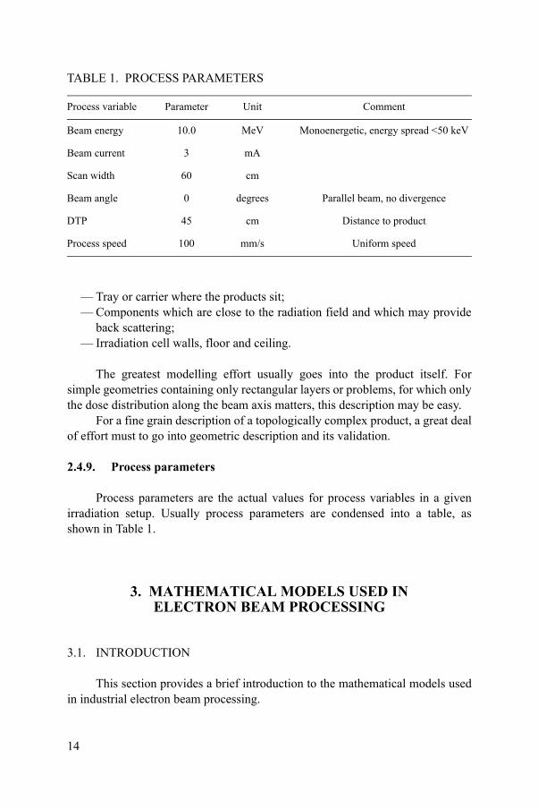
2.4.9. Process parameters

Process parameters are the actual values for process variables in a given irradiation setup. Usually process parameters are condensed into a table, as shown in Table 1.

3. MATHEMATICAL MODELS USED INELECTRON BEAM PROCESSING

TABLE 1. PROCESS PARAMETERS

Process variable Parameter Unit Comment

Beam energy 10.0 MeV Monoenergetic, energy spread <50 keV

Beam current 3 mA

Scan width 60 cm

Beam angle 0 degrees Parallel beam, no divergence

DTP 45 cm Distance to product

Process speed 100 mm/s Uniform speed

14

3.1. INTRODUCTION

This section provides a brief introduction to the mathematical models used in industrial electron beam processing.

Generally speaking, in radiation processing there is great interest in the dose deposited by ionizing radiation in the studied volume. This dose, correctly named energy dose (D = dE/dm), is responsible for the sterilizing and/or material modification effect which occurs in products. The variable dE is the mean incremental energy imparted by ionizing radiation to matter of incremental mass dm.

In electron beam processing, the source of ionizing radiation is a beam of accelerated electrons from an electron accelerator. Whereas dose is usually regarded as a macroscopic quantity in industrial processing, the volume of interest is a few cubic centimetres to cubic decimetres, and the agents of ionizing radiation are electrons, acting on an ultra-microscopic scale.

Therefore, any modelling of the irradiation process typically involves a mathematical description of the interaction of radiation in matter. The interaction of charged and neutral particles in matter is a highly developed and complex field which includes atomic, molecular, nuclear and high energy physics.

In the first half of the 20th century — when classical and quantum mechanical theories of ionization were developed — groundbreaking work was performed on the interaction of charged particles in matter. In parallel, the mathematical foundation of the passage of photons and neutrons in matter was developed and elaborated.

For industrial purposes, the description of radiation interaction with matter is limited to electrons and photons, as well as energies below 25 MeV. In medical physics, much higher energies (such as those existing in proton therapy) have to be considered; these complicate the analysis. Besides electrons and photons, neutrons, protons and ions have to be considered.

In high energy physics and space applications, where the impact of cosmic rays is calculated, the full spectrum of hadrons must also be part of the model.

There are very few energy applications or radiation detector simulations for which soft X rays and optical photons may have to be considered.

3.2. MATHEMATICAL MODELS OF IRRADIATION PROCESSING

This section provides a very brief overview of the physics of radiation transport in matter. Its purpose is to give a short introduction and to define terms

15

used in the following sections of the guide. It is not meant to be an in-depth tutorial on radiation physics, as there is already excellent literature available on this subject.

A classification of mathematical models for radiation processes is provided in ASTM 2232, Standard Guide for Selection and Use of Mathematical Methods for Calculating Absorbed Dose in Radiation Processing Applications [4]. This

document also provides an extensive list of references for mathematical modelling of radiation processing.

In this report, mathematical models are categorized into four different groups:

(a) Deterministic methods;(b) Semi-empirical models;(c) Empirical models;(d) Monte Carlo models.

3.2.1. Deterministic methods

The exact description of all possible interactions of particles in a radiation field is called radiation transport theory, which is a branch of statistical mechanics. The solution of the so called Boltzmann transport equations provides the expected fluence of radiation particles in matter.

However, solutions for electron beams are in general extremely complex and can only be solved analytically when simplifications and basic geometries are considered. Thus their impact on industrial radiation processing is virtually non-existent.

3.2.2. Semi-empirical methods

These models combine underlying theory with experimental dosimetry results to allow for dose distribution predictions in certain geometries, particularly for one dimensional problems or certain topologies.

While these models may be quite accurate in their field of applicability, care must be taken with any extrapolation.

3.2.3. Empirical methods

Empirical methods utilize relationships uncovered in experiments when making predictions regarding dose distribution for a limited number of setups and geometries. As for semi-empirical models, any extrapolation from the original domain of experimental verification could lead to wrong predictions.

16

3.2.4. Monte Carlo methods

In the Monte Carlo method, quantities of interest for the application are calculated through statistical sampling of interaction processes. The most important quantity will be absorbed dose for industrial applications, however,

dose rate, energy spectra, charge, fluence and fluence rate may also be of interest. For instance, the charge distribution absorbed in the mantle of a cable from electrons may be used to predict ruinous spiking.

Monte Carlo calculations are made via a statistical summary of individual radiation events, where state space variables such as energy, momentum and process angles are randomly sampled from appropriate probability density functions.

A Monte Carlo calculation therefore consists of running a large number of particle events until some acceptable statistical uncertainty of the desired calculated quantity has been reached. These individual events — calculated sequentially on a single CPU system or run in parallel on a CPU cluster — are usually called particle histories.

Statistical analysis of simulated events provides a clear picture and grants insight into what would occur in a real process.

One important aspect is that particle histories are considered to be independent and do not affect each other. This means we can ‘shoot’ electrons one after another, though in reality we bombard a target simultaneously with a huge number of electrons.3

The underlying probability functions of the process must be correct and match those of nature. Probability distribution functions (PDF) may be the outcome of an appropriate theory or model or be derived from experiments.

Supported by the availability of fast computers and highly developed software packages, Monte Carlo methods are the only ones used nowadays in electron beam processing. Therefore discussions about Monte Carlo methodology will be limited in the remaining sections of this guidebook.

3.3. INTERACTION OF PHOTONS WITH MATTER

3.3.1. Introduction

Photons play an important role in electron beam processing. Photons as quanta of electromagnetic radiation are uncharged and interact with matter using several mechanisms.

Before entering into a deeper discussion, a clarification of notations which

17

may confuse newcomers to the field is necessary: photons, X rays and gammas are the same physical objects, differing only in wavelength (and hence energy)

3 An electron beam of 1 mA consists of 6.25 1018 electrons.

and origin. The correlation between wavelength and energy is shown by the well known formula:

where E is photon energy, h is Planck’s constant, c is the speed of light and is the wavelength.

Electromagnetic quanta are generally called optical photons when their wavelength is between 1 and 1000 nm, which corresponds roughly to an energy amount of 1 eV to 1 keV.

Photons generated by the interaction of electrons with the Coulomb field of nuclei are called X rays. Photons which originate in nuclear reactions are called gammas.

3.3.2. Photo effect

The photoelectric effect is the most dominant process for low energy photons. A photon is fully absorbed by the electron of an atom; it is then boosted to a higher state or possibly rendered incapable of escaping the atom.

3.3.3. Compton scattering

Compton scattering can be seen as an inelastic interaction with the electron of an atom. Both the recoil photon and the electron have different momentum and energies after the interaction. Due to this fact, Compton scattering is also called incoherent scattering.

3.3.4. Pair production

Photons can interact in the field of a nucleus, annihilate, and produce an electron–positron pair. The photons’ energy must be higher than twice the remaining mass of the electron for this process to occur. Thus, pair production only takes place for photons with an energy of greater than approximately 1 MeV.

.h cE

18

3.3.5. Elastic scattering

Coherent or Raleigh scattering is elastic scattering; the photon does not change energy, only the direction is altered.

3.3.6. The concept of free path length

Determination of mean free path length or interaction length for a given process is crucial for the implementation of any Monte Carlo method. The mean free path length, which is a function of energy, is calculated as the inverse of the macroscopic cross-section [5]:

In this formula, ni stands for the number of atoms and is the cross-section of the element from which the material of interest is composed. Cross-sections per atom and mean free path lengths are usually calculated when a Monte Carlo package is initialized. From the mean path length, the next interaction point is calculated. The interaction probability per unit path length is 1/.

3.4. INTERACTION OF ELECTRONS WITH MATTER

3.4.1. Introduction

There are four process types in which electrons and positrons interact with matter, including: elastic collision, inelastic collision, bremsstrahlung emission and annihilation. These processes will be briefly clarified to provide a basic understanding of upcoming discussions.

3.4.2. Elastic scattering

In elastic scattering, electrons are diffracted at the Coulomb potential of the atoms and change their direction. There is practically no energy transfer and thus electron energy is preserved; the collision is elastic. The angular distribution of the deflected electrons is well understood.

3.4.3. Energy loss by ionization

ls

( )[ ( , )]

En Z Ei i

i

=◊Â1

19

When travelling through material, electrons excite (ionize) atoms along their path and lose energy. This is called inelastic scattering, because energy is transferred to the target. Their mass is equal to that of their interaction partners, the orbital electrons. Thus large deviations in electron paths are possible, and electrons may show erratic behaviour when travelling through matter.

3.4.4. Energy loss by bremsstrahlung

When electrons travel through matter and are deflected by the Coulomb potential of the nuclei they emit photons. This type of radiation is called bremsstrahlung. Bremsstrahlung production increases with electron energy and with the square of the atomic number Z.

3.4.5. Annihilation

Positrons may be generated by two processes: production of e+ e– pairs through high energy photons or through positron decay of a radionuclide. Positrons lose energy quite rapidly and are subsequently annihilated by electrons nearly at the same spot where they were generated. The remaining electron and photon masses are transformed into two photons, each with an energy of 0.511 MeV.

3.4.6. Monte Carlo simulation of electron interaction

Compared to photons, electrons interact heavily in matter and slow down through many collisions, each of which transfers little energy. On average, electrons only lose 30 eV per collision, so a 10 MeV electron interacts about 300 000 times in matter before its energy is exhausted [6]. Thus it is easy to understand that a detailed simulation of each interaction along its path is only possible at very low energies or with very thin foils, otherwise the required computation time would rise beyond practical limits.

It was the groundbreaking work of Martin Berger, from NIST [7], who introduced the notation and algorithms to perform condensed simulations’, in which only snapshots in particle history are considered. Such class I simulations work well both for high energies and thick media.

The combination of both strategies is called ‘class II simulations’, in which ‘hard events’ are simulated in detail and continuous energy loss is described using concentrated histories. There are detailed discussions of these advanced concepts existing in literature [8].

20

4. THE MONTE CARLO METHOD

4.1. INTRODUCTION

A brief introduction to the principles of the Monte Carlo method is given here. Since there are several extensive and excellent textbooks and tutorials available, this discussion will only present the material necessary to understand the following sections.

4.1.1. The Monte Carlo method — An introductory example

The following example is widely used in Monte Carlo literature to introduce the concept. Because it is so simple and enlightening, it is repeated here. More extensive discussions may be found in the literature [9].

Consider the following algorithm:

Step 1:

Choose a random number xi between 0 and 1. This random number marks a point on the x axis.

Step 2:

Calculate the associated y coordinate yi, which lies on a circle with xi as the x coordinate

Step 3:

Choose a random number, ri, in the interval [0,1]. Check whether this random number is less than or equal to yi. If ri yi then the point (xi, ri) lies within the area of the circle: this event is called a hit.

21i iy x

21

Step 4:

The repetition of this sequence many times clearly ‘paints’ or ‘probes’ the area with random points, and it is obvious that for a large number of events the quotient of the area under the circle and the total area equals the number of hits divided by the total number of events.

Since the area of the quarter circle is /4 and the total area is 1 in this case, it can be estimated that the number is

The following code fragment demonstrates this simple algorithm in Matlab [10]:

% Demonstrate Monte Carlo integration method:pi calculation

hit = 0;for i=1:1:10000

% Step 1: choose a random number in the interval [0,1]

x=random('Uniform',0,1,1,1);

% Step 2: calculate die y coordinate

y = sqrt(1-x^2);

% Step 3: choose a second random number in the interval [0,1]

r=random('Uniform',0,1,1,1); if (r < y)

A

A

Hits

EventsCircle

Total

= #

#

p = 4#

#

Hits

Events

22

hit = hit+1; end end pi_mc= 4*(hit/i)

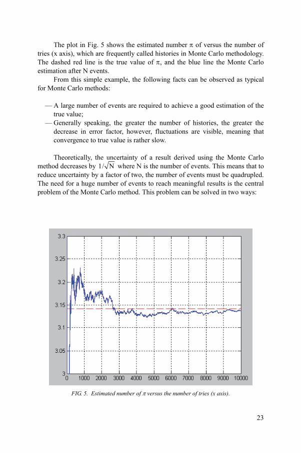
The plot in Fig. 5 shows the estimated number of versus the number of tries (x axis), which are frequently called histories in Monte Carlo methodology. The dashed red line is the true value of , and the blue line the Monte Carlo estimation after N events.

From this simple example, the following facts can be observed as typical for Monte Carlo methods:

— A large number of events are required to achieve a good estimation of the true value;

— Generally speaking, the greater the number of histories, the greater the decrease in error factor, however, fluctuations are visible, meaning that convergence to true value is rather slow.

Theoretically, the uncertainty of a result derived using the Monte Carlo method decreases by where N is the number of events. This means that to reduce uncertainty by a factor of two, the number of events must be quadrupled. The need for a huge number of events to reach meaningful results is the central problem of the Monte Carlo method. This problem can be solved in two ways:

1/ N

23

FIG. 5. Estimated number of versus the number of tries (x axis).

(a) ‘Brute force’ simulation, involving a very large number of events and a large number of CPU hours;

(b) ‘Variance reduction’ methods to decrease uncertainty in the volume of interest by directing simulation and increasing efficiency.

4.2. RANDOM NUMBERS

4.2.1. Introduction

By definition4 [11], a random number is a number generated by a process called a random number generator (RNG), the outcome of which is unpredictable, and which cannot be subsequently reliably reproduced. This process could be, for example radioactive decay; it cannot be predicted which nucleus is going to decay next.

For practical reasons, digital computers generate random numbers. Because — despite the sophistication of the algorithms — the sequence of random numbers generated will be repeated for a (very long) time, these software modules are called pseudo random number generators. Pseudo random numbers are studied in great detail in mathematics and computational sciences. A good overview with a focus on the Monte Carlo method is provided in Bielajew [12].

4.2.2. Pseudo random number generators

Most available pseudo random number generators produce uniform floating point random numbers or sequences of uniform random numbers in the interval [0.1]. ‘Uniformity’ in this context implies that probability is equal for each number in the interval. This is demonstrated in the following plot, which has been created by Matlab commands:

x=random('Uniform',0,1,1,1000000);hist(x,100)

One million random numbers are generated between 0 and 1, and a histogram with 100 bins is produced. The type of fluctuation which must be

24

tolerated when using finite statistics can be seen (Fig 6).

4 See, for example, http://www.randomnumbers.info/content/About.htm

In many cases, random numbers should be in the interval [a,b]. If rand() is the function used to generate a uniform random number in the interval [0,1], then rand()*(b-a)+a will generate a random number in the desired interval.

4.3. SAMPLING PROBABILITY DISTRIBUTION FUNCTIONS

Most numerical packages with the capability of including random number generation are also able to produce random numbers with other probability distributions, such as Gaussian or Poisson distributions. If the desired probability distribution is provided by the package, that implementation should definitely be used, because it is likely to be far more efficient than a self-coded algorithm.

In some cases it may be necessary to sample random numbers which follow

FIG. 6. Fluctuation when using finite statistics.

25

a specific probability density function p(x). There are two practical methods described in detail in literature [13]. This guidebook demonstrates methods using practical examples, leaving the further study of theory up to the reader.

4.3.1. Inversion method

The first method uses direct inversion of the cumulative probability distribution. The probability distribution function p(x) is considered in this case, with which the aim is to generate random numbers which follow this distribution function.

As a practical example, calculation of the interaction point of a photon along a path will now be discussed. The probability that a photon is not interacting is

p(x) = .e–x

where x is the coordinate along the path and is the interaction coefficient. The cumulative distribution function has been calculated using the inversion method, and the result is the integral of p(x).

This function is already normalized in the interval [0,], and can be mapped onto a random variable in the interval [0,1].

The key point is that this equation can be inverted analytically:

If r is a random number in the interval [0,1] then 1 – r is also a random number in the same interval. Thus, we can spare a subtraction and sample random

P x p x dx e xx

( ) ( )= = - -Ú ’ ’ 10

m

r P x e x= = - -( ) 1 m

e r

x r

x r

x- = -- = -

= - -

m

m

m

1

1

11

ln( )

ln( )

26

interaction points which follow the probability function p(x) with:

x r= - 1

mln( )

This is shown using a short Matlab code:

% sample random numbers which follow the probability function % p(x)= (1/u)*exp(-ux))

u= 10;r =random('Uniform',0,1,1,1000000);x= (-1/u)*log(r);hist(x,100)

One can see from Figs 7 and 8 that sampled interaction points follow the same distribution function as the original function.

27

FIG. 7. Sampled distribution.

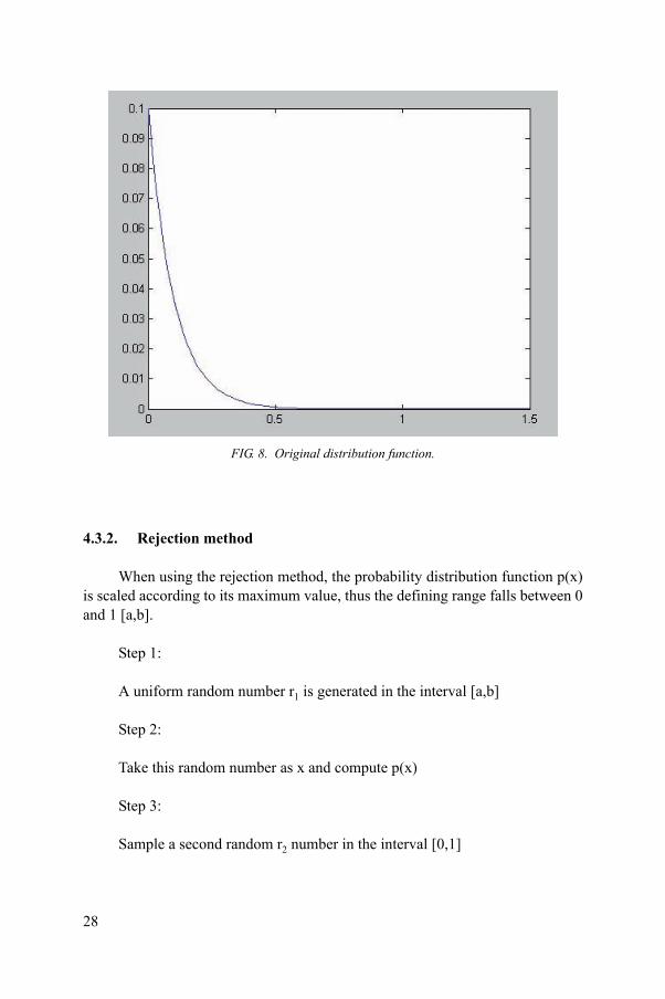
4.3.2. Rejection method

When using the rejection method, the probability distribution function p(x) is scaled according to its maximum value, thus the defining range falls between 0 and 1 [a,b].

Step 1:

A uniform random number r1 is generated in the interval [a,b]

Step 2:

FIG. 8. Original distribution function.

28

Take this random number as x and compute p(x)

Step 3:

Sample a second random r2 number in the interval [0,1]

Step 4:

If r2 < p(x) then accept x, if not, reject x

This method is very inefficient if pmax is much larger than the probability distribution mean, because many random numbers are wasted.

In literature many other algorithms, such as mixtures between inversion and rejection, are described. The average user of a Monte Carlo package will not be faced with the details of highly efficient implementation, because this is usually handled by the software package itself.

However, it is sometimes necessary to generate random numbers which follow the distribution in a histogram. This important topic will be addressed in the next section.

4.3.3. Sampling from a histogram

Probability distributions are often displayed as a histogram of experimental values. The inversion method can then be performed numerically, as is demonstrated by a simple example.

In simulating beams with non-monoenergetic energy distribution, the energy of an individual electron in a beam would have to be sampled where the energy distribution is known to be, for example, a type of Gaussian distribution with a mean of 10 MeV and a spread of about 1 MeV (Fig. 9).

29

FIG. 9. Experimental energy distribution.

In the next step, cumulative distribution is calculated, for example, using a spreadsheet program (Fig. 10).

The sampling algorithm itself is demonstrated in the following Matlab code fragment, where the cumulative probability distribution is condensed into 10 bins for a shorter code.

% Validation of generation of random numbers following a given % probability distributionekins=zeros(1,10);

bins=[0.000164,0.004759,0.059553,0.298724,0.693321,0.937691,0.994879,0.999857,0.999995,1];

energies = [9.0,9.25,9.5,9.75,10.0,10.25,10.5,10.75,11.0,11.25];for i=1:1:10000

FIG. 10. Cumulative distribution.

30

index = 1; x=random('Uniform',0,1,1,1); while(x > bins(index)) index= index+1; end

ekins(i) = energies(index);endhist(ekins,energies,10)

The basic ingredients of the algorithm are two arrays, one containing the cumulative probability distribution (array bins) and the other the associated energies (array energies).

In this simple algorithm, a random number x is picked and the associated E value is sought by walking through the bins (Fig. 11).

This numerical inversion of the function provides an energy value which is based on distribution according to the input energy distribution function. A histogram of 10 000 sampled events proves the assumption (Fig. 12).

This simple algorithm illustrates the basic principle and must be optimized in real world implementations to ensure accuracy and efficiency.

Using the same procedure, non-uniform scanning distributions can be simulated.

31

FIG. 11. Cumulative distribution.

5. MONTE CARLO TRANSPORT CODES

5.1. INTRODUCTION

As discussed before, when it comes to model electron beam applications, the user will most likely pick Monte Carlo transport codes, because they are widely available and other methods do not work well for electron beams.

A large number of different codes are available, and it may be quite difficult for a newcomer to pick the code which best suites a problem, as according to their skill level and experience.

FIG. 12. Histogram of 10 000 sampled events.

32

To address this problem, a lot of effort has been spent on surveying existing codes and classification schemes according to different parameters such as fields of application, ease of use, or required software skills.

A survey of the Panel of Gamma and Electron Beam Irradiation [14] provides a fairly detailed overview of six major Monte Carlo models and classifies them according to key features, such as:

— Availability;— Licensing;— Technical support;— Documentation;— Examples and training;— Prerequisites;— Technical code details;— Data input and output.

This document is the revised version of a lengthy document entitled Review of Monte Carlo and Deterministic Codes in Radiation Protection and Dosimetry, which was issued under a European Commission grant by the National Physical Laboratory (NPL) [15].

Different codes will be addressed after a summary of some radiation applications in which Monte Carlo codes are used.

5.2. MONTE CARLO TRANSPORT CODE APPLICATIONS

Monte Carlo transport codes are widely used in fields besides industrial radiation processing, and one can argue that industry can greatly benefit from developments in other fields.

This section provides a brief overview of some areas in which Monte Carlo radiation transport codes are used, including particular fields of focus. This allows for the categorization of some of the available codes based on special requirements from each field.

5.2.1. Medical applications

Medical applications rely heavily on Monte Carlo techniques; some of them are the most demanding applications of radiation transport codes. They are used, for example, for patient treatment planning, as well as in medical equipment design and validation.

These applications have some common aspects: first, they revolve around calculating doses in sometimes small and defined areas with high accuracy and

33

resolution. Dose calculation involves the computation of deposited energy in a chosen mass element in the form of absolute numbers, so the fundamental ingredients of Monte Carlo codes — like cross-sections — must be implemented with high accuracy.

As well, medical applications usually require very high resolution of an irradiation phantom in order to compare computations with, for example,

computer tomography (CT) data. This requires efficient memory handling, sophisticated graphic 3-D voxel algorithms and interfaces to commercial graphics packages.

A third fundamental requirement is the verification and validation of codes and the results generated using these codes. This will be discussed in more detail in a forthcoming section; historically some codes have a more detailed track record for being used in and suitable for medical applications.

Medical applications are a good example of the synergetic effects between radiation dosimetry and mathematical modelling. Without highly developed dosimetry, the validation and verification of mathematical models would not be possible. Mathematical models can save an enormous amount of resources, because they can assess systematic uncertainty by answering ‘when–if’ questions.

5.2.2. Radiation protection and shielding calculation

Other important Monte Carlo transport code applications are calculations associated with radiation protection and shielding design.

Several fundamental requirements originate from these applications. The first is linked to the number of simulated events, calculation speed and variance reduction.

As discussed briefly in Section 2.1.3, the required attenuation of radiation is in the order of 10 decades (from kGy per second to 1 Sv/h), and therefore in a brute force simulation only 1 of 1010 particles can make it from the radiation source to the protected area outside the shield. This provides an idea of simulation statistics and the absolute need for event biasing methods (see Section 5.13) to focus simulation on the volume in question.

Another requirement for Monte Carlo simulation is the ability to generate neutrons and track them correctly, because neutron flux can constitute a severe problem in radiation protection at higher energies.

This is linked to the general capability to simulate photonuclear reactions or high energy proton or ion beams as they are used in cyclotrons for the production of radiopharmaceuticals or proton therapy. In this case, the amount of radioactive isotopes and resulting activity can be predicted using Monte Carlo tools.

Even in industrial irradiation, photonuclear processes must be considered

34

when electron energy is above 10 MeV or the electron beam (greater than 5 MeV) is converted into X rays using a target. The requirement for assessment under these circumstances is clarified in ISO 11137:2006 [16] and may trigger more modelling in this area.

5.2.3. Space applications

Space applications have historically been a perfect playground for mathematical modelling because of the difficulty in undertaking dosimetry during space missions. Space applications include the study of material effects from ionizing radiation and the dose received by astronauts and equipment during a space mission.

One special requirement for space application modelling tools is the extension of models to very high energies, since these are frequently present in cosmic rays. Besides this, the capability of tracking particles in the presence of the earth’s magnetic field is mandatory.

Monte Carlo modelling techniques have benefitted from the space applications community, because powerful institutions are involved in modelling projects, and a lot of effort has gone into interface technology and add-on modules for Monte Carlo transport codes.

5.2.4. High energy physics

High energy physics has always been a driver behind using Monte Carlo methods in science and the name of one important code — GEANT (Generation and Tracking) — derives from the simulation and tracking of high energy vents and scoring hits in a detector.

Important requirements for a Monte Carlo code which is to be applied in high energy physics include the capability to simulate subnuclear particles (for example, all hadrons) and to handle extremely complex detector structures.

5.2.5. Industrial applications

Monte Carlo calculations for industrial applications are generally somewhat less demanding than those for some of the previously discussed fields. However, almost all the elements of the other applications are needed, and — typical for industry — must be highly competitive in every aspect. The code should be capable of running on a typical PC or laptop (generally Windows based), it should be easy to use with modest training requirements and it should be very versatile because applications and setups frequently differ.

35

In addition, data handling for input (geometry and material specifications) and output (dose distributions) should be easy and efficient, with interfaces to commercial graphics and analysis software.

5.3. SURVEY OF CODES

The following survey of available Monte Carlo tools for radiation transport calculations is not meant to be complete or provide a thorough classification.

It can only serve as a quick overview and starting point for more research. The sequence of codes is purely alphabetic and does not indicate any ranking. A detailed survey of available radiation transport codes has been published by NPL (NPL96) and a revised survey of Monte Carlo codes was published by the Panel on Gamma & Electron Irradiation in May 2007 [17].

5.3.1. Code distribution

There are basically two sources for the distribution of Monte Carlo transport codes, if a package cannot be downloaded directly from a supplier’s webpage.

In Europe the OECD Nuclear Energy Agency (OECD/NEA) maintains a database of software in the nuclear field available on www.nea.fr/html/databank. This database also contains Monte Carlo Radiation transport codes such as ITS and MCNP. These codes are available free of charge for the 28 member states in Europe, North America and the Asia-Pacific region.

In the United States of America, the Radiation Safety Information Computational Centre (RSICC), www-rsicc.ornl.gov, serves as a repository of nuclear codes. Distribution restrictions may apply and there is a distribution charge.

5.3.2. EGSnrc and beam

The EGSnrc system, www.irs.inms.nrc.ca, developed at the Canadian National Research Council, is a Monte Carlo simulation package of coupled electron–photon transport. EGSnrc has its roots in EGS4, originally developed at the Stanford Linear Accelerator Centre (SLAC).

As mentioned before, EGSnrc is limited to electrons and photons, but the electron energy range of 1 keV to 10 GeV is huge, and electron and photon processes have been modelled in great detail. EGSnrc is frequently used in medical physics applications (radio therapy calculation). The system is well

36

documented and benchmarked intensively against experimental data.EGSncr is available for Unix/Linux and Windows, and requires coding be

done in MORTRAN. MORTRAN (the name comes from ‘macro processed into Fortran’) is an extension of Fortran which makes heavy use of macros to structure code.

Users interested in medical physics applications may want to consider the BEAMnrc system. BEAMnrc, which stands for ‘A Monte Carlo Simulation System for Modelling Radiotherapy Sources’, is a collection of stand alone packages based on EGSnrc which allow the simulation of radiotherapy sources, for example electron accelerators for medical applications. These modules are very flexible, so they may be also used in industrial applications.

EGSnrc can be downloaded from the EGSnrc web site and it is free for non-commercial applications.

5.3.3. PENELOPE

The PENELOPE code system (an acronym for ‘Penetration and Energy Loss of Positrons and Electrons’) simulates the coupled transport of electrons, positrons and photons in arbitrary materials for a wide energy range, from a few 100 eV to 1 GeV [18]. A geometry package, PENGEOM permits the generation of electron–photon showers in homogeneous bodies limited by quadratic surfaces, such as planes, spheres or cylinders. A detailed description of the system is published at the OECD/NEA Data Bank and RSICC.

PENELOPE is the physics engine for the GAMBET commercial program (www.fieldp.com) which integrates Monte Carlo radiation transport in its suite sophisticated finite-elements programs.

5.3.4. Integrated Tiger System (ITS)

The Integrated Tiger System of coupled electron–photon transport via Monte Carlo was one of the first codes to be heavily used in industrial radiation processing.

It basically consists of three modules:

— TIGER: the module for one dimensional problems. Because of its ease of use, this module was, and still is, widely used for the calculation of depth–dose curves;

— CYLTRAN: a code for cylinder–symmetric problems;— ACCEPT: a code for three dimensional problems.

37

ITS is available from the OECD/ NEA for Member States as the (outdated) version 3.0.

5.3.5. RT Office 2.0

RT Office (Radiation Technological Office) was developed by the Radiation Dynamic group of Kharkov National University, Ukraine, (www-rdg.univer.kharkov.ua) as a common shell for a set of tools to assist practitioners in various problems involving radiation processing using electron beams, X rays, and gamma rays.

The toolset consists of semi-empirical models for dose distributions and very efficient Monte Carlo programs for specialized geometries like stacks and tubes.

5.3.6. MCNPX

MCNPX is a general purpose Monte Carlo radiation transport code for modelling the interaction of radiation with a large variety of particles. MCNPX stands for Monte Carlo N-Particle eXtended and it is developed and maintained by Los Alamos National Laboratory.

MCNPX is written in Fortran 90 and is available for the Unix/Linux and Windows operating systems. The code is well suited to run on a cluster using MPI (Message Passing Interface). MCNPX is used for nuclear medicine, nuclear safeguards, accelerator applications, nuclear criticality, and industrial irradiation simulation. Because of its nuclear physics capabilities, it is well suited to study X ray induced activation in high energy beams.

5.3.7. GEANT4

GEANT4 is a toolkit for the simulation of the passage of particles through matter. Its areas of application include high energy, nuclear and accelerator physics, as well as studies in medical and space science. Two main reference papers for GEANT4 have been published: G4 — A Simulation Toolkit [19] and the GEANT4 Toolkit [20].

GEANT4 is a complete rewrite of the popular radiation transport code Geant3, which was heavily used in high energy physics and helped enormously in the detector design of various elementary particle physics experiments.

GEANT4 was, and still is, a remarkable software project. The Geant

38

Collaboration decided in the 1990s not to follow the Fortran development line, but rather to undertake a complete rewrite of software in the object oriented programming language C++.

GEANT4 is maintained by a very active collaboration (cern.ch/geant4) and has an impressive list of applications, excellent quality assurance procedures and extensive documentation.

GEANT4 is a toolkit, so there is no stand alone program which the user must feed with input parameters or scripts to craft his own application. In contrast to other packages, the user must write their own C++ to define the detector, the beam and the physics processes. Therefore GEANT4 is extremely flexible and allows, for example, a change of geometry during simulation. The cost of this flexibility is a rather steep learning curve, which is made somewhat easier through excellent tutorials (which are sometimes free, in contrast to other codes) and example codes.

GEANT4 is supported for Linux/Unix and Windows operating systems. The software can be downloaded free of charge — as long as the license statements are observed — from the GEANT4 web site as source code or precompiled libraries. The several releases per year follow a detailed release plan issued by the Collaboration.

5.4. BASIC MONTE CARLO CODE MODULES

Despite their diversity and variable complexity, Monte Carlo radiation transport codes display similar basic building blocks, as presented in Fig. 13.

The geometry and material description module is essential for any Monte Carlo application because it defines the material and its geometry, where simulation takes place. In addition, in many cases the user can define sensitive areas — usually called detectors — where quantities of interest, like energy deposition, are recorded.

The physics engine is the core of the Monte Carlo code. Typically, the user specifies the particle source, for example single electrons with a particular energy and direction, and the physics engine takes care of the physics processes, generation of secondaries, and tracking of particles through the concerned volume. Although this may sound simple, the physics engine is enormously complex. Part of the complexity comes from the sampling of interaction points

39

FIG. 13. Monte Carlo radiation transport code building blocks.

(Section 4 illustrates that electrons interact so heavily that it is nearly impossible to compute and track any collision), tracking of particles over boundaries and cut-offs in energy and range needed to stop the simulation.

The physics engine provides information about particle types, energies and momentum. In some Monte Carlo codes this information must be directly transformed into the quantity of interest, such as dose in a certain volume element or hit in a detector.

The output module is the user’s front end, providing a visualization of simulation results. While only energy losses in certain volume elements are reported in some implementations, other codes show two dimensional or three dimensional dose distributions, or provide an interface to analysis and visualization packages.

Radiation transport codes can be grouped into stand alone implementation, in which the user is communicating with an executable via data and scripts and application frameworks, where the user is able to add subroutines and functions to a framework of routines, which are then compiled into an executable.

While stand alone programs may be more suited for beginners or occasional users, they have difficulties handling any special user requirements concerning input geometry, radiation source, physics model or data output. Therefore, the most powerful Monte Carlo radiation transport codes follow the toolkit approach, in which the user is supplying subroutines or scripts, which are then compiled into a complete, executable program.

This flexibility has a price, because an external compiler is usually required, and because of the complexity involved in handling these compilers and linkers. In addition, some computer language skills are necessary.

5.5. GEOMETRY INPUT

The first user task when running a mathematical model is provision of a description of the irradiation setup, meaning the geometry of the objects in the area of interest and the materials involved. This may be simple for one dimensional problems, which in the past provided useful and extensive information and insight into radiation physics. These types of models are still very important for industry work and are usually the first point of contact for

40

newcomers, which will be discussed in detail in Section 7.1.In one dimensional models, particles only propagate in the beam direction,

which is usually defined as the x coordinate. One can consider the geometry to be a stack of plates with infinite y and z coordinates. The only geometry information required is beam direction depth and the material — along with its atomic

composition — in which the particles are tracked. This simple setup is perfectly suited to the study of depth–dose curves, when fringe effects are of no concern.

5.5.1. Data driven input using text files

One dimensional geometries require few parameters to outline a problem, so they are ideally suited for data driven input.

Data driven input itself can be performed in two ways: the ‘old’, but still powerful way is via text files which originate from old data cards, and the ‘new’ way is via an GUI (Graphical User Interface).

The advantages of data driven input via text files are:

Portability:

Text (ASCII) files can be stored and handled easily using simple editors, like the Windows Editor. They are usually portable and can thus migrate between different operating systems.

Reference and validation:

It is highly recommended that input files be stored for each modelling process, so that they can be used for referencing and tracking when problems occur, or when a certain experimental setup must be validated.

Editing:

If a similar problem occurs, a collection of appropriate input files exist which may be edited to prepare for the new task.

Figure 14 provides an example of the well known TIGER code for simple depth–dose distribution in Windows editor.

5.5.2. Data driven input by GUI

Users working with Windows are accustomed to providing input

41

information via a graphical user interface (GUI). Well made GUIs are mostly self-explanatory and new or occasional users are able to enter the required information correctly, without having to worry about syntax and appropriate text file formats. This sharply spikes the learning curve, and guarantees nearly immediate success.

FIG. 14. Example of the TIGER code for a simple depth–dose distribution in Windows Editor.

42

FIG. 15. GUI of ModeRTL.

Figures 15 and 16 are examples of very well done GUIs of ModeRTL (see Section 5.3.5), a stand alone program which simulates electrons and X rays in various materials and topologies.

The concept of data driven input using a GUI is very powerful and comfortable for specialized topologies and applications. It is, however, very difficult to beat the flexibility of input files for more universal frameworks.

FIG. 16. GUI of ModeRTL.

43

5.5.3. Programmatic input

For three dimensional problems, the defining geometry using text files can be extremely tedious if it has to be done manually.

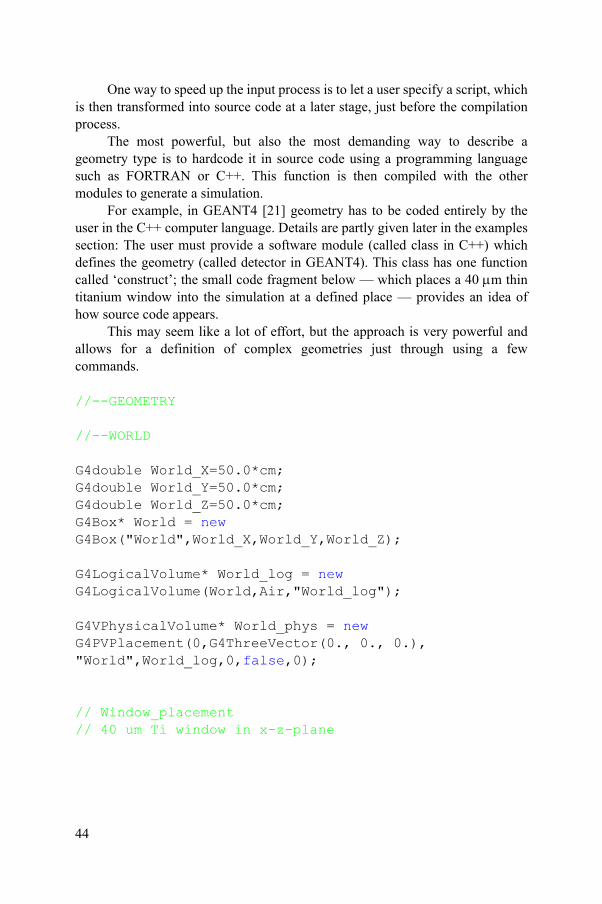
One way to speed up the input process is to let a user specify a script, which is then transformed into source code at a later stage, just before the compilation process.

The most powerful, but also the most demanding way to describe a geometry type is to hardcode it in source code using a programming language such as FORTRAN or C++. This function is then compiled with the other modules to generate a simulation.

For example, in GEANT4 [21] geometry has to be coded entirely by the user in the C++ computer language. Details are partly given later in the examples section: The user must provide a software module (called class in C++) which defines the geometry (called detector in GEANT4). This class has one function called ‘construct’; the small code fragment below — which places a 40 m thin titanium window into the simulation at a defined place — provides an idea of how source code appears.

This may seem like a lot of effort, but the approach is very powerful and allows for a definition of complex geometries just through using a few commands.

//--GEOMETRY

//--WORLD

G4double World_X=50.0*cm;G4double World_Y=50.0*cm;G4double World_Z=50.0*cm;G4Box* World = new G4Box("World",World_X,World_Y,World_Z);

G4LogicalVolume* World_log = new G4LogicalVolume(World,Air,"World_log");

G4VPhysicalVolume* World_phys = new G4PVPlacement(0,G4ThreeVector(0., 0., 0.), "World",World_log,0,false,0);

44

// Window_placement// 40 um Ti window in x-z-plane

G4double placeWindow_X= -35.0*cm;G4double placeWindow_Y= 0.0*cm;G4double placeWindow_Z= 0.0*cm;

G4Box* BeamExitWindow = new G4Box("BeamExitWindow",0.02*mm,30.0*cm,40.0*cm);// 40 um Titanium Window in z-y-planeG4LogicalVolume* BeamExitWindow_log = new G4LogicalVolume(BeamExitWindow,Titanium,"BeamExitWindow_log");G4VPhysicalVolume* BeamExitWindow_phys = new G4PVPlacement(0,G4ThreeVector(placeWindow_X,placeWindow_Y,placeWindow_Z),"BeamExitWindow",BeamExitWindow_log,World_phys,false,1);

It is evident that there are several features worth noting in the source code:

Parameters as variables

Geometry attributes such as position or length, as well as the width and height of objects, are stored as variables. Data types such as G4double are particular to GEANT4, which allows for portability between different platforms and computer hardware. Since the parameters are variables, they can be manipulated by C++ commands and constructs.

Units

Variables in GEANT4 not only have values, but also units. Many units are predefined, but the user can create his own based on need. This scheme ensures better readability and fewer data entry errors compared to packages which only allow one unit (for example, cm). To understand this better, look at the following line of C++ code:

G4Box("BeamExitWindow",0.02*mm,30.0*cm,40.0*cm);

45

World

The world is the mother volume of the simulation, where everything takes place. Particles are tracked only inside this mother volume and any other objects must be located in this world.

Solids

GEANT4 comes with a collection of predefined solids, for example, the rectangular G4box in the above example. Other CSG (constructed solid geometry) objects include cylinders, spheres or cones. Boolean operations (intersection, union and subtraction) may be performed on solid objects to generate new solids.

Logical volumes

Solids like ‘BeamExitWindow’ are expressed purely as geometrical objects, there is no information on the material the object is made of. This further step is accomplished by the definition of LogicalVolumes. In the example below, the object BeamExitWindow_log is associated with the element titanium, which was defined before:

G4LogicalVolume* BeamExitWindow_log = new G4LogicalVolume(BeamExitWindow,Titanium,"BeamExitWindow_log");

Physical volumes

Logical volumes have dimension and material; physical volumes, additionally, have information on the position of an object. In the example provided, the logical volume BeamExitWindow_log is placed at a certain position in the mother volume. It then becomes a physical volume.

This approach sounds complicated and exaggerated for simple geometries, but its real beauty is revealed when more complex geometries are considered. Logical volumes can be placed many times, and can be translated and rotated programmatically with only a few lines of source code.

5.5.4. CAD interface

The most elegant way to import the geometry of an object is as a CAD file. In addition to the object’s geometrical information, its materials have to be

46

defined and the CAD object must be placed in the desired position in the beam line.

These requirements make the CAD interface, which looks simple in principle, quite complex in reality. Several efforts are under way to automate the geometry input, but this field is still largely under development and new achievements may arise in the near future.

5.6. MATERIAL DEFINITION

For any radiation transport code, it is crucial to know the exact atomic composition of the material on which the simulation takes place. The definition is again made in three ways, as is evident from the geometry definition: text files, GUI and coding in a high level language.

Two characteristics of the material to be defined are absolutely required: atomic composition and density.

For elements, the definition is very simple: in most packages symbolic names from the periodic table of elements are recognized. Only the symbol name must be entered as seen in the example from an ITS 3.0 XGEN input file below: the first material below, aluminium, is defined and left at its built-in density. The second material, titanium, requires its density to be set to 4.54 g/cm3.

MATERIAL ALMATERIAL Ti WINDOW DENSITY 4.54

If the material is a molecule or compound material, then its definition may be slightly more complex. ITS 3.0 will be used again as an example. The gas is a simplified air, with 77.8% nitrogen and 22.2% oxygen. Its density is 0.001205 g/cm3.

MATERIAL GAS N 0.778 O 0.222 DENSITY 0.001205

If the chemical formula is known, it is very simple to calculate atomic composition. Polyethylene (PE), for example, has the chemical formula (H4C2)n. The atomic weight of hydrogen is 1.008 g/mole, that of carbon is 12.011 g/mole. The total atomic weight of H4C2 is 4 × 1.008 plus 2 × 12.011 = 28.054 g/mole.

To calculate the percentage of hydrogen, 4 times 1.008 is divided by total atomic weight, resulting in 14.37%. An equivalent calculation leads to 85.63% carbon. Thus, the atomic composition of PE is shown in Table 2.

TABLE 2. ATOMIC COMPOSITION OF PE

47

Polymer Hydrogen (%) Carbon (%)

H4C2 14.37 85.63

In GEANT4, the material definition is again programmatic. The following source code fragment in C++ provides an idea of how materials are defined. The first statement defines the element hydrogen:

G4Element* elementH = new G4Element("Hydrogen","H", 1., 1.00794*g/mole);

The following lines define polyethylene using the symbolic name PE. The first line provides density and defines PE as two components. In contrast to some other codes, GEANT4 allows a definition of the state of the material, kStatesolidin this example, as well as the temperature and the atmospheric pressure. The following two statements (AddElement method) define the atomic composition of the material known as PE.

G4Material* PE = new G4Material("PE", 0.94*g/cm3, 2,kStateSolid, 273.15*kelvin, 1.0*atmosphere);PE->AddElement(elementC,85.63*perCent);PE->AddElement(elementH,14.37*perCent);

The atomic composition of many materials used in modelling and dosimetry are easily found through the NIST ESTAR database at http://physics.nist.gov/PhysRefData/Star/Text/ESTAR.html. This program interactively calculates the stopping power of electrons, and as a by product displays the compound of many materials. PE, for example, is defined as in Fig. 17.

48

FIG. 17. ESTAR database of NIST.

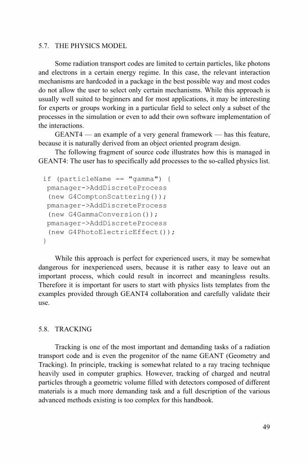
5.7. THE PHYSICS MODEL

Some radiation transport codes are limited to certain particles, like photons and electrons in a certain energy regime. In this case, the relevant interaction mechanisms are hardcoded in a package in the best possible way and most codes do not allow the user to select only certain mechanisms. While this approach is usually well suited to beginners and for most applications, it may be interesting for experts or groups working in a particular field to select only a subset of the processes in the simulation or even to add their own software implementation of the interactions.

GEANT4 — an example of a very general framework — has this feature, because it is naturally derived from an object oriented program design.

The following fragment of source code illustrates how this is managed in GEANT4: The user has to specifically add processes to the so-called physics list.

if (particleName == "gamma") { pmanager->AddDiscreteProcess (new G4ComptonScattering()); pmanager->AddDiscreteProcess (new G4GammaConversion()); pmanager->AddDiscreteProcess (new G4PhotoElectricEffect()); }

While this approach is perfect for experienced users, it may be somewhat dangerous for inexperienced users, because it is rather easy to leave out an important process, which could result in incorrect and meaningless results. Therefore it is important for users to start with physics lists templates from the examples provided through GEANT4 collaboration and carefully validate their use.

5.8. TRACKING

Tracking is one of the most important and demanding tasks of a radiation

49

transport code and is even the progenitor of the name GEANT (Geometry and Tracking). In principle, tracking is somewhat related to a ray tracing technique heavily used in computer graphics. However, tracking of charged and neutral particles through a geometric volume filled with detectors composed of different materials is a much more demanding task and a full description of the various advanced methods existing is too complex for this handbook.

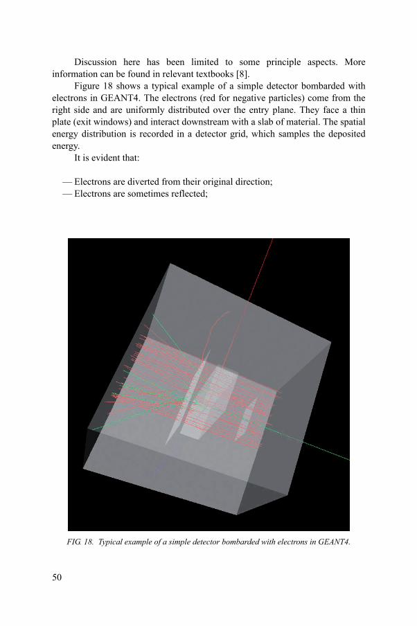
Discussion here has been limited to some principle aspects. More information can be found in relevant textbooks [8].

Figure 18 shows a typical example of a simple detector bombarded with electrons in GEANT4. The electrons (red for negative particles) come from the right side and are uniformly distributed over the entry plane. They face a thin plate (exit windows) and interact downstream with a slab of material. The spatial energy distribution is recorded in a detector grid, which samples the deposited energy.

It is evident that:

— Electrons are diverted from their original direction;— Electrons are sometimes reflected;

50

FIG. 18. Typical example of a simple detector bombarded with electrons in GEANT4.

— Secondary electrons are created;— Bremsstrahlung photons are generated (neutral particles are coloured

green).

The challenge in producing a radiation transport code lies in various areas: Electrons as charged particles interact so heavily that it is computationally not feasible to continuously simulate all their interactions and energy loss along their trajectory. The simulation has to advance in steps to keep the computational overhead manageable. The step size has to be adjusted according to factors such as material, interaction probability and user defined required accuracy.

Special attention must be given to boundaries when tracks are leaving one medium and entering another medium with a different atomic composition.

Figure 19 illustrates a typical tracking exercise, in which crosses mark points along the trajectory where simulation is updated.

51

FIG. 19. Tracking exercise (reproduced courtesy of Alex F. Bilajew).

5.9. CUT-OFFS

This leads to the definition of cut-off parameters. Since we know that a simulation has to advance in discrete steps, there are certain cut-off parameters necessary to steer a simulation.

Many transport codes implement an energy cut-off parameter, which defines in principle to which minimum energy a particle is tracked. If a particle has less energy than the cut-off energy, the remaining energy is dumped at the last step position. GEANT4 works with cuts in range and these can be specified by the user.

Regarding the validation of mathematical modelling, it is important to try different energy cuts and examine at which cut-off parameters results converge. This is important in order not to introduce a bias due to a cut-off parameter that is too large.

Figure 20 shows the depth–dose curve generated using two cut-off parameters. The high cut-off is 0.01 mm, the low cut-off is 0.0001 mm, a factor of 100 lower. The plot shows that in the tail of the depth–dose distribution (which is important for energy determination) the two curves overlap. In the buildup region small differences in the distribution are visible.

52

FIG. 20. Depth–dose curve generated with two cut-off parameters on GEANT4.

To summarize: cut-off parameters are necessary to make a numerical simulation of the radiation transport possible. However they have to be well understood and carefully handled in order to get correct and meaningful results.

5.10. DETECTORS AND HITS

Detectors in radiation transport codes resemble their physical counterparts and are regions in which physical quantities can be calculated and monitored. In many codes any volume serves as a detector; in GEANT4 for instance, a volume must be specified to act as a detector.

The most important quantity for industrial radiation processing is deposited energy, which leads to dose, the ultimate quantity of interest for many applications. In some applications, however, the deposited charge may also be of interest. An example is the cross-linking of cables, where charge buildup by absorbed primary electrons in the mantle may lead to discharge and insulation problems.

Figure 21 shows the simplified algorithms to calculate deposited energy in a detector cell. All particle tracks are followed and the deposited energy, Ei of the ith track in the detector, is calculated and accumulated.

The total energy stored in a detector cell is the sum of all tracks (index i) and all events (index j).

The scoring mechanism of the interesting physical variables is performed differently in various codes. MCNPX, for instance, uses the tally concept, with which predefined schemes can be chosen from an extensive tally list which generates all forms of 2-D and 3-D distributions (mcnpx.lanl.gov).

In GEANT4, scoring is also very versatile and introduces the concept of hits. According to GEANT4, a hit is a snapshot of the physical interaction of a track in the sensitive region of a detector.

Later versions of GEANT4 (starting from 8.1) feature ‘scorer’ objects,

( )N n

i jj i

E E

53

which facilitate the determination of deposited energy or dose enormously. An example is the scorer G4PSDoseDeposit, which uses geometry and material information to calculate dose in a detector cell.

Additional filters may be applied which take, for example, only charged or neutral particles into account. Therefore it is possible to calculate only the electron dose in a certain region.

5.11. FROM ENERGY DEPOSITION TO DOSE

In general, the output of mathematical models is the deposition of particle energy in a certain volume, usually referred to as the detector. This energy deposition (in eV or MeV) must be converted into a dose in kGy to provide meaningful information for the industrial irradiation process.

FIG. 21. Simplified algorithms to calculate deposited energy in a detector cell.

54

The conversion factors are simple and straightforward, and they are necessary for any real life application. For this reason, elaboration of conversion factors is presented in greater detail.

5.11.1. Conversion from energy deposition per unit area per electron

Many Monte Carlo packages, such as the ITS Tiger code, report energy deposition in MeV per unit area per electron. The formulas required to translate this quantity into a dose in kGy in an irradiation setup with specific values for:

— Beam current, I— Scan width, s— Conveyor speed, v

are shown below.The energy of an electron beam (in J) is the product of beam power (in W)

and irradiation time t (in s). In more practical units, this equation reads:

(1)

Beam power is numerically equivalent to the product of the energy (in MeV) and beam current (in mA).

(2)

Energy can be expressed as the product of De (in MeV cm2/g) and area density (in g/ cm2).

De is referred to as the energy deposition per unit area density per incident electron

(3)

The area density or standardized depth is represented by z, which is defined as the product of the layer thickness or distance in beam direction x (in cm) and density (in g/cm3). This quantity is equivalent to the mass of the layer divided by irradiated area A.

(4)

[ ] [ ]. [ ]E kJ P kW t s

[ ] [ ]. [ ]. [ ]E kJ E M eV I m A t s

2 2[ / ] [ ] / [ / ]De MeVcm g dE MeV dz g cm

2 3 2[ / ] [ ]. [ / ] [ ] / [ ]z g cm x cm g cm m g A cm

55

Equation (2) can be rewritten as:

(5)2 2[ ] [ / ]. [ / ]. [ ]. [ ]eE kJ D MeVcm g z g cm I mA t s

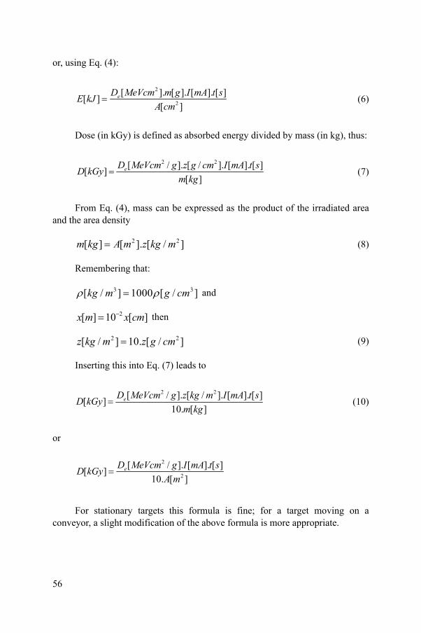
or, using Eq. (4):

(6)

Dose (in kGy) is defined as absorbed energy divided by mass (in kg), thus:

(7)

From Eq. (4), mass can be expressed as the product of the irradiated area and the area density

(8)

Remembering that:

and

then

(9)

Inserting this into Eq. (7) leads to

(10)

or

2

2

[ ]. [ ]. [ ]. [ ][ ]

[ ]eD MeVcm m g I mA t s

E kJA cm

2 2[ / ]. [ / ]. [ ]. [ ][ ]

[ ]eD MeVcm g z g cm I mA t s

D kGym kg

2 2[ ] [ ]. [ / ]m kg A m z kg m

3 3[ / ] 1000 [ / ]kg m g cm

2[ ] 10 [ ]x m x cm

2 2[ / ] 10. [ / ]z kg m z g cm

2 2[ / ]. [ / ]. [ ]. [ ][ ]

10. [ ]eD MeVcm g z kg m I mA t s

D kGym kg

2

2

[ / ]. [ ]. [ ][ ]

10. [ ]eD MeVcm g I mA t s

D kGyA m

56

For stationary targets this formula is fine; for a target moving on a conveyor, a slight modification of the above formula is more appropriate.

Irradiated area A is the product of scan width times the distance the product travels with constant conveyor speed v in unit time. Introducing the speed one gets:

(11)

Equation (11) implies that the product is catching 100% of the beam. To take into account realistic cases, in which some part of the beam is lost due to overscanning of a product, an efficiency factor (which is in the order of 0.9) is introduced. Equation (11) then reads as:

(12)

which is a well known formula in radiation physics [22].This formula is especially suitable for one dimensional problems, in which

dose is a function of the area density z. The output De(z) of a Monte Carlo program — for example its ITS — can be directly inserted in Eq. (10) to achieve a dose in kGy. Equation (12) is also useful when only the surface dose is of interest, such as in surface sterilization or film cross-linking applications. The reported stopping power at a given energy is inserted as De, and the absorbed dose is easily calculated for the given irradiation conditions. This calculation is only correct for materials and energies with small reflection coefficients.

5.12. UNCERTAINTY IN MONTE CARLO CALCULATIONS

In science, a measurement should have a value, a unit and an associated uncertainty. The presentation of mathematical modelling results should follow the same rules. However, this is still not common practice because of the intrinsic complexity of uncertainty evaluations.

Despite the fact that this problem cannot be fully discussed in this

2[ ]. [ ][ ]

10. [ ].v[ / ]eD MeVcm I mA

D kGys m m s

2[ ]. . [ ][ ]

10. [ ].v[ / ]eD MeVcm I mA

D kGys m m s

57

handbook, the sources of uncertainty will be briefly considered and analysed in a systematic way.

A generally accepted scheme is to categorize uncertainties into types A and B. Details can be found in the ISO Guide to the Expression of Uncertainty in Measurement [23].

By definition, type A uncertainty estimation is a method of evaluating uncertainty through the statistical analysis of a series of observations, whereas type B uncertainty evaluation is undertaken using other means.

5.12.1. Sources of uncertainties

The first task when evaluating uncertainties is to collect all possible sources through brainstorming (Fig. 22).

In this plot, four major sources of uncertainty are considered:

Geometry input uncertainty

A good geometry input is important, and a pre-requisite for successful modelling. Several sources of uncertainty may be associated with geometry input.

First, the details of a geometric model can matter. Since there is always a compromise between detail and effort, experience is required to determine which geometric detail is important for modelling. On the other hand, if any detail is implemented, it may blow up the application and result in unacceptable memory requirements and computing time.

Second, measurements have uncertainties which may affect a model. These uncertainties are of type A, because they can be addressed by several sets of geometry measurements.

58

FIG. 22. Brainstorming on possible sources of uncertainty.

In practice, the most critical problem is incorrect and erroneous data entry. This is particularly the case when large geometries and textual input are involved. This type B uncertainty can only be handled through verification and validation of the data entry process. Verification can be seen as a four eyes check of data, validation as reconstruction of the geometry using a CAD system and comparison with original geometry.

Simulation engine

Uncertainty sources in this area include the number of histories; this is addressed in more detail in the next paragraph. Cut-off parameters may bias the simulation and hence be a source of type B uncertainty.

Misuse of variance reduction procedures may influence the simulation negatively and contribute to uncertainty.

Physics model

Uncertainties associated with the physics model are incorrect cross-sections, software bugs in the implementation of processes, and the use of algorithms and approximation in inappropriate energy regimes. These are type B uncertainties and can only be addressed through experimental validation.

Data handling

Data handling is another source of uncertainty with may affect the quality of modelling results. Typical defects during data handling are software bugs in data manipulation, for example. in spreadsheet programs, or errors made when presenting results. Again these are type B uncertainties and can only be addressed through adequate software quality procedures and experimental validation.

5.12.2. Simulation statistics

The easiest source of uncertainty to manage is the limited statistic (number of events, histories) in a Monte Carlo simulation, which comes under type A.

The variance of a variable derived by Monte Carlo sampling follows 1/N,

59

where N is the number of events. This means that variance decreases when the number of events or histories increases. The plot in Fig. 23 provides an example of the variance reduction which can be achieved by increasing the number of events.

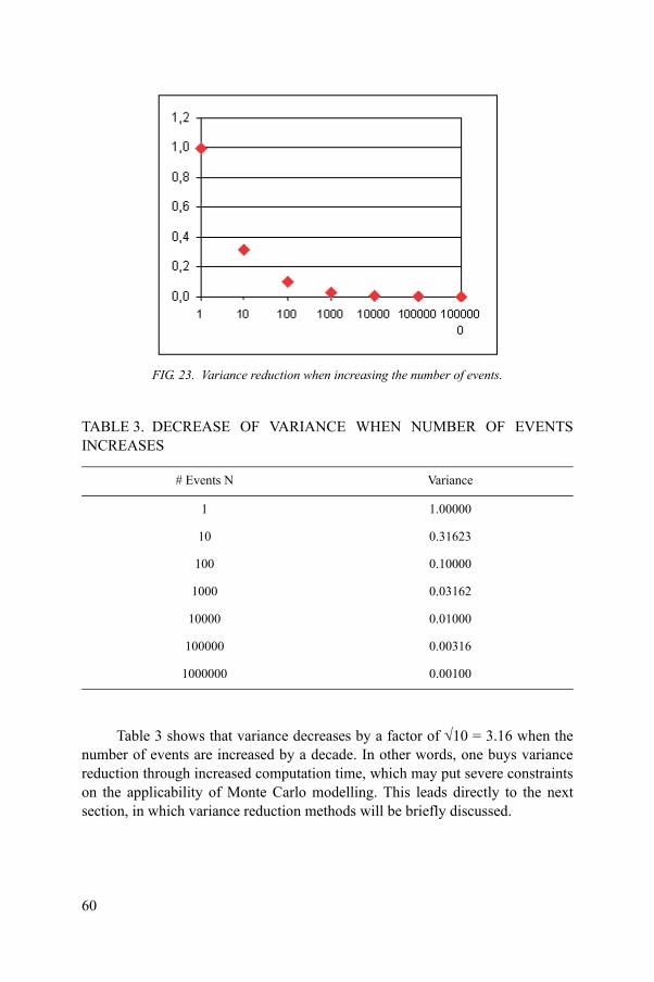
Table 3 shows that variance decreases by a factor of 10 = 3.16 when the

TABLE 3. DECREASE OF VARIANCE WHEN NUMBER OF EVENTS INCREASES

# Events N Variance

1 1.00000

10 0.31623

100 0.10000

1000 0.03162

10000 0.01000

100000 0.00316

1000000 0.00100

FIG. 23. Variance reduction when increasing the number of events.

60

number of events are increased by a decade. In other words, one buys variance reduction through increased computation time, which may put severe constraints on the applicability of Monte Carlo modelling. This leads directly to the next section, in which variance reduction methods will be briefly discussed.

Combining uncertainties needs to be undertaken separately for type A and type B uncertainties in quadrature, assuming the uncertainties are independent.

Assessment of type B uncertainties is much more difficult and beyond the scope of this discussion.

5.13. VARIANCE REDUCTION TECHNIQUES

Variance reduction techniques are used to make Monte Carlo calculations more efficient, which means that CPU time is spent in such a way that maximum information of interest can be retrieved from a program output.

To illustrate this point, the shielding problem must once again be considered. When bombarding a shield with electrons, the dose rate downstream is more important than the dose inside the shield. Hence one must steer or bias the program in such a way that more particle histories (photons) make it through the shield than are absorbed in the shielding material.

The biasing radiation transport for this type of problem may be the ‘exponential transform technique’. The probability distribution function (see Section 4.3.1)

for the next interaction point is biased by a factor, and this factor is used to weigh the event and compensate for the bias.

Another technique is known as ‘Russian roulette’. If a particle is travelling in a wrong direction and is likely to be lost for a detector of interest, it is discarded. The small chance that an event indeed makes it to the detector and scores is compensated by a survival probability.

Any variance reduction method must be applied with extreme care and requires skilled and experienced users.

2 2 21 2 ..A nu u u u

1ln( )x r

61

5.14. VERIFICATION AND VALIDATION

Mathematical modelling is a widely accepted method in radiation processing. As mentioned above, it is absolutely necessary to verify and validate a model before drawing any conclusions from its output.

The risk associated with using Monte Carlo results is linked to the effort which must go into the verification and validation processes. An extreme example is cancer treatment planning programmes, where the lives of patients are at stake.

The terms verification and validation are sometimes intermingled and difficult to separate. For this reason, the acronym V&V (for verification and validation) is often used when software quality issues are addressed.

In general, the verification of software means checking whether the software works ‘correctly’, meaning that no logical or mathematical defects have been introduced into the software.

Validation, on the other hand, is the process used to make sure a product serves its planned purpose and all user requirements are met.

Besides using well established methods of software quality for code production, benchmarking a code against experiments is essential. Benchmarking is defined as the comparison of a model to independent measurements or calculations under similar conditions using established criteria of uncertainty [24].

Monte Carlo codes generally have a large record of benchmark tests, especially those used in the medical field. Benchmarks are a part of validation because they demonstrate that a code can be successfully applied to a certain problem at a specific beam energy range.

The following plots are taken from the GEANT4 collaboration web page http://www.ge.infn.it/geant4/lowE/results/grafmuro.html; they document the validation of photon attenuation coefficients in water for various energies. Figure 24 presents a model output using the low energy extension of electromagnetic processes compared to NIST data. Figure 25 shows the deviation between data and the forecast of standard electromagnetic processes and their low energy extensions.

Before using a mathematical model, it is important to collect available benchmarks to define the validated domain (energy, particle type) of the model. If

62

the model is used in the validated domain, a high probability exists that model predictions are valid and mimic experimental results within the given uncertainty.

FIG. 24. Model output using the low energy extension of electromagnetic processes compared with NIST data

63

FIG. 25. Deviation between data and forecast of standard electromagnetic processes and their low energy extensions.

Intercomparison of dose distribution calculated using different codes and comparison with an experiment are also interesting for industrial applications, and increase confidence for the end user. This problem is addressed by the Radiation Process Simulation and Modelling User Group RPSMUG through benchmark tests with different codes for Rhodotron and linac type accelerators [25].

6. CALCULATIONS USING ONE DIMENSIONALMATHEMATICAL MODELLING

6.1. INTRODUCTION

This section provides some examples which demonstrate the use of one dimensional models in radiation processing. As a theoretical pre-requisite, depth–dose curves and energy determination in these plots are discussed. The concept of stopping power will be reviewed in an upcoming section, due to its importance when studying layered objects.

6.2. STOPPING POWER AND DEPTH–DOSE CURVES

When electrons travel through matter, they continuously lose energy along their path. This energy loss dE/dx is referred to as stopping power, measured in eV/cm. Two sources contribute to total stopping power:

(a) Collision stopping power: Average energy loss per unit path length through Coulomb scattering, which results in ionisation and excitation of atoms.

(b) Radiation stopping power: Average energy loss per unit path length through the emission of photons (bremsstrahlung).

When energy loss is divided by density, the mass stopping power is found, which is usually given in the unit MeV cm2/g.

64

1 dES

dx

The definitive source for calculating electron stopping power is the ESTAR program from NIST. The http://physics.nist.gov/PhysRefData/Star/Text/ ESTAR.html web site contains detailed reference information about stopping power calculations and measurements, as well as the interactive ESTAR program (Figs 26 and 27).

In dosimetry, collision stopping power is the relevant quantity, and its dependency on a material’s atomic composition is crucial for the interpretation of modelling results.

Table 4 presents the collision stopping power of different elements at various energies.

In dosimetry, absorbed doses are calculated and reported using water as the reference material. This ‘dose to water’ convention has its origin in medical physics and must be taken into account when dealing with other materials.

Table 5 provides the deviation of collision stopping power in percentage at 10 MeV from the reference element water.

There is little deviation (less than 5%) in polyethylene, tissue and air, however there is a big difference for metals (17% for aluminium and 26% for iron). This means that electrons lose more energy per unit length in metals, hence they deposit less energy in a metallic region.

65

FIG. 26. Example of ESTAR user iInterfac.

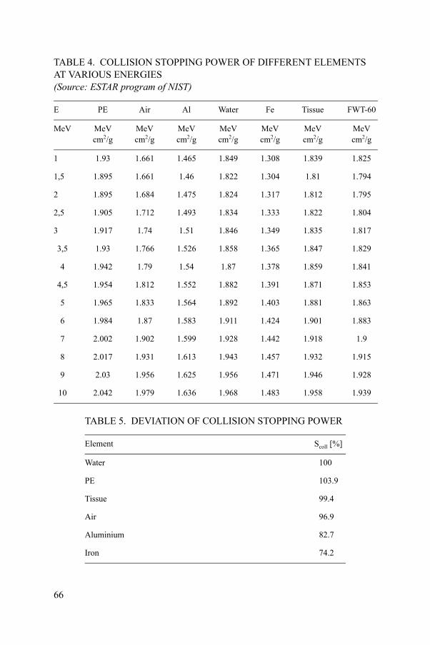
TABLE 4. COLLISION STOPPING POWER OF DIFFERENT ELEMENTS AT VARIOUS ENERGIES(Source: ESTAR program of NIST)

E PE Air Al Water Fe Tissue FWT-60

MeV MeVcm2/g

MeVcm2/g

MeVcm2/g

MeVcm2/g

MeVcm2/g

MeVcm2/g

MeVcm2/g

1 1.93 1.661 1.465 1.849 1.308 1.839 1.825

1,5 1.895 1.661 1.46 1.822 1.304 1.81 1.794

2 1.895 1.684 1.475 1.824 1.317 1.812 1.795

2,5 1.905 1.712 1.493 1.834 1.333 1.822 1.804

3 1.917 1.74 1.51 1.846 1.349 1.835 1.817

3,5 1.93 1.766 1.526 1.858 1.365 1.847 1.829

4 1.942 1.79 1.54 1.87 1.378 1.859 1.841

4,5 1.954 1.812 1.552 1.882 1.391 1.871 1.853

5 1.965 1.833 1.564 1.892 1.403 1.881 1.863

6 1.984 1.87 1.583 1.911 1.424 1.901 1.883

7 2.002 1.902 1.599 1.928 1.442 1.918 1.9

8 2.017 1.931 1.613 1.943 1.457 1.932 1.915

9 2.03 1.956 1.625 1.956 1.471 1.946 1.928

10 2.042 1.979 1.636 1.968 1.483 1.958 1.939

TABLE 5. DEVIATION OF COLLISION STOPPING POWER

Element Scoll [%]

Water 100

PE 103.9

66

Tissue 99.4

Air 96.9

Aluminium 82.7

Iron 74.2

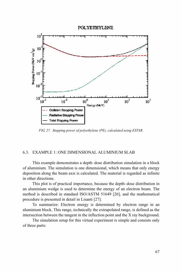
6.3. EXAMPLE 1: ONE DIMENSIONAL ALUMINIUM SLAB

This example demonstrates a depth–dose distribution simulation in a block of aluminium. The simulation is one dimensional, which means that only energy deposition along the beam axis is calculated. The material is regarded as infinite in other directions.

This plot is of practical importance, because the depth–dose distribution in an aluminium wedge is used to determine the energy of an electron beam. The method is described in standard ISO/ASTM 51649 [26], and the mathematical procedure is presented in detail in Lisanti [27].

To summarize: Electron energy is determined by electron range in an

FIG. 27. Stopping power of polyethylene (PE), calculated using ESTAR.

67

aluminium block. This range, technically the extrapolated range, is defined as the intersection between the tangent in the inflection point and the X ray background.

The simulation setup for this virtual experiment is simple and consists only of three parts:

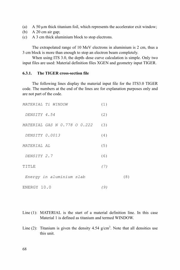
(a) A 50 m thick titanium foil, which represents the accelerator exit window;(b) A 20 cm air gap;(c) A 3 cm thick aluminium block to stop electrons.

The extrapolated range of 10 MeV electrons in aluminium is 2 cm, thus a 3 cm block is more than enough to stop an electron beam completely.

When using ITS 3.0, the depth–dose curve calculation is simple. Only two input files are used: Material definition files XGEN and geometry input TIGER.

6.3.1. The TIGER cross-section file

The following lines display the material input file for the ITS3.0 TIGER code. The numbers at the end of the lines are for explanation purposes only and are not part of the code.

MATERIAL Ti WINDOW (1)

DENSITY 4.54 (2)

MATERIAL GAS N 0.778 O 0.222 (3)

DENSITY 0.0013 (4)

MATERIAL AL (5)

DENSITY 2.7 (6)

TITLE (7)

Energy in aluminium slab (8)

ENERGY 10.0 (9)

68

Line (1): MATERIAL is the start of a material definition line. In this case Material 1 is defined as titanium and termed WINDOW.

Line (2): Titanium is given the density 4.54 g/cm3. Note that all densities use this unit.

Line (3): Material 2 is a gas (simplified air) made from 77.8% nitrogen and 22.2% oxygen.

Line (4): The gas is given the density 0.0013 g/cm3, which is approximately the standard density of air (= 1.293 kg/m3).

Line (5): Material 3 is defined as aluminium.

Line (6): Aluminium is given the density 2.7 g/cm3.

Line (7): The control word TITLE marks a title line, describing the project that is following.

Line (9): Electron energy is set to 10 MeV. Note that all energies are given in megaelectronvolts (MeV).

This file can be written in any text editor and must be saved under the name xgen in the INPUTS directory of the ITS3 folder.

This material file is used to calculate the necessary cross-sections for the simulations. The material numbers are important in the following geometry definition, so it is wise to make a printout for reference and cross-check material/geometry definition. Wrong input data is a major source of errors and careful validation is an important step in the software quality control process.

In the following ITS3 examples, ITS code is installed in the ITS3 directory. The following line in the command window will generate the cross-section files.

The MAKEXGEN program creates a file xgen in the OUTPUTS folder of ITS3. This file is then used by the TIGER simulation code (Fig. 28). It is a goodidea to check this file in an editor for any error messages during cross-section calculations.

69

FIG. 28. Makexgen program.

6.3.2. The TIGER geometry and simulation control file

The second file required is the TIGER geometry definition and simulation control file. Again, the numbers at the end of the lines are for explanation purposes only and are not part of the code.

ECHO 1

TITLE

...10 MeV Al TEST PROBLEM 50 um Ti-Window 20 cm air 3 cm Al in 60 bins for depth–dose validation

************************* GEOMETRY ********************************

* MATERIAL SUBZONES THICKNESS ELECTRON-CUTOFF FORCING

GEOMETRY 3 (1)

1 5 0.005 (2)

2 5 20 (3)

3 60 3 (4)

************************* SOURCE ********************************

ELECTRONS (5)

ENERGY 10.0 (6)

CUTOFFS 0.001 0.001 (7)

70

* DEFAULT DIRECTION

DIRECTION 0.0 (8)

************************* OUTPUT OPTIONS ************************

ELECTRON-ESCAPE

NBINE 2

NBINT 4

PHOTON-ESCAPE

NBINE 2

NBINT 4

************************* OTHER OPTIONS ***********************

* NO-COHERENT

* NO-INCOH-BINDING

HISTORIES 100000 (9)

BATCHES 100 (10)

Line (1) The geometry consists of 3 layers.

Line (2) Layer 1 is titanium (material 1); it consists of 5 bins and has an overall thickness of 50 m (0.005 cm).

Line (3) Layer 2 is air. It also consists of 5 bins and has an overall thickness of 20 cm.

Line (4) Layer 3, the aluminium slab, is divided into 60 bins and has an overall thickness of 3 cm. Thus, each subdivision in which energy deposition is calculated has a width of 0.5 mm.

71

Line (5) The particles are electrons.

Line (6) The particle has an energy of 10 MeV.

Line (7) The cut-off parameters are 0.001 MeV.

Line (8) Electron direction is along the x axis and enters the layers of material perpendicularly.

Lines (9, 10) 10 million events are calculated.

The commands shown in Fig. 29 use the above TIGER input file and calculate energy deposition in the defined geometry.

6.3.3. The TIGER output file

The output file tiger.out is located in the directory ITS3/outputs. It has a complex structure and contains a lot of information. For the average user, the only section of importance is that summarizing energy deposition. Another section which might be of interest is charge deposition, which is important, for example, in the study of cable irradiation.

There are numerous ways to extract information from the output file. One simple way is to open the file tiger.out with Excel. Use spaces as delimiters and ‘.’ as decimal separators (see Figs 30 and 31).

Dose information is found by scrolling down the file. The first lines of energy deposition are shown in Fig. 32. The energy deposition dE/dz (mass stopping power) is normalized to one source particle and given in MeV cm2/g.

For further analysis only a few columns are needed:

(1) Column 1 is the subzone number.

FIG. 29. Runits3 tiger tiger xgen command.

72

(2) Column 2 is the material number as defined in the xgen file. (3) The range of standardized depth is next (data columns 5 and 6); the first

columns mark the beginning of the subzone and the latter the end.It is a good idea to check subzone data through comparison with material and geometry input files:

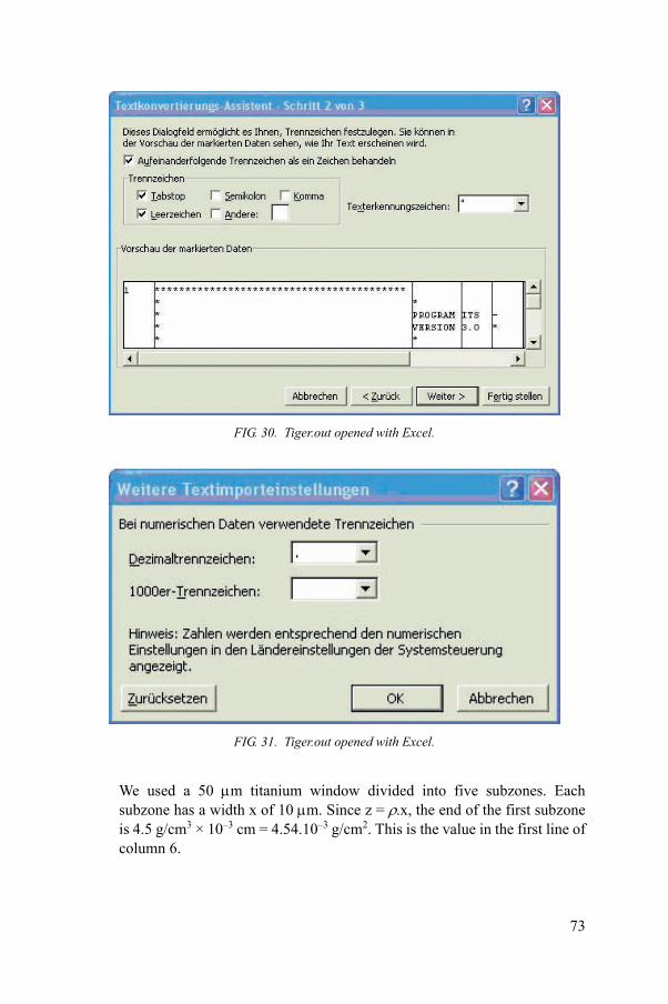
FIG. 30. Tiger.out opened with Excel.

FIG. 31. Tiger.out opened with Excel.

73

We used a 50 m titanium window divided into five subzones. Each subzone has a width x of 10 m. Since z = .x, the end of the first subzone is 4.5 g/cm3 × 10–3 cm = 4.54.10–3 g/cm2. This is the value in the first line of column 6.

(4) The energy deposition is in the next to last column. It is 1.2666 MeV cm2/g for our example.

6.3.4. Analysis of the output file

The following columns are a good start for further analysis of the file (see Fig. 33). Table 6 defines the variables used.

The first plot shows energy deposition along the full setup: titanium foil, air and aluminium (Fig. 34).

Titanium has a low energy deposition (because of its low stopping power), a rise in energy deposition per depth in air and the full stopping of the electrons in aluminium, occurring at about 2 cm. The buildup of the depth–dose curve is clearly seen; it comes from the energy deposition of secondary electrons.

TABLE 6. ANALYSIS OF THE OUTPUT FILE

zstart beginning of the subzone in g/cm2

zend end of the subzone in g/cm2

zavg average standardized depth of the subzone

xstart, xend, xavg depth of the subzone (beginning, end average) in cm relative to the material

x cul start, -end, -avg cumulative depth values in cm

dE/dz energy deposition in the subzone in MeV cm2/g

FIG. 32. Tiger.out opened with Excel.

74

The plot looks completely different if energy deposition is placed along the standardized depth z = x.r (Fig. 35). This figure shows that the titanium foil and the air gap are ‘insignificant’ for the electron beam, and that only the aluminium slab matters for energy deposition.

FIG. 33. Analysis of the output file.

75

FIG. 34. Energy deposition along the full setup.

FIG. 35. Energy deposition in aluminium.

76

FIG. 36. Energy deposition along standardized depth z = x.ρ.

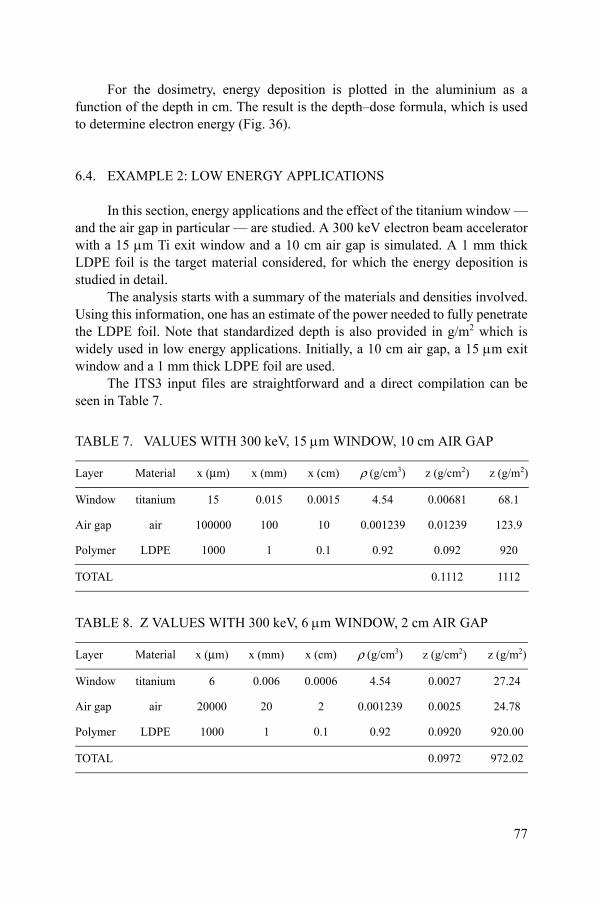
For the dosimetry, energy deposition is plotted in the aluminium as a function of the depth in cm. The result is the depth–dose formula, which is used to determine electron energy (Fig. 36).

6.4. EXAMPLE 2: LOW ENERGY APPLICATIONS

In this section, energy applications and the effect of the titanium window — and the air gap in particular — are studied. A 300 keV electron beam accelerator with a 15 m Ti exit window and a 10 cm air gap is simulated. A 1 mm thick LDPE foil is the target material considered, for which the energy deposition is studied in detail.

The analysis starts with a summary of the materials and densities involved. Using this information, one has an estimate of the power needed to fully penetrate the LDPE foil. Note that standardized depth is also provided in g/m2 which is widely used in low energy applications. Initially, a 10 cm air gap, a 15 m exit window and a 1 mm thick LDPE foil are used.

The ITS3 input files are straightforward and a direct compilation can be seen in Table 7.

TABLE 7. VALUES WITH 300 keV, 15 m WINDOW, 10 cm AIR GAP

Layer Material x (mm) x (mm) x (cm) r (g/cm3) z (g/cm2) z (g/m2)

Window titanium 15 0.015 0.0015 4.54 0.00681 68.1

Air gap air 100000 100 10 0.001239 0.01239 123.9

Polymer LDPE 1000 1 0.1 0.92 0.092 920

TOTAL 0.1112 1112

TABLE 8. Z VALUES WITH 300 keV, 6 m WINDOW, 2 cm AIR GAP

Layer Material x (mm) x (mm) x (cm) r (g/cm3) z (g/cm2) z (g/m2)

Window titanium 6 0.006 0.0006 4.54 0.0027 27.24

77

Air gap air 20000 20 2 0.001239 0.0025 24.78

Polymer LDPE 1000 1 0.1 0.92 0.0920 920.00

TOTAL 0.0972 972.02

When a thinner window of 6 m (the approximate technological limit) and a smaller air gap of 2 cm are chosen, the following z values follow.

The plots in Figs 37 and 38 clearly show the difference: dose buildup already starts to take place in the thicker window and air gap, while buildup is nearly entirely in the polymer in the thin window/air gap configuration. This provides deeper penetration into the polymer. Note that in both configurations, electrons are fully stopped at a Z value of about 800 g/m2, because these values depend on the primary electron energy.

6.5. EXAMPLE 3: DEPTH–DOSE IN A COMPOUND MATERIAL

In the next example, the depth–dose distribution of a 10 MeV electron beam in a sandwich of polymer layers (10 mm) and thin aluminium sheets (1 mm) is investigated. Table 9 shows the simulation setup.

Since the maximum penetration of a 10 MeV beam is about 5 g/cm2, the assumption can be made that the beam is stopped in the last polymer layer. The ITS input files are easy.

78

FIG. 37. 300 keV, 15m window, 10 cm air gap.

TABLE 9. SIMULATION SETUP

Layer Material x (mm) x (mm) x (cm) r (g/cm3) z (g/cm2)

Window Titanium 40 0,04 0.004 4.54 0.0182

Air Gap Air 200 000 200 20 0.001239 0.0248

Polymer LDPE 10 000 10 1 0.92 0.9200

Metal Aluminium 1000 1 0.1 2.7 0.2700

Polymer LDPE 10 000 10 1 0.92 0.9200

Metal Aluminium 1000 1 0.1 2.7 0.2700

Polymer LDPE 10 000 10 1 0.92 0.9200

Metal Aluminium 1000 1 0.1 2.7 0.2700

FIG. 38. 300 keV, 6m window, 2 cm air gap.

79

Polymer LDPE 10 000 10 1 0.92 0.9200

Metal Aluminium 1000 1 0.1 2.7 0.2700

Polymer LDPE 10 000 10 1 0.92 0.9200

TOTAL 5.7229

Low density polyethylene is 85.63% carbon and 14.37% oxygen with a density of 0.92 g/cm3.

MATERIAL Ti WINDOW DENSITY 4.54MATERIAL GAS N 0.778 O 0.222 DENSITY 0.001293

MATERIAL C 0.8563 H 0.1437 LDPE DENSITY 0.92MATERIAL Al DENSITY 2.7TITLE 10 MeV compoundENERGY 10

The TIGER input file is a direct compilation of Table 6.6:

TITLE...dose distribution in compound material 10 MeV electrons************************* GEOMETRY ********************************* MATERIAL SUBZONES THICKNESS ELECTRON-CUTOFF FORCINGGEOMETRY 111 5 0.00402 5 203 10 14 10 0.13 10 14 10 0.13 10 14 10 0.13 10 14 10 0.1

80

3 10 1************************* ********************************

SOURCEELECTRONSENERGY 10

CUTOFFS 0.001 0.001* DEFAULT DIRECTIONDIRECTION 0.0

The result of the simulation is shown in Fig. 39. Note that in this figure the depth is given in cm, starting at the beginning of the first LDPE sheet. The dips in distribution result from the lower stopping power of aluminium compared to polymer. As anticipated, the electrons are fully stopped in the last polymer sheet.

6.6. EXAMPLE 4: DOUBLE SIDED IRRADIATION

If it would be necessary to fully penetrate the material sandwich of the example in Section 6.5 without increasing the energy, the only method available would be double sided irradiation, in which the set-up is irradiated from both sides.

81

FIG. 39. Result of the simulation.

FIG. 40. Symmetric problem.

82

In ITS3, the only way to achieve the effect of double sided irradiation is to use single sided irradiation results, calculate depth–dose from the other side, and add the contributions from both sides. This can be easily done using an Excel spreadsheet. Figure 40 illustrates a symmetrical problem. The resulting depth–dose distribution can be seen in the same figure.

In GEANT4, double sided irradiation can be performed programmatically, because it is possible to define two electron guns and fire electrons alternatively from these sources.

6.7. EXAMPLE 5: CALCULATION OF ABSOLUTE SURFACE DOSES

In this final example of one dimensional codes, the energy deposition information provided by ITS is used to calculate the surface dose of the LDPE compound from Example 6.5.

Formula 12, derived in Section 5.11.1, is used here:

Energy deposition at the surface of the polymer is dE/dz = 1.8951 MeV cm2/g, and can be found in the MC output file. If one sets the conveyor speed to 60 mm/s, the beam current to I = 3.5 mA and the scan width to 60 cm, a dose of 17.04 kGy is arrived at, implying an efficiency factor of = 0.925, which is realistic for an industrial electron beam facility.

TABLE 10. CALCULATION OF AN ABSOLUTE SURFACE DOSE

D(e,z = 0) MeV (cm2/g) 1.895

Energy MeV 10

Beam current mA 3.5

Fraction of beam 0.925

Scan width m 0.6

Speed (mm/s) 60

Speed m/s 0.06

2[ ]. . [ ][ ]

10. [ ].v[ / ]eD MeVcm I mA

D kGys m m s

83

Dose (kGy) 17.04

7. CALCULATIONS USINGTHREE-DIMENSIONAL MATHEMATICAL MODELLING

7.1. INTRODUCTION

In this section, some methods and examples of radiation transport in the three dimensional realm are presented; these are realistic in industrial irradiation, but much more demanding.

GEANT4 is used as the radiation transport code; this code is well accepted in the high energy physics, medical and space modelling communities. GEANT4 is free of charge, though license conditions apply and are published on the GEANT4 website http://www.geant4.org/geant4.

GEANT4 is a framework and not a stand alone program, so some programming skills are required when defining the model.

The power of GEANT4 is both its strength and weakness. It has a steeper learning curve, thus some effort is needed to achieve the first simple simulation. On the other hand, its possibilities are endless (moving geometries, interface to analysis programs, etc.) and basically only limited by a user’s programming skills.

To facilitate startup, a full set of examples is provided through GEANT4 collaboration, and divided into novice, extended and advanced sections. Beginners are advised to use these examples as starting points, and derive individual modelling problems from an example which best suits personal requirements.

The problems in this section are kept simple and serve only to explain the concept, providing a starting point for modelling and computationally analysing some interesting problems in radiation physics.

7.2. EXAMPLE 1: PENCIL BEAM IRRADIATION

In this section, the problem of depth–dose distribution in an aluminium block is revisited, and this is used for the energy determination of electron beams. A one dimensional code for calculating dose distribution along the beam

84

direction was used earlier, in which the extension along the scan and conveyor direction were considered to be infinite.

In this section, analysis is extended to three dimensions (Fig. 41). The irradiation topology in use is:

Beam direction: x axisScan direction: y axisConveyor direction: z axis

7.2.1. Geometry input file

FIG. 41. Coordinate system used in the simulation.

85

The geometry for this problem is simple: electrons are dumped from a point source into a block of aluminium (located at the coordinate system centre), which is sliced in the beam direction. The individual slices are 0.1 mm thick in order to achieve a fine grain depth–dose distribution. The extension in the scan and conveyor directions is 20 cm each. Figure 42 (which is not to scale) provides an idea of the geometry.

The appropriate code fragment in GEANT4 is below. For the slicing mechanism, multiple placement of 0.1 mm thick aluminium parts spread along the beam axis is used. //-- Box01 -- the aluminium slices 0.1 mm thick 20 x 20 cm in y–z dimensions

G4Box* Box01 = new G4Box("Box01",0.005*cm,10.0*cm,10.0*cm);G4LogicalVolume* Box01_log = new G4LogicalVolume(Box01,Aluminium,"Box01_log");

G4double start_Wedge = 0.0*cm; // x-position of stack in the world coordinate system

// 400 Al-sheets in 400 * 0.1 mm = 4 cm Aluminiumcount = 0;for (G4int i=0;i<400;i++){ count ++;

FIG. 42. Geometry.

86

G4VPhysicalVolume* Box01_phys = new G4PVPlacement(0,G4ThreeVector((i)*0.01*cm + start_Wedge,(j)*10.0*cm+(0.0*cm),(k)*10.0*cm+(0.0*cm)),"Box01",Box01_log,World_phys,0,(count));}

Since the aluminium parts extend largely into the scan and conveyor direction, it is assumed that they absorb all energy depositions and provide a 3-D equivalent to the 1-D depth–dose distribution.

In addition to the aluminium block, a 40 m titanium foil is provided as a model of the beam exit window.

7.2.2. The electron source

The definition of the electron source is simple; 10 MeV electrons starting from a distance of 20.5 cm from the aluminium block are desired (see the following code fragment from function HTC_PrimaryGeneratorAction)

UI->ApplyCommand("/gun/particle e-"); UI->ApplyCommand("/gun/energy 10.0 MeV");

UI->ApplyCommand("/gun/position -20.5 -0.0 -0.0 cm"); }

The actual generation of the electrons takes place in the function GeneratePrimaries:

void HTC_PrimaryGeneratorAction::GeneratePrimaries(G4Event* anEvent){ G4UImanager* UI = G4UImanager::GetUIpointer(); UI->ApplyCommand("/gun/direction 1.0 0.0 0.0"); // pos. x-Direction particleGun->GeneratePrimaryVertex(anEvent);}

7.2.3. Energy deposition

All aluminium slices are defined as detector elements; the absorbed energy

87

in electron volts is calculated in each element and stored in the array detectorEnergy.

The function EndOfEventAction does the bookkeeping of the stored energies, as shown is the following code fragment. After every 100th event, the energy stored in the detector elements is written to the filelogfile_detector.txt. Please note that in this example only the detector

number (in the array detectorNumber) and the stored energies matter. The calculation of x_det and y_det is only needed for a two dimensional detector. Dumping after every 100th events helps to regain intermediate results after a system crash, but may be changed to save CPU time:

if (event_id < 100 || event_id%100 == 0) { G4cout << ">>> Event " << evt->GetEventID()<< G4endl; G4cout << " " << n_trajectories << " trajectories stored in this event." << G4endl;

std::ofstream OutEnergyFile; OutEnergyFile.open("logfile_detector.txt"); OutEnergyFile.precision(10);

for (G4int k=0;k<NbDetectorEntries;k++) { G4double x_det; G4int y_det; x_det = detectorNumber[k]/10; x_det = (int)x_det; y_det = detectorNumber[k]%10;

OutEnergyFile << detectorArray[k] << ";"<< detectorNumber[k] << ";" << x_det << ";" << y_det<< ";" << detectorEnergy[k] << G4endl; } OutEnergyFile.close();

7.2.4. Results

The output file logfile_detector.txt contains detector numbers and the associated energies stored. These results have to be transformed into a standard dE/dz depth curve in the unit MeV cm2/g to be comparable, for example,

88

with ITS results.The transformation can be done in GEANT or, for example, in Excel.

Table 11 shows part of a spreadsheet which was used for post-processing.The last column provides the results of dE/dz in MeV cm2/g. Standardized

depth dz is calculated as the product of dx = 0.01 cm, and the aluminium density is = 2.7 g/cm3.

7.2.5. Influence of simulation parameters

GEANT4 uses cuts for particle range which determine whether a particle is tracked further or stops. This track may be set explicitly for each particle or globalized using the variable defaultCutValue.

It is worthwhile to try alternative cut parameters to study their influence on modelling results. Figure 43 shows the depth–dose distribution in aluminium for two different cuts: the default cut, which is 10 m, and a smaller cut of 1 m.

There is good agreement between the two plots and thus the conclusion can be drawn that the standard plot is fine for this modelling exercise. Another feature unique to GEANT4 is the ability to choose the interaction processes used in a simulation. This is again handled with the function Physics_List.

The standard approach models from the GEANT4 examples add multiple scattering, ionization and bremsstrahlung to the electron interaction list. For a more detailed review, the reader is advised to consult GEANT4 documentation and example files.

TABLE 11. PART OF A SPREADSHEET USED FOR POST-PROCESSING

Bin End (cm) Centre (cm) eV eV/Event MeV/Event MeV (cm2/g)

1 0.01 0.005 2.04E+10 3.93E+04 3.93E-02 1.46

2 0.02 0.015 2.11E+10 4.06E+04 4.06E-02 1.51

3 0.03 0.025 2.15E+10 4.14E+04 4.14E-02 1.53

4 0.04 0.035 2.18E+10 4.20E+04 4.20E-02 1.56

5 0.05 0.045 2.21E+10 4.25E+04 4.25E-02 1.57

6 0.06 0.055 2.23E+10 4.29E+04 4.29E-02 1.59

7 0.07 0.065 2.25E+10 4.33E+04 4.33E-02 1.60

8 0.08 0.075 2.27E+10 4.37E+04 4.37E-02 1.62

9 0.09 0.085 2.29E+10 4.40E+04 4.40E-02 1.63

10 0.1 0.095 2.30E+10 4.43E+04 4.43E-02 1.64

89

7.3. EXAMPLE 2: PLANAR BEAM IRRADIATION

This example differs from Example 1 simply because a pencil beam is not used, which means that electrons are generated in a single spot. A planar beam is

simulated instead, with which electrons are generated uniformly on a two dimensional plane, thus providing a planar, parallel beam electron source.

7.3.1. The electron source

Generation of uniform planar beams is simple and can be done with a few lines of self-explanatory code in the function GeneratePrimaries. G4double x0 = -20.5*cm; // x-position of gun

// Uniform Beam // 1 cm x 1 cm Scanwindow

G4double z0_min = -0.5*cm; // mins and maxs G4double z0_max = 0.5*cm; G4double y0_min = -0.5*cm; G4double y0_max = 0.5*cm;

G4double z0 = z0_min + (z0_max -

FIG. 43. Comparison of cuts.

90

z0_min)*G4UniformRand(); G4double y0 = y0_min + (y0_max - y0_min)*G4UniformRand(); particleGun->SetParticlePosition(G4ThreeVector(x0,y0,z0));

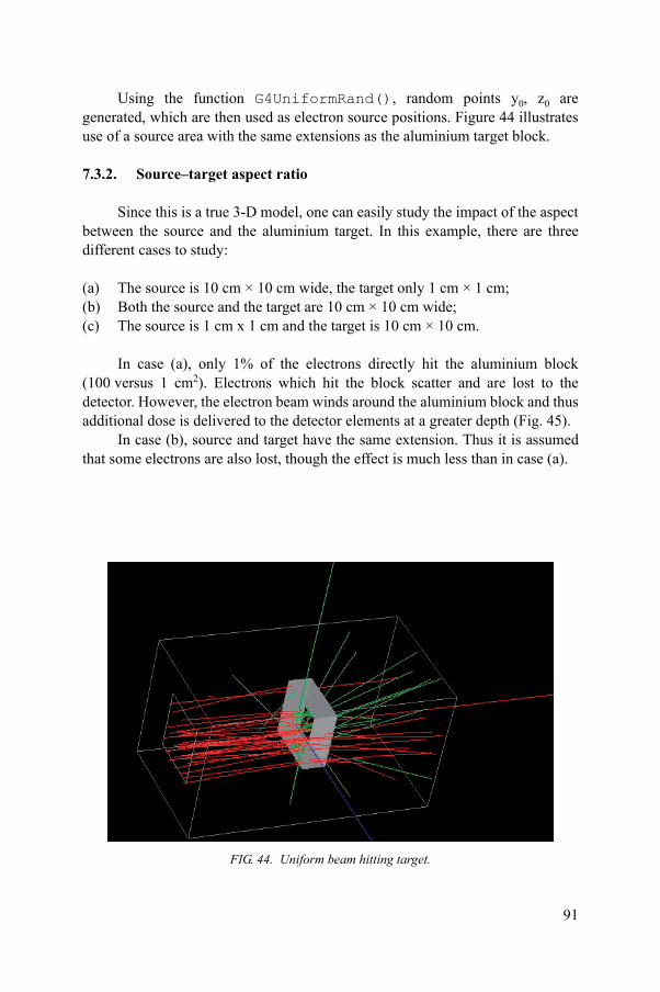
Using the function G4UniformRand(), random points y0, z0 are generated, which are then used as electron source positions. Figure 44 illustrates use of a source area with the same extensions as the aluminium target block.

7.3.2. Source–target aspect ratio

Since this is a true 3-D model, one can easily study the impact of the aspect between the source and the aluminium target. In this example, there are three different cases to study:

(a) The source is 10 cm × 10 cm wide, the target only 1 cm × 1 cm;(b) Both the source and the target are 10 cm × 10 cm wide;(c) The source is 1 cm x 1 cm and the target is 10 cm × 10 cm.

In case (a), only 1% of the electrons directly hit the aluminium block (100 versus 1 cm2). Electrons which hit the block scatter and are lost to the detector. However, the electron beam winds around the aluminium block and thus additional dose is delivered to the detector elements at a greater depth (Fig. 45).

In case (b), source and target have the same extension. Thus it is assumed that some electrons are also lost, though the effect is much less than in case (a).

91

FIG. 44. Uniform beam hitting target.

In case (c), the target has a much wider extension than the source, so it is assumed that almost all electrons deposit their energy into the target cells. This case should be nearly equivalent to the pencil beam topology.

In Fig. 46, all three depth–dose curves are presented in one plot. Please note that cases (a) and (c) are scaled by a factor of 100:1 and 1:100, respectively, to achieve the correct surface dose.

Expectations were achieved: the curves of the pencil beam and the large target nearly overlap. If the source and the target have the same extension, a big difference in the depth–dose curve is already apparent. However, the maximum range of electrons is quite the same. The curve with a large source and a small target is considerably different from the other curves. Dose buildup is hardly noticeable due to escaping electrons. On the other hand, the dose extends to greater depth values, because the beam winds around the detector and delivers dose to regions which cannot be penetrated by direct radiation.

FIG. 45. Small aspect target in uniform beam.

92

From these simple examples, some of the benefits of three dimensional modelling become apparent. Without effort, some interesting effects in radiation physics can be studied which make these models valuable tools in teaching topics related to radiation physics.

7.4. EXAMPLE 3: DOSE BUILDUP

7.4.1. Work plan

In this example, slightly more complex geometry is used to study the effect of dose buildup due to reflection off a boundary.

The basic idea is to design an open box by cutting the interior away from a cube. The bottom of the cube, which is surrounded by high boundary walls, is the detector, where dose distribution is measured. A two dimensional grid with individual detectors of 1 mm × 1 mm is used.

If the interior of the cube is 4 cm × 4 cm, there are 1600 individual detector elements, which should allow for a fine grain analysis of the reflection of walls made of different materials.

Two approaches are used in relation to the beam:

(a) A planar parallel beam (as used in the previous example);(b) A planar scanned beam.

FIG. 46. Comparison of depth–dose curves.

93

Figures 47 and 48 show the geometry of this set-up.

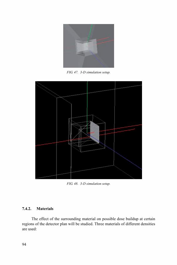
FIG. 47. 3-D simulation setup.

FIG. 48. 3-D simulation setup.

94

7.4.2. Materials

The effect of the surrounding material on possible dose buildup at certain regions of the detector plan will be studied. Three materials of different densities are used:

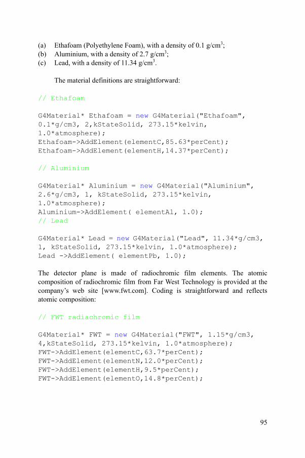
(a) Ethafoam (Polyethylene Foam), with a density of 0.1 g/cm3;(b) Aluminium, with a density of 2.7 g/cm3;(c) Lead, with a density of 11.34 g/cm3.

The material definitions are straightforward:

// Ethafoam

G4Material* Ethafoam = new G4Material("Ethafoam", 0.1*g/cm3, 2,kStateSolid, 273.15*kelvin, 1.0*atmosphere);Ethafoam->AddElement(elementC,85.63*perCent);Ethafoam->AddElement(elementH,14.37*perCent);

// Aluminium

G4Material* Aluminium = new G4Material("Aluminium", 2.6*g/cm3, 1, kStateSolid, 273.15*kelvin, 1.0*atmosphere);Aluminium->AddElement( elementAl, 1.0);// Lead

G4Material* Lead = new G4Material("Lead", 11.34*g/cm3, 1, kStateSolid, 273.15*kelvin, 1.0*atmosphere);Lead ->AddElement( elementPb, 1.0);

The detector plane is made of radiochromic film elements. The atomic composition of radiochromic film from Far West Technology is provided at the company’s web site [www.fwt.com]. Coding is straightforward and reflects atomic composition:

// FWT radiachromic film

G4Material* FWT = new G4Material("FWT", 1.15*g/cm3, 4,kStateSolid, 273.15*kelvin, 1.0*atmosphere);

95

FWT->AddElement(elementC,63.7*perCent);FWT->AddElement(elementN,12.0*perCent);FWT->AddElement(elementH,9.5*perCent);FWT->AddElement(elementO,14.8*perCent);

7.4.3. Geometry

The ‘open cube’ solid in Fig. 48 is made using Boolean operations, which are very powerful in designing complex objects. First an ‘outer’ box is created, which is a 6 cm × 6 cm × 6 cm cube:

G4double Slab_Z = (60.0/2)*mm; // length in conveyor directionG4double Slab_Y = (60.0/2)*mm; // length in scan directionG4double Slab_X = (60.0/2)*mm; // length in beam direction

G4Box* Slab = new G4Box("Slab",Slab_X,Slab_Y,Slab_Z);

Note that the parameter definition above may look strange, but actually minimizes errors when coding geometries. Solids in GEANT4 are usually parametrized from the perspective of the centre of the object. So the parameters x, y, z in the definitions refer to the half length, width and height. This may cause confusion and errors during the coding of geometries. It is thus wise to use the notation provided in the example, in which one divides the full extension by two. Since the geometry setting is only executed once, there is no run time overhead. GEANT4 explicitly uses units, so it is wise to add the unit to any variable definition.

The cube cavity is made up of another solid, which we then subtract from the cube using a Boolean operation:

/// The inner block which defines the interior of the cube

G4double Box_Inner_x = (60.0/2)*mm; // in beam directionG4double Box_Inner_y = (40.0/2)*mm; // in scan directionG4double Box_Inner_z = (40.0/2)*mm; // in conveyor

96

directionG4Box* Box_Inner = new G4Box("Box_Inner",Box_Inner_x,Box_Inner_y,Box_Inner_z);

The block is given the same dimension in beam direction, but 20 mm less in conveyor and scan directions. Therefore the walls of the object are 10 mm thick.

The Boolean operation, which subtracts the inner box from the outer cube, is made with one line of code. Normally the two solids share the same origin regarding the coordinate system. Since it is desirable to have a 10 cm thick cube bottom, a simple shift of 10 mm is made to the inner box using the G4ThreeVector(shift_x,0.,0.) command:

G4double shift_x = -10*mm;G4SubtractionSolid* bO_minus_bI = new G4SubtractionSolid ("Hull", Slab,Box_Inner,0,G4ThreeVector(shift_x,0.,0.)); // shift

The detector plane is placed at the bottom of the cavity. There are several methods to place grids. The simplest is the repeated placement of an individual 1 mm × 1 mm detector element. Coding is done using two nested loops, as shown in the following code fragment:

// detector element

G4double Box01_z= 0.5*mm;G4double Box01_y= 0.5*mm;G4double Box01_x= 0.5*mm;

// make simpler Variable names

G4double dXH = Box01_x;

G4double dY = 2.*Box01_y;G4double dYH = Box01_y;G4double y1 = -20*mm;G4double y2 = 20*mm;

G4double dZ = 2.*Box01_z;G4double dZH = Box01_z;

97

G4double z1 = -20*mm;G4double z2 = 20*mm;

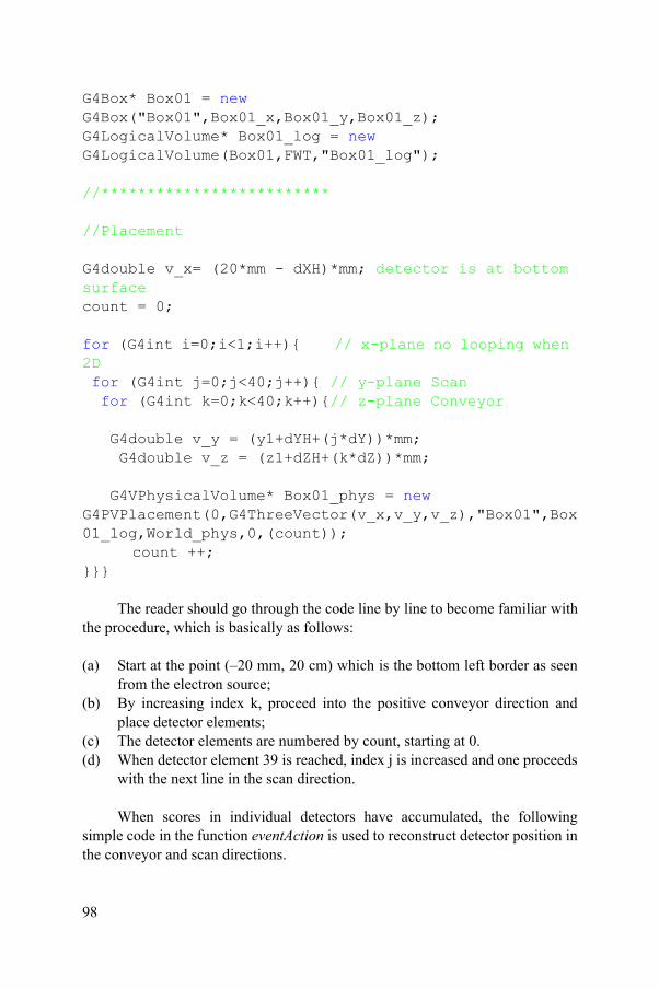
G4Box* Box01 = new G4Box("Box01",Box01_x,Box01_y,Box01_z);G4LogicalVolume* Box01_log = new G4LogicalVolume(Box01,FWT,"Box01_log");

//*************************

//Placement

G4double v_x= (20*mm - dXH)*mm; detector is at bottom surfacecount = 0;

for (G4int i=0;i<1;i++){ // x-plane no looping when 2D for (G4int j=0;j<40;j++){ // y-plane Scan for (G4int k=0;k<40;k++){// z-plane Conveyor G4double v_y = (y1+dYH+(j*dY))*mm; G4double v_z = (z1+dZH+(k*dZ))*mm;

G4VPhysicalVolume* Box01_phys = new G4PVPlacement(0,G4ThreeVector(v_x,v_y,v_z),"Box01",Box01_log,World_phys,0,(count));

count ++;}}}

The reader should go through the code line by line to become familiar with the procedure, which is basically as follows:

(a) Start at the point (–20 mm, 20 cm) which is the bottom left border as seen from the electron source;

(b) By increasing index k, proceed into the positive conveyor direction and place detector elements;

(c) The detector elements are numbered by count, starting at 0.

98

(d) When detector element 39 is reached, index j is increased and one proceeds with the next line in the scan direction.

When scores in individual detectors have accumulated, the following simple code in the function eventAction is used to reconstruct detector position in the conveyor and scan directions.

X = 0;G4int help =detectorNumber[k];Y = help / 40; // row of the detector array (scan direction)Z = help % 40; // column of the detector array (conveyor direction)

Detector grid layout with associated detector numbers is explained in Fig. 49.

7.4.4. Results for planar beam

The plots in Figs 50, 51 and 52 show dose distribution for ethafoam, aluminium and lead.

99

FIG. 49. Detector grid layout.

FIG. 50. Planar beam ethafoam.

100

FIG. 51. Planar beam aluminium.

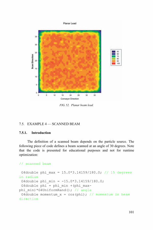
7.5. EXAMPLE 4 — SCANNED BEAM

7.5.1. Introduction

The definition of a scanned beam depends on the particle source. The following piece of code defines a beam scanned at an angle of 30 degrees. Note that the code is presented for educational purposes and not for runtime optimization: // scanned beam

G4double phi_max = 15.0*3.14159/180.0; // 15 degrees

FIG. 52. Planar beam lead.

101

in radian G4double phi_min = -15.0*3.14159/180.0; G4double phi = phi_min +(phi_max-phi_min)*G4UniformRand(); // angle G4double momentum_x = cos(phi); // momentum in beam direction

G4double momentum_y = sin(phi); // component in scan direction G4double z0_min = -10.0*cm; // mins and maxs in conveyor direction G4double z0_max = 10.0*cm;

G4double x0 = -14*cm; // place gun in x G4double y0 = 0.0*cm; // symmetric scan around zero G4double z0 = z0_min+(z0_max- z0_min)*G4UniformRand(); //spread in z

particleGun->SetParticlePosition(G4ThreeVector(x0,y0,z0)); particleGun->SetParticleMomentumDirection (G4ThreeVector(momentum_x,momentum_y,0.0)); particleGun->GeneratePrimaryVertex(anEvent);

The plot in Fig. 53 shows 20 electron trajectories of the scanned beam.

102

FIG. 53. Twenty electron trajectories of a scanned beam.

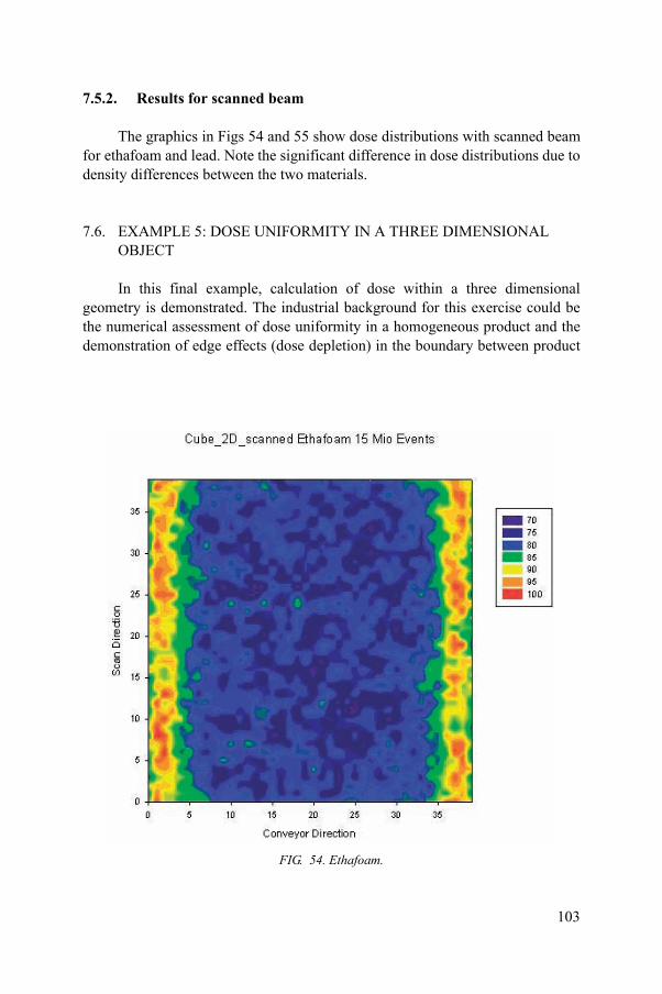
7.5.2. Results for scanned beam

The graphics in Figs 54 and 55 show dose distributions with scanned beam for ethafoam and lead. Note the significant difference in dose distributions due to density differences between the two materials.

7.6. EXAMPLE 5: DOSE UNIFORMITY IN A THREE DIMENSIONAL OBJECT

In this final example, calculation of dose within a three dimensional geometry is demonstrated. The industrial background for this exercise could be the numerical assessment of dose uniformity in a homogeneous product and the demonstration of edge effects (dose depletion) in the boundary between product

103

FIG. 54. Ethafoam.

and air. For simplicity we use choose a box, which allows us to reuse previous geometry coding.

7.6.1. Geometry input

A 3-D object constructed as a cube is built of 20 × 20 × 20 = 8000 detector elements, each with a dimension of 1 mm × 1 mm × 1 mm. This fine granularity allows us to view dose distribution in a 2 cm × 2 cm × 2 cm cube in detail.

The idea is to put the object in the centre of the coordinate system and assemble the cube by positioning individual detectors Box01 along the beam, scan, and conveyor axis.

FIG. 55. Lead.

104

To facilitate programming, some variables are defined which make the problem more transparent.

G4double dXH = Box01_x; // half extension in x (beam direction)G4double dX = 2.*Box01_x; // extension in x (beam direction)G4double dY = 2.*Box01_y; // same in y (scan)G4double dYH = Box01_y;G4double dZ = 2.*Box01_z; // same in z (conveyor)G4double dZH = Box01_z;

G4double x1 = -10.0*mm; //start - end beam directionG4double x2 = 10.0*mm;

G4double y1 = -10.0*mm; // start - end scan directionG4double y2 = 10.0*mm;

G4double z1 = -10*mm; // start - end conveyorG4double z2 = 10*mm;

The detector element is defined as 1 × 1 × 1 mm aluminium cubes:

G4double Box01_z= 0.5*mm;G4double Box01_y= 0.5*mm;G4double Box01_x= 0.5*mm;

G4Box* Box01 = new G4Box("Box01",Box01_x,Box01_y,Box01_z);G4LogicalVolume* Box01_log = new G4LogicalVolume(Box01,Aluminium,"Box01_log");

The 3-D box is constructed simply through the following loops, in which individual detectors are placed in their proper position. The predefined variables create an easy to read coding:

count = 0;

105

for (G4int i=0;i<20;i++){ // x-plane for (G4int j=0;j<20;j++){ // y-plane Scan for (G4int k=0;k<20;k++){ // z-plane Conveyor

G4double v_x = (x1+dXH+(i*dX))*mm; G4double v_y = (y1+dYH+(j*dY))*mm; G4double v_z = (z1+dZH+(k*dZ))*mm;

G4VPhysicalVolume* Box01_phys = new G4PVPlacement(0,G4ThreeVector(v_x,v_y,v_z),"Box01",Box01_log,World_phys,0,(count));

count ++;}}}

The variable ‘count’ describes the detector number, starting from 0 and going up to 7999. This simple scheme of multiple detector placements allows for even more detectors and has the benefit of easy dose calculation and result visualization. Figure 56 displays the detector layout used in this example.

7.6.2. Dose calculation

The principal action of calculating dose in each detector cell is made to output the detector array (0 to 7999) to form an X (beam), Y (scan) and Z (conveyor) spreadsheet. This is done as follows:

106

FIG. 56. Detector layout.

std::ofstream OutEnergyFile; OutEnergyFile.open("logfile_detector.txt"); OutEnergyFile.precision(10);

for (G4int k=0;k<NbDetectorEntries;k++) {

G4int X,Y,Z; // X = Beamdirection Y = Scan Direction // Z = Conveyor Direction

X= detectorNumber[k]/ 400; // product of Y und Z number of bins

G4int help= detectorNumber[k] % 400; Y = help / 20; Z = help % 20;

OutEnergyFile << detectorArray[k] << ";" << detectorNumber[k] << ";" << X << ";" << Y << ";" << Z << " }

The code above is easy to follow when consideration is made for how the box was constructed: the X coordinate is the layer of 20 × 20 = 400 detectors in the beam direction, starting from the box surface facing the beam. Therefore, the x coordinate is provided by dividing the detector number (starting with 0) of the detector grid by 400. Note that the absolute position would be –10 mm plus the detector x coordinate. In the same manner, y and z coordinates are calculated, leaving three numbers which describe a particular grid cell.

This triplet and associate stored energy in eV are kept in the log file logfile_detector.txt, which can then be read and analysed using an external program.

7.6.3. Analysis

The analysis of a detector grid with 8000 cells is best done using a dedicated program specialized in voxel visualization. Each detector or voxel is

107

described in space using (x, y, z) coordinates; the stored energy (proportional to dose) is the associated value to be visualized.

There are many non-commercial and high end commercial programs specializing in volume visualization and it is beyond the scope of this work to provide an extensive survey5.

Figures 57, 58 and 59 contain pictures of an ethafoam block irradiated by 10 MeV electrons. Note that the detector (0,0,0) describes the left bottom corner of the box, whereas the upper right corner is (19,19,19).

Volume visualization delivers a fine grain picture of dose distribution in the box. A planar, parallel beam is used and thus edge effects can be clearly seen: electrons interacting at the edges of the product are scattered out towards the air. From the outside fewer electrons enter the edges, so a lack of electron equilibrium is manifested by dose depletion at the corners.

A numerical analysis provides a Dmax/Dmin ratio of 2.1, which is striking for such simple geometry. The effect disappears with use of a scanned beam.

108

5 The program VOXLER from Golden Software was used for this work (www.goldensoftware.com).

FIG. 57. Ethafoam block irradiated by 10 MeV electrons.

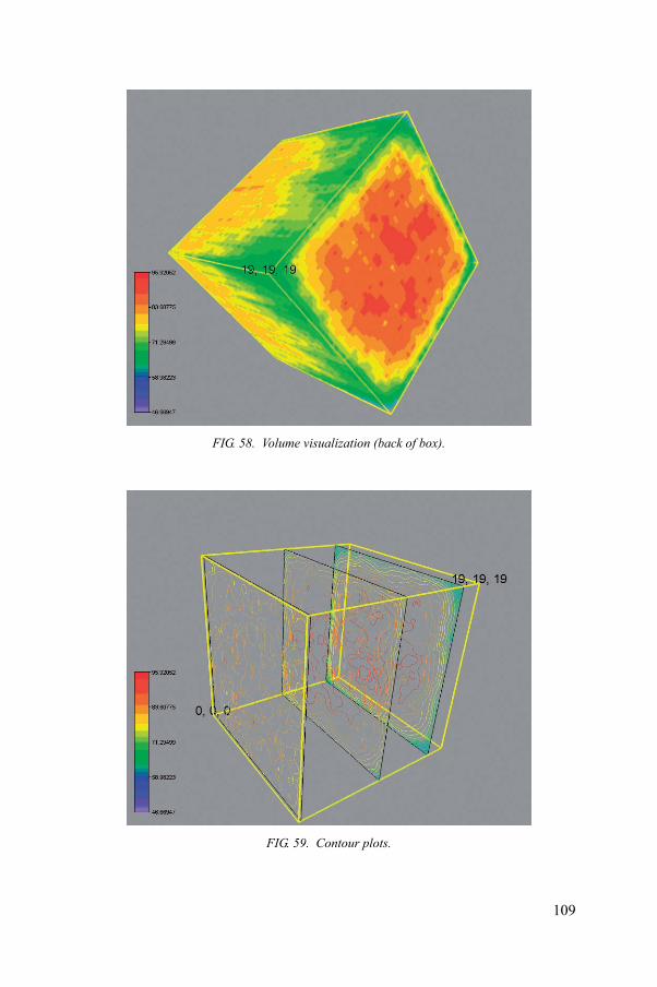
FIG. 58. Volume visualization (back of box).

109

FIG. 59. Contour plots.

Another tutorial picture is provided, in which ethafoam is replaced by aluminium. One clearly sees an edge effect in the 2 × 2 × 2 cm aluminium block (Fig. 60).

7.7. CONCLUSION

Three dimensional modelling is definitely the most demanding, but also the most valuable tool which can be used to describe and visualize the interaction of radiation with matter. Even simple geometries requiring only minimum effort for description provide interesting insight into achieved dose distributions and can serve to explain effects and phenomena in radiation physics.

To model more complex geometries, much more effort is required to

FIG. 60. 2 × 2 × 2 cm aluminium block.

110

describe geometry and dose analysis in an area of interest. The time and cost required to code industrial geometries certainly limits every day use, for example, as a tool to support dose mapping.

Methods borrowed from medical physics and radiation therapy are currently finding their way into industrial applications. The required steps are:

(1) Import geometry from CAD files;(2) Generate a conformal mesh;(3) Calculate dose distribution using radiation transport codes.

This mesh methodology, together with refined geometry modelling and faster computers, provides a promising outlook for the future of modelling in industrial irradiation. One dimensional analysis is quick and efficient, but the future certainly belongs to 3-D modelling.

111

.

REFERENCES

[1] INTERNATIONAL ORGANIZATION FOR STANDARDIZATION, ISO/ASTM 51649:2002 Standard Practice for Dosimetry in an Electron Beam Facility for Radiation Processing at Energies Between 300 keV and 25 MeV, ISO, Geneva (2002).

[2] INTERNATIONAL ORGANIZATION FOR STANDARDIZATION, ISO/FDIS 11137, Sterilization of Health Care Products — Radiation — Part 1: Requirements for Development, Validation and Routine Control of a Sterilization Process for Medical Devices, ISO, Geneva (2006).

[3] INTERNATIONAL ORGANIZATION FOR STANDARDIZATION, ISO/ASTM 51649:2005, Practice for Dosimetry in an Electron Beam Facility for Radiation Processing at Energies between 300 keV and 25 MeV, ISO, Geneva (2005).

[4] AMERICAN SOCIETY FOR TESTING AND MATERIALS, ASTM E 2232, Standard Guide for Selection and Use of Mathematical Methods for Calculating Absorbed Dose in Radiation Processing Applications, ASTM, Conshohocken.

[5] EUROPEAN ORGANIZATION FOR NUCLEAR RESEARCH, GEANT4 Physics Reference Manual, GEANT4 Collaboration, www.cern.ch/geant4

[6] SALVAT, F., “Overview of Monte Carlo”, Int. Workshop on Monte Carlo Codes, Teddington, National Physical Laboratory (2007).

[7] BERGER, M.J., “Monte Carlo calculations of the penetration and diffusion of fast charged particles”, Methods in Computational Physics, Vol. 1 (ALDER, B., et al.), Academic Press (1963) 135–215.

[8] BIELAJEW, A. F., Fundamentals of the Monte Carlo Method for Neutral and Charged Particle Transport, University of Michigan, Department of Nuclear Engineering and Radiological Sciences, http://www-personal.umich.edu/~bielajew/MCBook/book.pdf

[9] BIELAJEW, A.F., ibid.[10] MATLAB, The MathWorks Inc. (2008), www.mathworks.com[11] http://www.randomnumbers.info/content/About.htm[12] BIELAJEW, A. F., Fundamentals of the Monte Carlo Method for Neutral and Charged

Particle Transport, The University of Michigan, Department of Nuclear Engineering and Radiological Sciences, http://www-personal.umich.edu/~bielajew/MCBook/book.pdf

[13] BIELAJEW, A.F., ibid.[14] THE IRRADIATION PANEL, Review of Monte Carlo Modelling Codes, London

(2007), http://www.irradiationpanel.org/publications/publications.asp[15] TAGZIRIA, H., Review of Monte Carlo and Deterministic Codes in Radiation

Protection and Dosimetry, National Physical Laboratory, Teddington (2000).[16] INTERNATIONAL ORGANIZATION FOR STANDARDIZATION, ISO 11137:2006.[17] THE IRRADIATION PANEL, Review of Monte Carlo Modelling Codes, London

(2007), http://www.irradiationpanel.org/publications/publications.asp[18] SALVAT, F., FERNANDEZ-VAREA, J.M., SEMPAU, J., “PENELOPE — A code

113

system for Monte Carlo simulation of electron and photon transport”, Proc. Workshop, Issy-les-Moulineaux (2003).

[19] AGOSTINELLI, S., et al., “G4 — a simulation toolkit”, Nuclear Instruments and Methods in Physics Research Section A: Accelerators, Spectrometers, Detectors and Associated Equipment, 506 3 (2003) 250–303.

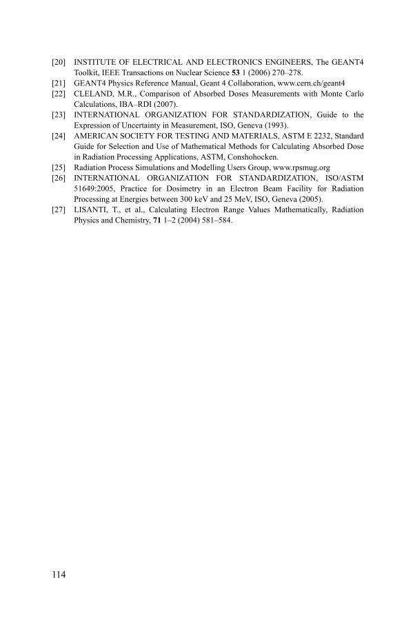
[20] INSTITUTE OF ELECTRICAL AND ELECTRONICS ENGINEERS, The GEANT4 Toolkit, IEEE Transactions on Nuclear Science 53 1 (2006) 270–278.

[21] GEANT4 Physics Reference Manual, Geant 4 Collaboration, www.cern.ch/geant4[22] CLELAND, M.R., Comparison of Absorbed Doses Measurements with Monte Carlo

Calculations, IBA–RDI (2007).[23] INTERNATIONAL ORGANIZATION FOR STANDARDIZATION, Guide to the

Expression of Uncertainty in Measurement, ISO, Geneva (1993).[24] AMERICAN SOCIETY FOR TESTING AND MATERIALS, ASTM E 2232, Standard

Guide for Selection and Use of Mathematical Methods for Calculating Absorbed Dose in Radiation Processing Applications, ASTM, Conshohocken.

[25] Radiation Process Simulations and Modelling Users Group, www.rpsmug.org[26] INTERNATIONAL ORGANIZATION FOR STANDARDIZATION, ISO/ASTM

51649:2005, Practice for Dosimetry in an Electron Beam Facility for Radiation Processing at Energies between 300 keV and 25 MeV, ISO, Geneva (2005).

[27] LISANTI, T., et al., Calculating Electron Range Values Mathematically, Radiation Physics and Chemistry, 71 1–2 (2004) 581–584.

114

CONTRIBUTORS TO DRAFTING AND REVIEW

Haji-Saeid, M. International Atomic Energy Agency

Lazurik, V. Radiation Physics Laboratory, Kharkov National University, Ukraine

Mitterndorfer, J. High Tech Consulting and Technical Advisor to Mediscan GmbH, Austria

Sampa, M.H.O. International Atomic Energy Agency

Zimek, Z. Institute of Nuclear Chemistry and Technology, Poland

115

@������

��������� ���������������� ��������������������������������� �������������������������� ������������ ���������

����������������������������������� �������������������������������� ����� !"����������

������ �#��������� ��� ��$�����%&'�(� �������)�����*�+!,�*�-.-/��

+�������0�1%.�-�2/.3�4444�5�6�70�1%.�-�2/.3�44''��

���0����$��8������ ��������5�(���� �0�� �099���������� ��������

!� " �#:�������;��������$��������)��/3/��<=..23�<��������

+�������0�1-/�/�>-'�&-�3'�5�6�70�1-/�/�>-'�3'�&.��

���0��������������8������������5�(���� �0�� �099��������=��=���������

$���%�<������������ ����&>3.�6������<$��� � ��/33��;�������*#�/343%=&-&%��� ���

+�������0�.='33='%>=-&>4�5�6�70�.='33='%>=-&>3��

���0���� ��������8�����������5�(���� �0�� �099���������������

)������������?�!�������; ����.=>-%2�!��� ���)����" �����"� �����@.:�2:-��

+�������0�1%.-�4&>�/%%>�5�6�70�1%.-�4&>�4%%3��

���0���������� 8����������������5�(���� �0�� �099��������������������

$& ������������ ������!�����0�!���������������?������� ���!������ ����+����� ��� �� ������"��<�7�/.3-��<���?�

$'�$&���(�! $ ������!A�� �)�"���@�����$��-&4��.'3�/.�������2��

+�������0�1&/3�/%%3-�>-%&�5�6�70�1&/3�/'&'/�.%&%��

���0������8��������B�5�(���� �0�� �099������������B�

) � ��%��� �������@������������"�<"C�./'�D@������� ��.E��6��=33.3.�,������

+�������0�1->'�2�./.�&.�5�6�70�1->'�2�./.�&&>3��

���0���� ���8��� �����������5�(���� �0�� �099������� �����������

)���$�6���=�� ��>������:����������"��<�7�/>��6=4>2/.������!���7�.2��

+�������0�1--�.�&/�3.�&2�&2�5�6�70�1--�.�&/�3.�23�23��

���0������� 8������ ����5�(���� �0�� �099����������� ����

;�$����� � ��.&>�����������$?����2&/-%�!������!���7��

+�������0�1�--�.�&4�&3�%4�3/�5�6�7�1--�.�&4�&3�%4�3/��

���0��������$�����8�$��������5�(���� �0�� �099�����$��������

"��#��*��"=F���?��F�� ����=�����F���?��G��,�����,��?�� ���.3��#=>-..-�<�����

+�������0�1�&2�//'�2&�23�/3�5�6�70�1&2�//'�2&�23�/3����1&2�//'�2&�23�///��

���0���� ���?8���=$���?����5�(���� �0�� �099�������=$���?����

&��"��*;��� �����; ����<��������� ����"��<�7�./%��,=.%>%�<������ ��

+�������0�1-%�.�/>4�4444�5�6�70�1-%�.�/>4�4&4/�5����0������8��� ��������

�% ��������������G������.� �6�����#������,������.>��:�����,������*��?��<������� � ���*�����&33�33.���

+�������0�12.�//�//%.42/%9/4�5�6�70�12.�//�//%.42/'��

���0�����8$�������5�(���� �0�� �099��������������������

<�������/94/����������!������#���..3332��

+�������0�12.�..�/-/%'4'%��12.�..�/-/>4/%&�5�6�70�12.�..�/-/'.-.>��

���0�������8$����� �

�� *;������ ��� H���#� ��;������<����I���"�J��F��!������%���=/3.&%�*����

+�������0�1-2�3/�&'�2>�&>�>/����&'�2>�&>�%/�5�6�70�1-2�3/�&'�2>�&>�&'��

���0����8�������������5�(��� �0�����������������

+�(��*���B���!��������; ����.-=%�����������-��������!���=����+�����.3-=33/4��

+�������0�1'.�-�-/4>�'>'/�5�6�70�1'.�-�-/4>�234/��

���0�������8����B���������5�(���� �0�� �099��������B���������

��(�! $�,)�-,���@�� �������������� ���<�������#�� �� �����<�?��/���6�����/4>=.�K��?�:��=���?� ��!��=G�� ����.-4=.-3�

+�������0�13/�>'2�.4&3�5�6�70�13/�>'2�.4&%�5�(���� �0�� �099��������������

���&�� ��%�#��;���������� ���� ���������� ���<�F���*�������)�� ��� ��� �/3����;=4&'/�<A�,�������?����

+�������0�1-.�D3E�>-�>4&333&�5�6�70�1-.�D3E�>-�>4/2/2%��

���0������8��������������5�(���� �0�� �099������������������

*�� ������������� ���� �����@���������>3����"��<�7�.'>-��/433�!A�A�� ��������

+�������0�1-.�42-�%'&�&33�5�6�70�1-.�42-�%.>�%2'��

���0����8���������5�(���� �0�� �099�������������

�� ������A� �?�����$�����"��<�7�'-3��/.%3� A�;�����

+�������0�1-.�/>/�&->�...�5�6�70�1-.�/>/�&.>�'''��

���0������8��� ����5�(���� �0�� �099������� ����

����'�� ��%#��������� ��� ��$�����%&'�(� �������)�����*�+!,�*�-.-/����� �����

+�������0�1%.�-�2/.3�4444�5�6�70�1%.�-�2/.3�44''��

���0����$��8������ ��������5�(���� �0�� �099���������� ��������

� ,.�� �!�������$��A��B���������@�� ����$��/�� �=.>./�;���������

+�������0�1-'%�.�&-/�-.�&&�5�6�70�1-'%�.�/-3�.&�->��

���0����� ������8��������$�=B���5�(���� �0�� �099������������$�=B��9�$�B�

�(� �#L�B���� �� ���� ������9�:����<��$���-����=/'33%�*������

+�������0�1-&�2.�4'.�2&�'3�5�6�70�1-&�2.�>4>�>>�%-��

���0��������8��B����� �������������8��B����� ���������������8��B����� ����������8��B����� �����

(���� �0�� �099������B����� ������

�� ��%�- �"%,#+��� � ������"�H���; ����� ���� ���� �����?�������"�<�7�/2�����������)-�.�G���

+��������D������E0�1&&�'43�%33�>>>/�5�D��M����E0�1&&�/34�'4-�'-4/�5�6�70�1&&�/34�'4-�'/3-��

����D������E0������������8 ���������5�D��M����E0��������M����8 ���������5�(���� �0�� �099���� ���������

"�=�����������

#�;+���� ��<����(���������; ����-2���7������)���������� ����� �������@+.>�/�N��

���0����8��������������5�(���� �0�� �099������������������

<�������� �����$������ ��

��� ���� �; ������"��<�7�..2�� �$���?�� G.�&+���

+�������0�1&&�.&-'4&'...�5�6�70�1&&�.&-'4&''&&��

���0�������8��� ���� �����5�(���� �0�� �099������� ���� ����

�� ��%���� ,��#�� ���33&��)����#!/=3'>-��6�� ��$������ �&% �� ��� ������K�������K��.33.4��� ���

D��E�+�������0�1'33�/>-=2%&%����1/./�2%-='-3/�5�6�70�1/./�2%-=-&'2��

���0������ ���8�����?�5�(���� �0�� �099���������?�

�� ��%��������,)��#�� $�<������������ ����&>3.�6������<$���� � ��/33��;�������*#�/343%=&-&%�

+�������0�.='33='%>=-&>4�5�6�70�.='33='%>=-&>3��

���0���� ��������8�����������O�(���� �0�� �099���������������

)������������?�!�������; ����'./����� ����$����"?�������?���K��.-%%2��

+�������0�1'''�>>.�4&43�D �=����E�5�6�70�1'''�>%'�'>&%�D �=����E��

���0���������� 8����������������5�(���� �0�� �099��������������������

,�������/������������0������������������������������� �� �0�

#�1������������������2� ��������������0������3�����3��

F������� ���� ����!�� �����"�<�7�.33��.&33�F��������� ���

+�������0�1&-�.�/%33�//>/2�D���//>-3E�5�6�70�1&-�.�/%33�/2-3/�

���0����������� ���8������?�5�(���� �0�� �099����������?9�����

10-3

8771

This publication is intended to serve as both a guidebook and introductory tutorial for the use of mathematical modelling (using mostly Monte Carlo methods) in electron beam processing. The emphasis of this guide is on industrial irradiation methodologies, with extensive reference to existing literature and applicable standards. Its target audience is readers who have a basic understanding of electron beam technology and want to evaluate and apply mathematical modelling for the design and operation of irradiators, and those who wish to have a better understanding of irradiation methodology and process development for new products.

INTERNATIONAL ATOMIC ENERGY AGENCYVIENNA

ISBN 978–92–0–112010–6ISSN 2220–7341

IAEA RAD

IATION

TECH

NO

LOGY SER

IES No. 1

IAEA RADIATION TECHNOLOGY SERIES No. 1

Use of Mathematical Modelling in Electron Beam Processing: A Guidebook

10-38771_P1474_cover.indd 1 2011-01-14 14:43:06