Use of Geochemistry Data Collected by the Mars Exploration RoverSpirit in Gusev Crater to Teach Geomorphic Zonation throughPrincipal Components AnalysisChristine M. Rodrigue1,a)

ABSTRACTThis paper presents a laboratory exercise used to teach principal components analysis (PCA) as a means of surface zona-tion. The lab was built around abundance data for 16 oxides and elements collected by the Mars Exploration Rover Spiritin Gusev Crater between Sol 14 and Sol 470. Students used PCA to reduce 15 of these into 3 components, which, afterquartimax rotation, very strikingly divided the surface traversed by Spirit’s into three distinct zones. Students then usedsuch concepts as the Bowen reaction series, typical minerals in Earth’s basalts and andesitic arcs, the periodic table, andthe Goldschmidt classification, together with Pancam images from Spirit and the Mars Orbiter Camera, to interpret thesurfaces over which the rover moved. Students found this foray to Mars a challenging but enjoyable project, and it madePCA memorable to them long after the class had ended. Some variant on this lab could work for multivariate statisticscourses in geology, geography, and environmental science, as well as advanced courses in the content of those disciplines,particularly those dealing with zonation. VC 2011 National Association of Geoscience Teachers. [DOI: 10.5408/1.3604826]

INTRODUCTIONThis paper presents an exercise that uses Mars Explora-

tion Rover geochemical data to teach principal componentsanalysis (PCA) for geomorphic or geological zonation. Thedata come from the Spirit rover’s Alpha Particle X-ray Spec-trometer (APXS), which collected spectra from 93 rocks andsoil samples (Gellert et al., 2006) during its travel over threedistinctive zones on the floor of Gusev Crater. These zonesconsisted of a cratered basaltic plain, the West Spur of theColumbia Hills with bedded materials and evaporites, andthe northwest side of Husband Hill where very diverseaqueous and acid–aqueous altered rocks and soils werefound. PCA is a data reduction technique that has increas-ingly been used in the geosciences since the early 1960s,making its acquaintance of value in the education of geosci-ence majors. The APXS data can make the technique memo-rable to such majors as it produces a coherent zonationfrom 15 different oxides and elements.

A classic task in the geosciences is zonation of complexsurface patterns into areal units and demarcating transitionzones or boundaries between them, often along a transectin the field. So, for example, a soil catena can be zoned bychanges in soil particle size, underlying bedrock and rego-lith, topographic relief, drainage, erosion and depositionprocesses, weathering, organic matter, and geochemistry(Milne 1935; Bushnell, 1942; Webster, 1973; Raynolds et al.,2006). Ground-penetrating radar can be used along a tran-sect to infer subsurface stratigraphy for geological map-ping (Baker and Jol, 2007). An environmental ecotonemight be zoned by field sampling of soils and censusing ofspecies presence and abundance along a transect. For

example, a transect could be taken down a catena, across awetland–upland interface, or through a seasonal surfacewater and groundwater boundary (Fortin et al., 2000).

Zonation can be vertical and temporal in geologicalusage, not just horizontal and spatial in mapping usage.So, for example, fossils, grain size, bulk density, and geo-chemistry can be used for temporal zonation and sequenc-ing of stratigraphic units (e.g., Patterson et al., 2000; Brownand Pasternack, 2004; Peterson et al., 2008).

Zonation, then, is a common task in the field and labo-ratory activities of geoscientists. The process can seemsuperficially straightforward, but the zoning schemes thatresult can color analytic results. Complications includescale, edge effects, spatial autocorrelation, and aggregationeffects. These distortions and biases are collectively calledthe Modifiable Areal Unit Problem or MAUP (Dark andBram, 2007) or the analogous Modifiable Temporal UnitProblem (MTUP). The MTUP is less commonly discussed,largely in criminology contexts (e.g., Taylor, 2010), but it isclearly relevant to geoscientists’ work. Concern about zon-ing has driven development of statistical techniques to letimage processing, GIS, and statistical software handle thekinds of remote sensing, field, and laboratory data gener-ated and used by geoscientists.

One of the common statistical techniques used in zona-tion is principal components analysis or PCA, a member ofthe factor analytic (FA) family of techniques. PCA is pri-marily concerned with data reduction or grouping of manyvariables into fewer components. FA is mainly concernedwith identifying or testing underlying factors that may notbe directly measurable themselves but which are expressedin commonalities in measurements of empirical variables(Bryant and Yarnold, 1995; Rogerson, 2006; Davis, 2002).PCA is more empirical and inductive; FA is more theoreti-cal and in some versions can test deductive hypothesesabout expected underlying factor structure.

In the geosciences, PCA/FA is a common methodunderlying the unsupervised classification of remote

Received 10 January 2010; revised 2 April 2011; accepted 13 April 2011; pub-lished online 14 November 2011.

a)Electronic mail: rodrigue@csulb.edu

1Department of Environmental Science and Policy and Department ofEmergency Services Management, California State University, LongBeach, California 90840-1101, USA

1089-9995/2011/59(4)/184/10/$23.00 VC Nat. Assoc. Geosci. Teachers184

JOURNAL OF GEOSCIENCE EDUCATION 59, 184–193 (2011)

sensing imagery. It can also be performed on large data setscollected in the field. These could include sampling downthrough a geological column, sediment core, or ice core, forexample, or to process observations across space, as is thecase in the laboratory exercise presented here. It can, thus,assist in both temporal and spatial zonation, making it atool of increasing utility to a variety of geoscientists. Forthat reason, PCA/FA, particularly PCA, is increasinglyencountered in the geoscience literature since its discipli-nary debut in the early 1960s (e.g., Reyment, 1961; Wong,1963; Imbrie and Van Andel, 1964). For that reason, practicein its application would enhance the professional prepara-tion of geoscience students, especially at the advancedundergraduate and beginning graduate levels.

For all its usefulness, PCA/FA is not the most “userfriendly” approach for students. The mathematical com-plexities are now easily handled by the common statisticalsoftware packages. These include SPSS, STATISTICA, MINITAB,MATLAB, SCILAB, R, the freeware programs PAST and WINI-DAMS, and others, Their widespread availability makesPCA/FA accessible to undergraduate students. The under-lying concepts, however, are difficult to convey, becausePCA/FA represents the many variables in the analysis asdimensions and the data collected as occupying an n-dimensional data cloud. Trying to “visualize” this is a toughsell to students! The point of PCA, especially, is to reducethe dimensionality of the data cloud to a small number ofusually orthogonal components. These can then be pro-jected through the data cloud and aligned with most of thedata points when “viewed” through various “rotations” ofthe emergent model. Each of the original variables will“load” highly along one of the components (some may loadless dramatically on more than one component). That is,most of the original variables will show strong correlationswith one of the artificial variables, or components. Theresult for geoscientists can be a meaningful zonation of timeor space. PCA zonation is generated from the data them-selves, rather than from a priori schemes that can give riseto the MAUP and MTUP. The only way to motivate stu-dents to acquire this tool is to show it in operation on a dataset that otherwise would overwhelm them but, processed inPCA, becomes intelligible to them.

Anyone who has ever taught a statistics course knowsthat the worst part is finding or creating a data set thatmeets the requirements of a given technique, producesresults that can enable teachable moments, and, ideally,has something to do with the discipline in which the statis-tics course is taught. This paper introduces a geoscience-related data set, discusses how it was shaped for classroomuse, shows the results of a PCA taught through its use, andthen evaluates student outcomes. The exercise vividlymodels the utility of PCA for geochemical data reductionand geomorphic zonation.

The database contains 16 oxide and element abundan-ces collected from untouched, brushed, or abraded rocks,which were selected by the Mars Exploration Rover scienceteam for APXS during Spirit’s traverse in Gusev Crater. Thelab exercise, using SPSS and Excel, is available at <http://www.csulb.edu/�rodrigue/geog400/project5.html>.

DATA AND METHODSThe data were originally published in Gellert et al.,

2006, where they are presented in the second table of the

article. This table can be saved as a tab-delimited file forimport into a spreadsheet program. There, the data can befurther edited to fit the needs of a statistical software pro-gram or an instructor’s goals.

This table has as the record labels the “sol” or the mar-tian day after landing, on which the sample record wastaken. The table covers the first 470 sols of Spirit’s activ-ities. Martian sols are slightly longer than Earth days at 24h, 37 min, and 23 s, and the date of landing for Spirit was 4January 2004 on Earth. The second variable is the type ofsurface from which Spirit’s APXS took spectra on a givensol. These include rock undisturbed by Spirit (RU), rockbrushed off (RB), rock “RATted” or abraded by the rockabrasion tool (RAT), RAT fines or abrasion debris (RF), soilundisturbed (SU), soil disturbed (SD), and soil trenched(ST). The third variable is the sometimes whimsical nick-name given to an individual rock or soil surface. Norm orgeometric norm is a relative measure of the standoff dis-tance between the APXS and the sample surface in milli-meters. This distance affects how much backgroundelemental noise is included in a reading. The variable nor-malizes the sum of all oxides to 100% to allow measure-ment of relative contributions by each oxide or element. Tis the time in hours that the instrument took to integratethe spectrum. Following these three columns are two col-umns for each of the oxides and elements. The first givesthe relative abundances of the 12 oxides (wt. %) and 4 ele-ments (parts per million), and the other reports the statisti-cal error bounds set at 62 standard deviations. The table,then, has 37 columns and 93 rows of records.

The use of PCA on these data offers opportunities toencourage students’ critical thinking about examples ofPCA they encounter in the literature or their own futurework. The data set presented here conforms to some butnot all of the assumptions for the proper use of the tech-nique, and students should be able to identify these depar-tures and conclude that their results will be tentative. Forexample, the number of records is below the 100 usuallyrecommended as a minimum sample size for PCA.

The variables used should, ideally, be roughly normalin the distribution of their values, though PCA does notdepend on normality in all variables as a critical assump-tion. Students should get in the habit of assessing distribu-tions, though. One way is to construct histograms of eachof the 15 variables for visual inspection of their distribu-tions. Alternatively, they can compare each variable’smean value to its median value and then calculate Pear-son’s skewness measure: Sk¼ [3(Mn – Md)]/s, where Sk isPearson’s Skew, Mn is the mean, Md is the median, and sis the standard deviation for the sample. Sk> j0.2j can beconsidered skewed, the direction of the outliers given bythe sign of the statistic. Alternatively, statistics packagescommonly include tests for non-normality, such as the Sha-piro–Wilk W, the Kolmogorov–Smirnov, or the D’Agos-tino–Pearson omnibus test. However students evaluatenormality, some of the variables are approximately normalin distribution, but some will emerge as non-normal, andbromine is markedly right-skewed.

Other assumptions of PCA are fully met. The measure-ment level for all variables entered into PCA must be sca-lar, whether interval or ratio, and these are. Havingstudents check on this will help reınforce their sometimesshaky grip on the concept of measurement levels (nominal,

J. Geosci. Educ. 59, 184–193 (2011) Geomorphic Zonation on Mars Using PCA 185

ordinal, scalar). The subjects-to-variables ratio (SVR), orthe ratio of records to columns, should be at least 5. With93 records and 15 variables (the dropping of zinc is dis-cussed below), this data set provides an SVR of 6.2 (leavingzinc in gives an SVR of 5.8).

Given that the purpose of doing the PCA here is forzonation of the crater floor surface by oxide and elementcomposition, many of the columns may be dispensed withfor the exercise. This leaves only those columns with iden-tifiers and the oxide and element abundances. The result isa 93 record by 16 column (1 identifier and 15 oxides andelements) spreadsheet. The identifier should be sol.

Instructors can import the resulting spreadsheet into astatistical package at this point and run the PCA severaltimes to become thoroughly familiar with the package’sPCA defaults and options and the effects they have on theoutcomes. The defaults on SPSS, for example, will producefour components that will be very difficult for students tointerpret. The fourth component only has zinc as the singlehigh loading variable on it. Some options at this pointmight be forcing the software to meet a higher cutoff valueto retain a component or specifying that only three compo-nents are desired. This entails more lecture and demonstra-tion work to get students to modify the PCAs and tounderstand the modifications, when they are strugglingjust to grasp the peculiar PCA hyperspace to begin with.

Alternatively, the zinc column can be omitted, whichleads to a simple three component solution using the com-mon PCA defaults. This is ideal for demonstration pur-poses and for the subsequent student work needed tointerpret the outcome and, so, I recommend sacrificing thezinc data for the pedagogical goals of the lab. The discus-sion below uses the 15 oxides and elements version of thespreadsheet, which may be accessed at <http://www.csulb.edu/�rodrigue/geog400/gusevminimal.xls>.

RESULTSStudents should be guided through the process that

the statistics software uses to generate the components. Itis important to have the software save the components asregression variables, which will be appended as new col-umns in the data display matrix. These three new columnsshould then be copied to the original spreadsheet forgraphing (both Excel and OpenOffice/Libre Office Calcwill work satisfactorily).

EigenvaluesAn important part of the output is the total variance

explained, showing the eigenvalues for each eigenvector orprincipal component. The sum of eigenvalues equals thenumber of original variables, but the percentage of totalvariation in the data cloud explained by each additionalcomponent declines sharply. This produces a progressivelysmaller gain in cumulative variance explained with eachnew component extracted. At some point, the marginalgain in cumulative explanation becomes insignificant. Theeigenvalue for each component or the percentage ofexplained variance for each component can be graphedagainst component number in an X–Y plot. This graph iscommonly referred to as a “scree plot,” in a refreshinglygeoscientific turn of phrase! The scree graph can identifythe number of useful components visually by the nick

point between the steeper part of the slope and the flatterpart. The software package will default to an eigenvalue of1.0, ceasing to extract new components with eigenvaluessmaller than that, which accords well with visual examina-tion of the scree plot.

Component Matrix and RotationAnother critical part of the output is the component

matrix, which shows the loadings of each of the originalvariables onto each of the extracted artificial variables orcomponents. The first component will show high positiveor negative loadings for several variables, and only a veryfew will be close to 0. The second component will alsoshow that pattern of high positive and negative loadings.The high loading variables, however, are typically varia-bles that had very low loadings on the first component.There are often fewer high loaders on the second compo-nent than on the first, as there is less variance to accountfor after the first component “soaked” up a substantialamount of it. Also, the highest loadings on the second com-ponent may well be lower than the highest loadings on thefirst component, though this is not always the case. Thepattern continues into the third component, with fewerand fewer high loading variables and often, though notalways, lower maximum loadings.

The original raw component matrix will show this pat-tern as described, but it is very common for the range ofloadings to be small enough to make it hard for students tojudge which of the variables are “high” loading versus“low” loading. To make the picture crisper, it is possible torotate the model or, more accurately, rotate the vantagepoint from which the model is “viewed.” The goal here isto figure out the polarities represented by the componentsand, in some fields, it is common practice to come up withevocative names for these artificial variables, though this isless commonly done in the geosciences.

For PCA, the two most common rotations are varimaxand quartimax. Varimax rotates the component matrix soas to drive some of the variable absolute loadings within acomponent column higher at the expense of driving othervariable loadings closer to 0 on that component column.This exaggerates the range of absolute values down thecolumn. Quartimax does the same sort of thing, but it exag-gerates differences along the variable rows, helping assignvariables more readily to components. This seems themore helpful with this particular data set, so I would en-courage the reader to have students perform a quartimaxrotation and concentrate on the resulting rotated compo-nent matrix. Varimax will work nicely enough, though. Ifthat is the only rotation method provided by the software,an instructor can be confident that students will still beable to interpret their results well with that rotation sys-tem, too.

Something I have found which helps students (andmyself) interpret a component matrix is to use a high-lighter on the printout to mark the highest loading (oncomponent 1, 2, or 3) for each variable. At this point, theycan apply their geoscience background to figure out associ-ations among variables loading highly positively on eachcomponent and among those other variables loadinghighly negatively on each component. Table I presents theQuartimax rotated component matrix generated by SPSSwith these data, with high loadings bolded.

186 C. M. Rodrigue J. Geosci. Educ. 59, 184–193 (2011)

Identifying and Understanding the ExtractedComponents

Why might potassium oxide and alumina cluster to-gether with high positive loadings on component 1, forexample (Table I)? Why, alternatively, might magnesiumoxide and ferrous oxide also be packaged together on com-ponent 1, but with very high negative loadings? What isthe dichotomy being picked up by component 1? Amongthe resources I gave students for sorting this out was theannotated rock composition chart at <http://www.csul-b.edu/�rodrigue/geog400/rockcompositions.jpg>.

The two halogens come out with high negative load-ings on component 2, while calcium oxide pops up withhigh positive loadings on that component (Table I).Resources to help students interpret that componentwould include the periodic table and, for the calcium issue,the rock composition chart. Nickel loads positively alongwith the halogens, which can be used for a side discussionabout what might put the highly siderophilic nickel on thesurface of a planet.

On the third component, only two variables load veryhighly, silica in the positive direction and sulfur trioxide inthe negative direction (Table I). I point students back to therock composition chart. Additionally, I have students lookup the Goldschmidt classification of the periodic table intosiderophilic, chalcophilic, lithophilic, and atmophilic ele-ments. A discussion about sulfate chemistry in water mightbe helpful, too, as silica can be freed from mafic materialsby small amounts of strongly sulphur–acidified cold watermoving through them. Once liberated by acid–water alter-ation of basalt, the silica can then be precipitated by evapo-ration (McAdam et al., 2008). That may be why silica andsulfur trioxide are linked on the third component.

This analysis of the polarities among variables loadingonto each of the three components is the most challenging

part of the lab for students. It requires them to excavateand apply their basic geoscience background to figure outthe pattern in the statistics. On the first component, theyshould suggest the mantle–crust or mafic–felsic dichotomyor the Bowen reaction series. On the second component,they might come up with an aqueous versus nonaqueousor evaporite versus nonevaporite theme. On the third com-ponent, students might propose the chalcophilic–litho-philic dichotomy, mantle–crust division, or acidicalteration of basalt.

Geovisualization and ZonationOnce students have some idea what the three compo-

nents might mean, they can graph the departures of eachcomponent from neutral by sol, or across space. This ismost easily accomplished in a spreadsheet, so have the stu-dents copy the three columns for PC1, PC2, and PC3 intotheir original spreadsheet.

I have students make a line chart of the abundance ofeach oxide or element by sol. This can be done 15 times or,to reduce tedium, a few line charts can be constructed withseveral variables on each chart. For example, two could becreated from the variables with high positive scores andwith high negative scores on PC1, while another two couldshow those with high loadings in either direction on PC2and on PC3. Examination of these many line charts willprove intentionally frustrating to the students, as no realpattern readily emerges, and it can be hard to pick out sim-ilarities between any pair of oxides or elements. A spread-sheet containing the original data, the component scores,and several XY graphs are available in Excel 97/2000/XPformat at <http://www.csulb.edu/�rodrigue/geog400/GusevChemJGE.xls>.

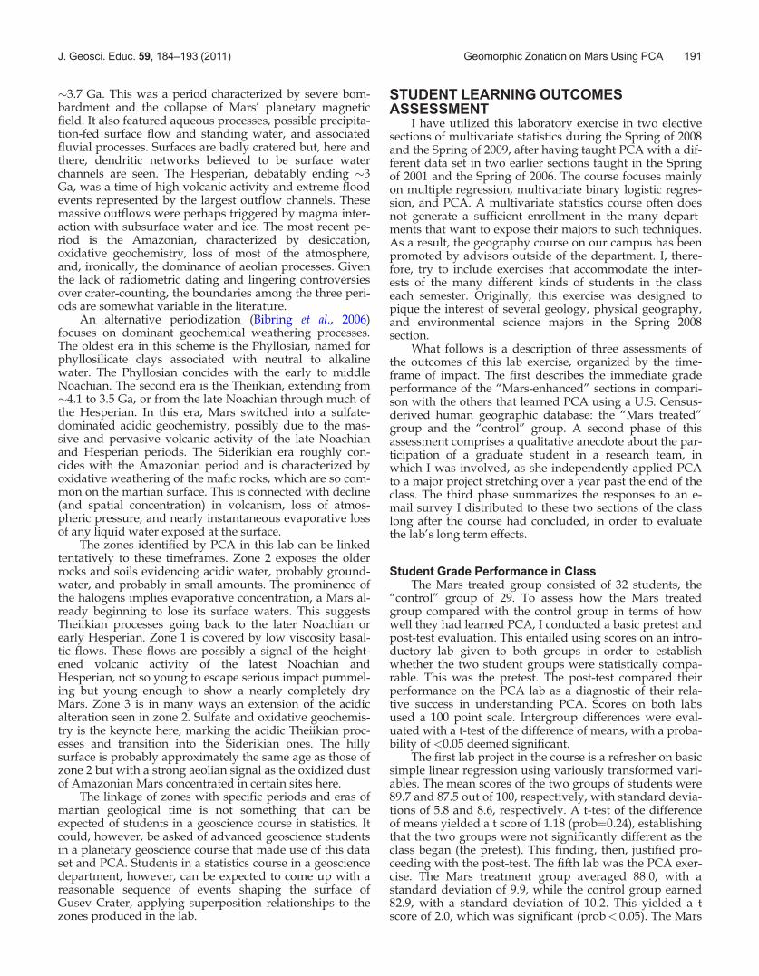
At this point, I have students make one chart with thethree lines corresponding just to the component scores,instead of the variable values (Fig. 1). Students highlightthe sol column and, holding down the control key, sepa-rately tap each of the three component columns in turn aswell. The resulting line chart will be pretty messy, but stu-dents can clean it up by formatting the X axis sol labels torun vertically and the Y axis to have 0 or 1 decimal placesin order to declutter it.

Have the students pay close attention to the first partof Spirit’s traverse and identify which component isdiverging the most strongly upward most of the time andwhich other component is diverging the most stronglydownward. PC2 dominates in the positive direction andPC1 in the negative direction, while PC 3 stays fairly closeto 0. As their eyes move to the right, they will notice that adifferent pair of components diverges most strongly. Thistime PC2 diverges very strongly below neutral and PC3,most of the time, diverges somewhat above neutral, whilePC1, most of the time, stays closest to neutral. At the right-most part of the graph, things change quite drastically,with PC3 diverging very unstably and often with extremevalues below neutral. PC1 shows a similarly spiky positivedominance of most of this area, with PC2, mostly, clingingto neutral. Thus, three zones have been identified by PCA.Students can use the line–draw function (or just a pencil)to sink vertical lines marking the points on the graphwhere the components shift their positive and negativedominance patterns. They should note the sols on whichthese switches take place (roughly sol 158 and sol 315):

TABLE I: Rotated component matrix.

Component

Variable 1 2 3

Na2O 0.772 0.221 0.362

MgO -0.629 -0.573 0.090

Al2O3 0.769 0.306 0.493

SiO2 0.169 -0.011 0.965

P2O5 0.710 0.195 -0.548

SO3 -0.157 -0.140 -0.920

Cl 0.101 -0.870 0.019

K2O 0.751 0.029 0.013

CaO 0.196 0.885 -0.073

TiO2 0.866 0.203 -0.017

Cr2O3 -0.830 0.385 0.121

MnO -0.642 0.571 -0.020

FeO -0.850 0.162 -0.179

Br 0.099 -0.648 -0.232

Ni -0.313 -0.675 -0.009Note: Extraction Method: Principal component analysis, rotation method:Quartimax with Kaiser normalization highest component loading for eachvariable in bold

J. Geosci. Educ. 59, 184–193 (2011) Geomorphic Zonation on Mars Using PCA 187

These mark the boundaries among the three zones, or thesols on which Spirit crossed onto a different kind of terrain.Students are generally pretty impressed by how readilythe landscape is zoned, especially if they had struggled tomake heads or tails of the individual oxide and elementline charts. Now, they can compare this zonation visuallywith the landscape of Gusev Crater.

Turning to a map of Spirit’s traverse <http://marsro-vers.jpl.nasa.gov/mission/tm-spirit/images/MERA_A1457_2_br2.jpg>, as well as a labeled Spirit Pancam image<http://marsrover.nasa.gov/mission/tm-spirit/images/sol_572_in_sol149Pan.jpg>, students should find the twodates marking the boundaries of the three zones. They willfind that the first zone is spatially by far the most exten-sive, a long, almost straight shot across a cratered basalticplain. The second zone is the short curving segmentaround the westernmost spur of the Columbia Hills, a ter-ritory featuring the bedded rocks that the MER team hadoriginally hoped to find when selecting Gusev Crater forSpirit’s landing. The third zone is the ascent into the Co-lumbia Hills, where there proved to be a great diversity ofrock and soil types and team interest sent the rover toexplore this diversity, leading to the very spiky pattern inthe third zone. This third zone, then, foregrounds theteam’s interests perhaps even more than the tenor of theterrain itself.

Depending on time available, faculty can have stu-dents pick out finer scale features, too. Students shouldnote the sols at which components may switch “polarity”or magnitude of scores for brief spells within the threezones and then compare those sols on the traverse mapwith labeled features. In the first zone, for example, stu-dents easily spot the signals of Spirit crossing onto Bonne-ville Crater’s ejecta blanket, then its movement about therim, and then its descent down the blanket toward Mis-soula Crater. The ejecta blanket surface produces speciallymarked and persistent divergences in PC1 and PC2, wherethe impact excavated and ejected deeper basaltic materials.

In the following section, the surface characteristics ofthe three zones emerging from PCA are discussed. The firstzone consists of cratered basaltic plains. The second one of-ten features bedded materials evidencing evaporites. The

third zone is a complex mix of diverse materials suggestiveof acid–aqueous alteration. The discussion section alsoincludes consideration of finer scale subzones in each ofthe three major zones and then finishes with a discussionof processes creating the three main zones.

DISCUSSION OF THE ZONATION PRODUCEDWITH PCA IN GUSEV CRATER

Statistical results and graphs need to be interpretedwithin the concepts of the disciplines generating them.These are challenging enough in this case to require a fairamount of unobtrusive faculty facilitation for students tounderstand. Faculty in geoscience disciplines, for the mostpart, work on Earth, and Mars is peripheral to their normalactivities. There are many excellent books and otherresources to become more comfortable with Mars, but acomprehensive work on the martian surface that includesthe new data from the MER rovers is Carr (2006).

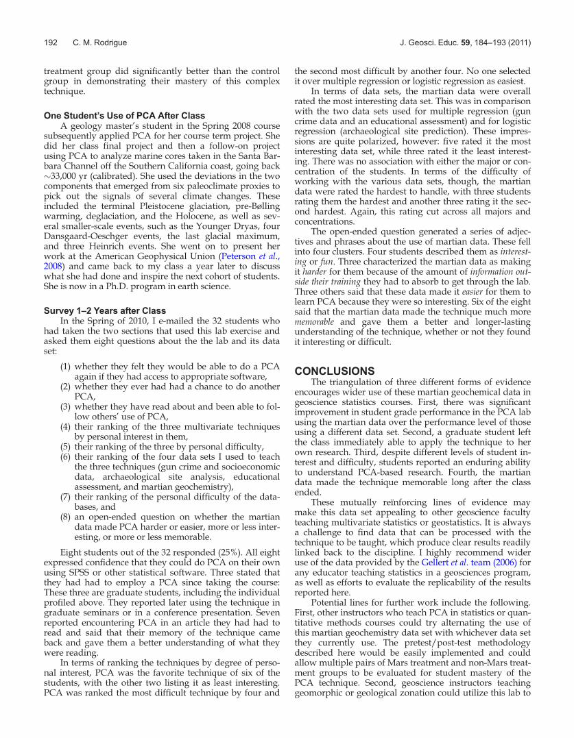
In terms of statistical misunderstandings, it is easy forstudents to interpret negative component scores as “low”scores and positive component scores as “high” scores, forexample. It is important to get across that principal compo-nents are rather like see-saws, with, in this case, differentoxides and elements “seated” on opposite ends of eachcomponent. When the positive side swings up stronglywith highly positive component scores, so do the chemicalsseated on that side (those with positive loadings on thecomponent). Similarly, the negative side can also swing upinto high (negative) component scores, lifting the chemicalswith negative loadings into view. Understanding whichoxides and elements are “lifted into the air” (diverge fromthe neutral 0 component score line in either direction) isimportant for figuring out the nature of the surface. Withthese precautions, Fig. 2 shows Spirit’s transect dividedinto the three zones created by PCA.

Zone 1: Cratered Basaltic PlainSo, in the first zone of Spirit’s transect, PC 1 diverges

strongly in the negative direction. This calls attention to thedominance of ferrous oxide, magnesium oxide, manganeseoxide, and chromium sesquioxide. These oxides indicate

FIGURE 1: PCA factor scores for MER Spirit APXS oxides and elements.

188 C. M. Rodrigue J. Geosci. Educ. 59, 184–193 (2011)

olivines and pyroxenes and other minerals associated withbasalts and the highest temperatures along the reactivebranch of the Bowen reaction series. This component,shifted so far negatively, hints at the lack of aqueous oracid–aqueous alteration along the olivine-to-feldspar join inA-CNK-FM compositional space (Nesbitt and Young, 1989).It also expresses the aeolian deposition of thin coatings ofiron oxides on rock and regolith surfaces. These oxides wereliberated from basalts by the action of atmospheric oxidants,such as hydrogen peroxide. Then, they have been carriedaround the planet by winds to the point of near homogene-ity of global dust composition (Yen et al., 2005).

PC2, meanwhile, diverges very strongly in the positivedirection in this zone, carrying calcium oxide into promi-nence. Since calcium is common in basalts and calcium pla-gioclase dominates the highest temperatures in thenonreactive arm of the Bowen reaction series, the upwardswing of PC2 is not surprising. It reınforces the impressionof a basalt and basaltic regolith landscape dominated byoxides of siderophilic and lithophilic elements. This is thesame signal picked up by the negative swing in PC1.

Zone 2: EvaporitesThe second zone, crossed into by Spirit around sol 158

as it began its exploration of the West Spur of the ColumbiaHills, sees PC2 swing strongly into the negative direction.This carries into prominence the three elements that loadedstrongly onto the negative end of PC2: chlorine, bromine,and nickel. Nickel is associated with certain meteorites, soits presence on any martian surface is not surprising.

Chlorine and bromine, however, are markers of evapo-rative concentration. They were often found within cracksand voids in rocks analyzed by the APXS, starting in thelatter part of zone 1 and then very prominently in zone 2

(Erickson et al., 2005). These two halogens, then, constitutea hint of water or groundwater. This hint counters theimpression of basalts highlighted in the lab’s PCA trendsback in zone 1. Mossbauer spectroscopy on the Spirit roversupports the PCA identification of a mafic surface there.This instrument detects minerals and identified an abun-dance of unaltered or very weakly altered olivine alongGusev’s transect in zone 1 (Morris et al., 2006). Olivine hasa strong proclivity for rapid alteration in the presence ofwater, so its prevalence in the first zone suggests drynessafter the basalt flow event. With the two halogens madeprominent by the negative deviation of PC2, then, this sec-ond zone evidences the presence of small amounts of waterin the older materials outcropping above the basalt surface.These were probably in the form of groundwater or frostdeposition and subsequent aqueous alteration of regolith.

The component most frequently diverging in the posi-tive direction, though not too strikingly, is PC3. The onlychemical to load strongly positively on PC3 is silica. OnEarth, silica can derive from magma fractionation in thecrust or from alteration of basaltic materials through sul-fate geochemistry. Mars had a great deal of sulfur pumpedinto its atmosphere by volcanic activity from �4.2 billionyears ago (Ga) to �3.8 Ga. This was copious enough toproduce geochemical cycles dominated by very acidic sul-fate chemistry. So, these silicas may reflect the “Theiikian”or sulfate era (Bibring et al. 2006; McAdam et al., 2008).

In this region, PC1 occasionally surpasses PC3 in posi-tive deviation, carrying a signal of the oxides of aluminum,sodium, potassium, and titanium. These similarly concen-trate by fractionation but in such minerals as orthoclaseand sodium feldspar. The Spirit team noted that the rockmaterials in zone 2 were softer for the RAT to cut into(Erickson et al., 2005). They commented on a trend of

FIGURE 2: Spirit traverse map showing median component scores and PCA-derived zonation of the traverse fromsols 14 through 470.

J. Geosci. Educ. 59, 184–193 (2011) Geomorphic Zonation on Mars Using PCA 189

increasing detection of small amounts of water alterationin the cratered basaltic plains along the long straight trajec-tory occupying the rover until sol 158. They note that someof the rock appears layered after sol 158, comprising a mixof fine and massive beds, each of which shows relativelypoor size sorting and includes some large grain sizes. Thissuggests deposition in a high energy environment, such asimpact gardening, with subsequent alteration and soften-ing by more water than is evidenced on the basaltic floorof Gusev. This, no doubt, accounts for the change in thepolarity and magnitudes of the three principal componentsmarking the transition from zone 1 to zone 2.

Zone 3: Diversity in Aqueous Sulfate GeochemistryAs Spirit began to climb the northwestern slope of

Husband Hill in the Columbia Hills after sol 315, the land-scape took on a third character geochemically as well astopographically. In this zone, PC3 swings negatively, in acouple of cases quite spectacularly so. Sulfur trioxide is thechemical with a strong negative loading on PC3, bringingup sulfur chemistry again. Sulfate itself (SO4) is not part ofthe database derived from Gellert et al. (2006), but Ericksonet al. (2005) comment that sulfate was abundant in the indi-vidual rocks and soils. This corresponds to the sharp nega-tive deviation in PC3 seen in this lab. Along with the SO3highlighted by PC3’s negative deviation, the sulfates men-tioned by Erickson et al. suggest an aqueous chemistry, thekind associated with the acidic waters produced by sulfategeochemistry (McAdam et al., 2008). Reınforcing theimpression of sulfate chemistry in the third zone are thehalf dozen samples in which PC1 drops sharply into nega-tive scores. Erickson et al. (2005) describe these as basalticgrains cemented by magnesium sulfate salts (the “Peace”and “Alligator” rocks).

It is PC1, however, that diverges strongly positively inmost of the third zone, foregrounding the oxides of tita-nium, sodium, aluminum, potassium, and phosphorous.These are often seen in the granites and rhyolites (quartzand the potassium and sodium feldspars) that result fromthe final fractionation of magmas in the Bowen reaction se-ries, but Mars is not noted for strong magma fractionation.Gellert et al.’s (2006) paper suggests instead that wateracidified by sulfates and chlorine tends not to leach feld-spars with any efficiency. This may account for their pres-ence or persistence in this zone as seen by the felsic oxidesdetected by the APXS, which again underscores acidicaqueous action.

Finer Scale ZonationInstructors might opt to have students tackle finer-

scale zonation as well. Each of the three zones shows sub-zones that depart somewhat from the overall componentpattern in the zone.

In zone 1, for example, the most extreme divergence ofPC1 and PC2 (roughly sols 18–63 and again sols 82–150a)coincides with the ejecta blankets around Bonneville andMissoula craters. Sols 65–81b show a convergence of allthree components toward neutral, which coincides with Spi-rit’s exploration of the rocks along Bonneville Crater’s rim.

In zone 2, students could look for areas that areextremely rich in halogens and carry a suggestion of silica(sols 197–199, 228–235, 300–304). Another subzone typefeatures halogen-rich areas with felsic oxides and the acid–

aqueous alteration they imply (sols 266–274, 291). Studentscan also spot areas close to neutral on all three compo-nents, suggesting aeolian homogenization (sols 172–178,227, 240–259).

In zone 3, students can identify an area of markedalteration toward the oxides of elements common in felsicrocks, with PC1 scores predominantly strongly positive(sols 334–357). Another area adjacent to it has strongly neg-ative PC1 scores. This indicates mafic oxides, and this areaalso shows a weak halogen and sulfate signal from some-what negative PC2 and PC3 scores (sols 374–385b). Imme-diately adjacent is another area in which PC1 scores returnto strongly positive scores but with two rocks showingextremely negative PC3 scores. Scores on these two rocksindicate a very strong sulfate signal (sols 401 and 427).Zone 3 shows the most internal variation of all three zones.This reflects both greater diversity of rocks and soils in theColumbia Hills and the Spirit team’s interests in exploringthe extremes of diversity there.

From Zonation to Processual AnalysisIn short, then, the 15 oxides and elements in this PCA

lab exercise yield three principal components that producea coarse but clear zonation of three different surface typesby geochemistry. These are visually distinct on the Spirittraverse map. If an instructor desires, students can searchfor several finer-scaled subtypes within each zone. Thethree main zones can be turned into a meaningful geosci-ence narrative even by undergraduate students. To do so,they must apply their introductory general geology orphysical geography coursework preparation, which willrequire some facilitation by their faculty. Students shouldhave enough information from their previous courseworkand the lab itself to posit a plausible history along the linesof Mars accreting and forming a crust, followed by a pe-riod of bombardment and impact cratering. During or afterthe bombardment, there was a possibility of fluvial deposi-tion of sediments into Gusev Crater by Ma’adim Vallis.With or without such deposition, there clearly was aque-ous (groundwater?) alteration of impact gardened regolithon the floor of Gusev. After these fluvial and/or aqueousalteration processes had left their marks, volcanic activity(perhaps from Apollinaris Patera to the north of GusevCrater) covered some of these sediments with basaltic lava.This would have been at a time of continued strong bom-bardment, as the basalt is heavily cratered. Bombardmentwent on very heavily until �3.7 Ga and continues at adrastically lower rate even today. The Columbia Hills werestranded as an outcrop of the older water-altered sedi-ments above the younger lava fill. After the volcanic flowevent and after the bombardment of Mars’ surfacedwindled, the long, slow desiccation, oxidation, and aeo-lian homogenization of “modern” Mars began, veneeringrocks and soil with iron oxide dust.

A geological timeline must remain imprecise on Marsuntil the Mars Sample Return Lander and subsequent mis-sions can return rock materials for radiometric dating. Dat-ing of surfaces now depends on crater counting techniques(Hartmann, 2005) and geological reasoning from superpo-sition relationships.

The martian timeline has been divided into three peri-ods (Barlow, 2008), named for region types. The oldest isthe Noachian, which lasted from planetary formation until

190 C. M. Rodrigue J. Geosci. Educ. 59, 184–193 (2011)

�3.7 Ga. This was a period characterized by severe bom-bardment and the collapse of Mars’ planetary magneticfield. It also featured aqueous processes, possible precipita-tion-fed surface flow and standing water, and associatedfluvial processes. Surfaces are badly cratered but, here andthere, dendritic networks believed to be surface waterchannels are seen. The Hesperian, debatably ending �3Ga, was a time of high volcanic activity and extreme floodevents represented by the largest outflow channels. Thesemassive outflows were perhaps triggered by magma inter-action with subsurface water and ice. The most recent pe-riod is the Amazonian, characterized by desiccation,oxidative geochemistry, loss of most of the atmosphere,and, ironically, the dominance of aeolian processes. Giventhe lack of radiometric dating and lingering controversiesover crater-counting, the boundaries among the three peri-ods are somewhat variable in the literature.

An alternative periodization (Bibring et al., 2006)focuses on dominant geochemical weathering processes.The oldest era in this scheme is the Phyllosian, named forphyllosilicate clays associated with neutral to alkalinewater. The Phyllosian concides with the early to middleNoachian. The second era is the Theiikian, extending from�4.1 to 3.5 Ga, or from the late Noachian through much ofthe Hesperian. In this era, Mars switched into a sulfate-dominated acidic geochemistry, possibly due to the mas-sive and pervasive volcanic activity of the late Noachianand Hesperian periods. The Siderikian era roughly con-cides with the Amazonian period and is characterized byoxidative weathering of the mafic rocks, which are so com-mon on the martian surface. This is connected with decline(and spatial concentration) in volcanism, loss of atmos-pheric pressure, and nearly instantaneous evaporative lossof any liquid water exposed at the surface.

The zones identified by PCA in this lab can be linkedtentatively to these timeframes. Zone 2 exposes the olderrocks and soils evidencing acidic water, probably ground-water, and probably in small amounts. The prominence ofthe halogens implies evaporative concentration, a Mars al-ready beginning to lose its surface waters. This suggestsTheiikian processes going back to the later Noachian orearly Hesperian. Zone 1 is covered by low viscosity basal-tic flows. These flows are possibly a signal of the height-ened volcanic activity of the latest Noachian andHesperian, not so young to escape serious impact pummel-ing but young enough to show a nearly completely dryMars. Zone 3 is in many ways an extension of the acidicalteration seen in zone 2. Sulfate and oxidative geochemis-try is the keynote here, marking the acidic Theiikian proc-esses and transition into the Siderikian ones. The hillysurface is probably approximately the same age as those ofzone 2 but with a strong aeolian signal as the oxidized dustof Amazonian Mars concentrated in certain sites here.

The linkage of zones with specific periods and eras ofmartian geological time is not something that can beexpected of students in a geoscience course in statistics. Itcould, however, be asked of advanced geoscience studentsin a planetary geoscience course that made use of this dataset and PCA. Students in a statistics course in a geosciencedepartment, however, can be expected to come up with areasonable sequence of events shaping the surface ofGusev Crater, applying superposition relationships to thezones produced in the lab.

STUDENT LEARNING OUTCOMESASSESSMENT

I have utilized this laboratory exercise in two electivesections of multivariate statistics during the Spring of 2008and the Spring of 2009, after having taught PCA with a dif-ferent data set in two earlier sections taught in the Springof 2001 and the Spring of 2006. The course focuses mainlyon multiple regression, multivariate binary logistic regres-sion, and PCA. A multivariate statistics course often doesnot generate a sufficient enrollment in the many depart-ments that want to expose their majors to such techniques.As a result, the geography course on our campus has beenpromoted by advisors outside of the department. I, there-fore, try to include exercises that accommodate the inter-ests of the many different kinds of students in the classeach semester. Originally, this exercise was designed topique the interest of several geology, physical geography,and environmental science majors in the Spring 2008section.

What follows is a description of three assessments ofthe outcomes of this lab exercise, organized by the time-frame of impact. The first describes the immediate gradeperformance of the “Mars-enhanced” sections in compari-son with the others that learned PCA using a U.S. Census-derived human geographic database: the “Mars treated”group and the “control” group. A second phase of thisassessment comprises a qualitative anecdote about the par-ticipation of a graduate student in a research team, inwhich I was involved, as she independently applied PCAto a major project stretching over a year past the end of theclass. The third phase summarizes the responses to an e-mail survey I distributed to these two sections of the classlong after the course had concluded, in order to evaluatethe lab’s long term effects.

Student Grade Performance in ClassThe Mars treated group consisted of 32 students, the

“control” group of 29. To assess how the Mars treatedgroup compared with the control group in terms of howwell they had learned PCA, I conducted a basic pretest andpost-test evaluation. This entailed using scores on an intro-ductory lab given to both groups in order to establishwhether the two student groups were statistically compa-rable. This was the pretest. The post-test compared theirperformance on the PCA lab as a diagnostic of their rela-tive success in understanding PCA. Scores on both labsused a 100 point scale. Intergroup differences were eval-uated with a t-test of the difference of means, with a proba-bility of <0.05 deemed significant.

The first lab project in the course is a refresher on basicsimple linear regression using variously transformed vari-ables. The mean scores of the two groups of students were89.7 and 87.5 out of 100, respectively, with standard devia-tions of 5.8 and 8.6, respectively. A t-test of the differenceof means yielded a t score of 1.18 (prob¼0.24), establishingthat the two groups were not significantly different as theclass began (the pretest). This finding, then, justified pro-ceeding with the post-test. The fifth lab was the PCA exer-cise. The Mars treatment group averaged 88.0, with astandard deviation of 9.9, while the control group earned82.9, with a standard deviation of 10.2. This yielded a tscore of 2.0, which was significant (prob< 0.05). The Mars

J. Geosci. Educ. 59, 184–193 (2011) Geomorphic Zonation on Mars Using PCA 191

treatment group did significantly better than the controlgroup in demonstrating their mastery of this complextechnique.

One Student’s Use of PCA After ClassA geology master’s student in the Spring 2008 course

subsequently applied PCA for her course term project. Shedid her class final project and then a follow-on projectusing PCA to analyze marine cores taken in the Santa Bar-bara Channel off the Southern California coast, going back�33,000 yr (calibrated). She used the deviations in the twocomponents that emerged from six paleoclimate proxies topick out the signals of several climate changes. Theseincluded the terminal Pleistocene glaciation, pre-Bøllingwarming, deglaciation, and the Holocene, as well as sev-eral smaller-scale events, such as the Younger Dryas, fourDansgaard-Oeschger events, the last glacial maximum,and three Heinrich events. She went on to present herwork at the American Geophysical Union (Peterson et al.,2008) and came back to my class a year later to discusswhat she had done and inspire the next cohort of students.She is now in a Ph.D. program in earth science.

Survey 1–2 Years after ClassIn the Spring of 2010, I e-mailed the 32 students who

had taken the two sections that used this lab exercise andasked them eight questions about the the lab and its dataset:

(1) whether they felt they would be able to do a PCAagain if they had access to appropriate software,

(2) whether they ever had had a chance to do anotherPCA,

(3) whether they have read about and been able to fol-low others’ use of PCA,

(4) their ranking of the three multivariate techniquesby personal interest in them,

(5) their ranking of the three by personal difficulty,(6) their ranking of the four data sets I used to teach

the three techniques (gun crime and socioeconomicdata, archaeological site analysis, educationalassessment, and martian geochemistry),

(7) their ranking of the personal difficulty of the data-bases, and

(8) an open-ended question on whether the martiandata made PCA harder or easier, more or less inter-esting, or more or less memorable.

Eight students out of the 32 responded (25%). All eightexpressed confidence that they could do PCA on their ownusing SPSS or other statistical software. Three stated thatthey had had to employ a PCA since taking the course:These three are graduate students, including the individualprofiled above. They reported later using the technique ingraduate seminars or in a conference presentation. Sevenreported encountering PCA in an article they had had toread and said that their memory of the technique cameback and gave them a better understanding of what theywere reading.

In terms of ranking the techniques by degree of perso-nal interest, PCA was the favorite technique of six of thestudents, with the other two listing it as least interesting.PCA was ranked the most difficult technique by four and

the second most difficult by another four. No one selectedit over multiple regression or logistic regression as easiest.

In terms of data sets, the martian data were overallrated the most interesting data set. This was in comparisonwith the two data sets used for multiple regression (guncrime data and an educational assessment) and for logisticregression (archaeological site prediction). These impres-sions are quite polarized, however: five rated it the mostinteresting data set, while three rated it the least interest-ing. There was no association with either the major or con-centration of the students. In terms of the difficulty ofworking with the various data sets, though, the martiandata were rated the hardest to handle, with three studentsrating them the hardest and another three rating it the sec-ond hardest. Again, this rating cut across all majors andconcentrations.

The open-ended question generated a series of adjec-tives and phrases about the use of martian data. These fellinto four clusters. Four students described them as interest-ing or fun. Three characterized the martian data as makingit harder for them because of the amount of information out-side their training they had to absorb to get through the lab.Three others said that these data made it easier for them tolearn PCA because they were so interesting. Six of the eightsaid that the martian data made the technique much morememorable and gave them a better and longer-lastingunderstanding of the technique, whether or not they foundit interesting or difficult.

CONCLUSIONSThe triangulation of three different forms of evidence

encourages wider use of these martian geochemical data ingeoscience statistics courses. First, there was significantimprovement in student grade performance in the PCA labusing the martian data over the performance level of thoseusing a different data set. Second, a graduate student leftthe class immediately able to apply the technique to herown research. Third, despite different levels of student in-terest and difficulty, students reported an enduring abilityto understand PCA-based research. Fourth, the martiandata made the technique memorable long after the classended.

These mutually reınforcing lines of evidence maymake this data set appealing to other geoscience facultyteaching multivariate statistics or geostatistics. It is alwaysa challenge to find data that can be processed with thetechnique to be taught, which produce clear results readilylinked back to the discipline. I highly recommend wideruse of the data provided by the Gellert et al. team (2006) forany educator teaching statistics in a geosciences program,as well as efforts to evaluate the replicability of the resultsreported here.

Potential lines for further work include the following.First, other instructors who teach PCA in statistics or quan-titative methods courses could try alternating the use ofthis martian geochemistry data set with whichever data setthey currently use. The pretest/post-test methodologydescribed here would be easily implemented and couldallow multiple pairs of Mars treatment and non-Mars treat-ment groups to be evaluated for student mastery of thePCA technique. Second, geoscience instructors teachinggeomorphic or geological zonation could utilize this lab to

192 C. M. Rodrigue J. Geosci. Educ. 59, 184–193 (2011)

do a similar comparison of “PCA treated” and “non-PCAtreated” student groups. They could evaluate whether ex-posure to PCA promotes a better understanding of zona-tion in comparison with other techniques, such as fieldobservation, air photo interpretation, or software-mediatedclassification of remote sensing data. Construction of ashared assessment data clearinghouse on either of thesetopics could facilitate curricular development in geosciencedepartments. Such a clearinghouse could be made publicthrough the Digital Library for Earth System Education(DLESE) or the Education Resources Information Center(ERIC).

REFERENCESBaker, G.S., and Jol, H.M. (ed.), 2007., Stratigraphic analyses using

GPR: Boulder, CO, Geological Society of America, special pa-per 432, 183 p.

Barlow, N., 2008, Mars: An introduction to its interior surface,and atmosphere: Cambridge, U.K., Cambridge UniversityPress, 264 p.

Bibring, J.-P., Langevin, Y., Mustard, J.F., Poulet, F., Arvidson, R.,Gendrin, A., Gondet, B., Mangold, N., Pinet, P., Forget, F.,and the OMEGA team, 2006, Global mineralogical and aque-ous Mars history derived from OMEGA/Mars Express data:Science v. 312, p. 400–404.

Brown, K.J., and Pasternack, G.B., 2004, The geomorphic dynam-ics and environmental history of an upper deltaic floodplaintract in the Sacramento-San Joaquin Delta, California, USA:Earth Surface Processes and Landforms, v. 29, p. 1235–1258.

Bryant, F.B., and Yarnold, P.R., 1995, Principal-components anal-ysis and exploratory and confirmatory factor analysis, inGrimm, L.G. and Yarnold, P.R., editors,. Reading and under-standing multivariate statistics: Washington, D.C., AmericanPsychological Association, p. 99–136.

Bushnell, T.M., 1942, Some aspects of the soil catena concept: SoilScience Society of America Proceedings, v. 7, p. 466–476.

Carr, M.H., 2006, The surface of Mars: Cambridge, U.K., Cam-bridge University Press, 307 p.

Dark, S.J., and Bram, D., 2007, The modifiable areal unit problem(MAUP) in physical geography: Progress in Physical Geogra-phy, v. 31, p. 471–479.

Davis, J.C., 2002, Statistics and data analysis in geology, 3rd ed.:New York, Wiley, 638 p.

Erickson, J.K., Callas, J.L., and Haldemann, A.F.C., 2005, TheMars Exploration Rover Project: 2005 surface operationsresults. Paper presented to the 56th International Astronomi-cal Congress, Fukuoka, Japan, October 17–21 Available athttp://trs-new.jpl.nasa.gov/dspace/bitstream/2014/39527/1/05-2706.pdf.

Fortin, M.-J., Olson, R.J., Ferson, S., Iverson, L., Hunsaker, C.,Edwards, G., Levine, D., Butera, K., and Klemas, V., 2000,Issues related to the detection of boundaries: Landscape Ecol-ogy, v. 15, p. 453–466.

Hartmann, W.K., 2005, Martian cratering 8: Isochron refinementand the chronology of Mars: Icarus, v. 174, p. 294–320.

Gellert, R., Rieder, R., Bruckner, J., Clark, B.C., Dreibus, G., Klin-gelhofer, G., Lugmair, G., Ming, D.W., Wanke, H., Yen, A.,Zipfel, J., and Squyres, S.W., 2006, Alpha particle x-ray spec-trometer (APXS): Results from Gusev crater and calibration

report: Journal of Geophysical Research (Planets), v. 111, p.E02S05.

Imbrie, J., and Van Andel, T.J., 1964, Vector analysis of heavy-mineral data: Geological Society of America Bulletin, v. 75, p.1131–1155.

McAdam, A.C., Zolotov, M.Y., Mironenko, M.V., and Sharp,T.B., 2008, Formation of silica by low-temperature acidalteration of Martian rocks: Physical-chemical constraints:Journal of Geophysical Research, v. 113, p. E08003.

Milne, G., 1935, Some suggested units of classification and map-ping particularly for East African soils: Soil Research, v. 4, p.183–198.

Morris, R.V., Klingelhofer, G., Schroder, C., Rodionov, D.S., Yen,A., Ming, D.W., de Souza, Jr., P.A., Fleischer, I., Wdoviak, T.,Gellert, R., Bernhardt, B., Evlanov, E.N., Zubkov, B., Foh, J.,Bonnes, U., Kankeleit, E., Gutlich, P., Renz, F., Squyres, S.,and Arvidson, R.E., 2006, Mossbauer mineralogy of rock,soil, and dust at Gusev crater, Mars: Spirit’s journey throughweakly altered olivine basalt on the plains and pervasivelyaltered basalt in the Columbia Hills: Journal of GeophysicalResearch (Planets), v. 111, p. E02S13.

Nesbitt, H.W., and Young, G.M., 1989, Formation and diagensisof weathering profiles: Journal of Geology, v. 97, p. 129–147.

Patterson, R.T., Hutchinson, I., Guilbault, J.-P., and Clague, J.J.,2000, A comparison of the vertical zonation of diatom, fora-minifera, and macrophyte assemblages in a coastal marsh:Implications for greater paleo-sea level resolution: Micropa-leontology, v. 46, p. 229–244.

Peterson, C.D., Behl, R.J., Rodrigue, C.M., Zeleski, C.M., and Hill,T.M., 2008, Statistical relationships among proxies of climate,productivity, and the carbon cycle across climatic regimes,Santa Barbara Basin, California: American GeophysicalUnion, Fall Meeting, San Francisco, California, PP51C-1508.

Raynolds, M.A., Walker, D.A., and Maier, H.A., 2006, Alaska arc-tic tundra vegetation map. Scale 1:4,000,000: U.S. Fish andWildlife Service, Anchorage, Alaska, Habitats along a meso-topographic gradient, p. 2.

Reyment, R.A. 1961, Quadrivariate principal components analysisof Globigerina Yeguaensis: Stockholm Contributions in Geol-ogy, v. 8, p. 17–26.

Rogerson, P.A., 2006, Statistical methods for geography: A stu-dent’s guide: London, Sage, 304 p.

Taylor, R.B., 2010, Communities, crime, and reactions to crimemultilevel models: Accomplishments and meta-challenges:Journal of Quantitative Criminology, v. 26, p. 455–466.

Webster, R., 1973, Automatic soil-boundary location from transectdata: Mathematical Geology, v. 5, p. 27–37.

Wong, S.T., 1963, A multivariate statistical model for predictingmean annual flood in New England: Annals of the Associa-tion of American Geographers, v. 53, p. 298–311.

Yen, A.S., Gellert, R., Schroder, C., Morris, R.V., Bell, III, J.F.,Knudson, A.T., Clark, B.C., Ming, D.W., Crisp, J.A., Arvid-son, R.E., Blaney, D., Bruckner, J., Christensen, P.R., DesMar-ais, D.J., de Souza, Jr., P.A., Economou, T.E., Ghosh, A.,Hahn, B.C., Herkenhoff, K.E., Haskin, L.A., Hurowitz, J.A.,Joliff, B.L., Johnson, J.R., Klingelhofer, G., Madsen, M.B.,McLennan, S.M., McSween, H.Y., Richter, L., Rieder, R.,Rodionov, D., Soderblom, L., Squyres, S.W., Tosca, N.J.,Wang, A., Wyatt, M., and Zipfel, J., 2005, An integrated viewof the chemistry and mineraology of martian soils: Nature,v. 436, p. 49–54.

J. Geosci. Educ. 59, 184–193 (2011) Geomorphic Zonation on Mars Using PCA 193