U.S. NO2 trends (2005–2013): EPA Air Quality System1

(AQS) data versus improved observations from the2

Ozone Monitoring Instrument (OMI)3

Lok N. Lamsala,b,∗, Bryan N. Duncanb, Yasuko Yoshidac,b, Nickolay A.4

Krotkovb, Kenneth E. Pickeringb, David G. Streetsd, Zifeng Lud5

aGoddard Earth Sciences Technology and Research, Universities Space Research6

Association, Columbia, MD, USA7

bNASA Goddard Space Flight Center, Greenbelt, MD, USA8

cScience Systems and Applications, Inc., MD, USA9

dDecision and Information Sciences Division, Argonne National Laboratory, Argonne,10

IL, USA11

Abstract12

Emissions of nitrogen oxides (NOx) and, subsequently, atmospheric levels13

of nitrogen dioxide (NO2) have decreased over the U.S. due to a combination14

of environmental policies and technological change. Consequently, NO2 levels15

have decreased by 30–40% in the last decade. We quantify NO2 trends (2005–16

2013) over the U.S. using surface measurements from the U.S. Environmental17

Protection Agency (EPA) Air Quality System (AQS) and an improved tro-18

pospheric NO2 vertical column density (VCD) data product from the Ozone19

Monitoring Instrument (OMI) on the Aura satellite. We demonstrate that20

the current OMI NO2 algorithm is of sufficient maturity to allow a favorable21

correspondence of trends and variations in OMI and AQS data. Our trend22

model accounts for the non-linear dependence of the NO2 concentration on23

emissions associated with the seasonal variation of the chemical lifetime, in-24

cluding the change in the amplitude of the seasonal cycle associated with25

∗Corresponding author

Email address: lok.lamsal@nasa.gov (Lok N. Lamsal)Preprint submitted to Atmospheric Environment February 2, 2015

the significant change in NOx emissions that occurred over the last decade.26

The direct relationship between observations and emissions becomes more27

robust when one accounts for these non-linear dependencies. We improve28

the OMI NO2 standard retrieval algorithm and, subsequently, the data prod-29

uct by using monthly vertical concentration profiles, a required algorithm30

input, from a high-resolution chemistry and transport model (CTM) sim-31

ulation with varying emissions (2005–2013). The impact of neglecting the32

time-dependence of the profiles leads to errors in trend estimation, particu-33

larly in regions where emissions have changed substantially. For example, we34

find that by including the time-dependency there are 18% more instances of35

significant trends and up to 15% larger total NO2 reduction. Using a CTM,36

we explore the theoretical relation of the trends estimated from NO2 VCDs37

to those estimated from ground-level concentrations. The model-simulated38

trends in VCDs strongly correlate with those estimated from surface concen-39

trations (r = 0.83, N = 355). We then explore the observed correspondence40

of trends estimated from OMI and AQS data. We find a significant, but41

slightly weaker, correspondence (i.e., r = 0.68, N = 208) than predicted by42

the model and discuss some of the important factors affecting the relation-43

ship, including known problems (e.g., NOz interferents) associated with the44

AQS data. This significant correspondence gives confidence in trend and45

surface concentration estimates from OMI VCDs for locations, such as the46

majority of the U.S. and globe, that are not covered by surface monitoring47

networks. Using our improved trend model and our enhanced OMI data48

product, we find that both OMI and AQS data show substantial downward49

trends from 2005 to 2013, with an average reduction of 38 % for each over50

2

the U.S. The annual reduction rates inferred from OMI and AQS measure-51

ments are larger (-5.0 %/yr, -3.7 %/yr) from 2005 to 2008 than 2010 to 201352

(-1.6 %/yr, -2.8 %/yr). We quantify NO2 trends for major U.S. cities and53

power plants; the latter suggest the largest trend (-4 %/yr) by 2008 and54

small or insignificant changes during 2010–2013.55

Keywords: Nitrogen dioxide, troposphere, air quality, trend, Aura OMI56

1. Introduction57

Emissions of nitrogen oxides (NOx = NO + NO2) are regulated by the58

U.S. Environmental Protection Agency (EPA), because NOx contributes to59

the formation of unhealthy levels of surface ozone, a pollutant that has been60

long known to damage lung tissue when inhaled (Kleinfield et al., 1957;61

Challen et al., 1958). Though nitrogen dioxide (NO2) is a respiratory ir-62

ritant, its levels in the U.S. are currently below the National Ambient Air63

Quality Standard (NAAQS) set by EPA (EPA, 2008). As a result of emis-64

sion reductions from mobile and point sources (e.g., McDonald et al., 2012;65

Xing et al., 2013), surface NO2 levels in the U.S. decreased by 33 % between66

2001 and 2010 and, subsequently, ozone concentrations decreased by 14 %,67

when year-to-year variations in meteorology are taken into account (EPA,68

2012). The temporal evolution of this substantial decrease in NO2 has been69

recorded by the Ozone Monitoring Instrument (OMI), which was launched on70

the NASA Aura satellite in July 2004 (Figure 1). In this manuscript, we show71

that recent modifications to the OMI retrieval algorithm have sufficiently im-72

proved the quality of the data product so that trends and variations derived73

from OMI and EPA Air Quality System (AQS) surface data are similar for74

3

2005 2013

0.1 0.9 1.8 2.7 3.6 4.5 5.4 6.3 x 1015 [molec. cm-2]

Figure 1: Annual average OMI tropospheric NO2 VCDs at 1/2 latitude × 2/3 longitude

spatial resolution for 2005 (left) and 2013 (right).

U.S. cities.75

Tropospheric vertical column density (VCD) data of NO2, as measured76

from space, serve as an effective proxy for surface NO2 in many air quality77

applications. (The VCD is defined as the number of molecules of an at-78

mospheric gas between the satellite instrument and the Earth′s surface per79

unit area.) For instance, VCD data are used for inferring surface NOx emis-80

sions (Leue et al., 2001; Martin et al., 2003; Jaegle et al., 2005; Wang et al.,81

2007; Boersma et al., 2008a; Napelenok et al., 2008; Zhao and Wang, 2009;82

Lin et al., 2010; Lamsal et al., 2011; Streets et al., 2013; Tang et al., 2013;83

Ghude et al., 2013; Vinken et al., 2014), estimating trends and variations84

in atmospheric concentrations (Beirle et al., 2003; Richter et al., 2005; Frost85

et al., 2006; Boersma et al., 2008b; Lin and McElroy, 2011; Zhou et al., 2012;86

Castellanos and Boersma, 2012; Russell et al., 2012), monitoring emission87

changes in point sources (e.g., Kim et al., 2006; Wang et al., 2012; Duncan88

4

et al., 2013), and inferring ozone formation sensitivities to NOx and VOCs89

levels (Martin et al., 2004; Duncan et al., 2010; Valin et al., 2013; Tang et al.,90

2014). Duncan et al. (2013) demonstrated that variations and trends in OMI91

NO2 data near US power plants correlate well with changes in emissions re-92

ported by the Continuous Emissions Monitoring System (CEMS) for large93

facilities, particularly if they are located away from cities. Lamsal et al.94

(2008, 2010) used an early version of OMI NO2 data to infer ground-level95

concentrations, such as those measured by the EPA AQS network, over a96

range of locations and seasons. They found that their OMI-derived surface97

concentrations, estimated using a chemistry and transport model (CTM),98

were significantly correlated with AQS observations, both temporally and99

spatially, though the correlations varied widely between monitoring stations.100

The EPA AQS network of surface monitors is sparse and unevenly dis-101

tributed, including in major metropolitan areas. The network lacks observa-102

tions for large regions of the U.S. Because the lifetime of NOx is short, trends103

estimated from these monitoring data may not be spatially representative,104

confounding NO2 trend estimates derived from these surface data. Moreover,105

NO2 trends estimated from the commonly used chemiluminescent monitor106

(equipped with molybdenum oxide converter) data may differ from true NO2107

trends because of interference from the oxidation products of NOx (NOz),108

such as peroxyacetyl nitrate (PAN), alkyl nitrates, and nitric acid (HNO3)109

(Winer et al., 1974; Dunlea et al., 2007; Steinbacher et al., 2007; Lamsal110

et al., 2008). Satellite observations, which have the advantage of spatial cov-111

erage, provide information on NO2-specific trends, which complement and112

enrich the AQS-observed trends. Here, we take advantage of three indepen-113

5

dent measurements from OMI, a photolytic converter, and a molybdenum114

converter to explore (1) how trends derived from OMI measurements, which115

are collocated once per day, relate to trends available from high temporal res-116

olution (hourly) surface data, and (2) how the interference in molybdenum117

converter measurements could affect the actual observed NO2 trend.118

In this manuscript, we conduct a systematic investigation of the relation-119

ship between AQS and OMI NO2 trends; to our knowledge, such a trend120

estimation and comparison have not been shown before. In Section 2, we de-121

scribe our method for estimating trends, our new high-resolution OMI VCD122

data product and the surface data that we use in our analysis. We also123

present a model study of the expected correspondence of trends derived from124

VCD and surface concentration data and discuss the various factors that125

should be considered when comparing these trends. We discuss the observed126

correspondence of trends derived from OMI VCD and AQS data in Section 3.127

We summarize our conclusions in Section 4.128

2. Observations, model and methods129

2.1. Multivariate linear regression for trend estimation130

We use a regression model to infer both the seasonal and the linear trend131

components in OMI and AQS NO2 observations. The time series of monthly132

average NO2 values (Ω) can be assumed to be comprised of three additive133

subcomponents: a time dependent seasonal component (α), a linear trend134

component (β), and residual or noise (R) component:135

Ω(t) = α(t) + β(t) + R(t), (1)

6

where t represents time (month). The time dependent regression component136

(α) is given by a constant plus intra-annual sine and cosine harmonic series137

(Randel and Cobb, 1994):138

α(t) = c0 +3∑

j=1

(c1j sin(2πjt

12) + c2j cos(

2πjt

12)), (2)

where c0, c1j, and c2j are constant coefficients to be determined from the139

measurements. The major portion of the NO2 annual cycle is explained by140

the seasonal variation of the NOx lifetime. The contributions from all other141

factors, such as monthly variation in NOx emissions, to the seasonal cycle142

are typically small. The seasonal pattern may be constant or evolve in time.143

Analysis of the temporal evolution of the seasonal variation of OMI NO2144

over the eastern U.S. reveals a considerable change (decrease) in seasonal145

amplitude over the Aura record, suggesting the need of an approach that146

accounts for it when calculating the trend and estimating trends in emis-147

sions. Changes in the seasonal amplitude are also reported by Hilboll et al.148

(2013) and occur at places where NOx emissions are changing rapidly due to149

economic growth or emission control measures. Removal of varying seasonal150

components in a time series can be achieved by a locally weighted regression151

smoothing technique (Cleveland et al., 1990) or by including a scaling factor152

(Hilboll et al., 2013). In line with these methods, we identify and extract153

seasonal and linear trend components by exploiting changes in the measured154

seasonal pattern (amplitude and phase) for individual years. For each year,155

Y, we fit a regression line using monthly observations from that year it-156

self plus 6 monthly observations from years adjacent to Y. This provides a157

series of local regression lines, which incorporate explicit time dependence.158

7

Comparison of local regression lines with high- and low-amplitude regression159

lines allows identification and isolation of two seasonal terms (α1, α2, where160

α = α1 + α2 in Eq. 1 and α1 represents the regression line with the lowest161

seasonal amplitude) and the linear trend (β). A graphical illustration of ap-162

plying the multiple regression analysis to OMI data is shown in Figure A1163

in AppendixA.164

2.2. The expected correspondence of NO2 VCDs and surface concentrations165

As mentioned in Section 1, the primary advantage of satellite data for es-166

timating trends is spatial coverage, especially for areas without surface mon-167

itors or ones where the existing monitors do not provide NO2 levels or trends168

that are representative of an urban area as discussed in Section 2.4.3. In ad-169

dition, a VCD has the advantage over surface data that it also includes NO2170

above the surface, which is necessary for estimating variations and trends171

in NOx levels and emissions from all sources, including power plants where172

emissions are released well above the surface (i.e., tall smokestacks and plume173

rise).174

We use the NASA Global Modeling Initiative (GMI) CTM, which is de-175

scribed in AppendixB, to examine how the trend in surface level NO2 ob-176

served by AQS relates to the trend in OMI VCD data. We examine the177

observed correspondence in Section 3.1. The simulation includes annually178

varying anthropogenic emissions and captures both the spatial distribution179

and temporal changes observed by OMI over the continental U.S. (Strode180

et al., 2014).181

We apply the multivariate linear regression analysis, described in Sec-182

tion 2.1, to the model output to calculate the linear trend component (β)183

8

0 10 20 30 40 50Reduction in surface NO2 [%]

0

10

20

30

40

50

Red

uctio

n in

trop

osph

eric

NO

2 VC

D [%

]

r = 0.83, N = 355

1.0 1.9 2.8 3.7 4.6 5.5 6.4 7.4

Tropospheric NO2 VCD [1015 molec. cm-2], 2005

Figure 2: Model simulated reduction (%, 2005–2010) in surface NO2 versus reduction

in tropospheric NO2 VCDs. Reductions in VCDs are color-coded by tropospheric NO2

VCDs for 2005. The results are from a GMI simulation over the U.S., and include only

areas with annual average tropospheric NO2 VCDs > 1× 1015 molecules cm−2 and statis-

tically significant trends at the 95 % confidence level. The dotted line represents the 1:1

relationship.

in surface concentrations and tropospheric VCDs. Figure 2 compares the184

reductions (calculated from β) for 2005–2010 in surface NO2 with those in185

tropospheric NO2 VCDs over all polluted areas in the U.S. The trend in186

surface concentrations is well correlated (r = 0.83, N = 355) with the trend187

in VCDs, though, as expected, the scatter is higher for lower VCDs as the188

contribution of surface NO2 to the tropospheric VCD is less than in polluted189

areas. The reductions in surface concentrations range from 6.4 to 42 %, while190

tropospheric VCD reductions range from 8.6 to 41 %. Reductions are higher191

over power plants in the tropospheric VCDs than the surface concentrations192

9

because of tall smokestacks and plume rise associated with these sources.193

The average reductions for the two quantities are in agreement to within194

4 %, but their correlation improves with increasing NO2 levels (Figure 2).195

2.3. Description of OMI observations and recent improvements relevant for196

U.S. air quality applications197

2.3.1. Retrievals of tropospheric NO2 VCD198

The OMI monitors NO2 VCDs by measuring spectral variation in backscat-199

tered solar radiation in the broad visible spectral window between 405 nm200

and 465 nm. OMI measurements are made in early afternoon (i.e., local time201

of 13:00–14:45) with a spatial resolution of 13 × 24 km2 at nadir and with202

nearly daily global coverage.203

In this work, we further improve the operational OMI NO2 retrieval algo-204

rithm (NASA standard Product, version 2.1 see AppendixC), by using new a205

priori NO2 profiles simulated by the GMI CTM with year-specific emissions.206

The profiles not only improve the representation of the NO2 vertical distri-207

bution, but also capture the yearly changes in NO2 profile shapes. The latter208

is critical due to rapid decline in the U.S. NOx emissions in recent years (e.g.,209

Figure 1), as NO2 retrievals and, therefore, the estimated trends are sensitive210

to the vertical shape of NO2 profiles as discussed in Section 2.3.2.211

We use individual pixel clear sky (cloud radiance fraction < 0.5) Level 2212

OMI NO2 data. The estimated errors in individual tropospheric NO2 VCDs213

observed under polluted (tropospheric NO2 VCD > 1×1015 molecules cm−2)214

and clear sky conditions are ∼30 % (Bucsela et al., 2013). To exclude the215

cross-track rows affected by the row anomaly after 2007 and to avoid incon-216

sistent sampling, we use OMI data for rows 5–23 for the entire OMI dataset.217

10

The largest pixels that are at swath edges (rows 1–4) were excluded to reduce218

spatial smearing of tropospheric NO2. We then map the remaining data into219

a 0.1 latitude × 0.1 longitude grid by calculating an area-weighted aver-220

age. The approach accounts for the overlap and size of OMI ground footprints221

(pixels). Finally, we compute monthly averages to estimate trends for the222

entire OMI period (2005–2013).223

2.3.2. Impact on the OMI-derived trend of the assumption of the vertical224

NO2 distribution in the retrieval algorithm225

Satellite retrieval algorithms of NO2 VCDs are sensitive to the assumed226

vertical distribution of NO2 (Martin et al., 2002; Boersma et al., 2004; Heckel227

et al., 2011; Russell et al., 2011; Hains et al., 2010; Lamsal et al., 2014). Most228

operational NO2 retrieval algorithms assume an a priori vertical distribution,229

such as those taken from a coarse-resolution CTM (e.g. Boersma et al., 2011;230

Hilboll et al., 2013; Bucsela et al., 2013). Since the model simulations often231

use outdated bottom-up emissions, these profiles may not capture the actual232

vertical distribution of NO2, especially where anthropogenic NOx emissions233

are undergoing rapid changes (e.g., Figure 1). For instance, the operational234

OMI retrieval algorithm (NASA standard product, version 2.1) uses a cli-235

matology of a priori NO2 profiles at 2 latitude × 2.5 longitude horizontal236

resolution from a GMI CTM simulation based on emissions from the 1999237

National Emission Inventory (NEI). Here, we explore how the current prac-238

tices of operational algorithms employing NO2 profiles based on constant239

and/or outdated emissions affect satellite-derived NO2 trends.240

As discussed in Section 2.3.1, we performed two separate retrievals, one241

using monthly NO2 vertical profiles based on emissions and meteorology of242

11

2005 profiles Year-specific profiles

4842363024181260 [%]

2005-2010 reduction

0 10 20 30 40 50 602005-2010 reduction [%]

-15

-10

-5

0

5

Diff

eren

ce in

red

uctio

n [%

]

0.0 0.9 1.8 2.7 3.6 4.5 5.4 6.4

Tropospheric NO2 VCD [1015 molec cm-2]

Figure 3: Percent reduction in OMI tropospheric NO2 VCDs for 2005–2010 (1/2 latitude

× 2/3 longitude horizontal resolution) calculated from two separate retrievals, one using

2005 (left) and another using year-specific (middle) monthly mean NO2 vertical profiles.

The dark gray color represents the locations with insignificant trends at 95 % confidence.

(right) The difference between trends calculated from the retrievals based on 2005 profiles

minus the retrievals based on year-specific profiles. Values are color-coded by average

tropospheric NO2 VCDs for 2005.

2005, which we refer to as “2005 profiles”, and another using monthly NO2243

profiles based on year-specific emissions and meteorology, which we refer244

to as “year-specific profiles”, to demonstrate the impact of vertical profile245

assumptions on the OMI-derived NO2 trends. Interannual variations in the246

meteorological fields are expected to have a minor effect on monthly average247

NO2 data. We use OMI pixels with cloud radiance fraction < 0.5, calculate248

area-weighted average VCDs on a 1/2 latitude × 2/3 longitude horizontal249

grid, and use Eq. 1 to derive linear trends for 2005–2010.250

Figure 3 shows the spatial variation of NO2 reduction for 2005–2010 cal-251

culated from the two retrievals. Although the reductions from both retrievals252

are highly consistent with one another (r = 0.97, N = 3524), the year-specific253

retrievals offer a considerably higher number (18 %) of cases with significant254

12

trends and up to 15 % larger reductions. Therefore, using 2005 profiles in255

the retrievals underestimates the trends, on average, by 0.6 %/yr and overall256

2005–2010 reduction by 3.5 %. The smaller deviations for larger VCDs imply257

that the trend is less sensitive to the vertical profile assumption in highly258

polluted areas. Since the vertical profiles used in the generation of OMI op-259

erational products are based on NEI 1999, we anticipate that annual trends260

estimated using these products would be biased low.261

2.4. Description of in situ surface NO2 measurements and considerations for262

trend estimation263

2.4.1. AQS surface measurements264

We use hourly NO2 measurements from the EPA AQS monitoring net-265

work (Demerjian, 2000). The network employs the EPA-designated NO2266

chemiluminescence automated Federal Reference Method (FRM) described267

in detail in EPA (1975). The NO2 measurement method of these commercial268

instruments relies on detecting NO by reducing NO2 to NO on the surface of269

a heated molybdenum oxide (MoOx) substrate at 300–400C. However, the270

reduction of NO2 to NO by the MoOx substrate is not specific to NO2, but is271

also sensitive to some unknown fraction of NOz (NOz′) (Winer et al., 1974;272

Grosjean and Harrison, 1985; Demerjian, 2000; EPA, 2006; Dunlea et al.,273

2007; Steinbacher et al., 2007; Lamsal et al., 2008). The magnitude of the274

total interference is variable, and depends not only on the relative fraction of275

actual NO2 to total reactive nitrogen compounds (NOy = NOx + NOz), but276

also on the characteristics of individual monitors. As a result, NO2 measure-277

ments from AQS monitors are consistently biased high (up to 50 %), with278

the highest biases in the afternoon as discussed in Section 2.4.2, at distant279

13

locations from NOx sources, and during summer months when these NOz280

products are expected to peak (e.g., Steinbacher et al., 2007). The Aura281

overpass is once per day in early afternoon when this bias is near its daily282

maximum.283

To relate OMI with AQS observations, we select measurements collocated284

in space and time. For overlapping OMI overpasses for a given day, we285

compute averages weighted by OMI ground pixel sizes. The hourly data286

from AQS are averaged over a 2-hour period (13:00–15:00 local time) to287

temporally match with the OMI measurements. We exclude stations that288

offer measurements only during the summer ozone season or ceased operation289

anytime between 2005 and 2013. These criteria retain 208 sites, including290

30 in rural, 89 in suburban, and 88 in urban environments. We also use the291

hourly data from these sites to examine the diurnal variation in surface NO2292

trends in Section 4.293

2.4.2. Interferences in the AQS-observed trends294

Here we examine how the trend estimated from the biased AQS NO2 data295

relates to the actual NO2 trend. We use hourly NO2 observations made by296

collocated MoOx and more accurate photolytic converter instruments at a297

rural site in Yorkville, Georgia, which is located 72 km to the northwest of298

Atlanta. The photolytic converter instrument employs broadband photolysis299

of ambient NO2 followed by chemiluminescence detection of the product,300

NO, offering a true NO2 measurement with accuracy better than 10 % (Kley301

and McFarland, 1980; Ryerson et al., 2000; Zellweger et al., 2000; Pollack302

et al., 2010). Long-term photolytic converter measurements are available303

from the SouthEastern Aerosol Research and Characterization (SEARCH)304

14

01

2

3

4

5

6

NO

2 [ppb

]

PhotolyticMolybdenum 2005

2010

1.0

1.2

1.4

1.6

Mol

ybde

num

/Pho

toly

tic 20052010

Time of day

20

30

40

50

60

70

2005

-201

0 re

duct

ion

[%]

PhotolyticMolybdenum

00 01 02 03 04 05 06 07 08 09 10 11 12 13 14 15 16 17 18 19 20 21 22 23

Figure 4: (top) Hourly averaged surface NO2 mixing ratios for 2005 (red) and 2010 (blue)

measured by collocated AQS molybdenum (dotted line open circles) and SEARCH pho-

tolytic (solid line with closed circles) converter analyzers at Yorkville, GA. (middle) Hourly

variations of the ratio of the molybdenum and photolytic measurements for 2005 and 2010.

(bottom) Diurnal changes in the NO2 reductions for 2005–2010 calculated from the pho-

tolytic and molybdenum converter measurements.

network (Edgerton et al., 2006). We use the data for the period 2005–2010305

to calculate annual averages and monthly trends.306

Figure 4 (top) shows the diurnal variation of annually averaged NO2307

measured by the MoOx converter and photolytic converter instruments. The308

two measurements agree to within 5 % between 8 PM and 8 AM in 2005.309

Significant differences of 8–43 % are observed during the day with the largest310

difference at 2–3 PM, near the OMI overpass time. The difference is a result311

15

of the diurnal changes in the relative contribution of HNO3, PAN, and alkyl312

nitrates to NOz′ (Dunlea et al., 2007; Steinbacher et al., 2007; Lamsal et al.,313

2008). In 2010, the biases increase, relative to 2005, not only in the early314

and mid afternoon hours (22–54 %), but also in early morning (7–13 %) and315

late afternoon (11–16 %), suggesting that the NOz′ interferences in the MoOx316

converter measurements have grown relative to NO2 as NO2 concentrations317

have decreased in recent years. This result is not surprising given that the318

formation of individual NOz species is dependent on the NOx concentration319

(e.g., Duncan and Chameides, 1998). The bottom row of Figure 4 shows320

NO2 reductions for 2005–2010 calculated from the two datasets using the321

same trend model (Eq. 1). Reductions in true NO2 offered by the photolytic322

converter measurements are on average 8.6 % higher than those calculated323

from the molybdenum converter data.324

The magnitude of NOz′, as well as the deviation of AQS-derived trends325

from the actual NO2 trends, are site specific and may not be identical to326

the results from the case study presented here. They depend on several fac-327

tors, including local meteorological conditions, speciation of local NOz, the328

distance between the site and emission sources (i.e., the degree of photo-329

chemical aging), and characteristics of individual monitors. As a result, the330

AQS-derived trends may differ from the actual NO2 trends by a variable and331

non-negligible amount. In fact, the results shown in Figure 4 imply that any332

trend derived from AQS data would include a spurious trend introduced as333

the NO2 to NOz′ ratio changes over time with NOx emission reductions. We334

anticipate that impact of the NOz′ interferents will be less for AQS monitors335

at highly polluted sites, where NO2 makes up a larger fraction of NOy, and336

16

-97.50 -97 -96.50 -96

-97.50 -97 -96.50 -96

3232

.50

3333

.50

3232.50

3333.50

DallasFort Worth

GreenvillePlano

-97.50 -97 -96.50 -96

-97.50 -97 -96.50 -96

3232

.50

3333

.50

3232.50

3333.50

DallasFort Worth

GreenvillePlano

-97.50 -97 -96.50 -96

-97.50 -97 -96.50 -96

3232

.50

3333

.50

3232.50

3333.50

0.1 0.9 1.8 2.7 3.6 4.5 5.4 6.3

OMI tropospheric NO2 VCD

x 1015 [molec. cm-2]48 36 24 12 0

2005-2013 reduction

[%]2.4 1.8 1.2 0.6 0

2005-2013 reduction

x 1015 [molec. cm-2]

Longitude

Latit

ude

Figure 5: High resolution (0.1 latitude × 0.1 longitude horizontal resolution) map of

OMI tropospheric NO2 VCDs for 2005 (left) and absolute (middle) and relative (right)

reductions (derived from β in Eq. 1) in the VCDs for 2005–2013 over Dallas, TX. Crosses

show the locations of four cities. Circles in the right panel show the percent reduction in

NO2 mixing ratios for 2005–2013 observed by the AQS monitors.

greater at background sites, where NOz dominates.337

2.4.3. Spatial heterogeneity in NO2 and implications for trends estimated338

from sparse surface stations339

There are obvious difficulties in relating local measurements from AQS340

with satellite observations. For instance, NO2 is a short-lived species, so341

it is concentrated near combustion sources and, consequently, there can be342

considerable spatial heterogeneity in the NO2 field near sources that is not343

resolved in the relatively spatially-coarse OMI measurements. Therefore, the344

AQS-derived NO2 trends may reflect highly localized trends (e.g., near a345

highway) that cannot be captured in OMI trends. Thus, interpretation of346

the differences between the AQS- and OMI-derived trends at individual AQS347

sites is difficult, and is not expected to always show high correlations.348

To illustrate this issue, we calculate trends using OMI data at 0.1 latitude349

17

× 0.1 longitude spatial resolution for Dallas, TX. Figure 5 shows the spatial350

structure in the total decrease in OMI NO2 levels from 2005 to 2013. In an351

absolute sense, the largest decreases occurred where NO2 levels are highest,352

but in a relative sense, some of the largest changes are away from the city353

center. For instance, there is a large relative decrease south of Fort Worth,354

which is collocated with a major manufacturing area. Trends estimated from355

the AQS monitors and OMI are similar at the majority of sites, but they ex-356

hibit large discrepancies at some locations. These differences could arise from357

preferential placement of monitors (e.g., next to highways), spatial variation358

of source characteristics, and interference in surface NO2 measurements as359

discussed in Section 2.4.2. Therefore, trends derived from AQS data from360

a specific city may not reflect area-wide average trends because the lack of361

representativeness of those monitors (e.g., too few for a statistically signifi-362

cant sample size). However, when averaged across all areas in this analysis,363

we expect the trends to be robust as discussed in Section 3.364

3. Comparison between OMI and AQS trends over the Aura record365

(2005–2013)366

In this section, we compare variations in the OMI tropospheric NO2 VCDs367

and AQS surface measurements, and explore the correspondence of trends368

estimated from the two datasets.369

3.1. Trends for individual stations370

Figure 6 shows the annual average OMI tropospheric VCDs (at individual371

AQS sites) and AQS surface mixing ratios for 2005 and 2013. Surface mea-372

surements are sparse and unevenly distributed with most sites being located373

18

2005 2013

0.1 0.9 1.8 2.7 3.6 4.5 5.4 6.3

OMI tropospheric NO2 VCD [1015 molec. cm-2]

0.0 1.4 2.8 4.2 5.7 7.1 8.5 10.0

AQS surface NO2 [ppb]

48

42

36

30

24

18

12

6

0 [%]

2005-2013

Figure 6: Collocated annually-averaged OMI tropospheric NO2 VCDs (top row) and AQS

surface (bottom row) concentrations for 2005 (left column) and 2013 (middle column).

Total reduction (calculated from linear trend, β, in Eq. 1) from 2005 to 2013 (right column),

where the gray color represents the locations with insignificant trends at 95 % confidence.

in polluted regions. Both OMI and surface measurements exhibit broad simi-374

larities in both spatial distribution (r = 0.76, N = 208) and temporal changes.375

The total reductions from 2005 to 2013 (estimated from the linear trend, β)376

at individual sites generally range from 7.1 % to 64 % for OMI tropospheric377

NO2 VCDs, and from 3.2 % to 68 % for AQS measurements. However, the378

average reductions at all sites are 38 % for both the OMI and AQS datasets.379

As shown in Figure 7, the overall scatter is larger for the observed reductions380

in surface AQS data and VCDs as compared to what is predicted from the381

model simulation (Figure 2). This is not surprising given the measurement382

and sampling uncertainties that affect the trends derived from the OMI and383

AQS observations as discussed in Section 2. The correlation between the two384

19

0 5 10 15Reduction in surface NO2 [ppb]

0

5

10

15

Red

uctio

n in

trop

osph

eric

NO

2 VC

D

[1015

mol

ec. c

m-2]

urbansuburbanrural

0 20 40 60 80Reduction in surface NO2 [%]

0

20

40

60

80

[%

]

0.0 1.8 3.6 5.4 7.2 9.0 10.8 12.6

OMI tropospheric NO2 VCD [1015 molec. cm-2], 2005

Figure 7: Scatter plot of the reductions derived from surface concentrations from individual

AQS sites versus collocated OMI tropospheric VCDs in absolute values (left column) and

percent (right column). Symbols indicate land use type: circles for urban, squares for

suburban, and triangles for rural sites. Values are color coded by OMI tropospheric NO2

VCDs for 2005. The dotted line represents the 1:1 relationship.

trends is significant (r = 0.68, N = 208).385

3.2. Trends by regions and EPA categories386

Tables 1–3 show comparisons of trends from OMI and AQS data grouped387

by regions, land type, and land use. Regional reductions from both datasets388

are in the range of 37–47 %, with the largest reductions in southern Califor-389

nia (Table 1). In Tables 2 and 3, we compare the trend in OMI and AQS390

measurements according to EPA′s classification of the monitoring sites by391

land type and land use, respectively. Average reductions calculated from392

OMI and AQS measurements for all land uses and types range from 35 %393

to 43 %, and agree to within 3 % with the exception of land type designated394

as mobile. Since there are few sites in this category and the classification395

20

Table 1: Average Reduction by Regions.

Region Domain Number of sites NO2 reduction (%)

AQS OMI

New England 41–45N, 70–75W 13 38.3 37.9

Mid-Atlantic 36–41N, 72–81W 19 41.4 43.1

S. California 31–36N, 116–122W 50 42.8 47.2

Central Valley 36–41N, 118–124W 30 37.2 41.2

Table 2: Average Reduction at AQS Sites Grouped by Land Types.

Land type Number of sites NO2 reduction (%)

AQS OMI

Mobile 6 34.9 43.1

Industrial 15 37.2 34.7

Agriculture 19 35.7 38.7

Commercial 74 39.5 37.0

Residential 88 37.9 40.3

Table 3: Average Reduction at AQS Sites Grouped by Land Uses.

Land use Number of sites NO2 reduction (%)

AQS OMI

Rural 30 35.1 35.5

Suburban 89 39.0 40.1

Urban and center city 88 37.6 37.2

21

OMI

OMI at AQS sites

AQS

-11.2 -8.4 -5.6 -2.8 0

Annual trend [%/y]

2005-2008

2010-2013

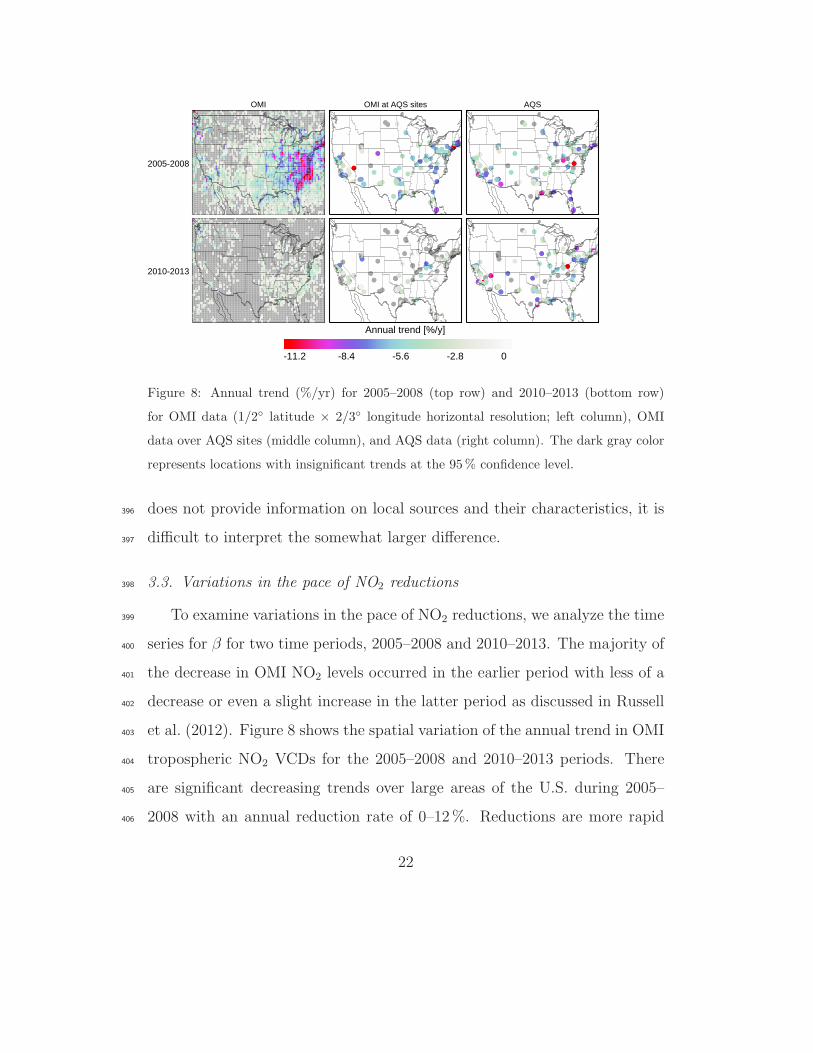
Figure 8: Annual trend (%/yr) for 2005–2008 (top row) and 2010–2013 (bottom row)

for OMI data (1/2 latitude × 2/3 longitude horizontal resolution; left column), OMI

data over AQS sites (middle column), and AQS data (right column). The dark gray color

represents locations with insignificant trends at the 95 % confidence level.

does not provide information on local sources and their characteristics, it is396

difficult to interpret the somewhat larger difference.397

3.3. Variations in the pace of NO2 reductions398

To examine variations in the pace of NO2 reductions, we analyze the time399

series for β for two time periods, 2005–2008 and 2010–2013. The majority of400

the decrease in OMI NO2 levels occurred in the earlier period with less of a401

decrease or even a slight increase in the latter period as discussed in Russell402

et al. (2012). Figure 8 shows the spatial variation of the annual trend in OMI403

tropospheric NO2 VCDs for the 2005–2008 and 2010–2013 periods. There404

are significant decreasing trends over large areas of the U.S. during 2005–405

2008 with an annual reduction rate of 0–12 %. Reductions are more rapid406

22

in many populated areas of the U.S.; trends in sparsely populated areas407

are small or insignificant. The trends are substantially weaker during 2010–408

2013. Figure 8 compares the trends observed by OMI and AQS monitors.409

The spatial distribution as well as the magnitude of the two trends for both410

periods are generally consistent, but are less so as compared to the entire411

2005–2013 period. OMI observations suggest a stronger average decrease of412

5 %/yr as compared to 3.7 %/yr from AQS data for 2005–2008, whereas the413

AQS data suggest a larger reduction of 2.8 %/yr as compared to 1.6 %/yr414

from OMI data for 2010–2013.415

There are two main reasons for the change in the pace of reductions.416

First, emission control devices (ECDs) were installed on many power plants417

by 2008, reducing their NOx emissions and, subsequently, the OMI NO2418

levels above the facilities dramatically (Duncan et al., 2013). The larger419

decrease seen in the eastern U.S. resulted from the 2005 Clean Air Interstate420

Rule (CAIR) for 27 eastern states with the goal to decrease NOx emissions421

from power plants. Second, U.S. emissions decreased in 2008 due to the422

global economic downturn. OMI NO2 levels changed little in many areas423

of the country in the latter period as the U.S. economy slowly recovered424

(Bishop and Stedman, 2014; Tong et al., 2014), but, at the same time, the425

fleet of light-duty vehicles continued to become more fuel efficient and less426

polluting (e.g. Bishop and Stedman, 2008; Russell et al., 2012) to meet the427

more stringent Tier 2 standards of the Clean Air Act Amendments of 1990.428

3.4. OMI NO2 trends over major U.S. metro areas and power plants429

In this section, we present the reductions in OMI NO2 VCDs for 20 U.S.430

metropolitan areas and over 150 of the largest U.S. power plants.431

23

2005-2008 2010-2013

-7.5-6.0-4.5-3.0-1.501.53.04.56.07.5

%/y

-3.7-3.0-2.2-1.5-0.700.71.52.23.03.7

x 1014 molec. cm-2/y

Figure 9: Relative (top) and absolute (bottom) annual trend in OMI tropospheric NO2

VCDs for 2005–2008 (left) and 2010–2013 (right) over 150 high-emitting U.S. power plants.

3.4.1. Trends over 20 metropolitan areas432

As shown in Figures 6 and 8, the largest percent decreases occurred in433

heavily populated, urban areas, which are collocated with the highest emis-434

sions. Table 4 shows the total reduction (%) in OMI NO2 levels for 20435

metropolitan areas for the period, 2005 to 2013, and the annual trends (%/yr)436

for the two sub-periods discussed in the previous section. Levels decreased437

by > 40 % in 8 of the 20 cities, including New York City, Los Angeles, and438

Philadelphia, 30–40 % in 6 cities, and 20–30 % in 6 cities. In all cities, the439

major decrease in levels occurred in the earlier period, 2005–2008, with small440

or insignificant changes in the latter period, 2010–2013.441

3.4.2. Trends over 150 power plants442

Over the OMI record, 2005–2013, U.S. NOx emissions from power plants443

decreased by about 52 % (http://www.epa.gov/ttn/chief/trends/index.444

24

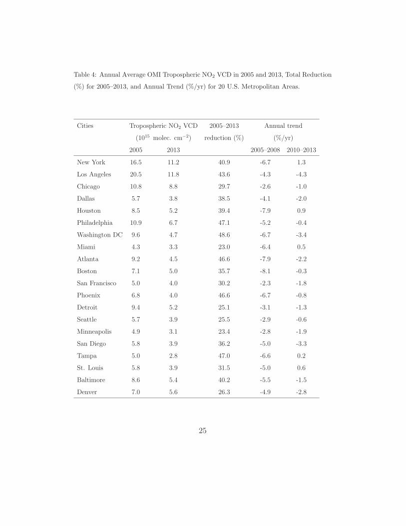
Table 4: Annual Average OMI Tropospheric NO2 VCD in 2005 and 2013, Total Reduction

(%) for 2005–2013, and Annual Trend (%/yr) for 20 U.S. Metropolitan Areas.

Cities Tropospheric NO2 VCD 2005–2013 Annual trend

(1015 molec. cm−2) reduction (%) (%/yr)

2005 2013 2005–2008 2010–2013

New York 16.5 11.2 40.9 -6.7 1.3

Los Angeles 20.5 11.8 43.6 -4.3 -4.3

Chicago 10.8 8.8 29.7 -2.6 -1.0

Dallas 5.7 3.8 38.5 -4.1 -2.0

Houston 8.5 5.2 39.4 -7.9 0.9

Philadelphia 10.9 6.7 47.1 -5.2 -0.4

Washington DC 9.6 4.7 48.6 -6.7 -3.4

Miami 4.3 3.3 23.0 -6.4 0.5

Atlanta 9.2 4.5 46.6 -7.9 -2.2

Boston 7.1 5.0 35.7 -8.1 -0.3

San Francisco 5.0 4.0 30.2 -2.3 -1.8

Phoenix 6.8 4.0 46.6 -6.7 -0.8

Detroit 9.4 5.2 25.1 -3.1 -1.3

Seattle 5.7 3.9 25.5 -2.9 -0.6

Minneapolis 4.9 3.1 23.4 -2.8 -1.9

San Diego 5.8 3.9 36.2 -5.0 -3.3

Tampa 5.0 2.8 47.0 -6.6 0.2

St. Louis 5.8 3.9 31.5 -5.0 0.6

Baltimore 8.6 5.4 40.2 -5.5 -1.5

Denver 7.0 5.6 26.3 -4.9 -2.8

25

html). Duncan et al. (2013) found that changes in OMI NO2 levels near445

55 power plants are consistent with changes in each facility′s emissions as446

reported to the CEMS and that the implementation of ECDs was clear in447

the OMI data for the majority of facilities. Figure 9 shows the annual change448

(%/yr) in OMI NO2 levels over 150 of the largest power plants in the U.S. The449

largest decreases occurred in the eastern U.S. and by 2008, which is consistent450

with compliance with the provisions of the CAIR. On average, OMI NO2451

levels decreased by 4.0 %/yr during the 2005–2008 period and by 0.6 %/yr452

during the 2010–2013 period. The number of power plants exhibiting positive453

trends increased from 10 during 2005–2008 to 59 during 2010–2013, although454

the trends are either small or insignificant (Figure 9).455

4. Discussion and conclusions456

Satellite data are currently being used in many air quality applications457

(e.g., Duncan et al., 2014) and uniquely have the advantage of spatial cover-458

age as compared to sparse surface networks. While the satellite data do not459

currently provide nose-level concentrations, they are of sufficient maturity460

that they do deliver important quantitative information on the trends and461

variations in pollutants important to the air quality community. For instance,462

Duncan et al. (2013) showed that trends and variations in OMI NO2 data463

above U.S. power plants agree well with trends and variations in their emis-464

sions reported to CEMS, particularly for large facilities. In this manuscript,465

we show the good correspondence of trends and variations in OMI NO2 VCD466

data to another common air quality quantity, surface concentration from the467

EPA AQS network of surface air quality monitors.468

26

Linear trends (2005–2013), estimated from OMI NO2 VCD data, com-469

pare well with those from AQS data when grouped by region, land use, and470

land type. We found that there are an insufficient number of surface NO2471

monitors (e.g., 0–2) in most cities to estimate an overall trend in a given472

metropolitan area. The under-representativeness of an individual monitor473

for a metropolitan region is highly dependent on site location, particularly474

those located near major pollution sources (e.g., highways). Nevertheless,475

the reductions (2005–2013) estimated from AQS data compare favorably for476

most metropolitan areas as discussed below.477

Several issues need to be considered when comparing trends and spatial478

and temporal variations estimated from OMI NO2 VCD data to those es-479

timated from surface data. The VCD data are influenced by NO2 levels in480

the free troposphere and the relatively coarse spatial resolution of the data481

may not allow for the VCD data to reflect the variations and trends near482

individual surface stations, particularly for those stations sited near major483

pollution sources. However, the satellite data provide greater spatial cov-484

erage as compared to the relative sparse monitoring network. In addition,485

AQS monitors measure species other than NO2, such as some fraction of NOz486

(= HNO3 + PAN + alkyl nitrates), where the NOz composition is typically487

unknown. Comparison of the trends inferred from collocated photolytic and488

molybdenum converter measurements suggests that the true NO2 trends are489

likely greater than those computed from AQS data.490

Despite the limitations of both satellite and surface data, they comple-491

ment each other and the correlation of the variations in the datasets is rela-492

tively high for some metropolitan areas. For example, Figure 10 shows the493

27

-1.0

-0.5

0.0

0.5

1.0r = 0.51, N = 6

-1.0-0.5

0.0

0.5

1.0

Chicago

-1.0

-0.5

0.0

0.5

1.0r = 0.49, N = 4

-1.0-0.5

0.0

0.5

1.0

Atlanta

-1.0

-0.5

0.0

0.5

1.0

A

QS

res

idua

l (R

)

r = 0.36, N = 10

-1.0-0.5

0.0

0.5

1.0

OM

I res

idua

l (R

)

Dallas

Year

-1.0

-0.5

0.0

0.5

1.0r = 0.43, N = 13

-1.0-0.5

0.0

0.5

1.0

Houston

2005 2006 2007 2008 2009 2010 2011 2012 2013

Figure 10: The normalized residual term, R, from Eq. 1 for four U.S. metropolitan areas.

The correlation coefficients (r) and number of AQS monitors (N) are given for each city.

The OMI data are sampled at the same locations as the AQS data.

normalized residual term, R, from Eq. 1. R reflects variations between the494

two datasets not explained by the seasonal cycle (α) nor the linear trend495

(β) regression terms. It incorporates fluctuations in NO2 associated with496

month-to-month variations in weather, but it also includes variations asso-497

ciated with the limitations of the two datasets (e.g., NOz interferents for498

AQS data). We will continue to work to understand the sources of some of499

the stronger deviations in R between the two datasets, such as those that500

occurred in late 2009 in both Houston and Dallas (Figure 10).501

In addition to understanding the sources of differences between the two502

datasets, work is ongoing to further refine and tailor the OMI NO2 retrieval503

28

Time of day

0

10

20

30

40

50

60

Ave

rage

red

uctio

n in

NO

2 [%]

AQSOMI

Rural Suburban Urban

1-2 3-4 5-6 7-8 9-10 11-12 13-14 15-16 17-18 19-20 21-22 23-24 LT

Figure 11: Diurnal changes in NO2 reductions calculated from 2-hour average NO2 mixing

ratios (circles) in rural (blue), suburban (green), and urban (orange) EPA AQS sites.

Dotted line represents average value for all land types. Values shown are the reductions

from 2005 to 2013. Diamonds represent reductions in OMI tropospheric NO2 VCDs. The

bars represent the 1σ variability of the average.

algorithm for air quality applications. In this manuscript, for instance, we504

showed that, by capturing the general trend in the vertical profile of NO2 con-505

centrations, the comparison between the satellite and surface data improves,506

particularly in less polluted areas. Our ongoing retrieval algorithm develop-507

ment consists of improved retrievals of SCDs (Marchenko et al., 2014), use508

of high-resolution MODIS surface reflectivity together with explicit aerosol509

corrections in the AMF calculation, and coupled NO2 and cloud retrievals,510

and these improvements should improve the quality of OMI NO2 data and511

their scientific applications.512

As a final comment, the Aura satellite overpasses a given location once513

a day in early afternoon local time, which limits the data′s usefulness, such514

as for estimating the diurnal variation of emissions from mobile and point515

29

sources. Concentrations of NO2 in urban areas undergo strong diurnal vari-516

ations with higher values during the night when photolysis ceases to convert517

NO2 to NO, a trace gas that is a member of the NOx family that cannot518

be measured from space, and the boundary layer height shrinks, trapping519

fresh NOx emissions near the surface, particularly in early morning during520

rushhour. For our purpose of estimating NO2 trends, we found that there is521

little variation in the reductions estimated from AQS data during daylight522

hours and the reductions estimated from OMI data. Figure 11 indicates523

that the reductions during the night are generally lower than during the day524

(i.e., 27 % at 5–6 AM to 38 % at 3–4 PM), which should be considered when525

inferring changes in emissions, such as mobile sources, from the OMI data.526

There are two upcoming satellite missions that are relevant for air quality527

applications using NO2 VCD data, including the application presented in this528

manuscript. Both instruments will provide data similar to the OMI, but with529

improved capabilities. The NASA Tropospheric Emissions: Monitoring of530

Pollution (TEMPO) instrument (Chance et al., 2013) will be in geostationary531

orbit, continuously observing the U.S. during daylight hours; the satellite′s532

orbital period will match the Earth′s rotational period, so the satellite will533

appear to be motionless to an observer on the Earth′s surface. This orbit will534

improve the signal-to-noise ratio of the data and allow for the estimation of535

NO2 trends and emissions throughout the day. The European Space Agency′s536

(ESA) Tropospheric Ozone Monitoring Instrument (TROPOMI, (Veefkind537

et al., 2012)) will be launched in 2016 and have a similar once daily overpass538

time as OMI, but its pixels will have finer spatial resolution, which will539

allow for better detection of smaller emissions sources and likely improve the540

30

comparison of trends and variations with AQS data.541

AppendixA. Graphical illustration of the multivariate regression542

analysis543

Figure A1 illustrates the variation of the four subcomponents with time544

from OMI tropospheric NO2 columns over the eastern U.S. In this example,545

seasonal variation and linear trend contribute, respectively, 74 % and 11 % of546

the total variance. The residual contains the impact of short-term variations547

(e.g. transport) in NO2 columns that were not captured by the regression548

model, and represents about 12 % of the total variance. The original and549

modeled time series constructed from seasonal and trend components are550

highly correlated (r = 0.92, N = 108), suggesting that the approach offers a551

simple yet robust seasonal and trend estimates.552

AppendixB. The GMI model553

The GMI CTM is driven by meteorology from the Modern Era Retrospective-554

Analysis for Research and Applications (MERRA) (Rienecker et al., 2011),555

which reasonably reproduces observed weather for the Aura record (2005–556

2013). The simulation is performed at 1 latitude × 1.25 longitude horizon-557

tal resolution and with 72 vertical levels extending from the surface to 0.01558

hPa. About 33 levels are in the troposphere, including 8 levels below 1 km.559

The model output is sampled at the OMI overpass time for a self-consistent560

comparison with the observational dataset.561

We use a simulation for 2005–2010 that uses monthly and annually vary-562

ing emissions of CO, NOx, and non-methane hydrocarbons. Anthropogenic563

31

012345

Obs

erva

tions data

fitted curve

012345

Sea

sona

l ter

m α1

-1.0-0.5

0.0

0.5

1.0

Cha

nges

in

sea

sona

l am

plitu

de

α2

-1.0

-0.5

0.0

0.5

Tre

nd

β

Year

-2-1

0

1

2

Res

idua

l R

2005 2006 2007 2008 2009 2010 2011 2012 2013

Figure A1: Time series of monthly OMI tropospheric NO2 columns (Ω, 1015 molecules

cm−2) over the eastern U.S. (36–40N, 70–75W) separated into four subcomponents:

seasonal cycle and change in seasonal amplitude (α = α1 + α2), long-term linear trend

(β), and residuals (R). The line in the top row represents the summation of the α and β

subcomponents, and the filled circles represent the actual OMI data.

32

emissions are based on the EDGAR3.2 Inventory (Olivier et al., 2005), over-564

written by regional inventories: The EPA NEI 2005 inventory (http://www.565

epa.gov/ttnchie1/net/2005inventory.html) over the U.S., CAC (https:566

//www.ec.gc.ca) over Canada, BRAVO over Mexico (Kuhns et al., 2005),567

the European Monitoring and Evaluation Programme (EMEP, http://www.568

emep.int) over Europe, and inventory from Zhang et al. (2009) over Asia.569

The anthropogenic emissions prior to 2006 are scaled applying annual scaling570

factors from the GEOS-Chem model (van Donkelaar et al., 2008). For 2007–571

2010, the U.S. and European emissions are scaled on a country-wide basis572

using the national emission totals from EPA and EMEP, respectively. The573

REAS inventory projections (Ohara et al., 2007) are used to scale the Asian574

anthropogenic emissions for 2007–2009. Soil NOx emissions are computed575

online with temperature and precipitation dependence ((Yienger and Levy,576

1995). Lightning NOx emissions are calculated following Allen et al. (2010).577

AppendixC. Details of the OMI retrieval algorithm578

We use the OMI standard product, OMNO2 (version 2.1), which is pub-579

licly available from the NASA Goddard Earth Sciences Data Active Archive580

Center (GES DISC, http://disc.sci.gsfc.nasa.gov). This data version581

includes significant updates and improvements over previous versions (Buc-582

sela et al., 2006; Celarier et al., 2008; Lamsal et al., 2008, 2010). Detailed583

descriptions of the current algorithm and assessments for the standard OMI584

NO2 product are given in Bucsela et al. (2013) and Lamsal et al. (2014),585

respectively. In brief, the algorithm retrieves NO2 slant column densities586

(SCDs) with the Differential Optical Absorption Spectroscopy (DOAS) tech-587

33

nique (Platt, 1994) in the visible region (405–465 nm). This is followed by588

computation of air mass factors (AMFs) by integrating relative vertical dis-589

tribution (shape factors) of NO2 weighted by altitude dependent scattering590

weight factors. The NO2 vertical profiles are simulated by the GMI CTM591

(Strahan et al., 2007; Duncan et al., 2007) at 2 latitude × 2.5 longitude hor-592

izontal resolution for the time of the OMI measurement. Scattering weights593

are computed as a function of reflectivity and pressure of cloud and terrain,594

and viewing geometry with a radiative transfer model. Stratospheric AMFs595

and retrieved SCDs from five consecutive orbits over clean regions (30S–5N)596

are used to correct for cross-track biases (stripes) in SCDs resulting from cal-597

ibration errors. Stratospheric NO2 fields needed to derive tropospheric NO2598

VCDs are determined by box-car smoothing and interpolation of OMI NO2599

VCDs estimates, after accounting for a priori tropospheric NO2 VCDs over600

unpolluted or cloudy areas. Comparison of OMI tropospheric NO2 VCDs601

with a suite of in situ and remote sensing measurements suggests agreement602

within ± 20 % for clear-sky conditions (Lamsal et al., 2014).603

Acknowledgements604

The work was supported by the NASA Air Quality Applied Science Team605

(AQAST) and NASA′s Earth Science Directorate Atmospheric Composition606

Programs.607

References608

Allen, D., Pickering, K., Duncan, B., Damon, M., 2010. Impact of light-609

ning no emissions on north american photochemistry as determined us-610

34

ing the global modeling initiative (gmi) model. J. Geophys. Res. 115,611

doi:10.1029/2010jd014062.612

Beirle, S., Platt, U., Wenig, M., Wagner, T., 2003. Weekly cycle of NO2613

by GOME measurements: a signature of anthropogenic sources. Atmos.614

Chem. Phys. 3, 2225–2232.615

Bishop, G. A., Stedman, D. H., 2008. A decade of on-road emissions mea-616

surements. Environ. Sci. Technol. 42, 1651–1656, DOI: 10.1021/es702413b.617

Bishop, G. A., Stedman, D. H., 2014. The recession of 2008 and its impact on618

light-duty vehicle emissions in three western United States cities. Environ.619

Sci. Technol. 48, 14822–14827, DOI: 10.1021/es5043518.620

Boersma, K. F., Eskes, H. J., Brinksma, E. J., 2004. Error analy-621

sis for tropospheric NO2 retrieval from space. J. Geophys. Res. 109,622

doi:10.1029/2003JD003962.623

Boersma, K. F., Eskes, H. J., Dirksen, R. J., van der A, R. J., Veefkind,624

J. P., et al., 2011. An improved tropospheric no2 column retrieval algorithm625

for the ozone monitoring instrument. Atmos. Meas. Tech. 4, 1905–1928,626

doi:10.5194/amt-4-1905-2011.627

Boersma, K. F., Jacob, D. J., Bucsela, E. J., Perring, A. E., Dirksen, R., van628

der A, R. J., Yontosca, R. M., Park, R. J., Wenig, M. O., Bertram, T. H.,629

Cohen, R. C., 2008a. Validation of OMI tropospheric NO2 observations630

during INTEX-B and application to constrain NOx emissions over the631

eastern United States and Mexico. Atmos. Environ. 42, 4480–4497.632

35

Boersma, K. F., Jacob, D. J., Eskes, H. J., Pinder, R. W., Wang, J., van der633

A, R. J., 2008b. Intercomparison of SCIAMACHY and OMI tropospheric634

NO2 columns: observing the diurnal evolution of chemistry and emissions635

from space. J. Geophys. Res. 113, doi:10.1029/2007JD008816.636

Bucsela, E. J., Celarier, E. A., Wenig, M. O., Gleason, J. F., Veefkind, J. P.,637

Boersma, K. F., Brinksma, E. J., 2006. Algorithm for NO2 vertical column638

retrieval from the Ozone Monitoring Instrument. IEEE Trans. Geo. Rem.639

Sens. 44, 1245–1258.640

Bucsela, E. J., Krotkov, N. A., Celarier, E. A., Lamsal, L. N., Swartz, W. H.,641

Bhartia, P. K., Boersma, K. F., Veefkind, J. P., Gleason, J. F., Pickering,642

K. E., 2013. A new stratospheric and tropospheric NO2 retrieval algorithm643

for nadir-viewing satellite instruments: application to OMI. Atmos. Meas.644

Tech. 6, 2607–2626.645

Castellanos, P., Boersma, K. F., 2012. Reductions in nitrogen oxides over646

Europe driven by environmental policy and economic recession. Sci. Rep.647

2, 2, 265, DOI:10.1038/srep00265.648

Celarier, E. A., Brinksma, E. J., Gleason, J. F., Veefkind, J. P., Cede, A.,649

Herman, J. R., Ionov, D., Goutail, F., Pommereau, J. P., Lambert, J. C.,650

van Roozendael, M., Pinardi, G., Witrrock, F., Schonhardt, A., Richter,651

A., Ibrahim, O. W., Wagner, T., Bojkov, B., Mount, G., Spinei, E., Chen,652

C. M., Pongetti, T. J., Sander, S. P., Bucsela, E. J., Wenig, M. O., Swart,653

D. P. J., Volten, H., Kroon, M., Levelt, P. F., 2008. Validation of Ozone654

Monitoring Instrument nitrogen dioxide columns. J. Geophys. Res. 113,655

doi:10.1029/2007JD008908.656

36

Challen, P., Hickish, D., Bedford, J., 1958. An investigation of some health657

hazards in an inert-gas tungsten-arc welding shop. Br. J. Ind. Med. 15,658

276–282.659

Chance, K., Liu, X., Suleiman, R. M., Flittner, D. E., Al-Saadi, J., Janz,660

S. J., 2013. Tropospheric emissions: Monitoring of pollution (TEMPO).661

SPIE Publication, 8866–11.662

Cleveland, R. B., Cleveland, W. S., McRae, J. E., Terpenning, I., 1990. STL:663

A seasonal-trend decomposition procedure based on Loess. J. Off. Stat. 6,664

1, 3–33.665

Demerjian, K. L., 2000. A review of national monitoring networks in North666

America. Atmos. Environ. 34, 1861–1884.667

Duncan, B. N., Chameides, W., 1998. The effects of urban emission control668

strategies on the export of ozone and ozone precursors from the urban669

atmosphere to the troposphere. J. Geophys. Res. 103, 28,159–28179.670

Duncan, B. N., Prados, A. I., Lamsal, L. N., Liu, Y., Streets, D., Gupta,671

P., Hilsenrath, E., Kahn, R., Nielsen, J. E., Beyersdorf, A., Burton, S.,672

Fiore, A. M., Fishman, J., Henze, D., Hostetler, C., Krotkov, N. A., Lee,673

P., Lin, M., Pawson, S., Pfister, G., Pickering, K. E., Pierce, B., Yoshida,674

Y., Ziemba, L., 2014. Satellite data of atmospheric pollution for U.S. air675

quality applications: Examples of applications, summary of data end-user676

resources, answers to FAQs, and common mistakes to avoid. Atmos. Env-677

iron. 94.678

37

Duncan, B. N., Strahan, S. E., Yoshida, Y., Steenrod, S. D., Livesey, N.,679

2007. Model study of the cross-tropopause transport of biomass burning680

pollution. Atmos. Chem. Phys. 7, 3713–3736.681

Duncan, B. N., Yoshida, Y., de Foy, B., Lamsal, L. N., Streets, D., Lu, Z.,682

Pickering, K. E., Krotkov, N. A., 2013. The observed response of the Ozone683

Monitoring Instrument (OMI) NO2 column to NOx emission controls on684

power plants in the United States: 2005-2011. Atmos. Environ. 81, 102–685

111.686

Duncan, B. N., Yoshida, Y., Olson, J., Sillman, S., Martin, R. V., Lamsal,687

L. N., Hu, Y., Pickering, K., Retscher, C., Allen, D., Crawford, J., 2010.688

Application of OMI observations to a space-based indicator of NOx and689

VOC controls on surface ozone formation. Atmos. Environ. 44, 2213–2223.690

Dunlea, E. J., Herndon, S. C., Nelson, D. D., Volkamer, R. M., San Martini,691

F., Sheehy, P. M., Zahniser, M. S., Shorter, J. H., Wormhoudt, J., Lamb,692

B. K., Allwine, E. J., Gaffney, J. S., Marley, N. A., Grutter, M., Marquez,693

C., Blanco, S., Cardenas, B., Retama, A., Ramos Villegas, C. R., Kolb,694

C. E., Molina, L. T., Molina, M. J., 2007. Evaluation of nitrogen diox-695

ide chemiluminescence monitors in a polluted urban environment. Atmos.696

Chem. Phys. 7, 2691–2704.697

Edgerton, E. S., Hartsell, B. E., Saylor, R. D., Jansen, J. J., Hansen, D. A.,698

Hidy, G. M., 2006. The Southeastern Aerosol Research and Characteriza-699

tion Study, part 3: Continuous measurements of fine particulate matter700

mass and composition. J. Air Waste Mgt. Assoc. 56(9), 1325–1341.701

38

EPA, 1975. Technical assistance document for the chemiluminescence mea-702

surement of nitrogen dioxide, tech. rep.,. Tech. rep., U.S. Environmental703

Protection Agency, Research Triangle Park, NC 27711, EPA-600/4-75-003.704

EPA, 2006. Air quality criteria for ozone and related photochemical oxi-705

dants. Tech. rep., U.S. Environmental Protection Agency, Research Trian-706

gle Park,NC 27711, EPA 454/K-01-002.707

EPA, 2008. Integrated science assessment for oxides of nitrogen - health crite-708

ria (first external review draft). Tech. rep., U.S. Environmental Protection709

Agency, Research Triangle Park,NC 27711, EPA/600/R-07/093.710

EPA, 2012. Our nation’s air: Status and trends through 2010. Tech. rep.,711

Environmental Protection Agency, EPA-454/R-12001.712

Frost, G. J., McKeen, S. A., Trainer, M., Ryerson, T. B., Neuman, J. A.,713

Roberts, J. M., Swanson, A., Holloway, J. S., Sueper, D. T., Fortin, T.,714

Parrish, D. D., Fehsenfeld, F., Flocke, F., Peckham, S. E., Grell, G. A.,715

Kowal, D., Cartwright, J., Auerbach, N., Habermann, T., 2006. Effects of716

changing power plant NOx emissions on ozone in the eastern United States:717

Proof of concept. J. Geophys. Res. 111, doi:10.1029/2005JD006354.718

Ghude, S. D., Pfister, G. G., Jena, C., et al., 2013. Satellite constraints of719

nitrogen oxide emissions from India based on OMI observations and WRF-720

Chem simulations. Geophys. Res. Lett. 40, doi:10.1029/2012GL053926.721

Grosjean, D., Harrison, J., 1985. Response of chemiluminescence NOx ana-722

lyzers and ultraviolet ozone analyzers to organic air pollutants. Environ.723

Sci. Technol. 19, 862–865.724

39

Hains, J., Boersma, K. F., Kroon, M., et al., 2010. Testing and improving725

OMI DOMINO tropospheric NO2 using observations from the DANDE-726

LIONS and INTEX-B validation campaigns. J. Geophys. Res. 115, D05301,727

doi:10.1029/2009JD012399.728

Heckel, A., Kim, S. W., Frost, G. J., Richter, A., Trainer, M., Burrows, J. P.,729

2011. Influence of low spatial resolution a priori data on tropospheric NO2730

satellite retrievals. Atmos. Meas. Tech. 4(9), 1805–1820, doi:10.5194/amt-731

4-1805-2011.732

Hilboll, A., Richter, A., Burrows, J. P., 2013. Long-term changes of tropo-733

spheric NO2 over megacities derived from multiple satellite instruments.734

Atmos. Chem. Phys. 13, 4145–4169, doi:10.5194/acp-13-4145-2013.735

Jaegle, L., Steinberger, L., Martin, R. V., Chance, K., 2005. Global parti-736

tioning of NOx sources using satellite observations: Relative roles of fossil737

fuel combustion, biomass burning and soil emissions. Faraday Discussions738

130, doi: 10.1039/b502128f.739

Kim, S. W., Heckel, A., McKeen, S. A., Frost, G. J., Hsie, E. Y.,740

Trainer, M. K., Richter, A., Burrows, J. P., Peckham, S. E., Grell,741

G. A., 2006. Satellite-observed U.S. power plant NOx emission reduc-742

tions and their impact on air quality. Geophys. Res. Lett. 33, L22812,743

doi:10.1029/2006GL027749.744

Kleinfield, M., Giel, C., Tabershaw, I., 1957. Health hazards associated with745

inert gas shield metal arc welding. Arch. Ind. Health 15, 27–31.746

40

Kley, D., McFarland, M., 1980. Chemiluminescence detector for NO and747

NO2. Atmos. Tech. 12, 63–69.748

Kuhns, H., Knipping, E. M., Vokovich, J. M., 2005. Development of a United749

States-Mexico emissions inventory for the Big Bend Regional Aerosol and750

Visibility Observational (BRAVO) study. J. Air Waste Mgt. Assoc. 55,751

677–692.752

Lamsal, L. N., Krotkov, N. A., Celarier, E. A., Swartz, W. H., Pickering,753

K. E., Bucsela, E. J., Gleason, J. F., Martin, R. V., Philip, S., Irie, H.,754

Cede, A., Herman, J., Weinheimer, A., Szykman, J. J., Knepp, T. N., 2014.755

Evaluation of OMI operational standard no2 column retrievals using in situ756

and surface-based no2 observations. Atmos. Chem. Phys. 14, 11587-11609,757

doi:10.5194/acp-14-11587-2014.758

Lamsal, L. N., Martin, R. V., Padmanabhan, A., van Donkelaar, A., Zhang,759

Q., Sioris, C. E., Chance, K., Kurosu, T. P., Newchurch, M. J., 2011.760

Application of satellite observations for timely updates to global an-761

thropogenic NOx emission inventories. Geophys. Res. Lett. 38, L05810,762

doi:10.1029/2010GL046476.763

Lamsal, L. N., Martin, R. V., van Donkelaar, A., Celarier, E. A., Bucsela,764

E. J., Boersma, K. F., Luo, R. D. C., Wang, Y., 2010. Indirect validation765

of tropospheric nitrogen dioxide retrieved from the OMI satellite instru-766

ment: Insight into the seasonal variation of nitrogen oxides at northern767

midlatitudes. J. Geophys. Res. 115, D05302, doi:10.1029/2009JD013351.768

Lamsal, L. N., Martin, R. V., van Donkelaar, A., Steinbacher, M., Celarier,769

41

E. A., Bucsela, E., Dunlea, E. J., Pinto, J. P., 2008. Ground-level nitrogen770

dioxide concentrations inferred from the satellite-borne Ozone Monitoring771

Instrument. J. Geophys. Res. 113, D16308, doi:10.1029/2007JD009235.772

Leue, C., Wenig, M., Wagner, T., Klimm, O., Platt, U., Jahne, B., 2001.773

Quantitative analysis of NO2 emissions from Global Ozone Monitoring774

Experiment satellite image sequences. J. Geophys. Res. 106, 5493–5505.775

Lin, J. T., McElroy, M. B., 2011. Detection from space of a reduction in776

anthropogenic emissions of nitrogen oxides during the Chinese economic777

downturn. Atmos. Chem. Phys. 11, 8171–8188, doi:10.5194/acp-11-8171-778

2011.779

Lin, J. T., McElroy, M. B., Boersma, K. F., 2010. Constraint of anthro-780

pogenic NOx emissions in China from different sectors: a new methodology781

using multiple satellite retrievals. Atmos. Chem. Phys. 10, 63–78.782

Marchenko, S., Krotkov, N. A., Lamsal, L. N., Celarier, E. A., Swartz, W. H.,783

Bucsela, E. J., 2014. Towards a more accurate slant column density re-784

trieval of nitrogen dioxide from space. J. Geophys. Res. TBD, submitted.785

Martin, R. V., Chance, K., Jacob, D. J., et al., 2002. An improved re-786

trieval of tropospheric nitrogen dioxide from GOME. J. Geophys. Res.787

107, doi:10.1029/2001JD001027.788

Martin, R. V., Jacob, D. J., Chance, K., Kurosu, T. P., Perner, P. I.,789

Evans, M. J., 2003. Global inventory of nitrogen oxide emission con-790

strained by space-based observations of NO2 columns. J. Geophys. Res.791

108, doi:10.1029/2003JD003453.792

42

Martin, R. V., Parrish, D. D., Ryerson, T. B., Jr., D. K. N., Chance, K.,793

Kurosu, T. P., Jacob, D. J., Sturges, E. D., Fried, A., Wert, B. P., 2004.794

Evaluation of GOME satellite measurements of tropospheric NO2 and795

HCHO using regional data from aircraft campaigns in the southeastern796

United States. J. Geophys. Res. 109, doi:10.1029/2004JD004869.797

McDonald, B. C., Dallmann, T. R., Martin, E. W., Harley, R. A., 2012.798

Long-term trends in nitrogen oxide emissions from motor vehicles at799

national, state, and air basin scales. J. Geophys. Res. 117, D00V18,800

doi:10.1029/2012JD018304.801

Napelenok, S. L., Pinder, R. W., Gilliland, A. B., Martin, R. V., 2008. A802

method for evaluating spatially-resolved NOx emissions using Kalman filter803

inversion, direct sensitivities, and space-based NO2 observations. Atmos.804

Chem. Phys. 8, 5603–5614.805

Ohara, T., Akimoto, H., Kurokawa, J., Horii, N., Yamaji, K., Yan, X.,806

Hayasaka, T., 2007. An Asian emission inventory of anthropogenic emis-807

sion sources for the period 1980–2020. Atmos. Chem. Phys. 7, 4419–4444.808

Olivier, J. G., Van Aardenne, J. A., Dentener, F. J., Pagliari, V., Ganzeveld,809

L. N., Peters, J. A., 2005. Recent trends in global greenhouse gas emissions:810

regional trends 19702000 and spatial distributionof key sources in 2000.811

Environ. Sci. 2(2-3), 81–99.812

Platt, U., 1994. Differential Optical Absorption Spectroscopy (DOAS). In:813

Sigrist, M. W. (Ed.), Air Monitoring by Spectroscopic Techniques. John814

Wiley, New York, USA, pp. 27–84.815

43

Pollack, I. B., Lerner, B. M., Ryerson, T. B., 2010. Evaluation of ultravio-816

let light-emitting diodes for detection of atmospheric NO2 by photolysis817

chemiluminescence. J. Atmos. Chem. 65, 111–125.818

Randel, W. J., Cobb, J. B., 1994. Coherent variations of monthly mean total819

ozone and lower stratospheric temperature. J. Geophys. Res. 99, 5433–820

5447, doi:10.1029/93JD03454.821

Richter, A., Burrows, J. P., Nuß, H., Granier, C., Niemeier, U., 2005. Increase822

in tropospheric nitrogen dioxide levels over China observed from space.823

Nature 437, 129–132.824

Rienecker, M. M., Suarez, M. J., Gelaro, R., Todling, R., Bacmeister, J.,825

Liu, E., Bosilovich, M. G., Schubert, S. D., Takacs, L., Kim, G. K.,826

Bloom, S., Chen, J., Collins, D., Conaty, A., da Silva, A., Gu, W.,827

Joiner, J., Koster, R. D., Lucchesi, R., Molod, A., Owens, T., Pawson,828

S., Pegion, P., Redder, C. R., Reichle, R., Robertson, F. R., Ruddick,829

A. G., Sienkiewicz, M., Woollen, J., 2011. MERRA: NASAs Modern-Era830

Retrospective Analysis for Research and Applications. J. Clim. 24, doi:831

http://dx.doi.org/10.1175/JCLI-D-11-00015.1.832

Russell, A. R., Perring, A. E., Valin, L. C., Hudman, R. C., Browne, E. C.,833

Min, K. E., Wooldridge, P. J., Cohen, R. C., 2011. A high spatial resolu-834

tion retrieval of NO2 column densities from OMI: method and evaluation.835

Atmos. Chem. Phys. 11, 8543–8554, doi:10.5194/acp-11-8543-2011.836

Russell, A. R., Valin, L. C., Cohen, R. C., 2012. Trends in OMI NO2 ob-837

servations over the United States: effects of emission control technol-838

44

ogy and the economic recession. Atmos. Chem. Phys. 12, 12197–12209,839

doi:10.5194/acp-12-12197-2012.840

Ryerson, T. B., Williams, E. J., Fehsenfeld, F. C., 2000. An efficient pho-841

tolysis system for fast-response NO2 measurements. J. Geophys. Res. 105,842

26447–26461.843

Steinbacher, M., Zellweger, C., Schwarzenbach, B., Bugmann, S., Buchmann,844

B., Ordonez, C., Prevot, A. S. H., Hueglin, C., 2007. Nitrogen oxides mea-845

surements at rural sites in Switzerland: Bias of conventional measurement846

techniques. J. Geophys. Res.10.1029/2006JD007971.847

Strahan, S. E., Duncan, B. N., Hoor, P., 2007. Observationally derived trans-848

port diagnostics for the lowermost stratosphere and their application to the849

GMI chemistry and transport model. Atmos. Chem. Phys. 7, 2435–2445.850

Streets, D. G., Carmichael, G. R., de Foy, B., Dickerson, R. R., Duncan,851

B. N., Edwards, D. P., Haynes, J. A., Henze, D. K., Houyoux, M. R.,852

Jacob, D. J., Krotkov, N. A., Lamsal, L. N., Liu, Y., Lu, Z., Martin, R. V.,853

Pfister, G. G., Pinder, R. W., Wecht, K. J., 2013. Emissions estimation854

from satellite retrievals: A review of current capability. Atmos. Environ.855

77, 1011–1042.856

Strode, S. A., Rodriguez, J. M., Logan, J. A., Cooper, O. R., Witte,857

J. C., Lamsal, L. N., Damon, M., Steenrod, S. D., Strahan, S. E., 2014.858

Trends and variability in surface ozone over the United States. J. Geophys.859

Res.Submitted.860

45

Tang, W., Cohan, D., Lamsal, L. N., Xiao, X., Zhou, W., 2013. Inverse861

modeling of Texas NOx emissions using space-based and ground-based NO2862

observations. Atmos. Chem. Phys. 13, 11005–11018.863

Tang, W., Cohan, D., Pour-Biazar, A., Lamsal, L. N., White, A., Xiao, X.,864

Zhou, W., Henderson, B. H., Lash, B., 2014. Influence of satellite-derived865

photolysis rates and NOx emissions on Texas ozone modeling. Atmos.866

Chem. Phys. Discuss. 7, 11415–11437, doi:10.5194/acpd-14-24475-2014.867

Tong, D., Lamsal, L. N., Pan, L., Kim, H., Lee, P., Chai, T., Pickering,868

K. E., 2014. Long-term NOx trends over large cities in the United States:869

Intercomparison of satellite retrievals, ground observations, and emission870

inventories. Atmos. Environ. TBD, submitted.871

Valin, L. C., Russell, A. R., Cohen, R. C., 2013. Variation of OH radical in872

an urban plume inferred from NO2 column measurements. Geophys. Res.873

Lett. 40, 1856–1860.874

van Donkelaar, A., Martin, R. V., Leaitch, W. R., Macdonald, A. M., Walker,875

T. W., Streets, D. G., Zhang, Q., Dunlea, E. J., Jimenez, J. L., Dibb,876

J. E., Huey, L. G., Weber, R., Andreae, M. O., 2008. Analysis of aircraft877

and satellite measurements from the Intercontinental Chemical Transport878

Experiment (INTEX-B) to quantify long-range transport of East Asian879

sulfur to Canada. Atmos. Chem. Phys. 8, 2999–3014.880

Veefkind, J. P., Aben, I., McMullan, K., Foerster, H., de Vries, J., Otter,881

G., Claas, J., Eskes, H. J., de Haan, J. F., Kleipool, Q., van Weele, M.,882

Hasekamp, O., Hoogeveen, R., Landgraf, J., Snel, R., Tol, P., Ingmann,883

46

P., Voors, R., Kruizinga, B., Vink, R., Visser, H., Levelt, P. F., 2012.884

TROPOMI on the ESA Sentinel-5 Precursor: A GMES mission for global885

observations of the atmospheric composition for climate, air quality and886

ozone layer applications. Rem. Sen. Env. 120, 70–83.887

Vinken, G. C. M., Boersma, K. F., van Donkelaar, A., Zhang, L., 2014.888

Constraints on ship NOx emissions in Europe using GEOS-Chem and889

OMI satellite NO2 observations. Atmos. Chem. Phys. 14, 1353–1369,890

doi:10.5194/acp-14-1353-2014.891

Wang, S. W., Zhang, Q., Streets, D. G., He, K. B., Martin, R. V., Lamsal,892

L. N., Chen, D., Lei, Y., Lu, Z., 2012. Growth in NOx emissions from893

power plants in China: bottom-up estimates and satellite observations.894

Atmos. Chem. Phys. 12, 4429–4447, doi:10.5194/acp-12-4429-2012.895

Wang, Y. X., McElroy, M. B., Martin, R. V., Streets, D. G., Zhang, Q.,896

Fu, T.-M., 2007. Seasonal variability of NOx emissions over east China897

constrained by satellite observations: Implications for combustion and mi-898

crobial sources. J. Geophys. Res. 112, doi:10.1029/2006JD007538.899

Winer, A. M., Peters, J. W., Smith, J. P., Pitts Jr., J. N., 1974. Response900

of commercial chemiluminescent NO-NO2 analyzers to other nitrogen con-901

taining compounds. Environ. Sci. Technol. 8, 1118–1121.902

Xing, J., Pleim, J., Mathur, R., Pouliot, G., Hogrefe, C., Gan, C. M., Wei, C.,903

2013. Historical gaseous and primary aerosol emissions in the United States904

from 1990 to 2010. Atmos. Chem. Phys. 13, 7531–7549, doi:10.5194/acp-905

13-7531-2013.906

47

Yienger, J. J., Levy, H., 1995. Empirical model of global soil biogenic NOx907

emissions. J. Geophys. Res. 100, 11447–11464.908

Zellweger, C., Ammann, M., Buchmann, B., Hofer, P., Lugauer, M., Rutti-909

mann, R., Streit, N., Weingartner, E., Baltensperger, U., 2000. Summer-910

time NOy speciation at the Jungfraujoch, 3580 m above sea level, Switzer-911

land. J. Geophys. Res. 105, 6655–6667.912

Zhang, Q., Streets, D. G., Carmichael, G. R., He, K., Huo, H., Kannari, A.,913

Klimont, Z., Park, I., Reddy, S., Fu, J. S., Chen, D., Duan, L., Lei, Y.,914

Wang, L., Yao, Z., 2009. Asian emissions in 2006 for the NASA INTEX-B915

mission. Atmos. Chem. Phys. Discuss. 9, 4081–4139.916

Zhao, C., Wang, Y., 2009. Assimilation inversion of NO2 emissions over917

east Asia using OMI NO2 column measurements. Geophys. Res. Lett. 36,918

L06805, doi:10.1029/2008GL037129.919

Zhou, Y., Brunner, D., Hueglin, C., s. Henne, Staehelin, J., 2012. Changes920

in OMI tropospheric NO2 columns over Europe from 2004 to 2009 the921

influence of meteorological variability. Atmos. Environ. 46.922

48