us mexico cooperation on reducing emissions from ships through

U.S.-Mexico Cooperation on Reducing Emissions from Ships through a Mexican Emission Control Area: Development of the First National Mexican Emission

Inventories for Ships Using the Waterway Network Ship Traffic, Energy, and Environmental

Model (STEEM)

United States

Environmental Protection

Agency

Office of International and Tribal Affairs

EPA-160-R-15-001

May 2015

Disclaimer

This technical report does not necessarily represent final EPA decisions or positions. It is intended to present technical analysis of issues using data that are currently available and were collected through this project. The purpose in the release of such reports is to facilitate the exchange of technical information and to inform the public of technical developments which may form the basis for policy action by EPA or other entities.

Prepared under EPA Contract EP-W-09-024

Contributors to this report are Angela Bandemehr and Brian Muehling of the U.S. Environmental Protection Agency, Jim Corbett and Bryan Comer of Energy and Environmental Research Associates, and Jeanine Boyle of the Battelle Memorial Institute.

For more information please contact: Angela Bandemehr Office of International and Tribal Affairs U.S. Environmental Protection Agency 202.564.1427 [email protected]

EPA-160-R-15-001 | May 2015 i

Table of Contents

Abbreviations and Acronyms ........................................................................................................................ iii

Executive Summary ..................................................................................................................................... iv

1.0 Introduction ........................................................................................................................................ 1

1.1 History of the Development of a Mexican Emission Control Area ......................................... 1

1.2 Requirements for Establishing an Emission Control Area ..................................................... 2

1.3 Assessing the Impact of an ECA on Ship Emissions in Mexico............................................. 3

2.0 Methodology ...................................................................................................................................... 3

2.1 Overview of the Emissions Inventory Modeling Process ....................................................... 4

2.2 STEEM ................................................................................................................................... 6

2.3 Estimating 2013 Ship Emissions ............................................................................................ 7

2.4 Estimating 2030 Ship Emissions ............................................................................................ 9

2.5 Port Emissions ..................................................................................................................... 10

3.0 Results ............................................................................................................................................ 11

4.0 Conclusions ..................................................................................................................................... 12

5.0 Reference ........................................................................................................................................ 13

Appendices

APPENDIX I: Key MARPOL Annex VI Standards (Global and ECA)

APPENDIX II: Required Elements of an ECA Designation Proposal

APPENDIX III: 2011 Ship Emission Inventory Results

List of Figures

Figure 1. Progression of steps needed to support an ECA designation (adapted from SEMARNAT, 2013). ......................................................................................................................................................... 2

Figure 2. STEEM total modeling domain (inset box outlined in blue) and potential Mexican ECA (dark green shaded area). The portion of the North American ECA near Mexico (light green shaded area) is also shown. ......................................................................................................................... 4

Figure 3. STEEM network representation, including ~1700 World Ports. STEEM estimates emissions from nearly complete historical North American shipping activities and individual ship attributes. ......... 7

Figure 4. Example of pairing STEEM with GIS to estimate ship air emissions outside and inside a potential Mexican ECA (dark green shaded area) but within the modeling domain; 2013 CO2 emissions are displayed (dark red represents high emissions). ...................................................... 9

EPA-160-R-15-001 | May 2015 ii

List of Tables

Table 1. A comparison of top-down and bottom-up ship emissions inventory approaches ......................... 5 Table 2. Uncontrolled emissions factors (g/kWh) used in 2011 ship emissions inventory calculations ....... 7 Table 3. Activity growth rates by vessel type derived specifically for North American routes, including

Mexico shipping routes .................................................................................................................... 8 Table 4. Emissions factors (g/kWh) for 2030 outside an ECA, reflecting 0.5% fuel sulfur and IMO Tier I

NOx marine engine standards ....................................................................................................... 10 Table 5. Emissions factors (g/kWh) for 2030 within an ECA, reflecting 0.1% fuel sulfur and IMO Tier III

NOx marine engine standards ....................................................................................................... 10 Table 6. 2013 Emissions (tonnes) within a potential Mexican ECA, outside the potential Mexican ECA,

and within the total modeling domain ............................................................................................. 11 Table 7. 2030 Emissions (tonnes) within the area of a potential Mexican ECA assuming (a) that a

Mexican ECA is not designated by 2030 and (b) that a Mexican ECA is designated by 2030 ..... 12

EPA-160-R-15-001 | May 2015 iii

Abbreviations and Acronyms

BC Black carbon

CARB California Air Resources Board

CEC Commission for Environmental Cooperation

CO Carbon monoxide

CO2 Carbon dioxide

ECA Emission Control Area

EERA Energy and Environmental Research Associates

GIS Geographic information system

HC Hydrocarbon

IMO International Maritime Organization

IPCC Intergovernmental Panel on Climate Change

MARPOL International Convention for the Prevention of Pollution from Ships

MX Mexico

NOx Oxides of nitrogen

PM Particulate matter

SEMARNAT Secretary of Environment and Natural Resources

SOx Sulfur oxides

STEEM Ship Traffic, Energy, and Environmental Model

U.S. United States

U.S. EPA United States Environmental Protection Agency

EPA-160-R-15-001 | May 2015 iv

Executive Summary

Through ongoing, joint work with the U.S. Environmental Protection Agency (U.S.EPA) and the Commission for Environmental Cooperation (CEC), the Mexican government has been actively exploring international actions to reduce air pollution from large commercial marine ships in Mexican waters, particularly near coastal communities. Mexico is now working toward ratifying MARPOL Annex VI (an international maritime air pollution agreement), and establishing a Mexican Emission Control Area (ECA) pursuant to the provisions of Annex VI. An ECA would reduce pollution from large commercial marine vessels that call on Mexican ports or operate within a designated distance from the coast.

In order for Mexico’s ECA designation proposal to be approved, Mexico must demonstrate the need to prevent, reduce, and control emissions of oxides of nitrogen (NOx) or sulfur oxides (SOx) and particulate matter (PM), or all three types of emissions from ships. Mexico must also show that emissions from ships operating in the proposed area of application are contributing to ambient concentrations of air pollution or to adverse environmental impacts, including human health impacts. This report provides an overview and is the result of U.S. and Mexican bilateral cooperation on planning for the Mexican ECA designation proposal. The report presents the results of a Mexican ship emissions inventory conducted by Energy and Environmental Research Associates (EERA) using the Ship Traffic, Energy, and Environmental Model (STEEM), which informed the CEC modeling work. The CEC modeling results and policy recommendations will be captured in separate documents developed by the CEC.

The STEEM model demonstrated that (1) emissions from ships operating in the proposed area of a Mexican ECA contribute to ambient concentrations of air pollution; and (2) by 2030, a Mexican ECA would avoid 70 to 80% of future emissions of harmful air pollutants including NOx, SOx, PM, and black carbon (BC) from ships operating in the proposed area of a Mexican ECA, as compared to what would be expected without an ECA. Additionally, an ECA is predicted to result in 2030 commercial marine ship emissions that are lower in absolute terms than 2013 emissions for NOx, SOx, PM, and BC.

The purpose of this report is to help policy makers and stakeholders understand results, limitations and advantages of the ship emissions estimations that will form the basis of a Mexican ECA designation proposal. STEEM has been used to support successful ECA designation applications to the IMO by the U.S. and Canada. Mexican officials and stakeholders should be confident that the results presented here are robust. The potential for substantial reductions in future ship emissions shown in this report means that an ECA would be expected to have considerable environmental and human health benefits. If Mexico decides to pursue an ECA designation, the evidence contained in this report can help support a credible proposal to the International Maritime Organization (IMO).

EPA-160-R-15-001 | May 2015 1

1.0 Introduction

1.1 HISTORY OF THE DEVELOPMENT OF A MEXICAN EMISSION CONTROL

AREA

The International Maritime Organization (IMO) is a specialized agency of the United Nations responsible for overseeing the safety and security of shipping and the prevention of maritime pollution by ships. The International Convention for the Prevention of Pollution from Ships (MARPOL) is the main environment-related convention of the IMO, and it addresses the prevention of pollution of the marine environment from operational or accidental causes. Six technical annexes currently exist under MARPOL, with Annex VI covering the prevention of air pollution from – as well as the energy efficiency of – ocean-going

vessels. Entered into force on May 19, 2005, Annex VI sets limits on sulfur oxide (SOx) and nitrogen oxide

(NOx) emissions from ship exhausts and prohibits deliberate emissions of ozone-depleting substances. The annex allows countries or regions to establish emission control areas (ECAs) that specify more stringent standards for vessel pollution in and around coastal areas. These designated ECAs protect public health and the environment by reducing exposure to harmful levels of air pollution resulting from ship emissions within a certain distance from the coast.

The U.S., Canada, and France proposed the designation of an ECA for most of North America in 2009, and the North American ECA entered into force in August 2012. Since 2009, Mexico’s Secretary of Environment and Natural Resources (SEMARNAT) has been actively working with the U.S. Environmental Protection Agency (U.S. EPA) to explore parallel actions to reduce air pollution from ships in Mexican waters, including potential ratification of Annex VI and establishment of a Mexican ECA. Throughout this project, SEMARNAT and U.S. EPA reached out to other relevant Mexican government ministries and stakeholders, initially to raise their awareness of the benefits of reducing ship emissions, and, as the substantial benefits to Mexico became clearer, to gain their support for this effort. This collaboration resulted in the development of a work plan and strategy to develop technical information to inform an ECA designation (SEMARNAT, 2013), beginning with preliminary modeling of the Mexican emissions inventory as described in this report.

The work plan outlined the steps required to generate the technical information needed to convince policy makers to ratify MARPOL Annex VI and to build the case for the Mexican ECA. The work plan documented the need to first understand the status and trends of shipping emissions. For an ECA designation proposal to be approved, the proposal must demonstrate the need to prevent, reduce, and control emissions of NOx or SOx and particulate matter (PM), or all three types of emissions from ships, and show that emissions from ships operating in the proposed area of application are contributing to ambient concentrations of air pollution or to adverse environmental impacts, including human health impacts. The first step is to assess emissions from ships operating in the proposed area of application. The ship emissions inventory is used as an input to air quality models that estimate air quality impacts from large commercial ship activities. These impacts are then input into health effects models to estimate the public health impacts from large commercial ship activities. Thus, producing a ship emissions inventory is the first step in generating the technical information necessary to support an ECA designation proposal. This is reflected in Figure 1 (adapted from the 2013 Mexican work plan).

EPA-160-R-15-001 | May 2015 2

Figure 1. Progression of steps needed to support an ECA designation (adapted from SEMARNAT, 2013).

In 2008, as part of its ECA designation proposal, the U.S. developed a ship emissions inventory for North America. The inventory was developed by Energy and Environment Research Associates (EERA) based on a model called the Ship Traffic, Energy and Environment Model (STEEM). This model included region-specific data for Mexico and, in 2012, pursuant to a request by U.S. EPA and SEMARNAT, EERA adapted STEEM to produce the 2011 Mexican ship emissions inventory.

More recently, SEMARNAT, U.S. EPA, Environment Canada, and Transport Canada have been collaborating on a project1 run by the North American Commission for Environmental Cooperation (CEC) to carry out the additional technical analyses needed to support Mexico’s possible ratification of MARPOL Annex VI and establishment of a Mexican ECA. The CEC work is informed by a separate work plan, which is more recent than the 2013 SEMARNAT strategy. As part of the project, and at the request of SEMARNAT, the CEC project team developed an emission inventory methodology for ships that Mexico can use for future inventory efforts using non-proprietary methods. This is intended to confirm and update the emissions inventory described in this report, which is based on a proprietary model (i.e., STEEM). The work of the CEC will be reported in separate documents.

1.2 REQUIREMENTS FOR ESTABLISHING AN EMISSION CONTROL AREA

Countries that are parties to MARPOL Annex VI may apply to the IMO to designate an ECA. If an ECA designation proposal is approved, large commercial ships that operate within the ECA are subject to engine and fuel sulfur regulations that substantially reduce emissions of air pollutants linked to deleterious human health and environmental effects such as NOx, SOx, and PM. As shown in Appendix I, the globally-applicable standards established by MARPOL Annex VI have been strengthened somewhat over time, but the limits applicable in the ECA are far more stringent because they are intended to address regional air quality problems.

In order for an ECA designation proposal to be approved, the proposal must meet several criteria including an assessment of the contribution of ships to ambient concentrations of air pollution and related health and environmental impacts; a description of ship traffic in the proposed ECA; and an estimate of the economic impacts on shipping engaged in international trade. (Appendix II provides a full listing of the criteria.) One of Mexico’s main goals is to assess the magnitude of the public health benefits of the ship emission reductions achieved from an ECA. Because ship emissions impact air quality and are linked to

1 For project details, visit the CEC Active Projects webpage at: http://www.cec.org/Page.asp?PageID=122&ContentID=25624

Inventory

http://www.cec.org/Page.asp?PageID=122&ContentID=25624

EPA-160-R-15-001 | May 2015 3

health effects, the first step in demonstrating that an ECA would benefit public health is determining how ship emissions would change with and without an ECA. In order to assess the public health impacts of ship emissions, it is necessary to quantify the emissions from ships. This is done through an emissions inventory. Various approaches can be used for conducting ship emissions inventories, as described later in the report (see section on Methodology). This report describes the approach used for the 2011 and 2013 Mexican ship emissions inventory using the proprietary model STEEM.

1.3 ASSESSING THE IMPACT OF AN ECA ON SHIP EMISSIONS IN MEXICO

To quantify ship emissions and determine how they would change with and without an ECA, the U.S. EPA commissioned Battelle Memorial Institute and EERA, experts in preparing ship emissions inventories. EERA quantified changes in ship emissions using geographic information systems (GIS) and STEEM. The IMO has recognized STEEM as an appropriate means of estimating changes in ship traffic and emissions. In fact, the U.S. and Canada used STEEM to show the emissions benefits of an ECA when they proposed that the IMO designate the North American ECA; the IMO approved the designation proposal in 2010 and the ECA entered into force in 2012. Further, the CEC, U.S. EPA, and the California Air Resources Board (CARB) have recognized and utilized STEEM as a reliable and valuable tool for estimating ship emissions inventories.

To assess the impact of an ECA on ship emissions in Mexico, EERA initially used STEEM to prepare a 2011 ship emissions inventory to evaluate how ship emissions near Mexico would change with and without an ECA (Appendix III provides the final results of the 2011 inventory). EERA then updated the 2011 inventory to reflect a 2013 base year, pursuant to SEMARNAT’s request of U.S. EPA. EERA then projected year 2030 ship emissions in waters near Mexico for two scenarios: (1) assuming that a Mexican ECA was not designated by 2030; and (2) assuming that a Mexican ECA was designated by 2030. This report presents the results of the 2013 Mexican ship emissions inventory and the two projected 2030 Mexican ship emissions inventories and discusses the implications of these results for Mexico as it considers submitting an ECA designation proposal to the IMO.

2.0 Methodology

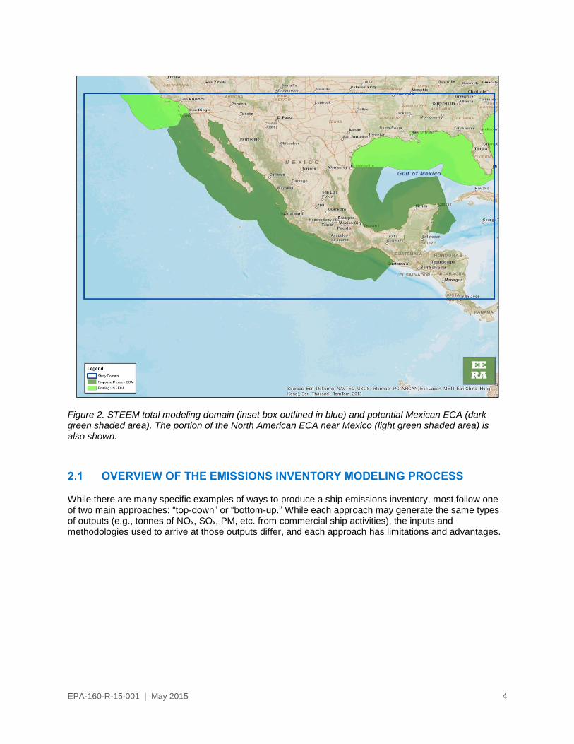
EERA used STEEM to conduct a 2013 emissions inventory that quantifies and then compares ship emissions with and without an ECA. The inventory considered emissions for two areas within the modeling domain: within and outside a potential Mexican ECA. Figure 2 shows the STEEM modeling domain (outlined in the rectangle bounded by a blue line) that was used to create the 2013 inventory. It also shows the U.S. portion of the existing North American ECA near Mexico (light green shaded area) and the potential Mexican ECA (dark green shaded area). Note that the boundary of the Mexican ECA modelled by EERA is 200 nautical miles from the coastline, which matches the boundary formally established for the North American ECA. Results summarize emissions of NOx, SO, PM, black carbon (BC), carbon dioxide (CO2), carbon monoxide (CO) and hydrocarbons (HC) within and outside a potential Mexican ECA for the year 2013, as well as for the year 2030.

EPA-160-R-15-001 | May 2015 4

Figure 2. STEEM total modeling domain (inset box outlined in blue) and potential Mexican ECA (dark green shaded area). The portion of the North American ECA near Mexico (light green shaded area) is also shown.

2.1 OVERVIEW OF THE EMISSIONS INVENTORY MODELING PROCESS

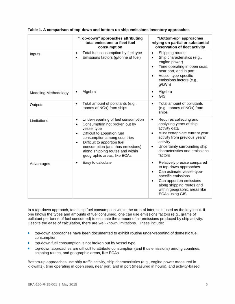
While there are many specific examples of ways to produce a ship emissions inventory, most follow one of two main approaches: “top-down” or “bottom-up.” While each approach may generate the same types of outputs (e.g., tonnes of NOx, SOx, PM, etc. from commercial ship activities), the inputs and methodologies used to arrive at those outputs differ, and each approach has limitations and advantages.

EPA-160-R-15-001 | May 2015 5

Table 1. A comparison of top-down and bottom-up ship emissions inventory approaches

“Top-down” approaches attributing total emissions to fleet fuel

consumption

“Bottom-up” approaches relying on partial or substantial

observation of fleet activity

Inputs Total fuel consumption by fuel type

Emissions factors (g/tonne of fuel)

Shipping routes

Ship characteristics (e.g., engine power)

Time operating in open seas, near port, and in port

Vessel-type-specific emissions factors (e.g., g/kWh)

Modeling Methodology Algebra Algebra

GIS

Outputs Total amount of pollutants (e.g., tonnes of NOx) from ships

Total amount of pollutants (e.g., tonnes of NOx) from ships

Limitations Under-reporting of fuel consumption

Consumption not broken out by vessel type

Difficult to apportion fuel consumption among countries

Difficult to apportion fuel consumption (and thus emissions) along shipping routes and within geographic areas, like ECAs

Requires collecting and analyzing years of ship activity data

Must extrapolate current year activity from previous years’ activity

Uncertainty surrounding ship characteristics and emissions factors

Advantages Easy to calculate Relatively precise compared to top-down approaches

Can estimate vessel-type-specific emissions

Can apportion emissions along shipping routes and within geographic areas like ECAs using GIS

In a top-down approach, total ship fuel consumption within the area of interest is used as the key input. If one knows the types and amounts of fuel consumed, one can use emissions factors (e.g., grams of pollutant per tonne of fuel consumed) to estimate the amount of air emissions produced by ship activity. Despite the ease of calculation, there are well-known limitations. These include:

top-down approaches have been documented to exhibit routine under-reporting of domestic fuel consumption

top-down fuel consumption is not broken out by vessel type

top-down approaches are difficult to attribute consumption (and thus emissions) among countries, shipping routes, and geographic areas, like ECAs

Bottom-up approaches use ship traffic activity, ship characteristics (e.g., engine power measured in kilowatts), time operating in open seas, near port, and in port (measured in hours), and activity-based

EPA-160-R-15-001 | May 2015 6

emission factors (e.g., grams of pollutant per kilowatt-hour) as inputs. While there are some limitations to bottom-up approaches (Table 1), there are clear advantages. These include:

bottom-up approaches can be relatively precise and more accurate compared to top-down approaches

bottom-up approaches can estimate vessel-type-specific emissions (i.e., they can distinguish the amount of air pollutant emissions from container ships, reefers, etc.)

bottom-up approaches can apportion emissions along shipping routes and within geographic areas like ECAs using GIS

There are, of course, limitations to the bottom-up approach, which include:

bottom-up approaches require collecting and analyzing years of ship activity data

bottom-up approaches must extrapolate current year activity from previous years’ activity

bottom-up approaches are subject to uncertainty surrounding ship characteristics (e.g., vessel power in-use along a route) and emissions factors

Despite these limitations, it is important to recognize that no country in the world, including the U.S., has a maritime emissions inventory based entirely on emissions monitoring of the ships operating in its waters. Instead the U.S., other countries, and the IMO now regularly use bottom-up approaches, like STEEM, in developing ship emissions inventories because these methods are recognized as producing reasonable estimates of ship emissions for large coastal areas.

2.2 STEEM

STEEM was constructed as a bottom-up ship emissions inventory that combines ship characteristics including engine power, period of operation (time operating in open seas, near port, and in port), and activity-based emission factors that account for variations in emissions based on vessel type. These bottom-up methods have been peer-reviewed and follow methods described as best practices for commercial marine vessel inventories (U.S. EPA, 2009). The methods are similar to those recommended by the 2006 Intergovernmental Panel on Climate Change (IPCC) Guidelines for Greenhouse Gas Inventories (IPCC, 2006).

Ship routes in STEEM, as shown in Figure 3, are derived from actual ship position reports over a 20-year period to determine where international shipping lanes were located. These ship position reports contained vessel IMO identification numbers used by EERA to determine important characteristics such as vessel type and installed main engine and auxiliary engine power (kW), for vessels traveling along each shipping lane. In earlier work, EERA combined the ship energy use (kW) along each segment of the shipping lanes with the emissions factors in Table 2 to calculate a 2011 ship emissions inventory for Mexico. EERA developed these emissions factors in previous STEEM work (Corbett, 2010).

EPA-160-R-15-001 | May 2015 7

Figure 3. STEEM network representation, including ~1700 World Ports. STEEM estimates emissions from nearly complete historical North American shipping activities and individual ship attributes.

Table 2. Uncontrolled emissions factors (g/kWh) used in 2011 ship emissions inventory calculations

2.3 ESTIMATING 2013 SHIP EMISSIONS

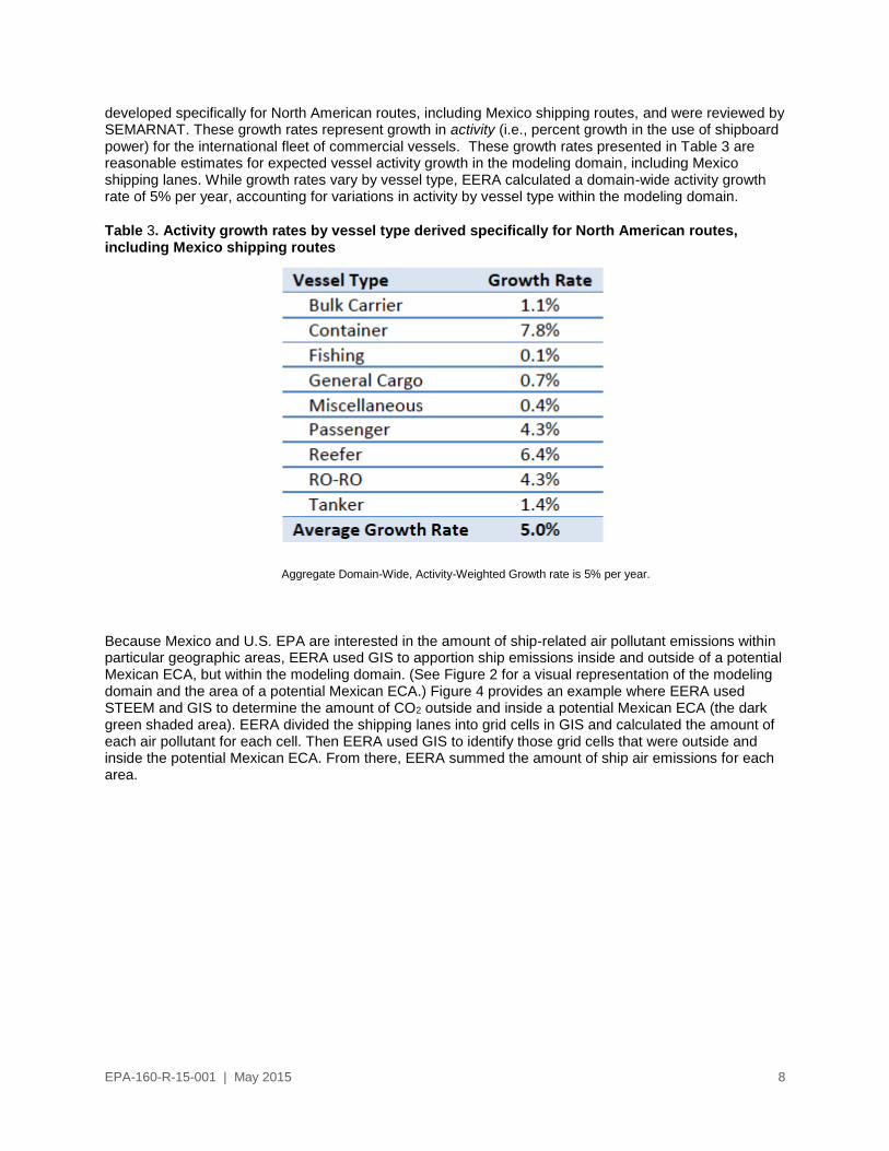
EERA estimated year 2013 ship emissions by multiplying STEEM’s emission estimates for 2011 and the vessel-specific compound annual growth rates for shipping activity shown in Table 3. The emissions factors for 2011 and 2013 were the same because no new national or international maritime emissions control regulations that would reduce pollutant emissions factors went into effect between 2011 and 2013. The growth rates in Table 3 were derived from previous STEEM work (Corbett, 2010) that were

EPA-160-R-15-001 | May 2015 8

developed specifically for North American routes, including Mexico shipping routes, and were reviewed by SEMARNAT. These growth rates represent growth in activity (i.e., percent growth in the use of shipboard power) for the international fleet of commercial vessels. These growth rates presented in Table 3 are reasonable estimates for expected vessel activity growth in the modeling domain, including Mexico shipping lanes. While growth rates vary by vessel type, EERA calculated a domain-wide activity growth rate of 5% per year, accounting for variations in activity by vessel type within the modeling domain.

Table 3. Activity growth rates by vessel type derived specifically for North American routes, including Mexico shipping routes

Aggregate Domain-Wide, Activity-Weighted Growth rate is 5% per year.

Because Mexico and U.S. EPA are interested in the amount of ship-related air pollutant emissions within particular geographic areas, EERA used GIS to apportion ship emissions inside and outside of a potential Mexican ECA, but within the modeling domain. (See Figure 2 for a visual representation of the modeling domain and the area of a potential Mexican ECA.) Figure 4 provides an example where EERA used STEEM and GIS to determine the amount of CO2 outside and inside a potential Mexican ECA (the dark green shaded area). EERA divided the shipping lanes into grid cells in GIS and calculated the amount of each air pollutant for each cell. Then EERA used GIS to identify those grid cells that were outside and inside the potential Mexican ECA. From there, EERA summed the amount of ship air emissions for each area.

EPA-160-R-15-001 | May 2015 9

Figure 4. Example of pairing STEEM with GIS to estimate ship air emissions outside and inside a potential Mexican ECA (dark green shaded area) but within the modeling domain; 2013 CO2 emissions are displayed (dark red represents high emissions).

2.4 ESTIMATING 2030 SHIP EMISSIONS

EERA utilized STEEM results to present two future emissions scenarios for the year 2030. Both scenarios use the vessel-type-specific activity growth rates found in Table 3. The first scenario assumes that a Mexican ECA has not been designated by 2030, and thus uses emissions factors shown in Table 4 that are adjusted to reflect a 0.5% global marine fuel sulfur cap and the globally-applicable NOx marine engine standards established by MARPOL Annex VI. The second scenario assumes that a Mexican ECA is designated prior to 2030 and uses emissions factors that are adjusted to reflect a 0.1% marine fuel sulfur cap and IMO Tier III NOx marine engine standards (Table 5). EERA developed the emissions factors found in Table 4 in previous STEEM work (Corbet, 2010) and reduced the NOx, SOx, and PM emissions factors found in Table 5 to reflect IMO (2008a) Tier III NOx marine engine standards (80% reduction from Tier I) and a 0.1% marine fuel sulfur standard for ships operating in ECAs (IMO, 2008b). (See Appendix I for a summary of key MARPOL Annex VI fuel sulfur limits and marine engine NOx standards.) For emissions within the modeling domain and outside of the already-established North American ECA or the potential Mexican ECA, the emissions factors from Table 4 are applied.

EPA-160-R-15-001 | May 2015 10

Table 4. Emissions factors (g/kWh) for 2030 outside an ECA, reflecting 0.5% fuel sulfur and IMO Tier I NOx marine engine standards

Table 5. Emissions factors (g/kWh) for 2030 within an ECA, reflecting 0.1% fuel sulfur and IMO Tier III NOx marine engine standards

2.5 PORT EMISSIONS

While emissions from ships in ports were used in addition to STEEM in developing the North American marine emissions inventory, EERA did not do so in developing the initial 2011 Mexican marine emissions inventory. No national-scale inventory of ship emissions in ports in Mexico was known to exist at the time of EERA’s work, and SEMARNAT officials agreed to proceed on this task without one. Moreover, EERA, Battelle, SEMARNAT, and U.S. EPA concluded that the addition of national port ship emissions data for Mexico would make a very marginal difference to the overall results of this marine emissions inventory. Further, EERA, Battelle, SEMARNAT, and U.S. EPA determined that the 2011 Mexican marine emissions inventory would provide Mexico with sufficient information to demonstrate that ships operating in the proposed area of application are contributing to ambient concentrations of air pollution or to adverse environmental impacts, including human health impacts, if they prepared an ECA designation proposal for IMO. This does not mean, however, that port emissions are irrelevant in terms of air quality, public health and the environment in local areas, as demonstrated in many port areas around the world. In a separate effort, the CEC has developed an emission inventory approach for future updates to ship emissions as part of the national emission inventory that will include Mexican ship emissions while in port (CEC, 2015).

EPA-160-R-15-001 | May 2015 11

3.0 Results

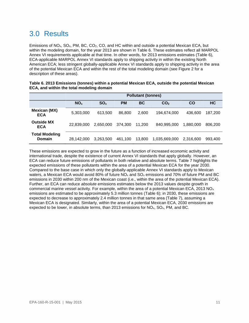
Emissions of NOx, SOx, PM, BC, CO2, CO, and HC within and outside a potential Mexican ECA, but within the modeling domain, for the year 2013 are shown in Table 6. These estimates reflect all MARPOL Annex VI requirements applicable at that time. In other words, for 2013 emissions estimates (Table 6), ECA-applicable MARPOL Annex VI standards apply to shipping activity in within the existing North American ECA; less stringent globally-applicable Annex VI standards apply to shipping activity in the area of the potential Mexican ECA and within the rest of the total modeling domain (see Figure 2 for a description of these areas).

Table 6. 2013 Emissions (tonnes) within a potential Mexican ECA, outside the potential Mexican ECA, and within the total modeling domain

Pollutant (tonnes)

NOx SOx PM BC CO2 CO HC

Mexican (MX) ECA

5,303,000 613,500 86,800 2,600 194,674,000 436,600 187,200

Outside MX ECA

22,839,000 2,650,000 374,300 11,200 840,995,000 1,880,000 806,200

Total Modeling Domain 28,142,000 3,263,500 461,100 13,800 1,035,669,000 2,316,600 993,400

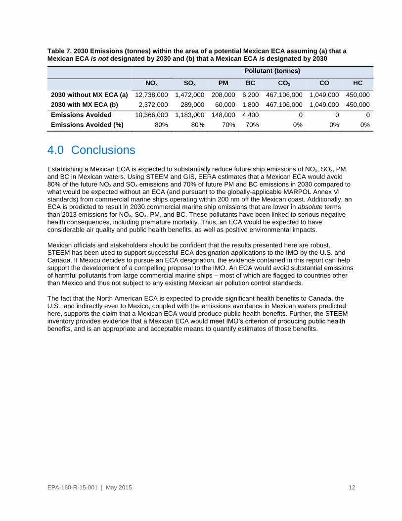
These emissions are expected to grow in the future as a function of increased economic activity and international trade, despite the existence of current Annex VI standards that apply globally. However, an ECA can reduce future emissions of pollutants in both relative and absolute terms. Table 7 highlights the expected emissions of these pollutants within the area of a potential Mexican ECA for the year 2030. Compared to the base case in which only the globally-applicable Annex VI standards apply to Mexican waters, a Mexican ECA would avoid 80% of future NOx and SOx emissions and 70% of future PM and BC emissions in 2030 within 200 nm of the Mexican coast (i.e., within the area of the potential Mexican ECA). Further, an ECA can reduce absolute emissions estimates below the 2013 values despite growth in commercial marine vessel activity. For example, within the area of a potential Mexican ECA, 2013 NOx emissions are estimated to be approximately 5.3 million tonnes (Table 6); in 2030, these emissions are expected to decrease to approximately 2.4 million tonnes in that same area (Table 7), assuming a Mexican ECA is designated. Similarly, within the area of a potential Mexican ECA, 2030 emissions are expected to be lower, in absolute terms, than 2013 emissions for NOx, SOx, PM, and BC.

EPA-160-R-15-001 | May 2015 12

Table 7. 2030 Emissions (tonnes) within the area of a potential Mexican ECA assuming (a) that a Mexican ECA is not designated by 2030 and (b) that a Mexican ECA is designated by 2030

Pollutant (tonnes)

NOx SOx PM BC CO2 CO HC

2030 without MX ECA (a) 12,738,000 1,472,000 208,000 6,200 467,106,000 1,049,000 450,000

2030 with MX ECA (b) 2,372,000 289,000 60,000 1,800 467,106,000 1,049,000 450,000

Emissions Avoided 10,366,000 1,183,000 148,000 4,400 0 0 0

Emissions Avoided (%) 80% 80% 70% 70% 0% 0% 0%

4.0 Conclusions

Establishing a Mexican ECA is expected to substantially reduce future ship emissions of NOx, SOx, PM, and BC in Mexican waters. Using STEEM and GIS, EERA estimates that a Mexican ECA would avoid 80% of the future NOx and SOx emissions and 70% of future PM and BC emissions in 2030 compared to what would be expected without an ECA (and pursuant to the globally-applicable MARPOL Annex VI standards) from commercial marine ships operating within 200 nm off the Mexican coast. Additionally, an ECA is predicted to result in 2030 commercial marine ship emissions that are lower in absolute terms than 2013 emissions for NOx, SOx, PM, and BC. These pollutants have been linked to serious negative health consequences, including premature mortality. Thus, an ECA would be expected to have considerable air quality and public health benefits, as well as positive environmental impacts.

Mexican officials and stakeholders should be confident that the results presented here are robust. STEEM has been used to support successful ECA designation applications to the IMO by the U.S. and Canada. If Mexico decides to pursue an ECA designation, the evidence contained in this report can help support the development of a compelling proposal to the IMO. An ECA would avoid substantial emissions of harmful pollutants from large commercial marine ships – most of which are flagged to countries other than Mexico and thus not subject to any existing Mexican air pollution control standards.

The fact that the North American ECA is expected to provide significant health benefits to Canada, the U.S., and indirectly even to Mexico, coupled with the emissions avoidance in Mexican waters predicted here, supports the claim that a Mexican ECA would produce public health benefits. Further, the STEEM inventory provides evidence that a Mexican ECA would meet IMO’s criterion of producing public health benefits, and is an appropriate and acceptable means to quantify estimates of those benefits.

EPA-160-R-15-001 | May 2015 13

5.0 References

Commission for Environmental Cooperation (CEC). 2015. Reducing emissions from goods movement via

maritime transportation in North America: Update of the Mexican port emissions data – Draft for

review. Montreal: CEC.

Corbett, J.J. 2010. Improved geospatial scenarios for commercial marine vessels. Sacramento, CA:

California Air Resources Board and the California Environmental Protection Agency.

Intergovernmental Panel on Climate Change (IPCC). 2006. Chapter 3: Mobile combustion. In IPCC, 2006

Guidelines for national greenhouse gas inventories, Volume 2: Energy. Prepared by the National

Greenhouse Gas Inventories Programme, Eggleston, H.S., Buendia, L., Miwa, K., Ngara, T., and

Tanabe, K. (eds). Japan: IGES.

International Maritime Organization (IMO). 2008a. Nitrogen oxides (NOx) – Regulation 13. In MEPC

58/23/Add.1, Annex 13: Resolution MEPC.176 (58). London: IMO.

International Maritime Organization (IMO). 2008b. Sulfur oxides (SOx) – Regulation 14. In MEPC

58/23/Add.1, Annex 13: Resolution MEPC.176 (58). London: IMO.

Mexico Secretary of Environment and Natural Resources (SEMARNAT). 2013. Work plan and strategy for

technical analyses needed for MARPOL Annex VI ratification and development of an ECA

proposal.

U.S. Environmental Protection Agency (U.S. EPA). 2009. Current methodologies in preparing mobile

source port-related emission inventories final report. Prepared by ICF International. Washington,

DC: U.S. EPA. Report No: 09-024

EPA-160-R-15-001 | May 2015 A I-1

APPENDIX I: Key MARPOL Annex VI Standards (Global

and ECA)

Fuel sulfur limit (sulfur content cap) (from Regulation 14 of MARPOL Annex VI)

Applicability Effective Date Sulfur Limit Comment

Global Prior to 1 Jan. 2012

As of 1 Jan. 2012

As of 1 Jan. 2020 (*)

4.5% (45,000 ppm)

3.5% (35,000 ppm)

0.5% (5,000 ppm)

Applies to all ships

*subject to feasibility review in 2018, could delay effective date to 2025

ECA 1 July 2010

1 Jan. 2015

1.0% (10,000 ppm)

0.1% (1,000 ppm)

NOx marine engine emission standards (from Regulation 13 of MARPOL Annex VI)

Applicability Effective Date NOx Limit Comment

Global 1 Jan. 2000

1 Jan. 2011

Tier 1

Tier 2: ~20% reduction below Tier 1 for new vessels

Applies to marine diesel engines on ships constructed on or after this date

Applies to ships constructed on or after this date

ECA 1 Jan 2016 Tier 3: 80% reduction below Tier 1 for new vessels

Applies to ships built as of 2016 when they operate in the North American and U.S. Caribbean Sea ECAs.

EPA-160-R-15-001 | May 2015 A II-1

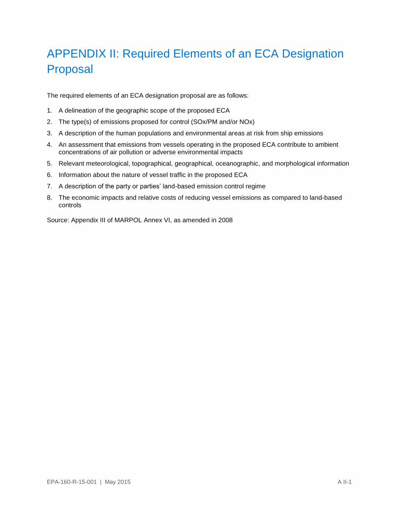
APPENDIX II: Required Elements of an ECA Designation

Proposal

The required elements of an ECA designation proposal are as follows: 1. A delineation of the geographic scope of the proposed ECA

2. The type(s) of emissions proposed for control (SOx/PM and/or NOx)

3. A description of the human populations and environmental areas at risk from ship emissions

4. An assessment that emissions from vessels operating in the proposed ECA contribute to ambient concentrations of air pollution or adverse environmental impacts

5. Relevant meteorological, topographical, geographical, oceanographic, and morphological information

6. Information about the nature of vessel traffic in the proposed ECA

7. A description of the party or parties’ land-based emission control regime

8. The economic impacts and relative costs of reducing vessel emissions as compared to land-based controls

Source: Appendix III of MARPOL Annex VI, as amended in 2008

EPA-160-R-15-001 | May 2015 AIII-1

APPENDIX III: 2011 Ship Emission Inventory Results

EPA-160-R-15-001 | May 2015 A III-2

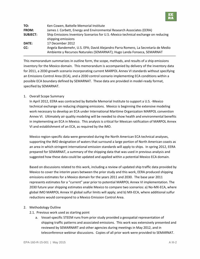
TO: Ken Cowen, Battelle Memorial Institute FROM: James J. Corbett, Energy and Environmental Research Associates (EERA) SUBJECT: Ship Emissions Inventory Scenarios for U.S.-Mexico technical exchange on reducing

shipping emissions DATE: 17 December 2012 CC: Angela Bandemehr, U.S. EPA; David Alejandro Parra Romero, La Secretaría de Medio

Ambiente y Recursos Naturales (SEMARNAT); Hugo Landa Fonseca, SEMARNAT This memorandum summarizes in outline form, the scope, methods, and results of a ship emissions

inventory for the Mexico domain. This memorandum is accompanied by delivery of the inventory data

for 2011, a 2030 growth scenario incorporating current MARPOL Annex VI standards without specifying

an Emissions Control Area (ECA), and a 2030 control scenario implementing ECA conditions within a

possible ECA boundary defined by SEMARNAT. These data are provided in model-ready format,

specified by SEMARNAT.

1. Overall Scope Summary

In April 2012, EERA was contracted by Battelle Memorial Institute to support a U.S. -Mexico

technical exchange on reducing shipping emissions. Mexico is beginning the extensive modeling

work necessary to develop an ECA under International Maritime Organization MARPOL convention

Annex VI. Ultimately air quality modeling will be needed to show health and environmental benefits

in implementing an ECA in Mexico. This analysis is critical for Mexican ratification of MARPOL Annex

VI and establishment of an ECA, as required by the IMO.

Mexico region-specific data were generated during the North American ECA technical analyses,

supporting the IMO designation of waters that surround a large portion of North American coasts as

an area in which stringent international emission standards will apply to ships. In spring 2012, EERA

prepared for SEMARNAT, a summary of the shipping data that was used in previous analysis and

suggested how these data could be updated and applied within a potential Mexico ECA domain.

Based on discussions related to this work, including a review of updated ship traffic data provided by

Mexico to cover the interim years between the prior study and this work, EERA produced shipping

emissions estimates for a Mexico domain for the years 2011 and 2030. The base year 2011

represents estimates for a “current” year prior to potential MARPOL Annex VI implementation. The

2030 future year shipping estimates enable Mexico to compare two scenarios: a) No-MX-ECA, where

global IMO MARPOL Annex VI global sulfur limits will apply; and b) MX-ECA, where additional sulfur

reductions would correspond to a Mexico Emission Control Area.

2. Methodology Outline

2.1. Previous work used as starting point

a. Vessel-specific STEEM runs from prior study provided a geospatial representation of

shipping traffic patterns and associated emissions. This work was extensively presented and

reviewed by SEMARNART and other agencies during meetings in May 2012, and in

teleconference webinar discussions. Copies of all prior work were provided to SEMARNAT.

EPA-160-R-15-001 | May 2015 A III-3

b. Defined domain for Mexico analysis, with approval from SEMARNAT staff

a. GIS projection used the existing GCS_WGS_1984, to be converted prior to

transmittal

b. Top (north boundary): 35.00 decimal degrees

c. Bottom (south boundary): 10.00 decimal degrees

d. Left (west boundary): -130.00 decimal degrees

e. Right (east boundary): -80.00 decimal degrees

c. Per request from SEMARNAT, we redefined the grid size for output

a. grid cells are 0.25 degrees x 0.25 degrees on GCS WGS84

b. grid cells are approximately 28 kilometer x 28 kilometer at center of domain

c. final output will be re-projected to desired coordinate system for modeling,

specified as Lambert Conformal by SEMARNAT

2.2. Updated Emissions Rates

a. Based on current IMO MARPOL VI legislation, emissions limits applying to non-ECA regions

and to ECA regions will become progressively stricter over the next two decades. Table 1

shows the MARPOL Annex VI limits for oxides of sulfur.

Table 8. Present and upcoming fuel oil sulfur limits inside and outside ECAs

Outside an ECA Inside an ECA

4.50% m/m prior to 1 January 2012 1.50% m/m prior to 1 July 2010

3.50% m/m on and after 1 January 2012 1.00% m/m on and after 1 July 2010

0.50% m/m on and after 1 January 2020* 0.10% m/m on and after 1 January 2015

*depending on the outcome of a review, to be concluded in 2018, as to the availability of the required fuel oil, this date could be deferred to 1 January 2025.

b. Emissions in 2011 are shown in Table 2. These rates are taken directly from the previous

analysis for the North American ECA application, and applied to estimate 2011 inventory for

this work. Black Carbon emissions rates are proportional to total PM rates, although the

literature reports a range of typical proportions. For Vessels that are uncontrolled for PM

currently, we use a BC:PM ratio of approximately 3%, per the U.S. EPA Report to Congress

on Black Carbon (2012), by Sauser E., Hemby J., Adler K., e al.

Table 9. Summary of uncontrolled emissions factor in 2002, 2010 (g/kWh).

Vessel Type NOx SOx CO2 HC PM CO

Bulk 17.9 10.6 622.9 0.6 1.5 1.4

Container 17.9 10.6 622.9 0.6 1.5 1.4

Fishing 14 11.5 677 0.5 1.5 1.1

General 17.9 10.6 622.9 0.6 1.5 1.4

Miscellaneous 14 11.5 677 0.5 1.5 1.1

Passenger 17.9 10.6 622.9 0.6 1.5 1.4

Reefer 17.9 10.6 622.9 0.6 1.5 1.4

RO-RO 17.9 10.6 622.9 0.6 1.5 1.4

Tanker 17.9 10.6 622.9 0.6 1.5 1.4

EPA-160-R-15-001 | May 2015 A III-4

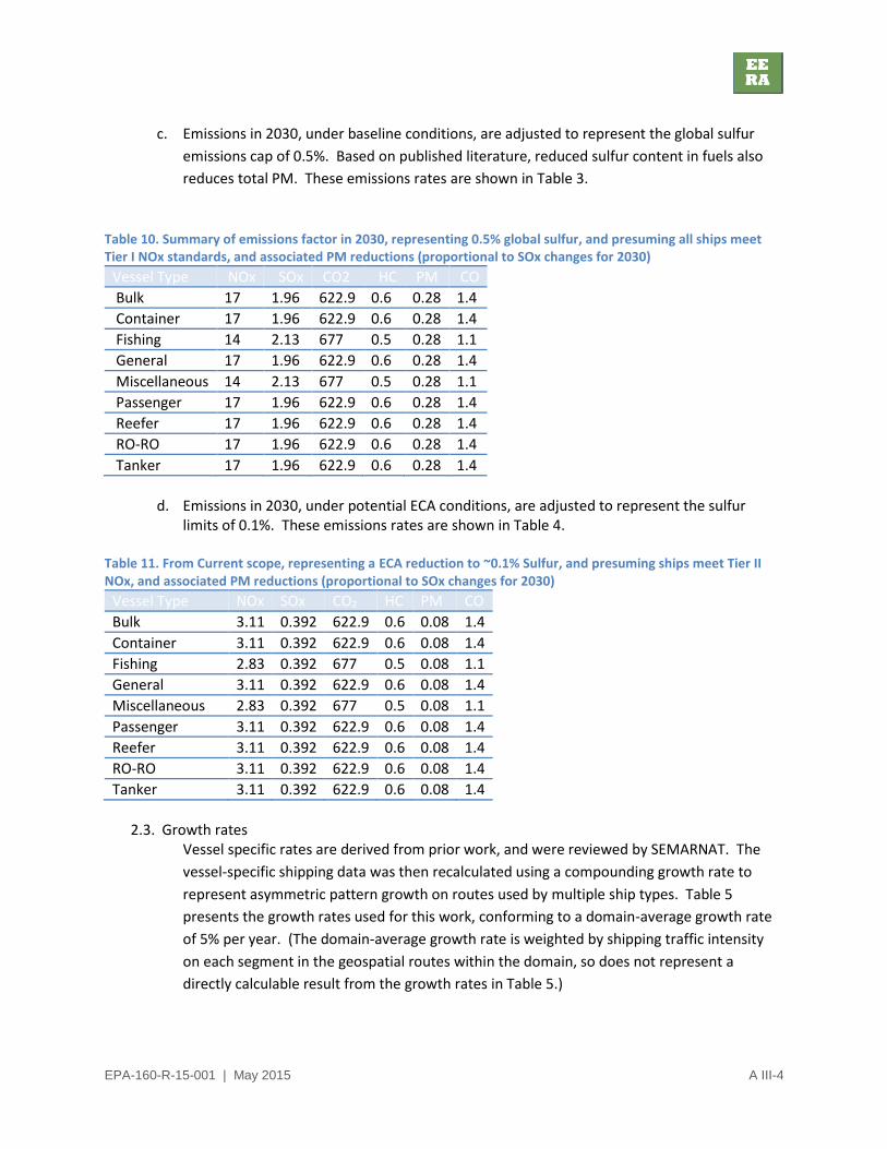
c. Emissions in 2030, under baseline conditions, are adjusted to represent the global sulfur

emissions cap of 0.5%. Based on published literature, reduced sulfur content in fuels also

reduces total PM. These emissions rates are shown in Table 3.

Table 10. Summary of emissions factor in 2030, representing 0.5% global sulfur, and presuming all ships meet Tier I NOx standards, and associated PM reductions (proportional to SOx changes for 2030)


Bulk 17 1.96 622.9 0.6 0.28 1.4

Container 17 1.96 622.9 0.6 0.28 1.4

Fishing 14 2.13 677 0.5 0.28 1.1

General 17 1.96 622.9 0.6 0.28 1.4

Miscellaneous 14 2.13 677 0.5 0.28 1.1

Passenger 17 1.96 622.9 0.6 0.28 1.4

Reefer 17 1.96 622.9 0.6 0.28 1.4

RO-RO 17 1.96 622.9 0.6 0.28 1.4

Tanker 17 1.96 622.9 0.6 0.28 1.4

d. Emissions in 2030, under potential ECA conditions, are adjusted to represent the sulfur

limits of 0.1%. These emissions rates are shown in Table 4. Table 11. From Current scope, representing a ECA reduction to ~0.1% Sulfur, and presuming ships meet Tier II NOx, and associated PM reductions (proportional to SOx changes for 2030)


Bulk 3.11 0.392 622.9 0.6 0.08 1.4

Container 3.11 0.392 622.9 0.6 0.08 1.4

Fishing 2.83 0.392 677 0.5 0.08 1.1

General 3.11 0.392 622.9 0.6 0.08 1.4

Miscellaneous 2.83 0.392 677 0.5 0.08 1.1

Passenger 3.11 0.392 622.9 0.6 0.08 1.4

Reefer 3.11 0.392 622.9 0.6 0.08 1.4

RO-RO 3.11 0.392 622.9 0.6 0.08 1.4

Tanker 3.11 0.392 622.9 0.6 0.08 1.4

2.3. Growth rates

Vessel specific rates are derived from prior work, and were reviewed by SEMARNAT. The

vessel-specific shipping data was then recalculated using a compounding growth rate to

represent asymmetric pattern growth on routes used by multiple ship types. Table 5

presents the growth rates used for this work, conforming to a domain-average growth rate

of 5% per year. (The domain-average growth rate is weighted by shipping traffic intensity

on each segment in the geospatial routes within the domain, so does not represent a

directly calculable result from the growth rates in Table 5.)

EPA-160-R-15-001 | May 2015 A III-5

Table 12. Summary of growth rate calculations supporting a regional compound average growth rate ~5%.

Vessel Type Growth Rate

Bulk Carrier 1.1%

Container 7.8%

Fishing 0.1%

General Cargo 0.7%

Miscellaneous 0.4%

Passenger 4.3%

Reefer 6.4%

RO-RO 4.3%

Tanker 1.4%

Average Growth Rate 5.0% 3. Results

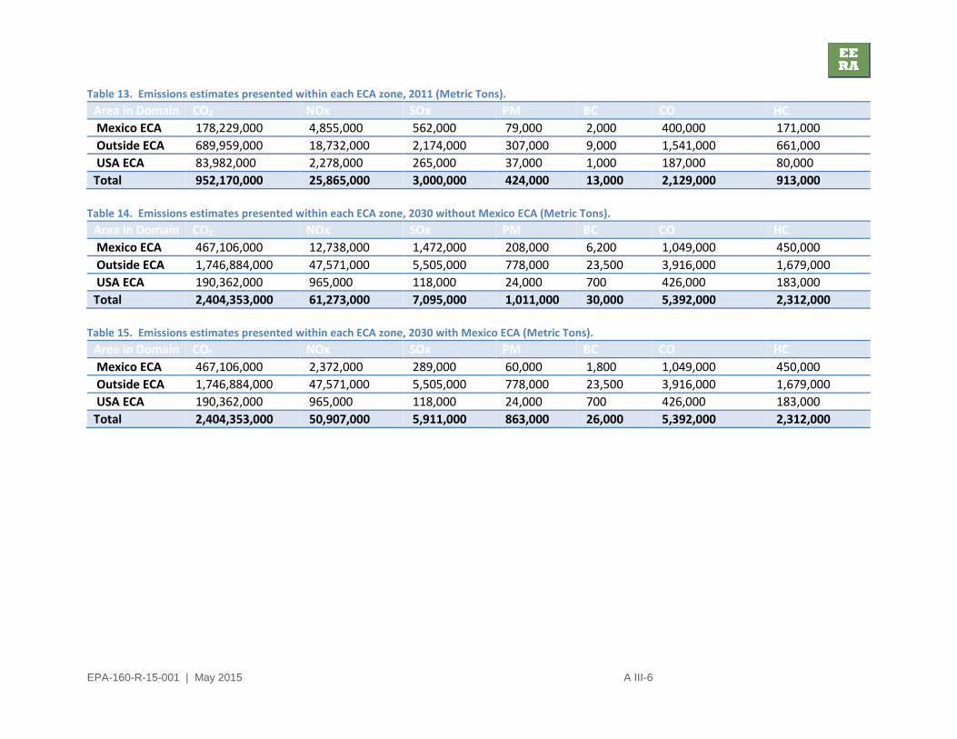
The application of growth rates mentioned in previous sections defines emissions estimates for

2011 and 2030. Table 6 presents emissions totals for 2011. Table 7 presents emissions totals

for 2030, without adjusted emissions representing control under a Mexico ECA. Table 8

presents emissions totals for 2030, including reductions for those areas that conform to

expected ECA controls and no reductions for those areas not expected to conform that fall

within a Mexico domain.

These totals are identified by whether they fall within the potential Mexico ECA, within the

current U.S. ECA, or outside an ECA domain. Comparing Table 7 and Table 8, one can see that

the US ECA region remains unchanged (controlled within ECA limits in both scenarios); similarly,

the area outside ECA control is unchanged, conforming only to global MARPOL Annex VI

standards, applicable to oxides of sulfur, oxides of NOx, and PM (with BC a subset of PM).

Additionally, one can observe that controlled emissions within the Mexico ECA in 2030 after

growth escalation are lower than uncontrolled emissions in 2011. This demonstrates significant

potential reductions attributed to a Mexico ECA designation in coastal waters surrounding

Mexico.

All emissions values are presented in the gridded data file for modeling with columns for X and Y

coordinates indicating point location, additional columns designating estimated emissions and

rows representing each point.

EPA-160-R-15-001 | May 2015 A III-6

Table 13. Emissions estimates presented within each ECA zone, 2011 (Metric Tons).

Area in Domain CO2 NOx SOx PM BC CO HC

Mexico ECA 178,229,000 4,855,000 562,000 79,000 2,000 400,000 171,000

Outside ECA 689,959,000 18,732,000 2,174,000 307,000 9,000 1,541,000 661,000

USA ECA 83,982,000 2,278,000 265,000 37,000 1,000 187,000 80,000

Total 952,170,000 25,865,000 3,000,000 424,000 13,000 2,129,000 913,000

Table 14. Emissions estimates presented within each ECA zone, 2030 without Mexico ECA (Metric Tons).

Area in Domain CO2 NOx SOx PM BC CO HC

Mexico ECA 467,106,000 12,738,000 1,472,000 208,000 6,200 1,049,000 450,000

Outside ECA 1,746,884,000 47,571,000 5,505,000 778,000 23,500 3,916,000 1,679,000

USA ECA 190,362,000 965,000 118,000 24,000 700 426,000 183,000

Total 2,404,353,000 61,273,000 7,095,000 1,011,000 30,000 5,392,000 2,312,000

Table 15. Emissions estimates presented within each ECA zone, 2030 with Mexico ECA (Metric Tons).

Area in Domain COf NOx SOx PM BC CO HC

Mexico ECA 467,106,000 2,372,000 289,000 60,000 1,800 1,049,000 450,000

Outside ECA 1,746,884,000 47,571,000 5,505,000 778,000 23,500 3,916,000 1,679,000

USA ECA 190,362,000 965,000 118,000 24,000 700 426,000 183,000

Total 2,404,353,000 50,907,000 5,911,000 863,000 26,000 5,392,000 2,312,000

EPA-160-R-15-001 | May 2015 A III-7

The prior work used as a basis for this work included port-call data specific to each nation (U.S., Canada,

and Mexico). Thus, we can evaluate the underlying information to estimate emissions proportions by

these nations. These are indicative only – i.e., the national shares are not certain, given the assumed

constancy of shipping patterns, the use of constant growth rates, etc. Table 9-11 presents proportional,

speciated emissions for these nations. Totals for all emissions data are presented in the gridded data

file, after merging the nation-by-nation data into a single value representing each grid point for

modeling.

Table 16. Summary of SOx emissions estimated for 2030 ECA scenario (Metric Tons).

Nation and Vessel Type Mexico ECA USA ECA Outside ECA Total

Mexico 81,000 587,000 860 669,000

USA 193,000 4,765,000 116,000 5,075,000

Canada 14,000 153,000 450 168,000

Total 289,000 5,505,000 118,000 5,911,000 Table 17. Summary of NOx emissions estimated for 2030 ECA scenario (Metric Tons).


Mexico 666,000 5,082,000 7,100 5,755,000

USA 1,588,000 41,172,000 954,000 43,714,000

Canada 119,000 1,316,000 3,700 1,439,000

Total 2,372,000 47,571,000 965,000 50,907,000 Table 18. Summary of PM emissions estimated for 2030 ECA scenario (Metric Tons).


Mexico 17,000 83,000 180 100,000

USA 40,000 674,000 24,000 738,000

Canada 3,000 22,000 90 25,000

Total 60,000 778,000 24,000 863,000

For clarity in transmittal, we present a selected set of maps to visualize the results presented in

the new data across the entire study domain. These maps are to be used for understanding the

data as a whole, rather than pinpointing specific emissions. Maps are reproduced full size at the

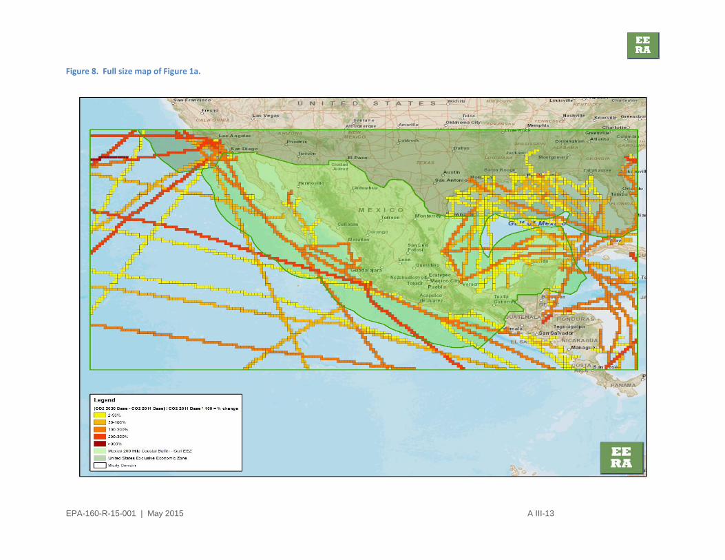
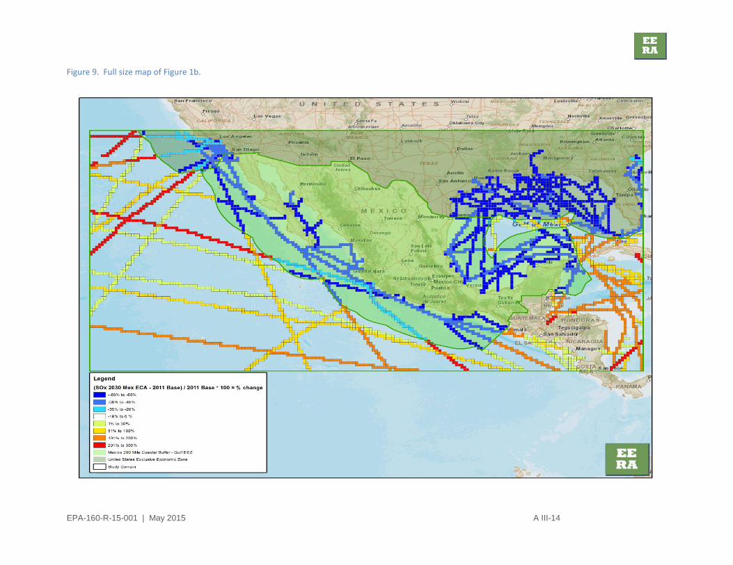
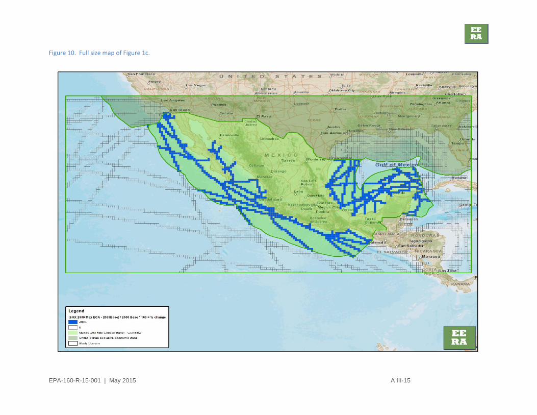
end of this memorandum. Figure 1 illustrates several key comparisons in three panels:

a. the percent change (increase) in energy use and/or CO2 emissions attributed to growth in

shipping within the domain.

b. the percent change (increase in warm colors, decrease in cool colors) in SOx emissions

attributed to both a growth in shipping activity and implementation of sulfur emissions

controls to comply with MARPOL Annex VI limits within a Mexico ECA.

c. the percent change in sulfur emissions between a scenario in which no-ECA condition is

adopted in 2030 and a scenario in which a Mexico ECA is designated.

EPA-160-R-15-001 | May 2015 A III-8

a) b)

c)

Figure 5. Change in emissions produced by 2030 Mexico ECA scenario compared with a) 2011 energy and CO2 emissions; b) 2011 SOx emissions; and c) 2030 Baseline Scenario emissions.

EPA-160-R-15-001 | May 2015 A III-9

a)

b)

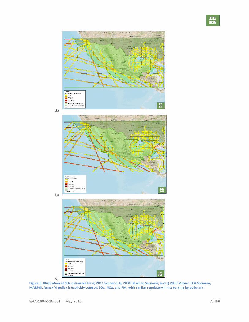
c) Figure 6. Illustration of SOx estimates for a) 2011 Scenario; b) 2030 Baseline Scenario; and c) 2030 Mexico ECA Scenario; MARPOL Annex VI policy is explicitly controls SOx, NOx, and PM, with similar regulatory limits varying by pollutant.

EPA-160-R-15-001 | May 2015 A III-10

a)

b)

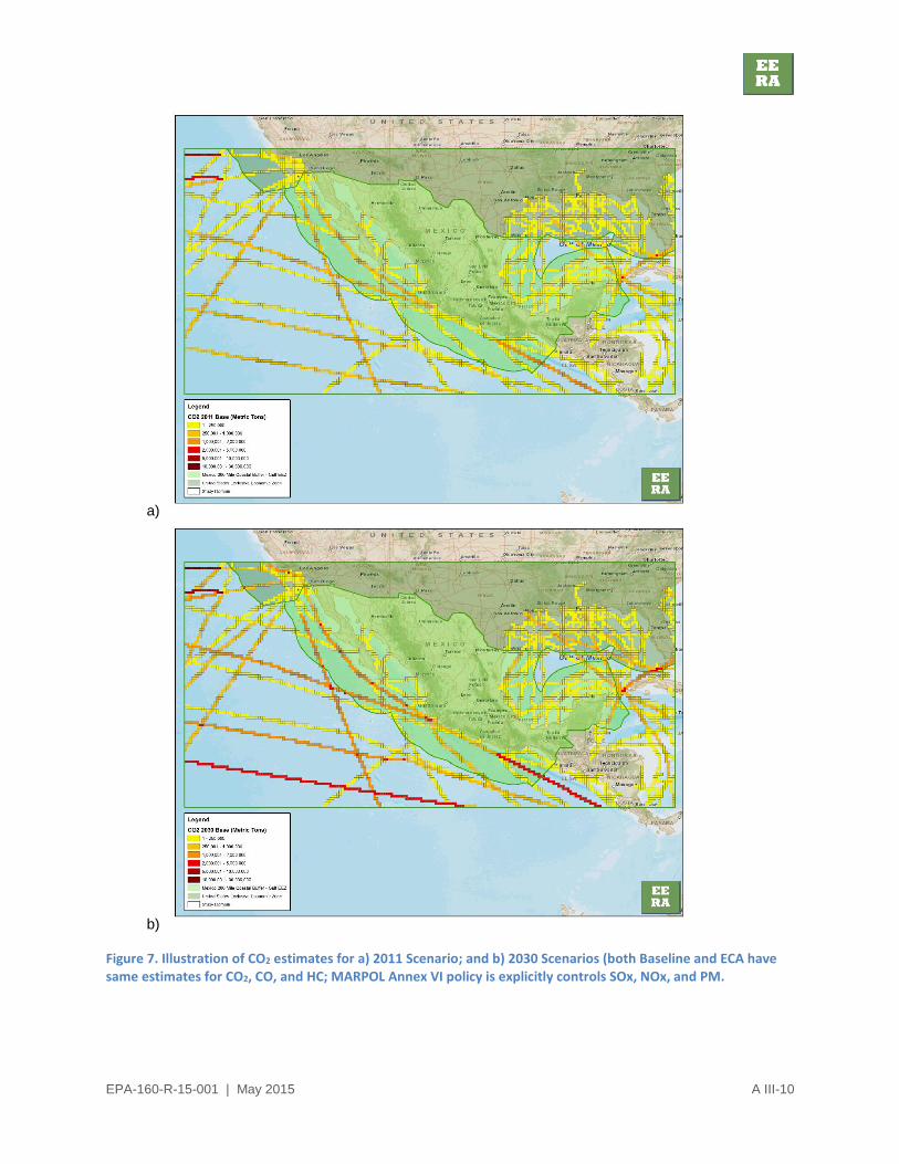
Figure 7. Illustration of CO2 estimates for a) 2011 Scenario; and b) 2030 Scenarios (both Baseline and ECA have same estimates for CO2, CO, and HC; MARPOL Annex VI policy is explicitly controls SOx, NOx, and PM.

EPA-160-R-15-001 | May 2015 A III-11

a. Study assumption biases and limitations mostly relate to well-documented conditions underlying

the data used in prior studies, or the adjustments made for this inventory. Table 12 presents a

summary of potential impacts that may be associated with additional information, not addressed

in this inventory methodology. The degree by which combinations of these conditions may affect

the inventory values is not quantifiable within the methods followed here. However, these

conditions are largely similar to those in the successful North American ECA for the U.S. and

Canada. In fact, by holding these conditions constant, the potential impact (benefit) of reduced

emissions from ships can be directly evaluated.

Table 19. Summary of key conditions that could affect the inventory scenario results.

Conditions that may bias the inventory lower

Conditions with unquantified or unknown inventory bias

Conditions that may bias the inventory higher

Investment in new port capacity that attracts new volume

Shifting shipping patterns due to emerging markets

Change in vessel speed, i.e., slow steaming operations

Vessels transiting Panama Canal without calling on North America

Constrained source of compliant fuels; expanded use of after-treatment

Fleet modernization efficiencies reducing fuel use

1. Deliverable details

Layout and resolution for the delivered data set will use a Lambert conformal resolution, per

specification by SEMARNAT. Among various Lambert projections in ESRI GIS tools we are

using, we confirmed with SEMARNAT that a projection using “North America Lambert Conformal

Conic” meets specifications (see http://spatialreference.org/ref/esri/102009/).

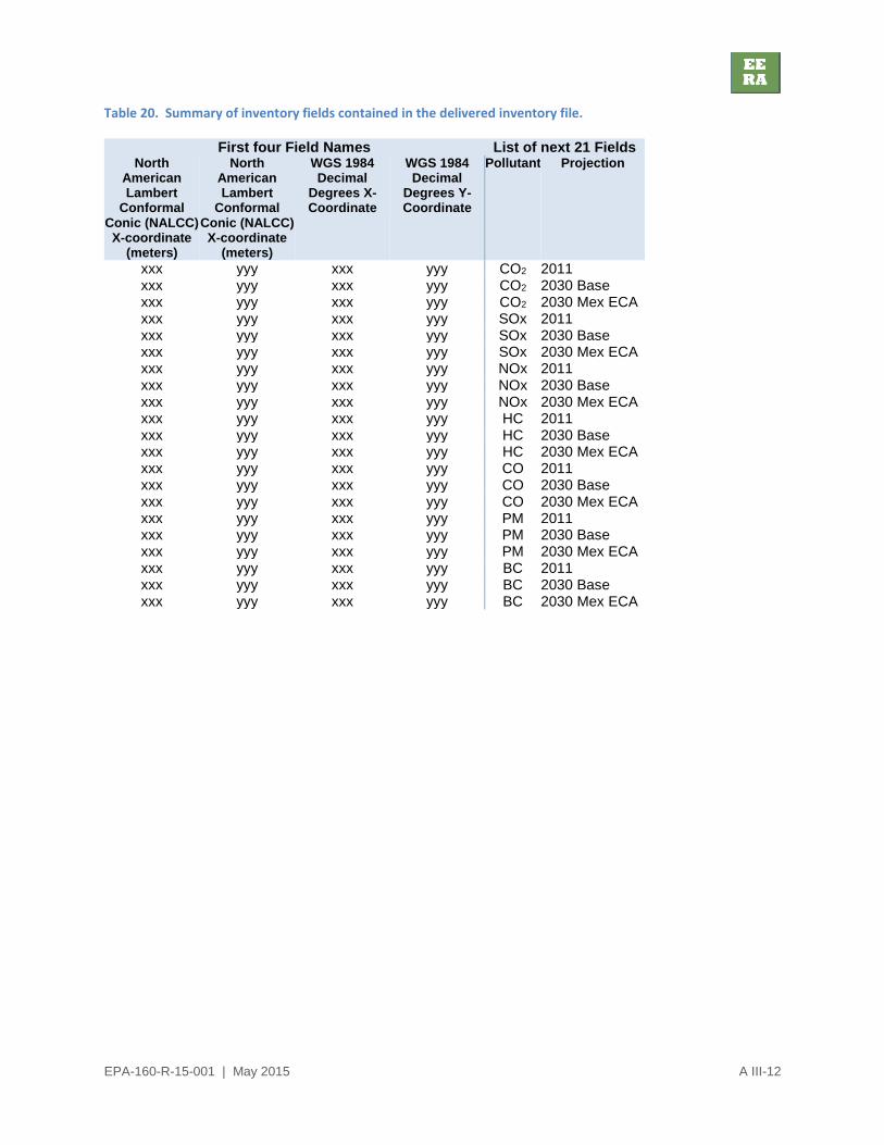
Fields in inventory files will include those identified in Table 13. Essentially there will be twenty-

seven data columns, three scenarios for each of seven pollutants. These are geo-located using

x- and y-coordinates appropriate to the specified projection.

With these inventories, modelers can evaluate fate and transport of emissions including shipping

within the domain, and compute the difference between 2030 scenarios with and without ECA

emissions reductions.

http://spatialreference.org/ref/esri/102009/

EPA-160-R-15-001 | May 2015 A III-12

Table 20. Summary of inventory fields contained in the delivered inventory file.

First four Field Names List of next 21 Fields North

American Lambert

Conformal Conic (NALCC) X-coordinate

(meters)

North American Lambert

Conformal Conic (NALCC) X-coordinate

(meters)

WGS 1984 Decimal

Degrees X-Coordinate

WGS 1984 Decimal

Degrees Y-Coordinate

Pollutant Projection

xxx yyy xxx yyy CO2 2011 xxx yyy xxx yyy CO2 2030 Base xxx yyy xxx yyy CO2 2030 Mex ECA xxx yyy xxx yyy SOx 2011 xxx yyy xxx yyy SOx 2030 Base xxx yyy xxx yyy SOx 2030 Mex ECA xxx yyy xxx yyy NOx 2011 xxx yyy xxx yyy NOx 2030 Base xxx yyy xxx yyy NOx 2030 Mex ECA xxx yyy xxx yyy HC 2011 xxx yyy xxx yyy HC 2030 Base xxx yyy xxx yyy HC 2030 Mex ECA xxx yyy xxx yyy CO 2011 xxx yyy xxx yyy CO 2030 Base xxx yyy xxx yyy CO 2030 Mex ECA xxx yyy xxx yyy PM 2011 xxx yyy xxx yyy PM 2030 Base xxx yyy xxx yyy PM 2030 Mex ECA xxx yyy xxx yyy BC 2011 xxx yyy xxx yyy BC 2030 Base xxx yyy xxx yyy BC 2030 Mex ECA

EPA-160-R-15-001 | May 2015 A III-13

Figure 8. Full size map of Figure 1a.

EPA-160-R-15-001 | May 2015 A III-14

Figure 9. Full size map of Figure 1b.

EPA-160-R-15-001 | May 2015 A III-15

Figure 10. Full size map of Figure 1c.

EPA-160-R-15-001 | May 2015 A III-16


EPA-160-R-15-001 | May 2015 A III-17


EPA-160-R-15-001 | May 2015 A III-18

Figure 13. Full size map of Figure 2c.

EPA-160-R-15-001 | May 2015 A III-19


EPA-160-R-15-001 | May 2015 A III-20


us mexico cooperation on reducing emissions from ships through

Documents