Japan and the World Economy 22 (2010) 98–106

US external debt sustainability revisited: Bayesian analysis of extended Markovswitching unit root test

Fumihide Takeuchi *

Economic Research Department, Japan Center for Economic Research, 1-3-7 Otemachi, Chiyoda-ku, Tokyo 100-8066, Japan

A R T I C L E I N F O

Article history:

Received 1 August 2008

Received in revised form 12 August 2009

Accepted 21 December 2009

JEL classification:

C11

C22

F21

F32

Keywords:

US external debt sustainability

Markov switching unit root test

A B S T R A C T

The sustainability of US external debt, which has been an issue of global concern, is analyzed using a

Markov switching (MS) unit root test applied to the flow of debt, i.e., the current account. The first to

apply the MS unit root test to the issue of US external debt in order to examine local stationarity and

global stationarity were Raybaudi et al. (2004). This paper introduces an extended MS unit root test

where the transition probability is time-varying rather than fixed, as is usually the case, and the change

of probability is explained by the real exchange rate, which theory suggests has a close relationship with

the external balance. The extended MS unit root test calculated by the Markov Chain Monte Carlo

(MCMC) method provides us with new insights on the issue of US external debt in recent years,

suggesting that even though the debt/current account–GDP ratio remains relatively high, the probability

of stationarity (sustainability) is unexpectedly high when recent US dollar depreciation is taken into

account.

� 2010 Elsevier B.V. All rights reserved.

Contents lists available at ScienceDirect

Japan and the World Economy

journa l homepage: www.e lsev ier .com/ locate / jwe

1. Introduction

At the end of 2008, the ratio of the stock of US external net debtto GDP was 24.0 percent while the current account deficit in theforth quarter of 2008 stood at 4.4 percent of GDP (Figs. 1 and 2).1

The two deficits started to balloon in the late 1990s, and althoughrecently this has come to a halt, skepticism concerning thesustainability of US external debt remains, given that the deficithas not been really corrected.

Against this background, the aim of this paper is to analyze thesustainability of the growth in US external debt, following themethodology of Trehan and Walsh (1988, 1991) and Ahmed andRogers (1995) by applying the unit root test to the current accountdeficit. If the current account deficit is stationary, the expectedexternal debt will grow linearly, so that, as discussed in the next

* Corresponding author.

E-mail address: takeuchi.fumihide@jcer.or.jp.1 External debt includes ‘‘the valuation effect’’ which includes capital gains and

losses owing to exchange rate and other asset price changes. This paper does not

take this effect into account when assessing the sustainability of US external debt.

That is, it is not the first difference of the external debt including the valuation effect

but the current account without the effect that the unit root test is applied to. This is

due to constraints with regard to external debt data, which are available only on an

annual basis. For more on the valuation effect, see Corsetti and Konstantinou (2005)

and IMF (2005).

0922-1425/$ – see front matter � 2010 Elsevier B.V. All rights reserved.

doi:10.1016/j.japwor.2009.12.001

section, the present value of the future debt converges to zerobecause the discount rate grows explosively.

Sustainability of the external balance can be analyzed by twodifferent approaches. One is the aforementioned time seriesanalysis, while the other is the use of some open economy modelwhere the real external balance and the theoretical balancederived from the model simulation are compared. Most of thepreceding studies belonging to the first group are non-switchingunit root and cointegration tests testing for global stationarityonly, while only a few (e.g., Perron, 1997) take structural breaksinto account.2

However, there are also other studies, such as the one byRaybaudi et al. (2004), who adopted a Markov switching (MS) unitroot test and analyzed the current accounts of five countries,including the United States. This unit root test calculates theprobabilities of being in stationary and non-stationary regimes foreach time point of an estimation period. Other studies apart fromthe one by Raybaudi et al. (2004) that adopted this test include, forexample, Hall et al. (1999) and Nelson et al. (2001), but theseapplied the test not to external debt sustainability but other issues.The former study sought to detect periodically collapsing bubbles,

2 The sustainability of US external debt was analyzed by non-switching unit root

test and cointegration test in Trehan and Walsh (1991); Ahmed and Rogers (1995);

Ogawa and Kudo (2004) and by a combination of these two tests with the Perron

test in Matsubayashi (2005).

Fig. 1. US net international investment position at year end relative to GDP.

Fig. 2. US current account–GDP ratio and real exchange rate.

F. Takeuchi / Japan and the World Economy 22 (2010) 98–106 99

while the latter, by using Monte Carlo experiments, investigatedthe performance of the test when the true process undergoesvarious types of MS regime change. There are not many empiricalstudies that have adopted the MS version of the unit root test, andthe MS model has been more widely used in business cycleanalyses where the two regimes are assumed to be theexpansionary and contractionary phases of the business cycle.

Compared to a non-switching unit root test, which can onlyjudge global stationarity, i.e., stationarity for the estimation periodas a whole, the MS unit root test has the advantage that one canderive a ‘‘realistic’’ estimation result in that the probabilities of thestationarity for phases of deficit expansion can be different fromthose for phases of deficit contraction. Moreover, in general, anyeconomic variable can indicate global stationarity and local non-stationarity simultaneously under the MS unit root test, andRaybaudi et al. (2004) called such local non-stationary phases ‘‘redsignals’’ by which one can recognize the economy departing fromthe global stationary condition. Also in this sense, the MS unit roottest can be used as a realistic analytical method because in practicenations never go easily bankrupt, although they sometimes fallinto critical situations.

However, one drawback of the MS test is that, because itrequires more parameters to be estimated, it is difficult to obtainstable and robust results.

To overcome this problem, the present study employs theextended MS unit root test. ‘‘Extended’’ here refers to the followingtwo points: (1) the transition probability is time-varying ratherthan fixed, as is usually the case, and the probability change isexplained by the real exchange rate which theoretical studies showto have a close relationship with the external balance; and (2) theMS unit root test with time-varying transition probabilities iscalculated using the Markov Chain Monte Carlo (MCMC) method.This approach differs from the one adopted by Raybaudi et al.(2004), who used a fixed transition probability and maximumlikelihood estimation.

With regard to (1), that is, the relationship between the realexchange rate and the external balance, the present study followsstandard two-country models of trade assuming that a country’strade balance depends on the real exchange rate as well as the realdomestic and foreign incomes. Fig. 2, depicting the moving averageof the quarter-to-quarter change of the real exchange rate as wellas the US current account–GDP ratio, clearly shows that there is a

Fig. 3. External balance volatility and real exchange rate change in US.

F. Takeuchi / Japan and the World Economy 22 (2010) 98–106100

close relationship between the two. In this context, there are aconsiderable number of studies that have argued that a reductionin the US current account deficit would require a large decline inthe dollar (e.g., Obstfeld and Rogoff, 2004).

Compared with the fixed transition probability model, theextended model which incorporates the real exchange rate as avariable explaining the transition probability with respect to theexternal balance will be expected to have the advantage that itdistinguishes the stationary and non-stationary phases moreclearly. It is because the two phases differ in the way the externalbalance and the real exchange rate change. As is shown in Fig. 3, theexchange rate varies more widely when it is depreciated (usuallyin the stationary phase of external balance) than appreciated (inthe non-stationary phase) and accordingly the movement ofexternal balance is more volatile when it is depreciated thanappreciated.3 So, the time-varying probability model including thetwo variables—the change of the real exchange rate and thevolatility of the external balance (current account–GDP ratio) willbe able to trace the asymmetricity observed between stationaryand non-stationary phases. This point will be discussed again in thefollowing sections.

The remainder of this paper is organized as follows. Section 2discusses the sustainability condition for external debt. Next,Section 3 introduces the extended MS unit root test, while theBayesian estimation method (MCMC, i.e., the Gibbs samplingalgorithm) is presented in Section 4. Section 5 then discusses theempirical results of the extended MS unit root test and comparesthem with those of the MS unit root test with a fixed transitionprobability. Section 6 concludes the paper.

3 Fig. 3 shows that for the phase when the current account deficit declined in the

first half of the 1970s and the early 1980s, the absolute values of the rate of change

of the exchange rate were larger than those values in the subsequent middle of the

1980s when the exchange rates were in turn appreciated and accordingly the

current account deficit expanded. In the period after the latter half of the 1990s, the

same asymmetricity could be observed. The variances of the external balance were

larger in the depreciation phases than the appreciation phases. It is possible that the

asymmetric movement of the real exchange rate depends on the nominal exchange

rate pass-through, which measures the elasticity of domestic currency export or

import prices with respect to changes in the nominal exchange rate. Webber (2000)

argues that the nominal exchange rate depreciation causes import prices to rise by

more than the same magnitude appreciation which will cause them to fall in the

case of eight countries across the Asia and Pacific.

2. The sustainability condition

Trehan and Walsh (1988, 1991) presented the sustainabilitycondition of external debt as follows.

Consider an economy with net external debt St , and currentaccount St � St�1. If the current account is stationary, it has amoving average representation,

St � St�1 ¼ dþCðLÞet (1)

where L is the lag operator, et is white noise, d is a constant, andCðLÞ ¼C0 þC1LþC2L2 þ � � � . Using the Beveridge and Nelsondecomposition, Stþ j can be written as the sum of a linear timetrend, a stochastic trend, a stationary process, and an initialcondition:

Stþ j ¼ dð jþ 1Þ þCð1Þðe1 þ e2 þ e3 þ � � � etþ jÞ þ htþ j þ ðSt�1

� ht�1Þ (2)

where ht ¼ aðLÞet ¼P1

j¼0 a jLjet , a j ¼ �ðC jþ1 þC jþ2 þ � � � Þ.

A sufficient condition for external debt sustainability is that thepresent value of the future debt converges to zero under the no-Ponzi condition. We can say that if the current account St � St�1 isstationary and (2) holds, the present value of the expected futuredebt converges to zero because the expected future debt growslinearly while the discount rate (trtþ j) grows exponentially as

trtþ j ¼Q j

v¼0ð1þ rtþvÞ (Eq. (3)). rtþv denotes the nominal interestrate:

limj!1

Eðtr�1tþ jStþ jjIt�1Þ ¼ 0 (3)

The stationary condition of external debt is usually analyzed interms of the debt–GDP ratio and in this case, the discount rateshould be modified to tr0tþ j ¼

Q jv¼0ðð1þ rtþvÞ=ð1þ gtþvÞÞ, where gt

denotes the GDP growth rate. If the economy is not dynamicallyinefficient, i.e., rt > gt , then the above-mentioned sustainabilitycondition also holds and we can make use of a unit root test of thecurrent account–GDP ratio to check the sustainability of theexternal debt–GDP ratio.

One thing to be mentioned before we use the above analyticalframework is that currently, the US income balance is in surpluseven though the United States has a net external debt. Assume theidentity St ¼ St�1rt þ dt , where dt is the current account deficit. The

F. Takeuchi / Japan and the World Economy 22 (2010) 98–106 101

interest rate should be negative for the income balance to bepositive. If this is the case, then 1þ rt <1, and this usually leads to1þ rt=1þ gt <1, so that the analytical framework becomesinappropriate.

The coexistence of a surplus in the income balance withexternal debt means that the rate of interest earned on US-ownedassets abroad is higher than that on foreign-owned assets in theUnited States. However, it can be said that, over time, suchdifferentials should disappear and the continued large currentdeficits are likely to push the U.S. income balance below zero in thenot too distant future (Higgins et al., 2005).4 For this reason, theanalytical framework presented here seems appropriate.

3. The extended Markov switching unit root test

This section introduces the extended Markov switching unitroot test. The basic model underlying this test is as follows:

Dxt ¼ f1st þ f2ð1� stÞ þ f3ð1� stÞxt�1 þ sht (4)

where xt is the current account–GDP ratio, D is the first differenceoperator, ht is ht �Nð0;1Þ, and st indicates the state that the regimeis in at time t. Thus, the time series satisfies a model which allowsthe dynamic behavior of the series to be governed by either astationary (sustainable) regime when st ¼ 0, or a non-stationary(unsustainable) regime when st ¼ 1. f1 is a parameter for theunsustainable regime and f2 and f3 are parameters for thesustainable regime where �2<f3 <0.

This paper adopts not only Eq. (4), but also the following Eq. (40)

which incorporates the time-varying variance. Raybaudi et al.(2004) did not adopt this modified version of the MS unit root testand in this paper it will be shown later that this time-varyingvariance model is most appropriate to assess the probability of thesustainability of US external debt. This modification is made bytaking into account the fact that US external balance movesasymmetrically and is more volatile when the exchange rate isdepreciated (in the stationary phase) than appreciated (in the non-stationary phase) as mentioned in Section 1.

Dxt ¼ f1st þ f2ð1� stÞ þ f3ð1� stÞxt�1 þ ð1þvstÞ1=2sht (40)

The variance has two different values: ð1þvÞs2 if st ¼ 1, ands2 if st ¼ 0.

Following the research about business cycle durations byFilardo and Gordon (1998), the time-varying transition probabili-ties are defined as

Pr ðSt ¼ stjSt�1 ¼ st�1; ztÞ ¼qðztÞ 1� pðztÞ

1� qðztÞ pðztÞ

� �(5)

where St 2f1;0g, pðztÞ ¼ PrðSt ¼ 1jSt�1 ¼ 1; ztÞ, andqðztÞ ¼ PrðSt ¼ 0jSt�1 ¼ 0; ztÞ.

A univariate probit model is estimated to measure thetransition probability matrix at each time t. Using latent variableS�t , the probit model is set as

PrðSt ¼ 1Þ ¼ PðS�t �0Þ (6)

S�t ¼ g0 þ gzzt þ gsst�1 þ ut (7)

where zt is an information variable that affects the transitionprobabilities between stationary and non-stationary regimes. Thisspecification is quite general and can incorporate various kinds ofparameters. The candidate variable for zt in this study is the

4 In fact, looking at the long-term trend in the interest rate differential, this is

indeed declining until 2000. From 2000 to 2004, U.S. net income receipts and the

interest differential edged up with departing from the long-term trend and Higgins

et al. (2005) pointed that some fortunate and temporary factors including the sharp

falling of U.S. interest rates contributed to that.

moving-averaged quarter-to-quarter change of the US realexchange rate. Eqs. (6) and (7) can be said to be equations formeasuring transition probabilities because the variable st�1 isincluded in Eq. (7).

The random variable ut is drawn from a process of indepen-dently distributed standard normal variables, ut �Nð0;1Þ. Thecalculation of transition probabilities at each time t is performedby evaluating a conditional cumulative distribution function (CDF)for ut . Let Fujz represent a Nð0;1Þ conditional CDF, while transitionprobabilities pðztÞ and qðztÞ are derived as follows:

pt �PrðSt ¼ 1jSt�1 ¼ 1Þ ¼ Prðut � � g0 � gzzt � gsjztÞ�1�Fujzð�g0 � gzzt � gsÞ

qt �PrðSt ¼ 0jSt�1 ¼ 0Þ ¼ Prðut < � g0 � gzztjztÞ�Fujzð�g0 � gzztÞ

The necessary and sufficient condition for global stationarity ina Markov switching ARMA process has been examined by Francqand Zakoıan (2001).5 Whether the US current account GDP ratiomeets this condition and how local stationary probabilities dochange at each time are discussed below.

4. A Bayesian method for estimation

The model described in the previous section is estimated by theMarkov Chain Monte Carlo (MCMC) method, not by maximumlikelihood.6 The Gibbs Sampler, a powerful MCMC computationmethod, is adopted.

The parameters of interest are:

u ¼ f1;f2;f3;v;s;g0;gz;gs; stf gT1; s�t� �T

2; ptf gT

2; qtf gT2

n o(9)

The application of the MCMC algorithm involves the followingsteps.

4.1. Step 1 (f1;f2;f3;v;s)

First, the prior beliefs about the parameters of Eq. (4) arerepresented by conjugate priors. Define Y ¼ Dx2; . . . DxT

� �0; X ¼

ðX2; . . . XTÞ0; and Xi ¼ ðsi; ð1� siÞ; ð1� siÞxi�1Þ. The prior distribu-tion for the variance has the inverse-gamma form IGðn0=2; d0=2Þ,and the posterior distribution of s2 then has the form:

IGn0 þ n

2;d0 þ Y �FX

�� ��2

2

!(10)

where F ¼ ðf1;f2;f3Þ and �k k denotes the Euclidean norm.Given drawn s2 from Eq. (10) and the multivariate normal

distribution as a prior of F, NðF; cAFs2Þ, the posterior for F is

NðF;AFs2Þ

AF ¼ ðcAF

�1þ X0XÞ

�1

F ¼ AFðcAF

�1Fþ X0YÞ

(11)

In the next section, the model with the variance varying acrosstime (Eq. (4

0)) will be examined along with the fixed variance

model shown as Eq. (4) since the Bayes factor analysis assignsgreater probability to the time-varying variance model than thefixed variance model. In this case, by additively definingð1þ svÞ�1=2 ¼ ½ð1þ s2vÞ�1=2; . . . ; ð1þ sTvÞ�1=2� and transformingY to Y� ¼ Y�ð1þ svÞ�1=2 and X to X� ¼ X�ð1þ svÞ�1=2, with thesame inverse-gamma prior distribution of s2 as in the fixed

5 For the time series fxtg that evolves according to Eq. (4), a necessary and

sufficient condition for global stationarity is qð1þ f3Þ2 þ pþ ð1� q� pÞ

�ð1þ f3Þ2<1; qð1þ f3Þ

2 þ p<2.6 The following analytical work was undertaken using Gauss, version 6.

7 The ML-based analysis was executed according to Hamilton (1994). The

calculation procedure is as follows. Define the fixed transition probability as

PrðSt ¼ st jSt�1 ¼ st�1Þ ¼q 1� p

1� q p

� �; p ¼ PrðSt ¼ 1jSt�1 ¼ 1Þ; and q ¼ PrðSt

¼ 0jSt�1 ¼ 0Þ:

Then Pfst ¼ 1g ¼ ð1� qÞ=ð2� p� qÞ and Pfst ¼ 0g ¼ ð1� pÞ=ð2� p� qÞ are de-

rived. Next, let jtjt be the 2 1 matrix containing Pfst ¼ 1g and Pfst ¼ 0g, and ht be

2 1 matrix containing each regimes’ probability densities of Dxt , and set up the

following simultaneous equations:

jtjt ¼jtjt�1ht

1ðjtjt�1htÞand jtþ1jt ¼ Pjtjt

where P is the transition probability matrix as just defined, 1 ¼ ð1;1Þ and denotes

element-by-element multiplication. Given a starting value j1j0, and an assumed

value for the estimation error and variance of Eq. (4), one can iterate the above

simultaneous equation for t ¼ 1;2; . . . ; T to calculate the values of jtjt and jtþ1jt for

each time t in the sample.8 The dependent variable S� in Eq. (7) is calculated as S� ¼ Prðst ¼ 1Þ � 0:5.

F. Takeuchi / Japan and the World Economy 22 (2010) 98–106102

variance model, the posterior distribution of the variance is

IGn0 þ n

2;d0 þ Y� �FX�

�� ��2

2

!(100)

Following Albert and Chib (1993), we next derive the posteriordistribution for the parameters F ¼ ðf1;f2;f3Þ in Eq. (4’). GivenfstgT

1, omega depends only on the observations for which st ¼ 1.Letting T ¼ ft : st ¼ 1g, transforming v to v ¼ vþ 1, and choosingthe prior for v, IGðv0=2;h0=2ÞIw>0, one can show that thecomplete conditional distribution of v is

IGv0 þ n0

2;h0 þ

PfðY�FXÞ=sg2

2

!Iw>0 (100 0)

where Y and X are obtained by selecting data for Y; X belongs toregime st ¼ 1, and n0 is the cardinality of T .

Given drawn v and s2, and the multivariate normal distribu-tion as a conjugate prior of F, NðF; cAFs2Þ, the posterior for F is

NðF;AFs2Þ

AF ¼ ðcAF

�1þ X�

0X�Þ

�1

F ¼ AFðcAF

�1Fþ X�

0Y�Þ

(110)

4.2. Step 2 stf gT1

� �4.2.1. The case of t 3 2

Applying Bayes theorem, the probability of being st , orPr ðstjYT ;XT ; S�t; uÞ can be introduced as follows:

Prðst jYT ; S�tÞ ¼PrðstjYt; S�tÞ f ðDxtþ1; . . . ;DxT jYt; S�t; stÞ

f ðDxtþ1; . . . ;DxT jYt; S�tÞ¼ PrðstjYt; S�tÞ (12)

where YT ¼ ðDx2; . . . ;DxTÞ; XT ¼ ðX2; . . . ;XTÞ; and , u ¼ðf1;f2;f3;v;sÞ with the conditioning u and X suppressed forsimplicity.

Eq. (12) is derived because the second term in the numerator,f ðDxtþ1; . . . ;DxT jYt; S�t ; stÞ and f ðDxtþ1; . . . ;DxT jYt; S�tÞ in the

denominator cancel each other out. That is, if ðDxtþ1; . . . ;DxTÞ isindependent of st , given S�t , as shown in Eq. (4). Using Bayestheorem, we can rewrite PrðstjYt ; S�tÞ as

Prðst jYt; S�tÞ ¼ Prðst jst�1ÞPrðstþ1jstÞ f ðDxtjYt�1; StÞ (13)

Working backwards from t ¼ T , values for st can be simulatedfrom a series of Bernoulli distributions using the probabilitiesgenerated by (13).

4.2.2. The case of t ¼ 1

Using Prðs2j p2; q2; s1Þ provided by the Markov process and usingBayes rule with p as prior probability Prðs1 ¼ 1Þ, we can derive theposterior probability p:

Prðpjs2 ¼ 1Þ ¼ p2pp2pþ ð1� q2Þð1� pÞ

Prðpjs2 ¼ 0Þ ¼ ð1� p2Þpð1� p2Þpþ q2ð1� pÞ

(14)

Given a value of Prðpjs2 ¼ 1Þ or Prðpjs2 ¼ 0Þ, the value of s1 can besimulated from a Bernoulli distribution.

4.3. Step 3 s�t� �T

2;g0;gz;gs; ptf gT

2; qtf gT2

� �With the stf gT

1 drawn in the previous step, the probitmodel from Eqs. (6) and (7) can be calculated. Based on theinequality constraint in Eq. (6), s�t

� �T

2can be simulated from

appropriate truncated standard normal distributions. Givens�t� �T

2, Eq. (7) becomes a linear regression model with unit

variance. Define W to be the matrix right-hand side variables ofEq. (7) and N (g;cAg) to be the conjugate prior for g ¼ (g0;gz;gs),and denote the vector of s�t

� �T

2by s�. Then the posterior

distribution is

Nðg;AgÞ (15)

where

Ag ¼ ðcAg�1þW 0WÞ

�1

g ¼ AgðcAg�1

g þW 0s�Þ

Given values for g , the transitional probabilities ptf gT2 and qtf gT

2 areobtained from the normal cumulative distribution function, asdescribed in Eq. (8).

5. Empirical results

5.1. Data description and priors

The quarterly US current account and nominal GDP series arefrom the Bureau of Economic Analysis and are seasonally adjusted.The quarterly real exchange rate series is calculated as the exportprice index divided by the import price index and is converted to afour-quarter lagged twelve-quarter backward moving average ofthe quarter-to-quarter change. These price indexes (with2000 ¼ 100) are taken from the IMF’s International FinancialStatistics. The estimation period is from the first quarter of 1961 tothe forth quarter of 2008.

The application of the Gibbs Sampler algorithm demandsprior information on some elements of u. The priors are derivedfrom the maximum likelihood (ML) estimation applied to datarunning from the first quarter of 1961 to the third quarter of2005.7 This estimation period is shorter than that of the MCMCmethod since the ML method fails to get convergent results forcases with a longer estimation period. The prior parametersdF f v ¼ ðf1;f2;f3;s f vÞ of the fixed variance model (Eq. (4))and those for the time-varying variance model (Eq. (4

0)),dFvv ¼ ðf1;f2;f3;svv;vÞ, come from this ML estimation.

The prior parameters of Eq. (7), g ¼ ðg0;gz;gsÞ are specified byOLS estimation of Eq. (7) using the fstgT

1 obtained by the MLestimation of Eq. (4) as an independent variable.8 Two priors for gare prepared: dgtvtp for the time-varying transition probabilitymodel and dg ft p for the fixed transition probability model, whichomits variable zt .

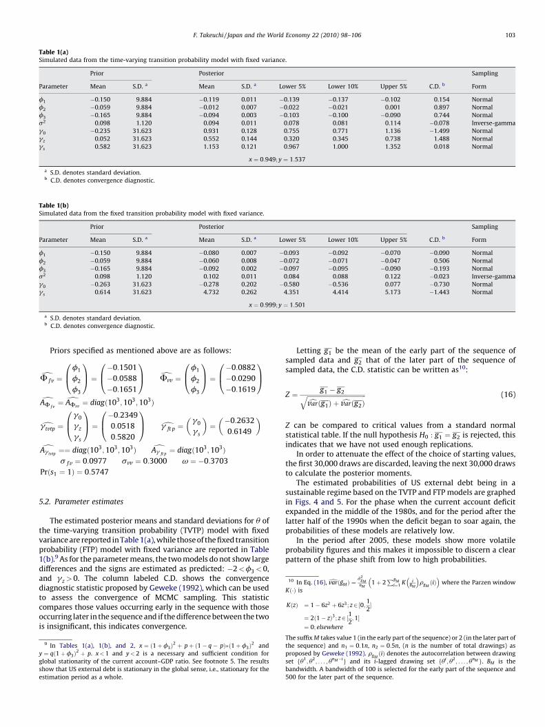
Table 1(a)Simulated data from the time-varying transition probability model with fixed variance.

Prior Posterior Sampling

Parameter Mean S.D. a Mean S.D. a Lower 5% Lower 10% Upper 5% C.D. b Form

f1 �0.150 9.884 �0.119 0.011 �0.139 �0.137 �0.102 0.154 Normal

f2 �0.059 9.884 �0.012 0.007 �0.022 �0.021 0.001 0.897 Normal

f3 �0.165 9.884 �0.094 0.003 �0.103 �0.100 �0.090 0.744 Normal

s2 0.098 1.120 0.094 0.011 0.078 0.081 0.114 �0.078 Inverse-gamma

g0 �0.235 31.623 0.931 0.128 0.755 0.771 1.136 �1.499 Normal

gz 0.052 31.623 0.552 0.144 0.320 0.345 0.738 1.488 Normal

gs 0.582 31.623 1.153 0.121 0.967 1.000 1.352 0.018 Normal

x ¼ 0:949; y ¼ 1:537

a S.D. denotes standard deviation.b C.D. denotes convergence diagnostic.

Table 1(b)Simulated data from the fixed transition probability model with fixed variance.

Prior Posterior Sampling

Parameter Mean S.D. a Mean S.D. a Lower 5% Lower 10% Upper 5% C.D. b Form

f1 �0.150 9.884 �0.080 0.007 �0.093 �0.092 �0.070 �0.090 Normal

f2 �0.059 9.884 �0.060 0.008 �0.072 �0.071 �0.047 0.506 Normal

f3 �0.165 9.884 �0.092 0.002 �0.097 �0.095 �0.090 �0.193 Normal

s2 0.098 1.120 0.102 0.011 0.084 0.088 0.122 �0.023 Inverse-gamma

g0 �0.263 31.623 �0.278 0.202 �0.580 �0.536 0.077 �0.730 Normal

gs 0.614 31.623 4.732 0.262 4.351 4.414 5.173 �1.443 Normal

x ¼ 0:999; y ¼ 1:501

a S.D. denotes standard deviation.b C.D. denotes convergence diagnostic.

10 In Eq. (16), dvarðgMÞ ¼s2

gMnM

1þ 2PBM

i¼1 K iBM

� �rgMðiÞ

� �where the Parzen window

Kð�Þ is

KðzÞ ¼ 1� 6z2 þ 6z3; z2 ½0;12�

¼ 2ð1� zÞ3; z2 ½12;1�

¼ 0; elsewhere

F. Takeuchi / Japan and the World Economy 22 (2010) 98–106 103

Priors specified as mentioned above are as follows:

dF fv ¼f1

f2

f3

0B@1CA ¼ �0:1501

�0:0588

�0:1651

0B@1CA dFvv ¼

f1

f2

f3

0B@1CA ¼ �0:0882

�0:0290

�0:1619

0B@1CA

dAF fv¼ dAFvv

¼ diagð103;103;103Þ

dg tvtp ¼g0

gz

gs

0B@1CA ¼ �0:2349

0:0518

0:5820

0B@1CA dg ft p ¼

g0

gs

� �¼�0:2632

0:6149

� �dAgtvtp

¼¼ diagð103;103;103Þ dAg ft p¼ diagð103;103Þ

s f v ¼ 0:0977 svv ¼ 0:3000 v ¼ �0:3703

Prðs1 ¼ 1Þ ¼ 0:5747

5.2. Parameter estimates

The estimated posterior means and standard deviations for u ofthe time-varying transition probability (TVTP) model with fixedvariance are reported in Table 1(a), while those of the fixed transitionprobability (FTP) model with fixed variance are reported in Table1(b).9 As for the parameter means, the two models do not show largedifferences and the signs are estimated as predicted: �2<f3 <0,and gz >0. The column labeled C.D. shows the convergencediagnostic statistic proposed by Geweke (1992), which can be usedto assess the convergence of MCMC sampling. This statisticcompares those values occurring early in the sequence with thoseoccurring later in the sequence and if the difference between the twois insignificant, this indicates convergence.

9 In Tables 1(a), 1(b), and 2, x ¼ ð1þ f3Þ2 þ pþ ð1� q� pÞ�ð1þ f3Þ

2 and

y ¼ qð1þ f3Þ2 þ p. x<1 and y<2 is a necessary and sufficient condition for

global stationarity of the current account–GDP ratio. See footnote 5. The results

show that US external debt is stationary in the global sense, i.e., stationary for the

estimation period as a whole.

Letting g1 be the mean of the early part of the sequence ofsampled data and g2 that of the later part of the sequence ofsampled data, the C.D. statistic can be written as10:

Z ¼ g1 � g2ffiffiffiffiffiffiffiffiffiffiffiffiffiffiffiffiffiffiffiffiffiffiffiffiffiffiffiffiffiffiffiffiffiffiffiffifficvarðg1Þ þ cvarðg2Þq (16)

Z can be compared to critical values from a standard normalstatistical table. If the null hypothesis H0 : g1 ¼ g2 is rejected, thisindicates that we have not used enough replications.

In order to attenuate the effect of the choice of starting values,the first 30,000 draws are discarded, leaving the next 30,000 drawsto calculate the posterior moments.

The estimated probabilities of US external debt being in asustainable regime based on the TVTP and FTP models are graphedin Figs. 4 and 5. For the phase when the current account deficitexpanded in the middle of the 1980s, and for the period after thelatter half of the 1990s when the deficit began to soar again, theprobabilities of these models are relatively low.

In the period after 2005, these models show more volatileprobability figures and this makes it impossible to discern a clearpattern of the phase shift from low to high probabilities.

The suffix M takes value 1 (in the early part of the sequence) or 2 (in the later part of

the sequence) and n1 ¼ 0:1n, n2 ¼ 0:5n, (n is the number of total drawings) as

proposed by Geweke (1992). rgMðiÞ denotes the autocorrelation between drawing

set fu1; u2

; . . . ; unM�ig and its i-lagged drawing set fui; u2

; . . . ; unM g. BM is the

bandwidth. A bandwidth of 100 is selected for the early part of the sequence and

500 for the later part of the sequence.

Fig. 4. The probability of US external debit being stationary (sustainable), results of the TVTP (fixed variance) model.

Fig. 5. The probability of US external debit being stationary (sustainable), results of the FTP model.

Fig. 6. The probability of US external debit being stationary (sustainable), results of the TVTP (time-varying variance) model.

F. Takeuchi / Japan and the World Economy 22 (2010) 98–106104

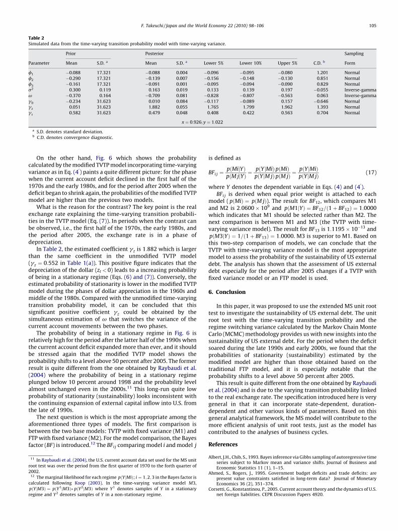
Table 2Simulated data from the time-varying transition probability model with time-varying variance.

Prior Posterior Sampling

Parameter Mean S.D. a Mean S.D. a Lower 5% Lower 10% Upper 5% C.D. b Form

f1 �0.088 17.321 �0.088 0.004 �0.096 �0.095 �0.080 1.201 Normal

f2 �0.290 17.321 �0.139 0.007 �0.156 �0.148 �0.130 0.851 Normal

f3 �0.161 17.321 �0.091 0.001 �0.095 �0.094 �0.090 0.829 Normal

s2 0.300 0.119 0.163 0.019 0.133 0.139 0.197 �0.055 Inverse-gamma

v �0.370 0.164 �0.709 0.081 �0.828 �0.807 �0.563 0.063 Inverse-gamma

g0 �0.234 31.623 0.010 0.084 �0.117 �0.089 0.157 �0.646 Normal

gz 0.051 31.623 1.882 0.055 1.765 1.799 1.962 1.393 Normal

gs 0.582 31.623 0.479 0.048 0.408 0.422 0.563 0.704 Normal

x ¼ 0:926; y ¼ 1:022

a S.D. denotes standard deviation.b C.D. denotes convergence diagnostic.

F. Takeuchi / Japan and the World Economy 22 (2010) 98–106 105

On the other hand, Fig. 6 which shows the probabilitycalculated by the modified TVTP model incorporating time-varyingvariance as in Eq. (4

0) paints a quite different picture: for the phase

when the current account deficit declined in the first half of the1970s and the early 1980s, and for the period after 2005 when thedeficit began to shrink again, the probabilities of the modified TVTPmodel are higher than the previous two models.

What is the reason for the contrast? The key point is the realexchange rate explaining the time-varying transition probabili-ties in the TVTP model (Eq. (7)). In periods when the contrast canbe observed, i.e., the first half of the 1970s, the early 1980s, andthe period after 2005, the exchange rate is in a phase ofdepreciation.

In Table 2, the estimated coefficient gz is 1:882 which is largerthan the same coefficient in the unmodified TVTP model(gz ¼ 0:552 in Table 1(a)). This positive figure indicates that thedepreciation of the dollar (zt <0) leads to a increasing probabilityof being in a stationary regime (Eqs. (6) and (7)). Conversely, theestimated probability of stationarity is lower in the modified TVTPmodel during the phases of dollar appreciation in the 1960s andmiddle of the 1980s. Compared with the unmodified time-varyingtransition probability model, it can be concluded that thissignificant positive coefficient gz could be obtained by thesimultaneous estimation of v that switches the variance of thecurrent account movements between the two phases.

The probability of being in a stationary regime in Fig. 6 isrelatively high for the period after the latter half of the 1990s whenthe current account deficit expanded more than ever, and it shouldbe stressed again that the modified TVTP model shows theprobability shifts to a level above 50 percent after 2005. The formerresult is quite different from the one obtained by Raybaudi et al.(2004) where the probability of being in a stationary regimeplunged below 10 percent around 1998 and the probability levelalmost unchanged even in the 2000s.11 This long-run quite lowprobability of stationarity (sustainability) looks inconsistent withthe continuing expansion of external capital inflow into U.S. fromthe late of 1990s.

The next question is which is the most appropriate among theaforementioned three types of models. The first comparison isbetween the two base models: TVTP with fixed variance (M1) andFTP with fixed variance (M2). For the model comparison, the Bayesfactor (BF) is introduced.12 The BFi j comparing model i and model j

11 In Raybaudi et al. (2004), the U.S. current account data set used for the MS unit

root test was over the period from the first quarter of 1970 to the forth quarter of

2002.12 The marginal likelihood for each regime pðYjMiÞ; i ¼ 1;2;3 in the Bayes factor is

calculated following Koop (2003). In the time-varying variance model M3,

pðY jM3Þ ¼ pðY1jM3Þ� pðY2jM3Þ where Y1 denotes samples of Y in a stationary

regime and Y2 denotes samples of Y in a non-stationary regime.

is defined as

BFi j ¼pðMijYÞpðM jjYÞ ¼

pðY jMiÞpðMiÞpðYjM jÞpðM jÞ ¼

pðY jMiÞpðY jM jÞ (17)

where Y denotes the dependent variable in Eqs. (4) and (40).

BFi j is derived when equal prior weight is attached to eachmodel ( pðMiÞ ¼ pðM jÞ). The result for BF12, which compares M1and M2 is 2:0600 109 and pðM1jYÞ ¼ BF12=ð1þ BF12Þ ¼ 1:0000which indicates that M1 should be selected rather than M2. Thenext comparison is between M1 and M3 (the TVTP with time-varying variance model). The result for BF13 is 1:1195 10�13 andpðM3jYÞ ¼ 1=ð1þ BF13Þ ¼ 1:0000. M3 is superior to M1. Based onthis two-step comparison of models, we can conclude that theTVTP with time-varying variance model is the most appropriatemodel to assess the probability of the sustainability of US externaldebt. The analysis has shown that the assessment of US externaldebt especially for the period after 2005 changes if a TVTP withfixed variance model or an FTP model is used.

6. Conclusion

In this paper, it was proposed to use the extended MS unit roottest to investigate the sustainability of US external debt. The unitroot test with the time-varying transition probability and theregime switching variance calculated by the Markov Chain MonteCarlo (MCMC) methodology provides us with new insights into thesustainability of US external debt. For the period when the deficitsoared during the late 1990s and early 2000s, we found that theprobabilities of stationarity (sustainability) estimated by themodified model are higher than those obtained based on thetraditional FTP model, and it is especially notable that theprobability shifts to a level above 50 percent after 2005.

This result is quite different from the one obtained by Raybaudiet al. (2004) and is due to the varying transition probability linkedto the real exchange rate. The specification introduced here is verygeneral in that it can incorporate state-dependent, duration-dependent and other various kinds of parameters. Based on thisgeneral analytical framework, the MS model will contribute to themore efficient analysis of unit root tests, just as the model hascontributed to the analyses of business cycles.

References

Albert, J.H., Chib, S., 1993. Bayes inference via Gibbs sampling of autoregressive timeseries subject to Markov mean and variance shifts. Journal of Business andEconomic Statistics 11 (1), 1–15.

Ahmed, S., Rogers, J., 1995. Government budget deficits and trade deficits: arepresent value constraints satisfied in long-term data? Journal of MonetaryEconomics 36 (2), 351–374.

Corsetti, G., Konstantinou, P., 2005. Current account theory and the dynamics of U.S.net foreign liabilities. CEPR Discussion Papers 4920.

F. Takeuchi / Japan and the World Economy 22 (2010) 98–106106

Filardo, A.J., Gordon, S.F., 1998. Business cycle durations. Journal of Econometrics 85(1), 99–123.

Francq, C., Zakoıan, J., 2001. Stationarity of multivariate Markov-switching ARMAmodels. Journal of Econometrics 102 (2), 339–364.

Geweke, J., 1992. Evaluating the accuracy of sampling-based approaches to thecalculation of posterior moments. In: Bernardo, J.M.,Berger, J.O.,David, A.P.,Smith,A.F.M. (Eds.),Bayesian Statistics 4. Oxford University Press, Oxford, pp. 169–194.

Hall, S., Psaradakis, Z., Sola, M., 1999. Detecting periodically collapsing bubbles: aMarkov-switching unit root test. Journal of Applied Econometrics 14 (2), 143–154.

Hamilton, J.D., 1994. Time Series Analysis. Princeton University Press, Princeton.Higgins, M., Klitgaard, T., Tille, C., 2005. The income implications of rising U.S.

international liabilities. Current Issues in Economics and Finance 11 (2). FederalReserve Bank of New York.

IMF, 2005. Globalization and external imbalances. World Economic Outlook (April),109–156.

Koop, G., 2003. Bayesian Econometrics. Wiley, Chichester.Matsubayashi, Y., 2005. Are US current account deficits unsustainable? Testing for

the private and government intertemporal budget constraints. Japan and theWorld Economy 17 (2), 223–237.

Nelson, C., Zivot, E., Piger, J., 2001. Markov regime switching and unit root tests.Federal Reserve Bank of St. Louis Working Paper 2001-013A.

Obstfeld, M., Rogoff, K., 2004. The unsustainable US current account positionrevisited. NBER Working Paper Series 10869.

Ogawa, E., Kudo, T., 2004. How much depreciation of the US dollar for sustainabilityof the current accounts? Hitotsubashi University, Hi-Stat Discussion PaperSeries 44.

Perron, P., 1997. Further evidence on breaking trend functions in macroeconomicvariables. Journal of Econometrics 80 (2), 355–385.

Raybaudi, M., Sola, M., Spagnolo, F., 2004. Red signals: Current account deficits andsustainability. Economics Letters 84, 217–223.

Trehan, B., Walsh, C., 1988. Common trends, the government’s budget constraint,and revenue smoothing. Journal of Economic Dynamics and Control 12 (2–3),425–444.

Trehan, B., Walsh, C., 1991. Testing intertemporal budget constraints: Theory andapplications to U.S. federal budget and current account deficits. Journal ofMoney, Credit and Banking 23 (2), 206–223.

Webber, A.G., 2000. Newton’s gravity law and import prices in the Asia Pacific. Japanand the World Economy 12 (1), 71–87.