us army armament research ai … 02532 c. 3a!^-_..j v ad technical report arbrl-tr-02532...
TRANSCRIPT

BRL02532c. 3A
! - _..JV
AD
TECHNICAL REPORT ARBRL-TR-02532
N A V I E R - S T O K E S C O M P U T A T I O N S O F P R O J E C T I L E
B A S E FLOW A T T R A N S O N I C S P E E D S W I T H A N D
W I T H O U T B A S E I N J E C T I O N
Jubaraj SahuCharles J. Nietubicz
J. L. Steger
November 1983BLC2. 32
US ARMY ARMAMENT RESEARCH Ai DEVELOPMENT CENTERBALLISTIC RESEARCH LABORATORY
ABERDEEN PROVING GROUND, MARYLAND
Approved for public release; distribution unlimited.

Destroy this report when it is no longer needed.Do not return it to the originator.
Additional copies of this report may be obtainedfrom the National Technical Information Service,U. S. Department of Commerce, Springfield, Virginia22161.
The findings in this report are not to be construed asan official Department of the Army position, unlessso designated by other authorized documents.
Tlie uae of trade names or m.v.ufaaturers' names in this reportdoes not constitute indorsement of any aonmeroial product.

UNCLASSIFIEDSECURITY CLASSIFICATION OF THIS PAGE (When Data Entered)
REPORT DOCUMENTATION PAGE READ INSTRUCTIONSBEFORE COMPLETING FORM
t. REPORT NUMBER
TECHNICAL REPORT ARBRL-TR-02532
2. GOVT ACCESSION NO. 3. RECIPIENT'S CATALOG NUMBER
4. TITLE (and Subtitle)
NAVIER-STOKES COMPUTATIONS OF PROJECTILE BASEFLOW AT TRANSONIC SPEEDS WITH AND WITHOUT BASEINJECTION
5. TYPE OF REPORT 4 PERIOD COVERED
Final6. PERFORMING ORG. REPORT NUMBER
7. AUTHORO) 8. CONTRACT OR GRANT NUMBER(s)
J. Sahu, C. J. Nietubicz, & J. L. Steger*
9. PERFORMING ORGANIZATION NAME AND ADDRESS
U.S. Army Ballistic Research Laboratory, ARDCATTN: DRDAR-BLL(A)
Abfrdpen Proving firnunH. MarylanH ?1flflR
10. PROGRAM ELEMENT. PROJECT, TASKAREA a WORK UNIT NUMBERS
RDT&E 1L161102AH43
11. CONTROLLING OFFICE NAME AND ADDRESS
US Army AMCCOM, ARDCBallistic Research Laboratory, ATTN: DRSMC-BLA-S(AAberdeen Proving Ground. MD 21005
12. REPORT DATE
November 198313- NUMBER OF PAGES
39U. MONITORING AGENCf NAME ft ADDRESSflf different from Controlling Office) 15. SECURITY CLASS, (of thlm report)
UNCLASSIFIEDI5«. DECLASSIFICATION/ DOWNGRADING
SCHEDULE
16. DISTRIBUTION STATEMENT (of this Report)
Approved for public release; distribution unlimited.
17. DISTRIBUTION STATEMENT fof (ha abstract entered In Block 30, II different from Report)
18. SUPPLEMENTARY NOTES
*Stanford UniversityDepartment of Aeronautics and AstronauticsATTN: Prof. J. L. StegerStanford, CA 94305-Jicmiufu, in ^M-JU?
9. KEY WORDS (Continue on reverae aide It naceaaary and Identify by block number)
BLOG. 305
Base FlowTransonic SpeedsBase BleedProjectile Aerodynamics
Navier-Stokes ComputationsBase PressureDrag Components
Computational Fluid Dynamics20. ABSTRACTYOnrttnue em r»v»ri» afOa ft n+cMaary ami Identify by block number)
A computational capability has been developed for predicting the flowfield about the entire projectile, including the recirculatory base flow, attransonic speeds. Additionally, the computer code allows mass injection atthe projectile base and hence is used to show the effects of base bleed onbase drag. Computations have been made for a secant-ogive-cylinder projectilefor a series of Mach numbers in the transonic flow regime. Computed resultsshow the qualitative and quantitative nature of base flow with and without
on FORM*'•' 1 JAN 73 EDITION OF » NOV 65 IS OBSOLETE UNCLASSIFIED
SECUWTY CLASSIFICATION OF THIS PAGE fWwn Data Entered)

UNCLASSIFIEDSECURITY CLASSIFICATION Of THIS PAQgfWien Dmte Bntftwt)
20. ABSTRACT (Continued)
base bleed. The reduction in base drag with base bleed is clearly predicted forvarious mass injection rates and for Mach numbers .9 < M < 1.2. The encouragingresults obtained indicate that this computational technique may provide usefuldesign guidance for shell with base bleed.
UNCLASSIFIEDSECURITY CLASSIFICATION OF THIS PAGEflWien Data Entered)

TABLE OF CONTENTS
Page
LIST OF ILLUSTRATIONS 5
I. INTRODUCTION 7
II. PHYSICAL PROBLEM 9
III. GOVERNING EQUATIONS 9
IV. NUMERICAL METHOD 12
A. Computational Algorithm.... 12
B. Finite Difference Equations 13
C. Flow Field Segmentation ' 13
D. Implementation of Boundary Conditions 13
1. Base Flow without Base Injection 13
2. Base Flow with Base Injection 15
E. Computational Grid 16
V. RESULTS 17
VI. SUMMARY 19
REFERENCES .' 31
LIST OF SYMBOLS 33
DISTRIBUTION LIST 37

This page Left Intentionally Blank
LIST OF ILLUSTRATIONS
Figure Page
1 Schematic Illustration of Base Region Flow Field with Base81 eed 20
2 Schematic Illustration of Flow Field Segmentation 21
3 Computational Grid for Flow Field Computations 22
4 Expanded Grid in the Vicinity of the Projectile 22
5 Grid Adapted to the Shear Layer 23
6 Model Geometry 23
7 Longitudinal Surface Pressure Distribution, M = 0.9, a = 0,Ij = 0 (without Base Bleed) 24
8 Longitudinal Surface Pressure Distribution, M = 0.9, a = 0,Ij = .13 (with Base Bleed) 24
9 Velocity Vector Field, M = 0.9, a = 0, Ij = 0 25
10 Velocity Vector Field, M = 0.9, a = 0, Ij = .01 25
11 Velocity Vector Field, M = 0.9, a = 0, Ij = .07 26
12 Velocity Vector Field, M = 0.9, a = 0, Ij = .13 26
13 Stream Function Contours, M = 0.9, a = 0, Ij = 0 27
14 Stream Function Contours, M = 0.9, a = 0, Ij = .01 27
15 Stream Function Contours, M = 0.9, a = 0, Ij = .07 28
16 Stream Function Contours, M = 0.9, a = 0, Ij = .13 28
17 Variation of Base Drag Coefficient with Base Bleed, M = 0.9,ot = 0 29
18 Variation of Total Drag Coefficient with Base Bleed, M = 0.9,a= 0 29
19 Variation of Base Drag Coefficient with Mach Number, a = 0(with and without Base Bleed) 30
20 Variation of Total Drag Coefficient with Mach Number, a = 0(with and without Base Bleed) 30

This page Left Intentionally Blank

I. INTRODUCTION
A major area of concern in shell design is the total aerodynamic drag..The designer, ever desirous of increasing the range and/or terminal velocityof projectiles, is eager to decrease the aerodynamic drag.
The total drag of projectiles can be divided into three components: (1)pressure drag (excluding the base region), (2) viscous (skin friction) drag,and (3) base drag. For a typical shell at M = .90 the relative magnitudes ofthe aerodynamic drag components are: (1) pressure drag, 20%, (2) viscousdrag, 30%, and (3) base drag, 50%. The pressure and viscous components gener-ally cannot be reduced significantly without adversely affecting the stabilityof shell. Recent attempts to reduce the total drag are therefore directed atreducing the base drag.
A number of studies have been made to examine the total drag reductiondue to the addition of a boattail. Although this is very effective in reduc-ing the total drag, it has a negative impact on the aerodynamic stability ofshell especially at transonic velocities. An excellent review of the effectof boattailing on total drag and base pressure is presented in Reference 1.
Another effective means of reducing the base drag is that of 'base bleed1
or 'base injection.1 In this method, a small amount of mass is injected intothe base region which increases the base pressure and thus reduces the basedrag. Recent range and precision tests2 of a 155mm projectile with and with-out base bleed have been conducted and an 85% reduction in base drag wasobtained. Presently the XM864 is an active projectile design which is attempt-ing to use the base bleed concept for increased range. This concept of massinjection at the projectile base has been widely studied for supersonic flowsand much of the work has been reported in Reference 3. One limited study at.supersonic speeds was made at BRL and the results were reported by Dickinson.**The supersonic regime has typically been the area where increased range due to
Sedney, R.f "Review of Ease Drag," Report No. 1337, U.S. Army BallisticResearch Laboratory, Aberdeen Proving Ground, Maryland, 21005, October1966 (AD 808767).
"155mm ERFB Base Bleed Range and Precision Tests, " Conducted at Proof andExperimental Test Establishment, Nicolet, Quebec, for Space ResearchCorporation, January 11, 1978.
Murthy, S.N.B. (Ed.), "Progress in Astronautics and Aeronautics: Aerody-namics of Base Combustion," Vol. 40, AIAA, New York, 1976.
Dickinson, E.R., "The Effectiveness of Base-Bleed in Reducing Drag ofBoattailed Bodies at Supersonic Velocities," Memorandum Report No. 1244, U.S.Army Ballistic Research Laboratory, Aberdeen Proving Ground, Maryland21005, 1960 (AD 234315).

drag reduction has been studied. Thus, only limited attention has been focus-sed on the 'base bleed1 problem in transonic flow. A limited study made inthe transonic flow regime has been reported in Reference 5 which describes theeffects of base bleed on various afterbody configurations.
Most of the work using the 'base bleed1 concept has been either experi-mental or semi-empirical in nature. Sophisticated numerical techniques havenot yet been utilized to predict the effects of base bleed on the base dragreduction. Limited computational work was reported recently by Sullins, etal.6 Their work dealt with the numerical computation of the base region flowof a supersonic combustion ramjet engine using two-dimensional Navier-Stokesequations. They computed the flow field in the vicinity of the base withparallel gas injection and established the effect of base injection on suchflows.
Because of the recent advances in computer technology, numerical computa-tional capabilities have been developed to predict the aerodynamic behavior ofartillery shell. Recent papers7'8 have reported the development and applica-tion of the Azimuthal-Invariant Thin-Layer Navier-Stokes computational techni-que to predict the flow about slender bodies of revolution at transonicspeeds. This technique has been modified for base flow analysis and theresulting new numerical capability9 is used here to predict the base pressureof shell at transonic speeds including the effect of base bleed. Computedresults show quantitative and qualitative details of the base flow structure.The technique computes the full flow field over the projectile at transonicspeeds; therefore, all three components of the total drag (pressure, viscous,and base drag) are computed. This computational technique is then applied topredict the effects of base bleed on the base drag reduction at transonic
5. Sykes, D.M., "Cylindrical and Boattailed Afterbodies in Transonic Flowwith Gas Ejection," AIAA Journal, Vol. 8, No. 3, March 1970, pp. 588-589.
6. Sulline, G.A., Anderson, J.D., and Drummond, J.P., "Numerical Investiga-tion of Supersonic Base Flow with Parallel Injection," AIAA Paper No. 82-1001, June 1982.
7. Nietubicz, C.J., Pulliam, T.H., and Steger, J.L., "Numerical Solution ofthe Azimuthal-Invariant Thin-Layer Navier-Stokes Equations," ARBRL-TR-02227, U.S. Army Ballistic Research Laboratory, Aberdeen Proving Ground,Maryland 21005, March 1980 (AD A085716).
8. Nietubicz, C.J., "Navier-Stokes Computations for Conventional and HollowProjectile Shapes at Transonic Velocities," ARBRL-MR-03184, U.S. ArmyBallistic Research Laboratory, Aberdeen Proving Ground, Maryland 21005,July 1982 (AD A116866).
9. Sahu, J., Nietubicz, C.J., and Steger, J.L., "Numerical Computation ofBase Flow for a Projectile at Transonic Speeds," ARBRL-TR-02495, U.S. ArmyBallistic Research Laboratory, Aberdeen Proving Ground, Maryland 21005,June 1983 (AD Al30293).
8
speeds. The combined effect of boattailing and base bleed is, however, notconsidered in this report.
Brief descriptions of the physical problem and the governing equationsare given in Sections II and III, respectively. The computational techniqueand the method of solution are discussed in Section IV. In Section V, resultsare shown for transonic base pressure computations for a 6-caliber secant-ogive-cylinder shape for .9 < M < 1.2, with and without base bleed. Velocityvector plots and stream function contour plots are presented to show the qual-itative features of the flow field in the base region. Quantitative compari-sons of base drag and the total drag, both with and without base injection,have been made. The encouraging results show that the present computationaltechnique can be used to study the effects of base bleed on base drag and thuscan have a positive impact on the XM864 devleopment. Although results in thisreport are presented for transonic speeds, current computational efforts aredirected at supersonic velocities.
II. PHYSICAL PROBLEM
The physical problem deals with the transonic flow over a projectile,including the base region. Although the entire projectile flow is computed,the emphasis is on the flow field in the base region of the projectile. Asmall amount of air is injected at the projectile base in the direction paral-lel to the primary flow. The injection at the base can be concentrated at thecenter of the base or spread throughout the entire base. In the present work,however, the injection takes place over 90% of the base. Figure 1 shows aschematic illustration of the base region flow field with base injection. Thedividing streamline separates the recirculary base flow from the primaryexternal flow. The flow field is dominated by separation and mixed regions oflocally supersonic and subsonic flows.
The complete set of time-dependent generalized axisymmetric thin-layerNavier-Stokes equations is solved to obtain a numerical solution to thisproblem. The numerical technique used is an implicit finite-differencescheme. Although time-dependent calculations are made, the transient flow isnot of primary interest at the present time. The steady flow is the desiredresult which is obtained in a time asymptotic fashion.
III. GOVERNING EQUATIONS
The Azimuthal Invariant (or Generalized Axisymmetric) thin-layer Navier-Stokes equations for general spatial coordinates £, n, i, can be written as7
where £ = 5(x,y,z,t) is the longitudinal coordinate
n = ri(y,z,t) is the circumferential coordinate

£ = 5(x,y,z,t) is the near normal coordinate
T = t is the timeA A A A
The vector of dependent variables q and the flux vectors E, G, H aregiven as
q = J-1
ppuPV
PW
e
G =
E = J
PUpull + £xp
PvU + £yp
pwU + SZP
(e + p) U - £ p
PW
puW + t, pA
pvW + c p
pwW + C p
(e + p) W
H =
pVR<j»n(V
0
0
£t) + F-n t)-
0
where J is the Jacobian of transformation.
The thin layer viscous terms valid for high Reynolds number flow areA
contained in the vector S, where
S =
A y
+ (n/3)(5xu
0
(u/3)(cxuc
.5M(U2 + V2 + W2)
10

The velocities
U =
V = nt + n u + n v + n w (2)L X jr i
w = c + cu + cv + cw
represent the contravariant velocity components.
The Cartesian velocity components (u, v, w) are nondimensionalized withrespect to a^ (the free stream speed of sound). The density (p) is referencedto p^ and total energy (e) to p a . The local pressure is determined usingthe equation of state,
P = (T - l)[e - 0.5p(u2 + v2 + w2)] (3)
where y is the ratio of specific heats.
In Equation (1) a thin-layer approximation is used and the restrictionsfor axi symmetric flow are imposed. The details can be found in References 8and 9 and are not discussed here. Equation (1) contains only two spatialderivatives; however, it retains all three momentum equations, thus allowing adegree of generality over the standard axisymmetric equations. In particular,the circumferential velocity is not assumed to be zero, thus allowing computa-tions for spinning projectiles or swirl flow to be accomplished. There issome evidence which indicates that base pressure can change due to the spin ofa projectile. Although the present work considers base flow with no spin,base flow with spin is of interest and can be studied using the presenttechnique.
For the computation of turbulent flows a turbulence model must be sup-plied. In the present calculations a Cebeci-type two layer algebraic eddyviscosity model as modified by Baldwin and Lomax10 is used. In their twolayer model the inner region follows the Prandtl-Van Driest formulation.Their outer formulation can be used in wakes as well as in attached and sepa-rated boundary layers. In both the inner and outer formulations the distribu-tion of vorticity is used to determine length scales, thereby avoiding thenecessity of finding the outer edge of the boundary layer (or wake). Themagnitude of the local vorticity for the axisymmetric formulation is given by
" I • ' > * * < - ) * * - > * ( 4 )
10. Baldwin, B.S., and Lomax, H., "Thin-Layer Approximation and AlgebraicModel for Separated Turbulent Flows," AIAA Paper No. 78-257, 1978.
11
In determining the outer length scale a function10
F(y) = y|«| [1 - exp(-y+/A+)] (5)
is used where y+ and A+ are the conventional boundary layer terms. For thebase flow (or wake flow) the exponential term of Equation (5) is set equal tozero.
IV. NUMERICAL METHOD
A. Computational Algorithm
An implicit, approximate factorization, finite-difference scheme in deltaform as described by Beam and Warming11 is used. An implicit method waschosen because it permits a time step much greater than that allowed by explic-it schemes. For problems in which the transient solution is of no interest,this offers the advantage of being able to reach the steady state solutionfaster than existing explicit schemes.
The Beam-Warming implicit algorithm has been used successfully in variousapplications.7"13 The algorithm can be first or second order accurate in timeand second or fourth order accurate in space. The equations are factored(spatially split) which reduces the solution process to one-dimensional prob-lems at a given time level. Central difference operators are employed andthe algorithm produces block tridiagonal systems for each space coordinate.The main computational work is contained in the solution of these block tri-diagonal systems of equations.
11. Beam, R., and Warming, R.F., "An Implicit Factored Scheme for theCompressible Navier-Stokes Equationsf" AIAA Journal, Vol. 16, No. 4,April 1978, pp. S93-402.
12. Steger, J.L., "Implicit Finite Difference Simulation of Flow AboutArbitrary Geometries with Application to Airfoils," AIAA Journal, Vol.16, No. 7, July 1978, pp. 679-686.
13. Pulliam, T.H., and Steger, J.L., "On Implicit Finite-Difference Simula-tions of Three-Dimensional Flow, " AIAA Journal, Vol. 18, No. 2, February1980, pp. 159-167.
12

B. Finite Difference Equations
The resulting finite difference equations, written in delta form are
(I + h6^An - ejj'1? A J)(I + ha^C11 - eIJ'1V A J
^J) (qn+1 - qn) = - A t ( 6 E n + 6Gn (6)
- AtHn -
Here h = At because only first order accuracy in the time differencing isneeded for the steady state flows considered here. This choice corresponds tothe Euler implicit time differencing. The 6's represent central differenceoperators, A and V are forward and backward difference operators,
A A
A -\C Jip
respectively. The Jacobian matrices A = —r, C = —- together with the coeffi-. . 3q 3q
cient matrix M obtained from the local time linearization of S are describedin detail in Reference 6. Fourth order explicit (ep) and implicit (e,) numer-ical dissipation terms are incorporated into the differencing scheme to damphigh frequency growth and thus to control the nonlinear instabilities. Atypical range for the smoothing coefficients is EE = (1 to 5) At withel = 3eE'
C. Flow Field Segmentation
Figure 2 is a schematic illustration of the flow field segmentation usedto compute the entire projectile flow field including the base flow. It showsthe transformation of the physical domain into the computational domain andthe details of the flow field segmentation procedure in both domains.
The cross hatched region represents the projectile. The line BC is theprojectile base and the region ABCD is the base region or the wake. The lineAB is a computational cut through the physical wake region which acts as arepetitive boundary in the computational domain. Implicit integration iscarried out in both £ and t, directions. (See Figure 2.) Note the presence ofthe lines BC (the base) and EF (nose axis) in the computational domain. Theyboth, however, act as boundaries in the computational domain and special caremust be taken in forming the block tridiagonal matrix in the C direction. Thedetails are presented in the next section.
D. Implementation of Boundary Conditions
1. Base Flow without Base Injection.
The no-slip boundary conditions for viscous flow are enforced bysetting
13

U = V = W = 0 (7)
on the projectile surface except for the base. At the projectile base thevelocity component normal to the base is set to zero, i.e., U = 0, while otherflow variables are set equal to those at grid point next to the base.
Along the computational cut (line AB), the flow variables above andbelow the cut were simply averaged to determine the boundary conditions on thecut. On the centerline of the wake region, a symmetry condition is imposed:
w = 0(8)
Free stream conditions are used at the outer boundary. First orderextrapolation for all flow variables is used at the downstream boundary (linesAD and AG). During transient calculations, use of a specified outflow pres-sure can give rise to numericalEventually, these grow and swampsimply extrapolating pressure todure always used with supersonicsymmetry is used on the nose axis
oscillations in the base region flow field,the solution. This difficulty is avoided bythe downstream boundary which is the proce-outflow. A combination of extrapolation and(line EF).
As a result of the flow field segmentation procedure describedearlier, the block tridiagonal matrix in the 5 direction has elements at J =JB, JB+1 which are treated as internal boundaries in the computational domain.(J = JB represents the projectile base and J = JB+1 is the nose axis.) Theblock tridiagonal matrix in the 5 direction takes the following form (aftersetting e, = 0 to simplify the illustration)
14

I A3
-A2 I A4
'AJB-2 l AJB
0 I 0
0 1 0
-AJB+1 ? AJB+3
~AJMAX-2 l
AqJB+l
HjMAX-1
RHS
0
0
RHSJMAX-1
(9)
Here A's denote the quantity A and I is a 5x5 identity matrix. Note the
appearance of two uncoupled block tridiagonals. The rows at JB and JB+1 areparticularly simple because boundary conditions are updated explicitly at theend of inversions. These changes were easily implemented in a modular fashioninto an existing code for projectile base flow computations. One simply fillsthe block tridiagonal matrix ignoring the base JB and the nose axis JB+1.Elements in these rows are then overloaded as shown above. The flow fieldsegmentation does not affect the block tridiagonal matrix in the t, direction.
2. Base Flow with Base Injection.
The boundary conditions used for base flow with mass addition arepresented here. The boundary conditions along the projectile surface, at thecut and downstream boundary all remain the same as previously described.Along the base boundary the following conditions are imposed:
u =
v - Vj - 0
w = Wj = wjg_i (grid point next to the base)
p = pj = pst
BLOB. 3tt5The stagnation density is obtained from the following relation.
15
The amount of air injected into the base region can be specified by the massflow rate, m.. Since p- and Aj are known, Uj can be calculated for any givenmass flow rate. Rather than specifying m.,however, it is customary to specify
J .a mass injection parameter, Ij where Ij - Mi/P^uJ^' Most of the results withbase bleed are presented in terms of this parameter in the next section. Itis important to remember that the smaller the mass injection parameter, thesmaller is the amount of mass injected at the base.
E. Computational Grid
The finite difference grid used for the numerical computations wasobtained from a grid generator developed and reported in Reference 14. Thisprogram allows arbitrary grid point clustering, thus enabling grid points forthe projectile shapes to be clustered in the vicinity of the body surface.The grid consists of 108 points in the longitudinal direction and 50 points inthe radial direction. The full grid is shown in Figure 3 while Figure 4 showsan expanded view of the grid in the vicinity of the projectile. The computa-tional domain extended to 4 body lengths in front, 4 body lengths in theradial direction and 4 body lengths behind the base of the projectile. Thegrid points in the normal direction were exponentially stretched away from thesurface with the minimum spacing at the wall of .000020. This spacing locatesat least two points within the laminar sublayer.
The grid shown in Figure 4 was generated in two segments. First, thegrid in the outer region is obtained using an elliptic solver11* for the ogiveportion and straight-line rays for the remaining portion which runs all theway to downstream boundary. Second, the grid in the base region is obtainedsimply by extending the straight lines perpendicular to line AB down to thecenter line of symmetry (line CO). An exponential stretching with the minimumspacing of .000020 at line AB is used. It should be noted that the same mini-mum spacing .000020 is specified on both sides of the cut thus maintaining asmooth variation of grid across the cut. This spacing could, of course, beincreased downstream of the base. The number of grid points above and belowline AB is the same (50 points). As can be seen in Figure 4, the grid pointsare clustered near the nose-cylinder junction and at the projectile base whereappreciable changes in flow variables are expected.
As indicated in Figure 4, the fine viscous grid follows the cut labeledas AB in Figure 2. Insofar as the viscous shear layer begins to neck-downshortly behind the base, much of this fine grid resolution is wasted. As a
14. Steger, J.L., Nietubics, C.J., and Heavey, K.R., "A General CurvilinearGrid Generation Program for Projectile Configurations," ARBRL-MR-03142,U.S. Army Ballistic Research Laboratory, Aberdeen Proving Ground,Maryland 21005, October 1981 (AD A107334).
16

I(«2 Uj L> 2 Z J l + eD/2
consequence, logic has been implemented to adjust the grid cut AB to theviscous shear layer. Such a grid is shown in Figure 5 in which the height ofthe cut is determined from a moment of shear subject to various constraintsand averaging. Specifically, the cut height, "z, at each J-location is deter-mined by the relation
Z0
where the summation is carried out only for those points within an interval.20 < ZJL < D/2. Here D is the base diameter, «z is a central differenceoperator and e is a positive parameter which ensures a standard grid if all6 Uj. are zero or if e is very large. . Additional averaging is used in the x-direction (longitudinal direction). Preliminary results have been obtainedusing the grid shown in Figure 5 and further computations are underway.
V. RESULTS
The model geometry used in the present study is shown in Figure 6. Itconsists of a 3 caliber secant-ogive nose and a 3 caliber cylinder.
The free stream Reynolds number for the series of computations was fixedat 4.5 x io6 based on the total model leagth. The computations were startedfrom free stream conditions and marched in time to. obtain the steady statesolution. The initial calculation was made for M = 0.9. Previously convergedsolutions were then used as starting conditions for additional Mach numberruns to achieve faster convergence. The results are now presented for both(i) base flow without injection and (ii) base flow with injection.
Figures 7 and 8 show the distribution of the surface pressure coeffi-cient, Cp as a function of axial position without and with mass injection atthe base, respectively. The value of Cp beyond X/D = 6 is the value of pres-sure coefficient along the line extending from the cylinder portion straightto the downstream boundary. When there is no mass injection at the base thepressure distribution in Figure 7 reflects the shock pattern that typicallyoccurs on shell at transonic velocities, the rapid expansion which occurs atthe blunt base and the recompression that occurs downstream of the base. Thepressure coefficient distribution for a case with large mass addition is shownin Figure 8. The previously observed rapid expansion at the base and recom-pression downstream of it are seen to be virtually eliminated.
Figure 9 shows the velocity vector field in the base region for M = 0.9,a = 0 and I,• = 0. Each vector shows the magnitude and the direction of the
\)
velocity at that point. The figure shows the velocity field when there is nobase bleed and the recirculatory flow in the base region is clearly evident.
17
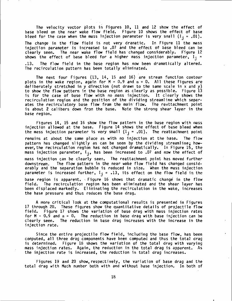
The velocity vector plots in Figures 10, 11 and 12 show the effect ofbase bleed on the near wake flow field. Figure 10 shows the effect of basebleed for the case when the mass injection parameter is very small (Ij = .01).The change in the flow field is not very dramatic. In Figure 11 the massinjection parameter is increased to .07 and the effect of base bleed can beclearly seen. The near wake flow field has changed considerably. Figure 12shows the effect of base bleed for a higher mass injection parameter, Ij =.13. The flow field in the base region has now been dramatically altered.The recirculation pattern has been totally eliminated.
The next four Figures (13, 14, 15 and 16) are stream function contourplots in the wake region, again for M = 0.9 and a = 0. All these figures aredeliberately stretched in y direction (not drawn to the same scale in x and y)to show the flow pattern in the base region as clearly as possible. Figure 13is for the case of base flow with no mass injection. It clearly shows therecirculation region and the position of the dividing streamline which separ-ates the recirculatory base flow from the main flow. The reattachment pointis about 2 calibers down from the base. Note the strong shear layer in thebase region.
Figures 14, 15 and 16 show the flow pattern in the base region with massinjection allowed at the base. Figure 14 shows the effect of base bleed whenthe mass injection parameter is very small (Ij = .01). The reattachment pointremains at about the same place as with no injection at the base. The flowpattern has changed slightly as can be seen by the dividing streamline; how-ever, the recirculation region has not changed dramatically. In Figure 15, themass injection parameter, Ij, has been increased to .07 and now the effect ofmass injection can be clearly seen. The reattachment point has moved furtherdownstream. The flow pattern in the near wake flow field has changed consid-erably and the separation bubble is reduced in size. When the mass injectionparameter is increased further, Ij = .13, its effect on the flow field in thebase region is apparent. Figure 16 shows that dramatic change in the flowfield. The recirculation region has been eliminated and the shear layer hasbeen displaced markedly. Eliminating the recirculation in the wake, increasesthe base pressure and thus reduces the base drag.
A more critical look at the computational results is presented in Figures17 through 20. These figures show the quantitative details of projectile flowfield. Figure 17 shows the variation of base drag with mass injection ratesfor M = 0.9 and a = 0. The reduction in base drag with base injection can beclearly seen. The reduction in base drag increases with the increase in theinjection rate.
Since the entire projectile flow field, including the base flow, has beencomputed, all three drag components have been computed and thus the total dragis determined. Figure 18 shows the variation of the total drag with varyingmass injection rates. Again, the reduction in the total drag is apparent. Asthe injection rate is increased, the reduction in total drag increases.
Figures 19 and 20 show, respectively, the variation of base drag and thetotal drag with Mach number both with and without base injection. In both of
18

these figures the computational results without base injection are shown bythe solid line whereas the dotted line represent the computational resultsobtained with injection. The reduction in base drag and thus total drag dueto base injection can be clearly seen. Figure 19 indicates that the reductionin base drag has increased with an increase in Mach number from .9 to .98while from M = 1.0 to 1.2, the drag reduction is apparently constant. In bothof the figures, the expected drag rise in the transonic speed regime is wellpredicted for .9 < M < 1.2 and the reduction in base drag and the total drag,due to base bleed has been clearly demonstrated.
VI. SUMMARY
A promising computational capability has been developed which computesthe full projectile flow field, including the recirculatory base flow, attransonic speeds both with and without base injection.
Numerical computations have been made for Mach numbers .9 < M < 1.2 topredict the base drag and the total drag with and. without base bleed. Compu-ted results show the qualitative features of the flow field in the near wakefor both cases. The effect of base injection on the qualitative nature ofbase flow has been clearly shown. Quantitative comparisons of base drag andthe total drag both with and without base injection have been made with eachother. For M = 0.9 and a = 0 the computational results show the reduction inbase drag and the total drag for several mass injection parameters. Resultsare also presented for .9 < M < 1.2 for a given mass injection rate and thereduction in base drag and the total drag has been demonstrated for this rangeof transonic speeds.
Current efforts are directed at the numerical computation of base flow atsupersonic speeds. The encouraging results obtained thus far at transonicspeeds indicate that the computational technique shows the promise of predict-ing the base drag and hence the total drag both with and without base injec-tion. Future computational efforts will investigate the combined effect ofboattailing and base bleed on the total aerodynamic drag.
19

M.
BASE BLEED
DIVIDING STREAMLINE
RECIRCULATION
REATTACHMENT POINT
Figure 1. Schematic Illustration of Base Region Flow Field with Base Bleed
20

X F
L.
O
3O
B CUT
PROJECTILE /S
E C
PHYSICAL DOMAIN
*. y . « . « ). z - ' )
x. y. z. t)
T-- t
COMPUTATIONAL DOMAIN
C F
:: I
o
o
' / s s / s s sA B E BODY
LOWER CUT- r— »> J, £
B AUPPER CUT
Figure 2. Schematic Illustration of Flow Field Segmentation
21

40-i
30-
20-
Y/D
10-
0-
— I i r IT i I i i I i i i i I i I T T I i i T TII I r V 't
-30 -20 -10 0 10 20 30
X/D
Figure 3. Computational Grid for Flow Field Computations
Y/D 3-
-2
X/D
Figure 4. .Expanded Grid in the Vicinity of the Projectile
22

2.0 -,
Y/D
05 6
Figure 5. Grid Adapted to the Shear Layer
18.315
ALL DIMENSIONS IN CALIBERS
Figure 6. Model Geometry
23

0.4-g
Figure 7. Longitudinal Surface Pressure Distribution,M = 0.9, a = 0, I • = 0 (without Base Bleed)
\j
0.4^
-0.4-
Figure 8. Longitudinal Surface Pressure Distribution,M = 0.9, o = 0 , Ij = ,13 (with Base Bleed)
24

I I
I I
Illllllllf IHM
lMf ffftft
f m if M
inn I///M
MM
,,in///////////////,,,,,,.
' 4
' • - • .tit***--*</
» » »4
4 4
t i
4
;~
"-
*-
»-
*'x
«
>
•
3 ssiiii i i i t
I
00O>
*X
OO•oo
o0C
N
O
OIIOII"O"oiOOl
OO3Ol
f inn f m
ntiM
MM
.,,
lit!!!/////////,t
t t
t t
}
t t
t f
f f
f .
'«
»»
»!
»
5 ; ;
2
S
-<> oIIaA
o00
„O
=
x ^•
rv iZL
.O4->O
•O
OO
Q*v
O6<Nc>
ooo.-Ho;
in

1.00
0.75
Y/D0.50
0.25
5 6 7 x/() 8 9 ,0
Figure 11. Velocity Vector Field, M = 0.9, a = 0, Ij = .07
1.00
0.75
Y/D0.50
0.25
X/D10
Figure 12. Velocity Vector Field, M = 0.9, a = 0, I, = .13J
26

Y/D
0.8
0.6 -H
0.4 -i
0.2 -
X/D
Figure 13. Stream Function Contours, M = 0.9, a = 0, Ij = 0
Y/D
5 6 7 8 9 1 0
Figure 14. Stream Function Contours, M = 0.9, a = 0, Ij = .01
27

Y/D
0.2 -
Figure 15. Stream Function Contours, M = 0.9, a = 0, I,- = .07J
Y/D
Figure 16. Stream Function Contours, M = 0.9, a = 0, I- = .13J
28

0.15-1
y. o.io-ioOfQ
ui 0.05-
00
0.00
M =0.9
-0.05 0.00 0.05 0.10 0.15MASS INJECTION PARAMETER (\j)
Figure 17. Var iat ion of Base Drag Coefficient with Base Bleed, M = 0.9, a = 0
0.25-
a 0.20-
O0.15-
O 0.10-
0.05
= 0.9
-0.05 0.00 0.05 0.10 0.15MASS INJECTION PARAMETER (Ij)
Figure 13. Variation of Total Drag Coefficient withBase Bleed, M = 0.9, a = 0
29

u
o<OSQ
<OQ
0.25-
0.20-
0.15-
O.lO-i
0.05-
0.00
I= 0.0
= 0.13
0.8 0.9 1.0 1.1 1.2 1.3AAACH NUMBER (M)
Figure 19. Variation of Base Drag Coefficient with Mach Number,a = 0 (with and without Base Bleed)
0.5-1
0.4-o
O
o
a_i<O
0.3-
0.2-
o.i H
0.00.8 0.9 1.0 1.1 1.2
MACH NUMBER (M)1.3
Figure 20. Variat ion of Total Drag Coefficient with Mach Number,a = 0 (with and without Base Bleed)
30

REFERENCES
1. Sedney, R., "Review of Base Drag," Report No. 1337, U.S. Army BallisticResearch Laboratory, Aberdeen Proving Ground, MD 21005, October 1966(AD 808767).
2. "155mm ERFB Base Bleed Range and Precision Tests," Conducted at Proof andExperimental Test Establishment, Nicolet, Quebec, for Space ResearchCorporation, January 11, 1978.
3. Murthy, S.N.B. (Ed.), "Progress in Astronautics and Aeronautics: Aerody-namics of Base Combustion," Vol. 40, AIAA, New York, 1976.
4. Dickinson, E.R., "The Effectiveness of Base-Bleed in Reducing Drag ofBoattailed Bodies at Supersonic Velocities," Memorandum Report No. 1244,U.S. Army Ballistic Research Laboratory, Aberdeen Proving Ground, MD21005, 1960 (AD 234315).
5. Sykes, D.MT, "Cylindrical and Boattailed Afterbodies in Transonic Flowwith Gas Ejection." AIAA Journal, Vol. 8, No. 3, March 1970, pp. 588-589.
6. Sullins, G.A., Anderson, J.D., and Drummond, J.P., "Numerical Investiga-tion of Supersonic Base Flow with Parallel Injection," AIAA Paper No. 82-1001, June 1982.
7. Nietubicz, C.J., Pglliam, T.H., and Steger, J.L., "Numerical Solution ofthe Azimuthal-Invariant Thin-Layer Navier-Stokes Equations," ARBRL-TR-02227, U.S. Army Ballistic Research Laboratory, Aberdeen Proving Ground,MD 21005, March 1980 (AD A085716).
8. Nietubicz, C.J., "Navier-Stokes Computations for Conventional and HollowProjectile Shapes at Transonic Velocities," ARBRL-MR-03184, U.S. ArmyBallistic Research Laboratory, Aberdeen Proving Ground, Maryland 21005,July 1982 (AD A116866).
9. Sahu, J., Nietubicz, C.J., and Steger, J.L., "Numerical Computation ofBase Flow for a Projectile at Transonic Speeds," ARBRL-TR-02495, U.S.Army Ballistic Research Laboratory, Aberdeen Proving Ground, Maryland21005, June 1983 (AD A130293).
10. Baldwin, B.S., and Lomax, H., "Thin-Layer Approximation and AlgebraicModel for Separated Turbulent Flows," AIAA Paper No. 78-257, 1978.
11. Beam, R., and Warming, R.F., "An Implicit Factored Scheme for theCompressible Navier-Stokes Equations," AIAA Journal, Vol. 16, No. 4,April 1978, pp. 393-402.
12. Steger, J.L., "Implicit Finite Difference Simulation of Flow AboutArbitrary Geometries with Application to Airfoils," AIAA Journal, Vol 16,No. 7, July 1978, pp. 679-686.
13. Pulliam, T.H., and Steger, J.L., "On Implicit Finite-DifferenceSimulations of Three-Dimensional Flow," AIAA Journal, Vol. 18, No. 2,February 1980, pp. 159-167.
31

REFERENCES (continued)
14. Steger, J.L., Nietubicz, C.J., and Heavey, K.R., "A General Curvil inearGrid Generation Program for Projectile Configurations," ARBRL-MR-03142,U.S. Army Ballistic Research Laboratory, Aberdeen Proving Ground, MD21005, October 1981 (AD A107334).
32

LIST OF SYMBOLS
a speed of sound
a^ free stream speed of sound
A cross -sectional area at the base
A,- injection area for base bleed
CD base drag coefficient, 2 D./p^u^A
C specific heat at constant pressure
Cp pressure coefficient, 2(p -
D body diameter (57.15mrn)
Db base drag
e total energy per unitA A A
E, F, q flux vector of transformed Navier-Stokes equationsA
H n-invariant source vector
I identity matrix
I-,- mass injection parameter, i/ft J*•* J
J Jacobi an of transformation
m. mass flow rate for air injection at the base, P,-u-A.J J J J
M Mach number
M^ free stream Mach number
p pressure/p^
pro free stream pressure
Pr Prandtl number, y^C /<m
R body radius
Re Reynolds number, P^aJVp^
S viscous flux vector
t physical time
u,v,w Cartesian velocity components/a^
33

LIST OF SYMBOLS (continued)
u^ free stream velocity
U,V,W Contravariant velocity components/a^
x,y,z physical Cartesian coordinates
a angle of attack
Y ratio of specific heats
K coefficient of thermal conductivity/tc^
K^ coefficient of thermal conductivity at free stream conditions
u coefficient of viscosity/u^
M^ coefficient of viscosity at free stream conditions
£,n,£ transformed coordinates in axial, circumferential and radialdirections
p density/p^
p^ free stream density
T transformed time
<j) circumferential angle
6 central difference operator
A forward difference operator
V backward difference operator
Superscript
* critical value
Subscript
b base
j jet conditions
J longitudinal direction
L normal direction
o total conditions
34

LIST OF SYMBOLS (continued)
st stagnation conditions
35

This page Left Intentionally Blank

DISTRIBUTION LIST
No. ofCopies
12
Organization
AdministratorDefense Technical Info CenterATTN: DTIC-DDACameron StationAlexandria, VA 22314
1 CommanderUS Army Materiel Development
and Readiness CommandATTN: DRCDMD-ST5001 Eisenhower AvenueAlexandria, VA 22333
8 CommanderArmament Research and
Development CenterUS Army Armament, Munitions and
Chemical CommandATTN: DRSMC-TDC (D)
DRSMC-TSS (D)DRSMC-LCA-.F (D)
Mr. D. MertzMr. A. LoebMr. S. WassermanMr. H. HudginsMr. E. Friedman
Dover, NJ 07801
1 CommanderUS Army Armament, Munitions and
Chemical CommandATTN: DRSMC-LEP-L (R)Rock Island, IL 61299
1 DirectorArmament Research and
Development CenterBenet Weapons LaboratoryUS Army Armament, Munitions and
Chemical CommandATTN: DRSMC-LCB-TLWatervliet, NY 12189
1 CommanderUS Army Aviation Research and
Development CommandATTN: DRDAV-E4300 Goodfellow Blvd.St. Louis, MO 63120
No. ofCopies
1
Organization
DirectorUS Army Air Mobility Research
and Development LaboratoryAmes Research CenterMoffett Field, CA 94035
1 CommanderUS Army Communications Rsch
and Development CommandATTN: DRSEL-ATDDFort Monmouth, NJ 07703
1 CommanderUS Army Electronics Research
and Development CommandTechnical Support ActivityATTN: DELSD-LFort Monmouth, NJ 07703
3 CommanderUS Army Missile CommandATTN: DRSMI-R
DRSMI-RDKMr. R. DeepMr. B. Walker
Redstone Arsenal, AL 35898
1 CommanderUS Army Miss-ile CommandATTN: DRSMI-YDLRedstone Arsenal, AL 35898
1 CommanderUS Army Tank AutomotiveCommand
ATTN: DRSTA-TSLWarren, MI 48090
I DirectorUS Army TRADOC Systems
Analysis ActivityATTN: ATAA-SLWhite Sands Missile Range
NM 88002
II Commander' US Army Research OfficeP. 0. Box 12211Research Triangle Park
NC 27709
37

DISTRIBUTION LIST
No. ofCopies Organization
No. ofCopies Organization
1 CommanderUS Naval Air Systems CommandATTN: AIR-604.Washington, D. C. 20360
2 CommanderUS Naval Surface Weapons CenterATTN: Dr. F. Moore
Dr. P., DanielsDahlgren, VA 22448
4 CommanderUS Naval Surface Weapons CenterATTN: Code 312
Dr. W. YantaMr. R. Vpisinet
Code R44Dr. C. HsiehDr. R. U. Jettmar
Silver Spring, MD 20910
1 CommanderUS Naval Weapons CenterATTN: Code 3431, Tech LibChina Lake, CA 93555
1 DirectorNASA Langley Research CenterATTN: NS-185, Tech LibLangley StationHampton, VA 23365
3 DirectorNASA Ames Research CenterATTN: MS-202A-14, Dr. P. Kutler
MS-202-1, Dr. T. PulliamMS-227-8, Dr. L. Schiff
Moffett Field, CA 94035
2 CommandantUS Army Infantry SchoolATTN: ATSH-CD-CSO-ORFort Benning, GA 31905
1 Sandia LaboratoriesATTN: Division No. 1331,
Mr. H.R. VaughnAlbuquerque, NM 87115
AEDCCalspan Field ServicesATTN: MS 600 (Dr. JohnAAFS, TN 37389
Benek)
1 AFWL/SULKirtland AFB, NM 87117
1 Stanford UniversityDepartment of Aeronautics
and AstronauticsATTN: Prof. J. StegerStanford, CA 94305
1 University of California,Davis
Department of MechanicalEngineering
ATTN: Prof. H.A. DwyerDavis, CA 95616
1 University of DelawareMechanical and Aerospace
Engineering DepartmentATTN: Dr. J. E. DanbergNewark, DE 19711
1 University of FloridaDept. of Engineering SciencesCollege of EngineeringATTN: Prof. C. C. HsuGainesville, FL 32601
1 University of Illinoisat Urbana Champaign
Department of MechanicalIndustrial Engineering
ATTN: Prof. W. L. ChowUrbana, IL 61801
and
38

DISTRIBUTION LIST
No. ofCopies Organization
University of MarylandDept. of Aerospace EngineeringATTN: Dr. 0. D. Anderson, Jr.College Park, MD 20742
University of Notre DameDepartment of Aeronautical
and Mechanical EngineeringATTN: Prof. T. J. MuellerNotre Dame, IN 46556
University of TexasDepartment of Aerospace EngineeringATTN: Dr. J. J. BertinAustin, TX 78712
Aberdeen Proving Ground
Dir, USAMSAAATTN: DRXSY-D
DRXSY-MP, H. Cohen
Cdr, USATECOMATTN: DRSTE-TO-F
Cdr, CROC, AMCCOMATTN: DRSMC-CLB-PA
DRSMC-CLNDRSMC-CLJ-L
39

This page Left Intentionally Blank