Urban Air Quality and Human Health in Latin America and the Caribbean

Luis A. Cifuentes, Alan J. Krupnick, Raúl O’Ryan and Michael A. Toman

October 2005

Washington, D.C.

ii

Luis Cifuentes is a professor at Catholic University, Chile. Alan Krupnick is a Senior Fellow at

Resources for the Future (RFF). Raúl O’Ryan is a professor at the University of Chile. Michael Toman is

in the Environment Division of the Sustainable Development Department, IADB.

This working paper is being published with the objective of contributing to the debate on a topic of

importance to the region, and to elicit comments and suggestions from interested parties. This paper has

not undergone consideration by the SDS Management Team. As such, it does not reflect the official

position of the Inter-American Development Bank.

The report can be downloaded at: http://www.iadb.org/sds/env

iii

URBAN AIR QUALITY AND HUMAN HEALTH IN

LATIN AMERICA AND THE CARIBBEAN

CONTENTS EXECUTIVE SUMMARY VI I. INTRODUCTION 1

I.A THE FUNDAMENTALS OF ECONOMIC ANALYSIS FOR AIR QUALITY IMPROVEMENTS 2 I.A.1 Cost-of-Illness Measure of Air Quality Improvement Benefits 2 I.A.2 Willingness to Pay (WTP) Measure of Air Quality Improvement Benefits 3

I.B “INTEGRATED ASSESSMENT” APPROACH 6 I.C SCOPE OF THE STUDY 7

II. AIR QUALITY DATA IN LATIN AMERICAN CITIES 8 II.A MAIN SOURCES OF AIR POLLUTION IN LAC 8 II.B THE CHALLENGE OF FINDING AIR QUALITY DATA 10 II.C AIR QUALITY IN LATIN AMERICAN CITIES 11

III. OTHER BASELINE DATA FOR THE INTEGRATED ASSESSMENT 15 III.A POPULATION DATA 15 III.B INCOME DATA 16 III.C HEALTH DATA 19

IV. QUANTIFICATION OF HEALTH IMPACTS 21 IV.A BASIS FOR THE QUANTIFICATION OF HEALTH IMPACTS 21 IV.B MORTALITY IMPACTS 25

IV.B.1 Time-Series Studies 25 IV.B.2 Mortality Impacts: Cohort Studies 30 IV.B.3 Summary - Comparison of time-series and cohort coefficients 32

IV.C MORBIDITY IMPACTS 34 IV.C.1 Latin American Studies 34 IV.C.2 USA Studies 35

V. HEALTH VALUATION 37 V.A VALUES USED IN THE ANALYSIS 37

V.A.1 Available unit values from Latin America and the US 37 V.A.2 Transference of WTP Values 40 V.A.3 Transference of Medical Costs 44 V.A.4 Lost Productivity values 47

VI. SCENARIO DEFINITION AND ANALYSIS STRATEGY 48 VI.A POLLUTION REDUCTION SCENARIOS 48 VI.B QUANTIFICATION OF HEALTH IMPACTS REDUCTION 49 VI.C VALUATION SCENARIOS 49 VI.D SCENARIOS SUMMARY 49 VI.E AGGREGATION OF EFFECTS AND BENEFITS 50

VI.E.1. Aggregation by Age Groups. 50 VI.E.2. Aggregation by Endpoints 50 VI.E.1.1 Mortality impacts aggregation: 51

VII. RESULTS 52 VII.A AIR QUALITY IMPROVEMENTS 52 VII.B HEALTH EFFECTS REDUCTIONS 55

VII.B.1 Mortality effects 55 VII.B.2 Morbidity Impacts 58

VII.C BENEFITS 59

iv

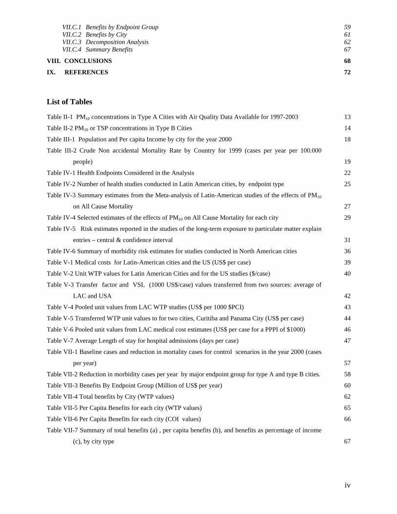
VII.C.1 Benefits by Endpoint Group 59 VII.C.2 Benefits by City 61 VII.C.3 Decomposition Analysis 62 VII.C.4 Summary Benefits 67

VIII. CONCLUSIONS 68 IX. REFERENCES 72

List of Tables

Table II-1 PM10 concentrations in Type A Cities with Air Quality Data Available for 1997-2003 13 Table II-2 PM10 or TSP concentrations in Type B Cities 14 Table III-1 Population and Per capita Income by city for the year 2000 18 Table III-2 Crude Non accidental Mortality Rate by Country for 1999 (cases per year per 100.000

people) 19 Table IV-1 Health Endpoints Considered in the Analysis 22 Table IV-2 Number of health studies conducted in Latin American cities, by endpoint type 25 Table IV-3 Summary estimates from the Meta-analysis of Latin-American studies of the effects of PM10

on All Cause Mortality 27 Table IV-4 Selected estimates of the effects of PM10 on All Cause Mortality for each city 29 Table IV-5 Risk estimates reported in the studies of the long-term exposure to particulate matter explain

entries – central & confidence interval 31 Table IV-6 Summary of morbidity risk estimates for studies conducted in North American cities 36 Table V-1 Medical costs for Latin-American cities and the US (US$ per case) 39 Table V-2 Unit WTP values for Latin American Cities and for the US studies ($/case) 40 Table V-3 Transfer factor and VSL (1000 US$/case) values transferred from two sources: average of

LAC and USA 42 Table V-4 Pooled unit values from LAC WTP studies (US$ per 1000 $PCI) 43 Table V-5 Transferred WTP unit values to for two cities, Curitiba and Panama City (US$ per case) 44 Table V-6 Pooled unit values from LAC medical cost estimates (US$ per case for a PPPI of $1000) 46 Table V-7 Average Length of stay for hospital admissions (days per case) 47 Table VII-1 Baseline cases and reduction in mortality cases for control scenarios in the year 2000 (cases

per year) 57 Table VII-2 Reduction in morbidity cases per year by major endpoint group for type A and type B cities. 58 Table VII-3 Benefits By Endpoint Group (Million of US$ per year) 60 Table VII-4 Total benefits by City (WTP values) 62 Table VII-5 Per Capita Benefits for each city (WTP values) 65 Table VII-6 Per Capita Benefits for each city (COI values) 66 Table VII-7 Summary of total benefits (a) , per capita benefits (b), and benefits as percentage of income

(c), by city type 67

v

List of Figures

Figure I-1 Damage Function Approach 6 Figure IV-1 Comparison of summary results of the effects of PM10 on All Cause 30 Figure IV-2 Concentration-response functions for mortality endpoints. 33 Figure VII-1 Baseline and two control scenarios for PM10 concentrations reductions, by city (µg/m3

annual average). 53 Figure VII-2 Population exposure by age group and PM concentration 54

vi

Executive Summary

Recent estimates indicate that over 100 million people in Latin America and the Caribbean are

exposed to air pollution levels exceeding World Health Organization guidelines. This figure does

not include the millions of individuals who are exposed to indoor air pollution due to biomass

burning and other smaller scale sources, especially in rural areas. Health problems due to poor

air quality have been among the main environmental concerns in Mexico City, Santiago, Bogotá,

Sao Paulo, Lima, Quito among other cities in the region. During the last two decades, several

countries in Latin America have begun to deal more seriously with this environmental problem.

In addition to strengthening environmental institutions and upgrading environmental

measurement systems, environmental standards have been imposed throughout the region,

especially for industries, new and old vehicles, and fuel quality.

Despite this progress, however, the level of knowledge about air pollution’s impact on health is

limited in much of the LAC region, even though it is considered a medium to high priority issue.

Information on air quality remains limited and of uncertain quality in a number of locations.

Moreover, the social costs of health damages from urban air pollution have not yet received

systematic study except in a few locations.

This study provides quantitative estimates of key air pollution concentrations, health impacts,

and the monetary value of improving air quality in 41 major LAC urban areas containing 100

million people in all. While the estimates we derive are necessarily incomplete and uncertain,

they allow comparisons across cities and show the significance of air quality improvements for

the region as a whole. From a policy perspective, the estimates highlight the real economic value

of improvements in urban air quality and give policy analysts a basis for analyzing policies and

abatement measures for their net benefits to society.

“Integrated Assessment” Approach

The approach taken in this study is an example of what is known by policy analysts as

“integrated assessment” using a “damage function” approach. An integrated assessment is a

multidisciplinary, multi-step modeling approach to problems, in this case to the estimation of

economic and physical benefits to health of air pollution improvement. The integrated

assessment approach is shown in Figure E-1.

vii

Figure E-1 Damage Function Approach

This approach involves a series of interlocked components beginning with changes in ambient

air pollution concentrations and ending in societal benefits, using data and models drawn from

government institutions and the academic literature. This report is organized by these

components.

Scope of the Study

For this study we use data on particulate matter (PM-10, specifically). Reasonably plentiful and

usable data are available for this pollutant, and it is strongly identified with problems of illness

and premature mortality based on a large international epidemiology literature. While there are

many air pollutants that can cause health problems, the pollutants of higher concern in LAC are

particulate matter and ground level ozone precursors.* However, usable ozone data are scarce in

Latin America, and in those locations where data are available, the benefits of PM-10 reduction

appear to be on the order of 10 times greater than the benefits of ozone reduction. These figures

* Lead from motor fuel is another serious threat to public health, but the region has already made considerable progress in reducing fuel lead levels and data on blood lead levels were not readily accessible to us. We also recognize that hazardous air pollutants are present in most Latin American cities; however, there is no systematic information on the importance of these pollutants in the different cities.

viii

suggest that the downward bias in our estimates from exclusion of ground level ozone impacts is

not too large.

Scenarios

To represent the variety of different information sources and uncertainties surrounding our

analysis, we constructed several scenarios. We consider two air quality improvement scenarios:

(C1) a uniform reduction of 10% in the annual ambient concentration of PM10 in each city; and

(C2) a scenario in which each city complies with a reference concentration equal to the current

US annual standard for PM10 (50 µg/m3). Under scenario (C1) every city cuts emissions; the

cities with the highest baseline make the largest pollution reduction. Under scenario C2, the

cities with concentrations already below the standard do nothing. Since the cities above the

standard in this case generally have quite poor air quality, the reductions in these cities are well

in excess of those in C1.

To calculate health impacts of the two air quality improvement scenarios, we used two different

pools of statistical information on public health. (E1) Latin American studies; and (E2)

application of U.S. models to our Latin American cities. The results in E1 may be more likely to

reflect actual conditions in Latin America, but the U.S. based analysis E2 is more

comprehensive.

To calculate the economic benefits of improved air quality, we similarly considered two possible

sets of information: (V1) results from a still limited set of economic valuation studies in Latin

America, and (V2) application of valuations from the U.S. to the Latin American cities, after

adjusting for income differences to re-scale the U.S. values. We also considered in each case

two different definitions of economic value. The more conservative measure considers only the

direct savings in the overall social cost of illness (COI): avoided medical costs and lost

productivity from illness. The more comprehensive and theoretically preferable economic

measure includes as well imputed values of indirect, “quality of life” benefits, notably the benefit

enjoyed by everyone in a cleaner environment of a reduced risk of premature death. Assessing

such benefits is more complex and controversial, but they are as or more important in the

assessment of a society’s “willingness to pay” (WTP) for improved air quality as the direct

savings from illness costs.

ix

Key Findings

Figure E-2 shows the kinds of reductions in particulate matter implied by our two air quality

scenarios. Our survey of available air quality data indicates that 26 cities, containing 85 million

people (of which 28 million are children less than 18 years of age) out of the almost 100 million

population of the cities considered in the study, are exposed to particulate concentrations above

internationally accepted levels. For many of them (18 million, 6 of them children), the excess is

notably large (more than twice the US standard). We must also note, however, that for many of

the cities we have considered, particulate data are of very uncertain quality. For almost all cities,

moreover, data on ground level ozone or its precursors is very elusive. Based on the general

principle that good policy flows from good data as well as sound analysis, improvement in air

quality monitoring in Latin America should be a higher priority than it evidently is at the present

time.

The physical effects on health of these excess pollution levels also are quite significant. If we

look only at cities with PM concentrations above the U.S. standard, reducing concentrations to

the level of the standard would avoid on the order of 10,500 to 13,500. premature deaths as well

as well a host of illness incidents, reduced activity days, and lost productivity. The premature

deaths avoided from this air quality improvement would occur across the age distribution but

would be especially important for more sensitive elder and child populations (by some of our

estimates, 10,000 and 2,500 excess deaths avoided in these groups, respectively). The total

premature deaths avoided would be on the order of 2 to 2.6% of total deaths per annum in the

cities considered.

Health improvements occur not just from reducing PM concentrations to meet the U.S. standard

but also through further improvements below the standard. Our simulation of a 10% reduction in

concentrations in all cities also led to large reductions in illness and premature mortality, with

benefits spread out over the range of cities. Indeed, for this scenario the deaths avoided in cities

meeting the standard are 12 to 25% of total deaths avoided, suggesting that just meeting the U.S.

standard should not automatically be seen as an adequate goal. These relatively significant

health benefits are predicted whether one relies on epidemiological studies from Latin America

or on extrapolated application of U.S.-based studies (the latter predicts even larger health

improvements, on the order of 30% more).

x

Figure E-2. Baseline and two control scenarios for PM10

Concentration reductions, by city (µg/m3 annual average)

0 20 40 60 80 100 120 140 160

Cities with Monthly Data -----Campinas, BR

Canoas, BRCubatao, BR

Porto Alegre, BRSao Paulo, BR

Sao Jose Do Campos, BRSorocaba, BR

Vitoria, BRCalama, CL

Santiago, CLTemuco, CLBogota, CO

Cali, COGuadalajara, MX

Juarez, MXMexico City, MX

Monterrey, MXValle De Toluca, MX

Panama City, PAKingston, JA

Cities with Annual Data ------Buenos Aires, AR

Cordoba, ARMendoza, AR

Caxias, BRCuritiba, BRItaguai, BR

Rio De Janeiro, BRSao Joao De Meriti, BR

Heredia, CRSan Jose, CRGuayaquil, EC

Quito, ECSan Salvador, ESTegucigalpa, HO

Managua, NILima, PE

Montevideo, URCaracas, VZ

ug/m3

Reduction in C2 (less C1)

Reduction in C1

Table E-1 below summarizes the findings of the economic analysis. The valuations based on a

combination of U.S based health impacts models, and transfer of U.S valuations to Latin

America, exceed those based only on Latin American health models and valuations by a factor of

approximately 12 for the more inclusive Willingess to pay estimates, and 17 for cost of illness

estimates. This further highlights the need to develop better estimates of Latin American

valuations comparable to the more comprehensive U.S based measures. The findings also are

sensitive to the difference between direct cost savings and the more comprehensive willingness

to pay measure for valuing health improvements. Economic analysis makes a solid case for use

of the broader and more inclusive measure. But the more intangible benefits do not register in

the national accounts, for example, and with scarce resources there may be some pressure in the

policy process to scale investments in air pollution control to the more modest level implied by

cost of illness assessments of benefits.

xi

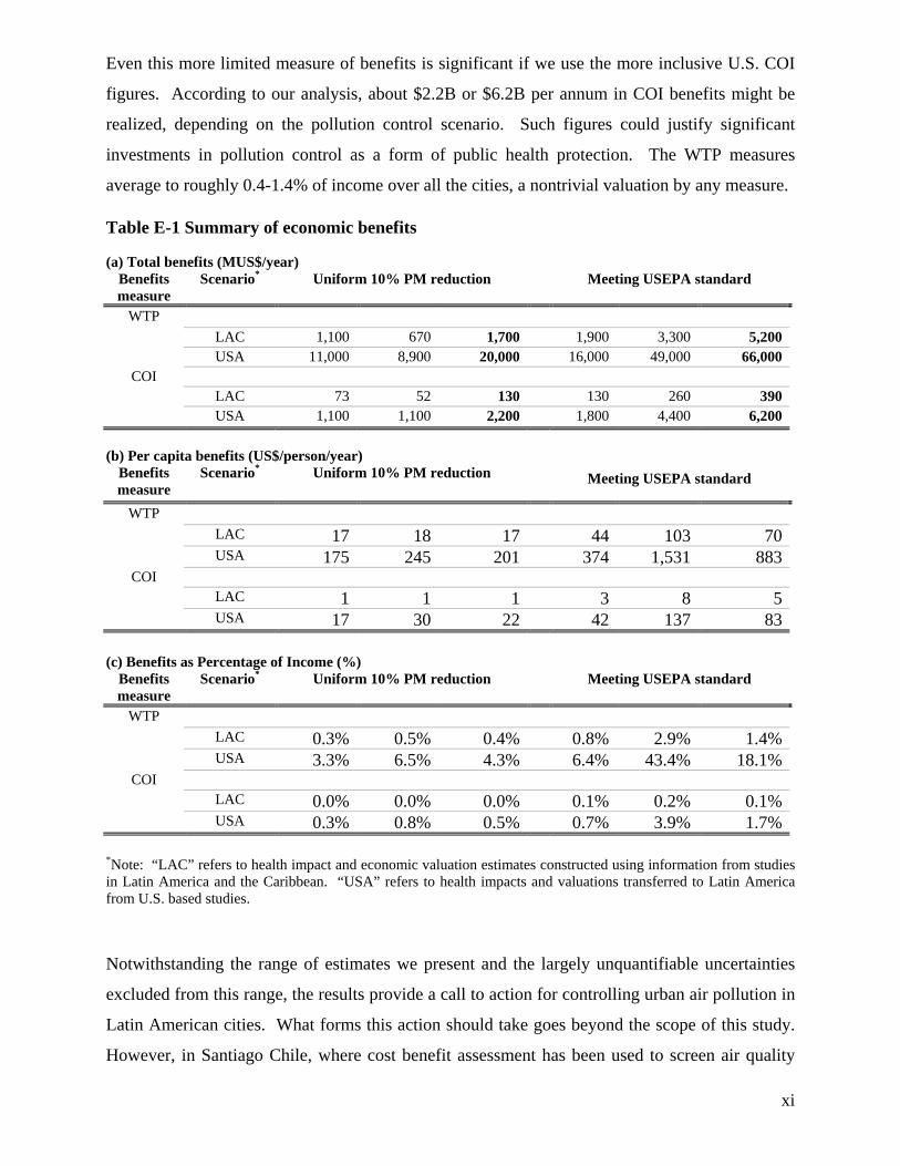
Even this more limited measure of benefits is significant if we use the more inclusive U.S. COI

figures. According to our analysis, about $2.2B or $6.2B per annum in COI benefits might be

realized, depending on the pollution control scenario. Such figures could justify significant

investments in pollution control as a form of public health protection. The WTP measures

average to roughly 0.4-1.4% of income over all the cities, a nontrivial valuation by any measure.

Table E-1 Summary of economic benefits

(a) Total benefits (MUS$/year) Benefits measure

Scenario* Uniform 10% PM reduction Meeting USEPA standard

WTP LAC 1,100 670 1,700 1,900 3,300 5,200 USA 11,000 8,900 20,000 16,000 49,000 66,000

COI LAC 73 52 130 130 260 390 USA 1,100 1,100 2,200 1,800 4,400 6,200

(b) Per capita benefits (US$/person/year)

Benefits measure

Scenario* Uniform 10% PM reduction Meeting USEPA standard

WTP LAC 17 18 17 44 103 70 USA 175 245 201 374 1,531 883

COI LAC 1 1 1 3 8 5 USA 17 30 22 42 137 83

(c) Benefits as Percentage of Income (%)

Benefits measure

Scenario* Uniform 10% PM reduction Meeting USEPA standard

WTP LAC 0.3% 0.5% 0.4% 0.8% 2.9% 1.4% USA 3.3% 6.5% 4.3% 6.4% 43.4% 18.1%

COI LAC 0.0% 0.0% 0.0% 0.1% 0.2% 0.1% USA 0.3% 0.8% 0.5% 0.7% 3.9% 1.7%

*Note: “LAC” refers to health impact and economic valuation estimates constructed using information from studies in Latin America and the Caribbean. “USA” refers to health impacts and valuations transferred to Latin America from U.S. based studies. Notwithstanding the range of estimates we present and the largely unquantifiable uncertainties

excluded from this range, the results provide a call to action for controlling urban air pollution in

Latin American cities. What forms this action should take goes beyond the scope of this study.

However, in Santiago Chile, where cost benefit assessment has been used to screen air quality

xii

improvement options, benefits information of the type we have generated has been used with

cost information to lay out a menu of potential interventions. These include new emission

standards for fixed and mobile sources (new buses, trucks, and automobiles), the retrofit of

existing diesel vehicles with particle traps, the introduction of very-low sulfur diesel fuel, and the

introduction of an emissions cap and trade system to improve efficacy and cost-effectiveness of

emissions limitations for fixed sources.

The cost-effectiveness of different interventions is sector and country-specific. Generally,

simple PM filtration measures at stationary sources can be cost effective, as can be some targeted

measures to reduce emissions from older diesel vehicles or to introduce low sulfur diesel fuel.

How far these and other interventions can be taken while still yielding net benefits – and widely

shared benefits – requires more detailed analysis of mitigation costs. What our analysis may

offer from a policy perspective, among other points, is a stronger rationale for investigating

policy options and then robustly implementing those policies that can be justified.

1

I. Introduction

Recent estimates cited in a survey conducted by the Pan American Center for Sanitary

Engineering and Environmental Sciences (PAHO 2000) indicate that over 100 million people in

Latin America and the Caribbean are exposed to air pollution levels exceeding World Health

Organization guidelines. This figure does not include the millions of individuals who are

exposed to indoor air pollution due to biomass burning and other smaller scale sources,

especially in rural areas. During the last two decades, several countries in Latin America have

begun to deal more seriously with this environmental problem.1 In addition to strengthening

environmental institutions and upgrading environmental measurement systems, environmental

standards have been imposed throughout the region, especially for industries, new and old

vehicles, and fuel quality.

Despite this progress, however, the level of knowledge about air pollution’s impact on health is

limited in much of the LAC region, even though it is considered a medium to high priority issue.

Information on air quality remains limited and of uncertain quality in a number of locations.

Moreover, the social costs of health damages from urban air pollution have not yet received

systematic study except in a few locations.2 Our aim in this study is to shrink this information

gap by providing quantitative estimates of air pollution concentrations, as well as health effects

and the monetary value of improving air quality in 41 major LAC urban areas containing 100

million people in all.

While the estimates we derive are necessarily incomplete and uncertain, they allow comparisons

across cities and show the significance of air quality improvements for the region as a whole.

This study is the first to collect and analyze together virtually all of the accessible air quality,

health and economic valuation data from Latin America. We also utilize health and economic

valuation data from the U.S., adjusted to apply to Latin America, in order to provide additional

perspective on the benefits of air quality improvements. From a policy perspective, the estimates

highlight the real economic value of improvements in urban air quality and give policy analysts a

basis for analyzing policies and abatement measures for their net benefits to society.

1 Health problems due to poor air quality have been among the main environmental concerns in Mexico City, Santiago, Bogotá, Sao Paulo, Lima, Quito among other cities in the region.

2

As reported in Section VII of the paper, we find that economic benefits of air quality

improvement are significant in terms of both reduction of disease incidence and economic well-

being. To put these findings into a broader perspective, the Global Burden of Disease (GBD)

project has identified environmental risks as a significant component of the overall burden of

disease (Ezzati, Lopez et al. 2002). Depending on gender and on the health impact measure used,

environmental risks generally are roughly 4-5% of the total burden of disease risk for a group of

relatively higher income countries in Latin America and the Caribbean, and 7-9% for a group of

relatively lower income countries (including Bolivia, Ecuador, Guatemala, Haiti, Nicaragua, and

Peru). This makes environmental risks roughly comparable to childhood and maternal under-

nutrition and ahead of sexual and reproductive health risks, though behind (for men) addictive

behaviors like smoking.

The largest single environmental component is unsafe water, sanitation, and hygiene – especially

in the poorer country group. Urban air pollution in and of itself is a smaller component of the

overall environmental risk. However, when the GBD looks globally (not just in Latin America)

at leading causes of disease, lower respiratory disease ranks second, right behind HIV. Since

dirty urban air can aggravate sensitivity to other airborne health threats (including smoking and

dirty cooking fuels), interventions to improve air quality have overall impacts beyond their direct

effects by reducing the severity of other health insults.

I.A The Fundamentals of Economic Analysis for Air Quality Improvements

I.A.1 Cost-of-Illness Measure of Air Quality Improvement Benefits

Cost-of-illness estimates typically include direct medical expenditures and forgone wages

associated with illness and premature death. Often, the value of lost household services is

included as well. This approach -- also known as the human capital approach when it addresses

premature deaths -- does not purport to be a measure of individual or social welfare, since it

makes no attempt to include intangible but real losses in well-being, such as those associated

with pain and suffering. Its advantage is that it is relatively simple to calculate and understand.

Historically, this has been an important approach used to calculate monetary costs associated

2 These include Santiago, Mexico City, and Sao Paolo, as discussed below.

3

with illness and death. The U.S. Department of Agriculture (USDA) and the Centers for Disease

Control and Prevention (CDC), in particular, feature this measure in their cost-benefit analyses

(Buzby, Roberts et al. 1996). The USDA has recently issued a Cost of Illness Calculator

((Economic Research Service - USDA 2003) for application to food borne illnesses. Cost-of-

illness measures are generally at least several times lower than WTP measures for the same

health effect, because of their exclusion of intangible values (Kulcher and Golan 1999).

I.A.2 Willingness to Pay (WTP) Measure of Air Quality Improvement Benefits3

The WTP approach is a benefits-based measure versus the limited cost-based COI approach. It

is rooted in on the tradeoffs that individuals make between health and wealth or income (or other

goods). Such tradeoffs in daily life are easily recognized and sometimes observed. For example,

if a person is running late to a meeting he may drive faster, knowing that the increased speed

carries with it a slightly increased chance of accident and possibly death. Or a person may take a

riskier job if he knows the pay will be higher to compensate for the greater accident risk (or the

converse: he may be content with a less risky job making lower wages).

WTP values can be divided into those measuring preferences for reductions in the risk of

premature death, and those measuring preferences for reductions in morbidity (illness) risk.

Morbidity can be divided into acute effects and incidence of chronic disease. For valuation

purposes, the acute effects are usually modeled and estimated as though they are certain to be

avoided, whereas the chronic effects are usually treated in the same way as for mortality i.e., as a

reduction in the risk of developing a chronic disease.4 Values to reduce acute effects, the

probability of chronic effects and the probability of premature death are usually added up, with

some minor adjustments to avoid obvious double-counting.5

3 Another measure of preferences consistent with welfare economics is willingness to accept (WTA). This approach has been difficult to implement in practice because of ethical issues (e.g., how much money would you accept to not have your risks reduced) and technical reasons, i.e., your answer in unbounded by income so dispersion of answers tends to be very wide. Consequently, WTP is the preferred measure.

4 Estimates of the WTP for mortality risk reductions are sometimes converted to a “value of statistical life” (VSL) by dividing the WTP by the risk change being valued. Similarly, the value of a statistical case of chronic illness is (the WTP for a risk reduction in chronic illness)/(risk change).

5 Recently, DeShazo and Cameron (2003) have administered surveys that ask for preference rankings over lifecycle-based health effects and mortality risks, offering the possibility of monetizing preferences for mortality and morbidity holistically.

4

WTP studies attempt to estimate economic benefits based on individual preferences either by

uncovering the tradeoffs people actually make (revealed preference (RP)) or by presenting

people with hypothetical but realistic choices in a survey-based approach (stated preference

(SP)). The revealed preference approach involves examining behavior, either in the marketplace

or elsewhere, to discern WTP. There are a wide variety of revealed-preference approaches. The

most developed technique for estimation of health and mortality risk reduction benefits is

probably the hedonic-labor-market approach and the property-value approach. The most

common RP approach, and the approach whose studies have traditionally under girded VSL

estimates used by the government in CBAs, is the hedonic-labor-market approach. This

approach involves estimating the wage premiums paid to workers in jobs that have high risks of

death (Viscusi 1992; Viscusi 1993; Viscusi and Aldy 2002).

Under the stated preference approach, two approaches are in use. Contingent valuation (CV)

studies pose questions about the willingness to pay (WTP) for a change in risk of an adverse

health outcome. A newer alternative to CV is conjoint analysis, which is used extensively in

marketing to elicit preferences for combinations of product attributes. When such analyses

involve the attribute of a price, the value placed on other attributes can be estimated.

SP and RP methods have been most extensively used to estimate WTP for reductions in risks of

death. The SP methods involve placing people in realistic, if hypothetical, choice settings and

eliciting their preferences. In CV surveys, individuals are not asked how much they value life

per se, because WTP to avoid certain death is limited only by wealth. However, as has been

observed in many cases, people are willing to make tradeoffs between marginal changes in risk

and wealth. These choices might involve alternative government programs or specific states of

nature, such as a given reduction in one's risk of death in an auto accident associated with living

in one city instead of another, riskier, city (see (Krupnick and Cropper 1992)) or choosing

between two bus companies with different safety records when deciding to ride a bus (Jones-Lee,

Hammerton et al. 1985) . Therefore, attempts are made to ascertain WTP to reduce the chance of

death by some small probability. Framing the question in this way highlights an important point:

a WTP estimate for mortality risk reduction does not provide an inherent value for human life;

rather it illuminates the choices and tradeoffs that individuals are willing to make and converts

those choices into a value for a statistical life (VSL) by aggregating over many people their WTP

for small changes in risk.

5

Calculating the implied value of health outcomes from WTP studies is usually straightforward.

Using the “damage function” approach or “integrated assessment,” (see below), the unit values

for the different endpoints are multiplied by the expected change in the incidence of the effect,

taken from physical response functions in the literature. However, it is also possible to

determine total WTP without going through the step of applying values to expected outcomes.6

An important issue bearing on the validity of monetary valuation is its applicability to the

context in which it is used. Most studies are site-specific and coverage of all possible sites and

situations is impossible. Therefore, it is often necessary to transfer the results of a study that

focuses on one specific situation to another study with a different location or setting of interest.

This procedure is known as benefit transfer, and there are occasions when the reliability of

valuation estimates can be questioned. For example, hedonic wage studies provide mortality risk

reduction valuations based on accidental deaths of prime working-age individuals. It can be

argued that this context is inappropriate for estimating the benefits of pollution control, where

older and ill individuals are most at risk

In the area of estimating WTP for health outcomes, there is a vast literature including

pronouncements from expert committees on appropriate protocols. The so-called National

Oceanic and Atmospheric Administration (NOAA) Panel (Arrow, Solow et al. 1993), made up of

several Nobel laureate economists, survey researchers and others, developed recommendations

about how to conduct credible stated preference studies on the valuation of natural resources,

recommendations that generally carry over to health valuation.7 Major books and articles on

WTP methods include (Mitchell and Carson 1989; Freeman III 2003) (Carson, Flores et al. 2001)

(Carson, Hanemann et al. 1996) (Cummings, Brookshire et al. 1986) (Alberini, Krupnick et al.

2003), and (Champ, Boyle et al. 2003). In addition, a variety of computer models and modeling

efforts have codified the health valuation literature. See, in particular, (EPA 1999), (Rowe and al

1995), (Farrow, Wong et al. 2001), and (European Commission 1999). We know of only one

6 For instance, in measuring the WTP to reduce air pollution using housing price variation over space, the physical effects measure is embedded in perceptions of homebuyers and sellers about what would happen to their health if they live in homes at locations with different degrees of air pollution. Because this approach uses public perceptions of dose-response relationships rather than scientifically-based relationships, it has fallen into disuse in favor of the damage function approach.

7 The NOAA panel was convened to sort out competing claims about the credibility of CV surveys on existence value in the wake of the Exxon Valdez oil spill in Prince William Sound, Alaska.

6

study that has tried to estimate the WTP for mortality risk reductions in Latin America,

conducted by one of the authors, in Santiago, Chile, during 1999 (Cifuentes, Prieto et al. 2000) .

I.B “Integrated Assessment” Approach

The approach taken in this study to implement the economic analysis sketched above is an

example of what is known by policy analysts as “integrated assessment” using the “damage

function” approach. An integrated assessment is a multidisciplinary, multi-step modeling

approach to problems, in this case to the estimation of economic and physical benefits to health

of air pollution improvement. The integrated assessment approach is shown in Figure I-1.

Figure I-1 Damage Function Approach

This approach involves a series of interlocked components beginning with changes in ambient

air pollution concentrations and ending in societal benefits, using data and models drawn from

government institutions and the academic literature. This report is organized by these

components.

7

I.C Scope of the Study

The air quality data we use for the study are centered on particulate matter (PM-10, specifically).

We note here that the study emphasizes PM-10 not just because usable data are available for this

pollutant, but also because of its strong identification in problems of illness and premature

mortality based on a large international epidemiology literature (Holgate, Samet et al. 1999).

There are many air pollutants that can cause health problems. The most common ones are

referred to as “criteria pollutants” and include particulate matter (PM10 or PM2.5), SO2, NO2, CO,

O3 and lead. Although all of them are known to cause health problems, the pollutants of higher

concern in LAC are particulate matter and ozone, which is itself an indicator of many other

oxidants present in the air.

Usually, health impact analyses consider these two pollutants, which represent two more or less

independent sources of impacts. However, in this project we undertake the estimation of PM10 -

related impacts only. This is based on the availability of data (which are seldom sufficiently

available for analysis of O3 reduction benefits). ) There is a difficulty in that ozone is more

heterogeneous both temporally and geographically than PM10, making computations with ozone

more difficult. Further, what most cities report is the number of exceedances of the ozone

standard, or the maximum one hour level during a month. From that information it is not possible

to compute the health effect

Two cities in which the impacts of PM and O3 have been estimated recently are Mexico City and

Santiago, Chile. According to Molina and Molina (2002), the benefits from a reduction of 10%

in PM10 and ozone levels in the Metropolitan Area of the Valley of Mexico in the year 2000 are

about $2 billion for PM10 and only $200 million for ozone. 8 In Santiago, the benefits of the

Decontamination Plan were assessed by one of the authors (Cifuentes, 2001) in a report for the

Chilean Environmental Commission. The total benefits from PM2.5 reductions likewise were

about 10 times the benefits from ozone reductions. These figures suggest that the downward bias

in our estimates from exclusion of ozone is not too large.

8 However they did not considered hospital admissions, which are high for ozone, in their calculations. The study by Cesar et al (2000) shows a different picture. For a 10% reduction in pollution levels, ozone benefits are 70% of those of PM10 when WTP is considered. When only cost of illness and human capital losses are considered, ozone benefits are 3 times those of PM10. This is because most of ozone effects are hospital admissions, which account for a big fraction of COI benefits. For an scenario in which the air quality standards are attained for both pollutants, ozone benefits are 2 and 8.8 times those of PM10 for COI and WTP values respectively .This higher

8

Lead from motor fuel is another serious threat to public health, but the region has already made

considerable progress in reducing fuel lead levels and data on blood lead levels were not readily

accessible to us9. We also recognize that hazardous air pollutants are present in most Latin

American cities; however, there is no systematic information on the importance of these

pollutants in the different cities.

This section is followed by a description of population and other baseline incidence data needed

for estimating health improvements and benefits. The following section focuses on the

epidemiological literature linking changes in air quality to human health. This section is

followed by another on the economic health valuation literature. The remainder of the paper

presents the main results and conclusions.

II. Air Quality Data in Latin American Cities

This section presents the air quality data in Latin American cities that will be used in this report

to estimate the health benefits that can be obtained from reducing air pollution. There is also a

brief discussion of the main sources of pollution in these cities. A significant effort has been

made to identify cities with “solid” air quality data as well as other cities where the available

information gives some idea as to the magnitude of the problem but is less reliable.

II.A Main Sources of Air Pollution in LAC

The urbanization process in Latin America is an ongoing process. Currently about 75% of the

population of Latin America and the Caribbean live in cities (UNEP 2002). Several megacities

such as Buenos Aires, Mexico City, Rio de Janeiro and Sao Paulo, each with a population of

more than 10 million, are located in the region and economic growth in these urban centers has

caused increases in air pollution (particularly CO, NOx, SO2, tropospheric ozone (O3),

hydrocarbons and particulates) and associated human health impacts (UNEP, 2000).

value is due to the fact that the percentage reductions required to attain the O3 standard are much higher than those for PM10.

9 Concentrations of lead have been reduced since most of the countries in Latin America have eliminated lead from their fuel or are in the process of doing so. In South America there are only five countries still supplying leaded fuels: Uruguay, Venezuela, Cuba, Peru and French Guinea. Also, some of their Caribbean Islands still use leaded fuel. It is believed that lead will be completely phased out in the region throughout the next decade. See for example http://www.walshcarlines.com/pdf/leadphaseoutupdate.pdf.

9

There are many sources that are responsible for emissions of particulates and particulate

precursors, including SO2 and NOx. Transport activity is a main source of direct and indirect

pollution, especially in larger cities, but also increasingly in medium sized cities. It is estimated

that over 40% of emissions of PM10 in Mexico City and 86% in Santiago come from the

transport activity10. In addition, NOx emissions from transport in both cities account for more

than 75% of total emissions of NOX (O'Ryan and Larraguibel 2000). On the other hand

emissions from fixed sources only account for 7% and 14% in Santiago (for PM10 and NOX) and

around 15% and 12% in Mexico City. However, the lack of knowledge, even in these two more

advanced countries in terms of air pollution control is significant. For example in Santiago the

characterization of particulates obtained from filters shows a different mix for the sources

responsible for PM10: 49% mobile sources, 29% for fixed sources including industry and

residential and 22% for area sources (CONAMA RM, 2001).

Direct emissions from vehicles as well as suspended particles from dust, both on paved and

unpaved roads, are responsible for an important amount of air pollution. Fuel quality -

particularly sulfur content in gasoline and diesel fuel- is a key factor that determines the amount

of SO2 emissions, which contribute to PM10 when converted in the air to sulfates. As a

comparison sulfur contents in diesel fuel in Brazilian cities reach up to 1000 ppm, while in

Mexico City these are currently 500 ppm and Santiago, Chile these have been reduced from 500

to 300 ppm in 2001 and to 50 ppm in mid 2004. For comparison, the US and Canada now limit

the sulfur content to 500 ppm, while most European countries require 50 ppm, but some

(Denmark, Sweden) limit it to 15 ppm) (Walsh 2005).

Old car, truck and bus fleets in Latin America are an important factor. Whereas on average

vehicle turnover in the US is relatively rapid, it is not uncommon for cars in cities of Latin

America to be 10 or even 20 and more years old. Another related factor is the inadequate

maintenance of engines. In many cities, the main source of pollution is old diesel-fuel buses and

trucks with poor maintenance, which contribute heavily towards total emissions11. Excess

circulation of buses in off-peak hours due to the need to finance the fixed costs of small bus-

owners adds significantly to emissions in some cities. Finally the last source of air pollution from

10 This latter number includes direct emissions from combustion and indirect emissions from paved and unpaved

roads. 11 For example diesel buses and trucks in Santiago contribute up 46% of total direct emissions of particulates (not

including resuspended particles) and 54% of emissions of NOx (CONAMA. 2002).

10

transport is related to driving patterns and congestion. Poor driving patterns (e.g., excess

acceleration and deceleration) can increase total emissions of different pollutants significantly. A

recent study for Santiago showed that improving driving conditions in public buses can reduce

emissions of CO, VOCs, NOx and particulates in over 25%. Additional studies in Argentina and

Mexico show similar results.

The second main source of pollution in Latin America comes from industrial activities. In

several cities, industrial activity is still an important source of air pollution emissions. However

several larger cities have attacked the problem by imposing and enforcing emission standards for

industrial sources. Such is the case for example, for Santiago and Mexico City as well as in

Quito and Bogotá. However there are still some cities with heavy industrial air pollution such as

Cubatao in Brazil.

In certain specific areas the air pollution problem is not related to vehicles or industrial activity,

but rather to residential use of fuel wood for cooking and/or heating as in Temuco and other mid

sized cities in the south of Chile and some Central American countries; forest fires such as in

Central America, or even a volcano eruptions as in Quito, Ecuador in 1999 (UNEP 2002).

Unfavorable topographic and meteorological conditions in some cities aggravate the impact of

air pollution: the Valley of Mexico obstructs the dispersal of pollutants from its metropolitan

area as do the hills surrounding Santiago (ECLAC 2000). This is perhaps more of a problem for

ozone than PM10.

In summary, most PM10 pollution problems in Latin American cities can be related to the

transport sector. However, a few cities do not follow this pattern and the main sources of high

PM-10 concentrations are either industrial activity or residential use of fuel-wood. Since growth

in income for developing countries in LAC is expected, it is very likely that vehicle-related

emissions will increase significantly as more people have access to cars.

II.B The challenge of finding air quality data

Compiling air quality data in Latin America requires a significant effort. A first problem is that

the existing data are not readily available and the quality of the data is usually not known except

by a few local experts. Consequently, where the information exists, often a visit or a contact with

a local official is required to obtain it and assess its quality. On other occasions the information

does not exist at all or is outdated.

11

Continuity of the information is another problem and the task of building a time series of

acceptable quality is very difficult, with few exceptions. Regular air monitoring networks are

expensive to set up, operate and maintain. For example, the monitoring network in Santiago cost

US$ 2 million to implement and requires each year approximately US$ 0.5 million to operate

and maintain. As a result in many cities there are air quality studies for only one or two short

periods. This makes it difficult to establish whether the information obtained is of good quality

and representative enough of the state of the environment. In many cases different methodologies

are used to measure air quality in different studies that may not be comparable.

Access to the available information is another problem. Recently the use of information

technologies, especially the Internet, has allowed part of the data collection process to be

speeded up. Nevertheless, the process is still slow and complicated. Information technologies

have not been taken advantage of to produce comparable data sets for different Latin American

cities that could make the search for information less cumbersome and uncertain. Another issue

is that on many occasions the information is not publicly released –so it may exist but not be

accessible- or it may not be released to the extent needed for credible research.

II.C Air Quality in Latin American Cities

Based on expert judgment the air quality situation is presented for 21 cities with reliable

information (type A cities), and for 18 cities with data that are more uncertain but that are

expected to reflect typical annual averages, for a total of 39 cities.

The data are the result of a combination of readily available data from internet, communications

with local experts in Latin American cities and expert opinion on the quality of the data from the

research team. An effort has been made to include all major cities for which experts concur there

are or could be air pollution problems and to ensure that the information for the key cities

considered is of reasonable quality. The numbers presented may not include a city for which

there is acceptable information, simply because the information was not readily accessible,

however these cities should be few. Similarly, the quality of the information in all cities is not

the same, so cities with more reliable information have been grouped by data quality based on

expert judgment12.

12 In general type B cities lack a monthly data.

12

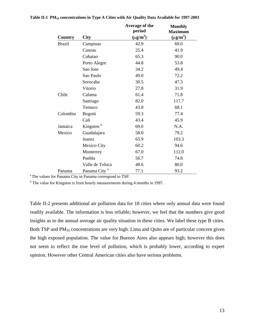
Several countries including Brazil, Mexico, Colombia and Chile have regular monitoring

programs that have followed USEPA guidelines. There is local expertise and the data from these

cities can be considered of good quality. This information together with that of Panama City and

Kingston, Jamaica for 1997-2003, is included in Table II-2 and comprises 21 cities with data that

can be considered of good quality13. The first two columns identify the country and city for

which data were found. The next two columns show the average and monthly maximum of PM10

concentrations in each city except for Santa Marta and Panama City where TSP was considered.

Clearly, air quality is an issue in both large and small cities. Almost all cities, except four small

Brazilian cities (Canoas, Sao Jose, Sorocaba and Vitorio), have annual averages over 40 µg/m3,

and higher monthly maximum levels. This suggests that probably all cities would benefit

significantly from reducing air pollution. Santiago has the worst PM10 pollution problem, but

Ciudad Juarez, Monterrey and Mexico City also have serious episodes at some time of the year.

Cubatao, Bogotá, Guadalajara, Toluca also appear to have problems since their maximum

monthly average is over 75 µg/m3.

13 Panama City has monthly data for a specific period but not a regular monitoring program. Similarly, Kingston had a program in 1997 in which a continuous monitoring network was undertaken based on hourly measurements in several sites during a four month period.

13

Table II-1 PM10 concentrations in Type A Cities with Air Quality Data Available for 1997-2003

Country City

Average of the period (µg/m3)

Monthly Maximum

(µg/m3) Brazil Campinas 42.9 69.0 Canoas 25.4 41.9 Cubatao 65.3 90.0 Porto Alegre 44.8 53.8 Sao Jose 34.2 49.4 Sao Paulo 49.0 72.2 Sorocaba 30.5 47.3 Vitorio 27.8 31.9 Chile Calama 61.4 71.8 Santiago 82.0 117.7 Temuco 43.8 68.1 Colombia Bogotá 59.3 77.4 Cali 43.4 45.9 Jamaica Kingston b 69.0 N.A. Mexico Guadalajara 58.0 79.2 Juarez 65.9 103.3 Mexico City 60.2 94.6 Monterrey 67.0 112.0 Puebla 56.7 74.8 Valle de Toluca 48.6 80.0 Panama Panama City a 77.1 93.2

a The values for Panama City in Panama correspond to TSP. b The value for Kingston is from hourly measurements during 4 months in 1997.

Table II-2 presents additional air pollution data for 18 cities where only annual data were found

readily available. The information is less reliable; however, we feel that the numbers give good

insights as to the annual average air quality situation in these cities. We label these type B cities.

Both TSP and PM10 concentrations are very high. Lima and Quito are of particular concern given

the high exposed population. The value for Buenos Aires also appears high; however this does

not seem to reflect the true level of pollution, which is probably lower, according to expert

opinion. However other Central American cities also have serious problems.

14

Table II-2 PM10 or TSP concentrations in Type B Cities

a The period for measurements of PM10 and TSP is not necessarily the same. For example PM10 in Lima was measured for 1999 whereas TSP was measured between 2000 and 2002. For Heredia TSP was measured between 1996 and 1999, while San Jose was measured for 1993-1999: Quito’s data for TSP is for 1994-1998. Finally in Tegucigalpa TSP is for 1994-1999 and PM10 for 1995-1999.

Country City Period a

PM10 Annual Average (µg/m3)

TSP Annual Average (µg/m3)

Argentina Buenos Aires 1997-1998 188.5 Cordoba 1987-1992 154 Mendoza 1997-1998 31.2 Brazil Curitiba 2000-2001 51 D. Caxias 1986-1993 115.6 Itaguai 1989-1996 35.6 Rio De Janeiro 1986-1996 128.1 S.J. Meriti 1986-1996 182.4 Costa Rica Herediaa 1996 76.5 228.3 San Josea 1996-1999 53 200 Ecuador Guayaquila 1994-1995 120.7 Quito 1994-1998 59.5 200.1 El Salvador San Salvadora 1996-1999 62.7 189.4 Honduras Tegucigalpaa 1994-1999 79.4 452.7 Nicaragua Managuaa 1996-1999 60.9 313.8 Peru Limaa 1999 146.4 165.8 Uruguay Montevideo 1998-1999 253.3 Venezuela Caracas 1986-1995 67.8

15

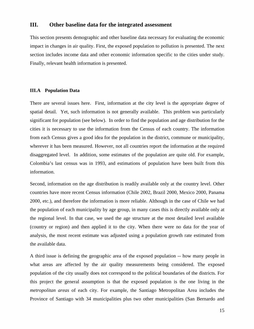
III. Other baseline data for the integrated assessment

This section presents demographic and other baseline data necessary for evaluating the economic

impact in changes in air quality. First, the exposed population to pollution is presented. The next

section includes income data and other economic information specific to the cities under study.

Finally, relevant health information is presented.

III.A Population Data

There are several issues here. First, information at the city level is the appropriate degree of

spatial detail. Yet, such information is not generally available. This problem was particularly

significant for population (see below). In order to find the population and age distribution for the

cities it is necessary to use the information from the Census of each country. The information

from each Census gives a good idea for the population in the district, commune or municipality,

wherever it has been measured. However, not all countries report the information at the required

disaggregated level. In addition, some estimates of the population are quite old. For example,

Colombia’s last census was in 1993, and estimations of population have been built from this

information.

Second, information on the age distribution is readily available only at the country level. Other

countries have more recent Census information (Chile 2002, Brazil 2000, Mexico 2000, Panama

2000, etc.), and therefore the information is more reliable. Although in the case of Chile we had

the population of each municipality by age group, in many cases this is directly available only at

the regional level. In that case, we used the age structure at the most detailed level available

(country or region) and then applied it to the city. When there were no data for the year of

analysis, the most recent estimate was adjusted using a population growth rate estimated from

the available data.

A third issue is defining the geographic area of the exposed population -- how many people in

what areas are affected by the air quality measurements being considered. The exposed

population of the city usually does not correspond to the political boundaries of the districts. For

this project the general assumption is that the exposed population is the one living in the

metropolitan areas of each city. For example, the Santiago Metropolitan Area includes the

Province of Santiago with 34 municipalities plus two other municipalities (San Bernardo and

16

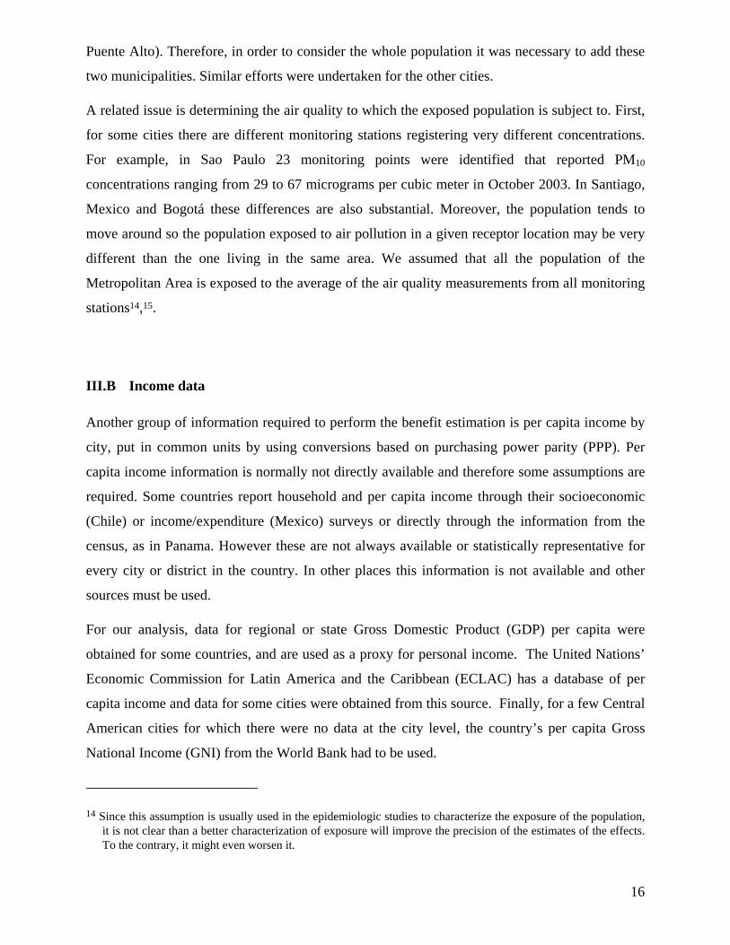
Puente Alto). Therefore, in order to consider the whole population it was necessary to add these

two municipalities. Similar efforts were undertaken for the other cities.

A related issue is determining the air quality to which the exposed population is subject to. First,

for some cities there are different monitoring stations registering very different concentrations.

For example, in Sao Paulo 23 monitoring points were identified that reported PM10

concentrations ranging from 29 to 67 micrograms per cubic meter in October 2003. In Santiago,

Mexico and Bogotá these differences are also substantial. Moreover, the population tends to

move around so the population exposed to air pollution in a given receptor location may be very

different than the one living in the same area. We assumed that all the population of the

Metropolitan Area is exposed to the average of the air quality measurements from all monitoring

stations14,15.

III.B Income data

Another group of information required to perform the benefit estimation is per capita income by

city, put in common units by using conversions based on purchasing power parity (PPP). Per

capita income information is normally not directly available and therefore some assumptions are

required. Some countries report household and per capita income through their socioeconomic

(Chile) or income/expenditure (Mexico) surveys or directly through the information from the

census, as in Panama. However these are not always available or statistically representative for

every city or district in the country. In other places this information is not available and other

sources must be used.

For our analysis, data for regional or state Gross Domestic Product (GDP) per capita were

obtained for some countries, and are used as a proxy for personal income. The United Nations’

Economic Commission for Latin America and the Caribbean (ECLAC) has a database of per

capita income and data for some cities were obtained from this source. Finally, for a few Central

American cities for which there were no data at the city level, the country’s per capita Gross

National Income (GNI) from the World Bank had to be used.

14 Since this assumption is usually used in the epidemiologic studies to characterize the exposure of the population, it is not clear than a better characterization of exposure will improve the precision of the estimates of the effects. To the contrary, it might even worsen it.

17

Purchasing Power Parity income (PPPI) is available from the World Bank only at the country

level. Since income varies for cities of the same country, the PPPI was calculated for each city

by adjusting it in proportion to the ratio of per capita income in the city to the country, as

follows:

country

citycountrycity PCI

PCIPPPIPPPI =

Table III-1 shows the population and income data for the cities and for the countries.

15 An exception is Rio de Janeiro where there are monitoring stations in specific localities that represent better the air quality conditions.

18

Table III-1 Population and Per capita Income by city for the year 2000

Country City Population

Per capita Income (US$/p)

Purchasing Power Parity

Income PPPI (*) (US$/p)

Source (*)

Argentina Buenos Aires 8,680,000 4,930 12,000 INDEC: Censo 2001 Cordoba 1,368,000 3,830 9,370 INDEC: Censo 2001 Mendoza 846,900 3,250 7,940 INDEC: Censo 2001

Brazil Campinas 969,400 5,080 12,900 IGBE: Censo 2000 Canoas 306,100 9,550 24,300 IGBE: Censo 2000 Caxias 775,500 4,380 11,100 IGBE: Censo 2000 Cubatao 108,300 5,080 12,900 IGBE: Censo 2000 Curitiba 1,587,000 7,310 18,600 IGBE: Censo 2000 Itaguai 82,000 4,380 11,100 IGBE: Censo 2000 Porto Alegre 1,361,000 3,340 8,510 IGBE: Censo 2000 Rio De Janeiro 5,858,000 4,380 11,100 IGBE: Censo 2000 Sao Joao De Meriti 449,500 4,380 11,100 IGBE: Censo 2000 Sao Jose Do Campos 468,300 5,080 12,900 IGBE: Censo 2000 Sao Paulo 10,430,000 4,370 11,100 IGBE: Censo 2000 Sorocaba 493,500 5,080 12,900 IGBE: Censo 2000 Vitoria 292,300 3,350 8,530 IGBE: Censo 2000

Chile Calama 138,400 3,320 7,160 IGBE: Censo 2000 Santiago 5,408,000 4,920 10,600 IGBE: Censo 2000 Temuco 245,300 4,800 10,300 INE: Censo 2002

Colombia Bogota 6,866,000 3,370 10,800 INE: Censo 2002 Cali 4,318,000 1,960 6,280 INE: Censo 2002

Costa Rica Heredia 98,500 1,620 3,260 DANE San Jose 309,700 2,680 5,410 DANE

Ecuador Guayaquil 1,985,000 2,620 5,650 DANE Quito 1,399,000 2,480 5,340 INEc: Censo 2000

El Salvador San Salvador 479,600 2,080 4,570 INEc: Censo 2000 Honduras Tegucigalpa 850,200 395 1,050 INEc: Censo 2001

Kingston 655,000 2,820 3,550 INEc: Censo 2001 Mexico Guadalajara 3,772,000 3,060 4,420 Ministerio De Economía

Juarez 1,219,000 5,910 8,540 INE: Censo 2001 Mexico City 19,220,000 7,880 11,400 INEgi: Censo 2000 Monterrey 3,280,000 5,910 8,540 INEgi: Censo 2000 Puebla 1,272,000 5,910 8,540 INEgi: Censo 2000 Valle De Toluca 1,253,000 3,000 4,330 INEgi: Censo 2000

Nicaragua Managua 864,200 420 420 INEgi: Censo 2000

Panama Panama City 825,300 1,950 2,850 INEc: Censo 1995, Proyeccion 2003

Perú Lima 7,501,000 2,210 5,180 Dirección De Estadísticas Y Censos: Censo 2000

Uruguay Montevideo 1,381,000 4,360 12,000 INEi: Censo 1993, Proyección 2000

Venezuela Caracas 1,836,000 5,410 6,720 INE: Censo 1996, Proyección 2003

Notes (*) PPPI values imputed for each city based on the country value and the ratio of PCI of the city to the country (when there was no PCI value at the city level, the country value was used)

19

III.C Health Data

Health status information is needed for the calculation of most types of health effects, because

the concentration-response functions provide a relative change in the baseline incidence rate per

change in pollution. Mortality rates by age groups at the country level are generally available.

Table III-2 shows such data, obtained from the WHO mortality database for 1999 for most of

the countries analyzed. Data at the city level is harder to come by. Rates do not vary significantly

from year to year, so we used the rates for 1999, and, in some cases, for previous years, as

indicated in the tables.

Compared to the more mature economies, the rates are low, reflecting the high fraction of

children to adults in most Latin American countries. Whereas the U.S. crude mortality rate is

around 800 per 100,000, most Latin American countries have rates under 600, with some as low

as 300 per 100,000.

Table III-2 Crude Non accidental Mortality Rate by Country for 1999 (cases per year per 100.000 people)

Country All Population

Children 0-17 yrs

Adult 18-64 yrs

Elder (65+)

Year of data

Argentina 724 104 309 5,344 2001 Brazil 477 125 307 5,111 2000 Chile 506 63 213 5,195 1999 Colombia 374 116 205 4,489 1999 Costa Rica 359 72 184 4,351 2002 Ecuador 391 147 250 4,459 2000 El Salvador 358 86 263 3,905 1999 Honduras 472 Jamaica 580 Mexico 379 103 229 4,604 2001 Nicaragua 342 140 269 4,964 2000 Panama 500 Peru 303 93 194 3,621 2000 Uruguay 858 84 317 5,119 2000 Venezuela 381 124 251 4,575 2000 USA 800 46 262 5,085 2000

Sources: rates computed using the death data from the WHO mortality database (http://www3.who.int/whosis/menu.cfm?path=mort ) and the population from the same source. When population was not available, it was projected from the available data assuming the same trend.

Incidence rates are also needed for morbidity endpoints. These data are much more difficult to

obtain. We had to rely on published studies of health impacts to obtain it for some of the cities.

When such data was not available for a city, we relied on incidence rates from the literature,

even though they are mostly from the US. In summary, despite the fact that information

20

technologies have improved the access to information, it can be observed that the task of

obtaining good quality information for Latin America is still difficult.

21

IV. Quantification of Health Impacts

IV.A Basis for the quantification of health impacts

In the literature, health effects are termed “endpoints.” Endpoints can be classified into four

categories: premature mortality; medical actions, such as hospitalizations; illness or disease; and

restrictions in activity (including days of lost work). They can also be classified by the nature of

their effects, chronic or acute. Premature mortality and medical actions endpoints can also be

classified by their causes, according to the International Classification of Diseases 9th Revision

(ICD9). Due to this classification, some of the endpoints overlap, and care should be taken

when adding them, so as to avoid double counting. For example, pneumonia hospital admissions

(ICD9 codes 480 through 487) are included within respiratory hospital admissions (ICD9 460-

519); therefore, they can’t be added together. The same kind of inclusion occurs in the

“restriction of activity” endpoints. Work lost days (WLD) are included in Restricted Activity

Days (RADs), which in turn are included in Minor Restricted Activity Days (MRADs)16.

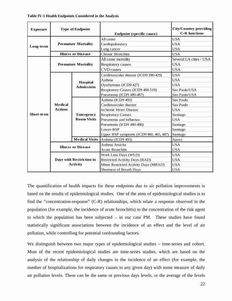
All the endpoints typically included in quantification analyses are represented in Table IV-1.

Also on the table are the cities and countries from which the concentration-response studies were

drawn. As the table shows, many, but not all, of these endpoints have been studied in Latin

American cities. Rather than ignoring these subsidiary endpoints, we treat them as separate

endpoints for calculation purposes and then net them out of the more inclusive endpoint cases or

values, as appropriate. In a next section we explain how this aggregation is performed.

16 By increasing degree of severity degree these endpoints are MRAD, RAD, WLD, so a WLD will be counted amongst the RADs and a RAD will also be counted in the MRADs,

22

Table IV-1 Health Endpoints Considered in the Analysis

ExposureEndpoint (specific cause)

City/Country providing C-R functions

All cause USACardiopulmonary USALung cancer USAChronic Bronchitis USAAll cause mortality Several LA cities / USARespiratory causes USACVD causes USACardiovascular disease (ICD9 390-429) USAAsthma USADysrhytmias (ICD9 427) USARespiratory Causes (ICD9 460-519) Sao Paulo/USAPneumonia (ICD9 480-487) Sao Paulo/USAAsthma (ICD9 493) Sao PauloCardiovascular disease Sao PauloIschemic Heart Disease USARespiratory Causes SantiagoPneumonia and Influenza USAPneumonia (ICD9 480-486) SantiagoLower-RSP SantiagoUpper RSP symptoms (ICD9 460, 465, 487) SantiagoAsthma (ICD9 493) JuarezAsthma Attacks USAAcute Bronchitis USAWork Loss Days (WLD) USARestricted Activity Days (RAD) USAMinor Restricted Activity Days (MRAD) USAShortness of Breath Days USA

Premature Mortality

Short-term

Illness or Disease

Days with Restriction in Activity

Medical Actions

Hospital Admissions

Emergency Room Visits

Medical Visits

Long-termPremature Mortality

Illness or Disease

Type of Endpoint

The quantification of health impacts for these endpoints due to air pollution improvements is

based on the results of epidemiological studies. One of the aims of epidemiological studies is to

find the ”concentration-response” (C-R) relationships, which relate a response observed in the

population (for example, the incidence of acute bronchitis) to the concentration of the risk agent

to which the population has been subjected – in our case PM. These studies have found

statistically significant associations between the incidence of an effect and the level of air

pollution, while controlling for potential confounding factors.

We distinguish between two major types of epidemiological studies – time-series and cohort.

Most of the recent epidemiological studies are time-series studies, which are based on the

analysis of the relationship of daily changes in the incidence of an effect (for example, the

number of hospitalizations for respiratory causes in any given day) with some measure of daily

air pollution levels. These can be the same or previous days levels, or the average of the levels

23

for some number of days before the event under study (for example, the average of the previous

three days). Confounders like ambient temperature, humidity, seasonal effects and the presence

of epidemics (like the flu epidemic) are controlled for in the analysis. Other potential

confounders, like the smoking habits of the population, are not supposed to change from day to

day in association with air pollution.

Due to its design, this type of study can only identify the effects that spikes in air pollution have

on health. They cannot pick up the cumulative effect of exposures over many years, for instance.

Nevertheless, these types of studies have been conducted all over the world, with populations of

different characteristics, health services provision, and meteorology (all factors that effect the

response of the population to air pollution). The result is a broad consensus that PM-10 has

significant effects on all of the endpoints noted in Table IV-1, although there are other endpoints,

(like the inception of asthma) where there is still not enough information.

Perhaps the most persuasive epidemiological studies, although far fewer in number, are the

cohort studies. This type of study follows a group of individuals (a cohort) for a relatively long

period of time (several years), recording the occurrence of health effects. The most important

characteristics of the individuals (body weight, smoking status, etc) can be assessed periodically,

so confounders are controlled by accounting for individual characteristics (such as smoking

history) Ambient characteristics (meteorology, air pollution) can be obtained from monitors

close to the individual’s residence. This kind of study is capable of assessing long-term effects of

air pollution on health, which, depending on design, may incorporate the short-term effects

picked up in time series studies. Because they are quite expensive to conduct, since they

required a long campaign of data collection, few of these studies have been done, all of them in

the US. Nevertheless, the cohort studies are those most often relied on in the U.S. in cost-

benefit analyses of air pollution regulations and are generally believed to be the most reliable and

comprehensive assessments of the long-term effects of PM-10 on health.

Details of Estimating Health Effects

Most of the C-R functions are of the relative risk type, i.e., they estimate the change in effects

relative to a baseline, which is usually the observed incidence of effects in the population of

analysis. The change in effects that a given population group experiences due to a change in

pollutant concentrations is therefore given as:

),,,( kkijij

kj

kij CIRPopfE ∆=∆ β

24

where

• kj

Pop is the number of people of group j that is exposed to the pollutant k

• ijIR is the incidence of endpoint i in population j

• kijβ is the unit risk of endpoint i in subpopulation j due to pollutant k

• kC∆ is the change in concentration of pollutant k

This can be rewritten as

( )[ ]kkijij

kij

kj

kij CIRIFPopfE ∆⋅=∆ ,),(, β

where ),( kijij

kij IRIF β is the impact factor of endpoint i in population group j due to pollution k,

which incorporates the unit risk jjβ and the incidence rate j

iIR of the effect.

It is important to note that effects are computed for a set of endpoints-subpopulation-pollutant

(i,j,k) , so before quantifying them we need to define:

the endpoints to be included in the analysis (i)

the subpopulations into which the population is to be separated. (j)

the pollutants included in the analysis (k)

Of course, the three decisions are related, since the impact of air pollution needs to have been

estimated before through epidemiological studies. Once pollutants are defined, we need to define

the endpoints, and that decision will condition our consideration of subpopulations.17 For

example, for acute bronchitis, the studies that have shown an association with PM10 have been

conducted only in children age 8-12 years.

Table IV-2 provides the number of studies for each endpoint and city in Latin America. Note

that Mexico City has been the most studied city in Latin America, with 10 studies to estimate

concentration-response functions, seven of which are for premature mortality. In total our

analysis uses up to 21 independent concentration-response functions taken from Latin American

17 There are many ways to disaggregate the population into different groups: by age, by gender, by health status, by educational level, and by socioeconomic status. All of these divisions have been shown, at least in one study in one place, to have different response to air pollution. The main division however is by age groups: Children, Adults, and Elderly. That is the division we use in this work.

25

efforts. These Latin American studies were obtained from a systematic review of the published

and unpublished literature, as well as the authors calling on their extensive academic network.

These studies are supplemented by a large number of studies from the U.S. and elsewhere.

Table IV-2 Number of health studies conducted in Latin American cities, by endpoint type

Morbidity City Premature Mortality Hospital

admissions Emergency Room Visits

Child Medical Visits

Mexico City 9 2 (1) 1 (2) Sao Paulo 4 3 1 Santiago 3 1 1 (3) Total 16 3 4 2 Notes (1) One study is for Ciudad Juarez (2) Child Medical Visits LRS (3) Child Medical Visits LRS, URS

In the next sections we assess the results of these studies.

IV.B Mortality impacts

The most severe impact is premature mortality. Also, it is the most studied and the most

important in terms of public welfare. Exposure to air pollution affects mortality rates in two

ways: an increase in pollution can have a short-term effect, increasing mortality over the days

following a spike in pollution. This is the kind of effect observed in the 1950’s and 60’s in

London, when a sharp increase in pollution lead to an increase of mortality rates in subsequent

days (Bell and Davis 2001). These effects are captured by the time-series studies noted above.

But constant exposure to air pollution can also have long-term effects: these are referred to as

“chronic” effects. These are the kind of effects uncovered by cohort studies. Cohort studies also

capture short-term effects.

IV.B.1 Time-Series Studies

By far, the most studied endpoint in Latin America is premature mortality associated with short-

term exposure to increased air pollution, i.e. changes in exposure in the previous days of the

death. All the studies are of the same type -- daily time series— which relate the average number

of deaths in a day with the air pollution levels in previous days.

26

Concentrations of ambient air pollutants, especially those that come from the same sources, are

usually highly correlated. Some studies attempt to separate the effects of different pollutants, by

simultaneously including them in the regression models. Since we are estimating the effects for

PM10, whenever possible we consider studies that include many pollutants simultaneously, which

is this case was only feasible for all ages. For elder, there were few studies with co-pollutants, so

we did not include them . Failing to control for ozone, for instance, would probably lead to an

overestimation of the PM effects, while controlling for more pollutants may result in an

underestimation, as some of the studies show.18

Since there are many studies of this endpoint, we conducted a “meta-analysis” – a statistical

analysis of multiple studies, where the results from each study are themselves treated as data and

conclusions about statistical relationships are made from considering these data across many

studies. Our meta-analysis included all the available studies in Latin America on each of the

endpoints where such studies existed. Studies were grouped by age groups (all ages, elderly

(>=65 yrs), and infants (less than 1 year old)) and by whether they considered any co-pollutants

in the statistical model. Summary estimates were obtained using a “fixed effects” model, in

which it is assumed that the results in each study are independent observations of the same

underlying process that differ only due to a statistical error, and using a “random effects” model,

in which it is assumed that the effect in each study has a fixed component plus a random

component, different for each study. Table IV-3 presents the summary estimates for the meta-

analyses of premature mortality coefficients for all ages and for the elderly.

18 With some notable exceptions like Castillejos 2000.

27

Table IV-3 Summary estimates from the Meta-analysis of Latin-American studies of the effects of PM10 on All Cause Mortality

Age group City Co-Pollutant Number of

studies Metric References

All AgesAll none 6 FE 0.41% ( 0.32% - 0.51% )

RE 0.61% ( 0.26% - 0.97% )

none 4 FE 0.70% ( 0.57% - 0.82% )

RE 0.87% ( 0.55% - 1.19% )

O3, SO2; O3 4 FE 0.43% ( 0.33% - 0.54% )

RE 0.91% ( 0.38% - 1.44% )

Mexico City none 3 FE 0.24% ( 0.09% - 0.38% )

RE 0.89% -( 0.05% - 1.85% )

O3, SO2; O3 2 FE 1.35% ( 0.89% - 1.82% )

RE 1.37% ( 0.85% - 1.89% )

Santiago none 2 FE 0.63% ( 0.49% - 0.76% )

RE 0.64% ( 0.47% - 0.80% )

O3 2 FE 0.38% ( 0.27% - 0.49% )

RE 0.55% ( 0.03% - 1.07% )

Elder 65+ yrAll None 5 FE 0.66% ( 0.51% - 0.81% )

RE 0.83% ( 0.48% - 1.17% )

O3, SO2; O3 3 FE 0.56% ( 0.37% - 0.75% )

RE 1.00% ( 0.24% - 1.77% )

México City O3, SO2; O3 2 FE 1.35% ( 0.76% - 1.95% )

RE 1.35% ( 0.76% - 1.95% )

Santiago None 2 FE 0.61% ( 0.44% - 0.78% )

RE 0.69% ( 0.30% - 1.08% )

Sao Paulo none 2 FE 0.71% ( 0.37% - 1.06% )

RE 0.81% ( 0.13% - 1.51% )

Infant < 18yrAll None 3 FE 2.73% ( 1.55% - 3.92% )

RE 2.94% ( 1.35% - 4.56% )

Sao Paulo None 2 FE 2.37% ( 1.05% - 3.72% )

RE 2.59% ( 0.54% - 4.69% )

O3, SO2; O3 2 FE 3.20% ( 1.29% - 5.16% )

RE 3.20% ( 1.29% - 5.16% )

Cifuentes 2000, Ostro 1996

Gouveia 2000b, Saldiva 1995

Castillejos 2000, Ostro 1996, Sanhueza 1998, Gouveia 2000b, Saldiva 1995

Borja-Aburto 1997, Castillejos 2000, Sanhueza 1998

Borja-Aburto 1997, Castillejos 2000

Ostro 1996, Sanhueza 1998

Loomis 1999, Linn 2000, Nishioka 2004

Loomis 1999, Nishioka 2004

Linn 2000, Nishioka 2004

% Increase per 10 ug/m3 PM10 (95% CI)

Borja-Aburto 1997, O'Neill 2004, Castillejos 2000, Cifuentes 2000, Ostro 1996, Gouveia 2000bBorja-Aburto 1997, Castillejos 2000, Cifuentes 2000, Ostro 1996

Borja-Aburto 1997, Castillejos 2000, Cifuentes 2000, Ostro 1996

Borja-Aburto 1997, O'Neill 2004-b, Castillejos 2000

Borja-Aburto 1997, Castillejos 2000

Cifuentes 2000, Ostro 1996

Note: FE = Fixed effects estimate, RE= Random Effects Estimate. Mid estimates shown in bold, 95% Confidence interval (percentile 2.5 to percentile 97.5 is shown in parenthesis)

The table shows that in almost all cases there is heterogeneity of impacts across cities that might

be due to several factors. Although all studies were conducted in urban areas with a population

over 5 million, cultural, socioeconomic, and demographic differences may influence the

28

susceptibility of the population. Population exposure may also vary from city to city since some

determinants of exposure , like concentration patterns and population mobility, might be

different. Data quality differences between cities may be another source of heterogeneity in the

studies. There is probably no quality problems in the meteorological data used for confounding

control, but there might be more variation in the way air pollution is measured and how health

data are colleted. Potential differences in diagnosis, recording, and reporting of health outcome

data may also introduce heterogeneity. Finally, although statistical methods used are similar (all

studies used Poisson regression), the way in which each research team adjusted for

meteorological and temporal factors may produce a difference. Since we have at most four cities

in any case, it is impossible to estimate the influence of each of these factors on the risk

coefficients.

For our analysis we use the random effects estimates. The summary estimate for all ages, all

cities yields an increase in mortality risk of 0.61% (0.26-0.97% )19 for an increase of 10 µg/m3 of

PM1020,21. Surprisingly, this risk increases to 0.91% (0.38-1.44%) when co-pollutants like O3

and SO2 are included in the statistical models. However, part of this increase occurs because

only 4 out of the 6 studies considered a co-pollutant; and for them the risk estimate without co-

pollutants is 0.87 (0.55-1.19)%. For the fixed effects model, the risk actually decreased from

0.70 (0.57-0.82)% to 0.43 (0.33-0.54)%. For the elderly, the situation is similar: the risk

increases from to 0.83(0.48-1.17)% to 1.00(0.24-1.77)%. In this case we cannot compare

outcomes of the studies, since there is only one study that has both estimates. As in the All ages

case, we choose to use the “no co-pollutant” estimate. This situation, in which the risk increases

when a co-pollutant is considered in the model, appears in other cases too. Since we do not want

to overestimate the effects, in those cases we choose to use so we use the estimates with no co-

pollutants.

The next table shows the estimates selected for each age group for all cities pooled together, and

for specific cities that had more than 2 estimates. As it is clear from the figure, the results are

19 The first number is the mid estimate, while the parenthesis shows the 95% Confidence interval (percentile 2.5 to percentile 97.5).

20 This means that for each 10 µg/m3 increase [decrease] in PM10 concentration, the number of deaths increases [decreases] 0.61%. This relative risk change is applied to the expected number of deaths to obtain the change in actual deaths associated to the change in PM10 concentrations.

21 This means that for each 10 µg/m3 increase [decrease] in PM10 concentration, the number of deaths increases [decreases] 0.61%. This relative risk change is applied to the expected number of deaths to obtain the change in actual deaths associated to the change in PM10 concentrations.

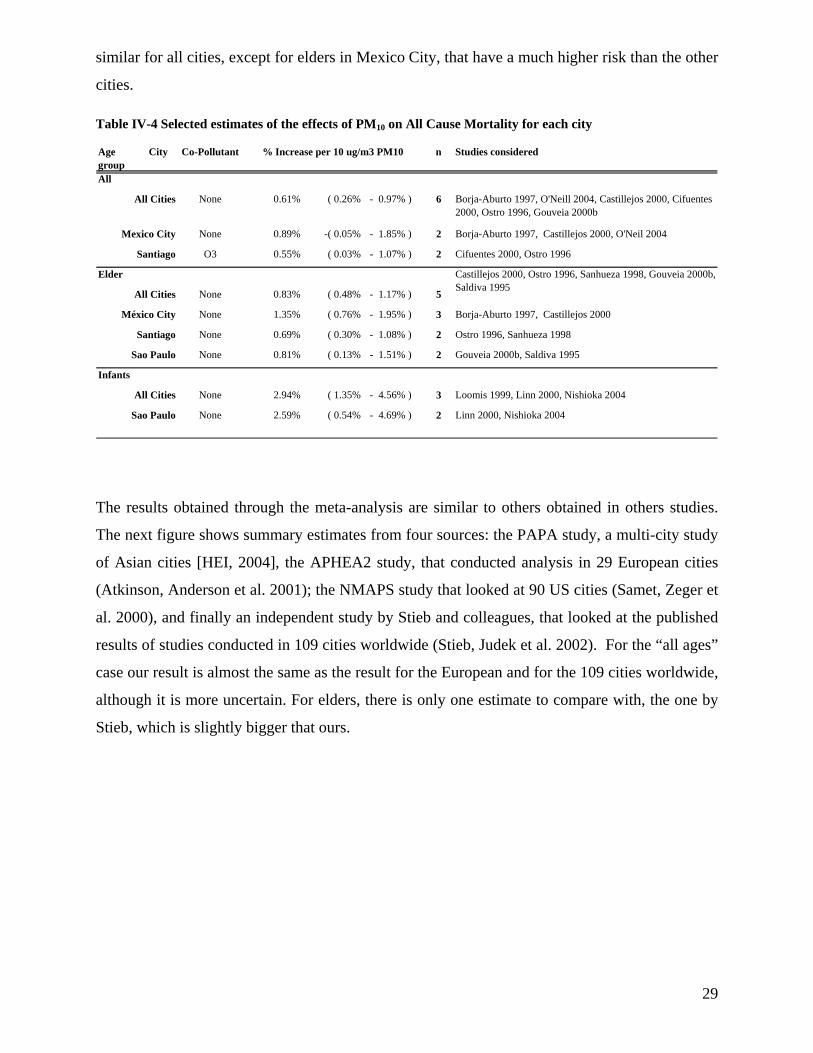
29

similar for all cities, except for elders in Mexico City, that have a much higher risk than the other

cities.

Table IV-4 Selected estimates of the effects of PM10 on All Cause Mortality for each city

Age group

City Co-Pollutant n Studies considered

All

All Cities None 0.61% ( 0.26% - 0.97% ) 6 Borja-Aburto 1997, O'Neill 2004, Castillejos 2000, Cifuentes 2000, Ostro 1996, Gouveia 2000b

Mexico City None 0.89% -( 0.05% - 1.85% ) 2 Borja-Aburto 1997, Castillejos 2000, O'Neil 2004

Santiago O3 0.55% ( 0.03% - 1.07% ) 2 Cifuentes 2000, Ostro 1996

Elder

All Cities None 0.83% ( 0.48% - 1.17% ) 5

México City None 1.35% ( 0.76% - 1.95% ) 3 Borja-Aburto 1997, Castillejos 2000

Santiago None 0.69% ( 0.30% - 1.08% ) 2 Ostro 1996, Sanhueza 1998

Sao Paulo None 0.81% ( 0.13% - 1.51% ) 2 Gouveia 2000b, Saldiva 1995

Infants

All Cities None 2.94% ( 1.35% - 4.56% ) 3 Loomis 1999, Linn 2000, Nishioka 2004

Sao Paulo None 2.59% ( 0.54% - 4.69% ) 2 Linn 2000, Nishioka 2004

% Increase per 10 ug/m3 PM10

Castillejos 2000, Ostro 1996, Sanhueza 1998, Gouveia 2000b, Saldiva 1995

The results obtained through the meta-analysis are similar to others obtained in others studies.

The next figure shows summary estimates from four sources: the PAPA study, a multi-city study

of Asian cities [HEI, 2004], the APHEA2 study, that conducted analysis in 29 European cities

(Atkinson, Anderson et al. 2001); the NMAPS study that looked at 90 US cities (Samet, Zeger et

al. 2000), and finally an independent study by Stieb and colleagues, that looked at the published

results of studies conducted in 109 cities worldwide (Stieb, Judek et al. 2002). For the “all ages”

case our result is almost the same as the result for the European and for the 109 cities worldwide,

although it is more uncertain. For elders, there is only one estimate to compare with, the one by

Stieb, which is slightly bigger that ours.

30

Figure IV-1 Comparison of summary results of the effects of PM10 on All Cause

IV.B.2 Mortality Impacts: Cohort Studies

No cohort study of the effects of PM has been conducted in Latin-America, and to our

knowledge, only four studies have been conducted worldwide to examine long term mortality,

three of them in the USA: the Harvard Six Cities study (Dockery, Pope III et al. 1993) , the

California Adventist Study (Abbey, Nishino et al. 1999) , and the so-called American Cancer

Society (ACS) Study (Pope III, Thun et al. 1995; Pope III, Burnett et al. 2002; Pope III, Burnett

et al. 2004). The only European study (Hoek et al, 2002) associated the risk of premature death

to proximity to major roads, so it is not applicable to this analysis.

Of the US studies, the ones by Pope and colleagues had the higher number of subjects considered

-- more than a half million people -- followed during a period of 17 years (1982 to 1998). It also

has the more sophisticated statistical analysis – including the consideration of both linear and

log-linear relative risk models22 --so we choose to use its estimates. Table IV-5 presents some of

the estimates from the cohort studies.

22 In a linear model, relative risk of death changes linearly with air pollution concentrations, while in a log-linear model, it changes with the log of the concentrations.

0.0%

0.5%

1.0%

1.5%

All C

ause M

ortality, All Ag

es ------

Papa

- 4 As

ian Cities

APHEA

2 - 2

9 Eu

ro Cities

NMMAP

S - 9

0 US cities

Stieb et al 200

0 - 1

09 studies

worldwide Th

is study

All C

ause M

ortality, Elder -------

Stieb et al 200

0 - 1

09 studies

worldwide Th

is study

31

Table IV-5 Risk estimates reported in the studies of the long-term exposure to particulate matter explain entries – central & confidence interval

Age Group Cohort C-R Specif.

Exposure metric Source

All Cause mortality6 US cities >24 8,192 Linear Avg PM2.5 13.2% ( 4.1% - 23.1% ) Dockery, Pope III et al. 1993151 US cities (ACS cohort)

>30 552,138 adults

Linear Median PM2.55.7% ( 1.5% - 10.0% )

Pope III, Thun et al. 1995

California, USA >27 6,338 non smoking

Linear Avg PM100.1% ( 0.1% - 0.1% )

Abbey, Nishino et al. 1999

Cardio-pulmonary mortality151 US cities (ACS cohort)

> 30 552,138 adults

Linear Avg. 79-83PM2.5

5.9% ( 1.5% - 10.5% )Pope III, Burnett et al. 2002

Avg PM2.5 9.3% ( 3.3% - 15.8% )Log-Linear

Avg. 79-83PM2.5

1.2% ( 0.3% - 2.0% )Cohen, Anderson et al.

Avg PM2.5 1.6% ( 0.6% - 2.5% )

Lung cancer mortality151 US cities (ACS cohort)

> 30 552,138 adults

Linear Avg. 79-83PM2.5

8.2% ( 1.1% - 15.8% )Pope III, Burnett et al. 2002

Avg PM2.5 13.5% ( 4.4% - 23.4% )Log-Linear

Avg. 79-83PM2.5

1.7% ( 0.3% - 3.1% )Cohen, Anderson et al. 2004

Avg PM2.5 2.3% ( 0.9% - 3.8% )(*) For linear CR the PM2,5 change considered is 10 ug/m3. For the log-linear CR, the change considered is 10%

For example, if PM2.5 decreases 20%, the % change in lung cancer mortality, based on average PM2.5 (last line), equals -4.6% ( 2.3 *(-20%/10%))

Cause Location % change in deaths for given change in PM2.5 (*)

The use of the US studies in a Latin American context should be undertaken with extreme care.

First, the age structure of the population, as well as the underlying causes of death, can be quite

different and must be factored into the analysis. For instance, a country with many more young

people as a fraction of the total population will not only have a lower baseline death rate but will

also appear to be less susceptible to air pollution when looking over the entire population.

Looked at another way, a country with few elderly people, say because they die from non-air

pollution causes before they become elderly, will appear less susceptible than more elderly. We

were not able to directly adjust for this age effect. However, to address the differences in causes

of death, we estimated excess deaths from a) all causes, using the results from Pope et al 1995,

and b) from cardiopulmonary causes and lung cancer using the results from Pope et al 2002.

We added these latter two and compared them to the all cause estimates, choosing the bigger

estimate of excess deaths. The second issue is the relationship of PM10 to PM2.5 in the cities

under analysis. We generally do not have PM2.5 data for LAC. To apply the linear PM2.5 model

with PM10 concentrations we assumed, in the base case, a ratio of PM2.5 to PM10 of 0.50. (Bogo,

Otero et al. 2003) (Jorquera 2002). This ratio is somewhat lower than the usual one assumed by

the USEPA for the USA for example, but the data in LAC shows that the crustal content in PM10

may be higher than that in the US. For example, in Santiago, the ratio of monthly data from 1995

to 2001 is 0.47. Had we used the higher ratio, the estimated deaths averted from reducing PM

32

would have been larger, .23 For the log-linear model using PM2.5 data estimates, we assumed that

the relative change in PM2.5 concentrations is the same as the relative change in PM10

concentrations. This might be an underestimation if control measures are aimed at reducing

combustion related to PM10. If control measures are aimed at controlling crustal material

(resuspended dust from roads, for example), then this assumption is an overestimation, since the

relative decrease in PM2.5 concentrations will be smaller than the relative decrease for PM10.

The final issue is the difference in PM-10 concentrations between U.S. and Latin American

cities. Simply put, air quality in U.S. cities is generally better than in LA cities. The average

concentrations in the cities used in the ACS study range from 15 to 25 µg/m3 of PM2.5, which

corresponds to approximately 30 to 50 µg/m3 of PM10 , using the ratio assumed above. Many of

the Latin American cities are in the 60 to 80 ug/m3 range, or even higher.

In extrapolating the US results outside of its original range the shape of the C-R function is

critical. While the two functions considered – linear and log-linear – do not differ significantly

within the range of the original study, their estimates are quite different when applied to

concentrations well outside it, like the ones found in LAC. Since there is evidence that the C-R

function is downward sloping, we chose to use the log-linear specification proposed by Cohen et

al 2004 for cardio-pulmonary and lung-cancer mortality instead of the linear specification for all

cause mortality.24

IV.B.3 Summary - Comparison of time-series and cohort coefficients

How do the time-series and cohort coefficients compare? Figure IV-1 shows the concentration

response functions for different mortality endpoints, using the case of Buenos Aires for

illustration. The curves are anchored at the reference level of 50 µg/m3. For example, for

Buenos Aires attaining the standard implies a reduction of 60 µg/m3 (from 110 µg/m3 to 50

µg/m3 PM10), or 45%. Mortality risk decreases 3.6% due to the effects of short-tem exposure to

air pollution (as taken from time-series studies), while for long-term effects it decreases 27% for

23 There is another, more technical, issue. The Pope et al and Cohen et al estimates are based on three PM metrics: the average of 5 years (1979-83: mean PM2.5 = 21 µg/m3 ), the average of 1999-2000 (mean PM2.5 = 14) and on the average of both (mean PM2.5 = 17 µg/m3 ). We used the estimates from the third measure since they include more types of concentration patterns, thereby reducing differences in concentration patterns between LA and the U.S.

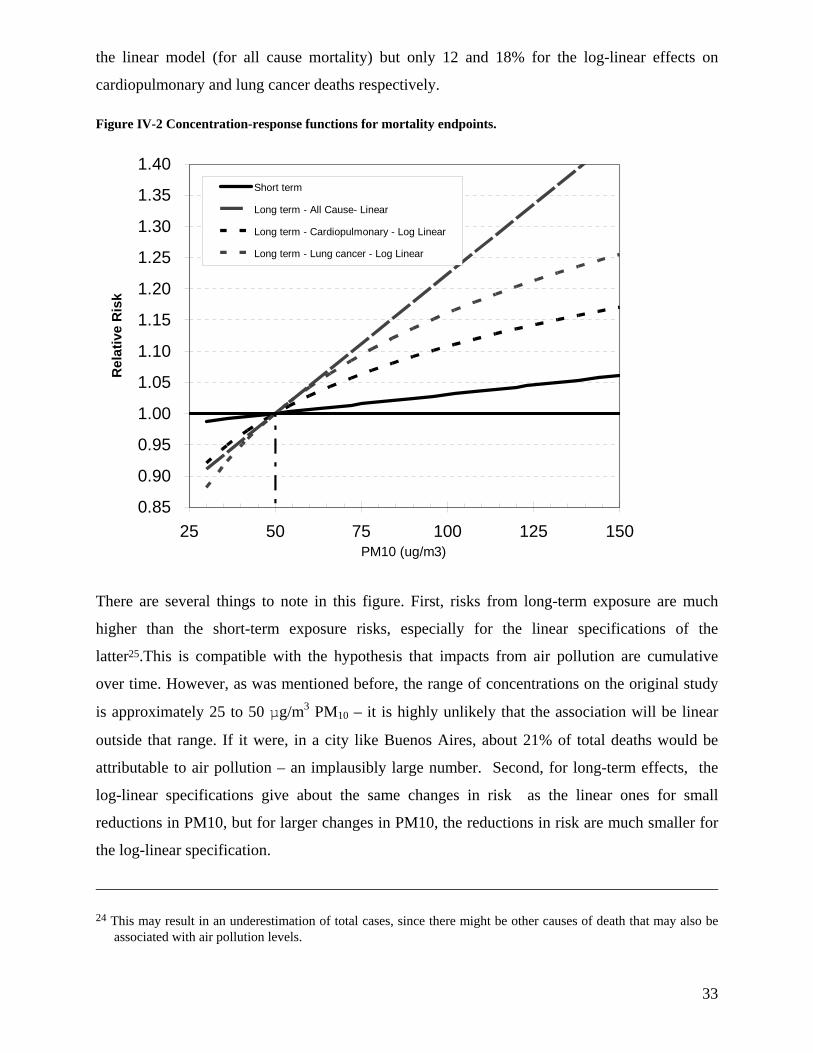
33

the linear model (for all cause mortality) but only 12 and 18% for the log-linear effects on

cardiopulmonary and lung cancer deaths respectively.

Figure IV-2 Concentration-response functions for mortality endpoints.

0.85

0.90

0.95

1.00

1.05

1.10

1.15

1.20

1.25

1.30

1.35

1.40

25 50 75 100 125 150PM10 (ug/m3)

Rel

ativ

e R

isk

Short term

Long term - All Cause- Linear

Long term - Cardiopulmonary - Log Linear

Long term - Lung cancer - Log Linear

There are several things to note in this figure. First, risks from long-term exposure are much

higher than the short-term exposure risks, especially for the linear specifications of the

latter25.This is compatible with the hypothesis that impacts from air pollution are cumulative

over time. However, as was mentioned before, the range of concentrations on the original study

is approximately 25 to 50 µg/m3 PM10 – it is highly unlikely that the association will be linear

outside that range. If it were, in a city like Buenos Aires, about 21% of total deaths would be

attributable to air pollution – an implausibly large number. Second, for long-term effects, the

log-linear specifications give about the same changes in risk as the linear ones for small

reductions in PM10, but for larger changes in PM10, the reductions in risk are much smaller for

the log-linear specification.

24 This may result in an underestimation of total cases, since there might be other causes of death that may also be associated with air pollution levels.

34

IV.C Morbidity impacts

IV.C.1 Latin American Studies

As shown above, fewer studies of morbidity effects have been conducted in Latin America than

for mortality effects, and the former have focused only on hospital admissions, emergency room

visits, and child medical visits. Most of the studies have been conducted for children, in Sao

Paulo, Brazil, as Figure IV-2 shows. All the studies refer to medical actions, from hospital

admissions to medical visits, and except for one study (Lin, Amador Pereira et al. 2003) all focus

on respiratory related endpoints. The figure shows the estimated percent change in the listed

endpoint per 10ug/m3 change in PM10 and also provides uncertainty bounds for these

coefficients encompassing the 95% confidence interval ( 2.5th and 97.5th percentile).

Figure IV-2 shows the mid estimate and the confidence interval for all the endpoints studied.

The higher risks correspond to emergency room visits related to general respiratory causes. Next

come hospital admissions, also for general respiratory causes. The risk to children and the elderly

is almost the same, according to the estimates from three Brazilian studies.26 Risks for more

specific causes are smaller.

25 It should be noted that the long-term exposure risks are applied to the population older than 30 years. However, most of the deaths in the total population are for people 30 or older, so the estimates are comparable.

26 Although there are only 3 studies, we have 8 estimates due to two reasons: these studies present results for several sub-age groups within the less than 18 year old bracket, so we lump them together, and one study was performed in Sao Paulo and Rio de Janeiro

35

Figure IV-2. Percentage increase in baseline effects per 10µg/m3 of PM10 for morbidity endpoints in Latin-American studies

Note: bars indicate the 95% confidence interval

IV.C.2 USA Studies

Although the Latin American studies cover several morbidity endpoints, some important ones,

especially for WTP, are missing. We complemented the LAC studies with some North-

American based studies, used by the US EPA in their Regulatory Impact Analyses (EPA 1997,

EPA 1999). The selection from the huge array of studies available aimed to cover some

underrepresented endpoints (like all the symptoms and restriction in activity effects) and was

conditioned by the availability of incidence rate data.

0%1%

2%3%

4%5%

Hospital Admissions ----------------

Respiratory (ICD 460-519) Children Sao Paulo

Elder Sao Paulo

Pneumonia (ICD 480-487) Children Sao Paulo

Asthma (ICD 493) Children Sao Paulo

Emergency Room Visits ---------------

Asthma (ICD 493) Children Ciudad Juarez

Respiratory Children Santiago

Sao Paulo

Pooled

Cardiovascular All Sao Paulo

Pneumonia (ICD 48 0-486) Children Santiago

Upper respiratory symptons (ICD 460, 465, 487) Children

Santiago

Pooled

Medical Visits ---------------

Lower respiratory symptoms Children México DF

Santiago

Upper respiratory symptoms Children Santiago

36

Table IV-6 Summary of morbidity risk estimates for studies conducted in North American cities

Age group Co-Pollutant Reference

Hospital Admissions

All none linear model Thurston 1994none 1.7% ( 0.9% - 2.5% ) PooledO3 2.3% -( 0.6% - 5.2% ) Schwartz 1995none 2.1% ( 0.9% - 3.3% ) Burnett 1997O3 0.3% -( 1.2% - 1.8% ) Burnett 1997

COPD (ICD 490-496) Elder none 2.6% ( 1.8% - 3.5% ) PooledAll none 2.7% ( 1.8% - 3.6% ) Burnett 1999

Elder none 1.3% ( 0.8% - 1.9% ) PooledAdult none 2.6% ( 1.1% - 4.2% ) Sheppard 1999

Children none 2.6% ( 1.1% - 4.2% ) Sheppard 1999none 2.3% ( 0.3% - 4.4% ) Burnett 1997O3 1.7% -( 0.3% - 3.8% ) Burnett 1997

Elder none 1.2% ( 1.0% - 1.4% ) Samet 2000Dysrhythmia (ICD 427) All none 1.6% ( 0.6% - 2.7% ) Burnett 1999

Emergency Room VisitsAdult none 3.7% ( 1.2% - 6.3% ) Schwartz 1993

Children none 12.0% ( 9.2% - 14.8% ) Norris 1999

Illness & SymptomsAcute Bronchitis Children none 16.1% -( 3.4% - 39.6% ) Dockery et al. 1996Asthma Attacks All O3 1.5% ( 0.4% - 2.6% ) Whittemore 1980

Shortness of Breath (days) Children none 18.3% ( 2.6% - 36.4% ) Ostro 1995Restriction in Activity

Work loss days (WLDs) Adult none 5.2% ( 4.4% - 6.0% ) Ostro 1987Restricted Activity Days Adult none 2.6% ( 2.3% - 3.0% ) Ostro 1987

Minor Rest. Act. Days Adult none 4.2% ( 3.4% - 5.0% ) Ostro 1989

% Increase per 10 ug/m3 PM10Endpoint

Elder

All

Asthma (ICD 493)

Respiratory Causes (ICD 460-519)

Cardiovascular disease (ICD 390-429)

All

Pneumonia (ICD 480-487)

Asthma (ICD 493)

37

V. Health Valuation

As noted in Section I, the monetary value of health improvements can be estimated in two broad

ways: (i) through measures of monetary outlays and forgone wage compensation – termed the

cost-of-illness (COI) approach, and (ii) through measures of what individuals would be willing to

give up to obtain health improvements, e.g., willingness to pay (WTP). In this section we

present a brief introduction to each method and then discuss the values used in this study.

V.A Values used in the Analysis

For a complete analysis it is necessary to have a value attached to each health effect whose

change can be estimated. Ideally, WTP values are the best approximation to the welfare effects

deriving from improving air quality. Unfortunately, these values are not generally available so

COI estimates are generally used. Another option is transferring values (WTP or COI) from

other contexts, as we have done by rescaling USA unit values to apply in a LAC context. In this

section we present the values used in this study, which are from both COI and WTP studies.

V.A.1 Available unit values from Latin America and the US

Unit values have been collected from analyses conducted in the US and Europe. But we would

prefer to use local values where possible. To that end, we conducted a bibliography search

looking for values for health effects in Latin America studies. The main source of data were

previous benefit analyses conducted in the region, mainly in Sao Paulo, Mexico City, and

Santiago, and also in Buenos Aires, where a study (Conte-Grand 2002) has estimated the co-

benefits of GHG mitigation.27 Table V-1 shows the unit medical costs available for Latin

American cities and for the US, while Table V-2 shows the WTP unit values.

The unit medical costs, which one would expect to be more or less in line across countries of a

similar level of development, show a wide variation. The values from Holz (Holz 2000) are

generally the smaller ones. This might be because those values are derived from epidemiological

profiles that are then valued at market prices. Many indirect costs may have not been considered

27 This study is interesting in the sense that although there are no local epidemiology studies available in Argentina, it develops unit values for some endpoints estimated using transferred value functions.

38

in that valuation. The most striking dissimilarities come from the two Mexican studies. The

McKinley et al study has much bigger values than the Cesar et al. study. McKinley et al

considered costs from the health provider (IMSS – Mexican Institute of Social Security)

perspective, valuing the highest level of hospitalization for some diseases, which included

intensive care unit costs plus attention from staff in the room. In contrast, Cesar et al used the

results of a previous study (Hernandez-Avila and al 1995) that was not available for our review.

The most striking difference is for chronic bronchitis, where the values differ by a factor of 80

(US$218 vs. $17,750 per case). The Buenos Aires values for medical costs, from Conte Grande

2002, generally fall between these values.

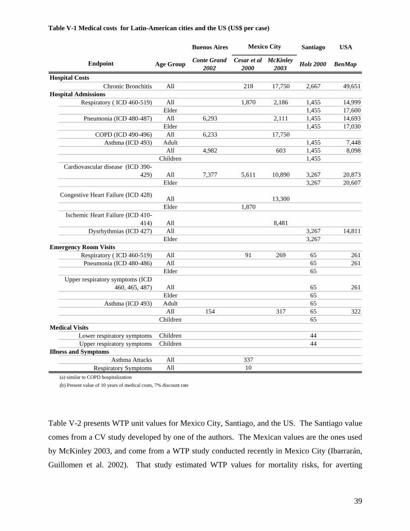
39

Table V-1 Medical costs for Latin-American cities and the US (US$ per case)

Buenos Aires Santiago USA

Age Group Conte Grand 2002

Cesar et al 2000

McKinley 2003 Holz 2000 BenMap

Hospital CostsChronic Bronchitis All 218 17,750 2,667 49,651

Hospital AdmissionsRespiratory ( ICD 460-519) All 1,870 2,186 1,455 14,999

Elder 1,455 17,600Pneumonia (ICD 480-487) All 6,293 2,111 1,455 14,693

Elder 1,455 17,030COPD (ICD 490-496) All 6,233 17,750

Asthma (ICD 493) Adult 1,455 7,448All 4,982 603 1,455 8,098

Children 1,455Cardiovascular disease (ICD 390-

429) All 7,377 5,611 10,890 3,267 20,873Elder 3,267 20,607

Congestive Heart Failure (ICD 428) All 13,300Elder 1,870

Ischemic Heart Failure (ICD 410-414) All 8,481

Dysrhythmias (ICD 427) All 3,267 14,811Elder 3,267

Emergency Room VisitsRespiratory ( ICD 460-519) All 91 269 65 261 Pneumonia (ICD 480-486) All 65 261

Elder 65Upper respiratory symptoms (ICD

460, 465, 487) All 65 261Elder 65

Asthma (ICD 493) Adult 65All 154 317 65 322

Children 65Medical Visits

Lower respiratory symptoms Children 44Upper respiratory symptoms Children 44

Illness and SymptomsAsthma Attacks All 337

Respiratory Symptoms All 10(a) similar to COPD hospitalization(b) Present value of 10 years of medical costs, 7% discount rate

Endpoint

Mexico City

Table V-2 presents WTP unit values for Mexico City, Santiago, and the US. The Santiago value

comes from a CV study developed by one of the authors. The Mexican values are the ones used

by McKinley 2003, and come from a WTP study conducted recently in Mexico City (Ibarrarán,

Guillomen et al. 2002). That study estimated WTP values for mortality risks, for averting

40

chronic bronchitis, and averting a cold. The values presented in the table are the values from the

WTP study.

Table V-2 Unit WTP values for Latin American Cities and for the US studies ($/case)

Santiago USACesar et al

2000McKinley 2003

(*) Cifuentes 2000 BenMap

Reductions in Risk of DeathStatistical Life All 506,000 634,000 6,240,000

Chronic IllnessChronic Bronchitis All 118,074 28,000 340,000

Hospital AdmissionsPneumonia (ICD 480-487) All 153 330

COPD (ICD 490-496) All 153 330Asthma (ICD 493) All 153 330

CVD (ICD 390-429) All 153 330Congestive Heart Failure (ICD 428) All 153 330chemic Heart Failure (ICD 410-414) All 153 330Emergency Room Visits

Respiratory ( ICD 460-519) All 79 170 Asthma (ICD 493) All 79 170

IllnessAsthma Attacks Adult 15 43.0

Restriction in ActivityRestricted Activity Days All 98.0

Minor Restricted Activity Days Adult 21 20 50.5

(*) The VSL comes from Ibarrarán, Guillomen et al 2002

Endpoint Age GroupMexico City

The Mexican studies have data only for Minor RADs. Since there are US data for both MRADs

and RADs, we computed a LA based unit value for RADs based on the Mexican MRAD value

multiplied by the ratio of US values for RADs and MRADs (98/50.5)

V.A.2 Transference of WTP Values

As should be apparent from the previous tables, many Latin American cities do not have any

locally estimated values, and for many endpoints there are no Latin American values at all. In

this case it is possible to “transfer” values from other cities or countries, using the following

equation:

η

⎟⎟⎠

⎞⎜⎜⎝

⎛=

SourceSource PCI

PCIUVUV Target

Target

where η is the income elasticity of demand for health. The underlying hypothesis in the benefit

transfer approach is that valuation differences can be explained primarily by income differences.

41

An elasticity of 1 would mean that the transferred WTP would be proportional to income

differences, while a value of 0 would mean that demand for health is not dependent on income,

so the values for the target and source cities should be the same. WTP studies have estimated

income elasticities from 0.2 to greater than two (Alberini, Cropper et al. 1997; Bowland and

Beghin 2001).

The selection of the way to transfer values (both the metric of income considered and the value

of the transfer elasticity) and the source of the original values can produce big differences in the

transferred values. For premature mortality, which is the effect whose reduction can produce the

biggest benefits, we choose to use the average of the two studies available in LA, adjusting them

by per-capita income (PCI) with an elasticity of 1. This elasticity, rather than 0.4, was used

because of the similar development patterns of countries in LA compared to that of the U.S.. The

Ibarrarán et al 2002 study yields a ratio with respect to the PCI of 64, while the Cifuentes et al

2000 study yields a ratio of 128. For other cities in Latin America, we use the average ratio of

VSL to PCI of 96.5 to compute the VSL for all other cities. We also transferred the USA value

(US$ 6.24 million per case in 2000 dollars) using the ratio of the purchasing power parity

income (PPPI), with a transfer elasticity of 0.4 (Alberini, Cropper et al. 1997; Bowland and

Beghin 2001). The transferred values for each city are shown in Table V-3.

The table shows than the values transferred from the USA are much higher than the ones

transferred from Mexico and Santiago. This can be explained by three factors: i) The original US

value is higher than the Mexico and Santiago values (the ratio with respect to for the US PCI is

178 for the US value, compared to an average of 97 for LAC.), ii) The relative differences in

PPPI are lower than the relative differences in PCI – in other words, the income ratio is closer to

1 in the formula above with PPPI., iii) The use of an elasticity of 0.4 instead of 1.0 tends to make

the income differences even less significant in transferring the US unit values

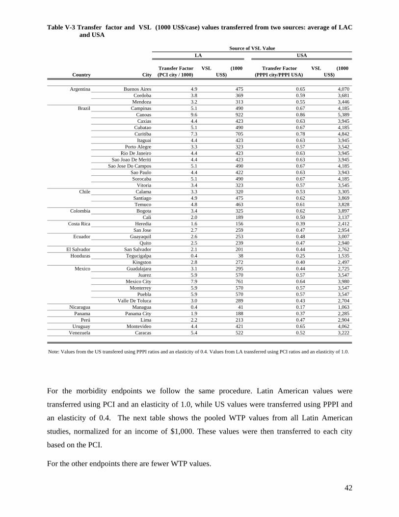
42

Table V-3 Transfer factor and VSL (1000 US$/case) values transferred from two sources: average of LAC and USA

Country City Transfer Factor (PCI city / 1000)

VSL (1000 US$)

Transfer Factor (PPPI city/PPPI USA)

VSL (1000 US$)

Argentina Buenos Aires 4.9 475 0.65 4,070 Cordoba 3.8 369 0.59 3,681

Mendoza 3.2 313 0.55 3,446 Brazil Campinas 5.1 490 0.67 4,185

Canoas 9.6 922 0.86 5,389 Caxias 4.4 423 0.63 3,945

Cubatao 5.1 490 0.67 4,185 Curitiba 7.3 705 0.78 4,842 Itaguai 4.4 423 0.63 3,945

Porto Alegre 3.3 323 0.57 3,542 Rio De Janeiro 4.4 423 0.63 3,945

Sao Joao De Meriti 4.4 423 0.63 3,945 Sao Jose Do Campos 5.1 490 0.67 4,185

Sao Paulo 4.4 422 0.63 3,943 Sorocaba 5.1 490 0.67 4,185

Vitoria 3.4 323 0.57 3,545 Chile Calama 3.3 320 0.53 3,305

Santiago 4.9 475 0.62 3,869 Temuco 4.8 463 0.61 3,828

Colombia Bogota 3.4 325 0.62 3,897 Cali 2.0 189 0.50 3,137

Costa Rica Heredia 1.6 156 0.39 2,412 San Jose 2.7 259 0.47 2,954

Ecuador Guayaquil 2.6 253 0.48 3,007 Quito 2.5 239 0.47 2,940

El Salvador San Salvador 2.1 201 0.44 2,762 Honduras Tegucigalpa 0.4 38 0.25 1,535

Kingston 2.8 272 0.40 2,497 Mexico Guadalajara 3.1 295 0.44 2,725

Juarez 5.9 570 0.57 3,547 Mexico City 7.9 761 0.64 3,980

Monterrey 5.9 570 0.57 3,547 Puebla 5.9 570 0.57 3,547

Valle De Toluca 3.0 289 0.43 2,704 Nicaragua Managua 0.4 41 0.17 1,063

Panama Panama City 1.9 188 0.37 2,285 Perú Lima 2.2 213 0.47 2,904

Uruguay Montevideo 4.4 421 0.65 4,062 Venezuela Caracas 5.4 522 0.52 3,222

Source of VSL ValueLA USA

Note: Values from the US transfered using PPPI ratios and an elasticity of 0.4. Values from LA transferred using PCI ratios and an elasticity of 1.0.

For the morbidity endpoints we follow the same procedure. Latin American values were

transferred using PCI and an elasticity of 1.0, while US values were transferred using PPPI and

an elasticity of 0.4. The next table shows the pooled WTP values from all Latin American

studies, normalized for an income of $1,000. These values were then transferred to each city

based on the PCI.

For the other endpoints there are fewer WTP values.

43

Table V-4 Pooled unit values from LAC WTP studies (US$ per 1000 $PCI)

Endpoint Age Group Latin-American Studies Mid Number of

studies Range

Reductions in Risk of Death Statistical Life All 96,465 2 64,172 to 128,757

Chronic Illness Chronic Bronchitis All 9,263 2 3,551 to 14,975

Hospital Admissions Pneumonia (ICD 480-487) All 30.6 2 19 to 42 COPD (ICD 490-496) All 30.6 2 19 to 42 Asthma (ICD 493) All 30.6 2 19 to 42 CVD (ICD 390-429) All 30.6 2 19 to 42 Congestive Heart Failure (ICD 428) All 30.6 2 19 to 42 Ischemic Heart Failure (ICD 410-414) All 30.6 2 19 to 42

Emergency Room Visits Respiratory ( ICD 460-519) All 15.8 2 10 to 22 Asthma (ICD 493) All 15.8 2 10 to 22

Illness Asthma Attacks Adult 1.9 1 -

Restriction in Activity Restricted Activity Days All 5.0 extrap. - Minor Restricted Activity Days Adult 2.6 2 2.54 to 2.66

Table V-5 shows, as an illustration, the transferred WTP values for two cities,: a high income

city (Curitiba, Brazil: PCI=7,309; PPPI=18,595) and a much poorer city (Panama City: PCI=

1,949; PPPI=2,846). The table illustrates the dependence of the transferred WTP values on

income, with the Curitiba values being several times the ones for Panama City. It also shows that

the relative difference is smaller for the USA transferred values, because of the value of the

transfer elasticity.

44

Table V-5 Transferred WTP unit values to for two cities, Curitiba and Panama City (US$ per case)

LA LAEndpoint All All Children Adult All All Children Adult

Chronic Bronchitis 67,703 263,812 18,054 124,521

Hosp Adm CVD (ICD 390-429) 226.6 60

Hosp Adm Pneumonia (ICD 480-487) 226.6 60

Hosp Adm Asthma (ICD 493) 226.6 60

ERV RSP 116.9 31.18

ERV Asthma (ICD 493) 116.9 31.18

Child Medical Visits LRS 25.2 11.9

Child Medical Visits URS 22.1 10.44

Acute Bronchitis 276.2 130.38

Asthma Attacks 14.6 33.4 33.4 3.9 15.75 15.75

Restricted Activity Days (RADs) 36.6 9.75

Minor Restricted Activity Days (MRADs) 21.9 57.4 5.85 27.1

Acute Morbidity any of 19 respiratory symptoms 18.6 8.79

Shortness of Breath (days) 4.7 4.7 2.2 2.2

Work loss days (WLDs)

Curitiba, Brazil

USA

Panama City, Panamá

USA

Note: values transferred using a) PCI ratios and a elasticity of 1.0 for LA, and b) PPPI ratios and a elasticity of 0.4 for USA

V.A.3 Transference of Medical Costs

Data for medical costs were available from three cities in LAC, plus the US. To apply them to

cities of other countries, we need to adjust them, not by an income indicator as in the WTP case,

but by a cost indicator. The best indicator to transfer medical costs would be an indicator based

on the unit costs of medical procedures in each country. Unfortunately, to our knowledge, such

an indicator is not available. The closest one, the per capita health expenditure statistics 28 from

the World Health Organization, reflects total expenditure per person, which is not applicable

because of the different health service coverage and age structure of the population, among other

factors.

Due to the lack of a better indicator, we choose to use per-capita income. Of course this is an

imperfect transfer indicator for this case, since costs of medical procedures are impacted by

28 See Who National Health Accounts (http://www.who.int/nha/en )

45

several factors not considered in income. 29 We tried per-capita income and purchasing power

parity income, comparing the unit costs for endpoints (i.e. costs normalized per $1000 of

income) for those endpoints that had estimates for the three countries plus the US several

countries. The comparison shows that costs normalized using the PPPI are more similar across

countries than those normalized using PCI30.is a better indicator. Therefore, we chose to use

PPPI as a basis for transferring the medical costs. Table V-6 shows the pooled medical cost

estimates from all Latin American studies, normalized for a PPPI of $1,000.

29 For example, the cost of imported resources, which may be important in many procedures, is not related to per-capita income.

30 This comparison implies that we should use a transfer elasticity of 1.0. The number of observations for each endpoint prevent us from testing a different elasticity.

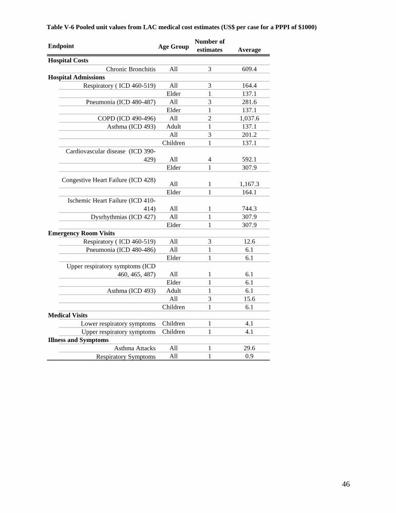
46

Table V-6 Pooled unit values from LAC medical cost estimates (US$ per case for a PPPI of $1000)

Age GroupNumber of estimates Average

Hospital CostsChronic Bronchitis All 3 609.4

Hospital AdmissionsRespiratory ( ICD 460-519) All 3 164.4

Elder 1 137.1Pneumonia (ICD 480-487) All 3 281.6

Elder 1 137.1COPD (ICD 490-496) All 2 1,037.6

Asthma (ICD 493) Adult 1 137.1All 3 201.2

Children 1 137.1Cardiovascular disease (ICD 390-

429) All 4 592.1Elder 1 307.9

Congestive Heart Failure (ICD 428) All 1 1,167.3Elder 1 164.1

Ischemic Heart Failure (ICD 410-414) All 1 744.3

Dysrhythmias (ICD 427) All 1 307.9Elder 1 307.9

Emergency Room VisitsRespiratory ( ICD 460-519) All 3 12.6 Pneumonia (ICD 480-486) All 1 6.1

Elder 1 6.1Upper respiratory symptoms (ICD

460, 465, 487) All 1 6.1Elder 1 6.1

Asthma (ICD 493) Adult 1 6.1All 3 15.6

Children 1 6.1Medical Visits

Lower respiratory symptoms Children 1 4.1Upper respiratory symptoms Children 1 4.1

Illness and SymptomsAsthma Attacks All 1 29.6

Respiratory Symptoms All 1 0.9

Endpoint

47

V.A.4 Lost Productivity values

Lost productivity values are computed from the average days lost due to occurrence of a case

times the average daily wage for the city. Income figures are readily available. For the duration

of the effects, we relied on data from Mexico City and from Santiago, as shown in Table V-7.

It should be noted that these are only days spent in the hospital (except for chronic bronchitis, for

which a duration of 10 years is assumed). Probably individuals who spent time at the hospital

will require a period of convalescence, increasing their productivity loss. These data are not

available from hospital admission records. For the calculations we estimated that the individual

requires a convalescence period of half the time spent in the hospital.

Table V-7 Average Length of stay for hospital admissions (days per case)

Endpoint All Children Adult ElderIntensive Care Unit

Hospital days

Chronic Bronchitis 10yr 10yrHospital Admissions

CVD (ICD 390-429) 8.4 8.1 8.2 9.3 Congestive Heart Failure 5 7

AMI 7 15 Dysrhythmias (ICD 427) 6.8 6.8 9.3

RSP (ICD 460-519) 8.8 8.2 8.9 9.0 Pneumonia (ICD 480-487) 6.9 6.9 11.6 7

Asthma (ICD 493) 6.8 5.3 7.3 6.7 2 COPD 10 15

(*) Corresponds to total disability period, not only hospital staySources:

México City: values from the IMSS reported in McKinley 2003

Santiago: averages from the whole country, from the 1996 Hospital Discharges database from the Ministry of Health computed in Cifuentes, 2001.

México CitySantiago

We assumed that in the case of children and the elderly, an adult will take care of them for some

fraction of the time. For children, we assumed 50% of the time spent by an adult. For the

elderly, we assumed 25%.

48

We value these effects at an average daily wage, computed as the annual per-capita income

divided by 365 days, since the illness can affect both workdays and holidays, and both employed

and unemployed people31.

To value the days of lost work estimated directly from the corresponding CR function we used

the average daily wage of the employed population. The average daily wage was computed as

the annual per-capita income divided by 260 workdays per year (assuming holidays are valued at

the same rate) and by the fraction of the employed population. Unemployment rates for urban

areas were obtained from the Statistical Yearbook of ECLAC (ECLAC 2002)

VI. Scenario Definition and Analysis Strategy

Scenarios were developed for the magnitude of the ambient concentrations reduction (Pollution

Reduction scenarios), for the quantification of the health effects given a change in concentrations

(Health scenarios), and for the unit values used to monetize these effects (Valuation scenarios).

To address the uncertainties present at many points in the analysis, we analyzed alternative

scenarios where the uncertainties couldn’t be characterized by statistical uncertainty but reflected

discrete options for modeling.

VI.A Pollution reduction scenarios

Since we did not analyze a specific set of pollution reduction measures, we choose to analyze

two scenarios that represent what we called ‘canonical’ cases of pollution reductions.

Because all the recent scientific evidence shows that there is no threshold for the effects of PM10,

our first scenario (C1) considers a uniform reduction of 10% in the annual ambient concentration

of PM10 in each city. We choose to specify a percentage reduction instead of an absolute

reduction in concentrations, because it is expected that more polluted cities will try to make

bigger reductions than less polluted ones.

We know that in general, developing countries are more polluted that the developed ones, and

that they frequently do not comply with the “internationally accepted” ambient air pollution

standards (or with their own standards, when they have them). So, our second scenario (C2) is

31 This is an overestimation though, because if there is somebody unemployed in a household, that person would take care of the sick person before any employed person. However, this is not likely to be important.

49

simply a scenario in which each city complies with a reference concentration of 50 µg/m3 PM10.

We choose this value because it is the current US annual standard for PM10, and coincides with

the standard adopted in many LAC countries.

In terms of these scenarios, under scenario (C1) the cities with the highest baseline make the

largest pollution reduction, with every city making some reduction. Under scenario (C2), the

cities with concentrations already below the standard do nothing, while concentrations in the

other 26 generally are far larger than in Scenario C1.

VI.B Quantification of health impacts reduction

In calculating health status changes, we considered two alternative scenarios that use different

transfers of health coefficients:(E1) Latin American studies applied to all the cities of the country

of origin of the study; plus pooled Latin American estimates to fill in missing gaps in C-R

functions; and (E2) transfer of log-linear U.S. C-R functions directly to Latin American cities.

VI.C Valuation Scenarios

Similarly, we considered two possible valuation scenarios: (V1), which values effects in cities

with local country valuation functions plus adjusted values from Latin-American studies to

countries with no data; and (V2) which transfers unit values from the U.S. to all cities. For V1,

the mean values from Latin American studies were transferred using PCI ratios and a transfer

elasticity of 1.0. For V2 the WTP estimates from the US were transferred using PPPI ratios

with a transfer elasticity of 0.4. For both scenarios medical costs were transferred using PPPI

ratios with a transfer elasticity of 1.

VI.D Scenarios Summary

Multiplying the 2 health scenarios by the 2 valuation scenarios yields 4 scenario combinations

for each of the two pollution reduction scenarios (C1 and C2), for a total of 8 scenarios. It is

important to notice that although numerically all these scenarios are treated in the same way,

they represent different entities. The pollution reduction scenarios (C1 and C2) represent two

very different reduction cases (analyses cases) while the health and valuation scenarios are

necessary because of the current lack of information for each city. In this sense, the E and V

scenarios represent model uncertainty, while the C scenarios represent two different types of

pollution reduction cases.

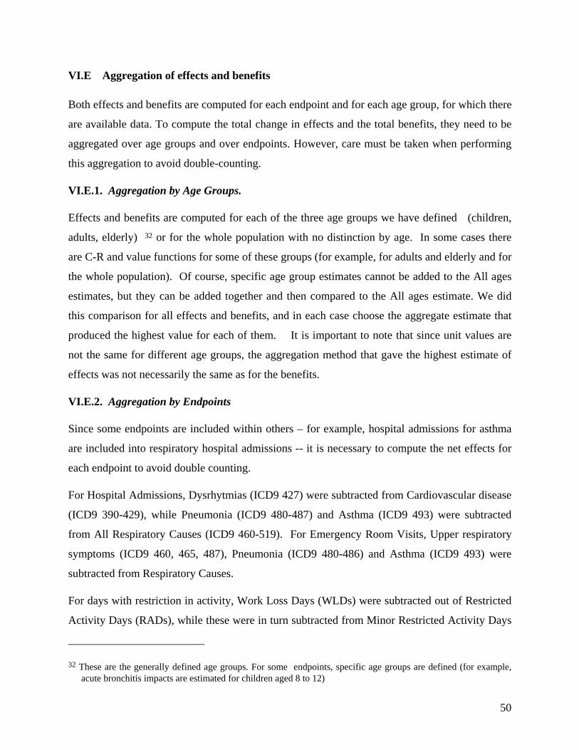
50

VI.E Aggregation of effects and benefits

Both effects and benefits are computed for each endpoint and for each age group, for which there

are available data. To compute the total change in effects and the total benefits, they need to be

aggregated over age groups and over endpoints. However, care must be taken when performing

this aggregation to avoid double-counting.

VI.E.1. Aggregation by Age Groups.

Effects and benefits are computed for each of the three age groups we have defined (children,

adults, elderly) 32 or for the whole population with no distinction by age. In some cases there

are C-R and value functions for some of these groups (for example, for adults and elderly and for

the whole population). Of course, specific age group estimates cannot be added to the All ages

estimates, but they can be added together and then compared to the All ages estimate. We did

this comparison for all effects and benefits, and in each case choose the aggregate estimate that

produced the highest value for each of them. It is important to note that since unit values are

not the same for different age groups, the aggregation method that gave the highest estimate of

effects was not necessarily the same as for the benefits.

VI.E.2. Aggregation by Endpoints

Since some endpoints are included within others – for example, hospital admissions for asthma

are included into respiratory hospital admissions -- it is necessary to compute the net effects for

each endpoint to avoid double counting.

For Hospital Admissions, Dysrhytmias (ICD9 427) were subtracted from Cardiovascular disease

(ICD9 390-429), while Pneumonia (ICD9 480-487) and Asthma (ICD9 493) were subtracted

from All Respiratory Causes (ICD9 460-519). For Emergency Room Visits, Upper respiratory

symptoms (ICD9 460, 465, 487), Pneumonia (ICD9 480-486) and Asthma (ICD9 493) were

subtracted from Respiratory Causes.

For days with restriction in activity, Work Loss Days (WLDs) were subtracted out of Restricted

Activity Days (RADs), while these were in turn subtracted from Minor Restricted Activity Days

32 These are the generally defined age groups. For some endpoints, specific age groups are defined (for example, acute bronchitis impacts are estimated for children aged 8 to 12)

51

(MRADs), to avoid double counting. Due to the differences in studies and in the quality of the

health information, it might happen that a specific endpoint yields a bigger estimate than a more

general one that includes it. In that case, the more general endpoint estimate was set to zero, not

to a negative number.

VI.E.1.1 Mortality impacts aggregation:

Mortality is one of the main sources of benefits. We could estimate both the time-series (short-

term) exposure effects (based on local Latin-American studies), and the cohort-based (long-term)

exposure effects (based on US studies). The E1 scenario includes only short-term exposure

mortality because only that type of study is available in LA. The E2 scenario includes long-term

exposure mortality, as in most studies of this type assume that long-term mortality models

already capture the short-term effects (and indeed, the mortality coefficient for the long-term

effects is three times that for the short-term effects). This difference is likely to be the single

most important difference in our scenarios.

For the E1 scenario, we compared the estimates from the All age group with the sum of the

Children and Elder estimates, using the higher estimate in each city. For the E2 scenario all the

premature deaths were computed for the population older than 30 years (following the

population canvassed in the Pope et al study), but we used the higher death estimate comparing

the All Causes estimates with the sum of the Cardio-pulmonary and Lung Cancer estimates.

Additionally, we also consider a linear and log –linear specification for the long-term mortality

function (under E2) .

Values for foregone output (lost productivity) and medical treatment costs are summed, and

labeled Cost of Illness (COI) values. The willingness to pay estimates for each Latin American

city are presented separately.

52

VII. Results

Below, we present results for each stage of our damage function analysis and for the various

scenarios. First, we present the air quality improvements associated with our scenarios. Then, we

present the reduction in the number of cases for each of the endpoints analyzed. Later, we

present the monetized benefits associated with the reduction in cases. Then, we present an

analysis that decomposes the results to explain the causes of differences in benefits across cities.

Finally, we compare our results to some published analyses of the benefits of air pollution

reductions.

VII.A Air Quality Improvements

Figure VII-1 provides baseline concentrations and post-control scenario concentrations for each

city by scenario. The full length of the bar is the baseline, the reduction in concentrations in C1

is registered by the first area to the left of the furthest extent of the bar and the further reduction

in concentrations (if any) from the C2 scenario is registered by the next area of the bar. The

remaining area of the bar is the concentrations left after application of the C2 scenario (or C1

scenario where there is no change for C2). A significant fraction of the 41 cities exceed the

annual standard (50 ug/m3), with the highest concentrations registered in Tegucigalpa,

Honduras, exceeding the standard by over 4 times. Of this group, thirteen cities have PM10

concentrations below the standard, so the reduction required in C2 is null.

53

Figure VII-1 Baseline and two control scenarios for PM10 concentrations reductions, by city (µg/m3 annual average).

0 20 40 60 80 100 120 140 160

Cities with Monthly Data -----Campinas, BR

Canoas, BRCubatao, BR

Porto Alegre, BRSao Paulo, BR

Sao Jose Do Campos, BRSorocaba, BR

Vitoria, BRCalama, CL

Santiago, CLTemuco, CLBogota, CO

Cali, COGuadalajara, MX

Juarez, MXMexico City, MX

Monterrey, MXValle De Toluca, MX

Panama City, PAKingston, JA

Cities with Annual Data ------Buenos Aires, AR

Cordoba, ARMendoza, AR

Caxias, BRCuritiba, BRItaguai, BR

Rio De Janeiro, BRSao Joao De Meriti, BR

Heredia, CRSan Jose, CRGuayaquil, EC

Quito, ECSan Salvador, ESTegucigalpa, HO

Managua, NILima, PE

Montevideo, URCaracas, VZ

ug/m3

Reduction in C2 (less C1)

Reduction in C1

However important the concentrations are, the most important metric is the population exposure,

i.e. the number of people exposed to a certain concentration. We have computed the total

exposure for all cities, by age group, as shown in Figure VII-2. This figure shows that, of the

almost 100 million people of the cities considered, a stunning 84 million are exposed to

concentrations at or above the reference value of 50 µg/m3 , of which almost 28 million are

children. Even when only A cities are considered, for which data quality is less of a concern, the

figure is still high, up to 44 million.

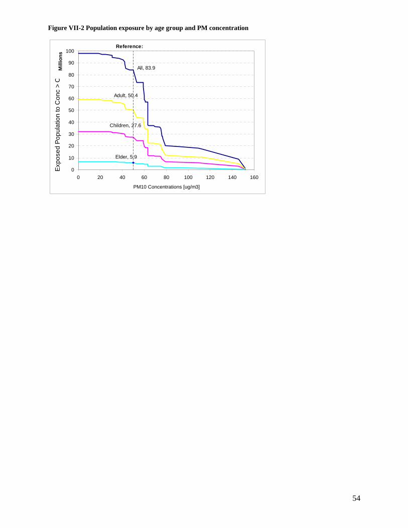
54

Figure VII-2 Population exposure by age group and PM concentration

All, 83.9

Children, 27.6

Adult, 50.4

Elder, 5.9

0

10

20

30

40

50

60

70

80

90

100

0 20 40 60 80 100 120 140 160

Mill

ions

PM10 Concentrations [ug/m3]

Expo

sed

Popu

latio

n to

Con

c >

C

Reference:

55

VII.B Health effects reductions

VII.B.1 Mortality effects

Premature mortality cases were computed applying the corresponding C-R functions and PM10

concentrations to the baseline cases. Table VII-1 provides estimated mortality effects for the

year 2000 for control scenarios C1 and C2, for the two health scenarios E1 and E2 (recall the E1

scenario is based on a linear C-R function, while the E2 uses a log-linear specification.) .

The difference in magnitude between the E1 and E2 scenarios stems from two facts: the different

specification of the concentration-response functions, and the different causes of death

considered in each scenario. For E2 the relative size of the death reductions is more important

than its magnitude. On average E2 deaths reduced are 23% higher than for E1, but for the A

cities, which have lower baseline concentrations, E2 death are reduced 39% more than E1

deaths, while for the B cities, which have higher baseline concentrations, E2 deaths are reduced

only 7% more.33

The differences between estimates of deaths averted across the two control scenarios ranges from

about 50% ( 270 vs. 130 for Lima) to 600% (9 vs. 52 for Mendoza) for the C1 case, and from

80% ( 1700 vs. 1300, again for Lima) to 260% for the C2 scenario (62 vs. 160 for Panama City).

These differences are due to what may be termed model uncertainty, i.e. the model chosen to

represent the impacts of air pollution. There also is statistical uncertainty, which arises from the

fact that the coefficients on the C-R functions are estimated. Both statistical and model

uncertainty are discussed later.

Of all the cities, Buenos Aires and Mexico City, by virtue of their large population, bad air

pollution and high mortality coefficients, are far and away the greatest beneficiary of a policy to

reduce PM10 , whether by 10% or to the annual standard. For Buenos Aires, the premature death

33 Note the different causes of death considered in the E1 and E2 scenarios. For the E1 case, we use all cause mortality, while for the E2 case, we estimate the deaths reduced as cardiopulmonary plus lung cancer deaths. As we said before, there might be other causes of death that are affected by air pollution that are not considered within these two groups. Also, the incidence rate data for these causes is more prone to error than the total mortality data, and it might be underestimated. The protocol to assign causes of death may differ from country to country, and with respect to the protocol used in the USA, where the original study was conducted. Lung cancer deaths are more difficult to misclassify than cardiopulmonary deaths, but the bulk of the effects are for the latter causes.

56

reductions are over five times with a C2 policy versus a C1 policy, while for Mexico they are

almost double. In all cases, these death reductions represent a large fraction (from 20 to 30% for

Buenos Aires and 10 to 25% for Mexico City) of the total deaths avoided.

Type A cities amount to about half of the cases for scenario C1, but only for 22-26% for the C2

scenario, where type B cities, due to their higher concentrations, have the biggest share of cases.

In that scenario, four cities not associated with high pollution problems, like Buenos Aires, Rio

de Janeiro, Lima and Montevideo, each amount to more than 10% of the premature deaths

reductions.

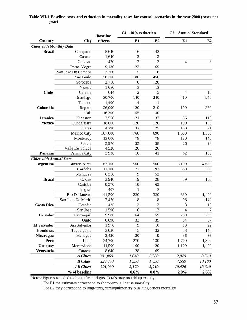
57

Table VII-1 Baseline cases and reduction in mortality cases for control scenarios in the year 2000 (cases per year)

Country City E1 E2 E1 E2

Brazil Campinas 5,640 16 42Canoas 1,640 3 12

Cubatao 470 2 3 4 8Porto Alegre 9,130 23 69

Sao Jose Do Campos 2,260 5 16Sao Paulo 58,300 180 450Sorocaba 2,710 6 20

Vitoria 1,650 3 12Chile Calama 644 2 5 4 10

Santiago 30,700 140 240 460 940Temuco 1,400 4 11

Colombia Bogota 26,000 120 210 190 330Cali 16,300 55 130

Jamaica Kingston 3,550 21 37 56 110Mexico Guadalajara 18,600 120 120 190 190

Juarez 4,290 32 25 100 91Mexico City 107,000 760 690 1,600 1,500

Monterrey 13,000 79 79 130 140Puebla 5,970 35 38 26 28

Valle De Toluca 4,520 20 26Panama Panama City 3,930 18 41 62 160

Argentina Buenos Aires 67,100 560 560 3,100 4,600Cordoba 11,100 77 93 360 580

Mendoza 6,310 9 52Brazil Caxias 3,940 19 28 59 100

Curitiba 8,570 18 63Itaguai 407 1 3

Rio De Janeiro 41,500 220 320 830 1,400Sao Joao De Meriti 2,420 18 18 98 140

Costa Rica Heredia 425 3 3 8 13San Jose 1,590 6 13 4 7

Ecuador Guayaquil 9,980 64 59 230 260Quito 6,690 33 39 54 67

El Salvador San Salvador 1,970 9 10 19 22Honduras Tegucigalpa 3,020 15 32 53 140Nicaragua Managua 3,420 20 19 36 36

Peru Lima 24,700 270 130 1,700 1,300Uruguay Montevideo 14,500 160 120 1,100 1,400

Venezuela Caracas 8,640 28 69A Cities 301,000 1,640 2,280 2,820 3,510B Cities 220,000 1,530 1,630 7,650 10,100

All Cities 521,000 3,170 3,910 10,470 13,610% of baseline 0.6% 0.8% 2.0% 2.6%

Notes: Figures rounded to 2 significant digits. Totals may no add up exactlyFor E1 the estimates correspond to short-term, all cause mortalityFor E2 they correspond to long-term, cardiopulmonary plus lung cancer mortality

Baseline Effects

Cities with Monthly Data

Cities with Annual Data

C2 - Annual StandardC1 - 10% reduction

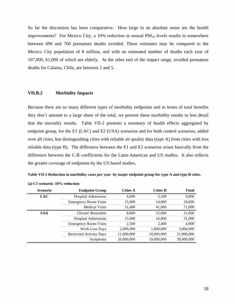
58

So far the discussion has been comparative. How large in an absolute sense are the health

improvements? For Mexico City, a 10% reduction in annual PM10 levels results in somewhere

between 690 and 760 premature deaths avoided. These estimates may be compared to the

Mexico City population of 8 million, and with an estimated number of deaths each year of

107,000, 61,000 of which are elderly. At the other end of the impact range, avoided premature

deaths for Calama, Chile, are between 2 and 5.

VII.B.2 Morbidity Impacts

Because there are so many different types of morbidity endpoints and in terms of total benefits

they don’t amount to a large share of the total, we present these morbidity results in less detail

that the mortality results. Table VII-2 presents a summary of health effects aggregated by

endpoint group, for the E1 (LAC) and E2 (USA) scenarios and for both control scenarios, added

over all cities, but distinguishing cities with reliable air quality data (type A) from cities with less

reliable data (type B). The difference between the E1 and E2 scenarios arises basically from the

difference between the C-R coefficients for the Latin-American and US studies. It also reflects

the greater coverage of endpoints by the US based studies.

Table VII-2 Reduction in morbidity cases per year by major endpoint group for type A and type B cities.

(a) C1 scenario: 10% reduction

Scenario Endpoint Group Cities A Cities B Total LAC Hospital Admissions 4,600 5,100 9,800

Emergency Room Visits 15,000 14,000 29,000 Medical Visits 31,000 41,000 71,000

USA Chronic Bronchitis 8,800 12,000 21,000 Hospital Admissions 15,000 16,000 31,000 Emergency Room Visits 2,500 2,400 4,900 Work Loss Days 2,000,000 1,800,000 3,800,000 Restricted Activity Days 11,000,000 10,000,000 21,000,000 Symptoms 20,000,000 19,000,000 39,000,000

59

(b) C2 scenario: Annual Standard

Scenario Endpoint Group Cities A Cities B Total LAC Hospital Admissions 7,400 25,000 32,000

Emergency Room Visits 16,000 66,000 83,000 Medical Visits 40,000 200,000 240,000

USA Chronic Bronchitis 13,000 48,000 61,000 Hospital Admissions 22,000 79,000 100,000 Emergency Room Visits 3,900 11,000 15,000 Work Loss Days 3,200,000 8,600,000 12,000,000 Restricted Activity Days 17,000,000 48,000,000 64,000,000 Symptoms 31,000,000 78,000,000 110,000,000

There are several results to observe about this table. First, since most of the cities have

concentrations that are higher than the annual standard (on average more than 10% higher), the

benefits from the C2 scenario are greater than in the C1 scenario. Second, reductions in hospital

admissions are about three times larger for the US scenario (E2), mainly because of the greater

coverage of different hospitalization endpoints. Also, the USA scenario includes endpoints that

are not considered at all in the LA scenario.

VII.C Benefits

In this section the monetary benefits of improving air quality in Latin American cities are

presented, first by endpoint group, then by city. Then we present the decomposition analysis by

computing benefits in dollars/person and dollars per person/ug/m3 change in PM10 .

VII.C.1 Benefits by Endpoint Group

Table VII-3 presents the aggregated benefits for all Latin American cities (distinguishing type A

and type B cities) for a 10% reduction in concentrations (Scenario C1) and reaching the 50

ug/m3 target (C2 Scenario). Benefits based on WTP and COI values are distinguished. Within

each of these value estimates Latin American C-R functions and values are used (LAC scenario)

and USA C-R functions and values are uses (USA Scenario). Figures are rounded to two

significant digits, so the totals may not match.

60

Table VII-3 Benefits By Endpoint Group (Million of US$ per year)

Benefits Scenario Endpoint Group Cities A Cities B Total Cities A Cities B Total

WTPLA Mortality 1,100 670 1,700 1,900 3,300 5,200

Hospital Admissions 0.10 0.06 0.16 0.17 0.31 0.49Emergency Room Visits 0.09 0.06 0.15 0.16 0.28 0.44

Total 1,100 670 1,700 1,900 3,300 5,200USA Mortality 21,000 24,000 45,000 33,000 110,000 150,000

Chronic Bronchitis 1,700 2,300 4,000 2,600 9,100 12,000Restricted Activity Days 430 390 820 680 1,800 2,500

Symptoms 81 77 160 120 300 430Total 23,000 27,000 50,000 37,000 120,000 160,000

Medical CostsLA Hospital Admissions 8.90 8.60 17.00 14.00 42.00 56.00

Emergency Room Visits 0.06 0.05 0.12 0.10 0.25 0.35Medical Visits 1.20 1.40 2.50 1.50 6.80 8.30

Total 10 10 20 16 49 65USA Chronic Bronchitis 170 220 400 260 880 1,100

Hospital Admissions 74 74 150 110 360 470Total 250 300 540 370 1,200 1,600

Lost ProductivityLA Mortality 63 42 100 110 210 320

Hospital Admissions 0.15 0.14 0.30 0.27 0.70 0.97Emergency Room Visits 0.02 0.01 0.03 0.02 0.06 0.08

Medical Visits 0.03 0.03 0.07 0.05 0.17 0.21Total 63 42 110 110 210 320

USA Mortality 180 150 320 300 670 970Chronic Bronchitis 660 660 1,300 1,100 2,600 3,600

Hospital Admissions 2 2 4 4 9 12Emergency Room Visits 0 0 0 0 0 0

Work Loss Days 68 43 110 120 200 320Restricted Activity Days 64 44 110 110 200 310

Total 970 890 1,900 1,600 3,600 5,200

C1 - 10% reduction C2 - Annual Standard

Note: COI estimates for mortality are based on Human Capital.

As expected, total benefits based on WTP are far larger than those based on COI. In fact, the

former are about 13-20 times larger for the C1 scenario and 14-24 for the C2 scenario. The main

component of WTP values is mortality reductions; all other endpoints contribute much less to the

benefits.

Using Latin American values rather than transferred USA values also makes a big difference --

transferred USA benefits are about 30 times greater than LAC benefits. This difference stems

from both the different number of cases considered and the unit values. The main difference

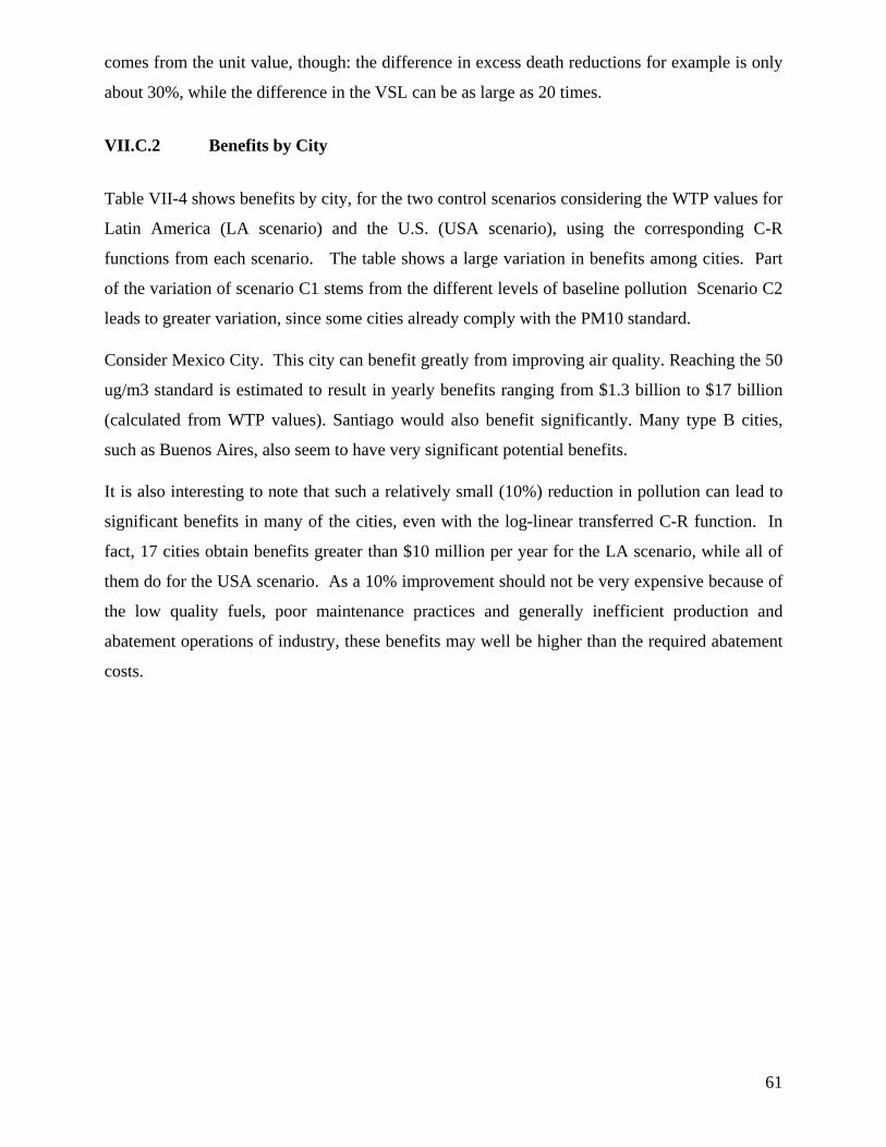
61

comes from the unit value, though: the difference in excess death reductions for example is only

about 30%, while the difference in the VSL can be as large as 20 times.

VII.C.2 Benefits by City

Table VII-4 shows benefits by city, for the two control scenarios considering the WTP values for

Latin America (LA scenario) and the U.S. (USA scenario), using the corresponding C-R

functions from each scenario. The table shows a large variation in benefits among cities. Part

of the variation of scenario C1 stems from the different levels of baseline pollution Scenario C2

leads to greater variation, since some cities already comply with the PM10 standard.

Consider Mexico City. This city can benefit greatly from improving air quality. Reaching the 50

ug/m3 standard is estimated to result in yearly benefits ranging from $1.3 billion to $17 billion

(calculated from WTP values). Santiago would also benefit significantly. Many type B cities,

such as Buenos Aires, also seem to have very significant potential benefits.

It is also interesting to note that such a relatively small (10%) reduction in pollution can lead to

significant benefits in many of the cities, even with the log-linear transferred C-R function. In

fact, 17 cities obtain benefits greater than $10 million per year for the LA scenario, while all of

them do for the USA scenario. As a 10% improvement should not be very expensive because of

the low quality fuels, poor maintenance practices and generally inefficient production and

abatement operations of industry, these benefits may well be higher than the required abatement

costs.

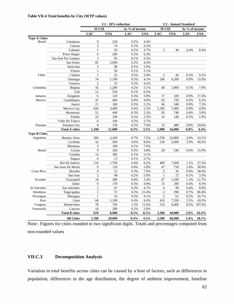
62

Table VII-4 Total benefits by City (WTP values)

LAC USA LAC USA LAC USA LAC USAType A Cities

Brazil Campinas 9 220 0.2% 4.4%Canoas 3 74 0.1% 2.5%

Cubatao 1 20 0.2% 3.7% 2 46 0.4% 8.4%Porto Alegre 8 290 0.2% 6.3%

Sao Jose Do Campos 3 83 0.1% 3.5%Sao Paulo 85 2,000 0.2% 4.4%Sorocaba 3 98 0.1% 3.9%

Vitoria 1 50 0.1% 5.1%Chile Calama 1 23 0.2% 5.0% 2 42 0.3% 9.2%

Santiago 74 1,100 0.3% 4.3% 240 4,200 0.9% 15.9%Temuco 2 53 0.2% 4.5%

Colombia Bogota 45 1,200 0.2% 5.1% 68 1,800 0.3% 7.9%Cali 12 550 0.1% 6.5%

Jamaica Kingston 6 110 0.3% 5.9% 17 320 0.9% 17.4%Mexico Guadalajara 41 460 0.4% 4.0% 62 720 0.5% 6.2%

Juarez 21 160 0.3% 2.2% 66 540 0.9% 7.5%Mexico City 650 3,400 0.4% 2.3% 1,300 7,400 0.9% 4.9%

Monterrey 51 440 0.3% 2.3% 85 740 0.4% 3.8%Puebla 22 190 0.3% 2.5% 16 140 0.2% 1.9%

Valle De Toluca 6 100 0.2% 2.7%Panama Panama City 4 130 0.2% 7.9% 13 480 0.8% 29.8%

Total A cities 1,100 11,000 0.3% 3.3% 1,900 16,000 0.8% 6.4%Type B Cities

Argentina Buenos Aires 300 3,200 0.7% 7.5% 1,700 23,000 3.9% 53.1%Cordoba 32 450 0.6% 8.6% 150 2,600 2.9% 49.2%

Mendoza 3 190 0.1% 7.0%Brazil Caxias 9 160 0.3% 4.8% 28 540 0.8% 15.9%

Curitiba 14 360 0.1% 3.1%Itaguai 0 13 0.1% 3.7%

Rio De Janeiro 110 1,700 0.4% 6.5% 400 7,000 1.5% 27.3%Sao Joao De Meriti 9 110 0.4% 5.8% 47 750 2.4% 38.0%

Costa Rica Heredia 0 12 0.3% 7.6% 2 45 0.9% 28.0%San Jose 2 49 0.2% 5.9% 1 27 0.1% 3.3%

Ecuador Guayaquil 18 280 0.4% 5.4% 67 1,100 1.3% 21.7%Quito 9 170 0.3% 4.9% 15 290 0.4% 8.3%

El Salvador San Salvador 2 47 0.2% 4.7% 4 99 0.4% 9.9%Honduras Tegucigalpa 1 72 0.2% 21.4% 2 290 0.7% 86.4%Nicaragua Managua 1 33 0.3% 9.1% 2 61 0.5% 16.7%

Peru Lima 66 1,100 0.4% 6.4% 410 7,200 2.5% 43.3%Uruguay Montevideo 78 700 1.3% 11.6% 510 6,400 8.5% 107.0%

Venezuela Caracas 16 280 0.2% 2.8%Total B cities 670 8,900 0.5% 6.5% 3,300 49,000 2.9% 43.4%

All Cities 1,700 20,000 0.4% 4.3% 5,200 66,000 1.4% 18.1%

M US$C1 - 10% reduction C2 - Annual Standard

M US$As % of income As % of income

Note:. Figures for cities rounded to two significant digits. Totals and percentages computed from

non-rounded values

VII.C.3 Decomposition Analysis

Variation in total benefits across cities can be caused by a host of factors, such as differences in

population, differences in the age distribution, the degree of ambient improvement, baseline

63

health risks, and other factors. To begin to disentangle these influences, we present benefits in

per capita terms (US$/person/year) to remove the effect of different populations, and also by unit

concentrations (US$/person/year/(µg/m3) to also remove the effect of differing magnitudes of

concentration magnitudes.

As shown in tables VII-5 and VII-6, per capita benefits for the C1 scenario have a huge range --

from as little as $0.20 to $65 per person per year for COI values. But the levels of these COI

benefits are dwarfed by those using WTP measures -- from $0.70 to $2200 per person. For the

C2 scenario the per capita benefits are even greater because the concentration reductions are

considerably larger. The differences for the LA scenario reflect differences in city characteristics,

such as concentration levels, baseline mortality, per capita income and C-R functions34.

The highest benefits per capita are for Montevideo and Buenos Aires (500 and 370

US$/person/year for the C1 scenario and 4,700 and 2,600 for the C2 scenario, respectively.

These values result from a combination of relatively wealthy (PPP=$11985 and $12081) but

very polluted (Avg PM10=158 and 117µg/m3 respectively) cities.

The average per capita benefits for all cities analyzed, for a 10% reduction in air pollution are

$17/person for the LA scenario and $500/person for the USA scenario, for WTP values. For

COI values, the average benefits are $1.30 for the LA scenario and $24 for the USA scenario.

This shows that a modest 10% reduction in particulate air pollution levels can have significant

benefits for each person of the cities analyzed.

Per capita benefits corrected for differences in changes in concentrations are shown in the last

column of tables VII-5 and VII-6). For the whole region, the population weighed average

baseline concentration is 74.7, so the 10% reduction for scenario C1 is 7.4 µg/m3. Dividing the

global unit benefits by this magnitude, we obtain the benefit per person per µg/m3, whose

average for all the cities analyzed ranges from $0.39 to $2.67 US$ per year per person per µg/m3

for the COI estimates and from $3.30 to $77.10 for the WTP values.

On a city by city basis, the COI unit benefits range from just 1 US cent per person per µg/m3 (for

Tegucigalpa and Managua, LA scenario) to $9 per person per µg/m3 (Canoas, Brazil, USA

scenario). For WTP, the unit benefits range from $0.1 (Tegucigalpa, LA scenario) to $120

(Mendoza, USA Scenario). Obviously, these differences are huge. The average for the whole

64

region for COI values are $0.20 and $3.50/person/(µg/m3) for the LA and USA scenario

respectively, while for WTP values the averages are $2.50 and $68 /person/(µg/m3) for the same

scenarios.

34 For the E2 scenarios the differences do not reflect the C-R functions, since all cities are assigned the same functions.

65

Table VII-5 Per Capita Benefits for each city (WTP values)

LAC USA LAC USA LAC USAType A Cities

Brazil Campinas 9 220 2.1 50Canoas 9 240 3.7 94

Cubatao 10 190 21 430 1.5 29Porto Alegre 6 210 1.6 55

Sao Jose Do Campos 6 180 1.7 51Sao Paulo 8 190 1.6 37Sorocaba 6 200 2.0 62

Vitoria 4 170 1.3 59Chile Calama 6 170 11 310 1.0 26

Santiago 14 210 45 780 1.8 27Temuco 9 210 1.8 44

Colombia Bogota 7 170 10 270 1.1 28Cali 3 130 0.7 29

Jamaica Kingston 10 170 26 490 1.4 23Mexico Guadalajara 11 120 17 190 1.9 20

Juarez 17 130 54 440 2.3 17Mexico City 34 180 70 380 5.4 27

Monterrey 16 130 26 230 2.6 22Puebla 17 150 13 110 3.3 27

Valle De Toluca 5 82 1.2 19Panama Panama City 5 150 16 580 0.6 20

Average A Cities 10.0 171.5 14.7 200.5 1.9 36.5 Type B Cities

Argentina Buenos Aires 35 370 190 2,600 3.0 31Cordoba 24 330 110 1,900 2.5 33

Mendoza 4 230 1.9 120Brazil Caxias 12 210 36 700 1.6 28

Curitiba 9 230 2.8 69Itaguai 4 160 1.6 70

Rio De Janeiro 18 280 68 1,200 2.3 35Sao Joao De Meriti 19 250 100 1,700 1.7 22

Costa Rica Heredia 4 120 15 450 0.6 16San Jose 6 160 4 88 1.2 29

Ecuador Guayaquil 9 140 34 570 1.2 18Quito 6 120 10 210 1.1 20

El Salvador San Salvador 4 97 9 210 0.7 15Honduras Tegucigalpa 1 85 3 340 0.1 10Nicaragua Managua 1 38 2 70 0.2 6

Peru Lima 9 140 54 960 0.6 10Uruguay Montevideo 57 500 370 4,700 3.6 31

Venezuela Caracas 9 150 2.1 35Average B Cities 12.8 200.6 55.8 872.1 1.6 33.2

Average All cities 11.3 184.9 33.7 510.5 # 1.8 35.0

C2 - Annual StandardC1 - 10% reductionUS$/person US$/person/ugm3

66

Table VII-6 Per Capita Benefits for each city (COI values)

LAC USA LAC USA LAC USAType A Cities

Brazil Campinas 0.8 19 0.19 4.6Canoas 0.8 22 0.33 9.0

Cubatao 0.9 28 2.0 59 0.15 4.4Porto Alegre 0.5 11 0.14 3.1

Sao Jose Do Campos 0.5 16 0.16 4.6Sao Paulo 0.8 11 0.16 2.2Sorocaba 0.6 14 0.18 4.7

Vitoria 0.3 9 0.12 3.1Chile Calama 0.6 17 1.0 29 0.09 2.8

Santiago 1.1 16 3.8 49 0.15 2.1Temuco 0.7 19 0.15 4.1

Colombia Bogota 0.6 18 0.8 28 0.09 3.2Cali 0.2 8 0.06 1.9

Jamaica Kingston 0.7 15 2.0 40 0.11 2.2Mexico Guadalajara 0.7 13 1.0 20 0.11 2.3

Juarez 1.2 32 4.0 97 0.17 4.4Mexico City 2.1 23 4.4 47 0.34 3.7

Monterrey 1.1 26 1.9 43 0.19 4.4Puebla 1.2 24 0.9 18 0.22 4.5

Valle De Toluca 0.4 10 0.09 2.3Panama Panama City 0.4 11 1.4 37 0.05 1.5

Average A cities 0.8 17.2 1.1 22.2 0.2 3.6 Type B Cities

Argentina Buenos Aires 2.6 48 15.0 230 0.23 4.2Cordoba 1.7 31 8.2 130 0.18 3.3

Mendoza 0.3 6 0.14 3.2Brazil Caxias 1.0 27 3.2 80 0.14 3.8

Curitiba 0.8 21 0.25 6.7Itaguai 0.3 9 0.14 4.1

Rio De Janeiro 1.5 30 5.7 100 0.19 3.8Sao Joao De Meriti 1.7 41 9.3 190 0.15 3.8

Costa Rica Heredia 0.3 10 1.1 31 0.04 1.3San Jose 0.4 12 0.3 7 0.08 2.2

Ecuador Guayaquil 0.6 17 2.3 57 0.08 2.2Quito 0.4 12 0.7 20 0.07 2.1

El Salvador San Salvador 0.3 11 0.7 21 0.05 1.7Honduras Tegucigalpa 0.1 3 0.3 9 0.01 0.4Nicaragua Managua 0.1 2 0.1 3 0.01 0.3

Peru Lima 0.7 25 4.6 120 0.05 1.8Uruguay Montevideo 4.2 58 27.0 300 0.27 3.9

Venezuela Caracas 0.6 18 0.15 4.2Average B cities 1.0 21.2 4.4 72.1 0.1 2.9

All Cities 0.9 19.0 2.6 45.3 # 0.1 3.3

US$/person US$/person/ugm3C1 - 10% reduction C2 - Annual Standard

67

VII.C.4 Summary Benefits

Finally, table VII-7 shows a summary of the total and per capita benefits for all the cases

analyzed, separated by the type of city, as well as the benefits expressed as percentage of the

total income of the cities.

Table VII-7 Summary of total benefits (a) , per capita benefits (b), and benefits as percentage of income (c), by city type

(a) Total benefits (MUS$/year)

Benefits Scenario C1 - 10% reduction C2 - Annual Standard WTP

LAC 1,100 670 1,700 1,900 3,300 5,200 USA 11,000 8,900 20,000 16,000 49,000 66,000

COI LAC 73 52 130 130 260 390 USA 1,100 1,100 2,200 1,800 4,400 6,200

(b) Per capita benefits (US$/person/year)

Benefits Scenario C1 - 10% reduction C2 - Annual Standard WTP

LAC 17 18 17 44 103 70 USA 175 245 201 374 1,531 883

COI LAC 1 1 1 3 8 5 USA 17 30 22 42 137 83

(c) Benefits as Percentage of Income (%)

Benefits Scenario C1 - 10% reduction C2 - Annual Standard WTP

LAC 0.3% 0.5% 0.4% 0.8% 2.9% 1.4% USA 3.3% 6.5% 4.3% 6.4% 43.4% 18.1%

COI LAC 0.0% 0.0% 0.0% 0.1% 0.2% 0.1% USA 0.3% 0.8% 0.5% 0.7% 3.9% 1.7%

68

VIII. CONCLUSIONS

This paper has provided a number of pieces of evidence highlighting the importance of air

pollution from the perspective of public health and economic burdens, not just environmental

quality in some more general sense. However, the size of the problem depends on some key

judgments about uncertainties in scientific knowledge and about environmental conditions. In

this concluding section of the paper we seek to summarize and put in a broader context the many

findings flowing from our analysis, including their potential implications for air quality policy.

The first point concerns simply what we know about air quality itself. This comprehensive

survey of available air quality data indicates that 26 cities, containing 85 million people (of

which 28 million are children less than 18 years of age) out of the almost 100 million population

of the cities considered in the study, are exposed to particulate concentrations above

internationally accepted levels. For many of them (18 million, 6 of them children), the excess is

notably large (more than twice the US standard). We must also note, however, that for many of

the cities we have considered, particulate data are of very uncertain quality. For almost all cities,

moreover, data on ground level ozone or its precursors is very elusive. Based on the general

principle that good policy flows from good data as well as sound analysis, improvement in air

quality monitoring in Latin America should be a higher priority than it evidently is at the present

time.

The physical effects on health of these excess pollution levels also are quite significant. If we

look only at cities with PM concentrations above the standard, reducing concentrations to the

level of the standard would avoid on the order of 10,500 to 13,500 premature deaths as well as

well a host of illness incidents, reduced activity days, and lost productivity. The premature

deaths avoided from this air quality improvement would occur across the age distribution but

would be especially important for more sensitive elder and child populations (by some of our

estimates, 10,000 and 2,500 excess deaths avoided in these groups, respectively). The total

premature deaths avoided would be on the order of 2 to 2.6% of total deaths per annum in the

cities considered.

Benefits occur not just from reducing PM concentrations to meet the US standard but also

through further improvements below the standard, since the standard does not reflect a physical

threshold. Our other simulation of air quality improvement involved a 10% reduction in

69

concentrations in all cities. This also led to large reductions in morbidity impacts and premature

mortality, with benefits spread out over the range of cities. Indeed, for this scenario the deaths

avoided in cities meeting the standard are 12 to 25% of total deaths avoided, suggesting that just

meeting the standard should not automatically be seen as an adequate goal

These relatively significant benefits are predicted whether one relies on epidemiological studies

from Latin America or on extrapolated application of US-based studies – the latter actually

predict even larger health improvements, on the order of 30% more. The disparities across

studies and gaps in knowledge do indicate a benefit of improved public health analysis for Latin

America. But from the perspective of economic benefits analysis for air quality, this link may be

less in need of improvement than the air quality data themselves, or the economic valuations of

avoided impacts.

The benefits we estimated contain considerable uncertainty that stems from the concentration

levels in the cities, from the epidemiological studies used to compute the physical impacts, and

from the unit values used to finally value the impacts. There is no direct way to quantify the

uncertainty from the concentration levels in the cities analyzed. We have presented the results

for the cities separated by our assessment of the quality of the concentration data. To reduce this

uncertainty, monitoring networks need to be improved, both in terms of number of monitors as

well as the time resolution of the measurements and reporting of this information. Right now,

many agencies report only annual averages, without explication of the finer temporal detail

actually produced by the monitors.

Assuming the ambient concentrations of the cities are relatively well estimated, we estimated the

benefits of different reductions using two different sources, Latin America (LAC) and the USA,

for both epidemiological and valuation studies. These two sources produce benefits estimates

that differ by a factor of approximately 12 for WTP estimates, and 17 for COI estimates. This

huge difference stems mainly from the difference in unit values. For example, for mortality

benefits (which are the biggest contributor to benefits, and also the easier to compare) mortality

risk reduction benefits from the USA data are about 11 times the ones based on LAC data, while

the number of cases are only 30% more. For morbidity benefits, a direct comparison is difficult

due to the different endpoint and age group coverage of LAC and USA studies, but this very

difference in coverage is responsible for most of the difference between the two scenarios.

These results suggest that more research in LAC is needed in both the estimation of impacts and

on the valuation of them. For health impacts, the main emphasis would need to be on morbidity

70

endpoints, for which there are still few data. For valuation, the most important component is the

willingness to pay to reduce risks of death.

Although isolated research is probably being conducted at this moment, we are aware of two

more broad projects that are being carried out. One is a multi-country study sponsored by the

Health Effects Institute, which aims to assess the short-term mortality impacts applying a

uniform method in several LAC cities. This would provide consistent estimates which may

improve the estimation of premature deaths in the region. The second initiative is to apply the

contingent valuation survey of Krupnick, Cropper, Alberini and Simon (Krupnick, Alberini et al.

2002) in countries around the world, such as China, Japan, some European countries, the U.S.

and Canada. While an early version of this survey has been applied in Santiago, no further work

with this survey is on-going in LAC. However, the Colombian government is considering

mounting this survey.

In turning to the valuations, we note that our findings are sensitive to the measure used for

valuing health improvements. Economic analysis makes a solid case for use of the broader and

more inclusive “willingness to pay” measure relative to the cost-of-illness measure – the more

intangible elements included in the former, related for example to discomfort and benefit from

mortality risk reduction, are as much a part of social welfare as medical and productivity costs.

But they will not register in the national accounts, for example, and with scarce resources there

may be some pressure in the policy process to scale investments in air pollution control to the

more modest level implied by cost of illness assessments of benefits.

Even this more limited measure is nontrivial if we use the more inclusive US COI figures, which

while transferred from outside Latin America reflect more impacts than comparable Latin

American figures. According to our analysis, about $2.2B or $6.2B per annum in COI benefits

might be realized, depending on the pollution control scenario. Such figures could justify

significant investments in pollution control as a form of public health protection.

If one does accept WTP for the benefits measure, then uncertainties regarding unit valuations

need to be addressed. If we use results based only on Latin American health and valuation

assessments, we get values of $1.7 or $5.2 B depending on pollution control scenario. These

represent roughly 0.4-1.4% of income averaged over all the cities, a nontrivial valuation by any

measure. This is a large enough figure to potentially justify significant pollutant control

measures.

71

While the transfer of US WTP values for mortality risk reduction also is subject to much

uncertainty, including uncertainty about the US mortality risk reduction benefits themselves, we

have confidence in the procedure we have used, which implies a WTP value that is a larger share

of income than in the US. If we combine the transferred US unit values with health impacts also

predicted by US studies, the benefits results are roughly 12 times larger than what we get using

only Latin American based information. These larger numbers provide yet more basis for policy

intervention to improve air quality – again, on economic and public health grounds.

Notwithstanding the range of estimates we present and the largely unquantifiable uncertainties

excluded from this range, the results provide a call to action for controlling urban air pollution in

Latin American cities. What forms this action should take is not the subject of this paper.

However, in Santiago Chile, where cost benefit assessment has been used to screen air quality

improvement options, benefits information of the type we have generated has been used with

cost information to lay out a menu of potential interventions. These include new emission

standards for fixed and mobile sources (new buses, trucks, and automobiles), the retrofit of

existing diesel vehicles with particle traps, the introduction of very-low sulfur diesel fuel, street

cleaning programs, and the introduction of an emissions cap and trade system to improve

efficacy and cost-effectiveness of emissions limitations for fixed sources. The results of the

CBA informed policy making, shifting the priorities toward the measures with higher

benefit/cost ratios (CONAMA R.M. 2001). However, these benefits were not the only input that

policy makers considered. Otherwise, policies for which the B/C ratio was less than one (like

street cleaning) would not have been implemented.

In studies of US benefits and costs of air quality improvement, total benefits generally dwarf

total costs of action – though the same is not true in all cases of incremental costs and benefits

(EPA 1997; EPA 1999). In Latin America the benefits values, while larger relative to income,

still are not so large as to justify a priori any conceivable intervention. The cost-effectiveness of

different interventions is sector and country-specific. Generally, simple PM filtration measures

at stationary sources can be cost effective, as can be some targeted measures to reduce emissions

from older diesel vehicles or to introduce low sulfur diesel fuel. How far these and other

interventions can be taken while still yielding net benefits – and widely shared benefits –

requires more detailed analysis of mitigation costs. What our analysis may offer from a policy

perspective, among other points, is a stronger rationale for investigating policy options and then

robustly implementing those policies that can be justified.

72

IX. REFERENCES

Abbey, D. E., N. Nishino, et al. (1999). "Long term inhalable particles and other air pollutants related to mortality in non-smokers." American Journal of Respiratory and Critical Care Medicine 159: 373-382.

Alberini, A., M. Cropper, et al. (1997). "Valuing health effects of air pollution in developing countries: The case of Taiwan." Journal of Environmental Economics and Management 34: 107-126.

Alberini, A., A. Krupnick, et al. (2003). "“Age, Health and the Willingness to Pay for Mortality Risk Reductions: A Contingent Valuation Study of Ontario Residents”." Journal of Risk and Uncertainty 24(2002): 161-186.

Arrow, K., R. Solow, et al. (1993). Report of the NOAA Panel on Contingent Valuation. Washington, Resources for the Future.

Atkinson, R. W., H. R. Anderson, et al. (2001). "Acute effects of particulate air pollution on respiratory admissions: results from APHEA 2 project. Air Pollution and Health: a European Approach." Am J Respir Crit Care Med 164(10 Pt 1): 1860-6.

Bell, M. L. and D. L. Davis (2001). "Reassessment of the lethal London fog of 1952: novel indicators of acute and chronic consequences of acute exposure to air pollution." Environ Health Perspect 109 Suppl 3: 389-94.

Bogo, H., M. Otero, et al. (2003). "Study of atmospheric particulate matter in Buenos Aires city." Atmospheric Environment 37: 1135–1147.

Bowland, B. J. and J. Beghin (2001). "Robust estimates of value of a statistical life for developing economies." Journal of Policy Modeling 23: 385-396.

Buzby, J. C., T. Roberts, et al. (1996). Bacterial Foodborne Disease: Medical Costs and Productivity Losses. USDA, Economic Research Services, AER. 741.

Carson, R., W. M. Hanemann, et al. (1996). Was the NOAA Panel Correct About Contingent Valuation? Washington, DC: 1-28.

Carson, R. T., N. E. Flores, et al. (2001). "Contingent Valuation: Controversies and Evidence." Environmental & Resource Economics 19(2): 173-210.

Cifuentes, L., J. J. Prieto, et al. (2000). Valuation of mortality risk reductions at present and at an advanced age: Preliminary results from a contingent valuation study. Tenth Annual Conference of the European Association of Environmental and Resource Economists, Crete, Greece.

CONAMA R.M. (2001). Análisis General del Impacto Económico y Social del Anteproyecto de Plan de Prevención y Descontaminación de la Región Metropolitana. Santiago, Chile, Comisión Nacional del Medio Ambiente, Región Metropolitana: 40.

Conte-Grand, M. (2002). Impacts of GHG Mitigation on Local Air Pollution in the Buenos Aires Metropolitan Area: Valuation of Human Health Effects. Buenos Aires, Universidad del CEMA.

Cummings, R. G., D. S. Brookshire, et al. (1986). Valuing Environmental Goods: An Assesment of the Contingent Valuation Method. Totowa, NJ, Rowman & Allanheld.

73

Champ, P. A., K. J. Boyle, et al., Eds. (2003). A Primer on Nonmarket Valuation. The Economics of Non-Market Goods and Resources, Springer.

Dockery, D. W., C. A. Pope III, et al. (1993). "An association between air pollution and mortality in Six U.S. Cities." The New England Journal of Medicine 329: 1753-1759.

ECLAC (2000). Conciencia Ciudadana y Contaminacion Atmosférica: Estado de Situación en el Area Metropolitana de Santiago de Chile, Santiago, CEPAL, LC/R. 2022.

ECLAC (2002). Statistical Yearbook for Latin American and the Caribbean, Economic Commission for Latin American and the Caribbean, Statistics and Economics Projections Division.

Economic Research Service - USDA. (2003). "Foodborne illness cost calculator." from http://www.ers.usda.gov/data/foodborneillness/.

EPA (1997). The Benefits and Costs of the Clean Air Act, 1970 to 1990, U.S. Environmental Protection Agency.

EPA (1999). The Benefits and Costs of the Clean Air Act, 1990 to 2010, U.S. Environmental Protection Agency.

European Commission (1999). Externalities of Energy. "EXTERNE" PROJECT Volume 2. METHODOLOGY. Update 1998. Ezzati, M., A. D. Lopez, et al. (2002). "Selected major risk factors and global and regional

burden of disease." Lancet 360(9343): 1347-60. Farrow, R. S., E. Wong, et al. (2001). Facilitating Regulatory Design and Stakeholder

Participation-The FERET Template with an Application to the Clean Air Act. Improving Regulations. P. S. Fischbeck and R. S. Farrow. Washington DC, Resources for the Future.

Freeman III, A. M. (2003). The measurement of environmental and resource values: Theory and methods. Washington, DC, Resources for the Future.

Hernandez-Avila, M. and e. al (1995). Valuacion economica de los beneficios de reducir la contaminacion del aire en la Ciudad de Mexico, Instituto Nacional de Salud Pública, México.

Holgate, S. T., J. M. Samet, et al., Eds. (1999). Air Pollution and Health. San Diego, Academic Press.

Holz, J. C. (2000). Estimación de costos unitarios en morbilidad y mortalidad y su aplicación para calcular los beneficios del Plan de Prevención y Descontaminación Atmosférica de la Región Metropolitana. Facultad de Ciencias Económicas y Administrativas. Santiago, Chile, Universidad de Chile: 101.

Ibarrarán, M., E. Guillomen, et al. (2002). Estimate the economic value of reducing health risks by improving air quality in Mexico City: Preliminary Results. México City.

Jones-Lee, M. W., M. Hammerton, et al. (1985). "The value of safety: results from a national sample survey." The Economic Journal March: 48-72.

Jorquera, H. (2002). "Air quality in Santiago Chile: A box model approach: II.PM2.5 and PM10 particulate matter fractions." Atmospheric Environment 36(2): 331-344.

Krupnick, A., A. Alberini, et al. (2002). "Age, Health and the Willingness to Pay for Mortality Risk Reductions: A Contingent Valuation Survey of Ontario Residents." Journal of Risk and Uncertainty 24(2): 161-186.

Krupnick, A. J. and M. L. Cropper (1992). "The effect of information on health risk valuations." Journal of Risk and Uncertainty 5: 29-48.

74

Kulcher, F. and E. Golan (1999). Assigning Values to Life: Comparing Methods for Valuing Health Risks. Washington, United States Department of Agriculture.

Lin, C. A., L. A. Amador Pereira, et al. (2003). "Association between air pollution and ischemic cardiovascular emergency room visits." Environ Res 92(1): 57-63.

Mitchell, R. C. and R. T. Carson (1989). Using surveys to value public goods: The contingent valuation method. Washington, DC, Resources for the Future.

O'Ryan, R. and L. Larraguibel (2000). Contaminación del aire en Santiago: estado actual y soluciones. Documento de Tranbajo CEA N°75. C.-U. d. Chile.

PAHO (2000). ???? Pope III, C. A., R. T. Burnett, et al. (2002). "Lung cancer, cardiopulmonary mortality, and long-

term exposure to fine particulate air pollution." Jama 287(9): 1132-41. Pope III, C. A., R. T. Burnett, et al. (2004). "Cardiovascular Mortality and Long-Term Exposure

to Particulate Air Pollution: Epidemiological Evidence of General Pathophysiological Pathways of Disease." Circulation 109(1): 71-77.

Pope III, C. A., M. J. Thun, et al. (1995). "Particulate air pollution as a predictor of mortality in a prospective study of U.S. adults." American Journal of Respiratory and Critical Care Medicine 151: 669-674.

Rowe, R. D. and e. al (1995). The New York Electricity Externality Study. New YOrk, Oceana Publications.

Samet, J. M., S. L. Zeger, et al. (2000). "The National Morbidity, Mortality, and Air Pollution Study. Part II: Morbidity and mortality from air pollution in the United States." Res Rep Health Eff Inst 94(Pt 2): 5-70; discussion 71-9.

Stieb, D. M., S. Judek, et al. (2002). "Meta-Analysis of Time-Series Studies of Air Pollution and Mortality: Effects of Gases and Particles and the Influence of Cause of Death, Age, and Season." J Air Waste Manag Assoc 52: 470-484.

UNEP (2002). PROGRESS IN PHASING OUT LEAD IN GASOLINE, Governing Council of the United Nations Environment Programme.

Viscusi, W. K. (1992). Fatal Tradeoffs: Public and Private Responsibilities for Risk. New York, Oxford University Press.

Viscusi, W. K. (1993). "The Value of Risks to Life and Health." Journal of Economic Literature 31: 1912-1946.

Viscusi, W. K. and J. E. Aldy (2002). "The Value of a Statistical Life: A Critical Review of Market Estimates Around the World."

Walsh, M. P. (2005). Status Report: Low Sulfur Diesel Fuel Trends Worldwide. Memo June 13, 2005.