upgrading your excel skills
TRANSCRIPT
Excel @ ExcelTexas Association of County Auditors Spring 2019
• Upgrading your Excel Skills
Presented by Kent Reeves – Bosque and Hamilton County Auditor
Detail notes to be downloaded or printed for future Reference
1
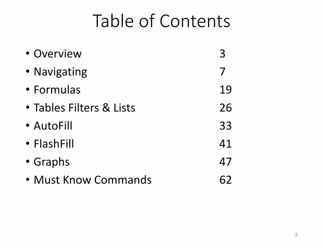
Table of Contents
• Overview 3• Navigating 7• Formulas 19• Tables Filters & Lists 26• AutoFill 33• FlashFill 41• Graphs 47• Must Know Commands 62
2
Overview
• History• Navigation• Formulas• Tables / Filters• Formatting• FlashFill / AutoFill• Graphs• Cool Tips
3

Luca Pacioli
4
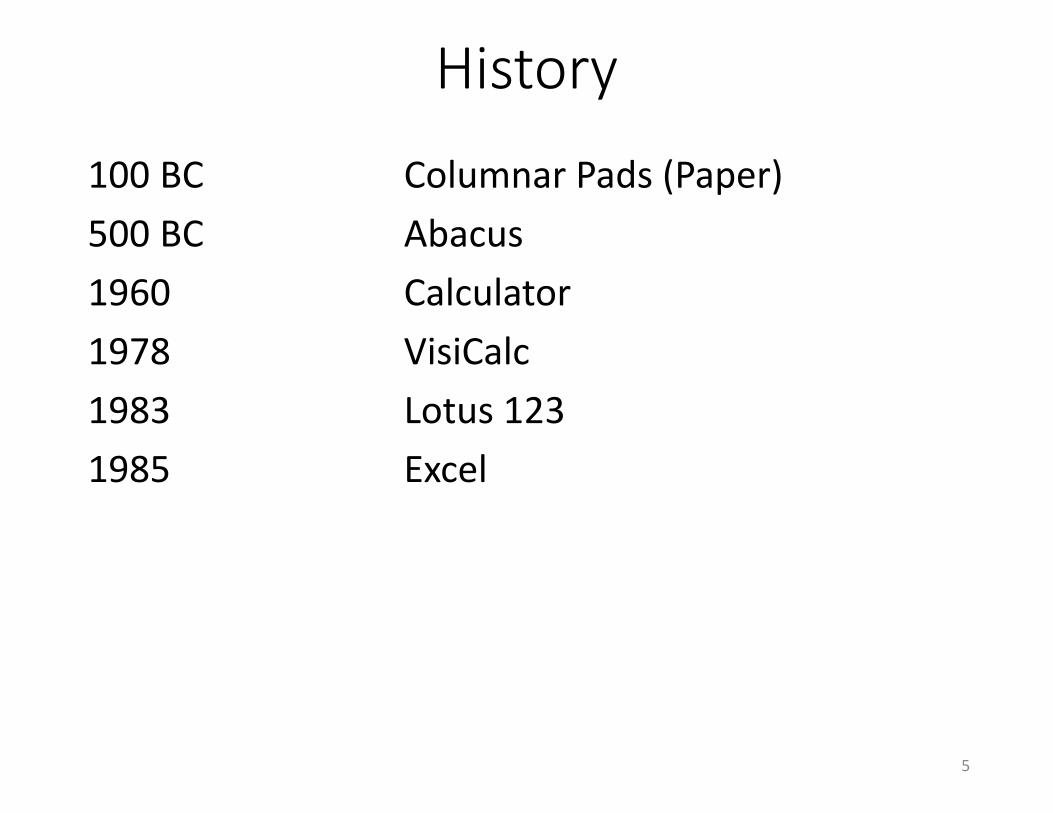
History
100 BC Columnar Pads (Paper)500 BC Abacus1960 Calculator1978 VisiCalc1983 Lotus 1231985 Excel
5
Notes
6

Navigating
• By the end of this lesson, you should be able to:
Identify the parts of the Excel windowUnderstand workbooks and worksheetsKnow how to change Excel OptionsUse shortcut keys for data entryMove around a workbook quickly and easily
7
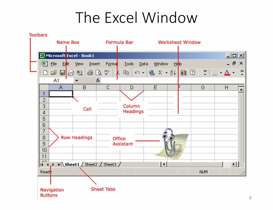
The Excel Window
8
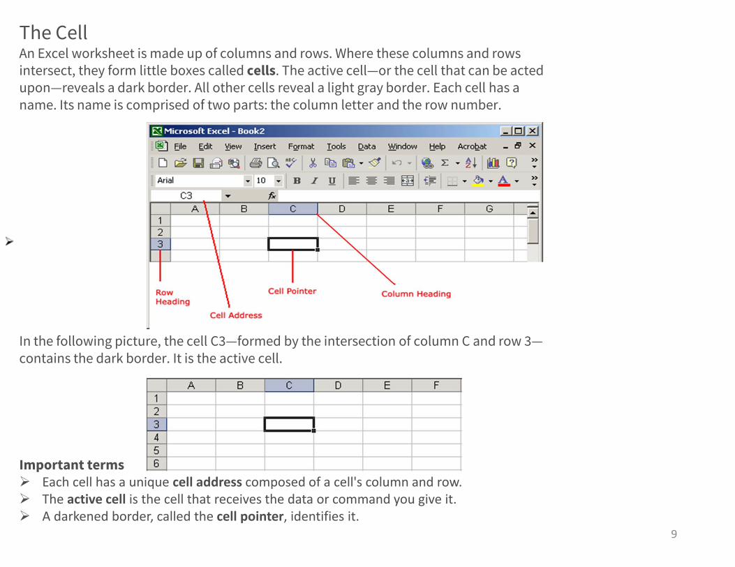
The CellAn Excel worksheet is made up of columns and rows. Where these columns and rowsintersect, they form little boxes called cells. The active cell—or the cell that can be actedupon—reveals a dark border. All other cells reveal a light gray border. Each cell has aname. Its name is comprised of two parts: the column letter and the row number.
In the following picture, the cell C3—formed by the intersection of column C and row 3—contains the dark border. It is the active cell.
Important terms Each cell has a unique cell address composed of a cell's column and row. The active cell is the cell that receives the data or command you give it. A darkened border, called the cell pointer, identifies it.
9
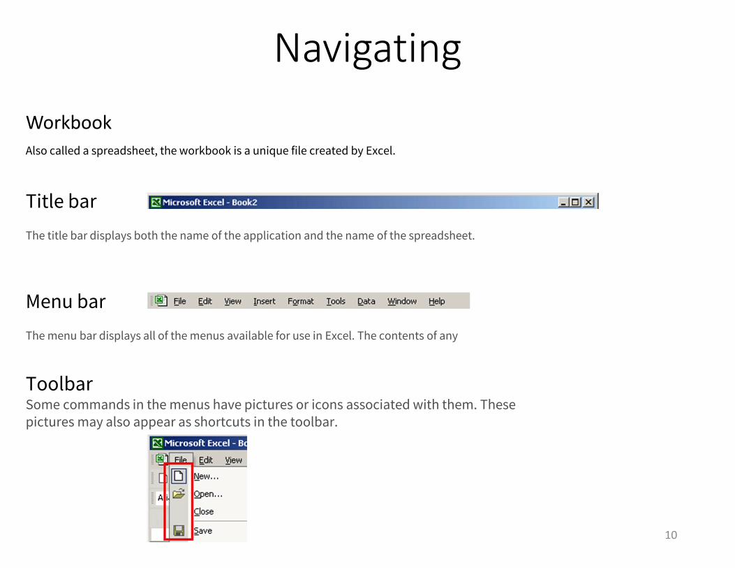
NavigatingWorkbookAlso called a spreadsheet, the workbook is a unique file created by Excel.
Title barThe title bar displays both the name of the application and the name of the spreadsheet.
Menu barThe menu bar displays all of the menus available for use in Excel. The contents of anymenu can be displayed by left-clicking the menu name.
ToolbarSome commands in the menus have pictures or icons associated with them. Thesepictures may also appear as shortcuts in the toolbar.
10

Navigating
Column headings
Each Excel spreadsheet contains 256 columns. Each column is named by a letter orcombination of letters.
Row headings
Each spreadsheet contains 65,536 rows. Each row is named by a number.
Name box
This shows the address of the current selection or active cell.
Formula bar
The formula bar displays information entered—or being entered as you type—in thecurrent or active cell. The contents of a cell can also be edited in the formula bar.
11
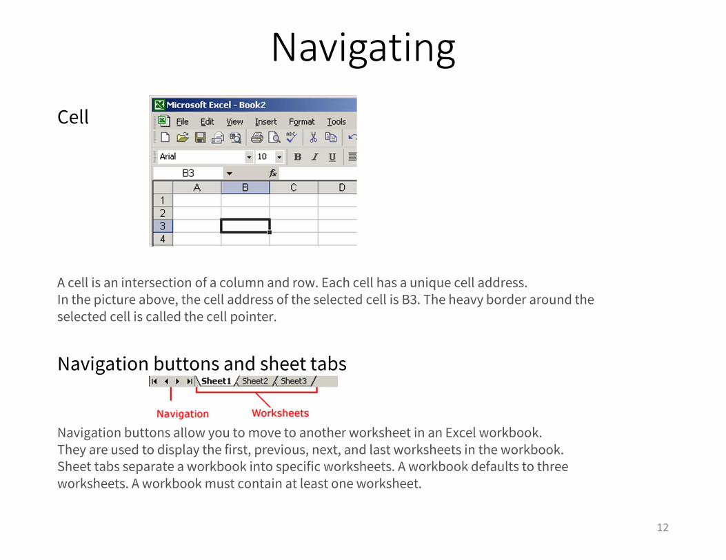
NavigatingCell
A cell is an intersection of a column and row. Each cell has a unique cell address.In the picture above, the cell address of the selected cell is B3. The heavy border around theselected cell is called the cell pointer.
Navigation buttons and sheet tabs
Navigation buttons allow you to move to another worksheet in an Excel workbook.They are used to display the first, previous, next, and last worksheets in the workbook.Sheet tabs separate a workbook into specific worksheets. A workbook defaults to threeworksheets. A workbook must contain at least one worksheet.
12

NavigatingWorkbooks and worksheets
A workbook automatically shows in the workspace when you open Microsoft Excel.Each workbook contains three worksheets.A worksheet is a grid of cells consisting of 1,048,576 rows by 256 columns.
Column headings are referenced by alphabetic characters in the gray boxes that runacross the Excel screen, beginning with column A and ending with column IV.
Rows are referenced by numbers that appear on the left and then run down the Excelscreen. The first row is named row 1, while the last row is named 65536.
Important terms
A workbook is made up of three worksheets.
The worksheets are labeled Sheet1, Sheet2, and Sheet3.
Each Excel worksheet is made up of columns and rows.
In order to access a worksheet, click the tab that says Sheet#.13

Navigation Commands
14

Customize IT
15
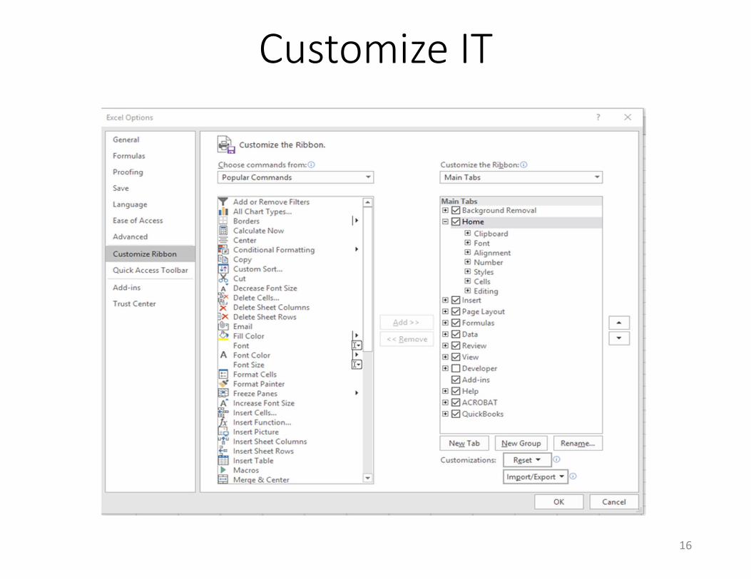
Customize IT
16
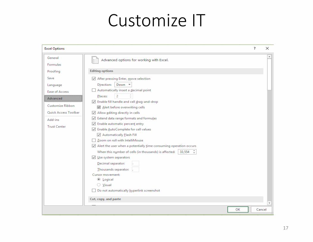
Customize IT
17

Notes
18
Formulas
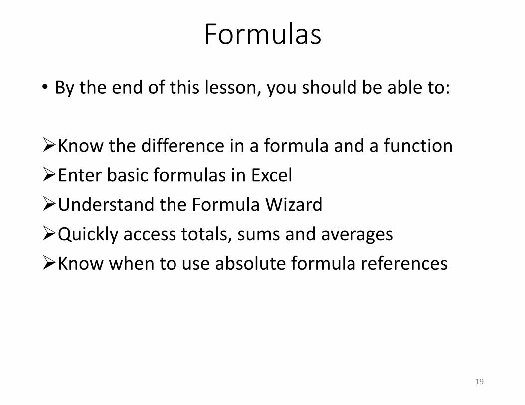
• By the end of this lesson, you should be able to:
Know the difference in a formula and a functionEnter basic formulas in ExcelUnderstand the Formula WizardQuickly access totals, sums and averagesKnow when to use absolute formula references
19

Formulas
• Formula vs Function
The difference is that a function is a built-in calculation, while a formula is a user-defined calculation. A formula could just use a single function.
For example, if you enter =AVERAGE(A1:A56) , that is a formula, using the AVERAGE function
20

Formulas
• The basics of Excel formulas• Formula is an expression that calculates the value
of a cell. For example, =A2+A2+A3+A4 is a formula that adds up the values in cells A2 to A4.
• Function is a predefined formula already available in Excel.
21

Formulas
• Formula Bar
22

Formulas
•
X 2
23
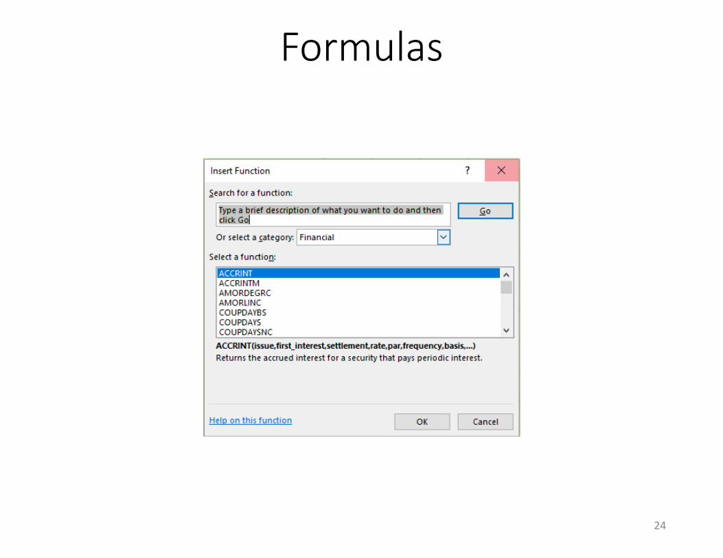
Formulas
24

Notes
25
Tables Filters & Lists
• By the end of this lesson, you should be able to:
Know how to quickly create a table in ExcelUse filters in your tableUse advanced filteringAdd summary data to your tableUse Quick Analysis Clear your formats and filters
26
Tables Filters & Lists
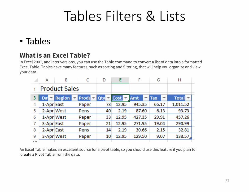
• TablesWhat is an Excel Table?In Excel 2007, and later versions, you can use the Table command to convert a list of data into a formattedExcel Table. Tables have many features, such as sorting and filtering, that will help you organize and viewyour data.
An Excel Table makes an excellent source for a pivot table, so you should use this feature if you plan tocreate a Pivot Table from the data.
27
Tables Filters & Lists
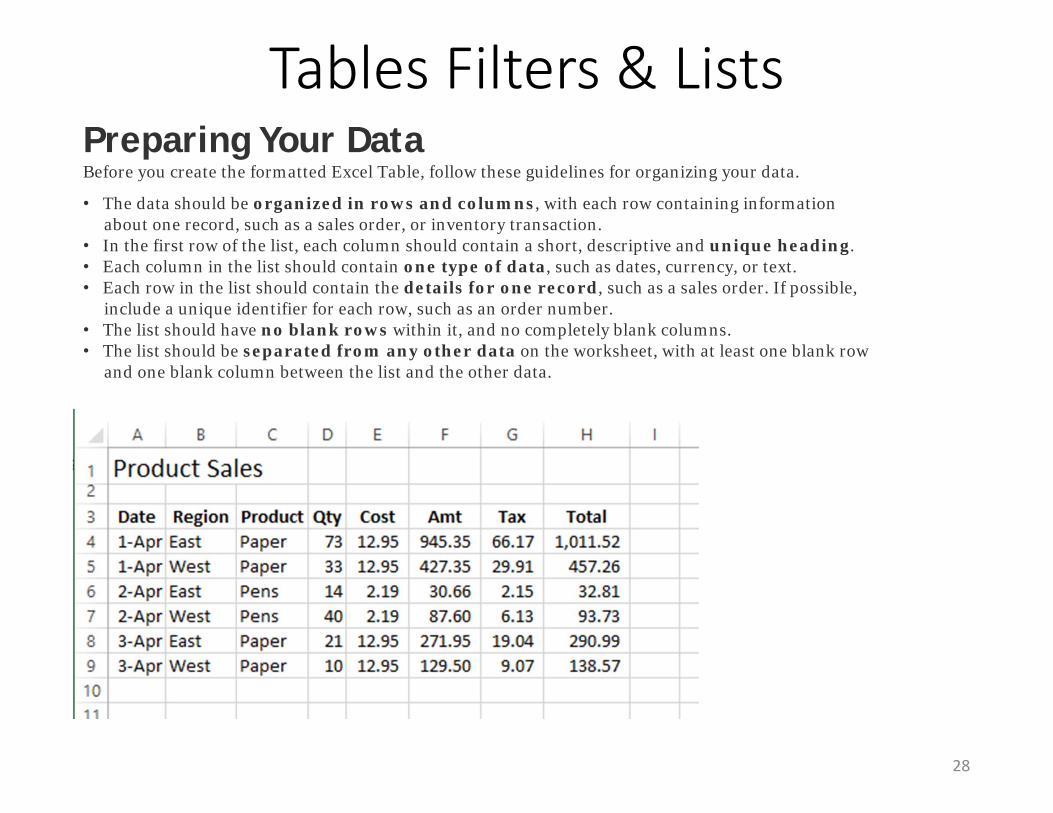
• TablesPreparing Your DataBefore you create the formatted Excel Table, follow these guidelines for organizing your data.
• The data should be organized in rows and columns, with each row containing informationabout one record, such as a sales order, or inventory transaction.
• In the first row of the list, each column should contain a short, descriptive and unique heading.• Each column in the list should contain one type of data, such as dates, currency, or text.• Each row in the list should contain the details for one record, such as a sales order. If possible,
include a unique identifier for each row, such as an order number.• The list should have no blank rows within it, and no completely blank columns.• The list should be separated from any other data on the worksheet, with at least one blank row
and one blank column between the list and the other data.
28

Tables Filters & ListsCreating an Excel TableAfter your data is organized, as described above, you're ready to create the formatted Table.
1.Select a cell in the list of data that you prepared.2.On the Ribbon, click the Insert tab.
3.In the Tables group, click the Table command.4.In the Create Table dialog box, the range for your data should automatically appear, and the My
table has headers option is checked. If necessary, you can adjust the range, and check box.5.Click OK to accept these settings.
29
Tables Filters & Lists
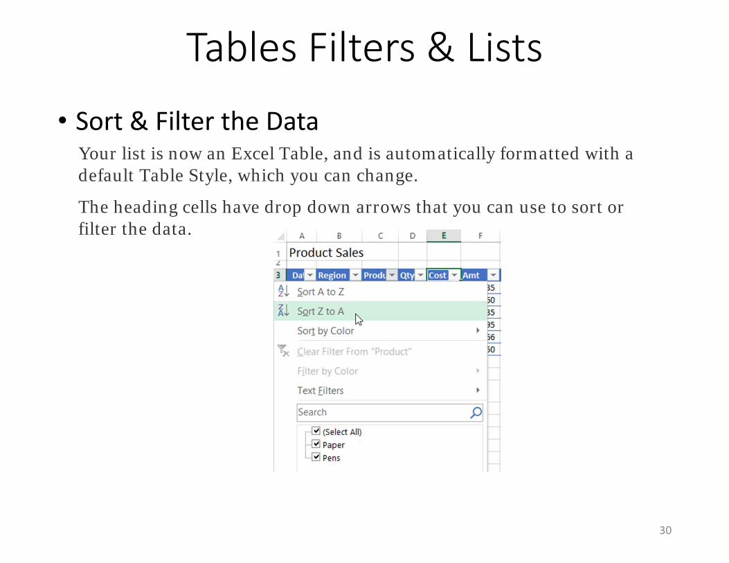
• Sort & Filter the DataYour list is now an Excel Table, and is automatically formatted with a default Table Style, which you can change.
The heading cells have drop down arrows that you can use to sort or filter the data.
30
Tables Filters & Lists
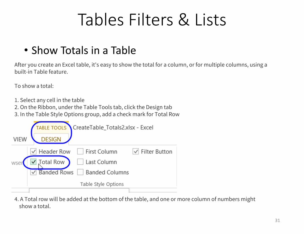
• Show Totals in a TableAfter you create an Excel table, it's easy to show the total for a column, or for multiple columns, using abuilt-in Table feature.
To show a total:
1. Select any cell in the table2. On the Ribbon, under the Table Tools tab, click the Design tab3. In the Table Style Options group, add a check mark for Total Row
4. A Total row will be added at the bottom of the table, and one or more column of numbers mightshow a total.
31

Notes
32
AutoFill
• By the end of this lesson, you should be able to:
Add Numbers/Patterns/Alphabet/Months/DatesCustomize Lists for AutoFill - AlphaQuickly Drag & Drop Data with the “Handle”
33

AutoFill
• How to Use the Fill Handle to Autofill
• The fastest way to autofill is to use Excel's Fill Handle: a plus sign that displays when the mouse hovers over the bottom right corner of a selected cell.
• Select the cell(s) containing the data you entered, drag the Fill Handle to select the cells to autofill, and release the mouse.
34
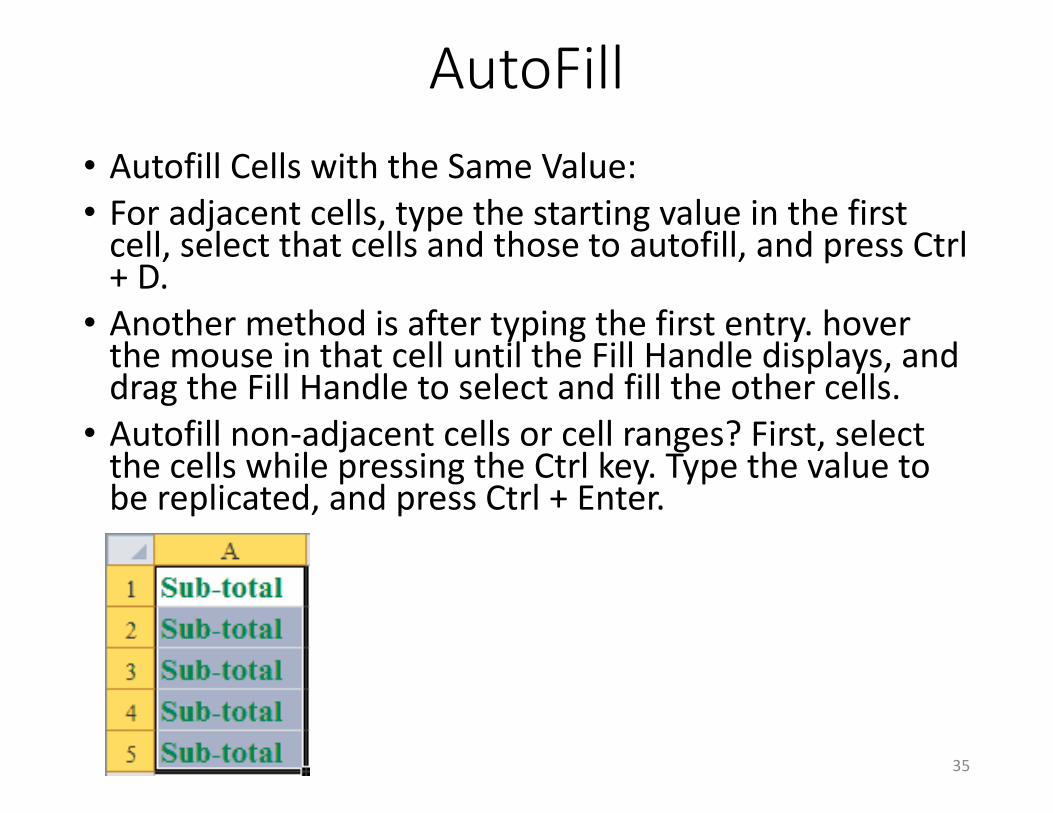
AutoFill• Autofill Cells with the Same Value:• For adjacent cells, type the starting value in the first
cell, select that cells and those to autofill, and press Ctrl + D.
• Another method is after typing the first entry. hover the mouse in that cell until the Fill Handle displays, and drag the Fill Handle to select and fill the other cells.
• Autofill non-adjacent cells or cell ranges? First, select the cells while pressing the Ctrl key. Type the value to be replicated, and press Ctrl + Enter.
35

AutoFill• Autofill Dates in Excel:• A common use of the autofill function of Excel is to autofill dates.
For sequential dates, which is the default, just type the first date and drag with the Fill Handle to select and autofill additional cells.
• The easiest way to autofill non-sequential dates is to enter the first two dates and drag with the Fill Handle to select and autofill additional cells. We cover other methods in How to Autofill Dates. Or you can enter the first date, press and hold the right-mouse button, and drag the Fill Handle to select the cells to be filled. Then click "Series" on the menu that displays, enter the desired Step Value, and click OK.
36

AutoFill• Autofill a Linear Series:• In a linear series of numbers, the same constant is added to
each number to arrive at the next number. Autofilling a linear series in Excel is easy! Enter the first two numbers, click in these cells and drag the Fill Handle up, down, left, or right to select and autofill additional cells.
• Our tutorial, How to Autofill a Linear Series, discusses other methods for autofilling a Linear Series, and how to autofill when the data cells are not contiguous, e.g. rows or columns are skipped.
37

AutoFill• Autofill a Growth Series: • In a growth series, the next number is always found by
multiplying by a constant. To autofill a growth series, enter the first two numbers, select these cells and drag the Fill Handle with the right-mouse button pressed, and click "Growth Trend" from the menu that displays.
• If you don't like using the Fill Handle, enter the first number, select it and the cells to autofill, bring up the Series Dialog Box (Fill) from the Editing section of the ribbon, click "Growth" and enter your "Step Value."
38
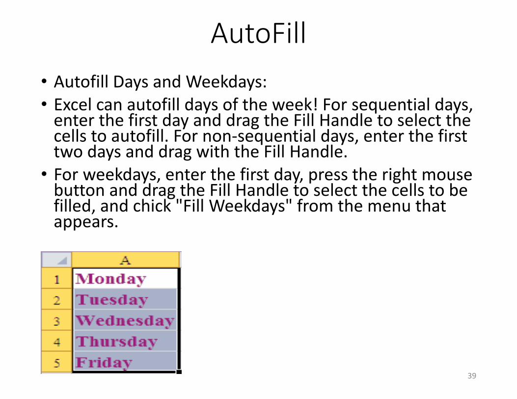
AutoFill• Autofill Days and Weekdays: • Excel can autofill days of the week! For sequential days,
enter the first day and drag the Fill Handle to select the cells to autofill. For non-sequential days, enter the first two days and drag with the Fill Handle.
• For weekdays, enter the first day, press the right mouse button and drag the Fill Handle to select the cells to be filled, and chick "Fill Weekdays" from the menu that appears.
39

Notes
40
FlashFill
• By the end of this lesson, you should be able to:
Quickly manipulate large amounts of data Change number formatsChange name formatsEnable FlashFillDisable FlashFill
41
FlashFill
• To use FlashFill:• Enter the desired information into your worksheet.
A FlashFill preview will appear below the selected cell whenever FlashFill is available, previewing FlashFill data.
• Press Enter. The FlashFill data will be added to the worksheet. The entered FlashFill data.
42
FlashFill
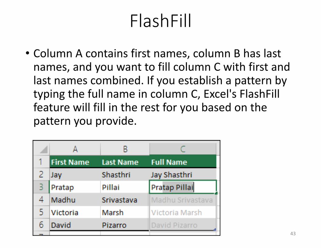
• Column A contains first names, column B has last names, and you want to fill column C with first and last names combined. If you establish a pattern by typing the full name in column C, Excel's FlashFill feature will fill in the rest for you based on the pattern you provide.
43

FlashFill
• If FlashFill doesn't generate the preview, it might not be turned on. You can go to Data > FlashFill to run it manually, or press CTRL+E. To turn FlashFill on, go to Tools > Options > Advanced > Editing Options > check the Automatically FlashFill box.
44

FlashFill
45

Notes
46

Graphs
• By the end of this lesson, you should be able to:
Quickly create a GraphUnderstand Graphs and Data relationshipsChange your Graphs to suite your needsPrint & Preview Graphs with ease
47
Graphs
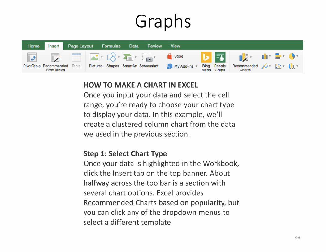
HOW TO MAKE A CHART IN EXCELOnce you input your data and select the cell range, you’re ready to choose your chart type to display your data. In this example, we’ll create a clustered column chart from the data we used in the previous section.
Step 1: Select Chart TypeOnce your data is highlighted in the Workbook, click the Insert tab on the top banner. About halfway across the toolbar is a section with several chart options. Excel provides Recommended Charts based on popularity, but you can click any of the dropdown menus to select a different template.
48

Graphs
• Step 2: Create Your Chart• From the Insert tab, click the column chart icon and
select Clustered Column.
49
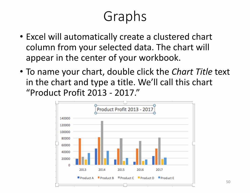
Graphs• Excel will automatically create a clustered chart
column from your selected data. The chart will appear in the center of your workbook.
• To name your chart, double click the Chart Title text in the chart and type a title. We’ll call this chart “Product Profit 2013 - 2017.”
50

Graphs
51
Graphs
52

Graphs
53

Graphs
54
Graphs
• Column Charts:• Some of the most commonly used charts, column
charts, are best used to compare information or if you have multiple categories of one variable (for example, multiple products or genres). Excel offers seven different column chart types: clustered, stacked, 100% stacked, 3-D clustered, 3-D stacked, 3-D 100% stacked, and 3-D, pictured below. Pick the visualization that will best tell your data’s story.
55

Graphs
56
Graphs
• Bar Charts:• The main difference between bar charts
and column charts are that the bars are horizontal instead of vertical. You can often use bar charts interchangeably with column charts, although some prefer column charts when working with negative values because it is easier to visualize negatives vertically, on a y-axis.
57

Graphs
58
Graphs
• Pie Charts:• Use pie charts to compare percentages of a whole
(“whole” is the total of the values in your data). Each value is represented as a piece of the pie so you can identify the proportions. There are five pie chart types: pie, pie of pie (this breaks out one piece of the pie into another pie to show its sub-category proportions), bar of pie, 3-D pie, and doughnut.
59

Graphs
60

Notes
61
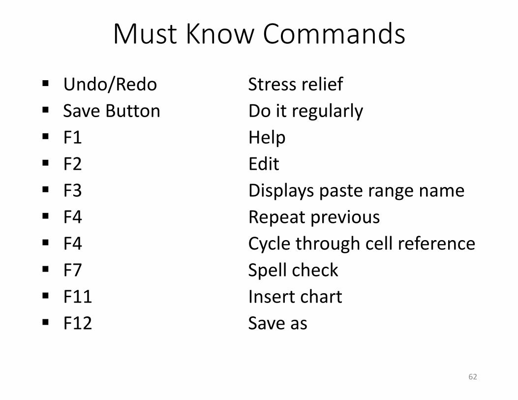
Must Know Commands Undo/Redo Stress relief Save Button Do it regularly F1 Help F2 Edit F3 Displays paste range name F4 Repeat previous F4 Cycle through cell reference F7 Spell check F11 Insert chart F12 Save as
62
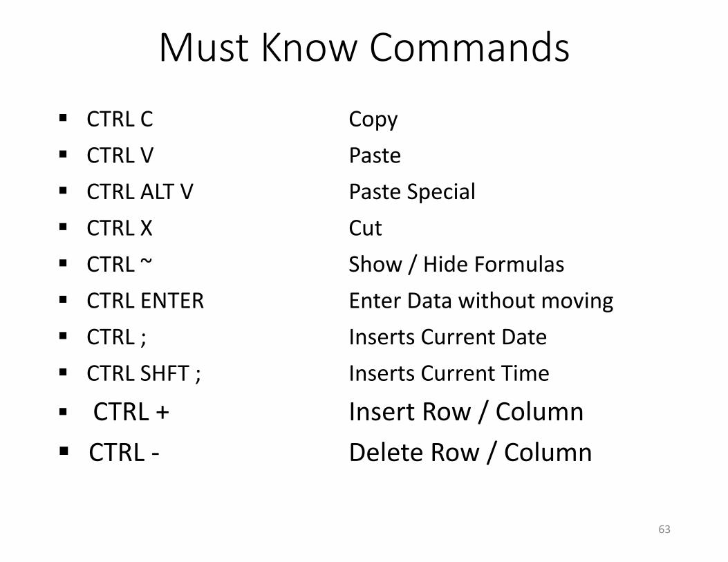
Must Know Commands CTRL C Copy CTRL V Paste CTRL ALT V Paste Special CTRL X Cut CTRL ~ Show / Hide Formulas CTRL ENTER Enter Data without moving CTRL ; Inserts Current Date CTRL SHFT ; Inserts Current Time CTRL + Insert Row / Column CTRL - Delete Row / Column
63

Must Know Commands
Password Protect Keep Data Safe SHIFT F11 Insert new worksheet
fx Formula assistant
Σ AutoSum Auto sum Clear Clear all/formats/content
64

Must Know Commands
View – Freeze Panes > Greater than < Less than >= Greater than or equal to <> Not equal to “ “ Is blank@if If this, then that
65