updated final report - penn state engineering · 2013-04-23 · updated final report american art...
TRANSCRIPT

2013
Updated Final Report
American Art Museum
Hybrid Cooling System Analysis
and
Acoustical and Structural Analysis
of New Mechanical Ductwork
Layout


April 21, 2013 [UPDATED FINAL REPORT]
Cheuk Tsang| AE | Thank you. 1
Contents Thank you....................................................................................................................................... 4
Executive Summary ...................................................................................................................... 5
Project Background ..................................................................................................................... 6
Mechanical overview .................................................................................................................. 7
MECHANICAL DEPTH --- HYBRID COOLING SYSTEM
Purposes ....................................................................................................................................... 10
Design Criteria ............................................................................................................................. 11
Programs of Utility Rates and Installation Provided ConEd Steam .................................. 12
Process of Utility Cost Predictions.......................................................................................... 14
Electric Cost prediction ...................................................................................................... 15
Prediction of Steam Utility Rate ......................................................................................... 16
Prediction of Natural Gas Utility Price ............................................................................... 18
Water Cost prediction ........................................................................................................ 20
Settings of Energy Stimulation ................................................................................................... 21
Energy Model .......................................................................................................................... 21
Assumptions Made in Analysis ............................................................................................... 21
Cooling system .................................................................................................................... 21
Prediction of utility cost ...................................................................................................... 21
Conclusion Potential inaccuracy of the stimulation .......................................................... 21
Result of the Hybrid Cooling System Analysis.......................................................................... 22
Natural Gas Hybrid System vs. Electric Cooling System ................................................. 28
Natural Gas Hybrid System vs. Steam Hybrid System ..................................................... 28
Steam Hybrid System vs. Electric Cooling System .......................................................... 29
Steam Hybrid Systems - Double Staged vs. Single Staged Absorption Chiller............ 29
Change of Cooling System Needed to Adopt the New Chiller .......................................... 30
Different Refrigerants .............................................................................................................. 31
Different Flow Rates ................................................................................................................ 32
Different Voltages ................................................................................................................... 34
Different Dimensions ............................................................................................................... 35
Analysis of Operation Sequences for Hybrid System ............................................................. 39

April 21, 2013 [UPDATED FINAL REPORT]
Cheuk Tsang| AE | Thank you. 2
Purpose ..................................................................................................................................... 39
Analysis of Operation Sequence .......................................................................................... 39
Progress of Building Energy Model and Calculating Annual Utility Cost ..................... 39
Result of Operation Sequence Analysis ............................................................................... 45
Conclusion ............................................................................................................................... 46
Economic Analysis ...................................................................................................................... 47
Current Condition of Utility Rate ........................................................................................... 47
Future Plant of ConEdison Power Generation and Other Utilities .................................... 48
Overall Conclusion ..................................................................................................................... 50
Technical Conclusion—Why Natural Gas Fired Absorption Chillers? .............................. 50
Economical Conclusion—Price of Natural Gas and Future Plan of AAM Mechanical
System ....................................................................................................................................... 51
STRUCTURAL AND ACOUSTICAL BREADTHS-- NEW MECHANICAL DUCTWORK LAYOUT
Purposes ....................................................................................................................................... 52
Design Criteria ............................................................................................................................. 52
Placement of Mechanical Equipment ................................................................................ 52
Redundancy of Ventilation Systems in AAM....................................................................... 52
Structural System of AAM ....................................................................................................... 53
Acoustical control of AAM .................................................................................................... 53
Proposed Air Handling Unit Locations and Ductwork Layout .............................................. 53
Result with 3 perspectives: Mechanical, Structural and Acoustical ................................... 55
Mechanical Perspective ........................................................................................................ 55
Structural Perspective............................................................................................................. 56
Acoustical Perspective .......................................................................................................... 57
Conclusion ................................................................................................................................... 59
Works Cited ................................................................................................................................. 61
Appendix. A Hybrid System Combination List ........................................................................ 64
Appendix. B Consumption of Hybrid System Combinations ................................................ 65
Appendix. C Utility Cost Predictions Equations of All Hybrid System Combinations ......... 67
Appendix. D Annual Utility Cost without Inflation Rates of Hybrid System Combinations 70
Appendix. E Interest Rates and Projected furl price indices Used in Sensitive Analysis .... 73

April 21, 2013 [UPDATED FINAL REPORT]
Cheuk Tsang| AE | Thank you. 3
Appendix. F Sensitive Analysis Results of All Combinations .................................................. 74
Appendix. G Sensitive Analysis Results of All Operation of Sequences .............................. 77
Appendix. H Ventilation Distribution of Supplying Air to Galleries and Offices ................. 79
Appendix. I Information of New Air Handling Units Referenced by Trane ......................... 80
Appendix. J Duct Sizing of New Ductwork layout ................................................................. 81
Appendix. K Structural System Check ..................................................................................... 86
Deck Check ............................................................................................................................. 86
Beams ....................................................................................................................................... 87
Columns ................................................................................................................................... 89
Appendix. L Noise Criteria Charts ............................................................................................ 90
MAE Course Relation ................................................................................................................. 94

April 21, 2013 [UPDATED FINAL REPORT]
Cheuk Tsang| AE | Thank you. 4
Thank you.
For …
Turner Construction Company Offering American Art Museum for my
thesis project
Mr. Benjamin Gordon Providing us building information
All the AE Professors Helping and Supporting me in these years
Corey Wilkinson and Copy Center Computer troubleshooting
Students shared the same thesis project
with me (Sean Felton, Chang Liu, and
Vincent Rossi)
Sharing news and ideas of AAM thesis
project
Class of AE 222 Building a Revit model of AAM
My family and My Studio Roommates (Andrew Voorhees, Brice Ohl, Daniel
Bodde, Jonathan Fisher, Jonathan Gallis,
Mingao Li, Sarah Bednarick, etc. )

April 21, 2013 [UPDATED FINAL REPORT]
Cheuk Tsang| AE | Executive Summary 5
Executive Summary After analyzing the mechanical system of American Art Museum (AAM), two
proposed ideas are conducted a further and detail analyses. The overall report is
focused on the cost effectiveness of mechanical system.
Mechanical Depth – Hybrid Cooling System
Today, the price of No.2 oil is increasing. And, the utility company, ConEd, which
is contracted with AAM, generates electricity by fueling oil. As other fuels, the
applications provide either attractive incentive and/or rebate programs or relatively
lower price. Therefore, a hybrid cooling system is suggested to seek for further saving
with the highly energy efficient mechanical system. After conducting an exhaust
search of the best hybrid system, it found that the best system is two natural gas-
fired single stage absorption chillers and one electric centrifugal chiller with 5 year
payback period.
Structural and Acoustical Breadths – New Ductwork layouts
AAM will consist of 3 mechanical floors. Two out of three floors will hold
ventilation systems, which will serve different floor levels. The ventilation system on
cellar level will serve conditioned air from cellar level to 7th floor, and the ventilation
system on 9th floor will deliver air to 8th floor only. So, the proposed idea is to bring
more AHU closer to the load with the consideration of minimizing the structural
impact and acoustical impact. Overall, the result shows that the proposed duct
work layout will save about $36,000 by reducing the amount of ducts.
After conducting the studies of two ideas, it shows that there are more potential
savings of AAM mechanical system. For example, the fuel type of AAM should be
more toward natural gas. And, the area of 9th floor would be increased and more
AHUs can be put on 9th floor to be closer to the load, if the aesthetics of AAM is not
affected.

April 21, 2013 [UPDATED FINAL REPORT]
Cheuk Tsang| AE | Project Background 6
Project Background
Name American Art Museum
Figure 1 Courtesy of the owner
Figure 2 Courtesy of the owner
Figure 3 Courtesy of the owner
Location New York, NY
Occupancy
Type
Group A-3 Museum
Size 195000 sq. ft.
Function Gallery, Classroom, Office,
Auditorium, Restaurant
Floors 9 levels with cellar
mezzanine and cellar level
underground
Construction Start in February 2012, End
in late 2014
Main
Architectural
Feature(s)
1. Cantilevered
entrance
2. The Biggest column-
free gallery in New
York
3. Ground floor
restaurant and top
floor café
4. Rooftops on
Multiple levels for
outdoor exhibition
5. Glazing system, pre-
cast concrete, and
stud wall as façade
Sustainability Goal: LEED Gold
Certification

April 21, 2013 [UPDATED FINAL REPORT]
Cheuk Tsang| AE | Mechanical overview 7
Mechanical overview
Heating and Cooling System
Cooling System
The main cooling system will consist of three 300 tons electrically driven
centrifugal chillers with utilizing refrigerants R-123 or R-134a. This cooling system design of
AAM takes a big advantage of free cooling. On the roof, there will be 5 cooling towers,
and each of them will hold 200 ton cross-flow or counter-flow typed cells. A plate and
frame free cooling heat exchange will be installed in this system.
The following figure is the monthly cooling load profile of AAM. The cooling load
profile is similar to a profile of a typical commercial, because the AAM will be operated
with the schedule similar to a commercial building.
Figure 4 cooling load profile of AAM
0
20
40
60
80
100
120
140
160
1 2 3 4 5 6 7 8 9 10 11 12
Ele
ctr
icity
(M
Wh
)
Month
Cooling Load
Cooling

April 21, 2013 [UPDATED FINAL REPORT]
Cheuk Tsang| AE | Mechanical overview 8
Heating System
A hot water heating boiler plant also will be located on Cellar level. This plant will
consist of 5 condensing boilers generating hot water with 150 supply water and 120
return water. The system will lower its pollution by built-in water treatment and a
combustion chamber with gas filters.
Similar to the cooling system, the heating system will also have energy saving
components. First, the waste heat will be sent to a 75kW cogeneration unit to produce
extra electricity. Second, the radiation heaters will be conducted in finned tube
convector along the exterior walls to reduce heat losses.
The heating load profile of AAM is shown as the following figure. This profile
doesn’t include the data of domestic water heating, because the domestic water load
profile is not provided.
Figure 5 heating load profile of AAM
0
2000
4000
6000
8000
10000
12000
14000
1 2 3 4 5 6 7 8 9 10 11 12
The
rms
Month
Heating Load Profile
Heating

April 21, 2013 [UPDATED FINAL REPORT]
Cheuk Tsang| AE | Mechanical overview 9
Ventilation
In American Art Museum, there will be 3 air conditioning systems as cooling
systems located on the cellar Level (-1). Each of them will handle 1/3 of the load
generated from Cellar to 7th levels. The other system is located in Level 9, which only
manages the air condition in 8th floor. Because of the moisture sensitivity of artwork in
AAM, both of the main air condition system will consist of fogged type humidifier
systems. Also, the system will consist of 95% efficient filters, which stabilize the
contaminant concentration levels. For energy saving purpose, some particular zones
will be treated with variable air volume boxes, such as galleries.
Control System
The control system of American Art Museum, Direct Digital Control (DDC), will be
programed to switch modes automatically, called “Auto” mode. DDC will also receive
the data from all sensors, gradually adjust the damper position and provide the needed
de/humidification. Moreover, the control system can be remotely controlled outside of
AAM, which greatly increases the convenience.
Building Envelope
Finally, the AAM will gain good amount of LEED point on energy efficiency by
developing a well-insulated building envelope. The building envelope is particularly
designed to block solar heat gain from the sun. First, all the windows will be installed
with motorized roller shades. Second, all the windows will be applied a layer low-e
glazing.

April 21, 2013 [UPDATED FINAL REPORT]
Cheuk Tsang| AE | Purposes 10
Proposed Cooling System --- Hybrid Cooling System
Purposes In 2000s, there are several ASHRAE articles related to hybrid system (Smith, 2002).
A hybrid system is a combination of cooling system with electricity and other fuel. The
articles introduce a new combination of different chiller type to increase the capital
cost and decrease the long term utility cost. This is the starting point of the hybrid system
analysis.
This study conducts a hybrid system analysis with 3 fuel choices.
(1) Electricity is the original fuel choice of AAM cooling system.
(2) The steam is the most attractive choices, because of three rebate and incentive
programs provided by ConEdison and the greenness of steam--- the steam is the
waste heat produced from the oil power plant of ConEdison.
(3) Figure 6 'How steam is generated' from ConEdison
Oil and natural gas fueled power
plants
&
Waste steam

April 21, 2013 [UPDATED FINAL REPORT]
Cheuk Tsang| AE | Design Criteria 11
Although the LEED point in Energy and Atmosphere is fully obtained, the application of
steam driven cooling system with the waste heat of ConEdison significantly lower the
emission rate.
(4) Natural gas. Recently, as the price of electricity increase, the cost of natural gas
decreases.
This analysis is focused on the cost effectiveness and the workability of the AAM
cooling system. The workability of the cooling system should be ensured that installing a
new type of chiller doesn’t damage the cooling system as a whole. For example, the
size of the chiller room should be fit for new chiller(s), and the supply temperature of a
new chiller should match with the supply temperature of the electric chiller.
Since this analysis is to seek for a more economical hybrid system, the change of
cooling system and mechanical room will be designed to make future saving within a
short payback period.
Design Criteria According to install a hybrid cooling system, there are two limitations:
(1) The selection of fuels. The fuel options in New York are electricity, natural gas and
steam. The steam is an interesting fuel option, because of the incentive programs
offered by ConEdison, which is the only company. Since AAM already has
contracted with ConEdison for supplying natural gas and electricity. The cost
prediction, which is used to conduct the sensitive analysis, is applied on the
historical rate provided by the website of ConEdison.
(2) By adding a new type of chiller to the cooling system, it changes the
characteristics of the cooling system, such as condenser inlet and outlet water
temperatures. But, the characteristic changes do not include in this section. The
change is concluded in the water.

April 21, 2013 [UPDATED FINAL REPORT]
Cheuk Tsang| AE | Design Criteria 12
Programs of Utility Rates and Installation Provided ConEd Steam
This section details the programs of ConEd steam. These programs convince
building owners and mechanical engineers to consider the potential application of
cooling system. Also, ConEd has a large amount of case studies and related
information in its website. Therefore, the analysis in this report is conducted with these
programs and determines if the offers are beneficial to AAM.
Incentive Program of Steam Cooling System
Comparing to the cost differences with an electric centrifugal chiller and other
steam driven cooling equipment, the capital costs of a steam turbine and a steam
driven double stage chiller are triple the cost of electric centrifugal chiller (Spanswick,
2003), and the cost of a single stage chiller is 30% more than the cost of an electric
chiller (RSMeans Engineering Department, 2013 ). The incentive program helps the
owner of a building to decrease the capital cost of steam cooling system. However, this
amount of incentive only covers about 15~20% of the capital cost and doesn’t include
any single stage steam chiller.
Table 1 Incentive program of installing a steam cooling system

April 21, 2013 [UPDATED FINAL REPORT]
Cheuk Tsang| AE | Design Criteria 13
Operation Saving: Steam Air Conditioning Summer Discount Program
The steam air conditioning summer discount program in ConEd offers a rate
reduction in 2012 to promote their steam client addition or/and replacement of steam
driven air conditioning equipment. ‘Con Edison: steam operations - steam rates:
incentive programs, it states that
Steam Air-Conditioning Summer Discount Program
“As described in SC 2 and SC 3 tariff Special Provisions D and E, when a
customer installs a new or replacement steam air conditioning system, Con
Edison will provide a $2.00 per 1,000 pounds discount for cooling steam.”
------- ConEd.
This discount program is not cost effective, because the utility rates of steam in
Service Classification No. 2 and No. 3 tariff are about $20~$50 per 1,000 lbs. steam.
Maintenance Service and Annual Incentive of a Steam Cooling System
There are difficulties of maintaining the steam cooling equipment due to the
complexity. ConEd provides 24/7 steam maintenance and services, including flange,
piping, and trap repair, and another incentive program of steam cooling system.
With high convenience and no profit making, the bill will be charged in the
following month bill. In the ConEd website of ‘Why Steam FQA’, it claims that
“Labor cost: - $93 per hour from 7:30 a.m. to 3 p.m., Monday through Friday,
excluding holidays, and $111 at all other times.” ---- ConEd
(The list of Steam Repair Service is shown on the web page of ConEd, Con
Edison: steam operations - maintenance & services.)
As the steam cooling system, ConEd also provides an incentive program
associated with the service. Based on the claim of ConEd Maintenance Cost in ‘Why
Steam FQA’, the incentive program doesn’t significantly reduce the maintenance cost
of a new steam cooling system. But, providing the service of remote monitoring steam
trap behind the steam meter, it gives the client of ConEd a fully secured and trusted
maintenance system.

April 21, 2013 [UPDATED FINAL REPORT]
Cheuk Tsang| AE | Design Criteria 14
Table 2 an annual maintenance incentive of a steam cooling system1
However, due to lack the maintenance cost of the 2 chiller types, this analysis
neglects the maintenance cost study and assumes that the maintenance cost of both
system are the same.
Process of Utility Cost Predictions
Since this study heavily focus on the cost effectiveness of cooling system and
associated with the utility cost, the prediction of utility must be accurate and closed to
the future predictions provided by ConEdison and other related organizations. The
approach of predicting is to find a regression equation with a reasonably high
coefficient of determinant of utility cost. There are about 10 combinations of hybrid
systems and 4 utility costs of each combination (electricity, natural gas, steam and
water).
In the following sections, it explains in detail of conducting each utility prediction.
The figures and the regression equations posted in this section are the calculations of
the original cooling system, which predicts the utility cost from 2015 to 2035. Every
combination has 3 common regression equation to calculation the monthly cost of
water, steam, and natural gas and individual equation of electricity in order to restore
accuracy.
1 It is only eligible for the application of steam turbine or double stage absorption chiller.

April 21, 2013 [UPDATED FINAL REPORT]
Cheuk Tsang| AE | Design Criteria 15
Electric Cost prediction
AAM will have a contract with the ConEd for electricity supply. Therefore, the
historical rates of ConEd can be used in detail utility prediction. Then, the future
electricity bill is predicted from 2012 to 2035, which is a typical lifetime of a chiller.
Since in every few years, ConEd increases the electric rates and changes the
structure of electricity cost. The prediction applies the regression with annual electricity
bills in past and find the future electricity bills. For example, in the following figure, the
total annual electricity bill first is calculated the past electricity rates from 2005 to 2012.
Second, the regression is generated and based on the past electricity bill, which the
regression equation of original cooling system is shown in Figure 7. The regression
equation is a 2nd order equation and the function of year.
Figure 7 Electricity prediction of original cooling system
Every combination obtains its own regression equation to predict the electricity
cost. All regression equations of combinations are in Appendix. C.
Although the error ranges of all the electricity bill predictions are less than 5%, the
payback must be within a reasonable time period. It is because the error increases
while the number of year is increasing.
y = 4227.5x2 - 2947.6x + 344810
0
100
200
300
400
500
600
700
0 1 2 3 4 5 6 7 8 9
co
st (
$
Tho
usa
nd
s)
year
Historical rate of Electricity
electricity rate Poly. (electricity rate)
2004 2005 2006 2007 2008 2009 2010 2011 2012 2013

April 21, 2013 [UPDATED FINAL REPORT]
Cheuk Tsang| AE | Design Criteria 16
Prediction of Steam Utility Rate
The data that ConEd provides in public is from past 4 years. Since the steam
utility rate in all these years remains same billing structure, the calculation of the steam
utility prediction is done on every basic items of the bill, such as customer charge and
steam base rate.
The equations shown in the following 2 tables are used in the prediction of all
combinations. Since the prediction is based on the rates in last 4 years, the regression of
each item behaves linearly. It provides a more accurate prediction than using overall
regression equation. Therefore, every combination has the same regression equation
set.
Table 3 Base rate of steam rate No.1
y = 1.4835x + 11.833
y = 5.0181x + 29.376
y = 3.8819x + 23.736
y = 3.7296x + 22.981
0
10
20
30
40
50
60
1 2 3 4 5
co
st (
$/1
,000lb
)
Year
Historical steam base rate of steam Rate
No.1
0 to 20 Mlb in all months 20 to 50 in all months
50 to 1000 Mlb in all months 1000~ Mlb in all months
Linear (0 to 20 Mlb in all months) Linear (20 to 50 in all months)
Linear (50 to 1000 Mlb in all months) Linear (1000~ Mlb in all months)
01/2009 10/2009 10/2010 10/2011 01/2012

April 21, 2013 [UPDATED FINAL REPORT]
Cheuk Tsang| AE | Design Criteria 17
Table 4 Customer charge of steam rate No.1
The Calculation of Steam Utility Cost
Steam:
First 0~20 Mlb (1Mlb = 1000 lb.)
Next 30 Mlb
Next 950 Mlb
More than 1000 Mlb
Customer Charge
Total: The sum of all charges = monthly steam cost
y = 118.55x + 702.16
0
200
400
600
800
1000
1200
1400
1 2 3 4 5
Co
st (
$/1
,000lb
)
Year
Customer Charge of Steam Rate No.1
base rate Linear (base rate)
01/2009 10/2009 10/2010 10/2011 01/2012

April 21, 2013 [UPDATED FINAL REPORT]
Cheuk Tsang| AE | Design Criteria 18
Prediction of Natural Gas Utility Price
The cost prediction of natural gas utility price is slightly different than the previous
predictions. It is because it is difficult to stimulate a regression equation of natural gas
utility cost. In 2012, the utility cost of natural gas behaves irregularly that the cost in 2012
is significantly lower than the previous and further years. So, the natural gas historical
rate applied in the regression only takes the data after 2012 in order to restore the
accuracy.
Figure 8 Historical rate of natural gas cost factor
As Figure 8 Historical rate of natural gas cost factor it shows that the natural gas cost of
ConEdison consists of many large range fluctuations. After applying the shortened
range of historical rates, the coefficient of determination, R2 value, doesn’t fall above
0.9. It is impossible to predict the future natural gas cost accurate. So, the other
approach is conducted.
0
10
20
30
40
50
60
70
2011 2011.5 2012 2012.5 2013 2013.5
co
st (
$/t
he
rm)
Year
Historical rate of natural gas cost factor
Natural gas cost factor

April 21, 2013 [UPDATED FINAL REPORT]
Cheuk Tsang| AE | Design Criteria 19
Figure 9 Average natural gas cost factor of 2011 and 2012
The approach is to average the cost factor of 2011 and 2012 and generate regression
equations. So that, the prediction of natural gas cost factor behaves more stable and
similar to the prediction of the ConEdison’s Citygate cost of natural gas, Figure 10.
Figure 10 Con Edison’s Citygate Cost of Gas for Firm Customers (ConEdison , 2010 )
y = 12.977x - 26065
0
10
20
30
40
50
60
2011.8 2012 2012.2 2012.4 2012.6 2012.8 2013 2013.2
co
st (
$/t
he
rm)
year
Average natural gas cost factor of 2011
and 2012
$/therms Linear ($/therms)
Con Edison’s Citygate Cost of Gas for Firm Customers

April 21, 2013 [UPDATED FINAL REPORT]
Cheuk Tsang| AE | Design Criteria 20
Water Cost prediction
According to the New York City Water Board, it provides the historical rate of
water at least 50 years. And, this calculation of water prediction is applied with the
historical rates in past 10 years. Figure 11 shows both water rate and sewer rate. Both
rates are summed up and calculated the total cost of water used. Finally, the
difference between the calculated cost of the 2nd power regression equation and the
actual historical rate of water is with 5%. The water cost is well-predicted.
Figure 11 Historical rate of water
Water:
Water rate
Sewer rate
y = 0.0142x2 - 0.0467x + 1.3523
y = 0.0226x2 - 0.0751x + 2.153
-
1.00
2.00
3.00
4.00
5.00
6.00
- 2.00 4.00 6.00 8.00 10.00 12.00 14.00 16.00
Co
st (
$/c
cf)
Year
Historical rate of water
water rate Sewer rate Poly. (water rate) Poly. (Sewer rate)
2000 2002 2004 2006 2008 2010 2012 2014 2016

April 21, 2013 [UPDATED FINAL REPORT]
Cheuk Tsang| AE | Settings of Energy Stimulation 21
Settings of Energy Stimulation In this section, it provides information of energy stimulation and explains the
uncertainty of the energy model used in this analysis.
Energy Model
The cooling system alternatives built in the energy stimulation are assumed that
there is no other change of components, beside the chiller types. The cooling systems
are includes all the major components of the original cooling system:
Parallel piping layout with load distributed evenly
Cooling towers
A plate and frame free cooling heat exchanger
75 kW co-generator unit
And, the chiller types considered are straightly from the default items in Trace 700.
Assumptions Made in Analysis
Cooling system
The assumptions made in all energy models are:
No secondary cooling and heating system
No domestic water heating load
The humidification system is not added
No advance control system added
The piping system of AAM is a primary/secondary variable flow piping layout, but
the piping is treated as parallel piping in the models.
The data of chiller will be based on the value of Trane catalog
If the information needed for energy modeling is missing, the default value of
Trace700 will be applied.
Prediction of utility cost
The assumption made in the utility cost predictions are:
Although ConEd increases the utility every few years and changes the structure
of utility costs, the predictions assume that the utility cost increase gradually. For
example, the electricity utility structure was changed twice in past 20 years. In
the prediction, it assumes that the electricity rate increase gradually.
Conclusion Potential inaccuracy of the stimulation
The assumptions simplify the energy stimulations, but these assumptions may
cause inaccuracy of the results. And, it is unavoidable.

April 21, 2013 [UPDATED FINAL REPORT]
Cheuk Tsang| AE | Result of the Hybrid Cooling System Analysis 22
Result of the Hybrid Cooling System Analysis In this analysis, it conducted an exhaust search associated with the absorption
chiller without changing the number of chillers. So, the new cooling system doesn’t
affect the size of the chiller room in Cellar level. It shows that the best hybrid system is
one electric and two natural gas chillers. And, the payback period is about 5 years.
The combinations of hybrid system studied are in the following layouts
Combinations of Hybrid System
Electric Chillers Chillers of other fuel
Combination 1 3 0
2 2 1
3 1 2
4 0 3 Table 5 Combinations of hybrid system
The results and analyses of all hybrid system combination types are shown in the unit of
“dollars”, since “dollars” is a universe unit of utility.
The following figure shows the annual utility costs of all studied combinations in
2015, the first year after completing construction. The figure concludes that the hybrid
system with the most potential saving is with natural gas, and the combination is No. 9,
one electric chiller and 2 natural gas absorption chillers.
Combination Legend of Figure 12 Total Utility Cost in 2015 of All Combinations
Amount of … …
Combination
No. # Electric chiller Chiller of other fuel
1 3 0
Electric chiller Steam driven single stage absorption
chiller
2 2 1
3 1 2
4 0 3
Electric chiller Steam driven double stage absorption
chiller
5 2 1
6 1 2
7 0 3
Electric chiller Natural gas absorption chiller
8 2 1
9 1 2
10 0 3 Table 6Combination Legend of Total Utility Cost in 2015 of All Combinations
Best hybrid combination

April 21, 2013 [UPDATED FINAL REPORT]
Cheuk Tsang| AE | Result of the Hybrid Cooling System Analysis 23
Figure 12 Total Utility Cost in 2015 of All Combinations

April 21, 2013 [UPDATED FINAL REPORT]
Cheuk Tsang| AE | Result of the Hybrid Cooling System Analysis 24
Figure 13 Pollution emission rate of CO2
Figure 14 Pollution emission rate of SO2
175
180
185
190
195
200
205
1 2 3 4 5 6 7 8 9 10
Em
issi
on
ra
te
Millio
ns
Combination
Pollution emission rate of CO2
CO2
480
490
500
510
520
530
540
550
560
1 2 3 4 5 6 7 8 9 10
Em
issi
on
ra
te Th
ou
san
ds
Combination
Pollution emission rate of SO2
SO2

April 21, 2013 [UPDATED FINAL REPORT]
Cheuk Tsang| AE | Result of the Hybrid Cooling System Analysis 25
Figure 15 Pollution emission rate of NO2
180
185
190
195
200
205
210
1 2 3 4 5 6 7 8 9 10
Em
issi
on
ra
te T
ho
usa
nd
s
Combination
Pollution emission rate of NO2
NOx
April 21, 2013 [UPDATED FINAL REPORT]
Cheuk Tsang| AE | Result of the Hybrid Cooling System Analysis 26
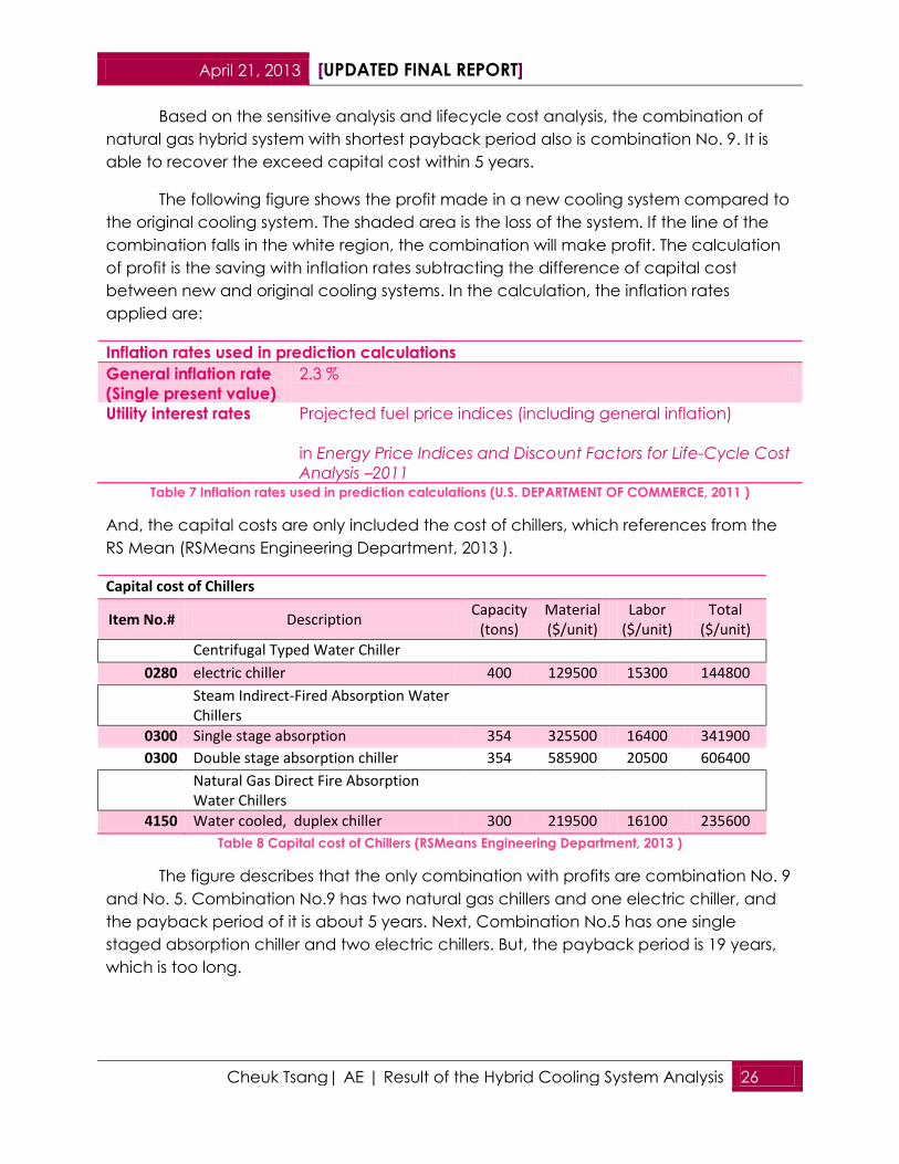
Based on the sensitive analysis and lifecycle cost analysis, the combination of
natural gas hybrid system with shortest payback period also is combination No. 9. It is
able to recover the exceed capital cost within 5 years.
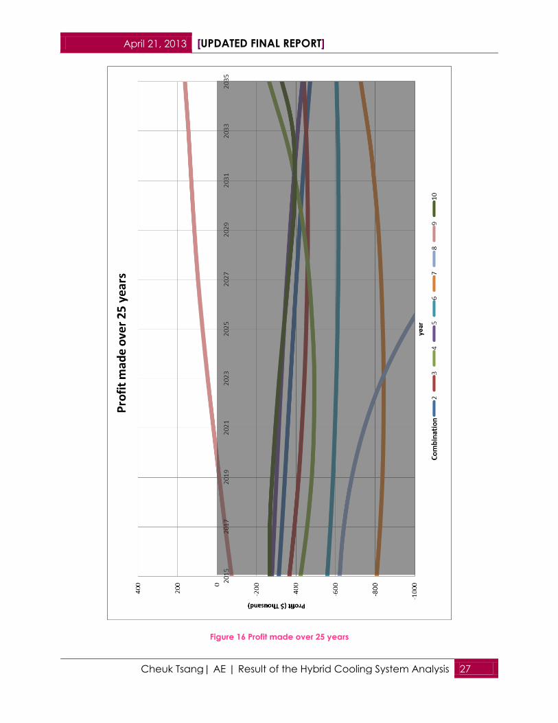
The following figure shows the profit made in a new cooling system compared to
the original cooling system. The shaded area is the loss of the system. If the line of the
combination falls in the white region, the combination will make profit. The calculation
of profit is the saving with inflation rates subtracting the difference of capital cost
between new and original cooling systems. In the calculation, the inflation rates
applied are:
Inflation rates used in prediction calculations
General inflation rate
(Single present value)
2.3 %
Utility interest rates Projected fuel price indices (including general inflation)
in Energy Price Indices and Discount Factors for Life-Cycle Cost
Analysis –2011 Table 7 Inflation rates used in prediction calculations (U.S. DEPARTMENT OF COMMERCE, 2011 )
And, the capital costs are only included the cost of chillers, which references from the
RS Mean (RSMeans Engineering Department, 2013 ).
Capital cost of Chillers
Item No.# Description Capacity
(tons) Material ($/unit)
Labor ($/unit)
Total ($/unit)
Centrifugal Typed Water Chiller
0280 electric chiller 400 129500 15300 144800
Steam Indirect-Fired Absorption Water Chillers
0300 Single stage absorption 354 325500 16400 341900
0300 Double stage absorption chiller 354 585900 20500 606400
Natural Gas Direct Fire Absorption Water Chillers
4150 Water cooled, duplex chiller 300 219500 16100 235600
Table 8 Capital cost of Chillers (RSMeans Engineering Department, 2013 )
The figure describes that the only combination with profits are combination No. 9
and No. 5. Combination No.9 has two natural gas chillers and one electric chiller, and
the payback period of it is about 5 years. Next, Combination No.5 has one single
staged absorption chiller and two electric chillers. But, the payback period is 19 years,
which is too long.
April 21, 2013 [UPDATED FINAL REPORT]
Cheuk Tsang| AE | Result of the Hybrid Cooling System Analysis 27
Figure 16 Profit made over 25 years

April 21, 2013 [UPDATED FINAL REPORT]
Cheuk Tsang| AE | Result of the Hybrid Cooling System Analysis 28
Natural Gas Hybrid System vs. Electric Cooling System
Combination No. 9 is the best of overall combinations. It is because the price of
natural is cheaper than the price of electricity now and in the future. The reason why
the HVAC engineers may neglect this selection is that it is difficult to compare the prices
of these two utility with different utility companies. Also, the calculation of these two
utility cost is tedious, since the structure of utility cost calculation and the cost itself are
changed every few years. In order to predict the future utility cost of a particular
company, it requires historical rates of several years, which sometimes isn’t opened to
public. Therefore, the extra cost of natural gas fired chiller can be made up within 5
years.
Natural Gas Hybrid System vs. Steam Hybrid System
The natural gas hybrid system in this analysis is more energy efficient and
cheaper than the steam hybrid system, because
A natural gas fired absorption water chiller is cheaper than both single and
double staged steam absorption chillers.
Cost Different Between Natural Gas and Steam Absorption
Chillers
Chiller types Cost ∆ %
Natural gas direct-
fired
(300 tons)
$ 235,600 ---
Single stage
indirect fired
(354 tons)
$ 341,900
+45%
Double stage
indirect fired
(354 tons)
$ 606,400 +157%
Table 9 Cost different between natural gas and steam absorption chillers
The coefficient of performance (COP) of natural gas chiller is higher.
Coefficient of Performance of Natural Gas and Steam
Absorption Chillers
Chiller types Coefficient of Performance
Natural gas direct-fired
(300 tons) 1.01
Single stage indirect fired
(354 tons)
0.7
Double stage indirect fired
(354 tons) 1.23
Table 10Coefficient of Performance of Natural Gas and Steam Absorption Chillers

April 21, 2013 [UPDATED FINAL REPORT]
Cheuk Tsang| AE | Result of the Hybrid Cooling System Analysis 29
Steam Hybrid System vs. Electric Cooling System
The reasons why the combinations with steam chillers are not economical are:
AAM will not be eligible for Steam Air-Conditioning Summer Discount Program,
because AAM is only eligible for No.1 steam rate.
Both single and double staged steam absorption chillers have too low COPs,
because the COP of an electric chiller is 0.63.
Since waste heat steam provides low quality heat, the system requires relatively
large amount.
Due to the difference of COPs, the makeup water consumption of cooling
towers.
Steam Hybrid Systems - Double Staged vs. Single Staged Absorption Chiller
Although both sets of combinations are unable to overcome the original system,
Combination No.1, the result shows that the combinations with single staged absorption
chillers is more economical than the ones with double staged absorption. It is because
the capital cost of a double staged absorption chiller is 100% higher than the cost of
single staged absorption chiller. And, the Incentive Program of Steam Cooling System
only covers 20% of the capital cost of a double staged steam absorption chiller, which
is not enough to recover both capital cost by lowered steam usage.
0
500
1000
1500
2000
2500
3000
3500
4000
4500
5000
1 2 3 4 5 6 7
Wa
ter
co
nsu
mp
tio
n (
1000 g
als
)
Combination
Water combination between original
system and steam hybrid system
water combination

April 21, 2013 [UPDATED FINAL REPORT]
Cheuk Tsang| AE | Change of Cooling System Needed to Adopt the New
Chiller
30
Change of Cooling System Needed to Adopt the New Chiller This section ensures if the characteristic of the best combination, No. 9, is able to
work well in the cooling system of AAM without damaging other components. And, the
information of original cooling system is provided by the mechanical drawing given by
AAM. Then, the information of combination No. 9 is recommended from Trane website.
It is because the characteristic of an absorption chiller in Trane website can well match
with the energy stimulation of Trace 700, which is the product of Trane. If the new chiller
doesn’t match the parameter of system, the change of system or chillers will be
needed.
Performance data comparison between electric and Trane natural gas chiller.1
Chiller Type Electric centrifugal
chiller
Trane natural gas absorption
chiller
Cooling Capacity
(Ton)
300 321
Heating Capacity
(MBH)
-- 2799.3
Refrigerant R134-a Absorbent: Lithium Bromide
(LiBr)
Refrigerant: Water
Dimension
(in) 172(L)x67(W)x82.1(H) 187.4(L)x113.4(W)x111.4(H)
Operating weight
(lbs.) 22436 27800
Ch
ille
r
Flow rate
(GPM ) 450 777.1
Inlet water
temperature (oF)
58 54
Outlet water
temperature (oF)
42 44
Max. pressure drop
(ft. H2O)
8.9 25.6
Number of passes 2 2
Co
nd
en
ser
Flow rate
(GPM ) 900 1391.3
Inlet water
temperature (oF)
85 85
Outlet water
temperature (oF)
95 94.46
Max. pressure drop
(ft. H2O)
17 22.3
Working pressure (Psig) 150 --
Number of passes 2 Absorber: 2
Condenser: 1

April 21, 2013 [UPDATED FINAL REPORT]
Cheuk Tsang| AE | Change of Cooling System Needed to Adopt the New
Chiller
31
Performance data comparison between electric and natural gas chiller.1
Ele
ctr
ica
l
kW (Power factored) 195 --
Voltage 208 460
Phase 3 3
Frequency 60 60
kW/ton .6 --
Total full load Amp 631 10.6
Table 11 Performance data comparison between electric and Trane natural gas chiller.1
In this comparison, the highlighted rows show the major differences between two
chillers.
Different Refrigerants
Both chiller types consist of different refrigerants. The electric chillers of AAM
contain a safer refrigerant, R134a, and a natural gas fired chiller has lithium bromine as
an absorbent and water as a refrigerant. However, lithium bromide is a corrosive
solution, so it is requires an extra sensor and stricter mechanical room design for safety
purposes. Therefore, the catalog referenced from Trane mentions a built-in inhibitor and
a design suggestion of a mechanical room, which is similar to ASHRAE Standard 15—
Safety Standard for Refrigeration Systems (Thermax Ltd. ).
The absorption chiller of Trane has a built-in corrosion inhibitor, lithium molybdate,
and factory mounted on-line purging system. The on-line purging system is to
purge any non-condensable gas into a storage tank to keep the corrosion rates
low.
The following table shows the major consideration of mechanical room layout.
Machine room layout consideration
Electrical All conductors should be made of copper.
Piping
Far gas fire system, the piping design pressure should be higher than the
operation pressure.
The piping should be installed with a stop valve, safety device, drain and
sampling connections.
If a cooling water pump is not installed with each chiller, this chiller should
be connected with an auto-operated butterfly valve.
Control
system
The chiller control panel should interlocking chilled water and cooling water
of the absorption chiller. Table 12 Machine room layout consideration (Thermax Ltd. )
ASHRAE Standard 15 states that
o The door of the chiller room should be tight-fitting and opened outward.

April 21, 2013 [UPDATED FINAL REPORT]
Cheuk Tsang| AE | Change of Cooling System Needed to Adopt the New
Chiller
32
o There should be refrigerant sensors. The sensors should be located where
refrigerant concentrates and coupled to alarm and mechanical
ventilation.
o The purge system and its relief must be vented outside, minimum 20 ft.
away from ventilation openings and minimum 15 ft. above ground.
Different Flow Rates
In the comparison, the GPMs of both chillers are different. Therefore, the valves
of the new chillers must be resized in order to handle bigger amount of flow. The
following figure illiterates the new cooling system with two natural gas chillers, and the
circled components are required resizing. The changes of cooling system are not
significant, because the chosen absorption chillers are designed for variable frequency
control. And also, the original piping system is Primary/Secondary Variable flow piping
designed. This system is “desirable to have the flow rate in primary loop equal to or
greater than the flow rate in the secondary loop”. (Vogelsang, 2000)Although the
natural gas chillers provide much higher flow rate, the flow can be regulated by the
piping loop. Moreover, if needed, a new bypass between returning and supplying
chilled water to load will be added.

April 21, 2013 [UPDATED FINAL REPORT]
Cheuk Tsang| AE | Change of Cooling System Needed to Adopt the New
Chiller
33
New bypass
Valves needed resizing
April 21, 2013 [UPDATED FINAL REPORT]
Cheuk Tsang| AE | Change of Cooling System Needed to Adopt the New
Chiller
34
Figure 17 New cooling system of Combination No. 9
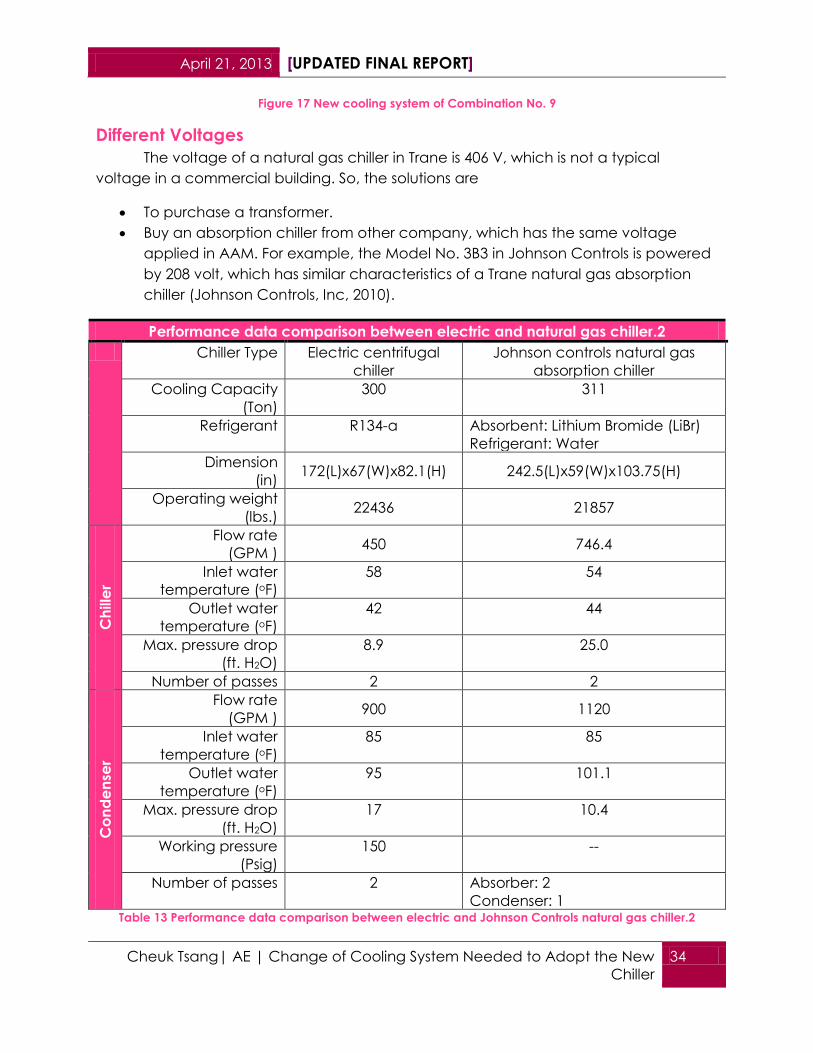
Different Voltages
The voltage of a natural gas chiller in Trane is 406 V, which is not a typical
voltage in a commercial building. So, the solutions are
To purchase a transformer.
Buy an absorption chiller from other company, which has the same voltage
applied in AAM. For example, the Model No. 3B3 in Johnson Controls is powered
by 208 volt, which has similar characteristics of a Trane natural gas absorption
chiller (Johnson Controls, Inc, 2010).
Performance data comparison between electric and natural gas chiller.2
Chiller Type Electric centrifugal
chiller
Johnson controls natural gas
absorption chiller
Cooling Capacity
(Ton)
300 311
Refrigerant R134-a Absorbent: Lithium Bromide (LiBr)
Refrigerant: Water
Dimension
(in) 172(L)x67(W)x82.1(H) 242.5(L)x59(W)x103.75(H)
Operating weight
(lbs.) 22436 21857
Ch
ille
r
Flow rate
(GPM ) 450 746.4
Inlet water
temperature (oF)
58 54
Outlet water
temperature (oF)
42 44
Max. pressure drop
(ft. H2O)
8.9 25.0
Number of passes 2 2
Co
nd
en
ser
Flow rate
(GPM ) 900 1120
Inlet water
temperature (oF)
85 85
Outlet water
temperature (oF)
95 101.1
Max. pressure drop
(ft. H2O)
17 10.4
Working pressure
(Psig)
150 --
Number of passes 2 Absorber: 2
Condenser: 1 Table 13 Performance data comparison between electric and Johnson Controls natural gas chiller.2

April 21, 2013 [UPDATED FINAL REPORT]
Cheuk Tsang| AE | Change of Cooling System Needed to Adopt the New
Chiller
35
Different Dimensions
The dimension difference of the electric chiller and the absorption chillers is
significant.
Dimension of different chillers
Dimension
Electric Chiller Trane Absorption
Chiller
Johnson Controls
Chiller
Length 172 187.4 242.5
Width 67 113.4 59
Height 82.1 111.4 103.75 Table 14 Dimension of different chillers
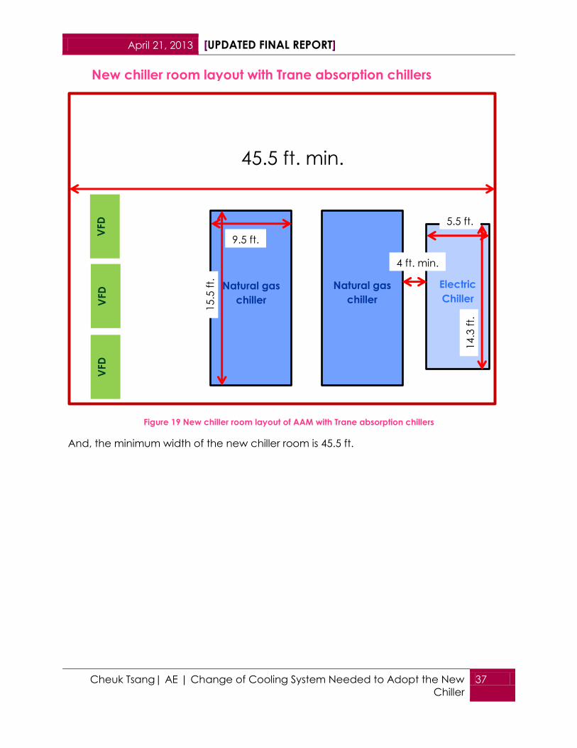
Luckily, the height of chiller room is 20 ft., which is tall enough to hold the natural gas
chillers. But, the width of new chillers may cause the width or length of chiller room to
increase, due to accessibility and the recommendation of the Trane absorption chiller
catalog. It says that
The clearance space on all sides of chiller should be at least 3.3 ft.
The clearance on the panel side of the chiller should be at least 3.95 ft.
The space above the chiller should be more than 0.7 ft.

April 21, 2013 [UPDATED FINAL REPORT]
Cheuk Tsang| AE | Change of Cooling System Needed to Adopt the New
Chiller
36
Figure 18 Original chiller room of AAM
42.5 ft.
35.5 ft.
VFD
s 4
3.7
ft.
VFD
s V
FD
s
Chiller Chiller Chiller
Original chiller room layout
April 21, 2013 [UPDATED FINAL REPORT]
Cheuk Tsang| AE | Change of Cooling System Needed to Adopt the New
Chiller
37
Figure 19 New chiller room layout of AAM with Trane absorption chillers
And, the minimum width of the new chiller room is 45.5 ft.
VFD
V
FD
V
FD
Natural gas
chiller
Natural gas
chiller
Electric
Chiller
4 ft. min.
9.5 ft.
15
.5 f
t.
5.5 ft.
14
.3 f
t.
45.5 ft. min.
New chiller room layout with Trane absorption chillers

April 21, 2013 [UPDATED FINAL REPORT]
Cheuk Tsang| AE | Change of Cooling System Needed to Adopt the New
Chiller
38
Table 15 New chiller room layout with Johnson Controls absorption chillers
The size of original mechanical room doesn’t need to be changed, because the
minimum width is achieved.
VFD
V
FD
VFD
Natural gas
chiller
Natural gas
chiller
Electric
Chiller
4 ft. min.
5 ft.
20
ft.
5.5 ft.
14
.3 f
t.
38.5 ft. min.
New chiller room layout with Johnson Controls absorption chillers

April 21, 2013 [UPDATED FINAL REPORT]
Cheuk Tsang| AE | Analysis of Operation Sequences for Hybrid System 39
Analysis of Operation Sequences for Hybrid System
Purpose
Since the analysis of hybrid system results the most cost efficient system is the
combination of natural gas hybrid system with two natural gas chillers and one electric
chiller. And, the following study is to seek for the most cost effective operation of
sequence. This study is inspired by a question asked in Architectural Engineering Thesis
Capstone Project presentation related to the sequence of chiller operation. The search
method of the operation sequence study is the same with the search method of the
pervious analysis. It is because it significantly reduces the time consumption of
calculation and brain storming.
Analysis of Operation Sequence
This section describes the setup of energy model and the result of the
stimulations. The energy model was built on the model of the most cost effective hybrid
system found in the previous analysis. In this analysis, there are 7 types of operation
sequences studied.
Progress of Building Energy Model and Calculating Annual Utility Cost
Setup and Assumptions Energy Model
According to the assumption, because the energy model was built based on the
energy model of the hybrid system combination, 2 natural chillers and 1 electric chiller,
the same assumption also are kept in the model except the sequence of operation.
Next, the default characteristics of both chillers are also kept in this model, due
to lack of information. It is difficult In Trace 700, the 2 models of chillers are
90.1-04 Min Centrifugal 150-300 tons as the electric chiller
Direct Fired Absorption – Horizon as the two natural gas absorption chillers
Both chillers are set that the power consumption and the load ratio are linearly
proportional.

April 21, 2013 [UPDATED FINAL REPORT]
Cheuk Tsang| AE | Analysis of Operation Sequences for Hybrid System 40
Figure 20 Power consumption vs. full load of a Trace 700 electric chiller model
Figure 21 Power consumption vs. full load of a Trace 700 natural gas direct fired chiller model

April 21, 2013 [UPDATED FINAL REPORT]
Cheuk Tsang| AE | Analysis of Operation Sequences for Hybrid System 41
Annual Utility Cost
The annual utility costs of each sequence over 20 years are conducted. The
data of energy consumption is inputted into the calculation of utility cost prediction
with utility regression equations. The regression equations of natural gas and water are
the same set of pervious study, and the electricity is generated with the same
approach, which the regression equation is generated by the annual electricity cost
from 2004 to 2012, instead of every item of a utility cost.
Operation Sequences of the Hybrid System Studied
There are 7 sequences of chiller operation studied in this analysis.
No. 1 Chillers Operating in Parallel
Figure 22 No.1 Chillers in Parallel
This sequence allows the chillers running at all the time mostly part load.

April 21, 2013 [UPDATED FINAL REPORT]
Cheuk Tsang| AE | Analysis of Operation Sequences for Hybrid System 42
No. 2 Chillers Operating in Single
Figure 23 No.2 chillers in single
This sequence is to operate the electric chiller first, until the capacity of the
electric chiller is reached. Then, one of the natural gas chillers will be turned on, if the
capacity of the electric chiller is exceed.
No. 3 Chillers Operating in Single-2
Figure 24 No. 3 Chillers Operating in Single-2
This sequence is similar to the No.2 sequence, but the first chiller starting is natural
gas direct fired absorption chiller.

April 21, 2013 [UPDATED FINAL REPORT]
Cheuk Tsang| AE | Analysis of Operation Sequences for Hybrid System 43
No. 4 Electric Chiller Operating in Sidecar
Figure 25 No. 4 Electric Chiller Operating in Sidecar
This sequence is required no valves and the flow in bypass is driven by the
pressure difference. The electric chiller in the sequence is in the Sidecar sequence.
No. 5 Natural Gas Chiller Operating in Sidecar
Figure 26 No. 5 Natural Gas Chiller Operating in Sidecar
In this sequence, a natural gas chiller in the sequence is in the Sidecar sequence.

April 21, 2013 [UPDATED FINAL REPORT]
Cheuk Tsang| AE | Analysis of Operation Sequences for Hybrid System 44
No. 6 Chillers in Decouple Parallel
Figure 27 No. 6 Chillers in Decouple
This sequence is that all three chillers operate all the time. And, the cooling load
is evenly distributed, since the tonnage of each chiller is the same. The water flow
through the electric chiller first.
No. 6 Chillers in Decouple Parallel-2
Figure 28 No. 6 Chillers in Decouple Parallel-2
This sequence is similar with Sequence No. 6. However, because there are two
types of chillers in this hybrid system, the water temperatures of evaporators and
condensers are also different. And, because the water flows through natural gas chiller

April 21, 2013 [UPDATED FINAL REPORT]
Cheuk Tsang| AE | Analysis of Operation Sequences for Hybrid System 45
first, the result of energy consumptions between Sequence No. 6 and No. 7 are
different.
Result of Operation Sequence Analysis
By comparing the payback period (Figure. 29), it shows the best operation
sequences are
No. 1 Chillers Operating in Parallel.
All the chillers operate with evenly load during all the time.
No. 2 Chillers Operating in Single.
The electric chiller operates first until it reaches its full capacity.
No. 6 Chillers Operating in Decouple.
The chillers operate with load proportional to the capacity of each chiller.
Figure 29 Payback Period of Operation Sequence

April 21, 2013 [UPDATED FINAL REPORT]
Cheuk Tsang| AE | Analysis of Operation Sequences for Hybrid System 46
Conclusion
The result shows that the most cost effective operation sequences are:
Parallel.
The chillers operate with evenly distributed load.
Single.
The electric chiller operates first, than the natural gas chiller start operating.
There are suggestions of operation sequences. Because it is difficult to obtain the IPLV
data of a chiller in the catalog of manufacturer, the decision of selecting the suitable
operation sequence cannot be made without the corresponding IPLA data of the
selected chillers.
The decoupling piping system is needed. Since the analysis of hybrid system
concludes that the flow rates of both chillers are very different, a bypass should be
placed between return and supply pipelines. This approach is similar to the decoupling
piping system. The decouple system is used to solve the pressure and temperature
differences between the components in a mechanical system.
Between the chillers operating in single and parallel, it should be based on
efficiency at part load. Some of the chillers have relatively high efficiency at part load,
and some are more efficient at full load. It is important to understand the energy
consumption of a chiller under different ratio of load. Since the characteristic of
Johnsons’ Control Chiller is that the efficiency also is linearly proportional to the design
load, it suggests the single in decoupling piping system is a better choice.
Figure 30Energy consumption vs load of a Johnsons' Control Chiller
However, it is important to input the IPLV data into the energy model stimulation in order
to ensure the potential saving.

April 21, 2013 [UPDATED FINAL REPORT]
Cheuk Tsang| AE | Economic Analysis 47
Economic Analysis
Current Condition of Utility Rate
Based on the current condition, the rate of electricity is increasing significantly,
because the fuel of major power plants in ConEdison is oil and the prices of No. 2 and 6
oils are increasing. And, the rate of natural gas is more still and stable. It is because the
shale technology is well developed to supply a reliable amount of supply nowadays.
Figure 31 Con Edison’s Citygate Cost of Gas for Firm Customers Versus #2 & #6 Oil (ConEdison , 2010 )
In the website of ConEdison, there are several reasons why ConEdison would like to
generate power with oil fueled power plants.
“While natural gas is currently the less expensive fuel, it has not always
been so. There have been times when oil was less expensive than natural
gas.”
“During the winter season, there are some days when natural gas is in
short supply. When natural gas is in short supply, it must be given to Con
Edison’s gas customers before any is used in Con Edison’s own facilities.”
“Because Con Edison has the capability to produce steam from two
different fuels, Con Edison can reliably produce steam at the best price.”
---- ConEd (Con Edison, 2012)

April 21, 2013 [UPDATED FINAL REPORT]
Cheuk Tsang| AE | Economic Analysis 48
It is less likely that the electric price will decrease, if the current condition of the
ConEdison power generation system remains the same.
Future Plant of ConEdison Power Generation and Other Utilities
The biggest problem of a hybrid system is high sensitivity of utility cost. It is difficult
to predict the future utility cost throughout the lifetime of a chiller precisely. ConEdison is
planning to switch the fuel type of power generation system and promote CHP
(Combined Heat and Power) System. The main advantage of CHP toward the utility
company is the stable and consistent amount of demanded fuel over time.
Currently, the power plants are fueled by oil and back up with natural gas. In the
Gas Long Range Plan, 2010-2030, of ConEdison, it shows that ConEdison is willing to
switch the fuel of major power plants from No. 2 and 6 to natural gas. And, all the
power plants are switchable from oil to natural gas. But, this report doesn’t state clearly
about when or how the power plants operate with different fuels.
ConEdison is planning to change the fuel of power plant, because of two reasons:
The price of natural gas is decreasing in the future 30 years. And, the prices of
No. 2 and 6 oils have gone over the price of natural gas.
The NOx RACT regulation will be settled and limit the NOx emission from buildings
and facilities. One of the alternative solutions is to switch the fuel type of the
major power plants.
There are also drawbacks of changing fuels:
Since ConEdison planned to change the fuel of power plant, it will lower the
production of steam. In order to balance the demand and supply of steam,
ConEdison plans to start incentive program to convince the steam customers to
replace steam heating system with natural gas CHP (Combined Heat and
Power) system. But, a CHP system consists of high capital cost and stable thermal
load profile. ConEdison will require big amount of funding to convince the steam
customer.
In the Gas Long Range Plan of ConEdison, it shows that if the power generation
system switches the fuel type, the load will be increased by 400 thousand
dekatherms per day (Mdt/day).
According to the damage of Sandy, ConEdison seeks for $400 million from
customers to repair the damage of Sandy and prepare for the natural disaster in
future. ConEdison will increase the rate of natural gas by 1.3 percent and the
rate of electricity by 3.3 percent. Since the electric delivery system received
April 21, 2013 [UPDATED FINAL REPORT]
Cheuk Tsang| AE | Economic Analysis 49
more damage from Sandy, the funding requested will be more and used for
“increase the height of flood walls for certain facilities; raise the level of critical
equipment; install submersible equipment; install additional switches and related
smart grid technology; and reconfigure certain distribution networks.”
(McGeehan, 2013) And, the funding corresponding to natural gas will be used
for “the connection to a new gas transmission pipeline, projects for cover plates
and remote emergency generators to address possible tunnel flooding and
check valves to prevent water infiltration that could lead to over-pressurization of
piping and equipment.” (McGeehan, 2013)
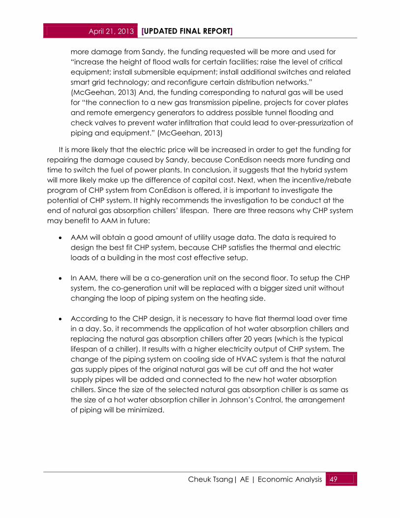
It is more likely that the electric price will be increased in order to get the funding for
repairing the damage caused by Sandy, because ConEdison needs more funding and
time to switch the fuel of power plants. In conclusion, it suggests that the hybrid system
will more likely make up the difference of capital cost. Next, when the incentive/rebate
program of CHP system from ConEdison is offered, it is important to investigate the
potential of CHP system. It highly recommends the investigation to be conduct at the
end of natural gas absorption chillers’ lifespan. There are three reasons why CHP system
may benefit to AAM in future:
AAM will obtain a good amount of utility usage data. The data is required to
design the best fit CHP system, because CHP satisfies the thermal and electric
loads of a building in the most cost effective setup.
In AAM, there will be a co-generation unit on the second floor. To setup the CHP
system, the co-generation unit will be replaced with a bigger sized unit without
changing the loop of piping system on the heating side.
According to the CHP design, it is necessary to have flat thermal load over time
in a day. So, it recommends the application of hot water absorption chillers and
replacing the natural gas absorption chillers after 20 years (which is the typical
lifespan of a chiller). It results with a higher electricity output of CHP system. The
change of the piping system on cooling side of HVAC system is that the natural
gas supply pipes of the original natural gas will be cut off and the hot water
supply pipes will be added and connected to the new hot water absorption
chillers. Since the size of the selected natural gas absorption chiller is as same as
the size of a hot water absorption chiller in Johnson’s Control, the arrangement
of piping will be minimized.

April 21, 2013 [UPDATED FINAL REPORT]
Cheuk Tsang| AE | Overall Conclusion 50
Overall Conclusion This analysis is to seek a hybrid system with the variation of fuel types. It found
that the combination No. 9 with two natural gas chillers and one electric chiller is more
economical than the original cooling system, because the natural gas price is cheaper
than the price of electricity nowadays. As a conclusion, it is presented in 2 ways:
technical and economical perspectives.
Technical Conclusion—Why Natural Gas Fired Absorption Chillers?
This section is about pros and cons of the combination No. 9.
One of the reasons that the natural gas hybrid system is more economical in
AAM than the electric cooling system and the steam hybrid system are that the price of
natural gas is getting lower. It is caused by the supply in shale gas in United States is
increasing recently. The technology of collecting shale gas is becoming more
economical. As the cost of natural gas extraction is more, the supply of natural gas
increases. Comparing to the COP of all chillers, although the COP of natural gas fired
absorption chiller is lower than the electric chiller, it is higher than the one of steam
absorption chiller. It is because the steam in double and single staged absorption
chillers cannot carry a lot of heat. Also, the power plant of ConEdison produces low
quality of heat. Therefore, using natural gas fired absorption chillers is a better choice.
The impact of this hybrid system is that the size of an absorption chiller is at least
25 % larger than an electric chiller. It may cause the size of a chiller room to increase
due to the minimum clearance. The other solution is to select an optimal size of chiller.
However, in this energy analysis, it is not conducted with the preferred chiller, but a
Trane absorption chiller. It is because Trace700 is design for operating with Trane
equipment. When a chiller of other brand is used, the built-in function should be
modified in Trace700, such as integrated part load values, for matching the load
characteristics.
As conclusion, the preferred natural gas chiller has similar characteristics with the
Trane chiller and optimal size. So, this hybrid system doesn’t impact the cooling system
significantly. Next, based on the analysis of operation sequence, it recommends the
application of “single in decoupling” sequence for minimizing the weariness of the
equipment and maximizing the cost effectiveness of it.

April 21, 2013 [UPDATED FINAL REPORT]
Cheuk Tsang| AE | Overall Conclusion 51
Economical Conclusion—Price of Natural Gas and Future Plan of AAM
Mechanical System
After conducting an economic study, there are one conclusion and one
suggestion of the future mechanical system in AAM:
Hybrid system is recommended due to the current fuel economic condition.
The potential of CHP system should be investigated in the end of the
absorption chiller lifespan.
These two ideas are based on the short term and long term predictions of ConEdison
utility system and plans.
Short term economic prediction
According to Gas Long Range Plan of ConEdison, the rate of electricity remains
high and the natural gas costs lower in these recent years. It is because the price of oil is
increasing, and the shale gas technology is well developed that increases the amount
of natural gas supply. It results that the hybrid system is recommended.
Long term economic prediction
The report of ConEdison’s plan states that in next 30 years, ConEdison invests on
expanding the natural gas delivery system and promoting the natural CHP system. In
these 30 years, the supply and demand of natural gas will be balance. Therefore, the
consideration of CHP system is suggested to be the replacement of hybrid system.
This economic analysis does not require the long term prediction. However, the
prediction can provide the owner better and greener ideas of the future mechanical
system.

April 21, 2013 [UPDATED FINAL REPORT]
Cheuk Tsang| AE | Purposes 52
Structural and Acoustical Breadths--
New Mechanical Ductwork Layout
Purposes The mechanical area in AAM will be around 1/3 of gross area, because there will
be 3 mechanical floors in AAM. Two out of three floors will hold the major equipment of
cooling, heating and ventilation systems, then another floor will locate the
cogeneration system. The main idea in this analysis is to seek for capital saving of
ductwork by relocating a part of the ventilation systems in two floors with the
consideration of structural and acoustical impact. The approach of this analysis is to
increase the size of ventilation system on 9th floor and lower the capacity of the one on
cellar level in order to minimize the amount of ductwork.
Design Criteria In this section, it states the existing conditions of the current mechanical
ductwork layout.
Placement of Mechanical Equipment
The 3 mechanical floors will be:
Mechanical floor Mechanical room(s) and equipment located in this floor
Cellar level Chiller room
Boiler room
Ventilation systems serving cellar level to 7th floor
2nd floor Cogeneration System room
9th floor Ventilation systems serving 8th floor Table 16 Location of Mechanical rooms and equipment
As the table shown, the major equipment will be located in the cellar level. And, the
longest ductworks will be the ones of supplying and returning the conditioned air from
7th floor to cellar level.
Redundancy of Ventilation Systems in AAM
This analysis is focused on the major air condition systems, which will serve the
gallery and office zones throughout the whole buildings. There will be three 42000 cfm
AHUs (air handling units) on cellar level that will supply and return the air up to 7th floor,
then only 1 AHU on 9th floor. Therefore, if the ventilation system on 9th floor is shut down
due to maintenance and equipment failure, 8th floor will not have conditioned air
served.

April 21, 2013 [UPDATED FINAL REPORT]
Cheuk Tsang| AE | Proposed Air Handling Unit Locations and Ductwork Layout 53
Structural System of AAM
The structural system of AAM will be a partially composited steel system. The
beam which will support the weight of façade will be a composite beam, and most of
the column in AAM also will be a composite column.
Acoustical control of AAM
In AAM, there will be noise sensitive rooms, such as a classroom and a theater.
Therefore, the mechanical equipment will be specifically selected based on sound
level.
On 8th floor, every fan power VAV unit will be installed with a sound trap.
In the specification of AAM, all fans, diffusers and VAV boxes must operate
below the maximum sound level.
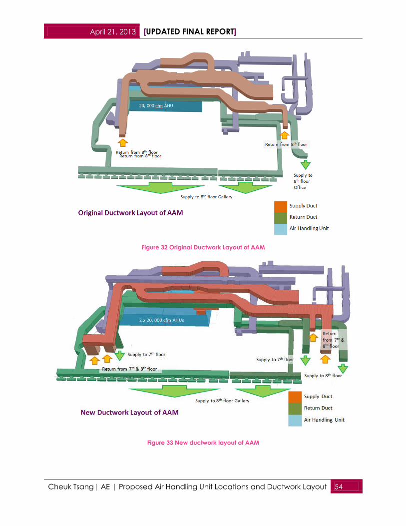
Proposed Air Handling Unit Locations and Ductwork Layout The proposed air handling units and the location are two 50,000 cfm AHUs in
cellar level and two 20,000 cfm AHUs on 9th floor. The considerations that this
combination is picked are:
Having two AHUs on each mechanical floor provides better reliability.
Since the usable area of 9th floor is limited, two units of AHUs are the maximum
number of AHUs, which can be located on 9th floor.
The two 50,000 cfm AHUs will serve the galleries and offices from cellar level to 6th floor,
and the other two 20,000 cfm AHUs will supply and return the air to 7th and 8th floors. To
avoid unnecessary structural and acoustical change, the addition supply and return
ducts on 9th floor that will deliver conditioned air to 7th floor should be connected to the
original supply and return ducts. As the original ducts that will send air to 7th floor from
cellar level will be cancelled in this analysis, the return and supply ducts on 7th floor will
be expanded to 9th floor. Therefore, the length of ductwork saved will be at least160
feet.
April 21, 2013 [UPDATED FINAL REPORT]
Cheuk Tsang| AE | Proposed Air Handling Unit Locations and Ductwork Layout 54
Figure 32 Original Ductwork Layout of AAM
Figure 33 New ductwork layout of AAM

April 21, 2013 [UPDATED FINAL REPORT]
Cheuk Tsang| AE | Result with 3 perspectives: Mechanical, Structural and
Acoustical
55
Result with 3 perspectives: Mechanical, Structural and Acoustical The result of 3 analyses (duct sizing, structural system check and acoustical
performance stimulation) shows that moving an AHU to 9th floor reduces the capital
cost of ductwork by $36,000 without causing structural and acoustical impacts.
Mechanical Perspective
By changing the ventilation distribution, the capital cost of ventilation system
decreases.
After moving an AHU to 9th floor, the size of ductworks is reduced, because of
decreasing the pressure drop in the ductwork. Also, it increases the amount of piping,
which the pipes of chilled water supply and return and the pipes of hot water supply
and return. The reason why shifting the AHUs closed to the loads is that the cost of
ductwork is greater than the cost of piping.
Capital Cost Analysis
Cost lost Cost gained
Item Quantity Cost/unit Cost Item Quantity Cost/unit Cost
AHUs AHUs
AHU 42,000 cfm 3 74500 223500 AHU 50,000 cfm 2 96000 192000
AHU 20,000 cfm 1 37100 37100 AHU 20,000 cfm 2 37100 74200
Duct Duct
Cellar Level 128851.3 Cellar Level 22501.54
9th floor 9880.043 9th floor 70583.48
Pipe Pipe
9th floor 3550
Total Total
399331.34 362835.02
Saving (Cost lost - Cost gained)
36496.32 Table 17 Capital Cost Analysis
According to Table.17, the saving is about $36,000.
Also, it increases redundancy of the ventilation on 9th floor. It is because if either
one of the AHUs on a floor fails, the second AHU will still operate and provide minimum
air flow.

April 21, 2013 [UPDATED FINAL REPORT]
Cheuk Tsang| AE | Result with 3 perspectives: Mechanical, Structural and
Acoustical
56
Structural Perspective
Since a ~9,000 pounds weighted AHU will be moved to the 9th floor, it may affect
the building structural load. It is required to check the capacity of the major structural
components: composite deck, beams, and columns.
In the structural system check, the load distribution based on the drawings and
the calculated weight of AHUs and other ventilation equipment is the following:
Table 18 Load distribution calculation
Next, the area of 9th floor conducted in this check is:
Figure 34 Area of 9th floor conducted in this check
The structural check shows that the major structural components are all capable to
support the additional structural load. Finally, there is an additional check by applying
the point load to the columns under the AHUs in the calculation. And, all the columns
also achieve the minimum load requirement.
Loads Load distribution
live load 75 psf from drawing
ductwork and pipe 15 psf
Steel 12 psf
equipment weight quantiity total
lbs lbs
fan 1000 3 3000
AHU 9000 2 18000
HVs 1500 3 4500
total 25500 lbs
total/total area 5.73 psf
total distributed load 107.73 psf
Mechanical equipment load
Load distribution calculation

April 21, 2013 [UPDATED FINAL REPORT]
Cheuk Tsang| AE | Result with 3 perspectives: Mechanical, Structural and
Acoustical
57
Acoustical Perspective
The acoustical performance should be checked and ensured if the minimum
noise criteria (NC) are achieved. Also, as the duct is resized, the sizing should follow the
‘Rules of Thumb” (McQuiston, 2005):
The air velocity in each duct should be less than 2400 fpm
The pressure drop must also be less than 0.1 in. wg.
It prevents turbulence flow inside the duct and minimizes the noise generation.
The galleries on 7th & 8th floors and the office areas (Rm 803 and Rm 703) on
these two floors with the shortest flanking path should conducted in acoustical
performance stimulation. The result shows that the noise generated by the AHUs is
mostly dissipated inside the ducts before the air reaching the diffuser. The loudest noise
generated and reaching out of the diffuser is from a fan powered VAV units with sound
trap. After leaving from a sound trap, the noise will be high frequency sound. Next,
when the noise leaves from the diffusers and reach to the ceiling, gypsum board tiles,
the high frequency noise is dissipated inside the tiles. It reduces the noise on 8th floor
below the minimum NC value.

April 21, 2013 [UPDATED FINAL REPORT]
Cheuk Tsang| AE | Result with 3 perspectives: Mechanical, Structural and
Acoustical
58
The acoustical performance of Rm703, opened office
Figure 35 Acoustical performance before fan powered VAV box
Acoustical performance of Rm 803 and Rm 805, opened office
Figure 36 Acoustical performance before fan powered VAV box

April 21, 2013 [UPDATED FINAL REPORT]
Cheuk Tsang| AE | Conclusion 59
Conclusion Having multiple floors of “Mechanical floor” is unusual, because it reduces the
usable space of the building. But, the application of mechanical floor brings the AHU
closer to the load, which decreases the amount of ducts. In AAM, there will be 3
mechanical floors. And, the engineer brought the AHU of serving 8th floor ventilation
much closer to the load. In this analysis, the proposed idea is to bring more AHUs closer
to the load and increase the redundancy of the system.
Mechanical floor has several disadvantages. And, the proposed ductwork layout
in this report is focus on minimizing the side effect to the structural system and the
acoustical performance. Fortunately, after all the checks, it shows that the structure of
AAM will be capable to support the extra weight of an AHU. The columns of AAM will
be able to carry the weight of both new AHUs individually.
According to the acoustics treatment in AAM, the treatment is slightly over
designed. It is because after placing linings in the ducts on 9th floor, the sound level of
noise generated by AHUs decreases significantly. The NC value before reaching
another noise generated device is about 20.
As the conclusion, new placement of AHUs saves about $36,000 with the resized ducts
and piping. And, it will bring zero structural impact and no disturb of acoustical
performance.

April 21, 2013 [UPDATED FINAL REPORT]
Cheuk Tsang| AE | Conclusion 60
MAE Course Relation
The MAE courses related to this project are:
AE 557 Centralized Cooling System:
The ideas of absorption refrigeration in this course help to understand the impact to
other mechanical components and the installation requirement of absorption chillers.
Also, the lecture of AHRI Standard 550/590 and ASHRAE Standard 90.1 explains the
potential energy saving of operating with multiple chillers instead of one.
AE 555 Building Control System:
This course provides different search methods that can be applied on HVAC operation,
such as increasing the efficiency of HVAC system by changing the combination of mass
flow rates, temperature setpoints, and part load ratios. This concept helps to find the
cost effective combination of electric and absorption chillers, and also the well
balanced layout of the mechanical room on 9th floor.

April 21, 2013 [UPDATED FINAL REPORT]
Cheuk Tsang| AE | Works Cited 61
Works Cited HVAC Absorption Chillers vs Electric Chillers. (2012, July 1). Retrieved from HVAC System
, HVAC Water Chillers,Valves and Pumps: http://hvac-system-
basics.blogspot.com/2012/07/hvac-absorption-chillers-vs-electric.html
ANSI/ASHRAE/IESNA. (2007). ASHRAE Handbook. Atlanta, GA: American Society of
Heating Refrigeration and Air Conditioning Engineers, Inc.
ASHRAE. (2012). ASHRAE Handbook: HVAC Systems and Equipment . ASHRAE.
Blinds Chalet. (2012). Roller Shades - Roller Blinds - Roll Up Shades. Retrieved from Blinds –
Window Treatments - Window Blinds and Shades - Horizontal Blinds - Window
Shutters: http://www.blindschalet.com/window-shades/rollershades.html
Bureau of Labor Statistics. (2012). AVERAGE ENERGY PRICES IN NEW YORK-NORTHERN
NEW JERSEY – JUNE 2012 . New York, NY: NEW YORK – NEW JERSEY INFORMATION
OFFICE .
Con Edison. (2012). Con Edison. Retrieved from Con Edison: steam operations -
knowledge center: faqs: http://www.coned.com/steam/kc_faqs.asp
Con Edison of New York. (2011, 10 1). steam rates: rate schedules. Retrieved from Con
Edison of New York: http://www.coned.com/documents/steam/Historical-
Rates/Tariff_LeavesSCs_20111001.pdf
Con Edison of New York. (2012). energy efficiency - Targeted Demand Side
Management. Retrieved from Con Edison of New York:
http://www.coned.com/energyefficiency/steamac.asp
ConEdison . (2010 , December ). Natural Gas Watch.org » Natural Gas Watch. Retrieved
from http://www.naturalgaswatch.org/wp-content/uploads/2012/11/ConEd-
Gas-Long-Range-Plan-2010-2030.pdf
ConEdison . (2012, 10 01). Schedule for Gas Service, P.S.C. No. 9 – Gas. Retrieved from
Con Edison of New York: http://www.coned.com/documents/allrates.pdf
ConEdison. (2012, September 21). Consolidated Edison. Retrieved from Wikipedia, the
free encyclopedia: http://en.wikipedia.org/wiki/Con_Edison
ConEdison. (2013, 01 23). Con Edison Offers Plans to Protect Customers and Energy
Systems From Major Storms. Retrieved from ConEdison:
http://www.coned.com/newsroom/news/pr20130125.asp
April 21, 2013 [UPDATED FINAL REPORT]
Cheuk Tsang| AE | Works Cited 62
ConEdison Media Relations . (2013). CON EDISON OFFERS PLANS TO PROTECT
CUSTOMERS AND ENERGY SYSTEMS FROM MAJOR STORMS . Con Edison:
newsroom .
Consolidated Edison Company of New York, Inc. (2012, 02 20). Service Classifications
("SC"s). Retrieved from Con Edison: Rates and Tariffs - Electric Rates and Tariffs:
www.coned.com/documents/elecPSC10/SCs.pdf
Johnson Controls, Inc. (2010). YIA Single-Effect Absorption Chillers Steam And Hot Water
Chillers. Milwaukee, WI : Johnson Controls, Inc.
McGeehan, P. (2013). Utility Critics Seek Advocate for Customers in New York. The New
York Times , A24.
McQuiston. (2005). Heating, Ventilating, and Air Conditioning. NJ: John Wiley & Sons,
Inc. .
New York City Water Board . (2013). NYC Water Board - Rate Schedule. Retrieved from
NYC Water Board:
http://www.nyc.gov/html/nycwaterboard/html/rate_schedule/index.shtml
NYS Department of Public Service Electronic Tariff System. (2012). Effective Electric Tariff
Documents. Retrieved from NYS Department of Public Service Electronic Tariff
System:
https://www2.dps.ny.gov/ETS/search/searchShortcutEffective.cfm?serviceType=
ELECTRIC
RSMeans Engineering Department. (2013 ). RS Means, Mechanical Cost Data . Norwell
MA: Reed Construction Data Inc.
Smith, B. (2002). Economic Analysis of Hybrid Chiller Plants . ASHRAE Journal.
Spanswick, L. (2003). Advances in Steam Cooling. ASHRAE Journal.
Thermax Ltd. . (n.d.). EcoChill Direct Fired Vapor Absorption Chiller .
Trane. (2010). Use's Manual-Trace 700, Building Energy and Economical Analysis . Trane.
Trane. (2012). Trane Product Catalog, Earth Wise CenTraVac Water-Cooled Liquid
Chillers . Trane.
U.S. DEPARTMENT OF COMMERCE. (2011 ). Energy Price Indices and Discount Factors for
Life-Cycle Cost Analysis – 2011. Maryland : Applied Economics Office Engineering
LAboratory.

April 21, 2013 [UPDATED FINAL REPORT]
Cheuk Tsang| AE | Works Cited 63
U.S. Green Building Council. (2012). LEED 2009 for New Construction and Major
Renovations Rating System. Washington, DC: U.S. Green Building Council.
US Environmental Protection Agency. (2012, August 23). Summary of the Clean Water
Act. Retrieved from US Environmental Protection Agency:
http://www.epa.gov/regulations/laws/cwa.html
Vogelsang, M. (2000). CoolTools Chilled Water Plant Design and Specification Guide .
San Grancisco, CA : Pacific Gas and Electric Company .

April 21, 2013 [UPDATED FINAL REPORT]
Cheuk Tsang| AE | Appendix. A Hybrid System Combination List 64
Appendix. A Hybrid System Combination List
Combination Legend of Figure 12 Total Utility Cost in 2015 of All CombinationsTotal Utility
Cost in 2015 of All Combinations
Amount of … …
Combination
No. # Electric chiller Chiller of other fuel
1 3 0
Electric chiller Steam driven single stage absorption
chiller
2 2 1
3 1 2
4 0 3
Electric chiller Steam driven double stage absorption
chiller
5 2 1
6 1 2
7 0 3
Electric chiller Natural gas absorption chiller
8 2 1
9 1 2
10 0 3

April 21, 2013 [UPDATED FINAL REPORT]
Cheuk Tsang| AE | Appendix. B Consumption of Hybrid System Combinations 65
Appendix. B Consumption of Hybrid System Combinations
Utility Jan Feb Mar Apr May Jun Jul Aug Sep Oct Nov Dec Total
Peak kW 1717 1759 1718 1941 2169 2298 2347 2387 2248 2045 1846 1718 2387
Electric kWh 306906 277905 327913 307668 356603 393446 386044 438917 350989 337477 313756 295507 4093131
Gas therms 11267 9529 11444 7504 1407 265 50 5 6 5715 7608 12001 66801
Steam Mlb 0 0 0 0 0 0 0 0 0 0 0 0 0
Water 1000gals 44 45 46 112 241 412 464 533 323 154 84 40 2498
Utility Jan Feb Mar Apr May Jun Jul Aug Sep Oct Nov Dec Total
Peak kW 1717 1759 1718 1879 2074 2168 2204 2233 2132 1938 1846 1718 2233
Electric kWh 306906 277905 327913 307668 354417 374571 361767 406300 339011 337477 313756 295507 4003198
Gas therms 11267 9529 11444 7504 1407 265 50 5 6 5715 7608 12001 66801
Steam Mlb 0.0 0.0 0.0 0.0 72.3 551.5 700.3 933.4 350.4 0.0 0.0 0.0 2607.917
Water 1000gals 44 45 46 112 256 533 617 737 399 154 84 40 3067
Utility Jan Feb Mar Apr May Jun Jul Aug Sep Oct Nov Dec Total
Peak kW 1717 1759 1718 1879 1980 2039 2061 2079 2016 1938 1846 1718 2079
Electric kWh 306906 277905 327913 307668 354428 374621 361822 406364 339046 337477 313756 295507 4003413
Gas therms 11267 9529 11444 7504 1407 265 50 5 6 5715 7608 12001 66801
Steam Mlb 0.0 0.0 0.0 0.0 72.3 551.5 700.3 933.4 350.5 0.0 0.0 0.0 2607.908
Water 1000gals 44 45 46 112 256 533 617 737 399 154 84 40 3067
Utility Jan Feb Mar Apr May Jun Jul Aug Sep Oct Nov Dec Total
Peak kW 1706 1711 1708 1813 1886 1910 1919 1925 1900 1832 1760 1707 1925
Electric kWh 302777 273891 323838 292640 330065 344575 328137 365314 316169 319825 301397 292226 3790854
Gas therms 11287 9557 11453 7611 1422 282 65 6 6 5762 7748 12007 67206
Steam Mlb 119.79 138.43 132.98 379.13 889.56 1633.71 1898.03 2303.11 1235.82 522.06 305.51 99.17 9657.283
Water 1000gals 74 79 79 194 429 764 875 1033 587 265 154 65 4598
Utility Jan Feb Mar Apr May Jun Jul Aug Sep Oct Nov Dec Total
Peak kW 1717 1759 1718 1899 2092 2178 2211 2237 2145 1951 1846 1718 2237
Electric kWh 306906 277905 327913 307668 355545 377822 364633 408590 341694 337477 313756 295507 4015416
Gas therms 11267 9529 11444 7504 1407 265 50 5 6 5715 7608 12001 66801
Steam Mlb 0.0 0.0 0.0 0.0 43.4 322.3 403.5 525.9 207.4 0.0 0.0 0.0 1502.583
Water 1000gals 44 45 46 112 257 529 609 720 398 154 84 40 3038
Utility Jan Feb Mar Apr May Jun Jul Aug Sep Oct Nov Dec Total
Peak kW 1717 1759 1718 1899 2015 2058 2074 2088 2041 1951 1846 1718 2088
Electric kWh 306906 277905 327913 307668 355551 377849 364663 408625 341713 337477 313756 295507 4015533
Gas therms 11267 9529 11444 7504 1407 265 50 5 6 5715 7608 12001 66801
Steam Mlb 0.0 0.0 0.0 0.0 43.4 322.3 403.5 525.9 207.4 0.0 0.0 0.0 1502.583
Water 1000gals 44 45 46 112 256 529 609 720 398 154 84 40 3037
Utility Jan Feb Mar Apr May Jun Jul Aug Sep Oct Nov Dec Total
Peak kW 1759 1761 1760 1857 1938 1938 1938 1938 1938 1857 1776 1759 1938
Electric kWh 324551 293856 346843 313270 345915 359871 343964 380288 331149 339621 323551 313378 4016257
Gas therms 11287 9557 11453 7611 1422 282 65 6 6 5762 7748 12007 67206
Steam Mlb 28.49 36.48 32.78 144.93 451.49 894.49 1036.88 1246.68 657.58 231.48 95.63 22.27 4879.158
Water 1000gals 57 62 61 165 406 736 836 976 562 239 121 50 4271
Combination No. 6
Combination No. 7
Combination No. 1
Combination No. 2
Combination No. 3
Combination No. 4
Combination No. 5

April 21, 2013 [UPDATED FINAL REPORT]
Cheuk Tsang| AE | Appendix. B Consumption of Hybrid System Combinations 66
Utility Jan Feb Mar Apr May Jun Jul Aug Sep Oct Nov Dec Total
Peak kW 1717 1759 1718 1879 2068 2162 2198 2227 2126 1932 1846 1718 2227
Electric kWh 306906 277905 327913 307668 354139 373321 360377 404703 338127 337477 313756 295507 3997799
Gas therms 11254 9519 11431 7495 2031 4885 5836 7568 2979 5708 7599 11987 88292
Steam Mlb 0.0 0.0 0.0 0.0 0.0 0.0 0.0 0.0 0.0 0.0 0.0 0.0 0
Water 1000gals 55 45 46 112 251 491 563 662 373 154 84 40 2876
Utility Jan Feb Mar Apr May Jun Jul Aug Sep Oct Nov Dec Total
Peak kW 1717 1759 1718 1879 1967 2026 2049 2067 2003 1932 1846 1718 2067
Electric kWh 306906 277905 327891 307668 354136 373365 360414 404724 338164 337477 313756 295507 3997913
Gas therms 11242 9507 11418 7487 2032 4901 5854 7579 2991 5701 7590 11973 88275
Steam Mlb 0.0 0.0 0.0 0.0 0.0 0.0 0.0 0.0 0.0 0.0 0.0 0.0 0
Water 1000gals 44 45 46 112 251 491 563 662 374 154 84 40 2866
Utility Jan Feb Mar Apr May Jun Jul Aug Sep Oct Nov Dec Total
Peak kW 1708 1711 1709 1800 1867 1891 1900 1906 1881 1819 1754 1708 1906
Electric kWh 307519 278130 329949 292396 327616 340158 323675 360382 312314 318930 301527 299399 3791995
Gas therms 11329 9794 11537 9697 7946 13192 15029 17998 9496 9115 9106 11994 136233
Steam Mlb 0.00 0.00 0.00 0.00 0.00 0.00 0.00 0.00 0.00 0.00 0.00 0.00 0
Water 1000gals 46 51 48 144 341 624 711 831 475 205 108 42 3626
Combination No. 8
Combination No. 9
Combination No. 10

April 21, 2013 [UPDATED FINAL REPORT]
Cheuk Tsang| AE | Appendix. C Utility Cost Predictions Equations of All Hybrid
System Combinations
67
Appendix. C Utility Cost Predictions Equations of All Hybrid System
Combinations The following equations are to calculation the monthly utility costs.
Common Regression Equations Used in All Hybrid System Combinations
Steam:
First 0~20 Mlb (1Mlb = 1000 lb)
Next 30 Mlb
Next 950 Mlb
More than 1000 Mlb
Customer Charge
Natural gas:
Water:
Water rate
Sewer rate
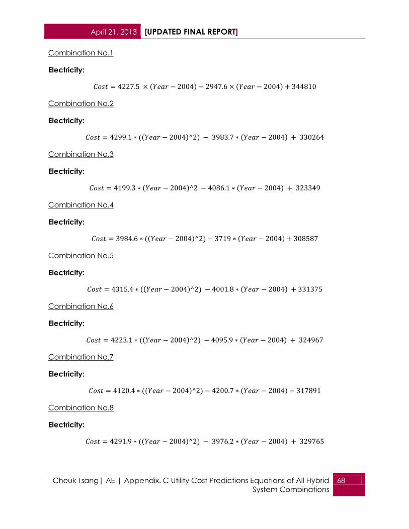
April 21, 2013 [UPDATED FINAL REPORT]
Cheuk Tsang| AE | Appendix. C Utility Cost Predictions Equations of All Hybrid
System Combinations
68
Combination No.1
Electricity:
Combination No.2
Electricity:
Combination No.3
Electricity:
Combination No.4
Electricity:
Combination No.5
Electricity:
Combination No.6
Electricity:
Combination No.7
Electricity:
Combination No.8
Electricity:
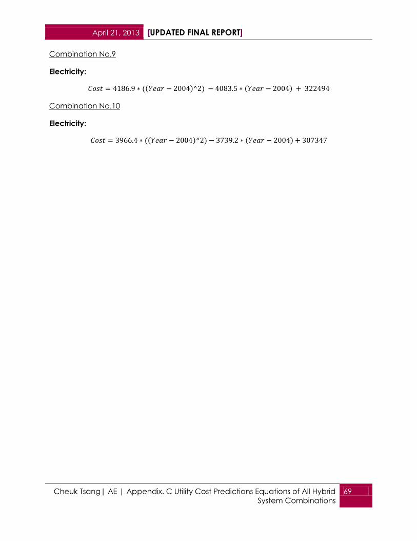
April 21, 2013 [UPDATED FINAL REPORT]
Cheuk Tsang| AE | Appendix. C Utility Cost Predictions Equations of All Hybrid
System Combinations
69
Combination No.9
Electricity:
Combination No.10
Electricity:

April 21, 2013 [UPDATED FINAL REPORT]
Cheuk Tsang| AE | Appendix. D Annual Utility Cost without Inflation Rates of
Hybrid System Combinations
70
Appendix. D Annual Utility Cost without Inflation Rates of Hybrid
System Combinations
Combination
Year Electricity Steam Natural gas Water electricity steam Natural gas Water electricity steam Natural gas water
2015 823913.90 0.00 55882.37655 36659.49 806634.4 150321.162 55882.37655 45009.86511 786517.2 326608.3371 55882.37655 45009.86511
2016 918198.80 0.00 64551.14232 40308.30 901530.0 161798.0237 64551.14232 49489.81725 879015.0 351528.5818 64551.14232 49489.81725
2017 1020938.70 0.00 73219.90809 44202.91 1005023.8 173274.8854 73219.90809 54271.54906 979911.4 376448.8265 73219.90809 54271.54906
2018 1132133.60 0.00 81888.67386 48343.31 1117115.8 184751.7471 81888.67386 59355.06056 1089206.4 401369.0712 81888.67386 59355.06056
2019 1251783.50 0.00 90557.43963 52729.51 1237806.0 196228.6088 90557.43963 64740.35174 1206900.0 426289.3159 90557.43963 64740.35174
2020 1379888.40 0.00 99226.2054 57361.49 1367094.4 207705.4705 99226.2054 70427.42259 1332992.2 451209.5606 99226.2054 70427.42259
2021 1516448.30 0.00 107894.9712 62239.27 1504981.0 219182.3322 107894.9712 76416.27313 1467483.0 476129.8053 107894.9712 76416.27313
2022 1661463.20 0.00 116563.7369 67362.84 1651465.8 230659.1939 116563.7369 82706.90334 1610372.4 501050.05 116563.7369 82706.90334
2023 1814933.10 0.00 125232.5027 72732.21 1806548.8 242136.0556 125232.5027 89299.31324 1761660.4 525970.2947 125232.5027 89299.31324
2024 1976858.00 0.00 133901.2685 78347.37 1970230.0 253612.9173 133901.2685 96193.50281 1921347.0 550890.5394 133901.2685 96193.50281
2025 2147237.90 0.00 142570.0343 84208.31 2142509.4 265089.779 142570.0343 103389.4721 2089432.2 575810.784 142570.0343 103389.4721
2026 2326072.80 0.00 151238.8 90315.06 2323387.0 276566.6408 151238.8 110887.221 2265916.0 600731.0287 151238.8 110887.221
2027 2513362.70 0.00 159907.5658 96667.59 2512862.8 288043.5025 159907.5658 118686.7496 2450798.4 625651.2734 159907.5658 118686.7496
2028 2709107.60 0.00 168576.3316 103265.92 2710936.8 299520.3642 168576.3316 126788.0579 2644079.4 650571.5181 168576.3316 126788.0579
2029 2913307.50 0.00 177245.0973 110110.04 2917609.0 310997.2259 177245.0973 135191.1459 2845759.0 675491.7628 177245.0973 135191.1459
2030 3125962.40 0.00 185913.8631 117199.95 3132879.4 322474.0876 185913.8631 143896.0135 3055837.2 700412.0075 185913.8631 143896.0135
2031 3347072.30 0.00 194582.6289 124535.65 3356748.0 333950.9493 194582.6289 152902.6608 3274314.0 725332.2522 194582.6289 152902.6608
2032 3576637.20 0.00 203251.3946 132117.15 3589214.8 345427.811 203251.3946 162211.0878 3501189.4 750252.4969 203251.3946 162211.0878
2033 3814657.10 0.00 211920.1604 139944.44 3830279.8 356904.6727 211920.1604 171821.2945 3736463.4 775172.7416 211920.1604 171821.2945
2034 4061132.00 0.00 220588.9262 148017.52 4079943.0 368381.5344 220588.9262 181733.2809 3980136.0 800092.9863 220588.9262 181733.2809
2035 4316061.90 0.00 229257.692 156336.39 4338204.4 379858.3961 229257.692 191947.0469 4232207.2 825013.231 229257.692 191947.0469
321
Combination
Year electricity steam Natural gas water electricity steam Natural gas water
2015 786517.2 326608.3371 55882.37655 45009.86511 749814.60 502445.2705 55882.37655 67478.10882
2016 879015.0 351528.5818 64551.14232 49489.81725 837741.40 540722.2334 64551.14232 74194.38529
2017 979911.4 376448.8265 73219.90809 54271.54906 933637.40 578999.1963 73219.90809 81363.08529
2018 1089206.4 401369.0712 81888.67386 59355.06056 1037502.60 617276.1592 81888.67386 88984.20882
2019 1206900.0 426289.3159 90557.43963 64740.35174 1149337.00 655553.1221 90557.43963 97057.75588
2020 1332992.2 451209.5606 99226.2054 70427.42259 1269140.60 693830.085 99226.2054 105583.7265
2021 1467483.0 476129.8053 107894.9712 76416.27313 1396913.40 732107.048 107894.9712 114562.1206
2022 1610372.4 501050.05 116563.7369 82706.90334 1532655.40 770384.0109 116563.7369 123992.9382
2023 1761660.4 525970.2947 125232.5027 89299.31324 1676366.60 808660.9738 125232.5027 133876.1794
2024 1921347.0 550890.5394 133901.2685 96193.50281 1828047.00 846937.9367 133901.2685 144211.8441
2025 2089432.2 575810.784 142570.0343 103389.4721 1987696.60 885214.8996 142570.0343 154999.9324
2026 2265916.0 600731.0287 151238.8 110887.221 2155315.40 923491.8625 151238.8 166240.4441
2027 2450798.4 625651.2734 159907.5658 118686.7496 2330903.40 961768.8254 159907.5658 177933.3794
2028 2644079.4 650571.5181 168576.3316 126788.0579 2514460.60 1000045.788 168576.3316 190078.7382
2029 2845759.0 675491.7628 177245.0973 135191.1459 2705987.00 1038322.751 177245.0973 202676.5206
2030 3055837.2 700412.0075 185913.8631 143896.0135 2905482.60 1076599.714 185913.8631 215726.7265
2031 3274314.0 725332.2522 194582.6289 152902.6608 3112947.40 1114876.677 194582.6289 229229.3559
2032 3501189.4 750252.4969 203251.3946 162211.0878 3328381.40 1153153.64 203251.3946 243184.4088
2033 3736463.4 775172.7416 211920.1604 171821.2945 3551784.60 1191430.603 211920.1604 257591.8853
2034 3980136.0 800092.9863 220588.9262 181733.2809 3783157.00 1229707.566 220588.9262 272451.7853
2035 4232207.2 825013.231 229257.692 191947.0469 4022498.60 1267984.529 229257.692 287764.1088
3 4

April 21, 2013 [UPDATED FINAL REPORT]
Cheuk Tsang| AE | Appendix. D Annual Utility Cost without Inflation Rates of
Hybrid System Combinations
71
Combination
Year electricity steam Natural gas water electricity steam Natural gas water
2015 809518.6 93959.92581 55882.37655 44584.2746 790907.2 203080.5133 55882.37655 44569.59906
2016 904771.0 101138.5141 64551.14232 49021.86658 883942.6 218675.056 64551.14232 49005.73035
2017 1008654.2 108317.1023 73219.90809 53758.38476 985424.2 234269.5987 73219.90809 53740.68944
2018 1121168.2 115495.6906 81888.67386 58793.82914 1095352.0 249864.1414 81888.67386 58774.47634
2019 1242313.0 122674.2788 90557.43963 64128.19973 1213726.0 265458.6841 90557.43963 64107.09104
2020 1372088.6 129852.8671 99226.2054 69761.49652 1340546.2 281053.2269 99226.2054 69738.53356
2021 1510495.0 137031.4554 107894.9712 75693.71952 1475812.6 296647.7696 107894.9712 75668.80388
2022 1657532.2 144210.0436 116563.7369 81924.86872 1619525.2 312242.3123 116563.7369 81897.90201
2023 1813200.2 151388.6319 125232.5027 88454.94412 1771684.0 327836.855 125232.5027 88425.82794
2024 1977499.0 158567.2201 133901.2685 95283.94572 1932289.0 343431.3977 133901.2685 95252.58168
2025 2150428.6 165745.8084 142570.0343 102411.8735 2101340.2 359025.9405 142570.0343 102378.1632
2026 2331989.0 172924.3967 151238.8 109838.7275 2278837.6 374620.4832 151238.8 109802.5726
2027 2522180.2 180102.9849 159907.5658 117564.5078 2464781.2 390215.0259 159907.5658 117525.8098
2028 2721002.2 187281.5732 168576.3316 125589.2142 2659171.0 405809.5686 168576.3316 125547.8747
2029 2928455.0 194460.1614 177245.0973 133912.8468 2862007.0 421404.1114 177245.0973 133868.7675
2030 3144538.6 201638.7497 185913.8631 142535.4056 3073289.2 436998.6541 185913.8631 142488.4881
2031 3369253.0 208817.3379 194582.6289 151456.8906 3293017.6 452593.1968 194582.6289 151407.0365
2032 3602598.2 215995.9262 203251.3946 160677.3019 3521192.2 468187.7395 203251.3946 160624.4127
2033 3844574.2 223174.5145 211920.1604 170196.6393 3757813.0 483782.2822 211920.1604 170140.6167
2034 4095181.0 230353.1027 220588.9262 180014.9029 4002880.0 499376.825 220588.9262 179955.6485
2035 4354418.6 237531.691 229257.692 190132.0928 4256393.2 514971.3677 229257.692 190069.5082
5 6
Combination
Year electricity steam Natural gas water electricity steam Natural gas water
2015 770251.70 264269.8744 55882.37655 62679.20896 805346.7 0 73860.6726 42206.83797
2016 860820.20 284423.1105 64551.14232 68917.8381 900084.2 0 85318.32544 46407.79733
2017 959629.50 304576.3466 73219.90809 75576.71537 1003405.5 0 96775.97828 50891.74278
2018 1066679.60 324729.5826 81888.67386 82655.84078 1115310.6 0 108233.6311 55658.67433
2019 1181970.50 344882.8187 90557.43963 90155.2143 1235799.5 0 119691.284 60708.59198
2020 1305502.20 365036.0548 99226.2054 98074.83596 1364872.2 0 131148.9368 66041.49572
2021 1437274.70 385189.2908 107894.9712 106414.7057 1502528.7 0 142606.5896 71657.38556
2022 1577288.00 405342.5269 116563.7369 115174.8237 1648769.0 0 154064.2425 77556.2615
2023 1725542.10 425495.763 125232.5027 124355.1897 1803593.1 0 165521.8953 83738.12353
2024 1882037.00 445648.9991 133901.2685 133955.8039 1967001.0 0 176979.5482 90202.97166
2025 2046772.70 465802.2351 142570.0343 143976.6662 2138992.7 0 188437.201 96950.80588
2026 2219749.20 485955.4712 151238.8 154417.7766 2319568.2 0 199894.8538 103981.6262
2027 2400966.50 506108.7073 159907.5658 165279.1352 2508727.5 0 211352.5067 111295.4326
2028 2590424.60 526261.9433 168576.3316 176560.7418 2706470.6 0 222810.1595 118892.2251
2029 2788123.50 546415.1794 177245.0973 188262.5967 2912797.5 0 234267.8124 126772.0037
2030 2994063.20 566568.4155 185913.8631 200384.6996 3127708.2 0 245725.4652 134934.7684
2031 3208243.70 586721.6515 194582.6289 212927.0507 3351202.7 0 257183.118 143380.5193
2032 3430665.00 606874.8876 203251.3946 225889.6499 3583281.0 0 268640.7709 152109.2561
2033 3661327.10 627028.1237 211920.1604 239272.4972 3823943.1 0 280098.4237 161120.9791
2034 3900230.00 647181.3597 220588.9262 253075.5926 4073189.0 0 291556.0766 170415.6882
2035 4147373.70 667334.5958 229257.692 267298.9362 4331018.7 0 303013.7294 179993.3834
7 8
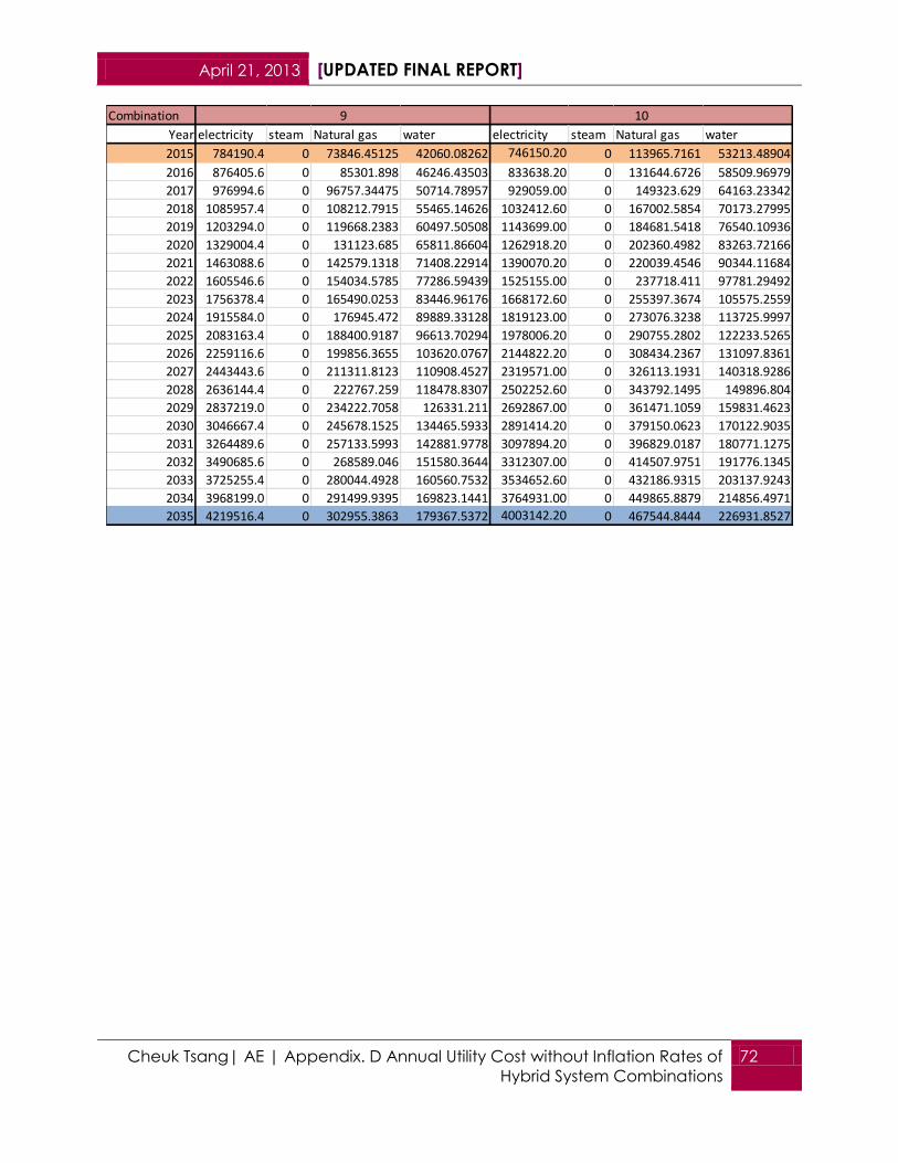
April 21, 2013 [UPDATED FINAL REPORT]
Cheuk Tsang| AE | Appendix. D Annual Utility Cost without Inflation Rates of
Hybrid System Combinations
72
Combination
Year electricity steam Natural gas water electricity steam Natural gas water
2015 784190.4 0 73846.45125 42060.08262 746150.20 0 113965.7161 53213.48904
2016 876405.6 0 85301.898 46246.43503 833638.20 0 131644.6726 58509.96979
2017 976994.6 0 96757.34475 50714.78957 929059.00 0 149323.629 64163.23342
2018 1085957.4 0 108212.7915 55465.14626 1032412.60 0 167002.5854 70173.27995
2019 1203294.0 0 119668.2383 60497.50508 1143699.00 0 184681.5418 76540.10936
2020 1329004.4 0 131123.685 65811.86604 1262918.20 0 202360.4982 83263.72166
2021 1463088.6 0 142579.1318 71408.22914 1390070.20 0 220039.4546 90344.11684
2022 1605546.6 0 154034.5785 77286.59439 1525155.00 0 237718.411 97781.29492
2023 1756378.4 0 165490.0253 83446.96176 1668172.60 0 255397.3674 105575.2559
2024 1915584.0 0 176945.472 89889.33128 1819123.00 0 273076.3238 113725.9997
2025 2083163.4 0 188400.9187 96613.70294 1978006.20 0 290755.2802 122233.5265
2026 2259116.6 0 199856.3655 103620.0767 2144822.20 0 308434.2367 131097.8361
2027 2443443.6 0 211311.8123 110908.4527 2319571.00 0 326113.1931 140318.9286
2028 2636144.4 0 222767.259 118478.8307 2502252.60 0 343792.1495 149896.804
2029 2837219.0 0 234222.7058 126331.211 2692867.00 0 361471.1059 159831.4623
2030 3046667.4 0 245678.1525 134465.5933 2891414.20 0 379150.0623 170122.9035
2031 3264489.6 0 257133.5993 142881.9778 3097894.20 0 396829.0187 180771.1275
2032 3490685.6 0 268589.046 151580.3644 3312307.00 0 414507.9751 191776.1345
2033 3725255.4 0 280044.4928 160560.7532 3534652.60 0 432186.9315 203137.9243
2034 3968199.0 0 291499.9395 169823.1441 3764931.00 0 449865.8879 214856.4971
2035 4219516.4 0 302955.3863 179367.5372 4003142.20 0 467544.8444 226931.8527
9 10

April 21, 2013 [UPDATED FINAL REPORT]
Cheuk Tsang| AE | Appendix. E Interest Rates and Projected furl price indices
Used in Sensitive Analysis
73
Appendix. E Interest Rates and Projected furl price indices Used in
Sensitive Analysis
inflation rate 3%
interest
rate projected fuel price indices
Year SPV Electricity Natural Gas
2012 1 0.99 1.01
2013 0.978 0.98 1.01
2014 0.956 1 1
2015 0.934 1.02 1.01
2016 0.913 1.05 1.05
2017 0.893 1.08 1.09
2018 0.872 1.11 1.13
2019 0.853 1.15 1.18
2020 0.834 1.2 1.23
2021 0.815 1.25 1.28
2022 0.797 1.3 1.34
2023 0.779 1.34 1.39
2024 0.761 1.38 1.45
2025 0.744 1.43 1.52
2026 0.727 1.47 1.58
2027 0.711 1.51 1.64
2028 0.695 1.55 1.71
2029 0.679 1.59 1.78
2030 0.664 1.64 1.85
2031 0.649 1.69 1.92
2032 0.635 1.74 1.99
2033 0.62 1.8 2.07
2034 0.606 1.87 2.14
2035 0.593 1.93 2.22
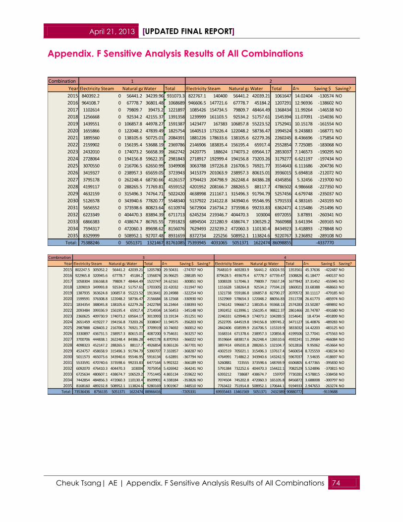
April 21, 2013 [UPDATED FINAL REPORT]
Cheuk Tsang| AE | Appendix. F Sensitive Analysis Results of All Combinations 74
Appendix. F Sensitive Analysis Results of All Combinations
Combination
Year Electricity Steam Natural gasWater Total Electricity Steam Natural gasWater Total ∆ % Saving $ Saving?
2015 840392.2 0 56441.2 34239.96 931073.3 822767.1 140400 56441.2 42039.21 1061647 14.02404 -130574 NO
2016 964108.7 0 67778.7 36801.48 1068689 946606.5 147721.6 67778.7 45184.2 1207291 12.96936 -138602 NO
2017 1102614 0 79809.7 39473.2 1221897 1085426 154734.5 79809.7 48464.49 1368434 11.99264 -146538 NO
2018 1256668 0 92534.2 42155.37 1391358 1239999 161103.5 92534.2 51757.61 1545394 11.07091 -154036 NO
2019 1439551 0 106857.8 44978.27 1591387 1423477 167383 106857.8 55223.52 1752941 10.15178 -161554 NO
2020 1655866 0 122048.2 47839.49 1825754 1640513 173226.4 122048.2 58736.47 1994524 9.243883 -168771 NO
2021 1895560 0 138105.6 50725.01 2084391 1881226 178633.6 138105.6 62279.26 2260245 8.436696 -175854 NO
2022 2159902 0 156195.4 53688.19 2369786 2146906 183835.4 156195.4 65917.4 2552854 7.725085 -183068 NO
2023 2432010 0 174073.2 56658.39 2662742 2420775 188624 174073.2 69564.17 2853037 7.146573 -190295 NO
2024 2728064 0 194156.8 59622.35 2981843 2718917 192999.4 194156.8 73203.26 3179277 6.621197 -197434 NO
2025 3070550 0 216706.5 62650.99 3349908 3063788 197226.8 216706.5 76921.77 3554643 6.111686 -204736 NO
2026 3419327 0 238957.3 65659.05 3723943 3415379 201063.9 238957.3 80615.01 3936015 5.694818 -212072 NO
2027 3795178 0 262248.4 68730.66 4126157 3794423 204798.9 262248.4 84386.28 4345856 5.32456 -219700 NO
2028 4199117 0 288265.5 71769.81 4559152 4201952 208166.7 288265.5 88117.7 4786502 4.986668 -227350 NO
2029 4632159 0 315496.3 74764.71 5022420 4638998 211167.1 315496.3 91794.79 5257456 4.679748 -235037 NO
2030 5126578 0 343940.6 77820.77 5548340 5137922 214122.8 343940.6 95546.95 5791533 4.383165 -243193 NO
2031 5656552 0 373598.6 80823.64 6110974 5672904 216734.2 373598.6 99233.83 6362471 4.115486 -251496 NO
2032 6223349 0 404470.3 83894.39 6711713 6245234 219346.7 404470.3 103004 6972055 3.87891 -260341 NO
2033 6866383 0 438674.7 86765.55 7391823 6894504 221280.9 438674.7 106529.2 7660988 3.641394 -269165 NO
2034 7594317 0 472060.3 89698.62 8156076 7629493 223239.2 472060.3 110130.4 8434923 3.418893 -278848 NO
2035 8329999 0 508952.1 92707.48 8931659 8372734 225256 508952.1 113824.6 9220767 3.236892 -289108 NO
Total: 75388246 0 5051371 1321467 81761085 75393945 4031065 5051371 1622474 86098855 -4337770
1 2
Combination
Year Electricity Steam Natural gasWater Total ∆ % Saving $ Saving? Electricity Steam Natural gasWater Total ∆ % Saving $ Saving?
2015 802247.5 305052.2 56441.2 42039.21 1205780 29.50431 -274707 NO 764810.9 469283.9 56441.2 63024.55 1353561 45.37636 -422487 NO
2016 922965.8 320945.6 67778.7 45184.2 1356874 26.96625 -288185 NO 879628.5 493679.4 67778.7 67739.47 1508826 41.18477 -440137 NO
2017 1058304 336168.8 79809.7 48464.49 1522747 24.62161 -300851 NO 1008328 517046.3 79809.7 72657.24 1677842 37.31452 -455945 NO
2018 1209019 349993.8 92534.2 51757.61 1703305 22.42032 -311947 NO 1151628 538264.8 92534.2 77594.23 1860021 33.68388 -468663 NO
2019 1387935 363624.8 106857.8 55223.52 1913641 20.24988 -322254 NO 1321738 559186.8 106857.8 82790.27 2070572 30.11117 -479185 NO
2020 1599591 376308.8 122048.2 58736.47 2156684 18.12568 -330930 NO 1522969 578654.3 122048.2 88056.83 2311728 26.61773 -485974 NO
2021 1834354 388045.8 138105.6 62279.26 2422784 16.23464 -338393 NO 1746142 596667.2 138105.6 93368.13 2574283 23.50287 -489892 NO
2022 2093484 399336.9 156195.4 65917.4 2714934 14.56453 -345148 NO 1992452 613996.1 156195.4 98822.37 2861466 20.74787 -491680 NO
2023 2360625 409730.9 174073.2 69564.17 3013993 13.19134 -351251 NO 2246331 629946.9 174073.2 104289.5 3154641 18.4734 -491899 NO
2024 2651459 419227.7 194156.8 73203.26 3338047 11.94575 -356203 NO 2522705 644519.8 194156.8 109745.2 3471127 16.40876 -489283 NO
2025 2987888 428403.2 216706.5 76921.77 3709919 10.74692 -360012 NO 2842406 658599.9 216706.5 115319.9 3833032 14.42203 -483125 NO
2026 3330897 436731.5 238957.3 80615.01 4087200 9.754631 -363257 NO 3168314 671378.6 238957.3 120856.8 4199506 12.77041 -475563 NO
2027 3700706 444838.1 262248.4 84386.28 4492178 8.870763 -366022 NO 3519664 683817.6 262248.4 126510.6 4592241 11.29584 -466084 NO
2028 4098323 452147.2 288265.5 88117.7 4926854 8.065126 -367701 NO 3897414 695031.8 288265.5 132104.7 5012816 9.95062 -453664 NO
2029 4524757 458658.9 315496.3 91794.79 5390707 7.332857 -368287 NO 4302519 705021.1 315496.3 137617.4 5460654 8.725559 -438234 NO
2030 5011573 465073.6 343940.6 95546.95 5916134 6.62891 -367794 NO 4764991 714862.2 343940.6 143242.5 5967037 7.54635 -418697 NO
2031 5533591 470740.6 373598.6 99233.83 6477164 5.992322 -366189 NO 5260881 723555 373598.6 148769.9 6506805 6.477365 -395830 NO
2032 6092070 476410.3 404470.3 103004 7075954 5.426942 -364241 NO 5791384 732252.6 404470.3 154422.1 7082529 5.524896 -370815 NO
2033 6725634 480607.1 438674.7 106529.2 7751445 4.865134 -359622 NO 6393212 738687 438674.7 159707 7730281 4.578815 -338458 NO
2034 7442854 484856.3 472060.3 110130.4 8509901 4.338184 -353826 NO 7074504 745202.8 472060.3 165105.8 8456872 3.688008 -300797 NO
2035 8168160 489232.8 508952.1 113824.6 9280169 3.901967 -348510 NO 7763422 751914.8 508952.1 170644.1 9194933 2.947653 -263274 NO
Total: 73536436 8756135 5051371 1622474 88966416 -7205331 69935443 13461569 5051371 2432389 90880772 -9119688
43

April 21, 2013 [UPDATED FINAL REPORT]
Cheuk Tsang| AE | Appendix. F Sensitive Analysis Results of All Combinations 75
Combination
Year Electricity Steam Natural gasWater Total ∆ % Saving $ Saving? Electricity Steam Natural gasWater Total ∆ % Saving $ Saving?
2015 825709 87758.57 56441.2 41641.71 1011550 8.643478 -80477.1 NO 806725.3 189677.2 56441.2 41628.01 1094472 17.54947 -163398 NO
2016 950009.6 92339.46 67778.7 44756.96 1154885 8.065561 -86195.8 NO 928139.7 199650.3 67778.7 44742.23 1240311 16.05912 -171622 NO
2017 1089347 96727.17 79809.7 48006.24 1313890 7.528701 -91992.9 NO 1064258 209202.8 79809.7 47990.44 1401261 14.67917 -179364 NO
2018 1244497 100712.2 92534.2 51268.22 1489011 7.018575 -97653.5 NO 1215841 217881.5 92534.2 51251.34 1577508 13.37901 -186150 NO
2019 1428660 104641.2 106857.8 54701.35 1694860 6.502074 -103473 NO 1395785 226436.3 106857.8 54683.35 1783762 12.08852 -192375 NO
2020 1646506 108297.3 122048.2 58181.09 1935033 5.985425 -109279 NO 1608655 234398.4 122048.2 58161.94 2023264 10.81801 -197510 NO
2021 1888119 111680.6 138105.6 61690.38 2199595 5.527005 -115204 NO 1844766 241767.9 138105.6 61670.08 2286309 9.687164 -201918 NO
2022 2154792 114935.4 156195.4 65294.12 2491217 5.124136 -121431 NO 2105383 248857.1 156195.4 65272.63 2575708 8.689484 -205922 NO
2023 2429688 117931.7 174073.2 68906.4 2790600 4.80173 -127858 NO 2374057 255384.9 174073.2 68883.72 2872398 7.873705 -209656 NO
2024 2728949 120669.7 194156.8 72511.08 3116286 4.50872 -134443 NO 2666559 261351.3 194156.8 72487.21 3194554 7.133539 -212711 NO
2025 3075113 123314.9 216706.5 76194.43 3491329 4.22164 -141421 NO 3004916 267115.3 216706.5 76169.35 3564908 6.418086 -215000 NO
2026 3428024 125716 238957.3 79852.75 3872550 3.99057 -148607 NO 3349891 272349.1 238957.3 79826.47 3941024 5.829325 -217081 NO
2027 3808492 128053.2 262248.4 83588.37 4282382 3.78622 -156225 NO 3721820 277442.9 262248.4 83560.85 4345072 5.305543 -218915 NO
2028 4217553 130160.7 288265.5 87284.5 4723264 3.599617 -164112 NO 4121715 282037.7 288265.5 87255.77 4779274 4.828132 -220122 NO
2029 4656243 132038.4 315496.3 90926.82 5194705 3.43032 -172285 NO 4550591 286133.4 315496.3 90896.89 5243118 4.394252 -220698 NO
2030 5157043 133888.1 343940.6 94643.51 5729516 3.265406 -181176 NO 5040194 290167.1 343940.6 94612.36 5768914 3.975507 -220575 NO
2031 5694038 135522.5 373598.6 98295.52 6301454 3.117011 -190480 NO 5565200 293733 373598.6 98263.17 6330795 3.597136 -219820 NO
2032 6268521 137157.4 404470.3 102030.1 6912179 2.986797 -200465 NO 6126874 297299.2 404470.3 101996.5 6930640 3.261865 -218927 NO
2033 6920234 138368.2 438674.7 105521.9 7602798 2.854172 -210975 NO 6764063 299945 438674.7 105487.2 7608170 2.926846 -216347 NO
2034 7657988 139594 472060.3 109089 8378732 2.729941 -222656 NO 7485386 302622.4 472060.3 109053.1 8369121 2.612109 -213046 NO
2035 8404028 140856.3 508952.1 112748.3 9166585 2.630257 -234926 NO 8214839 305378 508952.1 112711.2 9141880 2.353663 -210221 NO
Total: 75673553 2520363 5051371 1607133 84852420 -3091335 73955658 5458831 5051371 1606604 86072464 -4311379
65
Combination
Year Electricity Steam Natural gasWater Total ∆ % Saving $ Saving? Electricity Steam Natural gasWater Total ∆ % Saving $ Saving?
2015 785656.7 246828.1 56441.2 58542.38 1147468 23.24146 -163398 NO 821453.6 0 74599.28 39421.19 935474.1 0.472655 -4400.76 No
2016 903861.2 259678.3 67778.7 62921.99 1294240 21.10542 -171622 NO 945088.4 0 89584.24 42370.32 1077043 0.78171 -8354.05 No
2017 1036400 271986.7 79809.7 67490.01 1455686 19.13333 -179364 NO 1083678 0 105485.8 45446.33 1234610 1.040463 -12713.4 No
2018 1184014 283164.2 92534.2 72075.89 1631789 17.2803 -186150 NO 1237995 0 122304 48534.36 1408833 1.255986 -17475.3 No
2019 1359266 294185 106857.8 76902.4 1837211 15.44717 -192375 NO 1421169 0 141235.7 51784.43 1614190 1.432869 -22802.5 No
2020 1566603 304440.1 122048.2 81794.41 2074885 13.64541 -197510 NO 1637847 0 161313.2 55078.61 1854238 1.560158 -28484.6 No
2021 1796593 313929.3 138105.6 86727.99 2335356 12.04022 -201918 NO 1878161 0 182536.4 58400.77 2119098 1.665097 -34707.1 No
2022 2050474 323058 156195.4 91794.33 2621522 10.62275 -205922 NO 2143400 0 206446.1 61812.34 2411658 1.766926 -41872.4 No
2023 2312226 331461.2 174073.2 96872.69 2914633 9.459856 -209656 NO 2416815 0 230075.4 65232 2712122 1.854489 -49380.3 No
2024 2597211 339138.9 194156.8 101940.4 3232447 8.40433 -212711 NO 2714461 0 256620.3 68644.46 3039726 1.941181 -57883 No
2025 2926885 346556.9 216706.5 107118.6 3597267 7.384063 -215000 NO 3058760 0 286424.5 72131.4 3417316 2.012231 -67407.9 No
2026 3263031 353289.6 238957.3 112261.7 3967540 6.541362 -217081 NO 3409765 0 315833.9 75594.64 3801194 2.074425 -77250.4 No
2027 3625459 359843.3 262248.4 117513.5 4365065 5.790081 -218915 NO 3788179 0 346618.1 79131.05 4213928 2.127184 -87770.9 No
2028 4015158 365752.1 288265.5 122709.7 4791885 5.10475 -220122 NO 4195029 0 381005.4 82630.1 4658665 2.182704 -99512.8 No
2029 4433116 371015.9 315496.3 127830.3 5247459 4.480687 -220698 NO 4631348 0 416996.7 86078.19 5134423 2.230061 -112003 No
2030 4910264 376201.4 343940.6 133055.4 5763461 3.877221 -220575 NO 5129441 0 454592.1 89596.69 5673630 2.258162 -125290 No
2031 5421932 380782.4 373598.6 138189.7 6314503 3.330533 -219820 NO 5663533 0 493791.6 93053.96 6250378 2.281201 -139404 No
2032 5969357 385365.6 404470.3 143439.9 6902633 2.844571 -218927 NO 6234909 0 534595.1 96589.38 6866093 2.300159 -154380 No
2033 6590389 388757.4 438674.7 148348.9 7566170 2.358645 -216347 NO 6883098 0 579803.7 99895.01 7562796 2.313005 -170973 No
2034 7293430 392191.9 472060.3 153363.8 8311046 1.90006 -213046 NO 7616863 0 623930 103271.9 8344065 2.304902 -187990 No
2035 8004431 395729.4 508952.1 158508.3 9067621 1.522248 -210221 NO 8358866 0 672690.5 106736.1 9138293 2.313497 -206634 No
Total: 72045759 7083356 5051371 2259402 86439888 -4311379 75269858 0 6676482 1521433 83467774 -1706689
87

April 21, 2013 [UPDATED FINAL REPORT]
Cheuk Tsang| AE | Appendix. F Sensitive Analysis Results of All Combinations 76
Combination
Year Electricity Steam Natural gasWater Total ∆ % Saving $ Saving? Electricity Steam Natural gasWater Total ∆ % Saving $ Saving?
2015 799874.2 0 74584.92 39284.12 913743.2 -1.8613 17330.1 YES 761073.2 0 115105.4 49701.4 925880 -0.55778 5193.362 YES
2016 920225.9 0 89566.99 42223 1052016 -1.56014 16673.05 YES 875320.1 0 138226.9 53419.6 1066967 -0.16116 1722.301 YES
2017 1055154 0 105465.5 45288.31 1205908 -1.30852 15988.71 YES 1003384 0 162762.8 57297.77 1223444 0.126651 -1547.55 NO
2018 1205413 0 122280.5 48365.61 1376059 -1.09958 15299.09 YES 1145978 0 188712.9 61191.1 1395882 0.32516 -4524.14 NO
2019 1383788 0 141208.5 51604.37 1576601 -0.92913 14786.08 YES 1315254 0 217924.2 65288.71 1598467 0.444877 -7079.71 NO
2020 1594805 0 161282.1 54887.1 1810975 -0.80949 14779.29 YES 1515502 0 248903.4 69441.94 1833847 0.443291 -8093.4 NO
2021 1828861 0 182501.3 58197.71 2069560 -0.71154 14831.2 YES 1737588 0 281650.5 73630.46 2092869 0.406726 -8477.76 NO
2022 2087211 0 206406.3 61597.42 2355214 -0.61488 14571.42 YES 1982702 0 318542.7 77931.69 2379176 0.396243 -9390.11 NO
2023 2353547 0 230031.1 65005.18 2648583 -0.53173 14158.55 YES 2235351 0 355002.3 82243.12 2672597 0.370101 -9854.83 NO
2024 2643506 0 256570.9 68405.78 2968483 -0.44806 13360.59 YES 2510390 0 395960.7 86545.49 2992896 0.370666 -11052.7 NO
2025 2978924 0 286369.4 71880.59 3337174 -0.38013 12733.98 YES 2828549 0 441948 90941.74 3361439 0.344218 -11531 NO
2026 3320901 0 315773.1 75331.8 3712006 -0.32055 11937.11 YES 3152889 0 487326.1 95308.13 3735523 0.310947 -11579.5 NO
2027 3689600 0 346551.4 78855.91 4115007 -0.27022 11149.62 YES 3502552 0 534825.6 99766.76 4137145 0.266298 -10987.9 NO
2028 4086024 0 380932 82342.79 4549299 -0.21613 9853.499 YES 3878492 0 587884.6 104178.3 4570554 0.250096 -11402.3 NO
2029 4511178 0 416916.4 85778.89 5013874 -0.17016 8546.395 YES 4281659 0 643418.6 108525.6 5033603 0.222657 -11182.7 NO
2030 4996535 0 454504.6 89285.15 5540324 -0.14447 8015.476 YES 4741919 0 701427.6 112961.6 5556309 0.143624 -7968.76 NO
2031 5516987 0 493696.5 92730.4 6103414 -0.12371 7560.135 YES 5235441 0 761911.7 117320.5 6114673 0.060529 -3698.9 NO
2032 6073793 0 534492.2 96253.53 6704539 -0.1069 7174.716 YES 5763414 0 824870.9 121777.8 6710063 -0.02459 1650.497 YES
2033 6705460 0 579692.1 99547.67 7384699 -0.09637 7123.577 YES 6362375 0 894626.9 125945.5 7382947 -0.12008 8875.923 YES
2034 7420532 0 623809.9 102912.8 8147255 -0.10815 8820.934 YES 7040421 0 962713 130203 8133337 -0.2788 22738.75 YES
2035 8143667 0 672561 106364.9 8922593 -0.10151 9066.466 YES 7726064 0 1037950 134570.6 8898585 -0.37031 33074.44 YES
Total: 73315985 6675197 81507325 253760 69596316 10301694 1918191 81816201 -55115.9
109
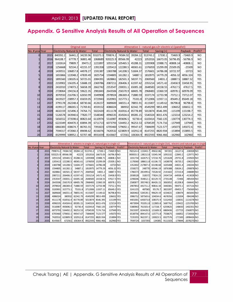
April 21, 2013 [UPDATED FINAL REPORT]
Cheuk Tsang| AE | Appendix. G Sensitive Analysis Results of All Operation of
Sequences
77
Appendix. G Sensitive Analysis Results of All Operation of Sequences
No. # year Year Electricity Natural GasWater Total Electricity Natural GasWater Total Saving (+) Payback Profit?
0 2015 840392.2 56441.2 34239.96 931073.3 799874.2 74584.92 39284.12 913743.2 17330.1 73469.9 -73469.9 NO
1 2016 964108.7 67778.7 36801.48 1068689 920225.9 89566.99 42223 1052016 16673.05 56796.85 -56796.9 NO
2 2017 1102614 79809.7 39473.2 1221897 1055154 105465.5 45288.31 1205908 15988.71 40808.14 -40808.1 NO
3 2018 1256668 92534.2 42155.37 1391358 1205413 122280.5 48365.61 1376059 15299.09 25509.05 -25509 NO
4 2019 1439551 106857.8 44978.27 1591387 1383788 141208.5 51604.37 1576601 14786.08 10722.97 -10723 NO
5 2020 1655866 122048.2 47839.49 1825754 1594805 161282.1 54887.1 1810975 14779.29 -4056.32 4056.324 YES
6 2021 1895560 138105.6 50725.01 2084391 1828861 182501.3 58197.71 2069560 14831.2 -18887.5 18887.52 YES
7 2022 2159902 156195.4 53688.19 2369786 2087211 206406.3 61597.42 2355214 14571.42 -33458.9 33458.95 YES
8 2023 2432010 174073.2 56658.39 2662742 2353547 230031.1 65005.18 2648583 14158.55 -47617.5 47617.5 YES
9 2024 2728064 194156.8 59622.35 2981843 2643506 256570.9 68405.78 2968483 13360.59 -60978.1 60978.09 YES
10 2025 3070550 216706.5 62650.99 3349908 2978924 286369.4 71880.59 3337174 12733.98 -73712.1 73712.07 YES
11 2026 3419327 238957.3 65659.05 3723943 3320901 315773.1 75331.8 3712006 11937.11 -85649.2 85649.18 YES
12 2027 3795178 262248.4 68730.66 4126157 3689600 346551.4 78855.91 4115007 11149.62 -96798.8 96798.8 YES
13 2028 4199117 288265.5 71769.81 4559152 4086024 380932 82342.79 4549299 9853.499 -106652 106652.3 YES
14 2029 4632159 315496.3 74764.71 5022420 4511178 416916.4 85778.89 5013874 8546.395 -115199 115198.7 YES
15 2030 5126578 343940.6 77820.77 5548340 4996535 454504.6 89285.15 5540324 8015.476 -123214 123214.2 YES
16 2031 5656552 373598.6 80823.64 6110974 5516987 493696.5 92730.4 6103414 7560.135 -130774 130774.3 YES
17 2032 6223349 404470.3 83894.39 6711713 6073793 534492.2 96253.53 6704539 7174.716 -137949 137949 YES
18 2033 6866383 438674.7 86765.55 7391823 6705460 579692.1 99547.67 7384699 7123.577 -145073 145072.6 YES
19 2034 7594317 472060.3 89698.62 8156076 7420532 623809.9 102912.8 8147255 8820.934 -153894 153893.5 YES
20 2035 8329999 508952.1 92707.48 8931659 8143667 672561 106364.9 8922593 9066.466 -162960 162960 YES
Original cost Altnerative 1 - natural gas x2+ electric x1 (parallel)
No. # year Year Electricity Natural GasWater Total Saving (+) Payback Profit? Electricity Natural GasWater Total Saving (+) Payback Profit?
0 2015 799874.2 74584.92 39284.12 913743.2 17330.1 -73469.9 NO 782524.4 115043.7 49632.86 947201 -16127.6 -106928 NO
1 2016 920225.9 89566.99 42223 1052016 16673.05 -56796.9 NO 900033.3 138152.8 53345.94 1091532 -22843.2 -129771 NO
2 2017 1055154 105465.5 45288.31 1205908 15988.71 -40808.1 NO 1031734 162675.5 57218.76 1251628 -29731.8 -159503 NO
3 2018 1205413 122280.5 48365.61 1376059 15299.09 -25509.1 NO 1178360 188611.8 61106.72 1428078 -36720.2 -196223 NO
4 2019 1383788 141208.5 51604.37 1576601 14786.08 -10723 NO 1352402 217807.4 65198.68 1635408 -44021.4 -240244 NO
5 2020 1594805 161282.1 54887.1 1810975 14779.29 4056.32 YES 1558272 248770 69346.19 1876388 -50634.2 -290878 NO
6 2021 1828861 182501.3 58197.71 2069560 14831.2 18887.5 YES 1786573 281499.6 73528.92 2141602 -57210.8 -348089 NO
7 2022 2087211 206406.3 61597.42 2355214 14571.42 33458.9 YES 2038528 318372 77824.23 2434724 -64938.4 -413028 NO
8 2023 2353547 230031.1 65005.18 2648583 14158.55 47617.5 YES 2298206 354812.1 82129.72 2735148 -72406 -485434 NO
9 2024 2643506 256570.9 68405.78 2968483 13360.59 60978.1 YES 2580877 395748.5 86426.15 3063052 -81208.8 -566642 NO
10 2025 2978924 286369.4 71880.59 3337174 12733.98 73712.1 YES 2907853 441711.2 90816.34 3440381 -90473.1 -657116 NO
11 2026 3320901 315773.1 75331.8 3712006 11937.11 85649.2 YES 3241155 487065 95176.7 3823397 -99453.7 -756569 NO
12 2027 3689600 346551.4 78855.91 4115007 11149.62 96798.8 YES 3600463 534539.1 99629.19 4234631 -108474 -865043 NO
13 2028 4086024 380932 82342.79 4549299 9853.499 106652 YES 3986752 587569.6 104034.6 4678356 -119204 -984248 NO
14 2029 4511178 416916.4 85778.89 5013874 8546.395 115199 YES 4401001 643073.8 108375.9 5152450 -130031 -1114278 NO
15 2030 4996535 454504.6 89285.15 5540324 8015.476 123214 YES 4873904 701051.8 112805.8 5687762 -139422 -1253700 NO
16 2031 5516987 493696.5 92730.4 6103414 7560.135 130774 YES 5380963 761503.4 117158.7 6259625 -148650 -1402351 NO
17 2032 6073793 534492.2 96253.53 6704539 7174.716 137949 YES 5923397 824428.9 121609.9 6869436 -157723 -1560073 NO
18 2033 6705460 579692.1 99547.67 7384699 7123.577 145073 YES 6538756 894147.6 125771.8 7558675 -166852 -1726926 NO
19 2034 7420532 623809.9 102912.8 8147255 8820.934 153894 YES 7235355 962197.1 130023.5 8327576 -171500 -1898426 NO
20 2035 8143667 672561 106364.9 8922593 9066.466 162960 YES 7939724 1037393 134385 9111503 -179844 -2078270 NO
Altnerative 3 - natural gas in single (1st), electric and natural gas in singleAltnerative 2 - electric in single x1, natural gas in single x2

April 21, 2013 [UPDATED FINAL REPORT]
Cheuk Tsang| AE | Appendix. G Sensitive Analysis Results of All Operation of
Sequences
78
No. # year Year Electricity Natural GasWater Total Saving (+) Payback Profit? Electricity Natural GasWater Total Saving (+) Payback Profit?
0 2015 812369.9 82175.64 47001.13 941546.7 -10473.4 -101273 NO 781249.2 115635.1 49838.47 946722.8 -15649.5 -106449 NO
1 2016 934713.6 98682.48 50517.32 1083913 -15224.5 -116498 NO 898565.4 138863.1 53566.93 1090995 -22306.5 -128756 NO
2 2017 1071887 116199 54184.79 1242271 -20374.1 -136872 NO 1030052 163511.9 57455.79 1251020 -29123.1 -157879 NO
3 2018 1224657 134725.3 57866.6 1417249 -25891 -162763 NO 1176441 189581.5 61359.86 1427382 -36024.5 -193904 NO
4 2019 1406017 155579.7 61741.59 1623338 -31951.3 -194714 NO 1350205 218927.2 65468.77 1634601 -43213.5 -237117 NO
5 2020 1620570 177696.3 65669.17 1863935 -38181.2 -232895 NO 1555746 250049 69633.46 1875428 -49674.1 -286791 NO
6 2021 1858560 201075 69630.12 2129265 -44874 -277769 NO 1783685 282946.8 73833.52 2140465 -56073.8 -342865 NO
7 2022 2121266 227412.9 73697.68 2422377 -52591.2 -330361 NO 2035241 320008.7 78146.62 2433396 -63610.6 -406476 NO
8 2023 2392116 253442.1 77774.87 2723333 -60590.9 -390951 NO 2294511 356636.2 82469.94 2733617 -70875.4 -477351 NO
9 2024 2686999 282682.9 81843.48 3051526 -69682.5 -460634 NO 2576740 397783 86784.17 3061307 -79464.1 -556815 NO
10 2025 3028115 315514 86000.89 3429630 -79722.5 -540357 NO 2903205 443982.1 91192.55 3438380 -88472.4 -645288 NO
11 2026 3375925 347910.2 90130.05 3813965 -90021.6 -630378 NO 3235990 489569 95570.97 3821130 -97186.4 -742474 NO
12 2027 3750921 381820.9 94346.45 4227089 -100932 -731310 NO 3594741 537287.1 100041.9 4232070 -105913 -848387 NO
13 2028 4154128 419700.6 98518.29 4672347 -113195 -844505 NO 3980434 590590.3 104465.6 4675490 -116338 -964725 NO
14 2029 4586567 459347.2 102629.4 5148544 -126124 -970629 NO 4394045 646379.8 108824.9 5149249 -126829 -1091554 NO
15 2030 5080239 500760.8 106824.4 5687824 -139484 -1110113 NO 4866220 704655.9 113273.1 5684149 -135810 -1227364 NO
16 2031 5609620 543941.4 110946.5 6264508 -153534 -1263647 NO 5372501 765418.3 117644 6255563 -144589 -1371952 NO
17 2032 6175990 588889 115161.7 6880040 -168327 -1431974 NO 5914105 828667.3 122113.7 6864886 -153173 -1525125 NO
18 2033 6818506 638689 119102.9 7576298 -184475 -1616449 NO 6528522 898744.4 126292.9 7553559 -161736 -1686861 NO
19 2034 7545863 687296.8 123129.1 8356289 -200213 -1816662 NO 7224057 967143.8 130562.1 8321763 -165687 -1852548 NO
20 2035 8281447 741009.4 127259.4 9149716 -218057 -2034719 NO 7927353 1042727 134941.7 9105021 -173362 -2025910 NO
Altnerative 5 - natural gas x1 in sidcar, others in singleAltnerative 4 - natural gas x2 in single + electric x1 in sidecar
No. # year Year Electricity Natural GasWater Total Saving (+) Payback Profit? Electricity Natural GasWater Total Saving (+) Payback Profit?
0 2015 799874.2 74584.92 39284.12 913743.2 17330.1 -73469.9 NO 782524.4 115036.1 49632.86 947193.4 -16120 -106920 NO
1 2016 920225.9 89566.99 42223 1052016 16673.05 -56796.9 NO 900033.3 138143.7 53345.94 1091523 -22834.1 -129754 NO
2 2017 1055154 105465.5 45288.31 1205908 15988.71 -40808.1 NO 1031734 162664.8 57218.76 1251618 -29721 -159475 NO
3 2018 1205413 122280.5 48365.61 1376059 15299.09 -25509 NO 1178360 188599.3 61106.72 1428066 -36707.8 -196183 NO
4 2019 1383788 141208.5 51604.37 1576601 14786.08 -10723 NO 1352402 217793 65198.68 1635394 -44007 -240190 NO
5 2020 1594805 161282.1 54887.1 1810975 14779.29 4056.324 YES 1558272 248753.6 69346.19 1876372 -50617.7 -290808 NO
6 2021 1828861 182501.3 58197.71 2069560 14831.2 18887.52 YES 1786573 281481 73528.92 2141583 -57192.2 -348000 NO
7 2022 2087211 206406.3 61597.42 2355214 14571.42 33458.95 YES 2038528 318350.9 77824.23 2434703 -64917.3 -412917 NO
8 2023 2353547 230031.1 65005.18 2648583 14158.55 47617.5 YES 2298206 354788.7 82129.72 2735125 -72382.6 -485300 NO
9 2024 2643506 256570.9 68405.78 2968483 13360.59 60978.09 YES 2580877 395722.3 86426.15 3063026 -81182.6 -566482 NO
10 2025 2978924 286369.4 71880.59 3337174 12733.98 73712.07 YES 2907853 441682 90816.34 3440352 -90444 -656926 NO
11 2026 3320901 315773.1 75331.8 3712006 11937.11 85649.18 YES 3241155 487032.8 95176.7 3823365 -99421.5 -756348 NO
12 2027 3689600 346551.4 78855.91 4115007 11149.62 96798.8 YES 3600463 534503.7 99629.19 4234596 -108439 -864787 NO
13 2028 4086024 380932 82342.79 4549299 9853.499 106652.3 YES 3986752 587530.7 104034.6 4678318 -119165 -983952 NO
14 2029 4511178 416916.4 85778.89 5013874 8546.395 115198.7 YES 4401001 643031.3 108375.9 5152408 -129988 -1113940 NO
15 2030 4996535 454504.6 89285.15 5540324 8015.476 123214.2 YES 4873904 701005.4 112805.8 5687715 -139376 -1253316 NO
16 2031 5516987 493696.5 92730.4 6103414 7560.135 130774.3 YES 5380963 761453.1 117158.7 6259575 -148600 -1401916 NO
17 2032 6073793 534492.2 96253.53 6704539 7174.716 137949 YES 5923397 824374.4 121609.9 6869382 -157668 -1559584 NO
18 2033 6705460 579692.1 99547.67 7384699 7123.577 145072.6 YES 6538756 894088.5 125771.8 7558616 -166793 -1726377 NO
19 2034 7420532 623809.9 102912.8 8147255 8820.934 153893.5 YES 7235355 962133.5 130023.5 8327512 -171437 -1897814 NO
20 2035 8143667 672561 106364.9 8922593 9066.466 162960 YES 7939724 1037325 134385 9111434 -179775 -2077589 NO
Altnerative 6 - decoupling, electric (1st) Altnerative 7 - decoupling, natural gas (1st)

April 21, 2013 [UPDATED FINAL REPORT]
Cheuk Tsang| AE | Appendix. H Ventilation Distribution of Supplying Air to
Galleries and Offices
79
Appendix. H Ventilation Distribution of Supplying Air to Galleries and
Offices
Ventilation System on Cellar Level
Ventilation System on 9th floor
Supply to Level 7 Level 6 Level 6 Level 5 Level 5 Level 4 Level 4 Level 3 Level 3 Level 1 Total
Duct size 54 x 16 54 x 16 42 x 16 60 x 20 72 x 16 30 x 18 36 x 16 72 x 12 30 x 18 24 x 12
Airflow rate (cfm)9040 6760 5760 12080 12400 5600 7155 6900 3680 1900 92815
Cellar level
Supply to
Duct size 36 x 18 20 x 12 20 x 16
Airflow rate (cfm)6760 1120 4120
9th level
Level 8
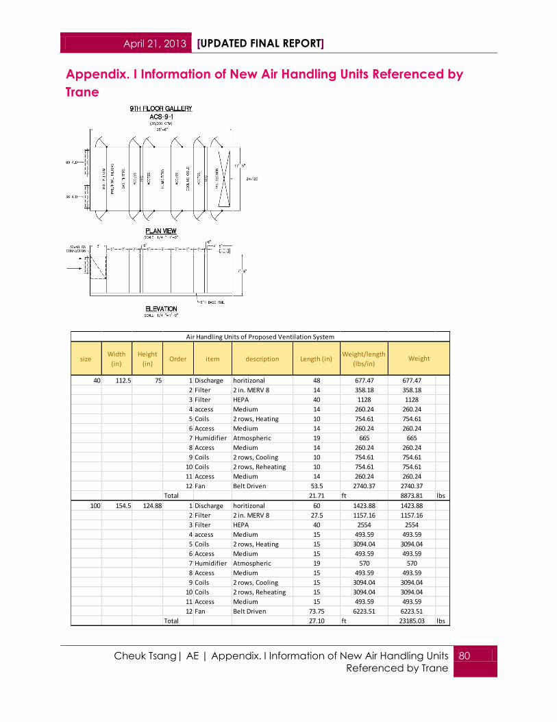
April 21, 2013 [UPDATED FINAL REPORT]
Cheuk Tsang| AE | Appendix. I Information of New Air Handling Units
Referenced by Trane
80
Appendix. I Information of New Air Handling Units Referenced by
Trane
sizeWidth
(in)
Height
(in)Order item description Length (in)
Weight/length
(lbs/in)
40 112.5 75 1 Discharge horitizonal 48 677.47 677.47
2 Filter 2 in. MERV 8 14 358.18 358.18
3 Filter HEPA 40 1128 1128
4 access Medium 14 260.24 260.24
5 Coils 2 rows, Heating 10 754.61 754.61
6 Access Medium 14 260.24 260.24
7 Humidifier Atmospheric 19 665 665
8 Access Medium 14 260.24 260.24
9 Coils 2 rows, Cooling 10 754.61 754.61
10 Coils 2 rows, Reheating 10 754.61 754.61
11 Access Medium 14 260.24 260.24
12 Fan Belt Driven 53.5 2740.37 2740.37
Total 21.71 ft 8873.81 lbs
100 154.5 124.88 1 Discharge horitizonal 60 1423.88 1423.88
2 Filter 2 in. MERV 8 27.5 1157.16 1157.16
3 Filter HEPA 40 2554 2554
4 access Medium 15 493.59 493.59
5 Coils 2 rows, Heating 15 3094.04 3094.04
6 Access Medium 15 493.59 493.59
7 Humidifier Atmospheric 19 570 570
8 Access Medium 15 493.59 493.59
9 Coils 2 rows, Cooling 15 3094.04 3094.04
10 Coils 2 rows, Reheating 15 3094.04 3094.04
11 Access Medium 15 493.59 493.59
12 Fan Belt Driven 73.75 6223.51 6223.51
Total 27.10 ft 23185.03 lbs
Weight
Air Handling Units of Proposed Ventilation System
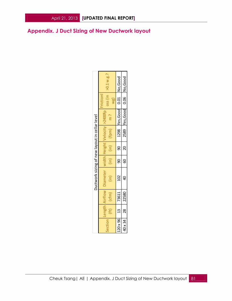
April 21, 2013 [UPDATED FINAL REPORT]
Cheuk Tsang| AE | Appendix. J Duct Sizing of New Ductwork layout 81
Appendix. J Duct Sizing of New Ductwork layout
Sect
ion
Len
gth
(ft)
Air
flo
w
(cfm
)
Dia
me
ter
(in
)
wid
th
(in
)
He
igh
t
(in
)
Ve
loci
ty
(fp
m)
>240
0fp
m ?
Fric
tio
nl
oss
(in
wg)
>0.1
w.g
.?
120
x 96
1373
611
102
9090
1298
Yes,
Go
od
0.01
No
,Go
od
40 x
34
2822
580
4060
2025
89Ye
s,G
oo
d0.
06N
o,G
oo
d
Du
ctw
ork
siz
ing
of
ne
w la
you
t in
ce
llar
leve
l

April 21, 2013 [UPDATED FINAL REPORT]
Cheuk Tsang| AE | Appendix. J Duct Sizing of New Ductwork layout 82

April 21, 2013 [UPDATED FINAL REPORT]
Cheuk Tsang| AE | Appendix. J Duct Sizing of New Ductwork layout 83
Sect
ion
Len
gth
(ft)
Air
flo
w
(cfm
)
Dia
me
ter
(in
)
wid
th
(in
)
He
igh
t
(in
)
Ve
loci
ty
(fp
m)
>240
0fp
m ?
Fric
tio
nlo
ss (
in w
g)
>0.1
w.g
.?
Pre
ssu
re
Loss
Pat
h
1 (i
n w
g)
Pre
ssu
re
Loss
Pat
h
2 (i
n w
g)
Pre
ssu
re
Loss
Pat
h
3 (i
n w
g)
Pre
ssu
re
Loss
Pat
h
4 (i
n w
g)
Pre
ssu
re
Loss
Pat
h
5 (i
n w
g)
Pre
ssu
re
Loss
Pat
h
6 (i
n w
g)
Ad
de
d
0-7
25.0
040
000
6032
8820
38.2
17Ye
s,G
oo
d0.
03N
o,G
oo
d0.
030.
03
7-8
8.50
3125
660
3288
1592
.662
Yes,
Go
od
0.01
No
,Go
od
0.01
8-9
1131
256
6032
8815
92.6
62Ye
s,G
oo
d0.
01N
o,G
oo
d0.
01
1-3
2.5
7814
4448
3274
0.39
06Ye
s,G
oo
d0.
01N
o,G
oo
d0.
01
3-4
878
1444
4832
740.
3906
Yes,
Go
od
0N
o,G
oo
d0
4-5
778
1444
4832
740.
3906
Yes,
Go
od
0N
o,G
oo
d0
5-6
1278
1444
4832
740.
3906
Yes,
Go
od
0N
o,G
oo
d0
0-18
1439
070
6032
8819
90.8
28Ye
s,G
oo
d0.
04N
o,G
oo
d0.
04
18-1
913
1953
539
4030
2356
.009
Yes,
Go
od
0.04
No
,Go
od
0.04
19-2
116
1953
539
4030
2356
.009
Yes,
Go
od
0.04
No
,Go
od
0.04
Y
21-2
213
.598
3533
4818
1656
.683
Yes,
Go
od
0.02
No
,Go
od
0.02
Y
11-1
240
1953
543
4830
1938
.069
Yes,
Go
od
0.05
No
,Go
od
0.05
0.05
12-1
34.
519
535
4340
1419
38.0
69Ye
s,G
oo
d0.
01N
o,G
oo
d0.
010.
01
13-1
416
.519
535
3960
2423
56.0
09Ye
s,G
oo
d0.
01N
o,G
oo
d0.
010.
01
14-1
515
1953
543
6024
1938
.069
Yes,
Go
od
0.07
No
,Go
od
0.07
0.07
Y
15-1
67
9700
3246
1817
37.6
59Ye
s,G
oo
d0.
05N
o,G
oo
d0.
05Y
15-1
718
.598
3530
3025
2004
.586
Yes,
Go
od
0.1
No
,Go
od
0.1
Y
Tota
l 0.
060.
050.
150.
20.
25
Re
turn
uct
wo
rk s
izin
g o
f n
ew
layo
ut

April 21, 2013 [UPDATED FINAL REPORT]
Cheuk Tsang| AE | Appendix. J Duct Sizing of New Ductwork layout 84

April 21, 2013 [UPDATED FINAL REPORT]
Cheuk Tsang| AE | Appendix. J Duct Sizing of New Ductwork layout 85
Sect
ion
Len
gth
(ft)
Air
flo
w
(cfm
)
Dia
me
ter
(in
)
wid
th
(in
)
He
igh
t
(in
)
Ve
loci
ty
(fp
m)
>240
0fp
m ?
Fric
tio
nlo
ss (
in w
g)
>0.1
w.g
.?
Pre
ssu
re
Loss
Pat
h
1 (i
n w
g)
Pre
ssu
re
Loss
Pat
h
2 (i
n w
g)
Pre
ssu
re
Loss
Pat
h
3 (i
n w
g)
Pre
ssu
re
Loss
Pat
h
4 (i
n w
g)
Pre
ssu
re
Loss
Pat
h
5 (i
n w
g)
Ad
de
d
0-3
319
535
4348
3019
38Ye
s,G
oo
d0
No
, Go
od
0.00
0.00
0.00
0.00
0.00
Y
3-4
1219
535
4348
3019
38Ye
s,G
oo
d0.
01N
o, G
oo
d0.
010.
010.
010.
010.
01Y
4-35
0.5
3907
072
7260
1383
Yes,
Go
od
0.02
No
, Go
od
0.02
0.02
0.02
0.02
0.02
Y
35-2
140
1619
043
4830
1606
Yes,
Go
od
0.08
No
, Go
od
0.08
0.08
21-2
22
1619
043
4830
1606
Yes,
Go
od
0N
o, G
oo
d0.
000.
00
22-3
22.
512
690
4360
2412
59Ye
s,G
oo
d0.
01N
o, G
oo
d0.
010.
01
32-3
38.
512
690
4360
2412
59Ye
s,G
oo
d0
No
, Go
od
0.00
0.00
VA
VYe
s,G
oo
d0.
2Ye
s, B
ad0.
20
33-3
410
1269
037
5420
1700
Yes,
Go
od
0.01
No
, Go
od
0.01
22-2
32
3500
2130
1214
56Ye
s,G
oo
d0
No
, Go
od
0.00
23-2
47.
535
0021
3012
1456
Yes,
Go
od
0.01
No
, Go
od
0.01
RH
CYe
s,G
oo
d0.
15Ye
s, B
ad0.
15
24-2
52
3500
3336
2459
0Ye
s,G
oo
d0
No
, Go
od
0.00
25-2
67
3500
3336
2459
0Ye
s,G
oo
d0
No
, Go
od
0.00
26-2
72
3500
2418
2611
15Ye
s,G
oo
d0.
03N
o, G
oo
d0.
03
27-2
86
3500
2418
2611
15Ye
s,G
oo
d0.
01N
o, G
oo
d0.
01
29-3
06.
7535
0024
1826
1115
Yes,
Go
od
0.04
No
, Go
od
0.04
30-3
180
3500
2630
1895
0Ye
s,G
oo
d0.
04N
o, G
oo
d0.
04
35-5
12.5
1642
043
4830
1629
Yes,
Go
od
0.01
No
, Go
od
0.00
0.01
0.01
Y
5-6
216
420
3636
2823
24Ye
s,G
oo
d0
No
, Go
od
0.00
0.00
0.00
Y
6-7
316
420
3636
2823
24Ye
s,G
oo
d0.
01N
o, G
oo
d0.
000.
010.
01Y
7-8
4811
180
4348
3011
09Ye
s,G
oo
d0.
02N
o, G
oo
d0.
00Y
8-9
37.5
1118
043
4830
1109
Yes,
Go
od
0.02
No
, Go
od
0.00
Y
7-10
252
4033
3624
883
Yes,
Go
od
0N
o, G
oo
d0.
000.
00
10-1
18.
7541
2023
2616
1429
Yes,
Go
od
0.07
No
, Go
od
0.07
VA
VYe
s,G
oo
d0.
2Ye
s, B
ad
11-1
20.
541
2023
2616
1429
Yes,
Go
od
0.01
No
, Go
od
0.01
12-1
314
.541
2036
4026
583
Yes,
Go
od
0.01
No
, Go
od
0.01
13-1
424
.541
2030
4018
840
Yes,
Go
od
0.01
No
, Go
od
0.01
10-1
57.
511
2033
3624
189
Yes,
Go
od
0N
o, G
oo
d0.
00
15-1
611
1120
2020
1651
4Ye
s,G
oo
d0
No
, Go
od
0.00
RH
CYe
s,G
oo
d0.
15Ye
s, B
ad0.
15
16-1
710
1120
2020
1651
4Ye
s,G
oo
d0
No
, Go
od
0.00
VA
VYe
s,G
oo
d0.
2Ye
s, B
ad0.
20
17-1
810
.511
2020
2016
514
Yes,
Go
od
0N
o, G
oo
d0.
00
18-1
924
.511
2020
2016
514
Yes,
Go
od
0.01
No
, Go
od
0.01
19-2
036
1120
1720
1271
1Ye
s,G
oo
d0.
02N
o, G
oo
d0.
02
Tota
l 0.
330.
400.
030.
150.
43
Sup
ply
du
ctw
ork
siz
ing
of
ne
w la
you
t

April 21, 2013 [UPDATED FINAL REPORT]
Cheuk Tsang| AE | Appendix. K Structural System Check 86
Appendix. K Structural System Check
Deck Check
Area
9th floor 4454 sf
Original deck 3"-18 guage composite metal deck
3.25 " lightweight concrete
total thickness 6.25
Load assumption
ductwork and pipe 15 psf
fan 1000 lbs/ea
AHUs 9000 lbs/ea
HV 1500 lbs/ea
Load calculation
live load 75 psf from drawing
ductwork and pipe 15 psf
Steel 12 psf
Mechanical equipment load
equipment weight quantiity total
lbs lbs
fan 1000 3 3000
AHU 9000 2 18000
HVs 1500 3 4500
total 25500 lbs
total/total area 5.72519084 psf
total distributed load 107.7251908
Deck type thickness (in) V_a (lbs/ft) F_y (ksi)
3VLI 18 0.0474 4729 50
Total slab depth deck type
SDI Max unshored
clear span (ft)
superimposed
live load (psf)
6.25 3VLI 18 15 191 11.5'
AAM layout
6.25 3" 18 guage 11.5 107.7251908
Conclusion: Checked OK
Deck Check

April 21, 2013 [UPDATED FINAL REPORT]
Cheuk Tsang| AE | Appendix. K Structural System Check 87
Beams
De
ad lo
ad
du
ctw
ork
an
d p
ipe
15
psf
De
ck46
psf
slab
50p
sf
Me
chan
ical
eq
uip
me
nt
load
5.
7251
9084
psf
tota
l dis
trib
ute
d lo
ad
116.
7251
908
psf
Influ
en
ce
Are
a o
f B
ea
ms
De
ad
Lo
ad
Dis
trib
utio
n
Live
load
live
load
75
psf
Liv
e L
oa
d D
istr
ibu
tio
n

April 21, 2013 [UPDATED FINAL REPORT]
Cheuk Tsang| AE | Appendix. K Structural System Check 88
be
am
shap
e
self
we
igh
t
(lb
)
Span
Le
ngt
h
De
ad
load
(p
sf)
De
ad
load
of
wal
l
add
itio
na
l lo
adw
L To
tal
Vu
Equ
atio
n
Mu
Equ
atio
nV
uφ
_v V
_px
Yes/
No
Mu
φ
_n
M_p
xYe
s/N
o
1W
21x4
444
4010
116.
7252
150
2.47
08(w
L)*L
/2(w
L)*L
^2/8
12.3
5421
7Ye
s30
.885
358
Yes
2W
21x4
444
4020
015
2.08
2302
4.89
5102
(wL)
*L/2
(wL)
*L^2
/848
.951
0221
7Ye
s24
4.75
5135
8Ye
s
3W
21x4
444
4020
015
2.08
2302
4.89
5102
(wL)
*L/2
(wL)
*L^2
/848
.951
0221
7Ye
s24
4.75
5135
8Ye
s
4W
21x4
444
4020
015
2.08
2302
4.89
5102
(wL)
*L/2
(wL)
*L^2
/848
.951
0221
7Ye
s24
4.75
5135
8Ye
s
5W
21x4
444
2010
116.
7252
02.
0535
02(w
L)*L
/2(w
L)*L
^2/8
10.2
6751
94.5
Yes
25.6
6878
125
Yes
6W
21x4
444
2010
116.
7252
02.
0535
02(w
L)*L
/2(w
L)*L
^2/8
10.2
6751
94.5
Yes
51.3
3756
125
Yes
7W
10x3
333
1810
116.
7252
1.84
0232
(wL)
*L/2
(wL)
*L^2
/89.
2011
684
.7Ye
s46
.005
814
5Ye
s
dis
trib
ute
d lo
ad
Be
am
be
am
shap
e
self
we
igh
t
(lb
)
Span
Le
ngt
h
De
ad
load
(p
sf)
De
ad
load
of
wal
l
add
itio
na
l lo
adw
L To
tal
Vu
Equ
atio
n
Mu
Equ
atio
nV
u
φ_v
V_p
xYe
s/N
oM
u
φ_n
M_p
xYe
s/N
oB
_ft_
f
B_f
/2/t
_
w<
9.15
?t_
wh
h/t
_w<9
0.5?
a W
30
x 90
9015
.548
015
0.71
9132
2.11
7132
(wL)
*L/2
(wL)
*L^2
/850
.811
1746
3Ye
s60
9.73
411
70Ye
s10
.50.
677.
8358
21Ye
s0.
5229
55.7
6923
Yes
b
W 1
4 x
2222
1010
116.
7252
00
2.02
7102
(wL)
*L/2
(wL)
*L^2
/810
.135
5194
.5Ye
s25
.338
7812
5Ye
s5
0.33
57.
4626
87Ye
s0.
2313
.458
.260
87Ye
s
c W
16
x 26
2610
2411
6.72
520
02.
0319
02(w
L)*L
/2(w
L)*L
^2/8
24.3
8283
105
Yes
146.
297
166
Yes
5.53
0.34
58.
0144
93Ye
s0.
2515
.562
Yes
dW
30
x 90
9010
4011
6.72
520
02.
1087
02(w
L)*L
/2(w
L)*L
^2/8
42.1
7405
463
Yes
421.
7405
1170
Yes
10.5
0.67
7.83
5821
Yes
0.52
2955
.769
23Ye
s
e fW
24
x 68
6810
4011
6.72
520
02.
0823
02(w
L)*L
/2(w
L)*L
^2/8
41.6
4605
295
Yes
416.
4605
664
Yes
8.97
0.58
57.
6666
67Ye
s0.
415
23.1
55.6
6265
Yes
W 2
7 x
8484
1040
116.
7252
00
2.10
1502
(wL)
*L/2
(wL)
*L^2
/842
.030
0536
8Ye
s42
0.30
0591
5Ye
s7.
78Ye
s52
.7Ye
s
gW
30
x 90
9010
4011
6.72
520
02.
1087
02(w
L)*L
/2(w
L)*L
^2/8
42.1
7405
463
Yes
421.
7405
1170
Yes
10.5
0.67
7.83
5821
Yes
0.52
2955
.769
23Ye
s
hW
24
x 68
6810
4011
6.72
520
02.
0823
02(w
L)*L
/2(w
L)*L
^2/8
41.6
4605
295
Yes
416.
4605
664
Yes
8.97
0.58
57.
6666
67Ye
s0.
415
23.1
55.6
6265
Yes
i jW
24
x 68
6810
4011
6.72
520
02.
0823
02(w
L)*L
/2(w
L)*L
^2/8
41.6
4605
295
Yes
416.
4605
664
Yes
8.97
0.58
57.
6666
67Ye
s0.
415
23.1
55.6
6265
Yes
kW
24
x 68
6810
4011
6.72
520
02.
0823
02(w
L)*L
/2(w
L)*L
^2/8
41.6
4605
295
Yes
416.
4605
664
Yes
8.97
0.58
57.
6666
67Ye
s0.
415
23.1
55.6
6265
Yes
Be
am
dis
trib
ute
d lo
ad
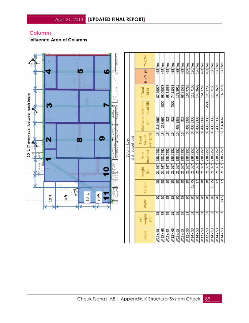
April 21, 2013 [UPDATED FINAL REPORT]
Cheuk Tsang| AE | Appendix. K Structural System Check 89
Columns
Influence Area of Columns
shap
e
self
we
igh
t
(lb
)
Wid
th
Len
gth
h
eig
ht
(ft)
De
ad
load
(p
sf)
De
ad
load
of
wal
l (p
sf)
Wal
l are
a
(sf)
add
itio
na
l lo
ad (
lb)
P T
ota
l
(Mlb
)φ
_v V
_px
Yes/
No
W12
x 6
5 65
1020
21.6
6723
8.72
5215
216.
6667
87.2
9077
492
Yes
W 1
2 x
6565
1020
21.6
6723
8.72
5215
216.
667
9000
98.0
9078
492
Yes
W12
x 6
5 65
1510
21.6
6723
8.72
5215
325
68.8
1558
492
Yes
W 1
2 x
6565
1510
21.6
6723
8.72
5215
325
4500
74.2
1558
492
Yes
W12
x 6
565
2020
21.6
6723
8.72
5215
433.
3333
172.
8915
492
Yes
W12
x 6
565
1510
21.6
6723
8.72
5215
325
68.8
1558
492
Yes
W 1
2 x
5353
2020
21.6
6723
8.72
520
433.
3333
164.
7795
307
Yes
W 1
4 x
5353
2013
.75
21.6
6723
8.72
520
433.
3333
113.
7166
186
Yes
W 1
4 x
5353
2017
21.6
6723
8.72
520
433.
3333
140.
2693
186
Yes
W 1
2 x
5353
2020
21.6
6723
8.72
520
433.
3333
164.
7795
492
Yes
W 1
2 x
5353
2020
21.6
6723
8.72
520
433.
3333
4500
170.
1796
492
Yes
W 1
4 x
5353
2013
.75
21.6
6723
8.72
520
433.
3333
113.
7166
186
Yes
W 1
4 x
5353
2017
21.6
6723
8.72
5243
3.33
3314
0.26
9318
6Ye
s
W 1
4 x
5353
14.5
1721
.667
238.
7252
1531
4.16
6710
7.72
9218
6Ye
s
Co
lum
n L
oad
dis
trib
ute
d lo
ad

April 21, 2013 [UPDATED FINAL REPORT]
Cheuk Tsang| AE | Appendix. L Noise Criteria Charts
90
Appendix. L Noise Criteria Charts
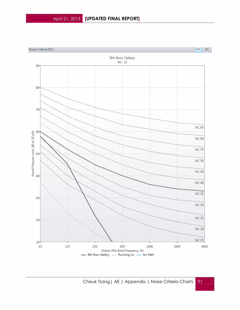
April 21, 2013 [UPDATED FINAL REPORT]
Cheuk Tsang| AE | Appendix. L Noise Criteria Charts
91

April 21, 2013 [UPDATED FINAL REPORT]
Cheuk Tsang| AE | Appendix. L Noise Criteria Charts
92

April 21, 2013 [UPDATED FINAL REPORT]
Cheuk Tsang| AE | Appendix. L Noise Criteria Charts
93

April 21, 2013 [UPDATED FINAL REPORT]
Cheuk Tsang| AE | MAE Course Relation 94
MAE Course Relation The MAE courses related to this project are:
AE 557 Centralized Cooling System:
The ideas of absorption refrigeration in this course help to understand the impact to
other mechanical components and the installation requirement of absorption chillers.
Also, the lecture of AHRI Standard 550/590 and ASHRAE Standard 90.1 explains the
potential energy saving of operating with multiple chillers instead of one. Third, this
course mentions the requirements and needs of mechanical room layout.
AE 555 Building Control System:
This course provides different search methods that can be applied on HVAC operation,
such as increasing the efficiency of HVAC system by changing the combination of mass
flow rates, temperature setpoints, and part load ratios. This concept helps to find the
cost effective combination of electric and absorption chillers, and also the well
balanced layout of the mechanical room on 9th floor.
AE 551 Combined Heat and Power:
This course provides information of today fuel economy and theories of different
cogeneration operations. It significantly gives the analysis of this project more
alternatives of redesigning the HVAC system.