1

GSA Data Repository 2018146

Unzipping continents and the birth of microcontinents

N. E. Molnar, A. R. Cruden, P. G. Betts.

This PDF file includes:

Additional remarks: types of lithospheric weaknesses Materials and Methods Figs. DR1 to DR4

2

Additional remarks: types of lithospheric weaknesses

Many divergent tectonic settings occur in the presence of pre-existing structures in

the lithosphere. These structures include lateral variations in lithospheric thickness that

perturb mantle flow (e.g., Ebinger & Sleep, 1998), weaknesses within the lithospheric

mantle or crust caused by activity of mantle plumes or hot spots (Corti, 2008), mantle

penetrating shear zones characterised by reduced grain size (Heron et al., 2016), or

inherited mechanical anisotropies with lattice preferred orientation of olivine crystals

(Tommasi & Vauchez, 2001). Because these features lead to linear zones of anomalously

weak or strong material within the lithosphere we refer to them as “rheological

heterogeneities”. For the specific case addressed in the main body of this manuscript, the

roughly linear geometry may be related to the migration of plume material through

thinned sections of lithosphere which, in turn, are associated with roughly linear ancient

rifts or areas of intense extensional deformation (Ebinger and Sleep, 1998) (DR4).

Crustal heterogeneities are commonly associated with pre-existing basement faults

(Wilson et al., 2010), suture zones (Stern & Johnson, 2010) and orogenic belts (Vauchez

et al., 1997), which often juxtapose different lithospheric blocks with different ages and

mechanical properties. These heterogeneities localize strain and consequently influence

where and how the lithosphere deforms, ultimately affecting tectonic plate kinematics

and strain distribution (Molnar et al., 2017).

References: Stern, R.J., and Johnson, P., 2010, Continental lithosphere of the Arabian Plate: A

geologic, petrologic, and geophysical synthesis: Earth-Science Reviews, v. 101, p. 29–

67, doi: 10.1016/j.earscirev.2010.01.002.

3

Vauchez, A., Barruol, G., and Tommasi, A., 1997, Why do continents break-up parallel

to ancient orogenic belts?: Terra Nova, v. 9, p. 62–66, doi: 10.1111/j.1365-

3121.1997.tb00003.x.

Wilson, R.W., Holdsworth, R.E., Wild, L.E., McCaffrey, K.J.W., England, R.W., Imber,

J., and Strachan, R.A., 2010, Basement-influenced rifting and basin development: a

reappraisal of post-Caledonian faulting patterns from the North Coast Transfer Zone,

Scotland: Continental Tectonics and Mountain Building: The Legacy of Peach and

Horne, v. 335, p. 795–826, doi: 10.1144/SP335.32.

Materials and Methods

All models were constructed using a length scale ratio of 4 x 10-7, meaning that 1

cm in the models represents 25 km in nature. The initial 44 x 44 x 3 cm dimension of all

models allowed to simulate the deformation of large lithospheric domains on Earth

(~1100 x ~1100 km x ~80 km) submitted to rotational extensional kinematics. During

assembly, the three-layer, brittle-ductile, model lithospheric plates were confined by two

bottomless U-shaped acrylic walls that allowed the model lithosphere to float isostatically

on a fluid model asthenosphere, contained within a 65 x 65 x 20 cm acrylic tank (Fig. 2).

The brittle upper crust was modelled using a mixture of quartz sand and hollow ceramic

microspheres and the ductile lower crust was replicated using silicone gum

(polydimethylsiloxane). The model lithospheric mantle was prepared by mixing the same

silicone gum with black modelling clay and hollow glass microspheres in appropriate

proportions so as to obtain suitable up-scaled values for viscosity and density (Molnar et

al., 2017). Similarly, a mixture of silicone and black modelling clay was used to model a

weaker lithospheric mantle, which was prepared separately and incorporated into the

4

reference lithospheric mantle during model construction. A solution of Natrosol® 250 HH

and sodium chloride in water was used to model the low viscosity asthenospheric mantle.

Complete scaling and physical property information of all the materials can be found in

Molnar et al. (2017). Densities of the model ductile mixtures were calculated through the

water displacement method, while the density of the model asthenospheric mantle was

calculated using an Anton Paar DMA 4500 M density meter. The rheological properties

of all materials and mixtures were tested and measured in the laboratory using an Anton

Paar Physica MCR-301 parallel plate rheometer to ensure a suitable similarity with the

natural prototype (Molnar et al., 2017).

A 5 cm wide linear weak zone was incorporated in the lithospheric mantle to

investigate the mechanics of rifting in a heterogeneous lithosphere. The orientation of the

linear weakness with respect to the initial extension direction was varied between

experiments to analyze the influence of its obliquity. A rotational extensional boundary

condition was imposed to study the interaction of rifts propagating towards a fixed pole

of rotation in the presence of linear rheological heterogeneities. The progressive

anticlockwise rotation was created by fixing one U-shaped wall to the side of the acrylic

tank and pulling the other with a linear actuator at a constant divergence rate of ~1.4-4 m

s-1, which scales to natural velocities of ~16 mm yr-1, as estimated for the Southern Red

Sea (Bosworth et al., 2005; McClusky et al., 2010). The properties of the analogue

materials set dimensionless viscosity and density ratios which, in turn, define a time scale

factor such that 1 h in the experiment corresponds to ~0.8 Ma in nature (Molnar et al.,

2017). All models were run for 38 h, which corresponds to ~30 Ma and ~45% extension

in nature.

5

The experiments were monitored using a particle image velocimetry (PIV) system.

Sequential stereoscopic and top-view images were taken at 2 min intervals and processed

using a stereo cross correlation technique (Adam et al., 2005) to obtain digital elevation

models (DEMs) and high-resolution (≥0.1 mm) displacement fields. Color scheme

chosen to illustrate topography as yellow and maroon for topographic highs and blue for

low elevations and/or topographic depressions. Precise spatiotemporal measurements of

differential and cumulative strain were subsequently computed and used to plot

differential normal surface strain (Molnar et al., 2017), which are overlaid on the

evolutionary cross-sections in Figure 3 and Figures DR2 and DR3.

6

Fig. DR1. Additional examples of microcontinents and isolated continental segments.

Bathymetric and topographic maps with locations of selected end-members (pink) and

failed break-up basins (yellow). A: Continental ribbons (Peron-Pinvidic and Manatschal,

2010) at both conjugate margins of the North Atlantic Ocean: Orphan basin (OB),

Orphan Knoll (OK) and Flamish Cap (FC) at the Newfoundland margin and Porcupine

Bank (PB) and Galicia Bank (GB) at the Iberian margin. B: Sri Lanka (SL) and Mauritian

continental fragments in the Indian Ocean: Seychelles (S), Saya de Malha (SdM),

Nazaret (NA), Cargados-Carajos (CC), Mauritius (MA) and Chagos (CH). C: Failed

break-up basins (yellow), Macclesfield Bank (MB) and Reed Bank (RB) in the South

China Sea. D: Southern Ocean continental fragments: Elan Bank (EB) and Kerguelen

Plateau (KP). E: South Indian Ocean continental fragments and ridges: Broken Ridge

(BR), Gulden Draak microcontinent (GD), Batavia microcontinent (B), Zenith Plateau

(ZP), Wallaby Plateau (WP) and Naturaliste Plateau (NP). Ocean-continent boundary is

represented by a dashed red line.

AA

B C

D E

53.6˚N1.5˚E

60˚W35.6˚N

10˚N85˚E

41˚E24˚S

29˚N135˚E

97˚E2˚N

41˚S97˚E

21˚E71˚S

12˚S121˚E

83˚E37˚S

KP

EB

KP

EB

WP

ZP

B

GD

BRNP

WP

ZP

MBMBRBRB

B

GD

BRNP

Topobathymetry

m-3000 -2000 -1000 0 1000 2000 3000

NN

NN

NN

NorthAmerica

Europe

Asia

Australia

Antarctica

NorthAmerica

Europe

FC

PB

FC

OKOB PB

GB

NA

SdM

CC

MA

CH

S

NA

SdM

CC

MA

CH

SLSL

S

NN Africa Africa

Asia

Australia

Antarctica

NN

Fig. DR1

7

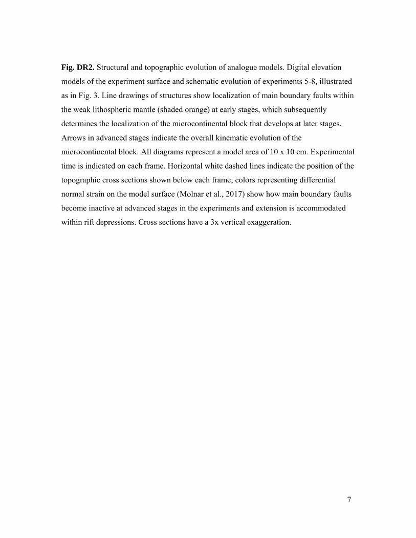
Fig. DR2. Structural and topographic evolution of analogue models. Digital elevation

models of the experiment surface and schematic evolution of experiments 5-8, illustrated

as in Fig. 3. Line drawings of structures show localization of main boundary faults within

the weak lithospheric mantle (shaded orange) at early stages, which subsequently

determines the localization of the microcontinental block that develops at later stages.

Arrows in advanced stages indicate the overall kinematic evolution of the

microcontinental block. All diagrams represent a model area of 10 x 10 cm. Experimental

time is indicated on each frame. Horizontal white dashed lines indicate the position of the

topographic cross sections shown below each frame; colors representing differential

normal strain on the model surface (Molnar et al., 2017) show how main boundary faults

become inactive at advanced stages in the experiments and extension is accommodated

within rift depressions. Cross sections have a 3x vertical exaggeration.

37 h29.6 h9.5 h

20 h8.4 h3.3 h

13.5 h6.6 h3.3 h

19.6 h8.3 h2.3 h

37 h29.6 h9.5 h

20 h8.4 h3.3 h

13.5 h6.6 h3.3 h

19.6 h8.3 h2.3 h

Time

EarlyEarly IntermediateIntermediate AdvancedAdvanced

NN

NN

NN

NN

MO

DE

L 5

MO

DE

L 5

MO

DE

L 6

MO

DE

L 6

MO

DE

L 7

MO

DE

L 7

MO

DE

L 8

MO

DE

L 8

Fig. DR2

8

Fig. DR3. Structural and topographic evolution of analogue models. Digital elevation

models of the experiment surface and schematic evolution of experiments 9-10-11,

illustrated as in Fig. 3 and DR2. Line drawings of structures show localization of main

boundary faults within the weak lithospheric mantle (shaded orange) at early stages,

which subsequently determines the localization of the microcontinental block that

develops at later stages. Arrows in advanced stages indicate the overall kinematic

evolution of the microcontinental block. All diagrams represent a model area of 10 x

10 cm. Experimental time is indicated on each frame. Horizontal white dashed lines

indicate the position of the topographic cross sections shown below each frame; colors

representing differential normal strain on the model surface (Molnar et al., 2017)

show how main boundary faults become inactive at advanced stages in the

experiments and extension is accommodated within rift depressions. Cross sections

have a 3x vertical exaggeration.

20.8 h4.2 h2.5 h

20.8 h8.3 h4.2 h

20.8 h4.2 h2.5 h

20.8 h8.3 h4.2 h

Time

EarlyEarly IntermediateIntermediate AdvancedAdvanced

NN

NN

NN

MO

DE

L 11

MO

DE

L 11

MO

DE

L 9

MO

DE

L 9

MO

DE

L 10

MO

DE

L 10

20 h8.1 h1.6 h 20 h8.1 h1.6 h

Fig. DR3

9

Fig. DR4. Red Sea-Gulf of Aden rift system comparison with analogue model. A:

Topographic and bathymetric map of the Red Sea-Gulf of Aden rift system. Yellow

arrows show GPS-derived velocities of Arabia with respect to Eurasia (McClusky et al.,

2010), demonstrating the anticlockwise rotation of Arabia. Danakil Block (DB)

highlighted in orange. Area shaded in red represents the region affected by the northward

channeling of Afar hotspot (Chang et al., 2011), possibly causing thermal weakening on

the lithosphere. Solid black line indicates the location of the cross section shown in (B).

B: Bathymetry and topography with a 10x vertical exaggeration and shear wave velocity

cross-sections across the Red Sea and Danakil Block, showing the approximate location

of the velocity perturbations below the southern Red Sea and its correlation with the

position of the Danakil Block (DB). Position of the cross-section in a schematic regional

setting is indicated in the left panel. C: Model 1 elevation profile with a 10x vertical

exaggeration and approximate location of the rheological weakness in the lithospheric

mantle and its correlation with the position of the intra rift block (IRB). Position of the

cross-section in the model was chosen for direct comparison with the prototype and is

indicated in the left panel.

X X’

km0

3

300

AA B

C

Y Y’Y

0

3

30Topobathymetry

m-3000 -2000 -1000 0 1000 2000 3000

36˚N65˚E

5.5˚N22˚E

500 km

NN

Africa

Arabia

-300 m/s3000

DBDB

Afr.

DB

Ar.

IRB

mm

Y

Y’

X

X’

Fig. DR4