unveiling rival’s offering prices in electricity markets
TRANSCRIPT

Unveiling rival’s offering prices inElectricity Markets
José Andrés Cortés Granell(s161339)
Supervised by: Pierre PinsonKongens Lyngby 2018

DTU ElektroDepartment of Electrical EngineeringTechnical University of Denmark
Elektrovej, Building 3252800 Kongens Lyngby, DenmarkPhone (+45) 45253500Fax (+45) 45886111E-mail:[email protected]/cee

SummaryIn this Master Thesis, several alternatives are proposed in order to reveal offering pricesin a spot market. This proposal to obtain hidden information within a system is con-sidered as a very powerful mean to acquire a competitive advantage when proposing amarket strategy.
Due to the opacity found in terms of methods to perform this exercise, the applica-tion proposed in this project is considered novel. Many proposals related to carrying outa strategic offering have been found although they result in nothing similar to what isproposed in this project. Taking as reference some aspects of these works already done,it is suggested as an improvement the use of a recursive filter.
For the purpose of obtaining of results, the modeling of a pair of representative elec-trical markets has been developed. Through them, outcomes will be generated in orderto check if the suggested methods work properly. As a first step, an Inverse OptimizationProblem will be applied to an electric market with three nodes and two interconnections.The outputs obtained through this methodology will be taken as a reference in order toimprove them along an algorithm with simpler formulation.
Further on, an Ensemble Kalman Filter will be applied with the objective of reachingmore feasible results than those obtained in the previous methodology. To do this, thesame market will be used but reduced to a single node, although with more participants.In order to verify its robustness, three different situations will be proposed. In the firstscenario, the EnKF model will remain static, which will lead to a better understandingof how the algorithm behaves. In the second scenario, the model will change to dynamic,and its parameters will be updated depending on the needs of the market. Finally, athird scenario will be proposed taking into account the formulation of the second scenario,although with different market conditions. In order to study the changes in demand, suchas a failure in an interconnection or even a transition between year’s seasons, extremechanges will be made between periods of simulation.

ii

ResumenEn este proyecto final de máster, se proponen varias alternativas con el fin de revelarprecios de oferta en un mercado del tipo spot. Esta propuesta de obtener informaciónescondida dentro de un sistema, se considera como un medio muy potente para poderadquirir una ventaja competitiva al proponer una estrategia de mercado.
Debido a la opacidad encontrada en cuanto a la metodología se refiere para realizardicho ejercicio, la aplicación propuesta en este trabajo es considerada del tipo novel.Muchas publicaciones relacionadas con optimizar una oferta estratégica se han encon-trado aunque resulten en nada similar a lo propuesto en este proyecto. Tomando comoreferencia algunos aspectos de estos trabajos ya realizados, se propone como mejora eluso de un filtro recursivo.
Para la obtención de resultados, se ha realizado los modelos de un par de mercadoseléctricos representativos. Mediante ellos, se generarán resultados con el fin de podercomprobar si los métodos sugeridos funcionan adecuadamente. En un primer lugar, seaplicará un Problema de Optimización Inverso a un mercado eléctrico con tres nodos ytres interconexiones. Los resultados obtenidos mediante esta metodología, se tendráncomo referencia con el fin de mejorarlos con una formulación mas sencilla y potente.
Finalmente, se aplicará un Ensemble Kalman Filter con el fin de encontrar resultadosmás factibles que en los obtenidos en la metodología anterior. Para ello, se utilizará elmismo mercado pero reducido a un nodo aunque con un mayor número de participantes.Para poder comprobar su robustez, se propondrán tres escenarios distintos. En el primerescenario el modelo del EnKF será estático, lo que conllevará a entender mejor comofunciona el algoritmo. En el segundo escenario, el modelo cambiará a dinámico, y susparámetros se actualizaran dependiendo de las necesidades del mercado. Finalmente,un tercer escenario será propuesto teniendo en cuenta la formulación del escenario dos,pero con unas condiciones de mercado diferentes. Con el fin de estudiar los cambios dedemanda, como puede ser un fallo en una interconexión o incluso un cambio de estacióndel año, se le realizaran cambios bruscos entre periodos de simulación.

iv

PrefaceThis Master thesis was prepared at the department of Electrical Engineering at the Tech-nical University of Denmark in fulfillment of the requirements for acquiring a Master ofScience in Electrical Engineering.
This work will be presented both at the Technical University of Denmark and atthe Polytechnic University of Valencia, as provided for in the agreement for the DoubleDegree program T.I.M.E..
Kongens Lyngby, April 10, 2018
José Andrés Cortés Granell(s161339)

vi

AcknowledgementsI would like to thank Professor Pierre Pinson, supervisor of this Master’s Thesis. Firstly,for showing me the confidence to carry out this project whose theme was partially un-known for me and secondly, for his continuous advice and mentorship along these lastmonths. His comments and suggestions during my work have been highly valuable andconstructive.
I am thankful to both Technical University of Denmark and the Polytechnic Univer-sity of Valencia for all they offered me: resources, facilities, competent and experiencedprofessors and, most important of all, a high quality education. Also, I have to expressparticular gratitude to the TIME (Top Industrial Managers for Europe) Association,which has permitted an agreement between universities offering me a double degreeprogram which gives a unique educational opportunity and extraordinary experience ofpersonal growth.
Last but not least, I want to thank and express deepest gratitude to my family: with-out their constant support and encouragement along these years I would never achievethis double Master degree. M’ho heu donat tot i jo sempre he intentat respondre, siestic ací és per vosaltres, gràcies.

viii

SymbolsPARAMETERS FOR THE INVERSE OPTIMIZATION PROBLEM
Symbol Unit Definition
λGdtnb e/MWh Price offer for power block of the strategic unit at node
n in time period t on day d.
λOdtnb e/MWh Price offer for power block of the rival unit at node n
in time period t on day d.
λOtruenb e/MWh Marginal cost of power block of the rival unit at node
n.
λOinidtnb e/MWh Initial estimation of the marginal cost of power block
of the rival unit at node n in time period t on day d.
λDdtnk e/MWh Price bid of demand block at node n in time period t
on day d.
P Gmaxnb MW Upper bound of power block of the strategic unit at
node n.
P Omaxnb MW Upper bound of power block of the rival unit at node
n.
P Dmaxdtnk MW Upper bound of demand block at node n in time period
t on day d.
P Ginidn MW Total power produced by the strategic unit at node n
in the time period (t=0) prior to day d.
P Oinidn MW Total power produced by the rival unit at node n in
the time period (t=0) prior to day d.
P maxnm MW Transmission capacity of line n-m.

x Symbols
Symbol Unit Definition
Bnm S Susceptance of line n-m.
RGdwnn MW/h Ramp-down limit of the strategic unit at node n.
RGupn MW/h Ramp-up limit of the strategic unit at node n.
ROdwnn MW/h Ramp-down limit of the rival unit at node n.
ROupn MW/h Ramp-up limit of the rival unit at node n.
λMC e/MWh Marginal cost of each company used in the model.
VARIABLES FOR THE MARKET CLEARING PROBLEM
Symbol Unit Definition
P Gdtnb MW Power produced by block b of the strategic unit at node
n in time period t on day d.
P Odtnb MW Power produced by block b of the rival unit at node n
in time period t on day d.
P Ddtnk MW Power consumed by block k of the demand at node n
in time period t on day d.
δdtn Radians Voltage angle of node in time period t on day d.
λdtn e/MWh LMP at node n in time period t on day d (dual vari-able).
VARIABLE FOR THE INVERSE OPTIMIZATION PROBLEM
Symbol Unit Definition
λOdtnb e/MWh Price offer of power block b of the rival unit at node n
in time period t on day d.

Symbols xi
PARAMETERS FOR THE SIMPLE KALMAN FILTER
Symbol Unit Definition
Mt - Constant which permits to propagate the initial state es-timate variable into the a priori state estimate variable ineach time period t.
wt - White noise associated to the error committed when prop-agating the initial state estimate variable in each time pe-riod t.
Qt - Noise covariance of parameter wt.
Ht - Constant which permits to relate the a priori state esti-mate variable with the measurement taken in each timeperiod t.
vt - White noise associated to the error committed when ob-taining the measurement in each time period t.
Rt - Noise covariance of parameter vt
Kt - Kalman Gainer. Reduces the uncertainty in the a posteri-ori state estimate variable and corrects the a priori stateestimate variable.
VARIABLES FOR THE SIMPLE KALMAN FILTER
Symbol Unit Definition
xt e/MWh The a priori state estimate variable in each time periodt. Collects offering prices in the forecasting step.
Pt - Predicted (a priori) estimate covariance associated tothe previous variable in each time period t.
yt e/MWh Observation of the true state in each time period t.
xt e/MWh The a posteriori state estimate variable in each timeperiod t. Collects corrected offering prices in the up-dating step.

xii Symbols
Symbol Unit Definition
Pt - Updated (a posteriori) estimate covariance associatedto the previous variable in each time period t.
PARAMETERS FOR THE ENSEMBLE KALMAN FILTER
Symbol Unit Definition
Mt - Constant matrix which permits to propagate the initialstate estimate variable matrix into the a priori state esti-mate variable matrix in each time period t.
wt - White noise associated to the error committed when prop-agating the initial state estimate variable matrix in eachtime period t.
Qt - Noise covariance of parameter wt.
Et - Parameter which reflects the mean values with respect toeach column given matrix in each time period t. Usedonly with the a priori state estimate variable matrix.
At - Parameter which collects the result of subtracting to thea priori state estimate variable matrix the Et matrix ineach time period t.
Ct - Parameter which collects the sample covariance matrixregarding the a priori state estimate variable in each timeperiod t.
Ht - Constant matrix which permits to relate the a priori stateestimate variable matrix with the simulated measurementmatrix in each time period t.
vt - White noise associated to the error committed when ob-taining the simulated measurement in each time periodt.
Rt - Noise covariance of parameter vt

Symbols xiii
Symbol Unit Definition
Kt - Estimated Kalman Gainer. Reduces the uncertainty inthe a posteriori state estimate variable and corrects the apriori state estimate variable.
VARIABLES FOR THE ENSEMBLE KALMAN FILTER
Symbol Unit Definition
xt e/MWh The a priori state estimate variable matrix in eachtime period t. Collects offering prices in the forecastingstep.
yt e/MWh Simulated observation of the true state in each timeperiod t.
yt e/MWh Observation of the true state in each time period t.
xt e/MWh The a posteriori state estimate variable matrix in eachtime period t. Collects corrected offering prices in theupdating step.
ADDITIONAL PARAMETERS FOR THE ENSEMBLE KALMAN FIL-TER
Symbol Unit Definition
dt - Constant matrix which measures the risk taken by the lastcompany in a market clearing in each time period t.
jt - Constant matrix which extrapolates the risk taken by thelast company in a market clearing to the other partici-pants in each time period t. This constant will multiplymatrix Ht

xiv

NomenclatureSymbol Definition
PCI Projects of Interest
OMIE Operator of the Iberian Energy Market
EPEX The European Power Exchange
GME Electricity Market Manager (Italy)
LMP Local Marginal Price
SMP System’s Marginal Price
S Strategic Producer
O Rival Producer
PQ (Bus) Load Bus
ISO Independent System Operator
KKT Karush-Kuhn-Tucker
EnKF Ensemble Kalman Filter
KF Simple Kalman Filter
PDF Probability Distribution Function
GPS Global Positioning System
CPU Central Processing Unit
MIBEL Iberian Electricity Market

xvi Nomenclature

ContentsSummary i
Resumen iii
Preface v
Acknowledgements vii
Symbols ix
Nomenclature xv
Contents xvii
1 Introduction 1
2 Motivation & Electricity Markets 52.1 Literature Review . . . . . . . . . . . . . . . . . . . . . . . . . . . . . . . 52.2 The Electricity Market . . . . . . . . . . . . . . . . . . . . . . . . . . . . 8
2.2.1 Main Features of Electricity Markets . . . . . . . . . . . . . . . . 82.2.2 The day-ahead Market . . . . . . . . . . . . . . . . . . . . . . . . 92.2.3 The 3-Node Electricity Market . . . . . . . . . . . . . . . . . . . . 10
2.2.3.1 Layout of the Market . . . . . . . . . . . . . . . . . . . . 102.2.3.2 Technical Data from the Grid . . . . . . . . . . . . . . . 112.2.3.3 Strategic and Rival Generating Companies . . . . . . . . 112.2.3.4 Demand . . . . . . . . . . . . . . . . . . . . . . . . . . . 132.2.3.5 Equations . . . . . . . . . . . . . . . . . . . . . . . . . . 152.2.3.6 Outcomes from Clearings . . . . . . . . . . . . . . . . . 15
2.2.4 1-Node Electricity Market . . . . . . . . . . . . . . . . . . . . . . 162.2.4.1 Layout of the Market . . . . . . . . . . . . . . . . . . . . 162.2.4.2 Generating Companies . . . . . . . . . . . . . . . . . . . 172.2.4.3 Other specifications of the Market . . . . . . . . . . . . 19
3 Methods 213.1 Inverse Optimization Problem . . . . . . . . . . . . . . . . . . . . . . . . 21
3.1.1 Introduction . . . . . . . . . . . . . . . . . . . . . . . . . . . . . . 21

xviii Contents
3.1.2 Market Clearing Model . . . . . . . . . . . . . . . . . . . . . . . . 223.1.2.1 Primal Problem Formulation . . . . . . . . . . . . . . . 223.1.2.2 Dual Problem Formulation . . . . . . . . . . . . . . . . 25
3.1.3 Inverse Problem Formulation . . . . . . . . . . . . . . . . . . . . 263.2 Ensemble Kalman Filter . . . . . . . . . . . . . . . . . . . . . . . . . . . 27
3.2.1 Introduction . . . . . . . . . . . . . . . . . . . . . . . . . . . . . . 273.2.2 Basic formulation . . . . . . . . . . . . . . . . . . . . . . . . . . . 28
3.2.2.1 Kalman Filter . . . . . . . . . . . . . . . . . . . . . . . . 283.2.2.2 The Ensemble Kalman Filter . . . . . . . . . . . . . . . 32
3.2.3 Implementation for revealing prices . . . . . . . . . . . . . . . . . 39
4 Results 414.1 Inverse Optimization . . . . . . . . . . . . . . . . . . . . . . . . . . . . . 41
4.1.1 Revealing marginal costs . . . . . . . . . . . . . . . . . . . . . . . 414.1.2 Conclusions . . . . . . . . . . . . . . . . . . . . . . . . . . . . . . 44
4.2 Ensemble Kalman Filter . . . . . . . . . . . . . . . . . . . . . . . . . . . 454.2.1 First estimation . . . . . . . . . . . . . . . . . . . . . . . . . . . . 464.2.2 Initial distributions . . . . . . . . . . . . . . . . . . . . . . . . . . 474.2.3 Revealing offering prices . . . . . . . . . . . . . . . . . . . . . . . 50
4.2.3.1 Scenario 1: Static EnKF model . . . . . . . . . . . . . . 504.2.3.2 Scenario 2: Dynamic EnKF model . . . . . . . . . . . . 544.2.3.3 Scenario 3: Dynamic EnKF model with seasonal demand 61
5 Conclusion 67
6 Conclusión 69
Bibliography 71

CHAPTER 1Introduction
The current structure of electricity markets is a consequence of the liberalization of en-ergy that took place in the middle nineties when the main framework was monopolistic.The main utilities were owned by the respective states and were vertically-integratedwhich means that the whole chain of activity regarding electrical power (generation,transmission, distribution, and retail mainly) was driven by the same party. Despitethat situation, the monopolies were challenged to change the situation. It is consideredas a first step in this process the unbundling between generation and distribution, thecompetition between producers or even the actual trading and pricing methods whichwere conducted by the Chicago Boys in Chile during Pinochet dictatorship.
Meanwhile, in that context along Europe, some countries started to adopt this newfeatures in their electricity markets. First notions regarding liberalization were observedin the UK with the release of the England and Wales electricity market in 1990 or inNorway in 1991. USA, Australia and New Zealand followed this first movements inthe coming years. Moreover, as a general movement, the construction of the EuropeanUnion’s Internal Energy Market was released with the main purpose of making accessiblethe benefits of liberalization to citizens and companies in terms of both affordable pricesand provision of primary services. It could be said that the most remarkable results,leaving aside the liberalization of gas and electricity markets, were three: the first wasthe regulation of the energy market in order to be able to monitor the development ofthe network and markets, to investigate possible abuses and to apply penalties togetherwith the approval and collaboration of member states. This was intended to increase co-ordination and to improve the transparency of gas and electricity prices that were beingcharged to final users; The second notable result was the security of supply establishedby measures such as levelling of interconnections between Member States or balancesbetween offers and demands; Finally, the last significant result was the establishment ofTrans-European energy networks identified as projects of common interest (PCI). Theseprojects carried out by the European Commission, are intended to assure the first twopoints described before [1].
Therefore, the tendency in many of the European countries was to reorganize powermarkets regulated in a way which results in an increment of competition between com-panies and efficiency in power supply. Many structures were initially proposed in sucha way that the electricity market would be deregulated, being the pool the preferredmarket (or day-ahead market). One of the reasons was the generation of liquidity inthe market as a consequence of obligations and incentives which motivate the majority

2 1 Introduction
of available generators to present offers in the market. In these types of markets, thereare companies that offer electricity and companies that buy in a continuous frameworkof competition where the objective of each of them is to maximize their profits frompurely strategic bids. Some examples of organized markets can be found in all regions ofEurope such as OMIE in the Iberian Peninsula, Nord Pool Spot in the Nordic countries,EPEXSpot in France, Germany and other Central European countries or even GME inItaly among others [2].
Competition is a concept that goes hand in hand with the pool market and inevitablylinked to this competitiveness in these electrical markets, this is what is known as theproblem of ”potential exercise of market power” exercised by generation companies. Thisproblem is not exclusive to the electricity sector as it is common in all sectors open tocompetition. But before making an analysis of the different situations that can occurwhen a market power is carried out, it deserves special attention to clarify that thisaction is not equivalent to accomplish an abuse of power. When the second option isexecuted, the use of illegitimate information is presupposed in order to seek its ownbenefit. Market power would be defined as the ability of a single company, or even aset of them, to modify market prices or quantities offered for their own benefit. Somebid prices per energy block can be altered so that they are below the price levels offeredby the competition and thus restrict bids that are above the market price at the equi-librium point. In other words, speculate with the block price to push to the right of theborder where bid and demand marry most of the competition, generating more profits.Another possibility is to speculate with the offering of some energy blocks so that theyare offered in a lower quantity but at higher prices. [3]
In order to reach a situation where a bid strategy is put together for the purposeof obtaining a greater benefit in the market, a prior action is required: obtaining andprocessing data from public sources. Without information of what is happening in thesystem, the speculation in the offers of energy blocks or of the prices of these blocks,will be a very complicated exercise in terms of obtaining continuous good results. Thepremise is clear: the more valid information can be taken from the market, the moreaccurate the modelling of the market can be and, as a result, the movements will bemore precise as it is desired to get a better return to the benefit of the market. It shouldbe emphasized that all this information should be consulted in public databases, suchas, for example, the price of energy in the spot market or even weather forecasts. Inaddition, these data must be validated through a model and must properly representfairly the system that is being analyzed.
One of the options that is discussed in this document will be to disclose the offeringprices of the rivals in order to define an optimal strategy and thus achieve the maximumperformance to the market benefit. Although this option, a priori, is very ambitiousand laborious as it would be necessary to estimate all the marginal costs of each of thegenerating companies that make up the market, nevertheless it can lead to interestingresults and a practical application could be feasible. To carry out this first option, a

1 Introduction 3
series of mathematical and statistical resources has been used, in addition to techniquesalready carried out previously by other authors. To be more specific, there have beentwo different alternatives with some variations that will be presented in the next fourchapters of this document.
In chapter 2, a brief review of the work conducted with respect to the objective ofthe current project will be made. In addition, taking as reference what has already beendone, the motivation found to accomplish the work realized will be explained. Finallyin this same chapter, the model used for the application of the different methodologieswill be exposed, creating two versions of it. In chapter 3 the two methodologies appliedin the project will be presented. It will be explained what is the Inverse Optimization,the Kalman Filter and the Ensemble Kalman Filter. In addition, the equations of themodel will be presented, due to they are part of the optimization problem, as wellas the formulation corresponding to the three alternatives along with graphs, tablesand examples. In chapter 4 the obtained results will be exposed. Based on them, anexplanation of the behavior in each methodology will be made and, specifically for theapplication of the Ensemble Kalman Filter, three scenarios will be proposed with changesboth in the formulation and market conditions. Finally, in chapter 5, conclusions willbe drawn about what has been applied and obtained in the project.

4

CHAPTER 2Motivation & Electricity
MarketsIt is known that few references are publicly available when looking for methods guar-anteeing a strategic advantage. Notwithstanding the difficulties, in this chapter, it willbe reviewed some of the literature regarding the main scope of this project. Not all thework already done in this field stands with revealing prices though its final purpose isequivalent. That is why this following section contemplates tasks such as optimal offer-ing without the prerequisite of using the same means to generate a strategic advantage,as will be endorsed further on this document. In any case, it there have been foundgood alternatives in an academic nature and hence, based on this work already done inthis leveraging field, it will also be exposed the motivation of how it could be improvedin many terms.
In addition, while examining whether a benefit is fulfilled in a system or not, somemodel is required in order to verify it. Later, it will be seen that all these previousapplications relying on optimal bidding, avail of one depending on their desired results.Based on this necessary aspect, the model used in this project will be also presentedin this section. Moreover, as the main solution suggested in this proposal is novel, amodel used in another application is taken as reference but presenting some streamliningcharacteristics that bring some integrity on the suggested algorithm’s requirements. Theelected model will be an electricity market being the outcomes from their clearings inseveral scenarios a contemplation of different market conditions. Some general aspectsregarding the electricity markets will be defined before disclosing the characteristicsof the model. The complexity when accurately representing its behaviour is a truismand will not be faithfully represented, this is the reason why a preamble regardingmarkets’ attributes is appended. A complete market composed by three nodes withinterconnections and rival players competing will be clarified as a first step. Next, as theapplication does not require a great detail level under the point of view of this project,this market will be technically shortened even then obtaining reasonable events.
2.1 Literature ReviewAs it has been well detailed in the introduction part, the main idea of this project is todisclose offer prices corresponding to energy blocks from the different actors that offer

6 2 Motivation & Electricity Markets
electrical power in a given market. It is essential to highlight the delicacy that comeswith the issue of predicting prices from direct competitors since in this type of research,carried out in the private spheres by the different electricity producers, it is the opacityof their different methodologies what easily stands out. Due to the extreme importancefor a private entity of having information of direct rivals which supposes a competitiveadvantage in the market, there is little public information on methodologies to accom-plish this purpose. Therefore, it is common sense to understand that, in the case thatthere is an effective alternative to apply a method that allows obtaining results thatreflect the behavior of the market to be studied, it is not made public so preventingcompetitors to take advantage.
It can be said that the main issue that concerns the project is closely linked to obtain-ing an optimization decision in the strategic offering for each of the bids in the marketwithin each temporary unit. This type of application is practiced in all companies, boththose that offer and those that buy energy. Inside this field, there is a long list of refer-ences where the main purpose is to obtain a procedure that derives a maximization ofthe benefits of an energy producer company. These types of techniques have been pro-posed recently for their application in problems regarding decision making in electricalmarkets. As an example, a multiperiod network-constrained market-clearing algorithmis considered in [4] to obtain strategic offers based on a bilevel programming modelwhere the upper-level represents the maximization of the benefits of a given companywhile the lower-level represents the market clearing which corresponds to the formationof the corresponding prices. Similarly, [5] also proposes a bilevel programming modelfor deriving offers of a strategic generator under uncertainty. In this case it differs fromthe previous one in that the lower-level represents an economic dispatch problem andthus Lagrange multipliers must be applied to linearize the constraints. Another exampleis found in [6] where a multi-stage risk-constrained stochastic complementary model isproposed to obtain optimal offering strategy from a wind energy company which par-ticipates both in the day-ahead market and in the balancing market. Through the useof mixed-integer linear programming programs, results are obtained from the differentmodels that represent productions of wind-power, market prices, demand’s bids and ri-val’s offers.
In order to maximize benefits through an optimal strategic offer, other types of prac-tices apart from optimization problems can be used by private entities. One amongmany alternatives to achieve this optimal state is when revealing or estimating the offer-ing prices of the different generating units that are in competing with a given companyin an electricity market. The set of offering prices assemble what is known as the upwardsloping supply curve. If the price of the rivals is predicted with certainty, a very completemodel can be achieved through which a maximization of profits would become greateras this results in a real important competitive advantage. Such an example is in [7],where is proposed the revelation of the appointed supply curve by applying a BayesianInference approach to a model that represents the uncertainty of the system. The pro-posed algorithm is based on Markov Chain Monte Carlo and Sequential Monte Carlo

2.1 Literature Review 7
methods and the results are really adjusted to market data outputs and therefore repre-senting a real situation. A similar case when revealing offering prices is obtained from[8] whence, instead of applying methods related with inference and advanced statistics,the determination of the optimization of an Inverse Problem is proposed. An electricitymarket is presented where marginal production costs are known, and through the strongduality theorem becomes the problem to be solved in a linear programming scope, thusturning it into a quick problem in terms of computing. Starting from the basic idea thatis applied from the point of view of a private company which is striving in a competitivemarket and, as a consequence and in principle, has non-public information related toenergy quantities and number of offered and demanded accepted blocks, offered pricesare revealed from its rivals.
Yet, none of the aforementioned studies provided how to get all the required infor-mation in order to insert the required parameters in a model to reflect a real applicationand then apply each algorithm. Most of them, take as reference data that is supposed tobe known when there are no public verified sources if thinking in real world data. This isone of the main drawbacks found in this type of applications: the need for technical datato be able to create a basic model through which results in an approach to a real situa-tion. This issue is difficult to avoid as there is a need of model verification, nevertheless,in this project some alternatives will be presented to deal with this. Moreover, in someapplications there are also needed market outcomes as it is, for instance, the acceptedenergy blocks from both generators and buyers companies. The presented models arecomposed by a number of technical parameters, i.e. ramping constraint of generators,related to each of the supply energy opponents that are competing in the market. Thiscan result in a recursive problem because the electrical market model which is used, takesas reference, to generate results, these technical data and therefore, when verifying theresults with the proposed model again, as a consequence, a limited applicability to areal situation is obtained. As it can be seen, this problem is important in this projectand that is why alternatives are proposed in order to avoid the use of information thatcan not be contrasted and thus be able to present the option of applying the methodin a situation that is as close as possible to a realistic environment. Another issue isthe idea of revealing offering prices instead of marginal prices. In the project, it willbe assumed that, nowadays, a marginal cost is able to be calculated as it is exposed in[9]. However, it is also proposed an alternative preventing the unfamiliarity with theproposed methods.
In this document, the work done in [8] has been reproduced as a starting point. Basedon the results obtained, alternatives will be proposed to correct the problems encoun-tered. As already mentioned, there are no references that propose alternatives whenrevealing offering prices. As a consequence, throughout the project, several methodolo-gies belonging to machine learning have been tested to attack the problem, not havingsuccess in all of them. Although it does not appear in this report, apart from the pro-posed methodologies, the use of unsupervised neural networks, multi-target regressionthrough random forests, polynomial regressions together with recursive filters and even

8 2 Motivation & Electricity Markets
a Simple Kalman Filter in parallel with an Ensemble Kalman Filter has been tested.Filter. Due to the poor results obtained, more attention has been paid to the algorithmspresented in this project.
2.2 The Electricity Market
2.2.1 Main Features of Electricity MarketsElectricity is considered an essential resource for the present-day society since it meetsthe basic needs of both residences and industry. On account of the importance of thesupply in a reliable and profitable way, there exist electric markets to carry it out.
There are several types of markets depending on the type of contract through theactors and on the term of the signed contracts between them. Generally, trading isdeveloped through pools or bilateral contracts. Regarding the temporary factor, short-term transactions are carried out in a daily market (day-ahead market) which is madeup of producers, retailers and large consumers. This type of markets will be the refer-ence for its modeling in this project. These participants submit bids for the purchaseand delivery of electricity for the next day. Specifically, in this type of market thereare 24 buying and other selling offers corresponding to each of the hours that makeup the day. It should be noted that not all day-ahead markets operate on an hourlybasis, being presented in some countries with a greater frequency, such as the exampleof New Zealand where there are 48 bids a day. All offers depend on a price related toan amount of energy so that the market operator can determine the supply and demandmarket curves. To carry out this exercise, the selling offers are ordered according to theincreasing prices and the buy offers in decreasing direction, this is what is known as themerit order. If the market has interconnections to other electricity markets or nodes inthe case of an US market, they will also be taken into account for market compensationand thus get the equilibrium point for each hour. The equilibrium point will dictate theaccepted buying and selling offers: the selling offers whose price is not greater than theprice at the equilibrium point will be accepted and viceversa, the buy offers whose priceis not lower than the price at that point will be accepted.
Finally, it is worth mentioning that there are other types of markets with longerand shorter terms, for instance to match production and consumption at real-time inthe latter case. Although these types of markets are outside the scope of this project,it is clear that intra-day, balancing and reserve capacity markets are considered short-term and, options and derivatives long-term contracts are named forward (also calledlong-term financial contracts) [10].

2.2 The Electricity Market 9
2.2.2 The day-ahead MarketThe pool-type market offers a platform where all producers and consumers meet toestablish 24 balance points for a given day, instead of making bilateral contracts betweenproducers and consumers. Although these types of markets are not the most used optionin terms of the exchange of basic products, in the case of electricity, the operation oflarge energy systems works correctly from the beginning of the liberalization of energyso as to maintain the competitiveness and security of supply. There are many variationswithin this type of market, although fundamentally they work in the following way andwith the following actors: [11]
• Generating companies: For a considered period of time, they present quantities ofenergy at a price. The set of offers made by all the generators will form what isknown as the market supply curve. The energy quantities are ordered accordingto the rising price and are represented as a function of their price.
• Demand: Similar to the generation companies, the demand curve will be formed byoffers that specify a certain amount of energy demanded at a given price. Contraryto the previous ranking method, these offers will be ordered according to thedecreasing price, with the most expensive buying offers being those closest tothe origin of coordinates. In addition, it should be mentioned that the demandis usually very inelastic, this indicates that the variations in the price have arelatively small effect on the quantity demanded of the electricity and thereforecan be treated as a fixed value. For this reason, the demand curve is often treatedas a vertical line instead of a stepped curve. In the present project, for the inverseoptimization problem it will not be necessary to treat it as a straight line becauseit is computationally feasible. On the other hand, for the rest of the markets usedto apply the rest of the alternatives, the demand will be treated inelastically.
• By intersecting the two supply and demand curves, the equilibrium point is ob-tained so that the offers from generators and retailers that are on the left of saidpoint will be accepted.
• The price corresponding to the equilibrium point is called the system’s marginalprice (SMP). Generators are paid according to this price for each MWh producedand consumers pay according to this price for each MWh they consume. If consid-ered the congestion component and the marginal component of the price, it willbe used the Locational Marginal Cost (LMP).
As can be seen, this type of market does not adopt the pay-as-bid scheme. If thiswere the case, the prices paid to the winning suppliers will be based on their actualoffers, rather than the higher-priced supplier’s offer. Yet, this would no occur sincethe generators would offer energy at a price that would never reflect marginal cost ofproduction per MWh and would present offers very close to the SMP. As there is agreat uncertainty regarding the market price in each resolution, the generators slightlyincrease the price of their production cost to have profits and just enough to avoid the

10 2 Motivation & Electricity Markets
risk of staying out of the market. Here is the reason why, an algorithm that allows a pri-vate generating company to know what the market price is going to be, is so important.Nevertheless, the scope in this project is more ambitious by going further and generatean even greater competitive advantage by getting the prices of the closest rivals to theSMP. This not only makes the company increase its profits, but also allows it to pushrivals out of social welfare and make their profits go down. It permits total control ofthe critical area where the market usually resolves.
Hereafter, the electrical markets used in this project will be presented. The first willbe a market composed by 3 nodes and with restrictions in the interconnections betweenthem. It is a very complete market that can reflect the results of a real market althoughall the necessary data for the preparation of the same should be confirmed. Then asecond, simpler market will be described in order to generate results with respect to asingle market but with more generating companies.
2.2.3 The 3-Node Electricity Market
2.2.3.1 Layout of the Market
Figure 2.1: 3-Node Electricity Market Overall.
In this section, it will be described the market together with its modeling which willbe used for the application of the first alternative, the inverse optimization problem.There are 3 nodes communicated among them through 3 interconnections lines. As inthis first perspective it is the strategic company that wants to take advantage, it willbe distinguished in the group of energy generating companies the strategic producer (S)and its rival producer (O), presented in the following sections. It will be consideredthat all the data of the strategic producer in each node is known because the problem issolved from the point of view of the private company and not from a global perspective.Therefore, both offer price and block size are known. In addition, the marginal costs ofthe rival producer are also known and will be used as the base price to generate theiroffering price. Each node is composed of a demand and the two generating companies

2.2 The Electricity Market 11
that offer at different prices, creating a direct competition between them. The demandswill be different, being node 3 the most demanding one creating imbalances in someperiods and thus creating a good sweep in the outputs of the market clearings. Forfurther clarification, figure 2.1 shows a global scheme where the basic structure of themarket can be visually understood.
2.2.3.2 Technical Data from the GridBy simulating the market, productions and demands accepted blocks in each node willbe obtained, resulting in 3 market prices per hour. But the market price will alsodepend on technical restrictions of the network. All transmission lines between nodeswill be identical with a capacity (expressed in terms of active power) of 100 MW and asusceptance of 1000 p.u. The node 1, will be the slack bus or reference bus and thereforeits angle will be forced to be the reference (0º) and the angle of the rest of the buses willoscillate between -180º and 180º. Buses or nodes 2 and 3 are considered to be PQ type.In addition, it will be seen later that a high demand peak in node 3 together with theinterconnection and ramping limits of the generators will also create unsatisfied demand,a result that in principle is not of interest for the method but that helps understandingon how the market behaves.
2.2.3.3 Strategic and Rival Generating CompaniesLeaving aside the technical aspects of the network, the details of the two generatingcompanies will be presented. To facilitate the generation of data and the understandingof the market, the marginal costs of energy production by the strategic producer willbe the same in all three nodes. These costs will represent the minimum bid price and,although the cost will be the same in each node, the corresponding offer will not be thesame as the added price will vary (see equation 2.1). Even so, both the block size andits marginal price will not vary between nodes.
Nodes Block Marginal Cost [e/MWh] Block Size [MW]1-3 1 10 1001-3 2 15 1001-3 3 20 1001-3 4 25 1001-3 5 30 1001-3 6 35 1001-3 7 40 1001-3 8 45 100
Table 2.1: Strategic Producer Data.
12 2 Motivation & Electricity Markets
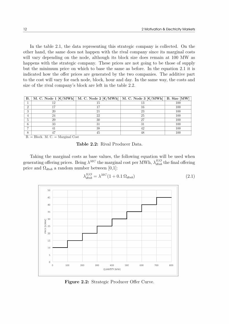
In the table 2.1, the data representing this strategic company is collected. On theother hand, the same does not happen with the rival company since its marginal costswill vary depending on the node, although its block size does remain at 100 MW ashappens with the strategic company. These prices are not going to be those of supplybut the minimum price on which to base the same as before. In the equation 2.1 it isindicated how the offer prices are generated by the two companies. The additive partto the cost will vary for each node, block, hour and day. In the same way, the costs andsize of the rival company’s block are left in the table 2.2.
B. M. C. Node 1 [€/MWh] M. C. Node 2 [€/MWh] M. C. Node 3 [€/MWh] B. Size [MW]1 12 15 13 1002 17 17 16 1003 20 21 23 1004 24 22 25 1005 29 30 27 1006 33 31 31 1007 41 38 42 1008 47 45 48 100
B. = Block. M. C. = Marginal Cost
Table 2.2: Rival Producer Data.
Taking the marginal costs as base values, the following equation will be used whengenerating offering prices. Being λMC the marginal cost per MWh, λ
S/Odtnb the final offering
price and Ωdtnb a random number between [0,1]:
λS/Odtnb = λMC(1 + 0.1 Ωdtnb) (2.1)
Figure 2.2: Strategic Producer Offer Curve.

2.2 The Electricity Market 13
The production of the companies are subdivided into 8 energy blocks in both cases.This way of presenting offers is very common in today’s electricity markets because itfacilitates the versatility in the combinatorial when creating a strategy and thus maxi-mize profits. As blocks are accepted, the marginal price increases in both cases. Thisorder of ascending prices can be seen more graphically in the figure 2.2 for the strategiccompany and in the figure 2.3 for the rival company.
Figure 2.3: Rivals Producer Offer Curves.
In addition to these aspects related to generators, ramping constraints are also takeninto account, which will be limited to 1000 MW/h in both directions when increasing anda decreasing the production. The blocks will be used to limit the maximum production,therefore P Gmax
nb = P Omaxnb = 100 MW due to all supply blocks are equal. The initial
value of production will be null: P Gininb = P Oini
nb = 0 MW, data to be taken into accountfor the ramping in the first simulation period of every day because they are differentauctions.
2.2.3.4 DemandSince the inverse problem deals with the demand in an elastic way, it is presented byblocks together with the associated prices as occurs in the generating companies. Incases where is desired to treat the demand as a single value, a simple calculation byadding the resulting accepted blocks is done and together with the energy offered themarket is cleared and thus it is obtained the market price. As shown in the table 2.3, the

14 2 Motivation & Electricity Markets
blocks are no longer all equal being the last four a half of the rest in terms of size. Al-though having two more blocks of demand (10 in total), if compared with the number ofblocks by the generators, the final computation of energy supply and demand per actoris the same. In addition to the table, its curves have also been illustrated in the figure 2.4.
Block Price [€/MW] Block size (N1&N2) [MW] Block size (N3) [MW]1 50 100 4002 45 100 4003 42 100 4004 40 100 4005 35 100 4006 30 100 4007 25 50 2008 20 50 2009 15 50 20010 10 50 200
N = Node
Table 2.3: Demand Data.
Figure 2.4: Demand Bidding Curves.
It is well known that demand varies according to the time of day, the day of the weekand the month of the year. The same energy is not consumed at 2 a.m. that at 13 p.m.and activity in both households and industries is different on a Tuesday compared toa Sunday, for instance. Due to these changes, the electricity tariff also varies in price
2.2 The Electricity Market 15
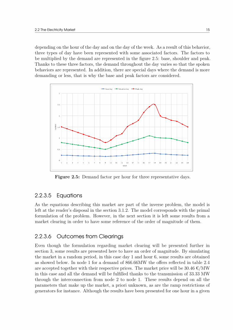
depending on the hour of the day and on the day of the week. As a result of this behavior,three types of day have been represented with some associated factors. The factors tobe multiplied by the demand are represented in the figure 2.5: base, shoulder and peak.Thanks to these three factors, the demand throughout the day varies so that the spokenbehaviors are represented. In addition, there are special days where the demand is moredemanding or less, that is why the base and peak factors are considered.
Figure 2.5: Demand factor per hour for three representative days.
2.2.3.5 EquationsAs the equations describing this market are part of the inverse problem, the model isleft at the reader’s disposal in the section 3.1.2. The model corresponds with the primalformulation of the problem. However, in the next section it is left some results from amarket clearing in order to have some reference of the order of magnitude of them.
2.2.3.6 Outcomes from ClearingsEven though the formulation regarding market clearing will be presented further insection 3, some results are presented here to have an order of magnitude. By simulatingthe market in a random period, in this case day 1 and hour 6, some results are obtainedas showed below. In node 1 for a demand of 866.66MW the offers reflected in table 2.4are accepted together with their respective prices. The market price will be 30.46 €/MWin this case and all the demand will be fulfilled thanks to the transmission of 33.33 MWthrough the interconnection from node 2 to node 1. These results depend on all theparameters that make up the market, a priori unknown, as are the ramp restrictions ofgenerators for instance. Although the results have been presented for one hour in a given

16 2 Motivation & Electricity Markets
node, this market will be simulated for the 30 days that make up a month resulting inseveral circumstances when applying alternative 1.
Block Strategic’s A. P. [MW] S. Off. Price [€/MW] Rival’s A. P. [MW] R. Off. Price [€/MW]1 100 10,401 100 12,9012 100 15,168 100 18,2143 100 20,592 100 21,7494 100 26,476 100 25,9835 33,333 30,463 100 29,7906 0 36,575 0 36,0057 0 41,174 0 41,6878 0 48,951 0 48,055
A.P. = Accepted Production; S. Off. Price = Strategic Offering Price; R. Off. Price = Rival Offering Price
Table 2.4: Market Outcomes in Node 1 for day 1 and hour 6.
2.2.4 1-Node Electricity Market2.2.4.1 Layout of the MarketOn account of the analysis that is to be applied in this project implies a single market,it is decided to reduce the previous market to a single node by eliminating their respec-tive connections and varying their components just a little. A market consisting of 9generating companies with a single demand is proposed, as shown in the figure 2.6.
Figure 2.6: 1-Node Electricity Market Overall.
Currently, not all generating companies have an associated marginal cost since theirproduction depends on a natural resource such as it is solar radiation, wind or even tidesamong others. As a consequence, it is considered convenient to introduce to the market awind farm with 100 % clean production which will represent all the production methodswhich have a lack of production cost. This leads to a more realistic supply curve wherethe first stretch of the curve will be formed by offers at cost 0 and therefore the staggering

2.2 The Electricity Market 17
will begin shifted to the right resulting in lower prices compared to the previous nodes.Figure 2.7 shows a market clearing indicating how the renewable energies are integratedin the forenamed curve. It will be showed later in section 3.1.2, the figure 3.1 where willbe presented the case that zero-cost generators are not taken into account and thereforethe price is higher if it is compared.
Figure 2.7: Market Clearing for the 1-Node Electricity Market.
2.2.4.2 Generating CompaniesAs mentioned in the previous section, wind power (W) represents the renewable partof production. On the other hand, each of the remaining 8 generators will representdifferent production methods such as nuclear, hydroelectric or gas, among others. Thereare also changes in the way of offering the energy since it has been considered that thereis no more than one block per company. In the end, the inclusion of blocks per generatorcan be considered as entering more generators in the market. That is why companiesare presented instead of blocks and, moreover, since the objective is to reveal prices, itis considered irrelevant for a didactic application to distinguish a company from a blocksince in the end a revealed price will be associated with an offer. Table 2.5 collects thedata formulated in the two following points where are described the generation groups:
• Wind Power Company (W): By having a completely renewable production, itsmarginal cost will be set at zero and therefore it will offer at zero cost its producedenergy in the market. As the nominal production capacity of wind turbines is smallcompared with traditional methods of energy generation, such as a nuclear or coalpower plant, 8 blocks of 30 MW will be established, thus being an integration ofaround 25% of renewable energies in the market. This parameter can be changeddepending on the real characteristics of the real market. This Wind Power com-pany will represent the total amount of free-cost energy production as it is only

18 2 Motivation & Electricity Markets
remarkable how is the price pushed in relation with the total renewable energyblock. Moreover, it is possible to collect the renewable production of Denmarkfrom public data so this would be a known parameter in a real application.
• Non-Renewable Companies (C1-C8): Together with the Wind Power Generator,eight more non-renewable generators will be found in order to have marginal costswhen producing. These companies will be able to offer one block each of whichwill be of 100 MW. The marginal costs of the blocks will be ascending in all thecompanies although their prices will be different if a given block is compared. Withthis, it is achieved variety in the offerings and also each company will representa method of generating energy. In order to create competitiveness apart fromobtaining different market clearings in each of the simulations, to the marginalcosts will be added an amount which will represent the profit of each electricitycompany. It will be assumed that, when a block is available, it will be fully offered,what is known in the electrical market as an all-in, and its starting price will bebounded between the marginal cost and a maximum of five more added euros. Thatis, if the block of Company C1 has a marginal cost of 10€, then its offering pricewill oscillate randomly in each time frame between 10 € and 15 €. Overlappingin the offers is achieved and therefore some variety in the market clearing results.With this, it is assumed to be a little closer to the reality of the market behaviour.Finally, the added part to the marginal cost is considerable when compared withthe 3-Node Market and therefore is more difficult to reveal its price due to itsspectrum. In equation 2.2 it is left how these prices are generated.
Number of blocks Block size [MW] M. C. [e/MW] Offering Price [e/MW]Wind Power (W) 8 30 0 0Company C1 1 100 10 10-15Company C2 1 100 15 15-20Company C3 1 100 20 20-25Company C4 1 100 25 25-30Company C5 1 100 30 30-35Company C6 1 100 35 35-40Company C7 1 100 40 40-45Company C8 1 100 45 45-50M.C. = Marginal Cost
Table 2.5: Market Data.
Again, taking the marginal cost as base values, the following equation will be usedwhen generating offering prices.Being λMC the marginal cost per MWh, λG
dtnb the finaloffering price and Ωdtnb a random number between [0,1]:
λGdtnb = λMC + (5 Ωdtnb) (2.2)

2.2 The Electricity Market 19
2.2.4.3 Other specifications of the MarketThe fundamental part of the changes in the supply part between the two markets arereflected in the previous section. As for the demand taking as reference the curve of node1 and the indices of the three representative days, data is generated for a whole year.Because bid prices sweep a greater range of values, there is a high variability of resultswhen market clearing is done. For the resolution of the market, the same equations willbe used as in the previous market with some caveats:
• The demand is treated in a non-elastic way: the values of each block that entersthe market will be taken and multiplied by the corresponding factor depending onthe type of day. Once said calculation is made, the final result of each block isadded and the demand is treated as a single value.
• As there are no nodes, there are no interconnections and therefore there are nocapacity restrictions of the transmission lines. There is also no reference node andtherefore it is not relevant to force the only node to be the slack bus.
• Since the calculated demand is presented as a single value and also does not havenodes, the equations that describe the market will vary with respect to the formu-lation of 1-Node Market. These equations are described in the following section.

20

CHAPTER 3Methods
Many applications could be considered when getting hidden data from a model givenavailable information. The reviewed literature is an example of how by means of a cor-rect formulation which reflects some behaviour, this exercise can be attained.
By cause of its simplicity and authenticity, the first part of this project will be areproduction and an analysis carried out in [8]. In this section the Inverse Optimizationequations are presented and explained. Together with the algorithm, the formulation ofthe model, which is a market clearing, is also exposed.
Finally, as an alternative to the previous method, the Ensemble Kalman Filter isexplained taking as reference the Simple Kalman Filter. In this last section all steps areanalyzed and come along with graphs and representations.
3.1 Inverse Optimization Problem
3.1.1 IntroductionSince the late 1980s, the Inverse Problem has been an object of research in variousfields of science. Its application in recent years has been focused more on geophysics,medical imaging or even on traffic balance problems, although other applications of thealgorithm are found in other fields such as engineering. Actually, in order to applyan inverse optimization problem, a physical system is required which must be modeledand which also may produce observable values. This type of problem is described as aforward problem because it identifies the values of the observable parameters given thevalues of the parameters of the model or, in other words, infers in the values of the modelparameters given the values of the observed parameters or optimal decision variables [12].
For the presented application in this section, as applied in [8], the model will bean electrical market through which values of the observed parameters will be obtainedand will be the results of the market clearing. Therefore, the appointed model will beconstituted by a series of equations representing a market clearing, bearing in mind thatthe same results could be obtained by applying an optimization problem of the economicdispatch type as it is done in [13].

22 3 Methods
It will be considered a strategic producer that offers electricity in a given market,taking into account that all the parameters related to the named producer are knownas a reference company is needed to make a strategy with respect to some competitors.As a priori information, aspects of the network will also be taken into account, such asthe technical parameters regarding the interconnection between nodes. Although thisinformation is generally not directly available from the strategic producer, for the appli-cation of the problem the marginal production costs of each of the competitors’ supplyblocks will be used. On the other hand, accepted blocks of generation and demand aftereach market clearing will be also considered as available data.
Therefore, through this application of the Inverse Optimization Problem, it will bepossible to reveal bid prices of competitors that in some of the study periods have beenmarginal and that, as a consequence, have also had an impact on the results of themarket clearing such are prices in each node and both production and demand acceptedblocks.
In the following section, the equations of the model to be treated and the subsequentapplication of the Optimization problem will be presented.
3.1.2 Market Clearing ModelAs has been well presented previously, the model to which the parameters are to beinferred is a market clearing. The notation of the problem is left for the reader’s knowl-edge in the chapter symbols. As a clarifying note regarding the symbols used in thissection, if a parameter depends on variables and then in the formulation they are notfound, it is because their value depends on these forgotten variables. In addition, in onecase it will be had a variable that will also behave as a parameter: this will be explainedthroughout the formulation.
Finally, and before presenting the model, contrary to what is proposed in [12], KKTconditions will not be applied to obtain results. Taking advantage of the fact that themodel is linear, the strong theorem of duality will be applied resulting in satisfactoryresults.
3.1.2.1 Primal Problem FormulationConsidering a market of the pool type, which has a very similar behavior in the differentmarkets of both Europe and the USA, the following linear problem is presented whichwill seek to maximize the social welfare of the forenamed market. For this purpose, itwill be needed an offer and a demand. On the supply side, a set of strategic and rivalproducers are considered, which will offer different amounts of energy represented by
3.1 Inverse Optimization Problem 23
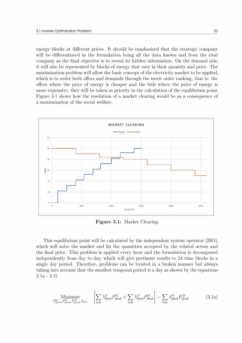
energy blocks at different prices. It should be emphasized that the strategic companywill be differentiated in the formulation being all the data known and from the rivalcompany as the final objective is to reveal its hidden information. On the demand side,it will also be represented by blocks of energy that vary in their quantity and price. Themaximization problem will allow the basic concept of the electricity market to be applied,which is to order both offers and demands through the merit order ranking, that is: theoffers where the price of energy is cheaper and the bids where the price of energy ismore expensive, they will be taken as priority in the calculation of the equilibrium point.Figure 3.1 shows how the resolution of a market clearing would be as a consequence ofa maximization of the social welfare.
Figure 3.1: Market Clearing.
This equilibrium point will be calculated by the independent system operator (ISO),which will solve the market and fix the quantities accepted by the related actors andthe final price. This problem is applied every hour and the formulation is decomposedindependently from day to day, which will give pertinent results to 24 time blocks in asingle day period. Therefore, problems can be treated in a broken manner but alwaystaking into account that the smallest temporal period is a day as shown by the equations3.1a - 3.1l.
MinimizeP G
dtnb,P O
dtnb,P D
dtnk,δdtn
[∑tnb
λGdtnbP
Gdtnb +
∑tnb
λOdtnbP
Odtnb
]−
∑tnk
λDdtnkP D
dtnk (3.1a)

24 3 Methods
subject to:[∑b
P Gdtnb +
∑b
P Odtnb
]−
∑k
P Ddtnk =
∑n
Bnm(δdtn − δdtm) : λdtn ∀t, n, b ∈ Θn (3.1b)
0 ≤ P Gdtnb ≤ P Gmax
nb : µGmindtnb , µGmax
dtnb ∀t, n, b (3.1c)
0 ≤ P Odtnb ≤ P Omax
nb : µOmindtnb , µOmax
dtnb ∀t, n, b (3.1d)
0 ≤ P Ddtnk ≤ P Dmax
dtnk : µDmindtnk , µDmax
dtnk ∀t, n, k (3.1e)
− RGdwnn ≤
∑b
P Gd1nb −
∑b
P Ginidn ≤ RGup
n : µGdwnd1n , µGup
d1n ∀n (3.1f)
− RGdwnn ≤
∑b
P Gdtnb −
∑b
P Gd(t−1)nb ≤ RGup
n : µGdwndtn , µGup
dtn ∀t > 1, n (3.1g)
− ROdwnn ≤
∑b
P Od1nb −
∑b
P Oinidn ≤ ROup
n : µOdwnd1n , µOup
d1n ∀n (3.1h)
− ROdwnn ≤
∑b
P Odtnb −
∑b
P Od(t−1)nb ≤ ROup
n : µOdwndtn , µOup
dtn ∀t > 1, n (3.1i)
Bnm(δdtn − δdtm) ≤ P maxnm : νmax
dtnm ∀t, n, m ∈ Θn (3.1j)
− π ≤ δdtn ≤ π : ξmindtn , ξmax
dtn ∀t, n (3.1k)
δdtn = 0 : ξ1dt ∀t, n = 1 (3.1l)
The equation to optimize (1a) is the minus social welfare which is the differencebetween supply and demand. Instead of maximizing the left region a minimizing problemis applied to its right one. The network is represented through a dc linear model, and thepower balance at every node is enforced by equation (1b). This means that if there is asurplus when producing or demanding there will be a difference and will result in a powerflow through the transmission line between nodes that must respect the saturation limitsimposed by the technical aspects in the interconnections. Equations (1c-1e) representthe generation limits of each of the companies, which will be equal to the size of the blockthat corresponds to them. Indeed, this constraint controls the block size depending onthe actor. Equations (1f-1i) define the ramp time restrictions between the initial periodand the first period as well as between periods for both the generators and the demands.This constraint deals with generators technical limitations which are considered to beknown in this model. Equation (1j) fixes the interconnection in order to not overload thelimit capacity of the line. Constraint (1k) indicates that the phase angle of the voltagesin each node will be between 180º and -180º and constraint (1l) fixes the angle of thevoltage in node 1 to 0 so that we have the bus as a reference and so the rest of anglestake values with respect to mentioned bus.

3.1 Inverse Optimization Problem 25
3.1.2.2 Dual Problem FormulationAs can be seen in the previous formulation, each restriction is related to a dual variable.This is because this inverse optimization problem will use the strong duality theorem asa constraint instead of KKT (Karush-Kuhn-Tucker) conditions. It is recalled that thestrong duality theorem ensures that if a Linear Programming (Primal) problem has anoptimal solution, then the corresponding Dual problem also has an optimal solution, andtheir respective values in the objective function are identical. Taking this into account,the dual formulation of the previous market clearing is left:
MaximizeΞd
−∑tnb
P Gmaxnb µGmax
dtnb −∑tnb
P Omaxnb µOmax
dtnb −∑tnk
P Dmaxdtnk µDmax
dtnk +∑
n
µGdwnd1n (P Gini
dn − RGdwnn )
−∑
t>1,n
µGdwndtn RGdwn
n −∑
n
µGupd1n (RGup
n +P Ginidn )−
∑t>1,n
µGupdtn RGup
n +∑
n
µOdwnd1n (P Oini
dn −ROdwnn )
−∑
t>1,n
µOdwndtn ROdwn
n −∑
n
µOupd1n (ROup
n + P Oinidn ) −
∑t>1,n
µOupdtn ROup
n −∑tnm
P maxnm νmax
dtnm
−∑tn
πξmindtn −
∑tn
πξmaxdtn (3.2a)
subject to:
λdtn −λGdtnb +µGmin
dtnb −µGmaxdtnb +µGdwn
dtn −µGdwnd(t+1)n −µGup
dtn +µGupd(t+1)n = 0 ∀t < T, n, b (3.2b)
λdtn − λGdtnb + µGmin
dtnb − µGmaxdtnb + µGdwn
dtn − µGupdtn = 0 t = T ∀n, b (3.2c)
λdtn −λOdtnb +µOmin
dtnb −µOmaxdtnb +µOdwn
dtn −µOdwnd(t+1)n −µOup
dtn +µOupd(t+1)n = 0 ∀t < T, n, b (3.2d)
λdtn − λOdtnb + µOmin
dtnb − µOmaxdtnb + µOdwn
dtn − µOupdtn = 0 t = T ∀n, b (3.2e)
− λdtn + λDdtnk + µDmin
dtnk − µDmaxdtnk = 0 ∀t, n, k (3.2f)∑
m
Bnm(λdtm −λdtn)+∑m
Bnm(νmaxdtmn −νmax
dtnm)+ξmindtn −ξmax
dtn +(ξ1dt)n=1 = 0 ∀t, n (3.2g)
µGmindtnb , µGmax
dtnb , µOmindtnb , µOmax
dtnb , µDmindtnb , µDmax
dtnb , µGdwndtn , µGup
dtn , µOdwndtn , µOup
dtn , νmaxdtmn,
ξmindtn , ξmax
dtn , ξ1dt > 0 ∀t, n, b, k (3.2h)
where:
Ξd =λdtn, µGmin
dtnb , µGmaxdtnb , µOmin
dtnb , µOmaxdtnb , µDmin
dtnb , µDmaxdtnb , µGdwn
dtn , µGupdtn , µOdwn
dtn , µOupdtn ,
νmaxdtmn, ξmin
dtn , ξmaxdtn , ξ1
dt
are the dual variables.
26 3 Methods
Remark that, contrary to the inverse problems which use as a model a unit commit-ment optimization problem, this market clearing has the advantage of not consideringdiscrete decisions variables. Taking this into consideration, the formulation becomeslinear and thus not convex, helping to derive its associated dual problem. Moreover, itwill be required less computation running time if compared and it could be said thatit reflects fairly how the current European markets behave from an external point of view.
Both problems primal and dual will be used in the following section when formulatingthe inverse optimization problem.
3.1.3 Inverse Problem FormulationFor the resolution of the Inverse Problem, a prior market clearing must be carried out, inorder to obtain data such as the accepted production of the strategic producer and thatof each rival, as well as the accepted demand blocks and the market clearing price ineach node. Once this data set is obtained, it is proceeded to the first version formulationof the Inverse Problem:
MinimizeΛ
∑tnb
|λOdtnb − λOini
dtnb | (3.3a)
subject to:(3.1a) = (3.2a) ∀d (3.3b)
(3.2b) − (3.2h) ∀d (3.3c)
where:
Λ =λO
dtnb, µGmindtnb , µGmax
dtnb , µOmindtnb , µOmax
dtnb , µDmindtnb , µDmax
dtnb , µGdwndtn , µGup
dtn , µOdwndtn , µOup
dtn ,
νmaxdtmn, ξmin
dtn , ξmaxdtn , ξ1
dt
are the variables of the above problem.
The main objective of the previous optimization problem is to bring as close as pos-sible the different values of offer prices to an initial estimate given for each price. Notethat the initial estimate will change throughout simulations. Restriction (3.3b), as dis-cussed above, applies the strong theorem of duality by forcing the solution vector ofthe objective function of the primal problem to be equal to the solution vector of theobjective function of the dual problem. In addition, and previously solving the problem(3.3a), it has been necessary to make use of solutions of the market clearing problem andthus the restrictions of the primal problem are not necessary to constraint the problemof inverse optimization.
Once the inverse problem has been raised, the last qualification in relation to theformulation must be clarified. The problem must be linearized in order to be able to
3.2 Ensemble Kalman Filter 27
apply a solver for a linear programming and in this sense reduce computation time. Bymeans of a simple linearization method, the following problem will be considered as thedefinitive one as exposed in [12]:
MinimizeΛ,αdtnb,βdtnb
∑dtnb
(αdtnb + βdtnb) (3.4a)
subject to:λO
dtnb − λOinidtnb = αdtnb − βdtnb ∀d, t, n, b (3.4b)
αdtnb, βdtnb ≤ 0 ∀d, t, n, b (3.4c)
(3.3b) − (3.3c). (3.4d)
The solution to the previous problem will be collected in the variable λ∗Odtnb, which will
indicate the offering price of each of our rivals depending on the calculation period andenergy block. Analyzing the formulation of the problem, it can be observed that whena supply price that is at the same time marginal in the market clearing and thereforegenerates a market price in a given node for a given period, the initial estimate madeλOini
dtnb will not influence the result. However, having initial estimates for each of the rivalblocks, when a price is not shown, it will be forced to have the optimal value equal toour assumption. Therefore, if there are offers of rivals which are not marginal, that is,if they are part of the accepted production and are always below the equilibrium pointwhatever the period, it will be forced to an initial estimate value without its value beingproven.
3.2 Ensemble Kalman Filter
3.2.1 IntroductionThe Ensemble Kalman Filter (EnKF) is a recursive filter which is used as a computa-tional technique in order to inference models composed by state variables that changein a given Euclidean space. This structure of space is presented within this techniquebecause for the representation of the different states of the variables it will be neededa vector gathering all the associated values (that correspond to a Probability DensityFunction) and will be represented in a given region of the mentioned space. As thereare recursive transitions within each time step, two dimensions of the Euclidean spacewill be used to get the final result given by the algorithm and will be used to advancethroughout the remaining dimension into the next application forward in time. Thisbehaviour could be arduous to follow without a graphic representation, for this reasonfigures will come along when exposing equations to clarify each evolution of the variables.
28 3 Methods
Unlike the simple Kalman Filter, the EnKF works with an ensemble of vectors ap-proximating a state distribution whatever its nature. In the following sections, it willbe seen that in order to make an estimation of a variable, its values must first maturealong a propagation and update of states following some model and observations. Thisrepresentation through ensembles allows a reduction of the dimensions due to the prop-agation of a small part of the ensemble instead of all the values if it is necessary, makinguse of the partial covariance matrix of the sample (called sample covariance). Whenthe initial guess of the state variable is propagated or updated, functions that representits behavior as a function of time are needed and, one of the advantages offered by thismethod is that it does not require a linear propagation function or a model composedby non-Gaussian distributions, besides that the degree of dimensionality of the variablesis not a hindrance when applying this method [14].
This filtering method has been used since the mid 90’s when Geir Evensen applied itto the field of geophysics. Since this period, it has had considerable repercussion withinthe scope of science due to its small formulation and its wide range of application. Aquite popular implementation is found in data assimilation processes for meteorologicalproblems, where it must be applied for large amounts of data obtaining good results interms of computational requirements when compared with other similar methods withmore sophisticated objectives [15]. Besides, other applications apart from data assimila-tion are found. Such one example regarding estimating parameters between known statesis suggested in [16] where atmospheric methane concentrations are calculated thanks toreliable observations from anthropogenic and biospheric sources. As commented, not allthe applications seek the same outcome. In [17], the EnKF is used to adjust a givenmodel by recalculating its previous parameters and perform what is known as historymatching. This work has more to do with model validation. Taking as reference theseexamples, it is identified different applications in several fields of studies that succeededsupporting the versatility when applying this algorithm. Further in the following section,the basic formulation respecting the Kalman Filter is stated as a starting point.
3.2.2 Basic formulation
3.2.2.1 Kalman FilterBefore introducing the EnKF equations, it is valuable to understand first how a SimpleKalman Filter (KF) works. Point that the mechanism of both the Ensemble and theSimple is the same, being the first used when the systems are high-dimensional and thecalculation of the covariance matrix is not computationally feasible. The KF is wideused in signal processing and assumes that all the state variables follow a Gaussian dis-tribution. Its equations are split in a prediction and a correction part, being inferredrecursively. This means that a process is estimated and then corrected by using a feed-back control thanks to some measurements [18]. In the following figure, it is describedhow the algorithm progress in each time step and which could serve as a reference for

3.2 Ensemble Kalman Filter 29
the later formulation.
Figure 3.2: The ongoing discrete Kalman Filter cycle.
In a first step, it is assumed that a distribution of the variable is hold which willbe called initial estimation of the state variable and will come from the previous timestep. If prior information is not available, initial values for its mean and variance areassociated without matter their magnitude. Therefore, it is had an initial information ofthe estate (xt−1, Pt−1) which will be used throughout a couple of expressions to calculatethe first guess of its new estate. For this purpose, it is required a model or a relation ofthe state between time steps. In equations 3.5 and 3.6 it is suggested to have a linearrelation represented by the Mt matrix. This constant will be used to propagate themean value and the covariance, resulting in xt and Pt. The prediction equations can beformulated as follows:
xt = Mt xt−1 (3.5)
Pt = Mt Pt−1 MTt + wt, wt ∼ Nn(0, Qt) (3.6a)
or
Pt = Mt Pt−1 MTt + Qt (3.6b)
Here, the resulting parameter is what is known as a priori estimation of the state vec-tor in the following time period t. As assumed before, there is a linearity between statesbut this relation will depend on how the state vector behaves along time. Furthermore,the value of Mt should vary in time if the model behaves dynamically. To the resultingcovariance, it is added a random error in this first estimation which will follow a normaldistribution with a null mean and some Qt standard deviation (also called white error)adding uncertainty to the resulted distribution. This can be graphically observed infigure 3.4.
As this first step is a prediction, it is required some measurement regarding theparameter to obtain an accurate final distribution as a result of an uncertainty reduction.

30 3 Methods
Accordingly, this measurement will infer in the a priori state estimate together with theKalman Gainer which will been obtained based on the relation between both values.Being yt an observation or measurement of the true state and assuming that there is arelationship between this observed value and the first estimation, the equation will be:
yt = Ht xt + vt, vt ∼ Nn(0, Rt) (3.7)
The matrix Ht will give a linear relationship between both variables along with an as-sociated error. Here is again assumed to have a proportional between variables althoughit will depend on the nature of the model. This added error will have the same attributesas the one in equation 3.6a, being both of them independent. As yt is an observationthat comes from a measurement, it is supposed that an error is committed when gettingthe value. As happens with Ht, the process noise covariance Qt, the measurement noisecovariance Rt and the Ht matrix will change over time steps, that is why their subscriptindicates a time dependence.
Once the observation is presented, it will serve by means of the Kalman Gainer (orblending factor) to correct the a priori state estimate represented by the results inequations 3.5 and 3.6. This constant will bring the mean of the first estimate towardsthe mean of the observation distribution as well as conceiving a reduction of the resultingfinal state estimate standard deviation. Assuming another time that an error will beassociated and that will be exactly the same held in the previous equation, its formulationwill be:
Kt = Pt HTt (Ht Pt HT
t + Rt)−1 (3.8)
This equation is considered to be the first one in the update step and its value willvary depending on how accurate is the a priori estimation. See that if the measurementnoise covariance remains null, then the optimal state estimate will be equal to the mea-surement. On the other hand, if the a priori covariance Pt yields to zero then the optimalstate estimate would be the same the a priori state estimate. Here are found the boundsbetween which the Kalman Gainer is correcting the final result. One last remark, whichcomes from the last statement, is that if the a priori estimate error covariance is consid-erable, the value of the gainer will be higher to reduce it (see their proportional relation).
Finally, with the gainer already calculated, the correction of both the covariance errorand mean value of the state estimate is achieved by applying the following equations:
xt = xt + Kt(yt − Ht xt) (3.9)
Pt = (I − Kt Ht) Pt (3.10)

3.2 Ensemble Kalman Filter 31
As this method is recursive, after each time step will be a new measurement andtherefore the process will be applied again following the presented equations. The nota-tion on the subscripts will vary as an indicator of a step forward.
As the equations describing this process require some graphical guidance to deeplyunderstand how the data flow is evolving along them, some figures are left below. Infigure 3.3 it can be seen both predictive and update state along with their correspondingequations. In addition, some representative Gaussian distributions are plotted in figure3.4 which will help to appreciate how the covariance errors are minimized. As appointedat the beginning of this section, the main application of this recursive filter is on signalprocessing as are the GPS systems. In this type of applications what is wanted, apartfrom an accurate result, is the reduction of the uncertainty that is already presented inthe a priori estimation. In figure 3.4, this predicted state estimation has a PDF thatfollows a normal distribution with a mean value of 7 and a standard deviation of 1.Depending on the application, the value of the standard deviation may be acceptableor not but always is a good exercise to reduce it as it means that the distribution haslower error covariance and thus more credibility. Then, assuming that the measurementrepresent a lower erratic value and thanks to the correction conducted by the effect of theKalman gainer, what results is an optimal state estimate with a lower error covarianceif compared with the initial predicted state estimate. Even if the uncertainty in yt islarger than the first predicted estimate which means that its associated R is large, thevalue of the Kalman gainer will absorb this particularity in each time step and the errorwill be mitigated along updates [19].
Figure 3.3: Steps in the KF cycle.

32 3 Methods
Figure 3.4: Optimal State Estimator Algorithm.
Some problems can come up depending on how the measured value is obtained. Inthese sample applications, it is supposed that a sensor takes some values about the po-sition however, some interpretation is required when the measurement is a single valuewith a null Rt. This type of drawback is presented when extrapolating this algorithm tothe purpose of this project and it will be analyzed properly. In any case, the EnsembleKalman Filter will be exposed firstly taking as reference the algorithm above.
3.2.2.2 The Ensemble Kalman FilterAs took place with the KF, the Ensemble Kalman Filter behaviour is also based on theBayesian update problem which uses the Bayes theorem. This implies that a PDF ofa posteriori state variable can be obtained from a priori PDF taking into account itslikelihood function. Bayesian update problem or Bayesian inference, calculates the aposteriori probability according to Bayes’ theorem:
P (A | B) = P (B | A) P (A)P (B)
(3.11)
It is also often said that the Ensemble Kalman Filter is a consequence of the KalmanFilter if considering Monte Carlo approximations which rely on random sampling toobtain numeric results. By analyzing the following formulation, it will be appraised thatboth Bayesian Inference and Monte Carlo approximation have influence on the algorithm[20]. On the part of Bayesian Inference, as seen in the previous section, it will be theobservation the distribution which will behave as the likelihood function to infer the pre-vious guess. Monte Carlo methods will be applied when desired to generate ensemblesfrom a given distribution. Thanks to this method, a simulation of results accounting forvariability of its factors or inputs will be reached. Setting aside this first introduction,
3.2 Ensemble Kalman Filter 33
in the following paragraphs the formulation of this algorithm is presented.
From this point, the Gaussian distributions for each state variable will be formedfrom numbers which are known as realizations and that, when gathered, compose anensemble. This means that the mean and variance of each PDF is no longer taken intoaccount to calculate shifted values neither error covariance matrices. Instead, matriceswill collect ensembles and the forecasting and update steps will be realized with themattaining to a great variability. Therefore, the initial state estimate will be constitutedby a matrix which its row’s dimension (n) will represent the number of individual initialstates estimate x
(i)t−1 and its column’s dimension (N) the number of samples gotten from
each state variable. For instance, if it is had four temperatures in four different locationswith a hundred samples for each one, the dimension of the matrix will be (4, 100). Afair representation could be the following:
xt−1 =
x11 x12 x13 . . . x1n
x21 x22 x23 . . . x2n
... ... ... . . . ...xN1 xN2 xN3 . . . xNn
t−1
(3.12a)
x(ij)t−1 ∼ Nn(µt−1, Σt−1), i = 1, 2, ..., N. j = 1, 2, ..., n. (3.12b)
The previous matrix will be named the initial state estimation ensemble. The valuesconforming the columns of the matrix are directly related with the distribution depictedin equation 3.12b and therefore, the covariance error it is implicit in the values and thatis the reason why only one equation is required. As it was proceeded with the KF, thea priori state estimation will be calculated by relating the presented ensembles with agiven relation matrix, Mt also in this case, and with some added error wt. The followingformulation reflects the relationship.
xt = Mt xt−1 + wt, wt ∼ Nn(0, Qt) (3.13a)x
(ij)t ∼ Nn(µt, Σt), i = 1, 2, ..., N. j = 1, 2, ..., n. (3.13b)
The resulting matrix will have the same dimensions as the initial guess matrix, there-fore the dimension of Mt must be (N, N). Moreover, this relation matrix is important inthe formulation as with its diagonal the individual propagation of the variables can becontrolled. However, what is more, thanks to its square dimension every state variablecan be correlated with each other when tuning properly the upper and lower trianglesof the matrix.
Continuing with the formulation, as this is a forecast that must be inferred consid-ering a measurement yt in each time step, an update based on this value will be carried

34 3 Methods
out. It is worthy to mention that two options are applicable when updating the firstpredicted ensemble: stochastically or deterministically. In this project, the updating willbe done in a stochastic point of view as it is more logical for the nature of the model. Tojustify this decision, some differences between them are exposed below. Furthermore atthe end of this section an example of the algorithm will be showed with a deterministicupdate to fully understand the main disadvantage.
When applying deterministic updates:
• There is no need of generating a simulated observation. The simulated observationis an initial guess of the measurement that will be corrected afterwards by the realone. This simulated parameter helps to control the shape of the final PDF which isvaluable in the case of this project. Moreover, the observations in the applicationwill not represent all the state variables collecting only one measurement per timestep. Therefore, this matrix will also complete the estimation of all the variableswithout really seeing them. In next chapter all this formulation features will beproperly explained.
• Before obtaining posterior draws of the state variable, it is required to apply twomore steps called standardize and ”unstandardize”. This additional part comes alsowith a Trochowski decomposition when computing results with large ensembles,leading this alternative to be computationally unfeasible when applying to a largenumber of time steps which is the case.
Following the stochastic update and taking into consideration the result of equation3.13a, the covariance sample matrix is calculated. Remind from the introduction partof this section that, the representation of the states by means of ensembles permitspropagation making use of the partial covariance matrix of the sample. Hence, allrealizations will be taken into account when reaching xt but not with the covariancematrix calculation as it is recommended an approximation which makes the algorithmCPU viable. From the a priori state estimation ensemble, the mean value of each columnis determined and thus conforming the matrix Et(x) as can be observed:
Et(xt) = 1N
N∑i=1
xij (3.14)
This matrix will contain the average value for each of the individual state variablerepresented in each column and its dimension will be (1, n). As it is desired to subtracteach related mean value to all the realizations that form an state ensemble, the resultedEt matrix will be resized to a (N, n) dimension as can be seen in equation 3.15 throughmultiplying in the left side by an eye matrix. Additionally in this equation, the men-tioned subtraction is done obtaining the At matrix that will be used to calculate thecovariance sample matrix St as can be seen in equation 3.16. Note that the values of
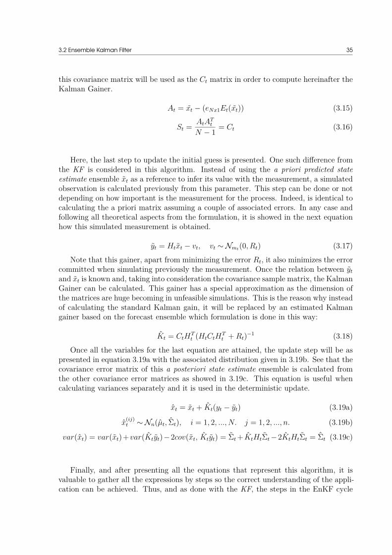
3.2 Ensemble Kalman Filter 35
this covariance matrix will be used as the Ct matrix in order to compute hereinafter theKalman Gainer.
At = xt − (eNx1Et(xt)) (3.15)
St = AtATt
N − 1= Ct (3.16)
Here, the last step to update the initial guess is presented. One such difference fromthe KF is considered in this algorithm. Instead of using the a priori predicted stateestimate ensemble xt as a reference to infer its value with the measurement, a simulatedobservation is calculated previously from this parameter. This step can be done or notdepending on how important is the measurement for the process. Indeed, is identical tocalculating the a priori matrix assuming a couple of associated errors. In any case andfollowing all theoretical aspects from the formulation, it is showed in the next equationhow this simulated measurement is obtained.
yt = Htxt − vt, vt ∼ Nmt(0, Rt) (3.17)
Note that this gainer, apart from minimizing the error Rt, it also minimizes the errorcommitted when simulating previously the measurement. Once the relation between yt
and xt is known and, taking into consideration the covariance sample matrix, the KalmanGainer can be calculated. This gainer has a special approximation as the dimension ofthe matrices are huge becoming in unfeasible simulations. This is the reason why insteadof calculating the standard Kalman gain, it will be replaced by an estimated Kalmangainer based on the forecast ensemble which formulation is done in this way:
Kt = CtHTt (HtCtH
Tt + Rt)−1 (3.18)
Once all the variables for the last equation are attained, the update step will be aspresented in equation 3.19a with the associated distribution given in 3.19b. See that thecovariance error matrix of this a posteriori state estimate ensemble is calculated fromthe other covariance error matrices as showed in 3.19c. This equation is useful whencalculating variances separately and it is used in the deterministic update.
xt = xt + Kt(yt − yt) (3.19a)
x(ij)t ∼ Nn(µt, Σt), i = 1, 2, ..., N. j = 1, 2, ..., n. (3.19b)
var(xt) = var(xt)+var(Ktyt)−2cov(xt, Ktyt) = Σt + KtHtΣt −2KtHtΣt = Σt (3.19c)
Finally, and after presenting all the equations that represent this algorithm, it isvaluable to gather all the expressions by steps so the correct understanding of the appli-cation can be achieved. Thus, and as done with the KF, the steps in the EnKF cycle
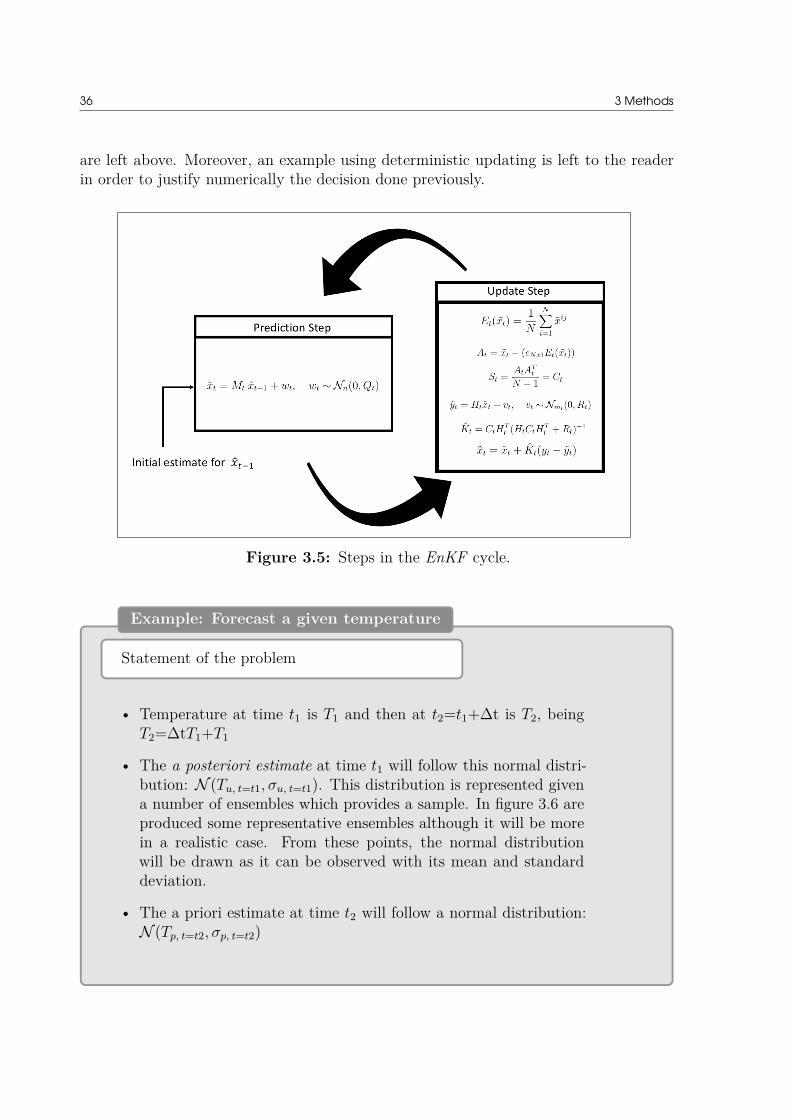
36 3 Methods
are left above. Moreover, an example using deterministic updating is left to the readerin order to justify numerically the decision done previously.
Figure 3.5: Steps in the EnKF cycle.
Example: Forecast a given temperature
Statement of the problem
• Temperature at time t1 is T1 and then at t2=t1+∆t is T2, beingT2=∆tT1+T1
• The a posteriori estimate at time t1 will follow this normal distri-bution: N (Tu, t=t1, σu, t=t1). This distribution is represented givena number of ensembles which provides a sample. In figure 3.6 areproduced some representative ensembles although it will be morein a realistic case. From these points, the normal distributionwill be drawn as it can be observed with its mean and standarddeviation.
• The a priori estimate at time t2 will follow a normal distribution:N (Tp, t=t2, σp, t=t2)
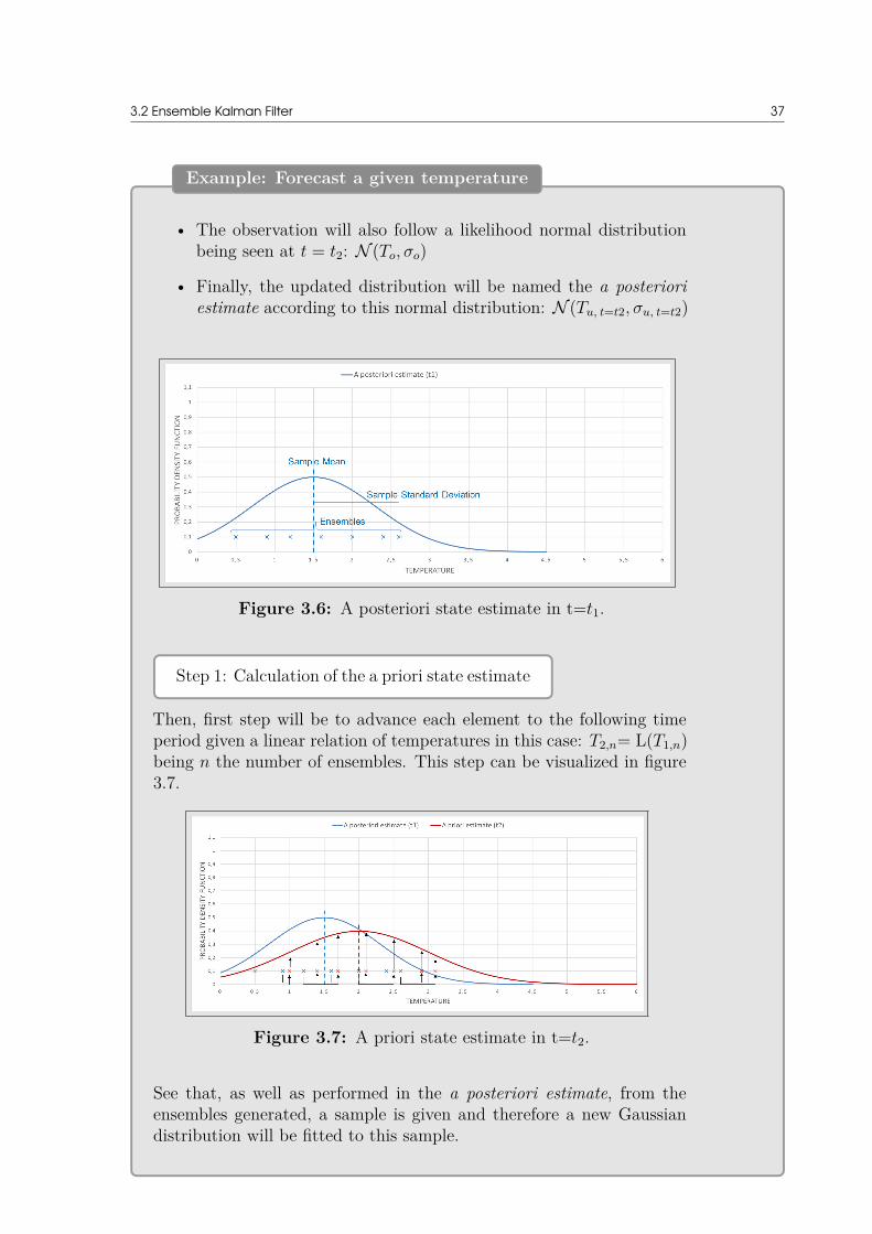
3.2 Ensemble Kalman Filter 37
Example: Forecast a given temperature
• The observation will also follow a likelihood normal distributionbeing seen at t = t2: N (To, σo)
• Finally, the updated distribution will be named the a posterioriestimate according to this normal distribution: N (Tu, t=t2, σu, t=t2)
Figure 3.6: A posteriori state estimate in t=t1.
Step 1: Calculation of the a priori state estimate
Then, first step will be to advance each element to the following timeperiod given a linear relation of temperatures in this case: T2,n= L(T1,n)being n the number of ensembles. This step can be visualized in figure3.7.
Figure 3.7: A priori state estimate in t=t2.
See that, as well as performed in the a posteriori estimate, from theensembles generated, a sample is given and therefore a new Gaussiandistribution will be fitted to this sample.
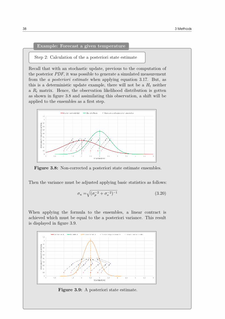
38 3 Methods
Example: Forecast a given temperature
Step 2: Calculation of the a posteriori state estimate
Recall that with an stochastic update, previous to the computation ofthe posterior PDF, it was possible to generate a simulated measurementfrom the a posteriori estimate when applying equation 3.17. But, asthis is a deterministic update example, there will not be a Ht neithera Rt matrix. Hence, the observation likelihood distribution is gottenas shown in figure 3.8 and assimilating this observation, a shift will beapplied to the ensembles as a first step.
Figure 3.8: Non-corrected a posteriori state estimate ensembles.
Then the variance must be adjusted applying basic statistics as follows:
σu =√
(σ−2p + σ−2
o )−1 (3.20)
When applying the formula to the ensembles, a linear contract isachieved which must be equal to the a posteriori variance. This resultis displayed in figure 3.9.
Figure 3.9: A posteriori state estimate.

3.2 Ensemble Kalman Filter 39
Example: Forecast a given temperature
Comments and conclusions
Better results must be obtained if a stochastic update is applied.Instead of separating mean and variances from the sample, equationsare applied directly to each ensemble. Much more relations are donebetween single values and consequently a greater collection of results isobtained from which a PDF is possible to be drawn. When applyingthe equations from this point of view, there is no need of applyingequation 3.20 and less computation time is required.
This example updates in a deterministic way with a ”standardize-unstandardize” calculation perspective, and it is solved according tothis alternative to show that if compared with the stochastic update isworthless when relieving the scope of this project. The relation betweenensembles in the model presented in last section is not linear and thusthe contraction done in the last part of this example becomes reallyarduous.
Moreover, the simulated observation is not presented in the determinis-tic update and will be a key parameter in the strategy proposed furtherin this document.
3.2.3 Implementation for revealing pricesAs commented in the prior sections, this algorithm is versatile and if tuned properly canbe applied to different purposes. Moreover, the case of study when revealing prices isnovel and therefore some of the variables must be treated in the best way, accordingto their attributes to acquire logical results. One such example are the observations, incompliance with the formulation an error is added to the value assuming a disturbancein the measurement sensor. But what if the nature of the observation is discrete and100% correct as it can be a market price? This will be studied in the following sectioncomparing results when simulating under different assumptions.
Another issue which has to do with the formulation is the propagation of the ensem-bles. It is clear that computation becomes easy in case of calculating estimated statevariables shifting means and updating variances. Nevertheless, a great order of magni-tude is advisable when generating realizations and this is achieved by relating all therealizations of the ensembles.

40 3 Methods
These two issues will be taken into consideration regarding the formulation. Alongnext chapter, all changes or assumptions made will be explained.

CHAPTER 4Results
Once the methodology is presented, the results obtained will be shown. In the case ofthe Inverse Optimization Problem, a simple equation that will serve as a filter to obtainmarginal costs will be presented prior to the results. In the case of the Ensemble KalmanFilter, some steps prior to the methodology will be carried out in order to have an initialstate of the variables. Once exposed, the algorithm will be applied to three differentcases. Because the current application of this method varies from the one applied in thisproject, it requires special treatment to some parameters to obtain results. Since this ispart of the strategy adopted, it has been considered appropriate to separate additionalequations from classical formulation: if the equations exposed in section 3 change, saidchanges will be explained.
4.1 Inverse OptimizationIn this section, the results obtained from the first methodology are exposed. The InverseOptimization is applied to the 3-Node Market and therefore prices from three rivalcompetitors, one per node, are analyzed by means of tables and graphs. Furthermore,at the end of this section, some conclusions will be drawn from the outcomes.
4.1.1 Revealing marginal costsWhen the formulation is applied, a set of prices per block, node and producer is ap-proached. These prices that each company offers, will be equal or higher to their marginalcost as financial losses when producing want to be averted. As a consequence, and takingas inputs these sets of outcoming prices, the following equation will be used for eachrival’s block in all three nodes when estimating marginal costs.
ˆλOtruenb = Min
∀d,t
λ∗O
dtnb
∀n, b (4.1)
Hence, this equation will yield to the minimum price given all the associated valuesof a an energy block during all the simulation period which, in this case, is 30 days.
The assumption of offering always above the marginal price is not a certain represen-tation of what really happens in real markets as this value could be lower to guaranteethat an energy block is fully accepted, for instance. Nevertheless, as the model is con-trolled and determines the offering values to be always greater, this is not a problem

42 4 Results
when solving. Anyhow, a parallel solution to this issue could be employed if happenscalculating the average offered price instead.
Taking into consideration the data provided in section 2 regarding the electricitymarket model and the formulation left in section 3, the linear inverse problem is applied.Once rival producers’ offer curves λ∗O
dtnb are sifted by equation 4.1, the rival produc-ers’marginal costs curves ˆλOtrue
nb per block and node are obtained. These results aregathered in table 4.1 as can be identified below.
b 1 2 3 4 5 6 7 8λOtrue
1b 12,000 17,000 20,000 24,000 29,000 33,000 41,000 47,000ˆλOtrue
1b - 17,022 20,122 24,030 29,039 33,051 - -ˆλOmax
1b - 18,486 21,964 26,361 31,789 36,093 - -λOtrue
2b 15,000 17,000 21,000 22,000 30,000 31,000 38,000 45,000ˆλOtrue
2b 15,219 17,016 21,040 22,004 30,064 31,056 - -ˆλOmax
2b 16,497 18,491 23,082 24,105 32,838 33,993 - -λOtrue
3b 13,000 16,000 23,000 25,000 27,000 31,000 42,000 48,000ˆλOtrue
3b - 16,330 23,012 25,005 27,006 - - -ˆλOmax
3b - 17,186 25,281 27,44 29,284 - - -
Table 4.1: Estimated and True Marginal Costs in [€/MWh].
The results of the table are split into three graphical plots representing clearings in allthree nodes taking into account all technical aspects from producers and also technicalaspects from the grid. These are left below in figures 4.1, 4.2 and 4.3.
Figure 4.1: Estimated Marginal Costs: Node 1.

4.1 Inverse Optimization 43
Figure 4.2: Estimated Marginal Costs: Node 2.
Figure 4.3: Estimated Marginal Costs: Node 3.
All the estimated marginal costs are compared with their associated real value toverify whether the result is accurate or not. This real values come from the previousinformation that it is had from competitors and used as an input in the market clearingoptimization problem. Moreover, the maximum value of each block is also referenced sothe spreading of the prices along 30 day can be observed.
The ramping constraints for the generation and demand sides together with the in-terconnection power limits, produce that not all the prices have been marginal. This
44 4 Results
results in hidden information which is never reached and thus can not be represented asa part of the final solution even though it is had knowledge of their true values. Somehidden prices have more importance than others from a strategic point of view. The caseof not reveling the lower blocks’ price could not be a problem due to, with those prices, isdifficult to employ market power and push competitors close to the market price beyondthe clearing point. The simulation has been extended to a longer time period withoutimproving the number of revealed prices, concluding that the restrictions are the causers.
Analyzing all numerical results of the table 4.1, it can be observed that the estimatedmarginal cost of the prices that at least once have been a market price (or marginal) andthus had set the corresponding LMP in a given node, are close to their real values. Thelogic of taking the minimum number indicates a properly functionality when estimatingthe marginal costs as they are the base number to generate offerings.
Once the outcomes from the optimization problem are discussed, some conclusionsare going to be exposed. Being critical and taking into account the scope of this project,some aspects will be considered as decisive contributions and other will be stated aschallenges to be covered by the following methodology.
4.1.2 ConclusionsThis first methodology has positive features when applying to a given market. The for-mulation is simple since the optimization problem takes as reference the market clearingproblem used in the proposed model. Moreover, the linearization becomes elegant beingthe strong duality theorem applied successfully in the constraints. This results in lowsimulation time as it is not computationally demanding if compared with other alterna-tives that apply an optimization approach.
On the other hand, some aspects that can been improved to achieve the offeringprices are also encountered. Many are found and, for that reason, a list is presented:
• First, some prices are not marginal at any simulation period and therefore they areleft as unknown variables though they could be estimated by a simple polynomialregression, for instance. Being analytic, it is appropriate as there exist some pricesthat are allocated in the lower part of the offering curve and thus will not becomein a threat from a strategy scope. Despite this, estimating prices from competitorsthat are not in any market clearing should be a positive study. If obtained, higherprices beyond the equilibrium point will be known and will result in the limitedoffering price when executing power market.
• Another issue is encountered regarding all the required data in order to apply thismethodology. Both accepted offering and demanding blocks, block size, initialproduction level for each day or even ramping constraints, between others inputs,

4.2 Ensemble Kalman Filter 45
are required to carry out the proposed formulation. The problem with this amountof information is that, probably is not going to be accessible to a company as itwill be considered a strategic advantage given from a competitor as well as havingaccess to private information from the market TSO. One such proposal could beto simplify the market in terms of required information but generating a faithfulsupply and demand curve which give prices according to the real studied market.
• Finally, the last drawback presented is that, in the end, the offering prices are notcalculated but used further on. Marginal prices are revealed instead of offeringprices. Indeed, these offering prices are used as a whole gathered by blocks todetermine their minimum value and thus obtain the associated marginal cost.
The scope of this project wants to go one step forward. Alternately of using hiddendata in the algorithm, only market prices will be taken into account as inputs. This is,from public prices, revealing hidden parameters inside a model as are the offering prices.It is clear that technical data regarding generating companies is needed but only forthe model to get market outputs. This will only deal with constructing accurate curveswhen compared with a real world market. One consequence when facing a problem withmultiple hidden variables that are calculated only when one is observable is that, someassumptions will be implied within some logical range. One such example could be toassign to the energy blocks a quantity small enough to detect a change in the price whenmarket clears. All the assumptions will be explained in the following section where thesecond alternative is applied.
4.2 Ensemble Kalman FilterIn this section, it will be suggested the second alternative taking as reference the secondmethodology exposed in section 3. Gaussian distributions will come up when represent-ing prices instead of discrete values. Moreover, with this second option, apart fromreaching hidden variables, it is wanted to offer remedies to the weak points presented inthe conclusions of the previous approach.
Before applying the algorithm, some computing and parameter tuning is required forthe correct functioning of the overall formulation. To explain the adjustments realizedin some EnKF parameters, a natural convergence to logical decisions will be conductedby the document as a problem solving when some setback is presented. Drawing fromthe premise that only public information together with obvious knowledge that has acommon private company, some extra studies in addition to the EnKF are carried out. Asa first step, is proposed a guessing of the amount of companies with their correspondingmarginal costs for the studied market.

46 4 Results
4.2.1 First estimationBefore applying EnKF equations, some initial values for the ensembles that will conformthe initial state estimate variable are required. These ensembles could be set to zero andalong simulations propagate to their corresponding values. However, as market pricesare presented since first day, is common sense to take prices regarding the early daysand therefore construct initial distributions for the generators with marginal costs.
First matter to solve will be calculating the marginal costs of each company. Here,the advantage is that few companies are given in electricity markets nowadays sincethe big generators are those that occupy great stretch of the offer. One such examplecould be Ørsted in the Nordpool Spot Market or even Iberdrola in the MIBEL. Withthis statement, there is the chance for a private company to have knowledge regardingnumber and type of energy generation as well as nominal powers.
Figure 4.4: Estimated Marginal Costs.
Taking this into account, the strategy will be to calculate marginal costs of thecompanies and then when taking prices from the market have some basic argument toaccomplice price with energy block. As commented in previous sections and accordingto [9], it is possible to estimate the marginal cost of a company depending on the type

4.2 Ensemble Kalman Filter 47
of generation, country, years of service among other factors.
In a first estimate, it will be assumed that the marginal costs have been calculatedwithin certain error limits with some consistency. Gaussian distributions are used in theformulation due to the amount of realizations composing the ensembles and therefore,this marginal cost estimations will also follow this type of representation as showed in 4.4.
In this project, this first step of researching companies and calculating generationcosts is not done as it is out of the scope in addition to being focused to a realisticapplication. Anyhow, it is a good starting point when a great power market can beexerted and few companies are direct rivals and susceptibles of being pushed out themarket. Instead, it will be supposed that this previous calculation has been done withinsome margin error and thus the graph above will avail this stage.
As can be observed, the graph indicates the mean value of each marginal cost whichis the same used in the model. Together with this value, a standard deviation is iden-tified with each distribution representing the error in cost estimations. Remark thatin this implementation, there exist the chance of striking with lower prices if comparedwith their marginal cost.
Now, initial estimations are calculated added to acquaintance regarding the amountthe companies in the market. Taking as reference these distributions a filter will beemployed when a new market price appears. This supposes that when updating the en-sembles given an observable value, the associated market value will be the responsible ofchanging the distribution of the marginal costs ensembles. This update will be analyzedfurther in next section.
4.2.2 Initial distributionsThe simulation cycle will be of one year. This long period will permit the formulation’sparameters to be updated throughout different demand factors as well as letting thealgorithm to converge properly. Due to this fact, prices regarding first month will beused as observations to construct prior ensembles once they are associated to each com-pany. Market prices will be collected from clearings and then gathered according to eachcompany.
Some market prices can be between two marginal costs. As it is assumed that theprice can be lower that the actual generating cost, in these special cases, these priceswill serve to update distributions immediately preceding or immediately following. Thedecision making procedure is that if a price is around and below the mean value a com-pany, this will be used to update both distributions. Some representative situations are

48 4 Results
left in table 4.2.
Market Price [€/MWh] G10 G15 G20 G25 G30 G35 G40 G4520.984 7 7 3 7 7 7 7 7
14.444 3 3 7 7 7 7 7 7
27.781 7 7 7 3 7 7 7 7
39.458 7 7 7 7 7 3 3 7
46.785 7 7 7 7 7 7 7 3
Table 4.2: Classifying Market Prices.
In the table, the name of the generators end with two numbers representing meanvalues of their corresponding marginal costs. Once all prices from a month of clearingsare collected and classified by companies, the distributions are made up and ensemblescan be drawn from them. Thus, this ensembles will form the initial estate estimatedensemble which will act as the initial conditions. As an example of the resulting distri-butions from this exercise, figure 4.5 is left below.
Figure 4.5: Initial distributions from 1-Month Data.

4.2 Ensemble Kalman Filter 49
Recalling the matrix form of this variable and giving some numbers from the distri-butions above, the initial state will be similar to the one presented in equation 4.2. Here,as the number of companies already calculated are 8, this will be the dimension of thecolumns (n=8). Moreover, as it is required a huge amount of realizations, the numberof ensembles per company will be set at N=106. See that the realizations composing theensembles of each company have grown if compared with their initial costs.
xt−1 =
x11 x12 x13 . . . x1n
x21 x22 x23 . . . x2n
... ... ... . . . ...xN1 xN2 xN3 . . . xNn
t−1
=
10, 975 16, 006 21, 853 . . . 47, 02613, 643 16, 978 21, 041 . . . 48, 533
... ... ... . . . ...11, 188 16, 559 20, 093 . . . 44, 375
t−1(4.2)
Figure 4.6: PDFs of each company.
One such representation of the Gaussian distributions for each marginal cost in ad-dition to the distributions for the offering prices is given in figure 4.6. Each column

50 4 Results
corresponds to a company and both representations appointed are added to a fixed baseprice represented by a black bar. As an example, a market price of 36.55e/MWh hasbeen associated to the company with a mean marginal cost of 35e/MWh. See that themean value of the offering price distribution is higher even though appending a lowervalue.
This figure will help to place the offering prices separately from the marginal cost.However, and as seen in equation 4.2 only a PDF will be used to generate ensembles foreach company.
4.2.3 Revealing offering pricesThis first step will be done independently of the conditions presented in the market. Ithas been checked that is the best starting point for the algorithm and will help conver-gence into good results in less time. In this section, the revealed prices for each companywill be presented by means of tables and graphs as a guidance for the presentation ofthe solutions.
Three scenarios will be presented as some problems regarding the EnKF parameterswill appear in some of them and therefore retrieved in the following. Firstly, a staticmodel for the EnKF will be used to reveal prices from the 1-Node Electricity Marketmodel. Then the results obtained will be compared with the ones achieved in a dynamicalmodel, which will be examined in second scenario. Finally, taking as reference theformulation from the dynamic model, extremely conditions in demand will be applied tocheck the performance of the algorithm. These conditions will become in great changesof market outcomes and will permit analyze versatility.
4.2.3.1 Scenario 1: Static EnKF modelAs commented, the algorithm will be applied to the 1-Node Market which has three rep-resenting days affecting to the amount of demanded energy per block and hour. Withthis scenario, it is wanted to show how does work the formulation without changing theparameters. The results of this application will give an idea of what to tune properlyinside the EnKF model of the EnKF in order to fully attach the behaviour of the hiddenvariables in the market model.
For this reason, some values are needed for the parameters. Before updating anensemble by means of the measurement (market price), a prior guess is required propa-gated from the initial known state of previous time step. As the evolution of the offeringprices for each company follow a stochastic behaviour, it has no sense to apply any re-lation between them. This will be equivalent to implement to the matrices, used in theequations, the complexion given in table 4.3.

4.2 Ensemble Kalman Filter 51
Mt Identity matrixQt Zero matrixHt Identity matrixRt Zero matrix
Table 4.3: EnKF Parameters.
The simulation time in this scenario is less than a year due to the meaninglessnessof the results given a number of iterations, consequently 2500 hours out of 8760 will beenough instead.
One of the issues identified in the results is that there is no correlation between of-fering prices. When a market price comes up, it is associated to a company and hencean ensemble will be updated meanwhile the others remain static. It should happen thatwhen last company inside the market clearing is taking some risk in terms of price risingover its marginal cost, something similar would happen with companies that offer en-ergy blocks at lower prices. This problem could improve accuracy when guessing hiddenprices.
Secondly, and as a consequence of the prior issue above, when a company offers anenergy block which is not marginal and therefore no information is presented to updatethe corresponding ensemble, the median value of the distribution remains static and adecrease of its standard deviation is presented. Truthfully, all standard deviations con-verge to zero in less than 700 step periods, being more pronounced in those companieswhich present more prices that are marginal. It should be highlighted that equation3.19a reduces covariance error and thus uncertainty. This fact together with null whiteerrors converts this static alternative to be applicable only in small periods or even in-applicable.
One example is given with company C1. In figure 4.7, the statistics of the distri-bution for six time periods are left by means of box plots where data is representedthrough quartiles. Here, it can be observed the decrease in the standard deviation dueto the lack of observations for this company. Moreover, the median remains fairly staticas commented. Finally, it can be observed that in these periods and for this company,five of the real offering prices are inside the limits of the distribution. Nevertheless,then it will be observed that the accuracy when estimating will also decrease along timeresulting in a small success percentage.

52 4 Results
Figure 4.7: Box-Whiskers plot for Company C1.
Labels 70 85 100 115 130 145Min 9,945 9,807 10,116 10,063 10,022 10,159Q1 10,270 10,252 10,262 10,285 10,291 10,251
Median 10,400 10,392 10,359 10,354 10,331 10,291Q3 10,503 10,507 10,412 10,433 10,412 10,362
Max 10,985 11,093 10,613 10,629 10,559 10,490IQR (Interquartile Range) 0,232 0,255 0,149 0,147 0,120 0,111
Real Offering Price 10,148 10,789 12,390 10,008 10,451 10,305
Table 4.4: Data Regarding Figure 4.7.
Together with the figure above, table 4.4 gives values to the main parts of the boxrepresentations. This table gives also numerical justification as the Interquartile Rangedecreases along time periods. With this problem, the distributions will be convertedinto discrete guesses and therefore the formulation by means of Gaussian Distributionswill have nonsense.
To end with this section, some statistics regarding the market behaviour and thealgorithm performance are left below. Company C1 has been analyzed though could bethe less important company when competing as it is always inside the market. In orderto justify that the behaviour seen in this company is exhibited in the others, figure 4.8is exposed.
The blue bar represents when an offer is inside the market clearing. The red barproduces when the offer is inside the distribution this is, within the maximum and min-

4.2 Ensemble Kalman Filter 53
imum parts of the box no matter how many times is inside the market. Finally, thegreen bar indicates the number of times that a price is marginal along simulations.
Figure 4.8: Statistics for Scenario 1.
Regarding the market behaviour, a decrease in the blue bar indicates that the de-mands are not extreme and thus collect medium values. This is the reason why last threecompanies have small participation. Here, companies C2, C3 and C4 become importantwhen being monitored as they set more than the 60% of the market prices.
Moreover and according to the graph, along the 2500 time periods, only 10 obser-vations (0,4%) are given to update the ensemble of C1. This is the reason why thepredicted distributions are accurate only in the 18% of the times. As commented before,these results could not be a problem when exert market power as this is the first com-pany which is always supplying energy. However, when paying attention to companyC3 which is the one with greater marginal offering prices and thus must be the mostconsistent with accurate guesses, it can be seen that this is not met.
In the end, blue and green bars are representative regarding the market behaviouras well as indicators of how well the algorithm must perform. Taking an overall view onred bars it can be concluded that the accuracy with static parameters is not enough asthe most factual PDF is encountered with C2 representing a 55,6% of correct guesses.There exist even the detail from company C5 until C8 than red bars are smaller thangreens. This is because at certain time period, the measurement is only correcting thea priori guess distribution by shifting its mean value and the variance is almost zero,which is therefore insufficient.
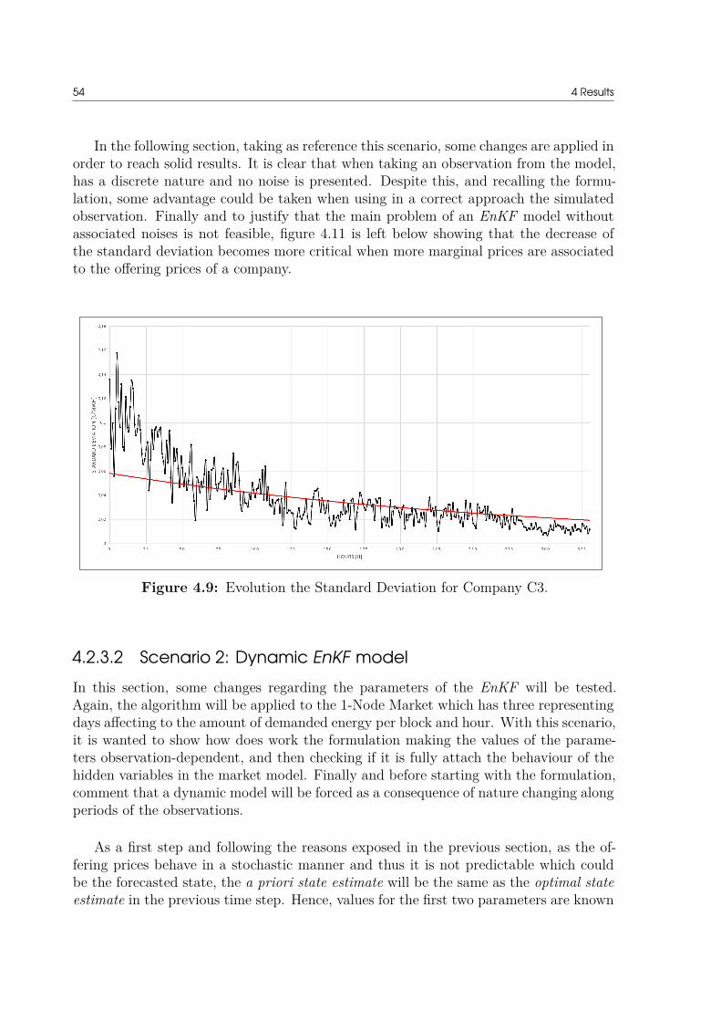
54 4 Results
In the following section, taking as reference this scenario, some changes are applied inorder to reach solid results. It is clear that when taking an observation from the model,has a discrete nature and no noise is presented. Despite this, and recalling the formu-lation, some advantage could be taken when using in a correct approach the simulatedobservation. Finally and to justify that the main problem of an EnKF model withoutassociated noises is not feasible, figure 4.11 is left below showing that the decrease ofthe standard deviation becomes more critical when more marginal prices are associatedto the offering prices of a company.
Figure 4.9: Evolution the Standard Deviation for Company C3.
4.2.3.2 Scenario 2: Dynamic EnKF modelIn this section, some changes regarding the parameters of the EnKF will be tested.Again, the algorithm will be applied to the 1-Node Market which has three representingdays affecting to the amount of demanded energy per block and hour. With this scenario,it is wanted to show how does work the formulation making the values of the parame-ters observation-dependent, and then checking if it is fully attach the behaviour of thehidden variables in the market model. Finally and before starting with the formulation,comment that a dynamic model will be forced as a consequence of nature changing alongperiods of the observations.
As a first step and following the reasons exposed in the previous section, as the of-fering prices behave in a stochastic manner and thus it is not predictable which couldbe the forecasted state, the a priori state estimate will be the same as the optimal stateestimate in the previous time step. Hence, values for the first two parameters are known

4.2 Ensemble Kalman Filter 55
an presented in table 4.5.
Mt Identity matrixQt Zero matrix
Table 4.5: EnKF Forecasting Parameters.
This will result in calculating the covariance sample matrix with the values of theoptimal state estimate matrix in t-1, which makes sense if there is not a prediction.
Next step will be to set properly the simulated observation matrix exposed in equa-tion 3.17. Its value will depend on the optimal state estimate matrix as well as parametersHt and vt. The strategy applied in this project will be the following:
• When a new market prices comes out the market, as did with the initial distribu-tions, it is associated with a company. In these steps it will be only supposed thatofferings are greater than marginal costs. At the end of the section, special caseswhich price could be lower will be studied.
• Once the market price is classified, the difference between this value and the meanvalue of the associated ensemble is calculated thus resulting in variable dt:
dt = λMt − Et(xi,j∗
t ) (4.3)
Here, the asterisk next to j indicates that the mean value will be only calculatedfrom the selected company. See that this variable can be either positive or negative,and will be used to calculate both Ht and vt.
• In order to calculate matrix Ht, it will be supposed that the last company insidethe market clearing is taking some risk in terms of price rising. This means that ashift to the mean values of all the companies in each ensemble must be done. Toinfer proportionally, a new constant is presented:
jt = 1 + dt
Et(xi,j∗t )
(4.4)
Taking as reference this constant, matrix Ht will be a diagonal one which entrieswill be identical and equal to jt:
Ht = jt ∗
1 0 0 . . . 00 1 0 . . . 0... ... ... . . . ...0 0 0 . . . 1
(4.5)

56 4 Results
• In addition, some white error vt must be added to avoid decrease in standarddeviations. As a second hypothesis, it will be supposed that the risk taken bycompanies with lower marginal costs should be lower. Therefore, to cover thisuncertainty and taking as reference the value of dt, a value for vt will be given sothat the distribution ranges from the shifted mean value until the previous one.To fulfill this premise, the following equation will be applied:
vt = Σt − d2t (4.6)
• With these determined parameters, the value of the simulated observation can becalculated and thus follow with the formulation as stated in section 3.
These steps have been exposed considering only the situations when the offering priceis greater that its corresponding marginal cost. However, as proceeded with the initialdistributions, this offered price could be lower. It is known that some energy generatingcompanies implement this action when is cheaper for them not to stop generating ratherthan being out of the market clearing. Therefore, since there is a base factor that gen-erates small demands, when this case occurs together with a market price immediatelybelow the marginal cost of any of the companies, this special case will be considered.Here, dt will be negative and as a consequence jt less than one. It is not a case thathas a high occurrence, but must be taken into account because in the current electricitymarket occurs as it may be the case of a nuclear power plant.
Finally and before commenting the results, remark that the real observation has adiscrete nature and thus must be treated. By reason of this fact, yt will collect meanvalues from the simulated observation columns of the matrix being the market price inthe associated company. This is done in this way to avoid minimizing the variancescreated with variable dt.
As was done in the previous scenario, the figure 4.10 is left with six representativeboxes of the distributions that represent the forecasts made in six simulation periods.Together with the graph, the corresponding values are left as a guide in table 4.6. In thegraph, data corresponding to March 21 has been considered, taking into account thatthe simulation begins on January 1. In this case, it has been opted for the company C4although later it will be analyzed the precision of the results for all others. However, un-like the previous scenario, looking at the graph it can be observed that the real offeringprices are within the presented distributions.

4.2 Ensemble Kalman Filter 57
Figure 4.10: Box-Whiskers plot for Company C4.
Labels 500 515 530 545 560 575Min 24,932 23,524 23,767 22,550 24,559 26,220Q1 25,460 25,020 25,691 24,012 25,097 27,068
Median 25,650 25,455 26,338 24,494 25,396 27,225Q3 25,924 26,325 26,828 24,924 25,627 27,499
Max 26,500 27,711 27,958 26,165 26,357 28,267IQR (Interquartile Range) 0,463 1,305 1,136 0,912 0,530 0,431
Real Offering Price 25,629 25,899 26,562 25,072 25,651 27,326
Table 4.6: Data Regarding Figure 4.10.
Continuing with the analysis of the results of the table, it can be seen that the valuesof the median indicates changes in prices between simulations. It no longer remainsalmost static as it could be detected in the previous scenario and it is also a potential in-dicator that the shift through the mean done by jt is being applied correctly. In addition,it can be observed that due to the special cases of low demand and prices immediatelybelow the marginal cost, the one mediated in the period 545 is below said cost. As ithas been said is a possible indicator, because it would really be the average value of thedistribution which should indicate such a situation, although checking in the databasethe average is also below and therefore would be representative of this special case.
Considering more closely the inter-quartile ranges, it can be observed that the re-spective values do not decrease along simulations. In fact, observing the values, can beseen that ranges between 0.5 and 1.3 approximately in the presented sampling. Smallvalues can indicate two different cases: the first is that the price change with respect

58 4 Results
to the previous value is small, and the other is that the company’s offer in that periodof time has a marginal character. In the cases of the graph, both in the first reference(500) and in the last two (560 and 575) the cause is due to be establishing the marketprice. It is already possible to anticipate justifiably that the offers of C4 are marginalalmost 1 out of 3 occasions. By means of these data, it can be concluded that the errorwith the reduction of the standard deviation has been corrected without increasing itsvalue excessively and without any justification.
Figure 4.11: Statistics for Scenario 2.
As has been done in the previous scenario, the statistics are left with respect tothe results of the simulations of this scenario. The percentages of market participation(blue bar) are almost identical to the previous occasion because the market is the sameand so are the demand factors. For the same reasons, the percentages that indicate themarginal character of the prices (green bar) are also practically identical to the previouscase.
Assessing now the percentage of success or what is the same, in how many timesthe true price is within the proposed distribution, the general conclusion is that it hasincreased considerably if it is compared. In the cases where the companies fix marketprices, the percentage is higher, standing at around 80 %. This correlation existed inscenario 1, but due to the changes made in the simulated observation, the effectivenessof the prediction has been increased.
On the occasions when the price is not marginal, results in a potential problem withthe application of this alternative due to the lack of references and as a consequence
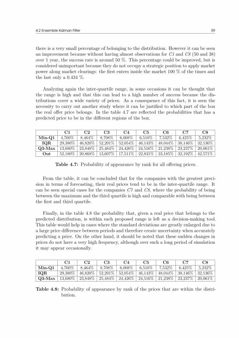
4.2 Ensemble Kalman Filter 59
there is a very small percentage of belonging to the distribution. However it can be seenan improvement because without having almost observations for C1 and C8 (50 and 38)over 1 year, the success rate is around 50 %. This percentage could be improved, but isconsidered unimportant because they do not occupy a strategic position to apply marketpower along market clearings: the first enters inside the market 100 % of the times andthe last only a 0.434 %.
Analyzing again the inter-quartile range, in some occasions it can be thought thatthe range is high and that this can lead to a high number of success because the dis-tributions cover a wide variety of prices. As a consequence of this fact, it is seen thenecessity to carry out another study where it can be justified to which part of the boxthe real offer price belongs. In the table 4.7 are reflected the probabilities that has apredicted price to be in the different regions of the box.
C1 C2 C3 C4 C5 C6 C7 C8Min-Q1 4,760% 8,464% 8,708% 6,008% 6,510% 7,532% 6,425% 5,232%
IQR 29,380% 46,820% 52,201% 52,054% 46,143% 48,044% 38,146% 32,136%Q3-Max 13,680% 23,848% 25,484% 24,426% 24,516% 21,238% 23,237% 20,061%
Out 52,180% 20,868% 13,607% 17,511% 22,831% 23,185% 32,192% 42,571%
Table 4.7: Probability of appearance by rank for all offering prices.
From the table, it can be concluded that for the companies with the greatest preci-sion in terms of forecasting, their real prices tend to be in the inter-quartile range. Itcan be seen special cases for the companies C7 and C8, where the probability of beingbetween the maximum and the third quartile is high and comparable with being betweenthe first and third quartile.
Finally, in the table 4.8 the probability that, given a real price that belongs to thepredicted distribution, is within each proposed range is left as a decision-making tool.This table would help in cases where the standard deviations are greatly enlarged due toa large price difference between periods and therefore create uncertainty when accuratelypredicting a price. On the other hand, it should be noted that these sudden changes inprices do not have a very high frequency, although over such a long period of simulationit may appear occasionally.
C1 C2 C3 C4 C5 C6 C7 C8Min-Q1 4,760% 8,464% 8,708% 6,008% 6,510% 7,532% 6,425% 5,232%IQR 29,380% 46,820% 52,201% 52,054% 46,143% 48,044% 38,146% 32,136%Q3-Max 13,680% 23,848% 25,484% 24,426% 24,516% 21,238% 23,237% 20,061%
Table 4.8: Probability of appearance by rank of the prices that are within the distri-bution.

60 4 Results
To end the section and as a guide, it is left the equivalence between a box diagramand a normal distribution in the figure 4.12 due to observing a statistical distributionis more common in comparison with a box diagram. The graphic comparison betweenthese two representations can be a useful tool to understand the box-whiskers diagram.This type of diagrams has been chosen for the presentation of results due to the fact thatthey take less space and, therefore, are particularly useful for comparing distributionsamong several groups or data sets.
Figure 4.12: Box-plot vs PDF of a Normal Distribution.[21].

4.2 Ensemble Kalman Filter 61
4.2.3.3 Scenario 3: Dynamic EnKF model with seasonal demandIn this section, the last scenario is presented where the same formulation presented inthe previous case will be applied to verify its robustness in special situations. It is knownthat sometimes there are strong fluctuations in demand that can be both predictable andnot due to different factors. Some of them can be the failure of a set of generators of apower plant, a saturated interconnection or a special day of the year where consumptionis high. In addition, it will also serve to measure performance when there is a transitionbetween seasons of the year.
For the reasons given, this section has been created where the market is going to besubjected to abrupt changes in terms of demand. For this, the demand factors used inthe 1-Node Market have been taken into account and have been altered. The figure 4.13reflects the changes made in these factors.
Figure 4.13: Demand Factors for Scenario 3.
Looking at the figure, it can be seen that the factors with respect to a day of the basetype remain unchanged. It is interesting to have a reducing factor in order to createboth smooth and sharp jumps. Regarding the factors from the Shoulder and Peak days,its value has been raised in order to increase the demands in the market. Because thestudy of this section is based on having knowledge of how the formulation of scenario2 behaves when the demands are extreme between them, the simulation has also beenopted for over a year.

62 4 Results
Finally and before commenting on the results, discuss that the randomness regard-ing the choice of the factor is no longer with respect to the day but to the time. In theprevious cases, a day factor was chosen and applied to the following 24 hours. In thiscase the factor can jump between the different days throughout the hours, being in thehour 1 a base day and in the hour 2 a peak day, for instance.
Having into consideration the new parameters added to the basic formulation ofEnKF, it can be anticipated that creating changes in demand should not change theachievement obtained previously. As it has gone up, companies with higher marginalcosts will have more opportunities to enter the market and therefore the observationswill be more distributed between them. The statistics obtained in this scenario areshown below.
Figure 4.14: Statistics for Scenario 3.
Taking into account the results of figure 4.14, it can be seen that the percentagesof success of the predicted distributions fall a bit with respect to the previous results.The reason is none other than the distribution of marginality in the offering prices. Inthe previous case, it were the companies C2, C3 and C4 the ones which set prices morefrequently and that is why it was presented a greater success in the forecasts.
Another curious fact that can be found in the graph is that the strategy suggested inscenario 2 offers similar success percentages for the extreme companies C1 and C8. Thepercentage of success of the first company is completely consistent with the strategy andpresents a value close to 50 %. While if the last one is analyzed, it offers a practicallysimilar result because from the overall achievement a 9.269 % corresponds due to itsmarginality. Therefore, it can be concluded that the more observations is had, the more

4.2 Ensemble Kalman Filter 63
chances will be presented in order to succeed in forecasting.
As this scenario shows events with very similar percentages in comparison to theprevious one, instead of a box plot it is chosen to represent some part of the resultsas shown in the figure 4.15. This chart shows the market prices, the real prices of theofferings from C3 and a pair of bands that correspond to the extremes values of theinterval [µ + 3σ, µ − 3σ] of the forecasted distribution had for this company each timestep (this interval covers approximately 99.74 % of the distribution).
Figure 4.15: Forecasted Distribution for Company C3.
Taking advantage of this type of graph and taking it as a reference will permit un-derstanding more clearly how the system works globally. Seeing the first market pricesof the graph it can be seen that there is a correlation between its increase from theirassociated marginal cost and along the bands. When these prices separate from the basevalues same behaviour is presented with the representative bands of other companies.In addition, the graph corroborates the fact that when a price is marginal the bandsbecome narrow due to there is full knowledge of the value as it is an observation. Quitethe opposite happens when the price is hidden as they spread out.
As it has been opted in the previous scenario, the table 4.9 is left where the probabil-ities of a predicted price of being in the different regions of the distribution are reflected.Since the distributions used in the graph are Gaussian, the intervals are changed. How-ever, very similar values in comparison to the previous ones are obtained as the rangesused in this table are almost aligned with the ranges of the box-whiskers used in the

64 4 Results
previous table. See the figure 4.12 as reference. Again, a forecast tendency to be aroundthe interval closer to the average is observed. Belonging to the distribution area wherethere is less uncertainty is an indicator that the shift that is made to the rest of theprices hidden in the model is appropriate.
C1 C2 C3 C4 C5 C6 C7 C8(µ-3σ,µ-σ) 5,114% 7,567% 6,887% 5,330% 6,069% 7,028% 6,019% 5,673%(µ-σ, µ+σ) 32,886% 42,768% 41,854% 44,851% 42,047% 46,617% 36,219% 34,035%
(µ+σ, µ+3σ) 15,527% 21,949% 20,528% 20,892% 22,204% 20,888% 22,145% 21,114%Out 46,473% 27,717% 30,731% 28,927% 29,680% 25,468% 35,616% 39,178%
Table 4.9: Probability of appearance by rank for all prices.
Again, along with the previous table, the 4.10 is attached where it can be seen theprobability that, belonging to a real price to the predicted distribution, is in each of thethree regions.
C1 C2 C3 C4 C5 C6 C7 C8(µ-3σ,µ-σ) 5,114% 7,567% 6,887% 5,330% 6,069% 7,028% 6,019% 5,673%(µ-σ, µ+σ) 32,886% 42,768% 41,854% 44,851% 42,047% 46,617% 36,219% 34,035%
(µ+σ, µ+3σ) 15,527% 21,949% 20,528% 20,892% 22,204% 20,888% 22,145% 21,114%
Table 4.10: Probability of appearance by rank of the prices that are within the distri-bution.
To finish with this section and to show visually how the forecasts of the offeringprices would be presented in a closing of a market clearing, the figure 4.16 is exposed.Distributions are presented by box-whisker diagrams because they are more visual forthe presentation of these type of results.
In the specific case of the figure, there is a market close where the company C3sets the price. Due to this fact, its small standard deviation can be observed again.It could be said that in this scenario, the price revelations of the first four companiesare of relevant interest in comparison with the rest. In particular, the prices of thesecompanies are within the proposed distributions.
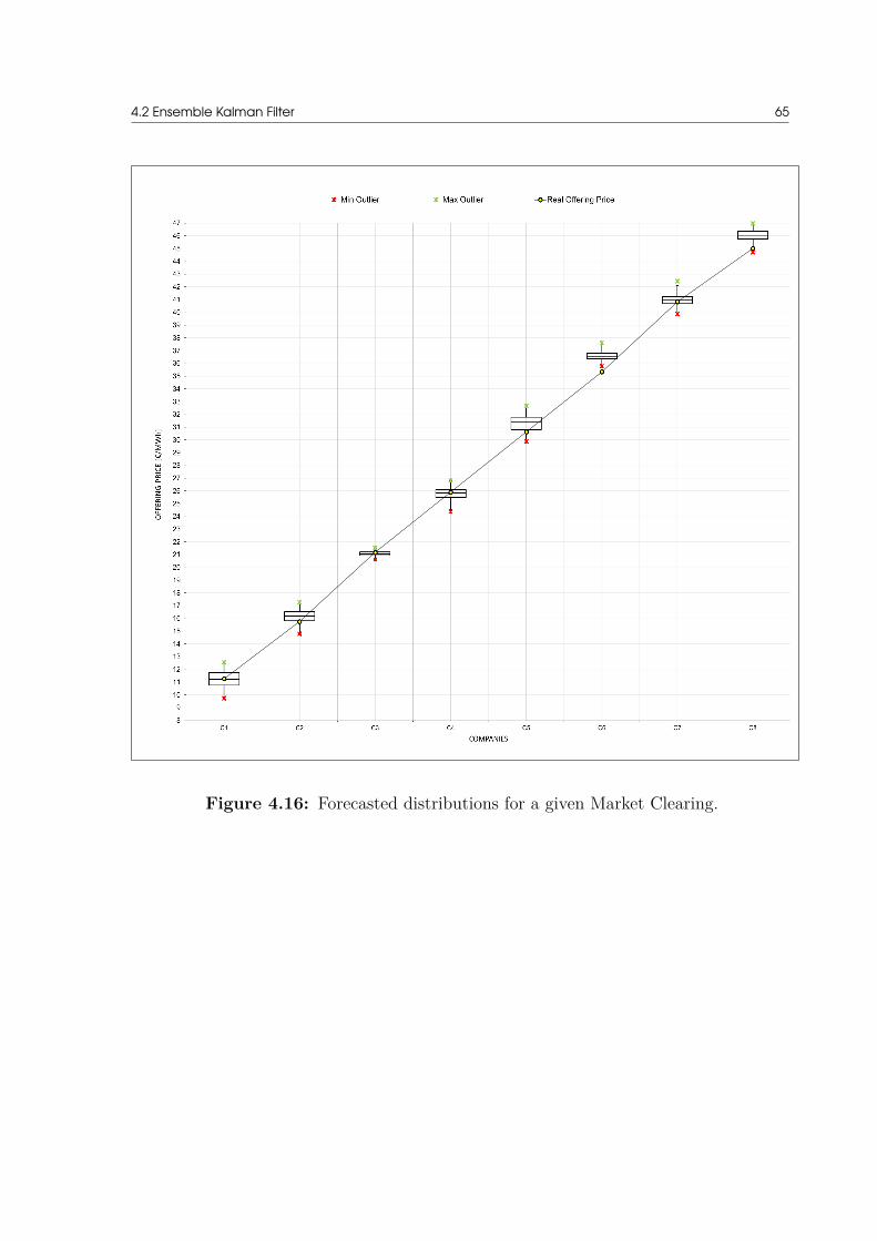
4.2 Ensemble Kalman Filter 65
Figure 4.16: Forecasted distributions for a given Market Clearing.

66

CHAPTER 5Conclusion
In this project, the novel application of an algorithm in the field of study has beenproposed for the disclosure of offering prices in a spot market. Taking as reference thework done in [8], it has been reproduced obtaining practically the same results and itsperformance has been improved by the application of an Ensemble Kalman Filter.
With respect to the implementation of the inverse Optimization problem, some de-tails have already been concluded in the results section. It has been seen that theresolution is quick and simple although it has also been seen that there are some draw-backs. The blocks that are not marginal in any period are hidden in the model andare unattainable with the proposed formulation. It also requires a lot of informationto be able to solve the optimization problem because it uses the market model in therestrictions of the main problem. Finally, and probably the most outstanding problemwith respect to the project’s objective, is that it does not disclose offering prices of therivals but their marginal prices, which is therefore irrelevant.
Seeing the potential problems found in the first methodology, they have been over-come with the implementation of EnKF. As in the Inverse Optimization Problem, a seriesof necessary hypotheses have been considered. It is assumed that a private company isable to estimate with certain error the marginal costs of its competitors. Actually, withan approximate estimate would be more than enough because when applying the EnKF,being a recursive filter, the real prices converge to their correct values. In the proposalof this project, a reduced model of an electric market is used because it would be practi-cally impossible in the development period to find and calculate all the marginal costs.
The proof that the first proposal has been improved is found in the results obtainedfor the three scenarios. It can be seen that, with a good strategy that encompassessupply values following a certain logic of market behavior, high success is achieved. Inaddition, it has been tested with different demand profiles with some distance betweenthem and the performance has been maintained. Finally, another example of perfor-mance is that the pricing of the offers in the model is done in a random way withoutfollowing any risk pattern and it is always greater than the marginal cost. Even consid-ering the ignorance of the behavior of the market prices, the percentage of success of thecompanies of interest is around 80 %.
But like all the methodologies applied in the field of engineering, there are poten-tial problems that must be prevented or detected when the results are not as expected.

68 5 Conclusion
With the application of EnKF one can have the problem of cutting the demand curvetoo much and distributing the marginality between blocks too much. As seen in theresults section, the lower the marginality, the lower the percentage of success. A pos-sible solution to this problem could be to divide the supply curve into blocks that arereally of interest to the private entity. With this, prices would only be revealed whenthe market price was associated with the most potential rivals, while if the market priceis set by a rival that is not of interest, the algorithm does not apply. With this pro-posal, in addition, a regression could be made with the revealed prices and build thefull supply curve without revealing all the prices of the blocks. There is also the pos-sibility that the market throws a series of prices with very small increases or decreases.This would lead to a decrease in the standard deviation in chain and lower the accuracyobtained. Faced with this problem, it is possible to make use of the additional param-eters proposed in the scenario 2 strategy in order to control the propagation of the same.
Making a global critique about the results obtained, it can be conclude that theEnKF is a very powerful tool to reveal prices if it is tuned properly. In fact, if a givenprivate company manages to calculate offer prices, it could be applied to a real market.It is worth noting that said applicability is of special interest to those producers thathave a significant market share and therefore are able to exercise their market power.

CHAPTER 6Conclusión
En este proyecto, se ha propuesto la aplicación novedosa de un algoritmo en el campode estudio para la divulgación de precios de oferta en un mercado spot. Tomando comoreferencia el trabajo realizado en [8], se ha reproducido obteniendo prácticamente losmismos resultados y se ha mejorado su rendimiento mediante la aplicación de un En-semble Kalman Filter.
Con respecto a la implementación del problema de optimización inversa, algunos de-talles ya se han concluido en la sección de resultados. Se ha visto que la resolución esrápida y simple aunque también se ha visto que hay algunos inconvenientes. Los bloquesque no son marginales en ningún período se ocultan en el modelo y son inalcanzablescon la formulación propuesta. También requiere mucha información para poder resolverel problema de optimización porque usa el modelo de mercado en las restricciones delproblema principal. Finalmente, y probablemente el problema más destacado con re-specto al objetivo del proyecto, es que no revela los precios de oferta de los rivales sinosus precios marginales, lo cual resulta irrelevante.
Al ver los posibles problemas encontrados en la primera metodología, se han superadocon la implementación del EnKF. Al igual que en el problema de optimización inversa,se han considerado una serie de hipótesis necesarias. Se supone que una empresa privadapuede estimar con cierto error los costos marginales de sus competidores. En realidad,con una estimación aproximada sería más que suficiente porque al aplicar el EnKF, quees un filtro recursivo, los precios reales convergen a sus valores correctos. En la prop-uesta de este proyecto, se usa un modelo reducido de un mercado eléctrico porque seríaprácticamente imposible en el período de desarrollo encontrar y calcular todos los costosmarginales.
La prueba de que la primera propuesta se ha mejorado se encuentra en los resultadosobtenidos para los tres escenarios. Se puede ver que, con una buena estrategia que abarcalos valores de suministro siguiendo una cierta lógica del comportamiento del mercado,se logra un gran éxito. Además, se ha probado con diferentes perfiles de demanda concierta distancia entre ellos y se ha mantenido el rendimiento. Finalmente, otro ejemplode desempeño es que el precio de las ofertas en el modelo se realiza de forma aleatoriasin seguir ningún patrón de riesgo y siempre es mayor que el costo marginal. Inclusoteniendo en cuenta el desconocimiento del comportamiento de los precios de mercado,el porcentaje de éxito de las empresas de interés ronda el 80 %.

70 6 Conclusión
Pero como todas las metodologías aplicadas en el campo de la ingeniería, existenproblemas potenciales que hay que prevenir o detectar cuando los resultados no son losesperados. Con la implementación del EnKF se puede tener el problema de seccionardemasiado la curva de demanda y repartir demasiado la marginalidad entre bloques.Como se ha visto en el apartado de resultados, a menor marginalidad menor porcentajede acierto. Una posible solución a este problema podría ser el dividir la curva de ofertaen bloques que realmente sean de interés para la entidad privada. Con esto, solo serevelarían ofertas cuando el precio de mercado estuviera asociado a los rivales más po-tenciales, mientras que si el precio de mercado lo fija un rival que no es de interés, elalgoritmo no se aplica. Con esta propuesta, además, se podría realizar una regresióncon los precios revelados y construir la curva de oferta al completo sin revelar todos losprecios de los bloques. También cabe la posibilidad de que el mercado arroje una seriede precios con incrementos o decrementos muy pequeños. Esto conllevaría a una dis-minución de la desviación estándar en cadena y bajaría la precisión obtenida. Ante esteproblema, se puede hacer uso de los parámetros adicionales propuestos en la estrategiadel escenario 2 con el fin de controlar la propagación de la misma.
Haciendo una critica global acerca de lo obtenido, el EnKF es una herramienta pararevelar precios muy potente si se ajusta adecuadamente. De hecho, si la una compañíaprivada dada consigue calcular precios de oferta, se podría aplicar a un mercado real.Bien cabe destacar, que dicha aplicabilidad es de especial interés para aquellos produc-tores que tienen una importante cuota de mercado y, por lo tanto, pueden ejercer supoder de mercado.

Bibliography[1] Europarl. (2018). Fact Sheets on the European Union, [Online]. Available: http:
//www.europarl.europa.eu/atyourservice/en/displayFtu.html?ftuId=intro.html (visited on November 15, 2017).
[2] S. Stoft, “Power System Economics: Designing Markets for Electricity,” January2002.
[3] D. Newbery, “Electricity liberalisation in Britain: The quest for a satisfactorywholesale market design,” The Energy Journal, volume 26, pages 43–70, 2005,issn: 01956574, 19449089. [Online]. Available: http://www.jstor.org/stable/23297006.
[4] C. Ruiz and A. J. Conejo, “Pool Strategy of a Producer With Endogenous For-mation of Locational Marginal Prices,” IEEE Transactions on Power Systems,volume 24, number 4, pages 1855–1866, November 2009, issn: 0885-8950. doi:10.1109/TPWRS.2009.2030378.
[5] H. Haghighat, “Strategic Offering Under Uncertainty in Power Markets,” Interna-tional Journal of Electrical Power Energy Systems, volume 63, number SupplementC, pages 1070–1077, 2014, issn: 0142-0615. doi: https://doi.org/10.1016/j.ijepes.2014.05.049. [Online]. Available: http://www.sciencedirect.com/science/article/pii/S0142061514003202.
[6] L. Baringo and A. J. Conejo, “Offering Strategy of Wind-Power Producer: A Multi-Stage Risk-Constrained Approach,” IEEE Transactions on Power Systems, vol-ume 31, number 2, pages 1420–1429, March 2016, issn: 0885-8950. doi: 10.1109/TPWRS.2015.2411332.
[7] L. Mitridati and P. Pinson, “A Bayesian Inference Approach to Unveil SupplyCurves in Electricity Markets,” IEEE Transactions on Power Systems, volume PP,number 99, pages 1–1, 2017, issn: 0885-8950. doi: 10.1109/TPWRS.2017.2757980.
[8] C. Ruiz, A. J. Conejo, and D. J. Bertsimas, “Revealing Rival Marginal Offer PricesVia Inverse Optimization,” IEEE Transactions on Power Systems, volume 28, num-ber 3, pages 3056–3064, August 2013, issn: 0885-8950. doi: 10.1109/TPWRS.2012.2234144.
[9] NEA/IEA/OECD, “Projected costs of generating electricity 2015,” 2015. doi:http://dx.doi.org/10.1787/cost_electricity-2015-en. [Online]. Avail-able: /content/book/cost_electricity-2015-en.

72 Bibliography
[10] J. Morales, A. J. Conejo, H. Madsen, P. Pinson, and M. Zugno, Integrating Renew-ables in Electricity Markets - Operational Problems. January 2014, isbn: 9781461494119.
[11] D. Kirschen and G. Strbac, Fundamentals of Power System Economics. Wiley,2004, isbn: 0-470-84572-4.
[12] R. K. Ahuja and J. B. Orlin, “Inverse Optimization,” Operations Research, vol-ume 49, number 5, pages 771–783, 2001. doi: 10.1287/opre.49.5.771.10607.eprint: https://doi.org/10.1287/opre.49.5.771.10607. [Online]. Available:https://doi.org/10.1287/opre.49.5.771.10607.
[13] J. R. Birge, A. Hortaçsu, and J. M. Pavlin, “Inverse Optimization for the Recoveryof Market Structure from Market Outcomes: An Application to the MISO Electric-ity Market,” Operations Research, volume 65, number 4, pages 837–855, 2017. doi:10.1287/opre.2017.1606. eprint: https://doi.org/10.1287/opre.2017.1606.[Online]. Available: https://doi.org/10.1287/opre.2017.1606.
[14] M. Katzfuss, J. R. Stroud, and C. K. Wikle, “Understanding the Ensemble KalmanFilter,” The American Statistician, volume 70, number 4, pages 350–357, 2016.doi: 10.1080/00031305.2016.1141709. eprint: https://doi.org/10.1080/00031305 . 2016 . 1141709. [Online]. Available: https : / / doi . org / 10 . 1080 /00031305.2016.1141709.
[15] G. Evensen, “The Ensemble Kalman Filter: Theoretical formulation and practicalimplementation,” Ocean Dynamics, volume 53, number 4, pages 343–367, Novem-ber 2003, issn: 1616-7228. doi: 10.1007/s10236-003-0036-9. [Online]. Available:https://doi.org/10.1007/s10236-003-0036-9.
[16] A. Tsuruta, “Application of the ensemble kalman filter in the estimation of globalmethane balance,” December 2017.
[17] A. Almendral Vazquez and A. Syversveen, “The ensemble kalman filter - theoryand applications in oil industry,” February 2018.
[18] G. Welch and G. Bishop, “An introduction to the kalman filter,” Chapel Hill, NC,USA, Tech. Rep., 1995.
[19] R. Faragher, “Understanding the basis of the kalman filter via a simple and in-tuitive derivation [lecture notes],” IEEE Signal Processing Magazine, volume 29,number 5, pages 128–132, Sep. 2012, issn: 1053-5888. doi: 10.1109/MSP.2012.2203621.
[20] J. Mandel, “A Brief Tutorial on the Ensemble Kalman Filter,” February 2009.[21] Boxplot and a probability density function (pdf) of a Normal N(0,12) Population,
https://upload.wikimedia.org/wikipedia/commons/1/1a/Boxplot_vs_PDF.svg, Accessed: 2018-02-16.