untangling the hairball: tness based asymptotic reduction of … · use. more fundamentally,...
TRANSCRIPT
Untangling the hairball: fitness based asymptotic reduction ofbiological networks
F Proulx-Giraldeau *, TJ Rademaker *, P Francois
* Equal Contribution
AbstractComplex mathematical models of interaction networks are routinely used for prediction in systemsbiology. However, it is difficult to reconcile network complexities with a formal understanding oftheir behavior. Here, we propose a simple procedure (called φ) to reduce biological models to func-tional submodules, using statistical mechanics of complex systems combined with a fitness-basedapproach inspired by in silico evolution. φ works by putting parameters or combination of param-eters to some asymptotic limit, while keeping (or slightly improving) the model performance, andrequires parameter symmetry breaking for more complex models. We illustrate φ on biochemi-cal adaptation and on different models of immune recognition by T cells. An intractable modelof immune recognition with close to a hundred individual transition rates is reduced to a simpletwo-parameter model. φ extracts three different mechanisms for early immune recognition, andautomatically discovers similar functional modules in different models of the same process, allow-ing for model classification and comparison. Our procedure can be applied to biological networksbased on rate equations using a fitness function that quantifies phenotypic performance.
IntroductionAs more and more systems-level data are becoming available, new modelling approaches havebeen developed to tackle biological complexity. A popular bottom-up route inspired by “-omics”aims at exhaustively describing and modelling parameters and interactions [1, 2]. The underly-ing assumption is that the behavior of systems taken as a whole will naturally emerge from themodelling of its underlying parts. While such approaches are rooted in biological realism, thereare well-known modelling issues. By design, complex models are challenging to study and touse. More fundamentally, connectomics does not necessarily yield clear functional informationof the ensemble, as recently exemplified in neuroscience [3]. Big models are also prone to over-fitting [4, 5], which undermines their predictive power. It is thus not clear how to tackle networkcomplexity in a predictive way, or, to quote Gunawardena [6] “ how the biological wood emergesfrom the molecular trees”.
More synthetic approaches have actually proved successful. Biological networks are known tobe modular [7], suggesting that much of the biological complexity emerges from the combinatoricsof simple functional modules. Specific examples from immunology to embryonic development
1
arX
iv:1
707.
0630
0v1
[ph
ysic
s.bi
o-ph
] 1
9 Ju
l 201
7

have shown that small and well-designed phenotypic networks can recapitulate most importantproperties of complex networks [8–10]. A fundamental argument in favor of such “phenotypicmodelling” is that biochemical networks themselves are not necessarily conserved, while theirfunction is. This is exemplified by the significant network differences in segmentation of differentvertebrates despite very similar functional roles and dynamics [11]. It suggests that the level of thephenotype is the most appropriate one and that a too detailed (gene-centric) view might not be thebest level to assess systems as a whole.
The predictive power of simple models has been theoretically studied by Sethna and co-workers,who argued that even without complete knowledge of parameters, one is able to fit experimentaldata and predict new behavior [12–15]. These ideas are inspired by recent progress in statisti-cal physics, where “parameter space compression” naturally occurs, so that dynamics of complexsystems can actually be well described with few effective parameters [16]. Methods have furtherbeen developed to generate parsimonious models based on data fitting that are able to make newpredictions [17, 18]. However such simplified models might not be easily connected to actual bio-logical networks. An alternative strategy is to enumerate [19, 20] or evolve in silico networks thatperform complex biological functions [21], using predefined biochemical grammar, and allowingfor a more direct comparison with actual biology. Such approaches typically give many results.However common network features can be identified in retrospect and as such are predictive ofbiology [21]. Nevertheless, as soon as a microscopic network-based formalism is chosen, tediouslabor is required to identify and study underlying principles and dynamics. If we had a systematicmethod to simplify/coarse-grain models of networks while preserving their functions, we couldbetter understand, compare and classify different models. This would allow us to extract dynamicprinciples underlying given phenotypes with maximum predictive power .
Inspired by a recently proposed boundary manifold approach [22], we propose a simple methodto coarse-grain phenotypic models, focusing on their functional properties via the definition of aso-called fitness. Complex networks, described by rate equations, are then reduced to much sim-pler ones that perform the same biological function. We first reduce biochemical adaptation, thenconsider the more challenging problem of absolute discrimination, an important instance being theearly immune recognition [23]. In particular, we succeed in identifying functional and mathemati-cal correspondence between different models of the same process. By categorizing and classifyingthem, we identify general principles and biological constraints for absolute discrimination. Ourapproach suggests that complex models can indeed be studied and compared using parameter re-duction, and that minimal phenotypic models can be systematically generated from more complexones. This may significantly enhance our understanding of biological dynamics from a complexnetwork description.
Materials and methods
An algorithm for fitness based asymptotic reductionTranstrum & Qiu [22, 24] studied the problem of data fitting using cellular regulatory networksmodelled as coupled ordinary differential equations. They proposed that models can be reducedby following geodesics in parameter space, using error fitting as the basis for the metric. This
2

defines the Manifold Boundary Approximation Method (abbreviated as MBAM) that extracts theminimum number of parameters compatible with data [22].
While simplifying models to fit data is crucial, it would also be useful to have a more syntheticapproach to isolate and identify functional parts of networks. This would be especially useful formodel comparison of processes where abstract functional features of the models (e.g. the qualita-tive shape of a response) might not correspond to one another, or where the underlying networksare different while they perform the same overall function [11]. We thus elaborate on the approachof [22] and describe in the following an algorithm for FItness Based Asymptotic parameter Re-duction (abbreviated as FIBAR or φ). φ does not aim at fitting data, but focuses on extractingfunctional networks, associated to a given biological function. To define biological function, werequire a general fitness (symbolized by φ) to quantify performance. Fitness is broadly definedas a mathematical quantity encoding biological function in an almost parameter independent way,which allows for a much broader search in parameter space than traditional data fitting (examplesare given in the next sections). The term fitness is inspired by its use in evolutionary algorithms toselect for coarse-grained functional networks [21]. We then define model reduction as the searchfor networks with as few parameters as possible optimizing a predefined fitness. There is no reasona priori that such a procedure would converge for arbitrary networks or fitness functions: it mightsimply not be possible to optimize a fitness without some preexisting network features. A moretraditional route to optimization would rather be to increase the number of parameters to exploremissing dimensions, rather than decrease them (see discussions in [17, 18]) . We will show how φreveals network features in known models that were explicitly designed to perform the fitness ofinterest.
Due to the absence of an explicit cost function to fit data, there is no equivalence in φ to themetric in parameter space in the MBAM allowing to incrementally update parameters. However,upon further inspection, it appears that most limits in [22] correspond to simple transformations inparameter space: single parameters disappear by putting them to 0 or∞, or by taking limits wheretheir product or ratio are constant while individual parameters go to 0 or∞. In retrospect, some ofthese transformations can be interpreted as well-known limits such as quasi-static assumptions ordimensionless reduction, but there are more subtle transformations, as will appear below.
Instead of computing geodesics in parameter space, we directly probe asymptotic limits for allparameters, either singly or in pair. Practically, we generate a new parameter set by multiplying anddividing a parameter by a large enough rescaling factor f (which is a parameter of our algorithm,we have taken f = 10 for the simulations presented here), keeping all other parameters constant,or doing the same operation on a couple of parameters.
At each step of the algorithm, we compute the behavior of the network when changing singleparameters, or any couple of parameters by factor f in both directions. We then compute the changeof fitness for each of the new models with changed parameters. In most cases, there are parametermodifications that leave the fitness unchanged or even slightly improve network behavior. Amongthis ensemble, we follow a conservative approach and select (randomly or deterministically) oneset of parameter modifications that minimizes the fitness change. We then implement parameterreduction by effectively pushing the corresponding parameters to 0 or∞, and iterate the methoduntil no further reduction enhances the fitness or leaves it unchanged, or until all parameters arereduced. The evaluation of these limits effectively removes parameters from the system whilekeeping the fitness unchanged or incrementally improving it. There are technical issues we have to
3

consider: for instance, if two parameters go to∞ some numerical choices have to be made aboutthe best way to implement this. Our choice was to keep the reduction simple : in this example,instead of defining explicitly a new parameter, we increase both parameters to a very high value,freeze one of them, and allow variation of the other one for subsequent steps of the algorithm.Another issue with asymptotic limits for rates is that corresponding divergence of variables mightoccur. To ensure proper network behavior, we thus impose overall mass conservation for somepredefined variables, e.g. total concentration of an enzyme (which effectively adds fluxes to the freeform of the considered biochemical species). We also explicitly test for convergence of differentialequations and discard parameter modifications leading to numerical divergences. Details on theimplementation of the reduction rules for specific models are presented in the Supplement and canbe automatically implemented for any model based on rate equations.
These iterations of parameter changes alone do not always lead to simpler networks. Thisis also observed in the MBAM when it is sometimes no longer possible to fit all data as wellupon parameter reduction. However, with the goal to extract minimal functional networks, we cancircumvent this problem by implementing what we call “symmetry breaking” of the parameters(Fig. 1 B-C): in most networks, different biochemical reactions are assumed to be controlledby the same parameter. An example is a kinase acting on different complexes in a proofreadingcascade with the same reaction rate. However, an alternative hypothesis is that certain steps inthe cascade are recognized to activate specific pathways, or targeted for removal (e.g. in “limitedsignalling models”, the signalling step is specifically tagged, thus having dual specificity [10]). Soto further reduce parameters, we assume that those rates, which are initially equal, can now bevaried independently by φ (Fig. 1 C). Symmetry breaking in parameter space allow us to reducemodels to a few relevant parameters/equations, and as explained below are necessary to extractsimple descriptions of network functions. Note that symmetry breaking transiently expand thenumber of parameters, allowing for a more global search for a reduced model in the complexspace of networks. Fig. 1 A summarizes this asymptotic reduction.
We have implemented φ in MATLAB for the specific cases described here, and samples ofcode used are available as Supplementary Materials.
Defining the fitnessTo illustrate the φ algorithm, we apply it to two different biological problems: biochemical adap-tation and absolute discrimination. In this section we briefly describe those problems and definethe associated fitness functions.
The first problem we study is biochemical adaptation, a classical, ubiquitous phenomenon inbiology in which an output variable returns to a fixed homeostatic value after a change of Input (seeFig. 2 A). We apply φ on models inspired by [19,24], expanding Michaelis-Menten approximationsinto additional rate equations, which further allows to account for some implicit constraints of theoriginal models, see details in the Supplement. We use a fitness that is first detailed in [25]:we measure the deviations from equilibrium at steady state ∆Oss and the maximum deviation∆Omax after a change of Input, and aim at minimizing the former while maximizing the latter.Combining both numbers into a single sum ∆Omax + ε/∆Oss gives the fitness we are maximizing(see more details in the Supplement). This simple case study illustrates how φ works and allowsus to compare our findings to previous work such as [24].
4

Fitness landscape
B
Symmetry breaking
… …
… …
C
Yes
Probe Rank
…
Select Evaluatelimit
AcceptNo
Reduce
A
Figure 1: Summary of φ algorithm. (A) Asymptotic fitness evaluation and reduction: for a givennetwork, the values of fitness φ are computed for asymptotic values of parameters or couplesof parameters. If the fitness is improved (warmer colors), one subset of improving parameters ischosen and pushed to its corresponding limits, effectively reducing the number of parameters. Thisprocess is iterated. See main text for details. (B) Parameter symmetry breaking: a given parameterpresent in multiple rate equations (here θ) is turned into multiple parameters (θ1, θ2) that can bevaried independently during asymptotic fitness evaluation. (C) Examples of parameter symmetrybreaking, considering a biochemical cascade similar to the model from [9]. See main text forcomments.
5

The second problem is absolute discrimination, defined as the sensitive and specific recognitionof signalling ligands based on one biochemical parameter. Possible instances of this problem canbe found in immune recognition between self and not self for T cells [23,26] or mast cells [27], andrecent works using chimeric DNA receptor confirm sharp thresholding based on binding times [28].More precisely, we consider models where a cell is exposed to an amount L of identical ligands,where their binding time τ defines their quality. Then the cell should discriminate only on τ , i.e.it should decide if τ is higher or lower than a critical value τc independently of ligand concentra-tion L. This is a nontrivial problem, since many ligands with binding time slightly lower than τcshould not trigger a response, while few ligands with binding time slightly higher than τc should.Absolute discrimination has direct biomedical relevance, which explains why there are models ofvarious complexities, encompassing several interesting and generic features of biochemical net-work (biochemical adaptation, proofreading, positive and negative feedback loops, combinatorics,etc.). Such models serve as ideal tests for the generality of φ.
The performance of a network performing absolute discrimination is illustrated in Fig. 2. Wecan plot the values of the network output O as a function of ligand concentration L, for differentvalues of τ (Fig. 2 B). Absolute discrimination between ligands is possible only if one (or morerealistically few) values of τ correspond to a given Output value O(L, τ) (as detailed in [23]).Intuitively, this is not possible if the dose response curves O(L, τ) are monotonic: the reason isthat for any value of output O, one can find many associated couples of (L, τ) (see Fig. 2 B).Thus, ideal performance corresponds to separated horizontal lines, encoding different values of Ofor different τ independently of L (Fig. 2 B). For suboptimal cases and optimization purposes, aprobabilistic framework is useful. Our fitness is the mutual information between the distributionof outputs O with τ for a predefined sampling of L, as proposed in [29]. If those distributions arenot well separated (meaning that we can frequently observe the same Output value for differentvalues of τ and L, Fig. 2 C top), the mutual information is low and the network performance isbad. Conversely, if those distributions are well separated ( Fig. 2 C bottom), this means that agiven Output value is statistically very often associated to a given value of τ . Then the mutualinformation is high and network performance is good. More details on this computation can befound in the Supplement (Fig. S2).
We have run φ on three different models of this process: “adaptive sorting” with one proofread-ing step [29], a simple model based on feedback by phosphatase SHP-1 from [9] (“SHP-1 model”),and a complex realistic model accounting for multiple feedbacks from [30] (“Lipniacki model”).Initial models are described in more details in following sections. We have taken published pa-rameters as initial conditions. Those three models were all explicitly designed to describe absolutediscrimination, modelled as sensitive and specific sensing of ligands of a given binding time τ [23],so ideally those networks would have perfect fitness. However due to various biochemical con-straints, these three models have very good initial (but not necessarily perfect) performance forabsolute discrimination. We see that after some initial fitness improvement, φ reaches an optimumfitness within a few steps and thus merely simplifies models while keeping constant fitness (see fit-ness values in the Supplement). We have tested φ with several parameters of the fitness functions,and we give in the following for each model the most simplified networks obtained with the help ofthose fitness functions. Complementary details and other reductions are given in the Supplement.
For both problems, φ succeeds in fully reducing the system to a single equation with essen-tially two effective parameters (see Tables in the Supplement, final model is given in the FINAL
6

A BC
once
ntra
tion
Time
Input
Output
�O
max
�Oss⌧c⌧1 < < ⌧2
Log
Out
put
Log Ligand
Log
Out
put
Log Ligand
Log Output
P(Lo
g O
utpu
t)
Outputsampling
Big overlaplow mutualinformation
No overlaphigh mutualinformation
P(Lo
g O
utpu
t)
⌧1
⌧1 ⌧2
⌧2
Log Output
Outputsampling
C
Figure 2: Fitness explanations. (A) Fitness used for biochemical adaptation. Step of an In-put variable is imposed (red dashed line) and behavior of an Output variable is computed (greenline). Maximum deviation ∆Omax and steady state deviation ∆Oss are measured and optimizedfor fitness computation. (B) Schematics of response line for absolute discrimination. We repre-sent expected dose response curves for a “bad” (top) and a “good” (bottom) model . Response todifferent binding times τ are symbolized by different colors. For the “bad” monotonic model (e.g.kinetic proofreading [31]), by setting a threshold (horizontal dashed line), multiple intersectionswith different lines corresponding to different τs are found, which means it is not possible to mea-sure τ based on the Output. Bottom corresponds to absolute discrimination: flat responses plateauat different Output values easily measure τ . Thus, the network can easily decide the position of τwith respect to a given threshold (horizontal dashed line). (C) For actual fitness computation, wesample the possible values of the Output with respect to a predefined Ligand distribution for dif-ferent τs (we have indicated threshold similar to panel (B) by a dahsed line). If the distribution arenot well separated, one can not discriminate between τs based on Outputs and mutual informationbetween Output and τ is low. If they are well separated, one can discriminate τs based on Outputand mutual information is high. See technical details in the Supplement.
OUTPUT formula, and discussion of the effective parameters in the section “Comparison and cate-gorization of models”). However, to help understanding the mathematical structure of the models,it is helpful to deconvolve some of the reduction steps from the final model. In particular, thishelps to identify functional submodules of the network that perform independent computations.Thus for each example below, we give a small set of differential equations capturing the functionalmechanisms of the reduced model . In Figures we show in the “FINAL” panel the behaviour of thefull system of ODEs including all parameters (but potentially very big or very small values afterreduction), and thus including local flux conservation.
7
Results
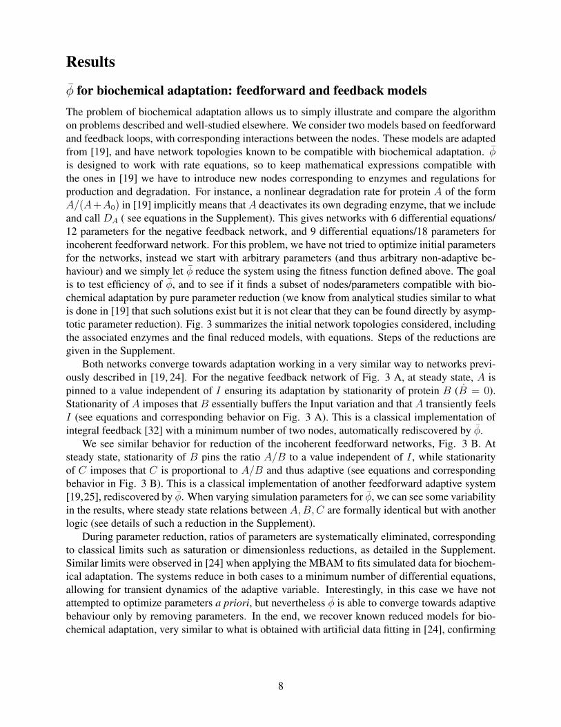
φ for biochemical adaptation: feedforward and feedback modelsThe problem of biochemical adaptation allows us to simply illustrate and compare the algorithmon problems described and well-studied elsewhere. We consider two models based on feedforwardand feedback loops, with corresponding interactions between the nodes. These models are adaptedfrom [19], and have network topologies known to be compatible with biochemical adaptation. φis designed to work with rate equations, so to keep mathematical expressions compatible withthe ones in [19] we have to introduce new nodes corresponding to enzymes and regulations forproduction and degradation. For instance, a nonlinear degradation rate for protein A of the formA/(A+A0) in [19] implicitly means that A deactivates its own degrading enzyme, that we includeand call DA ( see equations in the Supplement). This gives networks with 6 differential equations/12 parameters for the negative feedback network, and 9 differential equations/18 parameters forincoherent feedforward network. For this problem, we have not tried to optimize initial parametersfor the networks, instead we start with arbitrary parameters (and thus arbitrary non-adaptive be-haviour) and we simply let φ reduce the system using the fitness function defined above. The goalis to test efficiency of φ, and to see if it finds a subset of nodes/parameters compatible with bio-chemical adaptation by pure parameter reduction (we know from analytical studies similar to whatis done in [19] that such solutions exist but it is not clear that they can be found directly by asymp-totic parameter reduction). Fig. 3 summarizes the initial network topologies considered, includingthe associated enzymes and the final reduced models, with equations. Steps of the reductions aregiven in the Supplement.
Both networks converge towards adaptation working in a very similar way to networks previ-ously described in [19, 24]. For the negative feedback network of Fig. 3 A, at steady state, A ispinned to a value independent of I ensuring its adaptation by stationarity of protein B (B = 0).Stationarity of A imposes that B essentially buffers the Input variation and that A transiently feelsI (see equations and corresponding behavior on Fig. 3 A). This is a classical implementation ofintegral feedback [32] with a minimum number of two nodes, automatically rediscovered by φ.
We see similar behavior for reduction of the incoherent feedforward networks, Fig. 3 B. Atsteady state, stationarity of B pins the ratio A/B to a value independent of I , while stationarityof C imposes that C is proportional to A/B and thus adaptive (see equations and correspondingbehavior in Fig. 3 B). This is a classical implementation of another feedforward adaptive system[19,25], rediscovered by φ. When varying simulation parameters for φ, we can see some variabilityin the results, where steady state relations between A,B,C are formally identical but with anotherlogic (see details of such a reduction in the Supplement).
During parameter reduction, ratios of parameters are systematically eliminated, correspondingto classical limits such as saturation or dimensionless reductions, as detailed in the Supplement.Similar limits were observed in [24] when applying the MBAM to fits simulated data for biochem-ical adaptation. The systems reduce in both cases to a minimum number of differential equations,allowing for transient dynamics of the adaptive variable. Interestingly, in this case we have notattempted to optimize parameters a priori, but nevertheless φ is able to converge towards adaptivebehaviour only by removing parameters. In the end, we recover known reduced models for bio-chemical adaptation, very similar to what is obtained with artificial data fitting in [24], confirming
8

A B
ActivationDegradationRepression
Time
Concentration
Time
Concentration
A
I
B
A
I
B
Time
Concentration
C
IB
A
I
BA
Time
Concentration
BA
I
C
A = k1I � k2ABDA
DA = k03(1 � DA) � k0
4DAA
B = k05A � F0
BB = k05A � k0
6
A = k01
I
A� k0
2FA
B = k03
A
B� k0
4FB
C = k05
A
C� k0
6B
A = k01
I
A� k0
2
B = k03
A
B� k0
4
Figure 3: Adaptation networks considered and their reduction by φ. We explicitly include Produc-tion and Degradation nodes (P s and Ds) that are directly reduced into Michaelis-Menten kineticsin other works. From top to bottom, we show the original network, the reduced network, and theequations for the reduced network. Dynamics of the networks under control of a step input (I) isalso shown. Notice that the initial networks are not adaptive while the final reduced networks are.(A) Negative feedback network, including enzymes responsible for Michaelis-Menten kinetics forproduction and degradation. A is the adaptive variable. (B) Incoherent feedforward networks. Cis the adaptive variable.
9

the efficiency and robustness of fitness based asymptotic reduction.
φ for adaptive sorting
We now proceed with applications of φ to the more challenging problem of absolute discrimination.Adaptive sorting [29] is one of the simplest models of absolute discrimination. It consists of a one-step kinetic proofreading cascade [31] (converting complex C0 into C1) combined to a negativefeedforward interaction mediated by a kinase K, see Fig. 4 A for an illustration. A biologicalrealization of adaptive sorting exists for FCR receptors [27].
This model has a complete analytic description in the limit where the backward rate from C1
to C0 cancels out [29]. The dynamics of C1 is then given by:
C1 = φKKC0(L)− τ−1C1 with K = KTC∗
C0(L) + C∗ (1)
K is the activity of a kinase regulated by complex C0(L), itself proportional to ligand concen-tration L. K activity is repressed by C0 (Fig. 4, Eq. 1), implementing an incoherent feedforwardloop in the network (full system of equations are given in the Supplement).
Absolute discrimination is possible when C1 is a pure function of τ irrespective of L (so thatC1 encodes τ directly) as discussed in [23, 29]. A priori, both C0 and C1 depend on the inputligand concentration L. If we require C1 to be independent of L, the product KC0 has to become aconstant irrespective of L. This is possible becauseK is repressed by C0, so there is a “tug-of-war”on C1 production between the substrate concentration C0, and its negative effect on K. In the limitof large enough C0, K is indeed becoming inversely proportional to C0, giving a production rateof C1 independent of L. τ dependency is then encoded in the dissociation rate of C1 so that in theend C1 is a pure function of τ .
The steps of φ for adaptive sorting are summarized in Fig. 4 A. The first steps correspondto standard operations: step 1 is a quasi-static assumption on kinase concentration, step 2 bringstogether parameters having similar influence on the behavior, and step 3 is equivalent to assum-ing receptors are never saturated. Those steps are already taken in [29], and are automaticallyrediscovered by φ. Notably, we see that during reduction several effective parameters emerge, e.g.parameter A = KTφ can be identified in retrospect as the maximum possible activity of kinase K.
Step 4 is the most interesting step and corresponds to a nontrivial parameter modification spe-cific to φ, which simultaneously reinforces the two tug-of-war terms described above, so that theybalance more efficiently. This transformation solves a trade-off between sensitivity of the networkand magnitude in response, illustrated in Fig. 4 B. If one decreases only parameter C∗, the dose re-sponse curves for different τs become flatter, allowing for better separation of τs (i.e. specificity),Fig. 4 B, middle panel. However, the magnitude of the dose response curves is proportional toC∗ so that if we were to take C∗ = 0, all dose response curves would go to 0 as well and thenetwork would lose its ability to respond. It is only when both C∗ and the parameter A = KTφK
are changed in concert that we can increase specificity without losing response, Fig. 4 B, bottompanel. This ensures that K(L) becomes always proportional to L without changing the maximumproduction rate AC∗ of C1. φ finalizes the reduction by putting other parameters to limits that donot significantly change C1’s value. There is no need to perform symmetry breaking for this modelto reach optimal behavior and one-parameter reduction.
10

A
b ! 0
2.C⇤ = ↵/�1.
� = AC⇤; C⇤ ! 04.3.
5.
B = R; ! 0
A = �KKT
B
C⇤/10; KT ⇥ 10
⌧ = 3s⌧ = 5s⌧ = 10s
⌧ = 3s⌧ = 5s⌧ = 10s
C⇤/10
⌧ = 3s⌧ = 5s⌧ = 10s
Reference
⌧ = 10s⌧ = 5s⌧ = 3sK⇤ K
↵
b
�
�K
Adaptation module Kinetic sensing module
K
L
⌧�1
C0(L)
�
Figure 4: Reduction of Adaptive sorting. (A) Sketch of the network, with 5 steps of reductions byφ. Adaptation and kinetic sensing modules are indicated for comparison with reduction of othermodels. (B) Illustration of the specificity/response trade-off solved by Step 4 of φ. Compared tothe reference behavior (top panel), decreasing C∗ (middle panel) increases specificity with lessL dependency (horizontal green arrow) but globally reduces signal (vertical red arrow). If KT issimultaneously increased (bottom panel), specificity alone is increased without detrimental effecton overall response, which is the path found by φ.
11

This simple example illustrates that not only is φ able to rediscover automatically classicalreduction of nonlinear equations, but also, as illustrated by step 4 above, it is able to find a nontrivialregime of parameters where the behavior of the network can be significantly improved. Here thisis done by reinforcing simultaneously the weight of two branches of the network implicated ina crucial incoherent feedforward loop, implementing perfect adaptation, and allowing to define asimple adaptation submodule. τ dependency is encoded downstream this adaptation module in C1,defining a kinetic sensing submodule. A general feature of φ is its ability to identify and reinforcecrucial functional parts in the networks, as will be further illustrated below.
φ for SHP-1 modelThis model aims at modelling early immune recognition by T cells [9] and combines a classicalproofreading cascade [31] with a negative feedback loop (Fig. 5 A, top). The proofreading cascadeamplifies the τ dependency of the output variable, while the variable S in the negative feedbackencodes the ligand concentration L in a nontrivial way. The full network presents dose response-curves plateauing at different values for different τs, allowing for approximate discrimination asdetailed in [9] (Fig. 5 B, step 1). Full understanding of the steady state requires solving a N ×Nlinear system in combination with a polynomial equation of order N − 1, which is analyticallypossible if N is small enough (See Supplement). Behavior of the system can only be intuitivelygrasped in limits of strong negative feedback and infinite ligand concentration [9]. The logic of thenetwork appears superficially similar to the previously described adaptive sorting network, with acompetition between proofreading and feedback effects compensating for L, thus allowing for ap-proximated kinetic discrimination based on parameter τ . Other differences include the sensitivityto ligand antagonism because of the different number of proofreading steps, discussed in [23] .
When performing φ on this model, the algorithm quickly gets stuck without further reductionin the number of parameters and corresponding network complexity. By inspection of the results,it appears that the network is too symmetrical: variable S acts in exactly the same way on allproofreading steps at the same time. This creates a strong nonlinear feedback term that explainswhy the nonmonotonic dose-response curves are approximately flat as L varies as described in [9],as well as other features, such as loss of response at high ligand concentration that is sometimesobserved experimentally. This also means the output can never be made fully independent of L(see details in the Supplement). But it could also be interesting biologically to explore limits wheredephosphorylations are more specific, corresponding to breaking symmetry in parameters .
We thus perform symmetry breaking, so that φ converges in less than 15 steps, as shown in oneexample presented in Fig. 5. The dose-response curves as functions of τ become flatter while thealgorithm proceeds, until perfect absolute discrimination is reached (flat lines on Fig 5 B, step 13).
A summary of the core network extracted by φ is presented in Fig. 5 A. In brief, symmetrybreaking in parameter space concentrates the functional contribution of S in one single networkinteraction. This actually reduces the strength of the feedback, making it exactly proportional tothe concentration of the first complex in the cascade C1, allowing for a better balance between thenegative feedback and the input signal in the network.
Eventually, the dynamics of the last two complexes in the cascade are given by :
12

C4 = φ4C3 + γ5SC5 − (φ5 + τ−1)C4 with C3 ∝ C1 (2)C5 = φ5C4 − γ5SC5 with S ∝ C1 (3)
Now at steady state, φ5C4 = γ5SC5 from Eq. 3 so that those terms cancel out in Eq. 2 and weget that at steady state C4 = φ4τC3, with C3 proportional to C1 via C2 in the cascade. Lookingback at Eq. 3, it means that at steady state both the production and the degradation rates of C5
are proportional to C1 (respectively via C3 for production and S for degradation) . This is anothertug-of-war effect, so that at steady state C5 concentration is independent of C1 and thus fromL. However, there is an extra τ dependency coming from C4 at steady state (Eq. 2), so that C5
concentration is simply proportional to a power of τ (see full equations in the Supplement).Again, φ identifies and focuses on different parts of the network to perform perfect absolute
discrimination. Symmetry breaking in the parameter spaces allows to decouple identical proof-reading steps and effectively makes the behavior of the network more modular, so that only onecomplex in the cascade is responsible for the τ dependency (“kinetic sensing module” in Fig. 5)while another one carries the negative interaction of S (“Adaptation module” in Fig. 5) .
When varying initial parameters for reduction, we see different possibilities for the reduction ofthe network (see examples in the Supplement). While different branches for degradation by S canbe reinforced by φ, eventually only one of them performs perfect adaptation. Similar variability isobserved for τ sensing. Another reduction of this network is presented in the Supplement.
φ for Lipniacki modelWhile the φ algorithm works nicely on the previous examples, the models are simple enough sothat in retrospect the reduction steps might appear as natural (modulo nontrivial effects such asmass conservation or symmetry breaking). It is thus important to validate the approach on a morecomplex model which can be understood intuitively but is too complex mathematically to assesswithout simulations, a situation typical in systems biology. It is also important to apply φ to apublished model not designed by ourselves.
We thus consider a much more elaborated model for T cell recognition proposed in [30] andinspired by [33]. This models aims at describing many known interactions of receptors in a real-istic way, and accounts for several kinases such as Lck, ZAP70, ERK, and phosphatases such asSHP-1, multiple phosphorylation states of the internal ITAMs. Furthermore, this model accountsfor multimerization of receptors with the enzymes. As a consequence, there is an explosion of thenumber of cross-interactions and variables in the system, as well as associated parameters (sinceall enzymes modulate variables differently), which renders its intractable without numerical simu-lations. It is nevertheless remarkable that this model is able to predict a realistic response line (e.g.Fig. 3 in [30]), but its precise quantitative origin is unclear. The model is specified in the Sup-plement by its twenty-one equations that include a hundred odd terms corresponding to differentbiochemical interactions. With multiple runs of φ we found two variants of reduction. Figs. 6 and7 illustrate examples of those two variants, summarizing the behavior of the network at several re-duction steps. Due to the complexity of this network, we first proceed with biochemical reduction.Then we use the reduced network and perform symmetry breaking.
13

The network topology at the end of both reductions is shown in Figs. 6 and 7 with examplesof the network for various steps. Interestingly, the steps of the algorithm correspond to succes-sive simplifications of clear biological modules that appear in retrospect unnecessary for absolutediscrimination (multiple runs yield qualitatively similar steps of reduction). In both cases, we ob-serve that biochemical optimization first prunes out the ERK positive feedback module (which inthe full system amplifies response), but keeps many proofreading steps and cross-regulations. Theoptimization eventually gets stuck because of the symmetry of the system, just like we observed inthe SHP-1 model from the previous section (Fig. 6 B and Fig. 7 A ).
Symmetry breaking is then performed, and allows is to considerably reduce the combinato-rial aspects of the system, reducing the number of biochemical species and fully eliminating oneparallel proofreading cascade (Fig. 6 C) or combining two cascades (Fig. 7 B). In both vari-ants, the final steps of optimization allow for further reduction of the number of variables keepingonly one proofreading cascade in combination with a single loop feedback via the same variable(corresponding to phosphorylated SHP-1 in the complete model).
Further study of this feedback loop reveals that it is responsible for biochemical adaptation,similarly to what we observed in the case of the SHP-1 model. However, the mechanism foradaptation is different for the two different variants and corresponds to two different parameterregimes.
For the variant of Fig. 6, the algorithm converges to a local optimum for the fitness. Howeverupon inspection, the structure appears very close to the SHP-1 model reduction, and can be op-timized by putting three additional parameters to 0. The Output of the system of Fig. 6 is thengoverned by three variables out of the initial twenty-one and is summarized by:
C7 = φ1C5(L)− φ2C7 − γSC7 (4)S = λC5(L)− µRtotS (5)
CN = φ2C7 − τ−1CN (6)
Here C5(L) is one of the complex concentrations midway of the proofreading cascade (we indicatehere L dependency that can be computed by mass conservation but is irrelevant for the understand-ing of the mechanism). S is the variable accounting for phosphatase SHP-1 in the Lipniacki model,and Rtot the total number of unsaturated receptors (the reduced system with the name of the origi-nal variables is given in the Supplement).
At steady state S is proportional to C5(L) from Eq. 5. We see from Eq. 4 that the productionrate of C7 is also proportional to C5(L). Its degradation rate φ2 + γS is proportional to S ifφ2 � γS (which is the case). So both the production and degradation rates of C7 are proportional(similar to what happens in the SHP-1 model, Eq. 3), and the overall contribution of L cancels out.This corresponds to an adaptation module.
One τ dependency remains downstream of C7 through Eq. 6 (realizing a kinetic sensing mod-ule) so that the steady state concentration of CN is a pure function of τ , thus realizing absolutediscrimination. Notably, this model corresponds to a parameter regime where most receptors arefree from phosphatase SHP-1, which actually allows for the linear relationship between S and C5.
For the second variant, when the system has reached optimal fitness the same feedback loopin the model performs perfect adaptation, and the full system of equations in both reductions havesimilar structure (compare Eqs. 28 - 34 to Eqs. 35 - 43 in the Supplement). But the mechanism
14

for adaptation is different: this second reduction corresponds to a regime where receptors areessentially all titrated by SHP-1. More precisely, we have (calling Rf the free receptors, and Rp
the receptors titrated by SHP-1):
Rp = µRf (L)S − εRp (7)S = λC5 − µRf (L)S (8)C5 = C3(L)− lSC5 (9)
Now at steady state, ε is small so that almost all receptors are titrated in the form Rp, andthus Rp ' Rtot. This fixes the product Rf (L)S ∝ Rtot to a value independent of L in Eq. 7,so that at steady state of S in Eq. 8, C5 = εRtot/λ is itself fixed at a value independent of L.This implements an “integral feedback” adaptation scheme [32]. Down C5, there is a simple linearcascade where one τ dependency survives, ensuring kinetic sensing and absolute discriminationfor the final complex of the cascade.
Comparison and categorization of modelsAn interesting feature of φ is that reduction allows to formally classify and connect models ofdifferent complexities. We focus here on absolute discrimination only. Our approach allows us todistinguish at least four levels of coarse-graining for absolute discrimination, as illustrated in Fig.8.
At the upper level, we observe that all reduced absolute discrimination models considered canbe broken down into two parts of similar functional relevance. In all reduced models, we canclearly identify an adaptation module realizing perfect adaptation (defining an effective parameterλ in Fig. 8) , and a kinetic sensing module performing the sensing of τ (function f(τ) in Fig. 8).If f(τ) = τ , we get a two-parameter model, where each parameter relates to a submodule.
The models can then be divided in the nature of the adaptatation module, which gives the sec-ond level of coarse-graining. With φ, we automatically recover a dichotomy previously observedfor biochemical adaptation between feedforward and feedback models [19,25]. The second variantof Lipniacki relies on an integral feedback mechanism, where adaptation of one variable (C5) isdue to the buffering of a negative feedback variable (S(L)) (Eqs. 7 - 9, Fig. 8). Adaptive sorting,the SHP-1 model and the first variant of Lipniacki model instead rely on a “feedforward” adap-tation module where a tug-of-war between two terms (an activation term A(L) and feedforwardterms K / S in Fig. 8) exactly compensates.
The tug-of-war necessary for adaptation is realized in two different ways, which is the thirdlevel of coarse-graining. In adaptive sorting, this tug-of-war is realized at the level of the produc-tion rate of the Output, that is made ligand independent by a competition between a direct positivecontribution and an indirect negative one (Eq. 1, Fig. 8). In the reduced SHP-1 model, the con-centration of the complex C upstream the output is made L independent via a tug-of-war betweenits production and degradation rates. The exact same effect is observed in the first variant of theLipniacki model: at steady state, from Eqs. 4 and 5 the production and degradation rates of C7
are proportional (Fig. 8) which ensures adaptation. So φ allows to rigorously confirm the intuitionthat the SHP-1 model and the Lipniacki model indeed work in a similar way and belong to the
15

same category in the unsaturated receptor regime. We also notice that φ suggests a new coarse-grained model for absolute discrimination based on modulation of degradation rates, with fewerparameters and simpler behavior than the existing ones, by assuming specific dephosphorylationin the cascades (we notice that some other models have suggested specificity for the last step ofthe cascade, e.g. in limited signalling models [10]).
Importantly, the variable S, encoding for the same negative feedback in both the SHP-1 and thefirst reduction of Lipniacki model, plays a similar role in the reduced models, suggesting that twomodels of the same process, while designed with different assumptions and biochemical details,nevertheless converge to the same class of models. This variable S also is the buffering variablein the integral feedback branch of the reduction of the Lipniacki model, yet adaptation works in adifferent way for this reduction. This shows that even though the two reductions of the Lipniackimodel work in different parameter regimes and rely on different adaptive mechanisms, the samecomponents in the network play the crucial functional roles, suggesting that the approach is gen-eral. As a negative control of both the role of SHP-1 and more generally of the φ algorithm, weshow in Supplement on the SHP-1 model that reduction does not converge in the absence of the Svariable (Fig. S3).
Coarse-graining further allows us to draw connections between network components and pa-rameters for those different models. For instance, the outputs are functions of K(L)C0(L) foradaptive sorting and of C(L)
S(L)for SHP-1/Lipniacki models, where C0(L) and C(L) are in both
models concentrations of complex upstream in the cascade. So we can formally identify K(L)with S(L)−1. The immediate interpretation is that deactivating a kinase is similar to activating aphosphatase, which is intuitive but only formalized here by model reduction.
At lower levels in the reduction, complexity is increased, so that many more models are ex-pected to be connected to the same functional absolute discrimination model. For instance, whenwe run φ several times, the kinetic discrimination module on the SHP-1 model is realized on dif-ferent complexes (see several other examples in the Supplement). Also, the precise nature andposition of kinetic discriminations in the network might influence properties that we have notaccounted for in the fitness. In the Supplement, we illustrate this on ligand antagonism [34]: de-pending on the complex regulated by S in the different reduced models, and adding back kineticdiscrimination (in the form of τ−1 terms) in the remaining cascade on the reduced models, wecan observe different antagonistic behaviour, comparable with the experimentally measured an-tagonism hierarchy (Fig. S4 in Supplement). Finally, a more realistic model might account fornonspecific interactions (relieved here by parameter symmetry breaking), which might only giveapproximate biochemical adaptation (as in [9]) while still keeping the same core principles (adap-tation + kinetic discrimination) that are uncovered by φ.
DiscussionWhen we take into account all possible reactions and proteins in a biological network, a potentiallyinfinite number of different models can be generated. But it is not clear how the level of complexityrelates to the behavior of a system, nor how models of different complexities can be grasped orcompared. For instance, it is far from obvious whether a network as complex as the one from [30](Fig. 6 A) can be simply understood in any way, or if any clear design principle can be extracted
16

from it. We propose φ, a simple procedure to reduce complex networks, which is based on a fitnessfunction that defines network phenotype, and on simple coordinated parameter changes.
φ relies on the optimization of a predefined fitness that is required to encode coarse-grainedphenotypes. It performs a direct exploration of the asymptotic limit on boundary manifolds inparameter space. In silico evolution of networks teaches us that the choice of fitness is crucial forsuccessful exploration in parameter spaces and to allow for the identification of design principles[21]. Fitness should capture qualitative features of networks that can be improved incrementally;an example used here is mutual information [29]. While adjusting existing parameters or evenadding new ones (potentially leading to overfitting) could help optimizing this fitness, it is notobvious a priori that systematic removal of parameters is possible without decreasing the fitness,even for networks with initial good fitness. For both cases of biochemical adaptation and absolutediscrimination, φ is nevertheless efficient at pruning and reinforcing different network interactionsin a coordinated way while keeping an optimum fitness, finding simple limits in network space,with submodules that are easy to interpret. Reproducibility in the simplifications of the networkssuggests that the method is robust.
In the examples of SHP-1 and Lipniacki models, we notice that φ disentangles the behavior of acomplex network into two submodules with well identified functions, one in charge of adaptationand the other of kinetic discrimination. To do so, φ is able to identify and reinforce tug-of-warterms, with direct biological interpretation. This allows for a formal comparison of models. Thereduced SHP-1 model and the first reduction of the Lipniacki model have a similar feedforwardstructure, controlled by a variable corresponding to phosphatase SHP-1 defining the same biologi-cal interaction. This is reassuring since both models aim to describe early immune recognition; thiswas not obvious a priori from the complete system of equations or the considered network topol-ogy (compare Fig. 5 with Fig. 6A). These feedforward dynamics discovered by φ contrast with theoriginal feedback interpretation of the role of SHP-1 from the network topology only [9, 30, 33].Adaptive sorting, while performing the same biochemical function, works differently by adaptingthe production rate of the output, and thus belongs to another category of networks (Fig. 8).
φ is also able to identify different parameter regimes for a network performing the same func-tion, thereby uncovering an unexpected network plasticity. The two reductions of the Lipniackimodel work in a different way (one is feedforward based, the other one is feedback based), butimportantly, the crucial adaptation mechanism relies on the same node, again corresponding tophosphatase SHP-1, suggesting the predictive power of this approach irrespective of the details ofthe model. From a biological standpoint, since the same network can yield two different adaptivemechanisms depending on the parameter regime (receptors titrated or not by SHP-1), it could bethat both situations are observed. In mouse, T Cell Receptors (TCRs) do not bind to phosphataseSHP-1 without engagement of ligands [35], which would be in line with the reduction of the SHP-1model and the first variant of the Lipniacki model reduction. But we cannot exclude that a titratedregime for receptors exists, e.g. due to phenotypic plasticity [36], or that the very same networkworks in this regime in another organism. More generally, one may wonder if the parameters foundby φ are realistic in any way. In cases studied here, the values of parameters are not as importantas the regime in which the networks behave. For instance, we saw for the feedforward models thatsome specific variables have to be proportional, which requires nonsaturating enzymatic reactions.Conversely, the second reduction of the Lipniacki model requires titration of receptors by SHP-1.These are direct predictions on the dynamics of the networks, not specifically tied to the original
17

models.Since φ works by sequential modifications of parameters, we get a continuous mapping be-
tween all the models at different steps of the reduction process, via the most simplified one-parameter version of the model. By analogy with physics, φ thus “renormalizes” different networksby coarse-graining [16], possibly identifying universal classes for a given biochemical computa-tion, and defining subclasses [37]. This allows us to draw correspondences between networks withvery different topologies, formalizing ideas such as the equivalence between activation of a phos-phatase and repression of a kinase (as exemplified here by the comparison of influences of K(L)and S(L) in reduced models from Fig. 8). In systems biology, models are neither traditionallysimplified, nor are there systematic comparisons between models, in part because there is no ob-vious strategy to do so. The approach proposed here offers a solution for both comparison andreduction, which complements other strategies such as the evolution of phenotypic models [21] ordirect geometric modelling in phase space [8].
To fully reduce complex biochemical models, we have to perform symmetry breaking on pa-rameters. Similar to parameter modifications, the main roles of symmetry breaking is to reinforceand adjust dynamical regimes in different branches of the network, e.g. imposing proportional-ity to tug-of-war terms. Intuitively, symmetry breaking embeds complex networks into a higherdimensional parameter space allowing for better optimization. Much simpler networks can beobtained with this procedure, which shows in retrospect how the assumed nonspecificity in inter-actions strongly constrains the allowed behavior. Of course, in biology, some of this complexitymight also have evolutionary adaptive values, corresponding to other phenotypic features we haveneglected here, such as signal amplification. A tool like φ allows for a reductionist study of thesefeatures by specifically focusing on one phenotype of interest to extract its core working principles.Once the core principles are identified, it should be easier to complexify a model by accounting forother potential adaptive phenotypes (e.g. as is done to reduce antagonism in [29] or in Supplementin Fig. S4) .
Finally, there is a natural evolutionary interpretation of φ. In both evolutionary computationsand evolution, random parameter modifications in evolution can push single parameters to 0 or po-tentially very big values (corresponding to the∞ limit). However, it is clear from our simulationsthat concerted modifications of parameters are needed, e.g. for adaptive sorting, the simultaneousmodifications of the kinetics and the efficiency of a kinase regulation is required in Step 4 of thereduction. Evolution might select for networks explicitly coupling parameters that need to be mod-ified in concert. Conversely, there might be other constraints preventing efficient optimizations intwo directions in parameter space at the same time, due to epistatic effects. Gene duplications pro-vide an evolutionary solution to relieve such trade-offs, after which previously identical genes candiverge and specialize [38]. This clearly bears resemblance to the symmetry breaking proposedhere. For instance, having two duplicated kinases instead of one would allow to have differentphosphorylation rates in the same proofreading cascades. We also see in the examples of Figs. 5,6, and 7 that complex networks that cannot be simplified by pure parameter changes, can be im-proved by parameter symmetry breaking via decomposition into independent submodules. Similarevolutionary forces might be at play to explain the observed modularity of gene networks [7]. Morepractically, φ could be useful as a complementary tool for artificial or simulated evolution [21] tosimplify complex simulated dynamics [39].
18

Author contributionsConceptualization: PF; Methodology: TR and PF; Software,Validation, Formal Analysis, Inves-tigation: all 3 authors; Writing: PF; Funding Acquisition: FPG and PF; Project Administration,Supervision: PF.
AcknowledgmentsWe thank the members of the Francois group for their comments on the manuscript. We also thankanonymous referees for useful comments.
References[1] Karr JR, Sanghvi JC, Macklin DN, Gutschow MV, Jacobs JM, Bolival B, et al. A whole-cell
computational model predicts phenotype from genotype. Cell. 2012;150(2):389–401.
[2] Markram H, Muller E, Ramaswamy S, Reimann MW, Abdellah M, Sanchez CA, et al. Re-construction and Simulation of Neocortical Microcircuitry. Cell. 2015;163(2):456–492.
[3] Jonas E, Kording KP. Could a Neuroscientist Understand a Microprocessor? PLoS compu-tational biology. 2017;13(1):e1005268.
[4] Mayer J, Khairy K, Howard J. Drawing an elephant with four complex parameters. AmericanJournal of Physics. 2010;78(6):648–649.
[5] Lever J, Krzywinski M, Altman N. Points of Significance: Model selection and overfitting.Nature Methods. 2016;13(9):703–704.
[6] Gunawardena J. Models in biology: ’accurate descriptions of our pathetic thinking’. BMCbiology. 2013;12(1):29–29.
[7] Milo R, Shen-Orr S, Itzkovitz S, Kashtan N, Chklovskii D, Alon U. Network motifs: simplebuilding blocks of complex networks. Science. 2002;298(5594):824–827.
[8] Corson F, Siggia ED. Geometry, epistasis, and developmental patterning. Proc Natl Acad SciUSA. 2012;109(15):5568–5575.
[9] Francois P, Voisinne G, Siggia ED, Altan-Bonnet G, Vergassola M. Phenotypic model forearly T-cell activation displaying sensitivity, specificity, and antagonism. Proc Natl Acad SciUSA. 2013;110(10):E888–97.
[10] Lever M, Maini PK, van der Merwe PA, Dushek O. Phenotypic models of T cell activation.Nature Reviews Immunology. 2014;14(9):619–629.
[11] Krol AJ, Roellig D, Dequeant ML, Tassy O, Glynn E, Hattem G, et al. Evolutionary plasticityof segmentation clock networks. Development (Cambridge, England). 2011;138(13):2783–2792.
19

…
�
A…
R + L�1 �2 �5
C0 C1
⌧�1 ⌧�1 ⌧�1
�1S �2S �5S
OutputS
⌧�1 C5
C5
S
�5
�5SC4…C1(L)Adaptation
module
L
⌧�1
Kinetic sensing module
Output
B
Log(
Out
put)
Log([Ligand])
Step 1 Step 4
Step 7 Step 13 - FINAL⌧ = 10s⌧ = 5s⌧ = 3s
Figure 5: Reduction of SHP-1 model. (A) Initial model considered and final reduced model(bottom). Step 1 shows the initial dynamics. Equations can be found in the Supplement. φ (withparameter symmetry breaking) eliminates most of the feedback interactions by S, separating thefull network into an adaptation module and a kinetic sensing module. See main text for discussion.(B) Dose response curves for 3 different values of τ = 3, 5, 10s and different steps of φ reduction,showing how the curves become more and more horizontal for different τ , corresponding to bet-ter absolute discrimination. Corresponding parameter modifications are given in the Supplement.FINAL panel shows behavior of Eqs. 9-15 in the Supplement (full system including local massconservation). 20

D
# terms12
3/45/6>7
A
C
Biochemical reduction
Global symmetry breaking
Final steps
Kinetic sensing module
Log
Out
put
Log
Out
put
Log
Out
put
⌧ = 3s⌧ = 10s⌧ = 20s
step 1 step 8
step 12 step 16
step 20 step 24
step 28 step 32
step 33 step 36 - FINAL
Log Agonist
Adaptation module
B
D
P + T PT+L
PTL
P P PTLY LY LY
TP TPP
PT
P P PT TP TPP
LS LSY LSY LSY
T SSP
SP
PTLY
SPSP
PT
Z ZP
M MP MPP
EPPEPEOutput
Figure 6: Reduction of Lipniacki model. (A) Initial model considered. We indicate complexitywith coloured squared boxes that correspond to the number of individual reaction rates in eachof the corresponding differential equations for a given variable. (B) to (D) Dose response curvesfor different reduction steps. Step 1 shows the initial dynamics. From top to bottom, graphs onthe right column displays the (reduced) networks at the end of steps 16 (biochemical reduction),32 (symmetry breaking), 36 (final model). The corresponding parameter reduction steps are givenin the Supplement. FINAL panel shows behavior of Eq. 28-34 in the Supplement (full systemincluding local mass conservation).
21

step 1 step 9
step 15 step 19
step 27 step 32
step 33 step 43 - FINAL
Adaptation module
Kinetic sensing module
⌧ = 3s⌧ = 10s⌧ = 20s
Log
Out
put
Log Agonist
Symmetry breaking
Biochemical reductionA
B
Log
Out
put
Figure 7: Another reduction of the Lipniacki model starting from the same network as in Fig. 6A leading to a different adaptive mechanism. The corresponding parameter reduction steps aregiven in the Supplement. (A) Initial biochemical reduction suppresses the positive feedback loopin a similar way (compare with Fig. 6 B). (B) Symmetry breaking breaks proofreading cascadesand isolates different adaptive and kinetic modules (compare with Fig. 6 D). FINAL panel showsbehavior of Eq. 35-43 in the Supplement (full system including local mass conservation).
22

« Feedforward » « Feedback »
K⇤ K
�
↵
b
�
C = f(⌧)A(L) � SC
S / A(L)
C =A(L)
K� f�1(⌧)C
K / A(L)
…
�
⌧ = 3s⌧ = 5s⌧ = 10s
⌧ = 3s⌧ = 10s⌧ = 20s
K(L) / A(L)
⌧ = 3s⌧ = 5s⌧ = 10s⌧ = 3s⌧ = 5s⌧ = 10s
C = f(⌧)A(L)
K(L)with
« unsaturated » TCRs
« saturated » TCRs
Absolute Discrimination
C = A � f�1(⌧)C
C = �f(⌧)
S = A � RfS
Rf / A0/S
C = A0f(⌧)
Lipniacki modelSHP-1 modelAdaptive sorting
Figure 8: Categorization of networks based on φ reduction. Absolute discrimination modelsconsidered here (bottom of the tree) can all be coarse-grained into the same functional forms (top ofthe tree). Intermediate levels in reduction correspond to two different mechanisms, “feedforward”based and “feedback” based. See main text for discussion.
23

[12] Brown KS, Sethna JP. Statistical mechanical approaches to models with many poorly knownparameters. Physical Review E. 2003;68(2):021904.
[13] Brown KS, Hill CC, Calero GA, Myers CR, Lee KH, Sethna JP, et al. The statistical me-chanics of complex signaling networks: nerve growth factor signaling. Physical Biology.2004;1(3-4):184–195.
[14] Gutenkunst RN, Waterfall JJ, Casey FP, Brown KS, Myers CR, Sethna JP. Universally sloppyparameter sensitivities in systems biology models. PLoS Comput Biol. 2007;3(10):1871–1878.
[15] Transtrum MK, Machta BB, Brown KS, Daniels BC, Myers CR, Sethna JP. Perspective:Sloppiness and emergent theories in physics, biology, and beyond. The Journal of ChemicalPhysics. 2015;143(1):010901.
[16] Machta BB, Chachra R, Transtrum MK, Sethna JP. Parameter space compression underliesemergent theories and predictive models. Science. 2013;342(6158):604–607.
[17] Daniels BC, Nemenman I. Automated adaptive inference of phenomenological dynamicalmodels. Nature Communications. 2015;6:8133.
[18] Daniels BC, Nemenman I. Efficient inference of parsimonious phenomenological mod-els of cellular dynamics using S-systems and alternating regression. PLoS ONE.2015;10(3):e0119821.
[19] Ma W, Trusina A, El-Samad H, Lim WA, Tang C. Defining network topologies that canachieve biochemical adaptation. Cell. 2009;138(4):760–773.
[20] Cotterell J, Sharpe J. An atlas of gene regulatory networks reveals multiple three-gene mech-anisms for interpreting morphogen gradients. Molecular Systems Biology. 2010;6:425.
[21] Francois P. Evolving phenotypic networks in silico. Seminars in cell & developmental biol-ogy. 2014;35:90–97.
[22] Transtrum MK, Qiu P. Model reduction by manifold boundaries. Physical Review Letters.2014;113(9):098701–098701.
[23] Francois P, Altan-Bonnet G. The Case for Absolute Ligand Discrimination: ModelingInformation Processing and Decision by Immune T Cells. Journal of Statistical Physics.2016;162(5):1130–1152.
[24] Transtrum MK, Qiu P. Bridging Mechanistic and Phenomenological Models of ComplexBiological Systems. PLoS Comput Biol. 2016;12(5):e1004915.
[25] Francois P, Siggia ED. A case study of evolutionary computation of biochemical adaptation.Physical Biology. 2008;5(2):26009.
[26] Feinerman O, Germain RN, Altan-Bonnet G. Quantitative challenges in understanding liganddiscrimination by αβ T cells. Molecular Immunology. 2008;45(3):619–631.
24

[27] Torigoe C, Inman JK, Metzger H. An unusual mechanism for ligand antagonism. Science.1998;281(5376):568–572.
[28] Taylor MJ, Husain K, Gartner ZJ, Mayor S, Vale RD. Signal Transduction Through a DNA-Based T Cell Receptor. bioRxiv. 2016;.
[29] Lalanne JB, Francois P. Principles of adaptive sorting revealed by in silico evolution. PhysicalReview Letters. 2013;110(21):218102.
[30] Lipniacki T, Hat B, Faeder JR, Hlavacek WS. Stochastic effects and bistability in T cellreceptor signaling. Journal of Theoretical Biology. 2008;254(1):110–122.
[31] McKeithan TW. Kinetic proofreading in T-cell receptor signal transduction. Proc Natl AcadSci USA. 1995;92(11):5042–5046.
[32] Yi TM, Huang Y, Simon MI, Doyle J. Robust perfect adaptation in bacterial chemotaxisthrough integral feedback control. Proc Natl Acad Sci USA. 2000;97(9):4649–4653.
[33] Altan-Bonnet G, Germain RN. Modeling T cell antigen discrimination based on feedbackcontrol of digital ERK responses. PLoS Biology. 2005;3(11):e356.
[34] Francois P, Hemery M, Johnson KA, Saunders LN. Phenotypic spandrel: absolute discrimi-nation and ligand antagonism. Physical Biology. 2016;13(6):066011.
[35] Dittel BN, Stefanova I, Germain RN, Janeway CA. Cross-antagonism of a T cell cloneexpressing two distinct T cell receptors. Immunity. 1999;11(3):289–298.
[36] Feinerman O, Veiga J, Dorfman JR, Germain RN, Altan-Bonnet G. Variability and Ro-bustness in T Cell Activation from Regulated Heterogeneity in Protein Levels. Science.2008;321(5892):1081–1084.
[37] Transtrum MK, Hart G, Qiu P. Information topology identifies emergent model classes.arXiv:1409.6203.
[38] Innan H, Kondrashov F. The evolution of gene duplications: classifying and distinguishingbetween models. Nat Rev Genet. 2010;11(4):4.
[39] Sussillo D, Abbott LF. Generating coherent patterns of activity from chaotic neural networks.Neuron. 2009;63(4):544–557.
25

Supplement
July 21, 2017
1 Description of φ
In the following, we illustrate φ’s MATLAB implementation. The MATLABcode is available in the Supplementary Materials.
1.1 MATLAB Algorithm
sect:algorithm Seven functions are used:runLoopparamMODELtypecalcFitnessodeMODELtypeevalLimupdateParamcatch problems
runLoop is the main script. paramMODELtype and odeMODELtype defineparameters and associated ODEs which are problem specific. Parametersassociated to the model are initially stored in variable default, then latermodified parameters are stored in variable param and the list of removedparameters is stored in variable removed
A flowchart of the algorithm is presented in Fig. S1. In the following fivesteps we probe (1 - 3), rank, select, evaluate, accept (4), reduce and repeat(5).
1
arX
iv:1
707.
0630
0v1
[ph
ysic
s.bi
o-ph
] 1
9 Ju
l 201
7

1. Assign the parameter vector (PV) that paramMODELtype returns todefault. This point in parameter space is going to be probed.
2. The fitness landscape around the initial PV default is characterizedby the symmetric matrix fitnessmap, containing the fitness for modified pa-rameters or couples of parameters. The fitness function, on the contrary, isproblem specific, and is computed by calcFitness. Row by row, fitnessmapis filled by multiplying/dividing the parameters per entry by a reacaling fac-tor (f = 10 from the main text). The performance of each of these entriesis measured by computing the fitness with the new parameter combinationrelative to the initial fitness. A network with N parameters has 2N2 inde-pendent entries.
3. Removing a parameter is done in evalLim. With an estimate of thefitness landscape at hand found via the previous steps, the algorithm takesthe corresponding limit (to 0 or ∞) for the parameters that were rescaledby f . We consider only changes of parameters giving identical or improvedfitness. There exist four groups of two parameter limits θi, θj. In Tab. 1,the groups are presented in order of importance. When several couples ofparameters give favorable changes to the fitness, we evaluate the limit of allcouples that fall in group 1 one by one.
4. When we encounter a parameter limit in which the fitness is improved,we eliminate corresponding parameters and return to step 1. If for none ofthe couples in the parameter limits the fitness is improved, we move to themembers of group 2, the limits to infinity, and similarly when we find a pa-rameter limit that improves the fitness, we reduce and move on. Otherwisewe move to the parameter limits of groups 3 and, finally to group 4 with thesame criteria. This natural order shows our preference for removing param-eters one by one (set parameters values to zero), instead of simply rescalingthem (as products). Notice that we take a very conservative approach wherefitness can only be incrementally improved with this procedure.
The steps in evalLim are the following.
A Find the least nonnegative elements in fitnessmap
B Divide these in the groups defined above
2

Figure S 1: A flowchart of the algorithm.
C Pick a random element from the highest ranked nonempty group
D updateParam takes the PV default and a 2 × 2 block of removed asarguments and returns an updated PV to param.
E Compute a temporary fitness φnew with param.
F Decide as follows:If φnew ≥ φinit.
Accept removalReturn param and removed
If φnew < φinit.Reject removalSet fitnessmap(picked element) to inf .Repeat cycle at step A
The method we use to take asymptotic limits is described in the nextsection.
5. The returned PV becomes the new initial point in an (N − 1)-dimensional plane that is embedded inN -dimensional parameter space. Aroundthis new initial point, we will probe the fitness landscape in the next round.In removed, the removed parameters and their limits are stored such that φignores directions of reduced parameters in subsequent rounds.
3

Table 1: Four groups of two-parameter limitsGroup Operation Corresponding Limit taken
1 Division of two parameters by f (θi, θj)→ 02 Multiplication of two parameters by f (θi, θj)→∞3 Division/multiplication by f θi → 0, θj →∞4 Division/multiplication by f Rescaling keeping product θi · θj = constant
This procedure is repeated until there are no free parameters left, or untilall directions will decrease the fitness.
1.2 Taking asymptotic limits
There are two kinds of asymptotic limits: parameters are either taken to 0or to ∞. The 0 case is trivial to deal with: when a parameter is chosen tobe 0, we simply put and maintain it to 0 in the subsequent steps of φ.
In evaluating a limit to infinity, one cannot simply numerically set thisparameter to infinity, like in the case of a zero-limit. Instead, we consider alimit where this parameter is increased to such an extend that it dominatesother terms in a sum that affect the same variable; these other terms are thenremoved from the equations. More precisely, consider the following equation:
y2 = ay1 − (b+ c+ dy1)y2. (1)
In the limit of b → ∞ we replace this equation by the following differentialequation:
y2 = ay1 − by2, (2)
where b→ b′ = fb, where f is our multiplicative factor defined in the previoussection. This implements the idea that the c and dy1 terms are negligiblecompared to b.
It is important to define a vector of parameter coefficients to keep track ofthese infinities. The vector of coefficients is attached to the parameter vectorand updated in updateParam similarly. When the limit of a parameter istaken to infinity, its coefficient becomes zero, and the other terms in the sumwill disappear. Practically, Eq. 1 is rewritten as
y2 = cday1 − (cccdb+ cbcdc+ cacbccdy1)y2. (3)
4

The coefficients ca,b,c,d are initially set to 1. After evaluating the limit ofb → ∞, we set cb = 0, and the simplification from Eq. 1 to Eq. 2 indeedtakes place.
This can however create mass conservation problems in the rate equations.Consider the following equations for y4 and y5 where y4 is turned into y5 withrate r
y4 = ay3 − (r + q)y4
y5 = ry4 − dy5
(4)
In the limit where parameter q → ∞, parameter r will disappear fromthe equation of y4 potentially creating a divergence in the equations. A wayto circumvent this is to impose global mass conservation: situations wherey4 is turned into y5 correspond to signalling cascades where complexes aretransformed into one another, so that we can impose that the total quantityof complex is conserved. This effectively adds a compensating term to thecascade. We also explicitly control for divergences and discard parametersets for which variables diverge.
1.3 Choice of the path in parameter space
As shown in Section 1.1, the matrix fitnessmap is analyzed in the func-tion evalLim. This matrix is symmetrical since the upper triangular partof the matrix corresponding to parameters (k1, k2) and the lower triangu-lar part corresponding to parameters (k2, k1) give similar limits for groups2 and 4 in Tab. 1. When given the choice between sending (k1, k2) → ∞or (k2, k1) → ∞, FIBAR chooses randomly between the two, because theparameter combinations have the same change in fitness and in both cases anew parameter k1/k2 can be identified. However, because of FIBAR’s design,choosing one will result in a different exploration of parameter space in theremaining steps. By choosing the first parameter combination, φ will effec-tively freeze k1 but allows φ to keep exploring the logarithmic neighborhoodof k2. If the second combination is chosen, then the value of k2 is frozen andit is the neighborhood of k1 that will be probed. k2 and k1 may be present indifferent equations in the model, resulting in two not necessarily convergingreductions.
A choice thus needs to be made in the final parameter reduced model.This allows for introduction of some kind of stochasticity in the produced
5

networks in order to identify recurring patterns in the reduction. It can be achallenge in terms of reproducibility. One way to solve this problem is to seta fixed rule in the function evalLim (using variable seed) which is called thedeterministic method in the main article. The method of choice (random ordeterministic) is left at the discretion of the user. We indeed see differences inthe way networks are reduced, but the final structure of the reduced networksin all these cases can easily be mapped onto one another as described in themain text.
2 Mathematical definitions of fitness
In this section, we give mathematical definitions of the fitness functions usedfor both problems presented in the main text
2.1 Biochemical adaptation
For biochemical adaptation, we use a fitness very similar to the one proposedin [1].
We take as an initial input I = 0.5, then integrate for 1000 units of timeand shift I to 2. After waiting another 1000 time steps, we measure ∆Oss and∆Omax as indicated in Figure 2 in the main text, and we take as a fitness∆Omax + ε
∆Osswith ε = 0.01 for the NFBL model and ε = 0.001 for the
first variant of the reduction of the IFFL model and ε = 0.01 for the secondvariant.
2.2 Absolute discrimination
For absolute discrimination, we use a mutual information score, very similarto the one proposed in [2].
Imagine that some ligands with concentration L and binding time τ arepresented to a cell. For ligand concentrations chosen from a specified dis-tribution, we can now compute the typical output distribution pτ (O) for agiven τ . We consider log-uniformly distributed Input concentrations, inte-grate the system of equations, and generate a histogram of output values Ocorresponding to the input L. We take this as our approximation of pτ (O).
Absolute discrimination works when the typical output values O acrossthe range of L are unique for different τ . Intuitively, this means that the
6

output distributions for two binding times should overlap as little as possible,as illustrated in Fig. 2. We use these distributions for two values of τto define marginal probability distributions pτi(O) = p(O|τi). Lastly, weconsider equiprobable τis, and define p(τi, O) = p(O|τi)p(τi) = 1
2pτi(O) and
compute the mutual information between O and τ as
I(O, τ) = H(O) +H(τ)−H(O, τ) (5)
whereH is the classical Shannon entropyH(O, τ) = −∑i,O p(τi, O) log p(τi, O).Mutual information measures how much information we can recover from
one variable knowing the other. For instance, when I(O, τ) = 0, it means wecannot recover information on the value of τ by observing O, which wouldbe the case when both distributions are equal pτ1(O) = pτ2(O). Conversely,when the two distributions are fully separated, this means we can fully recoverτ by observing O. Thus, the the mutual information is at its maximum of1 bit. For partially overlapping distributions, the mutual information variesgradually between 0 to 1. The choice of mutual information allows us tofocus only on the respective positions of the distributions, and not on theirshape, average values, etc... This allows us to focus on the discriminatoryphenotype irrespective of other parameters. We very often obtain peakeddistribution in O corresponding to horizontal lines (as in the lower panel ofFig. 2); the absolute level of these lines is arbitrary.
During the reduction, we typically sampled 50 log-uniformly distributed Lon the interval [1, 104] and binned the resulting outputs O in 40 log-uniformlydistributed bins in the range [10−2, 102]. The results are largely independentfrom the number of bins or the range of the bins, as long as O remains in theneighborhood of biologically feasible values, the working range of the initialnetworks. Partly due to this loose constraint, the output of the reducednetworks was near the output of the initial networks.
3 Reductions of biochemical adaptation
In order to reproduce Michaelis-Menten kinetics for the Negative FeedbackLoop and the Incoherent Feedforward Loop models from [3], we consider amodel of linear ODEs where the dynamics of a node are mediated by anintermediary enzyme. In the models from [3], the production rates are of theform
7

Dose response curves
Log
Out
put
Log L
Log
Out
put
Log L
}
}
Uniform samplingon log scale
Uniform samplingon log scale
⌧c⌧1 < < ⌧2
Output distributions
Log Output
P(Lo
g O
utpu
t)
Log Output
P(Lo
g O
utpu
t)
p⌧2(O)
p⌧2(O)
p⌧1(O)
p⌧1(O)
Strong overlap
I(O, ⌧) << 1 bit
No overlap
I(O, ⌧) = 1 bit
Figure S 2: Illustration of the mutual information score used for absolutediscrimination. Upon sampling L from a log-uniform distribution, we inte-grate the equations, then compute histograms pτi(O) for τ1 and τ2. Fromthose joint distributions we compute the mutual information I(O, τ). If thedistribution overlap, it is not possible to distinguish well between the twoτi, which means I(O, τ) is low. If the distributions do not overlap, we canunambigously determine τ given O, thus I(O, τ) = 1 bit.
8

rateX =1−X
K + 1−X (6)
The problem with this is that this imposes X < 1, which is not enforcedby construction in [3]. To circumvent this difficulty, we slightly change theirmodel by introducing a production node PX and degradation node DX toeach node X. Both PX and DX are degraded by X. The quasi-static valuefor the production (P eq
X ) and degradation (DeqX ) nodes are:
P eqX =
K
K +X, Deq
X =K
K +X(7)
so that the full equation for X is given by
X = kpPX − kdDXX = kpK
K +X− kdX
K
K +X(8)
with kd and kp rates, which are potentially modulated by other proteins.Notice that we have included linear X dependency in the degradation. Inparticular, addition of PX ensures that the production rate is a decreasingfunction of X, as was hypothesized in [3].
4 Negative feedback loop
Initial equations for the negative feedback loop model are given by
A = k1I PA − k2ABDA
PA = k3(1− PA)− k4APA
DA = k5(1−DA)− k6ADA
B = k7APB − k8BDB
PB = k9(1− PB)− k10BPB
DB = k11(1−DB)− k12BDB.
Initial parameters are given in Tab. 2 and steps of the reduction of thismodel are given in Tab. 3.
9
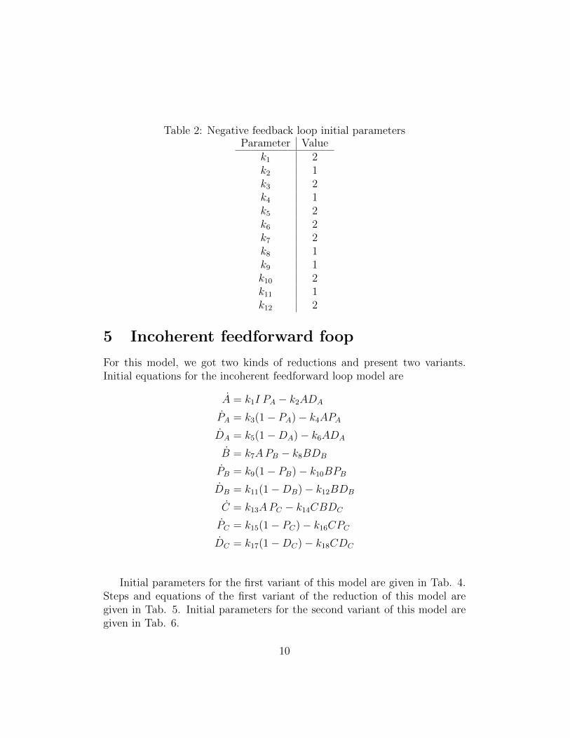
Table 2: Negative feedback loop initial parametersParameter Value
k1 2k2 1k3 2k4 1k5 2k6 2k7 2k8 1k9 1k10 2k11 1k12 2
5 Incoherent feedforward foop
For this model, we got two kinds of reductions and present two variants.Initial equations for the incoherent feedforward loop model are
A = k1I PA − k2ADA
PA = k3(1− PA)− k4APA
DA = k5(1−DA)− k6ADA
B = k7APB − k8BDB
PB = k9(1− PB)− k10BPB
DB = k11(1−DB)− k12BDB
C = k13APC − k14CBDC
PC = k15(1− PC)− k16CPC
DC = k17(1−DC)− k18CDC
Initial parameters for the first variant of this model are given in Tab. 4.Steps and equations of the first variant of the reduction of this model aregiven in Tab. 5. Initial parameters for the second variant of this model aregiven in Tab. 6.
10

Table 3: Negative feedback loop reductionStep φinit Parameters Limit Description per group
1 1.6794 (k12, k8) → ∞ DB = k11/k12B2 1.6951 (k11, k8) → (0,∞) Γ1 = k7k11/k12
3 1.6957 (k4, k9) → 0,∞ PA = 1 and PB = 14 54.4743 k10 → 05 54.4743 (k5, k6) → ∞6 54.5648 k3 → ∞7 54.6099 (k1, k2) → ∞
FINAL OUTPUT A|Beq = Γ1
k7= k8k11
k7k12
Steps of the second variant of the reduction of this model are given inTab. 7. For this variant, we took ε = 0.01 in the fitness function and slightlydifferent initial parameters. Final equations for the second variant of theIFFL reduction are given by:
A = k1I PA − k2A
PA = k3(1− PA)− k4APA
B = k7A− k8B
C = k13A− k14BC
The main difference between the two variants is on the equations for Band C. On the example of Fig. 3B in the paper, B and C regulate theirown production rate, and B titrates C, while on the system above, and Bregulates the degradation rate of C.
6 Adaptive Sorting
We perform parameter reduction on the Adaptative Sorting model withoutany symmetry breaking process. Initial equations for the adaptive sortingmodel are given by
11

Table 4: Incoherent feedforward loop first variant initial parametersParameter Value
k1 2k2 0.5k3 3k4 1k5 2k6 3k7 2k8 1k9 3k10 1k11 2k12 1k13 2k14 2k15 3k16 2k17 1k18 3
12

Table 5: Incoherent feedforward loop first variantStep φinit Parameters Limit Description per group
1 0.5958 (k14, k13) → ∞2 0.5960 (k6, k5) → ∞3 0.5961 (k15, k16) → ∞4 0.5962 (k10, k9) → ∞5 0.5971 (k13, k18) → (0,∞) DC = k17/k18C6 0.6163 (k11, k8) → (0,∞) DB = k11/k12B7 0.6169 (k18, k17) → ∞8 0.6177 (k5, k2) → (0,∞) DA = k5/k6A9 0.6699 (k17, k16) → (0,∞) PC = k15/k16C10 0.7144 (k9, k7) → (0,∞) PB = k9/k10B11 0.8544 (k4, k1) → ∞ PA = k3/k4A12 0.8670 (k3, k1) → (0,∞)13 0.8698 (k16, k7) → (0,∞)14 1.6083 (k12, k8) → ∞15 1.6094 (k8, k7) → ∞16 2.2361 (k2, k1) → ∞
FINAL OUTPUT Ceq = k8k10k11k13k15k18k7k9k12k14k16k17
K = β(KT −K)− αKC0
C0 = κ(L−∑
i
Ci)(R−∑
i
Ci) + bC1 − (φK + τ−1)C0
C1 = φKC0 − (τ−1 + b)C1.
Initial parameters are given in Tab. 8. Steps of the reduction of thismodel are given in Tab. 9.
7 SHP-1 model
7.1 SHP-1 model first reduction
We first perform parameter reduction on the SHP-1 model with global sym-metry breaking. Initial equations for the SHP-1 model are given by
13

Table 6: Incoherent feedforward loop second variant initial parametersParameter Value
k1 3k2 0.5k3 3k4 1k5 2k6 3k7 5k8 1k9 3.5k10 1k11 5k12 1k13 2k14 1k15 3k16 2k17 1k18 3
14

Table 7: Incoherent feedforward loop second variantStep φinit Parameters Limit Description per group
1 0.8788 (k14, k13) → ∞2 0.8789 (k5, k6) → ∞3 0.8793 (k9, k10) → ∞4 0.8802 (k3, k4) → ∞5 0.8811 (k4, k1) → ∞6 0.8814 (k16, k15) → ∞7 0.8822 (k18, k15) → 0,∞ PC = DC = 18 1.0372 (k11, k12) → ∞9 1.0375 k17 → ∞10 1.0378 (k2, k1) → ∞11 1.3659 (k6, k8) → 0,∞ DA = 112 1.3736 k12 → 0 DB = 113 1.4156 (k10, k1) → 0,∞ PB = 1
FINAL OUTPUT Ceq = k8k13k7k14
S = αC1(ST − S)− βSC0 = κ(L−
∑
i
Ci)(R−∑
i
Ci) + γ1SC1 − (φ1 + τ−1)C0
C1 = φ1C0 + γ2SC2 − (γ1S + φ2 + τ−1)C1
C2 = φ2C1 + γ3SC3 − (γ2S + φ3 + τ−1)C2
C3 = φ3C2 + γ4SC4 − (γ3S + φ4 + τ−1)C3
C4 = φ4C3 + γ5SC5 − (γ4S + φ5 + τ−1)C4
C5 = φ5C4 − (γ5S + τ−1)C5.
Initial parameters for this model are given in Tab. 10. Steps of the firstreduction of this model are given in Tab. 11. The final system is given bythe following equations when the reduction steps of Tab. 11 are applied.
15

Table 8: Adaptative sorting initial parametersParameter Value
φ 3× 10⁻⁴
KT 103
α 1β 1κ 10−4
R 104
b 5× 10⁻²
Table 9: Adaptive sortingStep Iinit Parameters Limit Description per group
1 0.8131 (α, β) → ∞ C∗ = β/α2 0.8131 (KT , φ) → (0,∞) A = φKT
3 0.8131 (κ,R) → (0,∞) κR→∞4 0.8131 R → ∞5 0.8645 (C∗, A) → (0,∞) λ = AC∗
6 1 α → ∞ To undo the effect C1 ∝ L for L ≤ 27 1 b → 0 Uncluttering τ
FINAL OUTPUT C1 = λτ = φKTβτ/α
S = αC1ST − βS (9)
C0 = κR(L−∑
i
Ci) + γ1SC1 − φ1C0 (10)
C1 = φ1C0 − (φ2 + γ1S)C1 (11)
C2 = φ2C1 − φ3C2 (12)
C3 = φ3C2 − φ4C3 (13)
C4 = φ4C3 + γ5SC5 − (φ5 + τ−1)C4 (14)
C5 = φ5C4 − γ5SC5. (15)
16

Table 10: SHP-1 model initial parametersParameter Value
φ 9× 10⁻²
γ 1ST 7.2× 10⁻¹
β 3× 10²
α 1β/α = C∗ 3× 10²
κ 10−4
R 3× 10⁴
Table 11: SHP-1 First reductionStep Iinit Parameters Limit Description per group
1 0.7369 (κ,R) → (0,∞)2 0.7369 γ1 → ∞3 0.8468 (φ2, φ1) → (0,∞)4 0.8583 R → ∞5 0.8583 (γ4, γ5) → 0,∞ Kinetic sensing module6 1.0000 γ2 → 0 Uncluttering τ7 1.0000 γ3 → 08 1.0000 (φ3, ST ) → ∞ Rescaling9 1.0000 (φ1, φ4) → ∞10 1.0000 β → ∞ Adaptation module11 1.0000 (φ4, ST ) → ∞12 1.0000 (ST , α) → (0,∞)
FINAL OUTPUT C5 = φ2φ5βγ5STα
τ
7.2 SHP-1 model second reduction
We then perform another reduction of the same model using a different bin-ning for the computation of the mutual information. Initial parameters andequations are identical as in the previous reduction presented in section 7.1.Steps for this reduction are given in Tab. 12.
The final system is given by the following equations when the reductionsteps given in Tab. 12 are applied.
17

Table 12: SHP-1 Second reductionStep Iinit Parameters Limit Description per group
1 0.6328 (κ,R) → (0,∞)2 0.6328 R → ∞3 0.6375 (γ4, α) → (0,∞)4 0.6464 (γ2, γ1) → 0,∞5 0.7264 γ5 → ∞ Adaptive module6 1.0000 γ3 → 07 1.0000 (φ1, β) → ∞8 1.0000 φ4 → ∞ Kinetic sensing module9 1.0000 (φ3, ST ) → ∞10 1.0000 (ST , β) → ∞11 1.0000 (φ5, β) → (0,∞)12 1.0000 (β, φ2) → (0,∞)
FINAL OUTPUT C5 = φ2φ5βγ5STα
τ
S = αC1ST − βS (16)
C0 = κR(L−∑
i
Ci) + γ1SC1 − φ1C0 (17)
C1 = φ1C0 − (φ2 + γ1S)C1 (18)
C2 = φ2C1 − φ3C2 (19)
C3 = φ3C2 + γ4SC4 − φ4C3 (20)
C4 = φ4C3 + γ5SC5 − (φ5 + γ4S + τ−1)C4 (21)
C5 = φ5C4 − γ5SC5. (22)
7.3 SHP-1 model third reduction
We perform another reduction of the same model using slightly differentinitial parameter values. All parameters are given in Tab. 10 with ST → 5ST .Initial set of equations is identical as in Sections 7.1 and 7.2. Steps for thisreduction are given in Tab. 13.
The final system is given by the following equations when the reductionsteps given in Tab. 13 are applied.
18

Table 13: SHP-1 Third reductionStep Iinit Parameters Limit Description per group
1 0.4946 (β, α) → ∞2 0.4946 (R, κ) → (0,∞)3 0.4946 (γ1, γ5) → 0 Kinetic sensing module4 1.0000 (κ, φ1) → ∞5 1.0000 φ1 → ∞6 1.0000 (φ2, φ4) → (0,∞)7 1.0000 (φ5, γ3) → ∞ Adaptation module8 1.0000 γ2 → 09 1.0000 ST → ∞10 1.0000 γ4 → 011 1.0000 (φ4, φ3) → (0,∞) Rescaling12 1.0000 (α, γ3) → (0,∞)
FINAL OUTPUT C5 = φ2φ3φ4βγ3STα
τ 2
S = αC1ST − βSC0 = κ(L−
∑
i
Ci)(R−∑
i
Ci)− φ1C0
C1 = φ1C0 − (φ2 + τ−1)C1
C2 = φ2C1 + γ3SC3 − (φ3 + τ−1)C2
C3 = φ3C2 +−γ3SC3
C4 = φ4C3 − φ5C4
C5 = φ5C4 − τ−1C5.
7.4 SHP-1 model reduction without feedback
We perform a reduction of the SHP-1 model with the SHP-1 mediated feed-back turned off. Parameter values are given in Tab. 10 with ST = 0. Thenetwork topology is as in Fig. S 3A and the corresponding initial set ofequations is identical as in Sections 7.1 and 7.2. Fig. S 3B shows that the re-duction does not converge when crucial network elements (SHP-1 feedback)are missing.
19

…A
B
⌧ = 10s ⌧ = 5s ⌧ = 3s
step 1 step 7Log
Out
put
Log Agonist
SHP-1 reduction with ST = 0
Figure S 3: “Negative control” for SHP-1 model: we attempt to reduce thismodel with φ in absence of SHP-1 (corresponding to pure kinetic proofread-ing). The algorithm fails to optimize behavior and fitness, indicating that itis not possible to do so for arbitrary networks.
20
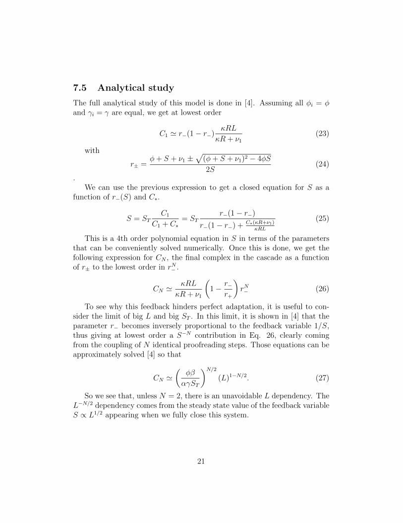
7.5 Analytical study
The full analytical study of this model is done in [4]. Assuming all φi = φand γi = γ are equal, we get at lowest order
C1 ' r−(1− r−)κRL
κR + ν1
(23)
with
r± =φ+ S + ν1 ±
√(φ+ S + ν1)2 − 4φS
2S(24)
.We can use the previous expression to get a closed equation for S as a
function of r−(S) and C∗.
S = STC1
C1 + C∗= ST
r−(1− r−)
r−(1− r−) + C∗(κR+ν1)κRL
(25)
This is a 4th order polynomial equation in S in terms of the parametersthat can be conveniently solved numerically. Once this is done, we get thefollowing expression for CN , the final complex in the cascade as a functionof r± to the lowest order in rN− .
CN 'κRL
κR + ν1
(1− r−
r+
)rN− (26)
To see why this feedback hinders perfect adaptation, it is useful to con-sider the limit of big L and big ST . In this limit, it is shown in [4] that theparameter r− becomes inversely proportional to the feedback variable 1/S,thus giving at lowest order a S−N contribution in Eq. 26, clearly comingfrom the coupling of N identical proofreading steps. Those equations can beapproximately solved [4] so that
CN '(
φβ
αγST
)N/2(L)1−N/2. (27)
So we see that, unless N = 2, there is an unavoidable L dependency. TheL−N/2 dependency comes from the steady state value of the feedback variableS ∝ L1/2 appearing when we fully close this system.
21

8 Lipniacki model
In this section, we present two parameter reductions performed by φ. Initialequations for the Lipniacki model are:
X2 = b1 pMHCfree TCRfree + (s2 + s3)X23 − (lb LCKfree + ly1X29 + τ−1)X2
X3 = lb LCKfreeX2 + ls1X4 + (s2 + s3)X24 − (ly2 +X37 + ly1X29 + τ−1)X3
X4 = X37X3 − (ly2 + ls1 + τ−1)X4
X5 = ly2X3 + ls1X6 − (tp+X37 + ly1X29 + τ−1)X5
X6 = ly2X4 +X37X5 − (tp+ ls1 + τ−1)X6
X7 = tpX5 + ls1X8 − (tp+X37 + ly1X29 + τ−1)X7
X8 = tpX6 +X37X7 − (tp+ ls1 + τ−1)X8
X9 = tpX7 + ls1X8 − (τ−1 +X37 + ly1X29 + τ−1)X9
X10 = tpX8 +X37X9 − (ls1 + τ−1)X10
X22 = ly1X29 TCRfree + τ−1(X23 +X24)− (s2 + s3)X22
X23 = ly1X29X2 − (s2 + s3 + τ−1)X23
X24 = ly1X29(X3 +X5 +X7 +X9)− (s2 + s3 + τ−1)X24
X29 = s1(X5 +X7 +X9)SHPfree + s3(X22 +X23 +X24) + s0 SHPfree
− ly1(X2 +X3 +X5 +X7 +X9 + TCRfree)X29 − s2X29
X31 = z1(X9 +X10)(m1 −X31) + z0m1 − (z0 + z2)X31
X33 = 2X31(e1 −X34) + 2m2X34 − (m2 + 3X31)X33
X34 = X31X33 − 2m2X34
X36 = 2X34(ls2 −X37) + 2e2X37 − (e2 + 2X34)X36
X37 = X34X36 − 2e2X37
22

To ensure physical behavior throughout the reduction process, we manu-ally implement the following mass conservation laws.
pMHCfree = pMHC −(
10∑
i=2
Xi +X23 +X24
)
TCRfree = TCR−(
10∑
i=2
Xi +X22 +X23 +X24
)
LCKfree = LCK −(
10∑
i=3
Xi +X24
)
SHPfree = SHP − (X22 +X23 +X24 +X29)
ZAPfree = ZAP −X31
MEKfree = MEK − (X33 +X34)
ERKfree = ERK − (X36 +X37)
We also perform initial rescaling of equations X31 to X37 to save φ steps:
X31 →m1X31
ZAP
X33 →e1X33
MEK
X34 →e1X34
MEK
X36 →ls2X36
ERK
X37 →ls2X37
ERK
Initial parameters are given in Tab. 14.
8.1 Lipniacki model reduction: first variant
For this reduction, we used mutual information as a fitness function. Wediscarded all values of the output below the measurable threshold 10−2, andused 40 log-uniformly distributed bins on the interval [10−2, 102] for the com-putation of the Output distribution. The Input concentrations were givenby 50 log-uniformly distributed values on the interval [1, 104].
23

Steps of the first biochemical reduction of this model (odeLIPbasic.m inthe MATLAB code) are given in Tab. 15. The results of the biochemicalreduction are given by
X2 = b1 pMHCfree TCR + s22X23 − lbX2
X3 = lbX2 + s23X24 − ly21X3
X4 = X37X3 − ly22X4
X5 = ly21X3 − (tp1 +X37 + ly14X29 + τ−1)X5
X6 = ly22X4 +X37X5 − (tp2 + τ−1)X6
X7 = tp1X5 − (tp3 +X37 + ly15X29 + τ−1)X7
X8 = tp2X6 +X37X7 − (tp4 + τ−1)X8
X9 = tp3X7 − (τ−1 +X37 + ly16X29)X9
X10 = tp4X8 +X37X9 − τ−1X10
X23 = ly12X29X2 − (s22 + τ−1)X23
X24 = (ly13X3 + ly14X5 + ly15X7 + ly16X9)X29 − (s23 + τ−1)X24
X29 = s11X5 + s12X7 + s13X9 − ly11TCRX29.
We then perform global symmetry breaking (odeLIPadvanced in the MAT-LAB code). Steps of reduction are given in Tab. 16.
Global symmetry breaking results in the following system.
X2 = b1 pMHCfree TCR− lbX2
X3 = lbX2 − ly2X3
X5 = ly2X3 − ly13X29X5
X7 = tp1X5 − (tp2 + ly14X29 + τ−1)X7
X9 = tp2X7 − (ly15X29 + τ−1)X9
X23 = ly12X29X2 − τ−1X23
X24 = ly13X29X5 − τ−1X24
X29 = s1X5 − ly11TCRX29
Only four more steps of reduction are needed to reach perfect adaptation,namely (ly13, ly15)→ 0, (ly11, ly14)→∞, (tp1, ly14)→∞ and finally ly14 →
24

∞. We apply those steps of reduction by hand and reach the final followingsystem.
X2 = b1 pMHCfree TCR− lbX2 (28)
X3 = lbX2 − ly2X3 (29)
X5 = ly2X3 − tp1X5 (30)
X7 = tp1X5 − ly14X29X7 − tp2X7 (31)
X9 = tp2X7 − τ−1X9 (32)
X24 = ly14X7X29 − τ−1X24 (33)
X29 = s1X5 − ly11TCRX29 (34)
8.2 Lipniacki model reduction: second variant
Initial equations, parameters, mass conservation laws and equation transfor-mations for this reduction are the same as for the previous Lipniacki reduc-tion. For this reduction, we chose mutual information as the fitness with40 bins log-uniformly distributed on the interval [10−2, 102], plus a lower binfor concentrations below 10−2 and a higher bin for concentrations above 102.We chose 50 log-uniformly distributed Input concentrations on the interval[1, 104]. Because of the binning choice, the fitness, was optimized quicker,while most reduction took place in the neutral fitness landscape of maximumfitness of 1 bit. The details of this biochemical reduction are given in Tab.17.
After the first reduction, the system is reduced to
25

X2 = b1 pMHCfree TCRfree + (s22 + s32)X23 − lb LCK X2
X3 = lb LCK X2 + ls11X4 + (s23 + s33)X24 − (ly21 +X37 + ly11X29 + τ−1)X3
X4 = X37X3 − (ly22 + ls11 + τ−1)X4
X5 = ly21X3 + ls12X6 − (tp1 +X37 + ly12X29 + τ−1)X5
X6 = ly22X4 +X37X5 − (tp2 + ls12 + τ−1)X6
X7 = tp1X5 + ls13X8 − (tp3 +X37 + ly13X29 + τ−1)X7
X8 = tp2X6 +X37X7 − (tp4 + ls13 + τ−1)X8
X9 = tp3X7 + ls14X8 − (X37 + ly14X29 + τ−1)X9
X10 = tp4X8 +X37X9 − (ls14 + τ−1)X10
X22 = ly15X29 TCRfree + τ−1(X23 +X24)− (s21 + s31)X22
X23 = ly16X29X2 − (s22 + s32 + τ−1)X23
X24 = X29(ly11X3 + ly12X5 + ly13X7 + ly14X9)− (s23 + s33 + τ−1)X24
X29 = (s11X5 + s12X7 + s13X9)SHP + (s31X22 + s32X23 + s33X24)
− (ly16X2 + ly11X3 + ly12X5 + ly13X7 + ly14X9 + ly15TCRfree)X29 − s24X29
X37 = 0.05
We then perform global symmetry breaking on this system. Steps of thebiochemical reduction of this model are given in Tab. 18
We can remove equations for X4, X6, X23 and X24 as they are dead endsin the network. X37 = 0.5 is held constant. The final expression of theoutput given in Tab. 18 is extracted from remaining equations at steady-state; expanding the equations for the relevant cascade we get
26

X2 = b1 pMHCfree TCRfree − lb LCK X2 (35)
X3 = lb LCK X2 − ly21X3 (36)
X5 = ly21X3 − ly12X29X5 (37)
X7 = tp1X5 −X37X7 (38)
X8 = X37X7 − tp4X8 (39)
X10 = tp4X8 − τ−1X10 (40)
X22 = ly15X29 TCRfree − s21X22 (41)
X29 = s11X5 SHP − ly15TCRfreeX29 (42)
X37 = 0.5 (43)
The output here is X10. Variables X22, X29 and X5 respectively correspondto variables Rp, S and C5 in the main text. The structure of Eqs. 35 to 42 isclearly very similar to the equations of the previous reduction 28 to 34, with alinear cascade for the second reduction X2 → X3 → X5 → X7 → X8 → X10
and X2 → X3 → X5 → X7 → X9 for the first reduction, modulated by aparallel loop via X29 and X5. As described in the main text, the structuraldifference comes from the mechanism of this loop, the first reduction givingan effective feedforward adaptive system, while the second reduction is anintegral feedback mechanism.
9 Antagonism
The models we reduce have all captured the phenomenon of ligand antago-nism, where the response of agonist ligands in the presence of high amountsof well chosen subthreshold ligands (i.e. with binding time lower than criti-cal binding time τc triggering response) is antagonized. With our fitness, wehave quantified and selected for absolute discrimination in the networks, andthrough the reduction, ligand antagonism has remained, but the hierarchy ofantagonism has changed. In the simplest systems, antagonism is maximumfor minimum τ , while for more complex models there maximum antagonismis reached closer to threshold τc (see discussion in [5]). It turns out we canrecover this property by adding two terms to the final reduced equations.
An overview of antagonism is presented in Fig. S4. We draw the responseline as a binary activation by choosing a threshold of the final output for ac-
27

tivation (we know from our previous works [2, 4] that adding stochasticity tohave a more probabilistic view does not fundamentally change this picture).The earliest response (in terms of ligand concentration) always comes fromthe agonist alone. Note how T cells in Fig. S4 A presented to OVA ago-nists + strong G4 antagonists are activated at higher agonist concentrationthan the weak E1 antagonists, and G4 have a binding time close to thresholdthan E1. This hierarchy is typical for experimentally observed antagonism:antagonism strength is large just below τc, the critical binding time abovewhich a response is elicited.
Similarly, in the full models for SHP-1 and Lipniacki (Fig. S4 B - C), wehave the same hierarchy. However, for the same binding times in reducedSHP-1 (Fig. S4 E) and reduced Lipniacki (Fig. S4 F), we have an invertedhierarchy, where ligands further below are more antagonizing, so closer tothe naive models discussed in [5].
It turns out that the position of the adaptive module m in the kineticproofreading cascade of N complexes, defined as the complex on which thevariable S implements the negative ”tug-of-war” term described in the maintext, determines the antagonism strength, like in Fig. 4 of ref. [5]. We canrescue the correct hierarchy of antagonism by adding kinetic terms τ−1 tothe equations. We illustrate this on the second variant of SHP-1 reduction.The antagonism hierarchy is initially absent from the reduced model (Fig.S4 G). When we add τ−1 terms to Eqs. 17 and 18, it is retrieved, Fig. 4,because m = 4 is large enough. When m is too low (m = 2, Figs. S4 E - F),antagonism behavior peaks for τ � τc and we can not recover the hierarchyobserved experimentally.
References
[1] Paul Francois and Eric D Siggia. A case study of evolutionary computa-tion of biochemical adaptation. Physical Biology, 5(2):26009, 2008.
[2] Jean-Benoıt Lalanne and Paul Francois. Principles of adaptive sortingrevealed by in silico evolution. Physical Review Letters, 110(21):218102,May 2013.
[3] Wenzhe Ma, Ala Trusina, Hana El-Samad, Wendell A Lim, and ChaoTang. Defining network topologies that can achieve biochemical adapta-tion. Cell, 138(4):760–773, August 2009.
28

OVA alone
OVA + G4
OVA + E1
Reduced model
with added
Full model
Bin
ary
activ
atio
nSH
P-1
Lipn
iack
i
1
0
⌧ = 20s
+ ⌧ = 5s
+ ⌧ = 1s
Experimental data
Bin
ary
activ
atio
n
1
0
⌧ without added ⌧
SHP-
1
Log Agonist
1
0Bin
ary
activ
atio
n
1
0Bin
ary
activ
atio
n
Agonist concentration
⌧ = 10s
+ ⌧ = 3s
+ ⌧ = 0.3s
⌧ = 10s
+ ⌧ = 3s
+ ⌧ = 0.3s
Agonist alone + strong antagonist + weak antagonist
A B
C
D
E
F
G
Figure S4: Overview of antagonism. Red corresponds to agonists alone, greento agonists in the presence of a fixed number of strong antagonist ligands andblue to agonists with weak antagonists. The output is shown as an binaryactivation depending on threshold crossing. (A) Experimental data, repro-duced from Fig. 5B of [4]. (B)-(C) Full SHP-1/Lipniacki model, showingtypical antagonistic hierarchy with binding times as in (E),(F), which showreduced variants of the SHP-1/Lipniacki model via global symmetry break-ing. (D),(G) Second variant of the reduced SHP-1 model. Upon addingback terms in τ to Eqs. 17-18, we retrieve the proper hierarchy of antag-onism. We added 104 antagonist ligands to SHP-1 models, 102 antagonistligands to Lipniacki models and 10µmol antagonist ligand concentration inthe experiments. 29

[4] Paul Francois, Guillaume Voisinne, Eric D Siggia, Gregoire Altan-Bonnet,and Massimo Vergassola. Phenotypic model for early T-cell activationdisplaying sensitivity, specificity, and antagonism. Proc Natl Acad SciUSA, 110(10):E888–97, March 2013.
[5] Paul Francois, Mathieu Hemery, Kyle A Johnson, Laura N Saunders. Phe-notypic spandrel: absolute discrimination and ligand antagonism. Phys-ical Biology. 2016;13(6):066011.
30

Table 14: Lipniacki model initial parametersParameter Value DetailsTCR 3× 10⁴
LCK 105
SHP 3× 10⁵
ZAP 105
MEK 105 Can’t be modified by φERK 3× 10⁵
b1 3× 10⁻¹/TCR Agonist peptide bindinglb 3× 10⁻¹/LCK LCK(s) bindingly1 5/SHP pSHP complex bindingly2 3× 10⁻¹ Theorine phosphorylation at complexls1 10−1 Spontaneous serine dephosphorylationls2 5× 10⁻¹ ppERK catalyzed serine phosphorylationtp 5× 10⁻² TCR phosphorylations0 10−5 Spontaneous SHP phosphorylations1 3× 10²/SHP SHP phosphorylations2 6× 10⁻⁴ SHP dephosphorylations3 5× 10⁻² SHP dissociationz0 2× 10⁻⁶ Spontaneous ZAP phosporylationz1 5/ZAP ZAP phosphorylationz2 2× 10⁻² ZAP dephosphorylationm1 5× ZAP/MEK MEK phosphorylationm2 2× 10⁻² MEK dephosphorylatione1 5×MEK/ERK ERK phosphorylatione2 2× 10⁻² ERK dephosphorylation
31

Table 15: Lipniacki basic first variantStep Iinit Parameters Limit Description per group
1 0.45 (m1,m2) → ∞2 0.47 b1 → ∞3 0.47 (lb, LCK) → (0,∞) lb′ = lb LCK4 0.47 ls1, z1 → 0,∞ Turning off the positive feedback5 0.50 e1, e2 → 06 0.50 z0, z2 → 07 0.50 m1 → 08 0.50 s3 → 09 0.50 (ls2, LCK) → (0,∞)10 0.50 ly2 → ∞11 0.50 (TCR, SHP ) → ∞12 0.5017 s0 → 013 0.5017 (s2, ly1) → (0,∞) Products14 0.5017 (SHP, s1) → (0,∞) s′1 = s1SHP15 0.5017 (LCK, ly1) → (0,∞)16 0.5216 s1 → ∞
32

Table 16: Lipniacki advanced first variantStep Iinit Parameters Limit Description per group
1 0.5837 (s22, s23) → 02 0.5837 (b1, ly22) → ∞ ly22 →∞ makes no change3 0.5837 (s21, ly22) → ∞4 0.5837 ly22 → ∞5 0.5837 (TCR, ly11) → (0,∞) ly′11 = ly11TCR6 0.5837 s12 → 07 0.6097 s13 → 08 0.6147 (tp2, tp3) → (0,∞)9 0.6231 (ly13, lb) → 0,∞10 0.6245 (tp4, ls2) → (0,∞) Products11 0.6246 (tp3, ly16) → (0,∞)12 0.6354 (ly16, ly15) → (0,∞)13 0.6563 (ly15, ly13) → (0,∞)14 0.6699 ly21 → ∞15 0.6749 ls2, ly12 → 0,∞16 0.7405 (ly14, s11) → ∞
33

Table 17: Lipniacki basic second variantStep Iinit Parameters Limit Description per group
1 0.7583 (m2,m1) → ∞ Shutting down positive feedback2 0.8337 (z2,m1) → ∞3 0.8337 LCK → ∞4 0.8777 lb → ∞5 0.8777 (ls1, ly2) → (0,∞)6 0.8777 (z0, s0) → 07 0.8777 (m1, s1) → ∞8 0.8777 (ly2, z1) → (0,∞)9 0.8915 e2 → 010 0.8915 z1 → 011 0.8915 e1 → ∞12 0.8915 (s1, SHP ) → (0,∞) Rescaling13 0.8954 (b1, SHP ) → ∞14 0.9029 (s3, s2) → (0,∞)15 0.9278 (ls2, tp) → (0,∞)16 0.9351 (tp, TCR) → (0,∞)17 0.9725 (s2, ly1) → (0,∞)18 1 (SHP, ly1) → (0,∞)
34

Table 18: Lipniacki advanced second variantStep Iinit Parameters Limit Description per group
1 1 (m21, ly22) → 0 Cleaning unnecessary parameters2 1 (m1, s24) → 03 1 (ly11, ls13) → 04 1 (s12, s31) → 05 1 (ly13, ls11) → 06 1 (e1, ls14) → 07 1 (tp2, s33) → 08 1 (m22, ls12) → 09 1 (z2, s22) → 010 1 (s32, s13) → 011 1 ly16 → 012 1 (s23, ly14) → 013 1 ls2 → ∞14 1 (s11, tp4) → ∞ Strengthening remaining reactions15 1 (ly21, ly15) → ∞16 1 (b1, s21) → ∞17 1 tp3 → 0 Turning off one output18 1 (lb, ly15) → ∞ Strengthening remaining reactions19 1 (SHP, s21) → ∞20 1 (LCK, ly12) → ∞21 1 (ly12, tp4) → ∞22 1 (ly15, tp4) → ∞23 1 tp4 → ∞24 1 (TCR, tp1) → (0,∞)
FINAL OUTPUT X10 = tp1s21TCRs11ly17
τ
35