Unsupervised Pedestrian Detection in Still Images

by Prudhvi Gurram, Shuowen Hu, Christopher Reale, and Alex Chan

ARL-TR-6615 September 2013 Approved for public release; distribution unlimited.

NOTICES

Disclaimers

The findings in this report are not to be construed as an official Department of the Army position

unless so designated by other authorized documents.

Citation of manufacturer’s or trade names does not constitute an official endorsement or

approval of the use thereof.

Destroy this report when it is no longer needed. Do not return it to the originator.

Army Research Laboratory Adelphi, MD 20783-1197

ARL-TR-6615 September 2013

Unsupervised Pedestrian Detection in Still Images

Prudhvi Gurram, Shuowen Hu, Christopher Reale, and Alex Chan

Sensors and Electron Devices Directorate, ARL

Approved for public release; distribution unlimited.

ii

REPORT DOCUMENTATION PAGE Form Approved

OMB No. 0704-0188 Public reporting burden for this collection of information is estimated to average 1 hour per response, including the time for reviewing instructions, searching existing data sources, gathering and maintaining the

data needed, and completing and reviewing the collection information. Send comments regarding this burden estimate or any other aspect of this collection of information, including suggestions for reducing the

burden, to Department of Defense, Washington Headquarters Services, Directorate for Information Operations and Reports (0704-0188), 1215 Jefferson Davis Highway, Suite 1204, Arlington, VA 22202-4302.

Respondents should be aware that notwithstanding any other provision of law, no person shall be subject to any penalty for failing to comply with a collection of information if it does not display a currently

valid OMB control number.

PLEASE DO NOT RETURN YOUR FORM TO THE ABOVE ADDRESS.

1. REPORT DATE (DD-MM-YYYY)

September 2013

2. REPORT TYPE

Final

3. DATES COVERED (From - To)

June 2012 to June 2013

4. TITLE AND SUBTITLE

Unsupervised Pedestrian Detection in Still Images

5a. CONTRACT NUMBER

5b. GRANT NUMBER

5c. PROGRAM ELEMENT NUMBER

6. AUTHOR(S)

Prudhvi Gurram, Shuowen Hu, Christopher Reale, and Alex Chan

5d. PROJECT NUMBER

5e. TASK NUMBER

5f. WORK UNIT NUMBER

7. PERFORMING ORGANIZATION NAME(S) AND ADDRESS(ES)

U.S. Army Research Laboratory

ATTN: RDRL-SES-E

2800 Powder Mill Road

Adelphi, MD 20783-1197

8. PERFORMING ORGANIZATION REPORT NUMBER

ARL-TR-6615

9. SPONSORING/MONITORING AGENCY NAME(S) AND ADDRESS(ES)

10. SPONSOR/MONITOR'S ACRONYM(S)

11. SPONSOR/MONITOR'S REPORT NUMBER(S)

12. DISTRIBUTION/AVAILABILITY STATEMENT

Approved for public release; distribution unlimited.

13. SUPPLEMENTARY NOTES

14. ABSTRACT

In this report, an unsupervised pedestrian detection algorithm is proposed. An input image is first divided into overlapping

detection windows in a sliding fashion and histogram of oriented gradients (HOG) features are collected over each window

using non-overlapping cells. A distance metric is used to determine the distance between histograms of corresponding cells in

each detection window and the average pedestrian HOG template (determined a priori). The distance feature vectors over

overlapping blocks of cells are concatenated to form the distance feature vector of a detection window. Each window provides

a data sample that is extracted from the whole image and then modeled as a normalcy class using support vector data

description (SVDD). Assuming that most of the image is covered by background, the outliers that are detected during the

modeling of the normalcy class can be hypothesized as detection windows that contain pedestrians in them. The detections are

obtained at different scales in order to account for the different sizes of pedestrians. The final pedestrian detections are

generated by applying non-maximal suppression on all the detections at all scales. The system is tested on the INRIA

pedestrian dataset and its performance analyzed with respect to accuracy and detection rate.

15. SUBJECT TERMS

Pedestrian detection, anomaly detection, support vector data description, unsupervised learning

16. SECURITY CLASSIFICATION OF:

17. LIMITATION OF

ABSTRACT

UU

18. NUMBER OF

PAGES

22

19a. NAME OF RESPONSIBLE PERSON

Shuowen Hu a. REPORT

Unclassified

b. ABSTRACT

Unclassified

c. THIS PAGE

Unclassified

19b. TELEPHONE NUMBER (Include area code)

(301) 394-2526 Standard Form 298 (Rev. 8/98)

Prescribed by ANSI Std. Z39.18

iii

Contents

List of Figures iv

1. Introduction 1

2. Support Vector Data Description 2

3. Pedestrian Detection Using SVDD 4

3.1 HOG-Based Pedestrian Detector .....................................................................................5

3.2 Image Scaling ..................................................................................................................5

3.3 Average Pedestrian HOG Template ................................................................................6

3.4 Feature Extraction ...........................................................................................................7

3.5 SVDD Modeling..............................................................................................................8

3.6 Non-Maximal Suppression ..............................................................................................8

4. Experimental Results 9

5. Conclusion 11

6. References 12

Appendix. Code for the Unsupervised Pedestrian Detection 13

Distribution List 16

iv

List of Figures

Figure 1. Block diagram of pedestrian detection using SVDD. ......................................................5

Figure 2. Image scaling and window scaling. ..................................................................................6

Figure 3. Average gradient information for pedestrians. .................................................................7

Figure 4. Pedestrian detections generated by the unsupervised pedestrian detection algorithm. ..10

1

1. Introduction

Pedestrian detection is an important research area in machine vision due to its impact on wide-

ranging applications like robotics, surveillance, and vehicular technology for the military, the

law enforcement community, and the commercial sectors. For the military, recent conflicts in

dense urban settings have heightened the need for robust human detection (referred to as

dismount detection) in cluttered scenes. For the automotive industry, automatic indication and

avoidance of pedestrians using onboard sensors and processing has become an important safety

feature for luxury vehicles. For the law enforcement community, the widespread adoption of

low-cost and readily available surveillance systems have created a deluge of data, far beyond the

capacity of existing personnel to monitor. Hence, there are diverse and urgent needs to develop

automated pedestrian detection systems.

One of the early seminal works in object detection is the cascade of classifiers approach

developed by Viola and Jones in 2001 (1). Viola and Jones (1) used simple but computationally

efficient rectangle features to train a cascade of classifiers for detecting objects, with face

detection being an example application described by the paper. They also introduced the integral

image, which enabled quicker computations of the rectangle features. In 2005, Dalal and Triggs

(2) developed a feature for object detection called histogram of oriented gradients (HOG), in

which the histograms of edge orientations are collated across cells and concatenated across

densely overlapping blocks. HOG features have proven to be extremely effective for human

detection and face detection, even with a linear support vector machine (SVM) classifier, as

demonstrated by Dalal and Triggs. Since then, many works in human/pedestrian detection have

been published in literature, some of which focused on optimization and reducing runtimes,

while others focused on developing novel features and classifier designs. Dollar et al. (3)

recently reviewed the state-of-the-art algorithms for pedestrian detection, and also provided a

summary of the databases available for algorithm development. Dollar et al. concluded that

almost all modern detectors use some version of gradient histograms, with the best detectors

utilizing a combination of features. Among all the techniques evaluated in Dollar’s review paper,

the Fastest Pedestrian Detector in the West (4) had the best performance when both runtime and

detection rate were taken into consideration. However, detection of small-scale humans remained

highly problematic even for the state-of-the-art algorithms.

Furthermore, all the existing techniques for pedestrian detection are supervised algorithms, to the

best of our knowledge. The general framework of such algorithms consists of extracting low-

level features like HOG features in the first step, and collecting and labeling these features

according to a template (full human or parts of a human) to form training samples. These

samples are extracted from positive (human present) and negative (human not present) images,

and used to train a binary classifier. There have been numerous efforts to improve the

2

performance of pedestrian detectors in terms of speed by using a cascade of classifiers

framework, and in terms of accuracy, by using additional features. Supervised pedestrian

detectors suffer from the disadvantage that the test data distributions should be similar to the

training data distributions, and these detectors will fail if there is a substantial change in the

scene or scale of the pedestrians. In typical military operational environments, unfortunately,

scene changes could be frequent and rapid. In addition, training data from different field

conditions may not be readily available to train/customize supervised algorithms, therefore,

necessitating the need to develop unsupervised human detection methods.

In this report, we propose an unsupervised pedestrian detection algorithm to address the

challenges related to training data scarcity and testing data variability. Given an input image, the

proposed technique extracts HOG feature from a sliding window and computes a distance metric

with respect to an average pedestrian HOG template for each window. The distance metrics from

all the windows across the image form a collection of data samples, which is used by support

vector data description (SVDD) to generate a normalcy class, while allowing a percentage of the

data samples to be outliers. In typical imagery, the majority of the scene is composed of non-

human objects; therefore, the resulting normalcy class would be non-human (i.e., background),

while windows containing humans tend to be the outliers (i.e., detections). An input image is

processed at multiple scales using the proposed unsupervised technique by resizing the input

image. Subsequently, detections at all scales are aggregated into final detection boxes through

non-maximal suppression. This report is organized as follows: section 2 describes the principles

of SVDD, section 3 explains each stage of the proposed approach, and section 4 presents

experimental results, followed by the conclusion in section 5.

2. Support Vector Data Description

SVDD is a kernel-based anomaly detection technique (5) that characterizes the normalcy data set

in a high-dimensional feature space induced by a kernel function, such as Gaussian radial basis

function (RBF) kernel. SVDD obtains an optimal hypersphere that includes only the relevant

normalcy data and excludes the superfluous space around the dataset. The boundary of the

enclosing hypersphere is defined by the vectors or samples in the normalcy data, which are

called support vectors. The enclosing hypersphere serves as a decision boundary to test if new

data points belong to the normalcy pattern. The data samples that lie outside this boundary are

detected as outliers or anomalies. Consider a data set containing samples represented as ,

where is a -dimensional feature vector of each data sample . After transformation to

the high-dimensional space, the data samples are represented as , where Φ is the function

that transforms the input feature vector to a high-dimensional (possibly infinite) reproducing

kernel Hilbert space (RKHS). The SVDD algorithm tries to find the smallest hypersphere in this

space that encloses the given normalcy data set in order to exclude the superfluous space around

3

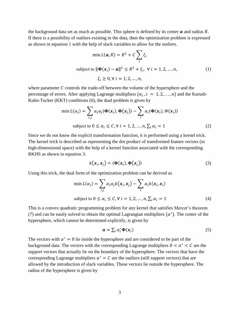
the background data set as much as possible. This sphere is defined by its center and radius .

If there is a possibility of outliers existing in the data, then the optimization problem is expressed

as shown in equation 1 with the help of slack variables to allow for the outliers.

su ect to (1)

where parameter controls the trade-off between the volume of the hypersphere and the

percentage of errors. After applying Lagrange multipliers and the Karush-

Kuhn-Tucker (KKT) conditions (6), the dual problem is given by

su ect to (2)

Since we do not know the explicit transformation function, it is performed using a kernel trick.

The kernel trick is described as representing the dot product of transformed feature vectors (in

high-dimensional space) with the help of a kernel function associated with the corresponding

RKHS as shown in equation 3.

(3)

Using this trick, the dual form of the optimization problem can be derived as

su ect to (4)

This is a convex quadratic programming problem for any kernel that satisfies Mercer’s theorem

(7) and can be easily solved to obtain the optimal Lagrangian multipliers . The center of the

hypersphere, which cannot be determined explicitly, is given by

(5)

The vectors with lie inside the hypersphere and are considered to be part of the

background data. The vectors with the corresponding Lagrange multipliers are the

support vectors that actually lie on the boundary of the hypersphere. The vectors that have the

corresponding Lagrange multipliers are the outliers (still support vectors) that are

allowed by the introduction of slack variables. These vectors lie outside the hypersphere. The

radius of the hypersphere is given by

4

(6)

where are the support vectors that lie on the boundary of the

background data set, and is the total number of support vectors. When Gaussian RBF kernel

is used with this algorithm, the SVDD method is similar to non-SVM based one-class classifier

described by Scholkopf and Smola (8). The test statistic of SVDD can then be expressed as

(7)

The test statistic basically represents the distance between the outlier (the data

sample with a Lagrange multiplier ) and the center of the hypersphere. This distance

generates a confidence level with which a data sample can be considered to be an anomaly.

An important parameter that has to be considered in the present work is , the trade-off

parameter between the volume of the hypersphere and the number of outliers allowed. As

explained by Scholkopf and Smola (8), can also be expressed as , where

represents the upper bound on the outliers permissible and also represents lower bound on the

number of support vectors that determine the boundary of the hypersphere, and is total number

of samples in the data set. The parameter can be varied based on the maximum number of

outliers being expected in a certain dataset.

3. Pedestrian Detection Using SVDD

In this report, we use the SVDD technique described in the previous section in order to perform

pedestrian detection in images. First of all, HOG-based features are extracted from overlapping

windows in an image. Each detection window forms a data sample that is used in the modeling

of the normalcy class. The permissible outliers during the modeling stage are presumably the

detection windows containing pedestrians, since the majority of the image consists of

background pixels. The confidence score of each detected outlier is given by a normalized

version of the SVDD statistic shown in equation 7. This process is repeated at different scales of

the image to account for potentially different sizes of the pedestrians in the image. Non-maximal

suppression is performed on all preliminary detections at various scales and selected the final

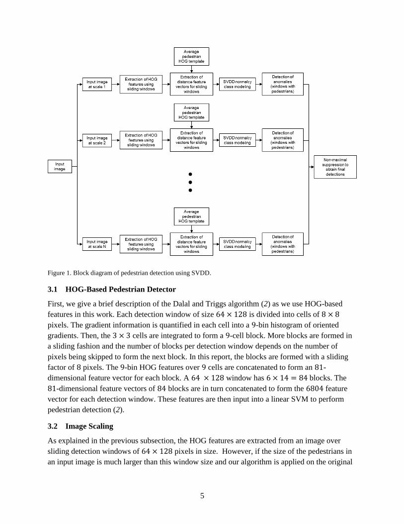
detection window based on its confidence score. The block diagram of the algorithm is

illustrated in figure 1. Each of the major steps in the algorithm is further explained in this

section.

5

Figure 1. Block diagram of pedestrian detection using SVDD.

3.1 HOG-Based Pedestrian Detector

First, we give a brief description of the Dalal and Triggs algorithm (2) as we use HOG-based

features in this work. Each detection window of size is divided into cells of

pixels. The gradient information is quantified in each cell into a -bin histogram of oriented

gradients. Then, the cells are integrated to form a -cell block. More blocks are formed in

a sliding fashion and the number of blocks per detection window depends on the number of

pixels being skipped to form the next block. In this report, the blocks are formed with a sliding

factor of pixels. The -bin HOG features over cells are concatenated to form an -

dimensional feature vector for each block. A window has blocks. The

-dimensional feature vectors of blocks are in turn concatenated to form the feature

vector for each detection window. These features are then input into a linear SVM to perform

pedestrian detection (2).

3.2 Image Scaling

As explained in the previous subsection, the HOG features are extracted from an image over

sliding detection windows of pixels in size. However, if the size of the pedestrians in

an input image is much larger than this window size and our algorithm is applied on the original

6

input image, it will not be able to detect these pedestrians. One of the options to deal with this

issue is to increase the size of the sliding detection windows. By doing so, however, there is a

need to determine and store the average pedestrian HOG template of different sizes.

Alternatively, the input image can be scaled to different sizes while keeping the size of the

detection window the same, which is equivalent to increasing the size of the detection window

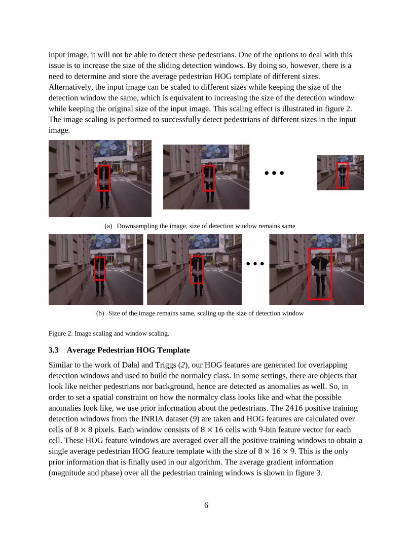
while keeping the original size of the input image. This scaling effect is illustrated in figure 2.

The image scaling is performed to successfully detect pedestrians of different sizes in the input

image.

(a) Downsampling the image, size of detection window remains same

(b) Size of the image remains same, scaling up the size of detection window

Figure 2. Image scaling and window scaling.

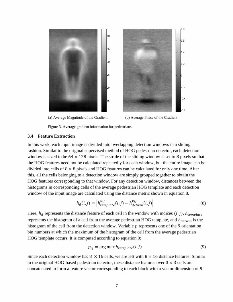
3.3 Average Pedestrian HOG Template

Similar to the work of Dalal and Triggs (2), our HOG features are generated for overlapping

detection windows and used to build the normalcy class. In some settings, there are objects that

look like neither pedestrians nor background, hence are detected as anomalies as well. So, in

order to set a spatial constraint on how the normalcy class looks like and what the possible

anomalies look like, we use prior information about the pedestrians. The positive training

detection windows from the INRIA dataset (9) are taken and HOG features are calculated over

cells of pixels. Each window consists of cells with -bin feature vector for each

cell. These HOG feature windows are averaged over all the positive training windows to obtain a

single average pedestrian HOG feature template with the size of . This is the only

prior information that is finally used in our algorithm. The average gradient information

(magnitude and phase) over all the pedestrian training windows is shown in figure 3.

7

(a) Average Magnitude of the Gradient (b) Average Phase of the Gradient

Figure 3. Average gradient information for pedestrians.

3.4 Feature Extraction

In this work, each input image is divided into overlapping detection windows in a sliding

fashion. Similar to the original supervised method of HOG pedestrian detector, each detection

window is sized to be pixels. The stride of the sliding window is set to pixels so that

the HOG features need not be calculated repeatedly for each window, but the entire image can be

divided into cells of pixels and HOG features can be calculated for only one time. After

this, all the cells belonging to a detection window are simply grouped together to obtain the

HOG features corresponding to that window. For any detection window, distances between the

histograms in corresponding cells of the average pedestrian HOG template and each detection

window of the input image are calculated using the distance metric shown in equation 8.

(8)

Here, represents the distance feature of each cell in the window with indices ,

represents the histogram of a cell from the average pedestrian HOG template, and is the

histogram of the cell from the detection window. Variable represents one of the orientation

bin numbers at which the maximum of the histogram of the cell from the average pedestrian

HOG template occurs. It is computed according to equation 9:

(9)

Since each detection window has cells, we are left with distance features. Similar

to the original HOG-based pedestrian detector, these distance features over cells are

concatenated to form a feature vector corresponding to each block with a vector dimension of .

8

The -dimensional feature vectors of 84 blocks in each window are then concatenated to form a

distance feature vector for each detection window.

3.5 SVDD Modeling

At each scale of the input image, the feature vectors from all the windows constitute the data

samples. These samples are used in equation 1 to model the image at a particular scale as a

normalcy class, while allowing certain percentage of the data samples to be outliers by setting

the value of (see section 2). Thus, all the samples that have no resemblance to pedestrians

would have similar distribution of the feature vectors and would form the normalcy class. This is

due to the fact that these samples make up the majority of the image. All the samples that

resemble the pedestrian HOG template will be modeled as outliers since the feature vectors of

these samples would be significantly different from the normalcy class.

As shown in figure 1, the SVDD modeling is performed on the input image at different scales in

order to account for the different sizes of the pedestrians. The anomalies or outliers detected

during the modeling process represent the windows containing pedestrians in them. Usually,

each pedestrian in the input image results in multiple detections due to two reasons—the HOG

features extracted from overlapping neighboring windows at a particular scale are very similar to

one another and the HOG features extracted from windows at successive scales of input image

are similar to one another. In order to merge these duplicated detections into a final detection, a

step called non-maximal suppression (NMS) is applied on the detections obtained at different

scales, as shown in figure 1.

The confidence level or score of each detection is needed to perform NMS. In this algorithm, the

SVDD test statistic shown in equation 7 is used to generate the confidence scores of the outliers.

The scores are the distances between the centers of the enclosing hyperspheres and the anomalies

obtained at different scales of the input image. The radii of the enclosing hyperspheres that are

modeled at various scales are different, and hence, the scores from equation 7 cannot be directly

compared to each other. To deal with this problem, the scores are normalized by the radii of the

hyperspheres at respective scales, as shown in equation 10. These scores represent the

confidence level of the detections with respect to the unit enclosing hypersphere and can be used

for NMS.

(10)

3.6 Non-Maximal Suppression

The final stage of the proposed unsupervised technique is NMS, which aggregates the detections

at all scales from SVDD into final detection boxes. Two NMS techniques are commonly

employed by pedestrian detection algorithms: mean shift mode estimation (2) and pairwise max

suppression (10). The mean shift method for NMS has multiple parameters to be determined,

while the pairwise max suppression has only one adjustable parameter and is very

9

computationally efficient. In this work, we used the modified pairwise max suppression

described in the addendum of the integral channel features paper by Dollar et al. (11). For a pair

of detection boxes, define a ratio as the area of the intersection between the two detection boxes

over the area of the smaller box. If this ratio exceeds a user-defined threshold, then the box with

the lower SVDD score is suppressed. Note that this modified form of pairwise max suppression

improves the interaction of two detections at nearby spatial locations but of different scales, thus

lowering the number of false alarms (11). The pairwise suppression is performed either in an

exhaustive or greedy fashion over all pairs of SVDD detections at all scales. The output of the

NMS stage is a set of final detections representation the location and scale of detected humans

within the input image.

4. Experimental Results

The proposed unsupervised pedestrian detection algorithm was tested on the INRIA dataset (9)

to illustrate its performance on a benchmark dataset. The upper limit on the number of outliers or

anomalies to be allowed at each scale in the experiment is set to of the total number of

data samples at that particular scale. There are very few data samples available at very small

scales of the input image (corresponding to very large pedestrians in the input images) to model

the enclosing hypersphere of the normalcy class. So the data samples from the smallest eight

scales of each input image are grouped together before modeling the normalcy class, and then the

anomalies (pedestrians) are obtained for these eight scales together.

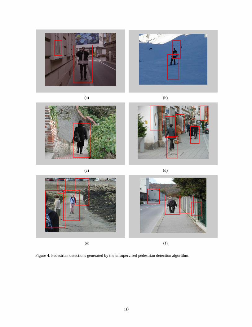
A subset of the INRIA dataset consisting of images with sizes and

are used to test the proposed algorithm. Figure 4 shows the final bounding boxes in the images

representing the pedestrian detections. As shown in this figure, the proposed algorithm is capable

of detecting pedestrians in urban and rural scenes. However, the number of false alarms appears

to be higher in urban scenes, as exemplified in figures 4a, d, and f. This observation is due to the

fact that some of the detection windows in the urban scenes have local spatial structures that are

quite different from the majority of the image. So, these windows are deemed to be anomalies

along with pedestrians. At present, the detection rate of the proposed algorithm is around at

false alarm per image. The false alarm rate will drop sharply in rural scenes with less clutter.

10

(a) (b)

(c) (d)

(e) (f)

Figure 4. Pedestrian detections generated by the unsupervised pedestrian detection algorithm.

11

5. Conclusion

In this report, we have developed an unsupervised pedestrian detection algorithm using SVDD.

The only prior information used is an average pedestrian HOG template. Using this template, a

distance feature vector is extracted for each detection window and used in normalcy class

modeling. By setting the upper limit on the number of outliers, the windows containing

pedestrians are detected as anomalies during the modeling stage. The performance of the

algorithm is demonstrated using a benchmark dataset from INRIA. Even though the algorithm

generates more false alarms compared to some supervised human detection techniques, it has

shown great potential in detecting pedestrians without any training sets. However, if a majority

part of an input image is covered by humans, the proposed algorithm will fail because the

humans are no longer outliers but becoming the normalcy class. Our future work includes

reducing the number of false alarms, as well as dealing with large number of pedestrians in an

image. Research work on different distance metrics to calculate the feature vectors will also be

performed in the near future.

12

6. References

1. Viola, P.; Jones, M. Robust Real-Time Object Detection. Proceedings of the 2nd Workshop

on Statistical and Computational Theories of Vision, 2001.

2. Dalal, N.; Triggs, B. Histogram of Oriented Gradients for Human Detection. Proceedings of

IEEE Conference of Computer Vision and Pattern Recognition, 886–893, 2005.

3. Dollar, P.; Wojek, C.; Schiele, B.; Perona, P. Pedestrian Detection: An Evaluation of the

State of the Art. IEEE Trans. on Pattern Analysis and Machine Intelligence 2012, 34 (4).

4. Dollar, P.; Belongie, S.; Perona, P. The Fastest Pedestrian Detector in the West. Proceedings

of British Machine Vision Conference, 2010.

5. Tax, D.M.J.; Duin, R.P.W. Support Vector Data Description. Machine Learning 2004, 54,

45–66.

6. Tax, D.M.J.; Duin, R.P.W. Support Vector Domain Description. Pattern Recognition Letters

1999, 20, 1191–1199.

7. Vapnik, V. N. Statistical Learning Theory; John Wiley and Sons, New York, 1998.

8. Scholkopf, B.; Smola, A. J. Learning with Kernels; The MIT Press, Massachusetts, 2002.

9. Dalal, N. INRIA Person Dataset. http://pascal.inrialpes.fr/data/human/ (accessed June, 2012).

10. Felzenszwalb, P.; McAllester, D.; Ramanan, D. A Discriminatively Trained, Multiscale,

Deformable Part Model. Proceedings of IEEE Conference of Computer Vision and Pattern

Recognition, 2008.

11. Dollar, P.; Tu, Z.; Perona, P.; Belongie, S. Integral Channel Features. Proceedings of British

Machine Vision Conference, 2009.

13

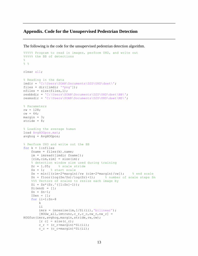
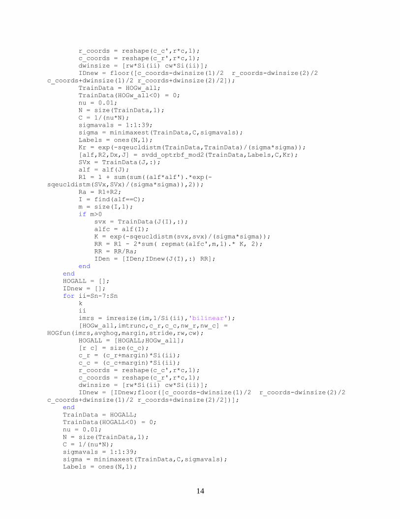
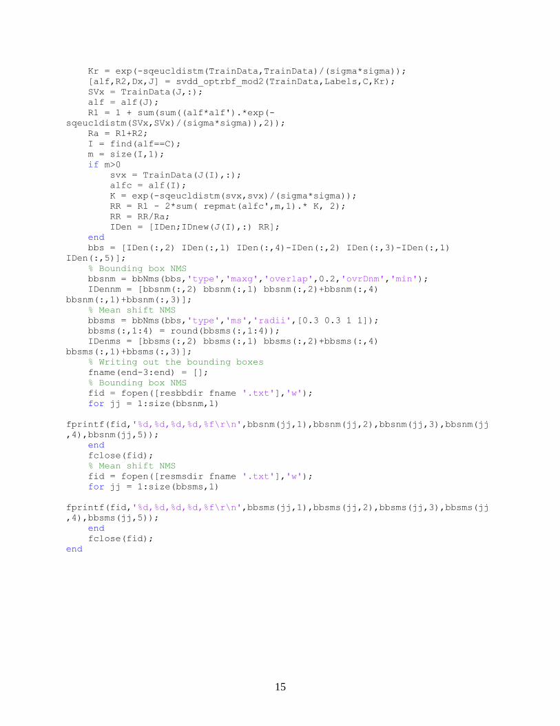
Appendix. Code for the Unsupervised Pedestrian Detection

The following is the code for the unsupervised pedestrian detection algorithm.

%%%%% Program to read in images, perform UHD, and write out %%%%% the BB of detections % % %

clear all;

% Reading in the data imdir = 'C:\Users\SOAR\Documents\D2D\UHD\dset\'; files = dir([imdir '*png']); nfiles = size(files,1); resbbdir = 'C:\Users\SOAR\Documents\D2D\UHD\dset\BB\'; resmsdir = 'C:\Users\SOAR\Documents\D2D\UHD\dset\MS\';

% Parameters rw = 128; cw = 64; margin = 3; stride = 8;

% Loading the average human load AvgHOGpos.mat; avghog = AvgHOGpos;

% Perform UHD and write out the BB for k = 1:nfiles fname = files(k).name; im = imread([imdir fname]); [rim,cim,zim] = size(im); % detection window size used during training Sr = 1.05; % scale stride Ss = 1; % start scale Se = min([(rim-2*margin)/rw (cim-2*margin)/cw]); % end scale Sn = floor(log(Se/Ss)/log(Sr)+1); % number of scale steps Sn %%% Vectors of scales to resize each image by Si = Ss*(Sr.^([1:Sn]-1)); Si(end) = []; Sn = Sn-1; IDen = []; for ii=1:Sn-8 k ii imrs = imresize(im,1/Si(ii),'bilinear'); [HOGw_all,imtrunc,c_r,c_c,nw_r,nw_c] =

HOGfun(imrs,avghog,margin,stride,rw,cw); [r c] = size(c_c); c_r = (c_r+margin)*Si(ii); c_c = (c_c+margin)*Si(ii);

14

r_coords = reshape(c_c',r*c,1); c_coords = reshape(c_r',r*c,1); dwinsize = [rw*Si(ii) cw*Si(ii)]; IDnew = floor([c_coords-dwinsize(1)/2 r_coords-dwinsize(2)/2

c_coords+dwinsize(1)/2 r_coords+dwinsize(2)/2]); TrainData = HOGw_all; TrainData(HOGw_all<0) = 0; nu = 0.01; N = size(TrainData,1); C = 1/(nu*N); sigmavals = 1:1:39; sigma = minimaxest(TrainData,C,sigmavals); Labels = ones(N,1); Kr = exp(-sqeucldistm(TrainData,TrainData)/(sigma*sigma)); [alf,R2,Dx,J] = svdd_optrbf_mod2(TrainData,Labels,C,Kr); SVx = TrainData(J,:); alf = alf(J); R1 = 1 + sum(sum((alf*alf').*exp(-

sqeucldistm(SVx,SVx)/(sigma*sigma)),2)); Ra = R1+R2; I = find(alf==C); m = size(I,1); if m>0 svx = TrainData(J(I),:); alfc = alf(I); K = exp(-sqeucldistm(svx,svx)/(sigma*sigma)); RR = R1 - 2*sum( repmat(alfc',m,1).* K, 2); RR = RR/Ra; IDen = [IDen;IDnew(J(I),:) RR]; end end HOGALL = []; IDnew = []; for ii=Sn-7:Sn k ii imrs = imresize(im,1/Si(ii),'bilinear'); [HOGw_all,imtrunc,c_r,c_c,nw_r,nw_c] =

HOGfun(imrs,avghog,margin,stride,rw,cw); HOGALL = [HOGALL;HOGw_all]; [r c] = size(c_c); c_r = (c_r+margin)*Si(ii); c_c = (c_c+margin)*Si(ii); r_coords = reshape(c_c',r*c,1); c_coords = reshape(c_r',r*c,1); dwinsize = [rw*Si(ii) cw*Si(ii)]; IDnew = [IDnew;floor([c_coords-dwinsize(1)/2 r_coords-dwinsize(2)/2

c_coords+dwinsize(1)/2 r_coords+dwinsize(2)/2])]; end TrainData = HOGALL; TrainData(HOGALL<0) = 0; nu = 0.01; N = size(TrainData,1); C = 1/(nu*N); sigmavals = 1:1:39; sigma = minimaxest(TrainData,C,sigmavals); Labels = ones(N,1);

15

Kr = exp(-sqeucldistm(TrainData,TrainData)/(sigma*sigma)); [alf,R2,Dx,J] = svdd_optrbf_mod2(TrainData,Labels,C,Kr); SVx = TrainData(J,:); alf = alf(J); R1 = 1 + sum(sum((alf*alf').*exp(-

sqeucldistm(SVx,SVx)/(sigma*sigma)),2)); Ra = R1+R2; I = find(alf==C); m = size(I,1); if m>0 svx = TrainData(J(I),:); alfc = alf(I); K = exp(-sqeucldistm(svx,svx)/(sigma*sigma)); RR = R1 - 2*sum( repmat(alfc',m,1).* K, 2); RR = RR/Ra; IDen = [IDen;IDnew(J(I),:) RR]; end bbs = [IDen(:,2) IDen(:,1) IDen(:,4)-IDen(:,2) IDen(:,3)-IDen(:,1)

IDen(:,5)]; % Bounding box NMS bbsnm = bbNms(bbs,'type','maxg','overlap',0.2,'ovrDnm','min'); IDennm = [bbsnm(:,2) bbsnm(:,1) bbsnm(:,2)+bbsnm(:,4)

bbsnm(:,1)+bbsnm(:,3)]; % Mean shift NMS bbsms = bbNms(bbs,'type','ms','radii',[0.3 0.3 1 1]); bbsms(:,1:4) = round(bbsms(:,1:4)); IDenms = [bbsms(:,2) bbsms(:,1) bbsms(:,2)+bbsms(:,4)

bbsms(:,1)+bbsms(:,3)]; % Writing out the bounding boxes fname(end-3:end) = []; % Bounding box NMS fid = fopen([resbbdir fname '.txt'],'w'); for jj = 1:size(bbsnm,1)

fprintf(fid,'%d,%d,%d,%d,%f\r\n',bbsnm(jj,1),bbsnm(jj,2),bbsnm(jj,3),bbsnm(jj

,4),bbsnm(jj,5)); end fclose(fid); % Mean shift NMS fid = fopen([resmsdir fname '.txt'],'w'); for jj = 1:size(bbsms,1)

fprintf(fid,'%d,%d,%d,%d,%f\r\n',bbsms(jj,1),bbsms(jj,2),bbsms(jj,3),bbsms(jj

,4),bbsms(jj,5)); end fclose(fid); end

16

NO. OF

COPIES ORGANIZATION 1 ADMNSTR

(PDF) DEFNS TECHL INFO CTR

ATTN DTIC OCP 1 GOVT PRINTG OFC

(PDF) A MALHOTRA

4 US ARMY CERDEC NVESD

(PDFS) ATTN L GRACEFFO

ATTN M GROENERT

ATTN J HILGER

ATTN J WRIGHT 2 US ARMY AMRDEC

(PDFS) ATTN RDMR WDG I J MILLS

ATTN RDMR WDG S D WAAGEN 2 US ARMY RSRCH OFFICE

(PDFS) ATTN RDRL ROI C L DAI

ATTN RDRL ROI M J LAVERY 18 US ARMY RSRCH LAB

(PDFS) ATTN IMAL HRA MAIL & RECORDS MGMT

ATTN RDRL CIO LL TECHL LIB

ATTN RDRL SE P PERCONTI

ATTN RDRL SES J EICKE

ATTN RDRL SES M D’ONOFRIO

ATTN RDRL SES N NASRABADI

ATTN RDRL SES E R RAO

ATTN RDRL SES E A CHAN

ATTN RDRL SES E H KWON

ATTN RDRL SES E S YOUNG

ATTN RDRL SES E J DAMMANN

ATTN RDRL SES E D ROSARIO

ATTN RDRL SES E H BRANDT

ATTN RDRL SES E S HU

ATTN RDRL SES E M THIELKE

ATTN RDRL SES E P RAUSS

ATTN RDRL SES E P GURRAM

ATTN RDRL SES E C REALE