Unsupervised Machine Learning on a Hybrid Quantum Computer

J. S. Otterbach, R. Manenti, N. Alidoust, A. Bestwick, M. Block, B. Bloom, S. Caldwell, N. Didier, E.

Schuyler Fried, S. Hong, P. Karalekas, C. B. Osborn, A. Papageorge, E. C. Peterson, G. Prawiroatmodjo,

N. Rubin, Colm A. Ryan, D. Scarabelli, M. Scheer, E. A. Sete, P. Sivarajah, Robert S. Smith, A. Staley,

N. Tezak, W. J. Zeng, A. Hudson, Blake R. Johnson, M. Reagor, M. P. da Silva, and C. RigettiRigetti Computing, Inc., Berkeley, CA

(Dated: December 18, 2017)

Machine learning techniques have led to broad adoption of a statistical model of computing. Thestatistical distributions natively available on quantum processors are a superset of those availableclassically. Harnessing this attribute has the potential to accelerate or otherwise improve machinelearning relative to purely classical performance. A key challenge toward that goal is learningto hybridize classical computing resources and traditional learning techniques with the emergingcapabilities of general purpose quantum processors. Here, we demonstrate such hybridization bytraining a 19-qubit gate model processor to solve a clustering problem, a foundational challengein unsupervised learning. We use the quantum approximate optimization algorithm in conjunctionwith a gradient-free Bayesian optimization to train the quantum machine. This quantum/classicalhybrid algorithm shows robustness to realistic noise, and we find evidence that classical optimizationcan be used to train around both coherent and incoherent imperfections.

INTRODUCTION

The immense power of quantum computation is illus-trated by flagship quantum algorithms that solve problemssuch as factoring [1] and linear systems of equations [2],amongst many others, much more efficiently than classicalcomputers. The building of a quantum device with errorrates well below the fault-tolerance threshold [3–6] poses achallenge to the implementation of these kinds of quantumalgorithms on near-term devices. In recent years severalnew algorithms targeting these near-term devices havebeen proposed. These algorithms focus on short-depthparameterized quantum circuits, and use quantum com-putation as a subroutine embedded in a larger classicaloptimization loop. It has been shown that optimizing theperformance of the quantum subroutine—by varying a fewfree parameters—allows for calculating binding energiesin quantum chemistry [7–10], as well as solving some com-binatorial [11, 12] and tensor network problems [13]. Inthis paper we choose to focus on an unsupervised machinelearning task known as clustering, which we translate intoa combinatorial optimization problem [14, 15] that canbe solved by the quantum approximate optimization algo-rithm (QAOA) [11, 12]. We implement said algorithm ona 19-qubit computer using a flexible quantum program-ming platform [16, 17]. We show that our implementationof this algorithm finds the optimal solution to randomproblem instances with high probability, and that goodapproximate solutions are found in all investigated cases,even with relatively noisy gates. This robustness is en-abled partially by using a Bayesian procedure [18, 19] inthe classical optimization loop for the quantum circuitparameters.

CLUSTERING

The particular unsupervised machine learning problemwe focus on here is known as clustering [20, 21]. Clusteringconsists of assigning labels to elements of a dataset basedonly on how similar they are to each other—like objectswill have the same label, unlike objects will have differentlabels. Mathematically, the dataset D has elements xifor 1 ≤ i ≤ n, where each element is a k-dimensionalfeature vector (a numerical representation of any object ofinterest: a photograph, an audio recording, etc.). In orderto represent dissimilarity, we need to define a distancemeasure d(xi,xj) between two samples xi and xj . Afamiliar choice for a distance measure is the Euclideandistance, but specific applications may naturally lead tovery different choices for the metric and the distance [22,23].

Most common choices of distances allows us to calcu-late a matrix of distances between all points in O(kn2)steps, by simply calculating the distance between everypossible pair of data samples. Let this matrix be de-noted by C where Cij = d(xi,xj). This matrix can beinterpreted as an adjacency matrix of a graph G, whereeach vertex represents an element of D and Cij is theweight of edge between vertices i and j. In general thematrix C will be dense leading to a fully connected graphon n vertices, but different choices of distance metricsalong with coarse-graining can make this distance matrixsparse. In clustering, the main assumption is that distantpoints belong to different clusters; hence maximizing theoverall sum of all weights (distances) between nodes withdifferent labels represents a natural clustering algorithm.The mathematical formulation of this is a Maximum-Cut(Maxcut) problem [15], defined as Maxcut(G,C) forthe dense graph G of the distance matrix C.

More precisely, the Maxcut problem consists of an

arX

iv:1

712.

0577

1v1

[qu

ant-

ph]

15

Dec

201

7

undirected graph G = (V,E) with a set of vertices V anda set of edges E between those vertices. The weight wij ofan edge between vertices i and j is a positive real number,with wij = 0 if there is no edge between them. A cutδ(S) ⊂ E is a set of edges that separates the vertices Vinto two disjoint sets S and S = V \ S. The cost w(δ(S))of a cut is defined as the sum of all weights of edgesconnecting vertices in S with vertices in S

w(δ(S)) =∑

i∈S,j∈S

wij . (1)

The problem Maxcut(G,w) is now easily formulated asan optimization objective

Maxcut(G,w) = maxS⊂V

w(δ(S)). (2)

The Maxcut problem is an example of the classof NP-complete problems [24], which are notoriouslyhard to solve. Many other combinatorial problems canbe reduced to Maxcut—e.g., machine scheduling [25],computer-aided design [26], traffic message managementproblems [27], image recognition [28], quadratic uncon-strained optimization problems (QUBO) [15] and manymore. One approach to solving Maxcut is to construct aphysical system—typically a set of interacting spin- 1

2 par-ticles [14]—whose lowest energy state encodes the solutionto the problem, so that solving the problem is equivalentto finding the ground state of the system [29]. This is theapproach we take here.

QUANTUM APPROXIMATE OPTIMIZATIONALGORITHM

It is possible to find the ground state of interactingspin systems using an algorithm known as the quantumapproximate optimization algorithm (QAOA) [11]. QAOAcan be thought of as a heuristic to prepare a superpo-sition of bit strings with probability amplitudes heavilyconcentrated around the solution. The encoding of theproblem itself is given by a cost Hamiltonian (cf. S1)

HC = −1

2

∑i,j

Cij(1− σzi σzj ), (3)

and QAOA approximates the ground state by initiallypreparing the equal superposition of all bit strings, theniteratively applying a pair of unitary operations beforemeasuring (see Fig. 1). For the ith iteration, we evolvethe system with cost unitary Ui = exp(−iγiHC) for someangle γi, followed by the driver unitary Vi = exp(−iβiHD)for some angle βi, where the driver Hamiltonian is

HD =∑i

σxi . (4)

Bayesianoptimizer

cluster

assignments

(bit strings)

Measu

re

Dri

ver

un

itary

Cost unitary

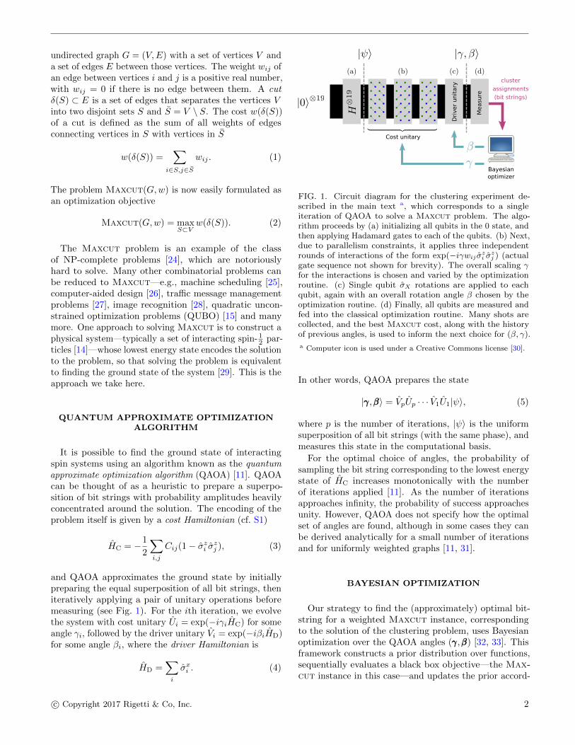
FIG. 1. Circuit diagram for the clustering experiment de-scribed in the main text a, which corresponds to a singleiteration of QAOA to solve a Maxcut problem. The algo-rithm proceeds by (a) initializing all qubits in the 0 state, andthen applying Hadamard gates to each of the qubits. (b) Next,due to parallelism constraints, it applies three independentrounds of interactions of the form exp(−iγwij σzi σzj ) (actualgate sequence not shown for brevity). The overall scaling γfor the interactions is chosen and varied by the optimizationroutine. (c) Single qubit σX rotations are applied to eachqubit, again with an overall rotation angle β chosen by theoptimization routine. (d) Finally, all qubits are measured andfed into the classical optimization routine. Many shots arecollected, and the best Maxcut cost, along with the historyof previous angles, is used to inform the next choice for (β, γ).

a Computer icon is used under a Creative Commons license [30].

In other words, QAOA prepares the state

|γγγ,βββ〉 = VpUp · · · V1U1|ψ〉, (5)

where p is the number of iterations, |ψ〉 is the uniformsuperposition of all bit strings (with the same phase), andmeasures this state in the computational basis.

For the optimal choice of angles, the probability ofsampling the bit string corresponding to the lowest energystate of HC increases monotonically with the numberof iterations applied [11]. As the number of iterationsapproaches infinity, the probability of success approachesunity. However, QAOA does not specify how the optimalset of angles are found, although in some cases they canbe derived analytically for a small number of iterationsand for uniformly weighted graphs [11, 31].

BAYESIAN OPTIMIZATION

Our strategy to find the (approximately) optimal bit-string for a weighted Maxcut instance, correspondingto the solution of the clustering problem, uses Bayesianoptimization over the QAOA angles (γγγ,βββ) [32, 33]. Thisframework constructs a prior distribution over functions,sequentially evaluates a black box objective—the Max-cut instance in this case—and updates the prior accord-

c© Copyright 2017 Rigetti & Co, Inc. 2

0 1 2 4

10 11 12 13 14

5 6 7 8 9

15 16 17 18 19

a

b

30 1 2 4

10 11 12 13 14

5 6 7 8 9

15 16 17 18 19

a 3

2 mm

1 m

FIG. 2. Connectivity of Rigetti 19Q. a, Chip schematicshowing tunable transmons (teal circles) capacitively coupledto fixed-frequency transmons (pink circles). b, Optical chipimage. Note that some couplers have been dropped to producea lattice with three-fold, rather than four-fold, connectivity.

ing to Bayes’ rule

p(f |y) ∼ p(y|f)p(f), (6)

where p(f |y) is the posterior distribution over functionspace given the observations y, p(f) is the prior overfunction space, and p(y|f) is the likelihood of observingthe values y given the model for f . With growing numberof optimization steps (observations y) the true black-boxobjective is increasingly well approximated. The trick liesin choosing the prior p(f) in a way that offers closed-formsolutions for easy numerical updates, such as Gaussianprocesses, which assume a normal distribution as a priorover the function space [18](cf. S10). In the present caseof QAOA, it should be noted that sampling at each stepwill generally lead to a non-trivial distribution of valueswhen the state |γγγ,βββ〉 is entangled or mixed. To fit thisinto the Bayesian Optimization framework we calculatethe best observed sample and return this to the optimizer.Hence, the function f represents the value of the bestsampled bit string at location γγγ,βββ. More generally, onecould compute any statistic of the distribution (as detailed

in the appendix).To avoid a random walk over the space of potential

evaluation points, the Bayesian optimizer maximizes autility function that can be calculated from the posteriordistribution after each update. In this way, it intelligentlychooses points to minimize the number of costly evalua-tions of the black box objective function (see the appendixfor more details).

THE QUANTUM PROCESSOR

We ran the QAOA optimizer on a quantum processorconsisting of 20 superconducting transmon qubits [34]with fixed capacitive coupling in the lattice shown inFig. 2. Qubits 0–4 and 10–14 are tunable while qubits5–9 and 15–19 are fixed-frequency devices. The formerhave two Josephson junctions in an asymmetric SQUIDgeometry to provide roughly 1 GHz of frequency tunability,and flux-insensitive “sweet spots” [35] near ωmax

01 /2π ≈4.5 GHz and ωmin

01 /2π ≈ 3.0 GHz. These tunable qubitsare coupled to bias lines for AC and DC flux delivery. Eachqubit is capacitively coupled to a quasi-lumped elementresonator for dispersive readout of the qubit state [36, 37].Single-qubit control is effected by applying microwavedrives at the resonator ports, and two-qubit gates areactivated via RF drives on the flux bias lines, describedbelow.

The device is fabricated on a high-resistivity siliconsubstrate with superconducting through-silicon via tech-nology [38] to improve RF-isolation. The superconductingcircuitry is realized with Aluminum (Tc ≈ 1.2 K), andpatterned using a combination of optical and electron-beam lithography. Due to a fabrication defect, qubit 3is not tunable, which prohibits operation of the 2-qubitparametric gate described below between qubits 3 andits neighbors (8 and 9). Consequently, we treat this as a19-qubit processor.

In Rigetti 19Q, as we call our device, each tunable qubitis capacitively coupled to one-to-three fixed-frequencyqubits. The DC flux biases are set close to zero fluxsuch that each tunable qubit is at its maximum frequencyωmax

T . Two-qubit parametric CZ gates are activated in the|11〉 ↔ |20〉 and/or |11〉 ↔ |02〉 sub-manifolds by applyingan RF flux pulse with amplitude A0, frequency ωm andduration tCZ to the tunable qubit [39–41]. For RF fluxmodulation about the qubit extremal frequency, the oscil-lation frequency is doubled to 2ωm and the mean effectivequbit frequency shifts to ωT. Note that the frequencyshift increases with larger flux pulse amplitude. Theeffective detuning between neighboring qubits becomes∆ = ωT − ωF.

The resonant condition for a CZ gate is achieved when∆ = 2ωm− ηT or ∆ = 2ωm + ηF, where ηT, ηF are the an-harmonicities of the tunable and fixed qubit, respectively.An effective rotation angle of 2π on these transitions im-

c© Copyright 2017 Rigetti & Co, Inc. 3

5 6

15 17

0 1 2 4

10 11 12 13 14

5 6 7 8 9

15 16 17 18 19

0 1 2 4

10 11 12 13 14

5 6 7 8 9

15 16 17 18 19

0 1 2 4

10 11 12 13 14

5 6 7 8 9

15 16 17 18 19

0.18

0.59 0.

56

0.40 0.

570.71 0.

72

0.43

0.29

0.230.64

0.600.36

0.52

0.490.44

0.63

0.410.50

0.400.81

a

b

FIG. 3. a, The general form of the clustering problem instancesolved on the 19Q chip, and b, the corresponding Maxcutproblem instance solved on the 19 qubit chip. The edgeweights—corresponding to the overlap between neighbouringprobability distributions on the plane—are chosen at randomand the labels indicate the mapping to the correspondingqubit. The vertices are colored according to the solution tothe problem.

FIG. 4. Traces for the normalized Maxcut cost for 83 inde-pendent runs of the algorithm on the 19Q chip for the fixed,but random, problem instances of Fig. 3. Notice that mosttraces reach the optimal value of 1 well before the cutoff at 55steps.

parts a minus sign to the |11〉 state, implementing aneffective CZ gate. The time-scale of these entanglinggates is in the range 100–250 ns. Due to finite bandwidthconstraints of our control electronics, the applied fluxpulse is shaped as a square pulse with linear rise and falltime of 30 ns.

FIG. 5. The performance of our implementation of the cluster-ing algorithm on the 19Q chip (blue) and a noiseless simulationthrough the Forest [42] quantum virtual machine (orange) canbe compared to the performance of an algorithm that simplydraws cluster assignments at random (red: Theoretical curve,green: empirical confirmation). It is clear that out algorithmgenerates the optimal assignment much more quickly thanit would be expected by chance: the 95% confidence regionfor our empirical observations have very small overlap for thedistribution given by random assignments. See appendix formore detailed statistics.

IMPLEMENTATION

We demonstrate the implementation of the proposedclustering algorithm on a problem with a cost Hamilto-nian constructed to match the connectivity of Rigetti 19Q.Such a choice minimizes the circuit depth required forthe algorithm while utilizing all available qubits. Thisproblem corresponds to clustering an arrangement of over-lapping probability distributions, whose dissimilarity isgiven by the Bhattacharyya coefficient [43]—a measure fordistributional overlap. A cartoon of such an arrangement,and the corresponding graph for the weighted Maxcutproblem, is depicted in Fig. 3 [44]. This problem is solvedusing a single iteration (p = 1) of QAOA, and using upto 55 steps of a Bayesian optimizer to choose the angles(γ, β). This procedure is repeated several times to gatherstatistics about the number of steps necessary to reachthe optimal answer.

Using the available interactions and local gate oper-ations, we are able to implement the cost unitary in acircuit of depth corresponding to six CZ gates interspersedwith single qubit operations and hence fitting well withina single coherence time of the qubits. This circuit depthis dictated by two independent factors. The first is theimplementation of the cost unitary. Since all the terms inthe cost Hamiltonian commute, it is possible to decomposethe cost unitary into a separate unitary for each cost term.These cost terms, in turn, take the form exp(−iγwij σzi σzj )that does not directly correspond to one of the nativegates in our quantum computer. However, they can be

c© Copyright 2017 Rigetti & Co, Inc. 4

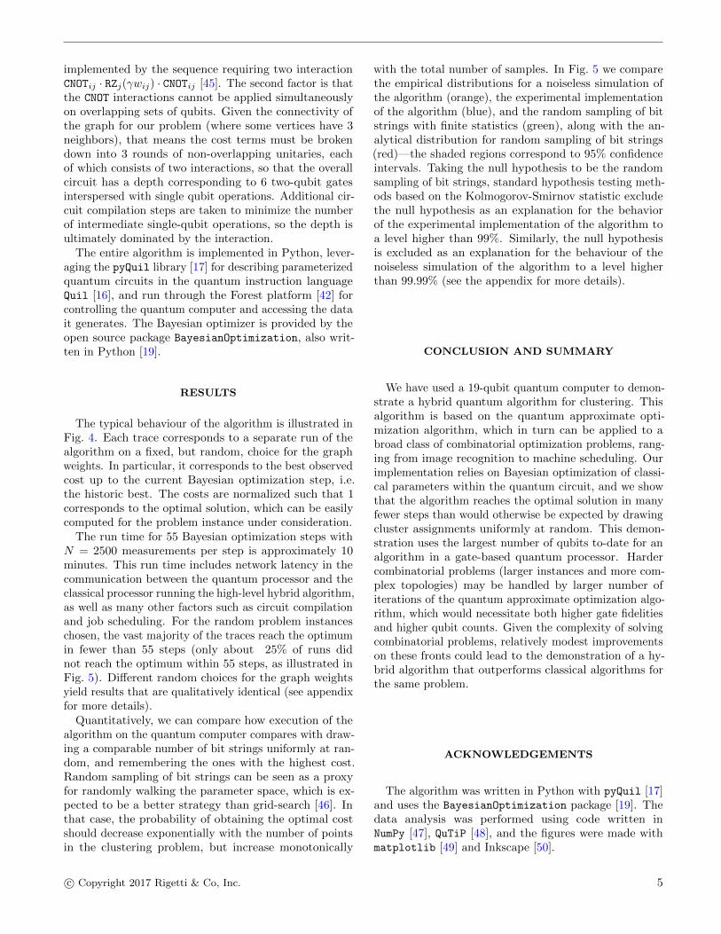
implemented by the sequence requiring two interactionCNOTij · RZj(γwij) · CNOTij [45]. The second factor is thatthe CNOT interactions cannot be applied simultaneouslyon overlapping sets of qubits. Given the connectivity ofthe graph for our problem (where some vertices have 3neighbors), that means the cost terms must be brokendown into 3 rounds of non-overlapping unitaries, eachof which consists of two interactions, so that the overallcircuit has a depth corresponding to 6 two-qubit gatesinterspersed with single qubit operations. Additional cir-cuit compilation steps are taken to minimize the numberof intermediate single-qubit operations, so the depth isultimately dominated by the interaction.

The entire algorithm is implemented in Python, lever-aging the pyQuil library [17] for describing parameterizedquantum circuits in the quantum instruction languageQuil [16], and run through the Forest platform [42] forcontrolling the quantum computer and accessing the datait generates. The Bayesian optimizer is provided by theopen source package BayesianOptimization, also writ-ten in Python [19].

RESULTS

The typical behaviour of the algorithm is illustrated inFig. 4. Each trace corresponds to a separate run of thealgorithm on a fixed, but random, choice for the graphweights. In particular, it corresponds to the best observedcost up to the current Bayesian optimization step, i.e.the historic best. The costs are normalized such that 1corresponds to the optimal solution, which can be easilycomputed for the problem instance under consideration.

The run time for 55 Bayesian optimization steps withN = 2500 measurements per step is approximately 10minutes. This run time includes network latency in thecommunication between the quantum processor and theclassical processor running the high-level hybrid algorithm,as well as many other factors such as circuit compilationand job scheduling. For the random problem instanceschosen, the vast majority of the traces reach the optimumin fewer than 55 steps (only about 25% of runs didnot reach the optimum within 55 steps, as illustrated inFig. 5). Different random choices for the graph weightsyield results that are qualitatively identical (see appendixfor more details).

Quantitatively, we can compare how execution of thealgorithm on the quantum computer compares with draw-ing a comparable number of bit strings uniformly at ran-dom, and remembering the ones with the highest cost.Random sampling of bit strings can be seen as a proxyfor randomly walking the parameter space, which is ex-pected to be a better strategy than grid-search [46]. Inthat case, the probability of obtaining the optimal costshould decrease exponentially with the number of pointsin the clustering problem, but increase monotonically

with the total number of samples. In Fig. 5 we comparethe empirical distributions for a noiseless simulation ofthe algorithm (orange), the experimental implementationof the algorithm (blue), and the random sampling of bitstrings with finite statistics (green), along with the an-alytical distribution for random sampling of bit strings(red)—the shaded regions correspond to 95% confidenceintervals. Taking the null hypothesis to be the randomsampling of bit strings, standard hypothesis testing meth-ods based on the Kolmogorov-Smirnov statistic excludethe null hypothesis as an explanation for the behaviorof the experimental implementation of the algorithm toa level higher than 99%. Similarly, the null hypothesisis excluded as an explanation for the behaviour of thenoiseless simulation of the algorithm to a level higherthan 99.99% (see the appendix for more details).

CONCLUSION AND SUMMARY

We have used a 19-qubit quantum computer to demon-strate a hybrid quantum algorithm for clustering. Thisalgorithm is based on the quantum approximate opti-mization algorithm, which in turn can be applied to abroad class of combinatorial optimization problems, rang-ing from image recognition to machine scheduling. Ourimplementation relies on Bayesian optimization of classi-cal parameters within the quantum circuit, and we showthat the algorithm reaches the optimal solution in manyfewer steps than would otherwise be expected by drawingcluster assignments uniformly at random. This demon-stration uses the largest number of qubits to-date for analgorithm in a gate-based quantum processor. Hardercombinatorial problems (larger instances and more com-plex topologies) may be handled by larger number ofiterations of the quantum approximate optimization algo-rithm, which would necessitate both higher gate fidelitiesand higher qubit counts. Given the complexity of solvingcombinatorial problems, relatively modest improvementson these fronts could lead to the demonstration of a hy-brid algorithm that outperforms classical algorithms forthe same problem.

ACKNOWLEDGEMENTS

The algorithm was written in Python with pyQuil [17]and uses the BayesianOptimization package [19]. Thedata analysis was performed using code written inNumPy [47], QuTiP [48], and the figures were made withmatplotlib [49] and Inkscape [50].

c© Copyright 2017 Rigetti & Co, Inc. 5

CONTRIBUTIONS

J.S.O., N.R., and M.P.S. developed the theoretical pro-posal. J.S.O. and E.S.F. implemented the algorithm,and J.S.O. performed the data analysis. M.B., E.A.S.,M.S., and A.B. designed the 20-qubit device. R.M., S.C.,C.A.R., N.A., A.S., S.H., N.D., D.S., and P.S. broughtup the experiment. C.B.O., A.P., B.B., P.K., G.P.,N.T., M.R. developed the infrastructure for automatic re-calibration. E.C.P., P.K., W.Z., and R.S.S. developed thecompiler and QVM tools. J.S.O., M.P.S., B.R.J., M.R.,R.M. wrote the manuscript. B.R.J., M.R., A.H., M.P.S.,and C.R. were principal investigators of the effort.

[1] P. W. Shor, in Proceedings 35th Annual Symposium onFoundations of Computer Science (1994) pp. 124–134.

[2] A. W. Harrow, A. Hassidim, and S. Lloyd, Phys. Rev.Lett. 103, 150502 (2009).

[3] P. W. Shor, in Proceedings of 37th Conference on Foun-dations of Computer Science (1996) pp. 56–65.

[4] E. Knill, R. Laflamme, and W. H.Zurek, Science 279, 342 (1998),http://science.sciencemag.org/content/279/5349/342.full.pdf.

[5] D. Aharonov and M. Ben-Or, SIAMJournal on Computing 38, 1207 (2008),https://doi.org/10.1137/S0097539799359385.

[6] P. Aliferis, D. Gottesman, and J. Preskill, Quantum Info.Comput. 6, 97 (2006).

[7] A. Peruzzo, J. McClean, P. Shadbolt, M.-H. Yung, X.-Q.Zhou, P. J. Love, A. Aspuru-Guzik, and J. L. O’Brien,Nature Communications 5, 4213 EP (2014).

[8] J. R. McClean, J. Romero, R. Babbush, and A. Aspuru-Guzik, New Journal of Physics 18, 023023 (2016).

[9] A. Kandala, A. Mezzacapo, K. Temme, M. Takita,M. Brink, J. M. Chow, and J. M. Gambetta, Nature549, 242 EP (2017).

[10] J. I. Colless, V. V. Ramasesh, D. Dahlen, M. S. Blok,J. R. McClean, J. Carter, W. A. de Jong, and I. Siddiqi,“Robust determination of molecular spectra on a quantumprocessor,” (2017), arXiv:1707.06408.

[11] E. Farhi, J. Goldstone, and S. Gutmann, arXiv:1411.4028(2014).

[12] S. Hadfield, Z. Wang, B. O’Gorman, E. G. Rieffel, D. Ven-turelli, and R. Biswas, “From the quantum approximateoptimization algorithm to a quantum alternating operatoransatz,” (2017), arXiv:1709.03489.

[13] I. H. Kim and B. Swingle, “Robust entanglement renor-malization on a noisy quantum computer,” (2017),arXiv:1711.07500.

[14] A. Lucas, Frontiers in Physics 2, 5 (2014).[15] S. Poljak and Z. Tuza, in Combinatorial Optimization,

Vol. 20, edited by W. Cook, L. Lovasz, and P. Seymour(American Mathematical Society, 1995).

[16] R. S. Smith, M. J. Curtis, and W. J. Zeng, “A practicalquantum instruction set architecture,” (2016).

[17] Rigetti Computing, “pyquil,”https://github.com/rigetticomputing/pyquil (2016).

[18] C. E. Rasmussen and C. K. I. Williams, Gaussian Pro-cesses for Machine Learning (MIT Press, 2006).

[19] F. Nogueira, “bayesian-optimization,”https://github.com/fmfn/BayesianOptimization (2014).

[20] A. K. Jain, M. N. Murty, and P. J. Flynn, ACM Comput.Surv. 31, 264 (1999).

[21] A. K. Jain and R. C. Dubes, Algorithms for ClusteringData (Prentice-Hall, Inc., Upper Saddle River, NJ, USA,1988).

[22] A. S. Shirkhorshidi, S. Aghabozorgi, and T. Y. Wah,PLOS ONE 10, 1 (2015).

[23] S. Boriah, V. Chandola, and V. Kumar, “Similar-ity measures for categorical data: A comparativeevaluation,” in Proceedings of the 2008 SIAM In-ternational Conference on Data Mining , pp. 243–254,http://epubs.siam.org/doi/pdf/10.1137/1.9781611972788.22.

[24] R. M. Karp, in Complexity of Computer Computations,edited by R. E. Miller and J. W. Thatcher (New York:Plenum, 1972) pp. 85–103.

[25] B. Alidaee, G. A. Kochenberger, and A. Ahmadian,International Journal of Systems Science 25, 401 (1994).

[26] J. Krarup and P. M. Pruzan, “Computer-aided layoutdesign,” in Mathematical Programming in Use, editedby M. L. Balinski and C. Lemarechal (Springer BerlinHeidelberg, Berlin, Heidelberg, 1978) pp. 75–94.

[27] G. Gallo, P. L. Hammer, and B. Simeone, “Quadraticknapsack problems,” in Combinatorial Optimization,edited by M. W. Padberg (Springer Berlin Heidelberg,Berlin, Heidelberg, 1980) pp. 132–149.

[28] H. Neven, G. Rose, and W. G. Macready, arXiv:0804.4457(2008).

[29] Note that we can turn any maximization procedure intoa minimization procedure by simply changing the sign ofthe objective function.

[30] GNOME icon artists, “gnome computer icon,” (2008),creative commons license.

[31] Z. Wang, S. Hadfield, Z. Jiang, and E. G. Rieffel, “Thequantum approximation optimization algorithm for max-cut: A fermionic view,” (2017).

[32] B. Shahriari, K. Swersky, Z. Wang, R. P. Adams, andN. de Freitas, Proceedings of the IEEE 104, 148 (2015).

[33] J. Snoek, O. Rippel, K. Swersky, R. Kiros, N. Satish,N. Sundaram, M. M. A. Patwary, P. Prabhat, and R. P.Adams, in Proceedings of the 32Nd International Confer-ence on International Conference on Machine Learning -Volume 37 , ICML’15 (JMLR.org, 2015) pp. 2171–2180.

[34] J. Koch, T. Yu, J. M. Gambetta, A. A. Houck, D. I.Schuster, J. Majer, A. Blais, M. H. Devoret, S. M. Girvin,and R. J. Schoelkopf, Physical Review A 76, 042319(2007).

[35] D. Vion, A. Aassime, A. Cottet, P. Joyez, H. Pothier,C. Urbina, D. Esteve, and M. H. Devoret, Science 296,886 (2002).

[36] A. Blais, R.-S. Huang, A. Wallraff, S. M. Girvin, andR. J. Schoelkopf, Physical Review A 69, 062320 (2004).

[37] A. Blais, J. M. Gambetta, A. Wallraff, D. I. Schuster, S. M.Girvin, M. H. Devoret, and R. J. Schoelkopf, PhysicalReview A 75, 032329 (2007).

[38] M. Vahidpour, W. O’Brien, J. T. Whyland, J. Ange-les, J. Marshall, D. Scarabelli, G. Crossman, K. Yadav,Y. Mohan, C. Bui, V. Rawat, R. Renzas, N. Vodrahalli,A. Bestwick, and C. Rigetti, arXiv:1708.02226 (2017).

[39] N. Didier, E. A. Sete, M. P. da Silva, and C. Rigetti, “An-alytical modeling of parametrically-modulated transmon

c© Copyright 2017 Rigetti & Co, Inc. 6

qubits,” (2017), arXiv:1706.06566.[40] S. Caldwell, N. Didier, C. A. Ryan, E. A. Sete, A. Hud-

son, P. Karalekas, R. Manenti, M. Reagor, M. P. da Silva,R. Sinclair, E. Acala, N. Alidoust, J. Angeles, A. Bestwick,M. Block, B. Bloom, A. Bradley, C. Bui, L. Capelluto,R. Chilcott, J. Cordova, G. Crossman, M. Curtis, S. Desh-pande, T. E. Bouayadi, D. Girshovich, S. Hong, K. Kuang,M. Lenihan, T. Manning, A. Marchenkov, J. Marshall,R. Maydra, Y. Mohan, W. O’Brien, C. Osborn, J. Otter-bach, A. Papageorge, J. P. Paquette, M. Pelstring, A. Pol-loreno, G. Prawiroatmodjo, V. Rawat, R. Renzas, N. Ru-bin, D. Russell, M. Rust, D. Scarabelli, M. Scheer, M. Sel-vanayagam, R. Smith, A. Staley, M. Suska, N. Tezak,D. C. Thompson, T. W. To, M. Vahidpour, N. Vodra-halli, T. Whyland, K. Yadav, W. Zeng, and C. Rigetti,“Parametrically activated entangling gates using transmonqubits,” (2017), arXiv:1706.06562.

[41] M. Reagor, C. B. Osborn, N. Tezak, A. Staley,G. Prawiroatmodjo, M. Scheer, N. Alidoust, E. A. Sete,N. Didier, M. P. da Silva, E. Acala, J. Angeles, A. Best-wick, M. Block, B. Bloom, A. Bradley, C. Bui, S. Cald-well, L. Capelluto, R. Chilcott, J. Cordova, G. Crossman,M. Curtis, S. Deshpande, T. E. Bouayadi, D. Girshovich,S. Hong, A. Hudson, P. Karalekas, K. Kuang, M. Leni-han, R. Manenti, T. Manning, J. Marshall, Y. Mohan,W. O’Brien, J. Otterbach, A. Papageorge, J. P. Paque-tte, M. Pelstring, A. Polloreno, V. Rawat, C. A. Ryan,R. Renzas, N. Rubin, D. Russell, M. Rust, D. Scarabelli,M. Selvanayagam, R. Sinclair, R. Smith, M. Suska, T. W.To, M. Vahidpour, N. Vodrahalli, T. Whyland, K. Yadav,W. Zeng, and C. T. Rigetti, “Demonstration of univer-sal parametric entangling gates on a multi-qubit lattice,”(2017), arXiv:1706.06570.

[42] Rigetti Computing, “Forest,”https://www.rigetti.com/forest (2017).

[43] A. Bhattacharyya, Bulletin of the Calcutta MathematicalSociety , 99 (1943).

[44] As the Bhattacharyya coefficient is not a traditional dis-tance metric (it violates the triangle inequality) we shouldinterpret clustering as the characteristic that distribu-tions within the same cluster, i.e. the same label, haveminimal—in our case zero—overlap. Phrased in this waythe connection to VLSI design becomes obvious, whereon sub-goal is to identify groups of objects with minimaloverlap.

[45] M. A. Nielsen and I. L. Chuang, Quantum Computationand Quantum Information (Cambridge University Press,2011).

[46] J. Bergstra and Y. Bengio, Journal of Machine LearningResearch 13, 281 (2012).

[47] S. van der Walt, S. C. Colbert, and G. Varoquaux, Com-puting in Science Engineering 13, 22 (2011).

[48] J. Johansson, P. Nation, and F. Nori, Computer PhysicsCommunications 184, 1234 (2013).

[49] J. D. Hunter, Computing In Science & Engineering 9, 90(2007).

[50] Inkscape Project, “Inkscape,” .[51] J. K. Blitzstein and J. Hwang, Introduction to Probability

(CRC Press, Taylor & Francis Group, 2015).[52] We use the short-hand notation zi:j to denote the collec-

tion of values {zi, . . . zj}.[53] J. Snoek, H. Larochelle, and R. P. Adams, in Proceedings

of the 25th International Conference on Neural Informa-tion Processing Systems - Volume 2 , NIPS’12 (Curran

Associates Inc., USA, 2012) pp. 2951–2959.[54] J. Chung, P. Kannappan, C. Ng, and P. Sahoo, Journal of

Mathematical Analysis and Applications 138, 280 (1989).[55] G. B. Coleman and H. C. Andrews, Proc IEEE 67, 773

(1979).[56] E. Magesan, M. Gambetta, and J. Emerson, Phys Rev

Lett. 106, 180504 (2011).

c© Copyright 2017 Rigetti & Co, Inc. 7

SUPPLEMENTARY INFORMATION

Ising Hamiltionian of the Maxcut problem

Starting with the Maxcut formulation (1) we can construct the Ising Hamiltonian connected to a given Maxcutinstance. To this end we note that we can lift a general graph G on n-nodes to a fully connected graph Kn byintroducing missing edges and initializing their corresponding weights to zero. We assume that the weights wij = wjiare symmetric, corresponding to an undirected graph and introduce Ising spin variables sj ∈ {−1,+1} taking on valuesj = +1 if vj ∈ S and sj = −1 if vj ∈ S. With this we can express the cost of a cut as

w(δ(S)) =∑

i∈S,j∈S

wij

=1

2

∑(i,j)∈δ(S)

wij

=1

4

∑i,j∈V

wij −1

4

∑i,j∈V

wijsisj

=1

4

∑i,j∈V

wij(1− sisj). (S1)

Identifying the spin variables with the spin operators of qubits yields the quantum analog of the weighted Maxcutproblem as

HC = −1

2

∑i,j∈V

wij(1− σzi σzj ) (S2)

where we introduce the additional “−” sign to encode the optimal solution as the minimal energy state (as opposed tothe maximal energy state from the Maxcut prescription). In this sense we want to minimize HC.

Detailed sampling procedure

The full optimization trace of running the Bayesian optimized Maxcut clustering algorithm is shown in Fig. S1,where the abscissa shows the step count of the optimizer. Each violin in the top panel shows the kernel-densityestimates (KDE) of the cost distribution associated with the sampled bit-strings at the corresponding step. The widthreflects the frequency with which a given cost has been sampled, while the thick and thin line within each violinindicate the 1σ and 2σ intervals of the distribution, respectively. To indicate the extreme values we cut off the KDEat the extreme values of the sample. Finally the white dot at the center of the violins show the mean value of thesampled distribution. In the optimization procedure we return the largest value of the cost distribution. The middlepanel shows the best sampled value at step i (red curve) corresponding to the extreme value of the distributions in thetop panel, whereas the green curve is the mean value. The blue curve is the historic best value of the optimizer andshows the construction of the individual trace curves of Fig. 4. Finally the lowest panel shows the behavior of theBayesian optimizer in choosing the next hyperparameter pair (γ, β). The jumpiness of the angle choices is likely dueto the noise in the 19Q chip and seems significantly reduced in a simulated experiment as seen in Fig. S2d.

As we can see, there is some variability in the mean value as well as the width of the distributions. At certain (β, γ)points we do indeed sample large cost values from the distribution corresponding to (approximate) solutions of therandomly chosen Maxcut problem instance.

Clustering on a fully connected graph

To demonstrate the clustering properties of the algorithm we simulate a larger Maxcut problem instance on theQuantum Virtual Machine (QVM). We construct the distance matrix shown in Fig. S2a resulting from the Euclideandistance between 20 random points in R2 as shown in Fig. S2b. The corresponding graph is fully connected and thelabel assignment corresponding to its Maxcut solution is shown in Fig. S2b. It is worth pointing out that this is a

c© Copyright 2017 Rigetti & Co, Inc. 1

FIG. S1. Trace of the Bayesian Optimization of a p = 1 step QAOA procedure for the 19 qubit Maxcut problem instance withrandom weights as discussed in the main text. Each violin contains 2500 samples drawn from the QPU and is cut off at itsobserved extreme values. We normalized the plot to indicate the best possible value. Note that this is intractable in general(i.e., it requires knowledge of the true optimum, which is hard to obtain). Detailed descriptions are in the text.

bipartite graph and has only two equally optimal solutions, the one shown and the exact opposite coloring. Hencerandomly sampling bit-strings only has a chance of 2/220 ≈ 2 · 10−6 of finding an optimal solution, meaning we wouldhave to sample on the order of 219 bit-strings to find the correct answer with significant success probability. Thecorresponding optimization trace is shown in Fig. S2c. Each violin contains N = 250 samples, and hence we sampleonly 250/220 ≈ 0.02 of the full state space at each point corresponding to a chance 250 · 2/220 ≈ 4.7 · 10−4 to samplethe right bit-string. This corresponds to a 100× improvement of the sampling procedure given a correctly prepared

Algorithm 1: Maxcut bi-clustering

Data: Dataset D of points pi, i = 1, . . . , NResult: bi-clustering assignments for the dataset D into S and S

for i← 1 to N dofor j ← 1 to N doCij ← Distance(pi, pj)

end

end

HMC ← Encode(C) ;bitString ← MaxCutQAOA(HMC);

for i← 1 to N doif bitString [i] == 1 thenDS .append(pi)

elseDS .append(p0)

end

endreturn DS , DS ;

c© Copyright 2017 Rigetti & Co, Inc. 2

(a) (b)

(c) (d)

FIG. S2. (a) Euclidean distance matrix for a sample of 20 points as shown in Fig. S2b before labels have been assigned. Thismatrix will be used as the adjacency matrix for the Maxcut clustering algorithm. (b) Random sample of 20 two-dimensionalpoints forming two visually distinguishable clusters. The color assignment is the result of the clustering algorithm 1. Calculatingthe mutual Euclidean distances for all points gives rise to the distance matrix shown in Fig. S2a. (c) QAOA optimization tracefor a fully connected 20 node graph corresponding to the distance matrix in Fig. S2a. The parameters are p = 1 and each violincontains N = 250 samples, i.e. we sample 250/220 ≈ 0.02 of the whole state space. This demonstrates that the algorithm iscapable of finding good solutions even for a non-trivial instance. (d) QAOA optimization trace for a fully connected 20 nodegraph corresponding to the distance matrix in Fig. S2a. The parameters are p = 1 and each violin contains N = 250 samples.This demonstrates that the algorithm is capable of finding good solutions even for a non-trivial instance.

distribution as compared to just sampling from a uniform distribution. We can see that due to the fully connectednature of the graph the variation in the mean is not significant for p = 1 steps in the QAOA iteration (see Fig. S2d formore details). However, there is significant variations in the standard deviation of the sampled distributions withonly a few of them allowing access to the optimal value with so few samples. A better view of the optimizer trace isshown in Fig. S2d where we plot the average and best observed cost at each (β, γ)-pair in addition to the overall bestvalue observed at the time a new point is evaluated. We can see that the optimizer slowly improves its best value andthat it increasingly samples from distributions with large standard deviations. The clustering steps are described inpseudo-code by algorithm 1

c© Copyright 2017 Rigetti & Co, Inc. 3

(a) (b)

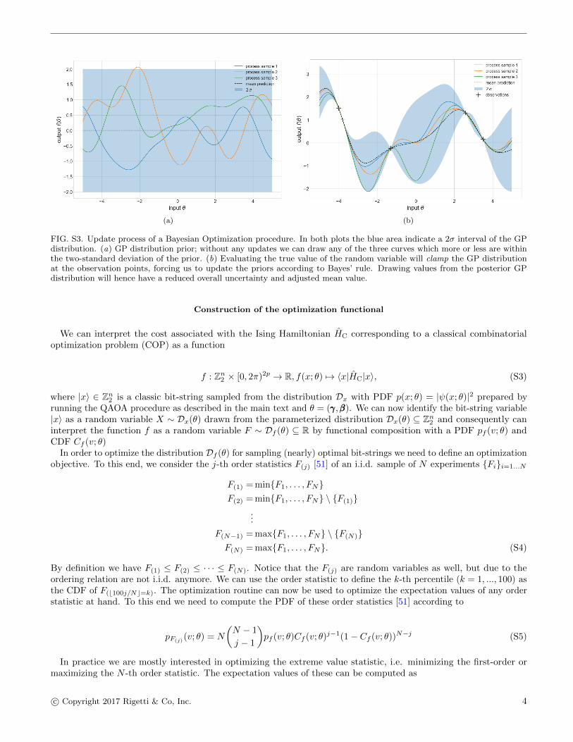
FIG. S3. Update process of a Bayesian Optimization procedure. In both plots the blue area indicate a 2σ interval of the GPdistribution. (a) GP distribution prior; without any updates we can draw any of the three curves which more or less are withinthe two-standard deviation of the prior. (b) Evaluating the true value of the random variable will clamp the GP distributionat the observation points, forcing us to update the priors according to Bayes’ rule. Drawing values from the posterior GPdistribution will hence have a reduced overall uncertainty and adjusted mean value.

Construction of the optimization functional

We can interpret the cost associated with the Ising Hamiltonian HC corresponding to a classical combinatorialoptimization problem (COP) as a function

f : Zn2 × [0, 2π)2p → R, f(x; θ) 7→ 〈x|HC|x〉, (S3)

where |x〉 ∈ Zn2 is a classic bit-string sampled from the distribution Dx with PDF p(x; θ) = |ψ(x; θ)|2 prepared byrunning the QAOA procedure as described in the main text and θ = (γγγ,βββ). We can now identify the bit-string variable|x〉 as a random variable X ∼ Dx(θ) drawn from the parameterized distribution Dx(θ) ⊆ Zn2 and consequently caninterpret the function f as a random variable F ∼ Df (θ) ⊆ R by functional composition with a PDF pf (v; θ) andCDF Cf (v; θ)

In order to optimize the distribution Df (θ) for sampling (nearly) optimal bit-strings we need to define an optimizationobjective. To this end, we consider the j-th order statistics F(j) [51] of an i.i.d. sample of N experiments {Fi}i=1...N

F(1) = min{F1, . . . , FN}F(2) = min{F1, . . . , FN} \ {F(1)}

...

F(N−1) = max{F1, . . . , FN} \ {F(N)}F(N) = max{F1, . . . , FN}. (S4)

By definition we have F(1) ≤ F(2) ≤ · · · ≤ F(N). Notice that the F(j) are random variables as well, but due to theordering relation are not i.i.d. anymore. We can use the order statistic to define the k-th percentile (k = 1, ..., 100) asthe CDF of F(b100j/Nc=k). The optimization routine can now be used to optimize the expectation values of any orderstatistic at hand. To this end we need to compute the PDF of these order statistics [51] according to

pF(j)(v; θ) = N

(N − 1

j − 1

)pf (v; θ)Cf (v; θ)j−1(1− Cf (v; θ))N−j (S5)

In practice we are mostly interested in optimizing the extreme value statistic, i.e. minimizing the first-order ormaximizing the N -th order statistic. The expectation values of these can be computed as

c© Copyright 2017 Rigetti & Co, Inc. 4

s1(θ) := 〈F(1)(θ)〉 = N

∫dv vpf (v; θ)(1− Cf (v; θ))N−1 (S6)

and

sN (θ) := 〈F(N)(θ)〉 = N

∫dv vpf (v; θ)Cf (v; θ)N−1 (S7)

Note that this approach also enables us to estimate the uncertainty of these random variables, giving qualityestimates of the sample. Despite looking horribly complicated, those values can readily be computed numericallyfrom a set of samples of the distribution Df (θ). A pseudo-code representation of the statistics calculation is given inalgorithm 2.

Gaussian Process description of the extreme value optimization

The extreme value functions sj(θ) : [0, 2π)2p → R, j = 1, N are generally not analytically known and typicallyexpensive to evaluate. Hence we have access to s(θ) only through evaluating it on a set of m points θ1:m [52] withcorresponding variables vi = s(θi) and noisy observations y1:m. Note that we drop the subscript j to denote thedistinction between minimal and maximal value functions as the approach is identical for either of them. To makeuse of Bayesian optimization techniques [32, 53] we assume that the variables v = v1:m are jointly Gaussian and thatthe observations y1:m are normally distributed given v, completing the construction of a Gaussian process (GP)[18].The distinction between the variable vi and its observation yi is important given that the expectation values S6and S7 are subject to sampling noise, due to finite samples, but also due to finite gate and readout fidelities and otherexperimental realities, and hence cannot be known exactly. We describe the GP using the moments of a multivariatenormal distribution

m(θ) =E[v(θ)] (S8)

k(θ, θ′) =E[(v(θ)− µ(θ))(v(θ′)− µ(θ′))] (S9)

and introduce the notation

v(θ) ∼ GP(m(θ), k(θ, θ′)) (S10)

This result summarizes the basic assumption that the extreme value statistic of the cost of best sampled bit-stringfollows a Gaussian distribution as a function of the parameters θ. While this might not be true, it proves to be a goodchoice for the unbiased prior in practice. To use the GP we need to specify the kernel function k(θ, θ′), which specifiesa measure of correlation between two observation points θ and θ′. Following [53] we use the Matern-2.5 kernel in thefollowing, but there are many alternative choices [18, 32].

The basic idea of Bayesian Optimization is to draw new observations y∗ at points θ∗ of the GP random variable vand iteratively use Bayes’ rule to condition the prior of v on y∗. This conditioning is particularly simple for GPs as itcan be performed analytically using the properties of multivariate normal distributions.

Algorithm 2: Statistics Calculation of Bit-String Distribution

Data: QAOA angle parameters θResult: value of a statistic s(θ) sampled from Df (θ)

CostValues ← empty List;for i← 1 to N do

bitString ← Sample(Dx(θ));cost ← Cost(bitString);CostValues.append(cost);

end// calculate the statistic of interest

s(θ) ← Statistic(CostValues);return s(θ);

c© Copyright 2017 Rigetti & Co, Inc. 5

To account for imperfect/noisy evaluations of the true underlying function we simply need to adjust the updaterule for the GP mean and kernels. This can also be done analytically and hence be directly applied to our case ofnumerically sampled extreme values statistics. For exhaustive details of the update rules, kernels and general GPproperties see Ref. [18]. It should be noted that the updated rules of Gaussian kernels require a matrix inversionwhich scales as O(m3) and hence can become prohibitively expensive when the number m of samples becomes large.Improving this scaling is an active area of research and early promising results such as Deep Networks for GlobalOptimization (DNGO) [33] provide surrogate methods for Gaussian processes with linear scaling.

So far we have only been concerned with updating the GP to reflect the incorporation of new knowledge. To closethe optimization loop we need a procedure to select the next sampling point θ∗. Choosing a point at random willessentially induce a random walk over the optimization parameter domain and might not be very efficient [46] (thoughthis is still better than a grid search). A nice improvement over this random walk is offered by Bayesian frameworkitself: due to the constantly updating the posterior distribution we can estimate the areas of highest uncertainty andconsequently chose the next point accordingly. However, this might bring the optimizer far away from the optimalpoint by trying to minimize the global uncertainty. To prevent the optimizer from drifting off we need a way tobalance its tendency to explore areas of high uncertainty with exploiting the search around the currently best knownvalue. This procedure is encapsulated in the acquisition function α(θ;Dm) where Dm = {(θi, yi)}i=1,...,m is the set ofobservations up to iteration m [32]. Since the posterior is Gaussian for every point θ there are many analytic ways toconstruct an acquisition function. Here, we use the Upper Confidence Bound (UCB) metric, which can be calculated as

αUCB(θ;Dm) = µm(θ) + βmσm(θ) (S11)

where βm is a hyperparameter controlling the explore-exploit behavior of the optimizer and µm(θ), σm(θ) are themean and variance of the Gaussian of the posterior GP restricted to point θ. Maximizing the acquisition function ofall values θ at each iteration step yields the next point for sampling from the unknown function s. For more details seeRef. [32]. A pseudo-code representation of the Bayesian Optimization routine is given in algorithm 3.

Comparison to Random Sampling

To demonstrate the applicability of the results beyond a single problem instance we ran the simulations on 5randomly chosen problem instances over a fourteen hour window on 19Q architecture. We recorded the optimizationtraces (cf. Fig. S4a) and calculated the empirical CDF (eCDF) for the time-to-optimum, i.e. the number of stepsbefore the optimizer reached the optimal value, as seen in Figs. 5, S4b. Note that we can estimate the optimal valueeasily for the problem at hand. We compared the empirical CDF (eCDF) to the CDF of a random sampling procedurethat follows a Bernoulli distribution B(N, p) with a success probability p = 2/219 and N = NstepsNshots samples. Theadditional factor 2 in the success probability is due to the inversion symmetry of the solution, i.e. there are twoequivalent solutions which minimize the cost and are related to each other by simply inverting each bit-assignment.The CDF for the Bernoulli random variable can then be easily written as:

Algorithm 3: Bayesian Optimization of QAOA Extreme Value Statistics

Data: statistics function fs and parameter range RθResult: optimal statistic fs(θopt)

GP Dist ← InitPrior;bestVal ← void;for i← 1 to N iter do

nextTheta ← SampleNextPoint(GP Dist);// calc. statistic with alg. 2

curVal ← Statistic(nextTheta);if curVal > bestVal then

bestVal ← curValendGP Dist ← Update(GP Dist, curVal, nextTheta)

endreturn bestVal;

c© Copyright 2017 Rigetti & Co, Inc. 6

(a) (b)

FIG. S4. (a) Traces for the normalized Maxcut cost for 83 independent runs of the algorithm on the 19Q chip for a fixedrandom problem instances of Fig. 3. Notice that most traces reach the optimal cost well before the cutoff at 55 steps. (b) Theperformance of our implementation of the clustering algorithm (red) can be compared to the performance of an algorithm thatsimply draws cluster assignments at random (green). It is clear that our algorithm generates the optimal assignment muchmore quickly than it would be expected by chance: the 95% confidence region for our empirical observations have very smalloverlap for the distribution given by random assignments, and the Kolmogorov-Smirnov statistic indicates we can reject the nullhypothesis of random assignments at a level higher than 99.9%.

TABLE S1. Kolmogorov-Smirnov statistics and significance values for the CDF shown in Fig. 5. All values are calculated withrespect to the exact random sampling CDF

eCDF KS α

empirical random bitstring sampling (Fig. 5) 0.077 1.559

Rigetti-QVM (Fig. 5) 0.838 1.273 · 10−7

19Q single instance (Fig. 5) 0.339 1.339 · 10−2

19Q randomized instances (Fig. S4b) 0.392 8.4451 · 10−4

P (success after k steps) = 1− (1− p)k∗Nshots (S12)

To compare the eCDF (red curve in Fig. S4b) to the random sampling CDF (green curve) we calculate theKolmogorov-Smirnov statistic between two eCDFs

KSn,m = supx|F1,n(x)− F2,m(x)| (S13)

where F1,n is the first eCDF with n points and F2,m is the second one with m points. Given the eCDFs of Fig. S4bwe find KS23,55 ≈ 0.392. We can calculate the significance level α by inverting the prescription for rejection of theNull-Hypothesis H0, i.e. the two eCDFs result from the same underlying distribution function:

KSn,m ≥ c(α)

√n+m

nm(S14)

where c(α) =√−0.5 log(α/2). Plugging in the empirical KS statistic we find that H0 can be rejected with a probability

p = 1 − α with α = 8.451 · 10−4. We also calculated the KS statistic for the curves in the main body of the textsummarized in Table. S1

c© Copyright 2017 Rigetti & Co, Inc. 7

5 6

15 17

0 1 2 4

10 11 12 13 14

5 6 7 8 9

15 16 17 18 19

0 1 2 4

10 11 12 13 14

5 6 7 8 9

15 16 17 18 19

0 1 2 4

10 11 12 13 14

5 6 7 8 9

15 16 17 18 19

0.18

0.59 0.

56

0.40 0.

570.71 0.

72

0.43

0.29

0.230.64

0.600.36

0.52

0.490.44

0.63

0.410.50

0.400.81

a

b

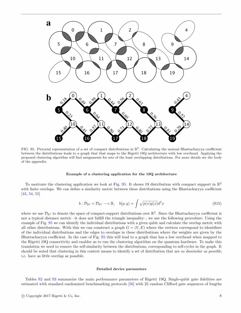
FIG. S5. Pictorial representation of a set of compact distributions in R2. Calculating the mutual Bhattacharyya coefficientbetween the distributions leads to a graph that that maps to the Rigetti 19Q architecture with low overhead. Applying theproposed clustering algorithm will find assignments for sets of the least overlapping distributions. For more details see the bodyof the appendix.

Example of a clustering application for the 19Q architecture

To motivate the clustering application we look at Fig. S5. It shows 19 distribution with compact support in R2

with finite overlaps. We can define a similarity metric between these distributions using the Bhattacharyya coefficient[43, 54, 55]

b : DR2 ×DR2 −→ R, b(p, q) =

∫ √p(x)q(x)d2x (S15)

where we use DR2 to denote the space of compact-support distributions over R2. Since the Bhattacharyya coefficient isnot a typical distance metric –it does not fulfill the triangle inequality–, we use the following procedure: Using theexample of Fig. S5 we can identify the individual distributions with a given qubit and calculate the overlap metric withall other distributions. With this we can construct a graph G = (V,E) where the vertices correspond to identifiersof the individual distributions and the edges to overlaps in these distributions where the weights are given by theBhattacharyya coefficient. In the case of Fig. S5 this will lead to a graph that has a low overhead when mapped tothe Rigetti 19Q connectivity and enables us to run the clustering algorithm on the quantum hardware. To make thistranslation we need to remove the self-similarity between the distributions, corresponding to self-cycles in the graph. Itshould be noted that clustering in this context means to identify a set of distribution that are as dissimilar as possible,i.e. have as little overlap as possible.

Detailed device parameters

Tables S2 and S3 summarize the main performance parameters of Rigetti 19Q. Single-qubit gate fidelities areestimated with standard randomized benchmarking protocols [56] with 25 random Clifford gate sequences of lengths

c© Copyright 2017 Rigetti & Co, Inc. 8

TABLE S2. Rigetti 19Q performance parameters — All of the parameters listed in this table have been measured atbase temperature T ≈ 10 mK. The reported T1’s and T ∗

2 ’s are averaged values over 10 measurements acquired at ωmax01 . The

errors indicate the standard deviation of the averaged value. Note that these estimates fluctuate in time due to multiple factors.

ωmaxr /2π ωmax

01 /2π η/2π T1 T ∗2 F1q FRO

MHz MHz MHz µs µs

0 5592 4386 -208 15.2± 2.5 7.2± 0.7 0.9815 0.938

1 5703 4292 -210 17.6± 1.7 7.7± 1.4 0.9907 0.958

2 5599 4221 -142 18.2± 1.1 10.8± 0.6 0.9813 0.970

3 5708 3829 -224 31.0± 2.6 16.8± 0.8 0.9908 0.886

4 5633 4372 -220 23.0± 0.5 5.2± 0.2 0.9887 0.953

5 5178 3690 -224 22.2± 2.1 11.1± 1.0 0.9645 0.965

6 5356 3809 -208 26.8± 2.5 26.8± 2.5 0.9905 0.840

7 5164 3531 -216 29.4± 3.8 13.0± 1.2 0.9916 0.925

8 5367 3707 -208 24.5± 2.8 13.8± 0.4 0.9869 0.947

9 5201 3690 -214 20.8± 6.2 11.1± 0.7 0.9934 0.927

10 5801 4595 -194 17.1± 1.2 10.6± 0.5 0.9916 0.942

11 5511 4275 -204 16.9± 2.0 4.9± 1.0 0.9901 0.900

12 5825 4600 -194 8.2± 0.9 10.9± 1.4 0.9902 0.942

13 5523 4434 -196 18.7± 2.0 12.7± 0.4 0.9933 0.921

14 5848 4552 -204 13.9± 2.2 9.4± 0.7 0.9916 0.947

15 5093 3733 -230 20.8± 3.1 7.3± 0.4 0.9852 0.970

16 5298 3854 -218 16.7± 1.2 7.5± 0.5 0.9906 0.948

17 5097 3574 -226 24.0± 4.2 8.4± 0.4 0.9895 0.921

18 5301 3877 -216 16.9± 2.9 12.9± 1.3 0.9496 0.930

19 5108 3574 -228 24.7± 2.8 9.8± 0.8 0.9942 0.930

l ∈ {2, 4, 8, 16, 32, 64, 128}. Readout fidelity is given by the assignment fidelity FRO = [p(0|0) + p(1|1)]/2, where p(b|a)is the probability of measuring the qubit in state b when prepared in state a. Two-qubit gate fidelities are estimatedwith quantum process tomography [45] with preparation and measurement rotations {I, Rx(π/2), Ry(π/2), Rx(π)}.The reported process fidelity F2q indicates the average fidelity between the ideal process and the measured processimposing complete positivity and trace preservation constraints. We further averaged over the extracted F2q from fourseparate tomography experiments. Qubit-qubit coupling strengths are extracted from Ramsey experiments with andwithout π-pulses on neighboring qubits.

c© Copyright 2017 Rigetti & Co, Inc. 9

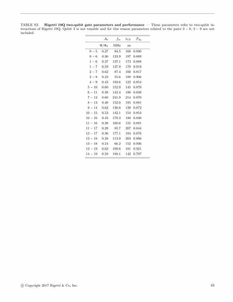
TABLE S3. Rigetti 19Q two-qubit gate parameters and performance — These parameters refer to two-qubit in-teractions of Rigetti 19Q. Qubit 3 is not tunable and for this reason parameters related to the pairs 3 − 8, 3 − 9 are notincluded.

A0 fm tCZ F2q

Φ/Φ0 MHz ns

0− 5 0.27 94.5 168 0.936

0− 6 0.36 123.9 197 0.889

1− 6 0.37 137.1 173 0.888

1− 7 0.59 137.9 179 0.919

2− 7 0.62 87.4 160 0.817

2− 8 0.23 55.6 189 0.906

4− 9 0.43 183.6 122 0.854

5− 10 0.60 152.9 145 0.870

6− 11 0.38 142.4 180 0.838

7− 12 0.60 241.9 214 0.870

8− 13 0.40 152.0 185 0.881

9− 14 0.62 130.8 139 0.872

10− 15 0.53 142.1 154 0.854

10− 16 0.43 170.3 180 0.838

11− 16 0.38 160.6 155 0.891

11− 17 0.29 85.7 207 0.844

12− 17 0.36 177.1 184 0.876

12− 18 0.28 113.9 203 0.886

13− 18 0.24 66.2 152 0.936

13− 19 0.62 109.6 181 0.921

14− 19 0.59 188.1 142 0.797

c© Copyright 2017 Rigetti & Co, Inc. 10