unsupervised joint part-of-speech tagging ...burcucan/necvabolucu...unsupervised joint...

UNSUPERVISED JOINT PART-OF-SPEECH TAGGING ANDSTEMMING FOR AGGLUTINATIVE LANGUAGES

SONDAN EKLEMELI DILLERDE GOZETIMSIZESZAMANLI SOZCUK TURU ISARETLEME VE

GOVDELEME

Necva BOLUCU

Asst. Prof. Dr. Burcu CAN BUGLALILAR

Supervisor

Submitted to Graduate School of Science and Engineering of

Hacettepe University

as a Partial Fulfillment to the Requirements

for the Award of the Degree of Master of Science

in Computer Engineering

2017

ABSTRACT

Unsupervised Joint Part-of-Speech Tagging and Stemming ForAgglutinative Languages

Necva BOLUCU

Master of Science,Computer Engineering DepartmentSupervisor: Asst. Prof. Dr. Burcu CAN BUGLALILAR

June 2017, 108 pages

Part of Speech (PoS) tagging is the task of assigning each word an appropriate part of speech

tag in a given sentence regarding its syntactic role such as verb, noun, adjective etc. Various

approaches have already been proposed for this task. However, the number of word forms

in morphologically rich and productive agglutinative languages is theoretically infinite. This

variety in word forms causes sparsity problem in the tagging task for agglutinative languages.

In this thesis, we aim to deal with this problem in agglutinative languages by performing PoS

tagging and stemming simultaneously. Stemming is the process of finding the stem of a word

by removing its suffixes. Joint PoS tagging and stemming reduces sparsity by using stems

and suffixes instead of words. Furthermore, we incorporate semantic features to capture

similarity between stems and their derived forms by using neural word embeddings.

In this thesis, we present a fully unsupervised Bayesian model using Hidden Markov Model

(HMM) for joint PoS tagging and stemming for agglutinative languages. The results indi-

cate that using stems and suffixes rather than full words outperforms a simple word-based

Bayesian HMM model for especially agglutinative languages. Combining semantic features

yields a significant improvement in stemming.

i

http://cs.hacettepe.edu.tr

Anahtar Kelimeler: unsupervised learning, part-of-speech (PoS) tagging, stemming,

Bayesian learning, Hidden Markov model (HMM), semantic, neural word embeddings

ii

OZET

Sondan Eklemeli Dillerde Gozetimsiz Eszamanlı Sozcuk Turu Isaretlemeve Govdeleme

Necva BOLUCU

Yuksek Lisans,Bilgisayar MuhendisligiDanısman: Yrd. Doc. Dr. Burcu CAN BUGLALILAR

Haziran 2017, 108 sayfa

Sozcuk turu isaretleme, cumledeki fiil, isim, sıfat v.b. sozdizimsel rolune bakarak her bir

sozcuge uygun etiketin atanmasıdır. Bu islem icin cesitli yontemler onerilmistir. Mor-

folojik olarak zengin ve uretken sondan eklemeli dillerde sozcuk formlarının sayısı teorik

olarak sonsuzdur. Sozcuk formlarındaki bu cesitlilik, sondan eklemeli dillerde etiketleme

isleminde seyreklik problemi yaratmaktadır. Bu tezde sozcuk turu isaretleme ve govdeleme

islemlerini eszamanlı gerceklestirerek sondan eklemeli dillerde bu problemin ustesinden

gelmeyi amaclamaktayız. Govdeleme, bir sozcugu eklerinden ayırarak govdeyi bulma islemidir.

Birlesik sozcuk turu isaretleme ve govdeleme, sozcukler yerine govde ve ekler kullanarak

seyreklik problemini azaltmaktadır. Ayrıca, govde ve govdeden turetilmis sozcuk arasındaki

benzerligi yakalamak icin anlamsal ozelliklerden yararlanmaktayız.

Bu tezde, sondan eklemeli dillerde birlesik sozcuk turu isaretleme ve govdeleme islemi

gerceklestirmek icin tamamen gozetimsiz Bayesian Saklı Markov modeli sunulmustur. Sonuclar,

ozellikle sondan eklemeli diller icin sozcukler yerine govdeler ve eklerinin kullanılmasının

sozcuk tabanlı Bayesian HMM modelinden daha iyi oldugunu gostermektedir. Anlamsal

ozelliklerin eklenmesi ise govdelemede belirgin bir iyilesme gostermektedir.

iii

Keywords: gozetimsiz ogrenme,sozcuk turu isaretleyici, govdeleme, Bayesian ogrenme,

saklı Markov model

iv

ACKNOWLEDGEMENTS

First and foremost, I would like to wholeheartedly thank to my excellent supervisor Asst.

Prof. Dr. Burcu Can Buglalılar for her endless patience, valuable advice, encouragements

and immeasurable amount of guidance in this thesis. At every stage of this thesis, she sup-

ported me with her knowledge. I can say for sure that I have always felt fortunate to work

under her inspiring supervision.

Besides I would like to thank my thesis committee members for insightful comments for this

thesis.

In addition, I would like to thank everbody who supported and contributed to this study.

Especially, I would like to thank my office mate Selma Dilek; she was not only an office mate

but also a sincere friend. I am also obliged to my reading group friends for their friendship

and support.

Finally, I thank my beloved family for their continual support throughout my educational

life. They have always believed in me and encouraged me with their best wishes.

This work is supported by the Scientific and Technological Research Council of Turkey

(TUBITAK) with the project number EEEAG-115E464.

v

CONTENTS

Page

ABSTRACT . . . . . . . . . . . . . . . . . . . . . . . . . . . . . . . . . . . . . . . . . . . . . . . . . . . . . . . . . . . . . . . . . . . . . . . . . . . . . . . . . . i

OZET . . . . . . . . . . . . . . . . . . . . . . . . . . . . . . . . . . . . . . . . . . . . . . . . . . . . . . . . . . . . . . . . . . . . . . . . . . . . . . . . . . . . . . . . . iii

ACKNOWLEDGMENTS . . . . . . . . . . . . . . . . . . . . . . . . . . . . . . . . . . . . . . . . . . . . . . . . . . . . . . . . . . . . . . . . . . . v

CONTENTS . . . . . . . . . . . . . . . . . . . . . . . . . . . . . . . . . . . . . . . . . . . . . . . . . . . . . . . . . . . . . . . . . . . . . . . . . . . . . . . . . . vi

FIGURES . . . . . . . . . . . . . . . . . . . . . . . . . . . . . . . . . . . . . . . . . . . . . . . . . . . . . . . . . . . . . . . . . . . . . . . . . . . . . . . . . . . . . viii

TABLES . . . . . . . . . . . . . . . . . . . . . . . . . . . . . . . . . . . . . . . . . . . . . . . . . . . . . . . . . . . . . . . . . . . . . . . . . . . . . . . . . . . . . . x

ABBREVIATIONS. . . . . . . . . . . . . . . . . . . . . . . . . . . . . . . . . . . . . . . . . . . . . . . . . . . . . . . . . . . . . . . . . . . . . . . . . . xi

1. INTRODUCTION. . . . . . . . . . . . . . . . . . . . . . . . . . . . . . . . . . . . . . . . . . . . . . . . . . . . . . . . . . . . . . . . . . . . . . . . 1

1.1. Overview . . . . . . . . . . . . . . . . . . . . . . . . . . . . . . . . . . . . . . . . . . . . . . . . . . . . . . . . . . . . . . . . . . . . . . . . . . . . . . . 1

1.2. Motivation . . . . . . . . . . . . . . . . . . . . . . . . . . . . . . . . . . . . . . . . . . . . . . . . . . . . . . . . . . . . . . . . . . . . . . . . . . . . . . 2

1.3. Research Questions . . . . . . . . . . . . . . . . . . . . . . . . . . . . . . . . . . . . . . . . . . . . . . . . . . . . . . . . . . . . . . . . . . . . 3

2. BACKGROUND . . . . . . . . . . . . . . . . . . . . . . . . . . . . . . . . . . . . . . . . . . . . . . . . . . . . . . . . . . . . . . . . . . . . . . . . . 5

2.1. Linguistic Background . . . . . . . . . . . . . . . . . . . . . . . . . . . . . . . . . . . . . . . . . . . . . . . . . . . . . . . . . . . . . . . . . 5

2.2. Machine Learning Background. . . . . . . . . . . . . . . . . . . . . . . . . . . . . . . . . . . . . . . . . . . . . . . . . . . . . . . . 9

2.3. Inference . . . . . . . . . . . . . . . . . . . . . . . . . . . . . . . . . . . . . . . . . . . . . . . . . . . . . . . . . . . . . . . . . . . . . . . . . . . . . . . . 13

2.4. Conclusion. . . . . . . . . . . . . . . . . . . . . . . . . . . . . . . . . . . . . . . . . . . . . . . . . . . . . . . . . . . . . . . . . . . . . . . . . . . . . . 14

3. RELATED WORK . . . . . . . . . . . . . . . . . . . . . . . . . . . . . . . . . . . . . . . . . . . . . . . . . . . . . . . . . . . . . . . . . . . . . . . 15

3.1. Introduction . . . . . . . . . . . . . . . . . . . . . . . . . . . . . . . . . . . . . . . . . . . . . . . . . . . . . . . . . . . . . . . . . . . . . . . . . . . . 15

3.2. Literature Review on Unsupervised Part of Speech Tagging . . . . . . . . . . . . . . . . . . . . . . . . 15

3.3. Literature Review of Cooperative Learning of Part of Speech Tagging . . . . . . . . . . . . . 21

3.4. Literature Review on Stemming . . . . . . . . . . . . . . . . . . . . . . . . . . . . . . . . . . . . . . . . . . . . . . . . . . . . . . . 22

3.5. Conclusion. . . . . . . . . . . . . . . . . . . . . . . . . . . . . . . . . . . . . . . . . . . . . . . . . . . . . . . . . . . . . . . . . . . . . . . . . . . . . . 28

4. MODEL. . . . . . . . . . . . . . . . . . . . . . . . . . . . . . . . . . . . . . . . . . . . . . . . . . . . . . . . . . . . . . . . . . . . . . . . . . . . . . . . . . . 29

4.1. Introduction . . . . . . . . . . . . . . . . . . . . . . . . . . . . . . . . . . . . . . . . . . . . . . . . . . . . . . . . . . . . . . . . . . . . . . . . . . . . 29

4.2. Baseline Bayesian HMM Model . . . . . . . . . . . . . . . . . . . . . . . . . . . . . . . . . . . . . . . . . . . . . . . . . . . . . . 29

4.3. Joint Models for PoS Tagging and Stemming . . . . . . . . . . . . . . . . . . . . . . . . . . . . . . . . . . . . . . . . 31

vi

5. EXPERIMENTS AND RESULTS . . . . . . . . . . . . . . . . . . . . . . . . . . . . . . . . . . . . . . . . . . . . . . . . . . . . . . 42

5.1. Datasets . . . . . . . . . . . . . . . . . . . . . . . . . . . . . . . . . . . . . . . . . . . . . . . . . . . . . . . . . . . . . . . . . . . . . . . . . . . . . . . . . 42

5.2. Evaluation Metrics . . . . . . . . . . . . . . . . . . . . . . . . . . . . . . . . . . . . . . . . . . . . . . . . . . . . . . . . . . . . . . . . . . . . . 43

5.3. Experiments . . . . . . . . . . . . . . . . . . . . . . . . . . . . . . . . . . . . . . . . . . . . . . . . . . . . . . . . . . . . . . . . . . . . . . . . . . . . 46

5.4. Conclusion. . . . . . . . . . . . . . . . . . . . . . . . . . . . . . . . . . . . . . . . . . . . . . . . . . . . . . . . . . . . . . . . . . . . . . . . . . . . . . 63

6. CONCLUSION. . . . . . . . . . . . . . . . . . . . . . . . . . . . . . . . . . . . . . . . . . . . . . . . . . . . . . . . . . . . . . . . . . . . . . . . . . . 65

6.1. Conclusion. . . . . . . . . . . . . . . . . . . . . . . . . . . . . . . . . . . . . . . . . . . . . . . . . . . . . . . . . . . . . . . . . . . . . . . . . . . . . . 65

6.2. Future Research Directions . . . . . . . . . . . . . . . . . . . . . . . . . . . . . . . . . . . . . . . . . . . . . . . . . . . . . . . . . . . . 66

A APPENDIX : PoS TAGSET REDUCTION . . . . . . . . . . . . . . . . . . . . . . . . . . . . . . . . . . . . . . . . . . . . 67

B APPENDIX : Word2vec DATA. . . . . . . . . . . . . . . . . . . . . . . . . . . . . . . . . . . . . . . . . . . . . . . . . . . . . . . . . . 70

C APPENDIX : RESULTS FOR 12K DATASETS . . . . . . . . . . . . . . . . . . . . . . . . . . . . . . . . . . . . . . . 71

REFERENCES . . . . . . . . . . . . . . . . . . . . . . . . . . . . . . . . . . . . . . . . . . . . . . . . . . . . . . . . . . . . . . . . . . . . . . . . . . . . . . . 80

vii

FIGURES

Page

2.1. Structure of a typical word in an agglutinative language . . . . . . . . . . . . . . . . . . . . . . . . . 7

2.2. Stem of word gecmis according to different PoS . . . . . . . . . . . . . . . . . . . . . . . . . . . . . . . . . 7

2.3. A Bayesian network specifying conditional independence relations for a hid-

den Markov model. . . . . . . . . . . . . . . . . . . . . . . . . . . . . . . . . . . . . . . . . . . . . . . . . . . . . . . . . . . . . . . . . 9

2.4. An illustration of the CRP . . . . . . . . . . . . . . . . . . . . . . . . . . . . . . . . . . . . . . . . . . . . . . . . . . . . . . . . . 13

3.1. The binary tree obtained from Brown clustering . . . . . . . . . . . . . . . . . . . . . . . . . . . . . . . . . 16

3.2. Bigram HMM .. . . . . . . . . . . . . . . . . . . . . . . . . . . . . . . . . . . . . . . . . . . . . . . . . . . . . . . . . . . . . . . . . . . . . 17

3.3. Trigram HMM.. . . . . . . . . . . . . . . . . . . . . . . . . . . . . . . . . . . . . . . . . . . . . . . . . . . . . . . . . . . . . . . . . . . . . 17

3.4. Contextualised HMM Tagger . . . . . . . . . . . . . . . . . . . . . . . . . . . . . . . . . . . . . . . . . . . . . . . . . . . . . . 18

3.5. Infinite HMM Tagger . . . . . . . . . . . . . . . . . . . . . . . . . . . . . . . . . . . . . . . . . . . . . . . . . . . . . . . . . . . . . . 20

3.6. Joint PoS tagging and segmentation proposed by Sirts and Tanel [1] . . . . . . . . . . . 21

4.1. The plate diagram of the Bayesian HMM with symmetric Dirichlet priors. . . . . 30

4.2. The plate diagram of the stem based Bayesian HMM. . . . . . . . . . . . . . . . . . . . . . . . . . . . 32

4.3. The plate diagram of the stem and suffix-based Bayesian HMM. . . . . . . . . . . . . . . . 34

4.4. Dependency of suffixes in an example Turkish sentence. . . . . . . . . . . . . . . . . . . . . . . . . 37

4.5. The plate diagram of the affix transition-based Bayesian HMM. . . . . . . . . . . . . . . . . 38

4.6. Stem and Transition based Bayesian HMM. . . . . . . . . . . . . . . . . . . . . . . . . . . . . . . . . . . . . . . 40

5.1. Example sentence with its specific and corresponding universal POS tags. . . . . 43

5.2. Sensitivity of hyperparameter sets for PoS tagging performance in Turkish . . . . 47

5.3. Sensitivity of parameter set for stemming performance of Turkish . . . . . . . . . . . . . 50

5.4. Features summary of proposed model for Turkish . . . . . . . . . . . . . . . . . . . . . . . . . . . . . . . 50

5.5. Sensitivity of dataset for PoS performance of Hungarian . . . . . . . . . . . . . . . . . . . . . . . . 51

viii

TABLES

2.1. PoS tag list proposed by Petrol et al. [2] . . . . . . . . . . . . . . . . . . . . . . . . . . . . . . . . . . . . . . . . . . 8

5.1. Datasets used in the experiments . . . . . . . . . . . . . . . . . . . . . . . . . . . . . . . . . . . . . . . . . . . . . . . . . . 42

5.2. Turkish PoS tagging results for different hyperparameter sets . . . . . . . . . . . . . . . . . . . 48

5.3. Turkish stemming results for different hyperparameter sets . . . . . . . . . . . . . . . . . . . . . 49

5.4. Hungarian24k PoS tagging results for different hyperparameter sets . . . . . . . . . . . 52

5.5. Hungarian24k stemming results for different hyperparameter sets . . . . . . . . . . . . . . 54

5.6. Finnish24k PoS tagging results for different hyperparameter sets . . . . . . . . . . . . . . . 55

5.7. Finnish24k stemming results for different hyperparameter sets . . . . . . . . . . . . . . . . . 56

5.8. Basque24k PoS tagging results for different hyperparameter sets . . . . . . . . . . . . . . . 57

5.9. Basque24k stemming results for different hyperparameter sets . . . . . . . . . . . . . . . . . 58

5.13. Examples to correct and incorrect stems of Turkish . . . . . . . . . . . . . . . . . . . . . . . . . . . . . . 59

5.14. Examples to correct and incorrect stems of Hungarian . . . . . . . . . . . . . . . . . . . . . . . . . . 59

5.10. Penn 24K PoS tagging results for different hyperparameter sets . . . . . . . . . . . . . . . . 60

5.11. udEnglish 24K PoS tagging results for different hyperparameter sets . . . . . . . . . . 61

5.12. udEnglish 24K stemming results for different hyperparameter sets . . . . . . . . . . . . . 62

5.15. Examples to correct and incorrect stems of Finnish . . . . . . . . . . . . . . . . . . . . . . . . . . . . . . 63

5.16. Examples to correct and incorrect stems of Basque . . . . . . . . . . . . . . . . . . . . . . . . . . . . . . 63

5.17. Examples to correct and incorrect stems of English . . . . . . . . . . . . . . . . . . . . . . . . . . . . . . 63

1.1. The mapping of the Universal tagset to the Penn Treebank tagset. . . . . . . . . . . . . . . 67

1.2. The mapping of the Universal tagset to the FinnTreeBank tagset . . . . . . . . . . . . . . . 67

1.3. The mapping of the Universal tagset to UD Basque TreeBank tagset . . . . . . . . . . . 68

1.4. The mapping of the Universal tagset to UD Hungarian TreeBank tagset . . . . . . . 68

1.5. The mapping of the Universal tagset to UD English TreeBank tagset. . . . . . . . . . . 69

1.6. The mapping of the Universal tagset to the Metu-Sabancı Turkish Treebank

tagset . . . . . . . . . . . . . . . . . . . . . . . . . . . . . . . . . . . . . . . . . . . . . . . . . . . . . . . . . . . . . . . . . . . . . . . . . . . . . . . . 69

3.1. Hungarian12K PoS tagging results for different hyperparameter sets . . . . . . . . . . . 71

ix

3.2. Hungarian12k stemming results for different hyperparameter sets . . . . . . . . . . . . . . 72

3.3. Finnish 12K PoS tagging results for different hyperparameter sets . . . . . . . . . . . . . 73

3.4. Finnish 12K stemming results for different hyperparameter sets . . . . . . . . . . . . . . . . 74

3.5. Basque 12K PoS tagging results for different hyperparameter sets. . . . . . . . . . . . . . 75

3.6. Basque 12K stemming results for different hyperparameter sets . . . . . . . . . . . . . . . . 76

3.7. Penn 12K PoS tagging results for different hyperparameter sets . . . . . . . . . . . . . . . . 77

3.8. udEnglish 12K PoS tagging results for different hyperparameter sets . . . . . . . . . . 78

3.9. udEnglish 12K stemming results for different hyperparameter sets . . . . . . . . . . . . . 79

x

ABBREVIATIONS

CRF Conditional Random Fields

CRP Chinese Restaurant Process

CW Chinese Whispers

ddCRP distance independent CRP

DP Drichlet Process

EM Expectation Maximization

FSM Frakes and Fox Similarity Metric

GRAS GRaph-based Stemmer

HDP Hierarchical Drichlet Process

HMM Hidden Markov Model

HPS High Precision Stemmer

ICF Index Compression Factor

iHMM infinite HMM

IR Information Retrieval

KL Kullback-Leibler

LSA Latent Semantic Analysis

MAP Maximuml a Posteriori

MCMC Markov Chain Monte Carlo

MCRS Mean Number of Characters and Removed in forming Stems

MDL Minimum Description Length

MEM Maximum Entropy Model

MHD Mean and Median Modified Hamming Distance

ML Maximum Likelihood

xi

MLE Maximum Likelihood Estimation

MMI Maximum Mutual Information

MWC Mean Number of Words per Conflation Class

NLP Natural Language Processing

NMI Normalized Mutual Information

NWSF Number of Words and Stems diFfer

OOV out-of-Vcabulary

PMF Probability Mass Function

PoS Part of Speech

RF Relative Frequency

SVD Singular Value Decomposition

TTS Text to Speech

VI Variation of Information

WSJ Wall Street Journal

YASS Yet Another Suffix Striper

xii

1. INTRODUCTION

1.1. Overview

Parts of speech play a crucial role in defining the structure and meaning of a sentence in any

language. Words can be labeled with different parts of speech depending their syntactic roles

in the sentence. Assigning each word a part of speech such as noun, verb, adjective, etc. is

called Part of Speech (PoS) tagging task in Natural Language Processing (NLP). It is one

of the early tasks in NLP. PoS taggers take a sentence as input and generate a list of tuples

(word/tag) as output, where each word is assigned to related tag.

Example The sentence

Bunu zaten biliyordum. (I have already known that.) is tagged as:

Bunu/Pron zaten/Adv biliyordum/Verb ./Punc

This task determines the syntactic features of the words such as gender, tense, etc. [3].

Stemming is the process of removing inflectional affixes from a word. The aim of stem-

ming is to reduce the morphological variants to a linguistically correct stem from which all

different word forms are derived.

Example : kitaplar (books), kitapta (in the book), kitaplarım (my books) have the same stem

kitap (book)

PoS tagging and stemming have been playing significant roles in several NLP applications.

Thus, small improvements on these tasks have the potential to yield larger improvements in

many NLP tasks like Information Retrieval (IR), Linguistic Research, Text to Speech (TTS),

Information Extraction and Shallow Parsing.

One of the challenges of PoS tagging is ambiguity. Many words can take several parts of

speech. For example booking can be a noun (e.g. We made the booking three months ago.)

or a verb (e.g. She is booking a table for four at their favorite restaurant.). Such a problem

is common in many languages. The other challenge is out-of-vocabulary (OOV) problem.

There will be many words which have not been seen in training.

1

1.2. Motivation

Agglutinative languages like Turkish are morphologically rich and productive. Turkish has

nearly 23,000 stems and words formed by gluing suffixes to stems. Therefore, infinite num-

ber of words can be formed theoretically [4]. Due to rich morphology, these languages raises

several challenges in PoS tagging and stemming.

There is a strong mutual relation between stemming and PoS tagging. Modeling joint PoS

tagging and stemming helps to solve these challenges. Joint PoS tagging and stemming helps

tackle the OOV problem by reducing the lexicon size. For instance, the words kitaplarda (in

books), kitaplar (books), kitap (book), kitapta (in the book), kitaplarım (my books), kitaptan

(from the book), kitapları ((their) books), kitapla (with the book), kitaplara (to the books)

are inflected from the stem kitap (book). By mapping the different word forms to the same

stem, we can reduce the word forms to a single stem by also reducing the dictionary size and

increasing the frequency of occurrence of the words. Joint PoS tagging and stemming also

helps to determine how to split a word as a stem and a affix. For example, the words koyun

can be split as koy+un (put) or koyun+# (sheep) depending on its tag. PoS tag of the word

helps to choose the correct stem.

Pipeline approaches solve tasks in order, for example stemming after then PoS tagging. One

drawback of pipeline approaches is the error propagation where the errors accumulate in all

stages. Joint models can avoid this kind of problem and achieve a better performance on both

sub-tasks.

This is why a joint model would be more effective to handle PoS tagging and stemming

instead of a pipeline approach [5].

Although supervised PoS tagging and stemming models perform better than unsupervised

models, supervised models are applicable only to a set of well-studied languages that have

labeled corpora available. However, more than 99% of the languages in the world are still

considered less-studied and resource scarce [6]. Therefore, it indicates that developing un-

supervised models is crucially needed for these languages.

In this thesis, we extend the fully unsupervised Bayesian PoS tagging model [7] for aggluti-

native languages. Instead of using words, we enhance the model by using stems, affixes and

2

semantic features. We primarily focus on Turkish as an agglutinative language. However,

the models will be applicable to all languages.

1.3. Research Questions

These are the research questions that are aimed to be answered in this thesis:

• Can unsupervised PoS tagging be improved by integrating the stemming task jointly to

the same learning mechanism? Does joint model help to reduce the sparsity problem

in PoS tagging?

• Can we enhance stemming and PoS tagging results by integrating semantic features to

the joint model?

1.3.1. Thesis Structure

The structure of the thesis is as follows:

Chapter 2 details essential background knowledge to understand the thesis. It starts with

linguistic background, describes agglutinative languages and challenges of these languages.

Then, we explain machine learning methods that we used in this thesis.

Chapter 3 provides an overview of the previous studies on PoS tagging and stemming. We

focus on HMM for PoS tagging and unsupervised methods on stemming. We also discuss

evaluation algorithms for PoS tagging and stemming. This chapter also presents studies on

Turkish PoS tagging and stemming.

Chapter 4 describes a novel joint model in which PoS tagging and stemming are learned

cooperatively and simultaneously. First, we present the baseline model that constructed on.

Finally, the inference algorithm is described.

Chapter 5 reports our experimental results and compare PoS tagging and stemming results

with other approaches in the literature for agglutinative languages and morphologically poor

languages. We end this chapter with the analysis of parameters.

3

Finally, Chapter 6 concludes this thesis with a brief summary of our work with contributions

made to the fields of PoS tagging and stemming and proposes future topics to be studied

based on the the study in both fields.

4

2. BACKGROUND

In this chapter, we review background information to follow the approaches presented in this

thesis. We start by explaining the linguistic background in Section 2.1.. Then, we focus on

the machine learning background in Section 2.2..

2.1. Linguistic Background

“There are close on 7,000 languages in the world, and half of them have fewer than 7,000

Speakers each, less than a village. What is more, 80% of the world’s languages have fewer

than 100,000 speakers.”(Ostler 2008)

The spoken languages in the world can be classified as follows: Inflective languages, agglu-

tinative languages, isolating languages, and incorporating languages.

Inflective languages consist of stems with variable terminations or suffixes which were once

independent words like Latin. Agglutinative languages consist of more than one, and pos-

sibly many morphemes. Examples of agglutinative languages are Turkish and Hungarian.

Isolating language is a language in which meaning is created by supplemental words. Thus,

almost every word consists of a single morpheme in the language. Latin, Spanish, English,

Chinese, and Mandarin are examples of isolating languages. Incorporating languages are

referred as polysynthetic languages. A single - though extensively long - word may repre-

sent an entire phrase, or even a sentence, including a verb, an adjective and even an object

in incorporating. This language is often used to refer to Native American languages such as

Alabama, Dakota.

In this chapter, we provide a brief description of the morphological structure of Turkish as

an agglutinative language to ease the understanding of this thesis.

2.1.1. Morphology

Morphology is about the internal structure of words and operates with the subword units

called morphemes. It is also an interface between phonology and syntax, where morpholog-

ical forms as constituents carry both syntactic and phonetic information. For example, word

5

kitapcılar (booksellers) is composed from root kitap (book), and two bound morphemes -cı

and -lar.

Agglutinative languages are morphologically productive languages that contain a set of rules

for morphological composition that generate a considerable amount of word forms by the

concatenation of morphemes [8].

Morphemes can be either roots or affixes. Affixes can be either inflectional or derivational.

Roots can take derivational and inflectional affixes; therefore, a root can be seen in a large

number of different word forms. Various suffixes and their combinations make a complex

problem to find stems in agglutinative languages.

Example Some of the word forms that are built from the root basar(-mak) ((to) succeed) are

as follows:

basar(-mak) - ((to) succeed)

basarı - (success)

basarısız - (unsuccessful)

basarısızlas(-mak) - ((to) become unsuccessful)

basarısızlastır(-mak) - ((to) make one unsuccessful)

basarısızlastırıcı - (maker of unsuccessful ones)

basarısızlastırıcılas(-mak) - ((to) become a maker of unsuccessful ones)

basarısızlastırıcılastır(-mak) - ((to) make one a maker of unsuccessful ones)

Inflectional suffixes add appropriate syntactic features such as gender, tense, etc. [3] to the

word whereas derivational suffixes change the meaning of the word. For instance, the suffix

-ler in the word kalemler (pencils) is inflectional because it marks the plurality of the word

kalem (pencil) and kalem (pencil) and kalemler (pencils) share the same meaning. The suffix

-gi in the word silgi (eraser) is derivational because it changes the meaning of the word from

an action to a tool. Here, the derivational suffix also changes the PoS tag of the word.

A stem is the base of an inflected word. The stem of a word does not necessarily have to be

indivisible and can consist of a root that has derivational suffixes attached to it.

6

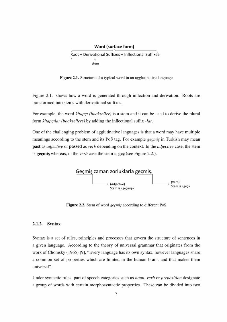
Root + Derivational Suffixes + Inflectional Suffixes

Word (surface form)

stem

Figure 2.1. Structure of a typical word in an agglutinative language

Figure 2.1. shows how a word is generated through inflection and derivation. Roots are

transformed into stems with derivational suffixes.

For example, the word kitapcı (bookseller) is a stem and it can be used to derive the plural

form kitapcılar (booksellers) by adding the inflectional suffix -lar.

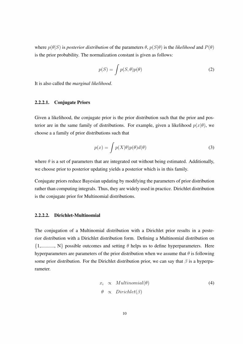
One of the challenging problem of agglutinative languages is that a word may have multiple

meanings according to the stem and its PoS tag. For example gecmis in Turkish may mean

past as adjective or passed as verb depending on the context. In the adjective case, the stem

is gecmis whereas, in the verb case the stem is gec (see Figure 2.2.).

Geçmiş zaman zorluklarla geçmiş.

(Adjective)Stem is «geçmiş»

(Verb)Stem is «geç»

Figure 2.2. Stem of word gecmis according to different PoS

2.1.2. Syntax

Syntax is a set of rules, principles and processes that govern the structure of sentences in

a given language. According to the theory of universal grammar that originates from the

work of Chomsky (1965) [9], “Every language has its own syntax, however languages share

a common set of properties which are limited in the human brain, and that makes them

universal”.

Under syntactic rules, part of speech categories such as noun, verb or preposition designate

a group of words with certain morphosyntactic properties. These can be divided into two

7

Table 2.1. PoS tag list proposed by Petrol et al. [2]

Tag Definition ExampleVERB Verbs (all tenses and modes) gitmis, gelecek, yuzuyorNOUN Nouns (Common and proper) kitap, Ahmet, gozlukPRON Pronouns Ben, onlarADJ Adjectives sıcak, genc, kucukADV Adverbs iceri, hızlıcaADP Adpositions (prepositions and postpositions gibi, degil, uzereCONJ Conjunctions fakat, oysaki, ustelikDET Determiners bir , buNUM Cardinal numbers onbes ,ikiPRT particles or other function words gore, kadarX Other (foreign words, types, abbreviations) TDK, THY. Punctiation ?, !, :

categories: closed class types and open class types. Closed classes have fixed number of

members, whereas open classes may accept many members, thereby they can infinite number

of members.

There are four main open classes; noun, verb, adjective, adverb.

Noun class includes the words that mostly correspond to people, places, or other things.

The verb class includes the words referring to actions e.g. git(mek) ((to) go), bil(mek) ((to)

know), konus(mak) ((to) talk).

The adverb class describes and gives information about a verb, adjective, adverb or phrase.

For instance, in sentence “Hızlı konusurum.” (“I speak fast”), the adverb hızlı modifies the

verb konusurum.

The adjective class modifies nouns and pronouns by describing a particular quality of the

word. For example, in noun phrase calıskan ogrenci (hardworking student), calıskan modi-

fies student.

Closed classes differ from language to language differently from open classes. Major closed

classes are prepositions, determiners, pronouns, conjunctions, participles, numerals.

Petrov et al. (2011) [2] propose a Universal PoS tag set that defines 12 universal categories.

8

2.2. Machine Learning Background

2.2.1. Hidden Markov Models

A Hidden Markov Model (HMM) is a method for representing probability distributions over

sequences of observations. A sequence of hidden states (S1, S2, ....) is generated according

to a Markov process. Conditioned on the hidden states, we observe (Y1, Y2, ....) where it is

assumed that the Yi is conditionally independent of everything else given the Si and the Si+1

is conditionally independent of everything else given the Si.

S1

YTY2Y1

S2 S3

Y3

ST

Figure 2.3. A Bayesian network specifying conditional independence relations for a hiddenMarkov model.

2.2.2. Bayesian Modeling

Bayesian modeling defines the probability of an instance with respect to value of parame-

ters, latent variables or hypotheses. A Bayesian model can be parametric or non-parametric.

The Bayesian parametric models have predefined number of parameters. The Bayesian non-

parametric models have countably infinite parameters that grows with data. Bayesian mod-

eling derives from Bayes’ theorem:

p(θ|S) =p(S|θ)p(θ)p(S)

(1)

9

where p(θ|S) is posterior distribution of the parameters θ, p(S|θ) is the likelihood and P (θ)

is the prior probability. The normalization constant is given as follows:

p(S) =

∫p(S, θ)p(θ) (2)

It is also called the marginal likelihood.

2.2.2.1. Conjugate Priors

Given a likelihood, the conjugate prior is the prior distribution such that the prior and pos-

terior are in the same family of distributions. For example, given a likelihood p(x|θ), we

choose a a family of prior distributions such that

p(x) =

∫p(X|θ)p(θ)d(θ) (3)

where θ is a set of parameters that are integrated out without being estimated. Additionally,

we choose prior to posterior updating yields a posterior which is in this family.

Conjugate priors reduce Bayesian updating by modifying the parameters of prior distribution

rather than computing integrals. Thus, they are widely used in practice. Dirichlet distribution

is the conjugate prior for Multinomial distributions.

2.2.2.2. Dirichlet-Multinomial

The conjugation of a Multinomial distribution with a Dirichlet prior results in a poste-

rior distribution with a Dirichlet distribution form. Defining a Multinomial distribution on

{1,..........., N} possible outcomes and setting θ helps us to define hyperparameters. Here

hyperparameters are parameters of the prior distribution when we assume that θ is following

some prior distribution. For the Dirichlet distribution prior, we can say that β is a hyperpa-

rameter.

xi ∝ Multinomial(θ) (4)

θ ∝ Dirichlet(β)

10

where xi is drawn from a Multinomial distribution with parameter θ and parameter θ is drawn

from a Dirichlet distribution with hyperparameter β.

2.2.2.3. Multinomial Distribution

Multinomial distribution is the probability distribution of the outcomes in a Multinomial

experiment. The Multinomial distribution arises when each datum in one of K possible out-

comes with a set of probabilities {x1...xk}Multinomial models the distribution that indicates

how many times each outcome is observed over N total number of data points:

p(x|θ) =N !∑Kk=1 nk!

K∏k=1

θxkk (5)

Here parameters θk are the probabilities of each data point k , and nk is the number of

occurrences of data point xk and:

N =∑

k = 1Knk (6)

2.2.2.4. Dirichlet Distribution

Dirichlet distribution is a way to model random Probability Mass Function (PMF) for finite

sets. It is often used as the prior distribution in Bayesian inference and it is the conjugate of

the Categorical distribution and Multinomial distribution. Dirichlet distribution follows the

form:

p(θ|β) =1

B(β)

K∏k=1

θβk−1k (7)

where β = (β1, β2, ..., βK) denotes the concatenation parameters,K ≥ 2 denotes the number

of categories, and B(β) is a normalizing constant in a Beta function form:

B(β) =

∏Kk=1 Γ(βk)

Γ(∑K

k=1 βk)(8)

where Γ is the generalization of the factorial function defined as Γ(t) = (t− 1)! for positive

integers.

11

2.2.2.5. Bayesian Posterior Distribution

In a conjugate Bayesian analysis, we have a Multinomial likelihood with the Dirichlet prior.

The posterior distribution of parameters is given in formula 9. This leads to a Bayesian

posterior Dirichlet(nk + βk − 1).

p(θ|x, β) ∝ p(x|θ)p(θ|β) (9)

=N !∏Kk=1 nk!

∏Kk=1 Γ(βi)

Γ(∑K

k=1 βi)

K∏k=1

θnk+βk−1k

∝ Dirichlet(nk + βk − 1)

2.2.2.6. Predictive Distribution for Dirichlet-Multinomial

The predictive distribution is the distribution of observation xN+1 given the observations

X = (x1, ...., xn):

p(xN+1 = j|X, β) =

∫(xN+1 = j|x, θ)(θ|β)dθ (10)

=nj + βj

N +∑K

k=1 βk

This shows a rich-get-richer behavior, where if the frequency of the previous observations in

a given category are higher, then the next observation xN+1 has a higher probability of being

in the same category.

2.2.2.7. Chinese restaurant process (CRP)

Chinese Restaurant Process (CRP) is distribution over partitions. It is a random process

where there is a Chinese restaurant with infinite number of tables. Each table has a menu to

serve. The first customer sits at the first table. The second customer decides either to sit with

the first customer or by herself at a new table. In general, nth customer sits at an occupied

table k with probability that is proportional to the number nk of customers who are already

sitting at the table or sits at a new table with probability proportional to α. While this process

continues, tables with preferable menus will acquire a higher number of customers. Thus,

the rich-get-richer principle shapes the structure of the tables.

12

………

Figure 2.4. An illustration of the CRP

2.3. Inference

In machine learning, inference of parameters is an essential part of the learning mechanism.

There are various approaches such as Maximum Likelihood (ML) or the Maximum a Pos-

terior (MAP) to perform a point estimation of the parameters. Bayesian inference gives an

estimation of distribution over the possible values of the parameters instead of a point esti-

mation. Sampling by drawing random samples from a distribution is one of the approaches

in estimating parameters. We use Markov Chain Monte Carlo (MCMC) for the estimation.

Following section gives a brief overview about this method.

2.3.1. Markov Chain Monte Carlo (MCMC)

A Markov Chain is a mathematical system that experiences transitions from one state to

another according to certain probabilistic rules. MCMC is an estimation technique that sim-

ulates a Markov Chain to generate samples from a probability distribution in a high dimen-

sional space. This stochastic process is described in terms of a conditional probability:

P (Xn+1 = x|X1 = x1, X2 = x2, ..., Xn = xn) = P (Xn+1 = x|Xn = xn) (11)

The possible values of Xi are drawn from a countable set S, which is the state space of the

chain.

Metropolis-Hastings and Gibbs sampling are two well-known examples of the set of MCMC

algorithms.

13

2.3.1.1. Gibbs Sampling

Gibbs sampling is a simple and widely used method for generating random samples from a

joint distribution when this distribution is not known or is difficult to calculate. Let X =

(x1, x2, ..., xk) is a set of parameters and D is a set of observed data. In each iteration

of Gibbs sampling, xk sampled from the conditional distribution given x−k (the set of all

variables except xkfork = 1, 2, ...K).

xk ∼ P (xk|x−k, D)fork = 1....K (12)

This process continues until convergence (the sample values have the same distribution as if

they are sampled from the true posterior distribution).

2.4. Conclusion

In this chapter, essential background knowledge is presented to be referred throughout the

thesis. As the thesis mainly focuses on morphology and syntax for agglutinative languages,

a general overview of the two fields is given from the linguistic perspective based on ba-

sic terms and their definitions. Additionally, we present some statistical machine learning

methods used for PoS tagging and stemming frequently.

14

3. RELATED WORK

3.1. Introduction

This chapter presents earlier work on unsupervised stemming and PoS tagging.

3.2. Literature Review on Unsupervised Part of Speech Tagging

PoS tagging is the task of assigning a syntactic category, e.g. noun, adjective for each word

in a sentence. There are PoS tagging approaches such as Hidden Markov Model [10] , Max-

imum Entropy Model [11], Decision Trees [12], Log Linear Models [13], clustering [14].

Learning in PoS tagging can be defined by, supervised, unsupervised, or hybrid learning.

In this section, we concentrate on unsupervised approaches since the scope of this thesis

consists of only unsupervised learning.

3.2.1. Clustering

This approach takes the advantage of distributional properties of words (similar words occur

in similar contexts) by computing a context vector for each word to cluster into syntactic

categories( [14], [15], [16], [17])

Brown et al. (1992) [14] present an approximate greedy hierarchical clustering algorithm

that uses a bigram model to assign each word a latent class. Algorithm initializes each word

type in separate cluster. Then a cluster pair is merged iteratively that cause a increase in the

likelihood of the corpus according to a HMM. The probability of the corpus w1 . . . wn is

computed as follows:

P (w1|c1)n∏i=2

P (wi|ci)P (ci|ci−1) (13)

where ci is the class of wi. The algorithm ends if no cluster pair is merged. At the end of the

algorithm, a hierarchy of word types is obtained that can be presented as a binary tree as in

Figure 3.1.

15

0 1

00 01 00 01

000 010 100 101 110 111011001

apple pear bought run of inApple IBM

Figure 3.1. The binary tree obtained from Brown clustering

Finch and Chater (1992) [15] widen the idea of word clustering and collect global context

vectors; i.e. the two preceding and the two following words of target words that are the 150

words with the highest frequency. Hierarchical clustering algorithm is applied on these vec-

tors to acquire syntactic classes by using Spearman Rank Correlation Coefficient to measure

linguistic similarity.

Schutze (1993) [18] uses two left and right words as context vectors. After obtaining words

vectors, Singular Value Decomposition (SVD) is performed to reduce the dimension of the

context matrix and then Buckshot clustering algorithm [10] is applied to build the clusters.

Schutze (1995) [19] applies Latent Semantic Analysis (LSA) with SVD based dimensional-

ity reduction.

Clark (2000) [16] uses the distribution of the context in a flat clustering algorithm. Kullback-

Leibler (KL) divergence is used to measure the divergence between clusters to decide whether

to merge two clusters.

Biemann (2006) [17] uses Chinese Whispers (CW) graph clustering algorithm, based on the

similarity in context. Unlike the other systems, this model doesn’t need a clustering number

as a parameter. Graph is constructed by the most frequent 10.000 words using their context

statistics that are extracted from 150-250 feature words that appear immediately on the left

or right of a target word.

16

3.2.2. Hidden Markov Models

One of the widely used approaches in PoS tagging is the HMMs( [20]).

HMM assumes that there are K states T = t1, ..., tk. These tags are hidden during the

observation and they generate the word sequenceW = w1, ..., wn observed in the corpus and

the probability of the sentence is computed as follows with a first order assumption:

P (W,T ) = P (w1|t1)n∏i=2

P (wi|ti)P (ti|ti−1) (14)

x1 x2

y3

x4x3

y4y2y1

a1

b1

a1 a1

b4b3b2

Figure 3.2. Bigram HMM

In the second order HMM, each tag is assumed to be dependent on the previous two tags in

the history.

t1 t2

w3

t4t3

Figure 3.3. Trigram HMM

17

Merialdo (1994) [21] attempts to improve the trigram HMM PoS tagging by using Expec-

tation Maximization (EM). The model uses a dictionary of possible tags for each word. Two

different training a pro-supervised (Relative Frequency (RF)) and pro-unsupervised (ML /

Forward Backward training) are applied. Two strategies are used for tagging:

• Viterbi computes the most probable tag sequence in a sentence

• EM computes the most probable tag for each word in a sentence

The paper concludes that ML training performs better on a small amount of labeled data ,

while RF gives more accurate results on a larger set of labeled data.

Banko and Moore (2004) [22] present a Contextualized HMM tagger and also do a com-

parative performance analysis on pre-existing strategies on the same data. The goal of con-

textualized HMM tagger is to include more context into tagging to estimate the probability

of a word based on the tags immediately preceding and following it.

t1 t2

w3

t4t3

Figure 3.4. Contextualised HMM Tagger

3.2.3. Bayesian

Johnson (2007) [23] criticizes the standard HMM-EM approaches because of their poor per-

formance on the unsupervised POS tagging due to their tendency to emit from each hidden

state equal number of words.He adopts a Bayesian learning in an HMM model and compares

the estimators used in HMM PoS taggers with the Bayesian estimator. The study shows the

18

drawbacks of EM [24] compared to Gibbs sampling [25] and Variational Bayes [26] estima-

tors. The results show that training with EM gives poor results because of the distribution of

hidden states.

Goldwater and Griffiths (2007) [7] propose a Bayesian approach adopted in a second order

HMM with symmetric Dirichlet priors over transition and emission distributions:

ti|ti−1 = t, τ (t,t′) ∝ Mult(τ (t,t

′)) (15)

wi|ti = t, ω(t) ∝ Mult(ω(t))

τ (t,t′)|α ∝ Dirichlet(α)

ω(t)|β ∝ Dirichlet(β)

Gibbs sampling is used to estimate the parameters. Two sets of experiments are performed

with fixed values of hyperparameters, and with the hyperparameter inference. The results

show that Bayesian HMM increase the accuracy by up to 14% over Maximum Likelihood

Estimation (MLE).

Remark: We adopt the PoS tagging algorithm of [7] for joint PoS tagging and stemming.

Description of the algorithm is given in the Chapter 4.

Gao and Johnson (2008) [27] compare different estimators used in HMM PoS taggers and

show that while Gibbs sampler performs better on small datasets with few tags, whereas

Variational Bayesian performs better on large data sets.

Gael et al. (2009) [28] use the infinite HMM (iHMM) version of the non parametric HMM

that also leans the number of hidden states. Dirichlet and Pitman-Yor processes are used on

experiments. Shallow parsing task is used as an extrinsic evaluation of PoS tagging.

19

Figure 3.5. Infinite HMM Tagger

Stratos et al. (2016) [29] assume that each hidden state is linked with an observation state

(anchor state). For instance, word “the” can appear only as a determiner tag. For this reason,

this HMM model is called as anchor HMM.

3.2.4. Other Approaches

Eisner and Smith (2005) [13] use Conditional Random Fields (CRF) with contrastive esti-

mation. They present a diluted dictionary, where infrequent words may have any tag. This

method outperforms the EM and Bayesian HMM models.

Christodoulopoulos et al. (2010) [30] compare older systems and show that former one-

tag-per word models tended to improve system performance by reducing model flexibility.

They use prototype based features based on [31] with automatically induced prototypes.

Berg-Kirkpatrick et al. (2010) [32] use a log-linear model for PoS tagging. the authors use

the morphology as a parameter in the sequence model to induce words that share the same

tag to have same morphological features.

20

3.3. Literature Review of Cooperative Learning of Part of Speech Tagging

Qiu et al. (2012) [33] present a joint model that integrates two Markov chains for segmenta-

tion and PoS tagging . One of the chains is used for segmentation and the other one is used

for PoS tagging. Results show that joint model outperforms traditional methods on Chinese

segmentation and PoS tagging.

Sirts and Tanel (2012) [1] present a fully unsupervised non-parametric Bayesian model for

joint PoS tagging and morphological segmentation. Model generates each word type with its

tag and morphological segmentation and then proceed to generate HMM parameters by HDP.

Standard HMM procedure is applied to generate the word itself, its tag, its segmentation.

Figure 3.6. Joint PoS tagging and segmentation proposed by Sirts and Tanel [1]

Gibbs sampling is used for tagging and Metropolis-Hastings sampling is used for segmenta-

tion.

Sirts et al. (2014) [34] present a new approach that is a joint non-parametric Bayesian model

combining morphological and distributional information based on distance independent Chi-

nese Restaurant Process (ddCRP). ddCRP is an extension of CRP and defines a distribution

over partitions of data paints. In CRP, each customer chooses a table based on a probability

proportional to the number of customers who are already sitting at that table, whereas in

ddCRP, a customer follows another customer and sits at the same table with that customer.

21

Prior is given as:

P (ci = j) ∝

{f(dij) ifi 6= j

α ifi = j

}(16)

where ci is the index of the customer followed by customer i, f is a decay function, dij is the

distance between i and j.

Word embeddings are used for distributional features to assess the similarity between words.

3.3.1. PoS Tagging of Turkish

Oflazer and Kuruoz (1994) [35] and Oflazer and Tur (1997) [36] propose a rule based

approach for Turkish PoS tagging.

Hakkani-Tur et al.(2000) [37] introduce a statistical approach for morphological disam-

biguation.

Altınyurt et al. (2006) [38] combine rule based and statistical approaches to build a PoS

tagger. This tagger uses word frequencies and n-gram statistics.

Dincer et al. (2008) [39] propose a stochastic PoS tagger for Turkish for information re-

trieval task. They define seven different lengths of word endings are used in their model.

The best accuracy is obtained with 5 letters by 90.2%

Kentool [40] presents a PoS tagger for Turkish based on a full scale two-level morphological

specification of Turkish.

3.4. Literature Review on Stemming

Stemming is a linguistic process based on removing affixes from a word to produce a com-

mon form of the word. For example, the words playing, plays, played might be stemmed

to the base form play. Stemming algorithms have been studied since the 1960s. We can

categorize stemmers in three classes.

1. Rule-based

22

2. Statistical

3. Hybrid

We mainly focus on statistical approaches since the scope of this thesis is limited to unsuper-

vised learning.

3.4.1. Rule-based Stemmers

Rule-based stemmers rely on specific rules on a given language. This type of stemmers gen-

erally remove suffixes from word endings based on manually defined transformation rules.

Some of the well-known rule-based stemmers are by Lovins [41], Dawson [42], Porter [43],

Paice/Husk [44], and Krovetz [3]. complicated stemmer due to linguistic morphology.

3.4.2. Statistical Stemmers

The recent stemmers are mostly based on statistical methods. The advantage of these stem-

mers is that they can obviate the language specific knowledge. Therefore, they are usually

language independent. A number of studies [45], [46], [47], [48] and [49] have shown

that statistical stemmers are good substitutes to language-specific stemmers, especially for

languages where linguistic resources are not sufficient.

The statistical stemmers use different methods like HMM, Maximum Entropy Model (MEM),

Graph-based methods, Minimum Description Length principal (MDL).

The successor variety approach has been used firstly by Harris(1955) [50] to determine the

suffixes without any prior knowledge of the language. The method calculates the number

of distinct letters following a successor letter in a word to find the break-point where the

successor variety increases sharply. The main idea behind this is that the letter at any position

is dependent on the letters preceding it and dependency increases as we move towards the

stem. Once the count of the successor and predecessor letters are available , different features

are used to find the stem, such as peak and plateau, successor/predecessor entropies.

Xu et. al. (1998) [51] analyze the cooccurrence statistics of words to cope with the draw-

backs of the Porter stemmer [43]. For instance, in the Porter stemmer the words policy and

23

police are conflated although they have different meanings but the words index and indices’

are not conflated although they have the same root.

Goldsmith (2001) [52] proposes an information theoretic morphological segmentation sys-

tem based on MDL. The best segmentation of the word is the one that minimizes the total

compressed length of the corpus. For example, laughing, laughs, walked, walking, walks,

jumped, jumping, jumps are grouped as {laugh, walk, jump} and suffixes are grouped as {ed,

ing, s} that is called a signature. This method is implemented as Linguistica [53].

Bacchin et al. (2002) [54] propose a graph-based algorithm for stemming. In the first step,

the method splits the words at every possible split points to form a set of substrings. Then, the

sets of substrings are used to build a directed graph to determine the prefix and suffix scores

based on frequencies of substrings. The best split point is determined by the maximum

probability of a suffix-prefix pair.

Melucci and Orio (2003) [55] present an HMM based stemmer. The letters are represented

as the states in the HMM. The states correspond to either prefixes or suffixes. Rules are

defined for transitions. The parameters are estimated by EM algorithm. Once the parameters

are estimated, the path that has the maximum probability generates a segmentation of a word,

where the first part is considered as the stem.

McNamee and Mayfield (2004) [56] propose an alternative stemming algorithm that uses

letter n-grams. Digrams or trigrams are generated for each word. For example, following

bigrams and trigrams are generated from the word kalemler:

*k, ka, al, le, em, ml, le, er, r*

**k, *ka, kal, ale, lem, eml, mle, ler, er*, r**

The basic intuition of this approach is that similar words share common n-grams, and n-gram

frequencies of an inflected form of a word are less than its stem. In other words, similar words

will share a high proportion of n-grams.

Bacchin et al. (2005) [57] extend the graph-based stemmer introduced in [54] to discover

stems and derivations using mutual reinforcement relationship between stems and suffixes.

Initially, a set of probable substrings are generated by splitting each word at all positions.

Then, a directed graph is built where nodes represent substrings and a directed edge is in-

serted between node x and node y if there is a word z such that z = xy. The estimation

of affix scores are calculated by HITS algorithm [58]. Once the prefix and suffix scores are

24

estimated, the algorithm finds the most probable split point by maximizing the likelihood of

prefix and suffix pairs of each word in the word list.

Peng et al. (2007) [59] suggest context sensitive stemming using distributional similarity

of words for the information retrieval task. Each query is expanded with the morphological

variants of the query term. Additionally, bigrams are used for contextual features. For exam-

ple, when stemming is applied on developing, developed, develops, development, they are all

reduced to develop. Using bigrams may lead to selecting develops.

Majumder et al. (2007) [49] develop a statistical stemmer called YASS (Yet Another Suf-

fix Striper) that adopts a complete linkage clustering algorithm by using a string distance

measure. After the calculation of string similarity based on the string distance measure,

the clusters (presumably morphologically related) are created using a graph-based complete

linkage clustering algorithm.

Paik and Parui (2011) [60] present an unsupervised algorithm that collects the potential

suffixes based on their cooccurrence frequency and then groups each word based on common

prefix based on given length. Strength of the common prefix of each class is measured by

integrating the potential suffix information. If strength measure is good enough, then it is

considered as the root of the class. Otherwise, another root from the class is found iteratively.

Paik et al. (2011) [47] introduce GRAph-based Stemmer (GRAS) that is a statistical stem-

mer that groups words to find suffix pairs. The algorithm searches common prefixes among

word pairs. For example, let two words W1 = P + S1 and W2 = P + S2 where p is the

longest common prefix between w1 and w2. The suffix pair s1 and s2 is a valid suffix pair if

there is a common prefix followed by these suffixes in other word pairs. A weighted graph

G = (V,E) is built by using these suffix pairs. Each vertex of G represents a word in the

lexicon and each weighted edge w(u, v) represents the frequency of the suffix pair between

the vertices u and v. Then the graph is decomposed to generate classes of related words.

Paik et al. (2011) [46] propose a stemming algorithm that is also based on cooccurrence

statistics of words in the corpus. A graph is built where the word variants are vertices and

two word variants forms and edge weighted by frequency of word variant pairs. Thus, this is

a neighbor-based algorithm that can to find morphologically related words.

25

Paik (2013) [48] presents another stemming algorithm. Morphologically related words are

clustered by using cooccurrence information that enables query independent search in the

information retrieval task.

Brychcin and Konopik (2015) [45] present High Precision Stemmer (HPS) that is a statis-

tical approach that uses orthographic and semantic information. This method works in two

steps. In the first step, Maximum Mutual Information (MMI) clustering is used to cluster

orthographically and semantically similar words. The word similarity is based on the longest

common prefix. The second step uses a maximum entropy classifier on the clusters obtained

from the first step. The classifier uses orthographic and semantic features of words to split

word into their stems and suffixes. Brychchin and Konopik evaluate the performance of their

stemmer on different size of data size and report that better results could be achieved with

only 50.000 words. HPS, as reported in the paper, outperforms YASS [49], GRASS [47], and

Linguistica [52]. Moreover, the authors train HPS in four major language families and six

languages (i.e. Spanish, Polish, Hungarian, Czech, and Slovak). The results show that,HPS

performs both well on seen and unseen data. The weakness of the HPS is the computational

complexity especially on large datasets.

3.4.3. Hybrid Stemmers

Hybrid stemmers combine the rule-based and statistical approaches. This combination gen-

erally helps in increasing the performance of the stemmer.

Some of the hybrid stemmers are [61], [62], [63], [64], [65], [66].

3.4.4. Previous Work on Turkish Stemming

In this section, we summarize the stemming methods proposed for the Turkish language.

Koksal (1979) [67] proposes an early stemming algorithm that takes a fixed length of the

initial part of the word as the stem. 5-6 letters gives the best results. However, a fixed length

performance well in information retrieval task, whereas another length performs better on a

different task. This shows that there is no common fixed length for different tasks. It is a

simple approach but the results show that taking a fixed length improves the IR performance

for Turkish.

26

Oflazer’s (1994) morphological analyzer [68] uses a stem list and structural analysis to yield

all possible analyses a given word.

Solak et al. (1994) [69] present AF algorithm. It is an adaptation of the morphological

analysis system developed by Oflazer [68].

FindStem is another stemming algorithm developed by Sever and Bitirim (2003) [70]. The

algorithm consists of three steps: identifying the root, doing morphological analysis and

identifying the stem. The method relies on a lexicon that contains the morphological and

PoS features of words, and syntactic rules.

Dincer and Karaoglan (2003) [71] introduce a probabilistic stemmer for a Turkish infor-

mation retrieval system.

Eryigit and Adalı (2004) [72] propose a rule-based suffix stripping algorithm for Turkish

similar to Porter stemmer.

Akın and Akın (2007) [73] introduce zemberek as a morphological anaylzer and Cilden [74]

introduces Snowball as a stemmer.

Ozgur et al. [75] analyze the effects of stemming based on fixed-length word truncation

and morphological analysis for multi-document summarization on Turkish. LexRank [76]

summarization algorithm is used for the comparison. Results show that fixed-length word

truncation methods improve the summarization scores, whereas morphological analysis does

not improve summarization.

Ozgur et al. [77] presents a language independent unsupervised stemmer for agglutinative

languages. In the presence of a large enough training set, the algorithm performs stemming

for an unseen word without a rule set or a separate lexicon.

Kısla and Karaoglan (2016) [66] present a hybrid method that is based on a simple idea

that nouns and verbs have different suffix patterns. A statistical method is used to strip off

the suffixes and based on the suffix pattern PoS tagging is determined which then enables the

decision for the stem boundary.

27

3.5. Conclusion

In this chapter, we reviewed the previous work on unsupervised PoS tagging and stemming.

We also presented the PoS tagging and stemming methods applied to Turkish as an agglu-

tinative language. This background will serve as reference point for developing a joint PoS

tagging and stemming presented in the next chapter.

28

4. MODEL

This chapter presents the proposed joint unsupervised PoS tagging and stemming models in

this thesis.

4.1. Introduction

PoS tagging and stemming are closely interconnected tasks, which is already addressed in

Chapter 1.. There have been many studies that perform the two tasks in an unsupervised

framework. Most of these previous works have either presented pipeline approaches or hy-

brid approaches. We propose joint learning of PoS tagging and stemming in this thesis.

In this chapter, we describe our joint PoS tagging and stemming models. In order to learn

both stems and PoS tags, we adopt the Bayesian HMM model of Goldwater and Griffiths [7],

which is accepted as the baseline model. After the description of the baseline Bayesian PoS

tagging model in Section 4.2., we will explain our models in Section 4.3..

4.2. Baseline Bayesian HMM Model

The Baseline Bayesian HMM model by Goldwater and Griffiths [7] extends the standard

HMM model by adding prior distributions to the model parameters (i.e. transition and emis-

sion probability distributions). In this approach, for the prior distributions conjugate sym-

metric Dirichlet priors over Multinomial parameters are placed. The plate diagram of the

model is given in Figure 4.1..

29

α

β

τk

ωk w1 wnw2

t2t1 tn

Figure 4.1. The plate diagram of the Bayesian HMM with symmetric Dirichlet priors.

The mathematical model is given as follows:

ti|ti−1, ti−2 = t′, τ (t,t

′) ∝ Mult(τ (t,t

′)) (17)

wi|ti = t, ω(t) ∝ Mult(ω(t))



where wi denotes the ith word and ti is its tag. Mult(ωt) is the emission distribution in the

form of a Multinomial distribution with parameters ω(t) that is generated by Dirichlet(β)

with hyperparameter β. Analogously, Mult(τ (t,t′)) is the transition distribution with param-

eters τ (t,t′) that is generated by Dirichlet(α) with hyperparameter α.

Based on the mathematical model, the conditional probability of a tag and a word are defined

as follows:

P (ti|t−i, α) =n(ti−2,ti−1,ti) + α

n(ti−2,ti−1) + Tα(18)

P (wi|t−i,w−i, β) =n(ti,wi) + β

n(ti) +Wtiβ(19)

where t−i is the current values of all tags except ti, w−i represents the complete word list

excluding wi, Wti is the number of word types in the corpus, T is the size of the tag set, nti is

the number of words tagged with ti, n(ti,wi) is the number of tag-word pair (ti, wi), n(ti−2,ti−1)

30

is the frequency of the tag bigram < ti−2, ti−1 > and n(ti−2,ti−1,ti) is the frequency of the tag

trigram < ti−2, ti−1, ti >.

Goldwater and Griffiths [7] use Gibbs sampling [25] to perform the inference. The inference

involves estimating the posterior distribution:

P (t|w, α, β) ∝ P (w|t, β)P (t|α) (20)

The sampling distribution of ti under this model is:

P (ti|t−i,w−i, α, β) =n(ti,wi) + β

nti +Wtiβ·n(ti−2,ti−1,ti) + α

n(ti−2,ti−1) + Tα(21)

·n(ti−1,ti,ti+1)+I(ti−2=ti−1=ti=ti+1) + α

n(ti−1,ti) + I(ti−2 = ti−1 = ti) + Tα

·n(ti,ti+1,ti+2)+I(ti−2=ti=ti+2,ti−1=ti+1)+I(ti−1=ti=ti+1=ti+2) + α

n(ti,ti+1) + I(ti−2 = ti, ti−1 = ti+1) + I(ti−1 = ti = ti+1) + Tα

where n(ti−1,ti) is the frequency of the tag bigram < ti−1, ti >, n(ti,ti+1) is the frequency of

the tag bigram < ti, ti+1 >, n(ti−1,ti,ti+1) is the frequency of the tag trigrams < ti−1, ti, ti+1 >

, n(ti,ti+1,ti+2) is the frequency of tag trigram < ti, ti+1, ti+2 > and I(.) is an identity function

that gives 1 if its argument is true, and otherwise 0. Sampling a tag affects three trigrams.

Therefore, those changes are taken into account with the identity functions.

All tags are randomly initialized at the beginning of the inference. Then each word’s tag is

sampled from the tags’s posterior distribution given in Equation 21. This process is repeated

until the system converges.

4.3. Joint Models for PoS Tagging and Stemming

We extend the baseline model that is explained in the previous section to perform joint PoS

tagging and stemming in a joint model. To this end, we propose different extensions to the

same model.

31

4.3.1. Stem-based Bayesian HMM (Bayesian S-HMM)

Most of the statistical stemming algorithms use the method of stripping suffixes from the

word end of the without considering the syntactic similarity of the word and its stem. In-

flectional affixation retains the PoS tag of the word, whereas derivational affixation may not.

For instance, if playing is a noun, then stripping of suffix -ing is a stemming error, if playing

is a verb, then removing suffix -ing will be correct. Using stem emissions instead of word

emissions will reduce the emission sparsity, thereby will mitigate the number of the OOV

words. Thus, we propose to emit stems rather than words in the baseline model. The plate

diagram of the model is given in Figure 4.2..

α

β

τk

ωk s1 sns2

t2t1 tn

Figure 4.2. The plate diagram of the stem based Bayesian HMM.


ti|ti−1, ti−2 = t′, τ (t,t


′)) (22)

si|ti = t, ω(t) ∝ Mult(ω(t))



Here, ti and si are the ith tag and stem, where wi = si + mi, mi being the suffix of

wi. Mult(ωt) is the emission distribution in the form of a Multinomial distribution with

parameters ω(t) that is generated by Dirichlet(β) with hyperparameter β. Analogously,

32

Mult(τ (t,t′)) is the transition distribution with parameters τ (t,t

′) that is generated byDirichlet(α)

with hyperparameter α.

Based on the mathematical model, the conditional probability of a tag and a stem are defined

as follows:


n(ti−2,ti−1) + Tα(23)

P (si|t−i, s−i, β) =n(ti,si) + β

n(ti) + Stiβ(24)

where s−i refers to stem set excluding the current stem si, Sti is the number of stem types in

the corpus, T is the size of the tag set, nti is the number of stems tagged with ti, n(ti,si) is the

number of tag-stem pair (ti, si).

The inference involves estimating the following posterior distribution:

P (t, s|α, β) ∝ P (s|t, β)P (t|α) (25)

The sampling distribution for ti and si under this model is:

P (ti, si|t−i, s−i, α, β) =n(ti,si) + β

nti + Stiβ·n(ti−2,ti−1,ti) + α

n(ti−2,ti−1) + Tα(26)

·n(ti−1,ti,ti+1)+I(ti−2=ti−1=ti=ti+1) + α

n(ti−1,ti) + I(ti−2 = ti−1 = ti) + Tα

·n(ti,ti+1,ti+2)+I(ti−2=ti=ti+2,ti−1=ti+1)+I(ti−1=ti=ti+1=ti+2) + α

n(ti,ti+1) + I(ti−2 = ti, ti−1 = ti+1) + I(ti−1 = ti = ti+1) + Tα

Algorithm of inference is given in Algorithm 1. All tags are randomly initialized and all

words are split into two segments randomly as a stem and a suffix at the beginning of the

inference. In each iteration of the algorithm, a tag and a stem are sampled for each word

from the posterior distribution given in Equation 26 by using Gibbs sampling. This process

is repeated until the system converges.

33

Algorithm 1: Stem-based Bayesian HMMInput: W,α, β, γ, δ, T, iterasyonOutput: Tagged and stemmed corpusfor w in W do

i ∼ uniform(1, length(w)) s← w[1 : i]t ∼ uniform(1, T )

for k ← 1 to iterasyon dofor w in W do

ti, si ← P (ti, si|t−i, s−i, α, β) choose new label and stem

return W

4.3.2. Stem & Suffix-based Bayesian HMM (Bayesian SM-HMM)

In this model, we are inspired by the morphological similarity of words having the same

PoS tag. Words belonging to the same syntactic category usually take similar suffixes. For

example, words ending with ly are usually adverbs, whereas words ending with ness are

usually nouns. We include suffixes in the emissions in addition to the stems as seen in the

plate diagram of the model given in Figure 4.3..

α

β

τk

ωk

t2t1 tn

a1s1 a2s2 ansn

ψkϒ

Figure 4.3. The plate diagram of the stem and suffix-based Bayesian HMM.

34

The extended mathematical model becomes as follows:

ti|ti−1, ti−2 = t′, τ (t,t


′)) (27)


mi|ti = t, ψ(t) ∝ Mult(ψ(t))


ωt|β ∝ Dirichlet(β)

ψ(t)|γ ∝ Dirichlet(γ)

Here, ti, si an mi are the ith tag, the stem and the suffix where wi = si+mi. Mult(ωt) is the

stem emission distribution in the form of a Multinomial distribution with parameters ω(t) that

is generated by Dirichlet(β) with hyperparameter β and Mult(ψ(t)) is the suffix emission

distribution in the form of a Multinomial distribution with parameters ψ(t) that is generated

by Dirichlet(γ) with hyperparameter γ. Analogously, Mult(τ (t,t′)) is the transition distri-

bution with parameters τ (t,t′) that is generated by Dirichlet(α) with hyperparameter α.

Based on the mathematical model, the conditional probability of a tag, a stem and a suffix

are defined respectively as follows:


n(ti−2,ti−1) + Tα(28)


n(ti) + Stiβ(29)

P (mi|t−i,m−i, γ) =n(ti,mi) + γ

n(ti) +Mtiγ(30)

where m−i denotes the suffix of all suffixes except mi, Mti is the number of suffix types in

the corpus, nti is the number of stems tagged with ti, n(ti,si) is the number of tag-stem pairs

(ti, si), n(ti,mi) is the number of tag-suffix pairs.


P (t, s,m|α, β, γ) ∝ P (s|t, β)P (m|t, γ)P (t|α) (31)

35

The new posterior distribution of ti, si and mi under this model is given as follows:

P (ti, si,mi|t−i, s−i,m−i, α, β, γ) =n(ti,si)

β

nti + Stiβ·n(ti−2,ti−1,ti)

+ α

n(ti−2,ti−1)+ Tα

(32)

·n(ti−1,ti,ti+1)+I(ti−2=ti−1=ti=ti+1)

+ α

n(ti−1,ti)+ I(ti−2 = ti−1 = ti) + Tα

·n(ti,ti+1,ti+2)+I(ti−2=ti=ti+2,ti−1=ti+1)+I(ti−1=ti=ti+1=ti+2)

+ α

n(ti,ti+1)+ I(ti−2 = ti, ti−1 = ti+1) + I(ti−1 = ti = ti+1) + Tα

·n(ti,mi)

+ γ

nti +Mtiγ

Here, we assume that stems and suffixes are independent from each other. For the inference,

all tags are randomly initialized and all words are split into two segments randomly. In each

iteration of the algorithm, a tag, a stem and a suffix are sampled for each word from the

posterior distribution given in Equation 32.

4.3.3. Stem-based Bayesian HMM using Neural Word Embeddings (Bayesian CS-HMM)

Inflectional affixation preserves the meaning of the word in addition to its syntactic category.

Thus, we add semantic features to the model as prior information and we use neural word

embeddings obtained from word2vec [78].

The mathematical model is the same as the stem-based Bayesian HMM model given in Sec-

tion 4.3.1..

The posterior distribution of ti and si under this model is:

P (ti, si|t−i, s−i, α, β) =n(ti,si)

+ β


+ α


(33)


+ α

n(ti−1,ti)+ I(ti−2 = ti−1 = ti) + Tα


+ α


· cos(si, wi)

where cos(si, wi) is the cosine similarity of the word vectors of si and wi. The higher the

cosine similarity is, semantically closer to the words are.

36

4.3.4. Stem & Suffix-based Bayesian HMM using Neural Word Embeddings (BayesianCSM-HMM)

In this model, a stem-suffix pair is emitted from each HMM state analogously to the stem-

suffix-based Bayesian HMM model. Additionally, we use the semantic information obtained

from neural word embeddings. Therefore, the mathematical model is the same as the stem-

suffix-based Bayesian HMM model given in Section 4.3.2..

The new conditional distribution of ti, si and mi becomes:


+ β


+ α


(34)


+ α

n(ti−1,ti)+ I(ti−2 = ti−1 = ti) + Tα


+ α


·n(ti,mi)

+ γ

nti +Mtiγ· cos(si, wi)

Again each stem and suffix are assumed to be independent from each other.

4.3.5. Affix Transition-based Bayesian HMM Model (Bayesian A-HMM)

In the previous models, all suffixes are assumed to be independent. However, there is a de-

pendency between the suffixes of each word in the same sentence, especially in agglutinative

languages [79]. For example, we see dependency of suffixes of each word in a sentence in

Figure 4.4..

Bu kitap+lar+ın enmasa+da +ki kalın +ı yırtılmış +tır

Bu masadaki kitapların en kalını yırtılmıştır. (The thickest of books on this table is torn.)

Det Mod Mod

Poss

Subj

Figure 4.4. Dependency of suffixes in an example Turkish sentence.

The plate diagram of the model is given in Figure 4.5..

37

α

β

τk

ωk

t2t1 tn

a1s1 a2s2 ansn

ψkϒ

Figure 4.5. The plate diagram of the affix transition-based Bayesian HMM.

We adopt a trigram model for the final suffixes of each successive triples of words in each

sentence.The mathematical model is given as follows:

ti|ti−1, ti−2 = t′, τ (t,t


′)) (35)


mi|mi−1,mi−2 = m′, ψ(m,m

′) ∝ Mult(ψ(m,m

′))


ωt|β ∝ Dirichlet(β)

ψ(m,m′)|γ ∝ Dirichlet(γ)

Here, Mult(ψ(m,m′)) defines the trigram model for the final suffixes of words with parame-

ters ψ(m,m′) that is generated by Dirichlet(γ) with hyperparameter γ.


are defined as follows:


n(ti−2,ti−1) + Tα(36)

P (mi|m−i, γ) =n(mi−2,mi−1,ti) + γ

n(mi−2,mi−1) + Aγ(37)


n(ti) + Stiβ(38)

38

where A is the number of unique suffix types in the corpus, n(mi−2,mi−1) is the frequency of

the suffix bigram < mi−2,mi−1 > and n(mi−2,mi−1,mi) is the frequency of the suffix trigram

< mi−2,mi−1,mi >.


P (t, s,m|α, β, γ) ∝ P (s|t, β)P (m|γ)P (t|α) (39)

Here we again assume that each stem and suffix of a word are independent from each other.

We generate the suffixes independently from the tags.

The new posterior distribution of ti, si and mi becomes:


+ β


+ α


(40)


+ α

n(ti−1,ti)+ I(ti−2 = ti−1 = ti) + Tα


+ α


·n(mi−2,mi−1,mi)

+ γ

n(mi−2,mi−1)+Aγ

·n(mi−1,mi,mi+1)+I(mi−2=mi−1=mi=mi+1)

+ γ

n(mi−1,mi)+ I(mi−2 = mi−1 = mi) +Aγ

·n(mi,mi+1,mi+2)+I(mi−2=mi=mi+2,mi−1=mi+1)+I(mi−1=mi=mi+1=mi+2)

+ γ

nmi,mi+1)+ I(mi−2 = mi,mi−1 = mi+1) + I(mi−1 = mi = mi+1) +Aγ

where n(mi−1,mi) is the frequency of the suffix bigram < mi−1,mi >, n(mi,mi+1) is the

frequency of the suffix bigram < mi,mi+1 >, n(mi−1,mi,mi+1) is the frequency of the suf-

fix trigram < mi−1,mi,mi+1 > and n(mi,mi+1,mi+2) is the frequency of the suffix trigram

< mi,mi+1,mi+2 >. Sampling each suffix affects three trigrams since each suffix exists in

three suffix trigrams. Therefore, we consider the three affected trigrams in sampling using

identity function analogously to the tags.

4.3.6. Stem & Affix Transition-based Bayesian HMM Model (Bayesian AS-HMM)

In this model, only suffixes are emitted from each HMM state and stems are independent.

The plate diagram of the model is given in Figure 4.6..

39

α

β

τk

ωk

t2t1 tn

a1s1 a2s2 ansn

φkδ

ϒ ψk

Figure 4.6. Stem and Transition based Bayesian HMM.


ti|ti−1, ti−2 = t′, τ (t,t


′)) (41)

si, ρ ∝ Mult(ρ)

mi|ti = t, φ(t) ∝ Mult(φ(t))

mi|mi−1,mi−2 = m′, ψ(m,m

′) ∝ Mult(ψ(m,m

′))


ρ|β ∝ Dirichlet(β)

φt|δ ∝ Dirichlet(δ)

ψ(m,m′)|γ ∝ Dirichlet(γ)

where Mult(φt) is the emission distribution in the form of a Multinomial distribution with

parameter φ(t) that is generated by Dirichlet(δ) with hyperparameter δ and Mult(ρ) defines

the model for stems of words with parameters ρ that is generated by Dirichlet(β) with

hyperparameters β.

40


are defined as follows:

P (si|β) =n(si) + β

S + Scβ(42)


n(ti−2,ti−1) + Tα(43)

P (mi|m−i, γ) =n(mi−2,mi−1,ti) + γ

n(mi−2,mi−1) + Aγ(44)

P (mi|t−i,m−i, δ) =n(ti,mi) + δ

n(ti) +Mtiδ(45)

where n(si) defines the number of words stemmed as si, S is the number of stem in the

corpus, and Sc is the number of unique stem types in the corpus.

Inference involves estimating the posterior distribution:

P (t, s,m|α, β, γ, δ) ∝ P (s|β)P (m|t, δ)P (t|α)P (m|γ) (46)

The posterior distribution of ti, si and mi under this model is:

P (ti, si,mi|t−i, s−i,m−i, α, β, γ, δ) =n(ti,mi)

+ δ

nti +Mtiδ·n(si)

β

S + Scβ(47)

·n(ti−2,ti−1,ti)

+ α



+ α

n(ti−1,ti)+ I(ti−2 = ti−1 = ti) + Tα


+ α


·n(mi−2,mi−1,mi)

+ γ

n(mi−2,mi−1)+Aγ

·n(mi−1,mi,mi+1)+I(mi−2=mi−1=mi=mi+1)

+ γ

n(mi−1,mi)+ I(mi−2 = mi−1 = mi) +Aγ

·n(mi,mi+1,mi+2)+I(mi−2=mi=mi+2,mi−1=mi+1)+I(mi−1=mi=mi+1=mi+2)

+ γ

nmi,mi+1)+ I(mi−2 = mi,mi−1 = mi+1) + I(mi−1 = mi = mi+1) +Aγ

41

5. EXPERIMENTS AND RESULTS

In this chapter, we describe the datasets used in our experiments in Section 5.1. and evalua-

tion metrics used in experiments in Section 5.2.. In Section 5.3., we present the results and

compare our model’s performance for the PoS tagging and the stemming tasks to the other

PoS tagging and stemming models.

5.1. Datasets

We ran experiments on several languages. The datasets used in the experiments are:

METU-Treebank [80] is a Turkish treebank built from newspapers, journal issues and

books. The treebank involves 5620 sentences and 53,798 tokens.

Penn Treebank [81] is an English treebank collected from the Air Traffic Information Sys-

tem, the Wall Street Journal (WSJ), the Brown Corpus, Switchboard, and a variety of other

sources. We used the first 12K and 24K words from the corpus for the experiments.

Finn Treebank [82] is a Finnish dataset annotated manually.

UD Dependency Treebank [83] is a cross-lingual treebank built especially for multilingual

parsing and cross-lingual learning. We used only Basque, English and Hungarian portions.

Table 5.1. Datasets used in the experiments

Language Source # TagsBasque UD Dependency Treebank [83] 16

English Penn Treebank [81] 45

English UD Dependency Treebank [83] 17

Finnish FinnTreeBank [82] 14

Hungarian UD Dependency Treebank [83] 16

Turkish METU Treebank [80] 31

All datasets contain different tagsets and this variety aggravates evaluating the results of PoS

tagging. We use universal PoS tagset defined by Petrov et al. (2011) [2] in our experiments.

42

This set consists of 12 coarse-grained tags. Therefore, we reduce the size of the tagset to 12

based on the universal PoS tagset (see Appendix A).

Figure 5.1. gives an example of mapping for a sentence taken from Penn Treebank [81].

Original PoS tagset is Penn Treebank tagset [81] and universal PoS tagset is taken from

universal PoS tagset defined by Petrov et al. (2011) [2].

Example

Sentence : It has ho hearing on our work force today .

Original : It/PRP has/VBZ no/DT bearing/NN on/IN our/PRP work/NN force/NN today/NN ./.

Universal : It/PRON has/VERB no/DET bearing/NOUN on/ADP our/PRON work/NOUN force/NOUN today/NOUN ./.

Figure 5.1. Example sentence with its specific and corresponding universal POS tags.

5.2. Evaluation Metrics

In this section, we briefly explain the evaluation metrics that we used for PoS taging and

stemming.

5.2.1. PoS Tagging

Many-to-one

Many-to-one [23] accuracy maps each result tag to the most frequent gold standard tag. In

this method, more than one cluster can be mapped to the same gold tag. It is one of the

commonly used metrics in the literature.

One-to-one

One-to-one [31] accuracy maps each result tag to a single gold standard tag. This method

uses a greedy algorithm to obtain the best relevant mapping in terms of accuracy.

43

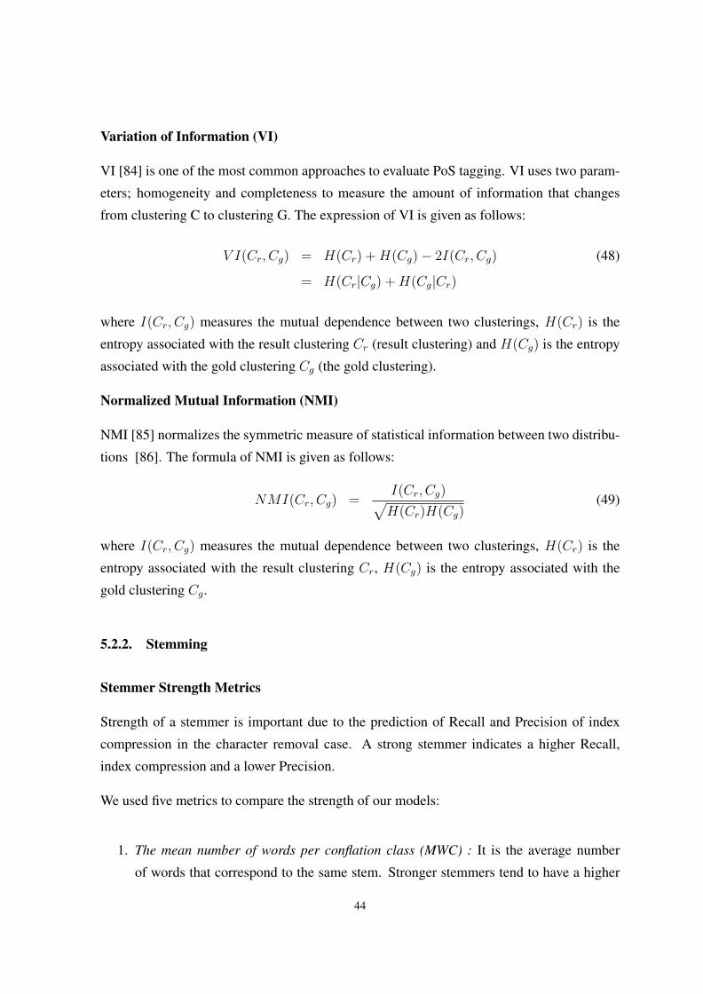
Variation of Information (VI)

VI [84] is one of the most common approaches to evaluate PoS tagging. VI uses two param-

eters; homogeneity and completeness to measure the amount of information that changes

from clustering C to clustering G. The expression of VI is given as follows:

V I(Cr, Cg) = H(Cr) +H(Cg)− 2I(Cr, Cg) (48)

= H(Cr|Cg) +H(Cg|Cr)

where I(Cr, Cg) measures the mutual dependence between two clusterings, H(Cr) is the

entropy associated with the result clustering Cr (result clustering) and H(Cg) is the entropy

associated with the gold clustering Cg (the gold clustering).

Normalized Mutual Information (NMI)

NMI [85] normalizes the symmetric measure of statistical information between two distribu-

tions [86]. The formula of NMI is given as follows:

NMI(Cr, Cg) =I(Cr, Cg)√H(Cr)H(Cg)

(49)

where I(Cr, Cg) measures the mutual dependence between two clusterings, H(Cr) is the

entropy associated with the result clustering Cr, H(Cg) is the entropy associated with the

gold clustering Cg.

5.2.2. Stemming

Stemmer Strength Metrics

Strength of a stemmer is important due to the prediction of Recall and Precision of index

compression in the character removal case. A strong stemmer indicates a higher Recall,

index compression and a lower Precision.

We used five metrics to compare the strength of our models:

1. The mean number of words per conflation class (MWC) : It is the average number

of words that correspond to the same stem. Stronger stemmers tend to have a higher

44

MWC. It is computed as given below:

MWC =N

S(50)

where S is the number of unique stems once the stemming is performed and N is total

number of unique words in the corpus.

2. Index compression factor (ICF) : It measures the decrease of the size of the corpus as

a result of stemming. This can be calculated by;

ICF =N − SN

(51)

where N is the number of unique words before stemming and N is the number of

unique words after stemming. Stronger stemmers tend to have a higher ICF.

3. The number of words and stems that differ (NWSF) : It is the difference between the

number of words before and after stemming. It indicates the strength of stemming

because stronger stemmers tend to transform words more than weaker stemmers.

4. The mean number of characters removed (MCRS) : It counts the number of characters

that are removed by the stemmer. Stronger stemmers tend to remove more characters

from words to obtain stems compared to weaker stemmers.

5. The mean and median Modified Hamming distance (MHD) : It measures the distance

between words and their stems. The modified Hamming distance is calculated by

adding the Hamming distance to the difference in the length between the word and its

stem.

Accuracy

Accuracy is used to measure the correctness of stems obtained at the end of stemming.

Frakes and Fox Similarity Metric (FSM)

This metric is proposed by Frakes and Fox [87] to evaluate the strength and similarity based

on the Hamming distance measure. It is calculated by;

Na =Nw

Ns

(52)

45

Na is the average number of words per conflation class, Nw refers to the number of unique

words before stemming, and Ns is the number of unique stems after stemming.

5.3. Experiments

We ran experiments for Turkish, English, Finnish, Hungarian and Basque. As defined in

Chapter 4., our models have four hyperparameters: α, β, γ and δ. We manually set these

hyperparameters for each experiment. We defined six sets for the values of the hyperparam-

eters.

1. set α=0.003 β=1 γ=0.003 δ=0.003

2. set α=0.003 β=0.1 γ=0.003 δ=0.003

3. set α=0.001 β=1 γ=0.001 δ=0.001

4. set α=0.001 β=0.1 γ=0.001 δ=0.001

5. set α=0.03 β=1 γ=0.03 δ=0.03

6. set α=0.03 β=0.1 γ=0.03 δ=0.03

The evaluation scores for each set will be given separately in order to understand the efforts

of hyperparameters better. For each experiment, we performed 5000 iterations in Gibbs

sampling.

We implemented our models on Python 3.5, and tested it on a server with Express x3650

M5, Xeon 6C E5-2620v3 2.4GHz/1866MHz/15MB Intel Xeon 2.40GHz processor. Training

Bayesian S-HMM and Bayesian SM-HMM models on 53K dataset takes about 15h, 24K

datasets about 8h, and 12K datasets about 6h. Bayesian SM-HMM. Training Bayesian CS-

HMM and Bayesian CSM-HMM models takes longer about 2-3h on datasets due to access

neural word embeddings obtained from word2vec [78] and finally Bayesian A-HMM and

Bayesian AS-HMM models on 53K dataset takes about 24h, 24K datasets about 18h, and

and 12K datasets about 12h.

We compare our PoS tagging results with Brown Clustering1 [14] and Anchor HMM2 [29]

and our stemming results with HPS3 [45], Morfessor FlatCat4 [88], and Linguistica5 [53].1Brown Clustering: http://www.cs.berkeley.edu/˜pliang/software/

brown-cluster-1.2.zip(Percy Liang)2Anchor HMM: https://github.com/karlstratos/anchor3HPS: http://liks.fav.zcu.cz/HPS/4Morfessor FlatCat: https://github.com/aalto-speech/flatcat5Linguistica: http://linguistica.uchicago.edu/

46

http://www.cs.berkeley.edu/~pliang/software/brown-cluster-1.2.zip

http://www.cs.berkeley.edu/~pliang/software/brown-cluster-1.2.zip

https://github.com/karlstratos/anchor

http://liks.fav.zcu.cz/HPS/

https://github.com/aalto-speech/flatcat

http://linguistica.uchicago.edu/

Table 5.2. shows the PoS tagging results for Turkish for six hyperparameter sets. For PoS

tagging task, in Many-to-one accuracy, Bayesian S-HMM gives better results and in other

metrics, Bayesian CSM-HMM model gives better results than the other models. When we

look at the results, generally results of Bayesian CSM-HMM are better for PoS tagging. This

shows that using suffixes and semantic features helps in PoS tagging. The overall PoS tag-

ging results show that Bayesian CSM-HMM outperforms both Brown Clustering [14], word-

based Bayesian HMM [7](baseline model), and Anchor HMM [29] for Turkish according to

both Many-to-one, One-to-one, NMI and VI measure.

Since Anchor HMM [29] evaluation is restricted, One-to-one, NMI and VI accuracy couldn’t

be computed.

In terms of the hyperparameter values, the results show that the sixth hyperparameter set

gives better results than the others (see Figure 5.2.).

0

10

20

30

40

50

60

70

BayesianHMM

Bayesian S-HMM

BayesianSM-HMM

BayesianCS-HMM

BayesianCSM-HMM

Bayesian A-HMM

BayesianAS-HMM

Man

y-to

-on

e A

ccu

racy

0

5

10

15

20

25

30

35

BayesianHMM

Bayesian S-HMM

BayesianSM-HMM

BayesianCS-HMM

BayesianCSM-HMM

Bayesian A-HMM

BayesianAS-HMM

On

e-to

-on

e A

ccu

racy

0

5

10

15

20

25

30

35

BayesianHMM

Bayesian S-HMM

BayesianSM-HMM

BayesianCS-HMM

BayesianCSM-HMM

Bayesian A-HMM

BayesianAS-HMM

NM

I

0

1

2

3

4

5

6

7

BayesianHMM

Bayesian S-HMM

BayesianSM-HMM

BayesianCS-HMM

BayesianCSM-HMM

BayesianA-HMM

BayesianAS-HMM

VI

Parameter set1

Parameter set2

Parameter set3

Parameter set4

Parameter set5

Parameter set6

Figure 5.2. Sensitivity of hyperparameter sets for PoS tagging performance in Turkish

The stemming results for Turkish are given in Table 5.3.. The results show that Bayesian

CS-HMM model generally gives better results in among the six hyperparameter sets. Our

results are far better than HPS [45], Morfessor FlatCat [88], and Linguistica [53] for Turkish.

Adding neural word embbedings to the model made a significant improvement. This may

lead this conclusion:semantic information about stem and word has an important impact on

stemming.

47

Table 5.2. Turkish PoS tagging results for different hyperparameter sets

Metu-Sabancı TreebankMany-to-one One-to-one NMI VI

1

Bayesian HMM 54.92 25.32 19.99 5.00Bayesian S-HMM 53.36 26.15 17.84 5.16Bayesian SM-HMM 58.07 27.80 29.35 4.34Bayesian CS-HMM 52.27 23.81 17.67 5.17Bayesian CSM-HMM 60.09 27.73 30.43 4.28Bayesian A-HMM 43.26 18.38 6.99 5.83Bayesian AS-HMM 37.03 9.64 0.13 6.30

2


3


4


5


6

Bayesian HMM 56.79 27.31 23.25 4.79Bayesian S-HMM 64.43 26.33 29.22 5.54Bayesian SM-HMM 56.43 28.65 29.39 4.40Bayesian CS-HMM 57.38 28.87 24.64 4.72Bayesian CSM-HMM 59.32 30.93 30.95 4.30Bayesian A-HMM 46.24 30.01 11.36 5.34Bayesian AS-HMM 37.03 9.13 0.12 6.30Brown Clustering 54.91 30.70 26.78 4.47Anchor HMM 58.82 - - -

48

Table 5.3. Turkish stemming results for different hyperparameter sets

Metu-Sabancı TreebankAccuracy ICF MWC NWSF MCRS MHD FSM

1

Bayesian S-HMM 47.55 -0.97 4.24 28048 1.24 1.21 0.77Bayesian SM-HMM 34.97 -1.17 3.16 34685 1.56 1.37 0.60Bayesian CS-HMM 57.31 -1.41 3.61 2284 1.32 1.18 0.72Bayesian CSM-HMM 39.51 -1.15 3.45 32180 1.42 1.27 0.66Bayesian A-HMM 37.49 -1.53 3.46 33366 1.43 1.31 0.66Bayesian AS-HMM 43.57 -0.72 5.03 30211 1.09 1.11 0.87

2

Bayesian S-HMM 47.51 -0.02 8.52 28124 1.27 1.28 0.76Bayesian SM-HMM 34.97 -1.78 3.16 34684 1.56 1.37 0.60Bayesian CS-HMM 57.76 -1.40 3.63 22627 1.30 1.17 0.73Bayesian CSM-HMM 40.55 -1.43 3.62 31605 1.38 1.24 0.68Bayesian A-HMM 39.15 -0.97 4.45 32495 1.39 1.31 0.68Bayesian AS-HMM 43.43 -.072 5.04 30279 1.09 1.10 0.87

3

Bayesian S-HMM 47.30 -0.97 4.42 28185 1.24 1.22 0.77Bayesian SM-HMM 34.97 -1.78 3.16 34684 1.56 1.37 0.60Bayesian CS-HMM 57.47 -1.43 3.59 22771 1.31 1.17 0.72Bayesian CSM-HMM 39.50 -1.56 3.43 32184 1.42 1.27 0.66Bayesian A-HMM 37.30 -1.57 3.41 33457 1.45 1.32 0.65Bayesian AS-HMM 43.22 -0.77 4.89 30377 1.11 0.86

4


5


6

Bayesian S-HMM 47.29 -0.02 8.51 28225 1.28 1.29 0.75Bayesian SM-HMM 34.96 -1.78 3.17 34687 1.56 1.37 0.60Bayesian CS-HMM 63.83 -0.50 5.83 19401 1.07 1.02 0.89Bayesian CSM-HMM 41.08 -1.37 3.71 31312 1.37 1.23 0.69Bayesian A-HMM 40.89 -0.60 5.46 31567 1.34 1.30 0.71Bayesian AS-HMM 44.40 -0.59 5.43 29756 1.08 1.10 0.88HPS 53.79 -0.80 4.82 24521 1.18 1.08 0.81Morfessor 52.06 -0.85 5.10 23311 1.10 1.23 0.77Linguistica 52.33 -0.90 5.02 24021 1.07 0.81 0.76

49

We give also a summary of the stemming results of Turkish in Figure 5.3..

0

10

20

30

40

50

60

70

Parameterset1

Parameterset2

Parameterset3

Parameterset4

Parameterset5

Parameterset6

Acc

ura

cy

-2

-1,5

-1

-0,5

0

Parameterset1

Parameterset2

Parameterset3

Parameterset4

Parameterset5

Parameterset6

ICF

0

2

4

6

8

10

Parameterset1

Parameterset2

Parameterset3

Parameterset4

Parameterset5

Parameterset6

MW

C

0

5000

10000

15000

20000

25000

30000

35000

40000

Parameterset1

Parameterset2

Parameterset3

Parameterset4

Parameterset5

Parameterset6

NW

SF

0

0,2

0,4

0,6

0,8

1

1,2

1,4

1,6

Parameterset1

Parameterset2

Parameterset3

Parameterset4

Parameterset5

Parameterset6

MH

D

0

0,2

0,4

0,6

0,8

1

FSM

Bayesian S-HMM

Bayesian SM-HMM

Bayesian CS-HMM

Bayesian CSM-HMM

Bayesian A-HMM

Bayesian AS-HMM

0

0,5

1

1,5

2

Parameterset1

Parameterset2

Parameterset3

Parameterset4

Parameterset5

Parameterset6

MC

RS

Figure 5.3. Sensitivity of parameter set for stemming performance of Turkish

The Figure 5.4. shows the relation of metrics. We can see that there is a reverse relationship

between ICF, MWC, FSM and NWSF, MCRS, MHD. It can be concluded that the Bayesian

CS-HMM model is acting stronger than the other models as a stemmer.

• Bayesian SM-HMM

• Bayesian A-HMM

• Bayesian CSM-HMM

• Bayesian AS-HMM

• Bayesian S-HMM

• Bayesian CS-HMM

-

Accuracy

+

NWSF

+

-

MHD

+

-

FSM

-

+

ICF

-

+

MWC

-

+

MCRS

+

-

Figure 5.4. Features summary of proposed model for Turkish

50

The PoS tagging results for Hungarian are presented in Table 5.4. (see 12K results in

Appendix C in Table 3.1.). The results show that Bayesian SM-HMM gives the highest

scores for both Hungarian datasets. Bayesian CSM-HMM results are also close to Bayesian

SM-HMM. We used a small dataset to train word2vec [78] in Hungarian. When we com-

pare the Bayesian CSM-HMM results with the Turkish results, the small training set for

word2vec [78] can be the reason of comparably low results of Bayesian-CSM HMM. This

shows that using semantic features has a high impact on PoS tagging.

The overall PoS tagging results show that Bayesian-SM model outperform Brown Cluster-

ing [14], word-based Bayesian HMM [7], and Anchor HMM [29] for Hungarian according

to Many-to-one, One-to-one, NMI, and VI measure.

When we compare the results of 12K and 24K datasets, it is seen that PoS tagging scores

increase, as the dataset size increases.

Figure 5.5. shows the correlation of the dataset size and PoS tagging performance for Hun-

garian. The best PoS tagging results are obtained from Bayesian SM-HMM. Thus, we choose

this model to analyze the affect of the size of the dataset.

0

10

20

30

40

50

60

Parameterset1

Parameterset2

Parameterset3

Parameterset4

Parameterset5

Parameterset6

Man

y-to

-on

e A

ccu

racy

Bayesian SM-HMM Hungarian 12k Bayesian SM-HMM Hungarian 24k

0

5

10

15

20

25

30

35

Parameterset1

Parameterset2

Parameterset3

Parameterset4

Parameterset5

Parameterset6

On

e-to

-on

e A

ccu

racy


0

5

10

15

20

25

30

35

Parameterset1

Parameterset2

Parameterset3

Parameterset4

Parameterset5

Parameterset6

NM

I


44,24,44,64,8

55,25,45,6

Parameterset1

Parameterset2

Parameterset3

Parameterset4

Parameterset5

Parameterset6

VI


Figure 5.5. Sensitivity of dataset for PoS performance of Hungarian

Table 5.5. shows stemming results for 24K for six hyperparameter sets (see 12K results in

Appendix C in Table 3.2.). Linguistica [53] results increase with the dataset size, whereas

51

Table 5.4. Hungarian24k PoS tagging results for different hyperparameter sets

UD Hungarian24k TreebankMany-to-one One-to-one NMI VI

1


2


3


4


5


6


52

our models’ results and HPS [45], Morfessor FlatCat [88] results are not. The best results

are obtained from Linguistica [53]. We get the best results from the Bayesian CS-HMM

model for stemming. This was the same for Turkish. Our results obtained from the Bayesian

CS-HMM model are close to HPS [45] and far better than Morfessor FlatCat [88].

Table 5.6. shows PoS tagging results for Finnish 24K datasets for six hyperparameter sets

(see 12K results in Appendix C in Table 3.3.). We get the highest scores in Many-to-one,

NMI, and VI scores from the Bayesian CSM-HMM model. The highest One-to-one accuracy

is obtained from Brown Clustering [14]. The results show that Bayesian SM-HMM and

Bayesian CSM-HMM results are very close. This may be because of the small training set

for word2vec [78] used for Bayesian CSM-HMM model.

Table 5.7. shows stemming results for Finnish 24K datasets for six hyperparameter sets (see

12K results in Appendix C in Table 3.4.). The best results are obtained from Linguistica [53].

Among our models, the highest scores are obtained from Bayesian CS-HMM model like the

other two agglutinative languages: Turkish and Hungarian. Our results are far better than the

results of the HPS [45] and Morfessor FlatCat [88].

Table 5.8. shows PoS tagging results for Basque 24K datasets for six hyperparameter sets

(see 12K results in Appendix C in Table 3.5.). The best results are obtained from Brown

Clustering [14]. The results obtained from 24k dataset shows that we get better result with

larger dataset. The scores obtained from Bayesian SM-HMM and Bayesian CSM-HMM are

very close to Brown Clustering [14] and Anchor HMM [29] for 24K dataset.

Table 5.9. shows stemming results for Basque 24K datasets for six hyperparameter sets (see

12K results in Appendix C in Table 3.6.). For 12K dataset, the best results are obtained from

Morfessor FlatCat [88]. However, results of HPS [45], Morfessor FlatCat [88], Linguis-

tica [53] and Bayesian CS-HMM are very close. In 24K dataset, the best results are obtained

from Linguistica [53]. It is seen that, our stemming results are not affected by the dataset

size.

Table 5.10. shows PoS tagging results for Penn 24K datasets for six hyperparameter sets

(see 12K results in Appendix C in Table 3.7.). The best results are obtained from Anchor

HMM [29] for Many-to-one accuracy. Brown Clustering [14] gives the highest for One-to-

one, NMI, VI scores. However, it is seen that Bayesian HMM [7] model is far more behind

the joint models.

53

Table 5.5. Hungarian24k stemming results for different hyperparameter sets

UD Hungarian24k TreebankAccuracy ICF MWC NWSF MCRS MHD FSM

1

Bayesian S-HMM 48.26 -0.23 3.17 12400 1.46 1.50 0.62Bayesian SM-HMM 41.18 -0.39 2.83 14047 0.77 0.83 1.15Bayesian CS-HMM 57.03 0.72 13.00 13994 2.29 2.32 0.42Bayesian CSM-HMM 41.99 0.16 4.69 12036 0.92 0.96 1.02Bayesian A-HMM 41.37 -0.33 2.93 14008 1.16 1.22 0.80Bayesian AS-HMM 42.19 -0.11 3.49 13744 1.54 1.59 0.62

2


3

Bayesian S-HMM 46.31 0.20 4.86 12876 1.82 1.86 0.53Bayesian SM-HMM 41.18 -0.39 2.83 14048 0.77 0.83 1.15Bayesian CS-HMM 56.17 0.17 4.75 10503 1.51 1.54 0.63Bayesian CSM-HMM 42.19 -0.39 2.83 13861 0.79 0.85 1.12Bayesian A-HMM 41.07 -0.09 3.56 14100 1.42 1.46 0.67Bayesian AS-HMM 42.18 -0.10 3.51 13804 1.55 1.60 0.62

4


5


6

Bayesian S-HMM 45.87 0.22 5.01 12976 1.83 1.87 0.53Bayesian SM-HMM 41.18 -0.39 2.83 14048 0.77 0.83 1.15Bayesian CS-HMM 56.36 0.18 4.78 10469 1.50 1.53 0.64Bayesian CSM-HMM 42.25 -0.38 2.86 13800 0.80 0.86 1.11Bayesian A-HMM 41.27 -0.02 3.80 14045 1.50 1.55 0.63Bayesian AS-HMM 42.45 -0.06 3.62 13709 1.57 1.62 0.61HPS 58.98 0.09 3.87 9784 0.93 0.98 1.00Morfessor 45.89 -3.20 3.87 12907 2.36 0.99 0.41Linguistica 70.12 0.32 3.87 7154 0.73 0.82 1.21

54

Table 5.6. Finnish24k PoS tagging results for different hyperparameter sets

Finnish24k TreebankMany-to-one One-to-one NMI VI

1


2


3


4


5


6


55

Table 5.7. Finnish24k stemming results for different hyperparameter sets

Finnish24k TreebankAccuracy ICF MWC NWSF MCRS MHD FSM

1


2


3


4


5


6

Bayesian S-HMM 24.10 0.27 4.54 18194 2.39 2.55 0.39Bayesian SM-HMM 26.42 -0.51 2.19 17603 0.98 1.43 0.68Bayesian CS-HMM 38.06 0.08 3.63 14846 1.90 2.15 0.45Bayesian CSM-HMM 27.61 -0.48 2.24 17318 1.00 1.44 0.68Bayesian A-HMM 24.75 -0.14 2.91 18025 1.74 2.02 0.48Bayesian AS-HMM 23.70 -0.07 3.09 18255 1.96 2.15 0.46HPS 27.18 -0.17 17984 1.75 1.2 1.98 0.58Morfessor 25.93 -0.34 18234 1.84 1.7 2.06 0.54Linguistica 45.40 0.37 3.32 13102 1.04 1.57 0.62

56

Table 5.8. Basque24k PoS tagging results for different hyperparameter sets

Basque24k TreebankMany-to-one One-to-one NMI VI

1


2


3


4


5


6


57

Table 5.9. Basque24k stemming results for different hyperparameter sets

Basque24k TreebankAccuracy ICF MWC NWSF MCRS MHD FSM

1


2

Bayesian S-HMM 31.85 0.10 5.89 16357 1.72 2.12 0.46Bayesian SM-HMM 33.55 -0.69 3.12 15923 0.88 1.30 0.71Bayesian CS-HMM 48.48 -0.03 5.07 12351 1.25 1.67 0.57Bayesian CSM-HMM 37.18 -0.62 3.25 15048 0.89 1.32 0.71Bayesian A-HMM 32.77 -0.49 3.51 16112 1.12 1.55 0.62Bayesian AS-HMM 31.75 -0.27 4.13 16364 1.42 1.83 0.53

3


4


5


6

Bayesian S-HMM 31.92 0.09 5.78 16334 1.69 2.10 0.47Bayesian SM-HMM 33.54 -0.69 3.12 15922 0.88 1.30 0.71Bayesian CS-HMM 48.72 -0.01 5.16 12299 1.24 1.67 0.57Bayesian CSM-HMM 37.27 -0.60 3.28 15029 0.90 1.32 0.71Bayesian A-HMM 32.28 -0.38 3.81 16237 1.23 1.65 0.58Bayesian AS-HMM 31.53 -0.19 4.38 16417 1.48 1.89 0.52HPS 50.06 0.24 5.24 11579 0.77 1.21 0.77Morfessor 55.50 -0.64 5.24 10723 1.06 1.16 0.66Linguistica 53.17 0.43 5.24 11211 0.92 1.39 0.68

58

Since the English stems are not covered in Penn Treebank [81], we were not able to evaluate

the English stemming results for this dataset.

Table 5.11. shows PoS tagging results for udEnglish 24K datasets for six hyperparameter

sets (see 12K results in Appendix C in Table 3.8.). It is seen that the results of these datasets

are very similar to the results on Penn Treebank [81].

Table5.12. shows stemming results for udEnglish 24K datasets for six hyperparameter sets

(see 12K results in Appendix C in Table 3.9.). The best results are obtained from Linguis-

tica [53]. However, Bayesian CS-HMM model is much better than HPS [45] and Morfessor

FlatCat [88].

Examples to correct and incorrect stems in all languages are given in Tables 5.13., 5.14.,

5.15., 5.16., and 5.17. respectively. The results show that our joint model can find common

endings, such as sı, a, mıstım in Turkish.

Table 5.13. Examples to correct and incorrect stems of Turkish

TurkishCorrect Incorrect

koca-sı hic-bir

tuhaf-# operasy-onunda

bil-miyor Grossm-an

duvar-a esleri-ni

anla-mıstım yirm-i

Table 5.14. Examples to correct and incorrect stems of Hungarian

HungarianCorrect Incorrect

tanar-ok pedi-g

fizetes-enek ide-i

bertabla-ber befagyasz-tott

az-# pedag-ogus

felada-kent emelle-t

59

Table 5.10. Penn 24K PoS tagging results for different hyperparameter sets

Penn 24K TreebankMany-to-one One-to-one NMI VI

1


2


3


4

Bayesian HMM 32.95 19.27 8.56 6.09Bayesian S-HMM 33.10 19.12 8.70 6.11Bayesian SM-HMM 48.10 33.02 28.26 4.65Bayesian CS-HMM 33.49 17.07 8.35 6.13Bayesian CSM-HMM 43.10 29.43 26.22 4.67Bayesian A-HMM 29.23 13.23 3.07 6.51Bayesian AS-HMM 28.98 10.51 .14 6.69

5


6


60

Table 5.11. udEnglish 24K PoS tagging results for different hyperparameter sets

udEnglish 24K TreebankMany-to-one One-to-one NMI VI

1


2


3


4


5


6


61

Table 5.12. udEnglish 24K stemming results for different hyperparameter sets

udEnglish 24K TreebankAccuracy ICF MWC NWSF MCRS MHD FSM

1


2


3


4


5


6

Bayesian S-HMM 49.30 0.11 6.86 12324 1.24 1.32 0.74Bayesian SM-HMM 47.82 -0.12 5.43 12650 0.52 0.61 1.58Bayesian CS-HMM 78.99 -0.01 6.04 5350 0.43 0.52 1.84Bayesian CSM-HMM 50.13 -0.006 6.07 12095 0.69 0.78 1.25Bayesian A-HMM 46.85 -0.11 5.47 12886 0.71 0.80 1.22Bayesian AS-HMM 45.54 -0.04 5.84 13198 1.16 1.24 0.79HPS 75.21 -0.02 6.00 6012 0.81 0.55 0.79Morfessor 63.05 -0.9 5.96 7048 0.72 0.78 1.02Linguistica 83.84 0.16 5.86 5040 0.69 0.83 1.17

62

Table 5.15. Examples to correct and incorrect stems of Finnish

FinnishCorrect Incorrect

niska+an sai+si

suomenmaa+# tann+e

pappila+ssa tul+ee

piste+tta kotii+n

valinta+nsa oll+a

Table 5.16. Examples to correct and incorrect stems of Basque

BasqueCorrect Incorrect

lortu-tako mas-a

gero-# mol-de

palestinar-rak ematen

lan-ean nahas-mendu

etxe-ra baldin-tzak

Table 5.17. Examples to correct and incorrect stems of English

EnglishCorrect Incorrect

respect-ed caus-ing

year-s troubl-e

of-# thir-d

rumour-s investme-nt

kill-ed opera-ting

5.4. Conclusion

We proposed six different models that learn PoS tags and stems jointly for agglutinative

languages. We did experiments Turkish, Finnish, Hungarian as agglutinative languages and

63

also Basque and English. We compared our PoS tagging and stemming results with other

models. We showed that especially Bayesian CSM-HMM outperforms other models for

POS tagging task and Bayesian CS-HMM outperforms other models for the stemming task.

64

6. CONCLUSION

6.1. Conclusion

In this thesis, we described the joint task of stemming and PoS tagging and presented six

different unsupervised Bayesian joint PoS tagging and stemming models for agglutinative

languages which extended the word-based Bayesian HMM model [7]. In agglutinative lan-

guages like Turkish, Finnish or Hungarian stemming and PoS tagging are crucial and con-

nected processes. Joint models reveals effect of stemming and PoS tagging on each other.

We did experiments on Turkish, Finnish, Hungarian, Basque and English. Results showed

that the models can be applicable on other languages as well, although they are proposed for

agglutinative languages.

The research questions are concluded accordingly:

• We showed joint learning of PoS tagging and stemming helps in both tasks in terms of

their performance.

• We compared our PoS tagging with the Baseline model which is word-based.The re-

sults show that using stems and affixes rather than words improve PoS tagging results.

Stemming results also improve in the joint task.

• Semantic information play an important role in this thesis as Schone and Jurafsky

(2000) [89], Brychcin and Konopik (2015) [45], and Narasimhan et al. (2015) [90]

demonstrated the value of semantic information on PoS tagging and morphology.

Our study makes a valuable contribution to the joint learning in the PoS tagging and stem-

ming literature. Our experiments provides two major additions. First, we show that using

stems instead of words for PoS tagging task is more suitable for agglutinative languages.

Learning stems reduces sparsity in PoS tagging task. Second, using semantic information

for PoS tagging and stemming helps improve the scores of both tasks (We hypothesize that

morhologically related words - stem and word - have semantic similarity. The similarity can

be calculated by embedding vectors of words [78].).

65

6.2. Future Research Directions

The proposed joint PoS tagging and stemming model is a fully unsupervised model and

can be applicable to any language. However, there are many problems left unsolved by

the proposed models in this thesis. Experiments prove that stemming is effective but that

is limited to only regular words. In other words, model cannot handle stemming irregular

words. For instance, if a suffix starts with a vowel in some disyllables, haplology can be

seen in Turkish (agız+ı← agzı). This can be overcome by adding operations as features that

describe the transformation of a word to another word to capture irregular words. Adding

mechanism to find stems of irregular words may bring higher accuracy than current models.

Applying the model for a high order NLP task such as Text Classification for an extrinsic

evaluation remains as another future work.

66

A APPENDIX : PoS TAGSET REDUCTION

In this appendix, we present PoS tagset reduction for used datasets based on universal PoS

tagset of Petrov et al. (2011) [2]. The reduced tagset for the Penn Treebank is given in Table

1.1., for the Finn Treebank in Table 1.2., for the UD Treebank for Basque, Hungarian and

English in Table 1.3., 1.4., 1.5. respectievly, and for the Metu-Sabancı Turkish Treebank in

Table 1.6..

Table 1.1. The mapping of the Universal tagset to the Penn Treebank tagset

Universal tagset Penn Treebank tagsetVERB VBP,VBD,VBG,VBN,VB,VBZ,MDPRON WP,PRP, PRP,WP

PUNCT (“),(,),-LRB-,-NONE-,-RRB-,(.),(:),(”),$PRT RP,TODET WDT,EX,PDT,DTNOUN NN,NNP,NNPS,NNSADV RB,RBR,WRB,RBSADJ JJ,JJSUNKNOWN FW,UHADP INNUM CDCONJ CC

Table 1.2. The mapping of the Universal tagset to the FinnTreeBank tagset

Universal tagset FinnTreeBank tagsetVERB VPRON PronPUNCT PunctPRT PcleDET DetNOUN NADV AdvADJ AUNKNOWN Symb, Foreign, InterjADP AdpNUM NumCONJ C

67

Table 1.3. The mapping of the Universal tagset to UD Basque TreeBank tagset

Universal tagset UD Basque TreeBank tagsetVERB VERB, AUXPRON PRONPUNCT PUNCTPRT PARTDET DETNOUN NOUN, PROPNADV ADVADJ ADJUNKNOWN SYM, INTJ, XADP ADPNUM NUMCONJ CONJ

Table 1.4. The mapping of the Universal tagset to UD Hungarian TreeBank tagset

Universal tagset UD Hungarian TreeBank tagsetVERB VERB, AUXPRON PRONPUNCT PUNCTPRT PARTDET DETNOUN NOUN, PROPNADV ADVADJ ADJUNKNOWN X, INTJADP ADPNUM NUMCONJ CONJ , SCONJ

68

Table 1.5. The mapping of the Universal tagset to UD English TreeBank tagset

Universal tagset UD English TreeBank tagsetVERB VERB, AUXPRON PRONPUNCT PUNCTPRT PARTDET DETNOUN NOUN, PROPNADV ADVADJ ADJUNKNOWN X, INTJ, SYMADP ADPNUM NUMCONJ CONJ , SCONJ

Table 1.6. The mapping of the Universal tagset to the Metu-Sabancı Turkish Treebank tagset

Universal tagset Metu-Sabancı Turkish Treebank tagset

NounNoun Pron,Noun Ins,Noun Nom,Noun Verb,Noun Loc,Noun Acc,Noun Abl,Noun Gen, Noun Dat,Noun Adj,Noun Num,Noun Pnon,Noun Postp,Noun Equ

Adj Adj Noun,Adj Verb,Adj,Adj Pron,Adj Postp,Adj NumAdv Adv Verb,Adv Adj,Adv Noun,AdvConj ConjDet DetInterj InterjQues QuesVerb Verb,Negp,Verb Noun,Verb Postp,Verb Adj,Verb Adv,Verb VerbPostp PostpNum NumPron Pron,Pron NounPunc Punc

69

B APPENDIX : Word2vec DATA

Word2vec dataIn this appendix, we present datasets used to learn distributred representations of words by

word2vec [78].

English : The corpus with first one billion characters from Wikipedia. (http://mattmahoney.

net/dc/text8.zip)

Finn Treebank [82]: It is a treebank that has approximately 19 000 sentences or sentence

fragments, and 162 000 word forms.

The Basque UD Treebank [83]: It is part of the Basque Dependency Treebank(BDT) [91].

The treebank consists of 8.993 sentences and 121.443 tokens.

The Hungarian UD Treebank [83]: It is derived from the Szeged Dependency Tree-

bank [92]. It contains 1299 sentences and 42.032 words.

Turkish Boun Corpus [93]: A web corpus for Turkish is composed of four subcorpora. It

has 423M words and 491M tokens.

70

http://mattmahoney.net/dc/text8.zip

http://mattmahoney.net/dc/text8.zip

C APPENDIX : RESULTS FOR 12K DATASETS

In this appendix, we present PoS tagging and stemming results for 12K datasets for six

hyperparameter sets.

Table 3.1. Hungarian12K PoS tagging results for different hyperparameter sets

UD Hungarian 12K TreebankMany-to-one One-to-one NMI VI

1


2


3


4


5


6


71

Table 3.2. Hungarian12k stemming results for different hyperparameter sets

UD Hungarian12k TreebankAccuracy ICF MWC NWSF MCRS MHD FSM

1


2


3


4


5


6


72

Table 3.3. Finnish 12K PoS tagging results for different hyperparameter sets

Finnish 12K TreebankMany-to-one One-to-one NMI VI

1


2


3


4


5


6


73

Table 3.4. Finnish 12K stemming results for different hyperparameter sets

Finnish 12K TreebankAccuracy ICF MWC NWSF MCRS MHD FSM

1


2


3


4


5


6


74

Table 3.5. Basque 12K PoS tagging results for different hyperparameter sets

Basque 12K TreebankMany-to-one One-to-one NMI VI

1


2


3


4


5


6


75

Table 3.6. Basque 12K stemming results for different hyperparameter sets

Basque 12K TreebankAccuracy ICF MWC NWSF MCRS MHD FSM

1


2


3


4


5


6

Bayesian S-HMM 32.95 0.003 4.03 8056 1.60 2.00 0.49Bayesian SM-HMM 33.49 -0.55 2.59 7977 0.88 1.31 0.71Bayesian CS-HMM 49.04 -0.08 3.68 6124 1.17 1.59 0.60Bayesian CSM-HMM 37.36 -0.47 2.73 7512 0.90 1.32 0.71Bayesian A-HMM 32.43 -0.29 3.10 8111 1.23 1.65 0.58Bayesian AS-HMM 31.36 -0.16 3.44 8238 1.45 1.87 0.53HPS 48.95 0.26 4.00 6153 0.81 1.26 0.74Morfessor 51.70 -0.50 4.00 5829 1.18 1.24 0.61Linguistica 52.75 0.38 4.00 5668 0.93 1.40 0.67

76

Table 3.7. Penn 12K PoS tagging results for different hyperparameter sets

Penn 12K TreebankMany-to-one One-to-one NMI VI

1


2


3


4


5


6


77

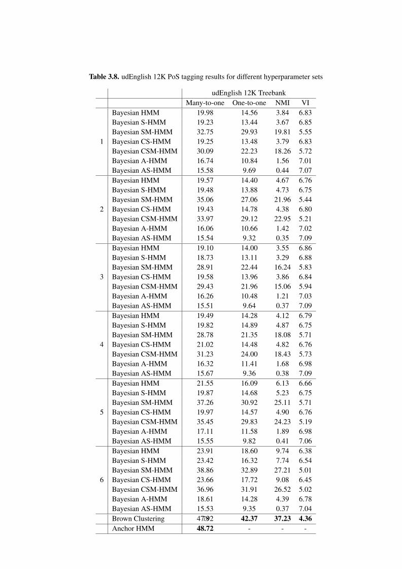
Table 3.8. udEnglish 12K PoS tagging results for different hyperparameter sets

udEnglish 12K TreebankMany-to-one One-to-one NMI VI

1


2


3


4


5


6


78

Table 3.9. udEnglish 12K stemming results for different hyperparameter sets

udEnglish 12K TreebankAccuracy ICF MWC NWSF MCRS MHD FSM

1


2

Bayesian S-HMM 50.83 -0.01 4.79 6044 1.15 1.23 0.80Bayesian SM-HMM 47.29 -0.10 4.37 6417 0.53 0.62 1.58Bayesian CS-HMM 79.71 -006 4.56 2645 0.39 0.47 2.02Bayesian CSM-HMM 49.75 -0.04 4.64 6121 0.67 0.75 1.29Bayesian A-HMM 46.05 -0.13 4.28 6567 0.75 0.84 1.16Bayesian AS-HMM 45.43 -0.11 4.34 6641 1.08 1.16 0.84

3


4


5


6

Bayesian S-HMM 51.19 0.01 4.89 5972 1.15 1.23 0.80Bayesian SM-HMM 47.29 -0.10 4.39 6417 0.53 0.62 1.57Bayesian CS-HMM 79.05 -0.04 4.64 2714 0.41 0.50 1.93Bayesian CSM-HMM 49.95 -0.06 4.82 6098 0.71 0.80 1.23Bayesian A-HMM 46.11 -0.11 4.35 6560 0.77 0.86 1.14Bayesian AS-HMM 44.91 -0.05 4.61 6699 1.17 1.25 0.78HPS 71.69 -0.15 4.65 3012 0.89 0.95 1.85Morfessor 64.74 -0.8 4.74 5142 1.02 1.02 1.46Linguistica 83.57 0.14 4.67 2514 0.69 0.83 1.17

79

REFERENCES

[1] Kairit Sirts and Tanel Alumae. A hierarchical dirichlet process model for joint

part-of-speech and morphology induction. In Proceedings of the 2012 Conference

of the North American Chapter of the Association for Computational Linguistics:

Human Language Technologies, pages 407–416. Association for Computational

Linguistics, 2012.

[2] Slav Petrov, Dipanjan Das, and Ryan McDonald. A universal part-of-speech

tagset. arXiv preprint arXiv:1104.2086, 2011.

[3] Robert Krovetz. Viewing morphology as an inference process. In Proceedings of

the 16th annual international ACM SIGIR conference on Research and develop-

ment in information retrieval, pages 191–202. ACM, 1993.

[4] Jorge Hankamer. Turkish generative morphology and morphological parsing. In

Second International Conference on Turkish Linguistics. Istanbul, Turkey. 1984.

[5] Yu Hu, Irina Matveeva, John Goldsmith, and Colin Sprague. Using morphology

and syntax together in unsupervised learning. In Proceedings of the Workshop

on Psychocomputational Models of Human Language Acquisition, pages 20–27.

Association for Computational Linguistics, 2005.

[6] Nicholas Ostler. Endangered Languages: What Role for the Specialist? Pro-

ceedings of the Foundation for Endangered Languages (FEL) Conference (2nd,

Edinburgh, Scotland, September 25-27, 1998). ERIC, 1998.

[7] Sharon Goldwater and Tom Griffiths. A fully Bayesian approach to unsuper-

vised part-of-speech tagging. In Annual meeting-association for computational

linguistics, volume 45, page 744. Citeseer, 2007.

[8] Jorge Hankamer. Morphological parsing and the lexicon. In Lexical representa-

tion and process, pages 392–408. MIT Press, 1989.

[9] Noam Chamsky. Aspects of the theory of syntax. Cambridge, Mass, 1965.

[10] Doug Cutting, Julian Kupiec, Jan Pedersen, and Penelope Sibun. A practical

part-of-speech tagger. In Proceedings of the third conference on Applied natural

80

language processing, pages 133–140. Association for Computational Linguistics,

1992.

[11] Adwait Ratnaparkhi et al. A maximum entropy model for part-of-speech tag-

ging. In Proceedings of the conference on empirical methods in natural language

processing, volume 1, pages 133–142. Philadelphia, USA, 1996.

[12] Ezra Black, Fred Jelinek, John Lafferty, Robert Mercer, and Salim Roukos. De-

cision tree models applied to the labeling of text with parts-of-speech. In Pro-

ceedings of the workshop on Speech and Natural Language, pages 117–121. As-

sociation for Computational Linguistics, 1992.

[13] Noah A Smith and Jason Eisner. Contrastive estimation: Training log-linear mod-

els on unlabeled data. In Proceedings of the 43rd Annual Meeting on Association

for Computational Linguistics, pages 354–362. Association for Computational

Linguistics, 2005.

[14] Peter F Brown, Peter V Desouza, Robert L Mercer, Vincent J Della Pietra, and

Jenifer C Lai. Class-based n-gram models of natural language. Computational

linguistics, 18(4):467–479, 1992.

[15] Steven Finch and Nick Chater. Bootstrapping syntactic categories using statis-

tical methods. Background and Experiments in Machine Learning of Natural

Language, 229:235, 1992.

[16] Alexander Clark. Inducing syntactic categories by context distribution clustering.

In Proceedings of the 2nd workshop on Learning language in logic and the 4th

conference on Computational natural language learning-Volume 7, pages 91–94.

Association for Computational Linguistics, 2000.

[17] Chris Biemann. Unsupervised part-of-speech tagging employing efficient graph

clustering. In Proceedings of the 21st international conference on computational

linguistics and 44th annual meeting of the association for computational linguis-

tics: student research workshop, pages 7–12. Association for Computational Lin-

guistics, 2006.

[18] Hinrich Schutze. Part-of-speech induction from scratch. In Proceedings of the

31st annual meeting on Association for Computational Linguistics, pages 251–

258. Association for Computational Linguistics, 1993.

81

[19] Hinrich Schutze. Distributional part-of-speech tagging. In Proceedings of the

seventh conference on European chapter of the Association for Computational

Linguistics, pages 141–148. Morgan Kaufmann Publishers Inc., 1995.

[20] Lawrence R Rabiner, CH Lee, BH Juang, and JG Wilpon. Hmm clustering for

connected word recognition. In Acoustics, Speech, and Signal Processing, 1989.

ICASSP-89., 1989 International Conference on, pages 405–408. IEEE, 1989.

[21] Bernard Merialdo. Tagging english text with a probabilistic model. Computa-

tional linguistics, 20(2):155–171, 1994.

[22] Michele Banko and Robert C Moore. Part of speech tagging in context. In Pro-

ceedings of the 20th international conference on Computational Linguistics, page

556. Association for Computational Linguistics, 2004.

[23] Mark Johnson. Why doesn’t em find good hmm pos-taggers? In EMNLP-CoNLL,

pages 296–305. 2007.

[24] Leonard E Baum, Ted Petrie, George Soules, and Norman Weiss. A maximization

technique occurring in the statistical analysis of probabilistic functions of markov

chains. The annals of mathematical statistics, 41(1):164–171, 1970.

[25] Stuart Geman and Donald Geman. Stochastic relaxation, gibbs distributions, and

the bayesian restoration of images. IEEE Transactions on pattern analysis and

machine intelligence, (6):721–741, 1984.

[26] David J.C. MacKay. Ensemble learning for hidden markov models. Technical

report, 1997.

[27] Jianfeng Gao and Mark Johnson. A comparison of bayesian estimators for unsu-

pervised hidden markov model pos taggers. In Proceedings of the Conference on

Empirical Methods in Natural Language Processing, pages 344–352. Association

for Computational Linguistics, 2008.

[28] Jurgen Van Gael, Andreas Vlachos, and Zoubin Ghahramani. The infinite hmm

for unsupervised pos tagging. In Proceedings of the 2009 Conference on Em-

pirical Methods in Natural Language Processing: Volume 2-Volume 2, pages

678–687. Association for Computational Linguistics, 2009.

82

[29] Karl Stratos, Michael Collins, and Daniel Hsu. Unsupervised part-of-speech tag-

ging with anchor hidden markov models. Transactions of the Association for

Computational Linguistics, 4:245–257, 2016.

[30] Christos Christodoulopoulos, Sharon Goldwater, and Mark Steedman. Two

decades of unsupervised pos induction: How far have we come? In Proceedings

of the 2010 Conference on Empirical Methods in Natural Language Processing,

pages 575–584. Association for Computational Linguistics, 2010.

[31] Aria Haghighi and Dan Klein. Prototype-driven learning for sequence models. In

Proceedings of the main conference on Human Language Technology Conference

of the North American Chapter of the Association of Computational Linguistics,

pages 320–327. Association for Computational Linguistics, 2006.

[32] Taylor Berg-Kirkpatrick, Alexandre Bouchard-Cote, John DeNero, and Dan

Klein. Painless unsupervised learning with features. In Human Language Tech-

nologies: The 2010 Annual Conference of the North American Chapter of the

Association for Computational Linguistics, pages 582–590. Association for Com-

putational Linguistics, 2010.

[33] Xipeng Qiu, F Eng Ji, Jiayi Zhao, and Xuanjing Huang. Joint segmentation and

tagging with coupled sequences labeling. 2012.

[34] Kairit Sirts, Jacob Eisenstein, Micha Elsner, Sharon Goldwater, et al. Pos

induction with distributional and morphological information using a distance-

dependent chinese restaurant process. In ACL (2), pages 265–271. 2014.

[35] Kemal Oflazer and Ilker Kuruoz. Tagging and morphological disambiguation of

turkish text. In Proceedings of the fourth conference on Applied natural language

processing, pages 144–149. Association for Computational Linguistics, 1994.

[36] Kemal Oflazer and Gokhan Tur. Morphological disambiguation by voting con-

straints. In Proceedings of the eighth conference on European chapter of the

Association for Computational Linguistics, pages 222–229. Association for Com-

putational Linguistics, 1997.

83

[37] Dilek Z Hakkani-Tur, Kemal Oflazer, and Gokhan Tur. Statistical morphologi-

cal disambiguation for agglutinative languages. In Proceedings of the 18th con-

ference on Computational linguistics-Volume 1, pages 285–291. Association for

Computational Linguistics, 2000.

[38] Levent Altunyurt, Zihni Orhan, and Tunga Gungor. A composite approach for

part of speech tagging in turkish. In Proceeding of International Scientific Con-

ference on Computer Science, Istanbul, Turkey. 2006.

[39] Taner Dincer, Bahar Karaoglan, and Tarik Kisla. A suffix based part-of-speech

tagger for turkish. In Information Technology: New Generations, 2008. ITNG

2008. Fifth International Conference on, pages 680–685. IEEE, 2008.

[40] Bi kent Universitfi. A tool for tagging turkish text.

[41] Julie B Lovins. Development of a stemming algorithm. 1968.

[42] John Dawson. Suffix removal and word conflation. ALLC bulletin, 2(3):33–46,

1974.

[43] Martin F Porter. An algorithm for suffix stripping. Program, 14(3):130–137,

1980.

[44] D Paice Chris et al. Another stemmer. In ACM SIGIR Forum, volume 24, pages

56–61. 1990.

[45] Tomas Brychcın and Miloslav Konopık. Hps: High precision stemmer. Informa-

tion Processing & Management, 51(1):68–91, 2015.

[46] Jiaul H Paik, Dipasree Pal, and Swapan K Parui. A novel corpus-based stemming

algorithm using co-occurrence statistics. In Proceedings of the 34th international

ACM SIGIR conference on Research and development in Information Retrieval,

pages 863–872. ACM, 2011.

[47] Jiaul H Paik, Mandar Mitra, Swapan K Parui, and Kalervo Jarvelin. Gras: An

effective and efficient stemming algorithm for information retrieval. ACM Trans-

actions on Information Systems (TOIS), 29(4):19, 2011.

84

[48] Jiaul H Paik, Swapan K Parui, Dipasree Pal, and Stephen E Robertson. Effective

and robust query-based stemming. ACM Transactions on Information Systems

(TOIS), 31(4):18, 2013.

[49] Prasenjit Majumder, Mandar Mitra, Swapan K Parui, Gobinda Kole, Pabitra Mi-

tra, and Kalyankumar Datta. Yass: Yet another suffix stripper. ACM transactions

on information systems (TOIS), 25(4):18, 2007.

[50] Zellig S Harris. From phoneme to morpheme. Language, 31(2):190–222, 1955.

[51] Jinxi Xu and W Bruce Croft. Corpus-based stemming using cooccurrence of

word variants. ACM Transactions on Information Systems (TOIS), 16(1):61–81,

1998.

[52] John Goldsmith. Unsupervised learning of the morphology of a natural language.

Computational linguistics, 27(2):153–198, 2001.

[53] John Goldsmith. An algorithm for the unsupervised learning of morphology.

Natural Language Engineering, 12(04):353–371, 2006.

[54] Michela Bacchin, Nicola Ferro, and Massimo Melucci. The effiectiveness of

a graph-based algorithm for stemming. In International Conference on Asian

Digital Libraries, pages 117–128. Springer, 2002.

[55] Massimo Melucci and Nicola Orio. A novel method for stemmer generation

based on hidden markov models. In Proceedings of the twelfth international

conference on Information and knowledge management, pages 131–138. ACM,

2003.

[56] Paul McNamee and James Mayfield. Character n-gram tokenization for european

language text retrieval. Information retrieval, 7(1-2):73–97, 2004.

[57] Michela Bacchin, Nicola Ferro, and Massimo Melucci. A probabilistic model

for stemmer generation. Information processing & management, 41(1):121–137,

2005.

[58] Jon M Kleinberg, Ravi Kumar, Prabhakar Raghavan, Sridhar Rajagopalan, and

Andrew S Tomkins. The web as a graph: measurements, models, and methods. In

International Computing and Combinatorics Conference, pages 1–17. Springer,

1999.

85

[59] Fuchun Peng, Nawaaz Ahmed, Xin Li, and Yumao Lu. Context sensitive stem-

ming for web search. In Proceedings of the 30th annual international ACM SI-

GIR conference on Research and development in information retrieval, pages

639–646. ACM, 2007.

[60] Jiaul H Paik and Swapan K Parui. A fast corpus-based stemmer. ACM Transac-

tions on Asian Language Information Processing (TALIP), 10(2):8, 2011.

[61] Manish Shrivastava, Nitin Agrawal, Bibhuti Mohapatra, Smriti Singh, and Push-

pak Bhattacharya. Morphology based natural language processing tools for in-

dian languages. In Proceedings of the 4th Annual Inter Research Institute Student

Seminar in Computer Science, IIT, Kanpur, India, April. Citeseer, 2005.

[62] A Goweder, H Alhami, Tarik Rashed, and A Al-Musrati. A hybrid method for

stemming arabic text. Journal of computer Science, URL: http://eref. uqu. edu.

sa/files/eref2/folder6/f181. pdf, 2008.

[63] Giorgos Adam, Konstantinos Asimakis, Christos Bouras, and Vassilis Poulopou-

los. An efficient mechanism for stemming and tagging: the case of greek lan-

guage. In International Conference on Knowledge-Based and Intelligent Infor-

mation and Engineering Systems, pages 389–397. Springer, 2010.

[64] Pratikkumar Patel Kashyap Popat and Pushpak Bhattacharyya. Hybrid stemmer

for gujarati. In 23rd International Conference on Computational Linguistics,

page 51. 2010.

[65] Kartik Suba Dipti Jiandani and Pushpak Bhattacharyya. Hybrid inflectional stem-

mer and rule-based derivational stemmer for gujarati. In Proceedings of the

2nd Workshop on South and Southeast Asian Natural Language Processing (WS-

SANLP 2011), page 1. 2011.

[66] Tarık KISLA and Bahar KARAOGLAN. A hybrid statistical approach to stem-

ming in turkish: An agglutinative language. Anadolu University of Sciences &

Technology-A: Applied Sciences & Engineering, 17(2), 2016.

[67] A Koksal. Bilgi erisim sorunu ve bir belge dizinleme ve erisim dizgesi tasarım

ve gerceklestirimi. ed: Yayınlanmamıs Docentlik Tezi, Hacettepe Universitesi,

Ankara, Turkey, 1979.

86

[68] Kemal Oflazer. Two-level description of turkish morphology. Literary and lin-

guistic computing, 9(2):137–148, 1994.

[69] Aysın Solak and Fazlı Can. Effects of stemming on turkish text retrieval. In

Proceedings of the Ninth Int. Symp. on Computer and Information Sciences (IS-

CIS’94), pages 49–56. 1994.

[70] Hayri Sever and Yıltan Bitirim. Findstem: Analysis and evaluation of a turk-

ish stemming algorithm. In International Symposium on String Processing and

Information Retrieval, pages 238–251. Springer, 2003.

[71] B Dincer and Bahar Karaoglan. Stemming in agglutinative languages: A prob-

abilistic stemmer for turkish. Computer and Information Sciences-ISCIS 2003,

pages 244–251, 2003.

[72] Gulsen Eryigit and Eref Adali. An affix stripping morphological analyzer for

turkish. In Proceedings of the IASTED International Conference on Artificial

Intelligence and Applications, Innsbruck, Austria, pages 299–304. 2004.

[73] Mehmet Dundar Akın and Ahmet Afsin Akın. Turk dilleri icin acık kaynaklı

dogal dil isleme kutuphanesi: Zemberek. Elektrik Muhendisligi, 431:38, 2007.

[74] Evren Kapusuz Cilden. Stemming turkish words using snowball, 2014.

[75] Muhammed Yavuz Nuzumlalı Arzucan Ozgur. Analyzing stemming approaches

for turkish multi-document summarization.

[76] Gunes Erkan and Dragomir R Radev. Lexrank: Graph-based lexical centrality

as salience in text summarization. Journal of Artificial Intelligence Research,

22:457–479, 2004.

[77] Ayberk Ozgur and BOUN EDU. An unsupervised stemming method for aggluti-

native languages.

[78] Tomas Mikolov, Ilya Sutskever, Kai Chen, Greg S Corrado, and Jeff Dean. Dis-

tributed representations of words and phrases and their compositionality. In Ad-

vances in neural information processing systems, pages 3111–3119. 2013.

[79] Gulsen Eryigit and Kemal Oflazer. Statistical dependency parsing of turkish.

2006.

87

[80] Kemal Oflazer, Bilge Say, Dilek Zeynep Hakkani-Tur, and Gokhan Tur. Building

a turkish treebank. Treebanks, pages 261–277, 2003.

[81] Mitchell P Marcus, Mary Ann Marcinkiewicz, and Beatrice Santorini. Building a

large annotated corpus of english: The penn treebank. Computational linguistics,

19(2):313–330, 1993.

[82] Atro Voutilainen, Tanja Purtonen, and Kristiina Muhonen. Outsourcing parse-

banking: The finntreebank project. In Shall We Play the Festschrift Game?, pages

117–131. Springer, 2012.

[83] Joakim Nivre, Marie-Catherine de Marneffe, Filip Ginter, Yoav Goldberg, Jan

Hajic, Christopher D Manning, Ryan McDonald, Slav Petrov, Sampo Pyysalo,

Natalia Silveira, et al. Universal dependencies v1: A multilingual treebank col-

lection. In Proceedings of the 10th International Conference on Language Re-

sources and Evaluation (LREC 2016), pages 1659–1666. 2016.

[84] Marina Meila. Comparing clusterings—an information based distance. Journal

of multivariate analysis, 98(5):873–895, 2007.

[85] Alexander Strehl and Joydeep Ghosh. Cluster ensembles—a knowledge reuse

framework for combining multiple partitions. Journal of machine learning re-

search, 3(Dec):583–617, 2002.

[86] Thomas M Cover and Joy A Thomas. Elements of information theory. John

Wiley & Sons, 2012.

[87] William B Frakes and Christopher J Fox. Strength and similarity of affix removal

stemming algorithms. In ACM SIGIR Forum, volume 37, pages 26–30. ACM,

2003.

[88] Stig-Arne Gronroos, Sami Virpioja, Peter Smit, and Mikko Kurimo. Morfessor

FlatCat: An HMM-based method for unsupervised and semi-supervised learning

of morphology. In COLING, pages 1177–1185. 2014.

[89] Patrick Schone and Daniel Jurafsky. Knowledge-free induction of inflectional

morphologies. In Proceedings of the second meeting of the North American

Chapter of the Association for Computational Linguistics on Language technolo-

gies, pages 1–9. Association for Computational Linguistics, 2001.

88

[90] Karthik Narasimhan, Regina Barzilay, and Tommi Jaakkola. An unsupervised

method for uncovering morphological chains. arXiv preprint arXiv:1503.02335,

2015.

[91] Itziar Aduriz et al. Construction of a basque dependency treebank. 2003.

[92] Veronika Vincze, Dora Szauter, Attila Almasi, Gyorgy Mora, Zoltan Alexin, and

Janos Csirik. Hungarian dependency treebank. In LREC, volume 10, pages 1855–

1862. Citeseer, 2010.

[93] Hasim Sak, Tunga Gungor, and Murat Saraclar. Turkish language resources:

Morphological parser, morphological disambiguator and web corpus. In GoTAL

2008, volume 5221 of LNCS, pages 417–427. Springer, 2008.

89

CURRICULUM VITAE

Credentials

Name,Surname: Necva BOLUCU

Place of Birth: Hatay,Turkey

Marital Status: Single

E-mail: [email protected]

Address: Computer Engineering Dept., Hacettepe University

Beytepe-ANKARA

EducationBSc. : ComputerEducation and Instructional Technology Dept.,

Cukurova University, Turkey

BSc. : Computer Engineering Dept., Mustafa Kemal University, Turkey

Foreign LanguagesEnglish

Work ExperienceComputer Teacher (2008-2015)

Research Assistant (2015-Present)

Areas of ExperiencesMachine Learning, NLP, Unsupervised Learning

Project and Budgets-

Oral and Poster Presentations-

PUBLICATIONS

Bolucu, N.,Can, B. ”Joint PoS Tagging and Stemming for Agglutinative Languages.” 18th In-

ternational Conference on Computational Linguistics and Intelligent Text Processing. 2016.90

Bolucu, Necva, Can, B. ”Stem-based PoS Tagging for Agglutinative Languages.” Signal

Processing and Communication Application Conference (SIU), 2017 25th. IEEE. 2016.

91

Scanned by CamScanner

unsupervised joint part-of-speech tagging ...burcucan/necvabolucu...unsupervised joint...

Documents