unsupervised audio feature extraction for music similarity ...jan.schlueter/pubs/msc.pdf · there...

Technische Universität MünchenFakultät für Informatik

Master’s Thesis in Informatics

Unsupervised Audio Feature Extractionfor Music Similarity Estimation

Jan Schlüter

Technische Universität MünchenFakultät für Informatik

Master’s Thesis in Informatics

Unsupervised Audio Feature Extractionfor Music Similarity Estimation

Ein Musikähnlichkeitsmaß auf Basisunüberwacht gelernter Audiomerkmale

Jan Schlüter

Supervisor:Prof. Dr. Alois Knoll

Advisor:Dipl.-Inf. Christian Osendorfer

October 8, 2011

There is a theory which states that if ever anybody discovers exactly what theUniverse is for and why it is here, it will instantly disappear and be replaced bysomething even more bizarre and inexplicable. There is another theory which statesthat this has already happened.

Douglas Adams

Declaration of OriginalityI assure the single handed composition of this master’s thesis only supported bydeclared resources.

EigenständigkeitserklärungIch versichere, dass ich diese Masterarbeit selbständig verfasst und nur die angegebe-nen Quellen und Hilfsmittel verwendet habe.

Wien, den Unterschrift:

V

AcknowledgementsForemost, I would like to thank Christian Osendorfer for introducing me to the artof machine learning at the Technical University of Munich, for giving me the oppor-tunity to work on Music Information Retrieval, and for pointing me to mcRBMsbefore I had even understood RBMs. I am also grateful to Breno Faria, with whomI enjoyed studying probabilities and likelihoods, priors and posteriors, classificationand regression, kernel tricks and feature spaces, NumPy and SciPy, Büchi and vanEmde Boas, top-fermented and bottom-fermented beer.Furthermore, I wish to thank Prof. Gerhard Widmer for calling me to Vienna

for a first project while I was in the thick of writing up this thesis, then giving methe time I needed to finish it. I am already looking forward to pursuing furtherresearch in the realms of machine learning with music at the OFAI – and even towriting the next thesis!Finally, I want to thank my parents for supporting me in all my endeavors, even if

they drove me farther and farther away from home, and my friends and my brother,who never let me down.

VII

Abstract

Fostered by the constant advancement of digital technologies, both catalogs of musicdistributors and personal music collections have grown to sizes that call for auto-mated methods to manage them. In this context, music similarity estimation playsan important role: It can be used to recommend music based on examples, to orga-nize a collection into groups, or to generate well-sounding playlists. Content-basedmethods are especially interesting in that they rely on sound only, not requiringany metadata.Most existing content-based music similarity estimation methods build on com-

plex hand-crafted feature extractors, which are difficult to engineer. As an alterna-tive, unsupervised machine learning allows to learn features empirically from data.Based on a review of existing approaches to music similarity estimation and relatedtasks in three other domains of pattern recognition, we design a music similarityestimation system based on unsupervisedly learned audio features.In particular, we train a recently proposed generative model, the mean-covariance

Restricted Boltzmann Machine (mcRBM), on music spectrogram excerpts and em-ploy it for feature extraction. In experiments on three public datasets, it clearlyoutperforms classic MFCC-based methods, surpasses simple unsupervised featureextraction using basic RBMs or k-Means and comes close to the state-of-the-art.This shows that unsupervised feature extraction poses a viable alternative to engi-neered features.

Zusammenfassung

Begünstigt durch die stetige Weiterentwicklung digitaler Technologien haben sowohldas Angebot der Musikhändler als auch persönliche Musiksammlungen inzwischenGrößen erreicht, die ohne automatische Methoden kaum zu handhaben sind. Musik-ähnlichkeitsmaße spielen in diesem Zusammenhang eine wichtige Rolle: Sie könnendazu verwendet werden, Musik auf Basis von Beispielen zu empfehlen, eine Samm-lung in Gruppen aufzuteilen, oder wohlklingende Wiedergabelisten zu generieren.Inhaltsbasierte Methoden sind besonders interessant, da sie ausschließlich auf demKlang aufbauen und keine Metadaten benötigen.Die meisten existierenden inhaltsbasierten Musikähnlichkeitsmaße basieren auf

komplizierten, von Hand erstellten Merkmalsextraktoren, die schwierig zu entwi-ckeln sind. Eine Alternative bieten unüberwachte maschinelle Lernmethoden, dieMerkmale empirisch aus Daten lernen können. Ausgehend von einer Begutachtungexistierender Musikähnlichkeitsmaße sowie dazu verwandter Methoden aus drei an-deren Gebieten der Mustererkennung entwickeln wir ein Musikähnlichkeitsmaß aufBasis unüberwacht gelernter Audiomerkmale.

IX

Insbesondere trainieren wir ein vor kurzem entwickeltes generatives Modell, diemean-covariance Restricted Boltzmann Machine (mcRBM), auf Auschnitten ausMusikspektrogrammen und setzen es zur Merkmalsextraktion ein. In Experimentenauf drei frei verfügbaren Datensätzen ist es klassischen MFCC-basierten Ansätzenklar überlegen, übertrifft einfachere unüberwachte Merkmalsextraktion mit gewöhn-lichen RBMs oder k-Means und kommt nahe an den aktuellen Stand der Technik.Das zeigt, dass unüberwachte Merkmalsextraktion eine praktikable Alternative zuvon Hand entwickelten Features darstellt.

X

Contents

List of Figures XV

List of Tables XVII

1 Introduction 11.1 Content-based music similarity estimation – what for? . . . . . . . . 1

1.1.1 Automated music recommendation . . . . . . . . . . . . . . . 11.1.2 Established music recommendation systems . . . . . . . . . . 21.1.3 Use of content-based music similarity estimation . . . . . . . 3

1.2 Unsupervised Machine Learning for Feature Extraction . . . . . . . 51.2.1 Hand-Crafting vs. Machine Learning . . . . . . . . . . . . . . 51.2.2 Unsupervised Feature Extraction . . . . . . . . . . . . . . . . 6

1.3 Thesis Outline . . . . . . . . . . . . . . . . . . . . . . . . . . . . . . 6

2 Existing Content-based Music Similarity Measures 92.1 General Scheme . . . . . . . . . . . . . . . . . . . . . . . . . . . . . . 92.2 Classic Approach: GMMs of MFCCs . . . . . . . . . . . . . . . . . . 11

2.2.1 Local Features: Mel-Frequency Cepstral Coefficients . . . . . 112.2.2 Global Model: Gaussian Mixture Model . . . . . . . . . . . . 142.2.3 Distance Measure: Kullback-Leibler Divergence . . . . . . . . 142.2.4 Shortcomings of this Method . . . . . . . . . . . . . . . . . . 15

2.3 Advancements and Alternatives . . . . . . . . . . . . . . . . . . . . . 182.3.1 Global Models and Distance Functions . . . . . . . . . . . . . 192.3.2 Short-term Local Features . . . . . . . . . . . . . . . . . . . . 242.3.3 Long-term Local Features . . . . . . . . . . . . . . . . . . . . 252.3.4 Combined Features . . . . . . . . . . . . . . . . . . . . . . . . 27

2.4 Conclusions . . . . . . . . . . . . . . . . . . . . . . . . . . . . . . . . 28

3 Inspiration from other Domains of Pattern Recognition and InformationRetrieval 313.1 Text Retrieval Systems . . . . . . . . . . . . . . . . . . . . . . . . . . 313.2 Computer Vision Systems . . . . . . . . . . . . . . . . . . . . . . . . 373.3 Speech Processing Systems . . . . . . . . . . . . . . . . . . . . . . . 433.4 Conclusions . . . . . . . . . . . . . . . . . . . . . . . . . . . . . . . . 46

XI

Contents

4 Proposed New Method 474.1 The Big Picture . . . . . . . . . . . . . . . . . . . . . . . . . . . . . . 474.2 Local Feature Extraction . . . . . . . . . . . . . . . . . . . . . . . . 484.3 Preprocessing . . . . . . . . . . . . . . . . . . . . . . . . . . . . . . . 53

4.3.1 Whitening . . . . . . . . . . . . . . . . . . . . . . . . . . . . . 534.3.2 Compression . . . . . . . . . . . . . . . . . . . . . . . . . . . 59

4.4 Feature Abstraction . . . . . . . . . . . . . . . . . . . . . . . . . . . 614.4.1 Restricted Boltzmann Machines (RBMs) . . . . . . . . . . . . 614.4.2 Mean-Covariance Restricted Boltzmann Machines (mcRBMs) 684.4.3 Deep Belief Nets (DBNs) . . . . . . . . . . . . . . . . . . . . 754.4.4 Mini-batch k-Means++ . . . . . . . . . . . . . . . . . . . . . 77

4.5 Global Modeling . . . . . . . . . . . . . . . . . . . . . . . . . . . . . 804.6 Song Comparison . . . . . . . . . . . . . . . . . . . . . . . . . . . . . 81

4.6.1 Distance Measures . . . . . . . . . . . . . . . . . . . . . . . . 814.6.2 Distance Space Normalization . . . . . . . . . . . . . . . . . . 83

5 Experimental Evaluation 855.1 Evaluating Music Similarity Measures . . . . . . . . . . . . . . . . . 85

5.1.1 The Quest for Ground Truth . . . . . . . . . . . . . . . . . . 865.1.2 Available Datasets . . . . . . . . . . . . . . . . . . . . . . . . 88

5.2 Chosen Evaluation Approaches . . . . . . . . . . . . . . . . . . . . . 895.3 Results on Decorrelating Musical Spectra . . . . . . . . . . . . . . . 92

5.3.1 Visual Comparison . . . . . . . . . . . . . . . . . . . . . . . . 935.3.2 Effects on Music Similarity Estimation . . . . . . . . . . . . . 96

5.4 Stepwise Evaluation of the New System . . . . . . . . . . . . . . . . 1005.4.1 Lower bound, Baseline and State-of-the-art . . . . . . . . . . 1005.4.2 Frame-wise Gaussian Mixture Models . . . . . . . . . . . . . 1035.4.3 Frame-wise k-Means Histograms . . . . . . . . . . . . . . . . 1045.4.4 Frame-wise (mc)RBM Histograms . . . . . . . . . . . . . . . 1095.4.5 Block-wise Single Gaussian Models . . . . . . . . . . . . . . . 1115.4.6 Block-wise k-Means Histograms . . . . . . . . . . . . . . . . . 1135.4.7 Block-wise (mc)RBM Histograms . . . . . . . . . . . . . . . . 1155.4.8 Distance Space Normalization . . . . . . . . . . . . . . . . . . 1265.4.9 Cross-Dataset Generalization . . . . . . . . . . . . . . . . . . 128

5.5 Final Comparison . . . . . . . . . . . . . . . . . . . . . . . . . . . . . 1295.5.1 Retrieval Precision and Classification Accuracy . . . . . . . . 1295.5.2 Genre Confusion . . . . . . . . . . . . . . . . . . . . . . . . . 1305.5.3 Hubness . . . . . . . . . . . . . . . . . . . . . . . . . . . . . . 1325.5.4 Summary . . . . . . . . . . . . . . . . . . . . . . . . . . . . . 136

XII

Contents

6 Conclusion 1396.1 Recapitulation . . . . . . . . . . . . . . . . . . . . . . . . . . . . . . 1396.2 Future Work . . . . . . . . . . . . . . . . . . . . . . . . . . . . . . . 140

A Derivations for Restricted Boltzmann Machines 143A.1 Conditional probabilities . . . . . . . . . . . . . . . . . . . . . . . . . 143A.2 Likelihood Gradient . . . . . . . . . . . . . . . . . . . . . . . . . . . 144

Bibliography 147

XIII

List of Figures

2.1 Common architecture of content-based music similarity estimationsystems . . . . . . . . . . . . . . . . . . . . . . . . . . . . . . . . . . 10

4.1 Block diagram for the proposed music similarity estimation system . 484.2 Plots of two mel filter banks . . . . . . . . . . . . . . . . . . . . . . . 514.3 The local feature extraction process interpreted as computing a spec-

trogram, mapping it to the mel scale and extracting patches. . . . . 524.4 PCA and ZCA whitening of 2D observations . . . . . . . . . . . . . 574.5 PCA and ZCA whitening filters and dewhitening filters for mel-

spectral blocks, as well as whitened data . . . . . . . . . . . . . . . . 584.6 A Restricted Boltzmann Machine (RBM) . . . . . . . . . . . . . . . 614.7 Illustration of blocked Gibbs sampling . . . . . . . . . . . . . . . . . 654.8 Contrastive Divergence compared to Persistent Contrastive Divergence 694.9 Diagrams of the two parts of a mean-covariance RBM. . . . . . . . . 704.10 Reconstruction of a music excerpt with mean units or mean and

covariance units of an mcRBM . . . . . . . . . . . . . . . . . . . . . 744.11 A Deep Belief Network (DBN) composed of three RBMs. . . . . . . 76

5.1 Covariance and principal components for mel-spectral frames com-pared to a Toeplitz matrix and its principal components . . . . . . . 94

5.2 Lower bound, “Single Gaussian of MFCCs” and state-of-the-art re-sults on all three evaluation datasets . . . . . . . . . . . . . . . . . . 102

5.3 Random excerpt of a codebook learned by k-Means on 1517-Artists . 1075.4 Examples of (mc)RBM filters learned on 1517-Artists . . . . . . . . 1115.5 Exemplary codebook entries learned by k-Means on mel-spectral

blocks of different lengths and compressions . . . . . . . . . . . . . . 1145.6 Illustration of a topographic mcRBM factor-to-hidden pooling matrix 1175.7 Exemplary filters learned by mcRBMs on mel-spectral blocks of dif-

ferent lengths and datasets . . . . . . . . . . . . . . . . . . . . . . . 1245.8 Our best models compared to the baseline and state-of-the-art on all

three evaluation datasets . . . . . . . . . . . . . . . . . . . . . . . . . 1315.9 Confusion matrices for the baseline, our method and the state-of-

the-art on 1517-Artists and Ballroom . . . . . . . . . . . . . . . . . . 133

XV

List of Figures

5.10 k-occurrence histograms and skewness for two baselines, our methodand the state-of-the-art on 1517-Artists . . . . . . . . . . . . . . . . 135

XVI

List of Tables

5.1 Precision at k for several variations of mel-spectral features modeledby full-covariance Gaussians . . . . . . . . . . . . . . . . . . . . . . . 97

5.2 Repetition of the previous experiment with diagonal-covariance Gaus-sians . . . . . . . . . . . . . . . . . . . . . . . . . . . . . . . . . . . . 98

5.3 Repetition of the previous experiments with a mean-only model andEuclidean distance . . . . . . . . . . . . . . . . . . . . . . . . . . . . 99

5.4 Lower bound, “Single Gaussian of MFCCs” and state-of-the-art re-sults on all three evaluation datasets . . . . . . . . . . . . . . . . . . 101

5.5 Gaussian Mixture Models evaluated on frame-wise features of 1517-Artists . . . . . . . . . . . . . . . . . . . . . . . . . . . . . . . . . . . 104

5.6 Comparison of different distance measures for k-Means histogrammodels . . . . . . . . . . . . . . . . . . . . . . . . . . . . . . . . . . . 105

5.7 Comparison of different codebook sizes for k-Means histogram models1065.8 Comparison of different feature preprocessings for k-Means histogram

models . . . . . . . . . . . . . . . . . . . . . . . . . . . . . . . . . . . 1075.9 Results for the best frame-wise k-Means histogram model on all three

datasets compared to three other approaches. . . . . . . . . . . . . . 1085.10 Results for (mc)RBM histogrammodels on PCA-whitened log-magnitude

mel-spectral frames of 1517-Artists. . . . . . . . . . . . . . . . . . . . 1105.11 Results for single Gaussian models on mel-spectral blocks of 1517-

Artists . . . . . . . . . . . . . . . . . . . . . . . . . . . . . . . . . . . 1125.12 Results for k-Means histogram models on mel-spectral blocks of 1517-

Artists . . . . . . . . . . . . . . . . . . . . . . . . . . . . . . . . . . . 1135.13 Results for the best block-wise k-Means histogram model on all three

datasets compared to three other approaches. . . . . . . . . . . . . . 1145.14 Results for mRBM histogram models on mel-spectral blocks of 1517-

Artists . . . . . . . . . . . . . . . . . . . . . . . . . . . . . . . . . . . 1165.15 Results for different mcRBM architectures on mel-spectral blocks of

1517-Artists . . . . . . . . . . . . . . . . . . . . . . . . . . . . . . . . 1185.16 Comparison of different feature preprocessings for block-wise mcRBM

histogram models . . . . . . . . . . . . . . . . . . . . . . . . . . . . . 1195.17 Comparison of different block sizes for mcRBM histogram models . . 1205.18 Comparison of different DBN histogram models on mel-spectral blocks121

XVII

List of Tables

5.19 Comparison of unit-wise and combination-wise histogramming of la-tent representations of spectral blocks. . . . . . . . . . . . . . . . . . 122

5.20 Results for the best block-wise mcRBM histogram models on all threedatasets compared to three other approaches. . . . . . . . . . . . . . 125

5.21 Results for the best models on all three datasets with and withoutDistance Space Normalization (DSN), compared to the state-of-the-art.127

5.22 Cross-dataset generalization of mcRBM histogram models . . . . . . 1285.23 Our best models compared to the baseline and state-of-the-art on all

three evaluation datasets. . . . . . . . . . . . . . . . . . . . . . . . . 130

XVIII

1 Introduction

Nowadays, music gets produced and published at a higher rate than any individualcan listen to it: Estimates reach from a yearly “11,000 (nonclassical) major labelalbums averaging some ten cuts per album” [Vog04, p. 261] up to 97,751 albumsreleased in the United States in 2009, as reported by Nielsen SoundScan1.In this chapter, we will explain that this creates a need for automatic music

recommendation systems, motivate how content-based music similarity estimationwould help in this context and point out further useful applications, briefly reasonwhy unsupervised machine learning methods are appealing for this task and finishwith an outline of the main parts of this thesis.

1.1 Content-based music similarity estimation – what for?

1.1.1 Automated music recommendation

According to the estimations given above, the corpus of available music is growingat an extraordinary rate of possibly over five hours of newly released music per hour.As a consequence, any music listener has to rely on filters to provide a selectionof music she or he likes. A listener looking for new music traditionally only hadlimited influence on these filters, such as by choosing a radio station to listen toor a shelve in a music store to look through, and was largely dependant on others’choices, such as the station’s editorial’s decisions on the playlist, or the selectionand sorting of records by staff in the store.Digital technologies have changed this situation in at least two respects: Digital

music distribution channels such as iTunes or Amazon can provide quick access tomillions of music pieces with low expenses, so they are less strictly filtered, and,with the abandonment of physical records, they shifted granularity from albums tosingle tracks, making it even harder for potential customers to make a choice. To fillin this gap of missing filters, automatic music recommendation systems have arisen,attempting to provide highly individually targeted access to the world’s music.

1http://www.billboard.biz/bbbiz/content_display/industry/news/e3i4ad94ea6265fac02d4c813c0b6a93ca2

1

http://www.billboard.biz/bbbiz/content_display/industry/news/e3i4ad94ea6265fac02d4c813c0b6a93ca2

http://www.billboard.biz/bbbiz/content_display/industry/news/e3i4ad94ea6265fac02d4c813c0b6a93ca2

1 Introduction

1.1.2 Established music recommendation systemsAn informal study among university students (aged 20 to 25, German or Austrian,experienced Internet users, but not familiar with Music Information Retrieval, Sig-nal Processing or Computer Science) resulted in a list of six Internet platforms thatare commonly associated with music recommendation. In the following, we willbriefly review how these systems work to show in which respect industry’s state-of-the-art still falls short of satisfyingly solving the problem at hands. See [Sca09,pp. 9–15] for an alternative and more extensive review of some of these services.

Amazon suggests albums or songs based on what has been purchased in the sameorder or by the same customers as items one searched for or bought. This is aform of collaborative filtering [HKBR99], which assumes that users who haveagreed in the past (in their purchase decisions) will also agree in the future(by purchasing the same items).Collaborative filtering generally suffers from two related problems: The cold-start problem and the popularity bias. In this case, the former means thatalbums that have not yet been purchased by anybody can never be suggested,and the latter describes that for any given item, popular albums are morelikely to have been purchased in conjunction with it than unpopular ones, andso have a better chance of being recommended. In consequence, collaborativefiltering is incapable of suggesting new music releases. An additional problemspecific to Amazon is that users may purchase items for somebody else (e.g.,as a present), which will flaw the recommendations generated both for themand for other users of allegedly the same taste.

Spotify, a music streaming service, bases its recommendations on its users’ listeningbehavior, analyzing which artists are often played by the same listeners. Whilethis may potentially result in better suggestions than analyzing sparse datasuch as record purchases, it is again subject to the cold-start problem andpopularity bias. Furthermore, Spotify only recommends related artists, whichis rather unspecific.

Genius is a function in Apple iTunes which generates playlists and song recom-mendations by comparing music libraries, purchase histories and playlists ofall its users, possibly integrating external sources of information. Assumingsuch external information does not play a major role, this system is based oncollaborative filtering and will suffer from its problems.

Last.fm combines information obtained from users’ listening behavior and user-supplied tags (words or short expressions describing a song or artist). Whiletags can help making recommendations transparent to users – e.g., a user lis-tening to a love song may be suggested other tracks that have frequently been

2

1.1 Content-based music similarity estimation – what for?

tagged as “slow” and “romantic” – they are easily manipulated by malicioususers, requiring counter measures [LFZ09], and are affected by the cold-startproblem and popularity bias.

Pandora, another music streaming service, recommends songs from its catalogbased on expert reviews of tracks with respect to a few hundred genre-specificcriteria. This allows very accurate suggestions of songs that sound similar towhat a user listens to, including sophisticated explanations for why a songwas suggested – e.g., a track may be recommended because it is in “majorkey”, features “acoustic rhythm guitars”, “a subtle use of vocal harmony” andexhibits “punk influences” 2. As it is based on analyzing the musical contentrather than collaborative filtering of users’ consumption or unrestricted tagdescriptions, it is not affected by the popularity bias. However, the expertreviews incur high costs in terms of time and money: An annotation time of45 minutes per track [Sca09, p. 45] makes it infeasible to extend the catalogat a rate that can keep up with new releases, limiting the selection of musicavailable to users similarly to the cold-start problem.

Shazam has often been named as well. While it analyzes the sound of music tracks,the original Shazam service actually does not provide any recommendations,but only finds the exact same track in its database to provide the user withmetadata such as the artist or title of the song. The audio features extractedby the system (constellations of peaks in the spectrogram [Wan03]) are tai-lored to solving this task under very noisy conditions, but not useful for findingand recommending songs that sound similar rather than identical.

1.1.3 Use of content-based music similarity estimation

1.1.3.1 Large-scale recommendation

Despite these recommendation systems, only a small fraction of new albums attracta wider audience: According to Nielsen SoundScan, only 2.1% of 2009’s releases soldmore than 5,000 copies, and 12 releases (0.01%) sold more than a million. Albumsales thus follow what is commonly known as a Power Law (or Pareto) distribution,where very few items sell very well, while the other items remain in the Long Tailand hardly sell at all [And06]. This means that either an overwhelming majority oftoday’s music sounds bad, or a lot of good music still never gets found by interestedlisteners (or a combination of both).We assume that at least two factors contribute to the latter: Firstly, music

recommendation systems are not yet widespread enough to dominate album sale2song description from http://www.pandora.com/music/song/shins/kissing+lipless

3

http://www.pandora.com/music/song/shins/kissing+lipless

1 Introduction

statistics, and secondly, all common systems except for Pandora are based on col-laborative filtering and are thus susceptible to popularity bias, which encourages aPareto distribution rather than giving users easy access to the Long Tail.Revealing music pieces hidden in the Long Tail that suit the taste of a user seem-

ingly needs a recommendation system that is not based on collaborative filtering.While Pandora is such a system, it requires costly experts and so can only handle alimited catalog of music. Audio content-based music similarity estimation attemptsto automate the process of listening to music pieces and inferring information abouttheir musical style or structure using digital signal processing, statistics and ma-chine learning. Recommendation systems based on these methods are – just likehuman expert recommendations – not prone to popularity bias [CC08], makingthem a viable alternative for finding music that would otherwise pass by unnoticed.Of course, audio content-based methods can also be combined with collabora-

tive filtering to form hybrid systems that leverage the “hive mind” [Kro05] whilealleviating the cold-start problem.

1.1.3.2 Small-scale recommendation

Digital technologies have not only changed the commercial distribution of music,but also the collection and listening habits of users. Widespread music compres-sion methods such as Mp3 or Ogg Vorbis foster mass transmission, storage andtransportation of music, allowing users to grow large private collections and carryaround hundreds of albums in their pockets. Interestingly, a Pareto distributionarises in this scale as well: Analyzing over 5,600 iPod users’ listening behaviors,[Lam06] found that of the average 3,542 songs in a collection, about 23% received80% of plays, while 64% of the songs were not even played a single time. As it ishard to imagine that users dislike more than half of the songs they chose to copyto their portable music player, a reasonable conclusion is that private music collec-tions nowadays are too large for people to manage manually. Content-based musicrecommendation could help (re-)discovering forgotten music in the Long Tail.

1.1.3.3 Playlist generation

Closely connected to the previous issue, but also applicable on a larger scale is theuse of content-based similarity measures for automatic playlist generation. Givena song to start from, choosing perceptually similar songs in a row will yield aplaylist with smooth transitions, in contrast to current music player’s commonshuffle function [Log02]. By also defining a target song, a system could generatea playlist by finding a path in the similarity space connecting both given songs[FSGW08]. Another interesting application is creating a circular playlist of alltracks in a collection with a Traveling Salesman Problem solver, allowing for easy

4

1.2 Unsupervised Machine Learning for Feature Extraction

access of its parts, grouped by similarity [PPW05].

1.1.3.4 Scientific advancement

All preceding motivations focus on applications, but working on content-based mu-sic similarity is just as interesting from a purely scientific perspective.As we will elaborate in Chapter 3, many methods employed in music similarity

estimation are inspired by or borrowed from other fields of pattern recognitionworking on speech, images or text documents. In a similar manner, advancements inunderstanding and comparing music may prove to be useful for speech recognition,object recognition in images or text document retrieval (cf. [Auc06, pp. 51–52] on“Cross-Fertilisation”).Last, but not least, it is not yet fully understood how exactly humans perceive

music. Building a working system in a computer, possibly even using biologically-inspired methods, could help building a reasonable model of how the human brainprocesses music.

1.2 Unsupervised Machine Learning for Feature Extraction

1.2.1 Hand-Crafting vs. Machine Learning

The first step of every audio content-based music similarity estimation system con-sists in extracting features from the audio signal (cf. Section 2.1). Most such featureextractors have been manually designed for capturing a specific aspect of music itsdeveloper deemed important, such as the instrumentation, pitch, key, or rhythm,and then evaluated to find out how well they represented the intended aspect andif it helped in finding similar music pieces.Cambouropoulus terms this approach knowledge engineering [Cam98, p. 33]. The

alternative is empirical induction from a given set of music pieces, which can bepractically achieved by employing machine learning methods. Supervised machinelearning attempts to algorithmically find patterns in audio data that are suited bestfor discriminating between or predicting high-level descriptions, such as the musicalkey. This way features targeted towards specific goals can be found empirically,ideally without designers needing to reason or guess how to extract them. However,data usually still needs to be properly preprocessed for machine learning algorithmsto work, and most importantly, supervised machine learning needs ground truthdata (in this example, the musical key for a large number of music pieces) to learnfrom.

5

1 Introduction

1.2.2 Unsupervised Feature ExtractionIt has been conjectured that humans are capable of inferring structure from datawithout any given ground truth to guide learning. For example, Fiser asserts that“while many processes of human knowledge acquisition are goal-directed and alsorely on explicit external error-measures, the first step toward these more cognitivetypes of memory formations is a dimension-reducing unsupervised learning process”[Fis09]. Specifically focusing on perception learning, Abdallah concludes from a re-view of related literature that the goals of perception include an “efficient represen-tation of relevant information through a process of redundancy reduction” and “theconstruction of statistical models of sensory data”. He points out that the latter“can in principle be achieved by data-driven unsupervised learning” [Abd02, p. 30]and in fact, unsupervised techniques have been shown to yield feature extractorscomparable to those found in most mammals’ primary visual cortex [O+96, BS97]and cochlea [Lew00]. Abdallah suggests to apply this to music, assuming “thatmusical structure is inherent in musical data, and that any mental structures thatwe use to process music are there in response to the structure of the data.” [Abd02,p. 30]Unsupervised machine learning thus seems to be an interesting alternative for

learning feature extractors. Even if Abdallah’s assumption should be wrong andour musical understanding partly stems from congenital auditory abilities3 formedby evolution (which is supervised learning guided by natural selection), we assumein this thesis that some relevant musical structure can be learned in an unsupervisedfashion. Compared to supervised methods, a possible disadvantage is that thereis little to no control about which features will emerge. But on the plus side, noground truth data is needed, just lots of music files which are relatively easy toobtain, and designers do not need any domain knowledge, permitting the use onany kind of music. And from a scientific perspective, unsupervisedly trained featureextractors would not only give a model of how humans might perceive music, buteven show how they might learn to do so.

1.3 Thesis OutlineIn the following chapter, we will review a range of proposed content-based musicsimilarity measures from the literature to understand their general architecture anddesign space, to introduce several common feature extractors and to learn from theirsuccesses and failures.Chapter 3 briefly explores three other domains of pattern recognition and in-

formation retrieval, analyzing similarities and differences to music processing and3For example, infants have repeatedly been shown to remember and recognize melodies weeksbefore their birth [GDBR+11].

6

1.3 Thesis Outline

highlighting methods potentially useful for music similarity estimation.Based on our insights from Chapters 2 and 3, we propose a new system for music

similarity estimation in Chapter 4. Its main component is a recent method for un-supervised feature extraction, the mean-covariance Restricted Boltzmann Machine,which has already proven useful for processing both images and speech, but hasnever been applied to music. To achieve a certain level of self-containment, we fullydescribe this component as well as any other methods used that we cannot assumeto be commonly known.In Chapter 5, after establishing the methodology for evaluating music similarity

measures, we perform a range of experiments starting with a baseline system andgradually changing it into our target system, closely evaluating the effects of eachstep to show how each of our ideas contributes to the final result. We observe aclear improvement over the baseline system. For two datasets of Western popularand classical music, our results are closely behind a hand-crafted state-of-the-artapproach, on a third dataset of ballroom music our approach performs moderatelywell in comparison to the best results reported in literature.We will finish the thesis with a review of our achievements and an outlook on

future work in Chapter 6.

7

2 Existing Content-based MusicSimilarity Measures

Although content-based music similarity estimation seems to only slowly find itsway into commercial applications (e.g., the first hi-fi system capable of automa-tically creating playlists based on audio content rather than metadata has beenreleased in 2009), research in this area commenced at least as early as 1997 [Foo97]and has since seen an ever-growing interest, as the increasing number and lengthof publications of the yearly ISMIR1 conference show [DBC09]. This provides uswith a vast body of literature to learn from.This chapter will give a very selective review of particularly interesting attempts

at building music similarity measures, pointing out their advantages and drawbacks.The first section describes the common architecture of most music similarity esti-mation systems, the second section exemplarily analyzes a classic approach in greatdetail to establish an understanding of the different parts, and the remainder of thechapter deals with several successors and alternatives to this method. Even if mostof these are hand-crafted rather than machine learned, their study will help us inbuilding our own system.

2.1 General Scheme

The great majority of systems follow the same basic structure depicted in Figure 2.1,which we will further describe below.

Representation of Songs Each music piece, a function of time to amplitude (orto a tuple of amplitudes for multiple channels), is digitally represented as a finitesequence of discrete samples (or tuples of samples) at a fixed sampling rate2. Typicalsampling rates range from 11 to 44 kHz, and each sample (of each channel) canusually take one of 216 to 248 amplitude values. For convenience, we will disregardthe quantization of amplitudes and assume real-valued amplitudes in the interval[−1,+1] instead. Unless noted otherwise, we will additionally restrict ourselves to

1International Society for Music Information Retrieval2Symbolic representations of music (such as scores, lyrics or MIDI data) and methods for theircomparison are not dealt with in this thesis.

9

2 Existing Content-based Music Similarity Measures

segmentationSong A

Song B

Distance A→B

. . .

Sequence oflocal features

Sequence offrames transformation

aggregation Global songmodel A

Global songmodel B

distance measure

. . . . . .

Figure 2.1: The common architecture of most content-based music similarity esti-mation systems. Ellipses denote data, blocks denote transformations.

single-channel (mono) recordings, so each song can be regarded as a single discrete-time finite-domain real-valued one-dimensional signal.

Local Feature Extraction Rather than handling a whole music piece at once (e.g.a 4-million-dimensional real-valued vector for a 3-minute mono track in 22 kHz),systems first divide a song into smaller, usually fixed-size, possibly overlapping partsoften termed frames, which are then transformed separately or in small groups ofneighboring elements to obtain a sequence of local features.While this segmentation is necessary for some feature transformations either to

reduce the variability of input data and yield useful features or plainly to reachcomputational feasibility, an even better justification for performing local featureextraction is that humans (whose sense for music we try to capture) also processmusic in short excerpts – as songs are signals in time, nobody can perceive a com-plete music piece at once3.

Building a Global Song Model Although a song could be readily described by itssequence of local features, this is impractical: Local features are typically on theorder of 101 to 103 floating point values, at a frame rate of up to 50 Hz, which makesthe sequence of features not much smaller or even larger as the original audio signal.However, much of this information is redundant (think of reused sound fragments orlong-term repetitions) or not relevant for similarity computations (such as the exactorder of all features, or their exact values). It is therefore useful to abstract from

3Of course this does not mean that computers could not profit from being able to process a wholesong at once, but it shows that this ability is not necessary for understanding music the wayhumans do.

10

2.2 Classic Approach: GMMs of MFCCs

the actual sequence of local features by building a more compact global model ofthe song, which captures relevant aspects of the sequence and discards unnecessarydetails. A simple example would be taking the average of all local features, but moresophisticated statistical models will be presented and discussed in the followingsections.

Comparing Global Models To finally estimate the similarity of two music pieces,their global models have to be compared. Depending on the type of the model,many different distance measures are applicable, the use of which always has to beevaluated in conjunction with the chosen type of global model and the local featuresit is based on. The calculated distance between two global models usually cannotbe interpreted by itself, but can subsequently be compared to other distances topermit conclusions of the form “Song A is more similar to Song B than to SongC”, “Songs X, Y, Z are this collection’s most similar songs to Song A”, or even toproduce a low-dimensional visualization of a collection of songs representing theirrespective distances.

2.2 Classic Approach: GMMs of MFCCsOne of the best-known approaches is the one of Aucouturier and Pachet [AP02b].While it is not the first attempt at modelling music similarity, it is one of the most-cited. Furthermore, it is a very instructive example, allowing us to learn a lot aboutthe parts that make up a music similarity estimation system.Aucouturier and Pachet position their approach as a method for estimating timbre

similarity. Timbre can be defined as “that attribute of auditory sensation wherebya listener can judge that two sounds are dissimilar using any criterion other thanpitch, loudness and duration” [PD76]. While this excludes the pitch, melody orrhythm, it captures important musical qualities such as the instrumentation andsinging, and a timbre component plays a fundamental role in state-of-the-art meth-ods for estimating general music similarity [ADP07].

2.2.1 Local Features: Mel-Frequency Cepstral CoefficientsOriginally based on an idea for analyzing time series data for echoes [BHT63], Mel-Frequency Cepstral Coefficients (MFCCs) were recognized to be useful features forspeech recognition [DM80] and are now a standard feature in this field [RJ93].Usage of MFCCs for Music Similarity Estimation has been pioneered by [Foo97],but only [Log00] claims to perform the first systematic evaluation of whether as-sumptions behind MFCCs actually apply to music (we will review her results inSection 2.2.4.1). Since then, MFCCs have become an established audio feature inthe MIR community.

11


In the following, we will describe the computation steps of MFCCs along withtheir motivation for speech recognition and an attempt at interpreting what theydo to a polyphonic music signal. A formal definition of MFCCs will be given inSection 4.2 (p. 48), more details on their justification can be found in [RJ93].

Segmentation into frames: First, short sequences of samples called frames are ex-tracted from the signal, typically on a scale of tens of milliseconds and with50% overlap. The goal is to work on excerpts that are short enough to beassumed stationary signals, i.e., signals for which the statistics do not changeover time. Practically, the most important aspect is for the excerpts to havea more or less constant frequency distribution over time, as time informationwithin the excerpt will be lost in a later step.

Hamming windowing: Each frame is multiplied with a Hamming window to min-imize spectral leakage of energy into neighboring frequency bins in the nextstep. This is standard practice in computing a Short-Time Fourier Transform(STFT); for further details please see [Har87].

Discrete Fourier Transform: A DFT is applied to each frame, to obtain the distri-bution of energy into frequencies (along with their phases). Regarding speechas a convolution of a speaker-dependent glottal excitation signal with an (ide-ally) speaker-independent vocal tract response (the source-filter model), theDFT turns a speech signal into a product of the speaker-dependent part (thevoice) and speaker-independent part (the articulated phone) [RS78]. To acertain extent, the DFT might also separate the pitch of a note from theinstrument it is played with.

Magnitude spectrum: Phase information is discarded by taking the absolute valueof each (complex-valued) frequency bin. While the original assumption of thehuman ear’s general insensitivity to relative phases of components of com-plex tones [Ohm43] has been proven wrong, the ear is “phase deaf” undersome circumstances (see [Moo02] for a review of results), indicating that themagnitude may be more important than the phase.

Mel scaling: Frequencies are mapped to a perceptual pitch scale, the so-called Melscale. Human’s perception of pitch has been found to be linear in frequencyup to about 1000Hz, above which pitch perception is logarithmic [SVN37],i.e., multiplications of frequency by a constant factor are perceived as linearpitch increments (for example, octaves in music appear linearly-spaced butare actually doublings of frequency). This reduces the frequency resolutionat higher frequencies, which are less relevant for speech recognition. Formusic, it results in a fixed spacing pattern of harmonics (and linearly spacedWestern scale notes), which might be useful for transposition-independent

12


features. Mel scaling is also used for dimensionality reduction: the frequencybins of the magnitude spectrum (usually between 256 and 1024) are mappedto relatively few mel bands (e.g., 40), justified by the fact that the human earonly distinguishes few so-called critical bands as well [FZ07, p. 159].

Log: The log function is applied to the mel magnitudes.4 This can be motivatedfrom two perspectives: Firstly, loudness perception of humans is logarith-mic, and secondly, the logarithm transforms the product of the two parts ofspeech (the source and the filter, see above) into an addition which is easierto separate apart.

Discrete Cosine Transform: A discrete cosine transform is applied to each frameof mel log magnitudes, of which the highest coefficients are discarded (e.g.,keeping the first 20). Again, this can be justified in different ways: Seenas a Fourier Transform for real signals, the DCT finds periodicities in thelog-magnitude spectrum (the result is referred to as the signal’s cepstrum, ananagram of “spectrum” coined in [BHT63]) such as harmonics, which wereemphasized by the log function. As these will tend to occur in relatively smalloffsets in the spectrum, omitting the higher DCT components will discardthem. For speech, this tends to remove the speaker-dependent part of thesignal [RS78], and at least for monophonic music, it yields a certain level ofpitch-independency [JCEJ09]. Keeping only the first DCT components canalso be regarded as determining the coarse spectral envelope of the signal.Interestingly, the DCT basis functions also resemble the first PCA componentsof spectra of audio signals [Log00], so the DCT achieves an approximatedecorrelation of the cepstral frames, and dropping the highest componentscompresses the data.

In summary, MFCCs describe the spectral envelope of short frames of a signal.The algorithm leaves a lot of hyperparameters to be chosen: frame length, framerate (amount of overlap), minimum and maximum frequency to be considered whenmapping to mel bands, number of mel bands, number of DCT coefficients to keep,and whether to keep the first coefficient (the DC offset representing the total energyof a frame). Different authors have come to different implementations [SPLS06],and Aucouturier and Pachet [AF04] try to find an optimal setting for their setupin a large set of grid search experiments (one of their results being that the optimalnumber of coefficients lies between 11 and 29, leading many subsequent authors touse 20 coefficients in reference to [AF04]).

4In some early publications, the logarithm was applied before mapping the spectrum to themel scale [Foo97] [Log00, p.2]. This gives slightly different results, and in our preliminaryexperiments it had a negative impact on similarity estimations, if any. More recent publicationsapply the steps in the order presented here [SPLS06, Poh10, Sey10].

13


2.2.2 Global Model: Gaussian Mixture Model

To represent a song, Aucouturier and Pachet approximate the statistical distribu-tion of its MFCC vectors with a Gaussian Mixture Model (GMM). A GMM is aweighted sum of K Gaussian distributions. Sampling this generative model can beunderstood as picking one of the Gaussians from a multinomial distribution withprobabilities π, then picking a sample from this Gaussian. The probability densityfunction is

p(x|θ) =K∑

k=1πk · N (x|µk,Σk), (2.1)

whereN (x|µ,Σ) = 1√

(2π)d|Σ|e−

12 (x−µ)TΣ−1(x−µ) (2.2)

is the d-dimensional multivariate Gaussian probability distribution function withmean µ and covariance Σ.The parameters θ = (π,µ1, . . .µK ,Σ1 . . .ΣK), that is, the prior probabilities π

and the parameters of the Gaussians, are adapted to maximize the model’s like-lihood under the data of a song via an Expectation Maximization algorithm (see[Bis06, Sec. 9.2.2]). This can be seen as modeling the density of the data in thefeature space, or as clustering the data, completely discarding the original order ofMFCC vectors in the song. The goal is to obtain compact representations of songsto compare against each other.While not stated in [AP02b] and [AF04], side notes in [AP02a, Sec. 2.4.1] and

[Auc06, p. 230] indicate that the Gaussian components were restricted to diagonalcovariance matrices, which reduces both computational costs and memory needs.The number of components K was initially chosen to be 3 in [AP02b], but the gridsearch experiments of [AF04] showed better performance for K = 50.

2.2.3 Distance Measure: Kullback-Leibler Divergence

The GMMs of two songs being two probability distributions, an obvious idea is tocompare them using the Kullback-Leibler divergence, which measures the degreeto which two probability distributions match. For distributions P and Q over acontinuous random variable X, it is defined as

KL(P‖Q) =∫ ∞−∞

p(x) log p(x)q(x)dx, (2.3)

where p and q are the respective probability density functions defining P and Q.While this is not a metric distance measure, it is at least nonnegative, fulfills

14


KL(P‖Q) = 0⇔ P = Q and can be easily symmetrized as

KL2(P,Q) = 12KL(P‖Q) + 1

2KL(Q‖P ), (2.4)

making it a useful indicator for the similarity of two song models.Unfortunately, no closed form for the Kullback-Leibler divergence of two GMMs

exists. However, we can perform a Monte-Carlo approximation, replacing the inte-gral over p(x) by an average over a set of samples XP from P :

∫ ∞−∞

p(x) log p(x)q(x)dx ≈

1|XP |

∑x∈XP

log p(x)q(x) (2.5)

Substituting (2.5) into (2.3) and the result into (2.4), we obtain an approximationof the symmetric Kullback-Leibler divergence as

2 ·KL2(P,Q) ≈∑x∈XP

log p(x)q(x) +

∑x∈XQ

log q(x)p(x)

=∑x∈XP

log p(x) +∑x∈XQ

log q(x)−∑x∈XP

log q(x)−∑x∈XQ

log p(x),

(2.6)

where p and q are the two models’ probability densities according to Equation 2.1.(The same derivation can be found in [Auc06, pp. 36–38], albeit starting from awrong definition of the Kullback-Leibler divergence.)Comparing two GMMs P and Q thus reduces to sampling from both models and

computing a number of log likelihoods. The higher the number of samples, themore accurate the approximation of the divergence, at the expense of computationtime. In the experiments of [AF04], Aucouturier and Pachet see an improvement intimbre similarity estimations by increasing the sample size up to 1000, above whichresults do not notably improve. For further experiments, they still chose a samplesize of 2000, which they also used in [AP02b].

2.2.4 Shortcomings of this Method

While Aucouturier and Pachet achieve good results in retrieval experiments on adatabase of 350 music titles manually split into clusters of similar timbre [AF04],there are a number of theoretical and practical issues with their approach. Notquestioning the general architecture (Section 2.1), we will again discuss the localfeature extraction, global modeling and comparison method separately.

15


2.2.4.1 MFCCs

The use of MFCCs in the MIR community was promoted by [Log00], who showedthat (a) the logarithmic mel scale performs not worse than a linear scale on aspeech/music discrimination task and (b) the first few PCA components of frames ofmusic bear some visual resemblance to the first components of a DCT. Both resultsdo not indicate whether MFCCs are suited well for music similarity estimations,and there are several reasons to doubt that this is the case. In particular, many ofthe justifications for the computational steps are only valid for speech.

Cepstrum: Regarding the original signal as a convolution of an excitation signalwith a filter response, the cepstrum (the spectrum of the log magnitude spec-trum) helps separating the two parts, as explained above. The underlyingsource-filter model applies to speech and possibly some music instruments,but does not carry over to the case of polyphonic music. Even for singleinstruments, it has been shown that MFCCs fail to separate pitch from in-strument class [Sey10, pp. 102–103]. It is therefore unclear if the cepstrum isuseful for modeling timbre, or music in general.

Magnitude spectrum: MFCCs discard the phase spectrum of the frames, so play-ing a frame backwards will not change the features assigned to it [Auc06,p. 109]. For stationary signals, or sufficiently short frames extracted from mu-sic, this reflects the hearing capabilities of humans (e.g., even a sawtooth wavesounds identical when reversed), but for longer frames including a change inpitch or loudness this invariance is unjustifiable (except when asserting thatsuch reversed music frames never occur in real data).

Log magnitudes: Taking the log of the magnitude spectrum mimics the loudnessperception of humans. However, it prevents the easy separation of a linearcombination of multiple sources (such as the different instruments in a poly-phonic recording), which could be a disadvantage for modeling music.

Discrete Cosine Transform for decorrelation: One of the arguments for applyinga DCT as the last computation step is that it approximates the Karhunen-Loève Transform (KLT) or PCA for music signals, which optimally decor-relates the data. Logan [Log00] did not systematically verify this, but onlyvisually compared a plot of the first few PCA components estimated from100 Beatles songs to the first basis functions of the DCT. To the best of ourknowledge, later publications did not examine this matter any closer, neithertheoretically nor empirically. A possible reason is that MFCCs appear towork well, and at least in early publications, the low computational costs of aDCT in comparison to training and applying a PCA were essential for beingable to conduct large-scale experiments at all.

16


Earlier theoretical results [HP76, SGP+95, BYR06] show that as the framesize tends to ∞, the KLT/PCA indeed approximates the DCT if the covari-ance between components decays exponentially with their distance (i.e., thecovariance matrix is a special form of Toeplitz matrix5 with entries of the formCij = ρ|i−j| for some constant ρ). If and how well spectral frames of musictracks satisfy these conditions can only be evaluated empirically, however.As decorrelation of spectral frames is an important step in our proposed musicsimilarity estimation system as well, we will perform a set of experimentsto better understand if the DCT really is a good choice for decorrelationand, more importantly, how this choice affects music similarity estimationperformance (Section 5.3, p. 92).

2.2.4.2 GMMs

In representing a song with a GMM approximating the distribution of frame-wiselow-level features such as MFCCs, one makes at least two questionable assumptions:

1. Audio frames within a song are exchangeable, i.e., their order does not matter,and they are statistically independent (Bag of Frames, cf. [ADP07]). Thelatter assumption is already violated by the mere fact that frames overlapin time, and the former assumption results in any permutation of frames tobe assigned the same global representation. Combined with the invariance ofMFCCs to the reversal of frames (Section 2.2.4.1), playing a song backwardsdoes not change its global descriptor.

2. The most statistically significant frames of a song are the most relevant[Auc06, p. 1]. A song representation will be influenced the most by framesthat occur often in the song and thus need to be modeled well by the GMM toachieve a high likelihood, while exceptional frames will be largely ignored inthe model. It is not clear if this reflects which frames human listeners perceiveas being relevant to the sound of a music piece – possibly, exceptional framesare just the ones that strike out to a listener and should be modeled better,or statistical significance is not related to perceptual relevance at all.

Some of the approaches discussed in Section 2.3 attempt to weaken these assump-tions. Regarding the assumption of exchangeability, authors have tried to includetemporal information at the feature extraction stage (by including the first-orderand second-order derivatives of frame-wise features, or by calculating local featuresover blocks of multiple consecutive frames) or in the global models (by modelingstatistics over segments of data rather than frame-wise features, or by explicitly

5A Toeplitz matrix is a matrix with entries Aij depending only on i − j, i.e., a matrix withconstant diagonals.

17


modeling dynamics, e.g., with a Hidden Markov Model). To counter the second as-sumption, some authors employ methods for finding and modeling only supposedlyinteresting frames, such as frames around note onsets.

2.2.4.3 KL Divergence

As explained in Section 2.2.3, two GMMs are compared by a Monte-Carlo approx-imation of their Kullback-Leibler divergence. This poses several problems:

1. Calculating the approximation involves sampling a large set of points fromboth models, as well as computing the log likelihood for each point under bothmodels. Each such likelihood computation requires evaluating the probabil-ity distribution functions of all Gaussian components of the mixture model,which, in the case of full-covariance Gaussians, involves a matrix inversion.Even if some intermediate results are cached and reused, calculating the dis-tances needed to answer a query such as “Which are this collection’s mostsimilar songs to Song X?” is computationally very expensive, as we will seein Chapter 5.

2. The KL divergence is not a metric, prohibiting the use of metric-based indexstructures such as M-Trees [CPZ97] or MVP-Trees [BO99] to speed up nearestneighbor queries.

3. Gaussian-based models compared by KL divergence have been found to beprone of producing so-called hubs: songs that are close neighbors to a largefraction of songs in a collection, despite not being perceptually similar tomost of these songs. The existence of hubs in music similarity measures hasoriginally been reported in [AF04], and has since been the subject of sev-eral publications [Ber06, AP08], also outside of the MIR community [RNI10].While the hub problem is not limited to Gaussian-based models, some othermodels seem to be less severely affected [HBC08].

As we will see in the next section, researchers have found ways to alleviate all threeproblems by simplifying the model, employing specially adapted indexing meth-ods and post-processing the distance space, respectively, or to avoid the problemsaltogether by using different global models and distance measures.

2.3 Advancements and AlternativesIn this section, we will discuss several other approaches reported in literature, someof which are based on Aucouturier and Pachet’s method described above, and someof which are independent or even predate [AP02b]. Our goal is not to give an

18

2.3 Advancements and Alternatives

extensive review of research on content-based music similarity estimation, but togive an impression of the design space, focusing on ways to tackle the problemsdiscussed in Section 2.2.4. This will help us in designing a system which performsbetter than and avoids the shortcomings of Aucouturier and Pachet’s approach.Although publications typically describe and evaluate a complete system consist-

ing of a feature extractor, global model and comparison method, the local featureextraction and global modeling stages are typically independent and could be re-combined at will. We will therefore consider these parts separately, which alsoeasily allows us to include approaches for feature extraction that have only beenused for classification tasks rather than similarity estimation. As many methodsare based on the same local features as Aucouturier and Pachet’s (i.e., MFCCs),we will start reviewing variations of the global models along with their distancefunctions, then continue with alternative frame-wise local features (which MFCCsare an example for) and finish with long-term local features.

2.3.1 Global Models and Distance FunctionsClustering Predating [AP02b], Logan and Salomon [LS01] designed a music sim-ilarity measure which clusters each song’s MFCCs by k-Means, then builds a songmodel from the mean, covariance and weight of each cluster and compares thosemodels by the Earth Mover’s Distance (EMD). In their experiments, about half ofthe songs recommended by the system for a given query were rated as good matchesby two users. Conceptually, this method is very similar to the KL Divergence ofGMMs, and similarly computationally expensive.

Single Gaussian Mandel and Ellis [ME05] simplified Aucouturier and Pachet’s ap-proach by modeling the feature distribution of a song with a single full-covarianceGaussian instead of a diagonal-covariance GMM. This reduces the time needed tofit the model to a song’s feature vectors and enables comparison of song modelswith a closed-form expression of the KL divergence, making the similarity measureseveral orders of magnitude faster [Pam06, p. 36]. Surprisingly, this simplifica-tion does not have a negative impact on the music similarity measure [Pam06,p. 66][LS06][HBC08], making the “Single Gaussian of MFCCs” a popular baselinemethod to compare other approaches against.

Vector Space As an even simpler global model, a state-of-the-art method by Sey-erlehner et al. [SWP10] represents songs just by the median or other percentilesof their local features (which are far more complex than MFCCs, though, see Sec-tion 2.3.3). In contrast to Gaussian-based approaches, this yields a vector spacerepresentation which can be compared by any vector distance measure such as theEuclidean or Manhattan distance. This is not only much faster than computing

19


or approximating KL divergences, but enables the use of both metric-based in-dexes (Section 2.2.4.3) and position-based indexes such as KD-trees [Ben75] forfast nearest-neighbor searches.

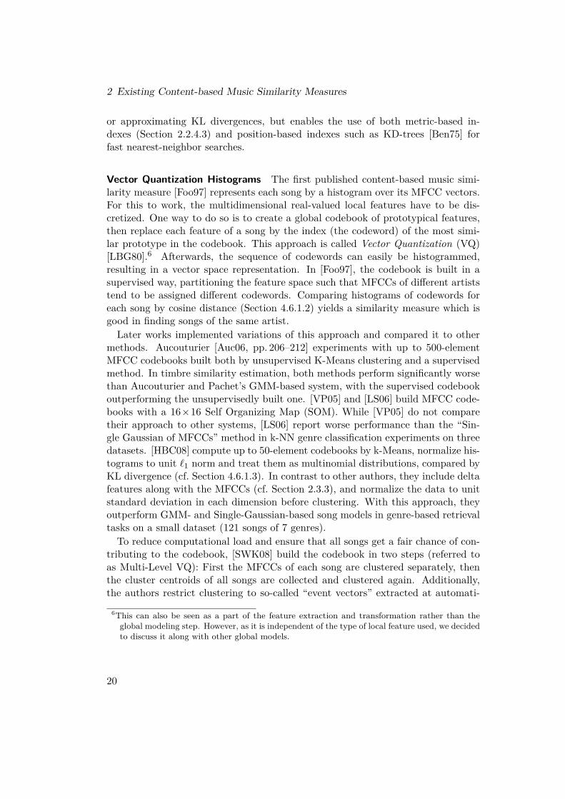
Vector Quantization Histograms The first published content-based music simi-larity measure [Foo97] represents each song by a histogram over its MFCC vectors.For this to work, the multidimensional real-valued local features have to be dis-cretized. One way to do so is to create a global codebook of prototypical features,then replace each feature of a song by the index (the codeword) of the most simi-lar prototype in the codebook. This approach is called Vector Quantization (VQ)[LBG80].6 Afterwards, the sequence of codewords can easily be histogrammed,resulting in a vector space representation. In [Foo97], the codebook is built in asupervised way, partitioning the feature space such that MFCCs of different artiststend to be assigned different codewords. Comparing histograms of codewords foreach song by cosine distance (Section 4.6.1.2) yields a similarity measure which isgood in finding songs of the same artist.Later works implemented variations of this approach and compared it to other

methods. Aucouturier [Auc06, pp. 206–212] experiments with up to 500-elementMFCC codebooks built both by unsupervised K-Means clustering and a supervisedmethod. In timbre similarity estimation, both methods perform significantly worsethan Aucouturier and Pachet’s GMM-based system, with the supervised codebookoutperforming the unsupervisedly built one. [VP05] and [LS06] build MFCC code-books with a 16×16 Self Organizing Map (SOM). While [VP05] do not comparetheir approach to other systems, [LS06] report worse performance than the “Sin-gle Gaussian of MFCCs” method in k-NN genre classification experiments on threedatasets. [HBC08] compute up to 50-element codebooks by k-Means, normalize his-tograms to unit `1 norm and treat them as multinomial distributions, compared byKL divergence (cf. Section 4.6.1.3). In contrast to other authors, they include deltafeatures along with the MFCCs (cf. Section 2.3.3), and normalize the data to unitstandard deviation in each dimension before clustering. With this approach, theyoutperform GMM- and Single-Gaussian-based song models in genre-based retrievaltasks on a small dataset (121 songs of 7 genres).To reduce computational load and ensure that all songs get a fair chance of con-

tributing to the codebook, [SWK08] build the codebook in two steps (referred toas Multi-Level VQ): First the MFCCs of each song are clustered separately, thenthe cluster centroids of all songs are collected and clustered again. Additionally,the authors restrict clustering to so-called “event vectors” extracted at automati-

6This can also be seen as a part of the feature extraction and transformation rather than theglobal modeling step. However, as it is independent of the type of local feature used, we decidedto discuss it along with other global models.

20


cally estimated note onsets. This measure performs similar to the “Single Gaussianof MFCCs” in k-NN genre classification (3180 songs, 19 genres), but produces farfewer hubs. [MLG+11] also build a codebook in two steps, but using GMMs tofind the most significant frames per song and k-Means only for global clustering.MFCCs are combined with a small set of further frame-wise features (Section 2.3.2).For comparison, they also create a codebook by randomly sampling local featurevectors from songs. Interestingly, this random codebook performs best both in sim-ilarity estimation (evaluated via k-NN genre classification) and classification. Like[SWK08], the authors of [MLG+11] observe that histogram-based models producefewer hubs than Gaussian models.

Spectral Histograms Another way to discretize and histogram local features isby binning. [PDW03] calculate a histogram directly on a song’s log-frequency log-magnitude spectrogram, with a fixed quantization of 20 frequency bands and 50loudness levels, accumulated over the song. However, this model performs con-siderably worse than Aucouturier’s GMM [Auc06, p. 206]. [XZ08] use a similarhistogram, quantizing frequencies into 12 semitones and separately accumulatingover 8 subsequences of the songs. They report their model to perform well in coverdetection and genre classification, albeit on much too small datasets to draw anymeaningful conclusion (14 and 12 songs, respectively).

HDP As a variation on the GMM and VQ models, [HBC08] train a HierarchicalDirichlet Process (HDP) on all local features (frame-wise MFCCs plus their deltas)of a database. This can be seen as a GMM with indefinitely many Gaussian com-ponents, of which only a finite subset is used to explain the training data. A songcan then be represented by calculating the posterior distribution over the Gaussianmixture weights given the song’s local features, which yields a representation thatis conceptually similar to a normalized VQ histogram, but defines a Dirichlet dis-tribution rather than a multinomial. Comparing the Dirichlet distributions of twosongs by the KL divergence, the authors obtain a fast similarity measure that out-performs Gaussian-based models and produces fewer hubs (on the small 121-piecegenre-retrieval dataset mentioned above).

Dynamic Modeling In order to include information on the time course of a mu-sic piece rather than completely discarding the order of local features (cf. Sec-tion 2.2.4.2), several authors have tried to employ sequential data models. Mostprominently, Hidden Markov Models (HMMs) with GMM observations have beenused to model sequences of local features. For similarity estimations, these modelscan be compared by the Monte-Carlo approximation of the KL divergence describedabove (Equation 2.6), replacing the unordered sets of samples with sequences. Re-

21


sults, however, have been disappointing: [Auc06, pp. 202–204] see no improvementin timbre similarity estimation over a static GMM. Similarly, in [SZ05], (genre-wide) HMMs perform worse than a static SVM in genre classification, and a typeof recurrent neural networks called Elman networks gives even worse results. Uponcloser examination, [FPW05] find that HMMs actually provide a better song modelthan GMMs in terms of the likelihood, but fail to improve similarity estimations(evaluated via k-NN genre classification). This suggests that HMMs do success-fully model dynamic aspects of the songs, but none of these aspects are relevant fordiscriminating music.In Section 2.3.3, we will discuss approaches to capture temporal aspects directly

at the feature extraction stage instead.

Feature Selection One of the implicit assumptions of all statistical models of localfeatures is that the most statistically significant features are the most important(Section 2.2.4.2). To weaken this assumption, several authors have tried to includeonly a subset of a song’s local features in the global model.7 Both [SWK08] and[Sca08] restrict the global model to local features centered at likely note onsets, asdetermined by an onset detection function. While the main motivation in [SWK08]was to reduce computational costs, [Sca08] hoped to achieve some translation invari-ance. None of the authors compared their method to an implementation withoutonset filter, but [SWK08] noted that their models tended to only model percussion,which possibly degraded similarity estimates of their system. [SPWS09] instead fil-ter out and discard low-energy frames, having found that they contribute much tothe similarity estimate in the “Single Gaussian of MFCCs” approach although thesilent parts of songs are arguably not the most perceptually relevant. By discard-ing between 50% and 70% of the lowest-energy MFCCs, k-NN genre classificationaccuracy improves from about 19% to 22% (on a dataset of 3180 songs and 19genres).

Distance Transformations Some attempts have been made to improve a similar-ity measure by post-processing the calculated distances. [PSS+09] and [SWP10]calculate a full distance matrix between all songs of a collection, then normalizeeach distance with respect to the mean and standard deviation of distances in thecomplete row and column (Distance Space Normalization). This changes the near-est neighbor ranks, often improving k-NN genre classification results [PSS+09, p. 5],[SWP10, Table 1]. Building on this idea, [SFSW11] model the distribution of neigh-bor distances to each song as a Gaussian, then interpret the Gaussian’s cumulative

7Here, “feature selection” refers to filtering the sequence of local features in time, rather thantrying to find a combination of different kinds of features that is suited best for a particulartask.

22


density function as a mapping from distances to negated probabilities of being aclose neighbor. Combining these neighbor probabilities (Mutual Proximity), theyobtain an affinity matrix with more symmetric neighborhood relations, which re-duces the number of hubs and improves k-NN genre classification. See [SFSW11]for references to further approaches.With a different goal in mind, Schnitzer et al. [SFW09, SFW11] explore a way to

map Gaussian-based song models to low-dimensional vectors such that Euclideandistances in the vector space closely resemble the KL divergences of the originalmodels. This allows to use fast indexing methods even for the non-metric Gaussian-based similarity measures.

Metric Learning [SWW08] experiment with four methods to map song modelsto low-dimensional vectors such that their Euclidean distances approximate knownsimilarities between music pieces. Binary similarity ground truth for learning andevaluating the mapping was obtained from song metadata (“same album” or “sameartist”) or by mining the web (“posted in the same music blog”). k-NN classificationresults on separate test data show that their new global models (the low-dimensionalvectors) significantly outperform the original models in classification accuracy.[MEDL09] propose a different way to learn a metric: They train a classifier on

pairs of global models to learn binary similarity ground truth. The global modelsare single Gaussians of MFCCs and autocorrelation coefficients and two song-levelfeatures (all concatenated into a single vector), the classifier is a Multi-Layer Per-ceptron (MLP) pre-trained as a Stacked Denoising Autoencoder (SdA), and thesimilarity ground truth is obtained from playlists of commercial radio stations.The classifier successfully learns to distinguish probable from improbable playlisttransitions, and its predictions can be used as a measure of song similarity.

Semantic Models Some authors report improved results with a semantic modelbuilt on top of a feature-based song model. Such a model can be built by supervis-edly training a tag predictor on song models, e.g., a set of binary classifiers each ofwhich outputs the probability that a human would label a given song with a partic-ular tag. Ground truth is obtained by asking a sufficiently large group of humansto label a collection of songs (either in a controlled experiment, or in public webservices such as last.fm described on p. 2). Each tag usually consists of one or fewdescriptive words, such as “hard rock”, “fast”, or “work out”, and the set of pos-sible tags is restricted either beforehand or afterwards by regarding a limited-sizevocabulary only. The collection of tags for a song carries semantically meaningfuldescriptions in terms of genre, mood, instrumentation, singing or preferred listeningcontexts. The idea of semantic models is to learn how humans describe songs interms of tags, then generate hopefully good descriptions for previously unseen songs

23


based solely on their audio content. The predicted tag probabilities (or tag affini-ties) for a song form a high-dimensional vector which can be used as a higher-levelvector space song model – put differently, the tag predictor maps an audio-basedmodel into a new “tag feature space” in which songs can be compared to eachother. [BCTL07] and [Sey10], to name but two examples, report better similarityestimates with such models, compared to purely feature-based models. However,training the tag predictors requires a large collection of high-quality ground truth.

2.3.2 Short-term Local Features

As an alternative or supplement to MFCCs, a wealth of other short-term featureshas been suggested, each trying to capture a specific aspect of the spectrum on atime scale of one to three frames.

Spectral Shape The spectral centroid, spread, skewness, kurtosis, slope and roll-off give different scalar descriptions of aspects of the spectral envelope, calculatedon each mel-spectral frame (see e.g., [Pee04, Sec. 6], [TC02]). Variations of thespectral flatness [Pee04, Sec. 9] and spectral contrast [JLZ+02, ASH09] measurethe noisiness or tonality of frames by regarding the difference between valleys andpeaks in the spectrum. More music-specific features aim to find the fundamentalfrequency [DR93] or the notes present in a frame (“chroma” features [SGHS08]).

Dynamics Features such as the spectral flux [Pee04, Sec. 6.2] or delta and dou-ble delta (acceleration) features [Fur86] aim to capture some of the dynamics of asignal. While the former is defined directly for spectra, delta features just com-pute the difference of consecutive frame-wise features (and acceleration featurescompute the difference of consecutive deltas) and are applicable to any kind oflocal feature. This simple extension helps a lot in speech recognition [Fur86] andmitigates the exchangeability assumption in Bag-of-Frames models for music (seeSection 2.2.4.2).8

Learned Features As an alternative to such hand-crafted features, some attemptshave been made to learn short-term features, but only in classification tasks.9[HWE09] train a Deep Belief Net (DBN, see Section 4.4.3 on p. 75) on a set ofMFCCs and other short-term spectral features described above, then fine-tune it toclassify frame-wise features into instruments, with comparable results to an SVM

8Actually, frames plus delta frames are a representation of bigrams, and if there are no duplicateframes in a music piece, a set of bigrams already suffices to reconstruct the complete originalsequence.

9So learning could just as well be seen as a part of the classifier, not the feature extraction, butit is still an interesting approach to consider.

24


and MLP classifier. [HE10] instead train a DBN directly on spectral frames (i.e.,the high-dimensional frame-wise DFT result), then extensively fine-tune the net-work as a genre classifier. Removing the DBN’s classification layer, they use thenetwork as a frame-wise feature extractor, and train an RBF-kernel SVM to classifythe features into the genres they have previously been tuned for. Classifying songswith a winner-takes-all scheme, they show that their tuned local features outper-form MFCCs in separating said genres (when mapped to an infinite-dimensionalfeature space by the RBF kernel). However, it is unclear whether these specializedfeatures would be useful for a general genre-independent music similarity measure.

2.3.3 Long-term Local FeaturesSeveral features have been designed to capture more long-term information thanthe frame-wise spectral energy distribution (and its frame-wise deltas).

ZCR One of the most primitive long-term feature is the Zero-Crossing Rate (ZCR).It is calculated directly in the time domain and gives the number of sign changesbetween consecutive samples per time unit (i.e., the number of times the signalcrosses the zero amplitude line). While fast to compute, it is difficult to interpret –it is dependent on the frequency (higher frequencies have a higher ZCR), but canalso be regarded as a measure of noisiness.

Texture Windows Other features build on frame-wise features. For example, asimple way to include more long-term information in local features is to form so-called Texture Windows: Frame-wise features such as MFCCs are aggregated overwindows of one or a few seconds, and each window is represented by simple statis-tics such as the mean and variance of its frame-wise features. These statistics formnew higher-dimensional long-term local features. [Auc06, pp. 201–202] do not findany improvement in their timbre similarity estimates with this approach. However,[TC02] and [WC04] obtain a significant improvement in genre classification accuracywhen compared to directly modeling frame-wise features. As a variation, [WC05]compute statistics over onset-aligned windows rather than fixed-size windows, fur-ther improving results. [SZ05], however, neither see a significant improvement nordegradation with beat-aligned windows.

Block-wise Features A more explicit way to locally model dynamics is by process-ing blocks of consecutive frames, i.e., excerpts of a sequence of short-term features.In contrast to texture windows, the order of short-term features within a window iskept, allowing to infer information about the time envelope of a note, the rhythm,or note transitions. Even a simple concatenation of a couple of short-term fea-tures yields long-term local features that can help in classifying music into genres

25


[SZ05]. More advanced features are obtained from further processing such blocksof short-term features.Using mel-spectral frames as short-term features (i.e., MFCCs without applying

the DCT), blocks of features are equivalent to spectrogram excerpts with log-scaledfrequency and magnitude. Many state-of-the-art features are based on this repre-sentation. Fluctuation Patterns (FPs) [PRM02][Pam06, pp. 36–42] aim to capturerhythmic aspects of a song. Their key idea is to apply an FFT to each frequencyband of 3- to 6-second blocks, thus determining regular modulations of loudnessover time (separately for each frequency band). Only modulations of 0–10Hz areregarded, corresponding to 0–600 beats per minute (bpm). Results are weightedaccording to a perceptual model, attenuating very slow modulations, peaks in thepattern are emphasized with a gradient filter, and the final pattern is smoothed witha Gaussian filter both with respect to modulation frequencies (periodicities) andfrequency bands, to enable a more fuzzy comparison of patterns. [SWP10] scale theperiodicities of fluctuation patterns logarithmically, such that a change in temporesults in a linear shift along the periodicity axis of the patterns. The filter bankused for the rescaling step also induces a loss of precision, such that the patternsbecome invariant to minor changes in tempo. [PSS+09] do the same, but applyan onset filter before computing the modulation strengths (resulting in Onset Pat-terns). The onsets are determined on a high-resolution cent scale rather than theusual coarse mel scale, then reduced to a low-resolution critical band representation,aiming to reliably detect note onsets only semitones apart without increasing thedimensionality of the final pattern. Several higher-level features are derived fromfluctuation patterns: [Pam06, pp. 57–45] suggests to compute the center of grav-ity, the focus (whether modulations are concentrated in a few periodicity-frequencybins or widely spread over the pattern) and various ratios of energy in specificranges of periodicity and frequency. [PSS+09] apply a 2D DCT to the patterns andkeep a limited range of Onset Coefficients in both dimensions. The suitability offluctuation patterns for modeling rhythms has been demonstrated on a dataset ofballroom music, in which they significantly outperformed MFCCs in terms of k-NNgenre classification [PSS+09].[SWP10] propose a range of additional features based on log-frequency log-

magnitude spectrogram excerpts. The Spectral Pattern takes short blocks of 10frames and sorts the 10 time steps of each frequency band by value. The Delta Spec-tral Pattern does the same on 25-frame blocks of a spectrogram with emphasizedonsets (by calculating differences and half-wave rectifying the result). The Corre-lation Pattern measures the correlation between frequencies in 256-frame blocks,and the Spectral Contrast Pattern calculates the frame-wise spectral contrast men-tioned in Section 2.3.2, then sorts the values of each frequency band in blocks of 40frames. The calculations, block lengths and the number of frequency bands havebeen carefully tuned for each of these features.

26


[PKSW10] apply two hand-designed image filters to a cent-scaled spectrogramwhich emphasize horizontal and vertical patterns, respectively, i.e., continuous tonesand short attacks. Calculating the means over the two filtered spectrograms anddividing the “attack” mean by the sum of the two means yields a scalar featuredubbed the H2A ratio. Low values indicate a dominance of harmonic parts, highvalues indicate strong percussion. This can be calculated as a global feature forsorting songs [PKSW10], or on a local level like other features [PSS+09].

Learned Features Like for short-term features, attempts have been made at learn-ing features rather than hand-crafting them. [Abd02] shows that applying Inde-pendent Component Analysis (ICA) to short music waveform excerpts yields com-ponents similar to Fourier basis functions, and that sparse coding of harpsichordmusic spectrograms could reveal notes. [HBC09] train a shift-invariant HDP onspectrograms and yield decompositions of songs into musically meaningful compo-nents such as drum sounds and vocals, as well as transcriptions of songs in terms ofthese components. However, such complex song descriptions are not directly usablefor similarity estimation. Lee et al. [LLPN09] train convolutional DBNs on spec-trograms (compressed on the frequency axis via PCA), yielding 10-frame featuresthat surpass MFCCs in 5-way genre and 4-way artist classification on 3-secondsong snippets (not stating the classification method used). However, it is unclearwhether the features are useful for similarity estimation as well, and it is possiblethey outperform MFCCs simply because they integrate information over multi-ple frames. [PKSW06] apply ICA to PCA-compressed mel-sone music spectrogramexcerpts and compare the components’ activation histograms for music pieces to es-timate their musical similarity. However, in 1-NN genre classification this approachproves inferior to Aucouturier and Pachet’s method. [PBK09] unsupervisedly ex-tract features from a high-dimensional cortical representation of music pieces usingLocality-Preserving Non-negative Tensor Factorization (LPNTF). They then traina supervised sparsity-based classifier on these features and surpass state-of-the-artresults on two genre classification datasets. However, it is unclear if this is becauseof the features or because of the classifier.

2.3.4 Combined Features

State-of-the-art systems combine short-term features with long-term features, yield-ing a similarity measure that regards both timbral and rhythmic aspects. Combin-ing different features has been shown both to improve similarity estimates and toreduce hubness [FSGP10].Pampalk’s G1C [Pam06] combines the “Single Gaussian of MFCCs” with Fluctu-

ation Patterns (and two higher-level features derived from the patterns, the Gravityand Bass). Distances are computed separately with KL divergence and Euclidean

27


distance, respectively, then linearly combined with hand-tuned weights. This mea-sure won the MIREX 2006 music similarity and retrieval task.10

Pohle’s RTBOF11 [Poh10, PSS+09], winner of the MIREX 2009 music similar-ity and retrieval task, augments MFCCs with Spectral Contrast, Harmonicnessand Attackness features, modeled as a full-covariance Gaussian for each song andcompared by the Jensen-Shannon divergence (see Section 4.6.1.4, p. 83). This tim-bre component is combined with onset coefficients, which are modeled as a secondGaussian per song and also compared by Jensen-Shannon divergence. The timbreand rhythm distance matrices for a collection are separately normalized with DSN(Section 2.3.1, p. 19) and added up to form the final distance matrix.Seyerlehner’s BLS (Block-Level Similarity) approach [Sey10, SWP10] separately

computes distance matrices for the Spectral Pattern, Delta Spectral Pattern, Vari-ance Delta Spectral Pattern, Fluctuation Pattern, Correlation Pattern and SpectralContrast Pattern (each aggregated to a global model via different percentiles, thencompared by Manhattan distance), normalizes the distance matrices with DSN,linearly combines them with weights optimized on a genre classification dataset,and renormalizes the final distance matrix again with DSN. On the dataset it hasbeen optimized for, BLS beats RTBOF; on five other datasets it performs similarlyor inferior to RTBOF. Combining BLS with RTBOF (again by applying DSN tothe separate distance matrices, adding them and applying DSN to the result) yieldsa similarity measure surpassing both BLS and RTBOF in k-NN genre classificationon six datasets [SWP10].

2.4 Conclusions

From the preceding discussion of existing content-based music similarity estimationsystems, we can draw several insights useful for building our own system, aimingto compete with the state-of-the-art:

1. First of all, the general architecture of a local feature extraction, global mod-eling and comparison stage is well-tested and does not call for a change.

2. Machine learning has been employed at all stages, but not often for feature ex-traction. In particular, unsupervised learning methods for feature extractionare almost unexplored in the context of music similarity estimation.

10MIREX (Music Information Retrieval Evaluation eXchange) is a yearly contest held in con-junction with the International Society for Music Information Retrieval Conference (ISMIR).The audio similarity and retrieval task evaluates music similarity measures via human listeningtests. See http://www.music-ir.org/mirex/ for more information.

11“Rhythm-Timbre Bag of Frames” (RTBOF) is the name given to it in [SWP10]; Pohle termedit the “unified” algorithm.

28

http://www.music-ir.org/mirex/

2.4 Conclusions

3. Capturing the temporal evolution of music pieces with sophisticated dynamicmodels of local features (HMMs, Recurrent Neural Networks) does not seemto work well. Block-wise local features constitute a much better way formodeling dynamics, significantly surpassing simple frame-wise features.

4. The best-performing methods are based on block-wise features defined as elab-orate transformations of log-frequency log-magnitude spectrogram excerpts.These features have been hand-crafted over the course of several doctoral dis-sertations [Pam06, Poh10, Sey10], sometimes optimized to a specific dataset,and include several elusive design decisions and parameter choices. It wouldbe desirable to find more effective, more efficient or better justifiable features.The prevalent basis of log-frequency log-magnitude spectrogram excerpts maybe a good starting point for this.

5. State-of-the-art systems combine rhythmic and timbral features, which givesbetter results than either type of feature alone. To be competitive, any systemprobably needs to capture both short-term and long-term aspects of songs.

6. Choosing a type of local feature (or a combination of features) and extractingit at a steady rate throughout a song is easy and works reasonably well.Attempts at restricting feature extraction to points of interest in a song, suchas detected note onsets, do not yield a consistent improvement.

7. Vector space song models have a range of advantages over Gaussian-basedmodels: Distances are faster to compute, easier to index (for even fasternearest neighbor retrieval) and less prone to hubs.

We will consider these insights in the design of our system in Chapter 4. Before,we will briefly compare the task of music similarity estimation to similar tasks inother domains that have been explored better, in order to learn about methodsthat could be worthwhile to adopt into our system.

29

3 Inspiration from other Domains ofPattern Recognition and InformationRetrieval

In this chapter, we will take a look at three other fields also dealing with theproblems of extracting features, modeling documents or finding similarities: TextRetrieval, Computer Vision and Speech Processing. We will review some of themethods employed and relate the three domains to the music domain to point outarguments for adopting particular methods, to show how this would be possible,but also to give reasons for why this may fail.1This examination is by no means exhaustive, as it is not intended to form the

central contribution of our thesis. It may be worthwhile to explore the relationsof the domains more in-depth to reveal further methods that could be employedin the context of Music Information Retrieval. Ultimately, however, only empiricalinvestigations can show whether a method works or not.

3.1 Text Retrieval SystemsFirstly, we will regard the field of Text Retrieval. As we will see later, it hasalready inspired several methods for Computer Vision, although at the first glance,text does not seem to have much in common with images. Here, we will introducethe methods in their original context, then reason how to apply them to music.Before, we will briefly describe the purposes of Text Retrieval systems.

Purposes

One of the main areas in Text Retrieval research considers the task of documentretrieval: Given a collection of text documents and a textual query, which docu-ments are relevant to the query? Popular use cases are search engines for a libraryor the world wide web. The query may consist of a couple of words (search terms)entered by a user, or a complete document a user wants to find similar documentsto.

1The strategy of borrowing methods from other domains has been described by Aucouturier as adesign pattern termed “Cross-Fertilisation” [Auc06, pp. 51–52].

31

3 Inspiration from other Domains of Pattern Recognition and Information Retrieval

Another important problem is document classification: Given a document and anumber of classes, which class does the document belong to? Possible use cases arespam detection in emails (classifying emails as “spam” or “ham”) or categorizingscientific articles into topics.

Methods

A big challenge in document retrieval is to make a system fast enough for interactiveuse – consider a web search engine that has to answer requests for the best matchesto a query in a database of up to a trillion documents within seconds. However,here we are mostly interested in how documents can be matched to a query oranother document at all, and how documents can be categorized. Both problemsrequire some abstract model of a document, as simply comparing or categorizingdocuments character by character will not turn up anything useful.The first system for document classification [Mar61] worked as follows: Each

document in a corpus of training items (260 abstracts of scientific articles in in-formatics that had been manually grouped into 32 categories, with each documentassigned to up to 3 categories) was separated into words by trivially splitting thetext at spaces and punctuation. The most frequent logical type words (e.g., “the”,“of”) and nonlogical type words (e.g., “computer”, “data”) of the corpus were re-garded as uninformative and the least frequent words were considered to be tooinefficient to use (as they only occurred in few documents). The remaining wordswere manually reduced to a vocabulary of 90 “clue words” that seemed highly in-dicative of a category. A corpus of test items (145 scientific abstracts manuallygrouped into the same set of 32 categories) was processed by testing each docu-ment for the occurrence of clue words, then computing the posterior probabilitiesthat a document belongs to a particular class Cj , given its clue words W1, . . .Wn.The posterior probability of a class was computed by multiplying the prior proba-bility of the class with the likelihoods of the class under each occurring clue word,using Bayes’ rule: P (Cj |W1, . . .Wn) ∝ P (Cj) · P (W1|Cj) · . . . P (Wn|Cj), where thepriors and likelihoods were estimated from the training data by simple counting.This naively assumes that each word in a document independently contributes tothe probability that the document belongs to a particular class, not regarding theorder or co-occurrence of words in a document; it is consequently termed a NaïveBayes classifier [Lew98]. Despite these simplifications, for 33 of the 66 items thatcontained at least two clue words and were manually assigned to only one category,the predicted category was the correct one.Many of the ideas introduced in [Mar61] are still in use today. Both document

classification and retrieval systems mostly follow the same basic structure: A docu-ment is separated into words, matched against a fixed vocabulary, and representedby a vector denoting the number of occurrences of each vocabulary word in the

32

3.1 Text Retrieval Systems

document. This is commonly referred to as a Bag of Words (BoW) representation,as it disregards the order of words in a document, imaginable as pouring all thewords into a bag. This representation can be used to train a classifier on or fordirectly matching documents against other documents or textual queries.Over time, improvements have been proposed on all levels (see [Seb02] for a

review):

Stemming: Prior to filtering the words with a fixed vocabulary, the words of adocument can be mapped to some nominal form, e.g., from plural to singular,or from conjugated verb forms to infinitive. This stemming removes irrelevantvariations (in a BoW model, grammatical suffixes do not carry any usefulinformation, but only increase the size of the vocabulary).

Term weighting: Instead of binarily distinguishing important from unimportantwords, different term weighting schemes have been proposed [SB88], auto-matically judging the importance of each word of a vocabulary based ontheir occurrence in documents, then weighting words in query matching orclassification. One of the most popular schemes for document retrieval isTF/IDF: The term frequency (TF), i.e., the number of times a word occursin a document in proportion to the document length, is weighted by the in-verse document frequency (IDF), given as the logarithm of the inverse of theproportion of documents in a corpus containing the term. The intuition isthat a word which occurs in almost all the documents is less important (atleast in a discriminative sense) than a word occurring in a small fraction ofthe corpus only.

Topic modeling: The BoW model assumes the occurrences of words in a documentto be statistically independent. However, words are in fact often correlated –for example, the word “milk” will often co-occur with “butter”, but seldomwith “asteroid”.2 More severely, some different words even mean the same(synonymy), such as “buy” and “purchase”. To respect this, Latent SemanticIndexing (LSI) [DDL+90] maps document count vectors (the BoW represen-tation) from the original word space to a lower-dimensional space of implicitmeta-terms, or topics, by a linear transformation learned from a corpus. Themapping is learned in an unsupervised way, just regarding the correlations be-tween words, similar to PCA (more concretely, it performs a Singular ValueDecomposition on the term-document occurrence matrix).More recent methods define and learn a generative model of documents. Prob-abilistic Latent Semantic Indexing (pLSI) [Hof99] models documents as mix-tures of topics (i.e., multinomial distributions), and topics as mixtures of

2Despite when speaking of the “milky way”; see the entry about word sense disambiguation.

33


words. To generate a word of a document, it picks a topic from the document-specific mixture of topics, then picks a word from a topic-specific mixture ofwords. The word mixtures for each topic are shared globally, and can berelated to the word-to-topic mapping of LSI. The topic mixtures for eachdocument are estimated from the data, in conjunction with learning the top-ics. The topic mixtures then serve as compact document representations.While this gives a generative model for all documents of a corpus, it cannotgenerate new documents, because their topic mixture is unknown. LatentDirichlet Allocation (LDA) [BNJ03] solves this by placing a prior on thetopic mixture for documents, which is a Dirichlet (the conjugate prior of amultinomial) chosen to be symmetric (with no preference for any topic) andwith α � 0 (favoring sparse mixtures of topics, i.e., only few active topicsper document). Additionally, a Dirichlet prior is placed on the word mixturefor topics, smoothing the distributions estimated from a training corpus. Inthis model, a new document is generated by picking a topic mixture from theDirichlet, then proceeding as for pLSA. The sparseness enforced by the priorsleads to more useful topics and consequently better document representations.As a further extension, the Hierarchical Dirichlet Process (HDP) [TJBB06]infers the number of topics from the data, instead of requiring the number tobe given in advance.As an alternative to modeling documents as mixtures of topics, Salakhutdi-nov and Hinton [SH09b] model documents with two-layer undirected graph-ical models called Restricted Boltzmann Machines (RBMs, see Section 4.4.1,p. 61). One of the layers models word occurrences in a document with a specialarchitecture termed Replicated Softmax, and the second layer consists of la-tent binary units indicating the topics of the document. The latent units forma Product of Experts [Hin02] which multiply and renormalize their predictionson words. This conjunctive coding produces much sharper probability distri-butions over words than the disjunctive coding of mixture models [HS11], andthe latent representations of documents outperform LDA representations indocument retrieval [SH09b].

Semantic hashing: Extending the idea of modeling documents with RBMs, Salak-hutdinov and Hinton [SH09c, HS11] train a stack of three RBMs on word countvectors to form a deep generative model with a small top layer and fine-tunethe resulting four-layer network as a deep autoencoder (in which the formertop layer forms an information bottleneck). The small layer now producesbinary codes for documents such that similar documents are assigned closecode words (in terms of Hamming distance). Using very short codes (e.g., 20bits), this allows indexing all documents by their code, and quickly retrieving

34

3.1 Text Retrieval Systems

similar documents to a query by simply accessing all codes in a Hamming ballaround the code of the query document, without any search.

Word sense disambiguation: The approaches above assume that each entry in adocument’s word count vector refers to a specific word with a specific meaning.However, if these words are directly extracted from a text by splitting it atword boundaries, this assumption does not hold: In most languages, thereare groups of words called homographs that share the same spelling, but havedifferent meanings. For example, “train” can refer to a vehicle or the actof teaching; “bank” can refer to a credit institution, the side of a river, afilter bank, and more. Word sense disambiguation techniques try to infer themeaning of a word by its context (see [Nav09] for a survey). Without wordsense disambiguation, topic models will always regard the average meaning ofa word – for words with a seldom used second meaning (such as “bass”, whichrefers to low sound frequencies far more often than to a species of fish), thisproduces reasonable results in most instances, but for other words, it maywell reduce performance.

n-gram models: The topic models discussed above model the words of a documentindependently. To incorporate at least the immediate local context, wordscan be modeled in pairs or triplets; more generally, in n-grams (n-tuples ofconsecutive words). [Wal06] extends LDA by a bigram topic model, yieldingbetter generative/predictive performance and better topics, which may beuseful in categorization and retrieval tasks.

AdoptionRegarding songs as documents, the basic architecture of text retrieval systemsshows a clear resemblance to content-based music similarity estimation systems(Section 2.1, p. 9): Documents are split into short entities, which are first processedseparately, then aggregated into a more compact global model (abstracting fromthe order of local entities) for classification or comparison purposes. However, it isnot immediately clear how to reasonably relate music pieces to text documents inorder to apply text retrieval methods to music.Let us consider a very straightforward mapping first: Words, the local entities

of documents, could be assumed to be equivalent to frames, the prevalent segmen-tation of music signals. Stemming may be regarded as the equivalent to vectorquantization of frames (or frame-wise features), which also maps slightly differentvariations of local entities to a common form. However, vector quantization alsoenforces a fixed-size vocabulary – in text retrieval, filtering for a set of “clue words”constitutes a separate step. Creating a BoW model as a word count vector canbe directly adopted to a vector-quantized sequence of audio frames, resulting in a

35


“Bag of Frames” (BoF) model. This equivalence has already been pointed out by[RHG08], who refer to their vector-quantized frame-wise chroma features as “audiowords”.For once accepting this equivalence, we can easily apply text retrieval methods

to songs. N-grams would be equivalent to blocks of frames, which are alreadyused in several music similarity measures. Word sense disambiguation could be amore intelligent way to incorporate context information and eliminate ambiguitiesin the interpretation of single frames. Term weighting can be applied to BoFmodels exactly as for BoW models, possibly solving the problem of distinguishingimportant from unimportant frames. In fact, [Foo97] already suggests to weightvector quantized features by their inverse entropy (which would devaluate featuresthat occur nearly uniformly), and [RHG08] use TF/IDF weighting on their “audiowords”. Topic models could form useful representations of songs, and [HBC08]successfully applied HDPs in a music similarity estimation context, albeit modelingtopics as Gaussian distributions of MFCCs rather than multinomials over discreteword-like features. Semantic hashing may be a suitable way to implement fastsimilarity queries on large databases, but require a large database to train on inthe first place.However, it is doubtful whether audio frames are a proper counterpart to words

in text. In contrast to words, frames are very short and always have the samelength – a “Bag of Frames” may thus be more equivalent to a “Bag of Syllables”than to a “Bag of Words”, and shuffling around syllables in a text would obviouslydestroy most clues about its meaning or topic. Syntactically, words in text canbe found via blanks and punctuation. The equivalent in music may be bar lines,although again this would force all words to be of the same length, and lead toan extraordinarily large vocabulary. Regarding pauses as blanks may be tempting,but pauses are scarce at least in popular music. Semantically, there is no consensuson a definition of words, but “perhaps a word is the smallest unit of language thatcan be used by itself” [BS81]. With this loose definition, words in music could benotes. However, unlike words, notes in music overlap, suggesting the need for sourceseparation to properly divide a song into words (separating critical bands could beseen as a half-hearted attempt at this). Apart from that, single notes arguably donot carry as much information as single words – occurrence of the word “soccer”probably limits the possible topics of a document much more than a c′ played on apiano tells about the genre of a song.All in all, although we pointed out a way to apply text retrieval methods to

music via vector quantization of local features, it is not clear whether this is a goodway and what might be a better one. However, the discussion of computer visionsystems will show that text retrieval methods have been successfully applied toimages in a similar way, encouraging their use on music.

36

3.2 Computer Vision Systems


We will now examine the field of Computer Vision. We will first describe the prob-lems it aims to solve, comparing them to tasks in Music Information Retrieval, thenreview the basic methods it employs, and finally see how these could be adopted.

Purposes

Computer Vision research works on methods for extracting information from im-ages. For our purposes, it suffices to regard two broad categories of problems:

Object recognition: Given an image, which objects are present and where? Thisincludes a whole range of more specific tasks:• Classifying images of single objects (e.g., cars, dogs, airplanes . . . )• Classifying images of scenes (e.g., beach, wood, city . . . )• Character recognition (printed or hand-written)• Multiple object detection (e.g., finding cars, humans or faces in surveil-

lance images or videos)• Face recognition (identification of persons from an image of their face)

Image retrieval: Given a collection of images and a query, which images match thequery?• For a textual query, this requires generating a description of each image

the query can be matched against (this description does not need to betextual, but it needs to be relatable to the query).

• If the query is an image, this involves some sort of comparison of thequery image to the images in the collection.

Object recognition mainly deals with classification problems at different levels ofdifficulty, from a low number of classes (recognizing scenes or digits) to a highnumber (face recognition) and from low intra-class variability (printed characterrecognition) to high variability (object classification). As with any classificationtask, difficulties arise either in capturing the inter-class differences (e.g., distin-guishing cats from dogs, or even different kinds of cats), or in ignoring intra-classvariability (e.g., different lighting conditions and orientations in face recognition).Multiple object detection plays a special role in that the number and position ofobjects is not known beforehand. Image retrieval, on the other hand, could ei-ther build on object recognition or, when querying by image, on image similarityestimation.

37


Relating these problems to Music Information Retrieval and regarding songs asthe equivalent to images (we will scrutinize this equivalence further below), we findthe following:• Scene recognition in images is roughly equivalent to genre classification inmusic: Both deal with documents that have a rich local structure, but canusually be assigned to one of a limited set of global classes. Local structure canbe unspecific (clouds, drums) or highly indicative of a class (trees, distortedguitar). In both problems, classes may be blended (trees on a beach, CountrySoul), and classes can be further divided into sub-classes.

• Multiple object detection is roughly equivalent to music transcription: Bothaim to decompose a complex document into a set of known entities and theirlocations. Both need to be invariant to certain transformations of these enti-ties (lighting conditions, mastering), but extract others (pose, accentuation),and both need to cope with intra-class variability (car shapes, instrumentmanufacturers).

• Image retrieval by images is strongly related to music similarity estimation:As stated above, implementing query-by-image retrieval on an image collec-tion requires a comparison of images, which poses the same problems as acomparison of songs, if we regard images and songs to be equivalent.

MethodsMost methods start by constructing a global model for each image, which is sub-sequently classified or compared against other models. This model should captureaspects relevant to the task, but be invariant to unimportant details (which may in-clude the lighting conditions, scale, or orientation, for example). The global modelcan be built from global image features or by aggregation of local features. Herewe can only give a superficial overview of different features and global descriptors;please see [DJLW08, pp. 17–24] for a more extensive review.Global features include descriptions of shape (determined from an automatic

segmentation of the image), color, or texture, used for scene recognition (the “gist”of a scene [OT06]), single object recognition or texture classification. Local featuresmay either be densely sampled from the image (i.e., on a regular grid) or sparsely,at interest points (e.g., corners). Each local feature describes properties of theimage neighborhood, such as the local image gradient. This description can bemade invariant to rotations (e.g., by normalizing it with respect to the largest localgradient direction) and scale (by computing the properties not only in the originalimage, but also in rescaled versions of it); a popular example being the Scale-invariant feature transform (SIFT) [Low04]. The global model abstracts from theexact locations and values of local features, e.g., by histogramming.

38


An approach especially interesting for us has been inspired by Text Retrieval.[ZRZ02] propose a general framework which regards images as documents composedof keyblocks, in analogy to text composed of keywords. First, small quadraticpatches are extracted from an image on a regular grid, transforming the image intoa 2-dimensional array of possibly overlapping blocks. Optionally a low-level featureis computed for each patch, otherwise the raw pixel data is used. Each patch (i.e.,the feature vector or pixel data) is replaced by the index of the closest keyblockin a dictionary previously obtained by clustering a training set of patches. Theimage can now be regarded as a 2-dimensional array of “visual words”. Differentglobal models can be built from this document-like representation: A histogrammodel states the number of occurrences of each code word, analogous to the “Bagof Words” model in Text Retrieval. The relative term frequency (normalized byimage size) or inverse image frequency (the equivalent of the inverse documentfrequency, see p. 33) can be easily derived from this as well as a boolean modelwhich simply binarizes the term frequencies with a given threshold. To includecontext information, [ZRZ02] also suggest to adopt n-gram models by capturing co-occurrences of different spatial configurations of bi- or tri-blocks. In image retrievalexperiments on three databases, their method outperforms two approaches basedon global color features.Similar architectures are still popular both for image retrieval and classification,

with several improvements:

Dictionary learning and Soft words: Alternatives have been proposed both to ob-taining a dictionary of visual words with k-means, and to computing code-words for local features by hard assignment to the closest keyblock. For exam-ple, [JT05] claim to obtain a more informative dictionary with a radius-basedclustering method, and [vGGVS08] improve performance in scene and objectclassification with soft assignments of features to codewords (via Gaussiankernels). In a recent study, Coates et al. [CN11] decouple dictionary learn-ing from image encoding, evaluating different combinations of clustering andsparse coding methods on three object classification datasets. They concludethat a sparse encoding, i.e., image representations each using only a smallsubset of the dictionary, performs best, almost independently of the chosencodewords.

Pooling: The “Bag of Visual Words” (BoVW) is completely invariant to trans-lations of local features, which may be insufficient to distinguish particularimages from each other (e.g., a blue feature in the top half of an image proba-bly is sky, while in the bottom half it may be a lake instead). As a compromisebetween the global BoVW and the full 2-dimensional array of local features,the global model may be constructed by pooling the local features in a fixedpartitioning of the image, such as a 2×2 grid. Depending on the type of local

39


feature, the pooling operation could be histogramming, computing the mean,minimum or maximum of each section (see [BPL10] for a thorough analysisand references).

Spatial pyramids: To avoid having to find the best pooling resolution for a task,it has been suggested to model images as a Spatial Pyramid [LSP06]: theglobal BoVW histogram is augmented with local histograms at increasinglyfine subdivisions of the image. This technique captures the spatial alignmentof local features with different levels of accuracy, allowing to model, say, aface as a particular arrangement of two eyes, a nose and a mouth rather thana mere collection of these parts, without restricting the positions too much.

Topic modeling: Just like in text retrieval, generative models have shown promis-ing results for image classification. The topic models pLSI and LDA havebeen directly adopted from text retrieval and applied as generative modelsfor BoVW vectors in object and scene classification [SRE+05, FFP05].

Generative image models: Additionally, generative models have also been em-ployed to directly model image pixel data, most prominently methods basedon Restricted Boltzmann Machines (RBMs, see Section 4.4.1, p. 61). RBMsare two-layer neural networks with a visible layer of neurons modeling theinput, and a hidden layer of neurons forming a latent representation. Aftertraining an RBM unsupervisedly on a set of training data, the latent repre-sentation conditioned on an input vector forms a higher-level description ofthe input. A trained RBM can thus be used as a feature extractor. RBMs caneasily be stacked to form a Deep Belief Net (DBN) extracting even higher-levelfeatures (see Section 4.4.3, p. 75).Both RBMs and DBNs have successfully been used to model local imagepatches [Kri09, CLN10] and complete small images (e.g., in digit recognition[HOT06, BLPL07], but also for modeling scaled-down scene images [KH11]),developing feature detectors adapted to the input data. Ranzato et al. re-cently proposed two extensions of RBMs with even better capabilities formodeling natural images: the mcRBM [RH10] and mPoT [RMH10], pro-ducing state-of-the-art results on public object recognition datasets [RH10,RSMH11].As a compromise between modeling local patches and modeling complete im-ages, Convolutional RBMs [DB08, NRM09] employ weight-sharing to modela grid of local patches of an image, then use max-pooling to create a morecompact higher-level image description. With a generative formulation of themax-pooling operation, [LGRN09] learn a hierarchy of feature detectors fromfine-scaled parts to larger-scale objects.

40


Learning invariance: Especially in the context of digit recognition, an easy methodto make a classifier more robust to intra-class variability is to extend the train-ing set with synthetically transformed training images, keeping the originallabels [LBBH98, p. 14]. Transformations may include translations, small ro-tations, elastic deformations or task-specific manipulations such as varyingthe line thickness for hand-written digits.An interesting alternative is to train a model to represent transformationsindependently from the image content [HKW11], allowing classifiers to useinformation on, say, exact locations only when needed. Such models arereferred to as being transformation equivariant.

Semantic hashing: Based on the idea of modeling images with RBMs, [KH11] traina deep DBN on small images and fine-tune it as an autoencoder to producecompact binary codes. These codes can be used as semantic hashes to quicklyretrieve similar images from a large database, just as it has be done for doc-uments (p. 34).

Adoption

Again, the architecture of image retrieval systems we focused on is very similar tocontent-based music similarity estimation systems (Section 2.1, p. 9), if we regardsongs as an equivalent to images: Images are divided into smaller parts (or down-sampled to a small size), which are processed separately and combined into a globalmodel. And again, to apply any of the methods, we need to find a way to relatesongs to images.A straightforward link is that images are 2-dimensional signals, while music pieces

are 1-dimensional signals. General local features could therefore be computed onsignal excerpts, the 1-dimensional equivalent to image patches. However, audiosignals are very different from images: While image signals are spatially smooth(i.e., neighboring pixels correlate), audio signals rapidly vary spatially. Thus, it isdoubtful whether image features apply well to raw audio signals.Alternatively, the 1-dimensional audio signal can be transformed into a 2-di-

mensional signal by calculating a spectrogram via a Short-time Fourier Transform(STFT) – this adds a new dimension (frequency) at the cost of time resolution; theproportion of time to frequency resolution being determined by the frame size. Asaudio signals change frequencies rather slowly, the spectrogram representation isspatially smooth along the time axis, resembling images much better than the rawsignals. Local features can then be computed on spectrogram excerpts, i.e., blocksof consecutive frames. Any feature applicable to image patches can be directlyemployed on spectrogram blocks, and any global image model can be used on theselocal image-like features.

41


Several authors already suggested to treat spectrogram excerpts as image patchesand adopt image processing methods. [DSN01] extract features from spectro-grams with oriented Difference of Gaussian filters at different scales, but do notachieve convincing results on a small three-way genre classification dataset. [Abd02,pp. 114–115] employs sparse coding to short spectrogram excerpts of harpsichordmusic, yielding features that detect onsets of different notes. The author did notperform music retrieval experiments with these features, though. [CEK05] useHaar-like feature extractors inspired from object detection on spectrograms to dis-criminate speech from music, and [PKSW10] applies simple horizontal and verticaledge detectors to spectrograms to measure the amount of harmonic and percussiveelements. As mentioned in Section 2.3.3 (p. 27), [PKSW06] applies ICA to spectro-gram blocks to extract local features, then builds global models by histogrammingthe component activations and compares histograms to estimate music similarity,performing worse than Aucouturier and Pachet’s method (Section 2.2, p. 11). Un-like the other attempts, [YS09] extract blocks that do not cover the full frequencyrange, but are limited in both time and frequency. In a log-frequency spectrogram,this makes features invariant both to time shifts and transposition. The authorsproduce a dictionary of blocks by random sampling from spectrograms of instru-ment sounds, then create representations of unseen spectrograms by computingthe distances between the spectrogram and the dictionary at each valid location,min-pooling the results. With a k-NN classifier, they achieve satisfactory results indistinguishing solo instruments.To the best of our knowledge, neither vector quantization nor generative mod-

els have been applied to spectrogram patches of music, except for a small-scaleclassification experiment with Convolutional Deep Belief Networks ([LLPN09], seeSection 2.3.3, p. 27). Also pooling or spatial pyramids have not been employed,although they could provide a good model: In music, global arrangement shouldbe less important than local arrangement (for two songs to be similar, it will beunimportant whether a guitar solo takes place before a bass solo or the other wayround). While a BoW of large-scale local features might reflect this, possibly somehierarchy would work better.It is not clear whether spectrogram patches form a good base for methods de-

signed for image retrieval, though. While images pixels are locally correlated inall directions, spectrograms are only smooth in time; correlations in frequency areinfluenced by harmonics (also see Section 5.3, p. 92). Moreover, the two dimensionsin a spectrogram have two very different meanings: one denotes time, the otherdenotes frequency. In images, on the other hand, both dimensions are spatial. Asa consequence, flipped, rotated or rescaled images are often still interpretable, pos-sibly not even changing their meaning (such as a picture showing a soccer ball, ora pen on a desk seen from above), while a rotated spectrogram would not resembleany usual sound at all. This can also be seen as an advantage: To model music,

42

3.3 Speech Processing Systems

we do not need to consider rotation- or scaled-invariant features such as SIFT. Athird difference is that many physical objects are opaque, such that overlappingobjects in an image occlude each other, and, ideally, relevant objects occlude thebackground. In spectrograms, overlapping acoustic events add up instead, possiblyrendering many object recognition methods inapplicable to music.

3.3 Speech Processing SystemsFinally, we take a brief look at the field of Speech Processing. Again, we willfirst compare the problems it targets to problems in Music Information Retrieval,describe commonly employed solutions and see what we can learn for our task.

Purposes

Speech processing aims at extracting information from speech signals. We willregard three exemplary problems:

Speech recognition: The main area of research in this field deals with transformingan audio signal of human speech into a textual sequence of words. Often, thetask is simplified by limiting the vocabulary or targetting a specific speaker.

Speaker recognition: Another problem is to identify the speaker by her or his voice,useful for identity verification or monitoring.

Source separation: The Cocktail Party Problem is the problem of separating outa single voice from a recording of many people speaking simultaneously. Thisis an easy task for humans, who can follow a conversation in a crowded room(e.g., at a cocktail party).

The first two problems are classification problems: Speaker recognition identifiesone of a known set of speakers from a speech signal, speech recognition classifiesshort excerpts into phones. The third problem is a source separation problem,aiming to reconstruct the components of a mixed signal.Insights from speaker recognition might be applicable for instrument recognition,

artist identification, or to estimate singing voice similarities, and speech recognitioncould be similar to finding melodies in music (if we relate phones to notes), butboth deal with a single voice recording, which is very different to polyphonic mu-sic. Solving the cocktail party problem could help to separate a polyphonic musicsignal into a set of “solo parts”, enabling the application of methods for analyzingmonophonic music. However, speech of different speakers at a cocktail party isuncorrelated (except that people within a conversation tend not to speak simulta-neously and share a common topic), while simultaneously playing instruments in a

43


song usually respect a common rhythm and their pitches combine into particularharmonies – put differently, when separating and recombining the sources of twococktail parties, it will still sound like a cocktail party, whereas doing the same fortwo music pieces will generally yield something unmusical (or at least not resembleany popular music).

Methods

Speech recognition is based on modeling sequences of local features. Among themost popular local features are MFCCs, which we described in Section 2.2.1 (p. 11).A sequence of local features is then mapped to a probable sequence of words inmultiple stages: Short sequences of features are mapped to phones (the acousticequivalent to phonemes), sequences of phones are mapped to words and sequencesof words are mapped to sentences. These stages influence each other not only ina bottom-up, but also in a top-down manner: A good language model can predictprobable words from the sentence formed so far, which in turn makes it easier topredict the next phone given acoustic features.The prevalent base for these stages are Hidden Markov Models (HMMs). For each

phone, a separate HMM of a few states is trained to model typical short sequencesof local features [JR91]. These phone-specific HMMs can then be concatenatedto form word HMMs, which can again be concatenated to phrase HMMs. TheHMM’s emission probabilities, i.e., the probability distribution over local acousticfeatures given a hidden state within a phone HMM, are often chosen to be diagonal-covariance GMMs. These have to capture the acoustic intra-class variability oflocal features. To reduce this variability, phone-specific HMMs can be formed foreach biphone or triphone instead – as phones sound differently depending on thepreceding and following phones, including this context eliminates a major source ofintra-class variability (at the cost of a much larger number of first stage models).To be tractable, HMMs make a strong simplifying assumption: given a sequence

of hidden states, the observable local features are treated as conditionally indepen-dent. To still include temporal dependencies between local features, the featuresare often augmented with delta and double delta features [Fur86] (simply joining afew consecutive features instead would not help, as the diagonal-covariance GMMscould not model their dependency either). Several alternatives have been suggestedto include longer contexts: [Rob94] replaces the phone-level HMMs with RecurrentNeural Networks (RNNs) accumulating information from all the past features toestimate the probability of each phone. [Her03] designed a higher-level feature ex-tractor called TRAP-TANDEM which derives information from much longer con-texts than MFCCs, after supervised training of its components. [MDH09] traineda DBN on blocks of 11 consecutive MFCCs augmented with delta and double deltacoefficients, fine-tuned it to classify phones and surpassed the previous state-of-the-

44

3.3 Speech Processing Systems

art on a public phone recognition dataset. [JH11] outperform this method with aDBN trained on pooled features extracted by an RBM from raw signal excerpts.[DRMH10] train an mcRBM on blocks of 15 consecutive mel-spectral frames (i.e.,MFCCs before applying the DCT), then train a usual DBN on the mcRBM’s latentrepresentations as a phone classifier (not backpropagating through the mcRBM inthe supervised fine-tuning phase). As mcRBMs explicitly model the individualcovariance structure of each input example, they naturally capture dependenciesbetween frames without the need for delta features. This approach surpasses [JH11],defining the current state-of-the-art in speaker-independent speech recognition.The problem of speaker recognition is related to, but different from speech recog-

nition. On the surface, both deal with classifying speech recordings. However, atleast speaker-independent speech recognition needs to be invariant to differencesbetween speakers, while speaker recognition aims at capturing just those. Curi-ously, many speaker recognition systems still adopt MFCCs as local features, andGMMs as a “Bag of Features” model [Bei11].Source separation is relatively easy if there are at least as many sensors as sound

sources (see [Mit04]). The problem becomes much more challenging if many soundsources are mixed into a stereo or mono recording (underdetermined source sep-aration). The most basic instantiation of the problem (the case of instantaneousmixing) assumes that N source signals S are linearly mixed into M < N channelsX by a mixture matrix A (which defines the mixing coefficients for each recordingchannel): X = AS. The task is to infer A and S from the observed mixtureX. Tosolve it, the space of solutions has to be restricted by making further assumptions,leading to different methods: Independent Component Analysis (ICA) assumes thesources to be independent and non-Gaussian, Sparse Component Analysis (SCA)assumes the sources to be sparse, and Nonnegative Matrix Factorization (NMF)assumes X, A and S to be nonnegative. Which method is to be preferred dependson the data. ICA has been used on raw signals in [LLGS99] to separate three hu-man speakers in stereo recordings. SCA is not suited well for application to signalsin the time domain, because such signals are not sparse. However, it is possibleto preprocess the sources with a linear transformation that results in sparser data,such as a Fourier Transform. Applying SCA to spectrograms, [BZ01] reconstructthe sources from stereo mixes of four voices, five songs or six flutes with some suc-cess (especially for the songs, notable cross-talk remains). NMF is usually appliedto magnitude or power spectrograms, which are nonnegative by definition [SO06].

Adoption

Just as Text Retrieval, Computer Vision and Music Similarity Estimation systems,speech recognition builds on global models of local features. Speaker recognitiondoes not seem to add anything, but source separation could be useful as an inter-

45


mediate step in processing music.Local features used in speech processing can be directly applied to music, as

both fields handle audio data. And in fact, MFCCs have been adopted to mu-sic similarity estimation from the very beginning [Foo97]. [Sca08] also applied avariation of genre-tuned TRAP-TANDEM features to genre classification, outper-forming MFCCs. The prevalent global speech model, the HMM, has also alreadybeen employed for modelling music, without satisfying results (see Section 2.3.1,p. 21). However, it has only been attempted to directly model complete songs –learning and concatenating separate HMMs for some musical equivalent to phonesand words might improve performance. Generative models for local features havenot been adopted for music similarity estimation, though. The mcRBM approachis especially interesting: It applies a particularly powerful generative model fromcomputer vision to audio data, treating spectrogram excerpts as the equivalent toimage patches, and it achieves state-of-the-art results in speech recognition.Several attempts have been made to apply source separation techniques to mu-

sic, adding domain-specific restrictions on the extracted sources to improve perfor-mance: [VK02] assume signals to be harmonic, [Vir07] assumes continuity in time,and [Bur08] incorporates instrument timbre models. Source separation has not beenemployed for music similarity estimation, but an experiment in genre classificationdid not yield significant improvements [LLT05].

3.4 ConclusionsWhile this exploration revealed a lot of methods possibly useful for content-basedmusic similarity estimation, we will restrict this thesis to a single idea and leaveothers open for our future work. In all three domains, unsupervisedly trainedgenerative models show encouraging results. In particular, the recently proposedmean-covariance Restricted Boltzmann Machine (mcRBM) achieves state-of-the-artperformance in object recognition and phone recognition, modeling image patchesor spectrogram excerpts, respectively. Given that it has successfully been usedto model speech, an application of mcRBMs to music seems straightforward andpromising.

46

4 Proposed New Method

Drawing from ideas and methods mentioned in Chapters 2 and 3, we propose asystem for music similarity estimation that is trained on large amounts of unlabeleddata to learn features for describing music excerpts, then uses these features tomodel and compare music pieces. We will first give an overview of the system,highlighting connections to previous chapters, then discuss each stage in detail.

4.1 The Big Picture

Like existing music similarity estimation systems described in Chapter 2, our systemextracts local features from music pieces, aggregates them to global models andcompares these global models to estimate the similarity of songs. Figure 4.1 detailsour system’s computation steps.The local feature extraction stage transforms the audio signal of a music piece

into a mel-frequency log-amplitude spectrogram and extracts short excerpts from it.The same type of spectrogram is also used for computing MFCCs (see Section 2.2.1,p. 11) and thus well-justified, and processing blocks of multiple consecutive frameshas been shown to be an effective way of capturing the temporal evolution of musicsignals, as we learned in Chapter 2. Specifically, these mel-spectral blocks are similarto what Pampalk et al. [PRM02, Pam06], Pohle et al. [PSS+09, Poh10] and Seyer-lehner et al. [SWP10, Sey10] base their hand-crafted features on, and what Pohleet al. [PKSW06] and Abdallah [Abd02] use for unsupervised learning on music byICA.Instead of directly aggregating these low-level local features into a global model,

an abstraction stage priorly creates a higher-level description of each block. Forthis, the blocks are preprocessed, decorrelating and compressing the data, and thentransformed into binary feature vectors by a mean-covariance Restricted BoltzmannMachine (mcRBM) [RH10], optionally followed by one or more layers of Bernoulli-Bernoulli RBMs. Unlike the low-level feature extraction stage, neither prepro-cessing nor the mcRBM’s and RBM’s feature transformations are hand-crafted:Instead, they are previously adapted to their task by unsupervised training on alarge number of mel-spectral blocks extracted from music pieces. This setup forthe feature extraction and abstraction chain closely follows Dahl’s application ofmcRBMs to speech recognition [DRMH10], but uses longer blocks so it is capable

47


segmentation DFT abs mel filterbank log form blocks

Mel-spectral blocks

Song A

whitening compression

local feature extraction

preprocessing

mcRBM

abstraction

mRBM k-Means

Local high-level features

aggregation

histogram Feature histogram A

cos

measure

`2 `1 KL JSSong B Distance A→B. . . Feature histogram B

normalize

Hanning

DBN

Figure 4.1: Block diagram for the proposed music similarity estimation system. El-lipses denote data, blocks denote transformations, tiled blocks representalternatives.

of capturing musical features that are on a much larger time scale than phones,such as rhythms.To assess the benefit of using an mcRBM for feature abstraction over more basic

models, we compare it to a cheap drop-in replacement for unsupervised featurelearning: k-Means clustering. Despite its simplicity, k-Means has lately been shownto outperform both sparse RBMs and mcRBMs on an image classification task[CLN10], making it an interesting benchmark candidate. It has also been appliedto music feature extraction with both positive and negative results, but only in aframe-wise manner (see Section 2.3.1). Here, we apply it to the same blocks themcRBM is trained on.The system then builds a global model from the sequence of high-level local

features extracted from a music piece. Instead of fitting a Gaussian as in [ME05],[Pam06] or [PSS+09], we compute a histogram of features. Like a Gaussian model,this discards the order of features, but it results in a vector space model similar tothe bag-of-words model commonly used for text documents [Lew98], which enablesthe use of any document retrieval techniques such as term weighting schemes, andpermits computationally cheaper distance measures than those used for comparingGaussian distributions.

4.2 Local Feature Extraction

In the first stage, the system extracts short mel-spectral frames from the audiosignal. Both the computation steps and the chosen hyperparameters are adopted

48


from MFCCs and can be justified as in Section 2.2.1 (p. 11). In the following, wewill describe the computation in detail.First, the signal is segmented into a sequence of (possibly overlapping) short

frames. Formally, we obtain the mth frame xm from a signal (s1, s2, . . . , sN ) as

xm =

s((m−1)h+1)s((m−1)h+2)

...s((m−1)h+l)

, m ∈ [1,M ], M =⌊N − lh

⌋+ 1,

where l and h are the frame length and hop size in samples, respectively. In theMIR literature, MFCCs have been reported to be calculated on frames as short as20ms [RMT+10] and as long as 100ms [MEDL09], typically with 50% overlap. Forour system, we chose a frame length of 64ms and a frame hop size of 32ms, whichfalls into that range, but has not been optimized in our experiments.1Each frame is multiplied with a Hanning window and mapped to the frequency

domain using a Discrete Fourier Transform, yieldingym = D diag(w)xm,

where w is the Hanning window given as

wi = 0.5(

1− cos(2π(i− 1))l − 1

), i ∈ [1, l]

and D is the l-point DFT given as

Dij = e−2π√−1(i−1)(j−1)

l , i, j ∈ [1, l].The phases of these spectral frames are discarded by taking the absolute values,

the frequency bins are multiplied with a mel filter bank to mimic humans’ cochlearpitch perception, and the log function is applied to the resulting filter activationsto imitate humans’ perception of loudness. Formally, we have

zm = log(M |ym|),where log(·) and |·| denote the element-wise logarithm and absolute, respectively.The mel filter bank M is a collection of triangular filters given as

Mij =

0 if f(j) < p(i− 1)f(j)−p(i−1)p(i)−p(i−1) · 1

2(p(i+1)−p(i−1)) if p(i− 1) ≤ f(j) < p(i)f(j)−p(i+1)p(i)−p(i+1) · 1

2(p(i+1)−p(i−1)) if p(i) ≤ f(j) < p(i+ 1)0 if p(i+ 1) ≤ f(j)

, i ∈ [1, d], j ∈ [1, l],

1We chose it such that frames were comprised of exactly 1024 samples in our first experiments,because frame lengths of powers of two allow computing the DFT via the Fast Fourier Trans-form. In these experiments we worked with music sampled at 16 kHz, hence a frame length of64ms. For later experiments, we kept this length of 64ms independently of the sample rate.

49


where f(j) = (j−1)r2(l−1) is the frequency of the jth DFT bin at a sampling rate of r in

Hz, d � l is the number of mel filters, and p(i − 1), p(i), p(i + 1) are the lowest,peak, and highest frequency of the ith mel filter in Hz, respectively. Adjacent filtersoverlap such that each filter’s peak coincides with the next filter’s lower and theprevious filter’s upper limit, and each filter is scaled to unity energy (see Figure 4.2).The filters are spaced linearly on the mel scale such that the lower limit of the firstfilter equals a given frequency p(0) = fmin, and the upper limit of the dth filterequals p(d + 1) = fmax. Computing the remaining peak frequencies is done bymapping p(0) and p(d+ 1) to the mel scale as

P (i) = 1127 log(

1 + p(i)700

), i ∈ {0, d+ 1},

regularly spacing the other peaks on the mel scale as

P (i) = i

d+ 1(P (d+ 1)− P (0)

), i ∈ [1, d],

then mapping them back to Hertz frequencies as

p(i) = 700(eP (i)1127 − 1

), i ∈ [1, d].

We use two different mel filter banks in our experiments: d = 40 log-spacedtriangular filters from fmin = 130Hz to fmax = 6854Hz, and 70 filters from 50to 6854Hz (both depicted in Figure 4.2). The first corresponds to the defaultsetting of yaafe [MEF+10], an audio feature extraction software targetted at musicinformation retrieval, the latter has been manually tuned in an informal listeningtest to provide a clear reconstruction of a short music excerpt featuring drumsand an acoustic guitar, by increasing the frequency resolution and including deeperbass frequencies. We did not increase the upper frequency limit because at leastfor MFCCs, this may make the features sensitive to MP3 compression [SPLS06].The sequence of mel-spectral frames (zm) is then transformed into a sequence of

overlapping blocks (bo) by joining fixed numbers of consecutive frames, similarly tohow we initially formed frames from a sequence of samples:

bo =[z((o−1)H+1) z((o−1)H+2) · · · z((o−1)H+L)

], o ∈ [1, O], O =

⌊M − LH

⌋+1,

where L and H are the block length and hop size in frames, respectively. [DRMH10]used a block length of 15 frames (a hop size does not apply to their setting), but astheir system was targetted at speech recognition, this choice is not necessarily suitedwell for our task. In our experiments, in addition to a block length of 15 frames, wethus tried larger lengths of 39 and 75 frames to enable the system to capture long-term musical features. While 75 frames (corresponding to about 2.5 s of audio) are

50


0 1000 2000 3000 4000 5000 6000 7000frequency / Hz

0.000

0.005

0.010

0.015

0.020

0.025

gain

(a) Default mel bank

0 1000 2000 3000 4000 5000 6000 7000frequency / Hz

0.000

0.005

0.010

0.015

0.020

0.025

0.030

0.035

0.040

gain

(b) High-resolution mel bank

Figure 4.2: Two alternative mel filter banks we use for mapping the linear-frequencymagnitude spectra onto a mel-frequency scale. Each triangular filtercorresponds to a single mel band. The filters are equidistant on the melscale, resulting in log-spaced peak frequencies, and are each scaled toan energy of unity. The second filter bank obtains a higher frequencyresolution and captures deeper bass frequencies.

still shorter than what is used for hand-crafted rhythmic features (e.g., fluctuationpatterns [PRM02] are computed on excerpts of 6 s), our computational resourceswere insufficient for easily processing larger blocks. Additionally, we experimentedwith shorter blocks of 9 frames, which were the shortest blocks yielding interestingfeatures. We set the hop size to the smallest possible value of 1 frame to preventany aliasing effects (cf. [CLN10, p. 7]). We did not try larger hop sizes as we do notexpect a positive effect on the similarity estimation quality, only on computationalefficiency, which is merely a secondary goal.In summary, we obtain themth mel-spectral frame zm from a signal (s1, s2, . . . , sN )

as

zm = log(M∣∣∣D diag(w)

s((m−1)h+1)s((m−1)h+2)

...s((m−1)h+l)

∣∣∣),

then form mel-spectral blocks bo as

bo =[z((o−1)H+1) z((o−1)H+2) · · · z((o−1)H+L)

].

As depicted in Figure 4.3, this can also be interpreted as computing a mel-scaledspectrogram and extracting patches at different positions in time, drawing an anal-ogy to feature extraction schemes from the field of Computer Vision. Note that the

51

20000 40000 60000 80000 100000sample

1.0

0.5

0.0

0.5

1.0

ampl

itude

(a) Sampled audio signal (sn)

1 50 100 150 200frame

5001000150020002500

pitc

h / m

el

(c) Mel-scaled spectrogram

↓

1 50 100 150 200frame

5001000150020002500

pitc

h / m

el

(d) Mel-scaled log spectrogram (zm)

↓

b1

b2

b3

b184

b185

b186

...

(e) Mel-spectral blocks (bo)

→

←

1 50 100 150 200frame

0

1000

2000

3000

4000

5000

6000

7000

8000

freq

uenc

y / H

z

(b) Spectrogram (ym)

Figure 4.3: The local feature extraction process interpreted as computing a spec-trogram, mapping it to the mel scale and extracting patches. The audiosignal (a), here a 6-seconds guitar solo accompanied by bass and drums,is transformed to a spectrogram (b). The guitar solo becomes visibleas two dim curves, the bass as horizontal stripes at the bottom, andpercussion as regularly spaced vertical stripes. Using the mel filterbankof Figure 4.2a, frequencies are mapped to mel pitches (c). Note thatthe harmonics of the guitar are now spaced uniformly, as the mel scaleis logarithmic in frequency, and that frequencies below 130Hz are notincluded. Applying a log function yields the mel-scaled log spectro-gram (d), which emphasizes fine low-volume structures. At each validposition, a mel-spectral block is cut out of this spectrogram (e).

4.3 Preprocessing

computation steps for zm are the same steps as performed in computing MFCCs(see Section 2.2.1, p. 11), just omitting the final Discrete Cosine Transform. As wewill decorrelate blocks of consecutive frames anyway, an invertible linear transformsuch as the DCT would not have any effect at this point. Computing the frame-wise DCT and dropping the highest components, as is commonly done for MFCCsas an approximation to PCA compression, would be similarly unhelpful as we arecompressing blocks of frames later.2

4.3 PreprocessingThe mel-spectral blocks described in the previous section are highly correlated: Inaddition to correlations inherent in music, the overlapping of mel-spectral framesinduces correlations in time, and the overlapping of triangular filters in the mel filterbank induces correlations in frequency. While mcRBMs can deal with correlateddata, training converges faster on whitened inputs [RKH10], and whitening also sig-nificantly improves results with k-Means features (as we will see in Section 5.4.3.3;also cf. [CLN10]).Apart from that, the blocks are high-dimensional, with up to 2730 (39 frames of

70 mel bands) and 3000 (75 frames of 40 mel bands) dimensions. Given the highcorrelation between feature dimensions, we can compress the mel-spectral blocksto lower-dimensional vectors without losing much information, thus reducing thecomputational effort for the feature abstraction stage.Both whitening and compression can be accomplished with computationally

cheap linear transformations learned from the data. In particular, we experimentedwith the PCA and ZCA transformations, which we will motivate and describe inthe following.

4.3.1 WhiteningWhitened data is decorrelated and has zero mean and unit variance in each dimen-sion, so the covariance matrix is the identity matrix. Any data can be whitened,or sphered, by an affine transformation adapted to the data.Assume we have extracted a set of t mel-spectral blocks from music pieces we

use as training data. We reshape each block into an Ld-dimensional row vector(L denotes the block length, d the number of mel bands) and stack these vectorsinto a t × Ld-dimensional matrix X of training data. We will now find an affinetransformation for whitening the training data, which we can subsequently applyto any similarly distributed data.

2Actually, compressing the frames by DCT in this way before compressing the blocks would evenlead to a suboptimal compression scheme in terms of the mean squared error (MSE) of thereconstruction, because the DCT is only an approximation of the optimal PCA transform.

53


To mean-center the data, we simply subtract the population mean:

Y = X − X̄, where X̄ij = 1t

t∑n=1

Xnj

Additionally, we need to rotate and scale the mean-centered training data Y suchthat the transformed data Z has a covariance matrix equal to the identity matrix:

1t− 1Z

TZ = I

Expressing the transformation as a matrix multiplicationZ = YW ,

we thus need to find a matrix W such that1

t− 1WTY TYW = I

WW TY TYW = (t− 1)WWW TY TY = (t− 1)I

WW T = (t− 1)(Y TY )−1. (4.1)Many such whitening matrices are possible. By imposing additional constraints onW , we can derive different whitening transforms holding special properties [BS97].

4.3.1.1 Principal Component Analysis

If we restrict the columns of W to be orthogonal, that isWW T = diag(s) (4.2)

for some Ld-dimensional vector s, the solution is obtained from the eigendecompo-sition of the covariance matrix of the training data: Being real and symmetric, thecovariance matrix can be decomposed as

1t− 1Y

TY = E diag(λ)ET , (4.3)

where the columns of E form an orthonormal set of eigenvectors and λ is the vectorof corresponding eigenvalues. Substituting (4.3) into (4.1), we can solve for W :

WW T =(E diag(λ)ET

)−1

WW T = E diag(λ)−1ET (4.4)

WW T = E(diag(λ)−

12 diag(λ)−

12 T)ET

WW T =(E diag(λ)−

12) (E diag(λ)−

12)T

W = E diag(λ)−12 . (4.5)

54

4.3 Preprocessing

Using the orthogonality of E we can verify that W fulfills (4.2) with s = λ. Notethat computing diag(λ)− 1

2 just requires to separately take each element of λ to thepower of −1

2 .This solution is related to the Principal Component Analysis (PCA): It rotates the

(mean-centered) input data to the space of its principal components, decorrelatingit, then divides each component by the square root of its variance, whitening thedata. To understand the latter, note that the variance of the data Y projectedonto a column e:j of E is directly given by the corresponding eigenvalue λj in λ,as we can infer from the eigenvalue equation by using eT

:je:j = 1:( 1t− 1Y

TY

)e:j = λje:j

1t− 1

(eT

:jYTY e:j

)= λje

T:je:j = λj .

4.3.1.2 Zero-phase Component Analysis

Constraining W to be symmetric, that is

W = W T

WW T = W 2, (4.6)

we obtain a different solution. Substituting (4.6) into (4.4) and solving for W , weget

W 2 = E diag(λ)−1ET

W =(E diag(λ)−1ET

) 12

W = E diag(λ)−12ET . (4.7)

This whitening matrix can be interpreted as rotating the (mean-centered) inputdata to the space of its principal components, dividing each component by itsstandard deviation, then rotating the data back to its original space [Kri09]. It isknown as the Zero-phase Component Analysis [BS97], and we will shortly see why.

4.3.1.3 Discussion

PCA is a well-known data preprocessing step used in many fields of computing. Ithas been chosen as a preprocessor for mean-covariance RBMs [RH10, DRMH10]and has been shown to strongly relate to k-Means clustering [DH04]. ZCA, on theother hand, has recently become popular for decorrelating image patches especiallyin unsupervised settings similar to ours: ZCA whitened image data has successfully

55


been fed to Restricted Boltzmann Machines [CLN10], Deep Belief Nets [Kri09],covariance RBMs [RKH10], Sparse Autoencoders [CN11] and k-Means based vectorquantizers [CLN10, CN11]. Literature does not indicate which of the two methodsis suited better for our problem, so to make an informed decision on the whiteningmethod to use in our setup, we will set PCA in contrast to ZCA, analyzing theircommon properties and their differences.Let us first consider the two-dimensional case to get a better understanding of

the transformations employed by PCA and ZCA. Figure 4.4a shows a set of two-dimensional correlated Gaussian3 observations X. By subtracting the mean, weremove first-order statistics from the data, obtaining the set of mean-centered ob-servations Y (Figure 4.4b). Note that any rotated, scaled or reflected set AYremains mean-centered. From the eigendecomposition of the covariance matrix weobtain the two principal components of Y , shown as arrows. Each arrow is scaledby the standard deviation of the data in direction of the principal component, i.e.,by the square root of the respective eigenvalue. Principal Component Analysisrotates the data such that the principal components become aligned with the co-ordinate axes, which decorrelates the data. PCA whitening additionally scales thedata to unit variance, sphering it (Figure 4.4c). Note that any further rotationor reflection of the data (i.e., multiplication by an orthogonal matrix E) retainsthis spheric property. ZCA employs the specific rotation which reverses the initialrotation of PCA, returning the data to its original orientation (Figure 4.4d). Alter-natively, ZCA can be thought of sphering the data by scaling it along its principalcomponents, without rotating it at all.As was already evident from the formulae, the two transformations are equivalent

except for a rotation of the sphered data. However, we can make two interestingobservations:

1. The unwhitened data (Figure 4.4b) has a principal component of high vari-ance (white arrow) and another one of lower variance (gray arrow). Afterwhitening, these components become indistinguishable using only second-order statistics (as perfectly illustrated by our Gaussian example, which doesnot have any higher-order statistical moments, resulting in Figures 4.4c and4.4d looking virtually the same safe for the gray tones). With PCA whiten-ing, however, they can be trivially distinguished in the new coordinate system,which may facilitate learning in case the principal components capture rele-vant structure in the data. Additionally, this will prove useful for compression.

2. The ZCA transform keeps the orientation of the data unchanged: If dimensionx denoted the value of the first pixel of a gray-tone image, it will still be

3Gaussian distributions are of course a special case, as any whitening transformation resultsin the multivariate standard normal distribution, but it illustrates two key insights withoutdistracting by the shape of the distribution.

56

4.3 Preprocessing

3 2 1 0 1 2 3x

3

2

1

0

1

2

3

y

(a) Original observations

3 2 1 0 1 2 3x

3

2

1

0

1

2

3

y

(b) Mean-centered observations

3 2 1 0 1 2 3x

3

2

1

0

1

2

3

y

(c) PCA whitened observations

3 2 1 0 1 2 3x

3

2

1

0

1

2

3

y

(d) ZCA whitened observations

Figure 4.4: Scatter plots contrasting PCA to ZCA whitening. The observations(a), here a set of 2-dimensional data points (shades of gray merely serveas visual cues), are mean-centered (b) and the principal components,denoted by arrows scaled by the standard deviation of the data in therespective direction, are estimated from the samples. Both transfor-mations scale the data to unit variance in direction of the principalcomponents, thereby sphering it. PCA (c) rotates the data to alignthe principal components with the coordinate axes, allowing to com-press data by projection onto a subset of the axes. ZCA (d) keeps theorientation, allowing to interpret each dimension as before.

57


w :1

-/+ 0.001

w :2

-/+ 0.006

w :14

-/+ 0.050

w :15

-/+ 0.034

w :414

-/+ 0.547

w :415

-/+ 0.527

(a) PCA whitening filters

w :1

-/+ 2.850

w :2

-/+ 0.785

w :14

-/+ 0.424

w :15

-/+ 0.286

w :414

-/+ 0.029

w :415

-/+ 0.028

(b) PCA dewhitening filtersb1W b21W b41W b61W b81W

(c) PCA whitened blocks

w :1 w :2 w :14 w :15 w :414 w :415

0.5 0.0 0.5 1.0 1.5 2.0 2.5 3.0

(d) ZCA whitening filters

v :1 v :2 v :14 v :15 v :414 v :415

0.1 0.2 0.3 0.4 0.5 0.6 0.7 0.8 0.9

(e) ZCA dewhitening filtersb1W b21W b41W b61W b81W

(f) ZCA whitened blocks

Figure 4.5: PCA and ZCA whitening filters and dewhitening filters (or bases) formel-spectral blocks, as well as whitened data (cf. Figure 4.3e).

associated with this particular pixel after the whitening step. Not changingthe interpretation of dimensions could be useful in case of heterogeneous datasuch as multimodal signals. As we will see in the following, it also manifestsitself in the transformation matrices.

Having formed a basic understanding of the two transformations, let us now seehow they apply to our task of decorrelating mel-spectral blocks. Recalling that thetransformed data is computed as Z = YW , the columns of W can be regardedas a set of filters applied to the data, in which the activation of a single filter w:jfor a data point yi: is given by their dot product yi:w:j . Reshaping the filters tod×L-dimensional matrices allows us to directly visualize their effect on mel-spectralblocks.Figure 4.5 visualizes a subset of the filters learned from a million blocks extracted

from music signals. We can immediately see a striking difference between PCA andZCA whitening: The former yields global filters, the latter yields localized filters ofonly small support. This matches our second observation above: ZCA whiteningkeeps each spectrogram bin at its position, decorrelating it from the other bins,while PCA transforms the data to a very different coordinate system. The PCAdewhitening filters (Figure 4.5b) are just scaled versions of the whitening filters (dueto the constraint on the columns of W being orthogonal); the ZCA dewhiteningfilters (Figure 4.5e) reintroduce the correlations removed by the whitening filters.Note how they spread widely both horizontally and vertically, indicating strongcorrelations in time and frequency, and note the horizontal artifacts especially in

58

4.3 Preprocessing

the last two filters shown, resembling harmonics – both is not found in ZCA filterslearned on natural images, cf. [BS97, Kri09]. Another interesting observation is thatthe ZCA filters are almost symmetrical4 and almost convolutional, which could beutilized for computational optimizations. This symmetricity of the filters lead tothe name Zero-phase Component Analysis (considering the spectrum of the filters).Looking at the whitened data, however, seems to counter our insights: Neither

the PCA nor the ZCA whitened data (Figures 4.5c and 4.5f, respectively) resemblethe original inputs (Figure 4.3d). While this was expected for PCA, it needs furtherexplanation for ZCA. As the whitening step scales each principal component to unitvariance, components of small eigenvalues are strongly amplified, and due to thenature of the input data, these components have a high spatial frequency such asthe last two filters in Figure 4.5a (compare their scaling to the other filters shown).Furthermore, the filters remove horizontal and vertical correlations. As a result,the visible structure in the spectrogram, such as the guitar and percussion, becomesinvisible, while fine structures are magnified and look like noise. This would nothappen for smoother input such as the linear-magnitude spectrogram (Figure 4.3c)or most natural images [Kri09].In summary, our investigation does not uncover a clear advantage of one of the

methods over the other. On the contrary: As the only difference is a rotation ofthe data, at least for k-Means both methods will yield the same results (becausek-Means is invariant to orthogonal transformations [DH04, p. 5]). For other featureabstractors, we will try both PCA and ZCA in our experiments. Nevertheless, theinsights of this analysis will prove useful in the following section.

4.3.2 Compression

In addition to decorrelating and whitening the data, we want to reduce the dimen-sionality of the data especially for mel-spectral blocks of high frequency resolutionor many frames. The obvious way to compress data is by redundancy reduction,another one is by removing irrelevant information (we include lossy compressionin this discussion). As correlations are indicating (linear) redundancies, analyzingcorrelations in the data is a possible first step to compressing it, and we alreadydo this for whitening the data. In fact, we can combine whitening and compressioninto a single step.Examining Figure 4.4b again, Principal Component Analysis finds the direction

of highest variance in the data, and the orthogonal direction. Imagine the specialcase of a dataset having zero variance in the latter direction: the dataset would lieon a one-dimensional linear manifold embedded in a two-dimensional space, and

4Note that this is not implied by the symmetricity constraint on W – the constraint means thatthe first filter determines the first component (here, the bottom left pixel) of all other filters,but it still allows individual filters to be asymmetric.

59


could be losslessly compressed to one dimension by projection onto the directionof highest variance (i.e., by regarding only the x coordinates of the samples in Fig-ure 4.4c, as all y coordinates would be zero). If a dataset does not have componentsof zero variance, but variances close to zero, we can imagine that we would not losemuch information by discarding these components – and in fact, applying PCA to adataset and dropping the components of lowest eigenvalues yields a linear transfor-mation to a lower-dimensional space which is optimal in terms of the mean squarederror of the reconstruction [Pea01]. Formally, for a given target dimensionality m,a minimum solution to

1t

t∑i=1‖yi: − (yi:U)UT ‖2,

where t is the size of the training dataset and yi: is the ith mean-centered trainingdata point, is obtained by setting U to the transformation matrix formed from thecolumns of the PCA whitening matrix that correspond to them largest eigenvalues.However, the components of lowest variance are not necessarily irrelevant, that is,

the reconstruction error may not always be a meaningful measure for the informa-tion lost in compressing the data. To better understand what kind of informationwould be lost in our case, let us examine Figure 4.5 again. We sorted the filtersin order of decreasing eigenvalues, so performing PCA compression in addition towhitening would be accomplished by simply discarding output dimensions startingwith the top right pixel in Figure 4.5c. As the corresponding filters have a highspatial frequency (similar to the two rightmost filters of Figure 4.5a), such a com-pressing scheme would be similar to applying a low-pass filter to the data. Thisis often regarded as a form of noise filtering, which is, however, only true for datain which noise is associated with high frequencies. In our experiments we will seewhether it helps or hurts the performance of our music similarity measure.Accepting the reconstruction error as a measure of information loss, the number

of dimensions to discard can be chosen by defining the acceptable error. This canbe trivially accomplished by setting a threshold on the discarded variance, givenby the sum of eigenvalues of dropped principal components. In fact, this is exactlyequal to the reconstruction error [Bis06, p. 565]:

1t

t∑i=1‖yi: − (yi:U)UT ‖2 =

L·d∑i=m+1

λi,

where L · d is the dimension of the mel-spectral blocks, and λ is the vector ofeigenvalues in decreasing order. In our experiments, we will set the threshold inrelation to the total variance of the input data, a common setting being to retain99% of the original variance.Note that this method of compressing the data only applies to PCA whitening.

While we can also drop principal components (columns of E) in the construction

60

4.4 Feature Abstraction

of the ZCA whitening transform, this would only project the data onto a lower-dimensional linear manifold embedded in the original feature space. For exper-iments on high-dimensional mel-spectral blocks we will thus restrict ourselves toPCA whitening, additionally using ZCA whitening as a comparative method onlywhen no dimensionality reduction is needed.


The core of our system is a data-driven feature abstraction stage obtaining usefulhigh-level descriptions of local features. In particular, we train a mean-covarianceRestricted Boltzmann machine (mcRBM) unsupervisedly as a generative model ona large unlabeled training set of mel-spectral blocks, then use its latent representa-tions as high-level features describing any input data.As mcRBMs are a sophisticated type of Restricted Boltzmann Machines (RBMs),

we will introduce the basic binary RBM before proceeding to mcRBMs. RBMs canalso be trained on the latent representations of another RBM, further abstractingthe features. The resulting stack of RBMs forms a Deep Belief Net (DBN), whichwe will briefly describe as well. For all these models we will present their basic idea,explain the maths (with derivations for the binary RBM in the Appendix) and giveseveral intuitions on how and why they work.In addition, we experimented with k-Means clustering as an alternative way of

generating feature descriptions in an unsupervised manner. We used an algorithmthat proceeds data in mini-batches to allow clustering large datasets, and combinedit with a seeding technique known as k-means++, both of which will be describedat the end of this section.

4.4.1 Restricted Boltzmann Machines (RBMs)

4.4.1.1 Basics

A Restricted Boltzmann Machine (RBM) [Smo86] is an undirected graphical model(or Markov Random Field) of two types of units: visible units representing observ-

W weightmatrix

visible units

hidden unitsh

v

Figure 4.6: A Restricted Boltzmann Machine (RBM)

61


able data, and hidden units representing latent variables. The model is restrictedto a bipartite graph such that the visible units form a layer that is fully connectedto a layer of hidden units, with no intra-layer connections (Figure 4.6).An RBM specifies a joint probability density p(v,h|θ) of visible and hidden unit

states v and h, where θ denotes the model parameters (such as the matrix ofconnection weights between units, W ).5 It is an energy-based model [LCH+06]that expresses the probability density in terms of an energy function E(v,h,θ) asa Boltzmann distribution

p(v,h|θ) = e−E(v,h,θ)

Z(θ) , (4.8)

whereZ(θ) =

∑u,g

e−E(u,g,θ) (4.9)

is the normalizing partition function.6Training an RBMmeans finding parameters θ such that the marginal distribution

of the visibles, defined by p(v|θ), approximates the observed distribution of trainingdata, which is equivalent to maximizing the likelihood of the model under thetraining data. Training is unsupervised, that is, it requires only a set of unlabeleddata points to learn from.Once an RBM is trained, the states of the hidden units conditioned on a data

vector, distributed according to p(h|v,θ), can be interpreted as features extractedfrom the data. As there are no intra-layer connections in the model, the hiddenunits are conditionally independent given a data vector, so their states can beinferred efficiently and in parallel. This is beneficial when using an RBM as afeature extractor.Different types of RBMs can be defined by choosing the energy function appro-

priately. In this section, we will only consider the most basic type of RBMs, whichhas binary (Bernoulli-distributed) visible and hidden units (when conditioned onthe respective opposite layer of units). We will first take a deeper look at themathematics, then give different interpretations for what the model represents andhow it is trained. More advanced types of RBMs, including the mean-covarianceRestricted Boltzmann Machine, will be introduced in Section 4.4.2.

4.4.1.2 Mathematics

We will now give a more detailed presentation of the mathematics behind RestrictedBoltzmann Machines. Most of this thesis can be understood from the higher-

5Depending on the type of RBM, v and h can be samples of continuous or discrete randomvariables, so p(v,h|θ) may be a probability density function or a probability mass function. Tosimplify the description, we will use the term “density” throughout.

6In the continuous case, sums over configurations u or g become integrals.

62


level intuitions in Section 4.4.1.3, but for technical details an understanding of themathematical background is required.

Model The most basic type of RBMs is guided by the following energy function:Eb(v,h,θ) = −

∑i,j

viWijhj −∑

i

viai −∑

j

hjbj

= −vTWh− vTa− hTb, (4.10)where the model parameters θ = (W ,a, b) comprise the connection weights, visibleand hidden bias terms, respectively, and v and h are binary states of the visibleand hidden units.The energy function induces a probability density p(v,h|θ) over joint configura-

tions of v and h according to Equation 4.8. From this density we can derive severalother densities discussed in the following.The marginal probability density of the visibles,

p(v|θ) =∑

g

p(v, g|θ) =∑

g e−E(v,g,θ)

Z(θ) , (4.11)

is the density of observable data as estimated by the model; i.e., it defines thedistribution to sample from if using the RBM as a generative model.Alternatively, the generative model may be defined via an implicit prior over

the hiddens and the conditional probability of the visibles given the hiddens (seeSection 4.4.3). The implicit prior is the marginal density of the hiddens:

p(h|θ) =∑

u

p(u,h|θ) =∑

u e−E(u,h,θ)

Z(θ) (4.12)

The conditional probabilities depend on the chosen energy function. For thefunction defined in Equation 4.10, we obtain the following probability distributions(see Appendix A for the derivation):

P (hk = 1|v,θ) = σ(bk +

∑i

viWik

)(4.13)

P (vk = 1|h,θ) = σ(ak +

∑j

Wkjhj

)(4.14)

Here, σ denotes the logistic sigmoid function

σ(x) = 11 + e−x

.

Equations 4.13 and 4.14 define the probability that a given unit takes its “on”state. This probability is referred to as the activation of a unit. The first equa-tion is needed when using an RBM as a feature extractor, and both conditionalprobabilities are also needed during training.

63


Training The goal of training an RBM is to find parameters θ such that it is likelyto generate training data, and unlikely to generate vectors that do not resemble thetraining data. More formally, this objective can be defined in two ways:

• Minimizing the Kullback-Leibler divergence between the observed distributionof the training data and the model distribution p(v|θ), or

• Maximizing the likelihood of the model under the training data.

Both objectives are actually equivalent [vdM09, p. 3]; here, we focus on the max-imum likelihood formulation. Given a set T of training data and assuming thesamples are i.i.d., the likelihood is given as∏

v∈T

p(v|θ), (4.15)

from which we can derive the gradient of the log likelihood w.r.t. a single weightWij (see Appendix A for the derivation), averaged over the training samples:

∂

∂Wij

1|T |

∑v∈T

log p(v|θ) = 1|T |

∑v∈T

(vi⟨hj⟩

p(h|v,θ)

)− ⟨vihj

⟩p(v,h|θ) (4.16)

=⟨vihj

⟩data −

⟨vihj

⟩model (4.17)

Here, 〈 · 〉... denotes expectation with respect to the distribution defined by theprobability density given in the subscript. The first term is the correlation of theunit states vi and hj when the visible units are clamped to the training data andthe hidden units are sampled from p(h|v,θ), and the second term is the correlationwhen all unit states are freely sampled from the model density p(v,h|θ). We canderive similar gradients for the bias terms:

∂

∂ai

1|T |

∑v∈T

log p(v|θ) =⟨vi⟩

data −⟨vi⟩

model (4.18)

∂

∂bj

1|T |

∑v∈T

log p(v|θ) =⟨hj⟩

data −⟨hj⟩

model (4.19)

As the likelihood function is highly nonconvex, we cannot just set the gradientsto zero and solve for the parameters. Instead, we start with random parametersand perform gradient ascent according to the update rules

Wij ←Wij + ηw

(⟨vihj

⟩data −

⟨vihj

⟩model

)ai ← ai + ηa

(⟨vi⟩

data −⟨vi⟩

model

)bj ← bj + ηb

(⟨hj⟩

data −⟨hj⟩

model

),

where ηw, ηa and ηb are the learning rates for the different parameters.

64


h

v v′

h′

v′′

h′′

. . .

Figure 4.7: Performing blocked Gibbs sampling to sample from the model distri-bution: Starting from a random visible vector v, all the hidden statesand visible states are sampled in turn until convergence. For clarity,incoming weights are drawn for a single unit per layer only.

However, there is still a caveat. We can easily compute the first expectation, thepositive phase, from the first term in Equation 4.16 using Equation 4.13, that is, wecompute the activation of the hidden units at each training data vector, multiplywith the respective visible states and take the average.7 But computing the secondexpectation, the negative phase, is intractable for reasonably sized models, as itinvolves evaluating the energy function at all possible configurations of unit states.Instead we employ a Monte-Carlo simulation, that is, we draw a limited number ofsamples from the underlying distribution and average over these samples to estimatethe expectation.Obtaining an unbiased sample of the distribution defined by p(v,h|θ) can be

achieved by a Markov chain Monte Carlo (MCMC) algorithm known as Gibbs sam-pling. It makes use of the fact that while the joint distribution of v and h is hardto compute or sample from, the conditional distributions defined by p(h|v,θ) andp(v|h,θ) are easy to sample according to Equations 4.13 and 4.14. Instead of sam-pling v and h simultaneously, Gibbs sampling starts from a random visible vectorv and then samples h and v in turns. Note that due to the bipartite nature ofthe model, we can sample all hidden unit states in parallel, then sample all visiblestates in parallel (blocked Gibbs sampling). This process is depicted in Figure 4.7.Each round of updates (sampling h, then sampling v) constitutes a transition in aMarkov chain starting at the random visible vector. When running this chain toconvergence, we are sampling from the joint distribution of v and h, obtaining theso-called negative particles needed for the negative phase.While tractable, running a Gibbs sampler to convergence is still computationally

expensive. Hinton [Hin02] proposed a much faster training method for RBMs thatdoes not follow the maximum likelihood gradient, but approximates the gradientof another objective called Contrastive Divergence. Instead of starting the Gibbs

7In a sense, this is just a sampled expectation, because the training examples are only samplesfrom the underlying data distribution (which is usually unknown for real-world problems).However, it is an exact expectation with respect to the observed distribution of training data.

65


sampler at a random visible vector, it starts at a training example – this way, theMarkov chain starts closer to its equilibrium distribution (after we started trainingthe model) [BD09]. In addition, it does not wait for the Gibbs sampler to converge,but only runs it for k steps (CD-k). In practice, even k = 1 works well (CD-1). Effectively, this replaces 〈 · 〉model in Equations 4.17–4.19 by 〈 · 〉reconstruction. Arelated idea, Persistent Contrastive Divergence [Tie08], also runs the Gibbs samplerfor k steps only to obtain negative particles, but instead of restarting it after eachupdate of the model parameters θ, the sampler continues to run with these newparameters. We will explain the intuitions behind CD and PCD in Section 4.4.1.3.In practice, the Gibbs sampler for CD and PCD uses the unit activations instead

of sampling their binary states, to reduce sampling noise in the learning signal.Only the first sample of the hidden units driven by the training data must be bi-nary, in order to create an information bottleneck for the reconstruction [Hin10].Implementations also rely on standard machine learning practices: Instead of cal-culating the gradient averaged over the whole set of training data, it is calculatedon mini-batches of around 100 samples (this can be seen as a compromise betweenonline learning and batch learning), the connection weightsW are regularized, andthe update rules for each parameter θm are augmented with a momentum term

θ(t)m ← θ(t−1)

m + ∆θ(t−1)m + α

(θ(t−1)

m − θ(t−2)m

),

where ∆θ(t)m is the CD or PCD learning signal for parameter θm of the model θ(t).

Details will be given in Chapter 5.

4.4.1.3 Interpretations

Model The RBM is a generative model for data vectors – it learns an estimate ofthe underlying probability density of a set of training data, and it allows to drawnew samples from this distribution. Intuitively, if a model can generate data, it hascaptured all its structure (as opposed to a discriminatively trained model, whichonly captures the parts that are relevant for a given classification task).What makes the model useful for us is its set of hidden units. The weights

represent pairwise correlations between visible units and hidden units, such thatan activation pattern of visible units corresponds to a likely activation patternof hidden units and vice versa. When used to generate data, the hidden units’connection weights (columns of W ) form basis functions (or templates) that areweighted and summed in the log domain, i.e., the hidden units’ predictions forthe binary state of the visible units are effectively multiplied to form the overallprediction of the model (a Product of Experts [Hin02] as opposed to a MixtureModel). As the model has been trained to generate data from a given distributionwell, as many configurations of hidden units as possible will correspond to probable

66


data vectors,8 so the basis functions will capture typical configuration patterns ofsets of visible units, i.e., typical features (rather than just determining the value ofa single visible unit).When used as a feature extractor, the network can be seen as a feed-forward

network with logistic units, in which the input weights to each hidden unit (again,columns of W ) form a filter applied to the data vectors, and the filter activationsare squashed by a logistic sigmoid function (binary sampling of the hidden states isnot used in this case). Again, the filters will react to typical features found in thetraining data, so the hidden unit activations indicate the presence of such features,forming a possibly useful higher-level description of a data vector.

Training To maximize the likelihood of the model under the training data (i.e.,the probability that the model generated the training data), the model parametersθ have to be adjusted such that training examples are assigned a high probabilityand other data points in the input space are assigned a low probability. Mostimportantly, we have to lower the probability of data that is assigned a very highprobability by the model despite not resembling the training data. Equivalently,to minimize the Kullback-Leibler divergence between the observed distribution oftraining data and the learned distribution of the model, we have to shift probabilitymass from the data the model “believes in” (i.e., the data it generates) to thetraining examples. As can be seen from Equation 4.8, this is equivalent to loweringthe energy for observed data, and raising the energy for “fantasized” data.Seen abstractly, training by maximum-likelihood achieves this in the following

way: We tell the model that the training data is correct (i.e., we lower the energyfor training data), then ask the model to generate some own examples and tell themodel it is wrong (i.e., we raise the energy for generated data), without even lookingat these examples. When the model starts generating good examples only, the twolearning signals (lowered and raised energy) cancel out, and training converges.Contrastive Divergence (CD) works a bit differently. Observing that we can

generate data from the model by repeatedly sampling the hidden and visible unitsuntil convergence (Gibbs sampling, Figure 4.7), and our goal is to make the modelgenerate data resembling the training examples, CD tries to adapt the transitionsin the sampling chain such that it is already in its equilibrium distribution whenstarting from training data. By initializing the Gibbs sampler at a training vectorand performing k sampling steps (CD-k) or even just a single step (CD-1), we canobserve in which direction it tends to deviate and adapt the weights to stop it from

8Actually, this is not always desired, as this may lead to very unspecific features. Forcing onlysmall sets of active hidden units to represent data vectors can be achieved by specifying asparsity target during training [NH09], encouraging each hidden unit to describe a large set ofvisible units.

67


deviating. Adapting the weights is equivalent to raising the energy for the data theGibbs sampler produced after k steps (or one step).A potential problem is that CD only changes the energy surface close to the

training data. As illustrated in Figure 4.8b, it forms ravines around the trainingdata [RBL08, p. 2], but does not explore modes far away from the training data,possibly leaving data points assigned a high probability despite being dissimilar toall training examples. Persistent Contrastive Divergence (PCD) avoids this by notresetting the Gibbs sampler to the training data after each update, i.e., the “fantasyparticles” generated by the sampler can wander across the whole energy surface,finding modes far away from the training data (Figure 4.8c). Although PCD alsoruns very few sampling steps per update only, the particles can quickly explore alarge area of the data space: With each update, the energy surface is raised at thedata points they settled for, so the next sampling step will push them away.9 PCDcan thus build a better density model than CD. However, CD ensures that thek-step or one-step reconstructions of training points are accurate, i.e., the hiddenunit activations convey all information needed to reconstruct training examples.This may be more important for feature extraction than learning a good densityestimation for the data [Hin10, p. 15]. In our experiments, we will thus try bothvariants.

4.4.2 Mean-Covariance Restricted Boltzmann Machines (mcRBMs)4.4.2.1 Basics

In the preceding section, we considered a basic type of RBM with binary visible andhidden states. To model real-valued data, we could map each input dimension tothe range from 0 to 1 and treat the remapped values as probabilities of the visibleunits taking their “on” state [BLPL07, p. 4]. A better way is changing the energyfunction to allow the model to directly generate the kind of data it is trained on.A popular variant is the Gaussian-Bernoulli RBM, which changes the energy

function to replace the logistic visible units by linear units with independent Gaus-sian noise, while the hidden units remain binary. As it is difficult to learn the noisevariance for each unit [Kri09], it is often fixed to unity [Sal09, Hin10], so p(v|h,θ)becomes Gaussian with identity covariance. As only the means of these Gaussiansare dependent on the hidden unit states, we will refer to this model as an mRBM(Figure 4.9a).While an mRBM can model real-valued inputs, independent Gaussian noise does

not yield a good generative model for most real-world data. To incorporate pairwise9In practice, PCD needs a smaller learning rate than CD so the particles can keep up with theever-changing model and are not kicked around chaotically. Learning is not slower than forCD, though, as the negative particles are further away from the positive particles (the trainingexamples), inducing larger differences in the statistics used for learning.

68


v, h

E(v

,h)

(a) Energy surface of an untrained model

v, h

E(v

,h)

training sample training sample

CD-1 reconstructions CD-1 reconstructions

(b) Energy surface after a CD training step

v, h

E(v

,h)

training sample training sample

PCD-1 fantasy particles PCD-1 fantasy particles

(c) Energy surface after a PCD training step

Figure 4.8: Starting from an untrained model (a), Contrastive Divergence (b) low-ers the energy of training data and raises the energy of reconstructionsby the model, which are close to the training samples. Persistent Con-trastive Divergence (c) finds and raises low-energy regions possibly farfrom the training data.

69


W weightmatrix

visible units

hidden meanunitshm

v

(a) mRBM

v v

factors

C C filters (twice)

pooling matrix

hidden covarianceunits

P

hc

visible units (twice)

(b) cRBM

Figure 4.9: Diagrams of the two parts of a mean-covariance RBM.

dependencies of visible units gated by hidden units, a third-order RBM can bedefined, with weights Wi,j,k connecting a hidden unit hk to a pair of visible unitsvi, vj . This results in an impractically large weight tensorW , but by factorizing andtying these weights [MH10, RKH10], parameters can be reduced to a filter matrixC connecting the input twice to a set of factors and a pooling matrix P mappingfactors to hidden units (Figure 4.9b). In this model, termed cRBM, visible unitsare conditionally Gaussian given the hiddens, with a covariance matrix dependingon the hidden unit states. However, it can only generate Gaussian inputs of zeromean.For general Gaussian-distributed inputs, the mRBM and cRBM can be combined

by simply adding their respective energy functions. The resulting mcRBM [RH10]has two types of hidden units: mean units hm, and covariance units hc. Theconditional distribution of the visible units p(v|hm,hc,θ) becomes the product ofthe Gaussian distributions of the mRBM and cRBM, which is a Gaussian withmean and covariance both gated by the hidden units.Just as for binary RBMs, we will first give a more elaborate explanation of the

mathematics, then analyze the model on a higher level.

4.4.2.2 Mathematics

Before considering the mcRBM as a whole, we will investigate its two parts: themRBM and cRBM.

mRBM The Gaussian-Bernoulli RBM is guided by the energy function

E(v,hm,θ) = −∑i,j

vi

σiWijh

mj −

∑i

(vi − ai)2

2σ2i

−∑

j

hmj bj ,

where θ = (W ,a, b,σ) includes a standard deviation for each visible unit’s Gaus-sian noise. Setting all standard deviations to unity, we can drop these model pa-

70


rameters and obtain the simpler energy function of the mRBM :

Em(v,hm,θ) = −∑i,j

viWijhmj −

∑i

12(vi − ai)2 −

∑j

hmj bj

= −vTWhm − 12(v − a)T (v − a)− bThm (4.20)

From the joint probability density of visible and hidden states (Equation 4.8),we can derive the conditional probability density of the hidden units as in Equa-tion 4.13, and the conditional probability density of the visibles as

p(v|hm,θ) = N (v|a+Whm, I), (4.21)

where N (x|µ,Σ) denotes the multivariate Gaussian probability density function(Equation 2.2, p. 14) with mean µ and covariance matrix Σ (see [Kri09, p. 13] forthe derivation). An mRBM can be trained the same way as a bRBM, sampling thevisible units according to (4.21) instead of (4.14). In practice, just as for bRBMs,noise in the learning signal is reduced by using the expected values of the visibleunits (here, the means of the Gaussians) instead of sampling. The learning rate isset orders of magnitude smaller than for bRBMs [Hin10, p. 12].

cRBM As explained above, the cRBM is a third-order Boltzmann Machine whichmodels pair-wise dependencies of visible units gated by hidden units. This requiresan energy function which defines potentials over sets of three variables (two visibleunits and one hidden unit). The simplest such function,

E(v,h,θ) = −∑i,j,k

vivjhkWijk, (4.22)

does not scale well to high-dimensional models, with the number of connectionweights being quadratic in the number of visible units. Memisevic and Hinton[MH10] propose to replace the large weight tensor by a sum of three-way outerproducts termed factors:

Wijk =∑

f

BifCjfPkf

This factorization makes use of the fact that for real-world data, the pair-wisedependencies of input components often have a regular structure which can beapproximated with fewer parameters than a full Wijk tensor. As B and C are bothconnected to the same set of visible units, Ranzato et al. [RKH10] further reducethe number of parameters by enforcing B = C, resulting in

Wijk =∑

f

CifCjfPkf . (4.23)

71


Thus, each factor is connected twice to the visible units via a set of filters C andonce to the hidden units via a pooling matrix P (see Figure 4.9b). Substituting(4.23) into (4.22) and adding hidden unit bias terms c, the energy function becomes

Ec(v,hc,θ) = −∑

f

(∑i

viCif

)(∑j

vjCjf

)(∑k

hckPkf

)−∑

k

hckck

= −(vTC)2Phc − cThc, (4.24)yielding conditionally binary hidden units with activation probabilities

p(hck = 1|v,θ) = σ

(c+

((vTC)2P

)T) (4.25)

and conditionally Gaussian visible unitsp(v|hc,θ) = N (v|0,Σ), (4.26)

whereΣ =

(C diag(Phc)CT

)−1. (4.27)

In principle, training could be performed as for the bRBM and mRBM discussedabove. However, we cannot do blocked Gibbs sampling of the visibles, because theyare no longer independent given the hidden unit states (i.e., p(v|h,θ) no longerfactorizes). We could sample the visibles from their Gaussian distribution givenin (4.26), but this requires a large matrix inversion in (4.27), which would renderthe training procedure impractically slow. A more efficient way of sampling nega-tive particles is offered by the Hybrid Monte Carlo algorithm (HMC). It simulatesparticles rolling on the surface of the free energy function

F (v,θ) = − log∑g

e−E(v,g,θ),

which only depends on the visible units and the model parameters, obtained bysumming over (or integrating out) the corresponding hidden unit states. Note howthe free energy is connected to the likelihood of the model:

p(v|θ) =∑g

p(v, g|θ) =∑g e−E(v,g,θ)∑

u,g e−E(u,g,θ) = e−F (v,θ)∑

u e−F (u)

Clearly, visible states of lower free energy are more probable under the model.Instead of performing alternate blocked Gibbs sampling steps of the hiddens andvisibles, initialized at the data points (Contrastive Divergence) or the previousnegative samples (Persistent Contrastive Divergence), HMC starts from the sameinitialization and lets the samples roll towards local minima of the free energyfunction. Just like Gibbs sampling, this yields samples that are closer to the modeldistribution than the starting points, which is enough for training to work. Formore details on HMC and a closed form of the free energy function for cRBMs,please see [RKH10].

72


mcRBM Adding the energy functions of the mRBM and cRBM yields the energyfunction of the mcRBM,

Emc(v,hm,hc,θ) = Em(v,hm,θm) + Ec(v,hc,θc), (4.28)

where θ = (W ,C,P ,a, b, c) are the parameters of the mcRBM, combined fromthe mRBM parameters θm = (W ,a, b) and the cRBM parameters θc = (C,P , c).The conditional probability densities of the two types of hidden units – the meanunits hm and the covariance units hc – are the same as for the separate mRBMand cRBM models, given in Equations 4.13 and 4.25, respectively. The conditionaldensity of the visible units is the product of the two models’ Gaussian distributions,which is again a Gaussian:

p(v|hm,hc,θ) = N (v|Σ(a+Whm),Σ)

(4.29)

Σ is the covariance matrix of the cRBM defined as in Equation 4.27. Note thatthe mean of this Gaussian depends both on the state of the hidden mean units andcovariance units.Like cRBMs, mcRBMs can be trained efficiently using CD or PCD, generating

negative particles with HMC on the free energy. In practice, there are a few sub-tleties to be considered: It has proven useful to make the covariance part of themodel invariant to the scale of the input, by normalizing the training vectors andthe filters in C to unit `2 norm. For the filters, this constraint is enforced duringtraining, for the inputs, it is included in the energy function Ec. This normaliza-tion results in a non-Gaussian conditional density of visible units p(v|hm,hc,θ),but does not adversely affect inference or training via HMC [RH10]. In addition,the pooling matrix P is constrained to be negative, as positive entries could resultin extremely low free energies for extreme visible states [RKH10, p. 3].10 For morerobust training, P is initialized to be sparse (e.g., to the negative identity matrixif the number of factors equals the number of hidden covariance units, or to a to-pographical mapping), optionally enforced to remain sparse (by applying a fixedmask that resets most entries to zero after each update), only updated after thefilters C had enough time to converge and constrained to columns of unit `1 norm[RH10].

4.4.2.3 Interpretations

The mcRBM is a powerful generative model. With its binary hidden mean andcovariance units, it can choose one of exponentially many mean vectors and oneof exponentially many covariance matrices to explain a single data point. These10With the `2 normalization of the inputs this is actually not true, but we follow [RH10] in keeping

this constraint.

73


1 50 100 150 200frame

510152025303540

mel

ban

d

(a) original data

1 50 100 150 200frame

510152025303540

mel

ban

d

(b) mean unit reconstruction

1 50 100 150 200frame

510152025303540

mel

ban

d

(c) mean and covariance unit reconstruction

Figure 4.10: Reconstruction of a music excerpt with (b) mean units and (c)both mean and covariance units of an mcRBM. The covariance unitssmoothen the mean unit’s prediction along the time axis and createharmonics, except if the covariance unit states indicate a violation ofthese smoothness assumptions (e.g., for the four percussion hits).

exponentially many possible mean vectors and covariance matrices are combinedfrom the templates and filters of W and C,11 which are trained to be useful formodeling the data.As for the bRBM, the columns of W form templates that are linearly combined

to represent a data point (but without squashing the result with a sigmoid functionto yield binary activation probabilities, as the mcRBM has linear real-valued in-stead of logistic binary visible units). The columns of C, however, encode commonsmoothness constraints seen in the training data. An activation pattern of hiddencovariance units describes the sets of constraints that are satisfied (active hiddenunits, creating negative energy) and violated (inactive hidden units, not contribut-ing to the energy of a configuration). For natural images, for example, the defaultassumption could be that neighboring pixels are correlated, and a possible excep-tion captured by a filter of C could be a vertical edge occurring in the image. Thepooling matrix P maps each hidden covariance unit to a group of similar filters inC, achieving a certain level of invariance against transformations of the data (forexample, the model could learn to ignore small translations).When generating data, the hidden mean units provide an approximation of a

data point as a combination of templates in W , and the hidden covariance unitsrepresent knowledge about pair-wise correlations of visible units (the set of satis-fied smoothness constraints). This knowledge is expressed in a covariance matrixwhich is multiplied with the approximation provided by the mean units, smoothing

11This is important – if the possible mean vectors and covariance matrices would not share anyinformation, the model would be too expressive and prone to overfitting.

74


the visible unit states in a way the model learned from training data. Figure 4.10visualizes this for a music excerpt. For a trained mcRBM, we inferred the hiddenunit activations for each 15-frame mel-spectral block of the excerpt, then recon-structed each block by calculating the visible units’ conditional distribution giventhe hidden unit states, and averaged the (overlapping) block-wise reconstructionsto obtain a full reconstruction of the excerpt. In Figure 4.10b we show the recon-struction of the model’s mRBM part, ignoring the hidden covariance units. Whilethe guitar and percussion are visible (cf. Figure 4.3 on p. 52), the spectrogram hasa lot of gaps. By including the covariance units (Figure 4.10c), the noisy mRBMreconstruction is smoothed along the time axis, and for the guitar, harmonics areemphasized or even newly introduced. Note that this smoothing is not the same foreach block, but depends on the content: For example, smoothing in time does notoccur for percussion and note changes. In summary, the covariance units allow themcRBM to generate plausible data even with inaccurate or incomplete representa-tions from the mean units, by incorporating knowledge of pair-wise dependenciesbetween visible units. For a similar demonstration with natural images, please see[RH10, Fig. 1].When used as a feature extractor, the hidden mean unit states are inferred exactly

the same as in a bRBM: The templates (columns ofW ) act as filters detecting thepresence of common visible unit configuration patterns, and the filter activationsare squashed by a logistic sigmoid function. The filters of the factors (columns ofC) are treated differently: First their output is nonlinearly rectified by squaring it,then activations of similar filters are pooled by the matrix P and mapped to thelogistic hidden covariance units. This strongly resembles the simple/complex cellarchitecture found in the primary visual cortex of mammals, and when trained onnatural images, the filters indeed develop to edge detectors similar to these simplecells [RKH10] (in our experiments, we will investigate what kinds of filters emergewhen training the model on music data). The fact that an mcRBM can directlydetect and model important features such as occluding edges independently of theimage content on either side of the edge makes it a possibly better choice for featureextraction than an mRBM.

4.4.3 Deep Belief Nets (DBNs)

All types of RBMs discussed above have binary hidden units, yielding binary latentrepresentations of given input data. The most basic type of RBM, the bRBMdescribed in Section 4.4.1.2, also has binary visible units, usable to model binarydata. This allows us to train a bRBM on the latent representations of anotherRBM, yielding a three-layer model with binary hidden variables. By recursivelyapplying this principle, we can build a stack of RBMs referred to as a Deep BeliefNet (DBN) [HOT06, HS06, BLPL07]. Figure 4.11 visualizes the resulting model.

75


W 1 1st weight matrix

visible units

1st hidden layerh1

v

W 2

h2

2nd weight matrix

2nd hidden layer

W 3

h3

3rd weight matrix

3rd hidden layer

Figure 4.11: A Deep Belief Network (DBN) composed of three RBMs.

Seen as a feature extractor, a DBN built in this way is just a Multi-Layer Per-ceptron (MLP) with logistic hidden units. The first hidden layer already gives anabstract representation of input data presented to the visible layer. Treating allthese representations for a dataset as new input data, the next-level RBM learnseven more abstract representations – “features of features” – capturing higher-ordercorrelations in the data. This process is repeated to learn more and more abstractconcepts.When regarded as a generative model, the top two layers of a DBN form a

Restricted Boltzmann Machine with undirected connections, and the remaininglayers are connected by directed top-down connections (with the lowest layer beingthe layer of visible units) [HOT06]. To see why this is useful at all, let us considerhow the DBN is constructed. The first RBM is trained to approximate the observeddistribution of input data by the marginal probability density over the visible units,p(v|θ). We can also express this density (the generative model) via a prior over hand a conditional probability:

p(v|θ) =∑h

p(h|θ)p(v|h,θ)

The prior over the hidden units, p(h|θ) is implicitly defined by the model parame-ters of the RBM (see Equation 4.12, p. 63). We can improve the generative modelby keeping p(v|h,θ) and replacing p(h|θ) by a better prior: the conditional distri-bution of the hidden units given the training data. We can obtain samples fromthis distribution by simply passing the training data through the RBM (i.e., by in-ferring the hidden states h for training samples v according to p(h|v,θ)) and thenuse a second RBM to learn a generative model of the distribution [OH08, p. 2].As we discarded the first RBM’s p(h|θ), only keeping p(v|h,θ), the newly formedgenerative model consists of an RBM in the top two hidden layers and directedtop-down connections to the visible layer. This process can be repeated to learnbetter and better priors of priors. It can be shown that each added layer increases

76


a lower bound on the likelihood of the model, provided that the number of hiddenunits does not decrease, the layers are initialized in a particular way and train-ing of each RBM follows the maximum likelihood gradient [HOT06, BLPL07]. Inpractice, DBNs achieve good results even if all of these requirements are violated.Once trained, a DBN can be fine-tuned to a specific task. In a supervised setting,

rather than treating the deepest-layer activations as features and training a classifieron them, we can treat the DBN as an MLP, add an additional classification layerand train the resulting network with backpropagation. In such a setup, building theDBN from RBMs can be regarded as a greedy layer-by-layer pre-training, which isfar superior to random initialization of a deep network [EBC+10]. For unsupervisedtasks, a DBN can be fine-tuned with an up-down-up algorithm [HOT06] or stackedin reverse onto itself to form a Deep Autoencoder, the weights of which can berefined with backpropagation to minimize the reconstruction error. Alternatively,RBMs can be stacked in a slightly different way to form a Deep Boltzmann Machine(DBM) rather than a DBN, for which another unsupervised learning algorithmexists [SH09a, SL10].In this thesis, we do not perform any fine-tuning of DBNs. Due to the lack of

ground truth, we cannot easily provide a supervised learning signal for our similarityestimation tasks, and whether unsupervised fine-tuning of the representations wouldhelp in estimating music similarity has to be determined in future research.

4.4.4 Mini-batch k-Means++

A simple alternative for abstraction is clustering, which we will use in the experi-ments as a base line for comparison to mcRBMs. To cope with our large datasets,we use two special extensions of Lloyd’s original version of the k-Means cluster-ing algorithm: Firstly, we initialize the cluster centroids with a technique calledk-means++, and secondly, we refine the clustering in mini-batches. Below we willdescribe both methods, preceded by a brief outline of the k-Means algorithm.

4.4.4.1 k-Means

k-Means is an algorithm for unsupervisedly clustering a datasetX = (x1,x2, . . .xN )into a given number K of clusters. Each cluster is represented by a cluster centroidck ∈ Rd, and each data point xn ∈ Rd is assigned to the cluster of the closestcentroid (in terms of Euclidean distance):

cl(x) = arg mink

∥∥ck − x∥∥2 (4.30)

The optimization problem to solve is to find a clustering C = (c1, c2, . . . cK) thatminimizes the mean squared distance between the data points and their associated

77


cluster centroids:

J(C) = 1N

N∑i=1

∥∥ccl(xi) − xi∥∥2

2 (4.31)

Once we have a clustering, we can replace each data point x by its cluster indexcl(x) to obtain a more abstract, albeit very simple description of it. This is known asVector Quantization (VQ). The optimal clustering C∗ = arg minC J(C) minimizesthe mean squared error of the reconstruction of a vector quantized dataset.Finding the optimal clustering is generally hard, as the objective function J(C)

is nonconvex and nondifferentiable. Lloyd’s k-Means algorithm [Llo82] attempts tofind a good solution by starting from an initial set of centroids C, then refining theclustering by iteratively alternating between the following two steps:

E-Step: For each data point, find the closest centroid according to Equation 4.30.This establishes an association of data points to clusters:

mb(k) = {x | cl(x) = k} (4.32)

M-Step: Replace each centroid with the mean of all data points associated to it:

ck ←1

|mb(k)|∑

x∈mb(k)x (4.33)

This Expectation Maximization algorithm is guaranteed to converge [BB95], butnot necessarily to the global optimum. Instead, it will often get stuck in a localminimum, deterministically dependent on the initial set of centroids C.

4.4.4.2 k-Means++

As stated above, the result of Lloyd’s k-Means algorithm depends on the initial-ization of cluster centroids. One of the simplest initialization methods is to pickthe initial set of centroids C as a random sample of K data points. Arthur andVassilvitskii [AV07] propose a more advanced seeding technique and show thattheir initial clustering is expected to be only O(log k) times worse than the opti-mal solution C∗. They call their initialization method in combination with Lloyd’salgorithm k-Means++. Here, we will refer to the seeding technique as k-Means++initialization. It proceeds as follows:

1. Pick a random data point as the first centroid c1.

2. Sample the next cluster centroid ck from a probability distribution over thedataset defined by

p(xn) ∝ D(xn)2, (4.34)

78


whereD(x) = min

i∈[1,k−1]‖ci − x‖2 (4.35)

is the distance of xn to the closest centroid picked so far.

3. Repeat step 2 until we have sampled K centroids.

Intuitively, the sampling step favors data points that currently contribute much tothe objective function (4.31) and thus will probably reduce J(C) a lot when addedto the set of centroids. Sampling outperforms a greedy choice of the data pointmaximizing (4.35), which is sensitive to outliers that are far from the centroidsmerely because they are far from all other data points, not because they are in ayet uncovered cluster. For the theoretical proof of O(log k)-competitiveness, pleasesee [AV07].In our experiments, we use an extension of the k-Means++ initialization sug-

gested in [AV07, p. 8] which improves results in practice, although the theoreticalguarantees do not apply any longer: Instead of sampling a single centroid in step 2,we sample 2 + blog kc candidates and greedily select the one reducing the objectivefunction (4.31) the most.

4.4.4.3 mini-batch k-Means

Lloyd’s classic batch learning for refining the initial choice of cluster centroids isslow when handling millions of data points. Sculley [Scu10] proposes an adaptionof Lloyd’s algorithm to work with mini-batches (small random subsets of samples),converging orders of magnitude faster to only slightly worse solutions. Startingfrom an initialization of centroids C and given a mini-batch size b, the algorithmworks as follows:

1. Initialize an update count vk for each cluster ck to zero.

2. Randomly pick a mini-batch M of b data points from X.

3. Find and store the index of the closest centroid cl(x) for each data pointx ∈M .

4. For each data point x ∈M perform the following steps:a) Retrieve the index of the previously stored closest centroid k.b) Increment the update count vk of this centroid by one.c) Move the centroid closer to the data point:

ck ←(1− 1

vk

)ck + 1

vkx

79


5. Return to step 2 (unless a stopping criterion is reached, such as a maximumnumber of iterations).

Step 3 is important because the cluster associations might change during the fol-lowing phase of updates, and we want to make sure each centroid accumulates theupdates from all data points assigned to it in a chosen mini-batch. If we calculatedthe closest centroid on-the-fly in step 4a, the algorithm would reduce to the onlinestochastic gradient descent method of [BB95], which only finds low quality solutionsdue to stochastic noise [Scu10].Details on the chosen hyperparameters for our experiments (the mini-batch size

and number of iterations) will be given in Chapter 5.

4.5 Global ModelingTo create a global song descriptor from the sequence of local feature descriptions,we calculate a histogram of the descriptions. This discards the order of featuressimilarly to Bag-of-Words approaches successfully used in text processing [Lew98].Unlike the Gaussian models popular in Music Similarity Estimation (Chapter 2),histograms does not assume a Gaussian distribution of the local feature descriptionsand are much faster to compare (see the next section). While a histogram may notbe the best way for modeling the distribution of local feature descriptions, wepurposely chose the simplest model we could think of in order to minimize hand-crafting.

k-Means For k-Means, histogramming is straightforward: We just count the num-ber of occurrences of each cluster index in a song’s sequence of feature descriptions,yielding a K-dimensional histogram.

RBMs For (mc-)RBMs, we consider two options:1. Binarizing the hidden activations by thresholding12 and treating each com-

bination of active units as a separate feature to count, creating a histogramover all combinations, or

2. interpreting hidden units as independent soft feature detectors and separatelyadding up each unit’s real-valued activations over the whole song.

For a top hidden layer of H units, the first option creates a histogram of 2H bins(one for each binary activation pattern) and is thus only applicable to models with asmall top layer. The second option creates H bins (one for each unit); the resultinghistogram is equal to the mean over all latent descriptions h up to a factor.12Of course we could also sample the binary states according to their Bernoulli probabilities, but

this would introduce unnecessary noise and make the descriptor indeterministic.

80

4.6 Song Comparison

Normalization To account for songs of different lengths, all histograms are nor-malized to unit `1 norm before comparing them.

4.6 Song ComparisonHaving created global descriptors for a set of songs, we can estimate the similarityof songs by comparing their descriptors. In our experiments, we tried a range ofdifferent distance measures and additionally employ a technique called DistanceSpace Normalization to optimize the similarity space.

4.6.1 Distance MeasuresThe feature histograms can be compared using any vector distance measure. Al-ternatively, as the histograms are normalized, they can be interpreted as discrete(multinomial) probability distributions, for which further comparison methods ex-ist. We experiment with the cosine, euclidean (`2) and manhattan (`1) distanceas well as the symmetrized Kullback-Leibler (KL) and Jensen-Shannon (JS) diver-gence, which we will list and briefly describe below.

4.6.1.1 Euclidean and Manhattan Distance

The Euclidean distance between two vectors x and y,

‖x− y‖2 =√

(x− y)T (x− y) =√∑

i

(xi − yi)2, (4.36)

and the Manhattan distance,

‖x− y‖1 =∑

i

|xi − yi|, (4.37)

are two special cases of the Minkowski distance (p-norm),

‖x− y‖p =(∑

i

|xi − yi|p) 1p

, (4.38)

a standard vector distance measure.

4.6.1.2 Cosine Distance

The cosine distance of two vectors x and y is defined as

1− xTy

‖x‖2 · ‖y‖2. (4.39)

81


Geometrically, this is the cosine of the angle between the vectors, subtracted from1, so it ranges from 0 for collinear vectors to 1 for orthogonal ones. It is invariant tovector lengths and a common choice for comparing document word-count vectors(which are equivalent to our feature histograms for k-Means features, if we considerthe cluster centroids to represent “music words” and the vector quantization toresemble stemming).

4.6.1.3 Symmetrized Kullback-Leibler Divergence

The Kullback-Leibler divergence [KL51] between two probability distributions Pand Q over a discrete random variable X is defined as

KL(P‖Q) =∑x

P (x) log P (x)Q(x) =

∑x

P (x) (logP (x)− logQ(x)) . (4.40)

It is always non-negative. One interpretation is that the divergence calculates theexpected increase in code length for transmitting a sample x ∼ P (X) when encodedwith an optimal code for Q instead of the optimal code for P . By itself, the KLdivergence is not symmetric, but it can easily be symmetrized by adding two KLdivergences (repeated from Equation 2.4, p. 15):

KL2(P,Q) = 12KL(P‖Q) + 1

2KL(Q‖P )

This measure can directly be applied to our `1 normalized feature histograms.There are two caveats, however:

1. The KL divergence is not a metric, because it does not satisfy the triangleinequality.13 This hampers the usage of metric-based indexing structures tospeed up the retrieval of similar music pieces to a query (see Section 2.2.4.3),which is one of the most relevant uses of music similarity measures (see Sec-tion 1.1.3). However, this thesis focuses on effectivity, not efficiency, so com-putation speed is not an important issue.

2. The divergence (4.40) is undefined if distribution Q assigns zero probabilityto an event that is not impossible under P , or equivalently: if there is ahistogram bin that is empty in histogram Q but non-empty in histogramP . This problem can be eliminated by adding a small constant ε to eachhistogram bin and renormalizing, at the disadvantage of introducing a newhyperparameter that may affect the results.

13For example, three Bernoulli distributions P, Q, R with success probabilities 0.1, 0.5, 0.8 giveKL2(P, R) 6≤ KL2(P, Q) + KL2(Q, R).

82

4.6 Song Comparison

4.6.1.4 Jensen-Shannon Divergence

The Jensen-Shannon divergence [Lin91] eliminates the problems of the KL diver-gence, adding some computational overhead. It is defined as

JS(P‖Q) = KL(P‖M) +KL(Q‖M), (4.41)

where M is the averaged distribution

M = 12(P +Q).

It is symmetric, avoids the problem of undefined KL divergences for zero proba-bility events, and can be transformed into a proper metric satisfying the triangleinequality by taking the square root of the divergences [ES03]. Furthermore, it hasan upper bound of 1 [Lin91].

4.6.2 Distance Space NormalizationFor better comparability to the state-of-the-art methods of [PSS+09] and [SWP10],we optionally perform what Seyerlehner et al. termed Distance Space Normalization(DSN): After computing the full distance matrix, each entry is normalized withrespect to the mean and standard deviation of its row and column. That is, givenan N × N matrix of distances D, we compute a normalized distance matrix D′

with entriesd′ij = dij −m(D, i, j)

s(D, i, j) , (4.42)

wherem(D, i, j) = 1

2N

(∑n

Din +∑

n

Dnj

)is the mean of row i and column j and

s(D, i, j) =

√√√√ 12N − 1

(∑n

(Din −m(D, i, j)

)2+∑

n

(Dnj −m(D, i, j)

)2)

is the respective standard deviation.Originally developed for combining different distance measures by adding their

normalized distances, it has been found that the changes in nearest neighbor ranksinduced by the normalization have a positive effect on similarity estimations [PSS+09,p. 5], [SWP10, Table 1]. This effect is investigated in more detail in forthcomingwork of Schnitzer et al. [SFSW11]. Here we apply it merely for comparisons tothe state-of-the-art approaches of Pohle et al. and Seyerlehner et al., which bothemploy DSN in their methods.

83

5 Experimental Evaluation

How well a system performs in music similarity estimation can only be determinedempirically. The first section of this chapter will show possible ways to evaluatea music similarity measure, as well as public datasets to evaluate on. Section 5.2describes the evaluation methods and datasets we have chosen for our experiments.The first set of experiments, Section 5.3, explores the decorrelation properties ofthe DCT, confirming our choice of using PCA as a preprocessing step for melspectra instead. Section 5.4 constitutes the main set of experiments: Startingfrom a baseline system (the “Single Gaussian of MFCCs”, p. 19), we graduallychange parts until we reach the system proposed in the previous chapter. With thisapproach, we do not only find our system to outperform the baseline, but also seehow much each step contributes to the final performance. The closing section of thischapter gives a final comparison of the base line system, state-of-the-art systemsand the best instantiations of different stages of our own system, summarizing ourfindings.

5.1 Evaluating Music Similarity Measures

Under a good music similarity measure, pairs of songs assigned a low distanceshould be perceptually similar. Such pairs can be found by considering the knearest neighbors to a query song in a sufficiently large collection. Ideally, wewould obtain a lot of low-distance pairs using our music similarity estimation systemand ask human test subjects to judge their perceptual similarity. This would givean impression of how well our system performs, and repeating this for a rangeof different parameterizations would allow us to find the optimal instantiation ofour system. Further experiments with other approaches would finally enable acomparison to the state-of-the-art.However, such extensive listening tests would exceed our resources. Even the

largest-scale comparative listening test in the MIR community, the MIREX com-petition,1 only evaluates 10–15 systems per year, which is still below the numberof variations of our system considered here. Furthermore, listening tests are notfreely repeatable, which would make it impossible for other authors to compare ourresults to theirs.

1http://www.music-ir.org/mirex/

85

http://www.music-ir.org/mirex/


As an alternative, several proxies to perceived similarity have been proposed,allowing an easy and objective evaluation of different methods. Some authors havealso published datasets of songs along with such “proxy” ground truth to enablethe comparison of systems by their evaluation results on common test sets.

5.1.1 The Quest for Ground Truth

In order to be able to evaluate music similarity measures without conducting lis-tening tests, several sources of similarity ground truth have been explored.Many are based on partitioning a collection into sections, establishing a binary

similarity relation: Songs of the same section are assumed to be similar, songsof different sections are not. Two objective ways to do so are forming groupsof songs by the album they first appeared in, or by the artist who interpretedthem [Foo97, LS01, BP03, WL07, SWW08]. The partitioning can also be definedmanually, requiring somebody to cluster the collection by a subjective criterion.For example, Aucouturier et al. [AF04] divide a test collection of 350 songs intogroups of similar timbre. Another popular choice is to partition a collection bygenre [LS01, AP02b, FPW05, PFW05, LS06, PKSW06, SWK08, HBC08, SPWS09,PSS+09, SWP10, MLG+11]. Although genre attributions are not objective, as thereis not even consensus about the taxonomy [PC00], music distributors commonlyuse musical genres to organize their collections, so genre annotations are easy toobtain. Once a partitioning has been defined, music similarity measures can beeasily evaluated: For multiple query songs picked from the collection (often simplyfor all possible queries), the k nearest neighbors in the collection are obtained withthe system under evaluation, representing the songs the measure defines to be mostsimilar to the query. A score for the system is computed as (a) the fraction of songsamong the neighbors that are in the same section as the query song, averaged overall queries, or (b) the number of times that the majority of neighbors are in thesame section as the query song, divided by the number of queries. Method (a)can be interpreted as a measure from information retrieval: Regarding songs inthe same section as the query as relevant to the query, others as nonrelevant, itcomputes the precision of the system for the k top-ranked results. Method (b)is equivalent to regarding each section as a class, and computing the system’saccuracy in classifying the queries with a k-nearest neighbor classifier. We refer tothese evaluation metrics as the “precision at k” and “k-NN classification accuracy”,respectively (cf. Section 5.2).Instead of forming a strict partitioning of the collection, some sources of informa-

tion naturally lead to possibly overlapping sets of similar songs. The fraction of setsin which two songs co-occur can then be interpreted as their similarity, and com-puting this for all pairs results in a similarity matrix for the collection. [SWW08]crawled music blogs and treated songs posted in the same blog as a set of similar

86

5.1 Evaluating Music Similarity Measures

songs. However, they did not account for overlapping sets (or there simply werenone), resulting in a binary “same blog” similarity matrix used exactly like the al-bum, artist or genre partitionings explained in the previous paragraph. [BLEW03]applied the technique to user-generated playlists mined from a hobbyist web site2

and to user collections crawled from a peer-to-peer file sharing network, treatingeach playlist or each collection as a set of similar songs. However, as they wereonly interested in artist similarity, song co-occurrences were mapped down to artistco-occurrences. To eliminate the effects of popularity bias, the authors normalizedthe similarity matrix by dividing each fraction of co-occurrences of two artists bythe fractions of occurrences of either artist alone. They evaluate a system againstthis ground truth matrix by computing an agreement score between the lists ofk nearest neighbors produced by both, averaged over multiple queries, weightingagreement between the top ranks higher than between low ranks.[MEDL09] use radio station playlists as a source of ground truth. In contrast to

[BLEW03], they do not treat playlists as unordered collections, but consider playlisttransitions as an indication of similarity. For each query song, they construct a listof all songs that directly followed it in any playlist, ordered by the occurrencecount of each such transition among the playlists. The top k songs of this listare compared with the k nearest neighbors given by a music similarity measureby simply computing the number of songs occurring in both lists divided by k.Averaging this over all possible queries results in a total score for the measure.[GKS07] and [ELBMG08] propose to use social tags or user listening habits of

last.fm (see p. 2) to infer similarity ground truth. Although they only deal withartist similarities and are mainly interested in evaluating the performance of anauto-tagger, it might be possible to leverage the data of last.fm also as song-levelground truth for evaluating music similarity measures.Several authors have collected song-level descriptions in online “games with a

purpose”. In these games, groups of users are presented with music clips to tag withwords or to rate by some criterion, and score points for blindly agreeing with eachother [ME07, KSE08, BOTL09], or for correctly asserting whether they have beenpresented the same song [LvA09]. This results in reliable descriptions confirmedby multiple human judgements which could be used to construct similarity groundtruth.One of the games, “Tag-a-tune” [LvA09], also has a bonus round which directly

asks users for similarity judgements: presented with triplets of songs, users have toselect the clip which is most dissimilar to the other two. A music similarity measurecould be evaluated by assessing how well it reproduces the users’ choice for eachtriplet, possibly weighted by how strongly the human voters agreed. However, onlyfew such judgements have been collected (see Section 5.1.2).

2http://www.artofthemix.org

87

http://www.artofthemix.org


5.1.2 Available Datasets

Regardless of the type, ground truth is only useful for evaluating a measure whenpaired with audio data the measure can be computed on. Unfortunately, most songs(at least those which are popular enough to find reliable ground truth for) are undercopyright, making it difficult to share datasets between researchers. Some authors ofdatasets circumvent copyright infringement by only sharing audio features (such asMFCCs) rather than the original audio data, but this prevents evaluating systemssuch as ours that are designed to extract their own features. The best way toobtain a large dataset might be to create one ourselves, but this would exceedour resources and make it difficult to compare our system to others. We will thusrestrict ourselves to using existing datasets.In the following, we review a number of public datasets, in order to form a well-

founded decision on the evaluation method and data to use for our experiments.

RWC: Contains 215 tracks of 4 categories (Popular, Royalty-free, Classical, Jazz).Full-length audio can be ordered on CDs, as well as MIDI scores and lyrics. Toavoid any copyright issues, all tracks have been recorded or written exclusivelyfor this dataset. [GHNO02], http://staff.aist.go.jp/m.goto/RWC-MDB/

GTZAN: Contains 1,000 tracks of 10 genres (100 per genre). Includes 30-second au-dio excerpts of different recording quality, and no artist information. [TC02],http://marsyas.info/download/data_sets

USPOP2002: Contains 8,752 tracks with artist, album and title metadata. Audiodata is not provided, but MFCCs can be ordered on DVDs. Includes a lotof artist-level ground truth: genre labels, “style” tags and expert similarityjudgements from AllMusic.com, playlist and collection co-occurrence countscrawled as described in Section 5.1.1, and artist similarity judgements ob-tained in an online survey. [BLEW03], http://labrosa.ee.columbia.edu/projects/musicsim/uspop2002.html

ISMIR2004: Contains 1,458 tracks of 6 genres, with partially available artist in-formation. Full-length audio files are provided. The genre distribution ishighly imbalanced, with the largest genre (classical) spanning almost half ofthe collection. http://ismir2004.ismir.net/genre_contest/index.htm,http://mtg.upf.es/ismir2004/contest/

Ballroom: Contains 698 tracks of 8 different ballroom dances (Cha-cha, Jive, Quick-step, Rumba, Samba, Tango, Viennese Waltz, Waltz). Includes 30-secondaudio snippets of different quality, and no artist information. [GDPW04],http://mtg.upf.es/ismir2004/contest/rhythmContest/

88

http://staff.aist.go.jp/m.goto/RWC-MDB/

http://marsyas.info/download/data_sets

http://labrosa.ee.columbia.edu/projects/musicsim/uspop2002.html

http://labrosa.ee.columbia.edu/projects/musicsim/uspop2002.html

http://ismir2004.ismir.net/genre_contest/index.htm

http://mtg.upf.es/ismir2004/contest/

http://mtg.upf.es/ismir2004/contest/rhythmContest/

5.2 Chosen Evaluation Approaches

Homburg: Contains 1,886 tracks of 9 genres, with artist information. Only a ran-dom 10-seconds excerpt of each song is included. Additionally provides 24ways of how users would organize these songs in a personal collection (user tax-onomies). [HMM+05], http://www-ai.cs.uni-dortmund.de/audio.html

Coidach: Contains 26,420 tracks of 55 genres, with carefully verified artist, albumand title information. Audio data is not freely available, but custom audiofeatures are supposed to be calculable on demand by the dataset maintainers.[MMF06], http://jmir.sourceforge.net/Codaich.html

CAL500: Contains 500 tracks of popular western music, labeled by paid studentswith 135 tags of 6 categories (genre, emotion, instruments, vocal style, songcharacteristics, usage). [TBTL07], http://cosmal.ucsd.edu/cal/projects/AnnRet/

Magnatagatune: Contains 5,306 tracks from 230 artists in 446 albums. Eachtrack is split into 30-second clips, resulting in 25,863 clips in total. In-cludes full audio content and labels for each clip out of a vocabulary of190 tags. Additionally provides dissimilarity votes for 1019 different clipsin 533 distinct comparison triples (as described in Section 5.1.1). [LvA09],http://tagatune.org/Magnatagatune.html

1517-Artists: Contains 3,180 tracks of 19 genres. Includes full-length audio dataand artist information. In addition, provides precalculated similarity matricesfor several similarity measures. [SWK08], http://www.seyerlehner.info

Unique: Contains 3,115 tracks of 14 genres. Includes 30-second audio excerpts,and no two songs are by the same artist. Again, a number of precalculatedsimilarity matrices are provided. [SWP10], http://www.seyerlehner.info

Million Song: Contains 1,000,000 tracks with artist, album and title metadata.Audio data is not provided, but “MFCC-like features” are included and audiosamples for many tracks can be downloaded from 7digital.com. [BMEWL11],http://labrosa.ee.columbia.edu/millionsong/


Our choice of evaluation methods is limited by available data. While we could, forinstance, crawl radio station playlists from the web, hardly any of the correspondingaudio data will be freely available. Furthermore, as we would like to compare oursystem to state-of-the-art approaches, we will have to restrict ourselves to datasetsand evaluation methods for which state-of-the-art results have been published – the

89

http://www-ai.cs.uni-dortmund.de/audio.html

http://jmir.sourceforge.net/Codaich.html

http://cosmal.ucsd.edu/cal/projects/AnnRet/

http://cosmal.ucsd.edu/cal/projects/AnnRet/

http://tagatune.org/Magnatagatune.html

http://www.seyerlehner.info


http://labrosa.ee.columbia.edu/millionsong/


alternative of reimplementing another author’s system for the purpose of evaluatingit is out of scope for this thesis.The best-performing systems to date seem to be Pohle’s RTBOF [Poh10, PSS+09]

and Seyerlehner’s BLS [Sey10, SWP10], as well as their combination CMB3 (seeSection 2.3.4). These systems have been evaluated on several of the genre-labeleddatasets described above, either in terms of k-NN genre classification accuracyor precision at k, and in addition to respective results across different choices ofk [SWP10][Sey10, pp. 141–142 and p. 147], full similarity matrices are availablefor Homburg, Ballroom, GTZAN, ISMIR2004, 1517-Artists and Unique online athttp://www.seyerlehner.info.From these selection of datasets, we decide to use 1517-Artists, as it is one of

the largest and features a uniform genre distribution; Homburg, because it is olderand would allow a comparison to earlier published results; and Ballroom, since itis widely used to evaluate rhythm features and enables us to assess if and how wellour system captures rhythmic aspects of songs. On GTZAN and ISMIR2004, bothstate-of-the-art systems and the basic “Single Gaussian of MFCCs” already reachk-NN genre classification accuracies between 80 and 90%, not leaving much roomfor improvement, and the lack of artist information prevents usage of an artist filter(see below). Unique might be interesting as an additional confirmation of results on1517-Artists and Homburg, but would probably not add much to our findings. Inaddition, we also performed precursory experiments using the similarity judgementsprovided with Magnatagatune. However, data proved to be too scarce to produceany conclusive results, so we restrict ourselves to evaluating the precision at k andk-NN genre classification accuracy on 1517-Artists, Homburg and Ballroom.While this seems to be a very simplistic way of evaluating a music similarity mea-

sure, crudely approximating similarities by a binary “same-genre” relation, genreprecision at k has actually been shown to highly correlate with human judgementsin listening tests [Poh10, p. 28 and 26]4 [Sey10, p. 52 and 57]5, and both precisionat k and the related k-NN genre classification accuracy are established methodsfor evaluating music similarity measures [LS01, AP02b, FPW05, PFW05, LS06,PKSW06, SWK08, HBC08, SPWS09, PSS+09, SWP10, MLG+11]. Note that weare not actually interested in achieving a high precision or accuracy on a particulardataset. Unlike in classification, we use genre labels merely as binary similarityground truth and do not train on them, as this would tie the measure to a specificgenre taxonomy and dataset.Some methods (especially those based on cepstral features) have been shown to

pick up on peculiarities in recording or mastering processes, leading to the artist and

3We refer to CMB in [SWP10], which is CMB3 in [Sey10].4Pohle refers to it as “(probabilistic) genre classification accuracy”.5Seyerlehner terms it “k-Neighbor Accuracy”.

90



album effect [Sca09, FS10]: Songs of the same album or same artist are assigneda low distance independently of their perceptual similarity. As all songs of anartist tend to be attributed to the same genre, such a method would achieve overlyoptimistic results in k-NN genre classification [Fle07]. To ensure that we onlyevaluate the capability of finding similar songs, not of identifying songs of the sameartist or album, we use an artist filter throughout our evaluation: when computingthe nearest neighbors to a query under a similarity measure, songs by the sameartist as the query are ignored.Formally, the evaluation proceeds as follows, for all three datasets. Let S ={s1, s2, . . . sN} denote the set of songs of a dataset, let G = {g1, g2, . . . gM} denotethe genres, and let c : S → G be a function mapping each song to its genre.Furthermore, let A = {a1, a2, . . . aK} denote the artists, and let b : S → A mapeach song to its artist (if no artist information is available, let A := S and b(s) := s,so each song is mapped to a unique pseudo-artist). Following Knuth [Knu92], wealso introduce the following notation:

[A] ={

1 if A is true0 if A is false

Now, letm : S2 → R be a dissimilarity measure to evaluate, and let nm : S×N→ 2S

be defined as the set of artist-filtered nearest neighbors to a song with respect tothe measure m:

nm(s, 0) := ∅nm(s, k) := nm(s, k − 1) ∪

{arg mins′∈(S\s)

(m(s, s′) +∞ · [s′ ∈ nm(s, k − 1) ∨ b(s′) = b(s)

])},

with ties in arg min broken arbitrarily, but deterministically. As a shorthand no-tation, let xm(s, k, g) denote the number of (artist-filtered) k nearest neighbors ofsong s under measure m that are attributed to the genre g:

xm(s, k, g) :=∑

s′∈nm(s,k)[c(s′) = g]

We then define the precision at k for a measure m as1|S|

∑s∈S

xm(s, k, c(s))k

, (5.1)

and the (leave-one-out) k-NN genre classification accuracy as

1|S|

∑s∈S

[c(s) = arg max

g

(xm(s, k, g)

)], (5.2)

with ties in arg max also broken arbitrarily, but deterministically.

91


The precision at k gives the average fraction of similar (in the sense of “same-genre”) neighbors, the k-NN classification accuracy evaluates how often the mostprominent genre is the “correct” one. We will concentrate on the first evaluationmetric as it does not only rely on the most prominent genre in a set of neighbors(which may be close to a tie more often than not for 8–19 genres among 1–20neighbors, resulting in noisy scores), but determines the number of songs of thegenre we are currently interested in (i.e., the genre of the query). The classificationaccuracies will only serve as a complementary measure to validate the precisionresults (e.g., a precision of 40% could still result in 0% classification accuracy ifthe remaining 60% of neighbors are always from a single “wrong” genre, indicatingsome systematic error).To gain insight into the kind of mistakes made by the systems, we will also visu-

alize the genre confusion matrices for some measures, showing which kinds of querysongs tend to be associated with songs of which foreign genres (see Section 5.5.2).Finally we will compare the hubness between systems. Loosely speaking, the

hubness can be defined as the amount of hubs produces by each system, which aresongs that are irrelevantly close to a large number of other songs (see Section 2.2.4.3,p. 18). As a simplification, commonly the hubness is determined by just countingthe number of songs that occur among the k nearest neighbors of abnormally manysongs in a collection at all, boldly assuming that most of these occurrences willbe perceptually irrelevant, or acknowledging the fact that even relevant songs aredetrimental to a recommender or playlist generator if they occur too often. We willdescribe the exact way of computing the hubness in Section 5.5.3.Having established the datasets and evaluation methods to use, we can now

proceed to the experiments.

5.3 Results on Decorrelating Musical Spectra

In this section’s short set of experiments we will question the common assumptionthat the discrete cosine transform6, the final step in computing Mel-Frequency Cep-stral Coefficients (MFCCs), is a good choice for decorrelating musical spectra. Aswe already noted in Section 2.2.1, MFCCs are a prevalent feature for timbre-basedmusic similarity estimation despite having been designed for processing speech, andsome authors cite [Log00] as a justification for applying MFCCs to music [Bur03].However, in this paper, Logan does not evaluate MFCCs on a music similarity es-timation task at all. She only observes that (a) using mel-scaled spectra insteadof linear spectra does not hurt performance in a music/speech discrimination test,and (b) the principal components of mel-spectral log magnitude frames extracted

6Throughout this thesis, of the eight possible types of discrete cosine transforms [BYR06], werefer to DCT-II.

92


from music look similar to the basis functions of the discrete cosine transform (andjudging from Logan’s plots, even the latter is questionable for all but the first 6components, which is far below the number of cepstral coefficients normally used).To better understand the similarities and differences between employing the DCT

and optimally decorrelating the features using PCA, we will first perform a visualcomparison not only of the two sets of basis functions, but also of the covariancematrices yielding these functions as their principal components. Secondly, we willevaluate if and how the differences affect a common music similarity measure. Theresults corroborate our choice of PCA for decorrelation.

5.3.1 Visual Comparison

Logan [Log00] visually compared the principal components of spectral frames for100 Beatles songs to the DCT basis functions. We will do the same for the largerdataset 1517-Artists, and additionally compare the observed covariance matrix ofthe spectral frames to a Toeplitz matrix. The principal components of Toeplitzmatrices of the form Aij = ρ|i−j| have been shown to approximate the DCT basisfunctions as the matrix size tends to infinity [HP76, SGP+95, BYR06], but arealready quite close even for an 8x8 matrix [ANR74]. Comparing the covariancematrices will allow us to see better in which respect musical spectra differ from thekind of data that could be decorrelated with a DCT.The first two rows of Figure 5.1 show the covariances (left column) and principal

components (right column) of a million mel-spectral frames randomly sampled fromthe 1517-Artists dataset. For the first row (Figure 5.1a), we used a linear scaling ofmel magnitudes, i.e., the direct output of the mel filter bank (cf. Figure 4.3c, p. 52),the second row depicts log-scaled magnitudes, i.e., the representation MFCCs arecomputed from by applying a frame-wise DCT (cf. Figure 4.3d, p. 52). The thirdrow of the Figure, 5.1c, shows the Toeplitz matrix Aij = 0.9|i−j| and its principalcomponents.Interpreting the Toeplitz matrix as a covariance matrix, it describes spectra in

which all frequency bins are correlated with their neighboring bins, with exponen-tial decay in proportion to their distance in mel space. Its princical components,the columns of the image in the right panel of Figure 5.1c, almost perfectly resemblethe basis functions of the 40-dimensional DCT (only the first column is a bit off:in contrast to the first DCT basis function, which is constant, it has a slight oscil-lation in it). The plot below the image of principal components shows the variancecaptured by each component. We can clearly see that this variance decreases withincreasing spatial frequency of the component (number of oscillations in the columnof the image) – this is the common assumption made when compressing data witha DCT by omitting the highest components (as is done for MFCCs). Thus, forspatially correlated data of the form described above, a DCT is suited well for both

93

0 5 10 15 20 25 30 35

0

5

10

15

20

25

30

350.01

0.02

0.05

0.10

0.20

0.50

1.00

Covariance matrix of mel-spectral frames

0

5

10

15

20

25

30

35

inpu

t com

pone

nts

0.60

0.45

0.30

0.15

0.00

0.15

0.30

0.45

0.60

0 5 10 15 20 25 30 35 40principal components

10-410-310-210-1100101

varia

nce

Principal Components from mel-spectral frames

(a) Covariance matrix and principal components of mel-spectral frames

0 5 10 15 20 25 30 35

0

5

10

15

20

25

30

358.50

9.00

9.50

10.00

Covariance matrix of log mel-spectral frames

0

5

10

15

20

25

30

35

inpu

t com

pone

nts

0.45

0.30

0.15

0.00

0.15

0.30

0.45


10-210-1100101102103

varia

nce

Principal Components from log mel-spectral frames

(b) Covariance matrix and principal components of log mel-spectral frames

0 5 10 15 20 25 30 35

0

5

10

15

20

25

30

350.02

0.05

0.10

0.20

0.50

1.00

Toeplitz matrix

0

5

10

15

20

25

30

35

inpu

t com

pone

nts

0.20

0.15

0.10

0.05

0.00

0.05

0.10

0.15

0.20


10-210-1100101102

varia

nce

Principal Components from Toeplitz matrix

(c) Toeplitz matrix and its principal components

Figure 5.1: Covariance matrices and principal components for mel-spectral frameswith linear and log magnitudes in comparison to a Toeplitz matrix andits principal components. The plots below the principal componentsshow the variance of the data projected on them, the dashed verticallines denote the cut-off points for 75%, 90% and 99% of variance.


decorrelation and lossy compression.However, mel-spectral frames of music do not seem to be of this form. While

each dimension is correlated with its two direct neighbors (see the left panels ofFigures 5.1a and 5.1b) – which is evident as each mel filter overlaps with twoneighbors (Figure 4.2, p. 51) –, generally no regularly decaying correlation withfarther neighbors can be observed. Instead, there are some faint diagonals visible inboth covariance matrices, indicating another kind of regular correlation. A temptingidea is to interpret these as harmonic overtones, but as the mel scale is logarithmicin frequency, overtones would appear in parallel to the main diagonal; the observeddiagonals seem to point to a common origin of 0Hz instead (which is not part ofthese covariance matrices as the mel filters used here start at 130Hz, see p. 50).Another deviation from the form of a Toeplitz matrix is the dependency on fre-

quency. For the linear-magnitude mel-spectral frames (Figure 5.1a), low frequen-cies (the top rows and left columns) weakly covary with all other frequencies, whilehigher frequencies do not. This is partly due to the low variance of higher fre-quencies (values on the main diagonal decrease when moving to the bottom right),which seem to carry less energy in music. The lack of covariance causes the prin-cipal components to be spatially local, in strong contrast to DCT basis functions(compare the right panels of Figures 5.1a and 5.1c).With log-scaled magnitudes, the difference in variance between low and high fre-

quencies is reduced. Still, the covariances are strongly dependent on the frequency:The highest frequencies now covary with each other (visible as a dark field in thebottom right corner of the left panel of Figure 5.1b), while low frequencies stillmostly correlate with their direct neighbors only. Possibly, the highest frequen-cies are only reached with percussion, which has a broad frequency spectrum andthus activates most high frequency mel filters simultaneously, or the log-scaling em-phasizes high-frequency low-amplitude noise in songs. The corresponding principalcomponents (right panel of Figure 5.1b) are less spatially local, and show somesigns of increasing spatial frequency with decreasing variance, similar to the princi-pal components of the Toeplitz matrix. Another interesting effect of log-scaling themagnitudes is the seemingly better compaction of energy in the first components:While for linear-scaled magnitudes, 5, 10 and 22 components were necessary to cap-ture 75%, 90% and 99% of the variance, respectively, the first principal componentof log-magnitude mel spectra alone captures 90%, and 18 components suffice tocapture 99% (shown as vertical bars in the plots of the right panels of Figures 5.1aand 5.1b). This property of energy compaction is important for lossy compressionby dropping high components, and frequently attributed to the DCT as well.7

7Intuitively, the first principal component of log-magnitude spectra is of course not as informativeas the first 10 components of linear-magnitude spectra, but it explains the same amount ofvariance in the respective data. This shows that variance is not always a good indicator ofinformativeness, so energy compaction does not necessarily result in useful compression.

95


In conclusion, the principal components of mel-spectral frames are very differentto the basis functions of a DCT (right panels of Figure 5.1). This is because mel-spectral frames differ from the kind of spatial correlation that could be optimallydecorrelated with a DCT in several respects: (a) Covariances mainly occur betweendirectly adjacent mel filters, energy is not smoothly distributed over the spectrumof each frame, (b) covariances are dependent on the frequency, (c) albeit weak,there are systematic interactions between frequencies which are not close neighbors(visible as diagonal artifacts in covariance matrices). While the principal compo-nents of log-magnitude mel spectra are closer to DCT basis functions than the onesof linear-magnitude spectra, they still lack the DCT’s spatial globality. In contrastto Logan [Log00], we are skeptical about whether a DCT is a good approximationof the PCA for musical spectra.

5.3.2 Effects on Music Similarity Estimation

While the previous section’s visual inspection established that the PCA of mel-spectral frames is noticeably different from the DCT used in the computation ofMFCCs, we are only interested in whether this difference has an effect on musicsimilarity estimation. We will thus evaluate a simple music similarity measure,the “Single Gaussian of MFCCs” proposed by Mandel and Ellis [ME05] (see Sec-tion 2.3.1, p. 19), on 1517-Artists and experiment with variations of the low-levelfeatures (i.e., replacing the DCT with an optimally decorrelating transformation)and of the global model (i.e., restricting the model’s ability to handle correlationsin the features).Recapitulating Mandel and Ellis’ method, the MFCC feature extraction chain

computes the mel spectrum, log-scales the magnitudes, applies a frame-wise DCTand keeps only the first components. A song is then modeled by fitting a single full-covariance Gaussian to its set of MFCCs, and songs are compared by the symmetricKullback-Leibler divergence (cf. [LSMW05]):

KL2(N (µ0,Σ0)‖N (µ1,Σ1)

)= 1

4(trace

(Σ1−1Σ0 + Σ0

−1Σ1)

+

(µ1 − µ0)T (Σ0−1 + Σ1

−1)(µ1 − µ0)− 2N)

(5.3)

Table 5.1 lists the genre precision at k (with k ranging from 1 to 20) for several vari-ations of the local features in this method, with the last row showing the originalMFCCs. Specifically, we change the MFCC feature extraction chain by transform-ing the magnitudes with PCA or ZCA whitening instead of the DCT. As we wantto validate the choice of low-level representation for our own proposed system, wealso assess the effect of omitting the log scaling of magnitudes. We make threeinteresting observations:

96


local feature variations precision atmagn. scaling transformation dim. 1 5 10 20

linearnone 40 18.0 15.1 14.1 12.9

PCA 40 18.0 15.1 14.1 12.920 17.0 15.0 13.9 12.8

log

none 40 21.1 17.9 16.5 15.1

PCA 40 21.1 17.9 16.5 15.120 20.6 17.8 16.4 15.2

ZCA 40 21.1 17.9 16.5 15.1random 40 21.1 17.9 16.5 15.1DCT 20 20.0 17.5 16.1 14.9

Table 5.1: Precision at k on 1517-Artists for several variations of mel-spectral fea-tures (two scalings of magnitudes, different linear transformations withor without dimensionality reduction) modeled by a full-covariance Gaus-sian and compared with symmetric KL divergence.

1. Log-scaled magnitudes consistently outperform linear magnitudes.

2. When modeling songs with full-covariance Gaussians and comparing thosewith the symmetric KL divergence, the similarity measure is invariant toinvertible linear transformations of the local features. That is, PCA, ZCAand DCT perform exactly like unprocessed features if no dimension reductionis employed. Even a random transformation does not change the results,provided that it is invertible.

3. When performing dimensionality reduction from 40 to 20 dimensions (a typ-ical setting for MFCCs [SWK09]), PCA is slightly superior to the DCT (seesixth row and last row of Table 5.1). However, uncompressed mel spectraperform better.

We repeat the experiment, this time restricting the Gaussian models to diag-onal covariance (Table 5.2). Song models are still compared by symmetric KLdivergence. With this change, the model cannot capture correlations between localfeature dimensions any longer, so linear transformations of the features change theresults. Specifically, we observe the following:

1. The results are considerably worse than for full-covariance Gaussians – buthere, we are only interested in comparing the feature variations to one another.

2. Log-scaled magnitudes still outperform linear magnitudes, except for raw (un-transformed) features.

97



linearnone 40 15.2 13.7 13.0 12.3

PCA 40 14.9 12.4 11.6 10.820 14.0 13.0 12.0 11.2

log

none 40 13.1 11.0 10.4 9.7

PCA 40 18.5 15.9 15.0 13.920 17.8 15.6 14.5 13.5

ZCA 40 18.9 16.2 14.8 13.5random 40 9.8 8.0 7.9 7.8DCT 20 17.6 15.4 14.4 13.4

Table 5.2: Repetition of the previous experiment (Table 5.1), restricting Gaussiansto diagonal covariance, still comparing with symmetric KL divergence.

3. PCA and ZCA whitening of log-magnitude frames perform best; for linearmagnitudes, the PCA transformation hurts performance, though. As to beexpected, the random transformation gives very poor performance (but stillabove the random baseline of 1/19 ≈ 5%).

4. Again, PCA-compressed frames slightly outperform MFCCs (last row), butuncompressed whitened frames perform better.

Further simplifying the model, we restrict the Gaussians to be isotropic withunit variance (i.e., the covariance matrix is the identity matrix), compared withsymmetric KL divergence. With this restriction, the model just captures the meanof a song’s frames, and the KL divergence degenerates to a quarter of the squaredEuclidean distance between the mean vectors. In our nearest-neighbor-based eval-uation, this is equivalent to directly comparing the means by Euclidean distance(squaring does not change the neighbor ranks). While this is a blatantly simplemodel, k-Means builds on the same operations (calculating the mean and com-paring by Euclidean distance), so results with different feature variations could beinteresting for later experiments with models based on k-Means. From Table 5.3,we see:

1. The results are again much worse than for less restricted Gaussian models.

2. Again, log-scaled magnitudes are superior to linear-magnitude spectra.

3. PCA- and ZCA-whitened log-magnitude frames perform best (with identicalresults8).

8This affirms what we already learned in Section 4.3.1.3, p. 59: ZCA is a non-scaling rotation of

98



linearnone 40 12.0 10.6 10.1 9.8

PCA 40 14.3 12.7 12.1 11.420 12.5 11.8 11.3 10.9

log

none 40 13.1 12.6 11.8 10.9

PCA 40 15.7 13.9 12.8 11.620 13.4 12.8 12.2 11.3

ZCA 40 15.7 13.9 12.8 11.6random 40 10.2 9.5 9.2 8.6DCT 20 13.6 12.2 11.6 10.8

Table 5.3: Repetition of the previous experiments, modeling songs just by the meanof their features, compared with Euclidean distance.

4. With dimensionality reduction, PCA again outperforms MFCCs, with a largermargin than before.9 Again, uncompressed features perform better.

Summarizing the results, we draw a range of conclusions regarding the applica-bility of MFCCs to music similarity estimation.Reducing the dimensionality of mel-spectral frames hurts performance for all

three models, so it seems that some relevant information is lost when droppinghigher cepstral coefficients or principal components. This is contrary to Aucouturieret al. [AF04], who found dimensionality reduction to be helpful – however, theyevaluated via R-Precision on an (unpublished) small timbre-clustered dataset, useddiagonal-covariance GMMs for global modeling and probably another (unspecified)mel filter bank, and each aspect alone could explain the difference in our findings.We will have to perform further experiments with different models to understandthe influence of dimensionality reduction.When performing dimensionality reduction, PCA gives slightly better results

than the DCT used for computing MFCCs. So if training data is available before-hand, PCA-whitened mel-spectral frames are to be preferred over MFCCs.Optimal decorrelation and whitening (by PCA or ZCA) help, unless the model

is capable of capturing (co-)variances itself. For the classical “Single Gaussian

PCA whitening, so the distance between the means of two sets of data points is the same underboth transforms. For the same reason, it does not make a difference for k-Means.

9Note that we perform PCA whitening, so the improvement over MFCCs may be due to betterdecorrelation for compression, due to whitening, or both. In the previous two experiments,the models were invariant to whitening (i.e., component-wise linear scaling), and PCA out-performed MFCCs by a smaller margin. This indicates that both optimal decorrelation andwhitening can be helpful, depending on the model.

99


of MFCCs” it does not make a difference – a “Single Gaussian of unprocessedmel-spectral frames” performs exactly the same. For a mean-only model, bothdecorrelation and whitening are important, and this may also apply to k-Means.Finally, log-scaled magnitudes were found to generally outperform linearly-scaled

magnitudes, corroborating [LR05].

5.4 Stepwise Evaluation of the New SystemIn the previous section, we performed a limited evaluation of some variations of log-frequency, log-magnitude spectrograms, which form the base of the system proposedin Chapter 4. Here we will evaluate the complete system on all three datasets.Section 5.4.1 introduces the random baseline as well as results with the “Single

Gaussian of MFCCs” and three state-of-the-art methods for 1517-Artists, Homburgand Ballroom, allowing us to value the performance of our system. Instead ofevaluating our complete system right away, we will start from the “Single Gaussianof MFCCs” and gradually change it into the mcRBM-based system we proposed.Specifically, we will replace the single Gaussian with a Gaussian Mixture Modelin Section 5.4.2 to see the effect of a more powerful (multimode) global model.In Section 5.4.3, we model the songs as histograms of vector-quantized spectralframes instead, then exchange the simple k-Means based vector quantizer withRBMs and mcRBMs as unsupervised feature abstractors in Section 5.4.4. Theremaining sections extend the frame-wise local features to blocks of frames (i.e.,spectrogram excerpts), again with Gaussian-based (Section 5.4.5), k-Means-based(Section 5.4.6) and RBM-based (Section 5.4.7) song models, the latter constitutingthe final system. At each stage, we explore the parameter space to find the bestpossible instantiation, so we can assess the influence of each change at its fullpotential. Section 5.4.8 applies Distance Space Normalization (DSN) to our bestmodels to make the results comparable to the state-of-the-art, and Section 5.4.9finally explores how well our method performs when evaluated on a different datasetthan trained for.

5.4.1 Lower bound, Baseline and State-of-the-artTo be able to value the performance of our system on a dataset, we establish someresults to compare it to:

Lower bound: As a first step, for each of the datasets we compute the randombaseline using a randomized dissimilarity measure. This serves as a lowerbound that any meaningful measure must surpass.

Baseline: Secondly, we will use the classic “Single Gaussian of MFCCs” of Man-del and Ellis [ME05] as a baseline method. We use 20 cepstral coefficients

100

5.4 Stepwise Evaluation of the New System

precision atdataset method 1 5 10 20

1517-Artists

random 4.6 5.1 5.1 5.1G1 of MFCCs 20.0 17.5 16.1 14.9Pohle RTBOF 30.0 27.5 25.5 23.6Seyerlehner BLS 31.3 28.4 26.5 24.4Seyerlehner CMB 33.8 30.5 28.4 26.1

Homburg


Ballroom


Table 5.4: Lower bound, “Single Gaussian of MFCCs” and state-of-the-art resultson all three evaluation datasets

(including the zeroth coefficient) of 40 mel bands (see p. 50 for the exact fil-ter bank), and a single full-covariance Gaussian per song compared by thesymmetric KL divergence (Equation 5.3, p. 96). Methods falling short of thisbaseline of a simple feature and model do not have any practical significance.

State-of-the-art: As surpassing the baseline of Mandel and Ellis does not showmuch, we also compare our results to three state-of-the-art measures de-scribed in Section 2.3.4 (p. 27): Pohle’s RTBOF, Seyerlehner’s BLS and thecombination of both measures, Seyerlehner’s CMB. Results for these datasetsare reported in [SWP10] and [Sey10, pp. 141–142 and p. 147]. To get moreaccurate numbers, however, we download the distance matrices from http://www.seyerlehner.info and evaluate with these.

Figure 5.2 shows the precision at k and k-NN classification accuracies for all 5measures on all three datasets, with k ranging from 1 to 20. Additionally, Table 5.4lists the precisions in numbers to facilitate the comparison to results in the nextsections. As described in Section 5.2 (p. 89), results on 1517-Artists and Homburgare artist-filtered, results on Ballroom are not (due to missing artist information).We can see that the “Single Gaussian of MFCCs” (here “G1 of MFCCs”) sig-

nificantly surpasses the random baseline on the datasets, but is again significantly

101



5 10 15 20k

0.0

0.1

0.2

0.3

0.4

prec

isio

nPrecision at k

Seyerlehner CMBSeyerlehner BLSPohle RTBOFG1 of MFCCsRandom baseline

5 10 15 20k

0.0

0.1

0.2

0.3

0.4

accu

racy

k-NN Classification Accuracy

(a) Results on 1517-Artists

5 10 15 20k

0.0

0.1

0.2

0.3

0.4

0.5

0.6

prec

isio

n

Precision at kSeyerlehner CMBPohle RTBOFSeyerlehner BLSG1 of MFCCsRandom baseline

5 10 15 20k

0.0

0.1

0.2

0.3

0.4

0.5

0.6ac

cura

cy


(b) Results on Homburg

5 10 15 20k

0.0

0.2

0.4

0.6

0.8

1.0

prec

isio

n

Precision at kPohle RTBOFSeyerlehner CMBSeyerlehner BLSG1 of MFCCsRandom baseline

5 10 15 20k

0.0

0.2

0.4

0.6

0.8

1.0

accu

racy


(c) Results on Ballroom

Figure 5.2: Lower bound, “Single Gaussian of MFCCs” and state-of-the-art resultson all three evaluation datasets


outperformed by the state-of-the-art on 1517-Artists and Ballroom. On Homburg,the margin between the non-random measures is less distinct. BLS was optimizedfor 1517-Artists [SWP10] and slightly outperforms RTBOF on this dataset, RTBOFwas optimized on Ballroom [PSS+09] where it significantly surpasses BLS, and bothmeasures perform similarly on Homburg, with a slight advantage of RTBOF overBLS. Combining the two measures (CMB) gives a significant boost on 1517-Artists,a minor improvement on Homburg and a slight degradation on Ballroom.For k = 1, precision at k and k-NN classification accuracy are identical by defi-

nition (see Equations 5.1 and 5.2, p. 91). With increasing k, the precision tends todecrease, while the classification accuracy tends to increase.10 The ranking of thefive systems is the same under both evaluation measures, but the precision at k ismore consistent over different choices of k. For some of the future experiments, wewill thus only report the precision at 10 if it helps the presentation of results.

5.4.2 Frame-wise Gaussian Mixture ModelsAs a first extension, we replace the song-wise Single Gaussian model with a Gaus-sian Mixture Model (GMM), as has been used by Aucouturier et al. ([AF04], seeSection 2.2.2, p. 14). This allows us to see whether merely allowing the song modelto capture more complex distributions of local features (in particular, multimodedistributions) improves the similarity measure. We compute the distance betweenGMMs using a Monte-Carlo approximation of the symmetric Kullback-Leibler di-vergence with 2,000 samples of each model (see Section 2.2.3, p. 14).Table 5.5 shows our results. We evaluated mixture models of 20 diagonal-

covariance Gaussians on MFCCs and PCA-whitened log-magnitude mel-spectralframes with or without dimensionality reduction. In all cases, the GMMs couldnot outperform full-covariance single Gaussians, falling behind by up to 3.5 percentpoints of precision at 1. Curiously, even a full-covariance GMM of 20 componentsdoes not surpass a single Gaussian model on MFCCs.Note that the GMMs incur considerable computational costs: While computing

the 5,054,610 pairwise dissimilarities between all 3,180 songs of 1517-Artists takes 3minutes for the Single Gaussian model, the Monte-Carlo estimation of the Kullback-Leibler divergence increases the computation time to 3,911 minutes or 2.7 daysfor the diagonal-covariance GMM, and 20,904 minutes or 14.5 days for the full-covariance GMM of MFCCs.11

10Note that for Homburg, even thscale=.58e random similarities gain classification accuracy withincreasing k: This is because Homburg has an uneven distribution of genres, and with increasingk it becomes more and more probable that the most prominent genre of a random set of songsequals the most prominent genre in the dataset. The other datasets have a uniform distributionof genres, so both precision and classification accuracy are close to 1

|G| independent of k (where|G| is the number of genres).

11Measured on a 3GHz machine using unoptimized algorithms of http://scikit-learn.sf.net.

103

http://scikit-learn.sf.net


local features mixture model precision atno. and type of comp. 1 5 10 20

MFCCs, 20-dim.1 full-cov. Gauss. 20.0 17.5 16.1 14.920 diag-cov. Gauss. 19.7 16.9 15.6 14.520 full-cov. Gauss. 20.0 16.6 15.6 14.3

log-magn. mel-spectral 1 full-cov. Gauss. 20.6 17.8 16.4 15.2frames, PCA, 20-dim. 20 diag-cov. Gauss. 19.6 17.0 15.9 14.5log-magn. mel-spectral 1 full-cov. Gauss. 21.1 17.9 16.5 15.1frames, PCA, 40-dim. 20 diag-cov. Gauss. 17.6 15.4 14.4 13.2

Table 5.5: Gaussian Mixture Models of 1 or 20 full-covariance or diagonal-covariance Gaussians, evaluated on MFCCs or PCA-whitened mel-spectral frames of 1517-Artists.

5.4.3 Frame-wise k-Means Histograms

Instead of directly working with low-level local features, we now employ k-Meansas a simple unsupervised feature abstractor. In particular, we create a codebookusing mini-batch k-Means++ (Section 4.4.4, p. 77) on mel-spectral frames, thenrepresent songs by replacing all their local features by the index of the respectiveclosest codebook entry and calculating a histogram over these indices (Section 4.5,p. 80). To be invariant to the song lengths, histograms are normalized to unit `1norm.Both learning and applying the dictionary were performed on GPU using cu-

damat [Mni09]. We compute the k-Means++ initialization on a random sampleof 1,000,000 local features from the respective collection we evaluate on (as in[SWK08]), then refine the clustering with mini-batches of 1024 local features eachrandomly sampled from the whole collection.In the following, we perform multiple sets of similarity estimation experiments

exploring different aspects of the parameter space. Afterwards we will analyze thebest performing codebook qualitatively.

5.4.3.1 Distance Measures

As described in Section 4.6.1 (p. 81), there are several possible distance measuresfor comparing the normalized song-wise histograms. In a first set of experiments,we evaluate and compare five measures: The euclidean (`1) and manhattan (`2) dis-tance, cosine distance, Kullback-Leibler (KL) and Jensen-Shannon (JS) divergence.For more reliable results, we evaluate these measures on two different codebooks of64 and 128 entries. Assuming that the distance measure is independent from theexact type of local feature, we perform these experiments on unprocessed linear-

104


codebook size 64 codebook size 128distance measure precision at precision at

1 5 10 20 1 5 10 20manhattan (`1) 13.7 12.8 12.0 11.3 14.9 13.7 12.7 12.0euclidean (`2) 12.1 11.5 11.1 10.6 14.6 12.7 11.9 11.2cos distance 12.4 11.7 11.1 10.7 14.0 12.2 11.7 11.2KL divergence 14.7 13.9 12.9 11.9 15.1 14.2 13.4 12.3JS divergence 14.6 13.8 12.8 11.8 16.2 14.6 13.6 12.4

Table 5.6: Comparison of different distance measures for k-Means histogram mod-els using two different codebook sizes on linear-magnitude mel-spectralframes of 1517-Artists.

magnitude mel-spectral frames.Table 5.6 shows that KL and JS divergence perform best, followed by manhattan,

euclidean and cosine distance (in this order). Compared to KL divergence, JSdivergence has two advantages: It does not have any hyperparameters (for the KLdivergence, a small constant ε has to be added to the histograms to avoid zeros),and it can be turned into a proper distance metric by taking the square root (seeSection 4.6.1.4, p. 83). The manhattan distance, the best performing of the vectorspace distance measures we tried, is also metric and a lot faster to compute than adivergence (the full distance matrix for 1517-Artists is computed in 1 second, whileit takes about 2 minutes for the JS divergence). We will thus continue our k-Meansevaluation using both the JS divergence and manhattan distance.

5.4.3.2 Model Size

Table 5.6 already indicates that performance improves with larger codebooks. In anext set of experiments, we will quantify the effect of the codebook size. We evaluatecodebooks from 32 up to 1024 entries, again using linear-magnitude mel-spectralframes as local features.From Table 5.7 we see that each doubling of codebook size gives an improvement

between 0.1 and 0.8 percent points in precision at 10. We decided to stop at a size of1024 entries to keep the models comparable in dimensionality to the mcRBM-basedsystems we will evaluate further below, but it would be interesting to see how muchthis type of system would benefit from even larger codebooks. Computationally,these codebooks do not pose any problem: With 1024 entries, computing the fulldistance matrix for 1517-Artists takes 6 seconds using manhattan distance, and 7minutes using JS divergence. For further experiments, we will only use codebooksof 512 and 1024 enries.

105


code-booksize

manhattan distance JS divergenceprecision at precision at

1 5 10 20 1 5 10 2032 13.6 11.7 11.3 10.8 14.8 13.1 12.2 11.464 13.7 12.8 12.0 11.3 14.6 13.8 12.8 11.8

128 14.9 13.7 12.7 12.0 16.2 14.6 13.6 12.4256 15.7 13.7 13.1 12.1 16.2 14.9 13.7 12.5512 15.2 14.2 13.5 12.3 16.6 15.0 14.0 12.81024 16.3 14.8 13.8 12.6 17.3 15.3 14.2 13.0

Table 5.7: Comparison of different codebook sizes for k-Means histogram modelson linear-magnitude mel-spectral frames of 1517-Artists.

5.4.3.3 Preprocessing Variants

Having determined the best distance measures and codebook sizes, we now evalu-ate several variants of preprocessing the mel-spectral frames. Specifically, we willexperiment with a simple normalization of the standard deviation of each dimen-sion – a common preprocessing step for k-Means – and with PCA whitening (withand without dimensionality reduction). Additionally, we compare results for linear-scaled magnitudes with log-scaled magnitudes. We will not employ ZCA whiteningbecause it would give the same results as PCA whitening (see Section 4.3.1.3, p. 59),safe for differences caused by the random k-Means++ initialization. To obtain morereliable results, we evaluate each feature variant with two codebook sizes (512 and1024 entries) and two distance measures (manhattan distance and JS divergence).Our results in Table 5.8 indicate that scaling each dimension to unit standard

deviation already gives a considerable improvement of results, consistent acrossboth codebook sizes and distance measures (second row of the table). For linear-magnitude frames, whitening tends to decrease performance. Dimensionality re-duction helps, but does not generally perform as well as the simple normalizationof standard deviation (compare rows 4 and 2). Log-scaled magnitudes significantlyoutperform linear-magnitude frames, and also surpass any of the Gaussian-basedframe-wise models we evaluated. Here, full-dimensional PCA-whitened frames per-form best, followed by compressed PCA-whitened frames and “std-normalized”frames.

5.4.3.4 Qualitative Analysis

Hoping to gain a better understanding of why the system works, we analyze thecodebook of the best performing instantiation.Figure 5.3 shows a random excerpt of a codebook learned on PCA-whitened log-

106


local feature variations codebook size 512 codebook size 1024`1 JS `1 JS

magn. linear feat. prec. at prec. at prec. at prec. atscaling transf. dim. 1 10 1 10 1 10 1 10

linear

none 40 15.2 13.5 16.6 14.0 16.3 13.8 17.3 14.2std 40 17.1 14.6 18.8 15.0 17.7 14.9 18.3 15.5

PCA 40 14.0 12.0 15.9 13.3 14.1 12.3 16.5 13.420 16.7 13.8 18.9 14.9 17.6 14.2 18.9 15.1

logstd 40 21.1 16.6 21.5 17.1 22.0 16.9 22.5 17.5

PCA 40 22.4 18.9 23.6 19.6 23.8 19.4 25.1 20.020 22.1 18.8 22.8 18.9 22.7 19.2 22.8 19.5

Table 5.8: Comparison of different feature preprocessing transformations for mel-spectral frames of 1517-Artists across two differently sized codebooks(512 and 1024 entries) and two distance measures (manhattan distanceand JS divergence).

Figure 5.3: Random excerpt of a codebook learned by k-Means on 1517-Artists.Each block depicts a single mel-spectral frame, with mel frequency in-creasing from bottom to top, and high and low (log-scaled) magnitudesdenoted by bright and dark gray tones, respectively.

107


1517-Artists Homburg Ballroommethod precision at precision at precision at

1 5 10 1 5 10 1 5 10G1 of MFCCs 20.0 17.5 16.1 44.2 41.7 40.3 48.4 41.4 37.4Seyerlehner ML-VQ 22.8 20.0Seyerlehner CMB 33.8 30.5 28.4 51.5 49.5 47.5 88.1 81.8 76.7k-Means 1024, JS 25.1 21.3 20.0 46.0 42.9 41.3 46.4 39.2 35.8

Table 5.9: Results for the best frame-wise k-Means histogram model on all threedatasets compared to three other approaches.

magnitude mel-spectral frames of 1517-Artists. For the visualization, the codewordshave been unwhitened, so they are directly interpretable as spectral frames. As wecan see, few codewords focus on a single mel filter only, most encompass multiplenon-adjacent frequencies instead, which could be harmonic overtones or chords.Resynthesizing the sound (“audialization”) reveals that most centroids are verynoisy, but some resemble string or wind instruments or vowels, albeit without anydynamics (as single frames cannot capture any time information). A model of asong might thus capture the proportion of noisy to harmonic frames, as well as theamount of prominent singing, but only in a pitch-dependent manner.

5.4.3.5 Conclusion

In our experiments, we determined the best performing preprocessing of localfeatures for k-Means clustering as well as the best performing distance measurefor comparing VQ-based feature histograms to estimate song similarities on 1517-Artists. We also observed that results improve with larger VQ codebooks, but tokeep song models compact, we did not attempt to find the optimum codebook size.We will now validate our parameter choices on Homburg and Ballroom, as well asbriefly compare our results to other approaches.Table 5.9 shows the results for our best VQ-based model (a 1024-entry code-

book of full-dimensional PCA-whitened log-magnitude spectral frames) on all threedatasets. On 1517-Artists and Homburg, the VQ-based model notably outperformsthe “Single Gaussian of MFCCs” (and also any of the other Gaussian-based modelswe evaluated). Interestingly, it also beats the multi-level VQ approach of [SWK08]:On 1517-Artists, they report precisions at 1 and 5 of 22.83% and 19.96%, respec-tively. They created a codebook from 321-dimensional log-frequency log-magnitudespectral frames in two stages (first for each song, then for the collection), but onlyextracted frames at likely note onset positions and did not standardize or whitenthe features, all of which may be a reason for worse performance. On Ballroom, we

108


excluded 4 seconds of fade-out of each song as well as 28 songs that have been sam-pled at only 11 kHz from training, as these atypical frames adversely affected thePCA transform and codebook (resulting in about 1 percent point worse precisionat 1). Still the “Single Gaussian of MFCCs” performs better than our VQ-basedmodel, possibly indicating that VQ is not suited for all kinds of music. Given thatBallroom is a dataset of ballroom dance music, the significance of an evaluationof features that are inherently incapable of capturing any rhythm may be limited,however.

5.4.4 Frame-wise (mc)RBM Histograms

For the next set of experiments, we replace the VQ-based feature abstractor withan mRBM or mcRBM. We train a model on a random set of a million mel-spectralframes extracted from 1517-Artists (the same set used for k-Means), then use itto generate high-level feature descriptions by clamping a mel-spectral frame to thevisible units and inferring the hidden unit activations according to p(h|v,θ) (seeSection 4.4, p. 61). A global model for a song is computed by summing up the hiddenstate activation vectors across all frames of the song, resulting in a histogram inwhich each bin represents the cumulative activation of a hidden unit over the song(see Section 4.5, p. 80). As in previous experiments, histograms are normalized tounit `1 norm to account for differences in song length.We use a Gaussian-Bernoulli RBM (referred to as “mRBM”, see Section 4.4.2.2,

p. 70) with 580 or 1024 hidden units, trained on GPU using cudamat [Mni09] for100 epochs with CD-1, a mini-batch size of 128 samples, a slowly annealed learningrate starting at 0.075, a momentum of 0.9 (halved for the first 20 epochs) and`1 weight decay of 0.001 (0 for the first 15 epochs). These choices roughly follow[Hin10], but results were very robust to changes of the training hyperparameters.The size of the hidden layer was chosen to fit the number of mcRBM hidden unitsand k-Means centroids, respectively.For the mcRBM, we chose an architecture of 1296 factors, mapped topographi-

cally to 324 hidden covariance units, and 256 mean units. We defer the explanationof the choice of architecture to Section 5.4.7, in which we train mcRBMs on blocksof frames.12 Training was also performed on GPU using cudamat, based on the codeaccompanying [RH10], keeping the suggested hyperparameter settings: 50 trainingepochs with PCD-1, mini-batches of 128 samples, learning rate and weight decay asfor the mRBM described above, HMC with 20 leapfrog steps and a target rejectionrate of 10%. For further details regarding the training, please see Section 4.4.2.2(p. 73).

12The reason is that we actually performed extensive block-wise mcRBM experiments first, andonly flipped the order of presentation in this chapter.

109


`1 distance JS divergencemodel precision at precision at

1 5 10 20 1 5 10 20mRBM 580 14.2 12.9 12.3 11.7 14.2 12.8 12.3 11.7mRBM 1024 14.5 13.5 12.7 12.0 14.0 13.3 12.7 12.0mcRBM 580 20.5 17.7 16.5 14.9 19.6 16.8 15.4 14.0

Table 5.10: Results for (mc)RBM histogram models on PCA-whitened log-magnitude mel-spectral frames of 1517-Artists.

As for k-Means, we will first evaluate the system in terms of precision at k, thenperform a qualitative analysis of the features learned by the model.

5.4.4.1 Quantitative Analysis

We train the models on the best performing features of the previous experiments:PCA-whitened log-magnitude mel-spectral frames.13 Table 5.10 shows that themcRBM performs significantly better than the mRBMs. Specifically, the mcRBMslightly surpasses the “Single Gaussian of MFCCs” (e.g., Table 5.9), while themRBMs fall 5 to 6 percent points behind. However, both cannot compete withthe k-Means histogram models. Interestingly, for this type of histogram, the JSdivergence performs worse than manhattan distance – for VQ-based models, it isthe other way round.


To visualize the filters learned by the models to infer latent representations withor to generate data from, we unwhiten the incoming weights of mRBM hiddenunits, mcRBM factors and mcRBM hidden mean units. The unwhitened incomingweights of a unit can be interpreted as the kind of mel-spectral frame the unit wouldrespond to the most (more precisely: the direction in the feature space it is alignedwith), where values of zero denote invariance of the filter to the respective part ofthe spectrum.The mRBM weights (Figure 5.4a) all seem to concentrate on lower frequencies,

but without any clear patterns within this range, and their audialization sounds likelow-pass filtered white noise. The mcRBM’s covariance filters, or factor weights,mostly react on complex patterns of simultaneously active mel filters, while some(e.g., the 8th in Figure 5.4b) simply capture correlations of a range of neighboringfrequencies. Figure 5.4c shows some of the mean unit weights of the same mcRBM.13In Section 5.4.7, we will evaluate (mc)RBMs on other variations of local features.

110


(a) mRBM weights (b) mcRBM cov. filters (c) mcRBM mean weights

Figure 5.4: Randomly selected examples of mRBM weights (a), mcRBM factorweights (b) and mcRBM mean unit weights (c) learned on mel-spectralframes of 1517-Artists. Each block depicts a single frame, with melfrequency increasing from bottom to top, and high and low magnitudesdenoted by bright and dark gray tones, respectively. To enhance con-trast for the visualization, tones have been scaled separately for eachframe to either assign black to the lowest negative or white to the high-est positive value, leaving middle gray assigned to zero.

Most of them seem to just focus on two adjacent frequencies. Audializations ofboth types of mcRBM filters are still rather noisy (as all frequencies are active inmost filters), although some pitch preferences can be heard. In contrast to k-Meanscentroids, none of the sounds resemble anything heard in music.In summary, the filters are difficult to interpret both from their visualization and

their audialization – this will change when local features include time information.

5.4.5 Block-wise Single Gaussian Models

In the next sets of experiments, we will evaluate the effect of including temporalinformation in local features. First, we return to Gaussian-based models, justreplacing the mel-spectral frames with mel-spectral blocks. Specifically, insteadof representing a song as a collection of its frames, we form overlapping blocks ofconsecutive frames at each valid position in the song (see Figure 4.3e, p. 52) andtreat these blocks as higher-dimensional local features to be modeled. As GMMsdid not show any improvement over single-component Gaussian models and wereexpensive to compute, we will only consider single Gaussians.In particular, we experiment with blocks of 9, 15, and 39 log-magnitude mel-

spectral frames, using diagonal- or full-covariance Gaussian models. At a framehop size of 32ms, these blocks represent up to 1.2 s of music. For full-covariancemodels, all blocks were PCA-compressed to 99% of their original variance (retaining67, 109, and 310 dimensions for 9-, 15-, and 39-frame blocks, respectively). Eventhen, Gaussian models for the largest block size have 48,515 dimensions, which farexceeds the model sizes of any of the similarity measures considered in this thesis.For the shortest blocks and for diagonal-covariance Gaussians on all block lengths,we also run experiments with uncompressed PCA-whitened features to see how

111


blocklength

preprocessedfeature dim.

covarianceof model

modeldim.

precision at1 5 10 20

140 diagonal 80 18.5 15.9 15.0 13.9

full 3,320 21.1 17.9 16.5 15.1

20 diagonal 40 17.8 15.6 14.5 13.5full 860 20.6 17.8 16.4 15.2

9360 diagonal 720 22.9 20.0 18.3 16.7

full 65,340 21.3 18.9 17.5 16.2

67 diagonal 134 22.2 18.9 17.5 16.0full 2,345 21.5 19.1 17.8 16.4

15600 diagonal 1,200 22.9 20.2 18.6 17.0

109 diagonal 218 22.9 19.4 18.2 16.8full 6,104 22.1 19.1 17.8 16.4

391560 diagonal 3,120 23.4 20.4 18.6 17.0

310 diagonal 620 23.2 20.6 19.2 17.5full 48,515 21.0 18.4 17.4 16.0

Table 5.11: Results for single Gaussian models on log-magnitude mel-spectralblocks of 1517-Artists. The first column lists the length of blocks inframes, the second lists the feature dimensionality after preprocessingwith PCA whitening and optional compression to 99% of the originalvariance. The third and fourth column list the type of Gaussian andthe resulting model dimensionality.

dimensionality reduction affects performance.

Table 5.11 shows the results for several combinations of block lengths, PCA com-pression and Gaussian models. For comparison, we included results for frame-wisefeatures (block length 1). We can see that performance generally improves withincreasing block length. Interestingly, diagonal-covariance models outperform full-covariance models for mel-spectral blocks, while it is the other way round for singleframes. PCA compression reduces precision for short blocks, but improves preci-sion for 39-frame blocks. The best performing instantiation, a diagonal-covarianceGaussian on PCA-compressed mel-spectral blocks of 39 frames, is still supersededby our best frame-wise k-Means histogram model, though. Extrapolating the re-sults, we expect that further increasing the block length will not push the limitmuch further. We will see that other types of models are suited much better forcapturing temporal information.

112


blocklength


codebook size 512 codebook size 1024`1 JS `1 JS

prec. at prec. at prec. at prec. at1 10 1 10 1 10 1 10

1 40 22.4 18.9 23.6 19.6 23.8 19.4 25.1 20.020 22.1 18.8 22.8 18.9 22.7 19.2 22.8 19.5

9 360 18.2 15.9 19.0 16.567 25.8 22.0 27.0 22.5 26.5 22.0 27.3 22.4

15 109 25.9 21.3 25.6 22.2 25.0 21.1 25.9 21.6

39 310 15.9 14.0 17.2 12.4 19.2 16.3 20.4 16.767 24.4 20.1 23.7 21.0

Table 5.12: Results for k-Means histogram models on log-magnitude mel-spectralblocks of 1517-Artists. For block lengths of 1 and 9 frames we list resultswith both full-dimensional and compressed blocks, for larger blocks onlycompressed features were evaluated.

5.4.6 Block-wise k-Means Histograms

So far, VQ-based methods performed best in our evaluation. The next set of ex-periments will assess if performance improves with mel-spectral blocks, as it did forGaussian-based models. Following Sections 5.4.3 and 5.4.4, we will first evaluateprecision at k, then perform a qualitative analysis of the codebooks.

5.4.6.1 Quantitative Analysis

Again, we experiment with log-magnitude mel-spectral blocks of 9, 15, and 39frames, whitened by PCA and optionally compressed to 99% of the original vari-ance. To reduce computational costs, we train the codebook on a million blocksrandomly sampled across the songs of a dataset rather than all blocks of a col-lection. Other than that, we proceed as for frame-wise k-Means: Each song istransformed into a sequence of maximally overlapping mel-spectral blocks, whichare replaced by codewords and histogrammed into a global model. The results (Ta-ble 5.12) show that blocks of 9 frames perform best, followed by 15-frame blocks,while 39-frame blocks perform significantly worse than single frames. Interestingly,PCA compression hurts single-frame models, but helps for blocks: an experimentwith uncompressed 9-frame blocks gave very poor results (third row of the table).To see whether performance is dependent on the block length or merely on thedimensionality of local features, we performed an additional experiment compress-ing 39-frame blocks to as few dimensions as 9-frame blocks (last row of the table).While this notably improved results, blocks of 9 frames still perform best.

113



1 5 10 1 5 10 1 5 10G1 of MFCCs 20.0 17.5 16.1 44.2 41.7 40.3 48.4 41.4 37.4Seyerlehner CMB 33.8 30.5 28.4 51.5 49.5 47.5 88.1 81.8 76.7frame-wise k-Means 25.1 21.3 20.0 46.0 42.9 41.3 46.4 39.2 35.8block-wise k-Means 27.3 24.2 22.4 44.9 44.5 43.5 54.0 45.9 42.1

Table 5.13: Results for the best block-wise k-Means histogram model on all threedatasets compared to three other approaches.

(a) 9 frames (288ms), uncompressed (b) 9 frames, compressed to 67 dimensions

(c) 39 frames (1248ms), cpr. to 310 dim. (d) 39 frames, compressed to 67 dim.

Figure 5.5: Exemplary unwhitened codebook entries learned by k-Means on mel-spectral blocks of different lengths and different PCA compressions.Each block depicts a spectrogram excerpt: Time increases from left toright, mel frequency from bottom to top, and bright and dark gray tonesdenote high and low (log-scaled) magnitudes, respectively.

Evaluating the best-performing instantiation (9-frame blocks whitened and com-pressed to 67 dimensions in a 1024-entry codebook compared by JS divergence) onBallroom, we find that precisions have improved by up to 7 percent points overframe-wise k-Means histograms (Table 5.13). On Homburg, precisions improvedby about 2 percent points, but not for the closest neighbor. Block-wise k-Meanshistograms outperform the “Single Gaussian of MFCCs” on all three datasets, butstill fall short of the state-of-the-art.


We now take a look at the codebook entries to better understand the system.Specifically, we search for an explanation as to why dimensionality reduction im-proves performance. As in Section 5.4.3.4, we unwhiten the codewords, making

114


them interpretable as spectrogram excerpts.Figure 5.5 shows randomly picked codewords from four different codebooks learned

on 1517-Artists. Comparing Figures 5.5a and 5.5b, two codebooks of 9-frame blocks,we see that the uncompressed version features much sharper visual details than thecodebook learned on PCA-compressed frames. Seemingly, “softer” codewords aresuited better for capturing the sound of a music piece (see Table 5.12). Whenresynthesized, the difference in detail can also be heard: most codewords are short(288ms) excerpts of singing or instruments, but only in uncompressed frames it ispossible to understand syllables.Codewords learned from weakly compressed longer blocks are still very detailed

(Figure 5.5c). Their audialization sounds like noisy music excerpts; it is possible tounderstand full words, recognize rhythms or parts of melodies (without identifyingthe instrument). Given that the codewords are linear combinations of actual musicexcerpts, this is not surprising, but it indicates that many cluster centroids aredominated by a single training example. With stronger compression (Figure 5.5d),codewords look more abstract, with clear horizontal or vertical structure. Many arejust noisy, some are rhythmic, capture two or three notes or sound like whisperingvoices.All in all, it seems that not performing any dimensionality reduction leads to

many highly detailed codewords that are almost directly copied from a song and donot form useful generic templates for modeling music. PCA compression reducesthe variability of data and seems to help forming more abstract codewords. Forsingle frames, this was not a problem – a spectral frame only describes a stationarydistribution of frequencies, which is not as specific to a particular song as a second-long excerpt, and a higher level of detail seemingly helped to better distinguishspectral aspects relevant to perceived music similarity.

5.4.7 Block-wise (mc)RBM Histograms

For frame-wise features, mcRBMs were only marginally better than the “SingleGaussian of MFCCs”. We will now evaluate if and how their ability to find andmodel dependencies between input dimensions helps to capture the dynamics ofshort music excerpts, and whether this improves music similarity estimation.

5.4.7.1 mRBMs

As in Section 5.4.4, we begin with standard Gaussian-Bernoulli RBMs (mRBMs)of 580 or 1024 hidden units. Instead of training on single frames, we train ona set of a million log-magnitude mel-spectral blocks (centered on the frames weused for frame-wise RBMs) whitened with PCA and compressed to 99% of theiroriginal variance. Song-wise accumulations of hidden unit activations are compared

115


blocklength


hiddenunits


1 40 580 14.2 12.9 12.3 11.71024 14.5 13.5 12.7 12.0

9 67 580 15.2 13.5 12.6 11.81024 14.9 13.4 12.8 11.9

15 109 1024 14.8 13.4 12.5 11.839 310 1024 14.3 13.5 12.9 11.8

Table 5.14: Results for mRBM histogram models on log-magnitude mel-spectralblocks of 1517-Artists. Blocks were PCA-whitened and compressedto 99% of their original variance, single frames (block length 1) werewhitened only.

with `1 distance, as JS divergence produced worse results in our frame-wise RBMexperiments.Table 5.14 shows that the performance of the model is largely independent of

the block length – apparently, the model fails to incorporate any useful temporalinformation and performs just as bad as for single frames (well above the randombaseline, but much worse than the “Single Gaussian of MFCCs”).

5.4.7.2 mcRBM Architectures

We now proceed to experimenting with mcRBMs. A first critical choice concernsthe number of factors, hidden covariance and hidden mean units to use, and therelated question of how to map factors to hidden covariance units. For orientation,we will review other authors’ decisions on this.Ranzato et al. [RH10] train mcRBMs of 256 factors, 256 hidden covariance and

100 hidden mean units (from now on, we will use a shorthand notation of the formf256-c256-m100) on 768-dimensional ZCA-whitened 16×16 color image patches toqualitatively analyze the filters, and an architecture of f1024-c1024-m576 on thesame data to demonstrate the quality of images generated by the model. For botharchitectures, the authors used a one-to-one mapping of factors to covariance units(i.e., the pooling matrix P was initialized to the negative identity matrix) whichwas allowed to change freely during training. In another experiment, Ranzatoet al. train an f576-c144-m81 model on 192-dimensional 8×8 color image patches.Obviously, a one-to-one mapping of factors to covariance units is not possible inthis case. Instead, they initialize the pooling matrix to a 2-dimensional topography:Arranging the factors and covariance units on a 24×24 and 12×12 grid, respectively,each covariance unit is mapped to a block of 3×3 factors, with adjacent block centersseparated by 2 units (cf. Figure 5.6). This encourages neighboring factors to learn

116


Figure 5.6: Initialization of an mcRBM’s pooling matrix to a 2-dimensional topog-raphy mapping 62 = 36 hidden covariance units to 122 = 144 factors.Each block shows the outgoing weights of a covariance unit to the fac-tors arranged on a 12×12 grid, with black denoting negative weights,and white denoting zero. 9 factors are associated with each unit, partlyshared between neighboring units.

similar filters and makes covariance units invariant to slight variations in the input.Dahl et a. [DRMH10] train an f1024-c1024-m512 architecture on 15-frame mel-

spectral blocks from speech which were PCA-whitened and compressed to 384 di-mensions. They initialize the pooling matrix to the negative identity, and onlyallow updates to the main diagonal and its two neighbor diagonals, correspondingto a 1-dimensional topography.Both authors do not explain their choice of architecture any further, so we will just

start with a similarly sized model and try some variations to understand how thearchitecture influences performance. We begin with a f324-c324-m256 model trainedon log-magnitude mel-spectral blocks of 9 frames, PCA-whitened and compressedto 67 dimensions (explaining 99% of the original data variance). As for mRBMs,song-wise hidden representation histograms are compared with `1 distance only.Table 5.15 (row 1) shows encouraging results: In contrast to frame-wise mcRBM

models, the first block-wise mcRBM model we tried performs quite close to k-Meanshistogram models.Reducing the number of covariance units and factors in favor of mean units (f90-

c90-m490, row 2) or adding more factors and covariance units (f1296-c1296-m256,row 3) reduces performance, so we assume that the proportion of covariance tomean units is appropriate in the first model.When we increase the number of factors and keep the number of covariance units

constant (f1296-c324-m256, rows 4–6), we cannot use one-to-one pooling. Simplyinitializing the pooling matrix to a 2-dimensional topography as in [RH10] (cf.Figure 5.6) makes training instable: In preliminary experiments, we often foundthat as soon as we allow the model to update the pooling matrix (after 10 epochs,

117


architecture trainingepochs

precision atfact. cov. mn. pooling 1 5 10 20

1) 324 324 256 1:1, free 50 26.3 23.0 21.1 19.52) 90 90 490 1:1, free 50 25.5 22.7 21.0 19.43) 1296 1296 256 1:1, free 50 24.9 21.7 20.7 19.04) 1296 324 256 2d, free 50 25.1 22.6 21.0 19.35) 1296 324 256 2d, masked 50 26.6 23.7 21.9 20.16) 1296 324 256 1d, masked 50 26.3 23.6 21.9 20.27) 1296 1296 256 1:1, free 50 25.1 21.8 20.7 19.18) 1296 324 256 2d, masked 50 26.5 23.8 21.8 20.29) 1296 1296 256 1:1, free 10 24.2 21.6 20.0 18.6

10) 1296 324 256 2d, masked 10 25.5 22.9 21.4 19.711) 2500 625 512 2d, masked 50 23.9 21.4 20.1 18.5

Table 5.15: Results for different mcRBM architectures and training variants on 9-frame log-magnitude mel-spectral blocks of 1517-Artists. Blocks werePCA-whitened and compressed to 99% of their original variance.

to let the factors stabilize first), weights change chaotically and eventually NaNs(a special code for undefined numbers in floating point arithmetics) occur. Wetherefore experimented with masking the updates: Entries of the pooling matrixthat are zero in the initial topographic mapping are reset to zero after each weightupdate (subsequently, the columns are renormalized to unit `2 norm as explainedin Section 4.4.2.2, p. 73). This improves precision over the first model by abouthalf a percent point (rows 1 and 5), and also performs better than unconstrainedpooling matrix updates (rows 4 and 5). As an alternative to the 2-dimensionaltopographic mapping, we initialize and constrain the pooling matrix to a diagonalline, effectively creating a 1-dimensional topography. Performance is similar to the2-dimensional topographic pooling (rows 5 and 6).To make sure the difference in results stems from the architecture and not from

different random initializations, we repeat the experiment for two of the models(f1296-c1296-m256 and f1296-c324-m256, rows 7 and 8).14 Precisions change by atmost 0.2 percent points, so results are fairly consistent (compare rows 3 to 7, and5 to 8).Early stopping of training after 10 epochs results in worse models (rows 9 and 10),

so for future experiments, we will continue training our mcRBMs for 50 epochs.15

14As training an mcRBM takes between 6 and 24 hours, depending on the model size and inputfeature dimensionality, we cannot simply do this for all our models to quantify the influence ofrandom initialization.

15It would be interesting to know the exact development of precision at k with the number of

118


local feature variationsmagn. linear feat. precision atscaling transf. dim. 1 5 10 20

logPCA

360 26.6 23.0 21.2 19.567 26.6 23.7 21.9 20.131 22.6 20.1 19.0 17.6

ZCA 360 26.5 22.9 21.2 19.567* 22.0 19.4 18.0 16.7

linear PCA 164 20.1 16.8 15.6 14.3*embedded in 360 dimensions, see text

Table 5.16: Comparison of different feature preprocessings for f1296-c324-m256mcRBMs trained on 9-frame mel-spectral blocks of 1517-Artists.

A larger version of the best performing model (f2500-c625-m512, row 11) does notperform well, possibly it is oversized for only 67 dimensions of input. For futureexperiments, we will thus focus on the architecture of 1296 factors, 324 hiddencovariance and 256 hidden mean units, with a 2-dimensional topographic poolingmatrix, constrained to remain topographic during training (f1296-c324-m256, rows5 and 8).

5.4.7.3 Preprocessing Variations

As for block-wise k-Means models, we perform a set of experiments to assess theeffect of different preprocessing settings on similarity estimation. Specifically, wetrain the best performing model of the previous section (f1296-c324-m256) on log-magnitude mel-spectral blocks of 9 frames that have been preprocessed with PCAwhitening and compression to 100%, 99% or 98% of original data variance (360, 67or 31 dimensions) or with ZCA whitening (including a version that drops higherprincipal components, resulting in features that lie on a 67-dimensional linear man-ifold in the 360-dimensional feature space; see the end of Section 4.3.2, p. 60). Inaddition, we report results for an mcRBM trained on linear-magnitude blocks. Wealso tried training mcRBMs on unwhitened blocks, but the factors remained noisythroughout training and the mean units all developed identical weights – possibly,different training hyperparameters would allow the model to learn better, but thisis not worth the effort.Table 5.16 shows that uncompressed blocks lead to a reduction in precision by

about 0.5 percent points for k > 1 (rows 1 and 2). Strong compression noticeably

training epochs, but we did not have the resources to evaluate this, as it would keep a GPUbusy with feature extraction for several days.

119


model melbands

blocklength


f1296-c324-m256

40

1 20.5 17.7 16.5 14.99 26.6 23.7 21.9 20.1

15 28.1 24.7 23.0 21.239 29.0 25.4 24.0 21.975 27.5 24.7 23.6 21.7

709 27.8 24.3 22.9 20.8

15 28.6 25.0 23.6 21.539 29.5 25.5 23.6 21.7

f2500-c625-m512 40

9 23.9 21.4 20.1 18.515 27.3 24.1 22.4 20.739 28.7 25.4 24.3 22.275 27.0 25.1 23.4 21.6

Table 5.17: Comparison of different block lengths and frequency resolutions formcRBM histogram models on log-magnitude mel-spectral blocks of1517-Artists. Blocks were PCA-whitened and compressed to 99% oftheir original variance, single frames (block length 1) were whitenedonly.

hurts performance (row 3), too, so we assume compression to 99% of variance isa reasonably good choice. ZCA whitening performs the same as PCA whitening(rows 1 and 4), but does not allow dimensionality reduction, so we will not considerit in future experiments. As for the other methods evaluated in this chapter, linear-scaled magnitudes perform considerably worse than log-scaled magnitudes.

5.4.7.4 Block Size Variations

As mcRBMs are specifically designed to capture high-order dependencies betweeninput dimensions, we hope them to excel at blocks of longer time scales or higherfrequency resolution. We thus train the best performing architecture (f1296-c324-m256) on blocks of 15, 39 and 75 frames, as well as on blocks of 70 instead of 40 melbands (cf. Figure 4.2, p. 51). Following our findings from Table 5.16, we preprocessthese blocks with PCA whitening and compression to 99% of variance. To accountfor the higher complexity of input data, we will also experiment with the largerarchitecture f2500-c625-m512.Our results are listed in Table 5.17. Starting from our previous model of 9-frame

blocks (row 2), increasing the block length noticeably improves performance (rows3–5). The best precision is obtained for blocks of 39 frames; both 15-frame and 75-frame blocks perform worse. Increasing the frequency resolution further improves

120


blocklength first-layer model additional layers

2. 3. 4.f1296-c324-m256→ 580 → 580 → 580

9 21.9 22.3 22.2 21.8f1296-c324-m256→ 2048→ 1024→ 580

9 21.9 22.4 22.3 21.439 24.0 23.7 23.7 23.9

mRBM 1024 → 2048→ 1024→ 5809 12.8 13.0 12.2 12.6

Table 5.18: Comparison of different DBN histogram models on log-magnitude mel-spectral blocks of 1517-Artists. Up to three layers of differently sizedbRBMs are stacked on top of an mcRBM or mRBM; each layer’s rep-resentation is evaluated separately in terms of precision at 10.

performance for blocks of 9 and 15 frames (rows 6 and 7). For blocks of 39 frames(row 8), precision is increased among close neighbors only and decreased for k > 5.The larger mcRBM model is inferior to the small architecture except on blocks of39 frames, on which it surpasses the small model by about 0.5 percent points inprecision for k ≥ 5.In summary, all variants of models on 39-frame blocks perform similarly well,

with deviations depending on the size of the neighborhood used for computing theprecision at k.

5.4.7.5 DBNs

The song-wise histogram used in mcRBM-based models has a possible disadvantage:By separately adding up each hidden unit’s activations, it cannot capture whichcombinations of units were active for blocks in a song. An RBM could be trainedon an mcRBM’s latent representations to learn and represent typical combinationsof active units. Recursively applying this principle, a stack of RBMs should be ableto capture high-order dependencies in the data.In fact, Dahl et al. [DRMH10] report a considerable improvement in phone recog-

nition rates by stacking Bernoulli-Bernoulli RBMs (bRBMs) on top of an mcRBM.They were able to reduce the phone recognition error from about 23% with a singleadded bRBM to 20.5% for a Deep Belief Net (DBN, see Section 4.4.3, p. 75) of 8hidden layers. In the following, we evaluate whether a DBN also helps to learnbetter features for music similarity estimation.First, we start from the f1296-c324-m256 architecture on 9-frame blocks. We

compute the mcRBM’s latent representation for each of the one million blocks

121


originalDBN

additional top layercombination-wise histogrammed unit-wise h.

6 7 8 9 10 11 12 512prec. at 10 22.4 19.2 19.8 20.4 20.9 21.1 21.7 22.1 22.1

Table 5.19: Comparison of unit-wise and combination-wise histogramming of latentrepresentations of 9-frame spectral blocks. On a f1296-c324-m256→529DBN, we train bRBMs of 6 to 12 hidden units for combination-wise songhistograms, and a bRBM of 512 hidden units for unit-wise histograms.We report the precision at 10 using these histograms as song modelscompared by `1 distance.

used for training and treat these representations as a new dataset. We train abRBM of 580 hidden units on this data and stack it on top of the mcRBM, forminga DBN of two hidden layers (the mcRBM and bRBM layer). We extend thisDBN with another bRBM trained on the first bRBM’s latent representations, andfinally a third bRBM trained on the representations of the second one, all of thesame size. Each hidden layer of the final DBN produces abstract 580-dimensionalrepresentations of spectral blocks clamped to its visible units. In the top part ofTable 5.18, we compare the different representations to the original mcRBM featuredescriptions in terms of precision at 10: The first two additional layers provide amarginal improvement over the first layer, the top layer does not.In the next set of experiments, we increase the size of the additional layers: The

first bRBM is set to 2048 hidden units, the second and third to 1024 and 580 units,respectively. We evaluate this setup on the f1296-c324-m256 architecture on 9- and39-frame blocks, as well as on an mRBM of 1024 hidden units on 9-frame blocks.In all three cases, the additional layers still only result in minor positive or negativechanges of precision at 10 (Table 5.18).As a more direct way to capture combinations of active units (which was one of the

motivations for using DBNs, cf. p. 121), we change the method of building a globalsong model: Instead of summing up the hidden unit activations for all the blocks ofa song, we binarize the activations and count how often each possible combinationof active units occurs (see Section 4.5, p. 80). Of course, this is only possible witha very small hidden layer. We stack bRBMs with 6 to 12 hidden units on a DBN,resulting in song histograms over 26 = 64 to 212 = 4096 combinations of activeunits. For comparison, we also evaluate with a 512-unit top layer histogrammed theoriginal way. Table 5.19 shows that while the precision improves with the numberof hidden units, combination-wise histogramming does not perform as well as unit-wise histogramming. Histograms over 512 hidden units perform 1.1 percent pointsbetter than histograms over 512 combinations of 9 hidden units, and it takes 12

122


hidden units (4096 combinations) to close this gap in precision. k-Means codewordsprovide much better descriptions of local features than these binary RBM codes (seeTable 5.12, 113).In summary, we do not find a notable or consistent improvement in similarity

estimations with Deep Belief Nets, but no degradation either. Possibly, additionallayers do not actually learn more useful representations, but only increase the net-work’s discriminative power when subsequently fine-tuned to a classification taskas in [DRMH10, HE10].


In Figure 5.7a, we visualize filters learned by mRBMs and mcRBMs on 9-frame and39-frame PCA-compressed mel-spectral blocks of 1517-Artists and Ballroom. As inSection 5.4.4.2, we unwhiten the incoming weights of hidden units for mRBMs, andthe incoming weights of mean units and factors for mcRBMs, allowing to interpretthem as spectrogram excerpts.mRBMs (first column) fail to learn clearly-structured features, explaining their

poor performance in comparison to k-Means or mcRBMs. This corroborates Kriz-hevsky’s results [Kri09], who only succeeded in training this model on very smallimage patches of 8×8 pixels (our mel-spectral blocks are 40×9 or 40×39 “pixels”).mcRBMs develop highly interesting filters, however, which are very different from

the Gabor-like filters learned on natural images (cf. [RH10]). Before we analyze thefilters in detail, let us recapitulate how the mean unit weights and factor weightscan be interpreted (cf. Section 4.4.2.3, p. 75). The mean filters can be understoodas templates that are linearly combined to represent a data point, or as filters thatare multiplied element-wise with a mel-spectral block, then summed (i.e., the filteractivation corresponds to the dot product of the filter and a data point). Thefactor weights encode smoothness constraints in generating a data point: “pixels”that are both bright or both dark are correlated, pixels of opposite brightness areanti-correlated, and mid-gray pixels are uncorrelated. When used as a filter, theactivation corresponds to the squared dot product of the filter and a data point.For example, a filter with vertical positive and negative ripples (e.g., the fourth andfifth of Figure 5.7b) does not react to excerpts of steady volume, and is most activefor regular changes in loudness matching the periodicity of the ripples.mcRBM filters learned on linear-magnitude blocks (Figure 5.7a, second row) are

very local and noisy, but filters on log-magnitude blocks seem to capture musicalstructure. Mean unit weights learned on 9-frame blocks (first row) mostly showuninterpretable patterns, with a few exceptions clearly localized in frequency. Fac-tors instead often have a clear horizontal or vertical structure, detecting frequencypatterns (global in time) or changes in loudness (local in time), respectively. Notehow neighboring factors develop similar filters due to the 2-dimensional topographic

123


mRBM 1024 mcRBM f1296-c324-m256mean units factors

1517-Artists,9-framelog-magn.blocks

1517-A.,lin.-magn.

1517-Artists,39-framelog-magn.blocks at310 dim.

Ballroom,39-framelog-magn.blocks at80 dim.

(a) Excerpts of the weight matrices of mRBMs and mcRBMs on 1517-Artists and Ballroom

(b) Recurrent schemes in mcRBM factor weights on 1517-Artists (39-frame log-magnitude blocks)

Figure 5.7: Exemplary unwhitened filters learned by mcRBMs on mel-spectralblocks of different lengths and datasets. Each block depicts a spectro-gram excerpt of 9 or 39 frames: Time increases from left to right, melfrequency from bottom to top, and bright and dark gray tones denotehigh and low magnitudes, respectively.

124



1 5 10 1 10 1 10G1 of MFCCs 20.0 17.5 16.1 44.2 40.3 48.4 37.4Seyerlehner CMB 33.8 30.5 28.4 51.5 47.5 88.1 76.7k-Means 1024, 40×9* 27.3 24.2 22.4 44.9 43.5 54.0 42.1f1296-c324-m256, 40×39 29.0 25.4 24.0 45.2 44.0 73.9 62.8f1296-c324-m256, 70×15 28.6 25.0 23.6 48.4 44.0 60.3 50.0f2500-c625-m512, 40×39 28.7 25.0 24.2 47.5 44.2 73.4 61.0*size of input blocks in mel bands × block length

Table 5.20: Results for the best block-wise mcRBM histogram models on all threedatasets compared to three other approaches.

pooling matrix (we display a 16×3 excerpt of the 1296 factors arranged on a 36×36grid). On 39-frame blocks, filters seem much easier to interpret. Mean unit weightsoften look like notes with several harmonics, slightly localized in time (on 1517-Artists) or global (on Ballroom). Some mean unit weights also develop as a singlesharply localized impulse over all frequencies (with a slight preference of high fre-quencies), which could represent percussion. These filters occur separately for allpossible positions in the 39-frame block. Factors develop very different patterns,many of which regularly occur in all of the mcRBMs we have studied.Figure 5.7b shows two examples each for such recurring schemes in the factors

of an mcRBM trained on 39-frame blocks of 1517-Artists. In reading order, thesefilters can be interpreted as note onsets (impulse localized in time), fixed-lengthnotes (an onset followed by an offset with steady activation in between), repetitivepercussion (regular vertical ripples), chords (irregular horizontal ripples) and notetransitions (horizontal ripples shifting to other frequencies).On Homburg, results were very similar to 1517-Artists. However, on Ballroom

we noted a higher dominance of repetitive percussion filters and fewer note onsetor harmonic filters with the best performing preprocessing (blocks compressed to80 dimensions; see Section 5.4.7.7).

5.4.7.7 Conclusion

We found that mcRBMs gain a lot of performance by incorporating more timeinformation (up to 39 frames) or increasing the frequency resolution of mel-spectralblocks. Seemingly, their ability to model dependencies in time or frequency pays offwhen applied to sufficiently rich input features. To validate our findings, we evaluatemcRBMs on Homburg on Ballroom, comparing our results to other methods.

125


Table 5.20 shows our results. On all three datasets, mcRBMs surpass block-wisek-Means histogram models, but still fall behind the state-of-the-art. Note that longblocks perform notably better than short blocks on Ballroom, which is reasonableassuming that ballroom dances are mostly defined via rhythmic aspects rather thanshort-term features.On Ballroom, we made several further interesting observations. We first trained

our model on the complete clips, which include about 4 seconds of fadeout each,reaching 72.4% and 57.6% precisions at 1 and 10, respectively (for the smallermcRBM on blocks of 39 frames). Looking at the PCA components and mcRBMfilters, we noted that most of them were highly dominated by the fadeouts, possiblywasting most of the model’s generative power on an aspect that is not at all relevantto music similarity. When we removed all blocks containing fadeouts from thetraining set, the precisions dropped to 62.6% and 50.1%, respectively. Investigatingthe issue, we noted that our default choice of PCA compression to 99% of varianceresulted in 80-dimensional features when including fadeouts, and 901 dimensionswhen excluding fadeouts. Forcibly setting the compression to 80 dimensions again,results improved to 74.0% and 62.8% as reported in the table – an improvement byabout 12 percent points just from changing the PCA compression strength. Thisshows that preprocessing the features is still critical with mcRBMs, and a morethorough analysis of the effects of preprocessing may give rise to better results.

5.4.8 Distance Space Normalization

The state-of-the-art approaches of Pohle (RTBOF, [PSS+09]) and Seyerlehner (BLS,[SWP10]) combine similarity estimations obtained with multiple features to includeboth rhythmic and timbral information. As different features yield distance mea-sures on very different scales, sometimes orders of magnitude apart, they normalizedistances obtained with different features before combining them to a total sim-ilarity estimate. Specifically, they employ a technique termed “Distance SpaceNormalization” (DSN, see Section 4.6.2, p. 83). As DSN alone has been shown toimprove music similarity estimates, Seyerlehner performs DSN not only on the dis-tances of different features, but also on their combination, resulting in an additionalimprovement of k-NN genre classification accuracy and precision at k.For a fair comparison to these state-of-the-art approaches, we apply DSN to the

distance matrices of our best methods as well as on Pohle’s RTBOF (Seyerlehner’sBLS and CMB – the combination of RTBOF with BLS – are already normalized).Table 5.21 shows that DSN consistently improves precision at k by 1 to 3 percentpoints except for k-Means histogram models (possibly, the JS divergence alreadyresults in mostly symmetrical neighborhood relations, so DSN cannot improve thedistance space any further; cf. [SFSW11]). We defer a detailed comparison of ournormalized models to the state-of-the-art to Section 5.5.1.

126


1517-Artists Homburg Ballroommethod DSN precision at precision at precision at

1 10 1 10 1 10

G1 of MFCCs – 20.0 16.1 44.2 40.3 48.4 37.4√21.7 18.1 46.5 42.6 51.7 41.5

Pohle RTBOF – 30.0 25.5 49.1 46.2 90.3 77.5√30.7 26.8 50.0 46.1 90.4 79.0

Seyerlehner BLS√

31.3 26.5 48.8 45.3 81.0 67.7Seyerlehner CMB

√33.8 28.4 51.5 47.5 88.1 76.7

k-Means 1024, 40×1* – 25.1 20.0 46.0 41.3 46.4 35.8√25.0 21.4 44.1 41.2 49.1 39.7

k-Means 1024, 40×9 – 27.3 22.4 44.9 43.5 54.0 42.1√28.5 23.5 44.1 42.8 54.0 45.3

f1296-c324-m256, 40×39 – 29.0 24.0 45.2 44.0 73.9 62.8√30.1 24.8 48.0 44.7 77.2 65.1

f1296-c324-m256, 70×15 – 28.6 23.6 48.4 44.0 60.3 50.0√29.9 25.0 48.7 45.5 65.3 53.1

f2500-c625-m512, 40×39 – 28.7 24.2 47.5 44.2 73.4 61.0√30.2 25.1 49.6 45.5 75.2 63.4

*size of input blocks in mel bands × block length

Table 5.21: Results for the best models on all three datasets with and withoutDistance Space Normalization (DSN), compared to the state-of-the-art.

127


precision at k, evaluated onmcRBMtrained on

1517-Artists Homburg Ballroom1 10 1 10 1 10

1517-Artists 29.0 24.0 46.6 43.5 66.3 51.0Homburg 26.3 22.0 45.2 44.0 59.3 47.3Ballroom 25.4 20.4 44.9 39.9 73.9 62.8

Table 5.22: Cross-dataset generalization of the f1296-c324-m256 mcRBM on blocksof 39 frames

On a side note, it is interesting to see how DSN improves RTBOF. As CMB is acombination of Seyerlehner’s BLS with normalized RTBOF, part of CMB’s advan-tage only stems from normalizing RTBOF and not from adding new information tothe similarity measure.

5.4.9 Cross-Dataset GeneralizationUp to now, we have only reported results for models trained unsupervisedly (i.e.,not taking into account any meta-information such as genre labels) on the verysame dataset they are evaluated on. For most practical applications, it is infeasibleto always train a feature extractor on the songs we want to compute similaritiesfor.Ideally, we would evaluate generalization on a train/test split of each dataset,

such that we train a model unsupervisedly on a subset of the collection only, thenevaluate on the remaining songs. However, when selecting a sufficiently large anddiverse training set, the remaining test set would be too small for reliable genre-based evaluations. The alternative would be n-fold cross-validation: Splitting acollection into n same-sized parts, we could train a feature extractor on n− 1 partsand evaluate on the remaining fold, then repeat for all n possible assignments offolds for training and testing and average the results. However, we would need totrain n models instead of one, which is infeasible for the number of mcRBM modelswe are evaluating (each taking between 6 and 12 hours to train on an nVidia GTX480 graphics card).Instead, to investigate how well a learned feature set generalizes, we evaluate it

on the datasets it has not been trained on. This evaluates a much stronger typeof generalization than cross-validation could – we do not only investigate if learnedfeatures generalize across songs, but also if they generalize across collections ofcompletely different genre taxonomies.Table 5.22 shows that the feature extractors of 1517-Artists apply well to Hom-

burg, but not vice versa, possibly because Homburg contains less training data.Extractors of Ballroom do not perform well on the other datasets and vice versa.

128

5.5 Final Comparison

This indicates that feature extractors trained on a particular collection are onlyapplicable to collections of music similar to it. The Ballroom dataset contains afairly different set of musical styles and possibly requires features the model couldnot learn from 1517-Artists or Homburg. Indeed, in Section 5.4.7.6 we noted thatmodels trained on Ballroom seemed to develop more rhythmic feature detectors.This can be seen as a disadvantage against the state-of-the-art, which performs

well on all three datasets with a single set of features. However, both Pohle’sRTBOF and Seyerlehner’s BLS are engineered towards Western music, and theadaptability of our method to data could be an advantage when applied to music ofdifferent cultures. Furthermore, both state-of-the-art methods perform best on thedatasets they have been optimized for: RTBOF on Ballroom, and BLS on 1517-Artists. Future experiments will show whether training our method on a larger andmore diverse collection yields more general features competitive to the state-of-the-art.

5.5 Final ComparisonComplementing the evaluation of systems in terms of precision at k, we will nowperform a deeper comparison of the best performing instantiations of each stage tothe state-of-the-art. Specifically, we evaluate similarity measures in terms of k-NNgenre classification accuracy in Section 5.5.1, analyze the plausibility of estimatedlow cross-genre similarities in Section 5.5.2, and examine if and how methods differin producing hubs in Section 5.5.3.

5.5.1 Retrieval Precision and Classification AccuracyFigure 5.8 shows the precision at k and k-NN classification accuracies for the “SingleGaussian of MFCCs”, frame-wise and block-wise k-Means histogram models, thef2500-c625-m512 mcRBM (termed mcRBM 1137 for its total number of hiddenunits) and the three state-of-the-art approaches BLS, RTBOF and CMB. For 1517-Artists (Figure 5.8a), we also show the performance of the 20-component diagonalGMM of MFCCs and an mRBM. Additionally, Table 5.23 lists the precisions innumbers for easier comparison.In Figures 5.8a and 5.8b we see that each step from the baseline system (the

“Single Gaussian of MFCCs”) to our final system improves performance on 1517-Artists and Homburg: Histograms of unsupervisedly learned frame-wise featuresperform better than Gaussian models of MFCCs, block-wise features outperformframe-wise features, and mcRBMs surpass k-Means. Only mRBMs fall behind thebaseline system (demonstrating the importance of the mcRBMs covariance model)and will not be considered any further. More importantly than surpassing thebaseline, our best model, the f2500-c625-m512 on blocks of 39 frames, is remarkably

129


1517-Artists Homburg Ballroommethod model

dim.precision at precision at precision at

1 10 1 10 1 10Random baseline 4.6 5.1 15.2 15.5 12.5 13.1G1 of MFCCs 230 20.0 16.1 44.2 40.3 48.4 37.4Pohle RTBOF 1,331 30.0 25.5 49.1 46.2 90.3 77.5Seyerlehner BLS 9,448 31.3 26.5 48.8 45.3 81.0 67.7Seyerlehner CMB 10,779 33.8 28.4 51.5 47.5 88.1 76.7k-Means 1024, 40×9* 1,024 27.3 22.4 44.9 43.5 54.0 42.1f1296-c324-m256, 40×39 580 29.0 24.0 45.2 44.0 73.9 62.8f1296-c324-m256, 40×39, DSN 580 30.1 24.8 48.0 44.7 77.2 65.1f2500-c625-m512, 40×39, DSN 1,137 30.2 25.1 49.6 45.5 75.2 63.4*size of input blocks in mel bands × block length

Table 5.23: Our best models compared to the baseline and state-of-the-art on allthree evaluation datasets.

close to the state-of-the art on 1517-Artists and Homburg: When using DistanceSpace Normalization (DSN) as employed by the three state-of-the-art methods, itis 0.4 to 0.7 percent points behind RTBOF, about 1 percent point behind BLSon 1517-Artists, but also 0.8 percent points above BLS on Homburg, and 2 to 3.5percent points behind CMB on both datasets (Table 5.23).On the Ballroom dataset, results are different. Firstly, frame-wise k-Means fea-

tures perform worse than the baseline system (Figure 5.8c). As ballroom dancesare characterized by their rhythm, evaluation results for frame-wise features are oflimited significance, though. Furthermore, the f1296-c324-m256 architecture per-forms better than the larger mcRBM: Possibly, the larger model is oversized forfeatures of only 80 dimensions. Compared to the state-of-the-art, there is a largegap of 3 to 13 percent points. This suggests that our system is not yet optimallysuited for modeling rhythms, although it does learn some useful long-term featuresif given a chance to: On Ballroom, short blocks perform considerably worse thanlong blocks.

5.5.2 Genre Confusion

For a better understanding of how our similarity measure falls short of the state-of-the-art, we analyze the k-NN genre classification confusion matrices for the “SingleGaussian of MFCCs”, the large mcRBM and Seyerlehner’s CMB on 1517-Artistsand Ballroom. Although we are not actually interested in genre classification rates,the confusion matrices reveal whether songs of a particular genre are assigned low

130

5 10 15 20k

0.10

0.15

0.20

0.25

0.30

0.35

0.40

0.45

prec

isio

n

Precision at kSeyerlehner CMBSeyerlehner BLSmcRBM 1137, blocks 39, DSNPohle RTBOFmcRBM 1137, blocks 39

k-Means 1024, blocks 9k-Means 1024, frame-wiseG1 of MFCCsGMM-20 of MFCCsmRBM 1024, blocks 39

5 10 15 20k

0.10

0.15

0.20

0.25

0.30

0.35

0.40

0.45

accu

racy


(a) Results on 1517-Artists

5 10 15 20k

0.35

0.40

0.45

0.50

0.55

0.60

0.65

prec

isio

n

Precision at kSeyerlehner CMBmcRBM 1137, blocks 39, DSNPohle RTBOFSeyerlehner BLSmcRBM 1137, blocks 39k-Means 1024, frame-wisek-Means 1024, blocks 9G1 of MFCCs

5 10 15 20k

0.35

0.40

0.45

0.50

0.55

0.60

0.65

accu

racy


(b) Results on Homburg

5 10 15 20k

0.3

0.4

0.5

0.6

0.7

0.8

0.9

1.0

prec

isio

n

Precision at kPohle RTBOFSeyerlehner CMBSeyerlehner BLSmcRBM 1137, blocks 39, DSNmcRBM 1137, blocks 39k-Means 1024, blocks 9G1 of MFCCsk-Means 1024, frame-wise

5 10 15 20k

0.3

0.4

0.5

0.6

0.7

0.8

0.9

1.0

accu

racy


(c) Results on Ballroom

Figure 5.8: Our best models compared to the “Single Gaussian of MFCCs” andstate-of-the-art results on all three evaluation datasets. The randombaseline has been omitted to improve visibility of differences betweenmethods; it is at 5%, 15%, and 13% for 1517-Artists, Homburg andBallroom, respectively (cf. Figure 5.2 or Table 5.23).


distances to songs of a perceptually unrelated genre or whether “mistakes” areplausible (or even desirable).Figure 5.9 depicts the matrices. We immediately see that the Gaussian-based

approach produces more misclassifications, as was clear from the classification rates(Figure 5.8). Many of these misclassifications are severe: For example, some Hip-Hop songs are classified as Electronic, some Classical pieces are classified as Folk andViennese Waltz is often classified as Tango (more often than as Waltz or VienneseWaltz). A misclassification means that, for example, some Hip-Hop songs havemore Electronic songs than Hip-Hop songs among their nearest neighbors, whichdoes not seem sensible.The mcRBM performs significantly better. On 1517-Artists, the most common

confusions are between Alternative/Punk and Rock/Pop, Classical and New Age,Folk and Country, Hip-Hop and Reggae, R&B and Reggae. While we assume Al-ternative and Rock to significantly overlap, explaining confusions, the acceptabilityof other “mistakes” would have to be assessed in listening tests targetting the songsin question. Children’s, Easy Listening, Religious, Soundtracks and World are con-fused with most other genres. This is plausible: World music and Easy Listeninglack substantial intra-genre similarity, and the other three genres are only definedby their lyrics or context, not by musical qualities. On Ballroom, prominent con-fusions are between Viennese Waltz and Waltz, Waltz and Rumba, Rumba andQuickstep. Waltz and Rumba both frequently feature violins accompanied by slow,soft drums, only differing in their rhythm. Depending on the application, theirconfusion may thus even be desired. The other confusions are hardly acceptable,though: Waltz and Rumba are much slower than Viennese Waltz or Quickstep.Comparing the mcRBM to Seyerlehner’s CMB, there are surprisingly few qual-

itative differences on 1517-Artists: While CMB is slightly better in recognizingBlues, R&B, Hip-Hop and Reggae, most mistakes are the same as for mcRBMs.Possibly, some confusions are inherent in the dataset; a closer examination requireslistening tests. For Ballroom, there is a noticeable decrease of misclassificationsin CMB compared to the mcRBM. Most notably, CMB is better in distinguish-ing Waltz and Viennese Waltz, and fewer songs are misclassified as Quickstep orRumba. This indicates that a key advantage of CMB over mcRBMs may be itsimproved ability to capture a song’s tempo.

5.5.3 Hubness

Another quality indicator for similarity measures is its hubness: the amount andseverity of “hubs” [AP08] or “popular nearest neighbors” [RNI10] appearing in acollection. Originally, Aucouturier et al. [AP08] defined hubs for music similaritymeasures as songs that occur among the nearest neighbors of extraordinarily manyother songs despite not sharing any perceptual similarity to those songs. As a

132

1517-Artists BallroomG1of

MFC

Cs

Alte

rnat

ive

& P

unk

Blue

sCh

ildre

ns's

Clas

sica

lCo

med

y &

Spo

ken

Wor

dCo

untr

yEa

sy L

iste

ning

& V

ocal

sEl

ectr

onic

& D

ance

Folk

Hip-

Hop

Jazz

Latin

New

Age

R&B

& S

oul

Regg

aeRe

ligio

usRo

ck &

Pop

Soun

dtra

cks

& M

ore

Wor

ld

WorldSoundtracks & More

Rock & PopReligious

ReggaeR&B & Soul

New AgeLatinJazz

Hip-HopFolk

Electronic & DanceEasy Listening & Vocals

CountryComedy & Spoken Word

ClassicalChildrens's

BluesAlternative & Punk

ChaCha

Jive Quickste

p

RumbaSam

baTa

ngoVien

nese

Waltz

Waltz

Waltz

VienneseWaltz

Tango

Samba

Rumba

Quickstep

Jive

ChaCha

mcR

BMf250

0-c625

-m51

2,39

-fram

eblocks,n

oDSN

Alte

rnat

ive

& P

unk

Blue

sCh

ildre

ns's

Clas

sica

lCo

med

y &

Spo

ken

Wor

dCo

untr

yEa

sy L

iste

ning

& V

ocal

sEl

ectr

onic

& D

ance

Folk

Hip-

Hop

Jazz

Latin

New

Age

R&B

& S

oul

Regg

aeRe

ligio

usRo

ck &

Pop

Soun

dtra

cks

& M

ore

Wor

ld


Rock & PopReligious

ReggaeR&B & Soul

New AgeLatinJazz

Hip-HopFolk





ChaCha

Jive Quickste

p

RumbaSam

baTa

ngoVien

nese

Waltz

Waltz

Waltz

VienneseWaltz

Tango

Samba

Rumba

Quickstep

Jive

ChaCha

Seyerle

hner

CMB

Alte

rnat

ive

& P

unk

Blue

sCh

ildre

ns's

Clas

sica

lCo

med

y &

Spo

ken

Wor

dCo

untr

yEa

sy L

iste

ning

& V

ocal

sEl

ectr

onic

& D

ance

Folk

Hip-

Hop

Jazz

Latin

New

Age

R&B

& S

oul

Regg

aeRe

ligio

usRo

ck &

Pop

Soun

dtra

cks

& M

ore

Wor

ld


Rock & PopReligious

ReggaeR&B & Soul

New AgeLatinJazz

Hip-HopFolk





ChaCha

Jive Quickste

p

RumbaSam

baTa

ngoVien

nese

Waltz

Waltz

Waltz

VienneseWaltz

Tango

Samba

Rumba

Quickstep

Jive

ChaCha

Figure 5.9: Confusion matrices for the baseline, our method and the state-of-the-arton 1517-Artists and Ballroom. The area of each white square is pro-portional to the number of songs that are labeled with the row’s genreand have been classified as the column’s genre in 15-NN classification.


simplification, perceptual similarity is often ignored, reducing the definition of hubsto overly popular nearest neighbors.With this definition, hubness can be evaluated by analyzing the distribution of

k-occurrences. The k-occurrence of a song s is defined as the number of times itoccurs among the k nearest neighbors of all the other songs in a collection under adissimilarity measure m. Following Section 5.2 (p. 91), this can be formalized as

om(s, k) =∑s′∈S

[s ∈ nm(s′, k)

]. (5.4)

The left panel of Figure 5.10a shows the k-occurrences for all the 3,180 songsof the 1517-Artists dataset under a randomized dissimilarity measure, for k = 20.While it allows us to see the range of k-occurrences (left axis), it is difficult to assesshow many songs are popular nearest neighbors. One way to visualize this would besorting the songs by their k-occurrence, another is calculating a histogram of howmany songs of each k-occurrence value can be found, i.e., calculating the observeddistribution of k-occurrences in the dataset. The right panel of Figure 5.10a showssuch a histogram for the same randomized measure. We see that it is roughlyfollowing a normal distribution with a mean of 20: Many songs occur among the20 nearest neighbors of 20 other songs, some occur in as few as 7 or as much as36 nearest-neighbor lists. As a randomized similarity measure can be expected toproduce a rather uniform (albeit asymmetrical) neighborhood graph of few hubs,we will use its k-occurrence distribution as a reference to compare other methodsagainst.To complement the qualitative comparison of distributions, we calculate the skew-

ness of each distribution. Following [RNI10, p. 6], we define the skewness, or asym-metry, of a distribution of k-occurrences as

Sm(k) =

⟨(om(s, k)− µ)3⟩

s∈S

σ3 , (5.5)

where 〈·〉s∈S denotes the average over all songs s and

µ =⟨om(s, k)

⟩s∈S

σ =√⟨(

om(s, k)− µ)2⟩s∈S

denote the mean and standard deviation of k-occurrences, respectively. A skewnessof zero corresponds to a symmetrical distribution around the mean, a positive valueindicates a skewness to the right, i.e., to songs of high k-occurrences.Figure 5.10b shows the k-occurrence histogram and skewness for four similar-

ity measures with and without Distance Space Normalization (DSN). The top left

134

0 500 1000 1500 2000 2500 3000song

05

10152025303540

# o

f occ

urre

nces

in n

eigh

bor l

ists

0 5 10 15 20 25 30 35# of occurrences in neighbor lists

050

100150200250300

# o

f son

gs

Sm(k) = 0.225

(a) k-occurrences and corresponding histogram for randomized song similarities

without DSN with DSN

G1of

MFC

Cs

0 50 100 150 200 250 300# of occurrences in neighbor lists

0

100

200

300

400

500

# o

f son

gs

Sm(k) = 3.416

0 20 40 60 80# of occurrences in neighbor lists

020406080

100120

# o

f son

gs

Sm(k) = 1.092

mcR

BM


020406080

100120140

# o

f son

gs

Sm(k) = 1.539


020406080

100120140

# o

f son

gs

Sm(k) = 0.660

RTBO

F

0 20 40 60 80 100 120 140# of occurrences in neighbor lists

020406080

100120140

# o

f son

gs

Sm(k) = 1.467

0 20 40 60 80 100# of occurrences in neighbor lists

020406080

100120140

# o

f son

gs

Sm(k) = 0.881

CMB


020406080

100120140160180

# o

f son

gs

Sm(k) = 0.709

(b) k-occurrence histograms for several similarity measures with and without DSN

Figure 5.10: Analysis of k-occurrences for two baselines, our method and the state-of-the-art on 1517-Artists, for k = 20. (a) k-occurrence for each ofthe 3,180 songs (left) and a histogram over the k-occurrences (right),including the skewness SNk

of the observed distribution, all calculatedon randomized song similarities. (b) k-occurrence histograms andskewness for the “Single Gaussian of MFCCs”, the f2500-c635-m512mcRBM on 39-frame blocks, RTBOF and CMB, with and withoutDistance Space Normalization (DSN).


depicts the histogram for the unnormalized “Single Gaussian of MFCCs”. Thequalitative difference to the randomized measure is obvious: Only around 50 songsoccur among the 20 nearest neighbors of 20 songs (compared to over 250 for therandomized measure), some songs have k-occurrences up to over 300 (strong hubs),and over 400 songs even do not occur in any nearest-neighbor list at all (so-calledanti-hubs or orphans). The skewness is an order of magnitude larger than the ran-domized measure’s. Clearly, a music recommendation system based on the “SingleGaussian of MFCCs” would be suboptimal, suggesting a few songs again and again,while missing a good portion of the collection completely.In the second row, first column, the histogram for our mcRBM-based similarity

measure is displayed. While still far from a normal distribution, both hubs andorphans are less severe than for the Gaussian-based measure: The largest hub hasan k-occurrence of 120, and there are less than 140 orphans. Furthermore, theskewness is only about half as large.The third row, first column, shows the histogram for Pohle’s RTBOF. The dis-

tance measure of RTBOF is a sum of several distances separately normalized byDSN. Compared to our measure, it produces larger hubs of k-occurrences up to 142,but still has a slightly lower skewness as there are fewer hubs between k-occurrencesof 80 and 120.When employing DSN (second column), all distributions considerably improve in

terms of skewness, number of hubs and number of orphans, corroborating results ofSchnitzer et al. for a similar normalization of distances [SFSW11]. Qualitatively, ourmcRBM-based method is most similar to RTBOF (except that RTBOF producesan additional hub of an k-occurrence of 100). The “Single Gaussian of MFCCs”produces almost three times as many orphans, more hubs and has a higher skewness.Of the measures evaluated, the histogram for CMB (which employs DSN) mostclosely resembles the randomized measure’s distribution: The histogram is smooth,produces 3 orphans only, has a peak of over 160 songs at a sensible k-occurrence of18, and only few hubs above an k-occurrence of 50. Still, our measure has a slightlylower skewness.

5.5.4 Summary

We have shown that our proposed similarity measure comes close to the state-of-the-art in several respects. Furthermore, by examining different prestages to ourfinal system, we have assessed the influence of each of its components.A comprehensive evaluation of the music similarity estimation quality, using genre

precision at k as a proxy (see Section 5.2, p. 89), shows that each step from abaseline system, the classic “Single Gaussian of MFCCs” proposed by Mandel andEllis [ME05], towards our final system, which is based on descriptions of short musicexcerpts provided by an mcRBM, improves the quality of the similarity measure. In

136

5.5 Final Comparison

particular, unsupervisedly learned features on PCA-whitened mel-spectral framesoutperform MFCCs, block-wise features surpass frame-wise features, and mcRBMsperform better than mRBMs or k-Means. DBNs did not improve results any further.Notably, the advantage of mcRBMs over k-Means becomes apparent only whenapplying it to sufficiently long music excerpts: k-Means performs best for shortexcerpts of 0.3 s, while mcRBMs profit from longer mel-spectral blocks up to 1.2 s(Tables 5.12 and 5.17). Especially on the Ballroom dataset, mcRBMs stronglyoutperform k-Means due to their better ability of capturing temporal structure(Figure 5.8).Compared to the state-of-the-art, our best mcRBM-based models are almost at

par to Pohle’s RTBOF [PSS+09] on the 1517-Artists and Homburg dataset, veryclose to Seyerlehner’s BLS [SWP10] on Homburg and in its vicinity on 1517-Artists,and 2 to 3.5 percent points behind the two methods’ combination CMB [SWP10].Note that we achieve these results with 580-dimensional or 1,137-dimensional vectorspace song models, while BLS uses 9,448 dimensions and RTBOF uses Gaussian-based models of 1,331 dimensions (Table 5.23).On the Ballroom dataset, however, there is a larger gap of 3 to 13 percent points to

the state-of-the-art (mainly to RTBOF, which has been optimized for this dataset).This indicates that our method is not suited well for capturing rhythms, and an ex-amination of the genre confusion matrices revealed that the main weakness appearsto be a lack of sensitivity to tempo (Section 5.5.2).Another possible problem with our approach is that we mostly trained the feature

abstractor on the same collection we evaluate on. As we ignore genre informationduring training, our system cannot overfit to the genre retrieval or classificationtask we evaluate with. The mcRBM will, however, adapt its filters to the kind ofmusic it is trained on. In Section 5.4.9, we show that we can still take a model fromone dataset and apply it to another collection of a different genre taxonomy. Exceptin the case of transferring an mcRBM from 1517-Artists to Homburg, this degradesperformance, though, most severely when exchanging models with mcRBMs trainedon Ballroom. This shows how our features adapt to data, which could be a desirableeffect or a disadvantage, depending on the application.In terms of producing hubs, our mcRBM-based method seems to be at least

as suited for music recommendation as Pohle’s RTBOF, slightly inferior to Sey-erlehner’s CMB, and much better than the “Single Gaussian of MFCCs” (Sec-tion 5.5.3).All in all, these are encouraging results for unsupervised feature extraction, con-

sidering that RTBOF and BLS (and consequently CMB, the combination of RTBOFand BLS) are based on several carefully tuned hand-crafted features developed overthe course of several doctoral dissertations [Pam06, Poh10, Sey10].

137

6 Conclusion

To conclude this thesis, we firstly review what we achieved, then give an outlookon future work.

6.1 Recapitulation

We have developed, presented and evaluated a system for content-based musicsimilarity estimation.Following a detailed review of existing approaches, we have set up a list of guide-

lines for designing our own system (Chapter 2). Specifically, we decided to followthe established architecture of a local feature extractor transforming an audio signalinto a sequence of features, a global model aggregating these features into a repre-sentation of a song, and a distance measure comparing such song models. Notingthat the local feature extraction stage of most systems in literature is hand-crafted,we decided to employ machine learning for obtaining better performing or bet-ter justifiable features. In particular, we were interested in unsupervised machinelearning, as ground truth on music similarity to train with is hard to find, andunsupervised learning has proven useful to learn abstract representations of datain many other tasks.A survey of related problems in three other domains, namely text retrieval, com-

puter vision and speech processing, revealed several ideas that could be applicableto content-based music similarity estimation (Chapter 3). Most importantly, itshowed that generative models of data excel in different tasks of all domains, andthat a recently proposed such model, the mean-covariance Restricted BoltzmannMachine, learned features enabling state-of-the-art results in both object recogni-tion and speech recognition. Although originally developed to model images, it hassuccessfully been used on excerpts of audio spectrograms, and it seemed promisingto apply it to music as well.We therefore proposed a system for content-based music similarity estimation us-

ing an mcRBM to unsupervisedly learn local features on log-frequency log-magnitudespectrogram excerpts (Chapter 4). These spectrograms have been hand-crafted inthe Speech Recognition community, but we only aimed to replace the years ofhand-crafting in Music Information Retrieval that build on the same type of spec-trograms, engineered over the course of several doctoral dissertations: Fluctuation

139

6 Conclusion

Patterns [Pam06], their tempo-independent variant [Poh10], and six types of block-level features [Sey10].Our comprehensive evaluation showed that our system does not surpass the state-

of-the-art, but performs remarkably close to it without incorporating any musicalknowledge by hand, and with lower-dimensional song models (Chapter 5). Fur-thermore, we showed that each component of our final system contributes signifi-cantly to its performance: mcRBMs provide better local feature descriptions thaneither mRBMs or k-Means, our system profits from using longer spectrogram ex-cerpts instead of single spectral frames, and vector space song models outperformGaussian-based models. Except when it comes to modeling rhythms, simple k-Means clustering for feature extraction turns out to reach good performance aswell, if data is appropriately preprocessed. In modeling rhythms, mcRBMs signifi-cantly surpass k-Means, but still fall behind the state-of-the-art more clearly thanin modeling timbre and short-term temporal structure, as demonstrated by resultson a dataset of Ballroom music. For a more extensive summary of our evaluation,please see Section 5.5.4.On a side note, we showed that the Discrete Cosine Transform (DCT) used

in the computation of Mel-Frequency Cepstral Coefficients (MFCCs), the prevalentfeature for modeling timbre in music, does not approximate an optimal decorrelationof mel filter outputs too well, and is inferior to mel-spectral frames processed withPrincipal Component Analysis (PCA) in music similarity estimation (Section 5.3).

6.2 Future Work

To improve on these initial results, we will explore several extensions to our method.First of all, our current approach of forming a global model by summing the

activations of hidden units for each mel-spectral block of a song completely dis-cards information about which features were active in combination. For example,an mcRBM trained on 1-second spectrogram excerpts develops single note onsetdetectors at multiple positions within the excerpt (Section 5.4.4.2, p. 110), but inthe global song model, no information about patterns of simultaneous onsets isretained. By training deep architectures, with higher layers integrating informa-tion over longer contexts (such as convolutional RBMs, p. 40), we hope to improvemodeling of temporal structure such as rhythms or melody.In a similar manner, we could hierarchically integrate information in the fre-

quency domain: Limiting and shifting the spectrogram excerpts not only in time,but also in frequency, features would not need to be learned separately for differ-ent pitches, but could be reused (this has also been suggested in [HBC09, p. 3]).Depending on how the features extracted at different frequencies are aggregated,features could even become pitch-independent, possibly capturing timbre more ac-

140

6.2 Future Work

curately.Inspired by state-of-the-art methods, we will evaluate whether our system can

benefit from combining features learned on different time scales, analogous to ex-isting systems combining timbral and rhythmic components. In addition, we willsee how our system improves when combined with existing hand-crafted featuresor similarity measures, similar to [SWP10] – while this partly defeats the purposeof employing unsupervised learning, it could provide further insight into which rel-evant musical aspects are currently missed by our features, or it could result inan improvement over the state-of-the-art by combining empirical induction andknowledge engineering.We will also further investigate the adaptability of our method to data: By

training on a larger and more diverse dataset, we hope to obtain more general ormore competitive features (that are not specifically targetted to ballroom music,for example), and by evaluating our method on collections of non-Western music,we hope to show that our approach can be superior to engineered state-of-the-artfeatures mainly developed for Western popular music.In addition to employing unsupervised learning for local feature extraction, we

will leverage larger datasets to also unsupervisedly learn the global song models.Several of the methods discussed in Chapter 3 might prove beneficial for this.In parallel, we will investigate if k-means can be further improved by increasing

the size of the dictionary or using soft cluster assignments, and if recent powerfulgenerative deep models (e.g., [NCKN11]) can provide better representations of mu-sic excerpts. More generally, we think that separating learning of feature sets fromusing them for encoding of music data, similar to [CN11], is an exciting approachfor future research.

141

Appendix A

Derivations for Restricted BoltzmannMachines

To achieve a higher level of self-containment for this thesis, in this appendix we showhow to derive two important quantities for binary Restricted Boltzmann Machinesfrom their energy function (Equation 4.10, p. 63) and the joint probability densityof visible and hidden states defined via this energy function (Equation 4.8, p. 62).In particular, we derive the conditional probability of a hidden unit being activegiven a visible state vector, and the gradient of the model’s log likelihood withrespect to the connection weights.

A.1 Conditional probabilities

We will derive the probability of a hidden unit hk being active conditioned on thestates of the visible units v. For conciseness, we omit the model parameters θ asa parameter to the energy function and probability distribution functions as wediscuss a single static model only. Some of the steps are marked with a numberabove the equals sign and explained below the following equations.

P (hk = 1|v) 1= P (v, hk = 1)P (v)

=∑{g|gk=1} p(v, g)∑

g p(v, g)

2=∑{g|gk=1} e

−E(v,g)∑g e−E(v,g)

3=∑{g|gk=1} e

−E(v,g)∑{g|gk=1} e

−E(v,g) +∑{g|gk=0} e

−E(v,g)

= 1

1 +∑{g|gk=0} e−E(v,g)∑{g|gk=1} e−E(v,g)

143

Appendix A Derivations for Restricted Boltzmann Machines

4= 1

1 +∑{g|gk=0} e

∑i,j

viWijgj+∑

iviai+

∑jgjbj∑

{g|gk=1} e

∑i,j

viWijgj+∑

iviai+

∑jgjbj

5= 1

1 +∑{g|gk=0} e

∑i

∑j 6=k viWijgj+

∑iviai+

∑j 6=k gjbj∑

{g|gk=1} e

∑i

∑j 6=k viWijgj+

∑iviai+

∑j 6=k gjbj

·e

∑iviWik·0+0·bk

e

∑iviWik·1+1·bk

6= 11 + 1 · 1

e

∑iviWik+bk

= 11 + e−(bk+

∑i

viWik)

= σ(bk +

∑i

viWik

)Explanation of steps marked with a number:

1. We start from the definition of conditional probability.

2. We substitute the definition of the joint probability density function for anRBM (Equation 4.8, p. 62).

3. We split the sum over all configurations g into two sums over configurationswith an active and inactive hidden unit gk, respectively.

4. We substitute the energy function of the bRBM (Equation 4.10, p. 63).

5. From the sums over j, we move out the terms for j = k, for which we substituethe known values of gj = gk.

6. As the terms depending on gk have been moved out of the two long exponen-tials, the sums over {g|gk = 0} and {g|gk = 1} are equal so their quotientevaluates to 1.

For the Bernoulli-Bernoulli RBM regarded here, the conditional probabilities ofthe visible units can be similarly derived to

P (vk = 1|h) = σ(ak +

∑j

Wkjhj

).

A.2 Likelihood GradientIn order to train an RBM by maximum likelihood, we need to derive the gradient ofthe likelihood function with respect to each model parameter. Instead of optimizing

144

A.2 Likelihood Gradient

for the likelihood (Equation 4.15, p. 64), we can optimize for the log likelihood,which is equivalent (because the log function is a stricly increasing function), butsimplifies the derivation. Here we exemplarily show how to derive the gradientof the log likelihood of the binary RBM with respect to a connection weight Wij .Again, some of the steps are numbered and explained further below.

∂

∂Wij

∑v∈T

log p(v|θ)

1= ∂

∂Wij

∑v∈T

log(∑

g e−E(v,g,θ)

Z(θ)

)

= ∂

∂Wij

∑v∈T

(log

∑g

e−E(v,g,θ) − logZ(θ))

=∑v∈T

(∂

∂Wijlog

∑g

e−E(v,g,θ) − ∂

∂WijlogZ(θ)

)

2=∑v∈T

∂∂Wij

∑g e−E(v,g,θ)∑

g e−E(v,g,θ) −

∂∂Wij

Z(θ)Z(θ)

3=∑v∈T

∑g

(e−E(v,g,θ) · ∂

∂Wij

(−E(v, g,θ)))

∑g e−E(v,g,θ) −

∑u,g

(e−E(u,g,θ) · ∂

∂Wij

(−E(u, g,θ)))

Z(θ)

4=∑v∈T

∑g

(e−E(v,g,θ) · vigj

)∑g e−E(v,g,θ) −

∑u,g

(e−E(u,g,θ) · uigj

)Z(θ)

=∑v∈T

(∑g

(e−E(v,g,θ)∑g e−E(v,g,θ) · vigj

)−∑u,g

(e−E(u,g,θ)

Z(θ) · uigj

))

=∑v∈T

(∑g

p(g|v,θ) · vigj −∑u,g

p(u, g|θ) · uigj

)

=∑v∈T

(vi⟨hj⟩

p(h|v,θ)

)− |T |

(⟨vihj

⟩p(v,h|θ)

)Explanation of steps marked with a number:

1. We substitute the definition of p(v|θ) (Equation 4.11, p. 63).

2. We derive the log functions, applying the chain rule of differentiation.

3. We substitute the definition of the partition function Z(θ) (Equation 4.9,p. 62), then derive the exponential functions, again applying the chain rule.

4. We substitute and derive the bRBM energy function (Equation 4.10, p. 63).

145

Bibliography

[Abd02] Samer A. Abdallah. Towards Music Perception by Redundancy Reduc-tion and Unsupervised Learning in Probabilistic Models. PhD thesis,King’s College London, London, UK, 2002.

[ADP07] J.-J Aucouturier, B. Defreville, and F. Pachet. The bag-of-frameapproach to audio pattern recognition: A sufficient model for urbansoundscapes but not for polyphonic music. Journal of the AcousticalSociety of America, 122(2):881–891, 2007.

[AF04] J.-J. Aucouturier and Pachet F. Improving timbre similarity: Howhigh is the sky? Journal of Negative Results in Speech and AudioSciences, 1(1), 2004.

[And06] Christian Anderson. The Long Tail: Why the Future of Business isSelling Less of More. Hyperion, 2006.

[ANR74] N. Ahmed, T. Natarajan, and K.R. Rao. Discrete cosine transform.IEEE Transactions on Computers, C-23(1):90–93, Jan 1974.

[AP02a] Jean-Julien Aucouturier and François Pachet. Finding songs thatsound the same. In Proceedings of the 1st IEEE Benelux Workshop onModel based Processing and Coding of Audio (MPCA-2002), Leuven,Belgium, Nov 2002.

[AP02b] Jean-Julien Aucouturier and François Pachet. Music similarity mea-sures: What’s the use? In Proceedings of the 3rd International Sympo-sium on Music Information Retrieval (ISMIR 2002), pages 157–163,Paris, France, Oct 2002.

[AP08] J.-J. Aucouturier and F. Pachet. A scale-free distribution of falsepositives for a large class of audio similarity measures. Pattern Recog-nition, 41(1):272–284, 2008.

[ASH09] V. Akkermans, J. Serrà, and P. Herrera. Shape-based spectral con-trast descriptor. In Proceedings of the 6th Sound and Music Comput-ing Conference (SMC 2009), pages 143–148, Porto, Portugal., 2009.

147

Bibliography

[Auc06] Jean-Julien Aucouturier. Dix Expériences sur la Modélisation duTimbre Polyphonique. PhD thesis, University of Paris 6, Paris,France, May 2006.

[AV07] David Arthur and Sergei Vassilvitskii. k-means++: The Advantagesof Careful Seeding. In Proceedings of the 18th Annual ACM-SIAMSymposium on Discrete Algorithms (SODA’07), pages 1027–1035,New Orleans, Lousiana, 2007.

[BB95] Léon Bottou and Yoshua Bengio. Convergence Properties of theK-Means Algorithms. In Gerald Tesauro, David S. Touretzky, andTodd K. Leen, editors, Advances in Neural Information ProcessingSystems 7 (NIPS 1994), pages 585–592. MIT Press, Cambridge, MA,1995.

[BCTL07] Luke Barrington, Antoni Chan, Douglas Turnbull, and Gert Lanck-riet. Audio Information Retrieval using Semantic Similarity. In Pro-ceedings of the 2007 IEEE International Conference on Acoustics,Speech and Signal Processing (ICASSP’07), volume II, pages 725–728, Honolulu, HI, 2007.

[BD09] Yoshua Bengio and Olivier Delalleau. Justifying and GeneralizingContrastive Divergence. Neural Computation, 21:1601–1621, June2009.

[Bei11] Homayoon Beigi. Speaker recognition. In Jucheng Yang, editor, Bio-metrics. InTech, 2011.

[Ben75] Jon Louis Bentley. Multidimensional binary search trees used forassociative searching. Commun. ACM, 18:509–517, September 1975.

[Ber06] Adam Berenzweig. Anchors and hubs in audio-based music similarity.PhD thesis, Columbia University, NY, USA, Oct 2006.

[BHT63] B. Bogert, M. Healy, and J. Tukey. The quefrency alanysis of timeseries for echoes: cepstrum, pseudo-autocovariance, cross-cepstrum,and saphe cracking. In M. Rosenblatt, editor, Proceedings of theSymposium on Time Series Analysis, pages 209–243, New York, 1963.Wiley.

[Bis06] Christopher M. Bishop. Pattern Recognition and Machine Learning.Information Science and Statistics. Springer-Verlag New York, Inc.,Secaucus, NJ, USA, 6 edition, 2006.

148

Bibliography

[BLEW03] Adam Berenzweig, Beth Logan, Daniel P.W. Ellis, and Brian Whit-man. A Large-Scale Evaluation of Acoustic and Subjective MusicSimilarity Measures. In 4th International Society of Music Informa-tion Retrieval Conference (ISMIR 2003), Baltimore, Maryland, USA,2003.

[BLPL07] Yoshua Bengio, Pascal Lamblin, Dan Popovici, and Hugo Larochelle.Greedy Layer-Wise Training of Deep Networks. In B. Schölkopf,J. Platt, and T. Hoffman, editors, Advances in Neural InformationProcessing Systems 19 (NIPS 2006), pages 153–160. MIT Press, Cam-bridge, MA, 2007.

[BMEWL11] Thierry Bertin-Mahieux, Daniel P.W. Ellis, Brian Whitman, and PaulLamere. The million song dataset. In Proceedings of the 12th Inter-national Society for Music Information Retrieval Conference (ISMIR2011, to appear), 2011.

[BNJ03] David M. Blei, Andrew Y. Ng, and Michael I. Jordan. Latent DirichletAllocation. Journal of Machine Learning Research, 3:993–1022, 2003.

[BO99] Tolga Bozkaya and Meral Ozsoyoglu. Indexing large metric spacesfor similarity search queries. ACM Trans. Database Syst., 24:361–404, Sept 1999.

[BOTL09] Luke Barrington, Damien O’Malley, Douglas Turnbull, and GertLanckriet. User-Centered Design of a Social Game to Tag Music. InProceedings of the ACM SIGKDD Workshop on Human Computation(HCOMP ’09), pages 7–10, Paris, France, 2009.

[BP03] Stephan Baumann and Tim Pohle. A comparison of music similaritymeasures for a p2p application. In Proceedings of the 6th InternationalConference on Digital Audio Effects(DAFx-03), 2003.

[BPL10] Y-Lan Boureau, Jean Ponce, and Yann LeCun. A theoretical analysisof feature pooling in visual recognition. In Proceedings of the 27thInternational Conference on Machine Learning (ICML 2010), pages111–118, Haifa, Israel, 2010.

[BS81] Dwight Le Merton Bolinger and Donald A. Sears. Aspects of Lan-guage. Harcourt Brace Jovanovich, New York, NY, USA, 1981.

[BS97] A.J. Bell and T.J. Sejnowski. The “Independent Components” ofNatural Scenes are Edge Filters. Vision research, 37(23):3327–3338,1997.

149

Bibliography

[Bur03] Juan José Burred. An objective approach to content-based audiosignal classification. Master’s thesis, Technische Universität Berlin,Germany, 2003.

[Bur08] Juan José Burred. From Sparse Models to Timbre Learning: NewMethods for Musical Source Separation. PhD thesis, Technical Uni-versity of Berlin, Berlin, Germany, Sept 2008.

[BYR06] V. Britanak, P.C. Yip, and K.R. Rao. Discrete Cosine and SineTransforms: General Properties, Fast Algorithms and Integer Approx-imations. Academic Press, 2006.

[BZ01] Pau Bofill and Michael Zibulevsky. Underdetermined BlindSource Separation Using Sparse Representations. Signal Processing,81(11):2353–2362, 2001.

[Cam98] Emilios Camboropoulos. Towards a General Computational Theory ofMusical Structure. PhD thesis, University of Edinburgh, Edinburgh,UK, 1998.

[CC08] O. Celma and P. Cano. From Hits to Niches? or How Popular ArtistsCan Bias Music Recommendation and Discovery. In 2nd Workshop onLarge-Scale Recommender Systems and the Netflix Prize Competition(ACM KDD), Las Vegas, USA, 2008.

[CEK05] Norman Casagrande, Douglas Eck, and Balázs Kégl. Frame-LevelSpeech/Music Discrimination using AdaBoost. In Proceedings of the6th International Society for Music Information Retrieval Conference(ISMIR 2005), pages 345–350, 2005.

[CLN10] Adam Coates, Honglak Lee, and Andrew Y. Ng. An Analysis ofSingle-Layer Networks in Unsupervised Feature Learning. In NIPSWorkshop on Deep Learning and Unsupervised Feature Learning,2010.

[CN11] A. Coates and A. Ng. The Importance of Encoding Versus Trainingwith Sparse Coding and Vector Quantization. In Proceedings of the28th International Conference on Machine Learning (ICML 2011),2011.

[CPZ97] Paolo Ciaccia, Marco Patella, and Pavel Zezula. M-tree: An efficientaccess method for similarity search in metric spaces. In Proceedings ofthe 23rd International Conference on Very Large Data Bases (VLDB’97), pages 426–435, San Francisco, CA, USA, 1997. Morgan Kauf-mann Publishers Inc.

150

Bibliography

[DB08] Guillaume Desjardins and Yoshua Bengio. Empirical Evaluation ofConvolutional RBMs for Vision. Technical Report 1327, Départe-ment d’Informatique et de Recherche Opérationnelle, Université deMontréal, 2008.

[DBC09] J. Stephen Downie, Donald Byrd, and Tim Crawford. Ten Yearsof ISMIR: Reflections on Challenges and Opportunities. In Proceed-ings of the 10th International Society for Music Information RetrievalConference (ISMIR 2009), pages 13–18, Kobe, Japan, 2009.

[DDL+90] Scott C. Deerwester, Susan T. Dumais, Thomas K. Landauer,George W. Furnas, and Richard A. Harshman. Indexing by LatentSemantic Analysis. Journal of the American Society of InformationScience, 41(6):391–407, 1990.

[DH04] Chris H. Q. Ding and Xiaofeng He. K-means Clustering via PrincipalComponent Analysis. In Proceedings of the 21st International Con-ference on Machine Learning (ICML 2004), Banff, Alberta, Canada,2004.

[DJLW08] Ritendra Datta, Dhiraj Joshi, Jia Li, and James Z. Wang. Imageretrieval: Ideas, influences, and trends of the new age. ACM Comput.Surv., 40:5:1–5:60, May 2008.

[DM80] Steven B. Davis and Paul Mermelstein. Comparison of paramet-ric representations for monosyllabic word recognition in continuouslyspoken sentences. IEEE Transactions on Acoustics, Speech and SignalProcessing, 28(4):357–366, Aug 1980.

[DR93] Boris Doval and Xavier Robet. Fundamental frequency estima-tion and tracking using maximum likelihood harmonic matching andhmms. In Proceedings of the 1993 IEEE International Conference onAcoustics, Speech, and Signal Processing (ICASSP’93), pages 221–224, Washington, DC, USA, 1993.

[DRMH10] George E. Dahl, Marc’Aurelio Ranzato, Abdel-rahman Mohamed,and Geoffrey E. Hinton. Phone recognition with the mean-covariancerestricted Boltzmann machine. In J. Lafferty, C. K. I. Williams,J. Shawe-Taylor, R.S. Zemel, and A. Culotta, editors, Advances inNeural Information Processing Systems 23 (NIPS 2010), pages 469–477. 2010.

151

Bibliography

[DSN01] Hrishikesh Deshpande, Rohit Singh, and Unjung Nam. Classificationof Music Signals in the Visual Domain. In Proceedings of the 4th Inter-national Conference on Digital Audio Effects (DAFx-01), Limerick,Ireland, 2001.

[EBC+10] Dumitru Erhan, Yoshua Bengio, Aaron C. Courville, Pierre-AntoineManzagol, Pascal Vincent, and Samy Bengio. Why Does Unsuper-vised Pre-training Help Deep Learning? Journal of Machine LearningResearch, 11:625–660, 2010.

[ELBMG08] Douglas Eck, Paul Lamere, Thierry Bertin-Mahieux, and StephenGreen. Automatic Generation of Social Tags for Music Recommen-dation. In J.C. Platt, D. Koller, Y. Singer, and S. Roweis, editors,Advances in Neural Information Processing Systems 20 (NIPS 2007),pages 385–392. MIT Press, Cambridge, MA, 2008.

[ES03] Dominik M. Endres and Johannes E. Schindelin. A New Metric forProbability Distributions. IEEE Transactions on Information The-ory, 49(7):1858–1860, 2003.

[FFP05] Li Fei-Fei and Pietro Perona. A Bayesian Hierarchical Model forLearning Natural Scene Categories. In Proceedings of the 2005IEEE Computer Society Conference on Computer Vision and Pat-tern Recognition (CVPR’05), volume 2, pages 524–531, 2005.

[Fis09] J. Fiser. The other kind of perceptual learning. Learning & Percep-tion, 1(1):69–87, 2009.

[Fle07] Arthur Flexer. A Closer Look on Artist Filters for Musical GenreClassification. In Proceedings of the 8th International Society of Mu-sic Information Retrieval Conference (ISMIR 2007), pages 341–344,Vienna, Austria, 2007.

[Foo97] Jonathan T. Foote. Content-based retrieval of music and audio. InJay C. C. Kuo, Shih F. Chang, and Venkat N. Gudivada, editors,Multimedia Storage and Archiving Systems II (Proceedings SPIE),volume 3229, pages 138–147, 1997.

[FPW05] Arthur Flexer, Elias Pampalk, and Gerhard Widmer. Hidden markovmodels for spectral similarity of songs. In Proceedings of the 8th In-ternational Conference on Digital Audio Effects (DAFx-05), Madrid,Spain, 2005.

152

Bibliography

[FS10] Arthur Flexer and Dominik Schnitzer. Effects of album and artistfilters in audio similarity computed for very large music databases.Computer Music Journal, 34(3):20–28, 2010.

[FSGP10] Arthur Flexer, Dominik Schnitzer, Martin Gasser, and Tim Pohle.Combining Features Reduces Hubness in Audio Similarity. In Pro-ceedings of the 11th International Society for Music Information Re-trieval Conference (ISMIR 2010), pages 171–176, Utrecht, Nether-lands, 2010.

[FSGW08] Arthur Flexer, Dominik Schnitzer, Martin Gasser, and Gerhard Wid-mer. Playlist Generation Using Start and End Songs. In Proceed-ings of the International Symposium on Music Information Retrieval,pages 173–178, 2008.

[Fur86] S. Furui. Speaker-independent isolated word recognition using dy-namic features of speech spectrum. IEEE Transactions on Acoustics,Speech and Signal Processing, 34(1):52–59, 1986.

[FZ07] Hugo Fastl and Eberhard Zwicker. Psychoacoustics: Facts and Mod-els. Springer-Verlag Berlin Heidelberg, 2007.

[GDBR+11] Carolyn Granier-Deferre, Sophie Bassereau, Aurélie Ribeiro, Anne-Yvonne Jacquet, and Anthony J. DeCasper. A Melodic ContourRepeatedly Experienced by Human Near-Term Fetuses Elicits aProfound Cardiac Reaction One Month after Birth. PLoS ONE,6(2):e17304, Feb 2011.

[GDPW04] F. Gouyon, S. Dixon, E. Pampalk, and G. Widmer. EvaluatingRhythmic Descriptors for Musical Genre Classification. In Proceedingsof the 25th International Audio Engineering Society (AES) Confer-ence, London, UK, 2004.

[GHNO02] Masataka Goto, Hiroki Hashiguchi, Takuichi Nishimura, and RyuichiOka. RWC Music Database: Popular, Classical, and Jazz MusicDatabases. In Proceedings of the 3rd International Society for Mu-sic Information Retrieval Conference (ISMIR 2002), pages 287–288,2002.

[GKS07] Gijs Geleijnse, Peter Knees, and Markus Schedl. The Quest forGround Truth in Musical Artist Tagging in the Social Web Era. InProceedings of the 8th International Society of Music Information Re-trieval Conference (ISMIR 2007), Vienna, Austria, 2007.

153

Bibliography

[Har87] Frederic J. Harris. On the use of windows for harmonic analysis withthe discrete fourier transform. Proceedings of the IEEE, 66(1):51–83,1987.

[HBC08] Matthew Hoffman, David M. Blei, and Perry R. Cook. Content-BasedMusical Similarity Computation using the Hierarchical Dirichlet Pro-cess. In Proceedings of the 9th International Society for Music Infor-mation Retrieval Conference (ISMIR 2008), pages 349–354, 2008.

[HBC09] M. Hoffman, D. Blei, and P.R. Cook. Finding Latent Sources inRecorded Music With a Shift-Invariant HDP. In Proceedings of the12th International Conference on Digital Audio Effects (DAFx-09),Como, Italy, 2009.

[HE10] Philippe Hamel and Douglas Eck. Learning Features from MusicAudio with Deep Belief Networks. In Proceedings of the 11th Inter-national Society for Music Information Retrieval Conference (ISMIR2010), pages 339–344, 2010.

[Her03] Hynek Hermanksi. TRAP-TANDEM: data-driven extraction of tem-poral features from speech. In Proceedings of the 2003 IEEE Workshopon Automatic Speech Recognition and Understanding (ASRU’03),pages 255–260, 2003.

[Hin02] Geoffrey E. Hinton. Training Products of Experts by MinimizingContrastive Divergence. Neural Computation, 14(8):1771–1800, 2002.

[Hin10] Geoffrey Hinton. A Practical Guide to Training Restricted BoltzmannMachines. Technical Report UTML TR 2010-003, Dep. of ComputerScience, University of Toronto, 2010.

[HKBR99] J.L. Herlocker, J.A. Konstan, A. Borchers, and J. Riedl. An Algo-rithmic Framework for Performing Collaborative Filtering. In Pro-ceedings of the 22nd Annual International ACM SIGIR Conferenceon Research and Development in Information Retrieval (SIGIR ’99),pages 230–237. ACM, 1999.

[HKW11] Geoffrey E. Hinton, Alex Krizhevsky, and Sida D. Wang. Transform-ing Auto-Encoders. In Proceedings of the 21st International Confer-ence on Artificial Neural Networks (ICANN 2011), volume 6791 ofLecture Notes in Computer Science, pages 44–51, Espoo, Finland,2011. Springer.

154

Bibliography

[HMM+05] Helge Homburg, Ingo Mierswa, Bülent Möller, Katharina Morik, andMichael Wurst. A Benchmark Dataset for Audio Classification andClustering. In Proceedings of the 6th International Society for Mu-sic Information Retrieval Conference (ISMIR 2005), pages 528–531,London, UK, 2005.

[Hof99] Thomas Hofmann. Probabilistic Latent Semantic Indexing. In Pro-ceedings of the 22nd Annual International ACM SIGIR Conferenceon Research and Development in Information Retrieval (SIGIR ’99),pages 50–57, 1999.

[HOT06] G. Hinton, S. Osindero, and Y. Teh. A fast learning algorithm fordeep belief nets. Neural Computation, 18(7):1527–1554, 2006.

[HP76] M. Hamidi and J. Pearl. Comparison of the cosine and Fourier trans-forms of Markov-1 signals. IEEE Transactions on Acoustics, Speechand Signal Processing, 24:428–429, 1976.

[HS06] G. Hinton and R. Salakhutdinov. Reducing the Dimensionality ofData with Neural Networks. Science, 313(5786):504–507, 2006.

[HS11] Geoffrey Hinton and Ruslan Salakhutdinov. Discovering BinaryCodes for Documents by Learning Deep Generative Models. Top-ics in Cognitive Science, 3(1):74–91, 2011.

[HWE09] Philippe Hamel, Sean Wood, and Douglas Eck. Automatic identifica-tion of instrument classes in polyphonic and poly-instrument audio.In Proceedings of the 10th International Society for Music Informa-tion Retrieval Conference (ISMIR 2009), pages 399–404, 2009.

[JCEJ09] Jesper Højvang Jensen, Mads Græsbøll Christensen, Daniel P.W. El-lis, and Søren Holdt Jensen. Quantitative Analysis of a CommonAudio Similarity Measure. IEEE Transactions on Audio, Speech, andLanguage Processing, 17(4):693–703, 2009.

[JH11] Navdeep Jaitly and Geoffrey Hinton. Learning a better Representa-tion of Speech Sound Waves using Restricted Boltzmann Machines. InProceedings of the 36th International Conference on Acoustics, Speechand Signal Processing (ICASSP 2011), 2011.

[JLZ+02] Dan-Ning Jiang, Lie Lu, Hong-Jiang Zhang, Jian-Hua Tao, and Lian-Hong Cai. Music type classification by spectral contrast feature. InProceedings of the 2002 IEEE International Conference on Multime-dia and Expo (ICME ’02), pages 113–116, 2002.

155

Bibliography

[JR91] B.H. Juang and L.R. Rabiner. Hidden Markov Models for SpeechRecognition. Technometrics, 33(3), 1991.

[JT05] Frederic Jurie and Bill Triggs. Creating Efficient Codebooks for VisualRecognition. In Proceedings of the 10th IEEE International Confer-ence on Computer Vision (ICCV’05), pages 604–610, 2005.

[KH11] Alex Krizhevsky and Geoffrey E. Hinton. Using Very Deep Autoen-coders for Content-Based Image Retrieval. In Proceedings of the 19thEuropean Symposium on Artificial Neural Networks (ESANN 2011),Bruges, Belgium, 2011.

[KL51] S. Kullback and R. A. Leibler. On Information and Sufficiency. TheAnnals of Mathematical Statistics, 22(1):79–86, 1951.

[Knu92] Donald E. Knuth. Two notes on notation. The American Mathemat-ical Monthly, 99(5):403–422, 1992.

[Kri09] Alex Krizhevsky. Learning multiple layers of features from tiny im-ages. Master’s thesis, Dept. of Comp. Science, Univ. of Toronto, 2009.

[Kro05] Ellyssa Kroski. The Hive Mind: Folksonomies and User-BasedTagging. http://infotangle.blogsome.com/2005/12/07/the-hive-mind-folksonomies-and-user-based-tagging/, Dec2005. Retrieved Aug 31, 2011.

[KSE08] Youngmoo E. Kim, Erik Schmidt, and Lloyd Emelle. MoodSwings:A Collaborative Game for Music Mood Label Collection. In Proceed-ings of the 9th International Society for Music Information RetrievalConference (ISMIR 2008), pages 231–236, 2008.

[Lam06] Paul Lamere. What’s on your iPod? http://blogs.oracle.com/plamere/entry/what_s_on_your_ipod/, May 2006. Retrieved Aug31, 2011.

[LBBH98] Y. LeCun, L. Bottou, Y. Bengio, and P. Haffner. Gradient-basedlearning applied to document recognition. Proceedings of the IEEE,86(11):2278–2324, November 1998.

[LBG80] Y. Linde, A. Buzo, and R. Gray. An algorithm for vector quantizerdesign. IEEE Transactions on Communications, 28(1):84–95, 1980.

[LCH+06] Yann LeCun, Sumit Chopra, Raia Hadsell, Marc’Aurelio Ranzato,and Fu-Jie Huang. A tutorial on energy-based learning. In G. Bakir,T. Hofman, B. Schölkopf, A. Smola, and B. Taskar, editors, PredictingStructured Data. MIT Press, 2006.

156

http://infotangle.blogsome.com/2005/12/07/the-hive-mind-folksonomies-and-user-based-tagging/

http://infotangle.blogsome.com/2005/12/07/the-hive-mind-folksonomies-and-user-based-tagging/

http://blogs.oracle.com/plamere/entry/what_s_on_your_ipod/

http://blogs.oracle.com/plamere/entry/what_s_on_your_ipod/

Bibliography

[Lew98] David Lewis. Naive (Bayes) at Forty: The Independence Assumptionin Information Retrieval. In Claire Nédellec and Céline Rouveirol,editors, Machine Learning: ECML-98, volume 1398 of Lecture Notesin Computer Science, pages 4–15. Springer Berlin / Heidelberg, 1998.

[Lew00] M. S. Lewicki. Learning efficient codes of natural sounds yieldscochlear filter properties. In International Conference on Neural In-formation Processing, 2000.

[LFZ09] Kaipeng Liu, Binxing Fang, and Yu Zhang. Detecting Tag Spamin Social Tagging Systems with Collaborative Knowledge. In Pro-ceedings of the Sixth International Conference on Fuzzy Systems andKnowledge Discovery (FSKD 09), volume 7, pages 427–431, 2009.

[LGRN09] Honglak Lee, Roger Grosse, Rajesh Ranganath, and Andrew Y. Ng.Convolutional Deep Belief Networks for Scalable Unsupervised Learn-ing of Hierarchical Representations. In Proceedings of the 26th Inter-national Conference on Machine Learning (ICML 2009), pages 609–616, Montreal, Quebec, Canada, 2009.

[Lin91] Jianhua Lin. Divergence Measures Based on the Shannon Entropy.IEEE Transactions on Information Theory, 37(1):145–151, 1991.

[LLGS99] Te-Won Lee, Michael S. Lewicki, Mark Girolami, and Terrence J. Se-jnowski. Blind Source Separation of More Sources Than MixturesUsing Overcomplete Representations. IEEE Signal Processing Let-ters, 6(4), 1999.

[Llo82] Stuart Lloyd. Least squares quantization in PCM. IEEE Transactionson Information Theory, 28(2):129–137, 1982.

[LLPN09] Honglak Lee, Yan Largman, Peter Pham, and Andrew Y. Ng. Un-supervised Feature Learning for Audio Classification using Convolu-tional Deep Belief Networks. In Y. Bengio, D. Schuurmans, J. Laf-ferty, C. K. I. Williams, and A. Culotta, editors, Advances in NeuralInformation Processing Systems 22 (NIPS 2009), pages 1096–1104.2009.

[LLT05] Aristomenis S. Lampropoulos, Paraskevi S. Lampropoulou, andGeorge A. Tsihrintzis. Musical Genre Classification Enhanced byImproved Source Separation Technique. In Proceedings of the 6thInternational Society of Music Information Retrieval Conference (IS-MIR 2005), pages 576–581, 2005.

157

Bibliography

[Log00] Beth Logan. Mel Frequency Cepstral Coefficients for Music Modeling.In Proceedings of the 1st International Symposium on Music Informa-tion Retrieval (ISMIR 2000), Plymouth, Massachusetts, USA, 2000.

[Log02] B. Logan. Content-based Playlist Generation: Exploratory Experi-ments. In Proceedings of the 3rd International Symposium on MusicInformation Retrieval (ISMIR 2002), 2002.

[Low04] David G. Lowe. Distinctive Image Features from Scale-InvariantKeypoints. International Journal of Computer Vision, 60(2):91–110,2004.

[LR05] Thomas Lidy and Andreas Rauber. Evaluation of Feature Extractorsand Psycho-Acoustic Transformations for Music Genre Classification.In Proceedings of the 6th International Society for Music InformationRetrieval Conference (ISMIR 2005), 2005.

[LS01] Beth Logan and Ariel Salomon. A music similarity function basedon signal analysis. In Proceedings of the 2001 IEEE InternationalConference on Multimedia and Expo (ICME 2001), 2001.

[LS06] Mark Levy and Mark Sandler. Lightweight measures for timbral sim-ilarity of musical audio. In Proceedings of the 1st ACM workshopon Audio and Music Computing Multimedia (AMCMM ’06), pages27–36, New York, NY, USA, 2006. ACM.

[LSMW05] Xiao-Bing Li, Frank K. Soong, Tor André Myrvoll, and Ren-HuaWang. Optimal Clustering and Non-Uniform Allocation of GaussianKernels in Scalar Dimension for HMM Compression. In Proceedingsof the 2005 IEEE International Conference on Acoustics, Speech andSignal Processing (ICASSP’05), pages 669–672, 2005.

[LSP06] Svetlana Lazebnik, Cordelia Schmid, and Jean Ponce. Beyond Bags ofFeatures: Spatial Pyramid Matching for Recognizing Natural SceneCategories. In Proceedings of the 2006 IEEE Computer Society Con-ference on Computer Vision and Pattern Recognition (CVPR’06),pages 2169–2178, 2006.

[LvA09] Edith Law and Luis von Ahn. Input-Agreement: A New Mecha-nism for Collecting Data Using Human Computation Games. In Pro-ceedings of the 27th International Conference on Human Factors inComputing Systems (CHI 2009), pages 1197–1206, Boston, MA, USA,2009.

158

Bibliography

[Mar61] M.E. Maron. Automatic indexing: an experimental inquiry. Journalof the Association for Computing Machinery, 8(3):404–417, 1961.

[MDH09] Abdel-rahman Mohamed, George Dahl, and Geoffrey Hinton. DeepBelief Networks for Phone Recognition. In NIPS 22 Workshop onDeep Learning for Speech Recognition, 2009.

[ME05] M. Mandel and D. Ellis. Song-level features and support vector ma-chines for music classification. In Proceedings of the 6th InternationalSociety for Music Information Retrieval Conference (ISMIR 2005),pages 594–599, 2005.

[ME07] Michael I. Mandel and Daniel P.W. Ellis. A web-based game forcollecting music metadata. In Proceedings of the 8th InternationalSociety for Music Information Retrieval Conference (ISMIR 2007),pages 365–366, 2007.

[MEDL09] F. Maillet, D. Eck, G. Desjardins, and P. Lamere. Steerable PlaylistGeneration by Learning Song Similarity from Radio Station Playlists.In Proceedings of the 10th International Society for Music Informa-tion Retrieval Conference (ISMIR 2009), 2009.

[MEF+10] B. Mathieu, S. Essid, T. Fillon, J. Prado, and G. Richard. Yaafe,an easy to use and efficient audio feature extraction software. InProceedings of the 11th International Society of Music InformationRetrieval Conference (ISMIR 2010), pages 441–445, 2010.

[MH10] Roland Memisevic and Geoffrey E. Hinton. Learning to RepresentSpatial Transformations with Factored Higher-Order Boltzmann Ma-chines. Neural Computation, 22:1473–1492, 2010.

[Mit04] Nikolaos Mitianoudis. Audio Source Separation using IndependentComponent Analysis. PhD thesis, Queen Mary, University of London,2004.

[MLG+11] G. Marques, T. Langlois, F. Gouyon, M. Lopes, and M. Sordo. Short-term feature space and music genre classification. Journal of NewMusic Research, 40:127–137, 2011.

[MMF06] C. McKay, D. McEnnis, and I. Fujinaga. A large publicly accessibleprototype audio database for music research. In Proceedings of the7th International Society for Music Information Retrieval Conference(ISMIR 2006), pages 160–163, 2006.

159

Bibliography

[Mni09] Volodymyr Mnih. CUDAMat: A CUDA-based matrix class forPython. Technical Report UTML TR 2009-04, Department of Com-puter Science, University of Toronto, 2009.

[Moo02] Brian C.J. Moore. Interference effects and phase sensitivity in hearing.Philosophical Transactions, 360(1794):833–58, 2002.

[Nav09] Roberto Navigli. Word Sense Disambiguation: A Survey. ACM Com-puting Surveys, 41:10:1–10:69, Feb 2009.

[NCKN11] Jiquan Ngiam, Zhenghao Chen, Pangwei Koh, and Andrew Y. Ng.Learning Deep Energy Models. In Proceedings of the 28th Interna-tional Conference on Machine Learning (ICML 2011), 2011.

[NH09] Vinod Nair and Geoffrey Hinton. 3d object recognition with deep be-lief nets. In Y. Bengio, D. Schuurmans, J. Lafferty, C. K. I. Williams,and A. Culotta, editors, Advances in Neural Information ProcessingSystems 22 (NIPS 2009), pages 1339–1347. 2009.

[NRM09] Mohammad Norouzi, Mani Ranjbar, and Greg Mori. Stacks of Con-volutional Restricted Boltzmann Machines for Shift-Invariant FeatureLearning. In Proceedings of the 22th IEEE Conference on ComputerVision and Pattern Recognition (CVPR’09), pages 2735–2742, Miami,FL, USA, 2009.

[O+96] B.A. Olshausen et al. Emergence of simple-cell receptive fieldproperties by learning a sparse code for natural images. Nature,381(6583):607–609, 1996.

[OH08] Simon Osindero and Geoffrey Hinton. Modeling image patches with adirected hierarchy of markov random fields. In J.C. Platt, D. Koller,Y. Singer, and S. Roweis, editors, Advances in Neural InformationProcessing Systems 20 (NIPS 2007), pages 1121–1128. MIT Press,Cambridge, MA, 2008.

[Ohm43] Georg Simon Ohm. Über die Definition des Tones, nebst darangeknüpfter Theorie der Sirene und ähnlicher tonbildender Vorrich-tungen. In J.C. Poggendorff, editor, Annalen der Physik und Chemie,volume 59, pages 513–565, Leipzig, 1843.

[OT06] Aude Oliva and Antonio Torralba. Building the Gist of a Scene: TheRole of Global Image Features in Recognition. Progress in BrainResearch, 155:23–26, 2006.

160

Bibliography

[Pam06] Elias Pampalk. Computational Models of Music Similarity and theirApplication in Music Information Retrieval. PhD thesis, Vienna Uni-versity of Technology, Vienna, Austria, March 2006.

[PBK09] Ioannis Panagakis, Emmanouil Benetos, and Constantine Kotropou-los. Music Genre Classification - A Multilinear Approach. In Proceed-ings of the 10th International Society for Music Information RetrievalConference (ISMIR 2009), 2009.

[PC00] François Pachet and Daniel Cazaly. A taxonomy of musical genres. InProceedings of the 6th Content-Based Multimedia Information AccessConference (RIAO 2000), 2000.

[PD76] R.L. Pratt and P.E. Doak. A subjective rating scale for timbre. Jour-nal of Sound and Vibration, 45(3):317–328, 1976.

[PDW03] E. Pampalk, S. Dixon, and G. Widmer. On the evaluation of percep-tual similarity measures for music. In Proceedings of the 6th Interna-tional Conference on Digital Audio Effects (DAFx-03), 2003.

[Pea01] Karl Pearson. On lines and planes of closest fit to systems of pointsin space. Philosophical Magazine, 6(2):559–572, 1901.

[Pee04] G. Peeters. A large set of audio features for sound description (sim-ilarity and classification) in the cuidado project. Technical report,IRCAM, 2004.

[PFW05] Elias Pampalk, Arthur Flexer, and Gerhard Widmer. Improvementsof Audio-based Music Similarity and Genre Classification. In Proceed-ings of the 6th International Society for Music Information RetrievalConference (ISMIR 2005), London, UK, 2005.

[PKSW06] T. Pohle, P. Knees, M. Schedl, and G. Widmer. Independent Compo-nent Analysis for Music Similarity Computation. In Proceedings of the7th International Society for Music Information Retrieval Conference(ISMIR 2006), pages 228–233, 2006.

[PKSW10] T. Pohle, P. Knees, K. Seyerlehner, and G. Widmer. A High-LevelAudio Feature For Music Retrieval and Sorting. In Proceedings of the13th International Conference on Digital Audio Effects (DAFx-10),Graz, Austria, 2010.

[Poh10] Tim Pohle. Automatic Characterization of Music for Intuitive Re-trieval. PhD thesis, Johannes Kepler University, Linz, Austria, Jan2010.

161

Bibliography

[PPW05] Tim Pohle, Elias Pampalk, and Gerhard Widmer. GeneratingSimilarity-based Playlists Using Traveling Salesman Algorithms. InProceedings of the 8th International Conference on Digital Audio Ef-fects (DAFx-05), Madrid, Spain, 2005.

[PRM02] Elias Pampalk, Andreas Rauber, and Dieter Merkl. Content-basedOrganization and Visualization of Music Archives. In Proceedings ofthe 10th ACM International Conference on Multimedia, pages 570–579, 2002.

[PSS+09] T. Pohle, D. Schnitzer, M. Schedl, P. Knees, and G. Widmer. Onrhythm and general music similarity. In Proceedings of the 10th Inter-nationel Society for Music Information Retrieval Conference (ISMIR2009), pages 525–530, 2009.

[RBL08] Marc’Aurelio Ranzato, Y-Lan Boureau, and Yann LeCun. SparseFeature Learning for Deep Belief Networks. In J.C. Platt, D. Koller,Y. Singer, and S. Roweis, editors, Advances in Neural InformationProcessing Systems 20 (NIPS 2007), pages 1185–1192, Cambridge,MA, 2008. MIT Press.

[RH10] M. Ranzato and G. Hinton. Modeling Pixel Means and CovariancesUsing Factorized Third-Order Boltzmann Machines. In Proceedingsof the IEEE Conference on Computer Vision and Pattern Recognition(CVPR’10), pages 2551–2558, 2010.

[RHG08] Matthew Riley, Eric Heinen, and Joydeep Ghosh. A text retrievalapproach to content-based audio retrieval. In Proceedings of the 7thInternational Society of Music Information Retrieval Conference (IS-MIR 2008), pages 295–300, 2008.

[RJ93] Lawrence Rabiner and Biing-Hwang Juang. Fundamentals of SpeechRecognition. Prentice Hall, Upper Saddle River, NJ, USA, 1993.

[RKH10] Marc’Aurelio Ranzato, Alex Krizhevsky, and Geoffrey E. Hinton. Fac-tored 3-Way Restricted Boltzmann Machines For Modeling NaturalImages. In Proceedings of the 13th International Conference on Arti-ficial Intelligence and Statistics (AISTATS), 2010.

[RMH10] Marc’Aurelio Ranzato, Volodymyr Mnih, and Geoffrey Hinton. Gen-erating more realistic images using gated MRF’s. In J. Lafferty,C. K. I. Williams, J. Shawe-Taylor, R.S. Zemel, and A. Culotta, ed-itors, Advances in Neural Information Processing Systems 23 (NIPS2010), pages 2002–2010. 2010.

162

Bibliography

[RMT+10] Halfdan Rump, Shigeki Miyabe, Emiru Tsunoo, Nobukata Ono, andShigeki Sagama. Autoregressive MFCC Models for Genre Classifica-tion Improved by Harmonic-Percussion Separation. In Proceedings ofthe 11th International Society for Music Information Retrieval Con-ference (ISMIR 2010), 2010.

[RNI10] Milos Radovanovic, Alexandros Nanopoulos, and Mirjana Ivanovic.Hubs in space: Popular nearest neighbors in high-dimensional data.Journal of Machine Learning Research, 11:2487–2531, 2010.

[Rob94] Tony Robinson. An Application of Recurrent Nets to Phone Proba-bility Estimation. IEEE Transactions on Neural Networks, 5(2):298–305, 1994.

[RS78] Lawrence Rabiner and Ronald Schafer. Digital processing of speechsignals. Prentice Hall, Englewood Cliffs, NJ, USA, 1978.

[RSMH11] Marc’Aurelio Ranzato, Joshua Susskind, Volodymyr Mnih, and Ge-offrey E. Hinton. On deep generative models with applications torecognition. In Proceedings of the 24th IEEE Conference on Com-puter Vision and Pattern Recognition (CVPR’11), pages 2857–2864,Colorado Springs, CO, USA, 2011.

[Sal09] Ruslan Salakhutdinov. Learning Deep Generative Models. PhD thesis,Dept. of Comp. Science, Univ. of Toronto, 2009.

[SB88] Gerard Salton and Christopher Buckley. Term-weighting approachesin automatic text retrieval. Information Processing & Management,24(5):513–523, 1988.

[Sca08] Nicolas Scaringella. Timbre and rhythmic trap-tandem features formusic information retrieval. In Proceedings of the 9th InternationalSociety for Music Information Retrieval Conference (ISMIR 2008),pages 626–632, 2008.

[Sca09] Nicolas Scaringella. On the Design of Audio Features Robust to theAlbum-Effect for Music Information Retrieval. PhD thesis, ÉcolePolytechnique Fédérale de Lausanne, Suisse, 2009.

[Scu10] D. Sculley. Web-Scale K-Means Clustering. In Proceedings of the 19thInternational Conference on World Wide Web (WWW’10), pages1177–1178, New York, NY, USA, 2010. ACM.

[Seb02] Fabrizio Sebastiani. Machine learning in automated text categoriza-tion. ACM Computing Surveys, 34(1):1–47, 2002.

163

Bibliography

[Sey10] Klaus Seyerlehner. Content-Based Music Recommender Systems: Be-yond simple Frame-Level Audio Similarity. PhD thesis, Johannes Ke-pler University, Linz, Austria, Dec 2010.

[SFSW11] D. Schnitzer, A. Flexer, M. Scheld, and G. Widmer. Using MutualProximity to Improve Content-Based Audio Similarity. In Proceed-ings of the 12th International Society for Music Information RetrievalConference (ISMIR 2011, to appear), 2011.

[SFW09] Dominik Schnitzer, Arthur Flexer, and Gerhard Widmer. A filter-and-refine indexing method for fast similarity search in millions ofmusic tracks. In Proceedings of the 10th International Society of MusicInformation Retrieval Conference (ISMIR 2009), 2009.

[SFW11] Dominik Schnitzer, Arthur Flexer, and Gerhard Widmer. A fast audiosimilarity retrieval method for millions of music tracks. MultimediaTools and Applications (to appear), 2011.

[SGHS08] J. Serrà, E. Gómez, P. Herrera, and Xavier Serra. Chroma binary sim-ilarity and local alignment applied to cover song identification. IEEETransactions on Audio, Speech and Language Processing, 16:1138–1151, 2008.

[SGP+95] V. Sanchez, P. Garcia, A.M. Peinado, J.C. Segura, and A.J. Ru-bio. Diagonalizing properties of the discrete cosine transforms. IEEETransactions on Signal Processing, 43:2631–2641, 1995.

[SH09a] R. Salakhutdinov and G. Hinton. Deep Boltzmann Machines. In Pro-ceedings of the 12th International Conference on Artificial Intelligenceand Statistics (AISTATS 2009), pages 448–455, 2009.

[SH09b] Ruslan Salakhutdinov and Geoffrey Hinton. Replicated softmax: anundirected topic model. In Y. Bengio, D. Schuurmans, J. Lafferty,C. K. I. Williams, and A. Culotta, editors, Advances in Neural Infor-mation Processing Systems 22 (NIPS 2009), pages 1607–1614. 2009.

[SH09c] Ruslan Salakhutdinov and Geoffrey Hinton. Semantic Hashing. Inter-national Journal of Approximative Reasoning, 50:969–978, Jul 2009.

[SL10] Ruslan Salakhutdinov and Hugo Larochelle. Efficient Learning ofDeep Boltzmann Machines. In Proceedings of the 13th InternationalConference on Artificial Intelligence and Statistics (AISTATS 2010),pages 693–700, 2010.

164

Bibliography

[Smo86] P. Smolensky. Information Processing in Dynamical Systems: Foun-dations of Harmony Theory, pages 194–281. MIT Press, Cambridge,MA, USA, 1986.

[SO06] Mikkel N. Schmidt and Rasmus K. Olsson. Single-Channel SpeechSeparation using Sparse Non-Negative Matrix Factorization. In Pro-ceedings of the 9th International Conference on Spoken Language Pro-cessing (Interspeech 2006), 2006.

[SPLS06] Sigurdur Sigurdsson, Kaare Brandt Petersen, and Tue Lehn-Schiøler.Mel Frequency Cepstral Coefficients: An Evaluation of Robustness ofMP3 Encoded Music. In Proceedings of the 7th International Societyfor Music Information Retrieval Conference (ISMIR 2006), 2006.

[SPWS09] Klaus Seyerlehner, Tim Pohle, Gerhard Widmer, and DominikSchnitzer. Informed selection of frames for music similarity computa-tion. In Proceedings of the 12th International Conference on DigitalAudio Effects (DAFx-09), Como, Italy, 2009.

[SRE+05] Josef Sivic, Bryan C. Russell, Alexei A. Efros, Andrew Zisserman,and William T. Freeman. Discovering Objects and their Localizationin Images. In Proceedings of the 10th IEEE International Conferenceon Computer Vision (ICCV’05), volume 1, pages 370–377, 2005.

[SVN37] S. S. Stevens, J. Volkmann, and E. B. Newman. A scale for themeasurement of the psychological magnitude pitch. Journal of theAcoustical Society of America, 8(3):185–190, 1937.

[SWK08] Klaus Seyerlehner, Gerhard Widmer, and Peter Knees. Frame-levelAudio Similarity – A Codebook Approach. In Proceedings of the 11thInternational Conference on Digital Audio Effects (DAFx-08), Espoo,Finland, 2008.

[SWK09] Erik M. Schmidt, Kris West, and Youngmoo E. Kim. Efficientacoustic feature extraction for music information retrieval using pro-grammable gate arrays. In Proceedings of the 10th International Soci-ety for Music Information Retrieval Conference (ISMIR 2009), 2009.

[SWP10] K. Seyerlehner, G. Widmer, and T. Pohle. Fusing Block-Level Fea-tures for Music Similarity Estimation. In Proceedings of the 13thInternational Conference on Digital Audio Effects (DAFx-10), Graz,Austria, 2010.

165

Bibliography

[SWW08] M. Slaney, K. Weinberger, and W. White. Learning a Metric forMusic Similarity. In Proceedings of the 9th International Society forMusic Information Retrieval Conference (ISMIR 2008), pages 313–318, 2008.

[SZ05] Nicolas Scaringella and Giorgio Zoia. On the modeling of time in-formation for automatic genre recognition systems in audio signals.In Proceedings of the 6th International Society for Music InformationRetrieval Conference (ISMIR 2005), pages 666–671, 2005.

[TBTL07] Douglas Turnbull, Luke Barrington, David Torres, and Gert Lanck-riet. Towards musical query-by-semantic description using theCAL500 data set. In Proceedings of the 30th Annual InternationalACM SIGIR Conference on Research and Development in Informa-tion Retrieval (SIGIR ’07), pages 439–446, 2007.

[TC02] George Tzanetakis and Perry R. Cook. Musical genre classification ofaudio signals. IEEE Transactions on Speech and Audio Processing,10(5):293–302, 2002.

[Tie08] Tijmen Tieleman. Training Restricted Boltzmann Machines usingApproximations to the Likelihood Gradient. In Proceedings of the25th International Conference on Machine Learning (ICML 2008),pages 1064–1071. ACM New York, NY, USA, 2008.

[TJBB06] Yee Whye Teh, Michael I. Jordan, Matthew J. Beal, and David M.Blei. Hierarchical Dirichlet Processes. Journal of the American Sta-tistical Association, 101(476):1566–1581, Dec 2006.

[vdM09] Laurens van der Maaten. Learning a parametric embedding by pre-serving local structure. In Proceedings of the 12th International Con-ference on Artificial Intelligence and Statistics (AISTATS), pages384–391, 2009.

[vGGVS08] Jan van Gemert, Jan-Mark Geusebroek, Cor J. Veenman, and ArnoldW. M. Smeulders. Kernel codebooks for scene categorization. InProceedings of the 10th European Conference on Computer Vision(ECCV 2008), volume 5304 of Lecture Notes in Computer Science,pages 696–709. Springer, 2008.

[Vir07] Tuomas Virtanen. Monaural Sound Source Separation by Nonnega-tive Matrix Factorization with Temporal Continuity and SparsenessCriteria. IEEE Transactions on Audio, Speech, and Language Pro-cessing, pages 1066–1074, 2007.

166

Bibliography

[VK02] Tuomas Virtanen and Anssi Klapuri. Separation of Harmonic SoundsUsing Linear Models for the Overtone Series. In Proceedings of the2002 IEEE International Conference on Acoustics, Speech and SignalProcessing (ICASSP’02), volume II, pages 1757–1760, Orlando, FL,USA, 2002.

[Vog04] Harold L. Vogel. Entertainment Industry Economics: A Guide forFinancial Analysis. Cambridge University Press, 6 edition, 2004.

[VP05] Fabio Vignoli and Steffen Pauws. A music retrieval system basedon user driven similarity and its evaluation. In Proceedings of the6th International Society for Music Information Retrieval Conference(ISMIR 2005), pages 272–279, 2005.

[Wal06] Hanna M. Wallach. Topic modeling: Beyond bag-of-words. In Pro-ceedings of the 23rd International Conference on Machine Learning(ICML 2006), pages 977–984. ACM, 2006.

[Wan03] Avery Li-Chun Wang. An Industrial-Strength Audio Search Algo-rithm. In 4th International Society of Music Information RetrievalConference (ISMIR 2003), Baltimore, Maryland, USA, 2003.

[WC04] Kristopher West and Stephen Cox. Features and classifiers for theautomatic classification of musical audio signals. In Proceedings of the5th International Society for Music Information Retrieval Conference(ISMIR 2004), 2004.

[WC05] Kris West and Stephen Cox. Finding an optimal segmentation foraudio genre classification. In Proceedings of the 6th InternationalSociety for Music Information Retrieval Conference (ISMIR 2005),pages 680–685, 2005.

[WL07] Kris West and Paul Lamere. A Model-Based Approach to Construct-ing Music Similarity Functions. EURASIP Journal on Advances inSignal Processing, 2007(1):149–158, 2007.

[XZ08] Linxing Xiao and Jie Zhou. Using chroma histogram to measure theperceptual similarity of music. In Proceedings of the 2008 IEEE In-ternational Conference on Multimedia and Expo (ICME 2008), pages1317–1320, 2008.

[YS09] Guoshen Yu and Jean-Jacques Slotine. Audio Classification fromTime-Frequency Texture. In Proceedings of the 2009 IEEE In-ternational Conference on Acoustics, Speech and Signal Processing(ICASSP’09), pages 1677–1680, 2009.

167

Bibliography

[ZRZ02] Lei Zhu, Al Bing Rao, and Aldong Zhang. Theory of Keyblock-based Image Retrieval. ACM Transactions on Information Systems,20(2):224–257, Apr 2002.

168