unsteady state heat conduction through walls …25 chapter 2 unsteady state heat conduction through...
TRANSCRIPT

25
Chapter 2
Unsteady State Heat Conduction Through
Walls and Slabs One of the most important aspects of air conditioning is to supply heat or extract heat from interior spaces. The amount of heat required very much depends on the amount of heat entering into or coming out of the surfaces that enclose an occupied space. This amount of heat varies with time because all of the natural changes, both outdoor and indoor, give rise to thermal effects on a time-dependent basis. Furthermore the heat capacity of the building structure is significant. Building elements such as walls and slabs play an important role in damping and delaying the effects of heat flow. It is necessary, therefore, for air conditioning scientists and engineers to understand the behaviour of heat conduction through walls and slabs on the unsteady state basis.
The factors contributing to the unsteady state heat conduction through building structures can be classified into four major categories as follows:
1. Estimations must be made of the heat gain or heat loss through exterior walls and roofs that receive the effects of outside air temperature and solar radiation upon their outside surfaces is a primary consideration.
2. Slabs and interior walls also receive radiation upon their surfaces as well as convection heat from the inside air temperature which generally differs from their surface temperatures. The heat flow at the interior surfaces of the room enclosure is quite significant and, depending on the time of the day, often occurs in a reverse direction from the heat flow through exterior walls.
3. The surface temperatures of the building elements which form the enclosure are also important in evaluating comfort and radiation exchange between the surfaces on a time-dependent basis.
4. In order to check the water vapour condensation on the surface or inside of a wall, the temperature distribution across the wall section must be estimated on the unsteady state basis.
2.1. FUNDAMENTAL EQUATION OF UNSTEADY STATE HEAT CONDUCTION
It is well known that the heat flow through a unit area of a flat, homogeneous
wall section is expressed by the equation:

59
26
xθλ-q
∂∂= (2.1)
where q = rate of heat flow at position x and at time t (W m-2), θ = temperature of wall at position x and at time t (°C), x = position distant from the origin at one surface of the wall, and λ = thermal conductivity of the wall material (W m-1 deg C-1).
∂θ/∂x in eqn. (2.1) is the temperature gradient and the equation implies that the heat flow is proportional to the temperature gradient. It is important to recognise the minus sign in the equation, which identifies that the heat flows in the opposite direction to the direction of temperature gradient; for example when the temperature increases as x increases, the heat flows in the direction that x decreases.
Taking the difference in heat flow per unit area between at x and at x + dx in reference to Fig. 2.1, it follows that:
2
2
dx x
θλxxθθλ
xθλ
∂∂=
∂∂+
∂∂−−
∂∂
- (2.2)
Fig. 2.1. Temperature gradient between x and x + dx.
This amount of heat must be accumulated in an incremental section of the wall, the volume of which is dx (m3) as the area is l m2, and contribute to the rise of the temperature of the section by ∂θ (°C).
As the amount of heat required to raise the temperature of the section by ∂θ during the period of time ∂t is Cpρ(∂θ/∂t)dx where Cp is specific heat of the wall material (J kg-1 deg C-1) and ρ is mass density (kg m-3), it yields the equation:

60
27
xdtθρCxd
xθλ p ∂
∂=∂∂
2
2
(2.3)
The common expression of one-dimensional unsteady state heat conduction is given in the following form of partial differential equation:
2
2
xθa
t θ
∂∂=
∂∂ (2.4)
where a = λ/CPρ, thermal diffusivity of the material (m2h-1). The solution of eqn. (2.4) is always calculated for temperature θ as a function of
x and t with values appropriate to the particular conditions.
2.2. FINITE DIFFERENCE METHOD
Any type of differential equation can be solved by the finite difference method, but this approach always gives an approximate solution. For engineering purposes there are many cases when a numerical solution could bring fast and satisfactory results. In a very complicated system, however, quite a lot of computation time may be consumed with the finite difference method.
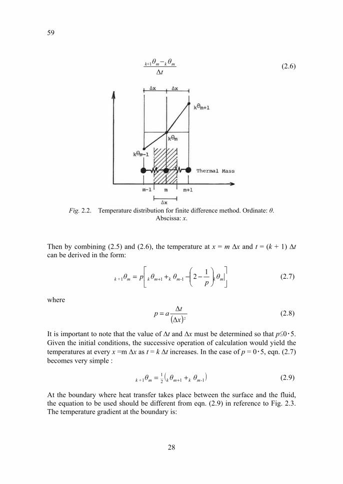
In solving eqn. (2.4) by the finite difference method, it is necessary first to convert every variable item in the differential equation into a finite form. Defining t = k ∆t and x = m ∆x where ∆t is time increment, ∆x is incremental length and k and m are integers, temperature θ(x, t) is to be expressed as kθm. Then, the temperature gradients from x = (m − 1) ∆x to m ∆x and from x = m∆x to (m + 1) ∆x are expressed as:
xθθ -mkmk
Δ1− and
xθθ mk-mk
Δ1−
respectively. This is illustrated in Fig. 2.2. The rate of change in the temperature gradient to the incremental length ∆x is
given by:
−−−+
xθθ
xθθ
x-mkmkmkmk
ΔΔΔ1 11 (2.5)
which is a converted form in finite difference of the right-hand side of eqn. (2.4). On the other hand, the left-hand side of eqn. (2.4) is the temperature gradient of
the thermal mass at x = m ∆x in reference to the time increment ∆t, thus the converted form can be expressed as:
59
28
tθθ mkmk
Δ1+ − (2.6)
Fig. 2.2. Temperature distribution for finite difference method. Ordinate: θ.
Abscissa: x.
Then by combining (2.5) and (2.6), the temperature at x = m ∆x and t = (k + 1) ∆t can be derived in the form:
−−+= + mk-mkmkm k θ
pθθpθ 12111+ (2.7)
where
( )2Δ
Δxtap = (2.8)
It is important to note that the value of ∆t and ∆x must be determined so that p≤0・5. Given the initial conditions, the successive operation of calculation would yield the temperatures at every x =m ∆x as t = k ∆t increases. In the case of p = 0・5, eqn. (2.7) becomes very simple :
( )1121
1+ -mkmk m k θθθ += + (2.9)
At the boundary where heat transfer takes place between the surface and the fluid, the equation to be used should be different from eqn. (2.9) in reference to Fig. 2.3. The temperature gradient at the boundary is:

60
29
αλxθθ
xt fkk
m +
−=
=
2ΔΔ
Δ 0
0 (2.10)
where kθ0 = average temperature of surface layer at time k (˚C), kθf = fluid temperature at time k (˚C), and α = film coefficient (W m-2 deg C-1).
Making m = 0 in eqn. (2.5) and replacing the second term of eqn. (2.5) by eqn. (2.10), k + 1θ0 can be obtained by the expression:
−+−+
+=p
xλθ
xλ
θθpθ k
fkk k
1
αΔ2+1
11
αΔ21
2 0101+ (2.11)
The above application of the finite difference method is called an explicit procedure and in practice it tends to require quite extensive computation time.
Fig. 2.3. Temperature distribution with boundary layer.
The implicit method is often used when computer calculation is applicable. In
this case instead of eqn. (2.6) the temperature gradient of (kθm − k−1θm)/∆t is introduced. Then the basic formula corresponding to eqn. (2.7) is expressed by:
−−
+= + 111+
12 -mkmkmkm k θθθp
pθ (2.12)

59
30
and at the boundary:
+−−
++
+=−
xλ
θθ
pxλθpθ fk
kk k
αΔ21
1
αΔ21
112 1001
(2.13)
It is necessary in this case to solve for kθm (m = 0, 1, 2,…) by simultaneous equations, but there is no requirement in the range of p. This reduces the computer time to a large extent in comparison with the explicit method.
2.3. PERIODIC STEADY HEAT CONDUCTION
A wall can be considered as a thermal system, when it receives an excitation such as change of outside air temperature or solar radiation incident on the outside surface and yields various kinds of response such as variation in the temperature distribution across it and in the heat flow through it. The excitation is quite random in the case of natural phenomena, but it can be idealised in such a way that outside air temperature varies and repeats over a period of 24h. In consequence, heat flow at the inside surface, room air temperature and all other variables should be varied over a period of 24h. Under these conditions the unsteady state heat conduction differential equation can be solved as a frequency response when the basic excitation is given in the form of cos ωt. If the actual excitation is given in the form of a Fourier series, it is easy to arrive at the actual form of response in a Fourier series.
The basic form of frequency response is expressed as η cos (ωt + μ), where η is called damping factor if excitation and response are in the same units and μ is called time lag.
Fourier’s series are defined as the series consisting of a multiple number of trigonometrical functions by which any functions could be approximated. For example, a function f(x) can be expressed in the form of the following, viz.,
∞∞
++=1=1=
cossin)f(n
n0n
n nxbbnxax (2.14)
60
31
where
ξ d)ξf(π1
ξ dξcos)ξf(π1
ξ dξsin)ξf(π1
ξ dξ2sin)ξf(π1
ξ dξsin)ξf(π1
π
π0
π
π
π
π
π
π2
π
π1
b
n b
n a
a
a
-
-n
-n
-
-
=
=
=
=
=
(2.14a)
In the case when f(x) is defined within the range of − l ≤ x ≤ l,
∞∞
++=1=1=
cossin)f(n
n0n
n lxπnbb
lxπnax (2.15)
where
ξ d)ξf(21
ξ dξsin)ξf(1
ξ dξsin)ξf(1
0
1
l
b
lπn
lb
lπn
la
l
l-
l
l-n
l
l-
=
=
=
(2.15a)
The function f(x) must not be infinity and must not have an infinite number of discontinuous points within the defined range.
The principle of periodic heat conduction through a wall is the following, When the excitation function is expressed by:
∞
+=1=
)cos()f(n
nn μtωnbt (2.16)
where t is time and ω is angular velocity (rad h-1), the temperature or the heat flow at point x and at time t can be obtained in the expression:
∞
++=1=
)](cos[)g(n
nnnn μγtωnPbt (2.17)
59
32
if the thermal properties of wall elements are given. The problem is to find a method to obtain Pn and γn. In order to do this, it is necessary only to determine the response g(t) in the form of:
)cos()g( γtωPt += (2.18)
against the basic excitation expressed by:
tω t cos)f( = (2.19)
Here g(t) is called as frequency response of f(t).
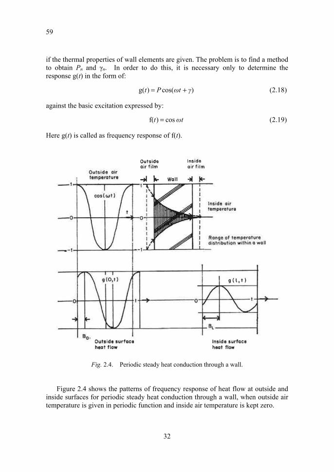
Fig. 2.4. Periodic steady heat conduction through a wall.
Figure 2.4 shows the patterns of frequency response of heat flow at outside and inside surfaces for periodic steady heat conduction through a wall, when outside air temperature is given in periodic function and inside air temperature is kept zero.

60
33
Maeda [2.1] solved the differential equation (eqn. (2.4)) under periodic steady conditions. The Frequency response of the temperature within the walls at x and at time t for flat single layer homogeneous wall derived by Maeda is expressed in the form:
θ(x , t) = P(x) cos {ωt + γ(x)} (2.20)
against the conditions that:
0)(cos)0( = t ,lθ
ωt = t ,θ (2.21)
where l is the wall thickness (m). P(x) and γ (x) are to be given in the following formulae, making:
aωA2
= (2.22)
)2(coscoshcos)2(cosh
sin)2(2sinh)(2cosh)(xlAAxAxxlA
AxxlAxlAxP−−−
−−−= (2.23)
)2(coscoshcos)2(cosh
sin)2(sinh)2(sinsinhtan)( 1
xlAAxAxxlAAxxlAxlAAxxγ−−−
−−−= −
(2.24)
The heat flow at the surfaces x = 0 and x = l is given in the following, viz.,
)Γcos(),0( 00 += tωAPλtq (2.25)
where
AlAl
AlAlP2cos2cosh
)2cosh2(cosh20 −
+= (2.26a)
Al2sinAl2sinhAl2sinhAl2sinh
0 +−=Γ (2.26b)
)cos(),( ll tωAPλtlq Γ+= (2.27)
where
AlAl
Pl 2cos2cosh2
−= (2.28a)
AlAlAlAlAlAlAlAl
l sinhcoscossinsinhcoscossinΓ
+−= (2.28b)
59
34
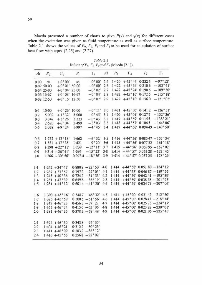
Maeda presented a number of charts to give P(x) and γ(x) for different cases when the excitation was given as fluid temperature as well as surface temperature. Table 2.1 shows the values of P0, Γ0, Pl and Γ1 to be used for calculation of surface heat flow with eqns. (2.25) and (2.27).
Table 2.1 Values of P0, Γ0, Pl and Γ1 (Maeda [2.1])
60
35
2.4. INDICIAL RESPONSE
Taking a section of a wall as a thermal system, the response coming from the system when the excitation is in the form of a unit function is called indicial response. Unit function U(t) is defined as the function of time characterised by:
U (t) = 0 for t ≤ 0 U (t) = 1 for t > 0
Figure 2.5. shows the unit function.
Fig. 2.5. Unit function.
The unit function is one of the basic excitation functions and the indicial response is the basic response function that characterises the system. Using the indicial response, the response to any excitation can be obtained by the convolution principle to be described later.
In the case of unsteady state heat conduction through a flat, homogeneous wall, the unit function and indicial response can be temperature or heat flow. It is always important, therefore, to specify the nature of these functions.
Let us take a unit function representing the surface temperature at x = 0, keeping the other surface temperature at x = l to be always 0, where l is wall thickness. Then the task is to obtain the response function of temperature within the wall section. The procedure to obtain such an indicial response is to solve the partial differential equation of unsteady state heat conduction of eqn. (2.4) under the conditions that
( )( ) 0,
)(U,0= t l θ
t= t θ (2.29)
It is known that the form of the solution equation, eqn. (2.4), is expressed by:
( ) ( )lxπntDCBAx= t x θ
nnn sinexp,
1
∞
=
−++ (2.30)
A, B, C and D are the unknown constants to be determined from the boundary conditions as given by eqn. (2.29) in this case. B = 1 can be derived from θ(0, t) = U(t) and Al + B = 0 from θ(l, t) = 0 that gives A = −1/l.
59
36
Substituting ∂θ/∂t and ∂2θ / ∂x2 from eqn. (2.30) into eqn. (2.4):
2
22
lπnaDn = (2.31)
can be obtained. From the condition θ(x, 0) = 0 and the above results, it follows that:
∞
=
=+−1
0sin1n
n lxnπC
lx (2.32)
Using the formula (2.15a) where f(x) = −1 + x/l, Cn can be obtained as:
−=
+−=
1
0
2sin12nπ
ξdlξnπ
lξ
lCn (2.33)
Then the solution is expressed by the following, denoting it as Φθ0(x, t):
( ) ∞
=
−−−=
12
22
0 sinexp1π21,Φ
nθ l
xnπtlπan
nlxtx (2.34)
This is the indicial response of the temperature of the wall section against the excitation of the surface temperature at x = 0. The rate of heat flow is derived from eqn. (2.34) and expressed as:
( ) ( )
−+=
∂∂−=
∞
=12
22
00
cosexp121
Φ,Φ
n
θq
lxnπt
lπan
nllλ
xtx,λtx
(2.35a)
The heat flow at x = l, which essentially becomes a characteristic function for heat gain through walls, is given by:
( ) ( )
−−+=
∞
=12
22
0 exp121,Φn
nq t
lπan
llλtl (2.35b)
In a similar manner, the indicial response of the temperature of the wall section to the excitation of the surface temperature at x = l can be obtained. It is denoted by Φθ1(x, t) expressed as:

60
37
( ) ( )∞
=
−−+=
12
22
0 sinexp12,Φn
n
θ lxnπt
lπan
πnlxtx (2.35c)
2.5. IMPULSE RESPONSE AND CONVOLUTION
Impulse response is simply a derivative of indicial response, viz.,
t
tx,tx,φd
)(Φd)( = (2.36)
where Φ(x, t) identifies indicial response and φ(x, t) impulse response. Two subscripts are used for Φ and φ in this book. The first subscript identifies the temperature or heat flow and the second subscript the location where temperature excitation is given; for example Φθ0 means the indicial response of temperature against temperature excitation at x = 0, and φq1 means the impulse response of heat flow against temperature excitation at x = l.
Impulse response is often called a weighting function and is also defined as the response against the excitation given in the form of Dirac’s delta function. The delta function δ(t) is again a derivative of the unit function, namely:
tttδ
d)(dU)( = (2.37)
and defined as the function of time characterized by:
ε
tδ 1)( = for 0 ≤ t ≤ ε
0)( =tδ for t < 0, t > ε (2.38)
( ) 1dlim00
=→
ε
εttδ
Figure 2.6 shows the delta function. Impulse response is also a characteristic function relating excitation to response. When the actual excitation is given in the form of a function of time f(t), the actual response g(t) is expressed in the following form, using impulse response for the system φ(t), viz.,
( )∞
−=0
d)f()(g ττtτφt (2.39)

59
38
Fig. 2.6. Delta function.
This form of integral expression is called convolution or Duhamel’s integral, and is a very important expression. It is always difficult for beginners to understand the real meaning of the convolution. One must bear in mind that the integral is a function of t not of τ and τ is also expressed in time domain, starting from τ =0 at time t to the reverse direction towards the past as shown in Fig. 2.7.
The product of φ(τ)f(t − τ)dτ corresponds to the shaded volume in Fig. 2.7. The excitation that appeared τ ago from the present time t brings effect at t as a part of the response at t.
Fig. 2.7. Graphical interpretation of convolution.
So the integral is the sum of these effects of incremental responses from τ = 0 to
infinity, which corresponds to the total volume of Fig. 2.7, making the actual response g(t) of eqn. (2.39).
The impulse response of the surface heat flow at x = 0 and x = l against the

60
39
surface temperature excitation at x = 0 can be obtained by differentiation from eqn. (2.35a) as follows:
( )
−−=
∞
=
tlπan
lπanλtφ
nq 2
22
2
22
10 exp2,0 (2.40)
( ) ( )
−−−=
∞
=
tlπan
lπanλtlφ
n
nq 2
22
2
22
10 exp12, (2.41)
Figure 2.8 shows the generalised pattern of the impulse response of the inside surface heat flow against the surface temperature excitation at x = 0 and x = l.
For example, the surface heat flow at x = l, q(l, t), when the surface temperature excitation at x = 0 is given as f(t) = −ct2 , can be obtained from the calculation of the fo1lowing convolution, viz.,
( ) ( ) ( )[ ]
( ) ( )
( )
∞
=
∞
=
∞
∞
=
∞
−−=
−
−−−=
−−
−−−=
12
22
2
12
22
02
22
2
12
22
0
12
dexp12
dexp12,
n
n
n
n
n
n
I.lπanλc
ττt.τlπan
lπanλc
ττtcτlπanλtlq
Letting
klπan =2
22
Fig. 2.8. Impulse response of inside heat flow for surface temperature excitation,
and

59
40
( )( )
( )kIt
ττtτk k τtτk
ττtτkI
+−=
−−−−−−=
−−=
∞∞
∞
331
2
003
31
0
d))(exp(])[exp(
dexp
Therefore,
−
=−
=13
)1(32
22
33
lπant
ktI
and thus
(2.42)
2.6. SOLUTION BY LAPLACE TRANSFORMATION
Solution of the partial differential equation of unsteady state heat conduction in a flat wall by the method of Laplace transformation is described in various text books such as those by Carslaw and Jaeger [2.2] and Churchill [2.3].
The Laplace transformation is a very convenient tool for solving differential equations. The method of solution appears quite easy as if it were solved by a trick. It is made in the same way as a multiplication is performed by the operation of an addition in the imaginary space of logarithm, where ‘log’ is called operator. In the case of the Laplace transformation, every term in a differential equation is transformed into another form within an imaginary space according to a certain rule by the operator ‘L’, so that the differential equation in the original space is transformed into a simple algebraic equation in the imaginary space and can be solved quite easily. The solution in the imaginary space is then transformed back into the form of the original space by the same rule to become a solution function.
( ) ( )
⋅⋅⋅+−
−−
+−
−=
−
−−= ∞
=
2
2
2
2
2
23
32
2
22
3
12
22
91
1
41
1
1
1
1312,
πal
πal
πal
tλc
lπant
lπanλctlq
n
n

60
41
The rules for the transformation are rather simple. By definition the original function f(t) of time t, is transformed into φ(s) in the imaginary space according to the formula:
∞
−=0
d)(exp)(f)( t st tsφ (2.43)
The function φ(s) is called the Laplace transform of f(t) and may be denoted as:
)(})L{f( sφt = (2.44)
There are some fundamental rules of Laplace transformation as follows: (1) )()(})(f{L})(f{ L})(f)(fL{ 212121 sbφsaφtbtatbta +=+=+
(2.45) where a and b are constants.
= sφ(s) − f(0) (2.46) (2) L where f(0) is value of f(t) at t = 0
= snφ(s) − sn−1f(0) − sn−2f′(0) − … − f(n−2)(0) (2.47) (3) L
= φ(s)s1 (2.48) (4) L
(5) )()}(fL sφ t t −={ (2.49) (6) )()}(f)exp(L asφtat −={ (2.50)
= )()( 21 sφ . sφ (2.51) (7) L
After solving an equation for φ(s), φ(s) must be transformed back into f(t). The fundamental relationships of reverse transformation are listed in Table 2.2.
The partial differential equation of the unsteady state heat conduction as in eqn. (2.4) can be rewritten in the form of imaginary space by the rules of Laplace transformation, making L{θ (x, t)} = u(x, s) as in the following:
t t
∂∂ )(f
n
n
t t
∂∂ )(f
t
ττ0
d)(f
−t
τττt0 21 d)(f)(f

59
42
)()(2
2
sx,sux
sx,ua =∂
∂ (2.52)
The solution form of this equation is
)(exp)(exp)( 221 xd cxd, csx,u −+= (2.53)
where cl, c2, dl and d2 and determined by boundary conditions. When the boundary conditions are u(0, s) = 0 and u(l, s) = f(s), it follows that:
)(exp)(exp)(f
)(exp)(exp)(f
2
1
21
aslaslsc
aslaslsc
asdd
−−−=
−−=
==
Then the solution of eqn. (2.52) is expressed by:
)()(sinhsinh
)()( 1 sx,φsfaslasx
sfsx,u θ== (2.54)
where
aslasx
sx,τθ sinhsinh
)(1 = (2.55)
τθ1 (x, s) is the Laplace transform of the impulse response of the temperature at x against the surface temperature excitation at x = l and is called the transfer function. In general, the transfer function may be defined as the Laplace transform of the impulse response. The transfer function could also be interpreted as the solution when excitation is given as a delta function in the original space, i.e. f(s) = 1 as one of the boundary conditions. Reverse transform of τθ1 (x, s) gives impulse response as in the following, viz.,
lxπnt
lπan n
laπ
aslasx
sx,τ
x
n
n
θ
sinexp)1(2
sinhsinh
)(
2
22
12
1
−−−=
=
=
(2.56)
It is obvious that this is the derivative of eqn. (2.35).

60
43
Table 2.2 Reverse transformation of simple functions
59
44
Table 2.2―contd.
2.7. MATRIX EXPRESSION OF SURFACE TEMPERATURE AND SURFACE HEAT FLOW
In the air conditioning load calculation, we are interested in the temperature and heat flow particularly at both surfaces of the wall. When the temperature excitation is given on both surfaces at x = 0 and x = l in the expression θ(0, t) and θ(l, t) simultaneously, the superposition principle yields the equations to give the heat flow at both surfaces as in the following convolution expression:
−+−=x
q
x
q ττtl,θ τφ τ τtθ τφ t,q0 10 0 d)(.),0(d),0(.),0()0(
(2.57)
−+−=x
q
x
q ττtl,θ τlφ τ τtθ τlφ tl,q0 10 0 d)(.),(d),0(.),()(
(2.58)
In converting these equations into Laplace transform, the following notations are to be used:
,),(}),(L{,),(}),(L{
00 sxτtxφsxutxθ
qq ==
,),(}),(L{,),(}),(L{
11 sxτtxφsxhtxq
qq ==
(2.59)
Then eqns. (2.57) and (2.58) can be rewritten in the following Laplace transform applying the formula that convolution becomes a product in the imaginary space as shown in eqn. (2.51).

60
45
),(),(),0(),(),(),(),0(),0(),0(),0(
10
10
slu slτsu slτsl hslu sτsu sτs h
+=
+= (2.60)
These can be rewritten in matrix expression as follows,
slu su
slτ slτ
sτsτsl hs h
=
),(),0(
),(),(),0(),0(
),(),0(
10
10
(2.61)
The first matrix in the right-hand side of the above expression is called transfer matrix, in the sense that it relates the temperature matrix to the heat flow matrix. This is analogous to the relationship between electric current and voltage in a system as explained by Pipes [2.4]. The four elements of the transfer matrix can be obtained from the transfer function of temperature given in eqn. (2.55). The relation between the transfer function of heat flow and the transfer function of temperature is the same as in the original space, viz.,
aslasx
asλ
xsx,τλsx,τ θ
q
sinhcosh
)()( 11
−=
∂∂−=
Therefore
aslasl
asλsl,τ
aslasλ
s,τ
q
q
sinhcosh
)(
sinh)0(
1
1
−=
−=
(2.62)
Similarly,
aslasxl
asλ
aslasxl
xλ
xsx,τλsx,τ θ
q
sinh)cosh(
sinh)sinh()()( 0
0
−−=
−∂∂−=
∂∂−=
Therefore,

59
46
aslasλ
sl,τ
aslasl
asλs,τ
q
q
sinh)(
sinhcosh
)0(
0
0
=
=
(2.63)
It must be noted that:
)0()(
)()0(
01
01
s,τsl,τsl,τs,τ
=
= (2.64)
Furthermore eqn. (2.61) can be rewritten as
sl hslu
sDsCsBsA
s hsu
=
),(),(
)()()()(
),0(),0(
(2.65)
where
asl
slτsτ
sD
asl
asλsτ
slτslτ
sτsC
asλasl
slτsB
asl
slτslτ
sA
q
q
q
q
q
cosh),(),0(
)(
sinh),0(),(),(
),0()(
sinh),(
1)(
cosh),(),(
)(
0
0
00
11
0
0
1
==
−=−=
==
==
(2.66)
The meaning of eqn. (2.65) is that it gives responses of temperature and of heat flow at one surface when both excitations of temperature and heat flow at the other surface affect the thermal system of a wall section as characterised by the transfer matrix.
For the wall whose thermal capacity can be neglected, i.e. 1/α =0, the transfer matrix in eqn. (2.65) can be reduced to the following:
R
sD sC
sBsA
10
1)()()()(
(2.67)
Where R = thermal resistance (m2degC W−1). For a multi-layer wall, the transfer matrix of the whole wall is to be expressed

60
47
simply by the product of the transfer matrices of every layer of the wall. Thus, using simplified notation,
⋅⋅⋅
=
1
1
22
22
11
11
0
0
hu
DCBA
DCBA
DCBA
hu
m m
m m
(2.68)
Having the product of these transfer matrices converted into one transfer matrix, the relationship of surface temperature and heat flow between at one surface of a multi-layer wall and at the other surface of it can be expressed in the same form as in the case of single layer wall, namely:
=
1
1
0
0
hu
DCBA
hu
(2.69)
When the boundary layer of surface film is to be taken into account, i.e. excitation and response are given in fluid temperature instead of surface temperature, the procedure is so simple that the first and the last transfer matrices need only be substituted by the matrix for the layer without thermal capacity as expressed by eqn. (2.67).
After obtaining the combined transfer matrix as expressed by eqn. (2.69), it is necessary to convert back into the original form as in eqn. (2.61) in order to have the surface heat flows expressed as responses and the surface temperatures as excitations. Thus the final form of a multi-layer wall is expressed in the following:
=
1
0
1
0
)()(
)(1
)(1
)()(
u u
sBsA
sB
sBsBsD
h h
(2.70)
The problem is then to transform the four elements in the matrix back into their original form in the original space.
2.8. RESPONSE FACTORS―DEFINITION AND USAGE
In order to make use of eqn. (2.70) to obtain surface heat flow as heat gain through a wall, temperature excitation should be given as an algebraic function which can be transformed easily into the Laplace imaginary form, although the calculation process in the convolution can still be complicated.
Mitalas and Stephenson [2.5] presented an approach which introduced a time series expression into the calculation process. Looking at the natural excitations such
59
48
as outside air temperature and solar radiation, they were found to vary in a quite random fashion. It is necessary, therefore, to incorporate these natural random processes into the thermal system if a rather rigorous manipulation of theoretical process is to be made, as discussed so far.
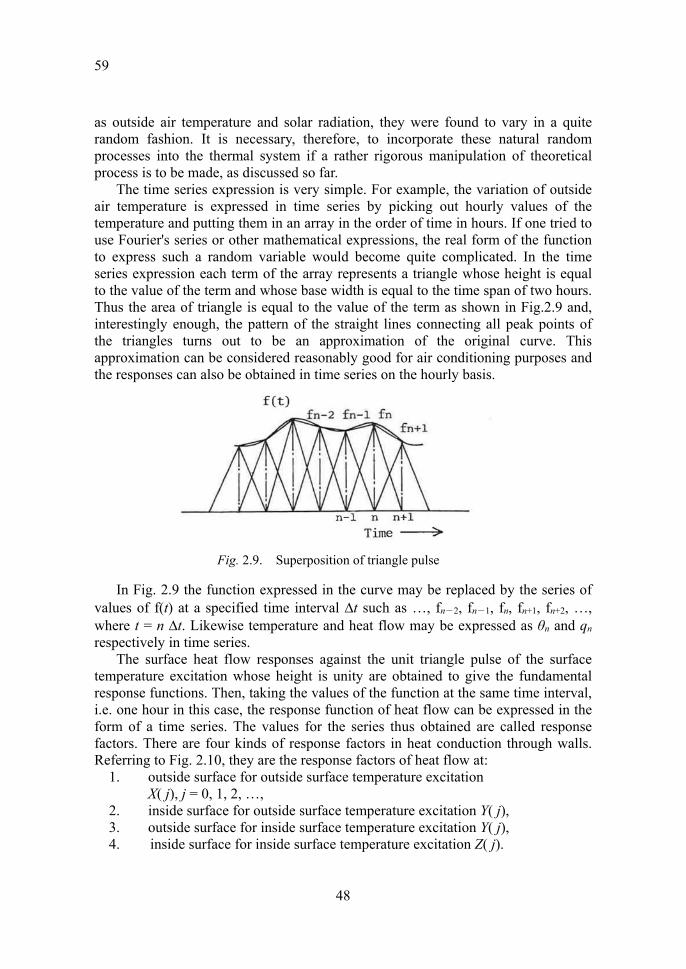
The time series expression is very simple. For example, the variation of outside air temperature is expressed in time series by picking out hourly values of the temperature and putting them in an array in the order of time in hours. If one tried to use Fourier's series or other mathematical expressions, the real form of the function to express such a random variable would become quite complicated. In the time series expression each term of the array represents a triangle whose height is equal to the value of the term and whose base width is equal to the time span of two hours. Thus the area of triangle is equal to the value of the term as shown in Fig.2.9 and, interestingly enough, the pattern of the straight lines connecting all peak points of the triangles turns out to be an approximation of the original curve. This approximation can be considered reasonably good for air conditioning purposes and the responses can also be obtained in time series on the hourly basis.
In Fig. 2.9 the function expressed in the curve may be replaced by the series of
values of f(t) at a specified time interval ∆t such as …, fn-2, fn-1, fn, fn+1, fn+2, …, where t = n ∆t. Likewise temperature and heat flow may be expressed as θn and qn respectively in time series.
The surface heat flow responses against the unit triangle pulse of the surface temperature excitation whose height is unity are obtained to give the fundamental response functions. Then, taking the values of the function at the same time interval, i.e. one hour in this case, the response function of heat flow can be expressed in the form of a time series. The values for the series thus obtained are called response factors. There are four kinds of response factors in heat conduction through walls. Referring to Fig. 2.10, they are the response factors of heat flow at:
1. outside surface for outside surface temperature excitation X( j), j = 0, 1, 2, …,
2. inside surface for outside surface temperature excitation Y( j), 3. outside surface for inside surface temperature excitation Y( j), 4. inside surface for inside surface temperature excitation Z( j).
Fig. 2.9. Superposition of triangle pulse

60
49
Fig. 2.10. Response factors [7.4].
These surface temperature excitations are given in the form of a unit triangular pulse. Response factors also characterise the thermal system of a wall as do the transfer function and the impulse response. The convolution expression in time series then allows for calculation of actual response of the surface heat flow as in the following.
When the surface temperature at x = 0 is given in time series as …, θ(n−2), θ(n−1), θ(n), the responses of surface heat flow at time t = n ∆t at x = 0 and x = l due to these temperatures can be expressed by using response factors X(j) and Y(j) as follows:
(2.71)
(2.72)
When the surface temperature at x = l is given as θ(n), the responses of surface heat flow are expressed in the following, taking the direction of heat flow reversed:
∞
=
−=0
1 )()(),0(j
jnθjYnq (2.73)
∞
=
−=0
1 )()(),(j
jnθjZnlq (2.74)
These are the fundamental convolution forms using response factors. The real problem is then how to obtain response factors.
∞
=
∞
=
−=
⋅⋅⋅+−+−+=
−=
⋅⋅⋅+−+−+=
0
0
0
0
)()(
)2()2()1()1()()0(),(
)()(
)2()2()1()1()()0(),0(
j
j
jnθjY
nθYnθYnθYnlq
jnθjX
nθXnθXnθXnq

59
50
2.9. DERIVATION OF RESPONSE FACTORS The core equation from which the response factors are derived is the matrix equation in the Laplace imaginary form as expressed in eqn. (2.70) for a general multi-layer wall. The response factors X(j), Y(j) and Z(j) are expressed in time series of the function of t as the reverse transform of
)s(B)s(A
)s(B1
)s(B)s(D and
respectively, when u0 and u1 are given in the Laplace transform of the unit triangle surface temperature. The unit triangle pulse for a given time increment ∆t as shown in Fig. 2.11 can be expressed by the superposition of three ramp functions:
)Δ(Δ1
Δ2)Δ(
Δ1)(f tt
tt
ttt
tt −+−+= (2.75)
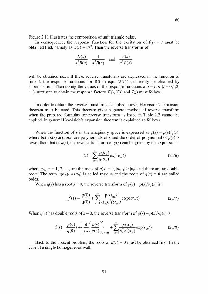
Fig. 2.11. Composition of unit triangle pulse [7.4]. (a) Unit function, (b) ramp function,
(c) (1/∆t)(t+∆t), (d)-2t/∆t, (e) (1/∆t)(t-∆t), (f) unit triangle pulse as (c) + (d) + (e).
60
51
Figure 2.11 illustrates the composition of unit triangle pulse. In consequence, the response function for the excitation of f(t) = t must be
obtained first, namely as L{t} = l/s2. Then the reverse transforms of
)(
)(and)(
1)(
)(222 sBs
sAsBssBs
sD
will be obtained next. If these reverse transforms are expressed in the function of time t, the response functions for f(t) in eqn. (2.75) can easily be obtained by superposition. Then taking the values of the response functions at t = j ∆t (j = 0,1,2,…), next step to obtain the response factors X(j), Y(j) and Z(j) must follow.
In order to obtain the reverse transforms described above, Heaviside’s expansion theorem must be used. This theorem gives a general method of reverse transform when the prepared formulas for reverse transform as listed in Table 2.2 cannot be applied. In general Heaviside’s expansion theorem is explained as follows.
When the function of s in the imaginary space is expressed as φ(s) = p(s)/q(s), where both p(s) and q(s) are polynomials of s and the order of polynomial of p(s) is lower than that of q(s), the reverse transform of φ(s) can be given by the expression:
)exp()()()(f
1tα
αqαpt m
m m
m∞
=
= (2.76)
where αm, m = 1, 2, …, are the roots of q(s) = 0, |αm+1| > |αm| and there are no double roots. The term p(αm)/ q′(αm) is called residue and the roots of q(s) = 0 are called poles.
When q(s) has a root s = 0, the reverse transform of φ(s) = p(s)/sq(s) is:
)texp(q
p)0(q)0(p)t( m
1m mm
m ααα
α∞
= ′+=
)()(f (2.77)
When q(s) has double roots of s = 0, the reverse transform of φ(s) = p(s)/sq(s) is:
)exp()(
)()()(
dd
)0()0()(f
12
0
tααqααp
sqsp
s t
qpt m
m mm
m
s
∞
== ′+
+= (2.78)
Back to the present problem, the roots of B(s) = 0 must be obtained first. In the case of a single homogeneous wall,
59
52
asλ
aslssBs
sinh)( 22 = (2.79)
The roots of 0sinh =s/al are
2
22
laπmαm −= (2.80)
This implies that all of the roots are negative real. There are also double roots of s = 0 from s2 = 0. Then the reverse transform of D(s)/s2B(s) can be expressed using the formula of eqn. (2.78) as in the following:
)exp()(
)()()(
dd
)0()0()(ξ
12
0
tααBααD
sqsD
st
BDt m
m mm
m
s
∞
==′
+
+= (2.81)
The response factors X(j) are then obtained as follows:
2for]Δ)1ξ[()Δξ (2]Δ)1ξ[()(
)Δξ (2)Δ2ξ ()1()Δξ ()0(
≥++−+=−=
=
jtjtjtjjXttX
tX
(2.82)
Similarly η(t) and ζ(t) can be expressed as the reverse transform of 1/s2B(s) and A(s)/s2B(s) respectively, in the form as functions of t similar to eqn. (2.81) and the response factors Y(j) and Z(j) are obtained in the same way as in eqn. (2.82).
In the case of a multi-layer wall, the form of B(s) is not so simple as in eqn. (2,79). The original method of finding the roots in the case of the multi-layer wall is presented by Mitalas and Arseneault [2.6].
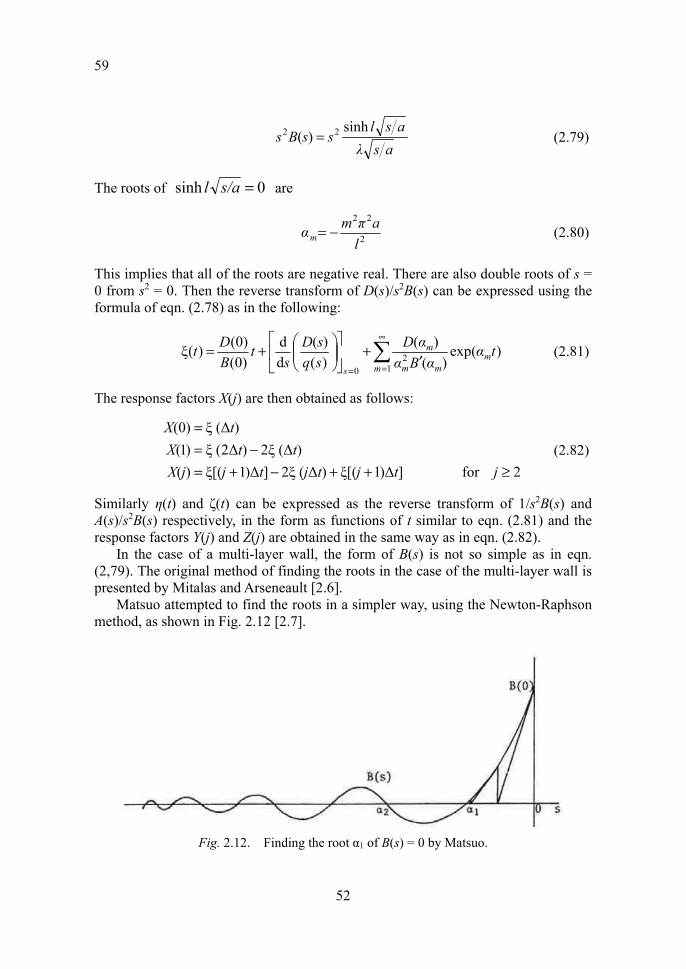
Matsuo attempted to find the roots in a simpler way, using the Newton-Raphson method, as shown in Fig. 2.12 [2.7].
Fig. 2.12. Finding the root α1 of B(s) = 0 by Matsuo.
60
53
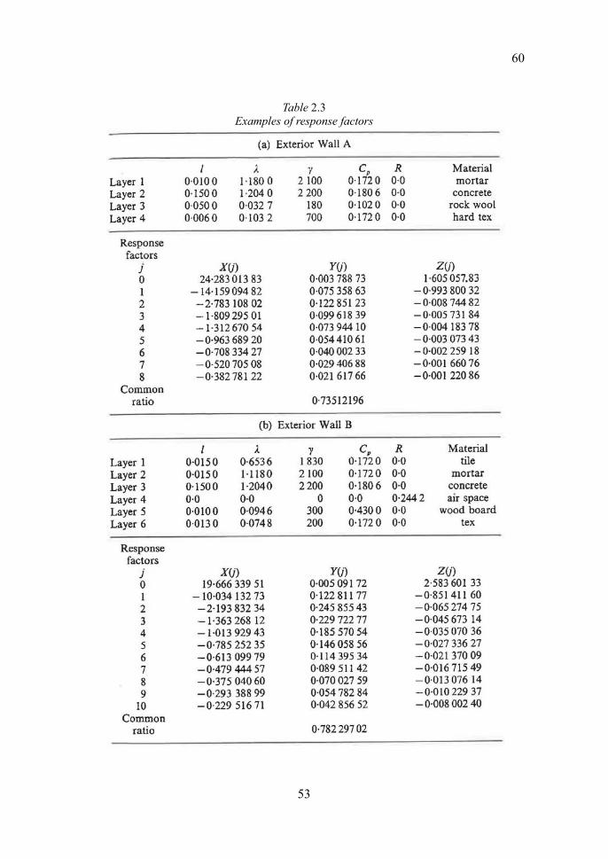
Table 2.3 Examples of response factors

59
54
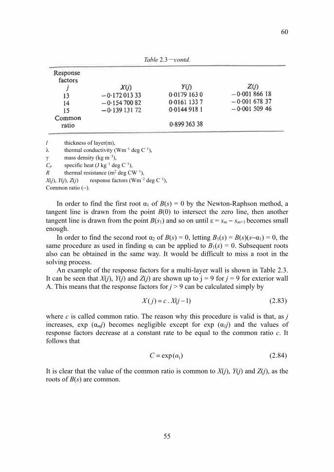
Table 2.3―contd.
60
55
Table 2.3―contd.
l thickness of layer(m), λ thermal conductivity (Wm-1 deg C-1), γ mass density (kg m-3), Cp specific heat (J kg-1 deg C-1), R thermal resistance (m2 deg CW-1), X(j), Y(j), Z(j) response factors (Wm-2 deg C-1), Common ratio (−).
In order to find the first root α1 of B(s) = 0 by the Newton-Raphson method, a tangent line is drawn from the point B(0) to intersect the zero line, then another tangent line is drawn from the point B(s1) and so on until ε = sm − sm+1 becomes small enough.
In order to find the second root α2 of B(s) = 0, letting B1(s) = B(s)(s−α1) = 0, the same procedure as used in finding αl can be applied to B1(s) = 0. Subsequent roots also can be obtained in the same way. It would be difficult to miss a root in the solving process.
An example of the response factors for a multi-layer wall is shown in Table 2.3. It can be seen that X(j), Y(j) and Z(j) are shown up to j = 9 for j = 9 for exterior wall A. This means that the response factors for j > 9 can be calculated simply by
)1(.)( −= jX cjX (2.83)
where c is called common ratio. The reason why this procedure is valid is that, as j increases, exp (αmj) becomes negligible except for exp (α1j) and the values of response factors decrease at a constant rate to be equal to the common ratio c. It follows that
)(exp 1αC = (2.84)
It is clear that the value of the common ratio is common to X(j), Y(j) and Z(j), as the roots of B(s) are common.

59
56
2.10 PRACTICAL APPLICATION OF RESPONSE FACTORS The theoretical formula to obtain the response of surface heat flow g(n) from the excitation of surface temperature f(n) using response factors is expressed by definition as:
)(f)()g(0
jn . jYnj
−=∞
=
(2.85)
In practice, however, the summation must be limited up to a certain large number instead of infinity. Even if the sum of 50 products of Y and f are made, a truncation error still possibly exists. Moreover, this summation of products requires quite a lot of computation time.
There is a method to avoid making the summation of as many products of Y and f without losing accuracy. Using the common ratio c of Y(j), eqn. (2.85) may be rewritten as:
(2.86)
Substituting n − 1 into n of eqn. (2.86), it gives:
)1(f)()1(f)()1g(10
jknckYjnjYnj
jk
j
−−−+−−=− ∞
==
(2.87)
Making a subtraction g(n) − c g(n − 1), it follows that:
{ } )jn( )1j(Y)j(Y)n()0(Y)1n( cnk
1j−−−++−=
=
ffg)g( (2.88)
Thus it is evident that eqn. (2.88) represents the practical formula to obtain g(n), the response at time n, from the limited small number of convolutions by making use of g(n − 1); the response at time n − 1, which is naturally considered to be a known value as the calculation of eqn. (2.88) should proceed with time. In other words, it can be understood that the previous response involves the convolution for j > k. This is the reason why operation of computation with eqn. (2.88) contributes a substantial reduction in computer time for practical use.
Further simplification may be conceivable from eqn. (2.88) in the following way. Letting:
)jkn( c)k(Y)jn()j(Y
)2kn(k(Yc)1kn(k(cY)kn()k(Y)1n()1(Y)n()0(Yn
1j
jk
0j
2
−−+−=
⋅⋅⋅+−−+−−+
−+⋅⋅⋅+−+=
∞
==
ff
)f)ffff)g(
60
57
)1(g)g ()(g
)0 ()0(1for)1() ()(
−−=′=′
≥−−=′
ncnnYY
jjcYjYjY
(2.89)
eqn. (2.88) may be rewritten as:
)(f)()(g0
jnjYnk
j
−′=′ =
(2.90)
Taking a common ratio of Y′(j) as c′,
)jn()]1j(Yc)j(Y[)n()0(Y)1n(cnk
1j−−′′−′+′+−′′=′
′
=
ffg)(g
(2.91) This is entirely the same form as eqn. (2.88) but k′ < k and the total operation of multiplication to obtain g(n) is consequently shorter than the case if eqn. (2.88) was used. In a similar manner further modification may be considered by making:
)1() ()( −′′−′=′′ jYcjYjY (2.92)
It can thus be modified further on. Experiences have shown, however, that the use of eqn. (2.88) is adequate enough
for calculation of cooling load of buildings, where there are not such thick walls. The latter procedure may well be applicable to the case when a large mass comes into the thermal system.
2.11. Z-TRANSFORM The advanced way of convolution is represented by so-called Z-transform, which is often used in the numerical control in random process. The basic formula of Z-transform to relate the output time series g(n) to the input time series f(n) is expressed by the following, viz.,
⋅⋅⋅+−+−+ )2(f)1(f)f( 210 nanana ⋅⋅⋅+−+−+= )2(g)1(g)g( 210 nbnbnb (2.93)
where a and b are the coefficients characterising the thermal system. Then the output g(n) can be given by:
⋅⋅⋅+−+−+= )2(f)1(f)(f)g( 2100 nanananb ])2(g)1(g[ 21 ⋅⋅⋅+−+−− nbnb (2.94)

59
58
Fig. 2.13. Sample values of f(t) taken at time interval of ∆.
Equation (2.94) means that the output at time n can be obtained by knowing the
output history. It can be derived from the following concept. In general, the Laplace transform of f(t), a function of time t, is expressed by
definition as:
tst tsφ d)(exp)(f)(0
−= ∞
(2.95)
Letting f(0), f(∆), f(2∆), … be the values of f(t) sampled at every ∆ hours as shown in Fig. 2.13, the Laplace transform of f(n) can be given by
⋅⋅⋅+−+−+= )Δ2exp()Δ2(f)Δexp()Δ(f)0(f)( sssφ )Δexp()Δ(f snn −+ (2.96)
Then the following expression with a function of z, when exp (∆s) = z in eqn. (2,96), is defined as the Z-transform of f(t), taking ∆ = 1, viz.,
nznzzz −−− +⋅⋅⋅+++= )(f)2(f)1(f)0(f)(F 21 (2.97)
If f(t) is the input function to a system given by eqn. (2.97) and g(t) is the output function given by:
nznzzz −−− +⋅⋅⋅+++= )(g)2(g)1(g)0(g)(G 21 (2.98)
the relationship between F(z) and G(z) is expressed as:
)()(F)(G zK
zz = (2.99)

60
59
where K(z) is called a Z-transfer function given by:
22
110
22
110)( −−
−−
++++=
zbzbbzazaazK (2.100)
When the system characteristics are known, the relationship between input time series f(n) and output time series g(n) can be expressed by substituting eqns. (2.97), (2.98) and (2.100) into eqn. (2.99) as follows:
]][)(f)1(f)1(f)0(f[ 110
)1(1 ⋅⋅⋅+++−+⋅⋅⋅++ −−−−− zaaznznz nn ])(g)1(g)1(g)0(g[ )1(1 nn znznz −−−− +−+⋅⋅⋅++= ][ 1
10 ⋅⋅⋅++× −zbb (2.101)
Equating the coefficients of z−n on both sides of eqn. (2.101), it follows that:
⋅⋅⋅+−+−+ )2(f)1(f)(f 210 nanana ⋅⋅⋅+−+−+= )2(g)1(g)(g 210 nbnbnb (2.102)
Then the output at time n, g(n), can be obtained from eqn. (2.102) as expressed in eqn. (2.94). Note that b0 = 1 always.
The coefficients a(j), b(j) are called Z-transfer factors and can be obtained directly from the formula for any type of multi-layer walls as described by Stephenson and Mitalas [2.9]. A computer program to obtain Z-transfer factors has been prepared by Mitalas and Arseneault [2.10]. The nature of the Z-transfer factors can be understood as described below, as they are related to the response factors.
Corresponding to the response factors X(j), Y(j) and Z(j) of a multi-layer wall, Z-transfer factors of A(j), B(j), C(j) and D(j) can be expressed by the following relationships:
=
−=j
i
ijDiXjA0
)()()( (2.103)
=
−=j
i
ijDiYjB0
)()()( (2.104)
=
−=j
i
ijDiZjC0
)()()( (2.105)
where i =1, 2, …, M.

59
60
D(j) can be obtained from the following:
∏∞
=
−−− −−=⋅⋅⋅+++1
121 )]Δexp(1[)2()1(1n
nαzzDzD (2.106)
Where αn are the roots of B(s) which appear in the inverse transform process for calculating response factors as discussed in the preceding section.
The Z-transfer factors can be used to calculate an output time series knowing an input time series. If the outside surface temperature is given by θ(n) in time series, the heat flow at the inside surface q(n) can be obtained from the following expression, viz.,
==
−−−=N
j
M
j
jnq jDjnθjBnq10
)(.)()()()( (2.107)
It is important to note that the number of summations of the products is limited in the above expression instead of being infinite as in the case of response factors. This allows for a more precise computation with a shorter convolution operation.
Donald G. Stephenson (1927-2009)
Dr. Stephenson is a native Canadian building physicist, well known for originator of response factors in building heat transfer. He received Ph.D. from University of Toronto. He devoted his whole life in heat transfer in buildings as Head of Building Services Section at Division of Building Research (DBR-IRC), National Research Council in Ottawa, where the author spent two years from 1967 as a postdoctorate fellow under his supervision. He wrote Chapter on Heat Load Calculation of ASHRAE Handbook of Fundamentals. ASHRAE Fellow. Father of five children.