unsteady shear layer roll up modeling - core.ac.uk · for obtaining the degree of master of science...

Unsteady Shear Layer Roll-Up

Modeling

Vortex Lattice Method

2

Unsteady Shear Layer Roll-Up

Modeling

Vortex Lattice Method

MASTER OF SCIENCE THESIS

For obtaining the degree of Master of Science in Computational Mechanics at

National Technical University of Athens

Theodore Ioannou M.Sc.

October 2016

Supervisor: Professor Gerasimos Politis

Committee:

Associate Professor Kostas Belibassakis

Assistant Professor Vasilis Riziotis

Faculty of Chemical Engineering ● National Technical University of Athens

3

Dedicated to

Dionysia,

Theodoros,

Vasilios

4

Acknowledgements

For the completion of the master thesis I would like to thank first and foremost my

family, who stood by me, always believed in my capabilities and encouraged me

throughout this endeavor. I would also like to thank my supervisor Professor

Gerasimos Politis, who was always there to guide me and without his valuable

support this thesis would have never been completed. Special thanks, to Mr.

Charalmpos Damianidis for his assistance with the visualization of some graphs.

5

Table of Contents

Acknowledgements .................................................................................................... 4

List of Figures ............................................................................................................. 8

Introduction .............................................................................................................. 10

Chapter 1 Main Considerations ............................................................................. 12

1.1 Definition of Frame of Reference ..................................................................... 12

Inertial Frame of Reference .................................................................. 12

Non-Inertial Frame of Reference .......................................................... 15

1.2 Motion and the No-Entrance Condition ............................................................ 20

Sinusoidal gust ..................................................................................... 21

Heaving motion ..................................................................................... 25

Pitching Motion ..................................................................................... 28

1.3 Vortex Lattice Method (VLM)............................................................................ 31

Representation theorems ..................................................................... 31

Grid discretization ................................................................................. 37

Linear system of equations ................................................................... 41

Chapter 2 Describing the Method .......................................................................... 44

2.1 Equations used in our modeling ....................................................................... 44

2.2 Modeling of vorticity ......................................................................................... 47

2.3 Time discretization ........................................................................................... 52

2.4 Wake panels modeling ..................................................................................... 53

6

2.5 The no-entrance boundary condition ................................................................ 55

2.6 Calculation of pressure difference and forces .................................................. 55

2.7 Pressure type Kutta condition .......................................................................... 65

Chapter 3 GPP, MPP and VLWU codes ............................................................... 67

3.1 Basic modules of the code ............................................................................... 67

Module nrtype ....................................................................................... 67

Module vector algebra .......................................................................... 67

3.2 GPP and MPP code ......................................................................................... 68

System_geometry_and_motion_flatwing program ................................ 69

Subroutine read_parameters ................................................................ 69

Subroutine wing_motion ....................................................................... 70

Subroutine create_c0_t......................................................................... 70

Subroutine write_system_geometry_at_time_t ..................................... 70

Subroutine tecplot ................................................................................. 70

3.3 The VLWU code ............................................................................................... 70

Subroutine read_parameters ................................................................ 70

Subroutine read_system_geometry_at_time_t ..................................... 71

Subroutine create_c1_t......................................................................... 71

Subroutine tecplot ................................................................................. 71

Subroutine Vorlin .................................................................................. 71

7

Subroutine Gelg .................................................................................... 71

Subroutines WFORCE, WPITCH, WHEAVE ........................................ 71

Chapter 4 Presentation of results .......................................................................... 72

4.1 VLWU code vs Theoretical data ....................................................................... 72

Sinusoidal gust on a thin airfoil ............................................................. 74

Thin airfoil performing a heaving motion ............................................... 76

Thin airfoil performing a pitching motion ............................................... 78

Influence of grid discretization .............................................................. 80

Influence of time discretization .......................................................... 83

Influence of Aspect ratio .................................................................... 84

4.2 Wake visualization ........................................................................................... 85

Wake visualization (Frozen wake model) ............................................. 86

Wake visualization (Free wake model) ................................................. 90

Chapter 5 Conclusions and future work ................................................................ 94

References ............................................................................................................... 95

8

List of Figures

FIGURE 1 RIGHT-HANDED FRAME OF REFERENCE .......................................................... 13

FIGURE 2 MOVING FRAME OF REFERENCE WITH RESPECT TO A STATIONARY FRAME OF

REFERENCE......................................................................................................... 13

FIGURE 3 MOVING NON-INERTIAL FRAME OF REFERENCE WITH RESPECT TO A MOVING

INERTIAL FRAME OF REFERENCE ............................................................................ 17

FIGURE 4 ROTATING NON-INERTIAL FRAME OF REFERENCE ............................................. 18

FIGURE 5 SINUSOIDAL GUST AND A MOVING WING .......................................................... 21

FIGURE 6 DEFINITION OF ANGLES WITH RESPECT TO A BODY-FIXED OBSERVER [43] .......... 24

FIGURE 7 SUCCESSIVE POSITIONS OF A DELTA WING PERFORMING A HEAVING MOTION ..... 26

FIGURE 8 SUCCESSIVE POSITIONS OF A RECTANGULAR WING PERFORMING A PITCHING

MOTION ............................................................................................................... 29

FIGURE 9 MOVING WING AND ITS TRAILING WAKE [15] .................................................... 32

FIGURE 10 MEAN CAMBER LINE OF A WING'S SECTION [15] ............................................. 35

FIGURE 11 DEFINITION OF THE KUTTA STRIP ................................................................. 37

FIGURE 12 DEFINITION OF GEOMETRY AND VORTEX PANEL ............................................. 38

FIGURE 13 DISTINCTION BETWEEN WAKE PANELS AND KUTTA PANELS ............................. 39

FIGURE 14 NUMBERING OF CORNER NODES IN EACH ELEMENT [15] ................................. 40

FIGURE 15 ARRANGEMENT OF VORTICITY ON PANELS .................................................... 48

FIGURE 16 NUMBERING OF COLLOCATION POINTS.......................................................... 50

FIGURE 17 VORTICITY ASSIGNED ON A CONTROL POINT .................................................. 56

FIGURE 18 DEFINITION OF ANGLE OF TAPER .................................................................. 59

FIGURE 19 VLM VS. THEORY, GUST CASE, STR=0.1 ..................................................... 74

FIGURE 20 VLM VS. THEORY, GUST CASE, STR=0.5 .................................................... 75

FIGURE 21 VLM VS. THEORY, GUST CASE, STR=0.8 .................................................... 75

FIGURE 22 VLM VS. THEORY, HEAVING CASE, STR=0.1 ................................................ 77



FIGURE 25 VLM VS. THEORY, PITCHING CASE, Θ0=0.05 ................................................ 79

FIGURE 26 VLM VS. THEORY, PITCHING CASE, Θ0=0.1 .................................................. 79

FIGURE 27 VLM VS. THEORY, PITCHING CASE, Θ0=0.2 .................................................. 80

FIGURE 28 INFLUENCE ON VLM FOR EQUAL SPACING GRID............................................. 81

9

FIGURE 29 INFLUENCE ON VLM FOR UNEQUAL SPACING GRID (2NX=NY) ....................... 82

FIGURE 30 INFLUENCE ON VLM FOR UNEQUAL SPACING GRID (NX=2NY) ....................... 82

FIGURE 31 INFLUENCE ON VLM FOR UNEQUAL SPACING GRID (2NX=NY AGAINST NX=2NY)

.......................................................................................................................... 83

FIGURE 32 INFLUENCE ON VLM WITH TIME DISCRETIZATION ........................................... 84

FIGURE 33 INFLUENCE OF ASPECT RATIO ON VLM ......................................................... 85

FIGURE 34 WAKE FOR A SINUSOIDAL GUST IN DIFFERENT TIME-STEPS, W=2, AR=0.5,

SPAN=8 [M] , VT =1 [M/S], Ω=0.2 [RAD/SEC] ........................................................... 87

FIGURE 35 WAKE OF A HEAVING MOTION IN DIFFERENT TIME-STEPS, STR=0.15, AR=0.5,

SPAN=8 [M] , VT =1 [M/S], Ω=0.2 [RAD/SEC] ........................................................... 88

FIGURE 36 WAKE OF A PITCHING MOTION IN DIFFERENT TIME-STEPS, Θ0=23 DEGREES,

AR=0.5, SPAN=8 [M] , VT =1 [M/S], Ω=0.2 [RAD/SEC] ............................................. 89

FIGURE 37 WAKE OF A PITCHING AND HEAVING MOTION IN DIFFERENT TIME-STEPS,

STR=0.15, Θ0=23 DEGREES, AR=0.5, SPAN=8 [M] , VT =1 [M/S], Ω=0.2 [RAD/SEC] .. 90

FIGURE 38 FREE WAKE ROLL-UP PATTERN FOR STEADY CASE, AOA=20 DEG., VT=5 [M/S],

RMOLLIF/SPAN=0.07 ............................................................................................... 91

FIGURE 39 FREE WAKE ROLL-UP PATTERN FOR A HEAVING AND PITCHING MOTION, STR

=0.14, VT=5 [M/S], Θ0=14.5 DEG, RMOLLIF/SPAN=0.1 ............................................... 92

FIGURE 40 WING TIP VORTICES FROM A FLYING PLANE ................................................... 93

10

Introduction

The Vortex Lattice Method (VLM), is a branch of the well-known Boundary Element

Methods (BEM). As all BEM formulations, VLM is based on the Potential theory

which has been extensively studied since the early 1900’s [25], [26], [32]. By using

all the fundamental theorems of the potential theory, the VLM assumes inviscid and

incompressible flows and seeks for solutions on the boundary of the problem. Panel

methods for 3-D flow problems start with the pioneering work of Hess and Smith [18]

who calculated the flow field velocities and pressures around arbitrarily shaped

bodies both for steady and unsteady phenomena. In later years others followed with

excellent publications and books such as Basu and Hancock [1], Katz and Plotkin

[22] and Jack Moran [24].

The BEM/VLM when applied for 3-D flow problems where viscosity creates free

shear layers, result in free boundary problems. This means that part of the domain of

definition of our problems is unknown and dynamically evolved. The domain of

definition of such problems is the boundary of the body and the shear layer or wake,

were the latter is the fluid surfaces that trails the body. Numerous papers and books

have been published that discuss the nature of the shear layer and propose a

number of modeling techniques for example the book of Malchioro and Pulvirenti [29]

and the publication of Morino and Piva [31]. More recent paper publications

regarding the shear layer and their modeling can be attributed to G. Politis [38] and

Koumoutsakos et al. [26]. By using the VLM instabilities of two kinds appear in the

shear layer: a) the Kelvin-Helmholtz instability, b) the roll-up of the free edges of the

layer. These instabilities lead to chaotic behavior of the shear layer’s evolution with

the passage of time. The above instabilities lead to specialized methods for the wake

modeling. The most advanced is the so-called “free” shear layer method, which uses

a number of filtering techniques (i.e. introducing viscosity artificially) in order to make

such instabilities vanish. Another simpler type of modeling is the “prescribed” wake

method. This method uses a frozen wake surface that does not change with time

and its shape results only from the motion of the body. Both methods shall be used

in this thesis.

11

In the dissertation, we are going to solve the problem of the motion of a wing, as it

moves through a flow field. The problem and the equations describing the problem

will be formulated for an inertial observer and not for body-fixed observer. This

immediately means that Geometric and Motion Preprocessor Programs will be

needed for generating the geometry and motion of the wing. The motion of the wing

will be a combination of a translational, a heaving and a pitching motion, where also

a background velocity field (i.e. sinusoidal gust) will be considered. The wing will be

regarded as a flat wing and the method for solving the problem will be the VLM. The

wake of the wing will be modeled by the “free wake” method, but the option of

modeling the wake with the “prescribed” method will also be available. All results will

be compared with the two-dimensional theory, to verify the validity of our method.

12

Chapter 1 Main Considerations

In every sector of science prior to establishing any equations, which will describe the

problem under investigation, we have to define: a) a frame of reference, b) the

geometry of the moving bodies, c) their motion.

In this chapter, we are going to define two types of frame of reference: a) an inertial

frame of reference, b) a body fixed frame of reference. Although, in this thesis, we

are going to investigate the problem from the perspective of an inertial frame of

reference, we shall also describe the equations for a non-inertial frame of reference,

mainly for completeness and to spot the differences between the two descriptions of

the same problem. We initially going to define the geometry and motion of our

problem. And finally, introduce the Vortex Lattice Method (VLM) and its main

characteristics.

1.1 Definition of Frame of Reference

We start from the definition of the used frames of reference. There are two types of

inertial frames of reference that we are going to refer: a) a fixed (FIFoR) b) a moving

frame of reference with constant velocity. The fixed frame of reference is chosen to

be still, while the moving inertial frame of reference will be moving with the

translational velocity1 (constant in time) of the body. Finally, we are going to refer to

a body-fixed non-inertial frame of reference (NIFoR) for which an observer on this

frame of reference would see the body not moving at all.

Inertial Frame of Reference

We use an orthonormal fixed reference frame denoted by 𝑂𝑋𝑌𝑍. These unit vectors

are denoted by 𝐼, 𝐽, �� ,Figure 1.

1 In our problem, the translational velocity of the body is chosen to be constant in time.

13

Figure 1 Right-handed frame of reference

A second coordinate system that we are going to define is a moving inertial

coordinate system. This system moves with the constant translational velocity of the

body and is denoted by 𝑂′𝑋′𝑌′𝑍′. In general, the location of the relative position

of 𝑂′𝑋′𝑌′𝑍′ with respect to 𝑂𝑋𝑌𝑍 can be seen in Figure 2. The unit vectors for this

system are 𝐼′, 𝐽′, ��′.

Figure 2 Moving frame of reference with respect to a stationary frame of reference

14

Transforming a position vector from 𝑂′𝑋′𝑌′𝑍′ to 𝑂𝑋𝑌𝑍 can be done in the following

manner:

Suppose that we have knowledge of the vector position 𝑅′𝐴 of a point A with respect

to 𝑂′𝑋′𝑌′𝑍′ at an instant ‘t’, Figure 2, and we want to find its position ��𝐴 with respect

to 𝑂𝑋𝑌𝑍. Since we know the translational velocity ��𝑡 of the body, we can find the

position vector ��𝑂′ with respect to 𝑂𝑋𝑌𝑍:

��𝑂′ = ��𝑡 ∙ 𝑡 (1)

From equation (1) and from Figure 2 we have:

��𝐴 = ��′𝐴 + ��𝑂′ (2)

Which can also be written as:

��𝐴 = ��′𝐴 + ��𝑡 ∙ 𝑡 (3)

The inverse transformation (i.e. going from 𝑂𝑋𝑌𝑍 to 𝑂′𝑋′𝑌′𝑍′) can easily be found

from equation (3):

��′𝐴 = ��𝐴 − ��𝑡 ∙ 𝑡 (4)

We shall now discuss the transformation of velocity. The velocity vector ��𝐴 can be

found from equation (3), by differentiation:

15

𝑑��𝐴

𝑑𝑡=

𝑑��′𝐴𝑑𝑡

+ ��𝑡 (5)

Since the base vectors in both systems are the same equation (5) can be written as:

��𝐴 = ��′𝐴 + ��𝑡 (6)

The inverse transformation can also be found from equation (6):

��′𝐴 = ��𝐴 − ��𝑡 (7)

Thus, we have found the relationships between the velocities and the position

vectors of two inertial frames of reference. In the following section, we will found the

relationships between a non-inertial and an inertial frame of reference.

Non-Inertial Frame of Reference

Consider the case of NIFoF system (𝑂′′𝑥𝑦𝑧), which follows the body’s movement at

each instant. At the same time we define a FIFoR system (𝑂′𝑋′𝑌′𝑍′), which will help

us move from 𝑂′′𝑥𝑦𝑧 to 𝑂𝑋𝑌𝑍. The derivation of the transformation equation will be

performed in two steps:

a) The body performs a heaving motion (i.e. vertical periodic translation)

b) The body performs a pitching motion (i.e. rotation around a pitching axis

parallel to the y-axis)

16

After developing the respective transformation, we will superimpose them and

extract a final transformation.

For the case of a heaving motion 𝑂′′ and 𝑂′ do not coincide in general, Figure 3. In

this case the 𝑂′′𝑥𝑦𝑧 follows every point of the body which performs the heaving

motion and consequently 𝑂′′𝑥𝑦𝑧 has a velocity 𝑉′𝐻 with respect to 𝑂′𝑋′𝑌′𝑍′. The

equations both for the position and velocity vectors are equivalent to the ones of

section 1.1.1, for completeness we write them once more:

𝑅′𝐴𝐻 = 𝑟𝐴𝐻 + 𝑅′

𝑂′′ (8)

𝑉′𝐴𝐻 = ��𝐴𝐻 + ��′𝐻 (9)

In the case of a heaving motion the position and velocity vectors of 𝑂′′ can be

written as:

𝑅′𝑂′′ = 0 ∙ 𝐼′ + 0 ∙ 𝐽′ + ℎ(𝑡) ∙ ��′ (10)

��′𝐻 = 0 ∙ 𝐼′ + 0 ∙ 𝐽′ + ℎ(𝑡) ∙ ��′ (11)

17

Figure 3 Moving non-inertial frame of reference with respect to a moving inertial frame of

reference

For the case of a pitching motion, where the rotation axis is located at a position 𝑅′𝑂′′

, Figure 4, a positive angle of rotation 𝜃(𝑡) is considered one that rotates a point ‘A’

counterclock-wise, according to the right -hand rule.

18

Figure 4 Rotating non-inertial frame of reference

The position vector of a point A in the 𝑂′′𝑥𝑦𝑧 is 𝑟𝐴𝑃 and can be written in the form:

𝑟𝐴𝑃 = 𝑟𝐴𝑃𝑥 ∙ 𝑖 + 𝑟𝐴𝑃𝑦 ∙ 𝑗 + 𝑟𝐴𝑃𝑧 ∙ �� (12)

Hence, the position of A with respect to 𝑂′𝑋′𝑌′𝑍′ is:

𝑅′𝐴𝑃 = 𝑟𝐴𝑃𝑥 ∙ 𝑖 + 𝑟𝐴𝑃𝑦 ∙ 𝑗 + 𝑟𝐴𝑃𝑧 ∙ �� + 𝑅′

𝑂′′ (13)

By differentiating equation (13) we get the velocity of “A” with respect to 𝑂′𝑋′𝑌′𝑍′:

𝑉′𝐴𝑃 = 𝑟𝐴𝑃𝑥 ∙ 𝑖 + 𝑟𝐴𝑃𝑦 ∙ 𝑗 + 𝑟𝐴𝑃𝑧 ∙ �� + 𝑟𝐴𝑃𝑥 ∙

𝑑𝑖

𝑑𝑡+ 𝑟𝐴𝑃𝑦 ∙

𝑑𝑗

𝑑𝑡+ 𝑟𝐴𝑃𝑧 ∙

𝑑��

𝑑𝑡 (14)

The derivatives of vectors 𝑑𝑖

𝑑𝑡,

𝑑𝑗

𝑑𝑡,

𝑑��

𝑑𝑡 are given by [19]:

19

𝑑𝑖

𝑑𝑡= −��(𝑡)�� (15)

𝑑𝑗

𝑑𝑡= 0𝑗 (16)

𝑑��

𝑑𝑡= ��(𝑡)𝑖 (17)

And consequently, equation (14) becomes:

𝑉′𝐴𝑃 = (𝑟𝐴𝑃𝑥 + 𝑟𝐴𝑃𝑧 ∙ ��(𝑡)) ∙ 𝑖 + 𝑟𝐴𝑃𝑦 ∙ 𝑗 + (𝑟𝐴𝑃𝑧 − 𝑟𝐴𝑃𝑥 ∙ ��(𝑡)) �� (18)

At this point note that 𝑟𝐴𝑃𝑥 , 𝑟𝐴𝑃𝑦 , 𝑟𝐴𝑃𝑧 , 𝑟𝐴𝑃𝑥 , 𝑟𝐴𝑃𝑦 , 𝑟𝐴𝑃𝑧 are velocity and position

components as measured in the 𝑂′′𝑥𝑦𝑧 system. Hence, the total velocity, due to

heaving and pitching, of a point A with respect to the 𝑂′𝑋′𝑌′𝑍′ system is:

𝑉′𝐴 = ��𝐴𝐻 + ��′𝐻 + 𝑉′𝐴𝑃 (19)

In the case of a point A which is part of a rigid body equation (23) becomes:

𝑉′𝐴 = ��′𝐻 + 𝑉′𝐴𝑃 (20)

Where ��𝐴𝑃 = (𝑟𝐴𝑃𝑥 , 𝑟𝐴𝑃𝑦 , 𝑟𝐴𝑃𝑧 ), ��𝐴𝐻 become zero.

20

From the above we conclude that the velocity of a point A with respect to 𝑂𝑋𝑌𝑍 is

given by:

��𝐴 = ��𝐴𝐻 + ��′𝐻 + 𝑉′𝐴𝑃 + ��𝑡 (21)

Equation (25) has meaning when we know the velocity components of a point with

respect to a body-fixed frame of reference, while the body performs a heaving and a

pitching motion.

So far we have derivate all the necessary equations for moving from a NIFoR to an

IFoR system. In the following section, we will examine some specific cases of motion

and derivate the no-entrance boundary condition for a NIFoR and a IFoR system.

1.2 Motion and the No-Entrance Condition

In this section, we examine a type of motion that our geometric body will perform,

along with specific motions of the fluid and we will extract the no-entrance boundary

condition for each case. The no-entrance boundary condition is nothing more than

the requirement that the relative velocity of the fluid at any point of the body should

be zero in the normal direction at that point.

We will first examine the case of a sinusoidal gust motion of the fluid. A second case

will be the motion of a body performing a translational, a heaving and a pitching

motion. The reason for examining these cases, is that we are going to test the

validity of our code against the results as calculated by the two-dimensional theory

for these specific movements.

21

Sinusoidal gust

Let us imagine a disturbance 𝑄 in the flow field. This disturbance in the flow field is a

wave with a vertical direction of propagation and it is called a gust. We are going to

examine the case of a sinusoidal gust, which means that profile of the wave is sinus.

Since its profile is a sinus, the velocity of the wave has a cosine form. Finally, any

velocity filed that exists in the flow field without the presence of the wing, will be

called a background velocity field and will be denoted by ��.

Figure 5 Sinusoidal gust and a moving wing

In addition, let a wing flying with a horizontal translational speed ��𝑡 on the 𝑋 − 𝑌

plane, Figure 5. For an observer fixed on the wing the velocity profile of the gust is

given by [12]:

��(𝑥, 𝑡) = 𝑊 cos [𝜔 ∙ (𝑡 −𝑥

𝑉𝑥)] ∙ �� (22)

Where:

𝑉𝑥 is the horizontal component of the wing’s translational velocity

22

𝑊 is the gust amplitude

𝜔 =2𝜋

𝑇

is the angular frequency

𝑇 is the period of the gust

To transform equation (26) to the 𝑂𝑋𝑌𝑍 frame of reference we use equation (4) in

the X-direction, but this time we use the fact that the translational velocity has a

negative sign:

��(𝑋, 𝑡) = 𝑊 cos [𝜔 ∙ (𝑡 −

𝑋 + ‖ ��𝑡‖ ∙ 𝑡

‖ ��𝑡‖)] ∙ �� (23)

Hence, the gust velocity for an IFoR becomes:

��(𝑡) = 𝑊 cos [𝜔 ∙

𝑋

‖ ��𝑡‖] ∙ �� (24)

As it can be seen from equation (28) the gust profile does not depend on time, with

respect to the 𝑂𝑋𝑌𝑍. This is a direct consequence of the definition of a gust, since for

an observer in the IFoR the gust is a steady phenomenon (i.e. does not depend on

time).

Hence, the no-entrance boundary condition on any point of the wing with respect to

the 𝑂𝑋𝑌𝑍 IFoR is given by:

23

(��(𝑡) + ��𝑡) ∙ �� = ∇𝜑 ∙ �� (25)

The sum of all velocity components is the resultant velocity, it is called the velocity at

infinity and it is denoted by ��∞.

In equation (30) �� is the normal vector at a point on the boundary and 𝜑 is the

perturbation potential. Since, in the case we examine the wing is flat and with zero-

thickness �� = �� and consequently we have:

𝑤(𝑡) = ∇𝜑 ∙ �� (26)

From the above equations, we can define the angle of attack, which is the angle

between the velocity at infinity and the chord line of the wing at mid-span, Figure 6.

As a chord line is defined, the length between the leading and trailing edge. The

angle of attack is given by:

𝑎(𝑋) = − tan−1

𝑊 cos [𝜔 ∙𝑋

‖ ��𝑡‖]

−‖ ��𝑡‖

(27)

24

Figure 6 Definition of angles with respect to a body-fixed observer [43]

An observer in the NIFoR (i.e. body-fixed) on the other side, cannot distinguish

between a translational velocity and a vertical gust velocity. They measure a

resultant velocity ��∞ and think that this velocity is the flow field’s velocity. Hence, the

observer sees in the vertical a velocity component 𝑣𝑛:

𝑣𝑛 = ‖ ��∞‖ ∙ sin 𝑎(𝑥, 𝑡) (28)

Which inevitably should be equal to:

𝑣𝑛 = 𝑊 cos [𝜔 ∙ (𝑡 −𝑥

𝑉𝑥)] (29)

And a horizontal component:

𝑣𝑡 = ‖ ��∞‖ ∙ cos 𝑎(𝑥, 𝑡) = 𝑉𝑥 = ‖ ��𝑡‖ (30)

25

The fixed-observer should measure the angle of attack by:

𝑎(𝑥, 𝑡) = tan−1𝑊 cos [𝜔 ∙ (𝑡 −

𝑥𝑉𝑥

)]

𝑉𝑥 (31)

As can be seen from equation (36) the angle of attack also varies with distance from

the origin. Both observers should measure the same angle of attack, this can easily

be seen from equations (32) and (36) and is a direct consequence of the fact that

angles are zero-order tensors2.

Heaving motion

The heaving motion is a case where the body oscillates in the vertical axis, Figure 7

Successive positions of a delta wing performing a heaving motion. For an observer

in the IFoR the velocities acting on the body are, the translational velocity and the

heaving velocity. Hence, for this observer the no-entrance boundary condition would

be:

(ℎ(𝑡)+ ��𝑡) ∙ �� = ∇𝜑 ∙ �� (32)

2 Zero-order tensors have the same value in any coordinate system.

26

Figure 7 Successive positions of a delta wing performing a heaving motion

Equation (37) becomes for this case:

ℎ(𝑡) = ∇𝜑 ∙ �� (33)

The respective angle of attack would be:

𝑎(𝑡) = − tan−1

ℎ(𝑡)

−‖ ��𝑡‖ (34)

Where:

ℎ(𝑡) = ℎ0 ∙ cps 2𝜋 ∙ 𝑓 ∙ 𝑡

ℎ(𝑡) = −2𝜋 ∙ 𝑓 ∙ ℎ0 ∙ sin 2𝜋 ∙ 𝑓 ∙ 𝑡

27

We introduce the Strouhal number, which is a dimensionless quantity, Str= 2∙𝑓∙ℎ0

‖ ��𝑡‖ and

consequently equation (38) becomes:

𝑎(𝑡) = tan−1 −𝜋 ∙ 𝑆𝑡𝑟 ∙ sin 2𝜋 ∙ 𝑓 ∙ 𝑡 (35)

A body-fixed observer on the other hand sees a velocity at infinity ��∞, with an angle

of attack 𝑎(𝑡). In the vertical direction, the observer measures a flow field velocityℎ(𝑡)

but with different sign from the observer in the IFoR. In the horizontal plane the body-

fixed observer measures a velocity ‖ ��𝑡‖ but again with different sign from the IFoR

observer.

The no-entrance boundary condition for the bod-fixed observer becomes:

(−ℎ(𝑡)− ��𝑡) ∙ �� = ∇𝜑 ∙ �� (36)

Which for the case we examine becomes:

−ℎ(𝑡) = ∇𝜑 ∙ �� (37)

The minus sign is to account for the difference between the two observers. An

observer in its own right does not have to include any sign.

The angle of attack for a body-fixed observer becomes:

𝑎(𝑡) = − tan−1−ℎ(𝑡)

‖ ��𝑡‖ (38)

28

It can also be written in the form of:

𝑎(𝑡) = tan−1 − 𝜋 ∙ 𝑆𝑡𝑟 ∙ sin 2𝜋 ∙ 𝑓 ∙ 𝑡 (39)

Pitching Motion

As in the case of a heaving motion, in the case of a pitching motion the body

oscillates, only this time it oscillates around a fixed axis, which is parallel to the Y-

axis and passes through a specific point, Figure 8. Let us denote with 𝜃(𝑡) the

pitching angle at a time ‘t’, with positive angles the ones that increase according to

the right-hand rule. As described in section 1.1.2 the velocities an observer in the

IFoR measures are given by:

��𝐴 = 𝑉′𝐴𝑃 + ��𝑡 (40)

Where:

𝑉′𝐴𝑃 = (𝑟𝐴𝑃𝑥 + 𝑟𝐴𝑃𝑧 ∙ ��(𝑡)) ∙ 𝑖 + 𝑟𝐴𝑃𝑦 ∙ 𝑗 + (𝑟𝐴𝑃𝑧 − 𝑟𝐴𝑃𝑥 ∙ ��(𝑡)) ��

29

Figure 8 Successive positions of a rectangular wing performing a pitching motion

In order to implement the no-entrance boundary condition we need to make some

simplifications in the above equations. We implement the condition on the boundary

of a rigid body 𝑟𝐴𝑃𝑥 = 𝑟𝐴𝑃𝑦 = 𝑟𝐴𝑃𝑧 = 𝑟𝐴𝑃𝑧 = 0

Hence, the above equations on the boundary are written as:

𝑉′𝐴𝑃 = −𝑟𝐴𝑃𝑥 ∙ ��(𝑡)�� (41)

It should be noted here that 𝑟𝐴𝑃𝑥 is the distance of the point A from the pitching axis

and not from the origin of 𝑂𝑋𝑌𝑍.

As can be observed from the above equations an observer in the 𝑂𝑋𝑌𝑍 system

measures different velocities for different points on the wing. The no-entrance

boundary condition becomes:

(𝑉′𝐴𝑃 + ��𝑡) ∙ �� = ∇𝜑 ∙ �� (42)

Equation (42) can be written in the form:

30

−𝑟𝐴𝑃𝑥 ∙ ��(𝑡) − ‖ ��𝑡‖ ∙ sin 𝜃(𝑡) = ∇𝜑 ∙ �� (43)

Equation (43) can be further simplified if we assume small pitching angles:

−𝑟𝐴𝑃𝑥 ∙ ��(𝑡) − ‖ ��𝑡‖ ∙ 𝜃(𝑡) = ∇𝜑 ∙ �� (44)

If the distance of the pitching axis from the origin of is denoted by 𝑏 and we have a

sinusoidal form 𝜃(𝑡) = 𝜃0 cos 2𝜋 ∙ 𝑓 ∙ 𝑡 of the pitch displacement then equation (44)

becomes:

−(𝑥 − 𝑏) ∙ 𝜃0 ∙ 2𝜋 ∙ 𝑓 ∙ sin 2𝜋 ∙ 𝑓 ∙ 𝑡 − ‖ ��𝑡‖ ∙ 𝜃0 cos 2𝜋 ∙ 𝑓 ∙ 𝑡 = ∇𝜑 ∙ �� (45)

The angle of attack for an observer in the IFoR is given for the point of the pitching

axis, since every other point has a varying angle of attack:

𝑎(𝑡) = 𝜃(𝑡) = 𝜃0 cos 2𝜋 ∙ 𝑓 ∙ 𝑡 (46)

In the case where the body performs all the above movements at the same time,

then equation becomes:

−𝑟𝐴𝑃𝑥 ∙ ��(𝑡) − ‖ ��∞‖ ∙ sin 𝑎(𝑡) + ��(𝑋) ∙ �� = ∇𝜑 ∙ �� (47)

Where:

31

𝑎(𝑡) = 𝜃(𝑡) − 𝜑(𝑡) = 𝜃0 cos 2𝜋 ∙ 𝑓 ∙ 𝑡 − tan−1‖ℎ(𝑡)‖

𝑉𝑡

1.3 Vortex Lattice Method (VLM)

In this section we are going to describe the main characteristics of the Vortex Lattice

Method (VLM). The vortex lattice method belongs to the category of the linearized

boundary element methods (BEM). As in the BEM the VLM is based on finding the

solutions of the problem which are in the form of singularities (sources, doublets,

vortices) [22]. These solutions can be found by using the ‘Representation Theorems’

and by using these singularities we can construct the velocity field of our problem.

Finally, the VLM is a linearized method both in geometry (mean camber surfaces, no

thickness distribution) and in the distribution of singularities (i.e. constant dipole over

the wing).

Representation theorems

Discretizing the geometry of the body is one of the most important things, when

dealing with the VLM and in general with computational dynamics. The continuum of

the geometry is discretized in several of sub-elements called panels. The geometry

of the panels can vary from planar to quadratic panels, depending on the accuracy of

the model and the actual geometry of the body. A body with rapidly varying curvature

is better approximated by quadrilateral panel elements than with planar elements.

The support of the problems when solved with the VLM is the body of the problem

and not the flow field itself. The boundary of the problems we are dealing with are

the instantaneous outline of our body and the wake or free shear layer that is trailing

32

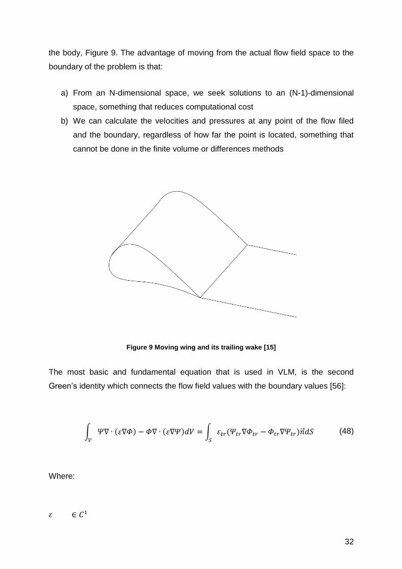
the body, Figure 9. The advantage of moving from the actual flow field space to the

boundary of the problem is that:

a) From an N-dimensional space, we seek solutions to an (N-1)-dimensional

space, something that reduces computational cost

b) We can calculate the velocities and pressures at any point of the flow filed

and the boundary, regardless of how far the point is located, something that

cannot be done in the finite volume or differences methods

Figure 9 Moving wing and its trailing wake [15]

The most basic and fundamental equation that is used in VLM, is the second

Green’s identity which connects the flow field values with the boundary values [56]:

∫ 𝛹∇ ∙ (𝜀∇𝛷) − 𝛷∇ ∙ (𝜀∇𝛹)𝑑𝑉 = ∫ 𝜀𝑡𝑟(𝛹𝑡𝑟∇𝛷𝑡𝑟 − 𝛷𝑡𝑟∇𝛹𝑡𝑟)��𝑑𝑆𝑆𝑉

(48)

Where:

𝜀 ∈ 𝐶1

33

𝛹, 𝛷 ∈ 𝐶2

𝑆 is the boundary of our domain (i.e. our support)

𝑉 is the flow filed domain

From the above equation, we can extract the so-called “Representation Theorems”,

which are used to model our problem [39]:

𝜑(��) = −1

4𝜋∫

𝜎

𝑟𝑆

𝑑𝑆 +1

4𝜋∫

�� ∙ 𝑟 ∙ 𝜇

𝑟3𝑆

𝑑𝑆 (49)

∇𝜑(��) =1

4𝜋∫ 𝜎

𝑆

𝑟

𝑟3𝑑𝑆 +

1

4𝜋∫ ��

𝑆

×𝑟

𝑟3𝑑𝑆 (50)

Equation (48) calculates the potential at any point in the flow field and on the body,

while equation (49) calculates the induced velocities from the flow field potential. In

addition, equation (49) is used in the no-entrance boundary condition and is the one

that we are going to be concerned with.

In the above equations:

𝜇 ≡ 𝜑+ − 𝜑− is the perturbation potential jump on A of the boundary

𝜑+, 𝜑− are the perturbation potentials on a point A of the

boundary

34

𝜎 ≡ ��({∇Φ}𝑡𝑟+ − {∇Φ}𝑡𝑟

− ) called surface source intensity

�� is the normal unit vector to a point A on the boundary S

{∇Φ}𝑡𝑟+ , {∇Φ}𝑡𝑟

− are the perturbation velocities on a point A of the

boundary

𝑟 is the distance of the control point �� from a point �� on

S

�� ≡ �� × ({∇Φ}𝑡𝑟+ − {∇Φ}𝑡𝑟

− ) called surface vorticity intensity

The superscripts (+,-) suggest that the parameter refers to a point A on the boundary

S, but with the additional fact that the surface S has been modeled as a surface of

discontinuity [39]. A surface of discontinuity is a two-sided surface where each point

A is denoted by 𝐴+, 𝐴−. The subscript (tr) refers to the trace of a function at a point A

on the boundary and is defined as the limit of the function as it is approaching the

point A.

In our case of study, we examine the movement of a thin rigid wing, which can be

approximated by a mean camber surface, Figure 10. The camber of a section foil is

defined as the mean line from the upper and lower side of the airfoil. A thin airfoil is

defined as an airfoil that has a small thickness compared to its chord.

35

Figure 10 Mean camber line of a wing's section [15]

Since, we are dealing with slender wings it is safe to assume that the outline of the

wing lies on the mean camber surface 𝑆𝑐 and consequently in the limiting case this

surface can be approximated by a surface of discontinuity. This means that we can

distinguish between an upper 𝑆𝑐+ and lower 𝑆𝑐

− side of the camber surface. In the

limiting case where the thickness of the wing tends to zero we have the following

boundary conditions [39]:

�� ∙({∇Φ}𝑡𝑟

+ − {∇Φ}𝑡𝑟− )

2= ∆�� ∙ (𝑉𝐴

− 𝑉∞ ) (51)

�� ∙({∇Φ}𝑡𝑟

+ + {∇Φ}𝑡𝑟− )

2= �� ∙ (𝑉𝐴

− 𝑉∞ ) (52)

In the above equations, Figure 10:

∆�� = 𝑛+ − �� = 𝑛− + ��

A+ ��

A

A- 𝑛−

𝑛+

36

𝑉𝐴, 𝑉∞

are the velocity of point A and the undisturbed velocity at infinity respectively

In case, where the wing has no thickness ∆�� = 0 that is the reason why we say that

equation (51) defines the thickness problem, while equation (52) the camber

problem. In our case where the wing is considered with zero thickness ∆�� = 0 and

consequently from equation (51) we deduce that 𝜎 = 0 on the wing. The kinematic

condition3 also lead to 𝜎 = 0, on the wake. This simplifies equation (49) to:

∇𝜑(��) =1

4𝜋∫ ��

𝑆

×𝑟

𝑟3𝑑𝑆 (53)

As can be seen equation (53) refers to a specific point in the flow field or the

boundary. By taking advantage of the no-entrance boundary condition and by

defining a certain number of discrete points on the body and the wake we can create

an integral equation which in the discretized form results in a system of linear

equations and could be solved for the unknowns. In our case the unknowns would

be the circulation 𝛤 on the wing and on the first strip of the wake, which is in contact

with the wing, this strip is called a “Kutta” strip, Figure 11. The right-hand side of the

system comprises from the resultant velocity at each of the discrete points of the

body on the normal direction and the normal velocities induced by the wake at these

points, without the Kutta strip. Hence, the no entrance boundary condition can be

written as:

∇𝜑(��) ∙ �� = ��(��) ∙ �� (54)

3 The kinematic condition stems from the physical consideration, that the free shear layer cannot form

two distinct surfaces and consequently at any point A of the layer ��+ ∙ {∇Φ}𝑡𝑟+ (A) = ��− ∙ {∇Φ}𝑡𝑟

− (𝐴).

37

Figure 11 Definition of the Kutta strip

Following the above discussion equation (53) can be re-written as:

(1

4𝜋∫ ��

𝑜𝑛 𝑤𝑖𝑛𝑔

×𝑟

𝑟3𝑑𝑆 +

1

4𝜋∫ ��

𝑜𝑛 𝑘𝑢𝑡𝑡𝑎 𝑠𝑡𝑟𝑖𝑝

×𝑟

𝑟3𝑑𝑆) ∙ ��

= (��(��) −1

4𝜋∫ ��

𝑜𝑛 𝑤𝑎𝑘𝑒

×𝑟

𝑟3𝑑𝑆) ∙ ��

(55)

Grid discretization

As already described at the beginning of previous section, in order to numerically

calculate the forces, velocities, pressures on the body, we discretize the geometry of

our problem, by using panel elements. Four types of panels would be needed for

describing our problem:

38

1. Geometry panels

2. Vortex panels

3. Wake panels

4. Kutta strip panels

Both the geometry and vortex panels refer on the wing, however in order to avoid

numerical instabilities we are forced to distinguish between them, Figure 12. The

wake is also discretized by panel elements, however a distinction of two regions is

required here too. The first strip of the wake is the ‘Kutta’ strip and is discretized by

the Kutta strip panels, while the rest of the wake is discretized by the wake panels,

Figure 13.

Figure 12 Definition of geometry and vortex panel

39

Figure 13 Distinction between wake panels and kutta panels

The geometry panels are generated by a Geometry Preprocessor Program (GPP),

where the span and chord lengths are given as input, together with the number of

panels, both span-wise and chord-wise. The motion of the body is given by a Motion

Preprocessor Program (MPP) where all the characteristics of the motion are given.

The output of GPP and MPP is inserted as input in the VLMU program, which in–turn

performs all the necessary steps to find the forces, velocities and pressures on the

body and the velocities on the wake.

Each of the rest of the panels comprise of four corner nodes, which are numbered as

in Figure 14. In the vortex and Kutta strip panels a collocation point is defined (cf.

Chapter 2). On the collocation points of the vortex panels we implement the no-

entrance boundary condition, while on the Kutta strip points we implement the Kutta

condition. The Kutta condition is basically a physical consideration and is based on

the observation that the flow leaving the trailing edge should be of finite value. In

addition, on the common boundary of the vortex panels we define a control point,

which is used for the calculation of forces and pressures.

40

Figure 14 Numbering of corner nodes in each element [15]

Finally, in the VLM we assume a constant piece-wise dipole distribution 𝜇. By taking

into account the relation between dipole and vortex intensity [39]:

�� = �� × ∇𝜇 (56)

we conclude that in each panel a zero vortex distribution exists. However, the

integral ∫ �� ×𝑟

𝑟3 𝑑𝑆 can be written as [39]:

∫ ��𝑝𝑎𝑛𝑒𝑙

×𝑟

𝑟3𝑑𝑆 = ∫ 𝛤𝑀𝑁 ∙

𝑑𝑙 × 𝑟

𝑟3𝐿

(57)

Equation (56) can be re-written as:

41

∫ ��𝑝𝑎𝑛𝑒𝑙

×𝑟

𝑟3𝑑𝑆

= 𝛤𝑀𝑁 (∫𝑑𝑙

13 × 𝑟𝑐𝑝𝐼𝐽

𝑟313

+ ∫𝑑𝑙


𝑟334

+ ∫𝑑𝑙


𝑟342

+ ∫𝑑𝑙


𝑟321

)

(58)

In the above equation 𝛤𝑀𝑁 is the MN panel’s circulation and we define:

𝐺𝑀𝑁𝐼𝐽 = (∫

𝑑𝑙13 × 𝑟𝑐𝑝

𝐼𝐽

𝑟313

+ ∫𝑑𝑙


𝑟334

+ ∫𝑑𝑙


𝑟342

+ ∫𝑑𝑙


𝑟321

) (59)

The integrals ∫𝑑𝑙𝐾𝐿×𝑟𝑐𝑝

𝐼𝐽

𝑟3𝐾𝐿 in equation (57) are called the induction factors of the line

segment KL (belongs to the MN panel) to the collocation point of the IJ panel.

Linear system of equations

Suppose that we have partitioned our grid with 𝑁𝑌 span-wise panels and 𝑁𝑋 chord-

wise panels, the sum of the collocation points is 𝑁𝑁 = 𝑁𝑌 ∙ 𝑁𝑋. The number of the

Kutta strip and wake panels in the span-wise direction is also 𝑁𝑌. Each panel has a

constant circulation 𝛤𝐼𝐽, where:

a) 𝐼 = 1, … , 𝑁𝑌 and 𝐽 = 1, … , 𝑁𝑋, for the vortex panels

b) 𝐼 = 1, … , 𝑁𝑌 and 𝐽 = 𝑁𝑋 + 1, for the Kutta strip panels

c) 𝐼 = 1, … , 𝑁𝑌 and 𝐽 = 𝑁𝑋 + 2, … , (𝑁𝑋 + 2 + 𝑖𝑡𝑠), for the wake panels, 𝑖𝑡𝑠 =

0, … , 𝑛𝑡𝑠

42

The index 𝑖𝑡𝑠 refers to the time-step that the code is at the moment and the index 𝑛𝑡𝑠

to the total number of time-steps the VLWU4 will calculate. The reason for the

presence of 𝑖𝑡𝑠 in the number of wake panels is that the wake is generated

dynamically. In order to explain the previous statement, let us imagine that we are at

a time-step 𝑖𝑡𝑠 = 𝑖0. At this time-step the algorithm has already calculated the 𝛤𝐼𝐽 on

the body and the Kutta strip at the end of the previous time-step and has already

calculated the position and 𝛤𝐼𝐽 of the wake. By solving the linear system of equations

at this time-step the algorithm calculates the:

1. new 𝛤𝐼𝐽 on the body

2. moves the body to its new position

3. new 𝛤𝐼𝐽 on the new Kutta strip

4. defines the new Kutta strip position that should be always in contact with the

trailing edge line

5. the Kutta strip at the previous time-step becomes a part of the wake

6. deforms the wake panels according to the perturbation velocities induced on

the wake panels

7. VLWU is ready to solve for next time-step

From the above point 5) is the reason why 𝑖𝑡𝑠 is present on b). Hence, at each time

the number of panels in the wake increases by 𝑁𝑌.

From the above considerations equation (54) for each collocation point, becomes:

( ∑ ∑ 𝛤𝑀𝑁 ∙ 𝐺𝑀𝑁𝐼𝐽

𝑁𝑋

𝑁=1

𝑁𝑌

𝑀=1

+ ∑ ∑ 𝛤𝑀𝑁 ∙ 𝐺𝑀𝑁𝐼𝐽

𝑁𝑋+1

𝑁=𝑁𝑋+1

𝑁𝑌

𝑀=1

) ∙��

4𝜋

= (��(��𝐼𝐽) −1

4𝜋∑ ∑ 𝛤𝑀𝑁 ∙ 𝐺𝑀𝑁

𝐼𝐽

𝑁𝑋+2+𝑖𝑡𝑠

𝑁=𝑁𝑋+2

𝑁𝑌

𝑀=1

) ∙ �� (60)

4 Vortex Lattice Wing Unsteady (VLWU)

43

The above equation forms a system of 𝑁𝑁 = 𝑁𝑌 ∙ 𝑁𝑋 equations with 𝑁𝑌 ∙ (𝑁𝑋 + 1)

unknowns. The final equation to complete the system will be given by the Kutta

condition (cf. Chapter 2). As can be seen from equation (59), the unknowns are

the 𝛤𝑀𝑁 of the left-hand side only, since the 𝛤𝑀𝑁 of the wake (right-hand side) have

been calculated in the previous time-step and consequently are already known.

44

Chapter 2 Describing the Method

In this chapter, we are going to describe the equations used in our modelling. We are

also going to define the notion of the Kutta condition in a more detailed manner and

we are going to calculate the pressures and forces acting on the wing. All equations

are going to be formulated for an IFoR.

2.1 Equations used in our modeling

The equations that describe the problem of the unsteady flow around a rectangular

wing with zero thickness, are:

1. The no-entrance condition5:

( ��∞(x, y, z, t) + ��(𝑥) + 𝑉′

𝐴𝑃 + ∇𝜑𝑤𝑎𝑘𝑒) ∙ �� = ∇𝜑𝑤𝑖𝑛𝑔 & 𝑘𝑢𝑡𝑡𝑎 𝑠𝑡𝑟𝑖𝑝 ∙ �� (61)

Where:

��∞(x, y, z, t) = 𝑉𝑡 (x, y, z, t) + ℎ(𝑡) (62)

Where:

5 The capital case unit vectors 𝐼, 𝐽, �� will refer to the OXYZ IFoR, while the lower case unit

vectors 𝑖, 𝑗, �� to the O’xyz NIFoR, unless otherwise stated.

45

��∞ is the velocity at infinity

∇𝜑𝑤𝑎𝑘𝑒 is the perturbation velocity induced by the wake

�� is the normal to a point on the wing, with respect to a body-fixed frame

of reference.

∇𝜑 is the perturbation velocity potential

𝑉𝑡 is the velocity of advance of the wing

𝑉′𝐴𝑃 is given by equation (47)

ℎ(𝑡) is the velocity as produced by the heaving motion of the wing

ℎ(𝑡) = ℎ0 ∙ cos 2𝜋 ∙ 𝑓 ∙ 𝑡

ℎ0 is the heaving amplitude

𝑓 is the frequency of the oscillatory heaving motion

��(𝑥) sinusoidal gust with respect to IFoR

46

In order to have a unique solution to our problem we need to apply the Kutta

condition at the trailing edge of the wing:

𝑝𝑢 = 𝑝𝑙 (63)

Equation (63) states that as you approach the trailing edge from the suction (upper)

and the pressure (lower) side the pressures in both sides become equal. It can be

shown [39] that the above equation can be written as:

𝜕( 𝜑𝑢 − 𝜑𝑙)

𝜕𝑡+ (�� × �� + 𝜎 ∙ ��)(⟨��⟩ + ��) = 0 (64)

Where:

𝜑𝑢, 𝜑𝑙 is the perturbation potential on the upper and lower side of the trailing edge

�� = (𝛾1, 𝛾2, 0) is the surface vorticity intensity

𝜎 ≡ ��( ∇𝜑𝑢 − ∇𝜑𝑙) is called surface source intensity

�� is the normal at a point of the wake surface

⟨��⟩ ≡ 0.5(∇𝜑𝑢 + ∇φ𝑙) is called the mean fluid perturbation velocity

It can be shown [39] that in equation (64) 𝜎 = 0 on the trailing edge. We also apply

the dynamic condition on every point of the wake [39]:

47

𝑝+ = 𝑝− (65)

Where 𝑝+, 𝑝− are the pressures on the upper and lower part of the wake surface at

the same point.

Equation (65) can be written in the form of equation (64):

𝜕(𝜑+ − 𝜑−)

𝜕𝑡− (�� × �� + 𝜎 ∙ ��)(⟨��⟩ + ��∞) = 0 (66)

It can also be shown [39] that in equation (66) 𝜎 = 0 on the every point of the wake

(dynamic condition).

2.2 Modeling of vorticity

In this section we describe in more detail the modeling and geometry of the panels,

used in our method. We model the vorticity on the wing and the wake by using

rectilinear panels (vortex panels), where each panel is assigned with a constant

vorticity strength 𝛤𝑖𝑗. In Figure 15 we can see the arrangement of the panels both on

the wing and on the wake. NY is the total number of vortex panels in the y–direction,

NX is the total number of vortex panels in the x-direction and Nw is the number of

panels in the wake in the x-direction at a certain time-step (changes with each time-

step).

48

Figure 15 Arrangement of vorticity on panels

The Vortex Lattice Method is an extension of the “Lumped-Vortex Method”, in which

the vortex strengths are placed at the quarter length of each panel in the chord-wise

direction, while the boundary conditions are satisfied on the collocation points (three

quarters length of each panel in the chord-wise direction) [22]. In our modeling the 𝑖, 𝑗

indices describe the vortex strength (i.e. control points), while the 𝑘, 𝑙 indices

describe the collocation points.

At this stage we need to make a distinction between a geometric/body panel and a

vortex panel. The first refers to discretizing the geometry of the wing in rectilinear

panels, where each geometric panel has breadth 𝛥𝑌𝑔 =𝑠𝑝𝑎𝑛

𝑁𝑌⁄ and length 𝛥𝑋𝑔 =

𝑐ℎ𝑜𝑟𝑑𝑁𝑋⁄ . Due to numerical instabilities, each vortex panel has breadth 𝛥𝑌𝑣 =

𝑠𝑝𝑎𝑛(𝑁𝑌 + 0.5)⁄ and length 𝛥𝑋𝑣 = 𝑐ℎ𝑜𝑟𝑑

𝑁𝑋⁄ . In addition, each vortex panel is

placed a quarter of 𝛥𝑋𝑔 behind the respective geometric panel.

Each vortex panel has four corners (cf. Figure 14), the coordinates for each vortex

panel, in the body fixed frame of reference, are:

49

𝑌1(𝑖, 𝑗) = 𝑌2(𝑖, 𝑗) =

𝛥𝑌𝑔4

⁄ + (𝑖 − 1) ∙ 𝛥𝑌𝑔 + 𝑌𝑂′ (67)

𝑌3(𝑖, 𝑗) = 𝑌4(𝑖, 𝑗) =

𝛥𝑌𝑔4

⁄ + 𝑖 ∙ 𝛥𝑌𝑔 + 𝑌𝑂′ (68)

𝑋1(𝑖, 𝑗) = 𝑋3(𝑖, 𝑗) =

𝛥𝑋𝑔4

⁄ + (𝑖 − 1) ∙ 𝛥𝑋𝑔 + 𝑋𝑂′ (69)

𝑋2(𝑖, 𝑗) = 𝑋4(𝑖, 𝑗) =

𝛥𝑋𝑔4

⁄ + 𝑖 ∙ 𝛥𝑋𝑔 + 𝑋𝑂′ (70)

Where 𝑌𝑂′ , 𝑋𝑂′ are the Y, X-coordinates of the origin of the NIFoR from the IFoR.

In order to solve our problem, we need to solve the following equations:

a) The no-entrance boundary condition at the 𝑁𝑌 ∙ 𝑁𝑋 collocation points

b) The pressure type Kutta condition at the 𝑁𝑌 collocation points, which lie on

the Kutta strip

Hence, the total number of equations that we need to solve are:

𝑁𝐸𝑄𝑆 = 𝑁𝑌(𝑁𝑋 + 1) (71)

Two types of indices are used in the code 𝑖𝑗 and 𝑘𝑙. The former are used in order to

tag the unknown vorticity of, Figure 16:

a) The wing vortex panels

b) The wake’s first layer vortex panels (i.e. Kutta strip)

50

The latter are used in order to tag the position of the collocation points:

a) On the wing

b) On the wake

Figure 16 Numbering of collocation points

The relation between the 𝑖𝑗 index and the 𝑖, 𝑗 indices are:

𝑖𝑗 = (𝑖 − 1)(𝑁𝑋 + 1) + 𝑗 (72)

The relation between the 𝑘𝑙 index and the 𝑘, 𝑙 indices are:

a) On the wing panels

𝑘𝑙 = (𝑘 − 1)𝑁𝑋 + 𝑙 (73)

51

b) On the wake panels

𝑘𝑙 = 𝑁𝑌 ∙ 𝑁𝑋 + 𝑙 (74)

Before moving any further we need to point out that equations (67)÷(70) refer to a

body fixed frame of reference (i.e. 𝑂′𝑥𝑦𝑧). Since, we are going to solve our problem

for an inertial frame of reference we need to transform these equations.

The transformation from 𝑂′𝑥𝑦𝑧 to 𝑂′𝑋′𝑌′𝑍′ is:

[𝑋′𝑌′𝑍′

] = [cos 𝜃(𝑡) 0 sin 𝜃(𝑡)

0 1 0− sin 𝜃(𝑡) 0 cos 𝜃(𝑡)

] [𝑥𝑦𝑧

] + [0.25𝑐

00

] (75)

The transformation from 𝑂′𝑋′𝑌′𝑍′ to 𝑂𝑋𝑌𝑍 is:

[𝑋𝑌𝑍

] = [𝑋′𝑌′𝑍′

] + [−‖𝑉𝑡 ‖ ∙ 𝛥𝑡

0ℎ(𝑡)

] (76)

By combining (75) and (76) we can write the transformation from 𝑂′𝑥𝑦𝑧 to 𝑂𝑋𝑌𝑍 :

[𝑋𝑌𝑍


0 1 0− sin 𝜃(𝑡) 0 cos 𝜃(𝑡)

] [𝑥𝑦0

] + [−‖𝑉𝑡 ‖ ∙ 𝛥𝑡 + 0.25𝑐

0ℎ(𝑡)

] (77)

Where we have used the fact that in the 𝑂′𝑥𝑦𝑧 frame the z-coordinate of the wing is

always zero. The above transformations are used in our code in order to transform

from the body-fixed frame of reference to the IFoR.

52

2.3 Time discretization

A very significant parameter, for computing as accurate as possible the forces acting

on the wing and the velocities of the fluid, is the discretization of time. Time is of

great importance since too sparse time-steps would lead to loss of valuable

information (i.e. not good description of the problem), too many time-steps would

cost in computational effort. This means that we need to specify the time-steps

based on some criteria.

For motions that have a “periodic” nature, a certain number of time-steps in a

period 𝑇 is needed to describe, within a good approximation, the unsteady velocity of

the fluid. In our case of study the motion of the wing is not periodic, due to the

presence of the perturbation velocity. However, since the magnitude of the

perturbation velocity can be considered small compared to the other velocity

components, we can assume a periodic motion.

Hence, a good time-step resolution, for periodic motions, can be calculated by [45]:

𝛥𝑡 =

𝑇

𝑁𝑇𝑆𝑃𝑃 (78)

Where 𝑁𝑇𝑆𝑃𝑃 is the number of time-steps per period.

Finally, we need to decide the total number of time-steps 𝑁𝐷𝑇𝐼𝑀 required to

describe accurately the periodic motion. This number can be given by [45]:

𝑁𝐷𝑇𝐼𝑀 =

𝑁𝑃𝐸𝑅𝐼𝑂𝐷 ∙ 𝑇

𝛥𝑡= 𝑁𝑃𝐸𝑅𝐼𝑂𝐷 ∙ 𝑁𝑇𝑆𝑃𝑃 (79)

Where 𝑁𝑃𝐸𝑅𝐼𝑂𝐷 is the required number of periods to describe as accurate as

possible the motion.

53

The way of selecting a specific 𝑁𝐷𝑇𝐼𝑀, 𝑁𝑃𝐸𝑅𝐼𝑂𝐷 and 𝑁𝑇𝑆𝑃𝑃 depends on the

specific phenomenon and the dimensionless parameters that describe it. This means

that these parameters are heuristically chosen most of the time. It can be seen from

equations (78) and (79) that the greater the 𝑇 (i.e. the smaller the frequency 𝑓) the

more 𝑁𝑇𝑆𝑃𝑃 and 𝑁𝑃𝐸𝑅𝐼𝑂𝐷 are needed to describe the phenomenon with the same

resolution.

2.4 Wake panels modeling

Another important decision that we need to take is the wake panels’ length and

consequently the vortex panel’s length. It can be shown [39] that due to the Kutta

condition, the span-wise surface vorticity intensity produced at the trailing edge is

transferred on the wake with a rate of 𝑑𝛤

𝑑𝑡 .

Each wake panel is only moving due to the perturbation velocities and not due to the

velocity at infinity. This type of wake formulation, where the shear layer is deformed

by the perturbed velocities is called a free shear layer formulation. In the case where

the wake is not deformed by the perturbed velocities, the position of each panel

stays freeze in space at any instant, this type of formulation is called a frozen shear

layer formulation. The length of each wake panel will be given by 𝐷𝑊𝑥 = 𝑉∞ ∙ 𝑑𝑡,

where 𝑑𝑡 has been calculated by the time discretization.

The kinematic condition on the shear layer basically states that the normal velocities

of the fluid on a point “A” of the wake should be equal in direction and size on both

sided of the wake at “A”. This condition, however, states nothing about the tangential

velocities on the wake. The tangential velocities could vary for the same point on the

upper and lower surface, something that introduces a velocity discontinuity jump

which is not observed in reality. In addition, the roll-up of the wake at the wing tips

will inevitably produce infinite velocities to itself. This introduces another type of

singularity at the shear layer. Finally, the fact that we have modeled the wake of the

real problem with a surface of zero-thickness leads inevitably to the so-called Kelvin-

Helmholtz Instabilities (KHI). The KHI are small scale instabilities and lead to a

chaotic behavior of the shear layer, where any attempt to describe the deformation of

54

the layer by the induced velocities on the wake by itself would lead to a

discontinuous deformation of the wake. This fact can easily be seen by the singular

nature of the solutions of our problem, where any attempt on calculating the induced

factors from equation (59), would lead at some point to the zeroing of the

denominator and will cause a singularity at this point.

In nature, however, we do not observe any singularities and the reason for this is

that viscosity suppresses these instabilities. Thus, in order to suppress all the above

mentioned singularities we need to introduce a virtual viscosity. This is done by

expressing the velocity induced by a vortex filament by the “Lamb-Oseen” vortices,

which are exact solutions of the Navier-Stokes equations [57]. We use the proposed

method given by Politis [38], where the induced azimuthal velocity will be given by:

𝑢𝜃 =

𝛤

2𝜋 ∙ 𝑟∙ (1 − 𝑒−𝑐∙(

𝑟𝑅

)2

) (80)

Equation (80) and equation (57) have similarities. In addition, equation (80) mollifies

any singularities at 𝑟 = 0, this is why we call the factor (1 − 𝑒−𝑐∙(𝑟

𝑅)

2

) a mollifier. The

above equation replaces a vortex filament with a viscous vortex core of finite

diameter. In addition, parameters “c”, “R” control the diameter of the viscous vortex

core. In Politis [38] the value of the parameter is replaced by 0.69314718 , which

leaves only as a controlling parameter, the parameter “R”. “R” is calculated as a

percentage of the span of the wing, as we increase “R” the shear layer approaches

the “prescribed” wake model method. As we decrease “R” the shear layer

approached to the chaotic behavior of the wake. In order to represent the wake

deformation as accurate as possible “R” should neither be too large not too small.

The value of “R” is case dependent and could vary from 0.5% to 15% [38].

55

2.5 The no-entrance boundary condition

The no-entrance boundary condition that we implement on the collocation points is

comprised by three parts:

a) The normal component of the velocity at infinity on the wing’s surface at the

collocation point 𝑉𝑎 = −𝑉∞ ∙ sin 𝑎(𝑡),

b) The normal component of the perturbation velocity 𝑉𝑤 due to the wake panels,

without the Kutta strip, 𝑉𝑤𝑎𝑘𝑒 = −∇𝜑𝑤𝑎𝑘𝑒 ∙ ��

c) The normal component of the sinusoidal gust background field, 𝑉𝑔𝑢𝑠𝑡 = w(x) ∙

��

d) The velocity component of the pitching motion on the wing, with respect to the

pitching axis

In our modeling, as already explained in section 1.3.3 the no entrance boundary

condition forms the right-hand side (RHS) of our system of equations that we are

going to solve. Hence, the no-entrance boundary condition is given by:

𝑅𝐻𝑆 = 𝑉𝑎 + 𝑉𝑤𝑎𝑘𝑒 + 𝑉𝑔𝑢𝑠𝑡 + 𝑉′𝐴𝑃 (81)

The number of the above equations are 𝑁𝑋 ∙ 𝑁𝑌 and consequently 𝑁𝑌 more

equations are need in order to complete our system. These will be given by the Kutta

condition (cf. section 2.7).

2.6 Calculation of pressure difference and forces

Let’s focus on two adjacent vortex panels 𝑖, 𝑗 and 𝑖, 𝑗 − 1, with 𝑗 ≥ 16. It can be shown

that the connection between the vortex strengths of the two panels is:

6 A vortex panel with 𝑗 = 0 is defined with zero vorticity 𝛤𝑖,0

56

𝛤′𝑖,𝑗 = 𝛤𝑖,𝑗 − 𝛤𝑖,𝑗−1 (82)

Where 𝛤′𝑖,𝑗 is the vortex strength of the common boundary between the two panels.

Notice that the control point on which we assign the 𝛤′𝑖,𝑗 is in the middle of the line

joining the two control points 𝑖, 𝑗 and 𝑖, 𝑗 − 1 Figure 17.

Figure 17 Vorticity assigned on a control point

The circulation of the panel 𝑖, 𝑗 around a path ‘c’ that intersects the vortex panel at

the control point, can be found by:

∮ ��𝑑𝑙𝐶

= 𝜑𝑖,𝑗𝑢 − 𝜑𝑖,𝑗

𝑙 = 𝛤𝑖,𝑗 (83)

The same equation can be written for the common line of intersection of the two

panels 𝑖, 𝑗 and 𝑖, 𝑗 − 1:

57

∮ ��𝑑𝑙𝐶′

= 𝜑′𝑖,𝑗𝑢 − 𝜑′𝑖,𝑗

𝑙 = 𝛤′𝑖,𝑗 (84)

In order to draw a connection between equation (83) and (84) we perform:

i. A Taylor expansion for 𝜑′𝑖,𝑗𝑢 around 𝜑𝑖,𝑗

𝑢 of first order approximation in the x-

direction:

𝜑′𝑖,𝑗𝑢 = 𝜑𝑖,𝑗

𝑢 +𝜕 𝜑𝑖,𝑗

𝑢

𝜕𝑥∙ 𝑑𝑥 (85)

ii. A Taylor expansion for 𝜑′𝑖,𝑗𝑢 around 𝜑𝑖,𝑗−1

𝑢 of first order approximation in the x-

direction:

𝜑′𝑖,𝑗

𝑢 = 𝜑𝑖,𝑗−1𝑢 −

𝜕 𝜑𝑖,𝑗−1𝑢

𝜕𝑥∙ 𝑑𝑥

(86)

If we add equations (85) and (86) and assume that 𝜕 𝜑𝑖,𝑗−1

𝑢

𝜕𝑥=

𝜕 𝜑𝑖,𝑗𝑢

𝜕𝑥 we end up with:

𝜑′𝑖,𝑗𝑢 =

𝜑𝑖,𝑗𝑢 + 𝜑𝑖,𝑗−1

𝑢

2 (87)

By applying the same notion for 𝜑′𝑖,𝑗𝑙 we end up in a similar equation:

58

𝜑′𝑖,𝑗𝑙 =

𝜑𝑖,𝑗𝑙 + 𝜑𝑖,𝑗−1

𝑙

2 (88)

Equation (84) becomes:

∮ ��𝑑𝑙

𝐶′

=( 𝜑𝑖,𝑗

𝑙 + 𝜑𝑖,𝑗−1𝑢 ) − ( 𝜑𝑖,𝑗

𝑙 + 𝜑𝑖,𝑗−1𝑙 )

2=

𝛤𝑖,𝑗 + 𝛤𝑖,𝑗−1

2

(89)

Let’s take a rectangle around the common boundary of the vortex panels 𝑖, 𝑗

and 𝑖, 𝑗 − 1, with area 𝛥𝑥 ∙ 𝛥𝑦. This panel is defined to have as center the point

where 𝛤′𝑖,𝑗 is placed. The force, as measured on the body-fixed frame of

reference, developed by this area is defined as [39]:

𝐹𝑖,𝑗 = 𝜌 ∙ (��∞ × 𝛤′𝑖,𝑗

∙𝛥𝑦

cos(𝑇𝐴𝑃𝐴𝑁𝐺)+ ��

𝜕(𝜑′𝑖,𝑗𝑢 − 𝜑′𝑖,𝑗

𝑙 )

𝜕𝑡𝛥𝑥 ∙ 𝛥𝑦) (90)

Where 𝑇𝐴𝑃𝐴𝑁𝐺 is the angle of Figure 18. In order to evaluate the components of 𝐹𝑖,𝑗

in the x and z-directions we have:

𝛤′𝑖,𝑗 = (sin(𝑇𝐴𝑃𝐴𝑁𝐺) ∙ 𝑖 + cos(𝑇𝐴𝑃𝐴𝑁𝐺) ∙ 𝑗) ∙ 𝛤′𝑖,𝑗 (91)

59

Figure 18 Definition of angle of taper

Hence, we have:

��∞ × 𝛤′𝑖,𝑗

= |

𝑖 𝑗 ��

𝑉∞(x, y, z, t) ∙ cos(𝑎(𝑡)) 0 𝑉∞(x, y, z, t) ∙ sin(𝑎(𝑡))

sin(𝑇𝐴𝑃𝐴𝑁𝐺) ∙ 𝛤′𝑖,𝑗 cos(𝑇𝐴𝑃𝐴𝑁𝐺) ∙ 𝛤′

𝑖,𝑗 0

|

= −cos(𝑇𝐴𝑃𝐴𝑁𝐺) ∙ 𝛤′𝑖,𝑗 ∙∙ 𝑖 + sin(𝑇𝐴𝑃𝐴𝑁𝐺) ∙ 𝛤′

𝑖,𝑗

∙ (𝑉∞(x, y, z, t) ∙ sin(𝑎(𝑡))) ∙ 𝑗 + cos(𝑇𝐴𝑃𝐴𝑁𝐺) ∙ 𝛤′𝑖,𝑗 ∙ (𝑉∞(x, y, z, t) ∙ cos(𝑎(𝑡))) ∙ ��

(92)

Hence, equation (90) becomes in the z-direction:

𝐹𝑧 𝑖,𝑗 = 𝜌 ∙ ( 𝛤′

𝑖,𝑗 ∙ (𝑉∞(x, y, z, t) ∙ cos(𝑎(𝑡))) ∙ 𝛥𝑦 +𝜕(𝜑′𝑖,𝑗

𝑢 − 𝜑′𝑖,𝑗𝑙 )

𝜕𝑡𝛥𝑥 ∙ 𝛥𝑦)

(93)

60

In the x-direction:

𝐹𝑥 𝑖,𝑗 = −𝛥𝑦∙ 𝛤′𝑖,𝑗 ∙ (𝑉∞(x, y, z, t) ∙ sin(𝑎(𝑡))) ∙ 𝜌 (94)

In the y-direction:

𝐹𝑦 𝑖,𝑗 = tan(𝑇𝐴𝑃𝐴𝑁𝐺) ∙ 𝛤′𝑖,𝑗 ∙ (𝑉∞(x, y, z, t) ∙ sin(𝑎(𝑡))) ∙ 𝛥𝑦 ∙ 𝜌 (95)

However, equations (93), (94) and (95) refer to the frame of reference 𝑂′𝑥𝑦𝑧. In

order to transform these equations to the 𝑂𝑋𝑌𝑍 frame of reference we need to

multiply 𝐹𝑖,𝑗 with the rotation matrix:

𝐹𝑖,𝑗

𝑂𝑋𝑌𝑍= [

𝐹𝑋 𝑖,𝑗

𝐹𝑌 𝑖,𝑗

𝐹𝑍 𝑖,𝑗


0 1 0− sin 𝜃(𝑡) 0 cos 𝜃(𝑡)

] [

𝐹𝑥 𝑖,𝑗

𝐹𝑦 𝑖,𝑗

𝐹𝑧 𝑖,𝑗

] (96)

The lift and drag force developed in each panel can be evaluated by:

𝐿𝑖𝑓𝑡𝑖,𝑗 = 𝑙 ∙ 𝐹𝑖,𝑗

𝑂𝑋𝑌𝑍 (97)

61

𝐷𝑟𝑎𝑔𝑖,𝑗 = 𝑡 ∙ 𝐹𝑖,𝑗

𝑂𝑋𝑌𝑍 (98)

Where:

𝑙 = − sin 𝜑(𝑡) ∙ 𝛪 + cos 𝜑(𝑡) ∙ �� (99)

𝑡 = cos 𝜑(𝑡) ∙ 𝛪 + sin 𝜑(𝑡) ∙ �� (100)

Are the normal and tangential vectors, with respect to the angle of attack, as

measured in the 𝑂𝑋𝑌𝑍 frame of reference. Where the angle 𝜑(𝑡) = 𝑎(𝑡) + 𝜃(𝑡).

Hence, we conclude that:

𝐿𝑖𝑓𝑡𝑖,𝑗 = −𝐹𝑋 𝑖,𝑗 ∙ sin 𝜑(𝑡) + 𝐹𝑍 𝑖,𝑗 ∙ cos 𝜑(𝑡) (101)

𝐷𝑟𝑎𝑔𝑖,𝑗 = 𝐹𝑋 𝑖,𝑗 ∙ cos 𝜑(𝑡) + 𝐹𝑍 𝑖,𝑗 ∙ sin 𝜑(𝑡) (102)

The span-wise lift and drag are given, respectively by:

62

𝐿𝑖𝑓𝑡𝑖 = ∑ 𝐿𝑖𝑓𝑡𝑖,𝑗

𝑁𝑋

𝑗=1

(103)

𝐷𝑟𝑎𝑔𝑖 = ∑ 𝐷𝑟𝑎𝑔𝑖,𝑗

𝑁𝑋

𝑗=1

(104)

The respective lift and drag coefficients are:

𝐶𝐿𝑖=

𝐿𝑖𝑓𝑡𝑖0.5 ∙ 𝜌 ∙ 𝑉∞

2 ∙ 𝑐𝑖⁄ (105)

𝐶𝐷𝑖=

𝐷𝑟𝑎𝑔𝑖0.5 ∙ 𝜌 ∙ 𝑉∞

2 ∙ 𝑐𝑖⁄ (106)

Where 𝑐𝑖 is the chord at the span-wise position i.

The total lift and drag are given respectively by:

𝐿𝑖𝑓𝑡 = ∑ 𝐿𝑖𝑓𝑡𝑖

𝑁𝑌

𝑖=1

(107)

𝐷𝑟𝑎𝑔 = ∑ 𝐷𝑟𝑎𝑔𝑖

𝑁𝑌

𝑖=1

(108)

The respective total lift and drag coefficients are:

63

𝐶𝐿 =𝐿𝑖𝑓𝑡

0.5 ∙ 𝜌 ∙ 𝑉∞2 ∙ 𝑆⁄ (109)

𝐶𝐷 =𝐷𝑟𝑎𝑔

0.5 ∙ 𝜌 ∙ 𝑉∞2 ∙ 𝑆⁄ (110)

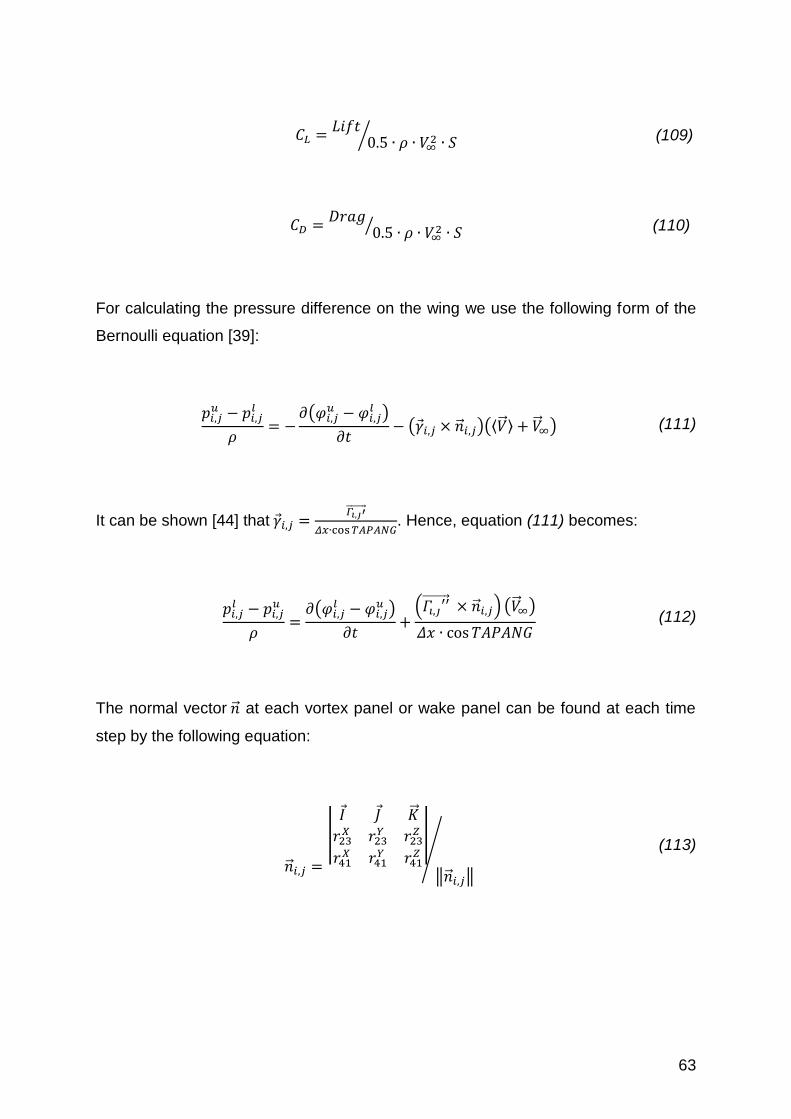
For calculating the pressure difference on the wing we use the following form of the

Bernoulli equation [39]:

𝑝𝑖,𝑗

𝑢 − 𝑝𝑖,𝑗𝑙

𝜌= −

𝜕(𝜑𝑖,𝑗𝑢 − 𝜑𝑖,𝑗

𝑙 )

𝜕𝑡− (��𝑖,𝑗 × ��𝑖,𝑗)(⟨��⟩ + ��∞) (111)

It can be shown [44] that ��𝑖,𝑗 =𝛤𝑖,𝑗′

𝛥𝑥∙cos 𝑇𝐴𝑃𝐴𝑁𝐺. Hence, equation (111) becomes:

𝑝𝑖,𝑗

𝑙 − 𝑝𝑖,𝑗𝑢

𝜌=

𝜕(𝜑𝑖,𝑗𝑙 − 𝜑𝑖,𝑗

𝑢 )

𝜕𝑡+

(𝛤𝑖,𝑗′′ × ��𝑖,𝑗) (��∞)

𝛥𝑥 ∙ cos 𝑇𝐴𝑃𝐴𝑁𝐺 (112)

The normal vector �� at each vortex panel or wake panel can be found at each time

step by the following equation:

��𝑖,𝑗 =

|𝐼 𝐽 ��

𝑟23𝑋 𝑟23

𝑌 𝑟23𝑍

𝑟41𝑋 𝑟41

𝑌 𝑟41𝑍

|

‖��𝑖,𝑗‖

⁄

(113)

64

Where:

𝑟23 = 𝑟2 − 𝑟3

𝑟41 = 𝑟4 − 𝑟1

𝑟1 , 𝑟2 , 𝑟3 , 𝑟4 are the vector positions of the corners of each panel with respect

to the 𝑂𝑋𝑌𝑍 frame of reference

The vector 𝛤𝑖,𝑗′′ is the vortex strength 𝛤𝑖,𝑗′ , with respect to the 𝑂𝑋𝑌𝑍 frame of

reference. It can be evaluated by:

𝛤𝑖,𝑗′′ = 𝛤′𝑖,𝑗 ∙ [cos 𝜃(𝑡) 0 sin 𝜃(𝑡)

0 1 0− sin 𝜃(𝑡) 0 cos 𝜃(𝑡)

] ∙ [sin 𝑇𝐴𝑃𝐴𝑁𝐺cos 𝑇𝐴𝑃𝐴𝑁𝐺

0]

We define as:

𝐴𝑖,𝑗 = {[cos 𝜃(𝑡) 0 sin 𝜃(𝑡)

0 1 0− sin 𝜃(𝑡) 0 cos 𝜃(𝑡)

] ∙ [sin 𝑇𝐴𝑃𝐴𝑁𝐺cos 𝑇𝐴𝑃𝐴𝑁𝐺

0]} × ��𝑖,𝑗

Hence, for the difference in the pressure coefficient ∆𝐶𝑝 we have from equation

(112):

∆𝐶𝑖,𝑗𝑝 =

1

0.5 ∙ 𝑉∞2 ∙

𝜕(𝜑𝑖,𝑗𝑢 − 𝜑𝑖,𝑗

𝑙 )

𝜕𝑡+

( 𝛤′𝑖,𝑗 ∙ 𝐴𝑖,𝑗)(��∞)

∙ 𝛥𝑥 ∙ cos 𝑇𝐴𝑃𝐴𝑁𝐺∙

1

10.5

∙ 𝑉∞2 (114)

65

Where:

∆𝐶𝑝 =

𝑝𝑙 − 𝑝𝑢

12 ∙ 𝜌 ∙ 𝑉∞

2

From equation (89), equation (114) becomes:

∆𝐶𝑖,𝑗𝑝 =

0.5

0.5 ∙ 𝑉∞2 ∙

𝜕(𝛤𝑖,𝑗 + 𝛤𝑖,𝑗−1)

𝜕𝑡+

( 𝛤′𝑖,𝑗 ∙ 𝐴𝑖,𝑗)(��∞)

∙ 𝛥𝑥 ∙ cos 𝑇𝐴𝑃𝐴𝑁𝐺∙

1

0.5 ∙ 𝑉∞2 (115)

2.7 Pressure type Kutta condition

As already stated, in order to reach a unique solution for our problem we need to

implement the Kutta condition. The Kutta condition is satisfied at the common

boundary of the first wake panel’s (Kutta strip) (𝑗 = 𝑁𝑋 + 1) and the last strip of the

vortex panels (𝑗 = 𝑁𝑋). The Kutta condition can be written as:

𝑝𝑖,𝑁𝑋+1𝑢 = 𝑝𝑖,𝑁𝑋+1

𝑙 (116)

By using equations (112) and (89), equation (116) becomes:

0.5

𝜕(𝛤𝑖,𝑁𝑋+1 + 𝛤𝑖,𝑁𝑋)

𝜕𝑡+

( 𝛤′𝑖,𝑁𝑋+1 ∙ 𝐴𝑖,𝑁𝑋+1)(��∞)

𝛥𝑥 ∙ cos 𝑇𝐴𝑃𝐴𝑁𝐺= 0

(117)

By using equation (82) and by expressing the time derivative by a backward finite

difference, equation (117) becomes:

66

0.5 𝛤𝑖,𝑁𝑋+1(𝑡) + 𝛤𝑖,𝑁𝑋(𝑡) − 𝛤𝑖,𝑁𝑋+1(𝑡 − 𝛥𝑡) − 𝛤𝑖,𝑁𝑋(𝑡 − 𝛥𝑡)

𝛥𝑡

+(( 𝛤𝑖,𝑁𝑋+1(𝑡) − 𝛤𝑖,𝑁𝑋(𝑡)) ∙ 𝐴𝑖,𝑁𝑋+1) (��∞)

𝛥𝑥 ∙ cos 𝑇𝐴𝑃𝐴𝑁𝐺= 0

(118)

By rearranging the above equation, so that on the left hand-side would be the

unknowns at time 𝑡 and on the right hand-side the already knowns form a previous

time step (i.e. at 𝑡 − 𝛥𝑡), we get:

𝛤𝑖,𝑁𝑋(𝑡) {1

2 ∙ 𝛥𝑡−

𝐴 ∙ ��∞

𝛥𝑥 ∙ cos 𝑇𝐴𝑃𝐴𝑁𝐺} + 𝛤𝑖,𝑁𝑋+1(𝑡) {

1

2 ∙ 𝛥𝑡+

𝐴 ∙ ��∞

𝛥𝑥 ∙ cos 𝑇𝐴𝑃𝐴𝑁𝐺}

=𝛤𝑖,𝑁𝑋+1(𝑡 − 𝛥𝑡) + 𝛤𝑖,𝑁𝑋(𝑡 − 𝛥𝑡)

2 ∙ 𝛥𝑡, 𝑓𝑜𝑟 𝐼 = 1, 2, … , 𝑁𝑌

(119)

Evaluation of equation (119) for the 𝑁𝑌 control points at the common boundary

between the Kutta strip and the last layer of the wake panels would give the extra

conditions in order to calculate the vorticities 𝛤𝑖,𝑗.

67

Chapter 3 GPP, MPP and VLWU codes

In this chapter, we describe the basic parts of the GPP, MPP and VLWU codes that

were used for the development of this dissertation. Most parts of these codes have

been developed by the writer of this thesis, however there is a number of modules

that have also been developed by the supervisor. The codes have been developed

in Fortran 95/03 and we will subdivide this chapter in the modules used for this code

and the main core of the code.

3.1 Basic modules of the code

The basic modules used in the code will be described in this section. These are the

module “nrtype”, responsible for defining the KIND type parameters and the module

“vector algebra”, which performs a number of vector operations.

Module nrtype7

By using this module we define a number of named constants, which in turn define

the KIND types of the variables used in the code. More specifically, the parameters

I4B, I2B, I1B are used for integer variables and SP, DP are used for real variables.

Module vector algebra

In this module8 we define new types objects that will make any operations easier to

handle. We introduce vectors, arithmetic operators (i.e. addition, subtraction, etc.).

We define the following new objects:

1. Definition of objects:

7 Press W. H. et al., Numerical Recipes in Fortran 90, Second edition

8 Written by the supervisor

68

a. Type vector: we name this object as “vector” and it has three

components of real numbers: x, y, z

b. Type base vector: we name this object as “base_vectors” and it has

three type vector objects: e1, e2, e3. Its main purpose is to store the

orthogonal basis of the 3-D space at any instant

c. Type coordinate system: we name this object as

“coordinate_system” and it as four type vector objects: o, e1, e2, e3.

This object is the Cartesian coordinate system with its origin

2. Definition of operations between vectors:

a. Addition: Operator (+), calls the function “v_plus_v” and has as a

result a vector

b. Subtraction: Operator (-), calls the function “v_minus_v” and has as a

result a vector

c. Inner Product: Operator (*), calls the function “dotproduct” and has as

a result a real number

d. Outer Product: Operator (.x.), calls the function “crossproduct” and as

a result a vector

3. Definition of operations between number and vector:

a. Multiplication: Operator (*), calls the functions “v_x_real”, “v_x_integ”,

“real_x_v” and “integ_x_v” and has as a result a vector

b. Division: Operator (/), calls the functions “v_div_real” and

“v_div_integ”, and has as a result a vector

4. Function “norm”: calculates the norm of a vector

5. Function “reciprocal_base”: calculates the reciprocal base of a base vector

6. Function “rotate1”: rotates a vector for a specific angle

3.2 GPP and MPP code

In this section, we define the parts of the GPP and MPP programs used in the code.

These two are responsible for generating the geometry and motion of the body

respectively.

69

System_geometry_and_motion_flatwing

program

The scope of this program is to generate the motion and geometry of the wing at

each time-step and produce output files that will be imported in:

a. The TECPLOT software for visualization of the motion and geometry of the

wing

b. The VLWU program in order to perform all the necessary calculation

Subroutine read_parameters

This subroutine reads all the necessary data from a .txt file. The .txt file includes:

a. The number of wings

b. A control parameter for choosing between frozen and free wake

c. The angular frequency for the sinusoidal gust, heaving and pitching motion

d. The number of periods for the simulation

e. The number of time-steps in each period

f. The translational velocity of the wing

g. The kinematic viscosity of the fluid

h. The intimal position of the wing

i. The chord of the wing at mid-span

j. The span of the wing

k. The taper angle

l. Biased angle of attack

m. Number of span-wise elements

n. Number of chord-wise elements

o. A control parameter for iso-spacing or cosine spacing grid generation

p. The amplitude and the phase of the heaving motion

q. The amplitude, the phase and the chord-wise pitching axis position of the

pitching motion

70

Subroutine wing_motion

This subroutine generates the motion and the new positions of the wing at each

time-step.

Subroutine create_c0_t

This subroutine performs a re-ordering of the nodes of the wing’s grid, in such a way

so that the subroutine write_system_geometry_at_time_t can export the file needed

by the VLWU code.

Subroutine write_system_geometry_at_time_t

This subroutine creates an output file in a specific format that will be used as

imported file for the VLWU code.

Subroutine tecplot

This subroutine creates an output file in a specific format in order to be imported in

the TECPLOT software for the animation of the wing’s motion.

3.3 The VLWU code

This code is the implementation of the VLM theory for the case of a flat wing

performing an unsteady motion. In this part of the code, vortex and wake panels are

calculated. Also the unknown circulations, drag, lift and moments at each time-step

are calculated.

Subroutine read_parameters

This subroutine reads all the necessary data needed for this code. These data have

been exported from the GPP and MPP code.

71

Subroutine read_system_geometry_at_time_t

This subroutine reads all the positions of the wing at each time-step as produced by

the GPP and MPP code.

Subroutine create_c1_t

This subroutine performs the inverse procedures from the creat_c0_t subroutine,

which mention in a previous section.

Subroutine tecplot

The difference of this subroutine with the one in section 3.2.6 is that apart from the

geometry of the wing, the time-evolving geometry of the wake also is being exported

in order to be visualized by the TECPLOT software.

Subroutine Vorlin

This subroutine calculates the induction factors at a point A from a line vortex

starting from point B and ending at point C.

Subroutine Gelg

The purpose of this subroutine is to solve the linear system of our problem.

Subroutines WFORCE, WPITCH, WHEAVE

These subroutines calculate the velocities of the sinusoidal gust, pitching, heaving

motion at a point on the wing.

72

Chapter 4 Presentation of results

In this chapter we present the results that have been produced by using the VLWU

code for a number of test cases. At first, we compare the results of the VLWU

method for a IFoR against the theoretical data as produce by Fung in [12]. In

addition we compare the results with a code that was produced by the supervisor of

this thesis9, which concerned the motion of a flat wing but for a body fixed observer

(i.e. NIFoR). Finally, we test the sensitivity of the code with respect to the geometry,

time discretization etc.

4.1 VLWU code vs Theoretical data

In order to verify the validity of the code we have tested against theoretical data and

the VLM both for an NIFoR with a frozen wake model and for an IFoR with a free

wake model. For benchmarking we have used the linearized theory as presented in

Fung [12], for three distinct cases:

a) A sinusoidal gust acting on a thin airfoil

b) A thin airfoil performing a heaving motion

c) A thin airfoil performing a pitching motion

In the above cases, analytic solutions for each case exist. In order to produce any

results and use them as benchmarking, for the theoretical case, we have used the

program code “THEORY.f90” which has been created by the supervisor of the

diploma thesis.

To be able to draw correct conclusions we need to create a geometry and a motion

that can approximate a two-dimensional thin airfoil, with small displacements

compared to the chord of the foil. This can be achieved by creating a rectangular

9 With some modifications by the writer in order to compensate for the pitching and heaving motion.

73

wing with large aspect ratio and by examining small gust/heaving/pitching

amplitudes. Finally, the lift coefficient at the middle of the wing is compared against

the theoretical solution.

The following test cases have been produced with the following characteristics:

Number of panels: 𝑁𝑋 = 𝑁𝑌 = 40

𝑆𝑝𝑎𝑛 = 30 𝑚

𝐶ℎ𝑜𝑟𝑑 = 1 𝑚

𝐴𝑅 = 30

𝑉𝑡 = 1 𝑚/𝑠

Number of time steps per period = 200

Number of periods = 1

𝑆𝑡𝑟𝑜𝑢ℎ𝑎𝑙 𝑁𝑢𝑚𝑏𝑒𝑟𝑠 0.1, 0.5, 0.8

pitching amplitudes 0.05, 0.1, 0.2

74

Sinusoidal gust on a thin airfoil

The case of the sinusoidal gust has already been described in section 1.2.1. Three

types of wing loadings have been considered here:

a) Light loading, Strouhal number=0.1

b) Medium loading, Strouhal number=0.5

c) Heavy loading, Strouhal number=0.8

The definition of the loading of the wing has primarily to do with the angle of attack

the wing experiences, the greater the angle of attack the heavier the loading of the

wing. At this point it should be noted that the Strouhal number and the angle of

attack are strongly correlated.

In the following graphs we can observe that:

Figure 19 VLM vs. Theory, Gust case, Str=0.1

75



a) In all three cases the theoretical and the computed by VLWU solutions for lift

coefficient are almost identical

b) The VLM for an IFoR and for a NIFoR are identical, except for a region at the

start of the phenomenon due to the transient state of the problem

76

c) The greatest deviation between theory and the VLMU can be observed near

time 𝑡 = 0 and especially at the beginning of the simulation with the VLWU

method. This is due to the burst starting at the first time steps of the

simulation, since a strong starting vortex is created at the vicinity of the trailing

edge

Thin airfoil performing a heaving motion

In this case the foil performs a sinusoidal heaving motion as described in section

1.2.2. The main characteristics of the motion are:

a) The Strouhal number

b) The heaving amplitude ℎ0

c) The frequency f of the motion

Once again three types of wing loadings have been considered here:

a) Light loading, Strouhal number=0.1

b) Medium loading, Strouhal number=0.5

c) Heavy loading, Strouhal number=0.8

From the below graphs similar conclusions with the gust case can be drawn:

77

Figure 22 VLM vs. Theory, Heaving case, Str=0.1


78


a) In all three cases the theoretical and the computed by VLWU solutions for lift

coefficient are almost identical

b) The VLM for an IFoR and for a NIFoR are identical, except for a region at the

start of the phenomenon due to the transient state of the problem





edge

Thin airfoil performing a pitching motion

This case has been described in section 1.2.3. For this case it has been used the

additional fact that the pitching axis is at the half chord length of the wing. Similar

conclusions can be drawn here as well:

79

Figure 25 VLM vs. Theory, Pitching case, θ0=0.05


80


As it can be observed from the above diagrams:

a) As the loading of the wing increases the deviations from theoretical data

increases. This is something that we expect in all three motions, since the

theoretical data are for a two dimensional airfoil.

b) The VLM for an IFoR and for a NIFoR are identical





edge

Influence of grid discretization

In this section we are going to investigate the influence of the grid’s discretization to

the solution of the problem. The sensitivity of the solution is tested for the following

cases:

a) 𝑁𝑋 = 𝑁𝑌 = 5, 𝑁𝑋 = 𝑁𝑌 = 10, 𝑁𝑋 = 𝑁𝑌 = 20, 𝑁𝑋 = 𝑁𝑌 = 40

81

b) 𝑁𝑋 = 2𝑁𝑌 = 40 against 𝑁𝑋 = 𝑁𝑌 = 40

c) 2𝑁𝑋 = 𝑁𝑌 = 40 against 𝑁𝑋 = 𝑁𝑌 = 40

d) 𝑁𝑋 = 2𝑁𝑌 = 40 against 2𝑁𝑋 = 𝑁𝑌 = 40

All testing cases have been conducted for a sinusoidal gust, gust amplitude=0.05

(m/s) and an angular frequency (𝜔 = 2𝜋 ∙ 𝑓 = 1 (𝑟𝑎𝑑

𝑠)) and a number of time-steps

per period 100. The same conclusions can be drawn for the rest of the cases (i.e.

heaving and pitching motion).

Figure 28 Influence on VLM for equal spacing grid

As it can be seen from the above diagram the accuracy of the solution increases as

the number of panels increases, something that was an expected outcome.

82

Figure 29 Influence on VLM for unequal spacing grid (2NX=NY)

Figure 30 Influence on VLM for unequal spacing grid (NX=2NY)

83

Figure 31 Influence on VLM for unequal spacing grid (2NX=NY against NX=2NY)

As it can be seen from the above diagrams an equal spacing discretization leads to

slightly better results than from an unequal spacing. However, there is no significant

difference, whether the span-wise discretization is greater than the chord-wise or

vice versa.

Influence of time discretization

In this section we are going to investigate the influence of time’s discretization to the

solution of the problem. The sensitivity of the solution is tested for the following

cases:

a) Number of time-steps per period =10

b) Number of time-steps per period =40

c) Number of time-steps per period =80

d) Number of time-steps per period =200

e) Number of time-steps per period =600

All cases are tested for a grid discretization 𝑁𝑋 = 𝑁𝑌 = 40. In addition all testing

cases have been conducted for a sinusoidal gust, gust amplitude=0.05 (m/s) and an

84

angular frequency of 𝜔 = 2𝜋 ∙ 𝑓 = 1 (𝑟𝑎𝑑

𝑠)). The same conclusions can be drawn for

the rest of the cases.

In the following figure, we see:

Figure 32 Influence on VLM with time discretization

From the above diagram we see that for a certain grid, higher NTSPP lead to

solutions that approximate the theoretical solution.

Influence of Aspect ratio

In this section we investigate how the span of the wing can influence the solution. As

the Aspect ratio approaches to unity, the problem starts to deviate from the 2-D

problem. All testing cases have been conducted for a sinusoidal gust, gust

amplitude=0.05 (m/s) and an angular frequency of 𝜔 = 2𝜋 ∙ 𝑓 = 1 (𝑟𝑎𝑑

𝑠) and a number

of time-steps per period 100 and a grid of 𝑁𝑋 = 𝑁𝑌 = 40 panels.This influence is

tested here for the cases of:

a) Aspect ratio=30

b) Aspect ratio=10

c) Aspect ratio=2

85

d) Aspect ratio=0.5

For the grid discretaization

Figure 33 Influence of aspect ratio on VLM

As can be seen from the above graph, as the aspect ratio increases, the effects from

the wing tips diminish. This is something that we would expect in the cases of small

amplitudes of gust/heaving/pitching and thin wings. Finally, we observe that an

aspect ratio less than unity deviates significantly from the theoretical result.

4.2 Wake visualization

As described in previous sections the wake plays an important role in the

development of the forces acting on a wing. The modeling of the wake could be

categorized in the following [39]:

1. The free wake model

2. The “prescribed or frozen wake shape” model

3. The “wake relaxation” model

86

The first model is the most general and accurate model, is based on the fact that the

surface of the wake is deformed under the influence of a potential background filed

and the influence from the induced velocities of the body on the wake and from the

induced velocities of the wake on itself.

The second model assumes an already known (i.e. prescribed) geometry of the

shear layer surface, which is described by the movement of the trailing edge. The

shape of the wake panels that do not belong on the Kutta strip stay “frozen” in space.

The final model allows some deformation of the wake according to some controllable

parameters, which are heuristically determined.

In the present thesis, we model the wake with both with a “free wake” and a “frozen

wake”, in the following figures we show a number of wake shapes as they occur from

the three main motion we have already examined (i.e. gust, heaving, pitching). The

visualization will be performed by using the software TECPLOT 360 EX 2014 R1.

Wake visualization (Frozen wake model)

In this section we will use TECPLOT software to visualize the shape of the wake in

all movements. As can be seen from the following figures the wake is either a planar

surface, sinusoidal gust case, or has a wave form profile, cases of pitching and

heaving. This is something that we would expect since we have implemented the

frozen wake model, where the induced velocities of the wake surface on itself are not

taken into account. Finally, the time evolution of the following graphs goes from

upper left to upper right direction and from lower left to lower right direction.

87

Figure 34 Wake for a sinusoidal gust in different time-steps, w=2, AR=0.5, Span=8 [m] , Vt =1

[m/s], ω=0.2 [rad/sec]

88

Figure 35 Wake of a heaving motion in different time-steps, Str=0.15, AR=0.5, Span=8 [m] , Vt

=1 [m/s], ω=0.2 [rad/sec]

89

Figure 36 Wake of a pitching motion in different time-steps, θ0=23 degrees, AR=0.5, Span=8 [m]

, Vt =1 [m/s], ω=0.2 [rad/sec]

90

Figure 37 Wake of a pitching and heaving motion in different time-steps, Str=0.15, θ0=23

degrees, AR=0.5, Span=8 [m] , Vt =1 [m/s], ω=0.2 [rad/sec]

Wake visualization (Free wake model)

In this section, we see the wake deformation as produced by a free wake model. We

are going to observe the wake roll-up at the edges of the shear layer and the roll-up

91

of the starting vortex. The following graphs have been produced for a wing of span=2

[m], chord= 1 [m] and a grid of NX=NY=40 elements.

Figure 38 Free wake roll-up pattern for steady case, AOA10=20 deg., Vt=5 [m/s], Rmollif/span=0.07

10 AOA is the angle of attack

92

Figure 39 Free wake roll-up pattern for a heaving and pitching motion, Str =0.14, Vt=5 [m/s],

θ0=14.5 deg, Rmollif/span=0.1

In all the above diagrams we can see the deformation of the wake and the roll-up of

the wake at its edges. The roll-up of the wake are vortices emanating from the tip of

the wing and dissipating as time passes, these vortices are known as the wing-tip

vortices and are true phenomenon observed in nature, Figure 40. The modeling of

the wake as a free shear layer is of paramount importance in order to understand the

nature of the wake and the phenomenon as a whole.

93

Figure 40 Wing tip vortices from a flying plane

94

Chapter 5 Conclusions and future work

From the above we can draw the conclusions that the VLM is sensitive to the grid’s

and time’s discretization. The more dense the grid and the time discretization the

more accurate the results. As already discussed grid and time density is of

paramount importance especially for cases of rapid changes in the body’s motion

and in any potential background field. It seems that any uneven grid discretization

along the span and the chord does not influence the accuracy of the results. As

discussed in Chapter 4 the VLM is quite close to the theoretical data from the 2-D

theory for rectangular wings with large aspect ratio. As the aspect ratio decreases

the 3-D phenomena become significant and the 2-D theory stops giving accurate

predictions, something that was expected. Finally, we have seen that the introduction

of a virtual viscosity on the shear layer, mollifies any instabilities and gives more

accurate predictions for the wake’s deformation.

A more systematic and detailed development of the VLM is planned for the near

future, where different types of motions will also be examined. In addition, different

types of more complex wing geometries will be examined (e.g. delta wing, skewed

wing, etc.) and even different types of bodies could be examined, such as the novel

propulsor the Flexible Oscillating Duct (FOD) and the Flexible Elliptic Oscillating Duct

(FEOD) [46]. Compare of the prediction of the VLM with the BEM for a number of

test cases and also the savings, if any, in computational cost between the two

methods. Finally, the introduction of a flexible body could be examined for all the

above cases.

95

References

1. Basu BC, Hancock GJ. The unsteady motion of a two-dimensional airfoil in

incompressible inviscid flow.

2. Berkowitz SM. Theory of wing sections. Journal of the Franklin Institute.

3. Borisenko_A.I. and Tarapov_I.E. Vector and Tensor Analysis with Applications.

4. Brezis H, Brunswick N, Ambrosetti A, Bahri A, Brunswick N, Browder F, et al.

Energy Methods for Free Boundary Problems Applications to Nonlinear PDEs

and Fluid Mechanics

5. Chaundy TW. Partial Differential Equations With Constant Coefficients

6. Cottet G-H, Koumoutsakos PD. Vortex Methods: Theory and Practice.

7. D. Alatzatianos, Non linear Kutta condition and the vortex lattice method around a

wing. Athens; 1991.

8. D. Alatzatianos, Unsteady non-linear flow around a 2-D airfoil with free wake

using the vortex lattice method. 1992.

9. Dabiry J.O., Gharib M., Sensitivity analysis of kinematic approximations in

dynamic medusan swimming models

10. Dabiry J.O., Gharib M., Starting flow through nozzles with temporally variable exit

diameter

11. Erwin Kreyszig, Herbert Kreyszig EJN. Advanced Engineering Mathematics

12. Fung YC. An Introduction to the Theory of Aeroelasticity.

13. G. K. BATCHELOR. An Introduction to Fluid Dynamics. 3rd ed. 1967

14. Gaggero S, Villa D, Brizzolara S. RANS and PANEL method for unsteady flow

propeller analysis.

96

15. Guidotti P. A 2-D free boundary problem with onset of a phase and singular

elliptic boundary value problems.

16. Gülçat Ü. Fundamentals of modern unsteady aerodynamics. Fundamentals of

Modern Unsteady Aerodynamics.

17. H. Glauert. The Elements of Airfoil and Airscrew Theory.

18. Hess JL, Smith a. MO. Calculation of potential flow about arbitrary bodies.

19. Hibbeler RC. Engineering Mechanics, Dynamics.

20. Housner GW, Hudson DE., Applied Mechanics, Dynamics.

21. Ioannou T.I. Flexible Oscillating Elliptic Duct. NTUA (in greek)

22. J. Katz and A. Plotkin. Low-Speed Aerodynamics

23. J. Katz. Impulsive Start of a Symmetrical Airfoil at High Angle of Attack

24. J. Moran. An Introduction to Theory and Computational Aerodynamics.

25. Kellogg O.D., Foundations of the Potential Theory

26. Koumoutsakos P, Cottet G-H, Rossinelli D. Flow simulations using particles:

bridging computer graphics and CFD.

27. Lerbs H. Der Stand der Forschung über den Schiffspropeller im Hinblick auf die

technische Berechnung.

28. Lighthill SJ. {Fourier} analysis and generalised functions.

29. Marchioro C and M. Pulvirenti. Mathematical Theory of Incompressible

Nonviscous Fluids.

30. Metcalf M. Modern Fortran explained. Numerical Algorithms.

31. Morino L, Piva R. Boundary Integral Methods Theory and Applications.

32. N. M. GUNTER. Potential Theory and Its Applications to Basic Problems of

Mathematical Physics.

33. Neil Bose. Marine Powering Prediction and Propulsors.

97

34. Oossanen P Van, Nederlands Scheepsbouwkundig Proefstation. Calculation of

performance and cavitation characteristics of propellers including effects of non-

uniform flow and viscosity

35. Oosterveld MWC, Van Oossanen P. Further computer-analyzed data of the

Wageningen B-screw series.

36. Pijush K. Kundu, Ira M. Cohen DRD. Fluid Mechanics.

37. Politis GK. A lifting-Line Equivalent Profile Method for Propeller Calculations.

38. Politis GK. Unsteady wake rollup modeling using a mollifier based filtering

technique

39. Politis GK. The boundary element method for 3-D fluid flow problems.

40. Politis G. K., Application of a BEM time stepping algorithm in understanding

complex unsteady propulsion hydrodynamic phenomena

41. Politis GK. Application of a BEM time stepping algorithm in understanding

complex unsteady propulsion hydrodynamic phenomena.

42. Politis GK. Simulation of unsteady motion of a propeller in a fluid including free

wake modeling.

43. Politis GK, Tsarsitalidis V. Simulating Biomimetic (flapping foil) Flows for

Comprehension , Reverse Engineering and Design.

44. Politis, G., Politis, K., Biomimetic propulsion under random heaving conditions,

using active pitch control.

45. Politis G.K., D. Alatzatianos, Unsteady Lifting Surface Method for a Propeller,

Unsteady Linear Theory of Two-Dimensional Hydrofoil (Greek)

46. Politis G.K., Ioannou T.I, Tsarsitalidis V., Flexible elliptic Oscillating Duct. Taking

the FOD one step further.

98

47. Read D a., Hover FS, Triantafyllou MS. Forces on oscillating foils for propulsion

and maneuvering.

48. Ruina A, Ruina A, Pratap R, Pratap R. Statics and Dynamics

49. S._G_Mikhlin. Multidimensional singular integrals and Integral Equations.

50. Salsa LCS. A Geometric Approach to Free Boundary Problems.

51. Schouveiler L, Hover FS, Triantafyllou MS. Performance of flapping foil

propulsion.

52. Sedov L.I, “Similarity and dimensional methods in engineering and physics

53. Strauss, Walter. Partial Differential Equations: An Introduction.

54. SV. AA. HARVALD. Resistance and propulsion of ships.

55. Van Dyke M. Perturbation Methods in Fluid Mechanics.

56. W. Blaschke, M. Born CR. Potential Theory.

57. Wu, J.Z., Ma, H.Y. & Zhou, M.D. (2006). ‘Vorticity and Vortex Dynamics’.

58. Landau, L. D., Lifshitz, E. M. (1960). Mechanics

unsteady shear layer roll up modeling - core.ac.uk · for obtaining the degree of master of science...

Documents