unsteady flow measurements in the wake behind a wind...

11TH INTERNATIONAL SYMPOSIUM ON PARTICLE IMAGE VELOCIMETRY – PIV15 Santa Barbara, California, September 14-16, 2015

Unsteady flow measurements in the wake behind a wind-tunnel car model

by using high-speed planar PIV

Masaki Nakagawa1, Frank Michaux2, Stephan Kallweit2 and Kazuhiro Maeda3

1 Vehicle Aerodynamics & Fluid Control Laboratory, Toyota Central R&D Laboratories, Inc., Aichi, Japan [email protected]

2 ILA Intelligent Laser Applications GmbH, Juelich, Germany

3 Toyota Motor Corporation, Aichi, Japan

ABSTRACT This study investigates unsteady characteristics of the wake behind a 28%-scale car model in a wind tunnel using high-speed planar particle image velocimetry (PIV). The car model is based on a hatchback passenger car that is known to have relatively high fluctuations in its aerodynamic loads. This study primarily focuses on the lateral motion of the flow on the horizontal plane to determine the effect of the flow motion on the straight-line stability and the initial steering response of the actual car on a track. This paper first compares the flow fields in the wake behind the above mentioned model obtained using conventional and high-speed planar PIV, with sampling frequencies of 8 Hz and 1 kHz, respectively. Large asymmetrically coherent flow structures, which fluctuate at frequencies below 2 Hz, are observed in the results of high-speed PIV measurements, whereas conventional PIV is unable to capture these features of the flow owing to aliasing. This flow pattern with a laterally swaying motion is represented by opposite signs of cross-correlation coefficients of streamwise velocity fluctuations for the two sides of the car model. Effects of two aerodynamic devices that are known to reduce the fluctuation levels of the aerodynamic loads are then extensively investigated. The correlation analyses reveal that these devices indeed reduce the fluctuation levels of the flow and the correlation values around the rear combination-lamp, but it is found that the effects of these devices are different around the c-pillar. 1. INTRODUCTION The characteristics of unsteady flow around a vehicle model have been widely investigated. In particular, the aerodynamic loads of a hatchback passenger car are known to have relatively high fluctuations, owing to the existence of large-scale longitudinal vortical structures in the wake. Sims-Williams et al [1] first investigated unsteady flows in the wake of a realistic hatchback car model by making time-resolved pressure probe measurements and using a hotwire probe as a reference. They found weakly coherent flow structures, which involve symmetric oscillation of the flow at Strouhal numbers (defined by St = f √𝐴𝐴 / 𝑈𝑈∞ ) of around St = 0.3 to 0.5 depending on the wind tunnel, and also asymmetric oscillation at approximately St = 0.1. They attributed the latter to “alternate strengthening of two c-pillar vortices”. Kawakami et al [2] found the asymmetric oscillation around St < 0.1 numerically around a full-scale model, but at St < 0.02 in their experiment using the same model as in the current study. They also showed that fluctuations in the aerodynamic loads can be reduced appreciably by adding aerodynamic devices around the rear combination lamp, demonstrating also improved drivability in a sensory evaluation of an actual track test. They conducted a time-resolved velocity measurement with a single-point hotwire, correlating with simultaneous load measurements, and showed the existence of negative correlations in the streamwise velocity fluctuations between the two sides behind the car model. In their study, the aerodynamic device reduced the fluctuation level of the flow, but the asymmetric correlation remained prominent. Particle image velocimetry (PIV) has become a standard method of investigating the mean properties of a flow not only around a generic model but also around a realistic model or even a real vehicle. Ishima et al [3] conducted thorough surveys of stereoscopic PIV to visualize complete outer flow around an SAE model, a simplified car model. Strangfeld et al [4] measured the wake of a realistic fastback car (DrivAer) model using planar PIV to capture the shedding of large-scale vortices from the roof and the underfloor on the longitudinal plane along the flow. The work of Cardano et al [5] is a typical example of a study adapting PIV to the actual development of a full-scale vehicle, by developing probe-type stereoscopic PIV.

More recently, researchers have employed PIV in conjunction with other time-resolved measurements to understand unsteady flow structures around a generic fastback car model; i.e., Ahmed model. Volpe et al [6] made an extensive survey in the base flow area behind the Ahmed model with planar PIV, in conjunction with the use of a hotwire and piezoelectric transducers, which were installed on the base area of the model. In their study, so called “bi-stable” flow structures, which occur around St = 0.08, were visualized from PIV data at relatively high spatial resolution, through conditional averaging by using the sign of the transversal velocity as the criterion. Kohri et al [7] conducted a similar survey but employed high-speed planar PIV in the wake of the Ahmed model. Quantitative studies were conducted employing two-point hotwire measurements, from which they found distinct trailing vortices from the slant roof fluctuating alternately around St = 0.1, regardless of the rear slant angle. They investigated resulting flow patterns in the results of high-speed PIV on both lateral and transversal planes. As they focused on large-scale motions of the wake, they covered a relatively large region of interest at relatively low spatial resolution and could thus only make qualitative observations. None of the above work has directly used vector fields obtained from high-speed PIV to conduct spectral or correlation analyses. This indicates that high-speed PIV is still not widely used to investigate the unsteady nature of either generic or realistic models. Wernet [8] conducted comprehensive analyses by computing space–time correlations directly using post-processed vector fields from high-speed PIV, which is most relevant to the current work in terms of directly correlating velocity data. However, their application was a jet flow, which is a rather simple flow field compared with flow around a car model. The present study makes the first high-speed PIV measurement to investigate unsteady characteristics of flow fields in the wake of a realistic car model. 2. EXPERIMENTAL APPARATUS 2.1. Wind Tunnel Facility The test was conducted in a closed-loop wind tunnel at Toyota CRDL. The nozzle exit has a width of 1.6 m and a height of 1.2 m. The test section is three-quarters open and has a fixed ground. The length of the test section is 4 m, the maximum freestream velocity is 42 m/s, and the turbulence intensity is less than 0.2% without the model and its support strut. The tunnel is equipped with a traverse system having a profiled strut for a probe measurement. The unique feature of the wind tunnel is that the tunnel allows measurement with the model in motion and thus the study of unsteady aerodynamics by simulating a dynamic movement of the car body for an actual on-road condition. To obtain reliable unsteady aerodynamic loads, an arch-shaped support tower with relatively high resonant frequency is installed for data acquisition while the model is in motion. Figure 1 is a schematic illustration of the wind tunnel [9].

Figure 1 Schematics of the Toyota CRDL wind tunnel.

Fan (110 kW)

Traverse System

Model Support Tower

Cooling fin

Contraction ratio 1:7.97

2.2. Car Model and Internal Mechanical Components The test was conducted using a 28%-scale CFRP model, based on a hatchback passenger car. Urethane wheels were fixed on the ground and isolated from the car body. Figure 2 summarizes the model dimensions. The model encloses a model-shaker system that allows six degrees of freedom of motion at frequencies as high as 4 Hz. The model shaker is hung from the model-support tower via a profiled support strut made of steel. Figure 3 gives the specifications of these internal mechanical components. Unsteady aerodynamic loads were measured using a proprietary six-component load cell set under the model-shaker system and attached to the inner surface of the model floor. The load cell measures transient aerodynamic loads acting on a vehicle model in motion. The specifications of the load cell are summarized in Table 1. The sensor output signals for 6-component loads were first oversampled at 1 kHz via a strain amplifier (DPM-712B, Kyowa Electronic Instruments Co., Ltd.) with a second-order Butterworth analog filter having a cut-off frequency of 300 Hz, and the output signal of each component of the loads in voltage are acquired by a data acquisition personal computer (PC) via an onboard A/D converter (NI PCI-6255, National Instruments, Inc.). Aerodynamic loads were acquired simultaneously with the high-speed PIV. To start the data acquisition, a trigger signal at the TTL level was sent by the synchronizer (ILA GmbH) via a BNC cable to both the high-speed camera and the A/D converter installed in the data-acquisition PC in the same sampling frequency. The total number of data points was set as 32,768 (215) so that there are enough data segments for averaging while computing periodograms (see §3.2). For this measurement, the aerodynamic loads were measured under a steady state while the model was set straight against the flow, with the orientation first decided by considering the symmetry of the load distribution against the yaw angle of the model. The freestream velocity was fixed at 40 m/s throughout the course of this measurement, and the corresponding Reynolds number based on the model length L was ReL = 3.05 × 106.

Figure 2 Nominal dimensions of the 28%-scale model (left) and the model shaker and the internal six-component load cell enclosed in the model (right).

Table 1 Specifications of the six-component load cell

Fx Fy Fz Mx My Mz

Design load [N] [Nm] 120 120 120 30 60 60 Max. error [% FSO] 0.18 0.12 0.25 2.13 1.32 1.47

(*1) with this particular model

Center of Rotation

x

z

o

lf = 291.2 lr = 436.8

RH = 38

134.4

78.4

x

y

o Center of Rotation

GroundGround

L = 1183.3

W= 493.6

Frontal AreaA = 0.1667 m2

H= 417.6

Support strut

Model Shell

Model Shaker

Load cell

2.3. Aerodynamic Devices Figure 3 shows configurations of the car model with and without aerodynamic devices used in the current investigation. As mentioned in §1, the round-shaped rear combination lamp (combi-lamp, hereafter) area of the baseline case shown in Fig.3a is suspected to induce large-scale oscillation in the flow, which could be linked to a reduction in the drivability of the car. Combi-lamp spoilers as shown in Fig.3b basically add “edges” to this area to avoid such unsteady behavior of the flow by forcing the flow to separate at these edges. The combi-lamp vortex generator (VG) as shown in Fig. 3c is a triangular VG having width of 25 mm and length of 50 mm. The incidence angle of 15 degrees was optimized for the particular car model in an extensive sensitivity survey [2]. This VG is not intended to delay the flow separation as is usually done, for example, for an airfoil, and the original idea is to disturb the oscillating large-scale alternate flow motions of the flow in a lateral direction, as will be mentioned in later sections. Both devices provided favorable feedback during sensory evaluation on the track, with better straight-line stability and better initial steering response.

(a) Baseline (b) Combi-lamp spoiler (c) Combi-lamp VG

Figure 3 Car model configurations with aerodynamic devices.

2.4. PIV Apparatus Conventional PIV System Conventional PIV was first conducted to capture general features of the wake. A two-dimensional, two-component (2D2C) system was chosen as the current focus is on lateral flow fluctuations. In addition, owing to the existence of the model support strut and the associated clearance hole on the roof of the car model, the longitudinal motion of the flow is expected to be severely affected by these geometrical disturbances. Figure 4 shows the schematics of the setup of the conventional PIV system in the test section of the wind tunnel. The laser sheet was shone behind the car model so that the maximum area can be covered to visualize the complete wake area. The Nd:YAG laser (New wave Solo IV-50) was mounted on a manual traverse system so that any height of measurement can be chosen. The laser head was set 2 m from the measurement area and the laser sheet was created using laser sheet optics with a divergence angle of 20 degrees. With the laser power set to the maximum, measured to be around 52 mJ per pulse, the power was almost at the limit required to cover a complete region of interest (ROI, hereafter) with resulting vectors having reasonable quality. The sampling frequency was set to 8 Hz, which is a maximum possible frequency for the given system. The PIV camera (PCO 1600, 1600 × 1200 pixels with a CCD pixel size of 7.4 µm) was mounted 2610 mm above the ground. The camera lens (Canon EF 50-mm F1.2L USM) was equipped with a remote-focusing device (ILA GmbH) controlled by a data-acquisition PC via an RS232 cable. The aperture of the lens was set to f# = 1.4 throughout the measurement. Owing to the mounting of the camera, it was impractical to change its position for every different measurement plane. Therefore, it was decided to adjust the lens using a remote focusing device. As a consequence, the ROI and thus the spatial resolution of the resulting vectors depended on the measurement planes.

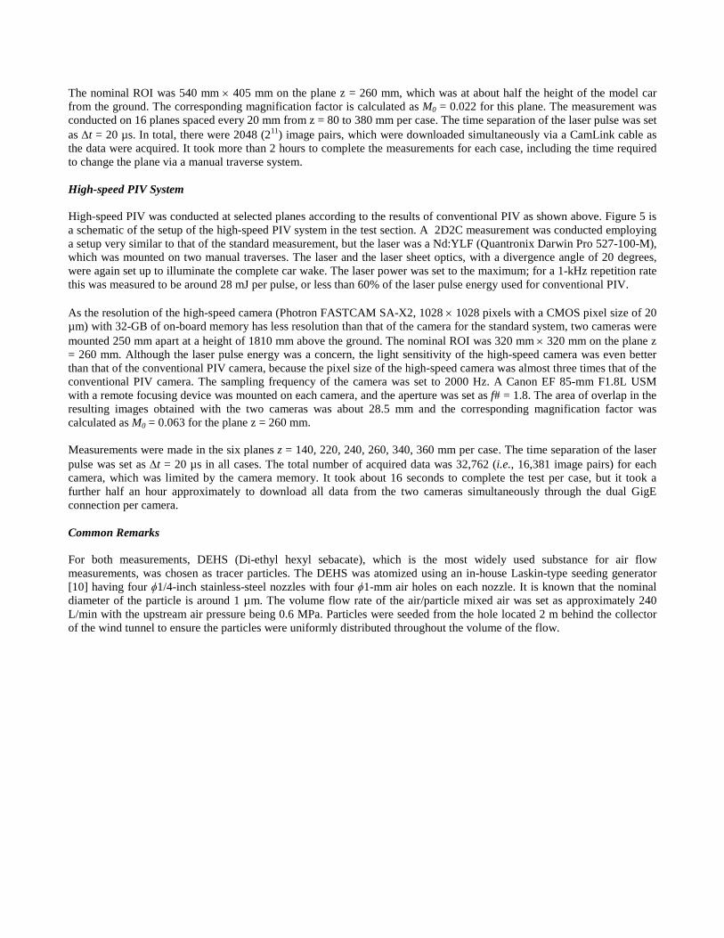
The nominal ROI was 540 mm × 405 mm on the plane z = 260 mm, which was at about half the height of the model car from the ground. The corresponding magnification factor is calculated as M0 = 0.022 for this plane. The measurement was conducted on 16 planes spaced every 20 mm from z = 80 to 380 mm per case. The time separation of the laser pulse was set as ∆t = 20 µs. In total, there were 2048 (211) image pairs, which were downloaded simultaneously via a CamLink cable as the data were acquired. It took more than 2 hours to complete the measurements for each case, including the time required to change the plane via a manual traverse system. High-speed PIV System High-speed PIV was conducted at selected planes according to the results of conventional PIV as shown above. Figure 5 is a schematic of the setup of the high-speed PIV system in the test section. A 2D2C measurement was conducted employing a setup very similar to that of the standard measurement, but the laser was a Nd:YLF (Quantronix Darwin Pro 527-100-M), which was mounted on two manual traverses. The laser and the laser sheet optics, with a divergence angle of 20 degrees, were again set up to illuminate the complete car wake. The laser power was set to the maximum; for a 1-kHz repetition rate this was measured to be around 28 mJ per pulse, or less than 60% of the laser pulse energy used for conventional PIV. As the resolution of the high-speed camera (Photron FASTCAM SA-X2, 1028 × 1028 pixels with a CMOS pixel size of 20 µm) with 32-GB of on-board memory has less resolution than that of the camera for the standard system, two cameras were mounted 250 mm apart at a height of 1810 mm above the ground. The nominal ROI was 320 mm × 320 mm on the plane z = 260 mm. Although the laser pulse energy was a concern, the light sensitivity of the high-speed camera was even better than that of the conventional PIV camera, because the pixel size of the high-speed camera was almost three times that of the conventional PIV camera. The sampling frequency of the camera was set to 2000 Hz. A Canon EF 85-mm F1.8L USM with a remote focusing device was mounted on each camera, and the aperture was set as f# = 1.8. The area of overlap in the resulting images obtained with the two cameras was about 28.5 mm and the corresponding magnification factor was calculated as M0 = 0.063 for the plane z = 260 mm. Measurements were made in the six planes z = 140, 220, 240, 260, 340, 360 mm per case. The time separation of the laser pulse was set as ∆t = 20 µs in all cases. The total number of acquired data was 32,762 (i.e., 16,381 image pairs) for each camera, which was limited by the camera memory. It took about 16 seconds to complete the test per case, but it took a further half an hour approximately to download all data from the two cameras simultaneously through the dual GigE connection per camera. Common Remarks For both measurements, DEHS (Di-ethyl hexyl sebacate), which is the most widely used substance for air flow measurements, was chosen as tracer particles. The DEHS was atomized using an in-house Laskin-type seeding generator [10] having four ϕ1/4-inch stainless-steel nozzles with four ϕ1-mm air holes on each nozzle. It is known that the nominal diameter of the particle is around 1 µm. The volume flow rate of the air/particle mixed air was set as approximately 240 L/min with the upstream air pressure being 0.6 MPa. Particles were seeded from the hole located 2 m behind the collector of the wind tunnel to ensure the particles were uniformly distributed throughout the volume of the flow.

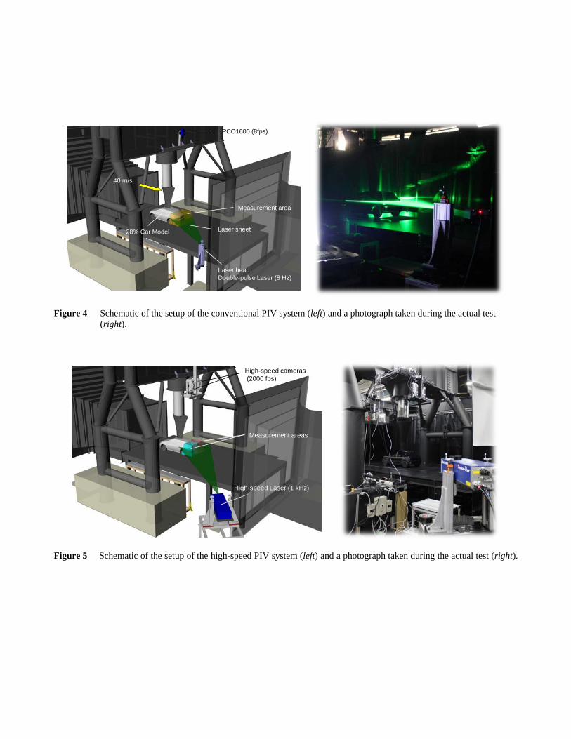
Figure 4 Schematic of the setup of the conventional PIV system (left) and a photograph taken during the actual test (right).

Figure 5 Schematic of the setup of the high-speed PIV system (left) and a photograph taken during the actual test (right).

PCO1600 (8fps)

28% Car Model Laser sheet

Laser head Double-pulse Laser (8 Hz)

Measurement area

40 m/s

Measurement areas

High-speed Laser (1 kHz)

High-speed cameras(2000 fps)

3. ANALYSIS 3.1. PIV Image Processing Conventional PIV The 2048 pairs of particle images collected in conventional PIV were post-processed. Although the maximum laser power with the optimum expansion of the laser sheet made it barely possible to capture entire flow fields; image preprocessing was still required to improve the quality of the resulting vector fields. First, image intensity normalization was applied to the raw particle images with a scale length of 5 pixels, and a sliding background filter with a length scale of 2 pixels was used to minimize the background intensity fluctuation due to laser reflections, which was useful for some planes. After applying the mask to the model shape for each plane, the pre-processed particle image pairs were processed to obtain vector fields. The interrogation algorithm is based on standard fast Fourier transform (FFT)-based cross-correlation with multi-pass window deformations and a decreasing window size. The initial interrogation window size was set to 32 × 32 pixels with a rectangular weight and 50% overlap, and the second and third passes were then made with a 16 × 16-pixel window with a circular weight and 50% overlap. Spurious vectors were replaced and interpolated back iteratively based on the root mean square (RMS) values of average displacement. The resulting spatial resolution was 2.7 mm at the representative plane z = 260 mm. High-speed PIV The 32,762 consecutive particle images collected in high-speed PIV were batch processed using PIVView2C Version 2.3, and an associated scheduler (ILA). As the particle images from high-speed PIV had relatively good quality, no preprocessing was necessary; only applied a mask to the model shape, where there were no particles. By making a pair from two consecutive camera frames, the raw images were post-processed with a standard FFT-based cross-correlation algorithm with uniform weighting. For interrogation, a multi-grid image deformation interrogation algorithm was chosen. The initial interrogation window size was set to 96 × 96 pixels and the window was iteratively reduced to 24 × 24 pixels with sixteen pixels (67%) of overlap, three iterations were conducted for the final resolution. Sub-pixel image shifting was achieved with third-order B-spline interpolation. For subpixel fitting, a 2D least-squares Gaussian fit with 3 × 3 neighboring points was used. Resulting pixel-based vector fields were post-processed with an outlier detection filter, by setting the maximum displacement difference of 4 pixels and the normalized median threshold of 3.5. The use of second order correlation peaks was enabled. Outliers were then replaced and interpolated, by re-evaluating with a larger interrogation window. The number of validation passes was set to five. The resulting spatial resolution was 2.62 mm at the representative plane z = 260 mm.

3.2. Spectral Analysis Aerodynamic Loads Aerodynamic loads 𝐹𝐹𝑖𝑖(𝑡𝑡) or 𝑀𝑀𝑖𝑖(𝑡𝑡) measured by the six-component load cell were processed to calculate the average 𝐹𝐹𝑖𝑖 or 𝑀𝑀𝑖𝑖 , and the RMS of the fluctuation (𝐹𝐹𝑖𝑖′)𝑟𝑟𝑟𝑟𝑟𝑟 or (𝑀𝑀𝑖𝑖

′)𝑟𝑟𝑟𝑟𝑟𝑟 of each load was computed. Additionally, this zero-mean fluctuation of each component was used to conduct spectral analysis. The periodogram was calculated from 32,768 time records, with 50% overlap of Hamming window, using Welch method. Using a 2048-point periodogram, the corresponding frequency resolution was 0.488 Hz. Thirty data segments were averaged in the resulting periodogram. Prior to computing the fluctuations, aerodynamic load data were low-pass filtered to avoid potentially erroneous results above 8 Hz due to noise from resonance of the mechanical system as shown in §2.2. The low-pass filter was designed using a tenth-order Butterworth digital IIR filter with the pole-zero placement method. The first 300 data points were removed to avoid initial oscillations which are attributed to the initial rise time of the filter. PIV data The average of the velocity field 𝑢𝑢𝑖𝑖(𝑥𝑥, 𝑦𝑦) was computed from the post-processed velocity time records 𝑢𝑢𝑖𝑖(𝑥𝑥, 𝑦𝑦, 𝑡𝑡) at each grid point (𝑥𝑥,𝑦𝑦) , and 𝑢𝑢𝑖𝑖(𝑥𝑥, 𝑦𝑦) was then subtracted from 𝑢𝑢𝑖𝑖(𝑥𝑥, 𝑦𝑦, 𝑡𝑡) to obtain the zero-mean fluctuation component 𝑢𝑢𝑖𝑖′(𝑥𝑥, 𝑦𝑦, 𝑡𝑡) in the time records. The RMS of the fluctuation of each component velocity (𝑢𝑢𝑖𝑖′)𝑟𝑟𝑟𝑟𝑟𝑟 was then computed to give the turbulence intensity. The periodograms were then calculated from 16,381 time records, using 50% overlap of the Hamming window, using Welch method. Similar to the above processing of the aerodynamic load data, 2048-point periodograms were used to extract the low-frequency data, giving a frequency resolution of 0.488 Hz. The total number of segments used in averaging was reduced to 14, which is still a reasonable number with which to observe a relative change in the power density spectrum (PSD) and thus determine the effects of aerodynamic devices. For the following discussions, most of the obtained data were spectrally filtered to extract the large-scale motion of the flow, which presumably affects the drivability of the car. First, the zero-mean fluctuation component of the post-processed velocity components was low-pass filtered digitally with a tenth-order Butterworth filter having a cut-off frequency of 2 Hz as was used for aerodynamic loads. These filtered data were then added back to the mean values to reconstruct filtered velocity fields and create the animation. Note that the first 300 points of resulting data were removed to avoid oscillation as mentioned above. 3.3. Spatial Correlations for the Flow Field As the current study focuses on the large-scale lateral motion of the wake that takes place alternately left and right, the low-pass filtered velocity data in time records were analyzed to investigate the coherence of the flow between the two sides of the car model. To this end, cross-correlation coefficients 𝑅𝑅𝑢𝑢𝑖𝑖𝑢𝑢𝑖𝑖(𝑥𝑥, 𝑦𝑦, 𝜏𝜏) of each component of velocity fluctuation 𝑢𝑢𝑖𝑖′(𝑥𝑥, 𝑦𝑦, 𝑡𝑡) at each grid point (𝑥𝑥, 𝑦𝑦) were calculated with respect to each component of the velocity fluctuation 𝑢𝑢𝑖𝑖′(𝑥𝑥𝑟𝑟𝑟𝑟𝑟𝑟 ,𝑦𝑦𝑟𝑟𝑟𝑟𝑟𝑟 , 𝑡𝑡) at the reference point (𝑥𝑥𝑟𝑟𝑟𝑟𝑟𝑟 ,𝑦𝑦𝑟𝑟𝑟𝑟𝑟𝑟), using the following equations. The details of the reference points are given in later sections. The current analysis was only conducted by considering the lag time τ = 0 for simplicity; i.e., only considering correlations that occur simultaneously in the field. These correlation coefficients can be plotted as a coefficient map, the distribution of which gives an overview of the unsteadiness of the wake.

𝑅𝑅𝑢𝑢𝑖𝑖𝑢𝑢𝑖𝑖(𝑥𝑥, 𝑦𝑦, 𝜏𝜏) =𝑢𝑢𝑖𝑖′(𝑥𝑥𝑟𝑟𝑟𝑟𝑟𝑟 , 𝑦𝑦𝑟𝑟𝑟𝑟𝑟𝑟 , 𝑡𝑡)𝑢𝑢𝑖𝑖′(𝑥𝑥, 𝑦𝑦, 𝑡𝑡 + 𝜏𝜏)

�𝑢𝑢𝑖𝑖′(𝑥𝑥𝑟𝑟𝑟𝑟𝑟𝑟 , 𝑦𝑦𝑟𝑟𝑟𝑟𝑟𝑟 , 𝑡𝑡)2�𝑢𝑢𝑖𝑖′(𝑥𝑥, 𝑦𝑦, 𝑡𝑡)2 (1)

4. RESULTS AND DISCUSSION, PART 1: Comparisons between Conventional and High-Speed PIVs for the Baseline Case

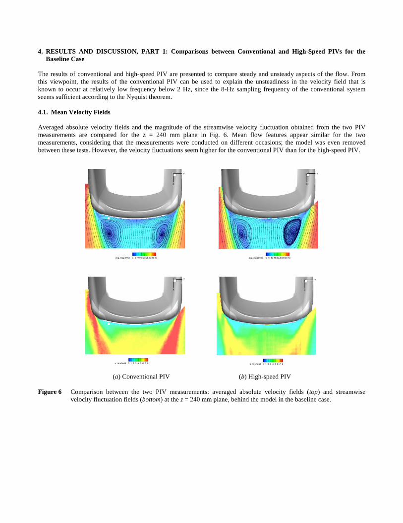
The results of conventional and high-speed PIV are presented to compare steady and unsteady aspects of the flow. From this viewpoint, the results of the conventional PIV can be used to explain the unsteadiness in the velocity field that is known to occur at relatively low frequency below 2 Hz, since the 8-Hz sampling frequency of the conventional system seems sufficient according to the Nyquist theorem. 4.1. Mean Velocity Fields Averaged absolute velocity fields and the magnitude of the streamwise velocity fluctuation obtained from the two PIV measurements are compared for the z = 240 mm plane in Fig. 6. Mean flow features appear similar for the two measurements, considering that the measurements were conducted on different occasions; the model was even removed between these tests. However, the velocity fluctuations seem higher for the conventional PIV than for the high-speed PIV.

(a) Conventional PIV (b) High-speed PIV Figure 6 Comparison between the two PIV measurements: averaged absolute velocity fields (top) and streamwise

velocity fluctuation fields (bottom) at the z = 240 mm plane, behind the model in the baseline case.

4.2. Unsteady Aerodynamic Characteristics of the Wake Obtained from Filtered Instantaneous Flow Fields To better understand the unsteady flow characteristics, spectral analysis was first conducted for the data of high-speed PIV. Time records of streamwise velocity data u(t) were chosen at the point (x,y) = (1200,220) inside the shear layer, and the PSD was calculated. Results are summarized in Fig. 7. It is seen that the dominant fluctuation occurred at frequencies lower than 2 Hz (i.e., St < 0.02), which is consistent with the hotwire measurement in the previous study [2]. To clearly extract low-frequency flow characteristics, a low-pass filter with a cut-off frequency of 2 Hz was applied to each component of the resulting velocity fluctuation 𝑢𝑢𝑖𝑖′(𝑥𝑥, 𝑦𝑦, 𝑡𝑡) at each grid point as mentioned in detail in §3.2 for both measurement cases, and time-series velocity fields were reconstructed finally. Figure 8 shows a resulting snapshot of the instantaneous filtered velocity field for each measurement. The velocity field of the conventional PIV appears like a typical snapshot of the pre-filtered flow field, whereas the flow field of the high-speed PIV resembles that of the mean flow field. Figure 9 shows a series of frames of low-pass filtered instantaneous flow fields obtained from high-speed PIV at four different instances. It is seen that the wake flow indeed sways left and right behind the model and the sweep takes approximately 1 s, which corresponds to the peak in the PSD in Fig. 7.

Figure 7 PSD distribution of the streamwise velocity u at the selected point (x,y) = (1200, 220) in the shear layer on the z = 240 mm plane for the baseline case.

(a) Conventional PIV (b) High-speed PIV Figure 8 Instantaneous filtered flow fields for the baseline case obtained using the (a) conventional and (b) high-speed

system. Note that the cut-off frequency was set at 2 Hz to remove higher components of the velocity as seen in Fig. 7.

Cut-off frequency 100Hz

Cut-off frequency 2Hz

(1200,220)

(c) t = 10.14 s (d) t = 10.50 s Figure 9 Timeline snapshots of the low-pass filtered instantaneous flow fields with streamlines for the baseline case

obtained from the high-speed PIV. The contour plots indicate the magnitude of the average velocity, showing a clear swaying motion of the wake. These results underline the advantage of high-speed PIV over conventional PIV with low sampling frequency, and the single-point hotwire measurement.

4.3. Assessment of the Sampling Frequency and Aliasing Effect in Spatial Correlations Using the reconstructed velocity fields after rejecting higher-frequency velocity fluctuations for both measurement cases, two-point spatial cross-correlations 𝑅𝑅𝑢𝑢𝑢𝑢(𝑥𝑥, 𝑦𝑦, 0) of the streamwise velocity fluctuation were calculated using eq. (1) as shown in §3.3 for the entire measurement field. The correlation coefficients are based on the reference point shown in Fig. 7. Results are summarized in Fig. 10. In the baseline configuration, the resulting coefficient maps for high-speed PIV showed opposite signs either side of the wake, as expected. In contrast, for conventional PIV, only weak correlation is found. To understand these results more in detail, similar maps were created by reducing number of samples at each grid point of the vector fields, to regenerate the data with lower sampling frequency, as shown in Fig. 11. The coefficients gradually decreased as the sampling frequency decreased, approaching those for the conventional PIV as shown in Fig. 10a. The above result indicates that the 8-Hz sampling frequency of the conventional system is insufficient owing to aliasing effects of flow fluctuations that occur at frequencies of 4 Hz or above. Judging from the color distribution of the contour map in Fig. 11, the sampling frequency must therefore be somewhere between 250 and 500 Hz, even if low-frequency phenomena around 1 Hz are of interest. This explains why the fluctuation level for conventional PIV was higher than that for the high-speed PIV.

(a) t = 9.09 s (b) t = 9.54 s

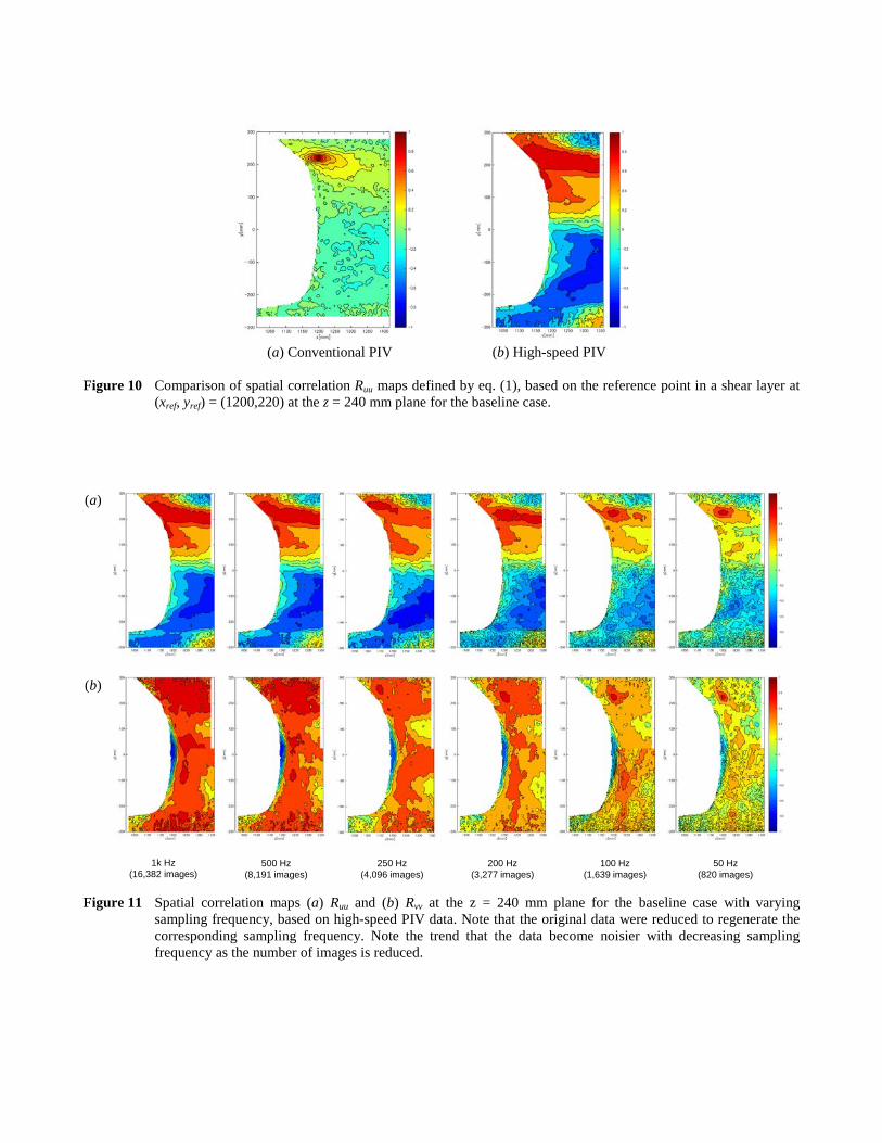
(a) Conventional PIV (b) High-speed PIV Figure 10 Comparison of spatial correlation Ruu maps defined by eq. (1), based on the reference point in a shear layer at

(xref, yref) = (1200,220) at the z = 240 mm plane for the baseline case.

Figure 11 Spatial correlation maps (a) Ruu and (b) Rvv at the z = 240 mm plane for the baseline case with varying sampling frequency, based on high-speed PIV data. Note that the original data were reduced to regenerate the corresponding sampling frequency. Note the trend that the data become noisier with decreasing sampling frequency as the number of images is reduced.

1k Hz(16,382 images)

500 Hz(8,191 images)



50 Hz(820 images)


(a)

(b)

5. RESULTS AND DISCUSSION, PART 2: Effects of Aerodynamic Devices on Unsteadiness of the Wake This chapter focuses on the effects of aerodynamic devices, as shown in §2.3, on unsteady features of the aerodynamic loads and velocity fields by comparing with results for the baseline case. 5.1. Aerodynamic Loads Results of the aerodynamic load measurements, which were made four times simultaneously with PIV measurements, are shown in Fig. 12. Figure 12a shows the difference in mean aerodynamic coefficients for each aerodynamic device relative to the baseline case. It is seen that each aerodynamic device is surprisingly insensitive to the lateral direction of the load; see, for example, Cy and CMz. It is interesting to note that the combi-VG even has a neutral effect on the drag coefficient Cx. Figure 14b shows the percentage change in aerodynamic-load fluctuations. The aerodynamic devices reduce of the fluctuations on the baseline by approximately 30%. The combi-spoiler reduces the fluctuations more than the combi-VG in the lateral directions (see results for the side force Fy, the roll moment Mx, and the yaw moment Mz) whereas the combi-VG reduces fluctuations even in the vertical direction (see results for the vertical force Fz and the pitch moment My) in addition to the lateral forces and moments. To clarify the frequency information of these effects, the PSD was calculated for each component of the aerodynamic loads. Results are shown in Fig. 13. The reduction in the fluctuation as seen in Fig. 12b occurs below a frequency of 2 Hz, which corresponds to the Strouhal number 𝑆𝑆𝑡𝑡< 0.02.

Figure 12 Influence of aerodynamic devices (a) on each aerodynamic coefficient and (b) on the fluctuation levels of each aerodynamic load after applying an 8-Hz low-pass filter to avoid mechanical resonance of the system. Note that error bars are based on results for four instances.

(a) (b)

Figure 13 Effects of the aerodynamic devices on the PSD distribution of each aerodynamic load.

(a)

(b)

(c)

(d)

(e)

(f)

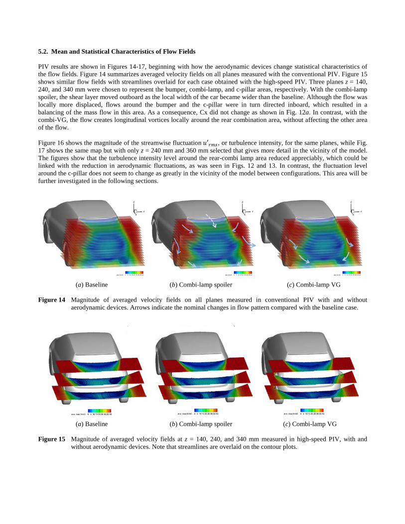
5.2. Mean and Statistical Characteristics of Flow Fields PIV results are shown in Figures 14-17, beginning with how the aerodynamic devices change statistical characteristics of the flow fields. Figure 14 summarizes averaged velocity fields on all planes measured with the conventional PIV. Figure 15 shows similar flow fields with streamlines overlaid for each case obtained with the high-speed PIV. Three planes z = 140, 240, and 340 mm were chosen to represent the bumper, combi-lamp, and c-pillar areas, respectively. With the combi-lamp spoiler, the shear layer moved outboard as the local width of the car became wider than the baseline. Although the flow was locally more displaced, flows around the bumper and the c-pillar were in turn directed inboard, which resulted in a balancing of the mass flow in this area. As a consequence, Cx did not change as shown in Fig. 12a. In contrast, with the combi-VG, the flow creates longitudinal vortices locally around the rear combination area, without affecting the other area of the flow. Figure 16 shows the magnitude of the streamwise fluctuation 𝑢𝑢′𝑟𝑟𝑟𝑟𝑟𝑟, or turbulence intensity, for the same planes, while Fig. 17 shows the same map but with only z = 240 mm and 360 mm selected that gives more detail in the vicinity of the model. The figures show that the turbulence intensity level around the rear-combi lamp area reduced appreciably, which could be linked with the reduction in aerodynamic fluctuations, as was seen in Figs. 12 and 13. In contrast, the fluctuation level around the c-pillar does not seem to change as greatly in the vicinity of the model between configurations. This area will be further investigated in the following sections.


Figure 14 Magnitude of averaged velocity fields on all planes measured in conventional PIV with and without

aerodynamic devices. Arrows indicate the nominal changes in flow pattern compared with the baseline case.


Figure 15 Magnitude of averaged velocity fields at z = 140, 240, and 340 mm measured in high-speed PIV, with and

without aerodynamic devices. Note that streamlines are overlaid on the contour plots.


Figure 16 Streamwise fluctuation 𝑢𝑢′𝑟𝑟𝑟𝑟𝑟𝑟 at z = 140, 240, and 340 mm, with different aerodynamic devices after a low-

pass filter was applied with a cut-off frequency of 2 Hz to capture low-frequency fluctuations.

at z = 240 mm

at z = 340 mm

(a) Baseline (b) Combi-lamp spoiler (c) Combi-lamp VG Figure 17 Two-dimensional contour plot of streamwise fluctuation 𝑢𝑢′𝑟𝑟𝑟𝑟𝑟𝑟 at z = 240 mm (top) and 340 mm (bottom)

obtained from the results in Fig. 16.

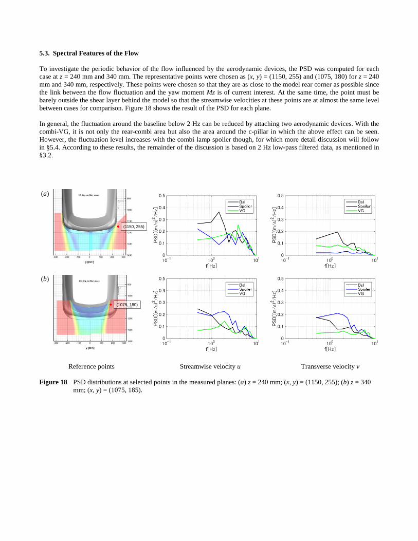
5.3. Spectral Features of the Flow To investigate the periodic behavior of the flow influenced by the aerodynamic devices, the PSD was computed for each case at z = 240 mm and 340 mm. The representative points were chosen as (x, y) = (1150, 255) and (1075, 180) for z = 240 mm and 340 mm, respectively. These points were chosen so that they are as close to the model rear corner as possible since the link between the flow fluctuation and the yaw moment Mz is of current interest. At the same time, the point must be barely outside the shear layer behind the model so that the streamwise velocities at these points are at almost the same level between cases for comparison. Figure 18 shows the result of the PSD for each plane. In general, the fluctuation around the baseline below 2 Hz can be reduced by attaching two aerodynamic devices. With the combi-VG, it is not only the rear-combi area but also the area around the c-pillar in which the above effect can be seen. However, the fluctuation level increases with the combi-lamp spoiler though, for which more detail discussion will follow in §5.4. According to these results, the remainder of the discussion is based on 2 Hz low-pass filtered data, as mentioned in §3.2.

Reference points Streamwise velocity u Transverse velocity v

Figure 18 PSD distributions at selected points in the measured planes: (a) z = 240 mm; (x, y) = (1150, 255); (b) z = 340

mm; (x, y) = (1075, 185).

(1150, 255)

(1075, 180)

(a)

(b)

5.4. Correlations of Velocity Fields After applying the low-pass filter with a cut-off frequency of 2 Hz to the vector fields of high-speed PIV, two-point correlation coefficients of each component of the velocity fluctuation Ruu and Rvv were calculated using eq. (1), as described in §3.3, with respect to the reference point, as summarized in Table 3. To find a reference point on each plane, points at different transversal positions were investigated. It was found that the basic relations between cases with and without aerodynamic devices did not change even though the location changed as long as the point remained on the freestream side of the shear layer. Reference points on each plane are thus defined as summarized in Table 3. The resulting contour maps are presented in Fig. 19 and Fig. 20 for z = 240 mm and 340 mm planes, respectively, while Fig. 21 presents coefficient contour maps for all planes in three dimensions, but displaying the results where the coefficient coefficients are above 0.4 for Ruu and 0.6 for Rvv. The following observations can be made from these results: There is no clear trend of change around the bumper area; i.e., z = 140 mm. The flows in this area are already so

disturbed by the highly turbulent flow from the wheel well that this effect dominates any effect of the aerodynamic device.

For the baseline case, a broad area of negative correlation coefficients in Ruu can be seen in the combi-lamp area on the left; i.e., z = 240 mm plane. Additionally, the Rvv distribution has a completely positive region in the wake (see Figs. 19 and 21). These results indicate that the swaying motion of the flow as shown in Fig. 11 exists in this area. In contrast, a narrow band of uncorrelated area can be seen just outside the shear layer area around the c-pillar (i.e., z = 340 mm plane), and Rvv has clearly opposite signs on the left and right (see Fig. 20). This indicates that the fluctuation of the flow is symmetrical behind the car model.

In general, the two aerodynamic devices tend to weaken the correlations of Ruu and Rvv in the vicinity of the rear combi-lamp area on the rear left. The combi-VG seems to be more influential than the combi-spoiler in the vicinity of the model (see Figs. 19 and 21). However, when it comes to the c-pillar area, the two devices produce opposite trends, described as follows.

The combi-spoiler has positive Ruu on the left corner around the c-pillar, whereas slightly more negative values of Rvv are seen (see Figs. 20 and 21). These trends indicate that flow fluctuation is more symmetrical on the left and right sides of the car model. It is interesting that the fluctuation level of the flow is as high as seen in Fig. 18; however, as the fluctuation occurs in a symmetric manner, it is cancelling the yaw moment (Mz) fluctuations.

The combi-VG produces slightly more negative correlation in the Ruu map and less negative correlation in the Rvv map on the left corner around the c-pillar (see Fig. 20), indicating a possible effect on the fluctuation of Mz. However, as the fluctuation level of the flow with the combi-VG is so low, as shown in Fig. 18, the changes in correlation coefficient do not affect the flow enough to influence the fluctuation of Mz as a result.

Table 3 Reference points on each measurement plane

z [mm] Coordinate (xref, yref) [mm] 140，220, 240, 260 (1150, 255)

340, 360 (1075, 180)

𝑅𝑅𝑢𝑢𝑢𝑢

𝑅𝑅𝑣𝑣𝑣𝑣


Figure 19 Correlation map of velocity fluctuations at z = 240 mm.

𝑅𝑅𝑢𝑢𝑢𝑢

𝑅𝑅𝑣𝑣𝑣𝑣


Figure 20 Correlation map of velocity fluctuations at z = 340 mm.

Ruu Ruu Ruu-1 0 1 -1 0 1 -1 0 1

(xref, yref)

-1 0 1 -1 0 1 -1 0 1Ruu Ruu Ruu

(xref, yref)

𝑅𝑅𝑢𝑢𝑢𝑢 above 0.4

𝑅𝑅𝑣𝑣𝑣𝑣 above 0.6

(a) Baseline (b) Combi-lamp spoiler (c) Combi-lamp VG Figure 21 Correlation map for all planes. Note that the contour plots are only shown if the magnitude of the correlation

coefficients is higher than the indicated threshold values.

-1 0 1 -1 0 1 -1 0 1Ruu Ruu Ruu

-1 0 1 -1 0 1 -1 0 1Ruu Ruu Ruu

6. SUMMARY A 28%-scale wind tunnel car model based on a hatchback passenger car was investigated to clarify unsteady flow phenomena using conventional and high-speed PIV. The effects of two different aerodynamic devices were examined: a combi-lamp spoiler and a combi-lamp VG. These devices suppress relatively high aerodynamic load fluctuations compared with the baseline case. From the results of the current investigation, the following conclusions can be drawn: 1. By conducting high-speed PIV with a sampling frequency of 1 kHz, it was possible to capture a typical unsteady flow

phenomenon; i.e., a lateral swaying motion behind the car model having nominal frequency less than 2 Hz, or St < 0.02. These fluctuations can be detected by opposite signs in a spatial correlation map for the two sides of the car.

2. The unsteady effects cannot be captured using a conventional PIV system owing to the aliasing effect. By reducing the sampling rate of the original data and comparing the frequency contents, it was shown that a minimum sampling rate of 250 Hz is necessary to capture these phenomena.

3. The aerodynamic devices suppress the fluctuation of the flow around the rear combi-lamp area, which occurs at a frequency of less than 2 Hz, and the spatial correlations between the two sides of the model are weakened in this area as well.

4. The effects of these devices are different for the area around the c-pillar, as follows: (i) The combi-lamp spoiler results in slightly more fluctuations in this area, but the correlation coefficient has the

same sign, which cancels the effect on the yaw moment. (ii) The combi-VG makes the correlation slightly negative, but the fluctuation is suppressed so much that the

fluctuation of the yaw moment may be unaffected. The fluctuations are presumably due to the unsteady behavior of the flow around the rear combi-lamp; however, the cause of negative correlations between the two sides of the car is still unknown and requires further investigation. Furthermore, the reason why the Strouhal number at which the swaying motion occurs behind the model is so low compared with values in other studies, typically around St = 0.1, needs to be investigated. REFERENCES [1] Simis-Williams D, Dominy R, and Howell J “An Investigation into Large Scale Unsteady Structures in the Wake of Real and Idealized

Hatchback Car Models” SAE Technical Paper 2001-01-1041 (2001) [2] Kawakami M et al “Improvement in vehicle motion performance by suppression of aerodynamic load fluctuations” SAE Int J Passeng Cars

– Mech. Syst. 8(1) (2015) pp.205-216 [3] Ishima T, Takahashi Y, Okado H, Baba Y, and Obokata T “3D-PIV Measurement and Visualization of Streamlines Around a Standard SAE

Vehicle Model” SAE Technical Paper 2011-01-0161 (2011)

[4] Strangfeld C, Wieser D, Schmidt H-J, Woszidlo R, Nayeri C, and Paschereit C “Experimental Study of Baseline Flow Characteristics for the Realistic Car Model DrivAer” SAE Technical Paper 2013-01-1251 (2013)

[5] Cardano D, Carlino G, and Cogotti “PIV in the car industry: state-of-the-art and future perspectives” Particle Image Velocimetry, Topic Appl Physics 112 (2008) pp.363-376

[6] Volpe R, Dvinant P, and Kourta A “Experimental characterization of the unsteady natural wake of the full‑scale square back Ahmed body:

flow bi‑stability and spectral analysis” Exp in Fluids (2015) pp.56-99. [7] Kohri I, Yamanashi T, Nasu T, Hashizume Y, et al "Study on the transient behaviour of the vortex structure behind Ahmed body" SAE Int J

Passeng Cars – Mech. Syst. 7(2) (2014) pp.586-602 [8] Wernet MP “Temporally resolved PIV for space-time correlations in both cold and hot jet flows” Meas Sci Technol 18 (2007) pp.1387-1403 [9] Kuroyanagi H, Murata O, Kawakami M, Nakagawa M, Kato Y, and Yoshida K “25% Scale Automotive Wind Tunnel with a 6-DOF High

Response Model Shaker” Proc JSAE Annu Congr 107-12, Paper No. 20125785 (2012) (in Japanese) [10] Kaehler CJ, Sammler B, and Kompenhans J “Generation and control of tracer particles for optical flow investigations in air” Exp in Fluids

33 (2002) pp.736-742

unsteady flow measurements in the wake behind a wind...

Documents