unraveling urban traffic flows
TRANSCRIPT

UnravellingUrbanTrafficFlows
From new insights to advanced solutions… a work in progress Prof. dr. Serge Hoogendoorn
1

AMSTERDAM INSTITUTE FOR
ADVANCED METROPOLITAN SOLUTIONS
TU DELFT, WAGENINGEN UR, MIT
ACCENTURE, ALLIANDER, AMSTERDAM
SMART CITY, CISCO, CITY OF BOSTON,
ESA, IBM, KPN, SHELL, TNO, WAAG SOCIETY,
WATERNET
CITY METABOLISM: URBAN FLOWS WATER-ENERGY-WASTE-FOOD-DATA-PEOPLE
2
CIRCULAR CITY
VITAL CITY
CONNECTED CITY
Circular economyWater, energy, food, waste
Smart infrastructures
Urban big dataInternet of Everything
Digital fabricationSmart mobility
Resilient, clean and healthy urban environmentBlue-green infrastructuresSocial & responsible design
Proposition: using the city as a living lab to explore impact and find possibilities of these (and other) trends on mobility and other sectors…

3
AMSTERDAM INSTITUTE FOR
ADVANCED METROPOLITAN SOLUTIONS
TU DELFT, WAGENINGEN UR, MIT
ACCENTURE, ALLIANDER, AMSTERDAM
SMART CITY, CISCO, CITY OF BOSTON,
ESA, IBM, KPN, SHELL, TNO, WAAG SOCIETY,
WATERNET
AMBITIONS
An internationally renowned, public-private institution in the area of metropolitan solutions that in 2022 has …
… 200-250 talented students participating in a new MSc …
… 100-150 researchers working on discovering, developing and implementing metropolitan solutions …
… EUR 25-35 million annual budget for research and valorization …
… 30-50 public and private partners participating ...
… 500-1,000 publications, 10-15 spin-outs and 30-70 start-ups generated between 2013 and 2022 …
… an excellent position for continued value creation in the next 20 years.

Enteringtheurbanage
• Urbanisation is a global trend: more people live in cities than ever!
• City regions become focal points of the world economy in terms of output, productivity, decision making power, innovation power
• Requirement for success: internal connectivity (within city or city region) and external connectivity (airport, ports): importance of accessibility
4

Challenges…
• Accessibilityisamajorissueinmanycities(Amsterdam,Melbourne)
• Mostdelaysareexperiencedincities(notonfreeways!),yetfreewayshavereceivedmuchattentioninthepast…
• Atthesametime,(re-)urbanisationopensupmanynewalleywaysforsustainablemobility(activemodes,seamlessmulti-modaltransport,sharedmobility,autonomousdriving)
• Sowhatdoweseeaskeythemes?
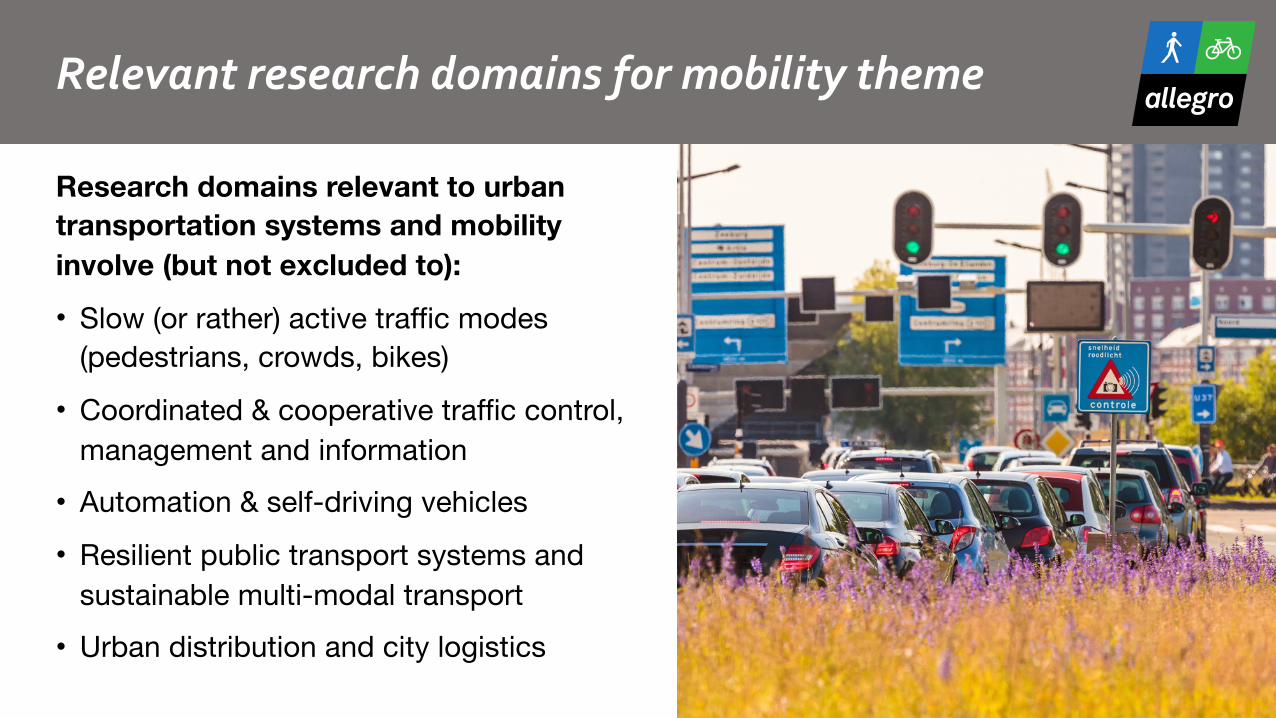
Relevantresearchdomainsformobilitytheme
Research domains relevant to urban transportation systems and mobility involve (but not excluded to): • Slow (or rather) active traffic modes
(pedestrians, crowds, bikes)
• Coordinated & cooperative traffic control, management and information
• Automation & self-driving vehicles
• Resilient public transport systems and sustainable multi-modal transport
• Urban distribution and city logistics7
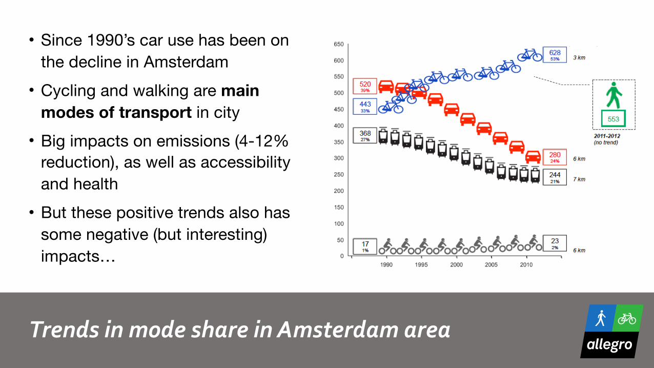
TrendsinmodeshareinAmsterdamarea
• Since 1990’s car use has been on the decline in Amsterdam
• Cycling and walking are main modes of transport in city
• Big impacts on emissions (4-12% reduction), as well as accessibility and health
• But these positive trends also has some negative (but interesting) impacts…
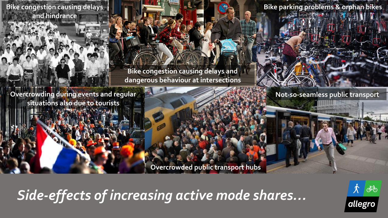
Side-effectsofincreasingactivemodeshares…
Bikecongestioncausingdelaysandhindrance
Overcrowdingduringeventsandregularsituationsalsoduetotourists
Overcrowdedpublictransporthubs
Not-so-seamlesspublictransport
Bikeparkingproblems&orphanbikes
Bikecongestioncausingdelaysanddangerousbehaviouratintersections
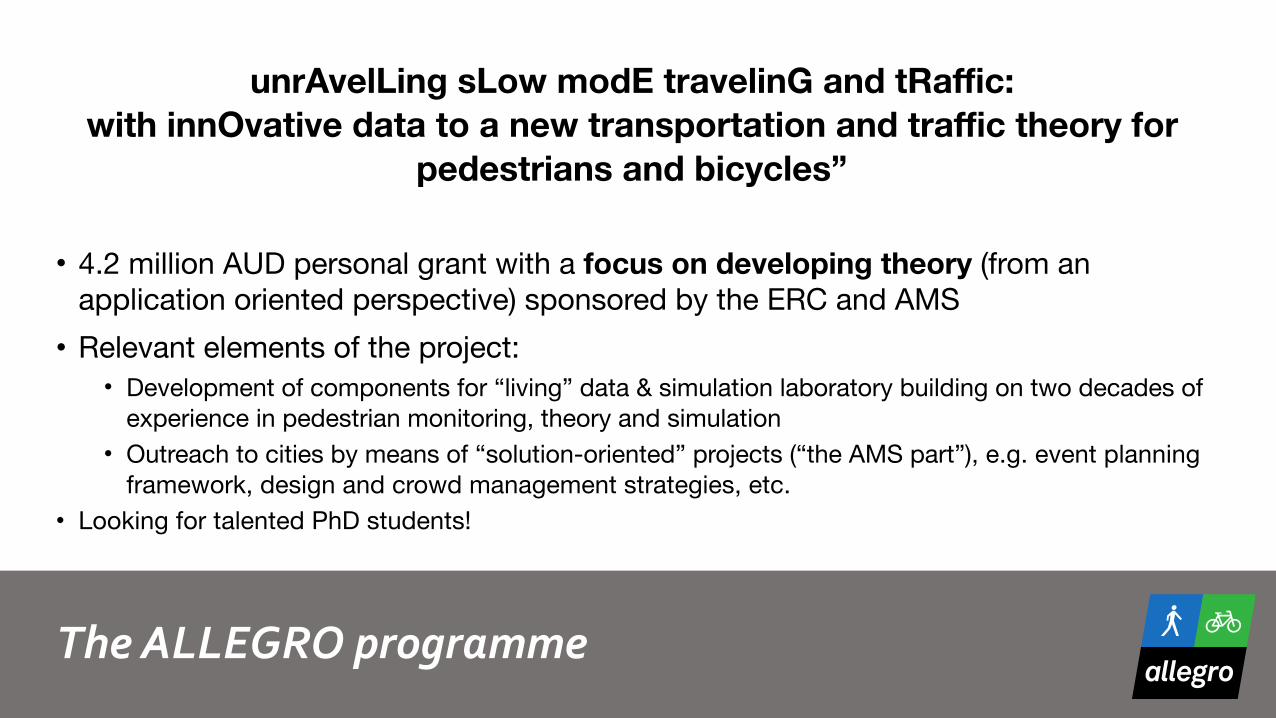
TheALLEGROprogramme
unrAvelLing sLow modE travelinG and tRaffic: with innOvative data to a new transportation and traffic theory for
pedestrians and bicycles”
• 4.2 million AUD personal grant with a focus on developing theory (from an application oriented perspective) sponsored by the ERC and AMS
• Relevant elements of the project: • Development of components for “living” data & simulation laboratory building on two decades of
experience in pedestrian monitoring, theory and simulation• Outreach to cities by means of “solution-oriented” projects (“the AMS part”), e.g. event planning
framework, design and crowd management strategies, etc.• Looking for talented PhD students!
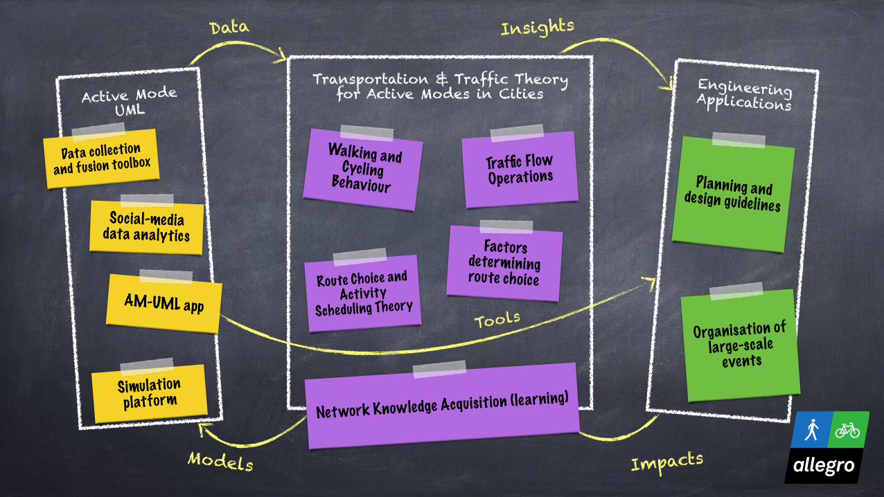
Active Mode UML
Engineering Applications
Transportation & Traffic Theory for Active Modes in Cities
Data collection and fusion toolbox
Social-media data analytics
AM-UML app
Simulation platform
Walking and Cycling BehaviourTraffic Flow Operations
Route Choice and Activity
Scheduling Theory
Planning and design guidelines
Organisation of large-scale
events
Data Insights
Tools
Models Impacts
Network Knowledge Acquisition (learning)
Factors determining route choice

12Engineering the future city.
Today’stalk
• Focusonactivemodesinparticularonpedestrianandcrowds
• UseSAILeventasthedrivingexampletoillustratevariousconceptsinmonitoringandmanagement
• SAILprojectentaileddevelopmentofacrowdmanagementdecisionsupportsystem
13
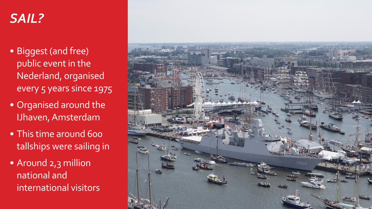
SAIL?
• Biggest(andfree)publiceventintheNederland,organisedevery5yearssince1975
• OrganisedaroundtheIJhaven,Amsterdam
• Thistimearound600tallshipsweresailingin
• Around2,3millionnationalandinternationalvisitors

14
Engineeringchallenges foreventsorregularsituations…• Canweforacertaineventpredictifasafetyorthroughputissuewilloccur?
• Canwedevelopmethodstosupportorganisation,planninganddesign?
• Canwedevelopapproachestoreal-timemanagelargepedestrianflowssafelyandefficiently?
• Canweensurethatallofthesearerobustagainsunforeseencircumstances?
Deepknowledgeofcrowddynamicsisessentialtoanswerthesequestions!

Pedestrianflowoperations…
Simple case example: how long does it take to evacuatie a room? • Consider a room of N people• Suppose that the (only) exit has capacity of C Peds/hour• Use a simple queuing model to compute duration T• How long does the evacuation take?
• Capacity of the door is very important• Which factors determine capacity?
15
T =N
C
Npeopleinarea
Doorcapacity:C
N
C
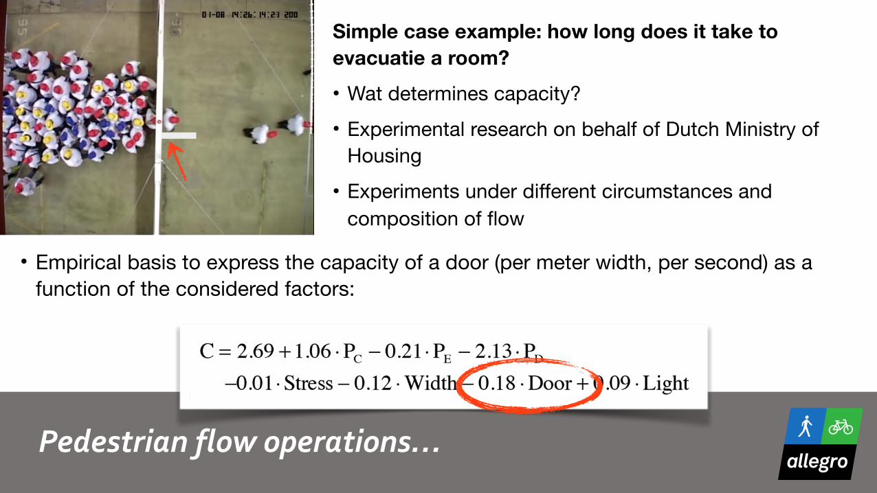
Pedestrianflowoperations…
Simple case example: how long does it take to evacuatie a room? • Wat determines capacity?• Experimental research on behalf of Dutch Ministry of
Housing• Experiments under different circumstances and
composition of flow
• Empirical basis to express the capacity of a door (per meter width, per second) as a function of the considered factors:
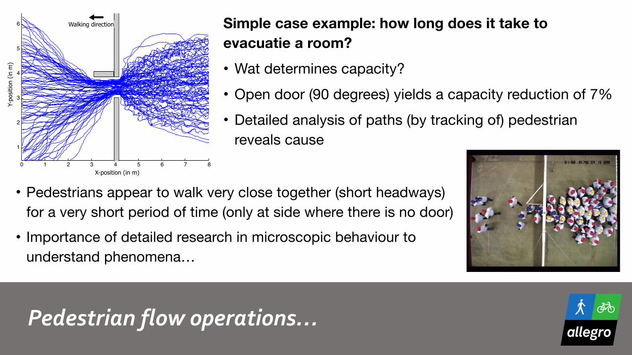
Pedestrianflowoperations…
Simple case example: how long does it take to evacuatie a room? • Wat determines capacity?• Open door (90 degrees) yields a capacity reduction of 7%• Detailed analysis of paths (by tracking of) pedestrian
reveals cause0 1 2 3 4 5 6 7 8
1
2
3
4
5
6 Looprichting
X-positie (in m)
Y-positie (in m) Walking direction
X-position (in m)
Y-po
sitio
n (in
m)
• Pedestrians appear to walk very close together (short headways) for a very short period of time (only at side where there is no door)
• Importance of detailed research in microscopic behaviour to understand phenomena…
18
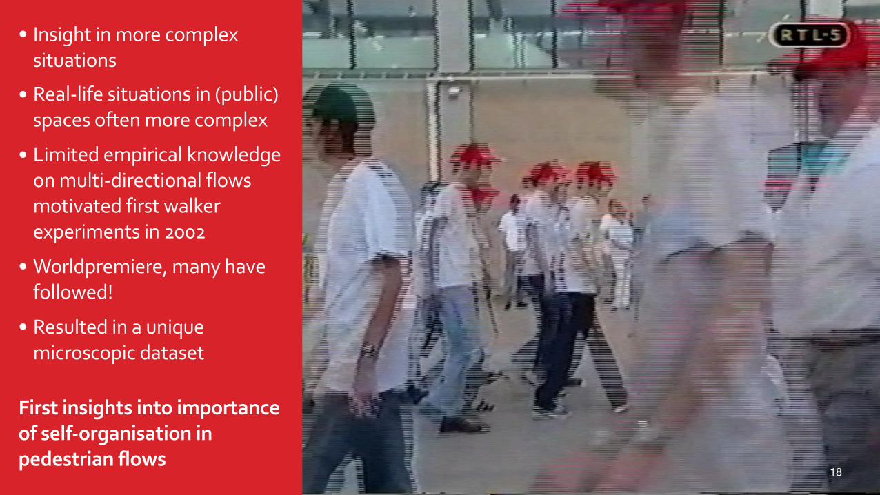
• Insightinmorecomplexsituations
• Real-lifesituationsin(public)spacesoftenmorecomplex
• Limitedempiricalknowledgeonmulti-directionalflowsmotivatedfirstwalkerexperimentsin2002
• Worldpremiere,manyhavefollowed!
• Resultedinauniquemicroscopicdataset
Firstinsightsintoimportanceofself-organisationinpedestrianflows

Fascinatingself-organisation
• Example efficient self-organisation dynamic walking lanes in bi-directional flow• High efficiency in terms of capacity and observed walking speeds• Experiments by Hermes group show similar results as TU Delft experiments,
but at higher densities
19
Fascinatingself-organisation
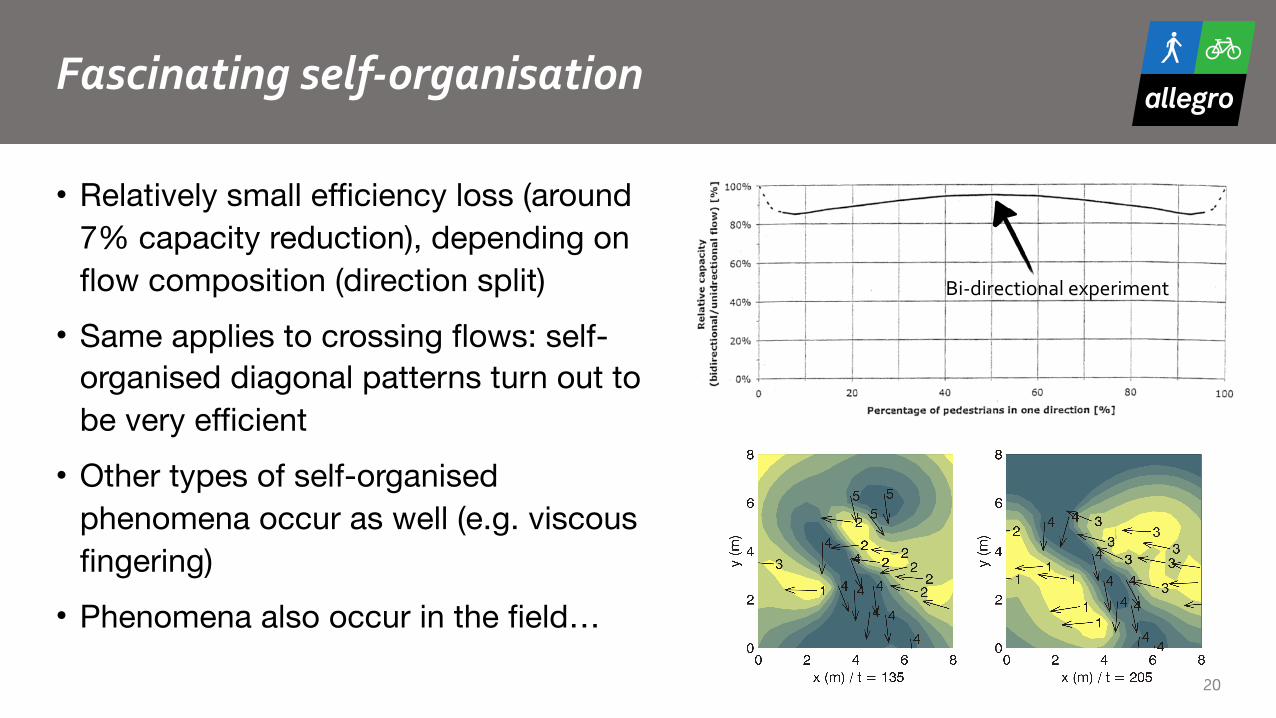
• Relatively small efficiency loss (around 7% capacity reduction), depending on flow composition (direction split)
• Same applies to crossing flows: self-organised diagonal patterns turn out to be very efficient
• Other types of self-organised phenomena occur as well (e.g. viscous fingering)
• Phenomena also occur in the field…
20
Bi-directionalexperiment

Studyingself-organisationduringrockconcertLowlands…
Pedestrianflowoperations…
So with this wonderful
self-organisation, why do
we need to worry about
crowds at all?
22
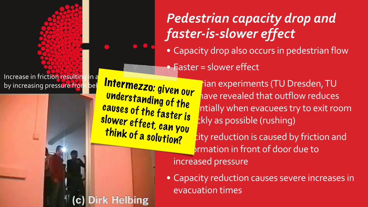
Increaseinfrictionresultinginarcformationbyincreasingpressurefrombehind(force-
Pedestriancapacitydropandfaster-is-slowereffect• Capacitydropalsooccursinpedestrianflow
• Faster=slowereffect
• Pedestrianexperiments(TUDresden,TUDelft)haverevealedthatoutflowreducessubstantiallywhenevacueestrytoexitroomasquicklyaspossible(rushing)
• Capacityreductioniscausedbyfrictionandarc-formationinfrontofdoorduetoincreasedpressure
• Capacityreductioncausessevereincreasesinevacuationtimes
Intermezzo: given our understanding of the causes of the faster is slower effect, can you think of a solution?
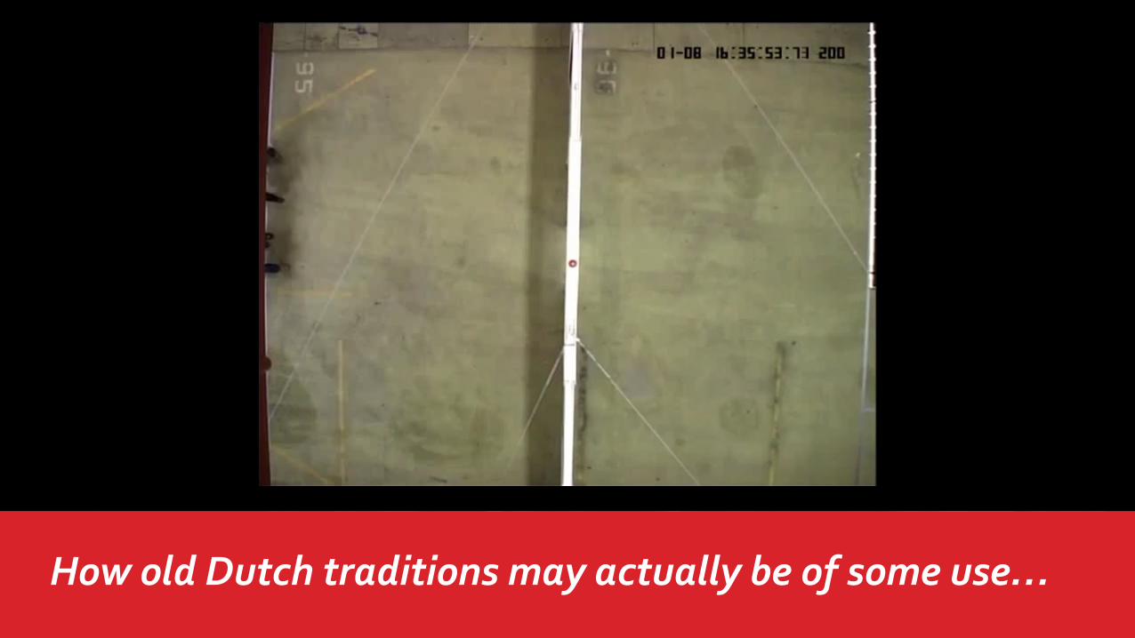
HowoldDutchtraditionsmayactuallybeofsomeuse…
24
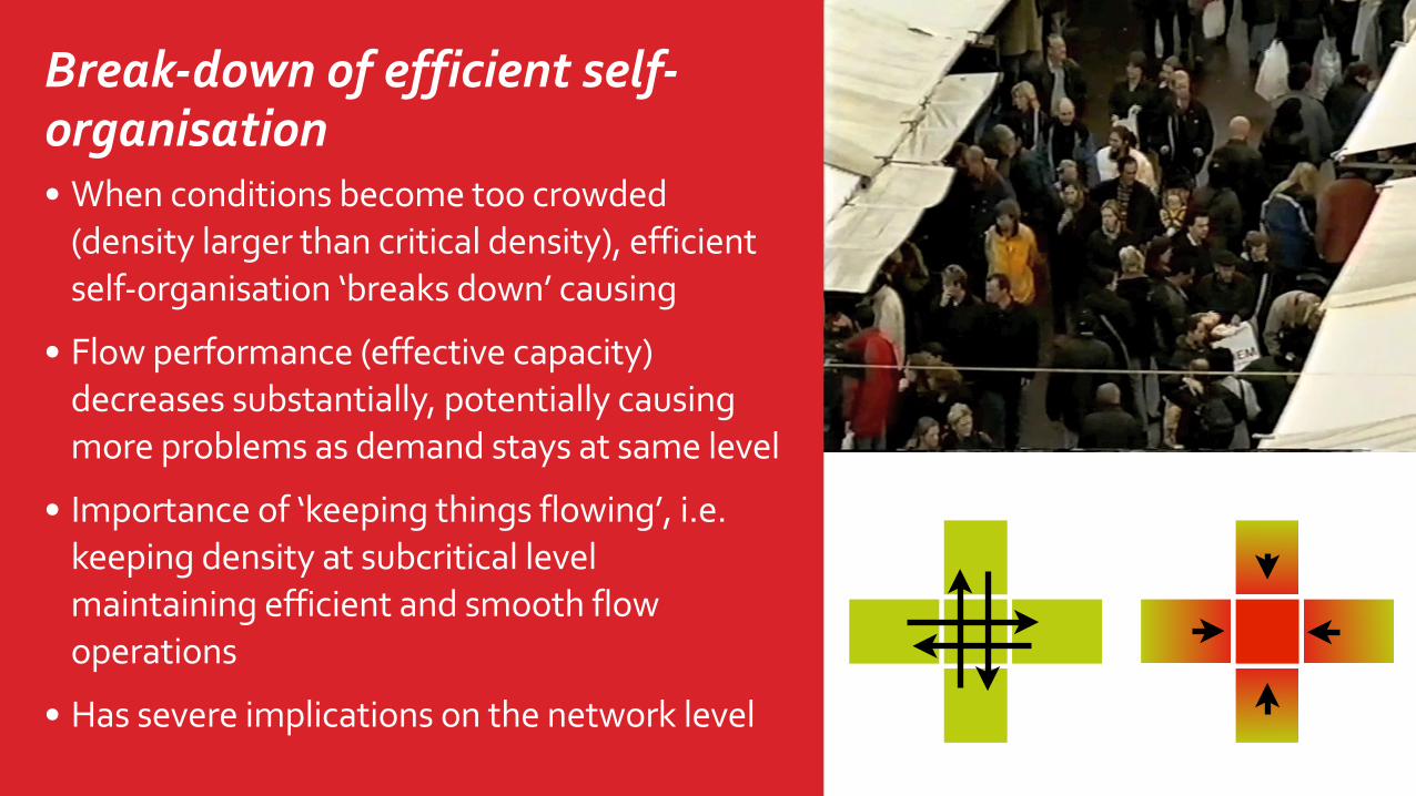
Break-downofefficientself-organisation• Whenconditionsbecometoocrowded(densitylargerthancriticaldensity),efficientself-organisation‘breaksdown’causing
• Flowperformance(effectivecapacity)decreasessubstantially,potentiallycausingmoreproblemsasdemandstaysatsamelevel
• Importanceof‘keepingthingsflowing’,i.e.keepingdensityatsubcriticallevelmaintainingefficientandsmoothflowoperations
• Hassevereimplicationsonthenetworklevel
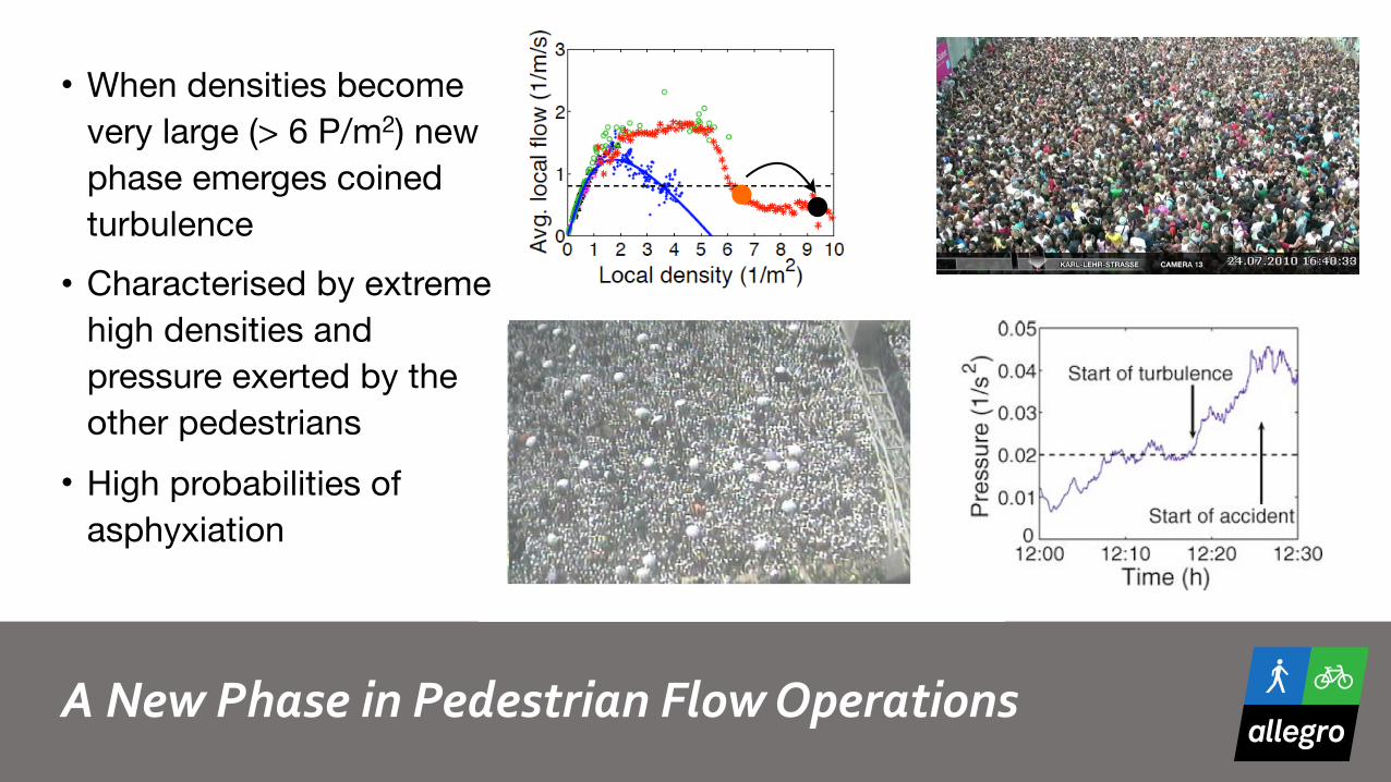
ANewPhaseinPedestrianFlowOperations
• When densities become very large (> 6 P/m2) new phase emerges coined turbulence
• Characterised by extreme high densities and pressure exerted by the other pedestrians
• High probabilities of asphyxiation
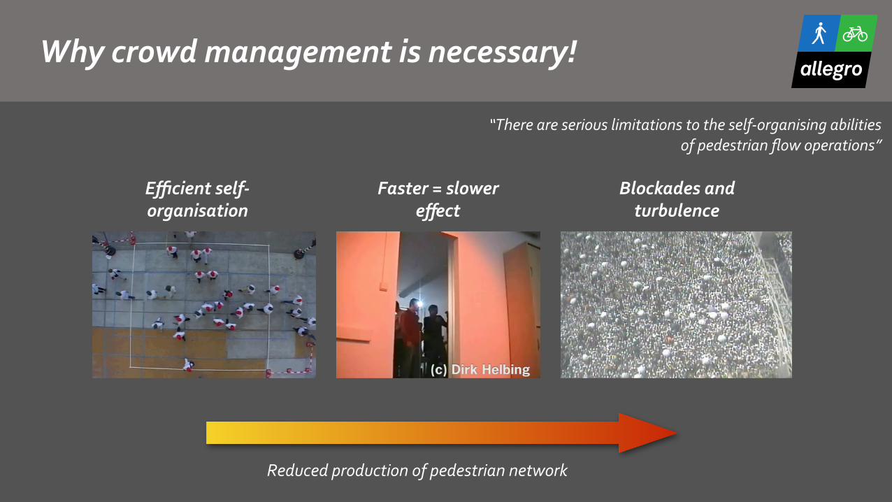
Whycrowdmanagementisnecessary!
Efficientself-organisation
Faster=slowereffect
Blockadesandturbulence
“Thereareseriouslimitationstotheself-organisingabilities ofpedestrianflowoperations”
Reducedproductionofpedestriannetwork
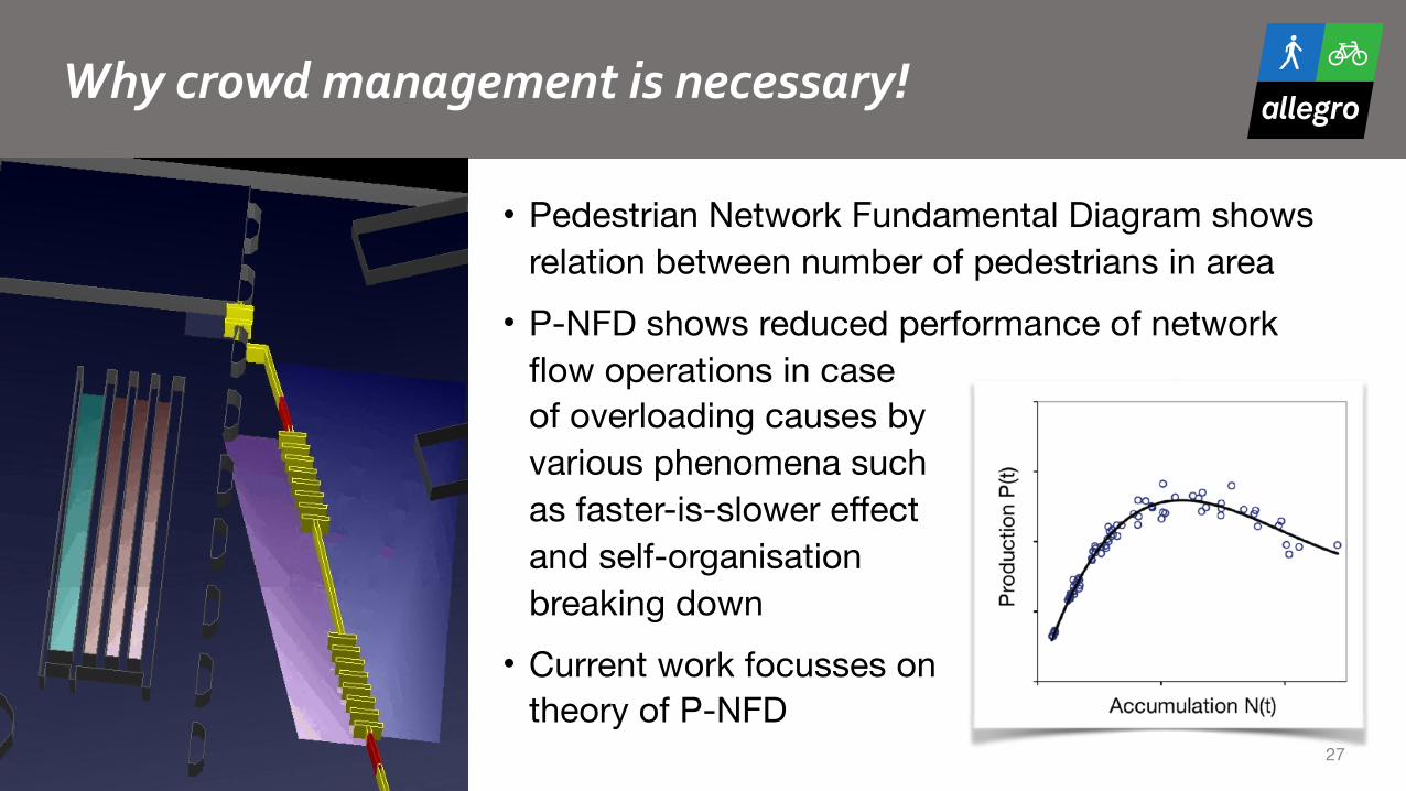
Whycrowdmanagementisnecessary!
• Pedestrian Network Fundamental Diagram shows relation between number of pedestrians in area
• P-NFD shows reduced performance of network flow operations in case of overloading causes by various phenomena such as faster-is-slower effect and self-organisation breaking down
• Current work focusses on theory of P-NFD
27
28
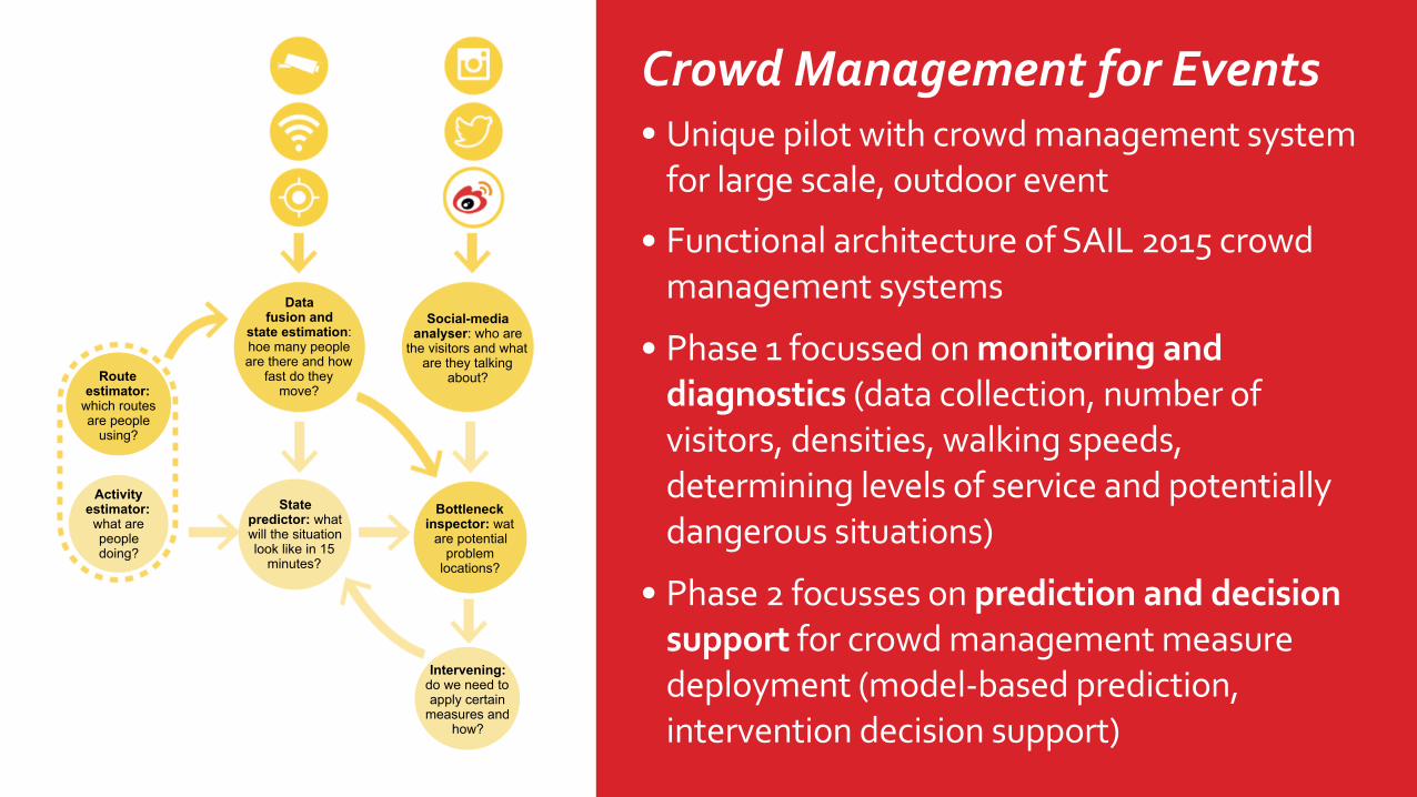
CrowdManagementforEvents• Uniquepilotwithcrowdmanagementsystemforlargescale,outdoorevent
• FunctionalarchitectureofSAIL2015crowdmanagementsystems
• Phase1focussedonmonitoringanddiagnostics(datacollection,numberofvisitors,densities,walkingspeeds,determininglevelsofserviceandpotentiallydangeroussituations)
• Phase2focussesonpredictionanddecisionsupportforcrowdmanagementmeasuredeployment(model-basedprediction,interventiondecisionsupport)
Data fusion and
state estimation: hoe many people are there and how
fast do they move?
Social-media analyser: who are
the visitors and what are they talking
about?
Bottleneck inspector: wat
are potential problem
locations?
State predictor: what will the situation look like in 15
minutes?
Route estimator:
which routes are people
using?
Activity estimator: what are people doing?
Intervening: do we need to apply certain
measures and how?
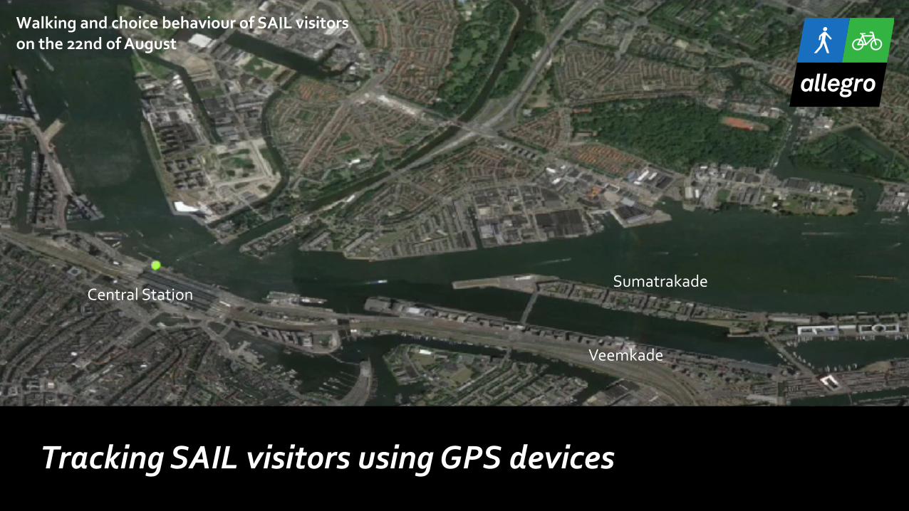
TrackingSAILvisitorsusingGPSdevices
CentralStation
WalkingandchoicebehaviourofSAILvisitors onthe22ndofAugust
Veemkade
Sumatrakade

Exampledashboardoutcomes
• Newly developed algorithm to distinguish between occupancy time and walking time
• Other examples show volumes and OD flows • Results used for real-time intervention, but also for
planning of SAIL 2020 (simulation studies)0
5
10
15
20
25
30
11 12 13 14 15 16 17 18 19
Verblijf) en+looptijden+Veemkade
verblijftijd looptijd
1988
1881
4760
4958
2202
1435
6172
59994765 4761
4508
3806
3315
2509
17523774
4061
2629
13592654
21391211
1439
2209
1638
2581
311024653067
2760
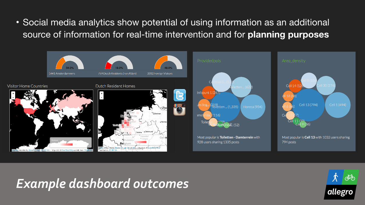
Exampledashboardoutcomes
• Social media analytics show potential of using information as an additional source of information for real-time intervention and for planning purposes
32
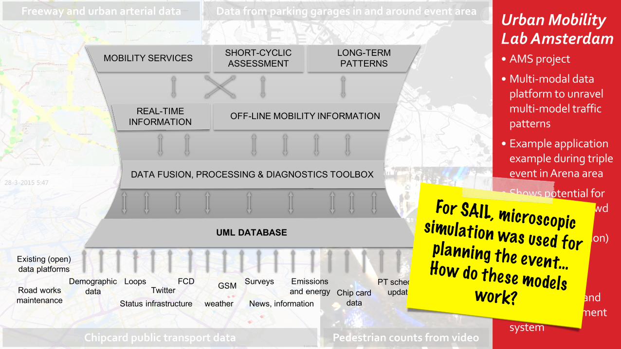
UrbanMobilityLabAmsterdam• AMSproject
• Multi-modaldataplatformtounravelmulti-modeltrafficpatterns
• ExampleapplicationexampleduringtripleeventinArenaarea
• ShowspotentialforuseofUMLincrowdmanagement(demandprediction)andinmorecomprehensivemulti-modaltransportationandtrafficmanagementsystem
Freewayandurbanarterialdata Datafromparkinggaragesinandaroundeventarea
Chipcardpublictransportdata Pedestriancountsfromvideo
Loops FCD GSM Surveys Emissionsand energy Chip card
dataTwitterRoad works
maintenance
PT schedules updates
Events, incidents, accidentsDemographic
data
REAL-TIME INFORMATION OFF-LINE MOBILITY INFORMATION
MOBILITY SERVICES SHORT-CYCLIC ASSESSMENT
LONG-TERMPATTERNS
UML DATABASE
Status infrastructure weather News, informationVecom data
Existing (open) data platforms
DATA FUSION, PROCESSING & DIAGNOSTICS TOOLBOX
For SAIL, microscopic simulation was used for planning the event… How do these models work?
Modellingforplanning
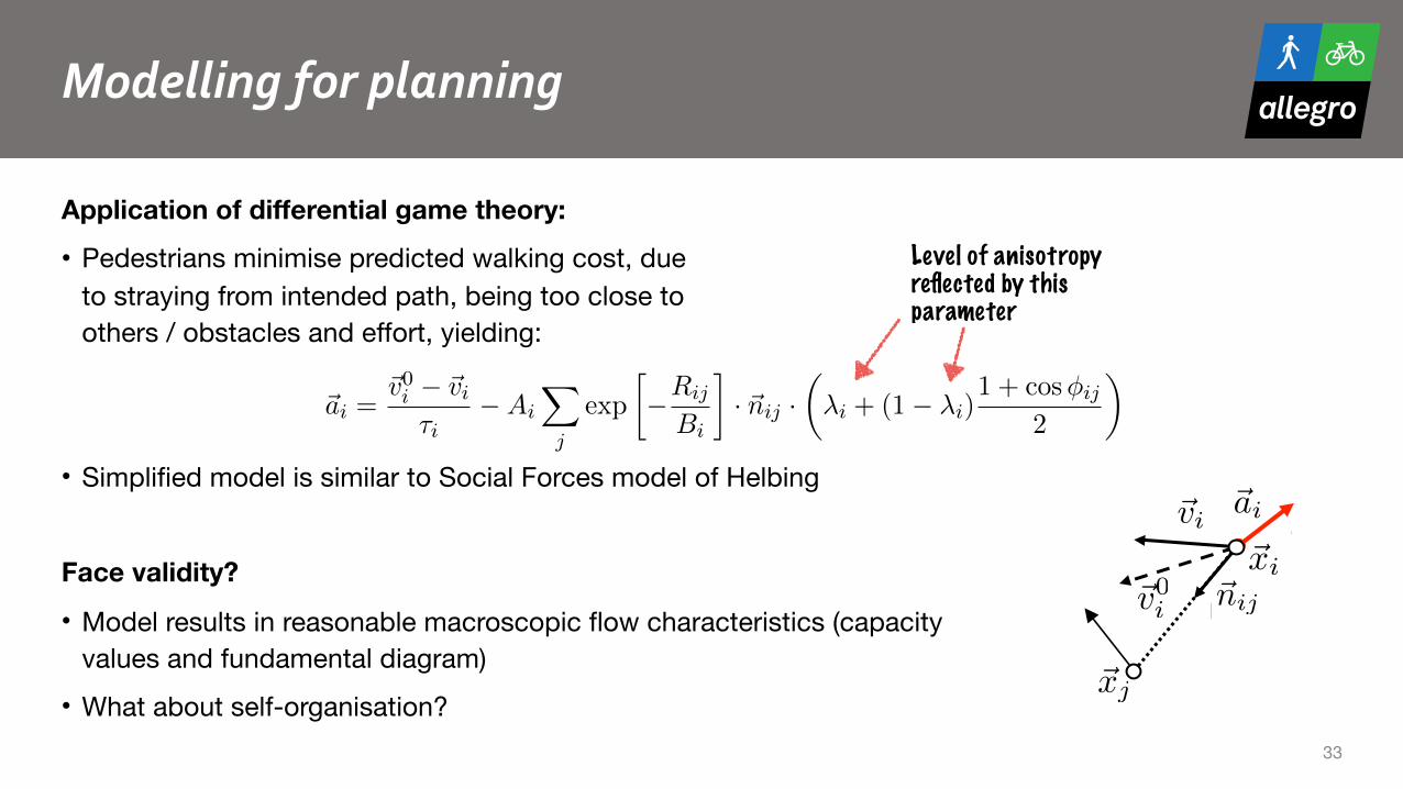
Application of differential game theory: • Pedestrians minimise predicted walking cost, due
to straying from intended path, being too close to others / obstacles and effort, yielding:
• Simplified model is similar to Social Forces model of Helbing
Face validity?
• Model results in reasonable macroscopic flow characteristics (capacity values and fundamental diagram)
• What about self-organisation? 33
FROM MICROSCOPIC TO MACROSCOPIC INTERACTIONMODELING
SERGE P. HOOGENDOORN
1. Introduction
This memo aims at connecting the microscopic modelling principles underlying thesocial-forces model to identify a macroscopic flow model capturing interactions amongstpedestrians. To this end, we use the anisotropic version of the social-forces model pre-sented by Helbing to derive equilibrium relations for the speed and the direction, giventhe desired walking speed and direction, and the speed and direction changes due tointeractions.
2. Microscopic foundations
We start with the anisotropic model of Helbing that describes the acceleration ofpedestrian i as influence by opponents j:
(1) ~ai
=~v0i
� ~vi
⌧i
�Ai
X
j
exp
�R
ij
Bi
�· ~n
ij
·✓�i
+ (1� �i
)1 + cos�
ij
2
◆
where Rij
denotes the distance between pedestrians i and j, ~nij
the unit vector pointingfrom pedestrian i to j; �
ij
denotes the angle between the direction of i and the postionof j; ~v
i
denotes the velocity. The other terms are all parameters of the model, that willbe introduced later.
In assuming equilibrium conditions, we generally have ~ai
= 0. The speed / directionfor which this occurs is given by:
(2) ~vi
= ~v0i
� ⌧i
Ai
X
j
exp
�R
ij
Bi
�· ~n
ij
·✓�i
+ (1� �i
)1 + cos�
ij
2
◆
Let us now make the transition to macroscopic interaction modelling. Let ⇢(t, ~x)denote the density, to be interpreted as the probability that a pedestrian is present onlocation ~x at time instant t. Let us assume that all parameters are the same for allpedestrian in the flow, e.g. ⌧
i
= ⌧ . We then get:(3)
~v = ~v0(~x)� ⌧A
ZZ
~y2⌦(~x)
exp
✓� ||~y � ~x||
B
◆✓�+ (1� �)
1 + cos�xy
(~v)
2
◆~y � ~x
||~y � ~x||⇢(t, ~y)d~y
Here, ⌦(~x) denotes the area around the considered point ~x for which we determine theinteractions. Note that:
(4) cos�xy
(~v) =~v
||~v|| ·~y � ~x
||~y � ~x||1
Level of anisotropy reflected by this parameter
~vi
~v0i
~ai
~nij
~xi
~xj
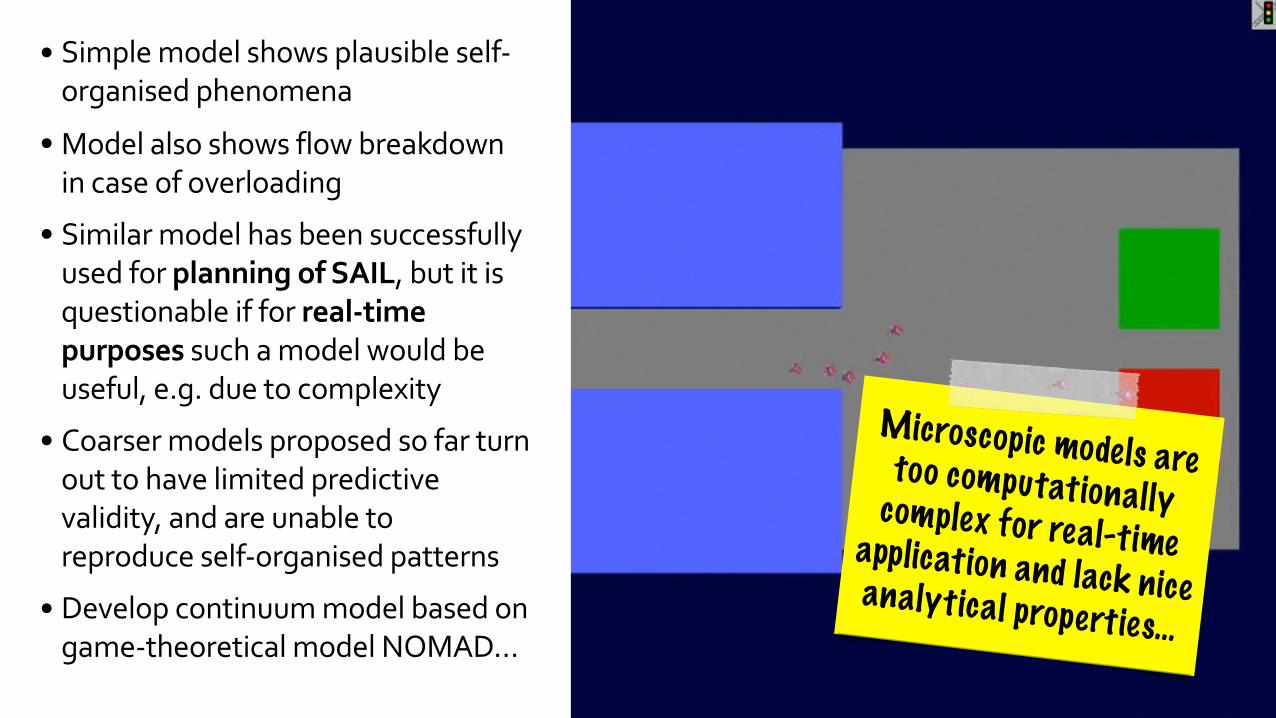
• Simplemodelshowsplausibleself-organisedphenomena
• Modelalsoshowsflowbreakdownincaseofoverloading
• SimilarmodelhasbeensuccessfullyusedforplanningofSAIL,butitisquestionableifforreal-timepurposessuchamodelwouldbeuseful,e.g.duetocomplexity
• Coarsermodelsproposedsofarturnouttohavelimitedpredictivevalidity,andareunabletoreproduceself-organisedpatterns
• Developcontinuummodelbasedongame-theoreticalmodelNOMAD…
Microscopic models are too computationally complex for real-time application and lack nice analytical properties…

Modellingforplanningandreal-timepredictions
• NOMAD / Social-forces model as starting point:
• Equilibrium relation stemming from model (ai = 0):
• Interpret density as the ‘probability’ of a pedestrian being present, which gives a macroscopic equilibrium relation (expected velocity), which equals:
• Combine with conservation of pedestrian equation yields complete model, but numerical integration is computationally very intensive
35
FROM MICROSCOPIC TO MACROSCOPIC INTERACTIONMODELING
SERGE P. HOOGENDOORN
1. Introduction
This memo aims at connecting the microscopic modelling principles underlying thesocial-forces model to identify a macroscopic flow model capturing interactions amongstpedestrians. To this end, we use the anisotropic version of the social-forces model pre-sented by Helbing to derive equilibrium relations for the speed and the direction, giventhe desired walking speed and direction, and the speed and direction changes due tointeractions.
2. Microscopic foundations
We start with the anisotropic model of Helbing that describes the acceleration ofpedestrian i as influence by opponents j:
(1) ~ai
=~v0i
� ~vi
⌧i
�Ai
X
j
exp
�R
ij
Bi
�· ~n
ij
·✓�i
+ (1� �i
)1 + cos�
ij
2
◆
where Rij
denotes the distance between pedestrians i and j, ~nij
the unit vector pointingfrom pedestrian i to j; �
ij
denotes the angle between the direction of i and the postionof j; ~v
i
denotes the velocity. The other terms are all parameters of the model, that willbe introduced later.
In assuming equilibrium conditions, we generally have ~ai
= 0. The speed / directionfor which this occurs is given by:
(2) ~vi
= ~v0i
� ⌧i
Ai
X
j
exp
�R
ij
Bi
�· ~n
ij
·✓�i
+ (1� �i
)1 + cos�
ij
2
◆
Let us now make the transition to macroscopic interaction modelling. Let ⇢(t, ~x)denote the density, to be interpreted as the probability that a pedestrian is present onlocation ~x at time instant t. Let us assume that all parameters are the same for allpedestrian in the flow, e.g. ⌧
i
= ⌧ . We then get:(3)
~v = ~v0(~x)� ⌧A
ZZ
~y2⌦(~x)
exp
✓� ||~y � ~x||
B
◆✓�+ (1� �)
1 + cos�xy
(~v)
2
◆~y � ~x
||~y � ~x||⇢(t, ~y)d~y
Here, ⌦(~x) denotes the area around the considered point ~x for which we determine theinteractions. Note that:
(4) cos�xy
(~v) =~v
||~v|| ·~y � ~x
||~y � ~x||1

Modellingforplanningandreal-timepredictions
• Taylor series approximation: yields a closed-form expression for the equilibrium velocity , which is given by the equilibrium speed and direction:
with:• Check behaviour of model by looking at isotropic flow ( ) and homogeneous flow
conditions ( ) • Include conservation of pedestrian relation gives a complete model…
36
2 SERGE P. HOOGENDOORN
From this expression, we can find both the equilibrium speed and the equilibrium direc-tion, which in turn can be used in the macroscopic model.
We can think of approximating this expression, by using the following linear approx-imation of the density around ~x:
(5) ⇢(t, ~y) = ⇢(t, ~x) + (~y � ~x) ·r⇢(t, ~x) +O(||~y � ~x||2)
Using this expression into Eq. (3) yields:
(6) ~v = ~v0(~x)� ~↵(~v)⇢(t, ~x)� �(~v)r⇢(t, ~x)
with ↵(~v) and �(~v) defined respectively by:
(7) ~↵(~v) = ⌧A
ZZ
~y2⌦(~x)
exp
✓� ||~y � ~x||
B
◆✓�+ (1� �)
1 + cos�xy
(~v)
2
◆~y � ~x
||~y � ~x||d~y
and
(8) �(~v) = ⌧A
ZZ
~y2⌦(~x)
exp
✓� ||~y � ~x||
B
◆✓�+ (1� �)
1 + cos�xy
(~v)
2
◆||~y � ~x||d~y
To investigate the behaviour of these integrals, we have numerically approximatedthem. To this end, we have chosen ~v( ) = V · (cos , sin ), for = 0...2⇡. Fig. 1 showsthe results from this approximation.
0 1 2 3 4 5 6 7−0.25
−0.2
−0.15
−0.1
−0.05
0
0.05
0.1
0.15
0.2
0.25
angle
valu
e
α
1
α2
β
Figure 1. Numerical approximation of ~↵(~v) and �(~v).
For the figure, we can clearly see that � is independent on ~v, i.e.
(9) �(~v) = �0
FROM MICROSCOPIC TO MACROSCOPIC INTERACTION MODELING 3
Furthermore, we see that for ~↵, we find:
(10) ~↵(~v) = ↵0 ·~v
||~v||
(Can we determine this directly from the integrals?)From Eq. (6), with ~v = ~e · V we can derive:
(11) V = ||~v0 � �0 ·r⇢||� ↵0⇢
and
(12) ~e =~v0 � �0 ·r⇢
V + ↵0⇢=
~v0 � �0 ·r⇢
||~v0 � �0 ·r⇢||
Note that the direction does not depend on ↵0, which implies that the magnitude ofthe density itself has no e↵ect on the direction, while the gradient of the density does
influence the direction.
2.1. Homogeneous flow conditions. Note that in case of homogeneous conditions,i.e. r⇢ = ~0, Eq. (11) simplifies to
(13) V = ||~v0||� ↵0⇢ = V 0 � ↵0⇢
i.e. we see a linear relation between speed and density. For the direction ~e, we then get:
(14) ~e =~v0
V + ↵0⇢= ~e0
In other words, in homogeneous density conditions the direction of the pedestrians isequal to the desired direction.
2.2. Isotropic walking behaviour. Let us also note that in case � = 1 (isotropicflow), and assuming that ⌦ is symmetric around ~x, we get:
(15) ~↵(~v) = ⌧A
ZZ
~y2⌦(~x)
exp
✓� ||~y � ~x||
B
◆~y � ~x
||~y � ~x||d~y = ~0
which means ↵0 = 0. In this case, we have:
(16) V = ||~v0 � �0 ·r⇢||
This expression shows that in this case, the speed is only dependent on the densitygradient. If a pedestrian walks into a region in which the density is increasing, the speedwill be less than the desired speed; and vice versa. Also note that in case of homogenousconditions, the speed will be constant and equal to the free speed. Note that this isconsistent with the results from Hoogendoorn, ISTTT-2003.
For the direction, we find:
(17) ~e =~v0 � �0 ·r⇢
||~v0 � �0 ·r⇢||
α 0 = πτAB2 (1− λ) and β0 = 2πτAB3(1+ λ)
4.1. Analysis of model properties
Let us first take a look at expressions (14) and (15) describing the equilibrium290
speed and direction. Notice first that the direction does not depend on ↵0, which
implies that the magnitude of the density itself has no e↵ect, and that only the
gradient of the density does influence the direction. We will now discuss some
other properties, first by considering a homogeneous flow (r⇢ = ~0), and then
by considering an isotropic flow (� = 1) and an anisotropic flow (� = 0).295
4.1.1. Homogeneous flow conditions
Note that in case of homogeneous conditions, i.e. r⇢ = ~0, Eq. (14) simplifies
to
V = ||~v0||� ↵0⇢ = V 0 � ↵0⇢ (16)
i.e. we see a linear relation between speed and density. The term ↵0 � 0
describes the reduction of the speed with increasing density.300
For the direction ~e, we then get:
~e =~v0
||~v0|| = ~e0 (17)
In other words, in homogeneous density conditions the direction of the pedestri-
ans is equal to the desired direction. Clearly, the gradient of the density yields
pedestrians to divert from their desired direction.
Looking further at the expressions for ↵0 and �0, we can see the influence of305
the various parameters on their size; ↵0 scales linearly with A and ⌧ , meaning
that the influence of the density on the speed increases with increasing values
of A and ⌧ . At the same time, larger values for B imply a reduction of the
influence of the density. Needs to be revised!
The same can be concluded for the influence of the gradient: we see linear310
scaling for A and ⌧ , and reducing influence with larger values of B. This holds
for the equilibrium speed and direction. Needs to be revised!
13
!v = !e ⋅V
37
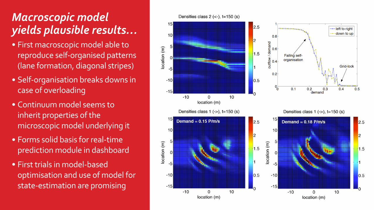
Macroscopicmodelyieldsplausibleresults…• Firstmacroscopicmodelabletoreproduceself-organisedpatterns(laneformation,diagonalstripes)
• Self-organisationbreaksdownsincaseofoverloading
• Continuummodelseemstoinheritpropertiesofthemicroscopicmodelunderlyingit
• Formssolidbasisforreal-timepredictionmoduleindashboard
• Firsttrialsinmodel-basedoptimisationanduseofmodelforstate-estimationarepromising

38
Prevent blockades by separating flows in different directions / use of reservoirs
Distribute traffic over available infrastructure by means of guidance or information provision
Increase throughput in particular at pinch points in the design…
Limit the inflow (gating) ensuring that number of pedestrians stays below critical value!
Principlesofcrowdmanagement• Developingcrowdmanagementinterventionsusinginsightsinpedestrianflowcharacteristics
• Goldenrules(solutiondirections)providedirectionsinwhichtothinkwhenconsideringcrowdmanagementoptions
ApplicationexampleduringAlMatafdesign

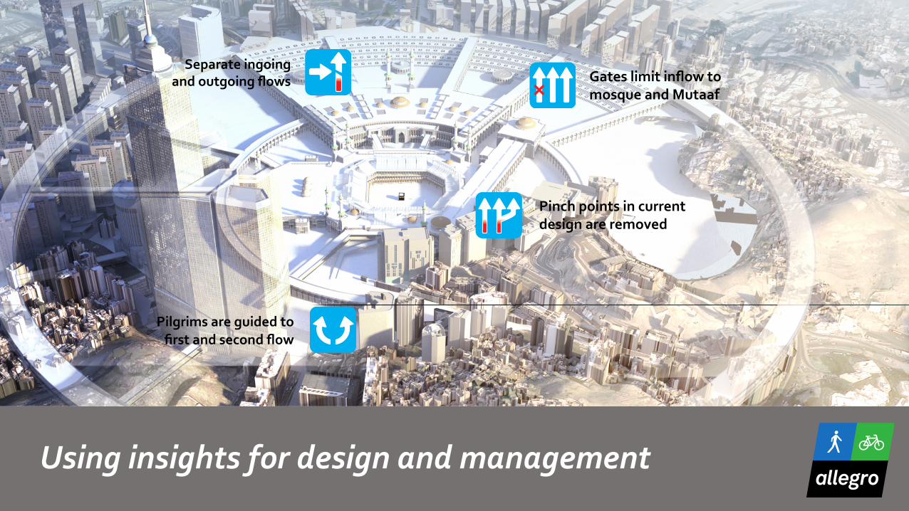
Usinginsightsfordesignandmanagement
Separateingoingandoutgoingflows Gateslimitinflowto
mosqueandMutaaf
Pilgrimsareguidedtofirstandsecondflow
Pinchpointsincurrentdesignareremoved
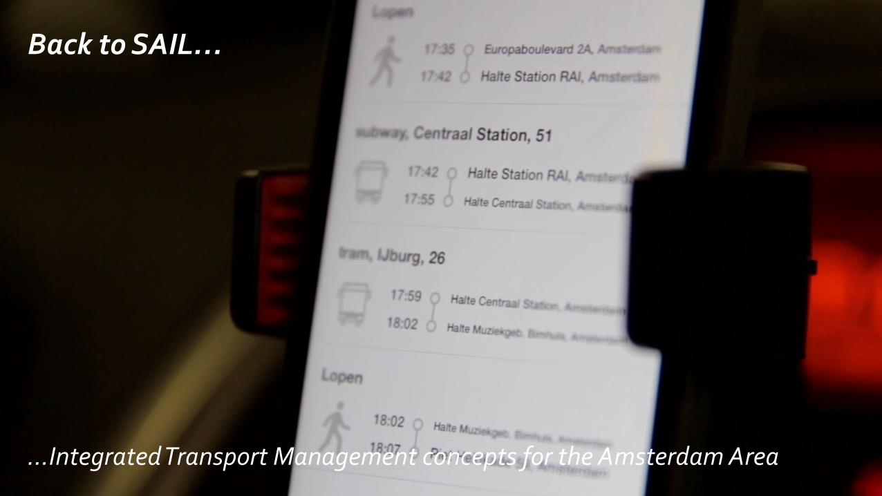
BacktoSAIL…
…IntegratedTransportManagementconceptsfortheAmsterdamArea

42
PracticalPilotAmsterdam• UniquepracticalpilotINM
• FullyautomatedcoordinateddeploymentoftrafficmanagementmeasurestoimprovethroughputonA10West
• Firstphasesuccessful,secondphasecurrentlyrunning
• Towardstrafficmanagement2.0:integratingroad-sideandin-cartrafficmeasuresforstateestimation(datafusion)andactuation(anticipatorytrafficmanagement)
• WorkingonMelbournepilot(HaiLeVu,Swinburne)
http://www.ipam.ucla.edu/programs/workshops/workshop-iv-decision-support-for-traffic/?tab=schedule
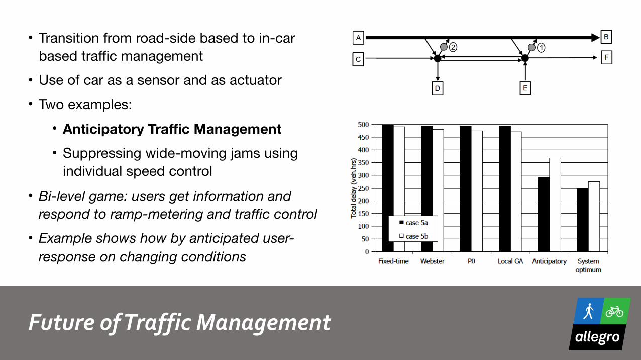
FutureofTrafficManagement
• Transition from road-side based to in-car based traffic management
• Use of car as a sensor and as actuator• Two examples:
• Anticipatory Traffic Management • Suppressing wide-moving jams using
individual speed control• Bi-level game: users get information and
respond to ramp-metering and traffic control • Example shows how by anticipated user-
response on changing conditions
Start
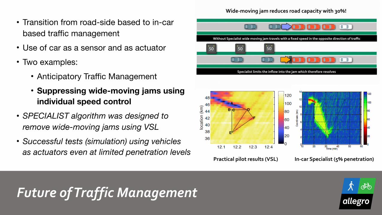
FutureofTrafficManagement
• Transition from road-side based to in-car based traffic management
• Use of car as a sensor and as actuator• Two examples:
• Anticipatory Traffic Management• Suppressing wide-moving jams using
individual speed control • SPECIALIST algorithm was designed to
remove wide-moving jams using VSL • Successful tests (simulation) using vehicles
as actuators even at limited penetration levels
Start
Practicalpilotresults(VSL) In-carSpecialist(5%penetration)
Wide-movingjamreducesroadcapacitywith30%!
WithoutSpecialistwidemovingjamtravelswithafixedspeedintheoppositedirectionoftraffic
Specialistlimitstheinflowintothejamwhichthereforeresolves

Closingremarks
• Urbanisation yields both new challenges and new opportunities for sustainable transport and accessibility (e.g. via seamless multi-modal transport) and motivates focus on Intelligent Urban Mobility under umbrella of Smart City projects such as AMS
• Increasing share of active modes can have major impacts on accessibility, liveability and health!
• Focus on keeping urban pedestrian and bike safety and comfort at high levels by means active mode traffic management (e.g. crowd management) offers unprecedented scientific challenges in data collection, modelling and simulation, and control and management!
• Co-existence with other future transport concepts such as self-driving vehicles will be a challenge as will, in particular in dense cities such as Amsterdam
45
Moreinformation?
• Hoogendoorn, S.P., van Wageningen-Kessels, F., Daamen, W., Duives, D.C., Sarvi, M. Continuum theory for pedestrian traffic flow: Local route choice modelling and its implications (2015) Transportation Research Part C: Emerging Technologies, 59, pp. 183-197.
• Van Wageningen-Kessels, F., Leclercq, L., Daamen, W., Hoogendoorn, S.P. The Lagrangian coordinate system and what it means for two-dimensional crowd flow models (2016) Physica A: Statistical Mechanics and its Applications, 443, pp. 272-285.
• Hoogendoorn, S.P., Van Wageningen-Kessels, F.L.M., Daamen, W., Duives, D.C. Continuum modelling of pedestrian flows: From microscopic principles to self-organised macroscopic phenomena (2014) Physica A: Statistical Mechanics and its Applications, 416, pp. 684-694.
• Taale, H., Hoogendoorn, S.P. A framework for real-time integrated and anticipatory traffic management (2013) IEEE Conference on Intelligent Transportation Systems, Proceedings, ITSC, art. no. 6728272, pp. 449-454.
• Hoogendoorn, S.P., Landman, R., Van Kooten, J., Schreuder, M. Integrated Network Management Amsterdam: Control approach and test results (2013) IEEE Conference on Intelligent Transportation Systems, Proceedings, ITSC, art. no. 6728276, pp. 474-479.
• Le, T., Vu, H.L., Nazarathy, Y., Vo, Q.B., Hoogendoorn, S. Linear-quadratic model predictive control for urban traffic networks (2013) Transportation Research Part C: Emerging Technologies, 36, pp. 498-512. 46