unm advanced data analysis 2 notes - statacumen.com

Chapter 17

Classification

Contents17.1 Discriminant analysis . . . . . . . . . . . . . . . . . . . . . 532

17.2 Classification using Mahalanobis distance . . . . . . . . . 535

17.3 Evaluating the Accuracy of a Classification Rule . . . . . 538

17.4 Example: Carapace classification and error . . . . . . . . 540

17.5 Example: Fisher’s Iris Data cross-validation . . . . . . . . 548

17.5.1 Stepwise variable selection for classification . . . . . . . . . 558

17.6 Example: Analysis of Admissions Data . . . . . . . . . . . 561

17.6.1 Further Analysis of the Admissions Data . . . . . . . . . . 563

17.6.2 Classification Using Unequal Prior Probabilities . . . . . . 568

17.6.3 Classification With Unequal Covariance Matrices, QDA . . 574

17.1 Discriminant analysis

A goal with discriminant analysis might be to classify individuals of unknown

origin into one of several known groups. How should this be done? Recall

our example where two subspecies of an insect are compared on two external

features. The discriminant analysis gives one discriminant function (CAN1) for

distinguishing the subspecies. It makes sense to use CAN1 to classify insects

Prof. Erik B. Erhardt

17.1: Discriminant analysis 533

because CAN1 is the best (linear) combination of the features to distinguish

between subspecies.

Given the score on CAN1 for each insect to be classified, assign insects to

the sub-species that they most resemble. Similarity is measured by the distance

on CAN1 to the average CAN1 scores for the two subspecies, identified by X’s

on the plot.

To classify using r discriminant functions, compute the average response on

CAN1, . . . , CANr in each sample. Then compute the canonical discriminant

function scores for each individual to be classified. Each observation is classified

into the group it is closest to, as measured by the distance from the observation

in r-space to the sample mean vector on the canonical variables. How do you

measure distance in r-space?

UNM, Stat 428/528 ADA2

534 Ch 17: Classification

The plot below illustrates the idea with the r = 2 discriminant functions

in Fisher’s iris data: Obs 1 is classified as Versicolor and Obs 2 is classified as

Setosa.## Error in select(., Species, Can1, Can2, Can1SE, Can2SE): unused arguments (Species, Can1, Can2, Can1SE, Can2SE)## Error in eval(expr, envir, enclos): object ’Can means’ not found## Error in fortify(data): object ’Can means’ not found## Error in fortify(data): object ’Can means’ not found

●

●

●

●

●

●

●

●

●●

●

●

●

●

●

●

●

●

●●

●

●

●

●

●

●

●

●●

●

●

●

●

●

●

●

●●

●

●

●

●

●

●●

●

●

●

●

●

obs 1

obs 2

−2

0

2

−10 −5 0 5 10Can1

Can

2

Species

● setosa

versicolor

virginica


17.2: Classification using Mahalanobis distance 535

17.2 Classification using Mahalanobis dis-tance

Classification using discrimination is based on the original features and not

the canonical discriminant function scores. Although a linear classification rule

is identical to the method I just outlined, the equivalence is not obvious. I will

discuss the method without justifying the equivalence.

Suppose p features X = (X1, X2, . . . , Xp)′ are used to discriminate among

the k groups. Let X̄i = (X̄i1, X̄i2, . . . , X̄ip)′ be the vector of mean responses

for the ith sample, and let Si be the p-by-p variance-covariance matrix for the

ith sample. The pooled variance-covariance matrix is given by

S =(n1 − 1)S1 + (n2 − 1)S2 + · · · + (nk − 1)Sk

n− k,

where the nis are the group sample sizes and n = n1 + n2 + · · · + nk is the

total sample size.

The classification rules below can be defined using either the Mahalanobis

generalized squared distance or in terms of a probability model. I will

describe each, starting with the Mahalanobis or M -distance.

The M -distance from an observation X to (the center of) the ith sample is

D2i (X) = (X − X̄i)

′S−1(X − X̄i),

where (X−X̄i)′ is the transpose of the column vector (X−X̄i), and S−1 is the

matrix inverse of S. Note that if S is the identity matrix (a matrix with 1s on

the diagonal and 0s on the off-diagonals), then this is the Euclidean distance.

Given the M -distance from X to each sample, classify X into the group which

has the minimum M -distance.

The M -distance is an elliptical distance measure that accounts for corre-

lation between features, and adjusts for different scales by standardizing the

features to have unit variance. The picture below (left) highlights the idea

when p = 2. All of the points on a given ellipse are the same M -distance



to the center (X̄1, X̄2)′. As the ellipse expands, the M -distance to the center

increases.

0 2 4 6

24

68

X1

X2

X1, X2

= (3,5)

Corr X1, X2 > 0

0 5 10 15−

20

24

68

X1

X2

Group 1

Group 2

Group 3

obs 1

obs 2

obs 3

To see how classification works, suppose you have three groups and two

features, as in the plot above (right). Observations 1 is closest in M -distance

to the center of group 3. Observation 2 is closest to group 1. Thus, classify

observations 1 and 2 into groups 3 and 1, respectively. Observation 3 is closest

to the center of group 2 in terms of the standard Euclidean (walking) distance.

However, observation 3 is more similar to data in group 1 than it is to either of

the other groups. The M -distance from observation 3 to group 1 is substantially

smaller than the M -distances to either group 2 or 3. The M -distance accounts

for the elliptical cloud of data within each group, which reflects the correlation

between the two features. Thus, you would classify observation 3 into group 1.

The M -distance from the ith group to the jth group is the M -distance

between the centers of the groups:

D2(i, j) = D2(j, i) = (X̄i − X̄j)′S−1(X̄i − X̄j).

Larger values suggest relatively better potential for discrimination between

groups. In the plot above, D2(1, 2) < D2(1, 3) which implies that it should

be easier to distinguish between groups 1 and 3 than groups 1 and 2.


17.2: Classification using Mahalanobis distance 537

M -distance classification is equivalent to classification based on a probability

model that assumes the samples are independently selected from multivariate

normal populations with identical covariance matrices. This assumption is

consistent with the plot above where the data points form elliptical clouds with

similar orientations and spreads across samples. Suppose you can assume a

priori (without looking at the data for the individual that you wish to classify)

that a randomly selected individual from the combined population (i.e.,

merge all sub-populations) is equally likely to be from any group:

PRIORj ≡ Pr(observation is from group j) =1

k,

where k is the number of groups. Then, given the observed features X for an

individual

Pr(j|X) ≡ Pr(observation is from group j given X)

=exp{−0.5D2

j (X)}∑k exp{−0.5D2

k(X)}.

To be precise, I will note that Pr(j|X) is unknown, and the expression for

Pr(j|X) is an estimate based on the data.

The group with the largest posterior probability Pr(j|X) is the group

into which X is classified. Maximizing Pr(j|X) across groups is equivalent to

minimizing the M -distance D2j (X) across groups, so the two classification rules

are equivalent.



17.3 Evaluating the Accuracy of a Classifi-cation Rule

The misclassification rate, or the expected proportion of misclassified ob-

servations, is a good yardstick to gauge a classification rule. Better rules have

smaller misclassification rates, but there is no universal cutoff for what is con-

sidered good in a given problem. You should judge a classification rule relative

to the current standards in your field for “good classification”.

Resubstitution evaluates the misclassification rate using the data from

which the classification rule is constructed. The resubstitution estimate of the

error rate is optimistic (too small). A greater percentage of misclassifications is

expected when the rule is used on new data, or on data from which the rule is

not constructed.

Cross-validation is a better way to estimate the misclassification rate.

In many statistical packages, you can implement cross-validation by randomly

splitting the data into a training or calibration set from which the classi-

fication rule is constructed. The remaining data, called the test data set, is

used with the classification rule to estimate the error rate. In particular, the

proportion of test cases misclassified estimates the misclassification rate. This

process is often repeated, say 10 times, and the error rate estimated to be the

average of the error rates from the individual splits. With repeated random

splitting, it is common to use 10% of each split as the test data set (a 10-fold

cross-validation).

Repeated random splitting can be coded. As an alternative, you might

consider using one random 50-50 split (a 2-fold) to estimate the misclassification

rate, provided you have a reasonably large data base.

Another form of cross-validation uses a jackknife method where single

cases are held out of the data (an n-fold), then classified after constructing

the classification rule from the remaining data. The process is repeated for

each case, giving an estimated misclassification rate as the proportion of cases

misclassified.


17.3: Evaluating the Accuracy of a Classification Rule 539

The lda() function allows for jackknife cross-validation (CV) and cross-

validation using a single test data set (predict()). The jackknife method is

necessary with small sized data sets so single observations don’t greatly bias

the classification. You can also classify observations with unknown group mem-

bership, by treating the observations to be classified as a test data set.



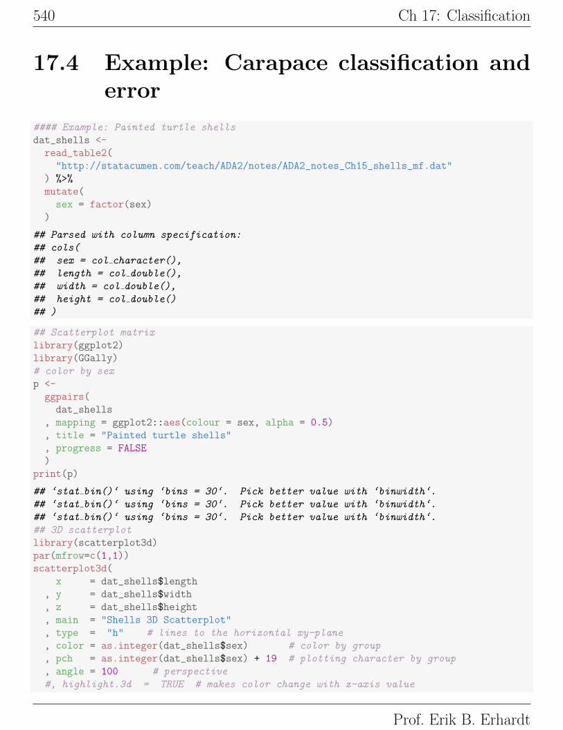
17.4 Example: Carapace classification anderror

#### Example: Painted turtle shells

dat_shells <-

read_table2(

"http://statacumen.com/teach/ADA2/notes/ADA2_notes_Ch15_shells_mf.dat"

) %>%

mutate(

sex = factor(sex)

)

## Parsed with column specification:

## cols(

## sex = col character(),

## length = col double(),

## width = col double(),

## height = col double()

## )

## Scatterplot matrix

library(ggplot2)

library(GGally)

# color by sex

p <-

ggpairs(

dat_shells

, mapping = ggplot2::aes(colour = sex, alpha = 0.5)

, title = "Painted turtle shells"

, progress = FALSE

)

print(p)

## ‘stat bin()‘ using ‘bins = 30‘. Pick better value with ‘binwidth‘.



## 3D scatterplot

library(scatterplot3d)

par(mfrow=c(1,1))

scatterplot3d(

x = dat_shells$length

, y = dat_shells$width

, z = dat_shells$height

, main = "Shells 3D Scatterplot"

, type = "h" # lines to the horizontal xy-plane

, color = as.integer(dat_shells$sex) # color by group

, pch = as.integer(dat_shells$sex) + 19 # plotting character by group

, angle = 100 # perspective

#, highlight.3d = TRUE # makes color change with z-axis value


17.4: Example: Carapace classification and error 541

)

#### Try this!

#### For a rotatable 3D plot, use plot3d() from the rgl library

# ## This uses the R version of the OpenGL (Open Graphics Library)

# #library(rgl)

# rgl::plot3d(

# x = dat_shells£length

# , y = dat_shells£width

# , z = dat_shells£height

# , col = dat_shells£sex %>% as.integer()

# )

Cor : 0.978

F: 0.973

M: 0.95

Cor : 0.963

F: 0.971

M: 0.947

Cor : 0.96

F: 0.966

M: 0.912

sex length width height

sexlength

width

height

0 1 2 3 4 50 1 2 3 4 5 100 120 140 160 180 80 90 100110120130 40 50 60

0

5

10

15

20

25

100

120

140

160

180

80

100

120

40

50

60

Painted turtle shells

Shells 3D Scatterplot

80 100 120 140 160 180

3540

4550

5560

6570

70

80

90

100

110

120

130

140

dat_shells$length

dat_

shel

ls$w

idth

dat_

shel

ls$h

eigh

t

●

●●

●●

●

●

●●

●

●

●

●●

●

●● ●

● ●●

●

●

●●

●

●

●●●

●●●

●

●

●●

●●● ●●●

●●

●●●

As suggested in the partimat() plot below (and by an earlier analysis), classi-

fication based on the length and height of the carapace appears best (considering

only pairs). For this example, we’ll only consider those two features.# classification of observations based on classification methods

# (e.g. lda, qda) for every combination of two variables.

library(klaR)

partimat(

sex ~ length + width + height

, data = dat_shells

, plot.matrix = TRUE

)



FFFF

FFF

FFFFFFF

FFFF

FFFF

F

F

MMM

MMMMMM

MMMMMMMMMMM

MMM

M●

●

Error: 0.188

8090

100

110

120

130

FFFF

F

F F

F FFFFFF FFFF FFF F F

F

M MMMMMMMM

MMM MMMMM MMMMMM

M●

●

Error: 0.188

80 90 100 110 120 130

F F

FFF

F

F

FFF

FFFFF

FFF

F

FFFF

F

MMM

MMMMMM

MMM

MMMMM

MM

MMMMM

●

●

Error: 0.083

3540

4550

5560

65

100 120 140 160

FF FF

F

FF

FFFFF FF FFF

F FF FFF

F

MMMMMMMMMMMM

MMMMM MMMMMMM ●

●

Error: 0.083

35 40 45 50 55 60 65

100

120

140

160

F F

FFF

F

F

F FF

FFFF

F

FFF

F

FF F

F

F

MMM

MMMMMM

MMM

MMMMM

MM

MMMMM

●

●

Error: 0.146

80 90 100 110 120 130

FF FF F

FF

FFFFFFF

FFFF

FF FF

F

F

MMM

MMMMMM

MMMMMM

MM

MM MMMM

M●

●

Error: 0.146

8090

100

110

120

130

100

120

140

160

180

100 120 140 160 180

length

width

35 40 45 50 55 60 65

3540

4550

5560

65

height

The default linear discriminant analysis assumes equal prior probabilities

for males and females.library(MASS)

lda_shells <-

lda(

sex ~ length + height

, data = dat_shells

)

lda_shells

## Call:

## lda(sex ~ length + height, data = dat_shells)

##

## Prior probabilities of groups:

## F M

## 0.5 0.5

##

## Group means:

## length height

## F 136.0417 52.04167

## M 113.4167 40.70833

##

## Coefficients of linear discriminants:

## LD1

## length 0.1370519

## height -0.4890769

The linear discrimant function is in the direction that best separates the



sexes,

LD1 = 0.1371 length +−0.4891 height.

The plot of the lda object shows the groups across the linear discriminant

function. From the klaR package we can get color-coded classification areas

based on a perpendicular line across the LD function.plot(

lda_shells

, dimen = 1

, type = "both"

, col = as.numeric(dat_shells$sex)

)

−4 −3 −2 −1 0 1 2

0.0

0.4

0.8

group F

−4 −3 −2 −1 0 1 2

0.0

0.4

0.8

group M

The constructed table gives the jackknife-based classification and posterior

probabilities of being male or female for each observation in the data set. The

misclassification rate follows.# CV = TRUE does jackknife (leave-one-out) crossvalidation

lda_shells_cv <-

lda(

sex ~ length + height

, data = dat_shells

, CV = TRUE

)

# Create a table of classification and posterior probabilities for each observation



classify_shells <-

data.frame(

sex = dat_shells$sex

, class = lda_shells_cv$class

, error = ""

, post = round(lda_shells_cv$posterior,3)

)

colnames(classify_shells) <-

c(

"sex"

, "class"

, "error"

, paste("post", colnames(lda_shells_cv$posterior), sep="_")

) # "postF" and "postM" column names

# error column

classify_shells$error <-

as.character(classify_shells$error)

classify_agree <-

as.character(as.numeric(dat_shells$sex) - as.numeric(lda_shells_cv$class))

classify_shells$error[!(classify_agree == 0)] <-

classify_agree[!(classify_agree == 0)]

The classification summary table is constructed from the canonical

discriminant functions by comparing the predicted group membership for each

observation to its actual group label. To be precise, if you assume that the sex

for the 24 males are unknown then you would classify each of them correctly.

Similarly, 20 of the 24 females are classified correctly, with the other four classi-

fied as males. The Total Error of 0.0833 is the estimated miscassification rate,

computed as the sum of Rates×Prior over sexes: 0.0833 = 0.1667×0.5+0×0.5.

Are the misclassification results sensible, given the data plots that you saw ear-

lier?

The listing of the posterior probabilities for each sex, by case, gives you

an idea of the clarity of classification, with larger differences between the

male and female posteriors corresponding to more definitive (but not necessarily

correct!) classifications.# print table

classify_shells

## sex class error post_F post_M



## 1 F M -1 0.166 0.834

## 2 F M -1 0.031 0.969

## 3 F F 0.847 0.153

## 4 F F 0.748 0.252

## 5 F F 0.900 0.100

## 6 F F 0.992 0.008

## 7 F F 0.517 0.483

## 8 F F 0.937 0.063

## 9 F F 0.937 0.063

## 10 F F 0.937 0.063

## 11 F M -1 0.184 0.816

## 12 F M -1 0.294 0.706

## 13 F F 0.733 0.267

## 14 F F 0.733 0.267

## 15 F F 0.917 0.083

## 16 F F 0.994 0.006

## 17 F F 0.886 0.114

## 18 F F 0.864 0.136

## 19 F F 1.000 0.000

## 20 F F 0.998 0.002

## 21 F F 1.000 0.000

## 22 F F 1.000 0.000

## 23 F F 0.993 0.007

## 24 F F 0.999 0.001

## 25 M M 0.481 0.519

## 26 M M 0.040 0.960

## 27 M M 0.020 0.980

## 28 M M 0.346 0.654

## 29 M M 0.092 0.908

## 30 M M 0.021 0.979

## 31 M M 0.146 0.854

## 32 M M 0.078 0.922

## 33 M M 0.018 0.982

## 34 M M 0.036 0.964

## 35 M M 0.026 0.974

## 36 M M 0.019 0.981

## 37 M M 0.256 0.744

## 38 M M 0.023 0.977

## 39 M M 0.023 0.977

## 40 M M 0.012 0.988

## 41 M M 0.002 0.998

## 42 M M 0.175 0.825

## 43 M M 0.020 0.980

## 44 M M 0.157 0.843

## 45 M M 0.090 0.910

## 46 M M 0.067 0.933

## 47 M M 0.081 0.919

## 48 M M 0.074 0.926



# Assess the accuracy of the prediction

pred_freq <-

table(

lda_shells_cv$class

, dat_shells$sex

) # row = true sex, col = classified sex

pred_freq

##

## F M

## F 20 0

## M 4 24

prop.table(pred_freq, 2) # proportions by column

##

## F M

## F 0.8333333 0.0000000

## M 0.1666667 1.0000000

# proportion correct for each category

diag(prop.table(pred_freq, 2))

## F M

## 0.8333333 1.0000000

# total proportion correct

sum(diag(prop.table(pred_freq)))

## [1] 0.9166667

# total error rate

1 - sum(diag(prop.table(pred_freq)))

## [1] 0.08333333

A more comprehensive list of classification statistics is given below.library(caret)

confusionMatrix(

data = lda_shells_cv$class # predictions

, reference = dat_shells$sex # true labels

, mode = "sens_spec" # restrict output to relevant summaries

)

## Confusion Matrix and Statistics

##

## Reference

## Prediction F M

## F 20 0

## M 4 24

##

## Accuracy : 0.9167

## 95% CI : (0.8002, 0.9768)

## No Information Rate : 0.5

## P-Value [Acc > NIR] : 7.569e-10



##

## Kappa : 0.8333

##

## Mcnemar's Test P-Value : 0.1336

##

## Sensitivity : 0.8333

## Specificity : 1.0000

## Pos Pred Value : 1.0000

## Neg Pred Value : 0.8571

## Prevalence : 0.5000

## Detection Rate : 0.4167

## Detection Prevalence : 0.4167

## Balanced Accuracy : 0.9167

##

## 'Positive' Class : F

##



17.5 Example: Fisher’s Iris Data cross-validation

I will illustrate cross-validation on Fisher’s iris data first using a test data set,

and then using the jackknife method. The 150 observations were randomly

rearranged and separated into two batches of 75. The 75 observations in the

calibration set were used to develop a classification rule. This rule was applied

to the remaining 75 flowers, which form the test data set. There is no general

rule about the relative sizes of the test data and the training data. Many

researchers use a 50-50 split. Regardless of the split, you should combine the

two data sets at the end of the cross-validation to create the actual rule for

classifying future data.

Below, the half of the indices of the iris data set are randomly selected,

and assigned a label “test”, whereas the rest are “train”. A plot indicates the

two subsamples are similar.#### Example: Fisher's iris data

# The "iris" dataset is included with R in the library(datasets)

data(iris)

str(iris)

## 'data.frame': 150 obs. of 5 variables:

## $ Sepal.Length: num 5.1 4.9 4.7 4.6 5 5.4 4.6 5 4.4 4.9 ...

## $ Sepal.Width : num 3.5 3 3.2 3.1 3.6 3.9 3.4 3.4 2.9 3.1 ...

## $ Petal.Length: num 1.4 1.4 1.3 1.5 1.4 1.7 1.4 1.5 1.4 1.5 ...

## $ Petal.Width : num 0.2 0.2 0.2 0.2 0.2 0.4 0.3 0.2 0.2 0.1 ...

## $ Species : Factor w/ 3 levels "setosa","versicolor",..: 1 1 1 1 1 1 1 1 1 1 ...

# Randomly assign equal train/test by Species strata

# wrote a general function to apply labels given a set of names and proportions

f_assign_groups <-

function(

dat_grp = NULL

, trt_var_name = "test"

, trt_labels = c("train", "test")

, trt_proportions = rep(0.5, 2)

) {## dat_grp <- iris %>% filter(Species == "setosa")

# number of rows of data subset for this group

n_total <- nrow(dat_grp)

# assure that trt_proportions sums to 1

trt_proportions <- trt_proportions / sum(trt_proportions)


17.5: Example: Fisher’s Iris Data cross-validation 549

if (!all.equal(sum(trt_proportions), 1)) {stop("f_assign_groups: trt_proportions can not be coerced to sum to 1.")

}

n_grp <- (n_total * trt_proportions) %>% round()

if (!(sum(n_grp) == n_total)) {# adjust max sample to correct total sample size, is group 1 if equal

ind_max <- which.max(n_grp)

n_diff <- sum(n_grp) - n_total

n_grp[ind_max] <- n_grp[ind_max] - n_diff

}

dat_grp[[trt_var_name]] <-

rep(trt_labels, n_grp) %>%

sample()

return(dat_grp)

}

iris <-

iris %>%

group_by(Species) %>%

group_map(

~ f_assign_groups(

dat_grp = .

, trt_var_name = "test"

, trt_labels = c("train", "test")

, trt_proportions = rep(0.5, 2)

)

, keep = TRUE

) %>%

bind_rows() %>%

ungroup() %>%

mutate(

test = factor(test)

)

summary(iris$test)

## test train

## 75 75

table(iris$Species, iris$test)

##

## test train

## setosa 25 25

## versicolor 25 25

## virginica 25 25




library(ggplot2)

library(GGally)

p <- ggpairs(subset(iris, test == "train")[,c(5,1,2,3,4)]

, mapping = ggplot2::aes(colour = Species, alpha = 0.5)

, title = "train"

, progress=FALSE

)

print(p)





p <- ggpairs(subset(iris, test == "test")[,c(5,1,2,3,4)]

, mapping = ggplot2::aes(colour = Species, alpha = 0.5)

, title = "test"

, progress=FALSE

)

print(p)





Cor : −0.18

setosa: 0.794

versicolor: 0.476

virginica: 0.342

Cor : 0.892

setosa: 0.516

versicolor: 0.732

virginica: 0.824

Cor : −0.454

setosa: 0.325

versicolor: 0.575

virginica: 0.368

Cor : 0.853

setosa: 0.528

versicolor: 0.554

virginica: 0.252

Cor : −0.388

setosa: 0.449

versicolor: 0.671

virginica: 0.484

Cor : 0.964

setosa: 0.385

versicolor: 0.785

virginica: 0.322

Species Sepal.Length Sepal.Width Petal.Length Petal.Width

Species

Sepal.Length

Sepal.W

idthP

etal.LengthP

etal.Width

0 5 10 0 5 10 0 5 10 5 6 7 2.0 2.5 3.0 3.5 4.0 4.5 2 4 6 0.0 0.5 1.0 1.5 2.0 2.5

0

5

10

15

20

25

5

6

7

2.0

2.5

3.0

3.5

4.0

4.5

2

4

6

0.0

0.5

1.0

1.5

2.0

2.5

train

Cor : −0.0503

setosa: 0.733

versicolor: 0.588

virginica: 0.551

Cor : 0.855

setosa: −0.0397

versicolor: 0.809

virginica: 0.901

Cor : −0.402

setosa: −0.0166

versicolor: 0.553

virginica: 0.43

Cor : 0.789

setosa: 0.0788

versicolor: 0.599

virginica: 0.309

Cor : −0.343

setosa: 0.0409

versicolor: 0.665

virginica: 0.593

Cor : 0.962

setosa: 0.291

versicolor: 0.792

virginica: 0.326

Species Sepal.Length Sepal.Width Petal.Length Petal.Width

Species

Sepal.Length

Sepal.W

idthP

etal.LengthP

etal.Width

0 5 10 150 5 10 150 5 10 15 5 6 7 8 2.5 3.0 3.5 4.0 1 2 3 4 5 6 0.0 0.5 1.0 1.5 2.0 2.5

0

5

10

15

20

25

5

6

7

8

2.5

3.0

3.5

4.0

2

4

6

0.0

0.5

1.0

1.5

2.0

2.5

test

As suggested in the partimat() plot below, we should expect Sepal.Length

to potentially not contribute much to the classification, since (pairwise) more

errors are introduced with that variable than between other pairs. (In fact,

we’ll see below that the coefficients for Sepal.Length is smallest.)# classification of observations based on classification methods


library(klaR)

partimat(



Species ~ Sepal.Length + Sepal.Width + Petal.Length + Petal.Width

, data = subset(iris, test == "train")

, plot.matrix = TRUE

)

sss

s

s

s s

s

s

s

s

s sss s

s

s

ss

s

ss

s s v v

vv

v

v

v vvv

v

v

v

v

vv

v

v v

v

v

v

v

vv

v

v vv

v

v

vv

v

v

v

v

vvv

v vv vvv

v

v

v

v

●

●●

Error: 0.173

2.0

2.5

3.0

3.5

4.0

sss

ss

sss s

s

ss

s

s

s

ss

s ss

s

ss

ss

v

vv

v

v

v

vv

vvv

v

vv

vv

vvv

v

vv

v

v

v

vv

v

vv

v v

v

vv

v

v

v

v

v v

vvvvv

vv

vv

●

●

●

Error: 0.173

2.0 2.5 3.0 3.5 4.0

sss ss

s ssss

ssss

ss sssss

sss s

vv

vv v

vv

v

v

vv

vv

v vv

v v

vv vv

v

vv

vv

v

v vvv

v

vv

vv

v

v

vv vv

v

vvv vv

v

●

●

●

Error: 0.027

12

34

56

ssss

s

ssss

s

ss

s

s

s

ss

sss

s

ss

ss

v

vv

v

v

v

vv

v vv

v

vvvv

vv

v

v

vv

v

v

v

vv

v

vv

vv

v

vv

v

v

v

v

v v

vv

v vvvvv

v

●

●

●

Error: 0.027

1 2 3 4 5 6

s ss ss

sss ss

ssss

ss ss sss

ssss

vv

vv v

vv

v

v

vv

vv

vvv

v v

vvv v

v

vv

vvv

v vv v

v

vv

vv

v

v

vvvvv

vvv v vv

●

●

●

Error: 0.027

sss

s

s

ss

s

s

s

s

s sss s

s

s

ss

s

ss

ss v v

vv

v

v

v vv v

v

v

v

v

vv

v

v v

v

v

v

v

vv

v

v vv

v

v

vv

v

v

v

v

vvv

vvvv vv

v

v

v

v

●

●●

Error: 0.027

sss sss ssss

ss sss s sssss sss s

v vvv

v

v

v vvv

v

v

v

v

v

v

vv

vvvv

v

vv

v

v vvvv

v

v

vv

v

v

v v

v

v

v

v vvv

v v

v

v

●

●

●

Error: 0.04

0.5

1.0

1.5

2.0

2.5

4.5 5.5 6.5 7.5

ssss

s

ssss

s

ss

s

s

s

ss

ss s

s

ss

ss

v

vv

v

v

v

vv

v vv

v

vv

v v

vv

v

v

vv

v

v

v

vv

v

vv

v v

v

vv

v

v

v

v

v v

vv

vvvvv

vv

●

●

●

Error: 0.04

0.5 1.0 1.5 2.0 2.5

4.5

5.5

6.5

7.5

s ss sssss ss

ssssss ss sss s

sss

vvvv

v

v

vvvv

v

v

v

v

v

v

vv

v vv v

v

vv

v

vvvvv

v

v

vv

v

v

vv

v

v

v

vvvv

v v

v

v

●

●

●

Error: 0.04

2.0 2.5 3.0 3.5 4.0

sss

s

s

ss

s

s

s

s

sssss

s

s

s s

s

ss

ss vv

vv

v

v

vvv v

v

v

v

v

v v

v

v v

v

v

v

v

vv

v

vvv

v

v

vv

v

v

v

v

vvv

v v vvvv

v

v

v

v

●

●●

Error: 0.04

2.0

2.5

3.0

3.5

4.0

ssssssssss

ss sss ssssss s

sss

v vvv

v

v

v vvv

v

v

v

v

v

v

vv

vvvv

v

vv

v

v vvvv

v

v

vv

v

v

v v

v

v

v

vv vv

vv

v

v

●

●

●

Error: 0.04

1 2 3 4 5 6

sssss

sssss

ssss

sssss ss

ssss

vvvv v

vv

v

v

vv

vv

vv v

v v

vvvv

v

vv

vvv

v vv v

v

vv

vv

v

v

vv v v

v

vvvv v

v

●

●

●

Error: 0.04

12

34

56

4.5

5.5

6.5

7.5

4.5 5.5 6.5 7.5

Sepal.Length

Sepal.Width

Petal.Length

0.5 1.0 1.5 2.0 2.5

0.5

1.0

1.5

2.0

2.5

Petal.Width

library(MASS)

lda_iris <-

lda(



)

lda_iris

## Call:

## lda(Species ~ Sepal.Length + Sepal.Width + Petal.Length + Petal.Width,

## data = subset(iris, test == "train"))

##


## setosa versicolor virginica

## 0.3333333 0.3333333 0.3333333

##



## Group means:

## Sepal.Length Sepal.Width Petal.Length Petal.Width

## setosa 4.980 3.476 1.444 0.240

## versicolor 5.904 2.776 4.324 1.352

## virginica 6.572 2.964 5.524 2.032

##


## LD1 LD2

## Sepal.Length 0.7559841 -0.983584

## Sepal.Width 1.5248395 -1.244256

## Petal.Length -2.1694100 1.696405

## Petal.Width -2.7048160 -3.526479

##

## Proportion of trace:

## LD1 LD2

## 0.9911 0.0089

The linear discrimant functions that best classify the Species in the training

set are

LD1 = 0.756 sepalL + 1.525 sepalW +−2.169 petalL +−2.705 petalW

LD2 = −0.9836 sepalL +−1.244 sepalW + 1.696 petalL +−3.526 petalW.

The plots of the lda object shows the data on the LD scale.plot(lda_iris, dimen = 1, col = as.numeric(iris$Species))

plot(lda_iris, dimen = 2, col = as.numeric(iris$Species), abbrev = 3)

#pairs(lda_iris, col = as.numeric(iris£Species))

−10 −5 0 5 10

0.0

0.3

0.6

group setosa

−10 −5 0 5 10

0.0

0.3

0.6

group versicolor

−10 −5 0 5 10

0.0

0.3

0.6

group virginica

−5 0 5

−5

05

LD1

LD2 stssts

sts

sts

sts

stssts

stssts

sts

stssts

stssts stssts

sts

stssts

sts

sts

sts sts

stssts

vrsvrsvrs

vrs

vrs

vrs

vrs

vrs

vrs

vrs

vrs

vrsvrs

vrs

vrs

vrs

vrs

vrsvrs

vrsvrs

vrs

vrs

vrsvrs

vrg

vrgvrg

vrg

vrg

vrg

vrg

vrg

vrg

vrg

vrg

vrg

vrg

vrg

vrg

vrg

vrgvrg

vrg

vrg

vrg

vrg

vrg

vrg

vrg



# CV = TRUE does jackknife (leave-one-out) crossvalidation

lda_iris_cv <-

lda(



, CV = TRUE

)


classify_iris <-

data.frame(

Species = iris %>% filter(test == "train") %>% pull(Species)

, class = lda_iris_cv$class

, error = ""

, round(lda_iris_cv$posterior, 3)

)

colnames(classify_iris) <-

c("Species", "class", "error"

, paste("post", colnames(lda_iris_cv$posterior), sep="_")

)

# error column, a non-zero is a classification error

classify_iris <-

classify_iris %>%

mutate(

error = as.numeric(Species) - as.numeric(class)

)

The misclassification error is very low within the training set.library(caret)

confusionMatrix(

data = classify_iris$class # predictions

, reference = classify_iris$Species # true labels


)


##

## Reference

## Prediction setosa versicolor virginica

## setosa 25 0 0

## versicolor 0 23 2

## virginica 0 2 23

##

## Overall Statistics

##


## 95% CI : (0.869, 0.9853)




## P-Value [Acc > NIR] : < 2.2e-16

##

## Kappa : 0.92

##

## Mcnemar's Test P-Value : NA

##

## Statistics by Class:

##

## Class: setosa Class: versicolor Class: virginica

## Sensitivity 1.0000 0.9200 0.9200

## Specificity 1.0000 0.9600 0.9600

## Pos Pred Value 1.0000 0.9200 0.9200

## Neg Pred Value 1.0000 0.9600 0.9600

## Prevalence 0.3333 0.3333 0.3333

## Detection Rate 0.3333 0.3067 0.3067

## Detection Prevalence 0.3333 0.3333 0.3333

## Balanced Accuracy 1.0000 0.9400 0.9400

How well does the LD functions constructed on the training data predict

the Species in the independent test data?# predict the test data from the training data LDFs

pred_iris <-

predict(

lda_iris

, newdata = iris %>% filter(test == "test")

)


classify_iris <-

data.frame(

Species = iris %>% filter(test == "test") %>% pull(Species)

, class = pred_iris$class

, error = ""

, round(pred_iris$posterior, 3)

)

colnames(classify_iris) <-

c("Species", "class", "error"

, paste("P", colnames(lda_iris_cv$posterior), sep="_")

)


classify_iris <-

classify_iris %>%

mutate(

error = as.numeric(Species) - as.numeric(class)

)



# print table

classify_iris

## Species class error P_setosa P_versicolor P_virginica

## 1 setosa setosa 0 1 0.000 0.000

## 2 setosa setosa 0 1 0.000 0.000

## 3 setosa setosa 0 1 0.000 0.000

## 4 setosa setosa 0 1 0.000 0.000

## 5 setosa setosa 0 1 0.000 0.000

## 6 setosa setosa 0 1 0.000 0.000

## 7 setosa setosa 0 1 0.000 0.000

## 8 setosa setosa 0 1 0.000 0.000

## 9 setosa setosa 0 1 0.000 0.000

## 10 setosa setosa 0 1 0.000 0.000

## 11 setosa setosa 0 1 0.000 0.000

## 12 setosa setosa 0 1 0.000 0.000

## 13 setosa setosa 0 1 0.000 0.000

## 14 setosa setosa 0 1 0.000 0.000

## 15 setosa setosa 0 1 0.000 0.000

## 16 setosa setosa 0 1 0.000 0.000

## 17 setosa setosa 0 1 0.000 0.000

## 18 setosa setosa 0 1 0.000 0.000

## 19 setosa setosa 0 1 0.000 0.000

## 20 setosa setosa 0 1 0.000 0.000

## 21 setosa setosa 0 1 0.000 0.000

## 22 setosa setosa 0 1 0.000 0.000

## 23 setosa setosa 0 1 0.000 0.000

## 24 setosa setosa 0 1 0.000 0.000

## 25 setosa setosa 0 1 0.000 0.000

## 26 versicolor versicolor 0 0 1.000 0.000



























## 51 virginica virginica 0 0 0.005 0.995

























library(caret)

confusionMatrix(

data = classify_iris$class # predictions

, reference = classify_iris$Species # true labels


)


##

## Reference

## Prediction setosa versicolor virginica

## setosa 25 0 0

## versicolor 0 25 0

## virginica 0 0 25

##


##

## Accuracy : 1

## 95% CI : (0.952, 1)




## P-Value [Acc > NIR] : < 2.2e-16

##

## Kappa : 1

##


##


##

## Class: setosa Class: versicolor Class: virginica

## Sensitivity 1.0000 1.0000 1.0000

## Specificity 1.0000 1.0000 1.0000

## Pos Pred Value 1.0000 1.0000 1.0000

## Neg Pred Value 1.0000 1.0000 1.0000

## Prevalence 0.3333 0.3333 0.3333

## Detection Rate 0.3333 0.3333 0.3333



The classification rule based on the training set works extremely well with

the test data. Do not expect such nice results on all classification problems!

Usually the error rate is slightly higher on the test data than on the training

data.

It is important to recognize that statistically significant differences (MANOVA)

among groups on linear discriminant function scores do not necessarily translate

into accurate classification rules! This is because there may still be substantial

overlap in the populations, which will increase classification error rates.



17.5.1 Stepwise variable selection for classification

Stepwise variable selection for classification can be performed using package

klaR function stepclass() using any specified classification function. Classifi-

cation performance is estimated by selected from one of Uschi’s classification

performance measures.

The resulting model can be very sensitive to the starting model. Below, the

first model starts full and ends full. The second model starts empty and ends

after one variable is added. Note that running this repeatedly could result in

slightly different models because the k-fold crossvalidation partitions the data

at random. The formula object gives the selected model.# reset the data

data(iris)

library(klaR)

# start with full model and do stepwise (direction = "backward")

step_iris_b <-

stepclass(


, data = iris

, method = "lda"

, improvement = 0.01 # stop criterion: improvement less than 1%

# default of 5% is too coarse

, direction = "backward"

)

## ‘stepwise classification’, using 10-fold cross-validated correctness rate of method

lda’.

## 150 observations of 4 variables in 3 classes; direction: backward

## stop criterion: improvement less than 1%.

## correctness rate: 0.98; starting variables (4): Sepal.Length, Sepal.Width, Petal.Length, Petal.Width

##

## hr.elapsed min.elapsed sec.elapsed

## 0.00 0.00 0.23

plot(step_iris_b, main = "Start = full model, backward selection")

step_iris_b$formula

## Species ~ Sepal.Length + Sepal.Width + Petal.Length + Petal.Width

## <environment: 0x000001cf29f80350>

# start with empty model and do stepwise (direction = "both")

step_iris_f <-

stepclass(


, data = iris



, method = "lda"

, improvement = 0.01 # stop criterion: improvement less than 1%

, direction = "forward"

)

## ‘stepwise classification’, using 10-fold cross-validated correctness rate of method

lda’.

## 150 observations of 4 variables in 3 classes; direction: forward

## stop criterion: improvement less than 1%.

## correctness rate: 0.96; in: "Petal.Width"; variables (1): Petal.Width

##

## hr.elapsed min.elapsed sec.elapsed

## 0.00 0.00 0.25

plot(step_iris_f, main = "Start = empty model, forward selection")

step_iris_f$formula

## Species ~ Petal.Width

## <environment: 0x000001cf25ca4270>

●

0.6

0.8

1.0

1.2

1.4

Start = full model, backward selection

estim

ated

cor

rect

ness

rat

e

STA

RT

●

●

0.0

0.2

0.4

0.6

0.8

Start = empty model, forward selection

estim

ated

cor

rect

ness

rat

e

STA

RT

+ P

etal

.Wid

th

Given your selected model, you can then go on to fit your classification

model by using the formula from the stepclass() object.library(MASS)

lda_iris_step <-

lda(

step_iris_b$formula

, data = iris

)

lda_iris_step

## Call:



## lda(step_iris_b$formula, data = iris)

##


## setosa versicolor virginica

## 0.3333333 0.3333333 0.3333333

##

## Group means:

## Sepal.Length Sepal.Width Petal.Length Petal.Width

## setosa 5.006 3.428 1.462 0.246

## versicolor 5.936 2.770 4.260 1.326

## virginica 6.588 2.974 5.552 2.026

##


## LD1 LD2

## Sepal.Length 0.8293776 0.02410215

## Sepal.Width 1.5344731 2.16452123

## Petal.Length -2.2012117 -0.93192121

## Petal.Width -2.8104603 2.83918785

##


## LD1 LD2

## 0.9912 0.0088

Note that if you have many variables, you may wish to use the alternate

syntax below to specify your formula (see the help ?stepclass for this example).iris_d <- iris[, 1:4] # the data

iris_c <- iris[, 5] # the classes

sc_obj <- stepclass(iris_d, iris_c, "lda", start.vars = "Sepal.Width")

sc_obj


17.6: Example: Analysis of Admissions Data 561

17.6 Example: Analysis of Admissions Data

The admissions officer of a business school has used an index of undergraduate

GPA and management aptitude test scores (GMAT) to help decide which ap-

plicants should be admitted to graduate school. The data below gives the GPA

and GMAT scores for recent applicants who are classified as admit (A), border-

line (B), or not admit (N). An equal number of A, B, and N’s (roughly) were

selected from their corresponding populations (Johnson and Wichern, 1988).#### Example: Business school admissions data

dat_business <-

read_table2(

"http://statacumen.com/teach/ADA2/notes/ADA2_notes_Ch17_business.dat"

) %>%

mutate(

admit = admit %>% factor()

)

## Parsed with column specification:

## cols(

## admit = col character(),

## gpa = col double(),

## gmat = col double()

## )


library(ggplot2)

library(GGally)

p <-

ggpairs(

dat_business

, mapping = ggplot2::aes(colour = admit, alpha = 0.5)

, progress = FALSE

)

print(p)



library(ggplot2)

p <- ggplot(dat_business, aes(x = gpa, y = gmat, colour = admit, label = admit))

p <- p + geom_text(size = 6)

p <- p + theme(legend.position="none") # remove legend with fill colours

print(p)



Cor : 0.442

A: 0.147

B: −0.331

N: 0.507

admit gpa gmat

admit

gpagm

at0 2 4 60 2 4 60 2 4 6 2.0 2.5 3.0 3.5 300 400 500 600 700

0

10

20

30

2.0

2.5

3.0

3.5

300

400

500

600

700

A

A A

AA

A

A

A

A

AA A

AA

A

AA

AA

AA

AA

A

A

A

A

A

A

A

A

A

N

N

N

N

N

N

N N

N N

N

N

N

NN

NN

N

N

N

N

N

NN

N

N

B

B

B

B

B

B

B

B

B

BB

BBB

B

B

B BB

B

B

B

B

BB

B

B

B

B

B

B

300

400

500

600

700

2.0 2.5 3.0 3.5gpa

gmat

The officer wishes to use these data to develop a more quantitative (i.e., less

subjective) approach to classify prospective students. Historically, about 20%

of all applicants have been admitted initially, 10% are classified as borderline,

and the remaining 70% are not admitted. The officer would like to keep these

percentages roughly the same in the future.

This is a natural place to use discriminant analysis. Let us do a more

careful analysis here, paying attention to underlying assumptions of normality

and equal covariance matrices.

The GPA and GMAT distributions are reasonably symmetric. Although

a few outliers are present, it does not appear that any transformation will

eliminate the outliers and preserve the symmetry. Given that the outliers are

not very extreme, I would analyze the data on this scale. Except for the outliers,

the spreads (IQRs) are roughly equal across groups within GPA and GMAT. I

will look carefully at the variance-covariance matrices later.

There is a fair amount of overlap between the borderline and other groups,

but this should not be too surprising. Otherwise these applicants would not be

borderline!



17.6.1 Further Analysis of the Admissions Data

The assumption of constant variance-covariance matrices is suspect. The GPA

and GMAT variances are roughly constant across groups, but the correlation

between GPA and GMAT varies greatly over groups.# Covariance matrices by admit

by(dat_business[, 2:3], dat_business$admit, cov)

## dat_business$admit: A

## gpa gmat

## gpa 0.05866734 2.857601

## gmat 2.85760081 6479.990927

## ----------------------------------------------------

## dat_business$admit: B

## gpa gmat

## gpa 0.05422559 -4.87757

## gmat -4.87756989 4002.76129

## ----------------------------------------------------

## dat_business$admit: N

## gpa gmat

## gpa 0.05602785 10.01171

## gmat 10.01170769 6973.16462

# Correlation matrices by admit

by(dat_business[, 2:3], dat_business$admit, FUN = stats::cor)

## dat_business$admit: A

## gpa gmat

## gpa 1.0000000 0.1465602

## gmat 0.1465602 1.0000000

## ----------------------------------------------------

## dat_business$admit: B

## gpa gmat

## gpa 1.0000000 -0.3310713

## gmat -0.3310713 1.0000000

## ----------------------------------------------------

## dat_business$admit: N

## gpa gmat

## gpa 1.0000000 0.5065137

## gmat 0.5065137 1.0000000

Assuming equal variance-covariance matrices, both GPA and GMAT are

important for discriminating among entrance groups. This is consistent with

the original data plots.# classification of observations based on classification methods


library(klaR)



partimat(

admit ~ gmat + gpa

, data = dat_business

, plot.matrix = FALSE

)

2.0 2.5 3.0 3.5

300

400

500

600

700

gpa

gmat

A

A A

AA

A

A

A

A

AA A

AA

A

AA

AA

AA

AA

A

A

A

A

A

A

A

A

A

N

N

N

N

N

N

NN

N N

N

N

N

NN

NN

N

N

N

N

N

NN

N

N

B

B

B

B

B

B

B

B

B

B

B

BB

B

B

B

B BB

B

B

B

B

B

B

B

B

B

B

B

B

●

●●

app. error rate: 0.157

Partition Plot

library(MASS)

lda_business <-

lda(

admit ~ gpa + gmat


)

lda_business

## Call:

## lda(admit ~ gpa + gmat, data = dat_business)

##


## A B N

## 0.3595506 0.3483146 0.2921348

##



## Group means:

## gpa gmat

## A 3.321875 554.4062

## B 3.004516 454.1935

## N 2.400385 443.7308

##


## LD1 LD2

## gpa -3.977912929 -1.48346456

## gmat -0.003057846 0.01292319

##


## LD1 LD2

## 0.9473 0.0527

The linear discrimant functions that best classify the admit are

LD1 = −3.978 gpa +−0.003058 gmat

LD2 = −1.483 gpa + 0.01292 gmat,

interpretted as a weighted average of the scores and a contrast of the scores.

The plots of the lda() object shows the data on the LD scale.plot(lda_business, dimen = 1)

plot(lda_business, dimen = 2, col = as.numeric(dat_business$admit))

#pairs(lda_business, col = as.numeric(dat_business£admit))

−4 −2 0 2 4

0.0

0.2

0.4

0.6

group A

−4 −2 0 2 4

0.0

0.2

0.4

0.6

group B

−4 −2 0 2 4

0.0

0.2

0.4

0.6

group N

−2 0 2 4

−2

02

4

LD1

LD2

A

AA

A

A

AA

A

A

A AAA

A

A

A

AA

A AAA

A

A

A

A

AA

A

A

A

A

N

N

N

N

N

N

NN

NN

N N

N

NN

NN

N

N

N

N

N N

N

N

N

B

B

B

B

B

B

B

B

B

B

B

B

BB

B

B

B

BB

B

B

B

B

B

B

B

B

B

B

B

B




lda_business_cv <-

lda(

admit ~ gpa + gmat


, CV = TRUE

)


classify_business <-

data.frame(

admit = dat_business$admit

, class = lda_business_cv$class

, error = ""

, round(lda_business_cv$posterior, 3)

)

colnames(classify_business) <-

c("admit", "class", "error"

, paste("post", colnames(lda_business_cv$posterior), sep="_")

)



classify_business %>%

mutate(

error = as.numeric(admit) - as.numeric(class)

)

The misclassification error within the training set is reasonably low, given

the overlap between the B group and the others, and never a misclassification

between A and N.library(caret)

confusionMatrix(

data = classify_business$class # predictions

, reference = classify_business$admit # true labels


)


##

## Reference

## Prediction A B N

## A 26 3 0

## B 6 25 3

## N 0 3 23

##


##




## 95% CI : (0.7373, 0.9025)


## P-Value [Acc > NIR] : < 2.2e-16

##

## Kappa : 0.7463

##


##


##

## Class: A Class: B Class: N

## Sensitivity 0.8125 0.8065 0.8846

## Specificity 0.9474 0.8448 0.9524

## Pos Pred Value 0.8966 0.7353 0.8846

## Neg Pred Value 0.9000 0.8909 0.9524

## Prevalence 0.3596 0.3483 0.2921

## Detection Rate 0.2921 0.2809 0.2584





17.6.2 Classification Using Unequal Prior Probabil-ities

A new twist to this problem is that we have prior information on the rela-

tive sizes of the populations. Historically 20% of applicants are admitted, 10%

are borderline, and 70% are not admitted. This prior information is incorpo-

rated into the classification rule by using a prior option with lda(). The prior

probabilities are assumed to be equal when this statement is omitted. The

classification rule for unequal prior probabilities uses both the M -distance and

the prior probability for making decisions, as outlined below.

When the prior probabilities are unequal, classification is based on the gen-

eralized distance to group j:

D2j (X) = (X − X̄j)

′S−1(X − X̄j)− 2 log(PRIORj),

or on the estimated posterior probability of membership in group j:

Pr(j|X) =exp{−0.5D2

j (X)}∑k exp{−0.5D2

k(X)}.

Here S is the pooled covariance matrix, and log(PRIORj) is the (natural) log

of the prior probability of being in group j. As before, you classify observa-

tion X into the group that it is closest to in terms of generalized distance, or

equivalently, into the group with the maximum posterior probability.

Note that−2 log(PRIORj) exceeds zero, and is extremely large when PRIORj

is near zero. The generalized distance is the M -distance plus a penalty term

that is large when the prior probability for a given group is small. If the prior

probabilities are equal, the penalty terms are equal so the classification rule

depends only on the M -distance.

The penalty makes it harder (relative to equal probabilities) to classify into

a low probability group, and easier to classify into high probability groups. In

the admissions data, an observation has to be very close to the B or A groups

to not be classified as N.



Note that in the analysis below, we make the tenuous assumption that the

population covariance matrices are equal. We also have 6 new observations

that we wish to classify. These observations are entered as a test data set with

missing class levels.# new observations to classify

dat_business_test <-

read.table(text = "

admit gpa gmat

NA 2.7 630

NA 3.3 450

NA 3.4 540

NA 2.8 420

NA 3.5 340

NA 3.0 500

", header = TRUE)

With priors, the LDs are different.library(MASS)

lda_business <-

lda(

admit ~ gpa + gmat

, prior = c(0.2, 0.1, 0.7)


)

lda_business

## Call:

## lda(admit ~ gpa + gmat, data = dat_business, prior = c(0.2, 0.1,

## 0.7))

##


## A B N

## 0.2 0.1 0.7

##

## Group means:

## gpa gmat

## A 3.321875 554.4062

## B 3.004516 454.1935

## N 2.400385 443.7308

##


## LD1 LD2

## gpa -4.014778092 -1.38058511

## gmat -0.002724201 0.01299761

##


## LD1 LD2

## 0.9808 0.0192



About 1/2 of the borderlines in the calibration set are misclassified. This is

due to the overlap of the B group with the other 2 groups, but also reflects the

low prior probability for the borderline group. The classification rule requires

strong evidence that an observation is borderline before it can be classified as

such.# CV = TRUE does jackknife (leave-one-out) crossvalidation

lda_business_cv <-

lda(

admit ~ gpa + gmat

, prior = c(0.2, 0.1, 0.7)


, CV = TRUE

)



data.frame(


, class = lda_business_cv$class

, error = ""

, round(lda_business_cv$posterior, 3)

)



, paste("post", colnames(lda_business_cv$posterior), sep="_")

)




mutate(


)

# print table, errors only

classify_business[!(classify_business$error == 0), ]

## admit class error post_A post_B post_N

## 29 A B -1 0.027 0.557 0.416

## 30 A N -2 0.114 0.383 0.503

## 31 A B -1 0.045 0.595 0.360

## 35 N A 2 0.442 0.273 0.285

## 36 N B 1 0.033 0.516 0.451

## 59 B N -1 0.001 0.044 0.955

## 60 B N -1 0.002 0.016 0.982

## 61 B N -1 0.126 0.329 0.545

## 66 B A 1 0.747 0.253 0.000



## 67 B N -1 0.161 0.412 0.428

## 68 B N -1 0.037 0.277 0.686

## 71 B N -1 0.059 0.227 0.714

## 72 B N -1 0.017 0.089 0.894

## 74 B N -1 0.070 0.129 0.801

## 75 B N -1 0.020 0.146 0.834

## 82 B N -1 0.107 0.344 0.549

## 85 B A 1 0.758 0.233 0.009

## 86 B A 1 0.979 0.021 0.001

## 87 B A 1 0.627 0.365 0.008

## 88 B A 1 0.633 0.367 0.000

library(caret)

confusionMatrix(




)


##

## Reference

## Prediction A B N

## A 29 5 1

## B 2 16 1

## N 1 10 24

##


##


## 95% CI : (0.6745, 0.857)


## P-Value [Acc > NIR] : 1.414e-15

##

## Kappa : 0.6643

##


##


##


## Sensitivity 0.9062 0.5161 0.9231

## Specificity 0.8947 0.9483 0.8254

## Pos Pred Value 0.8286 0.8421 0.6857

## Neg Pred Value 0.9444 0.7857 0.9630

## Prevalence 0.3596 0.3483 0.2921

## Detection Rate 0.3258 0.1798 0.2697





The test data cases were entered with missing group IDs. The classification

table compares the group IDs, which are unknown, to the ID for the group into

which an observation is classified. These two labels differ, so all the test data

cases are identified as misclassified. Do not be confused by this! Just focus on

the classification for each case, and ignore the other summaries.# predict the test data from the training data LDFs

pred_business <-

predict(

lda_business

, newdata = dat_business_test

)


classify_business_test <-

data.frame(

admit = dat_business_test$admit

, class = pred_business$class

#, error = ""

, round(pred_business$posterior, 3)

)

colnames(classify_business_test) <-

c("admit", "class"#, "error"

, paste("post", colnames(pred_business$posterior), sep="_")

)

# print table

dat_business_test_class <-

dat_business_test %>%

bind_cols(classify_business_test)

dat_business_test_class

## admit gpa gmat admit1 class post_A post_B post_N

## 1 NA 2.7 630 NA N 0.102 0.074 0.824

## 2 NA 3.3 450 NA A 0.629 0.367 0.004

## 3 NA 3.4 540 NA A 0.919 0.081 0.000

## 4 NA 2.8 420 NA N 0.026 0.297 0.676

## 5 NA 3.5 340 NA B 0.461 0.538 0.001

## 6 NA 3.0 500 NA B 0.385 0.467 0.148

Except for observation 5, the posterior probabilities for the test cases give

strong evidence in favor of classification into a specific group.library(ggplot2)



p <- p + geom_text(data = dat_business_test_class



, aes(x = gpa, y = gmat, colour = class, label = class)

, size = 6)


p <- p + labs(caption = "Large letters are predicted admit classes.")

print(p)

A

AA

A

A

A

A

A

A

A

AA

A

A

A

A

A

A

A

AA

AA

A

A

A

A

A

A

A

A

A

N

N

N

N

N

N

NN

N N

N

N

N

NN

N

N

N

N

N

N

N

NN

N

N

B

B

B

B

B

B

B

B

B

B

B

B

BB

B

B

B B

B

B

B

B

B

B

B

B

B

B

B

B

B

N

A

A

N

B

B

300

400

500

600

700

2.0 2.5 3.0 3.5gpa

gmat

Large letters are predicted admit classes.



17.6.3 Classification With Unequal Covariance Ma-trices, QDA

The assumption of multivariate normal populations with equal covariance ma-

trices is often unrealistic. Although there are no widely available procedures

for MANOVA or stepwise variable selection in discriminant analysis that relax

these assumptions, there are a variety of classification rules that weaken one or

both of these assumptions. The qda() function is a quadratic discriminant

classification rule that assumes normality but allows unequal covari-

ance matrices.

The quadratic discriminant classification rule is based on the generalized

distance to group j:

D2j (X) = (X − X̄j)

′S−1j (X − X̄j)− 2 log(PRIORj) + log |Sj|,

or equivalently, the posterior probability of membership in group j:

Pr(j|X) =exp{−0.5D2

j (X)}∑k exp{−0.5D2

k(X)}.

Here Sj is the sample covariance matrix from group j and log |Sj| is the log

of the determinant of this covariance matrix. The determinant penalty term is

large for groups having large variability. The rule is not directly tied to linear

discriminant function variables, so interpretation and insight into this method

is less straightforward.

There is evidence that quadratic discrimination does not improve misclas-

sification rates in many problems with small to modest sample sizes, in part,

because the quadratic rule requires an estimate of the covariance matrix for

each population. A modest to large number of observations is needed to ac-

curately estimate variances and correlations. I often compute the linear and

quadratic rules, but use the linear discriminant analysis unless the quadratic

rule noticeably reduces the misclassification rate.

Recall that the GPA and GMAT sample variances are roughly constant

across admission groups, but the correlation between GPA and GMAT varies

widely across groups.



The quadratic rule does not classify the training data noticeably better

than the linear discriminant analysis. The individuals in the test data have the

same classifications under both approaches. Assuming that the optimistic error

rates for the two rules were “equally optimistic”, I would be satisfied with the

standard linear discriminant analysis, and would summarize my analysis based

on this approach. Additional data is needed to decide whether the quadratic

rule might help reduce the misclassification rates.# classification of observations based on classification methods

# (e.g. qda, qda) for every combination of two variables.

library(klaR)

partimat(

admit ~ gmat + gpa



, method = "lda"

, main = "LDA partition"

)

partimat(

admit ~ gmat + gpa



, method = "qda"

, main = "QDA partition"

)

2.0 2.5 3.0 3.5

300

400

500

600

700

gpa

gmat

A

A A

AA

A

A

A

A

AA A

AA

A

AA

AA

AA

AA

A

A

A

A

A

A

A

A

A

N

N

N

N

N

N

NN

N N

N

N

N

NN

NN

N

N

N

N

N

NN

N

N

B

B

B

B

B

B

B

B

B

B

B

BB

B

B

B

B BB

B

B

B

B

B

B

B

B

B

B

B

B

●

●●


LDA partition

2.0 2.5 3.0 3.5

300

400

500

600

700

gpa

gmat

A

A A

AA

A

A

A

A

AA A

AA

A

AA

AA

AA

AA

A

A

A

A

A

A

A

A

A

N

N

N

N

N

N

NN

N N

N

N

N

NN

NN

N

N

N

N

N

NN

N

N

B

B

B

B

B

B

B

B

B

B

B

BB

B

B

B

B BB

B

B

B

B

B

B

B

B

B

B

B

B

●

●●


QDA partition



library(MASS)

qda_business <-

qda(

admit ~ gpa + gmat

, prior = c(0.2, 0.1, 0.7)


)

qda_business

## Call:

## qda(admit ~ gpa + gmat, data = dat_business, prior = c(0.2, 0.1,

## 0.7))

##


## A B N

## 0.2 0.1 0.7

##

## Group means:

## gpa gmat

## A 3.321875 554.4062

## B 3.004516 454.1935

## N 2.400385 443.7308


qda_business_cv <-

qda(

admit ~ gpa + gmat

, prior = c(0.2, 0.1, 0.7)


, CV = TRUE

)



data.frame(


, class = qda_business_cv$class

, error = ""

, round(qda_business_cv$posterior, 3)

)



, paste("post", colnames(qda_business_cv$posterior), sep="_")

)




mutate(




)

# print table, errors only

classify_business[!(classify_business$error == 0), ]

## admit class error post_A post_B post_N

## 2 A B -1 0.472 0.517 0.011

## 29 A B -1 0.044 0.800 0.156

## 30 A N -2 0.090 0.443 0.467

## 31 A B -1 0.064 0.812 0.125

## 32 A N -2 0.196 0.007 0.797

## 36 N B 1 0.108 0.827 0.065

## 59 B N -1 0.002 0.014 0.983

## 60 B N -1 0.003 0.025 0.972

## 61 B N -1 0.111 0.393 0.496

## 66 B A 1 0.685 0.315 0.000

## 68 B N -1 0.053 0.384 0.562

## 71 B N -1 0.054 0.284 0.662

## 72 B N -1 0.015 0.112 0.873

## 74 B N -1 0.044 0.123 0.834

## 75 B N -1 0.023 0.188 0.789

## 82 B N -1 0.104 0.434 0.462

## 85 B A 1 0.838 0.153 0.009

## 86 B A 1 0.991 0.000 0.009

## 87 B A 1 0.621 0.377 0.002

## 88 B A 1 0.560 0.440 0.000

library(caret)

confusionMatrix(




)


##

## Reference

## Prediction A B N

## A 27 5 0

## B 3 17 1

## N 2 9 25

##


##


## 95% CI : (0.6745, 0.857)


## P-Value [Acc > NIR] : 1.414e-15

##

## Kappa : 0.6648



##


##


##


## Sensitivity 0.8438 0.5484 0.9615

## Specificity 0.9123 0.9310 0.8254

## Pos Pred Value 0.8437 0.8095 0.6944

## Neg Pred Value 0.9123 0.7941 0.9811

## Prevalence 0.3596 0.3483 0.2921

## Detection Rate 0.3034 0.1910 0.2809



# predict the test data from the training data LDFs

pred_business <-

predict(

qda_business

, newdata = dat_business_test

)


classify_business_test <-

data.frame(

admit = dat_business_test$admit

, class = pred_business$class

#, error = ""

, round(pred_business$posterior, 3)

)

colnames(classify_business_test) <-

c("admit", "class"#, "error"

, paste("post", colnames(pred_business$posterior), sep="_")

)

# print table

dat_business_test_class <-

dat_business_test %>%

bind_cols(classify_business_test)

dat_business_test_class

## admit gpa gmat admit1 class post_A post_B post_N

## 1 NA 2.7 630 NA N 0.043 0.038 0.919

## 2 NA 3.3 450 NA A 0.597 0.402 0.000

## 3 NA 3.4 540 NA A 0.978 0.022 0.000

## 4 NA 2.8 420 NA N 0.051 0.423 0.526

## 5 NA 3.5 340 NA B 0.292 0.708 0.000

## 6 NA 3.0 500 NA B 0.363 0.513 0.123



While the resulting classification happened to be the same, observations

2, 4, 5, and 6, have posterior probabilities that do not have definitive group

membership (lda had this situation only for observation 5).library(ggplot2)



p <- p + geom_text(data = dat_business_test_class

, aes(x = gpa, y = gmat, colour = class, label = class)

, size = 6)


p <- p + labs(caption = "Large letters are predicted admit classes.")

print(p)

A

AA

A

A

A

A

A

A

A

AA

A

A

A

A

A

A

A

AA

AA

A

A

A

A

A

A

A

A

A

N

N

N

N

N

N

NN

N N

N

N

N

NN

N

N

N

N

N

N

N

NN

N

N

B

B

B

B

B

B

B

B

B

B

B

B

BB

B

B

B B

B

B

B

B

B

B

B

B

B

B

B

B

B

N

A

A

N

B

B

300

400

500

600

700

2.0 2.5 3.0 3.5gpa

gmat

Large letters are predicted admit classes.


unm advanced data analysis 2 notes - statacumen.com

Documents