unlted states agriculture l-o-s-t: logging … · developed by dr. a. ravindran, ... 33 5. data...

Unlted States,fc i Depar tment o f

Agriculture

Forest Service

Southern ForestExperiment Station

New Or leans ,Lowslana

Research Paperso-203March 1984

L-O-S-T: LoggingOptimization SelectionTechnique

Jerry L. Koger and Dennis 6. Webster

SUMMARY

L-O-S-T is a FORTRAN computer program that can be used to quantify,analyze, and improve user selected harvesting methods. Harvesting times andcosts are computed for road construction, landing construction, system movebetween landings, skidding, and trucking. Nonlinear harvesting relationships,irregular boundary shapes, nonuniform timber densities, unequal distancesbetween multiple landings, variations in road construction conditions, changesin trucking speeds, and harvesting restrictions (environmental, physical, andtime) can be analyzed. A linear programming formulation utilizing the rela-tionships among marginal analysis, isoquants, and the harvesting methods isused to estimate and select the harvesting procedure having maximum profits.

ACKNOWLEDGMENTS

The linear programming algorithm used in L-O-S-T is a modification of onedeveloped by Dr. A. Ravindran, Chairman and Professor, Department ofIndustrial Engineering, University of Oklahoma, Norman, Oklahoma. Theinput-output format modifications to Dr. Ravindran’s program were made byE. Wade Culver, a computer engineer employed by the U. S. Forest Service atAuburn, Alabama, at the time of this study.

CONTENTSPage

INTRODUCTION ............................................................................................1Existing Solution Techniques ......................................................................1Objectives .....................................................................................................2

HARVESTING FUNCTIONS OPTIMIZED ..............................................2Road Construction .......................................................................................2Lading Construction and System Move ....................................................2Skidding ................................................................................................... ..... 3Trucking .......................................................................................................3

SELECTING HARVESTING METHODS .................................................4Method Selection ..........................................................................................4Types of Harvesting Plans ...........................................................................4

OPTIMIZATION METHODOLOGY ...........................................................5Linear Programming Formulation ..............................................................5Formulation Explanation ............................................................................7

HARVESTING EXAMPLE PROBLEM ....................................................8Problem Description ....................................................................................8Harvesting Methods for the Example Problem ..........................................8Data Input ....................................................................................................8Output Analysis ...........................................................................................9

LIMITATIONS ................................................................................................12EXECUTING L-O-S-T ....................................................................................12RESULTS AND DISCUSSION ...................................................................13LITERATURE CITED ..................................................................................I3APPENDICES

1. Harvesting Equations, Data, and Cost Relationships ..........................152. Determining and Using Skidding Distances ..........................................233. Harvesting Example Problem Method Assumptions ...........................294. Equipment Specifications .......................................................................335. Data Card Types ......................................................................................356. H~&,ing Example Problem Input Data .............................................437. Harvesting Example Problem Output Data ..........................................498. L-O-S-T Program Listing ........................................................................57

i

FIGURESFigure

No. Page1 The Tennessee VaUey Region (Tennessee, Kentucky, North Carolina,

Virginia, Georgia, Alabama, & Mississippi) ..................................................................32 Truck road construction, system move between landings,

skidding, trucking, and landing construction timesare computed in L-O-S-T ................................................................................................4

3 Felling, bucking, skid road construction, and bunchingtimes are not computed in L-O-S-T ................................................................................3

4 Decking, loading, move-in, and unloading times arenot computed in L-O-S-T ................................................................................................6

5 Assumed harvest cost relationships with respect tothe optimum location of roads and landings .................................................................6

6 Relationships among isoquants, activity rays,and harvesting functions ...............................................................................................6

7 Error relationships involved in using the formulation .................................................78 Harvesting example problem .........................................................................................89 Stand densities and acres for the harvesting problem ..................................................9

10 Road, landing, and area locations used in method 1 .....................................................1011 Road, landing, and area locations used in method 2 .....................................................1112 Road, landing, and area locations used in method 3 .....................................................1213 Road, landing, and area locations used in method 4 .....................................................13

I Relationship among average skidding distance, actualtravel distance, and fixed skidding distance .................................................................25

II Average skidding distance equations for areas withsimple geometric shapes ................................................................................................26

III Graphic method for determining average skidding distancewhen landing is on boundary edge .................................................................................27

T A B L E STable

No. PageI Harvest hours for the four methods . . . . . . . . . . . . . . . . . . . . . . . . . . . . . . . . . . . . ..*.......................................... 101 Observed skidding volumes by horsepower . . . . . . . . . . . . . . . . . . . . . . . . . . . . . . . . . . . . . . . . . . . . . . . . . ..I................172 Average truck speed versus road type . . . . . . . . . . . . . . . . . ..*..........................................*.............183 Load characteristics for trucks hauling logs

(or tree length stems) . . . . . . . . . . . . . . . . . . . . . . . . . . . . . . . . . . . . . . . . . . . . . . . . . . . . . . . . . . . . . . . . . . . . . . . . . . . . . . . ..I......................194 Load characteristics for trucks hauling pulpwood

(bolts, 21-foot stems, or tree-length material) . . . . . . . . . . . . . . . . . . . . . . . . . . . . . . . . . . . . . . . . . . . . . . . . ..*..*........... 195 Harvesting equipment assumptions . . . . . . . . . . . . . . . . . . . . . . . . . . . . . . . . . . . . . ..*....................................... 296 Road segment data . . . . . . . . . . . . . . . . . . . . . . . . . . . . . . . . . . . . . . . . . . . . . . . . . . . . . . . . . . . . . . . . . . . . . . . . . . . . . . . . . . . . ..*.................... 297 Landing construction data . . . . . . . . . . . ..~............................“’..................“.................“..‘........298 Skidding data for method 1 . . ..*.........................................................................................309 Skidding data for method 2 . . . . . . . . . . . . . . . . . . . . . . ..*..................................................*..................30

10 Skidding data for method 3 . . . . . . . . . . . . ..*............................................*..................................3111 Skidding data for method 4 . ..*..........................................................................................3112 Equipment horsepower and weight characteristics for

selected crawler tractors . . . . . . . . . . . . . . . . . . . . . . . . . . . . . . . . . . . . . . . . . . . . . . . . . . . . . . . . . . . . . . . . . . . . . . . . . . . . . . . . . . . . . . . ..*........ 3313 Equipment horsepower and weight characteristics for

selected rubber-tired skidders . . . . . . . . . . . . . . . . . . . . . . . . . . . . . . . . . . . . . . . . . . . . . . . . . . . . . . . . . . . . . . . . . ..*...................... 34

ii

L-O-S-T: Logging OptimizationSelection Technique

Jerry L. Koger and Dennis B. Webster

INTRODUCTION

An age-old problem for timber harvesters is that ofselecting the location for roads and landings that willmaximize profits. This complex problem is partiallydue to: 1) nonlinear harvesting relationships, 2) non-uniform terrain and timber characteristics, 3) irregular tract boundaries with interior obstacles, and 4) thelack of a general mathematical expression describingtotal costs as a function of road densities, landingspacings, skidding distances, and equipment mixes.

Existing Solution Techniques

One of the earliest mathematical attempts to mini-mize harvesting costs was by Matthews (1942). Tosimplify the problem, he assumed: 1) the forestboundary could be approximated by simple geometricshapes, 2) linear cost relationships, 3) equal spacingsbetween multiple landings, and 4) uniform slopes andtimber densities. Using an indirect method, Mat-thews determined the optimum location of roads andlandings by using calculus to obtain the minimum ofunconstrained equations. Peters (1978) extended thisapproach by developing a direct method to determineoptimum location of roads and landings. AlthoughPeters used most of Matthews’ assumptions, heincluded landing costs and used a mathematicallyaccurate method developed by Suddarth (1952) fordetermining average skidding distance. Corcoran andSammis (1975) developed a computer program tosolve the road and landing spacing equations devel-oped by Matthews. Their computer program solvestwo equations in two unknowns through a heuristi-cally iterative procedure.

Operations research techniques were used veryearly by Lussier (1960, 1961) to minimize harvestingcosts. He developed equations useful in determiningthe optimum number of landings, the distancebetween skid roads, and optimum skid road stand-ards. Lussier also discussed several limitations on

using a strictly mathematical approach and in mak-ing simplified assumptions in solving harvestingproblems.

Gibson and Egging (1973) developed a location-allocation model for determining the optimal numberand location of landings when using rubber-tired skid-ders. A truncated enumeration algorithm was used inthe allocation phase to search systematically for alocal optimum solution. Dynamic programming and abranch and bound methodology were used to find theglobal optimal solution.

Dykstra (1976) used mathematical and heuristicprogramming to determine the design of individualcutting units and the assignment of specific loggingequipment to each cutting unit. He assumed thattimber within each “type island” was homogenousand uniformly distributed and that only cable sys-tems would be used to harvest timber on clearcuts.He also developed a digital model to portray topogra-phy, timber conditions, and harvest restrictions.

Carter et al. (1973) developed a computer model todetermine the optimum spacings of roads and land-ings. Their work involved minimizing harvestingcosts in the Rocky Mountain area where timber wasaccessible either by contour work-roads or switch-backs. An iteration solution technique was used tofind simultaneous zero points of the partial deriva-tives of the road and landing spacing equations.

Several simulation models have been developed toanalyze timber harvesting problems. However, mostsimulation models consider only a single landing andare not specifically developed to determine the opti-mum location of roads and landings. Several simula-tion models [Forest Harvesting Simulation Model(FHSM), Harvesting System Simulator (HSS), Simu-lation Applied to Logging Systems (SAPLOS), andTimber Harvesting and Transport Simulator(THATS)] were evaluated by Goulet et al. (1980). 1

Weintraub and Navon (1976) developed a mixedinteger linear programming model to maximize dis-

Koger is a Reqearch Engineer with the U.S. Forest Service in Auburn, Alabama. Webster is a Professor in the Department of IndustrialEngineering at Auburn University.

1

counted revenues from timber sales. Road construe-tion and maintenance, timber management, andtransportation were considered. The model was devel-oped as a tool for decision in long range forest planning. Constraints were allowed on available capital,quantity of timber harvested, haul capacity of eachroad, and stand access. Kirby (1974) and Newnham(1975) also developed mathematical programmingmodels useful in the long-range planning of harvest-ing operations.

Objectives

Existing techniques have provided useful insightsinto optimum timber harvesting strategies. For har-vesting specific tracts of timber by ground-basedskidding systems, these models are limited. Realisticharvesting costs often are not computed becauseoverly simplified assumptions are made concerningstand boundary shapes, slopes, timber characteris-tics, and harvesting methods. The objectives of thisstudy were to: 1) develop a computer program capa-ble of determining realistic harvesting times andcosts for highly individualistic conditions, and 2) uti-lize these harvesting times and costs, as well as har-vesting constraints, in a unique linear programmingformulation to obtain maximum profits. This FOR-TRAN computer model is titled L-O-S-T, an acronymfor logging optimization selection technique.

HARVESTING FUNCTIONS OPTIMIZED

Although the methodology used to compute har-vesting times and the linear programming formula-tion are general, the equations used to compute har-vesting times are based on data collected in the Ten-nessee Valley Region (fig. 1). Harvesting times andcosts are only calculated for road construction, land-ing construction, system move between landings,skidding, and trucking (fig. 2). Their relationships toselecting harvesting methods and the linear program-ming formulation are discussed in later sections.Costs are not calculated for felling, bucking, and load-ing (figs. 3 and 4) because those costs are not assumedto be significantly affected by the locations of roadsand landings. The assumed general relationshipsamong various harvesting activities and harvestingcosts optimizations are shown in figure 5.

Road Construction

Construction of truck roads within the harvestboundary reduces skidding costs, but increases roadconstruction, landing construction, system move,and trucking costs. In L-O-S-T, a road is considered2s a low volume, temporary structure constructedsolely for removing trees. If a high volume road is

constructed with a design standard or life expectancygreater than that needed for timber harvesting, thenthe cost of the road must be adjusted to reflect onlytimber harvesting. The equation (Al, appendix 1)used to compute road construction times was devel-oped by Koger (1978) from data collected in the Ten-nessee Valley Region.

Due to irregular terrain, construction conditionsare seldom uniform over the entire road network. Inorder to determine more accurately constructioncosts, the road can be divided into short segments.These segments reflect differences in bank cubicyards, road slope (grade), or construction problemscaused by rock or dense timber.

Although the number of bank cubic yards removedfor making the roadbed is a variable, it does not haveto be computed by the user. However, the user mustsupply roadbed width, side-hill slope, cut-slope ratio,and fill-slope ratio. This information is used in anequation reported by Bowman et al. (1975) to calcu-late bank cubic yards. Another variable, the numberof acres in the road right-of-way, is also calculated forthe user.

The construction of skid trails or skid roads for useby rubber-tired skidders is not computed in L-O-S-T.Skid road costs are assumed to be independent of thelocations of truck roads and landings.

Landing Construction and System Move

Landings are usually constructed in conjunctionwith the road system, primarily as storage and load-ing areas for the skidded trees. Increasing landingsdecreases skidding costs, but increases system move,landing construction, and trucking costs. The equa-tion used to compute landing construction times is amodification of the road construction equation (Al,appendix 1). The landing size in acres is converted toan “equivalent” road length based on an assumedcleared road width of 26.7 feet. An average clearedroad width of 26.7 feet was observed in a study oflogging roadsin the Tennessee Valley Region (Koger1978). A road construction condition factor of 3,000 isused (variable X6). In addition, the depth of the cut tolevel the landing site is assumed to be uniform acrossthe landing area.

System move costs are those involved in movingequipment such as loaders, crawler tractors used fordecking or landing maintenance, and shop trucks tothe next landing. These costs are related to the dist-ance and road condition between landings, theamount and type of equipment, and the hourly cost ofthe equipment and associated labor. Skidders may beincluded if they travel unloaded to the next landingsite. Haul trucks are not included. If only one landingis used, system move costs are assumed to be zero.Move-in costs are not considered because they are

Figure l.-The Tennessee Valley Region (Tennessee, Kentucky, Virginia, North Carolina, Georgia, Alabama, & Mississippi).

assumed to be approximately constant with whateverthe locations of roads and landings.

In the linear programming formulation, landingconstruction and system move times are consideredtogether. Since a relationship exists between thesetwo costs, it is perhaps easier to think of them jointlyrather than separately. Equation A5 (appendix 1) isused to compute a weighted time for landing con-struction and system move between landings.

Skidding

Skidding costs depend largely on skidding dist-ance, which can be controlled through the locations ofroads and landings. Skidding costs decrease as thedensity of roads and landings increases. The equation(A3, appendix 1) used to compute skidding times wasdeveloped by Koger (1976) for articulated, four-wheeldrive, rubber-tired skidders operating in the Tennes-see Valley Region. The range of observed volumesskidded in this region is shown in table 1 (appendix 1).Techniques available to compute average skiddingdistance are described in appendix 2. The differences

among average skidding distance, the distanceactually traveled by the skidder, and fixed skiddingdistance are also discussed.

Trucking

Trucking over roads within the harvest boundaryreduces skidding costs but increases trucking, roadconstruction, landing construction, and system movecosts. The trucking speeds and load volumes shownin tables 2 - 4 (appendix 1) are based on data collectedin the Tennessee Valley Region by Koger (1981). Withrespect to the optimum location of roads and land-ings, it is not necessary to compute trucking costsfrom the mill to the edge of the harvest boundary.This distance remains constant and is not affected bythe road density or trucking pattern inside the har-vest boundary. However, trucking costs are com-puted from each lauding to the mill or delivery pointbecause calculating these costs: 1) does not changethe optimum location of roads and landings, 2) mayalert the user to consider other routes from the mill tothe harvest boundary, and 3) provides the user withan estimate of total trucking costs.

3

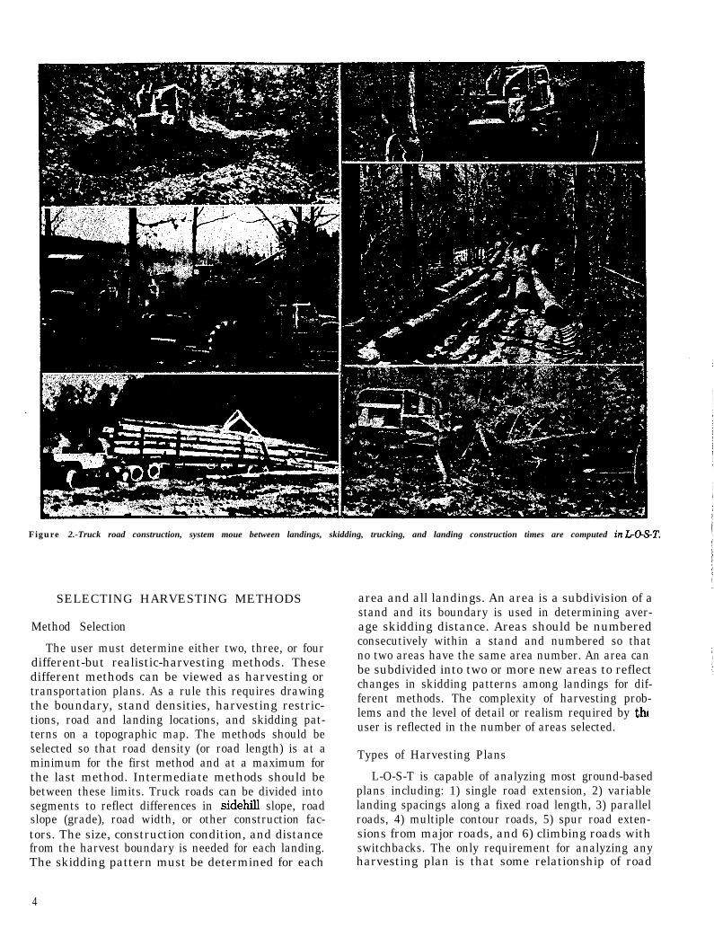
Figure 2.-Truck road construction, system moue between landings, skidding, trucking, and landing construction times are computed inL-O-S-T.

SELECTING HARVESTING METHODS

Method Selection

The user must determine either two, three, or fourdifferent-but realistic-harvesting methods. Thesedifferent methods can be viewed as harvesting ortransportation plans. As a rule this requires drawingthe boundary, stand densities, harvesting restric-tions, road and landing locations, and skidding pat-terns on a topographic map. The methods should beselected so that road density (or road length) is at aminimum for the first method and at a maximum forthe last method. Intermediate methods should bebetween these limits. Truck roads can be divided intosegments to reflect differences in sidehill slope, roadslope (grade), road width, or other construction fac-tors. The size, construction condition, and distancefrom the harvest boundary is needed for each landing.The skidding pattern must be determined for each

area and all landings. An area is a subdivision of astand and its boundary is used in determining aver-age skidding distance. Areas should be numberedconsecutively within a stand and numbered so thatno two areas have the same area number. An area canbe subdivided into two or more new areas to reflectchanges in skidding patterns among landings for dif-ferent methods. The complexity of harvesting prob-lems and the level of detail or realism required by thfuser is reflected in the number of areas selected.

Types of Harvesting Plans

L-O-S-T is capable of analyzing most ground-basedplans including: 1) single road extension, 2) variablelanding spacings along a fixed road length, 3) parallelroads, 4) multiple contour roads, 5) spur road exten-sions from major roads, and 6) climbing roads withswitchbacks. The only requirement for analyzing anyharvesting plan is that some relationship of road

4

Figure 3.-Felling, bucking, skid rood construction, and bunching times are not computed in L-O-S-T.

length and skidding exists between adjacent harvest-ing methods: From a silviculture perspective theseharvesting plans could be for individual tree selec-tion, group selection, diameter limit, financial matu-rity, or clear cuts. Once a cutting practice has beenselected for an area in one method, it must remain thesame in all the remaining methods. More than one dif-ferent cutting practice may be used within a stand orharvest boundary.

OPTIMIZATION METHODOLOGY

Linear Programming Formulation

After the hours required for road construction,landing construction, system move between landings,skidding, and trucking have been calculated for eachmethod, they are utilized in a linear programmingformulation (equations 1 - 6). The formulation deter-

mines the proportion (X) of each method that shouldbe used. The formulation used in L-O-S-T is a slightmodification of McCarl’s (1979) and is also very simi-lar to those developed by Allen (1956) and Chiang(1974).

Maximize: Z = P&o - CC,H, (1)

Subject to: Qo- C&J,,, 20 t4

CXi,h, -Hi 50 (3)

Q” cx=F (4)=m 6)

Hizbi (6)

Qo, Q,, ‘,, Hi ~ 0where: Z = objective function

P = delivered price of the harvested timber (ie. $11,000 board feet)

5

Figure &-Decking, loading, move-in, and unloading times are not computed in LO-S-T.

TOTAL COST

MINIMUM COST POINT

TRUCK ROADCONSTRUCTION

SYSTEM MOVELANDING CONSTRUCTION

SKID ROAD CONSTRUCTIOLOADING E UNLOADING

UCKING

LENGTH OF CONSTRUCTED ROADS (FEET)

Figure B.-Assumed harvest cost relationships with respect to theoptimum location of roads and landings (Note: fixedcosts lines are in an arbitrary order).

Figure C-Relationships among isoqunnts, activity rays, and hapvesting functions.

6

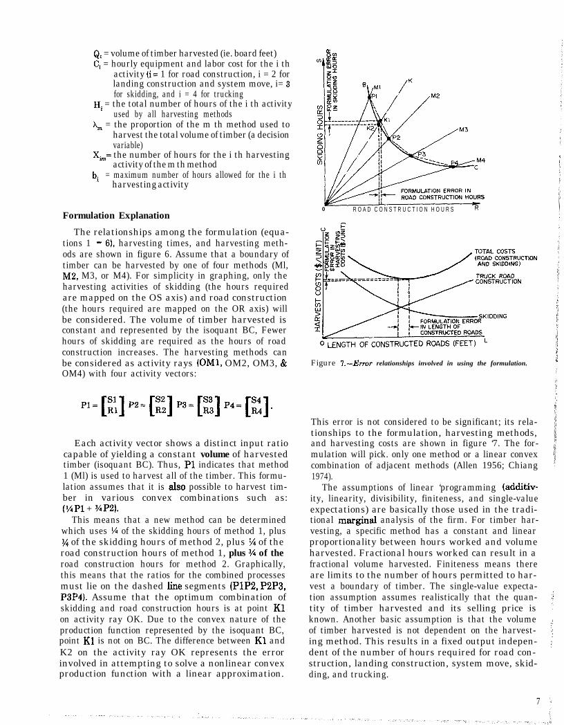
QIt = volume of timber harvested (ie. board feet)Ci = hourly equipment and labor cost for the i th

activity (i= 1 for road construction, i = 2 forlanding construction and system move, i= 3for skidding, and i = 4 for trucking

Hi = the total number of hours of the i th activityused by all harvesting methods

X, = the proportion of the m th method used toharvest the total volume of timber (a decisionvariable)

X,= the number of hours for the i th harvestingactivity of the m th method

bi = maximum number of hours allowed for the i thharvesting activity

Formulation Explanation

The relationships among the formulation (equa-tions 1 - 6), harvesting times, and harvesting meth-ods are shown in figure 6. Assume that a boundary oftimber can be harvested by one of four methods (Ml,M2, M3, or M4). For simplicity in graphing, only theharvesting activities of skidding (the hours requiredare mapped on the OS axis) and road construction(the hours required are mapped on the OR axis) willbe considered. The volume of timber harvested isconstant and represented by the isoquant BC, Fewerhours of skidding are required as the hours of roadconstruction increases. The harvesting methods canbe considered as activity rays (OMl, OM2, OM3, &OM4) with four activity vectors:

Each activity vector shows a distinct input ratiocapable of yielding a constant volume of harvestedtimber (isoquant BC). Thus, Pl indicates that method1 (Ml) is used to harvest all of the timber. This formu-lation assumes that it is also possible to harvest tim-ber in various convex combinations such as:(%Pl + %P2).

This means that a new method can be determinedwhich uses l/4 of the skidding hours of method 1, plus% of the skidding hours of method 2, plus ‘/4 of theroad construction hours of method 1, plus 3A of theroad construction hours for method 2. Graphically,this means that the ratios for the combined processesmust lie on the dashed line segments (PlP2, P2P3,P3P4). Assume that the optimum combination ofskidding and road construction hours is at point Klon activity ray OK. Due to the convex nature of theproduction function represented by the isoquant BC,point Kl is not on BC. The difference between Kl andK2 on the activity ray OK represents the errorinvolved in attempting to solve a nonlinear convexproduction function with a linear approximation.

0 R O A D C O N S T R U C T I O N H O U R S

:TION

Figure I.-Error relationships involved in using the formulation.

This error is not considered to be significant; its rela-tionships to the formulation, harvesting methods,and harvesting costs are shown in figure ‘7. The for-mulation will pick. only one method or a linear convexcombination of adjacent methods (Allen 1956; Chiang1974).

The assumptions of linear ‘programming (additiv-ity, linearity, divisibility, finiteness, and single-valueexpectations) are basically those used in the tradi-tional margi.nal analysis of the firm. For timber har-vesting, a specific method has a constant and linearproportionality between hours worked and volumeharvested. Fractional hours worked can result in afractional volume harvested. Finiteness means thereare limits to the number of hours permitted to har-vest a boundary of timber. The single-value expecta-tion assumption assumes realistically that the quan-tity of timber harvested and its selling price isknown. Another basic assumption is that the volumeof timber harvested is not dependent on the harvest-ing method. This results in a fixed output indepen-dent of the number of hours required for road con-struction, landing construction, system move, skid-ding, and trucking.

7

HARVESTING EXAMPLE PROBLEM

Problem Description

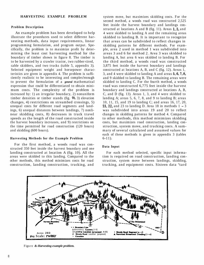
An example problem has been developed to helpillustrate the procedures used to select different har-vesting methods, data input requirements, linearprogramming formulation, and program output. Spe-cifically, the problem is to maximize profit by deter-mining the least cost harvesting method for theboundary of timber shown in figure 8. The timber isto be harvested by a crawler tractor, two rubber-tired,cable skidders, and two trucks (table 5, appendix 3).Selected equipment weight and horsepower charac-teristics are given in appendix 4. The problem is suffi-ciently realistic to be interesting and complex’enoughto prevent the formulation of a general mathematicalexpression that could be differentiated to obtain mini-mum costs. The complexity of the problem isincreased by: 1) an irregular boundary, 2) nonuniformtimber densities or timber stands (fig. 9), 3) elevationchanges, 4) restrictions on streambed crossings, 5)unequal costs for different road segments and land-ings, 6) unequal distances between landings, 7) nonli-near skidding costs, 8) decreases in truck travelspeeds as the length of the road constructed insidethe harvest boundary increases, and 9) restrictions onthe time permitted for road construction (120 hours)and skidding (600 hours).

Harvesting Methods for the Example Problem

For the first method, a woods road was con-structed 350 feet inside the harvest boundary and onelanding constructed at location A (fig. 10). All theareas were skidded to this landing. Compared to theother methods, this method minimizes costs for roadconstruction, landing construction, trucking, and

system move, but maximizes skidding costs. For thesecond method, a woods road was constructed 2,525feet inside the harvest boundary and landings con-structed at locations A and B (fig. 11). Areas 1,3, and4 were skidded to landing A and the remaining areasskidded to landing B. It is important to recognizethat areas can be subdivided to reflect changes inskidding patterns for different methods. For exam-ple, area 2 used in method 1 was subdivided intoareas 3 and 6 for method 2. Area 3 was skidded tolanding A, but area 6 was skidded to landing B. Forthe third method, a woods road was constructed3,875 feet inside the harvest boundary and landingsconstructed at locations A, B, and C (fig. 12). Areas 1,3, and 4 were skidded to landing A and areas 5,6,7,8,and 9 skidded to landing B. The remaining areas wereskidded to landing C. For the fourth method, a woodsroad was constructed 6,775 feet inside the harvestboundary and landings constructed at locations A, B,C, and D (fig. 13). Areas 1, 3, and 4 were skidded tolanding A; areas 5, 6, 7, 8, and 9 to landing B; areas10, 11, 15, and 19 to landing C; and areas 16, 17, 20,21,22, and 23 to landing D. Area 18 in methods 1 - 3was subdivided into areas 19 and 20 to reflectchanges in skidding patterns for method 4. Comparedto other methods, this method minimizes skiddingcosts, but maximizes road construction, landing con-struction, system move, and trucking costs. A sum-mary of several calculated and assumed values foreach of these methods is given in appendix 3 (tables6-11).

Data Input

For each method selected, specific input informa-tion is required on road construction, landing con-struction, system move between landings, skidding,trucking, and equipment costs. Sixteen data “card

Acres: 283Map Scale: 1”:660’

- - Bomd~ry Lin*0 B o u n d a r y Comm ( I - S )0 Landinp Localion (propmod: A-D) I woodsYhdzsagmml(*--/)“f z;ozMd Location (proposed) APumiWstnwnkd

Figure &-Harvesting example problem.

8

types” are required for each analysis of a boundary oftimber to be harvested. An additional card type isrequired if constraints are placed on the number ofhours allowed for any of the pertinent harvestingactivities. These different card types are described indetail in appendix 5. The complete input data used toanalyze the hypothetical example is shown in appen-dix 6. The values shown for average skidding distancewere based on the harvest patterns for the differentareas and landing locations in figures 10 - 13. Aver-age skidding distances were determined using aBASIC program written for use on an HP 9830A’calculator and HP 9864A digitizer. ’

Output Analysis

The computer output for the harvesting exampleproblem is shown in appendix 7. The output consistsof: 1) an echo check of the input data, 2) harvestingtimes and costs, and 3) the linear programming solu-tion and sensivity analysis.

Road construction times and costs, the number ofbank cubic yards, and acres cleared for the road-right-of-way are given for each segment. Road constructioncosts are: $170 for method 1 ($2,565 per mile); $1,061for method 2 ($2,219 per mile): $1,625 for method 3($2,214 per mile); and $2,910 for method 4 ($2,268 permile). The easiest way to modify road constructioncosts without changing the road design or road con-struction equipment characteristics is through theinput variable ROADTY (card type 10, appendix 5).Although guidelines are provided for estimatingROADTY, a value should be selected that gives

‘The use of trade or corporate names is for reader association andconvenience. Such does not constitute an official evaluation, con-clusion, recommendation, endorsement, or approval of any productor service to the exclusion of others which may be suitable.

reasonable cost estimates based on the user’s experi-ence or modeling needs.

Landing construction and system move times andcosts are computed for each landing. Landing con-struction costs are: $56.27 for method 1; $89.64 formethod 2; $118.73 for method 3; and $150.83 formethod 4. The simplest way to influence landing con-struction costs without changing the landing designor landing construction equipment characteristics isthrough the input variable EFFL (card type 12,appendix 5). System move costs are: $0.0 for method1; $101.26 for method 2;.$192.39 for method 3; and$303.78 for method 4.

Skidding times and costs are computed for eachskidder on each area and summarized by area, land-ing, and method. The number of cycles and averagecycle time are also given. The skidding costs are:$28,769.13 for method 1; $18,076.16 for method 2;$15,471.31 for method 3; and $10,950.56 for method4. The easiest way to modify skidding times withoutchanging skidder characteristics, skid load volumes,or skidding distances is through the input variable,AD (card type 13, appendix 5).

In addition to skidding times and costs, averageskidding distance, fixed skidding distance, andweighted actual travel skidding distances are summa-rized by landing and method. In most cases the great-est potential for reducing skidding times is through areduction of average fixed skidding distance. In theharvesting example problem, average skidding dist-ance only decreased from 686 feet for method 1 to 550feet for method 4. However, average fixed skiddingdistance decreased form 4,296 feet for method 1 to759 feat for method 4. This drastic reduction in aver-age fixed skidding distance was largely responsiblefor skidding times decreasing from 659.75 hours formethod 1 to 264.83 hours for method 4. Weightedaverage travel skidding distance is computed by mul-

Harve*l Bolmdafy Linef&eie: 1” 9 660’

TOId ma : 253Total H a r v e s t V o l u m e : 567,500 B o a r d F e e t (#” ht.)

Figure O.-Stand densities and acres for the harvestingproblem.

Landing Construction:Lendinp ot A

Figure lO.-Road, landing, and area locations used in method 1.

tiplying average skidding distance by the skiddingcorrection factor for each area. This product is addedto to the fixed skidding distance on each area andthen multiplied by the volume for that area in orderto obtain a weighted value.

The number of acres and volume of timber har-vested for each method are provided as informationand as checks on the accuracy of data input. Thenumber of acres for each method must be the sameand the volume harvested for each method must bethe same. In this example, 283 acres and 567,500board feet (VI ’ Int.) were harvested for each method.The linear programming formulation requires that anequal volume of timber be harvested in each method.

Trucking times and costs are shown for each truckand are summarized by landing and method. In addi-tion, cycle times and number of loads required foreach truck are given. Trucking costs for each methodare: $17,182.48 for method 1; $17,913.40 for method2; $18,277.16 for method 3; and $18,774.91 formethod 4. In this case the construction of four land-ings and 6,775 feet of woods roads only increasedtrucking costs by $1592.43.

A method summary giving the hours, costs perharvesting unit for each function, total costs, andtotal costs per harvesting unit is provided in the out-put. The total harvesting costs per thousand boardfeet ( ‘/ ’ Int.) for road construction, landing construc-tion and system move, skidding, and trucking are:$81.37 for method 1; $65.62 for method 2; $62.79 formethod 3; and $58.31 for method 4. The hoursrequired for each harvest function considered in L-O-S-T are shown in table I and are used to illustrate anumerical example of the linear programming formu-

10

lation (equations 7 - 16). The formulation can also beseen in the output (appendix 7) as the first iteration ofthe linear programming tableaus.

Table I.--Harvest hours for the four methods

Harvest Method 1 Method 2 Method 3 Method4Function (hours) (hours) (hours) (hours)Road construction 7.86 49.07 75.12 134.65Landing construction

& system move 0.78 2.64 4.31 6.29Skidding 695.75 437.15 374.16 264.83Trucking 429.56 447.83 455.68 469.37

After 18 iterations the optimum linear program-ming solution consisted of 24 ‘JJo of method 3 and 76%.of method 4. The optimum method (not a global opti-mum) used 120 hours of road construction, 5.8 hoursof landing construction and system move, 292 hoursof skidding, and 466 hours of trucking. The linearprogramming solution does not give the exact physi-cal location of the roads, landings, and skidding pat-terns. However, the output Can be used to help locatethe road, landings, and skidding patterns for a newmethod consisting of 24% of method 3 and 76% ofmethod 4. Since 102.2 hours were required to con-struct the road to the end of segment h-i, then 17.8hours (120.0-102.2) or 909 feet of segment i-j can beconstructed. The road should be constructed 2,159feet beyond landing C. Landing D would be located6,034 feet from the harvest boundary; whereas it wasoriginally located 6,775 feet. The skidding patternswould stay the same for landings A and B, and proba-bly C. However, the skidding patterns would changefor landing D. If another computer analysis tieremade in order to obtain a better estimate, then meth-

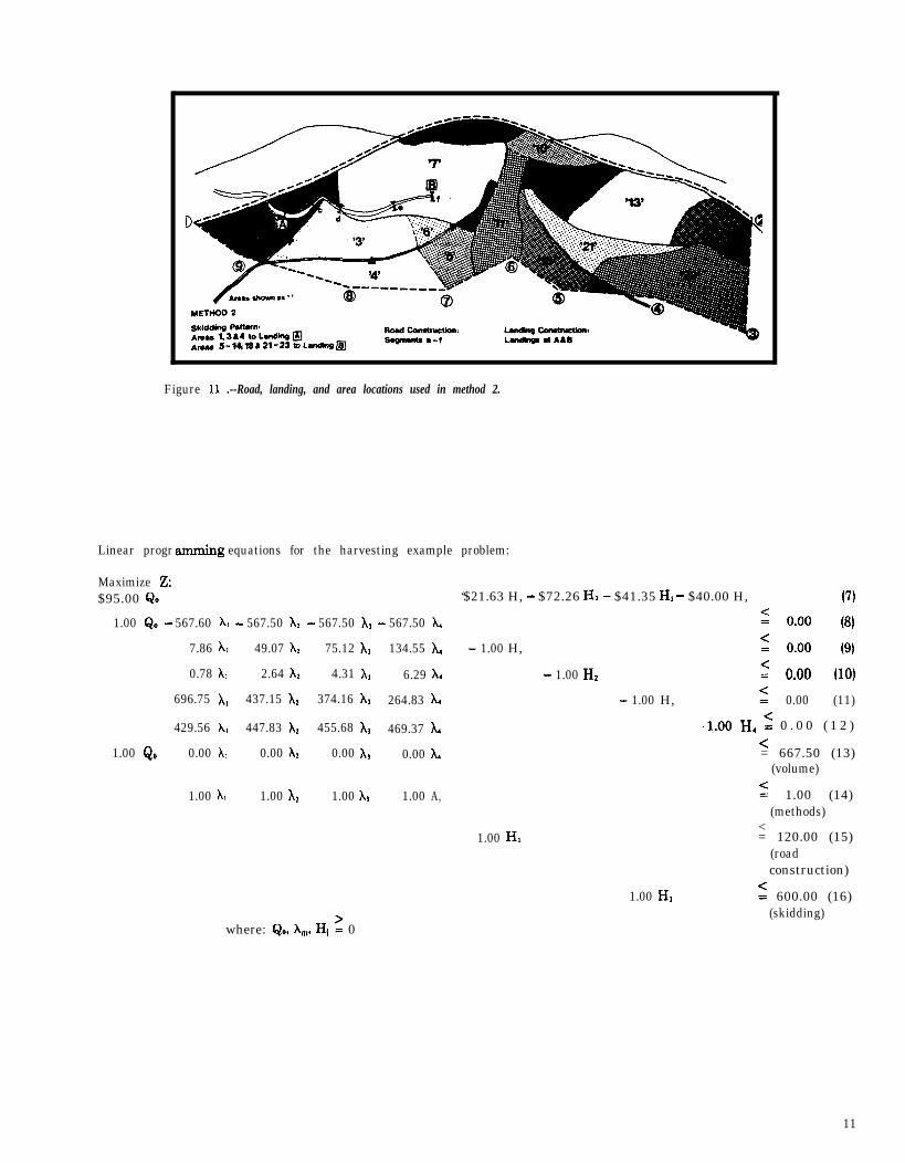
Figure 11 .--Road, landing, and area locations used in method 2.

Linear progr amming equations for the harvesting example problem:

Maximize 2:$95.00 Qo ‘$21.63 H, - $72.26 H2 - $41.35 H, - $40.00 H,

1.00 Q,, - 567.60 Xc - 567.50 At - 567.50 A, - 567.50 A,

7.86 A, 49.07 x1 75.12 A, 134.55 A, - 1.00 H,

0.78 A, 2.64 A, 4.31 A, 6.29 A, - 1.00 Hz

696.75 A, 437.15 XI 374.16 X, 264.83 X, - 1.00 H,

429.56 A, 447.83 A, 455.68 A, 469.37 A,

1.00 Qo 0.00 A, 0.00 x2 0.00 A, 0.00 A,

1.00 x, 1.00 x2 1.00 A, 1.00 A,

2 0.00 (81

f 0.00 (9)5 0.00 (10)2 0.00 (11)

.I.00 H, 2 0 . 0 0 ( 1 2 )<= 667.50 (13)

(volume)

5 1.00 (14)(methods)

<= 120.00 (15)

(roadconstruction)

2 600.00 (16)(skidding)

1.00 H,

1.00 H,

where: Qo, &,,,, Hi 2 0

(7)

11

ods 1 and 2 should be eliminated. Two new methodsshould be selected between the original methods 3and 4. The original method 3 would become the newmethod 1. By keeping two of the original methods,the amount of new input data needed is reduced andthe search area can be systematically analyzed.

Harvesting costs for the optimum method were$59.41 per thousand board feet ( M’ Int.). If the con-straint on road construction (120 hours) were notbinding, then all of method 4 could have been usedand harvesting costs would have been $58.31 perthousand board feet. Binding constraints alwayscause an increase in costs. However, the optimummethod selected by the linear program (24% ofmethod 3 and ‘76% of method 4) is still better than themethod 1 ($81.37), method 2 ($65.62), or method 3($62.79).

The sensivity analysis in L-O-S-T consists of pen-alty costs, shadow prices, and ranges on all the costcoefficients and constraints. The formulation used inL-O-S-T and the original input format of the linearprogram algorithm make it difficult to correlate thevariable codes in the sensivity analysis with the cor-rect harvesting costs and constraints. However,users familiar with sensivity analysis should be ableto interpret these results in L-O-S-T. In this formula-tion shadow prices are always zero because all thetimber can be harvested by the number of hours com-puted for each method. The hourly costs of the har-vesting functions are always non-basic. In this exam-ple, the hourly cost of road construction can increasefrom $21.63 to $64.43 without changing the optimumsolution. This implies that the same road could havebeen constructed to a higher standard or that moreroads should be constructed. The method summarycosts also indicated that more roads and landinns

LIMITATIONS

The linear programming solution calculated in L-O-S-T is not a global optimum or the absolute best of allpossible harvesting methods. The program deter-mines the “best” method based on the methods sup-plied by the user. Equipment interactions resulting inproduction delays are not calculated by the program.The effects of equipment interactions must be sup-plied indirectly by the user through equipment effi-ciency and area difficulty factors. Harvesting costsare calculated only for road construction, landingconstruction, system move between landings, skid-ding, and trucking. While this does not limit theoptimization process, an estimate of total harvestingcosts is not provided.

EXECUTING L-O-S-T

L-O-S-T is written in FORTRAN IV and is beingrun under WATFIV on an IBM 3031 at Auburn Uni-versity. With a modest amount of additional effort,the program could be converted for use on similarcomputer systems. The example problem described inthis report required 264K of storage, used 3.38 sec-onds of CPU time, and cost about one dollar to run.The FORTRAN source statements used in L-O-S-Tare shown in appendix 8. A punched and interpretedsource deck (1,914 cards) can be obtained from: Engi-neering Research Unit, G. W. Andrews Forestry Sci-ences Laboratory, U. S. Forest Service, Devall Street,Auburn Universitv, Alabama 36849. Phone (205) 887-7542, (FTS) 534-4ji8.should be constructed.

Figure l2.-Road, landing, and area locations used in method 3.

12

RESULTS AND DISCUSSION

A two-part methodology has been developed toanalyze user selected harvesting methods. The firstpart of this methodology considers very specific andrealistic harvesting conditions: terrain features,boundary shapes, roads, landings, skidding patterns,and environmental restrictions. Harvesting timesand costs are computed for road construction, land-ing construction, system move between landings,skidding, and trucking. The second part of the metho-dology uses these harvesting times in a linear pro-gramming formulation. The formulation utilizes therelationships among the harvesting methods to esti-mate and select the harvesting procedure havingmaximum profits.

Since the analysis performed by L-O-S-T dependson the harvesting methods selected by the users, it isimportant that users have some knowledge andexperience in developing harvesting plans. Time andeffort spent in selecting realistic harvesting plans willenable the output from L-O-S-T to be used withgreater confidence by managers of harvesting opera-tions.

L-O-S-T does not provide a global optimum witheach computer analysis. Theoretically, the proceduresused would, through repeated computer runs, find theultimate harvesting method having maximum prof-its. L-O-S-T does provide a local optimum and awealth of information for selecting a better harvest-ing method. Searching for the elusive global optimumhas some academic merit; however, selecting feasibleharvesting plans and then systematically quantify-ing, analyzing, and improving them has greater prac-tical applications.

LITERATURE CITED

Allen, R. G. D. Mathematical economics. New York,New York: MacMillan and Company, Ltd.; 1956. p.618 - 632.

Bowan, John K; McCrea, Robert B; Fonnesbeck, CarlI. A method of field design applied to forest roads.Transportation Research Board, NationalResearch Council, National Academy of Sciences,Washington, D.C., Special Report No. 160. In pro-ceedings of Transportation Research Board Work-shop, June 16- 19,1975. p. 186 - 197.1975.

Carter, Michale R; Gardner, R. B; Brown, David B.Optimum economic layout of forest harvestingwork roads. Res. Paper INT-133. Odgen, UT: U.S.Dept. of Agric., Forest Service, IntermountainFor. Exp. Station; 1973.13 p.

Chiang, Alpha C. Fundamental methods of mathe-matical economics. 2d ed. New York, New York:McGraw Hi& 1974. p. 684 - 689.

Corcoran, T. J; Sammis, R. Optimized landing androad spacing. Registry of Computer Programs,American Society of Agricultural Engineers, St.Joseph, MI, Program No. COM 0108,1975.

Dykstra, Dennis Peter. Timber harvest layout bymathematical and heuristic programming. Ph.D.dissertation, Oregon State University, Corvallis,Oregon; 1976.‘299 p.

Gibson, David F; Egging, Louis, T. A location modelfor determining the optimal number and location ofdecks for rubber-tired skidders. Winter MeetingAmerican Society of Agricultural Engineers;December 14 - 17; Chicago, IL. ASAE paper no.73-1534. St. Joseph, MI, ASAE; 1973.14 p.

Goulet, D. V; Iff, R. H; Sirois, D. L. Five forest har-vesting simulation models, Part II: paths, pitfalls,

Figure I%-Road landing, and area locations used in method 4.

13

and other considerations. Forest Products Journal,30(8): p. 18 - 22.1980.

Greulich, Francis E. Average yarding slope and dist-ance on settings of simple geometric shape. ForestScience, 26(2): p. 195 - 202. 1980.

Kirby, Malcolm. Transportation systems and theland use plan: a mathematical programmingapproach. Engineering Technical Report NO. ETR7700-g. Berkley, CA: U.S. Dept. of Agric., ForestService, Pacific Southwest; 1974.17 p.

Koger, Jerry L. Factors affecting the production ofrubber tired skidders. Division of Forestry, Fisher-ies, and Wildlife Development, Tennessee ValleyAuthority, Norris, Tennessee, Technical Note No.B18,55 p. 1976.

Koger, Jerry L. Factors affecting the constructionand cost of logging roads. Division of Forestry,Fisheries, and Wildlife Development, TennesseeValley Authority, Norris, Tennessee, TechnicalNote No. B27,95 p. 1978.

Koger, Jerry L. Transportation methods and costsfor sawlogs, pulpwood bolts, and longwood. Divi-sion of Forestry, Fisheries, and Wildlife Development, Tennessee Valley Authority, Norris, Tennes-see, Technical Note No. B44,34 p. 1981.

Lussier, L. J. Use of operations research in determin-ing optimum logging layouts. Pulp and PaperMagazine of Canada, Convention Issue, 282: p.32-41. 1960. (Woodlands Section Index No.1947(A-2-a))

Lussier, L: J. Planning and control of logging opera-tions. Forest Research Foundation, Universit’eLaval, Quebec, Canada, Contribution No. 8, 135 p.1961.

Matthews, D. M. Cost control in the logging indus-

try. New York, New York: McGraw Hill; 1942.314Pa

McCarl, B. A. Production function-convex approxi-mation. Department of Agricultural Economics,Purdue University, West Lafayette, IN. (unpub-lished lecture handout in Agricultural Economics652) p. 48 - 52.1979.

Miyata, Edwin S. Determining fixed and operatingcosts of logging equipment. General TechnicalReport NC-55. St. Paul, MN: U.S. Dept. of Agric.,Forest Service, North Central Forest ExperimentStation; 1980.16 p.

Newnham, R. M. LOGPLAN-a model for planninglogging operations. Canadian Forestry Service,Department of the Environment, Ottawa, Ontario,KIA OH3. Inf. Rep. FMR-X-77.59 p. 1975.

Nichols, Herbert L. Moving the earth: the workbookof excavation. Second Edition. North CastleBooks. Greenwich, CT. 1962. 21 sections plusappendix.

Peters, Penn A. Spacing of roads and landings to rnin-imize timber harvest cost. Forest Science, 24(2): p.209 - 217.1978.

Peters, Penn A; Burke, J. Boyle. Average yardingdistance on irregular-shaped timber harvest set-tings. Res. Note PNW-178. Portland, OR: U.S.Dept. of Agric., Forest Service, Pacific NorthwestFor. Exp. Station; 1972.13 p.

Suddarth, S. K. Cost minimization in the primarytransport of forest products. Ph.D. dissertation,Purdue University, West Lafayette, Indiana; 1952,66 p.

Weintraub, A; Navon, D. I. A forest managementplanning model integrating silvicultural and trans-portation activities. Management Science, 22(12):p. 1299 - 1309.1976.

14

Appendix l-Harvesting Equations, Data, and Cost.Relationships

HARVESTING EQUATIONS AND DATA

road construction equation: (Koger, equation 3, pg 30, 1978)e

0.5

xl35 [ 1X2/(X3X4) +

T=

x7

where : T = predicted road constructed time in hoursXl = road length in feet

ii:= number of bank cubic yards per 1,000 feet= slope correction factor estimated by:

of road length

21.000 - (% road slope/lOO) - 0.0001952 (%

note: % road slope (+, -> is in direction

road slope/lOO)

of road construction

x4 = net horsepower of crawler tractor (Table 1 2, Appendix 4)X5 = number of acres of cleared road width per 1,000 feet of road length

(Al)

x6 = road construction difficulty factor with suggested values of:10 for high volume truck road or low volume road constructed

adverse conditions500 for low volume truck road constructed under average

conditions1,000 for low volume skid road constructed under average

conditions2,000 for upgrading existing low volume skid road under average

conditions3,000 for low volume landing constructed under average conditions

note: intermediate values (ie. 520, 750) can be used

x7 = (equipment availability)(equipment utilization), with suggestedvalues of:0.50 for low availability and utilization0.85 for average availability and utilization0.95 for high availability and utilization

note: only the variables Xl, X4, x6, and Xi’ are required as user suppliedinputs . The variables X2, X3, and X5 are calculated by the program.

.

16

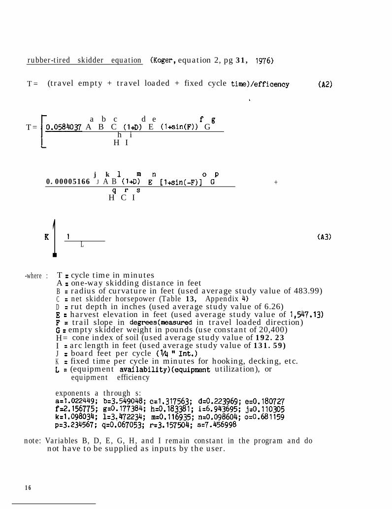
rubber-tired skidder equation (Koger, equation 2, pg 31, 1976)

T = (travel empty + travel loaded + fixed cycle tim)/efficency (A21

.

T=a b c d e f g

A B C (l+D) E (l+sin(F)) Gh i

H I

j k 10.00005166 J A B (1-a~ En WsinMWO Gp +

q r sH C I

K 1 1L

(A31

-where : T = cycle time in minutesA = one-way skidding distance in feetB = radius of curvature in feet (used average study value of 483.99)C = net skidder horsepower (Table 13, Appendix 4)D = rut depth in inches (used average study value of 6.26)E = harvest elevation in feet (used average study value of 1,547.13)F= trail slope in degreestmeasured in travel loaded direction)G = empty skidder weight in pounds (use constant of 20,400)H= cone index of soil (used average study value of 192.23I = arc length in feet (used average study value of 131.59)J = board feet per cycle (l/4 *( Int.)K = fixed time per cycle in minutes for hooking, decking, etc.L = (equipment availability)(equipment utilization), or

equipment efficiency

exponents a through s:a=l,022449; b=3.549048; ~~1.317563; dz0.223969; ez0.180727fz2.156775; gsO.177384; hz0.183381; iz6.943695; j=O.l10305k=1.098034; 1~3~472234; m=0.116935; n=0.098604; o=O.681159p&234567; q=O.O67053; r=3.157504; s=7.456998

note: Variables B, D, E, G, H, and I remain constant in the program and donot have to be supplied as inputs by the user.

16

Table l.--Observed skidding volumes by horsepower*

Horsepower

VOLUME PER CYCLE WHEN MEASURED AS:Pounds Board Feet:+" Int. Cubic Feet Cords

LOW High Mean Low High Mean Low High Mean Low High Mean

70 2,205 7,080 5,266 87 617 410 29 117 83 0.3 1.21 0.90

80 3,141 7,129 5,278 233 741 471 43 120 81 0.54 1.21 0.90

92 4,032 6,921 4,987 350 666 464 67 108 82 0.69 1.18 0.85

94 815 19,188 8,124 23 2,403 861 14 294 119 0.14 3.28 1.39

112 2,983 25,450 8,416 141 2,260 715 51 361 128 0.50 4.35 1.44

120 5,005 20,226 12,822 5O3 2,142 1,334 al 310 199 0.86 3.46 2.19

147** 4,120 7,095 5,468 419 776 575 71 122 94 0.70 1.21 0.93

165++ 4,808 5,503 5,155 445 522 484 83 95 89 0.82 0.94 0.88

l (Koger, Table 6, pg 22, 1976)

** Did not observe &en stand conditions permitted high volu& skidding.

trucking equation

The following equation is used to calculate truck cycle time from landingsto the delivery point (mill).

Y. =o + 0 +l j - -’s;

‘i X i + Ki

J

where: Y. i =1J

FjJ

CEj’l+Ci)‘/2 (Lj(l+ciW2

round trip truck time in hours from the i th landingfor the j th truck

o=

sj =F . =

Jxi =

E . =J

ci =

one-way distance in miles over roads outside theharvest boundaryaverage empty travel speed in miles per hour for the j th truckover sections outside the harvest boundary (woods to mill)average loaded travel speed in miles per hour for the j th truckover sections outside the harvest boundary (woods to mill)distance in miles from beginning of harvest boundary tothe i th landingempty travel speed in miles per hour over the woods road forthe j th truckratio of ending travel speed to beginning travel speed_ -

L.as measured from beginning of harvest boundary to the i th landing

J= loaded travel speed in miles per hour over the woods road for

the j th truck

Kj= fixed time per cycle in hours for the j th truck

(A41

trucking data

Table 2.-- Average truck speed versus road type*

Average AverageEmpty LoadedSpeed Speed

Type of Road (mph) (mph)

woods 8 4Gravel 16::3

5.3513.89

Two-lane black top 38.76 33.78Interstate 55.00 45.82city 23.97 21.44

3 (Koger, Table 1, pg 5, 1981)

18

Table 3 .--Load characteristic for trucks hauling logs(or tree-length stems)*

Truck Description

Average Average Average AverageNumber Length VolurIE Volume

of logs (feet) (Doyle) (l/41f Wt.)

Single-Axle (1.5-ton) 8:0

13.6 1,313 1,752Tandem-Axle (1 drag) 12.9 1,937 2,584

Tandem-Axle (2-ton) 25 13.0 2,018Tri-Axle (1 drag) 15.2 2,643 ;';2Four-Axle (&drag) 22 11.7 3,276 4:370Tractor-Trailer (logs) 43 14.5 3,868 5,160Tractor-Trailer (stems) 35 36.9 4,222 5,632

3 (Koger, Table 2, 6,pg 1981)

Table 4 .--Load characteristics for trucks hauling pulpwood(bolts, 21-foot stems, or tree-length stems)*

Truck Description

Single-Axle (0.75-ton)Single-Axle (l-ton)Single-Axle (1.5 ton)Tandem-Axle (I drag)Tractor-TrailerTandem-Axle (2-ton)Tri-Axle (I drag)Tractor-Trailer

Type of Load

Pulpwood bolts (5' 3")Pulpwood boltsPulpwood boltsPulpwood boltsTree-length21-foot stems21-foot stemsPulpwood bolts

Averagevqaxne(cords)

1.52.14.6

27'

* (Koger, Table 3, pg 6, 1981)

HARVESTING COST RELATIONSHIPS

Landing Construction and System Move

In the linear programming formulation, landing construction and system move

times and costs are considered together. The following equation is used to com-

pute a weighted time for landing construction and system moving.

WH= (SL + SM)/(HL + HM) (A5)

19

Where: WH = weighted number of hours for landing construction andsys tern move

- sum ofgi 5 sum ofHL = hourlyHM= hourly

landing construction costs for this methodsystem move costs for this methodlanding construction costssystem move costs

Multiple Equipment

In many cases multiple crawler tractors, skidders, or trucks may be used.

For example, two rubber-tired cable skidders may be used on the same boundary to

skid trees to the landings. Equation A6 is used to compute total time under

these conditions. This equation is used for multiple equipment involved in road

construction, skidding, or trucking, but not for landing construction. Only one

crawler tractor is allowed to construct landings, although two or more are

involved in road construction.

T = 11 + 1 + . . . . + 1- -Hl H2 Hn

(A61

where: T =H, =

H2 =

H, =

hours required if all equipment (ie. skidders) uorked togetherhours required if this harvesting activity were done entirely bythe first machinehours required if this harvesting activity were done entirely bythe second machinehours required if this harvesting activity were done entirely bythe last machine

Equipment Interactions and Efficiency

Equipment interactions resulting in production delays are not directly con-

sidered. However, an equipment efficiency factor which considers utilization is

available and can be used to model indirectly the effects of delays caused by

equipment interactions. Equipment efficiency can be estimated or calculated by

the following equation.

E = AUwhere: E = equipment efficiency (decimal value greater than 0)

A= equipment availability (decimal)u = equipment utilization (decimal)

(A71

20

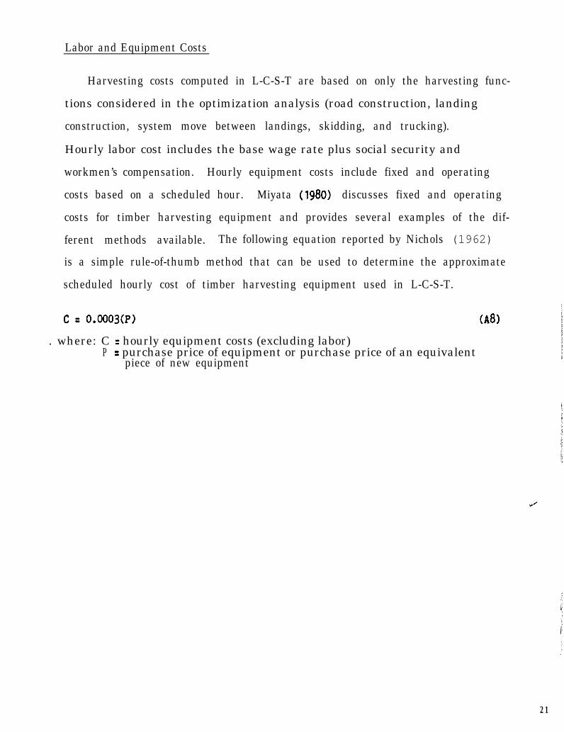
Labor and Equipment Costs

Harvesting costs computed in L-C-S-T are based on only the harvesting func-

tions considered in the optimization analysis (road construction, landing

construction, system move between landings, skidding, and trucking).

Hourly labor cost includes the base wage rate plus social security and

workmen’s compensation. Hourly equipment costs include fixed and operating

costs based on a scheduled hour. Miyata (1980) discusses fixed and operating

costs for timber harvesting equipment and provides several examples of the dif-

ferent methods available. The following equation reported by Nichols (1962)

is a simple rule-of-thumb method that can be used to determine the approximate

scheduled hourly cost of timber harvesting equipment used in L-C-S-T.

c= O.o003(P> (AN

. where: C = hourly equipment costs (excluding labor)P = purchase price of equipment or purchase price of an equivalent

piece of new equipment

J

21

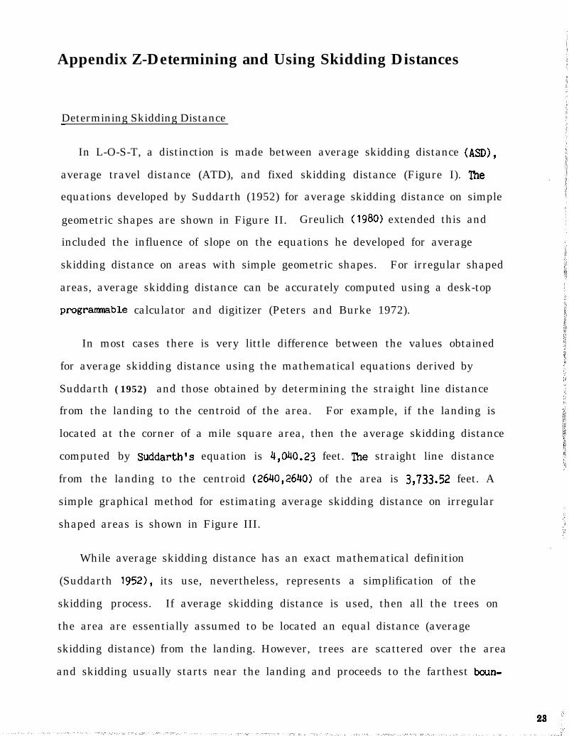
Appendix Z-Determining and Using Skidding Distances

Determining Skidding Distance

In L-O-S-T, a distinction is made between average skidding distance (ASD),

average travel distance (ATD), and fixed skidding distance (Figure I). ‘Ihe

equations developed by Suddarth (1952) for average skidding distance on simple

geometric shapes are shown in Figure II. Greulich (1980) extended this and

included the influence of slope on the equations he developed for average

skidding distance on areas with simple geometric shapes. For irregular shaped

areas, average skidding distance can be accurately computed using a desk-top

programmable calculator and digitizer (Peters and Burke 1972).

In most cases there is very little difference between the values obtained

for average skidding distance using the mathematical equations derived by

Suddarth (1952) and those obtained by determining the straight line distance

from the landing to the centroid of the area. For example, if the landing is

located at the corner of a mile square area, then the average skidding distance

computed by Suddarth’s equation is 4,040.23 feet. The straight line distance

from the landing to the centroid (2640,264O) of the area is 3,733.52 feet. A

simple graphical method for estimating average skidding distance on irregular

shaped areas is shown in Figure III.

While average skidding distance has an exact mathematical definition

(Suddarth 1952), its use, nevertheless, represents a simplification of the

skidding process. If average skidding distance is used, then all the trees on

the area are essentially assumed to be located an equal distance (average

skidding distance) from the landing. However, trees are scattered over the area

and skidding usually starts near the landing and proceeds to the farthest boun-

dary of the harvest area. A more accurate estimate of skidding cycle time can

be obtained by integrating the skidding equation (A31 over the range of

skidding distances. Similarly, using an average skidding cycle volume rather

than the range of cycle volumes causes equation A3 to underestimate

skidding times. In L-O-S-T, users have the options of using average values for

skidding distance and volume or their ranges. For simplicity reasons, the

simplifed version (A101 of the skidding equation will be used to illustrate the

integration procedures (All) available in L-O-S-T, given below.,

Y = travel empty time + travel loaded time + fixed time

1.022 1 .og8 0.11Y= 0.0027(X) + 0.00088(x) (VI +K

where: Y = cycle tima in minutes for articulated, four-wheel drive,rubber-tired skidders in the 70 to 130 horsepower range

X = one-way skidding distance in feetv= cycle volume in board feet (14 Int.); must be reasonable for

skidder size and skid trail conditions (Table 1, Appendix 1)K = assumed fixed time (minutes) per cycle for hooking, decking,

/

b 1.022 b d 1 .og8 0.11Y = 0.0027 (Xl dx + 0.00088 (Xl (VI dxdv

b-a a //(b-a)(d-c) a c

+K

where: Y = skidding cycle time in minutesa = lower limit on skidding distance in feetb = upper limit on skidding distance in feet

- lower limit on skidding volume in board feet (WI Int.):I- upper limit on skidding volume in board feet ( l/411 Int. )x = skidding distance, feetv= skidding volume, board feet (l/4*’ Int. >

d x = derivative of Y with respect to Xd v = derivative of Y with respect to VK= fixed time per cycle in minutes for hooking, decking, etc.

(A91

(A101

etc.

(All)

Actual Travel Distance

Due to terrain features (steep slopes, streams, rocks, soft ground) and to

stand characteristics (large stumps, dead snags), the distance actually traveled

by the skidder from the landing to the tis is rarely ever equal to the

24

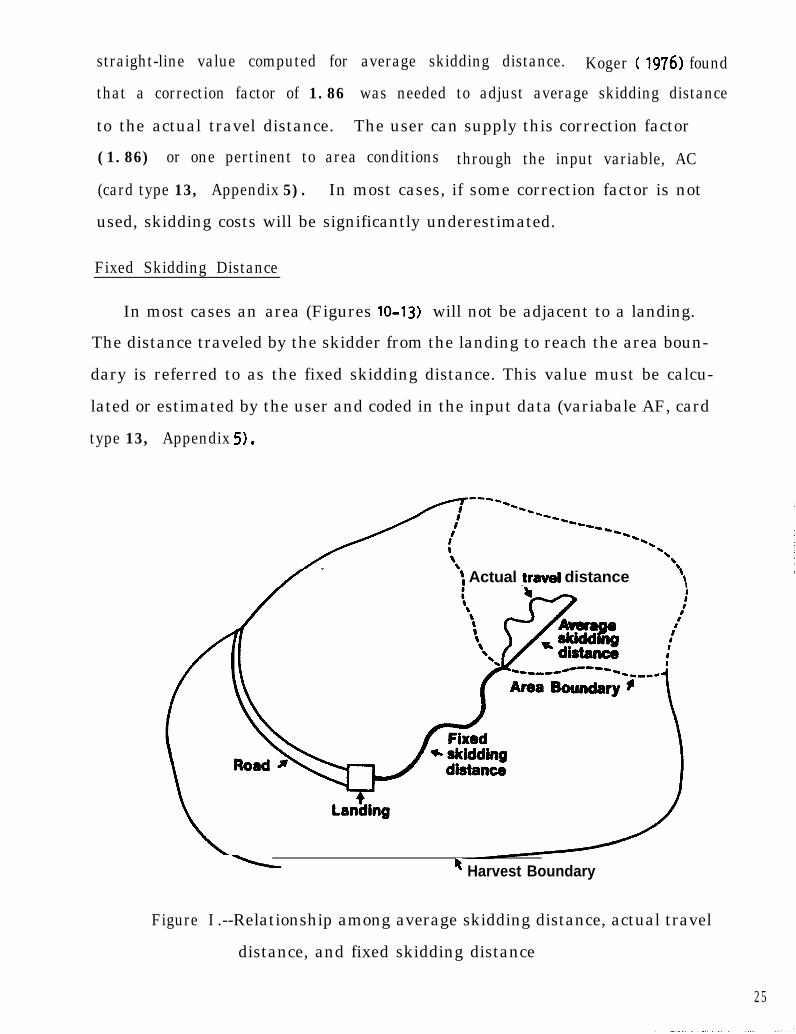
straight-line value computed for average skidding distance. Koger ( 1976) found

that a correction factor of 1.86 was needed to adjust average skidding distance

to the actual travel distance. The user can supply this correction factor

(1.86) or one pertinent to area conditions through the input variable, AC

(card type 13, Appendix 5). In most cases, if some correction factor is not

used, skidding costs will be significantly underestimated.

Fixed Skidding Distance

In most cases an area (Figures lo-131 will not be adjacent to a landing.

The distance traveled by the skidder from the landing to reach the area boun-

dary is referred to as the fixed skidding distance. This value must be calcu-

lated or estimated by the user and coded in the input data (variabale AF, card

type 13, Appendix 5).

: Actual pml distance 88I

’ Harvest Boundary

25

Figure I .--Relationship among average skidding distance, actual travel

distance, and fixed skidding distance

AVERAGE SKIDDING DISTANCE (ASD)FOR SIMPLE GEOMETRIC SHAPES

CIRCLE (Suddorth 1952) CIRCULAR SEGMENT (Suddarth 1952)

RIGHT TRIANGLE (Suddarth 1952) ANY TRIANGLE (Peters 1978)

L a n d i n g -

RECTANGLEBuddarth 1952)

Where. In = natural log. base e : tan = tangent : arcton = arctangent

Figure II. --Average skidding distance equations for areas with simple

geometr ic shapes

26

MAP BOUNDARY

e---aI<wR;S;----4

/’\I

II

:I

?BOUNDARY i\

\\\ HARVEST\\ AREA\ti'4, LANDING 1

----,- c-----------1, 0'-0)

SMALL PLUM BOB

STEP 1: DETERMINE HARVEST BOUNDARY ANDLANDING LOCATION.

STEP 2: SEPARATE HARVEST AREA FROM MAPBY CUTTING ALONG HARVESTBOUNDARY LINE.

STEP 3:MAKE TWO SMALL HOLES NEARMARGIN OF HARVEST BOUNDARY(AGB). SEPARATE FROM LANDINGBY ABOUT l/3 BOUNDARY CIRCUM-FERENCE.

STEP4: PLACE A NEEDLE IN HOLE AT LOCA-TION (A) AND MAKE SURE THATHARVEST AREA CUTOUT ROTATESFREELY ABOUT THE NEEDLE AXIS.ATTACH A SMALL PLUM BOB TO NE-EDLE AND MARK PLUM LINE ONCUTOUT. REPEAT THIS PROCESS AT@CATION (8).

STEP 5: THE CENTROID -OF THE HARVESTAREA WILL BE AT THE INTERSEC-TION OF THE TWO PLUM BOB LINES(C). MEASURE THE DISTANCE FROMPOINT C TO THE LANDING WITH ARULER. THIS DISTANCE MULTIPLIEDBY THE MAP SCALE WILL GIVE ACLOSE APPROXIMATION OF AVERAGESKIDDING DISTANCE~ASD).

LANDING

Figure III.--Graphic method for determining average skidding distance

when landing is on boundary edge27

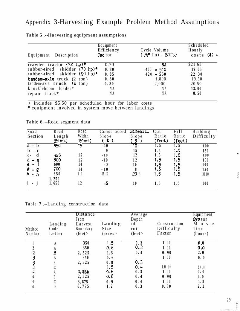
Appendix 3-Harvesting Example Problem Method Assumptions

Table 5 .--Harvesting equipment assumptions

EquipmentEfficiency

Equipment Description Fat tor

crawler tractor (72 hp)* 0.70rubber-tired skidder (70 hp)* 0.80rubber-tired skidder (90 hp)* 0.85tandem-axle truck (2 ton) 0.80tandem-axle truck (2 ton) 0.80knuckleboom loader* N Arepair truck* N A

Cycle Volume<MQt Int . Bdft)

400 - 5:4 2 0 - 550

1,8002,000

N AN A

ScheduledHourly

costs ($1 +

$21.6319.0522.3019.5020.5013.008.50

+ includes $5.50 per scheduled hour for labor costs* equipment involved in system move between landings

Table 6 .--Road segment data

R o a d R o a d Road Constructed Sidehill Cut Fill BuildingSection Length Width Slope Slope Rat i o Rat i o Difficulty

(feet> (feet> (%Ia- b 2: 3; -10 '1; )

(feet> (feet>1.5 1.5 100

b - c -8 15 1.5c- d

E15 -10 12 1.5 1:;

150100

d -e 15 -10 1 2 150e- f 600 14 -8 10 1:; ::; 100ff-i 1;

700 14 -10 8 1.5 1.5 150650

1,25012 13 -15 -12 20 15 ::5" ::: 100 100

i - j 1,650 12 -6 10 1.5 1.5 100

Table 7 .--Landing construction data

MethodNumber

LandingC o d eLetter

Distance Average EquipmentFrom Depth Sys ternHarvest Landing of Construction M o v eBoundary Size cut Difficulty T i m e(feet> (acres> (feet> Factor (hours)

1 A2 A2 .B

:AB

tCA

tBC

4 D

350 5350 A:6

2,525 1.5350 0.6

2,525 0.8

3,875350 x2,525 0:s3,875 0.96,775 1.2

0.3 1.00 0 00.3 1.00 0:o0.4 0.90 2.0

0:4 E

1.00 0.0

0.90 1.00 2.0 1.80.3 1.00 0.00.4 0.90 2.00.4 1.00 1.80.3 0.80 2.2

4

29

Table 8 .--Skidding data for method 1

Average Fixed FixedArea Area Skidding Skidding Trail Cycle

Landing Area Volume Size Distance Distance Slope TimeCode Code (Q+Ynt> (acres) (feet) (feet> (%I Onin>

A 1 65,000 26 485 0 5A 70,000 28 1,005 265 ;A

240,000 16 525 2,080

r:

A

7"

22,500

459

415 3,700 -5 3

A go, 000 1,180 1,200 -10A 8 4,000 22:

4,000 -8 9'A 9 15,000 10 3,000 -10 11A 10 12,000 8 285 4,950 -2 11A 11 24,000 16 1,095 4,550 5 11

A 12 16,000 16 625 5,050 10A :z 27,000 2 7 990 6,230 10 1:A 15,000 15 570 8,000 5 13A 18 26,000 13 520 5,740 15A 21 30,000 15 1,095 5,050 12 ;A 6,000 170 7,700 10A 105,000 900 7,225 10 z


Average Fixed FixedArea Area Skidding Skidding

Landing Area Volume Size Distance Distance 2;: Cyc1eTim!Code Code (WInt> (acres) (feet) (feet> ($1 bin)

A 1 65 000 26 0 5 7

A 23

82: 40

265A 43 ; h;B 22:500

169 :;

2,080 2 ::10 7

Bii

12,500 190go"

12

B 710 :

go, 000 455 630 0 -2B 4,000 2285 CE

1,300 -8 ii 15,000 990

12,00010 8

24,000 161,680

-10 -10 11 11

B 11B

::

16,000 16 YE1,290 -21,780 5 1:

B 27,000 27 990 10B 14 2,67018

15,000 570 5,050 10 ;;B 26,000 ;; 520 2,080 5B 2 3”61g; 15 1,095 1,880 15 99

BB 23 105:OOo 3: 170 3,660 12900 4,260 10 5"



Landing Area Volume Size Distance Distance Slope TiUECode Code (WInt) (acres> (feet) (feet) (46) Onin)

A 1 65,000 26 485 0 5A 57,500 23 820 265

::A t 40,000 16 525 2,080 2 7

B 22,500 ; 415B ii 12,500 '90 iii: 1012 s

B ii go, 000 45 630 0 -2B 4,000 2 zz; 1,300 -8 ;B 9 15,000 10 990 -10 11C 10 12,000 8 285 790 -10 11C 11 24,000 16 1,095 -2 11C 12 16,000 16 625

30:5 13

C 13 27,000 27 990 1,390 10 13C 14 15,000 570 3,660 10 13

C 18 26,000

1;

520 790C 21 30,000 15 1,095 300 1: x

C 22 6,000 3: 170 2,480 12C 23 105,000 900 2,870 10 z



Landing Area VoluuE? Size Distance Distance Slope TiltECode Code (WInt) (acres) (feet) (feet) (%I bin)

A 1 65 000

;p;

26 405 0 5 7A

223 820 265

A 16 2,080 ;BB ii

22;500E y;

12,500 ii '90 iii: 12 ::

B ii go,ooo 45 630 0B 4,000 2 1,300 2 ;B 9 15,000 10

1,095 g;990 -10 11

: 10

1:

24,000 12,000 16 8 790 0 -10 -2 11

C 6,000 6 490 :;C

:;10,000

37270

z: 1;

D 37,000zii:

500 1:D 17 15,000 1; 13

D 20 16,000 '2 335 2,noOD 21 30,000 15 1,170 200 43 x

D 22 6,000 3: 170 2,820D 23 105,000 720 150 z

Appendix 4-Equipment Specifications

Table 12 .-Equipment horsepower and weight characteristicsfor selected crawler tractors

EquipmentMake &Model

Case 3504508501450

Caterpillar D"f-;;

D5-DDD6-DD

John'Deere JDJD;$

JD550

International TD-7EPSTD-8E-PSTD-15c-PS

Kormtsu D'+5A-1

zz

Massey-Ferguson MFE

MFSWB

EquipmentHorsepower(net engine)

3 9

z130

FE105140

z;72

657 8

140

90

110 140

6585136

EquipmentWeight(bare, pounds)

%O 05

13:OOo23,800

l~,~O13,99019,20024,000

8,16011,60012,300

10,45913,83424,153

18,340

22,200 28,220

14,700

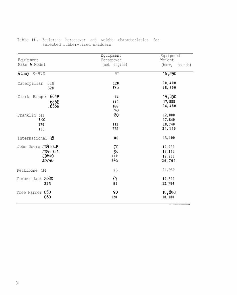
Table 13 .--Equipment horsepower and weight characteristics forselected rubber-tired skidders

EquipmentMake & Model

Athey S-97D

Caterpillar 518528

Clark Ranger 664B666~

. 668~

Equipment EquipmentHorsepower Weight(net engine) (bare, pounds)

97 l6,250

120 20,400175 28,300

82 15,890112166

17,85524,480

Franklin 531132170185

International ~8

John Deere JD440-BJD540-AJD640JD'i'40

io” 12,00017,840

112 18,740775 24,140

86 13,100

'9::12,25016,150

110145

19,90026,700

Pettibone 100 93 14,950

Timber Jack 208D 67225

12,30092 12,784

Tree Farmer C5D 90C6D

15,890120 18,180

34

Appendix &Data Card Types

The following 17 data card types are used in L-O-S-T to describe organizedinput data for the harvesting methods, areas, road segments, landings, andequipment. Unless otherwise stated, all input data is to be right justified.Input variable names beginning with INTf3GER letters (I,J,K,L,M, or N) do notrequire decimal points. Input variable names beginning with REAL letters (A-H,& O-Z) do require a decimal point in the input field location shown. Althoughharvest volume units of pounds, l/4” Int. board feet, cubic feet, or cords may beused, once a unit has been selected it must be used throughout the analysis.The input data for the harvesting example shown in Appendix 6 should be usedto supplement the data card type descriptions given below.

Card Type 1: (required; one card)

64 cc/-I ATITLEO harvesting problem title--_I- w-w


2 cc

'-'

5 ccu NDZR

7 8cc/// NSKD- -

10 11 cc/// NTRK- -

13 cc/-I ICTRAT

15 cc?l-1

17 cc/,I,

I L P A N A

L P C D E

number of methods analyzed(minimum of 2 and a maximum of 4)

number of crawler tractors (l-5)

number of rubber-tired, cable skidders(l-10)

number of trucks (l-10)

number of user supplied constraints(O-4); allows limits on number ofhours permitted for harvestingfunctions considered

linear programming option code:= 0 if linear prograazning analysis

is performed= 1 if linear programming analysis

is not performed

= 0 if no intermediate matrices areprinted; the normal case

= 1 if intermediate matrices areprinted; is helpful in understandingsensivity analysis

36

Card Type 3: (squired; one card)

1 cc/-,

/3/ / / / / / / / /12 cc/, - - - - - - - - I

1 4 18 mcc/ / / / /./ / /- - - - - - -

26 28 cc12? / / / / / /- - - - A - -

35 cc,3; / / / /,--A-

IUNIT

HARVOL

PRODPC

SYSMHC

DFTBTM

Type 4: (required; one card for

4 cc/'/ / / /---A

6 9 cc1 /./ / /- - - -

14 16/'J / / / / /-,-I-,

; NDZR cards required;each crawler tractor building roadscards adjacent)

DZRHPO net horsepower of crawler tractor;(Table 12, Appendix 4)

DZREFO crawler tractor efficiency (ie. 0.80)

ccDZRHCO hourly crawler tractor and operator

cost ($/hr)

Type 5: (required; one card forcards adjacent)

4 cc/'/ / / /---I XDHPO

11 cc/T / / / / /----,A smwT( 1

/7 / /16 cc/-I,- SUXFO

36

unit code for volume;= 1 for pounds= 2 for 1/4" Int. board feet= 3 for cubic feet= 4 for cords

total volume of harvested timberin same units as coded for IUNIT

selling or delivered price in normalselling units tie. $/l,OOO board feet)

hourly cost ($/hr) to move pertinentequipment to the next landing; not anhourly move-in cost

distance in miles from mill to'harvestboundary or start of constructed woods'roads (can be zero if analyzing truckingwithin harvest boundary)

each skidder; NSKD cards required;

net skidder horsepower;(Table 13, Appendix 4)

weight of unloaded skidder in pounds;(Table 13, Appendix 4)

skidder efficiency (ie. 0.75)

18 21 23 cc/ / / /./ / /_I----- s(DHC ( ) hourly skidder and operator cost ($/hr)

Card Type 6: (required; one card for each truck; NTRK cards required;cards adjacent); note: travel speeds must be > 0.

A / /4 cc/--L-

6 9 cc/ / /./ /_I---

14 cc1’: / / /m-z-

1 6 19 cc/ / /./ /--c-

,‘: / /24 cc/,-A-

26 29 cc/ /./ / /--we

31 38 40 cc/ / / / / / / /./ / /_)---------

42 45 47 cc/ / / /./ / /m-m---

lKTENw( >

llmAJw( >

TKTEMD()

TKTLWDO

TKPTPC ( )

TKEFO

TKVOL( )

TKHCO

empty truck travel speed in mph overnon-woods road (Table 2, Appendix 1)

loaded truck travel speed in mph overnon-woods road (Table 2, Appendix 1)

empty truck travel speed in mph overwoods road (Table 2, Appendix 1)

loaded truck travel speed in mph overwoods road (Table 2, Appendix 1)

fixed time per cycle in minutes; caninclude delays, stops for fuel, etc.

truck efficiency (ie. 0.80)

average truck volume (Tables 3 & 4,Appendix 1); same units as IUNIT incard type 3

hourly truck and operator cost ($/hr)

ad type 7: (required; one card for each method; NMETH cards required;cards adjacent)

1 cclJ IMmio method number (l-4)

4 cc//I- - IRDSEG() number of road segments for this method

(O-20)

7 ccLi ILANDN() number of landings for this method

(1-N

Type 8: (required; one card for each landing for each method;cards adjacent)

method number--not number of methods(l-4)

3 7

4 cc‘-’

7 cc///--

10 cc///- -

JNA


1 cc'-'

m-~-A me-- 4n- I---..1 -e-i. --- ---2 O-- each road segment for each method;l;ara lype IV; (reyurreu; UIlt: USI-u LUIcards adjacent)

1 7 cc/ / / 1 / / 1.1 ROAJXL----m-s length of road segment in feet; if

there are no road segments code a0 (zero) in card coluum 6 and thenskip other variables on this card type

landing number--not number of landings(l-8)

number of areas for this landing(l-25); not area code number

maximum value of any area code numberfor this landing; is equal to JNA onlyif areas are numbered consecutively

control card which follows the lastcard type 8 and must have a 0 (zero>coded in card column 1

9 12 cc/ / 1.1 1- - - -14 18 cc

/ / / 1 1.1---me

ROADSW

ROADSP

20 24 cc/ / / / 1.1 ROADSS---we

26 28 30 cc/ / /./ / / ROADCR- - a - -

32 34 36 cc/ / /./ / / ROADFR- - - - -

38 42 cc/ / / / /./ ROADTY--m-w

segment road width in feet

percent slope (+,-I or road segment indirection of construction

percent slopeadjacent road

(+ only) of side-hill

cut ratio; rise in cut per 1 foot ofbase (ie. 1.50)

fill ratio; drop in fill per 1 foot ofbase (ie. 1.50)

road construction difficulty code;= 10 for road constructed underadverse conditions or for high volumetruck traffic

= 500 for road constructed under averageconditions

= 1000 for road constructed underfavorable conditions

38

= 2000 for road constructed undervery favorable conditions, or theup-grading of an existing road

= 3000 for landing constructed underaverage conditions

note: intermediate values (ie. 520, 760)can be used; trial and errortechniques may be required to obtaindesired or expected times and costs


1 cc/.l ILDZR input order number of crawler tractor

in card type 4 that will be used toconstruct all landings (ie. if thesecond crawler tractor in card type 4 isused, then code a 2 in card column 1);only one crawler tractor is permittedto construct landings

Card Type 12: (required; one card for each landing for each method; cardsadjacent; input all landings for first method, then alllandings for second method, etc.)

DSFTBO distance in feet this landing is fromharvest boundary as measured alongwoods road

13 cc,'"/ /JJ- - ACRESL landing size in acres

15 18 cc/ / /./ /- - - -

20 23 cc/ /./ / /e--w

CUTL

EFFL

average depth in feet of earth removedin constructing this landing

landing construction difficulty factor;must be greater than 0.0; suggest:= less than 1.00 for difficult sites= 1 .O for average sites= greater than 1 .O for favorable sites

29 cc,‘F / / / /,,-I- SYSMHR number of hours required to move

equipment to this landing; not a move-intime, but a system move between landingtime; should be 0 (zero) for the firstlanding

Card type 13: (required; one card for each area for each method;cards adjacent)

1 cclJ method number

39

3 cc'-'

5 cc///- -

6 14 cc/ / / / / / / / /./- - - - - - - - -

15 20 cc/ / / / / /./- - - - - -

21 28 c~/ / / / / / / 1.1- - - - - - - -

36 cc/"9/ / / / / / /' /, , - - - - - A

37 44 cc/ / / / / / / /./- - - - - - - -

46 48 50 CC/ / /./ / /--m-B

56 cc/5'/ / / / /,---'

58 61 cc/ /./ / /- - - -

ILN

IAN

A C

landing number

area code number

area volume in same units used forvariable IUNIT in card type 3

area acres

average or minimum skidding distance infeet for this area; if AN=AX (nextvariable) average skidding distanceoption is assumed and skidding timeis not based on integration (dx)

average or maximum skidding distance infeet for this area; if AX=AN (lastvariable) average skidding distanceoption is assumed and skidding timeis not based on integration (dx)

fixed skidding distance in feet fromlanding to start of harvest area; is 0(zero>. if landing is located on edge orinside of harvest area; this is actualtravel distance and not straight linedistance (Figure I, Appendix 2)

correction factor adjusting straightline skidding distance to actualdistance traveled by skidder inside anarea; suggest 1.86; use 1.00 for nocorrection

slope of skid trail (+,-> in percent,measured in travel loaded direction

difficulty factor code used toprovide more sensitivity for actualskidding conditions on each area; canbe used to model increased skidderinteractions, multiple skidders onsmall areas, or adverse skiddingconditions;= less than 1 .OO for adverse skidding

conditions or high skidder interaction= 1.00 for average skidding conditions

and no significant skidder interaction= greater than 1 .OO for very favorable

skidding conditions and no skidderinteractions

40

63 66/ / /./ /-B-v

C CAT average fixed skidding time per cycle in

minutes (ie. hooking, unhooking, decking)


1 ccLi control card which follows the last card

type 13; must have a 0 (zero> coded incard colufi

Card Type 15: (required; one card for each method, for each landing, for eacharea, for each skidder; cards adjacent)

1 cc1-1

4 cc/-I

KM method number ( l-4)

KL landing number (l-8)

7 cc///- - K A area code number; same as IAN in

card type 13 8

10 cc///- - KS skidder input order number; must be in

same sequence as coded in card type 5.

20 cc/%////////- - - - - - - - A - SKVMN average or minimum volume skidded per

cycle; if SKVMN=SKVMX (next variable)average skid volume is assumed andskidding time is not based onintegration (dv); volume ranges (Table 1,Appendix 1); volume must be in sameunits as used for variable IUNIT incard type 3

/‘: / / / / / / / ,#:--------A-cc

SKVMX average or maximum volume skidded percycle; if SKVMX=SKVMN (last variable)average skid volume is assumed andskidding time is not based onintegration (dv); volume ranges(Table 1, Appendix 1); volume must be insame units as used for variable IUNIT incat-d type 3

Card Type 16: (required; one card for each landing for each method; cardsadjacent)

1 ccl-1

4 cc/-I

ITMN

ITLN

mathod number (l-4)

landing number-( l-8)

41

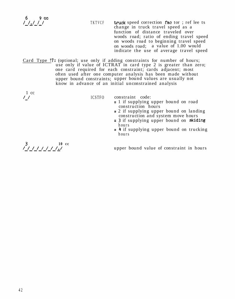
6 9 cc/ /./ / /---- T K T V C F truck speed correction fat tor ; ref lee ts

change in truck travel speed as afunction of distance traveled overwoods road; ratio of ending travel speedon woods road to beginning travel speedon woods road; a value of 1.00 wouldindicate the use of average travel speed

Card Type 17: (optional; use only if adding constraints for number of hours;use only if value of ICTRAT in card type 2 is greater than zero;one card required for each constraint; cards adjacent; mostoften used after one computer analysis has been made withoutupper bound constraints; upper bound values are usually notknow in advance of an initial unconstrained analysis

1 cc/-I

I31 / / / / / /10 cc/-,--,--A

ICSTFO constraint code:= 1 if supplying upper bound on road

construction hours= 2 if supplying upper bound on landing

construction and system move hours= 3 if supplying upper bound on skiding

hours= 4 if supplying upper bound on trucking

hours

upper bound value of constraint in hours

4 2

Appendix 6-Harvesting Example Problem Input Data

HYPOTHETICAL HARVESTING EXAMPLE: 4 METHODS4 12 2201

2 567500. 95.00 50.63 30.572. 0.70 21.6370. 14175. 0.80 lg.0590. 16675. 0.85 22.30

34.0 28.0 8.3 5.3 15.0 0.80 1800.00 lg.5034.0 26.0 8.3 5.0 15.0 0.80 2000.00 20.501 1 12 5 23 7 34 9 41 116232 1 3 42 2 1 4 2 33 13 43 2 5 93 3 9234 1 3 44 2 5 94 3 4194 4 6230

350. 15.0350. 15.0450. 15.0325. 15.0800. 15.0600. 14.0350. 15.0450. 15.0325. 15.0800. 15.0600. 14.0700. 14.0650. 13.0350. 15.0450. 15.0325. 15.0800. 15.0600. 14.0700. 14.0650. 13.0

1250. 12.01650. 12.0

1

-10.-10.-8.

-10.-10.-8.

-10.-8.

-10.-10.-8.

-10.-15.-10.-8.

-10.

-l"ai-10:-15.-12.-6.

10. 1.50 1.50 100.10. 1.50 1.50 100.15. 1.50 1.50 150.12. 1.50 1.50 100.12. 1.50 1.50 150.10. 1.50 1.50 100.10. 1.50 1.50 100.15. 1.50 1.50 150.12. 1.50 1.50 100.12. 1.50 1.50 150.10. 1.50 1.50 100.8. 1.50 1.50 150.

20. 1.50 1.50 100.10. 1.50 1.50 100.15. 1.50 1.50 150.12. 1.50 1.50 100.12. 1.50 1.50 150.10. 1.50 1.50 100.8. 1.50 1.50 150.

20. 1.50 1.50 100.15. 1.50 1.50 100.10. 1.50 1.50 100.

350. 1.5 0.3 1.00 0.0350. 0.6 0.3 1.00 0.0

2525. 1.5 0.4 0.90 2.0

4 3

350.2525. ;.i

o:g;.;0:4

;A;0.0

3875. I:OO2.01.8

6775. 1.2 0.3 0.80 2.21 1 i-1 1 21 1 41 1 51 1 '71 1 81191 1101 1111 1121 1131 114I 1181 1211 1221 1232 1 1

32 2 52 2 62 2 72 2 82 2 92 2102 2112 212

; %2 21E2 2212 2222 2233113133143 2 53 2 6

;zi

; ;1:3 3113 312

; $433 3183 3213 3223 323

65000.70000.40000.22500.90000.4000.

15000.12000.24000.16000.27000.15000.26000.

%i: l

105000:65000.

zEt*22500:12500.90000.4000.

15000.12000.24000.16000.27000.15000.26000.

3Ei*105000:65000.

zE*22500:12500.

g:::i*15000:12000.24000.16000.27000.15000.26000.

?E*105000:

26.28.16.

4;:2.

10.8.

16.

ii?15.13.15.2 .

2:23.16.

59:45.2.

10.8.

16.16.27.15.13.15.2.

2:23.16.

;:45.2.

10.8.

16.16.27.15.

:;:

3::.

485.1005.525.415.

1180.

z?285:

1095.625.990.570.520.

1095.170.900.485.820.

z:;*190:630.

z;*285:

1095.625.990.570.520.

1095.170.

I2820.525.415.190.630.

z;*285:

1095.625.990.570.520.

1095.170.900.

485.1005.525.415.

1180.

Go5:285.

1095.625.990.570.520.

1095 l

170.900.485.820.

E190:630.

F-E:285.

1095.625.990.570.520.

1095.170.900.485.820.525.415.600.630.

2255'285:

1095.625.990.570.520.

1095.170.900.

0.265.

2080.3700.1200.4000.3000.4950.4550.5050.6230.8000.5740.5050.7700.7225.

0.265.

2080.990.600.

0.1300.990.

1680.1290.1780.2670.5050.2080.1880.3660.4260.

26;:2080.990.600.

0.1300.990.790.

3000:1390.3660.790.300.

2480.2870.

1.9 5. 1.00 7.01.9 -2. 1.00 7.01.9 -3. 1.00 7.01.9 -5. 1.00 7.01.4 -10. 1.00 9.01.4 -8. 0.90 9.01.4 -10. 1.00 11.01.4 -?. 1.00 11.01.4 +5. 0.95 71.01.5 +10. 0.85 13.01.5 +lO. 0.90 13.01.5 +5. 0.90 13.01.5 +15. 0.80 9.01.7 +12. 0.90 9.0

1:; +lO. +lO. 1.00 1.00 5.0 5.01.6 5. 1.00 7.01.6 5. 1.00 7.01.6 -3. 1.00 7.01.6 10. 1.00 7.01.6 12. 1.00 7.01.6 -2. 1.00 9.01.6 -8. 1.00 9.01.6 -10. 1.00 11.01.4 -10. 1.00 11.01.4 -2. 1.00 11.01.4 5. 0.95 13.01.4 10. 0.85 13.01.9 10. 0.90 13.01.5 5. 0.90 9.01.5 15. 0.80 9.01.5 12. 1.00 5.0::; 10. 5. 1.00 1.00 7.0 5.0

1:; -3. 5. 1.00 1.00 7.0 7.0

1.6 10. 1.00 7.01.6 12. 1.00 7.01.6 -2. 1.00 9.01.6 -8. 1.00 9.01.6 -10. 1.00 11.01.7 -10. 1.00 11.01.7 -2. 1.00 11.01.7 5. 0.95 13.01.7 10. 0.85 13.01.8 10. 0.90 13.01.8 5. 0.90 9.01.8 15. 0.80 9.01.8 12. 1.00 5.01.8 10. 1.00 5.0

44

4 1 1 65000.4 1 3 57500.414 40000.

EZ 22500-12500.427 90000.4 2 8 4000.4 2 9 15000.4 310 12000.4 311 24000.4 315 6000.4 319 10000.4 416 f7xItI.4 4174 420 16000:4 4214 422 3Ec-4 423 105000:01 1 1 11 1 1 21 1 2 11 1 2 21 1 4 11 1 4 21 1 5 11 1 5 21 1 7 11 1 7 2I 181118 21 1 9 11 1 9 21 110 11 110 21 111 11 111 21 112 11 112 21 113 1

: :1::1 114 2I 118 11 118 21 121 11 121 21722 11 122 21 123 11 123 22 1 1 12 1 1 22 1 3 12 1 3 22 1 4 12 1 4 2

26.23.16.

59:45.2.

10.8.

16.6.

n5:15.8.

15.

3;:

400.460.450.

:;:-470:450.

z-.

E:420.510.550.

Et

Fig:

490:450.490.450.490.450.

go"-490:450.490.450.490,400.460.450.470.450.470.

485.820.

E190:630.

ZE-285:

1095.490.270.900.450.335.

1170.170.720.

2:450.

:::-;;i$ :

g :.

?i::420.510.550.

$2

~~:450.490.450.490.450.490.450.490.450.490.450.490.450.490.

E:450.470.450.470.

485. 0. 1.9 5. 1.00 7.0820.

600.

265.

600.630. 0.

285: zz;-1300.

2::- .

790. 990.

1095.

2080. 990.

0.,490. 300.270. 790.900. 500.450. 0.

1.6 12.

1.4

1.00

5.

7.01.6

1.00

-2.

7.0

1.00 9.0

1.9 1.6

1.6

-3. 10.

-8.

1.00 1.00

1.00

7.0 7.0

9.01.6 -10. 1.00 11.0

1:; -10. -2. 1.00 1.00 11.0 11.0

1:; -5. -5. 0.95 0.90 13.0 9.0

::; -4. -5. 0.900.90 13.0 13.0335. 2370. 1.5

1170. 200. 1.5li0. 2820. 1.5 4. 1.00 5.0720. 150. 1.5 6. 1.00 5.0

4 5

2 2 512 2 5 22 2 612 2 6 22 2 7 12 2 7 22 2 8 12 2 8 22 2 912 2 9 22 210 12 210 22 211 12 211 22 212 12 212 22 213 12 213 22 214 12 214 22 218 12 218 22 221 12 221 22 222 12 222 22 223 12 223 23 1 1 13 1 1 23 1 3 131 323 1 4 13 1 4 23 2 51

'3 ; 56 :3 2 6 23 27 1

; ; ii :3 2 8 23 2 9 13 2 9 23 310 13 310 23 311 13 311 23 312 13 312 23 313 1

; ;143 :

; ;:i :3 318 23 321 1

4 6

400.420.400.420.460.

Ek420.510.550.460.490.

Z:450.490.450.490.450.490.450.490.450.490 l

450.490.

t/g400:460.450.

E470:400.420.400.420.460.

E?420:510.550.460.490.

g::450.490.450.

400.420.400.420.460.

Eii:420.510.550.460.490.500.

E490.450.490.450.490.450.490.450.490.450.490.

:5:*400:460.450.

z;;*470:400.420.400.420.460.

E:420.510.

E:490.

2%450.490.450.490.450.490.450.490.450.

3 321 23 322 13 322 23 323 13 323 24 1 1 14 1 1 24 1 3 14 1 3 24 1 4 14 7 4 24 2 5 14 2 5 24 2 614 2 6 24 2 7 1

zx:4 2 8 24 2 9 14 2 9 24 310 14 310 24 311 14 311 24 315 14 315 24 319 14 319 24 416 14 416 24 417 14 417 24 420 14 420 24 421 14 421 24 422 14 422 24 423 14 423 21 1 0.952 1 0.952 20.903 1 0.95

; : :*g4 1 0:95

:: : ti%4 4 0:80

:120.0600.0

//

490.450.490.450.450.400.460.450.470.450.470.400.420.400.420.460.500.400.420.510.

E:*490:

%:450.490.420.470.430.460.440.480.450.490.490.520.450.

F$*510:

490.450.490.

E*400:460.450.

E470:400.420.400.420.460.

ZC:420.510.550.460.490.

2450.490.420.470.430.460.440.480.450.490.490.520.450.

E:510.

47

Appendix LHarvesting Example Problem Output Data

TITLE 14-S-T R U N = HY”OTHETICA1 H A R V E S T I N G EXACPLE: 4 HETHCOSN U U B E R O F RETHODS= 4

N U M B E R OF r)DZERS= 1NUMlER O F SKIDOERS= 2

N U M B E R O F T R U C K S = 2LP ANlrlYSIS C O D E = 0

LP CUTf’UT CODE= 0a U S E R CCNSTRAIMS= 2H A R V E S T VOLUME’= 5 6 7 5 0 0 . I N T . BOARC F E E TP R I C E I N SELLING U N I T S (St= 9 5 . 0 0H O U R L Y L A N D I N G POVE C O S T fs)= 50.t3DISTAYCE F”OM W O O D S E D G E TC FILL I%tILES)= 3 9 . 5

*,*********t********+**********DOZE’? E O Z E P D O Z E R W-NJRLY

LUMBER UP E F F I C C O S T

1 7 2 . 0 . 7 0 2 1 . 6 3

t***~**k**f*i*~***+***+t*++L*2 1 . 6 3

***+*,*******r**i************************$*********

SKI!lDERS K I D D E R SK IODER SKII?DER SKIOOER Hawit

vU*RFp WORSF~DWER WE I GHT CFFIC C O S T

: 90. 70. 16675. 14175. o.es G.80 22.30 19.05

*+*****+********+**********************************4 1 . 3 5

*++*****+****t*****+***o******************************************************** fl(lf+WOODS ** ***** yf. lQl js ****T R A V E L T R A V E L TRaVEl T R A V E L F IXFD

FM”TY LOAOEO Et4pTY LOdOE T IrlC CYCLE TRUCKTP{JCK SPEED SPEED SPEED SPEED F E R ‘IRUCY 1 RUCK HOURLY

NUHR ER N P H H=H N@H WH I . 0 4 0 E F F I C VolUnE cos 1

: 34.00 34.00 26.00 28.03 8.30 6.30 5.00 5.3lJ 15.00 15.00 o.ao 3.83 2GO0.W’ 1800.00 20.50 19.56

*****+**t****+*****************+***************************************

4 0 . 0 0

49

N U M B E R N U M B E RN E T H O O R O A O O FNVNBER SEG”ENTS L A N D I N G S

1 12 5 :3 I 34 9 4

,F,*BE9Y F T H O ! , L A N D I N G O F *4xiriJ* 4REAN U Y B F R N U W E R A R E A S C G C E hUWeER

RObC OCbCYIOTI! S L C F E

C U T FlLL aCADZLCPE SLOFE 7YFER A T 1 0 O A T J O C C D F

1 3 . c -JO. I”. I.50 1 . 5 0 lOi?.

13.0 - J O . J O . 1.30 1.30 lC3.J3.0 - 9 . J5. 1 . 3 0 1.52 130.J3.0 - J O . 1 2 . 1.50 1 . 5 0 Inn.15.0 -13. J Z . 1.30 1 . 5 0 130.1 4 . 0 -e. J O . 1.50 1.50 100.

1 5 . 0 - J O .13.3 - 3 .1s.u -10.1 5 . 0 -JU.1 4 . 0 -e.1 4 . 0 - J O .1 3 . u - 1 5 .

J O .15.

:::10.

a .20.

1.33 1 . 5 0 100.1.50 1 . 5 0 150.1.30 1.3a 1ro.1.3” 1.30 13”.I.50 1.5r) 100.1 . 5 0 1 . 3 0 150.1.50 1.50 L O O .

JS.0 - 1 0 .J3.C -e.J 5 . J -10.13.0 - 1 0 .1 4 . 0 -2.1 4 . 3 -JJ.1 3 . 0 -1s.1 2 . 0 - 1 2 .1 2 . 0 - 6 .

10.15.1 2 .1 2 .J P .

2::

:::

1 . 5 0 1.5tl 100.1.50 1 . 5 0 130.1 . 5 0 1 . 3 0 100.1.W 1 . 5 0 150.1.30 1 . 3 0 100.1.30 1 . 3 0 150.1 . 5 0 1.50 1p.1.30 1 . 5 0 lQ0.1.53 1 . 3 0 1 0 0 .

CUBIC ACFES SEGNEPlIVl“DS CLLAFFP H O U R S

46.9 0.J 1 . 94 6 . 9 0 . 1

170.177

7 . 9 173.n77.8 lOY.JU7 . 1 1 6 7 . 3 8

1 2 . 7 274.t.r1 3 . 0 2 8 6 . 2 3

7 . 97 . n7 . 7

12.71 3 . 0

1:::

1 7 0 . 0 71 6 9 . o o167.382 7 4 . 6 72 8 0 . 2 32 0 2 . 7 33 6 0 . 6 9

::I:7.1

1 2 . 71J.U

6 3 . J 0 . 3 9 . 4138.8 n . 7 16. r176.3 0.4 2 7 . 11 4 1 . 3 0 . 3 3 2 . 39 4 3 . 3 2 . 6

J70.07169.W167.382 7 4 . 6 12 8 0 . 2 32 0 2 . 7 3340.693a7.166 9 8 . 4 3

METMOO HC-lkol~H O U P S LGSl

1 . 9 170.

I2

330.450.223.R O D .600.

2 5 2 5 .

4 6 . 99 9 . 25 4 . 2

:::117

3‘

C.10.30 . 21 . 0

1 3 3 . 3rn.n

4 0 3 . 63

4 9 . 1 IOaJ.

33 ’1 . 46.9 0.19 5 . 2 0 . 25 4 . 2 (1. 1

1 3 3 . 3 G-57 0 . 0 0 . 2e3.J 0.3

138.8 0.36 2 3 . 5 1.6

J23‘

?25.3 Q O .600.7PO.,553.

7 4 7 3 .

56I

73.1 1ci3.

350.&WI.

‘0.9 0. I0 . 20 . J0 . 30 . 2

c4

__.9 9 . 23 4 . 2

1 3 3 . 3iis:300.690.703.650.

1 2 3 0 .1 4 3 0 .6 1 1 3 .

44e‘

45 70.56I3P

1444 1 3 4 . 6 ZYJO.

60

Cl SIIKCC “““I’mz Clvenrct HCUPLl CALCING 1IYflIMG S7SlfP rvstcli :::t:::airrciwwvt c

*ETwPfI LAuntNG IRlW C U T OCZEl OOZER EFFIC BUILOIYG OUILOlkG WOVErdups

COVE L WVINGNIJWEA NWRER nolJwYA~V ACRES OEPlh “F CCST C O C E CPSl halYf CDS1 HOUP s ‘““X

: I 1%. 1.q 0 . 3 II. 21 .63 1.an Z.bQ 56.27 4.P u.00 3.71 SO.272 1 YSQ. 0.6 0.3 72. 21.63 I .oo 1.04 22.51 0 . 02 2 2525. 1 . 5 (1.4 72. 21.63 O.yO 3. IF b7.13 2 . 02 2.b4 ‘90.903 1 15’1. c.15 0 . 3 72. 21.63 1.00 l.U4 22.S‘ 0 . 0 0.W3 ? 2szs. 0.8 C.4 72. 21.63 0.u 1.66 35.QO 2.Q IO‘.263 Y 3875. 1.5 0.4 72. 2 1 . 6 3 1 . 0 0 2.19 40.42 1.0 PI.13

12:

0.b c . 30.3 G.40.5 0.41.2 0.3

4.31 311.1372. 21.t3 1.00 1.04 22.51 0 . 0 0.W72. 21.6’. 0.9Q 1.bt 35.QQ 2 . 0 ‘01.2bI?. ‘1.63 I.&B l.CC 34.23 91.1372. ,?I.*? 0. P9 2.eo 54.27 1‘1.39

4.29 4Y4.62

NETtMnNlJWRF~

:

:

:

:1

:

:1

:

:

:

:

:

:2

:

:

:

:3

:

:3

:3

:

:33444444444444444444

lANolNGWmfP

t

:

:I

:

:I

:I

:

:2

:2

:22221

:7

:

:

f

:

:33I31

:1

:?222233114I.4444

PRE APUnaEC

I2457s9

I**

::

::

::

::

:45b7

i

:t12

::1821.? :a3

:‘561I

1:II1213

::212?23

1345

;9

1::1‘

:;

::202 ‘2323

ACEAvl?Lu*E

bSQ10.70000.4wno.22500.9ooon.

4000.1 SO00 .IPQOO.24noa.1aono.21CGO.1 sooo.ztloon.3GQGG.

LOCO.105nn0.

CSOQO.57500.40030.ZZYW.‘2SOQ.WOOF.

4000.15000.12000.24000.IbCW.270~10.15000.26009.wnoo.

4QQO.lQ!iO7Q.

b$QOi’.57!!00.4OOr)G.?ZYw.12’00.WCJO.4GW.

1 sow.12EW.24C00.16000.27Qnn.1 SW?.26039.?CFOO.

bOOtI,‘OWW.65000.~75’)O.40030.22son.12500.WOQG.4000.

15080.12000.24000.

bO9Q.lGO’)O.37oon.15000.1bOCO.3ccon.6000.

10s000.

AREAACPES

2t.20.le.9 .

45.

1::e .

le.

:‘;:IS.Ii.‘5.

3 : :

:::It.9 .3.

45.

1::

1::

:::IS.13.IS.

3 ; :

:::lb .5.Y.

45.

1;:

2".lb .27.‘3.13.IS.

2 .33.zt.33.it.

5 .5 .

43.

,r:

1::t .5.

31.IS.a.

‘ 5 .2.

3s.

*INIKC* MAXIPWSKICCING SKICOINGUISTAYCE OISTAhCE

415.WJS.

s25.415.

IIRO.275.F4Q .285.

109s.625.590.575.520.

1095.110.9-m.4e5.C20.52s.41s .‘90.630.PTS.445.267s.

1095.621.990.570.520.

IGaS.‘70.900.495.czo.525.415.190.t30.27S.445.235.

1095.tzs.WV.L70.520.

‘095.l7C.Ma.4ns.etrl.52S.415.190.b30.275.445.205.

1095.49G.no.WV.450.335.

1170.170.120.

4CI.1005.S2S.415.

Itan.27s .840.2e5.

1095.425.990.5-m.‘120.

1095.‘IO.900.4er.820.52s.43s.‘90.630.275.445.2Q¶.

1095.625.9vn.57G.SZG.

1095.‘76.900.405,820.52s.4‘5.690.630.21s .449.2cs.

1095.625.SW.570.520.

1099.170.ecn .4e5.920.s24.415.MO.alo.2Y5.441.265.

109s.49G.270.306.450.

Go’:17n.720.

FlXfOSKICOINGDISTANCE

0 .2t5.

2oQG.3710.LOW.4000.3Qh).49SG.4550.snso.t.230.aooo.5740.soso.7700.7225.

0 .205.

2oQQ.990.LOO.

1 3 0 : :

1X”,:1290.1710.2670.5nSQ.ZllPO.11100.364G.4260.

:I.2t5.

20110.990.(100.

1 w::990.740.

n.300.

139n.3tbO.

79fi.JW .

24PO.iQW.

0.2t5.

2 c t o .9 9 0 .bon.

130::

2:n.

3 0 0 .7 9 0 .Yrn.

2 3 7 : :2lw.

2?20.

SKIOOlNG WAIL SLlm!COPPEClICN ItlAViL Liiikij

f AC IUR OlREcrlcY 111.

5 .

1.90::21 . 4 01.w1.4aI.401.501.501.501.h)1.701.701.70l&OI.60l&Q

::2‘.bO1.w

::23.401.4*

::,”1.w1.5Q1 . 5 0

::,”1.WI.90

::!z1.66I.40

::21.701.71I .70‘.biI1.m1.00l.RO1.801 . 9 01 . 9 01.90l.bO1.60‘.bOl.QU

::zI.70l.fO1.701.50I.501.501.501.501.w

- 2 .- 3 .- 5 .

-16.-*.

-10.- 2 .I.

lb.10.5.

:::

:::3.5 .

-3.‘ 0 .12.- 2 .

-6.-10.-2.

Y.:b’:1::6:5.5.

- 3 .

:;:- 2 .-I).

-10.-10.

-2.

1::IU.

5.‘ 5 .12.‘0.I.5 .

- 3 .IO.‘ 2 .- 2 .-d.

-10.-IO.

- 2 .-5.-5.- 4 .-3.

3.4 .46b .

APCA fIXLOOIFC ICUL?V 1 WE

FAClCl E1bf.t

1 . 0 01.00 :::1 . 0 0 141 . 0 0 1 . 5

Ii:2 :::1.00 IArc)1.00 IA.00.90 rl.il0.80 13.e0.90 13.30.w I3.Y

o.ao0.90 2,”

PC . :*:

::ii1:o

1.00 2:1.w 1 . 01 . 0 01 . 0 0 ::I:

:*z . I:::

::c‘ 1 . 0IA.0

0.90 11.00. co I,.00.w l3.Ga.vo 0.3o.eo ~.o1.001.00 ::t

1.001.00 :-:1.00 r:c,

1.00:::

:*:9:*

::: 9.QII.0

I.00 l1.dI . o o I&.*6.50 l1.UO.CP Il.00 . 9 0 13.0n.90o . e o :::1 . 3 0 5 . bl.CG 5.0

‘*ao i-8l.W::iZ 110

1.00 :::1 . 0 0 9 . Q1 . 0 0 9.J1.00 11.0

::z1A.JAI.0

0.90 13.00.90 9.9o.on lY.OU.90 L1.Jbe0 9.~

61

62

11

:224‘455q?77

ms3991

1J

:‘j

::1‘12‘ 212131313‘4‘ 414141Rlr)21

::22

::23

::

12

12

12

12

12

12

12

12

:

17

12

:

:

12

12

12

nlrlMurVOLUHE

SK IDOFD

4’)o.n463.0

45fl.0470.0

45n.047C.O

*sn.n470.11

46”.05na.r

coo .o420.0

510.F550.n

4 6 0 . 049O.P

500.092F.P

450.049P.O

450.0490.0

450.0490.0

450.049o.c

450.0490.0

450.0490.0

450.0490.n

1141 IMU’1 CYCLE NIJMSEQVCLUPE T‘NE O F

SK‘OJEO NIhUTES CYCLES

400 .J ‘9.914 6 0 . 5 lC.51

450.2 ?2.45470.0 27.21

450 .J 42.8‘470.0 35.43

4 5 0 . 5 5P.7‘470.0 47.F7

460.3 40.C55OU.J 33.4’)

41X.3 .J 64.2‘420.0 62.82

510.J 57.Nf5Q.O 47.7‘

4 6 0 . 0 76.40490.5 62.58

5 0 0 . 0 102.74520.0 e4.3tl

4 5 0 . C 121.8R490.0 ‘61 .Cb

450.0 1 3 6 . 6 9490.0 112.57

4 5 0 . 0 148 .72490.0 121.35

450.0 131.5649O.J 10.5.37

4 5 0 . 0 120.2fl490.0 98.73

450.0 117.11490.0 95.19

450.0 Iza.61490.0 104.40

‘63.141.

‘56.‘49.

09.95.

50.4a.

196.110.

‘0.14.

2c.27.

2 6 .24.

48.4c.

? b .33.

60.55.

?3.31.

5R.53.

6 7 .Cl.

13.‘2 .

233.214.

dREASKI0IiME

ncdJRS

51.2138.89

e4.136 7 . 5 4

63.4250.25

48.933e.27

130.54‘00.4H

10.708.38

28.2321.69

33.2525.7‘

a2.1964.9‘

72.2355.00

136.69‘03.38

8 2 . 3 461.91

126.6955.84

‘33.56100.75

26.0319.43

500.16372.85

AREA LANDING LANOING rEwa0 rre1noliSK‘COIRG SKlfl01hG iK 1UOlt.G

kaws nouas C‘JSTS

2 2 . 1 0

37.46

28.04

21.47

56.79

4.10

12.27

‘4.50

36.27

31.22

cE!.ec

33.34

!4.56

57.43

‘1.12

213.616 9 5 . 7 5 2 0 7 6 9 . 1 3

6 9 5 . 7 5 287S9.13

(lETRonw

2

:2

:2

:2

:

:22

:

:22

:

:

:22

:2222

:222

:

:

:2

:

:

:

33

L 4wYO

t11

:

:11

:22722

:2

:2

:2

:

:2

:22

:2

:2

:2

:

:2

:

:

11

AREANP

:13

:444

555646777

8”a9

i10

:!i11

::

if1213

::1414

::19

:‘:

::

::22

::23

11

SK10Ml

1

12

12

12

12

12

:

:

12

:

12

12

:

12

b2

12

:

:

M‘MIUUN CLX ‘Mu* CYCLE NUWWIVOLUME VOl.U*E TIME O F

S K IDOFO SKl0OE0 HlhUTES cYclES

A R E ASK10Tl ME

HOURS

400.0VJO.0

450.0470.0

45n.n470.0

400.0 17.194 6 0 . 3 15.12

450 .o 27.N)470.0 22.Sb

163.141.

‘28.‘22.

44.5735.62

57.4946. R2

450.3470.0

40.5333.53

CO.bS4a.13

400.0 400 .o 28.95420.0 420.0 24.t2

.9’;.

5 6 .54.

27.1421.99

400.0 400.0 19.55 3 ‘ . 10.18420.0 420.0 ‘7.05 30. P.46

460.0 4elI.0 21.t1 1 9 6 . 70.475 0 0 . 0 500.0 18.94 180. 56.a2

400.0 4oo.a 21.39 10. 4.73420.0 420.11 24.26 10. 3.n5

5‘0.0550.0

46O.ll490.0

3oo.n520.0

5 1 0 . 5 30.36 29. 14.88550.1 2 6 . 1 7 27. 11.89

4bE.O 34.21490.0 29.22

2 6 .24.

48.4t.

‘[email protected]

500.0520.0

450.6490.0

45.4.138.22

3 6 . 3 229.4D

450.0490.0

450.0490.0

450.0490.0

53.5845.66 :;:

60.55.

33.31.

58.53.

67.61.

:::

233.233.

31.7524.a5

450.0 c7.09490.0 73.10

450.0 IlD.lfl490.0 91.73

450.0 50.99490.0 42.el

450.0 74.tb490.0 62.47

450.0 5e.a?490.0 48.47

450.0 82.00450.0 66.70

8 7 . 0 96 7 . 1 4

t1.5n46.60

450.0490.0

450.04 9 n . o

450.0490.0

450.0450.0

49.1037.36

8 2 . 9 6t 3 . 7 4

13.079.89

318.99259.37

wo.04 b 0 . 0

wo.0 le.91460.0 16.51

163.141.

51.2138.09

AREA LANDING LANDING MEW00 nt 1 t,coSKIOOlNG

lfaURSSKlC”W(;, SKIOD‘NG SKlOOlhG SKlUlJl*G

CGSTS nouns LIJSTS

20.18

25.80

26.8372.02 3011.06

‘2.15

4.62

31.46

2.12

6.61

t.62

‘6.25

‘3.94

37.91

2 6 . 5 8

i l .37

3t.05

5 . 6 3

‘43.03364.33 15065.10

437.15 18076 . l b

:

I2

:

1,

I*

1I

:

12

t2

I2

I2

:

:

:

:

:

:

I

‘ I O . 0470.0

30 .0 .P5.“

179.122.

‘50.0‘W.0

52.9135.43

89.05.

63.32%I.25

‘OP.0 ‘t%l.O 71.55 16. 27.1242F.F ‘20.0 ZI.C2 s.. i l . . .

.nn.n420 .0

40u.0‘ 2 0 . 0

2?.E.l...h

3‘.30.

‘2.P)9 .90

660.0‘ 1 0 0 . 0

‘ 4 0 . 0soa.

?I.(11C.G‘

L.C.1.3.

WO.0‘ 1 3 . 0

‘W.0.,!,.n

29.2924 .26 :II:

4.733.M

lO.?b26.11

75.7T.

tc.de“.*.

4W.J‘ 9 0 . 0

‘60 .o5VO.3

25.El?2.%

26.2‘.

II.229.2,

3gn.o 503.5 I? .5’* .e. 27 .1 .520.” ,Z”.O 2 9 . 1 ‘ ‘6. 22 .3 .

‘ S O . 0 ‘5O.J 35.33 ?b. 2O.W‘9V.b ‘W.J Il.02 33. Lb.19

‘ T O . 0 ‘51 .0 69.8. 60.5 9 0 . 0 ‘90 .0 59.23 $5.

‘ 9 0 . 0‘PO.@

4QY.n‘.O.il

‘SO.0‘90.0

‘50 .0‘50 .0

‘SO.0‘50.0

‘50 .0‘90 .V

‘SO.0‘5P.O

“1.391 3 . 0 ‘

34.e.25.83

81.II.

50.13.

‘ S O . 0‘.O,(’

‘ 5 0 . 0r.lf.0

‘50.0‘9O.F

Sl.9. 67 .‘4 .03 61.

+2.11 13.33.57 ‘2.

65.15 233.53.79 233.

65.0356.39

5’e.ss37.2s

33.5526.39

51.6‘‘4 .93

9 .4 .7 .2 .

‘00 .0 ‘00 .0 Il..1‘60.0 ‘ 6 0 . 0 lb.¶l

‘50 .0 ‘50 .0 30 .01

163.‘41.

128.

21*+0020 . . ‘(1

S1.2‘39.99

b..OI

C‘K l”“”VCLUME

SXI‘WEV

- -mtt LINU‘NG L‘NVING MEW00 MlI~CO

sK1*o,hG sxloolht JKIWlhGwu*s WULS ‘“SIS

22.13

79.C6

2ll.OC

ii.15

5.43

?,.‘b

2.,2

C.6‘

l .a

12.27

0.39

30.511

2l.OI)

L4.77

25.2s

4.11

llY.13

22.10

5

1t.90 3259.22

51.11 23ee.b‘

237.59 5b24..937‘. lb 15‘71.31

“EIYO” LWONa

.4‘‘.‘‘4...‘44‘4.‘..‘.44.4.‘..4‘.‘‘4.‘.‘

:..‘..‘4.4...I(

N O

:I1

:

:2

:7

:2

:22

:23

:13

:

:3

:3‘4.....5..‘.4‘.44..

2

:

:

12

:

:

:

:

:

:

I,

:

12

12

I2

:

:

LUIVING L4NOlNG NEW00 rKlWS”W~IW4~ SK‘OOING SKlOOlhC S~lUOlhG

cosrs H O U R S COSIS

‘70.0

‘10.041a.o

570.0 5l.bb29 .bb

‘50.247O.J

25.w

4 2 . 9 ‘?S.O

‘22.

Y..11. 2::.

27.1+21 .9 .

2 8 . 0 .79 .90 32S0.22

:9t*6

:1e999”9

‘00 .042n.o

‘00 .0‘20 .0

211.5’124.t2

36.3‘.

‘00 .0 ‘UO .o .23.0.*LO.0 420 .0 lP..b :::

12.039.90

12.1s

5.43‘60.0 ‘60.0 2l.Cl 1 9 6 . 70.51500.0 YPP.0 1e.r. 180. ‘16. 82

.00.*‘20.0

‘00 .O4W.b

5‘9.0550 .0

5lO.dS50.U

;p;:.

30.3626 .17

LO.1 0 .

29.27.

4.733. e3

31.a

2.1214.81‘1.J.

h.6157 .77 23dO.61

‘9‘0‘9‘1

::1sIS

::

::

‘40.0 ‘C0.U 2l.b‘699.0 S90.0 22.36

11.229.21

5.065OO.Js20.0

5PO.O?Zd.J

3 3 . 9 .29.11

2 1 . ‘I22 .3 .

12.27‘5O.E‘90.0

‘50 .3‘90 .0

30.6121.0’1

t . e o1.53

3.05‘20 .0 420.5 26.30l 7a.n 670.0 22 .93

L O . 4 7e.13

4.91125.9s ‘031 .06

I*3 6lb17‘1

::20

::

::

:t2;

::23

‘30 .” ‘35.0 39.96460.0 ‘60 .0 34.23

56.7‘‘5.89

25.37‘W.0‘0O.P

‘SO.0‘90.0

590.0n20.0

‘50 .0100 .0

l 70.0110 .0

“ 0 .a‘10 .0

455 .0‘90 .0

‘90 .0(20.0

450 .0$00 .o

470 .05‘0 .0

21 .2322 .17

w-55‘1.4‘

42.63lb.26

‘3.2635.1+

20 .5217.31

:::

‘8.‘(1.

13.‘2.

:::

2

3 ‘ .3‘.

36 .33.

61 .31.

:::

!23.206.

‘4.33‘I.96

33.5125.82

‘?.3034.06

9.6‘1. “I

7 6 . 0 459.6‘

6..9

‘4.59

‘9 .35

4.10

33.411 0 3 . 3 1 4 2 1 1 . 9 9

2*4..3 lO950.56

. . ..*...*..“*~.**...~......*.*....*..*....................*..~.....“...........~“*.*.*...*..**.*.......~........I****..

PVEPAGELANDlNG L 4NO ING LANOING HE 7hUO HETHOO SKIllDING

YUf4RfR VOL WE PCRE5 VCLWE AC&ES i?lSrANCE

I ?f.,5n?. 493. 686.5clSCP. 283.

1 162~lm. 6 5 . [email protected] 4J”‘iYl~,. ZIP. 586.

5675AC. 2R3.I 1t..,50’1. 63. Lllh2 1+40P!l. 4 3 2 .3 2tlOo~l.

,2::tv4.

C-61500. 2a3.

P E P LANCITC

AVEP AGfFIXED

SKICDlhCP I STAVCF

‘ 2 9 6 .

732.201t.

YEIGHlFOAVf94GF

lR4VELSKIGOINGCISIANCE

bhll.

15P7.3212.

782. 1111.1 1 6 . 1221.

13sr. 3 2 0 4 .

. . . ..I...OEK ‘IE,H(JO .A... . . . .

bfIG~lL5AVEK AGE AVYkAirt

AVERAGE FIAEO l*aVtLSKICUING SKlCCfhC SKlUJl*U01 STANCE OISl4NCE CIIIANLE

b f b . b29b. 4 8 7 1 .

554. 1 3 9 9 . LIAI.

5 7 9 . 985. i!Mt.6 I 102500. 65. 61th 722. 1771.I 1hCOJ. I l . 432. I?#. l221.c

35zaar. 35. 5 3 5 . 4 7 0 . 1524.

4 6 2O9403. 112. CZL. 1 0 5 7 . lSR3.‘ 5bi100. 2 9 3 . 5 5 0 . ?5P. 1 5 4 0 .

. ..~.~..*.*...*..~.**.~*~*.*.*..*.~.*..~..~~~~~..~.*.****~...*.~*.**~.~*.~*...,..*..**.*~.*.~*.**~***..*.**.....*.*,**,*.*~~~

*.,**..*.** . . . . . . . . ********1IlIlCY

rP4veL;ynQ; L:$;;; COsctCTION

F A C T O R

: :‘1.990.9s

2 2 0.w3 I 0 . 9 5: : u.90

0 . 9 54 1 0.85. 2 0 . 9 0A 3 0.15A A 0. dP

.**.****..***..*~..*...*.*.

M E T H O D LANOlNG TRt.JC KNUMBER NIJJ’BER NIJWBEP

:11

2

52222

3333

333134444444444444

:1

1

:

:

I2

:

12

1 2 . 9 9 80.0 2 3 9 . 2 02 3 . 1 0 7 2 . 0 2 2 3 . 3 3

CYCLE NUMbERTINE O f

WQURS CCJAOS

2.e22 . 9 3

215.32 e 3 . 8

TRUCKTIME

HIURS

889.62830.C5

2 . 8 2 9 0 . 3 2 5 4 . 7 42 . 9 3 t 1 . 3 2 3 7 . 8 5

2 . 9 5 2 2 5 . 5 b72 .743 . 1 0 2 0 2 . 5 626.12

I.82 eo.3 2 5 4 . 1 42 . 9 3 61.3 237.E5

2 . 9 9 3 0 . 0 2 3 9 . 2 0?. 10 1 2 . 0 2 2 3 . 3 3

3 . 1 03 . 2 2

1 4 5 . 01 3 0 . 5

4 4 9 -804 19.s5

2 . 8 2 9 0 . 3 2’14.742 . 9 3 81.3 2 3 7 . 8 5

3 . 1 0 2 8 . 9 a9.t13 . 2 2 26.0 03.ir7

3 . 3 5 116.1 3 6 8 . 5 53 . 4 7 1 0 4 . 5 3 6 2 . 7 5

**++* A L L T R U C K S WOPKINC T O G E T H E R I)++**LANOINC LAN0 INC METHOD

T R U C K I N G TRIJCKING TRUCKINGwJns COST HOURi

METbIOOTRUCKING

COST

4 2 9 . 5 6 1 7 1 8 2 . 4 84 2 9 . 5 6 1 7 1 8 2 . 4 8

1 2 3 . 0 0 4 5 2 0 . 1 3

324.e3 1 2 9 9 3 . 3 0447.e3 17913.40

1 2 3 . 0 0 4 9 2 0 . 1 0

115.50 4619.34

217.18 8687.214 5 5 . 6 8 18227. lb

1 2 3 . 0 0 4 9 2 0 . 1 0

115.50 4619.04

43.21 1730.79

lE7.60 7504.204 6 9 . 3 7 1 8 7 7 4 . 9 1

LI*******+**~+***oo**

CONSlR4INlCOOE

I- RO40 HR29 L4NO M\ UPPER39 SKI0 HR BOUNO4= T R U K Ho VALUE

1 120.3 600.

64

PFTWCD sl,l*PPY.*..t*l**..t**.*.***..~~*~*.*.*~*.~~***~*~..~*.~.*******~*~*~*~**~*~*...*~*~.*~~~*~.*******.****~*,~**..~.~~**~..*********..**~

La*4DIVi CCNSTRLC110N TCT.lL N6THUJRrJ4” COPISlRuCTIOh( AN” !YllEH 90\, IhC SKICCINC TRbCKILG ,tET*CJ ~~RVflIlllt

NET,, ______--_-------.--- - - - - - - - - - - - - - - - - - - - -em----me-- -_--- - - - _------_-_------___ nlE”tSTIr,G UNITN J H O U R S fll f /V(rL H C I J F 5 04 IIVCl muds IS3 TIVCL bCUPS 1,s ,,"CL CCSTS COSTa

1 9. 170. 0. 1. 56. (1. 6F6. 20169. 51. 430. 17137. 35 . 4 6 1 7 7 . 9 5 6i.ji2 49. 1061. 2. 3. 101. 0. 431. 1eo7t.. 32. 448. L7913. 32. 37241.81 BS.623 15. 1625. 3. 4. 311. I. ,74. 15471. 27. 456. 18227. 22. ?563S. 38 0.. 194 135. 2~10. 5. 6. 45’. I. 265. ICSII. 14‘. 465. lb775. 33. 33lwc.44 id.31

*~***.*******t*******.**~*.******~**~.**.~**~*~~~**.*.~**.~*~*.**~*~**.*~.**~.~***.*~*.*.***~**~***,~*****~*****.***~**...*.~*

IlFRATl~N WI- 1

.~.~*.**.***.**.**.*.~~~*..*.***~~**~**.**,.~**.~**~~***~.~****.~*.**.~**..*.******~=**~****~***.*~*~*.**~***~.~***.***,****~.*~

l . . . t *l . l CJ * 95.JJ -;I.t? -72..?e -41. f 5 -4P.Od I RlLhI -l tg. . . .. .a* ~.*~*~rt**+*t..****~~*~*~~.,~**~~**,~~***~~*~~~~~~~*~~*~*****~*.**.******~**..****..**~.*.***~.****** mnu *

l *s* l SElLI�,G * PETHCO * * E ? H G O * “ETb*O . nETno l . IlHR * %,rR * I/W l ,IHR * l

. CB l I* * PRICE 5 l 1 * 2 1 2 * 4 * * CCIO, l L4hC t SKiL * TWCK * Ccnrlnhrs *

l t s+ l cm, l lr-1) l 122) . (M3l * lF4i * t 1211 * IL21 * 1131 * li4, l t

..*..**~*.*~,**~***t.*.~*~~*~*~..~*.~~*.~**.~~~*..~,~~***~*~**.***.**~*.**.~..*.~.~***~*******.*.~*.**.*.*~****~*~***~******.***

. l l

+ **.I-n l ⌧,0* 1.w - 5 6 7 . 5 0 -561.50 - 5 6 7 . 5 0 - 5 6 7 . 5 0 n .@O U .OiJ 0 .no MO:l

i.au *I n.7o l rll* 0.00 7.86 4 9 . 0 1 7 5 . 1 2 134.55 - 1 . 0 3 0 . 0 0 0 .JO 0.00* 0.☺.☺ *

* 0.00 l ⌧12* 9.30 0.70 i.t4 4.31 6 . 2 5 0.00 - 1 .,h, n.oo 4.00* 0 . 6 0 ** o.‘),, * ‘(13. 0 .UF 655.,5 437.15 374.16 264.F3 0 . 0 0 0.w -1.nu U .n0* 5.03 *l n.oo * ⌧14* *.on 4 2 9 . 5 5 447-E: 455.bR 469.37 0.m 0.00 0 . 0 0 -,.oo* O.OJ *. -21.03 * x15* 1.W O.CO 0.00 a .w ll.J” *.,w 0.w 0 .I30 P.JO* 541.50 l

l - 7 2 . 2 6 * X16’ O.OQ 1.00 i -00 1.m l.GJ 0.03 0.6%) 0 .o�) 0.00” i.03 .l -41.35 l XL?+ 0.00 0.00 0.00 J .u3 J .JO 1.03 @.OO 0.30 *.dl** LZlJ.DLl lc -4o.cfj l X18� o.up 0.00 o.ao ~~.OO c.w C.�il 0.00 I .t+o O.GQ� ti*cl.w *

. l l t I

*.*~..**.**t.t**t**f****~~**~****~~~..***.****.~**.*********~*******~~.**~****~*.~***.***.~**.*******~*.**.**..***********.*.*.~

l . * 7; *l c-am PCW : 35.50 r).ilJ O.CG 0.00 a.co -21.t3 -72.20 - 4 1 . 3 5 -40.03* I).*ttt.t***t****...*~..***..**..****.*.**.*.~**~.~.~*.*.*~~****~**~****~**.~~~***~*************..~~~*.*..**..**.*.*.*.**~**....*..*

bFTEe 1E IIEPbTlCNS 7 1 - f OPllWJP SCLulICN CCLSISTEC O F :~..*.*.~**.t.**.~t~****..*.*.*~~***..**~~.~~,~,,.*~*.~~~.**~.~~~...****~***..*~~*******..*..*.****.****************.****..**..~*

1040 9OSO LAhCIhG C C h S T L A k C l h G C C N S T T U T A LPF W O O w7niltu C O Q S T C C N S T A K C SYSTEP & N D IYSTEY SX1001hG Sh IDOIhC IPUCK ING TRUCKIhG M E T N O D

I PRrlPOC7 1 0 ~ ~ H O U R S C O S T S C O U P 5 C O S T S H O U P 5 C O S T S H O U R S C O S T S C(rST 5

___--- ---m-v

OIFFEPEYCE: ,A)-,#,: zu199. 3 5 . 5 9*,“..~..L.**..*.*..*t*..~*.*.****t.C**.*L*,,~,*~~~l.***~*.l**t*~~***.~.*..******..~~~*.*.

_ _ _ _. 0.4~ l Y e* -0 .co - 1 9 7 . 0 9 -15.05 O.OU -0.00 -O.DO -0.00 I .oo -o.o*+ L91.59 *l 0.9� * ⌧ v* -il.on LO.62 1-a* 0.00 -0 .co -0.00 -0.00 -0.00 I.009 ‘.bb.J.? sl -4J.JQ * x19* [email protected]?0 197.83 15.08 4.0” -4.00 -4.ou -0.00 -0.00 -u.oil* 30b.M *l 0.00 l ‘( 5. -* .w -1.13 -0.44 b .00 1 .co -3.00 - O . J O -0.k.30 -o.ao* 0 . 7 6 +. 0.00 l ⌧ l * 0.03 2 .1 3 1.44 1.00 0 .oo 0.00 0.00 0.00 o.oo* Il.24 *

* -72.26 l X16. [email protected] - 0. F 0 a.00 o.nn -n.nn -0.00 -n .oo -0.00 -O.UO* 0.40 l

l n.oc l ⌧ 6� -@ .03 0.00 -0 .oo 0.00 -0.00 1.00 -0.03 - 0 . 3 0 -o-00* 113.05 *

l l l . l

.~~.~..*~~~*~.~~~~~~..~~~=~~~~~~~.~~~~~*~~~~.~.~~*.~~~~*~.~~~~~~~~*.*~~~.~.~~.~~~~~~~~.~~~~.**~~~*~~~~~*.~.*~~~**~*~~~.~*~~**.~~

. * * 7=

, c-e** WY * 3.03 -76615.56 -49i.fe 1.00 ;I.co 0 . 00 0.00 0.00 0.091 .wm.=*~..*~.....*.~**~.*l*..***.*.**..*~~.*.**...~.*****~.~*.*****.*.*~..*.*..***..*.*~******..*.***.*.********.*****..**.~.~**~***.*.********.**** *.* L****LL.C***..,*****t***.**. l .* l t**LCL.*.*L

l . * * . * * * . . * * . * * * #HOVE V A L U E S I N C - B A Y C O Y l .* A80VE V A L U E S I N C - 8 4 R R O W l * * * * * . * . * * *

**�**L******.*. A R E DEhALTY CCSTS ..* APE Snlook PRlCES ****.*.**.**,******L*.**t**l I** **.****.*..*.****.***.***..* **. **********.*,**~t*~*.*****.~.*..*.~*******~*~~***~~~*~~.*.~.***~~.**.**...*.~*.*..~***.*...~~***.*~.***~**...~****.*************.*****~****~

SENSilIV!TV ANdLYSIS

USEXS FAMILIAR WlTH C? SHOULC BAKE C#AhGES IkINPUT COSTS ICJI PXD DESOUaCE LIMITS te.,, TOrECOWE Ea"IL149 WITH Tt‘F SENSITIVIII AhALYSlS AS I,APPLIES 70 THE CONVEY-ISCCUAhl-~EldGn FCQP~LPTIOYCSFI ,*I L-0-S-T

PENALTY COSTS AQC CH4U;E IN OUJECTIVE FUhlClICh VALUE FER VCITINCREA5F lhl NO+DPSIC VARIAb165.

IO -67.94711 -t*.42t1 2 -72.26013 -41.35014 -4a.cca15 -27.05317 - 4 2 . 7 5 6

2 - 7 6 6 9 . 5 6 33 -492.084

P”d SHACOYNUNSER PRICES

a.000a.ccaa.coo0.0000 .noo0.000a.0000.0000.000

R A N G E S R N NO’,-BISIC CIJI

"9914RLF LOWFF L,WIT

10 b7.541il1213

::I?

b4.42672.2eDk1.3Sl-l40.50027,05342,7Sh

2 lhC5.5633 492.8rz4

RbNGES c-N A&SIC CIJI

VdRllBLE 1WFF LIMIT

1 6 -38559.d50I!? -22.2&l

1 67.54,4 - 3 4 i . b r . 45 -2543.590

-64.425 ,L737?.P*.O-hQ3.4?5 Q.POO-71.Y32 -13.3fl?-74.dtI ~.O!-l~I

RANGES ON t)tIl

,

50?.500'74.124

-559999.000504.219

-99s999.300-a.c.on

I .OIlD274.,24504.ZlY

Is352.7op30 . 5 4 6

9~C79~.llO4

2543.5901124.I23

66

Appendix 8-L-0-S-T Program Listing

L-o-S-T IS DIVIED INlU2 ICTIWS; lIEFIRST§CTIOHC4mAlESLDGGIffimPH)MsmnCTrwussTESEOE~SASIKWFCRMLI~PRWW

_._._ __.. --_-. .~ ~.W.R?=QMRSIUdFKU4tl5ICFEETTOBWWFBT

nEsE cxNmsIcN5 #IE QCY !Bo IN xIIDIffi n& Epr\TI(M

WWR.7O~ (AnllE(IIR),ITR=1,16)07200 7OFUWT(lW)073%' YIX~KW.KJ) (ATIlLE(IlW,IMl,l6)07403 81 FW%T(H~~/.M.'TI~LE L-U-S-T w)1='.4X,16W07503 Gu

Ez1lX,‘LIlZERS=‘,2X,13./,2X,‘~ CT %IIZB=‘,2X,I3,/,24X,%.MER ff TMU='.2X.I3)

fi%HW’EW 125WpN9,LFW ICTWT

crml125 FCMTt4; ‘u, AIy\LtSIS f.&=’ 3X 12 / 6X ‘LP OVWT a=‘,

13X,I2,/,2;,‘# USER mMIw\IHTs=‘:3X:Ii) *mm bbIClRATt5_ _ _ __ __ . . .

ii%

t@tWIWICIPAT+lO

cQ7wcx zE3oalrKiEAul.LtEiwAY

%K

if%03 I50 Iimw1.mw 140 IzAK=l,B

Eial 133 Ii!AW1,25REAVwAw,IzAK.IzAVAb0.o

lo4al l3=lo%TIME1m 14oaxTIME1o6oo.lBCMIHE107al cx108oow(uJ9wc.xll0mC.K ZOMairZELECEDiWAKLEDINLPSECITO(ffLOSllllca w(1l.m ill 170 ILul~1.2511Jx) Ill 160 ILs?-1;25114al A(Ia22,ICUlbO.o11503 160 axrIMEllml 170 OxTIMEllxa a, ls 12om=1,1111830 m I83 mJT2d.mllwo LoxT(Izam,IzalT2bo.ol2u.B lfBaINTIKE12100 lB5o.xTIM

E03 190 mrr3-1.25cI(ImJI3mo.~-

%CtIZM3&O.OP(IZCUT3bO.O

I2603 crpcIzaJT3)~.ozJtizaJT3,40Ivm(Izan3)d).oKosTuzar3)~.0w(Izm3)=0.0af1zon3bo.oaM12am3bo.0OP(IZCUT3bO.Oao(Izanwi.0W I Z C W 3 b Q . Oao~UaJr3,~.0B(IZClJT3bO.O

203 F1RM(T(II.1X,FlO.0.1X.F7.2,1X,F7.2,lX,F5.1)IFWNIT.EQ.l)I#UTE(kW,250)tWNr

25DFOMT~2X.‘HRWST WArrrW='@DWNIT.EQ.2)I

33 FoI(Fy\T(ZX,'tbW

fit%

3% FCIWTt2X ‘WMST WriW ZtX Fll.O,Zx,‘~IC FEY)IF(IWIT.kJ 4)tRIIEW 3E&Wi

16100360 FlRWT(2X YiWiT Kl.k=' 22X,Fil.O,2X,'~',

Km(KIJ.~m)m.s~,h162m 400 FcRFy\T(PX.'FRIE IN SU.116 tMl5 W='.l5X.P8.2./.2~.

1693 m-475 IdlB=l.Nm17ozsl IF~ILNIT.EO.lKOMET~l,IR~~~~.Oin03 B(I~IT.EP.P)UXFET(l,Ia00)L)(sRW1000.017200 B~Iu(IT.EQ.3~uMI~1,I~~)~~.O17x0 ff~I~HIT.EQ.4~~~1,t~oo~LHaR~1.o17400 47?imTxt4.E1750l 95ZtC=O.O

6’7

17cIll m 6x1 1a01=1,wR177WW178COw(17933w(-MpE4 -

EE18203 lx DZIIpH()=mzB HRSEFWR; 0ziw0=axol EFFIcEIMx183x W C DZlw,=mZER tKw.LY OMT; 3@x=SDlzEx184arx taRlYcosTl8mwc

ik%REm(KR so)Dwp(Iaol) aP5(IaOl),(;mMffIaOl)

5co FoF3RTti4 0 1X F4 2 1X Fi 2)163l.l 94mx&i&&inioii18900 ~IT(KW,SM))Iam,cmbP(iuO1,,~(IaO1),~(~~01)1Wll 550 FClWT(QX,I3,2X,F5.0,3X,F5.2,2X,F7.2)19103 605 awIME192cn bwTE(I(W,650)91DM:19303 650 F~T(/,W.29(‘*‘)./,23X,F8.2)194Ol WIlEWl,7CO)19500 703 F~l~2~/~.2X,51~‘*‘~,/.46X.‘sKI~‘.~,

:F%12x,'9(ImER'.6x,'sKIoDER',3x,'sI(IocER',2X,2'SKI~R'.6X,'HM(LY'./.3X,'KM3ER1,3X,

19m ~'HRSEFDIER'.~X,'YI(;HT',~X,'~IC',~,'~KT~,/)

uwE(w,900)9aKH:900 FCIMTU 2X R('*') /

mwW:95i)) "45X,F8.2)

950 FClUMPU) W 78('*')/,%'* NH-VCCB *'.. .

Ei26fmEi2710027Xx)

-UUtDlWE6-

lKlEFuo=lRLKx lRAbEL SPEED EWTY (MR NB-box6 f@xDxnrhviux m~ti groED UwED 0w wwac6 Ro40lKTEwo=lluKK TIWEL SEED EMTY WiR km05 mmxnw HIurx lR4KL SPEED LWED cbQ7 urn6 RCPDlWlFCO=FIXED TIFE FfR TRUX CKLE IN MINJTESlKfF( )=lNJX EFFICIEW UE 0.8))lKHxo=lRLa KUM

2lKmIwJ3)Urn FCHT(5(F4.1JX),F4.2,1X,FlO.2,1Xf;6.2)

!34IKHz~+~:(In(u)~Ix~Kw,roso~~a03,~~~Iaw~,~~~Ia03~,

i~~(racu);ncnkMrao3),~(Iaw);iw(Iao3),;7KwIaD3),1Mc(1~03)

1050 F~T(2X,14,3x.F6.2.3XJ6.2.3X.F6.2.4X,F6.2.2X,F6.2,2X,lF6.2.1X,FlO.2.2X,F7.2)

1100 CONTIMEwx(Ku.ll5O)sMIKHc

1150 F~T(l(/).M.M(‘*‘),/.7W~6.2)WlEW,1175)

1175 FU1MRT(M./,2X.26(‘*‘),/,1M.‘MEEER’,4X,’KMeER1,/,1M,'FEMo',6X,'RwD'.8;1,'ff'./,2X.'~',2x,2'SEQmTS'.2X.'LwIM'./)

27330 CX27403 Rwl(m,m)Im,IRosEG,IuwD(I~o4)27503 1200 FcIFy\T(Il,1X,12,lX,I2)27603 ItftS&uao1)=IFsEG27703 WI~~KW,12L5~I~MTH,IR,I~~IaM~27800 M5 FUWT(4X,I4,6X,14,6X.I4)27905 125JONIKE

WEW 1275)itit l275 FUMTU'2X 26('*'),//)2am WUlECKW:1&28350 1Bl F~T(2(/),21,43('*')./.~X,'NuuBER'./,

E~~x,'~',~X,'WIDIE',~X,~X,'CF',~X,'EYWIMM MEA',/,~X,'NVIBER',4X,'~',5X,'PREAS',5X.'CO[E H)IBER',/)

28ful lz25aMrIME287mc.x

~k---VHD,,8-'----m&Kmalw(29200 WC &?4Hmco NJ4ER; blA=wolffi m;293cuw( Jm=ti.mRcFmEA5294aJw( 3.wHwXIn.Mviu.LEffpRu\oxIKMBER;IsM~29503C& ASJF#CKVIFPRWA7EEDIN?WfBiC&SEUEHE

EZ298xJc.Jc

Ri3WR.1350)~wI.U,J*~1350 F@W1T(fl,lX.I2,1X,I2,lX,12)

lFLJ#.q.om m 1400.NwA(JH,~Lw)-3#ywwEw,l375)~LIN,J,~

1375 FCWsT~4X.14.6X.14.6X.14.14X.13)a,rntiseee. .

1400 bRIlEwu*1425)1425 FUMT(/ 2X 43('*') 2(/l)

mEcm:l4ht '145i) F(FWIT(~(/),~X.~~(‘*‘)~,~,‘~‘.~~X,’F~’.~X.’~’,

y,n,'Knm',zx.'~~',3X,'mzw',5x,'ROAD',3X.2'IM9D',3x,'w#D',3x,'sIoE'.2x,'poR'.~,'~'.4x.'TIpE31Xx.‘CiBIC’.

,

STPRTCFa,LWBYKnaoHHRWoWSTWTICNTIKS

DO u30 Iaab1.mSfCE4-0.0zMax=o.oIERMR-o.093mR=O.Oslamo.0mm=m(IacmIam?=INcB4(Icu6)If(lar3Jl.EQ.oHwB?=l

58

37aBwc371033720037333

~~37600377aJ

:Ei38033381CQ

E3edul

E387al

E3wxJ3910039x039300

E396ia39700

z?l

iiz%z

iEKli4oxllc.x4mmw(

iEw(

iii%E41003 W C41103 w(4l2ww(41Jx) CJC414CO c.x415u) c&41600 LK41703 c.x4l@lC&blK0C.X

i-E42zw4ml

9R~=0.20IWW = AT#(RolusS/loo.O)*lWlX3 = ATAWUMUO-iaaU)SF=l.aw0.Ol4wuSP)~O.~~~KNFS = ATPNO@MW*cnxGcm = mm(m)m = rnvwanwaw)~__......._ --.i i = w*(1+sftlvF)A? = OlTANWWWCIW)-A 3 = scRTMl/A2)A 0 = louw/2.0*(&1.0)EK = A4/@3+1.0)ff = ((R04LMJ/Z.O)~)/(a(~)~R)DC = (KMMIW2.0)I@JTkW)TANoBW)CR)llETA = 183.mBASE1 = cC/IAN(R~cTw\D)WTA = lBl.O-W’lFStV@V = (l.QI2.0)*(ROaDSW/2.O)*IIWfRTIN(THTA*CmA)fE&2~=&~~&cw~’

IKmJa/TAN(R(WX3*CTIU\D)aRU\C~(0.5*((RWOSW/2.0)~~~)~)-(0.5~~)WUHR = (84sE*lo3l.ov435faoITYUKY = (MEPJ%XO.O)/~~.OaEEMwpREpcaw6L)/27.0tws=~ws=~~4~.0

iTiizzE=+SWOSbO.0

STPRT ff O l LOOP FCR COW CBtSTRLCTICN TIFES

ml 160;1 IIL07=l,NlZR

XcRaffMRs m BUILD THIS Rw SE(MNI; WED oy EWVICNBy JEARY mE.R ‘FKTau ATEcTIffi M -1cN ANICOST I+ LoGGIffi f4WS” TVA lEWIW NllE 627, EMESSEEVPLLEY AUMRITY, NJWS, TN, 37828 PPGE 30, 1 9 7 8EQJTICN KOIFIED BY LATER WLYSIS INKJ DIFFERENT f&WI

SEE FPEICR WMJTY F(R THIS W&lbENI

R(WW\-NIMBCFKRES~~C~&WEORIU~TCF~Y~lOOPOPE OMECTICN FACVR mFRXUE VALES GIKN IN FIURE 2-Z ff TVA lEM H)TE 827

42zia LRIK~Kw,155o~I~m,Iao5,I~o7,Ro4c6L.~.ldwDsp,

:$$ 1550 llwr&s F(Y@W;rlX R@m 14 ? ! , X fuxfm 14 4ic RWTY 14 lX’F8 aIt3u,mEs,sm,~m 0 1X F6 l lx F6.0.1X42831 ~6.0.2X.F~.2:2X~F5~2,~X,~6.~,~,~8.i.l~,~8.~,lX,F8.~,F9.2~

B(NOZR.GI.l)lRITE(KY.l625)Ia05,Iao6.~,~1625 F@JW+T(4X,I4.5X.I4.8lX.F6.l,F9.2)lmfmTINE

,/Al8wOMIH+~ ..

lmEbJupa)19Ol WT(/ .l27(‘*‘))

6’& HJUffi’.4X.‘uIH)Iffi’,6/,2X,‘MMER’ ,3X,W%R’ ,2x. ‘my’ .5x.7’pc~~s’,4~,‘cEpTH’.6X,‘Hp’,4X,‘cMF’.4X.’[ME’,5x.8’HxRS’,6X,‘a)~‘,4X,‘Hw’,Sx,‘~‘,5x,’H3(RS’,97X.‘msT’ ./I

469ac.K47ixxl w( 1LKR=Itfw UUER N.MB (F OIZER us0 m BUILD471fa w( LPNJItU... OKY OE DOZER IS PLLMII m WILD472oow: WOWSom,c+K47400 c.x47wlw416% RfMKf&?wHLIl?R47700 2033 FOWT(I1)47803w(47903&K

i!EiSTART W Ill LCOP FCR MlWK* LMIINi CMTRLCTICN Tim

48alciuco 2m IRo3=1,tKTH9M.A=O.OYS&=O.O94SW.O

48xX) 94X=0.0

iEzlw(ma3=IlJva Ia.cB)

iii%2 STPRT 0: CO LOP FCR LAN)IN;s+m-o IN; OCIMWTICN T1f.b49Knw(493ooc.x

z&aal 2150 10.09=1.1R@3

496Bcx497cO Lx -c4ullwEI2 -498Bw(49mcx!D.Dl CX WTEO=OISTAM IN FEET FKJd TRKT LWKWY m MIS bWIG50100 w( ME%= K?ES IN THIS LAMIN;... SIZE ff LANDIN50203 W WlL=AWWE CUT OEPTH (+ EARTH KB4BED IN BJILDIffi LAN)Iffi50303 w( E=FLKk’FFICIEEY FACXR FCR THIS WIN; (IE 0.80)WOI w( SYSIRSYSTEN MM T&E IN HXRS m THIS LMtIffi; t@T A50503 w( m IN TIM BuT A MlyE fEWEN uwIffi TIFE

ESWLWR xM)KlWB(IDLoB ICLoS,J&Se OJIL

= 20% FCMTC;8 0 1X F4 1 1X Fi 1 lX,F4.2,lX:F5.1;EFFL,SWlff

51mO K+l.L+-&&4&:0,;28:6511m pppCn=((ApRL*amYm.7/27.O)/(pppLL/1ocD.O~51200 pppAcL=(((ppRc*aj.70)/43560.01)/(ApRL/100.0)51303 w(51400 W C LffiIC bPS m CONWIT LAMING SIZIN KRES m AN51503 fix E@JIW~!BWTfffWOAWlliENl6ERW51600 IX KNSTRUICN ECWTION IN TVA TEC-I WE 62751703 w( pppcnesoxrw~ HEEfR (F amIc ypRD551800 W PJPKL+WWXIf4VEO M.MR CF PERES IF CONKWED51903 w( FK?4uwD1ffiKRESmrouJLErGlHKRES52mcF. tmEl.=KxRs m WILD L/WIN352103 cx52mw

ii%H(TB~(APRVJaO.O)‘(0.524~T(APPCW(ILCW))+

l(U.~(nPWYX/~(ILCW))))/(D~(IL~)~L)5250 .cHiu-

52903 9Il4.m?L+a.2E

-w=~~~~~.2rm)ra~,Ia09,087B(~ace,Iaos~garm,am,

u)zlbp~Iuw~.~~IupR~,~L,~TBL.ca,susrm.cKg 2103 FtJWT(4X.14.5X.14.1X.F9.0.4X,F6.1.3X,F6.1.2X.F6.0.

llX.F7.2.2X.F6.2.lX,F9.2.lX.F9.2.2X,F7.l.lXJ=8.2)53500 2lSOm;nrmi

ii%Kffll~ZIwILDZR)+S(SmcK0iu=(SMB+~)ni.B1

54axl w: KMIW H.ws FCR WILOIffi LANDINS ANI54103 w( MMffi EMEN LAH)ItGS * MIS VALLE IS UWJ54xJlcx INMELPtUJUOx~BYMmx,54mc.K5licxlti54.m -+sbJb.5ml bRIlEKu.21751IRCB.KRf&S.~WOI 2175 F(3Fy\T(4X,I4.103x,F8.2.2X.F9.2)54m imm3.*aa3bw3Rswol ;ToDawTIW

567cIlc.x‘333% C.X IWW MMER, ILN=LPNNC M.MER,IpN2pREA m,56903 w( AWREA VcLuq Iv\=mEA PnES, w4mItw SKIrnIffi570x) CLK DISTAM, AXrmY1M.M SKImIffi DISTANI, PFfIXED SKImIN57103 C& To AJW MERE AN PN) Ax WXLD APRY; Ac=OZRREcTIcN FFCXR57x0 C-X 00NVERTINi SIRAICHT LIhE XImIffi DISTAW -iD ACT%%57303 w( DISTAN[E TRARAKLED BY WOOER; AS-SLOR CZ SKID W’.Ii IN57403 C.X FlXfNf IN DIRCTIaY CF TRAKL LLMED; AD=f%A DIFF1CU.M5750;) C.X CCE FfFEcTItG SKIIDIC TIE SIMIM xl XIaXR EFFICIEEEY57@ll CX HE 0.83)577io Lx

WC2375cmTihw

RW)(KR,2400)IMN,ILN,IAN,AV,AA,AN,AX,W,AC,AS,AD,AT24U.l F(REY\T(I1,12,12,F9.O,F6.O,FB.O,

lF8.0,F8.0,1X,F%!,F5.0,1X,F4.2,1X.F4.1)IF(IMy.EO.OMl ID 25m

JW&W~IMY;ILN;~AN)~MAFD(IMt,ILN,IPNWW.E!G&bW,ILN,IAN)~Aw3(IMY,ILN,IPHwSPRW)I(IIUH,ILN,Iffl)=tWi%WU~,ILN,IANbAT~ITE~K~,~~~)~I~,ILN,IAN,AV,/~\,AN,A~.~,~C,~,~,A~

2450 F@6’#T(4x,14,5X,14,4X,14,1X,F10.0,2X,F7.0,2X.F9.0,12x,F9.0,2X,F9.0,5X,F7.2,10X,F6.0,6X,F7.2,1X,F6.1)mm2350

2503 aNTIMEKtIlEMu25D)

64x,wmIMbRIlE(w,2Mo)

2603 F~T(6X,‘N0’,4X,‘M’,4X,‘~‘,4X,‘N3’,2x.l’S(ICOED’,3X,‘SKIUED’,2X,‘Ml~‘,2X,’CYCl.W,2sx,'~cc~s',9x,'HxRs',7x,'Hcu\S',5x,'ulsTS',6X,3'tms',7x.'alsrs',/)

START (x m LCW FO? RTHXG++++S(ImIffi TIMES

9cImIis AWW~E VALW F~o4 TVA ~towfw. toTE 810, 1976BY JWRY KXZR ‘WlKRS WFECTIffi ME f%tWTIoN CfRcflBER TIRED SKIOOERS” TVA. MRRIS, lN 37828ltAEU3 = IWJJIUF 0: ClJtVAlLRE AKRAa VALLE CF 483.99 FTRUDSIUID CEPTH aY SKID TRAIL; VACLE CF 2“ ASWEDaJEP= SOIL SrTwGlH BY axlE RETR(MIER, AseED 200pRCLG= AX LENSTH 5 SKID TRAIL, USE0 AKRAa ff 15.SEE NA TEaMlE BlB WEE 23 FCR TH% VALIES

lkaxwE3.99Rkm6.3ozrEPl92.2fG&G==;.;

sIxl31m Ihl~l,wEIH

i.tEZI:::

fizzz%sst&oS6KD4.0IclBo1=Iu\H)(I~lO)

STPRT ff m LOOP F(R LAWI- WmIC TIMES

ixl3& ~all=l,IaBn

5wM.i)3w=o.oASiUR4.0FSK@L=O.ObfXFl.=O.OAVUN4.0Ia$&-~(IalO,Iall~

START ff m LCOP FOR MEA-%ImI& TIFES

00 m Ial2=1,IRtX6~(~v(Ialo,Iall,IaO.w.o.o)m m m

ioe=mml KMEER; KL=w@Iffi N.MfR;rkwA N&ElkKSsKICCfJt NMfR; SKWMINIMLM MCLM SKIDJZO F%R 0U.E;si?u+tsa;mLwm KLLM SKIOOEO PER CYaE;lF .SKW++tVKt MN INTEWnlWEWTICN FIR SKImIH; TM IS WT USED

OWE SWHLS USED FGFPETCR; A...=?,= IN APPEHIIX5 THIS REPCRT F(R SKImIffi EQMTION; E=SIMBX FCR

TR4EL FJWY . . . . . . . . . THIS APPLIES lD FHZ&,FIIcBEWE CMEIffi LEED BELW

IF XN.K.XI IlEN INlEWTIcN EWTIUI IS IHO TD CWlJlEVALE ‘3 FAW ++lRAbW. EWTY

5 XN.E.XX WN INTEUWCW EWTIQI IS UZED TD CMUIEVALLE ff F/U.+++ 0ISM.Z FACTCR-IIWL UWED

759w Fwc~fwl.067%376aB F,WL=(SKKW(I~13))*3.157x#761m FACIL=ma~7.4569%76203 nME.0.~1395469*((F~*FACBETPCCE*FPUI'FPCEE*FPCFE)/7Mo 1(FPEK*FPuE))7640 nws).cQa5166*( (FPCJ_TW\LtfPCBLYPCCL*FPCEL*76503 lFA@L*FpcGL)/(FtWL.~~*FpcIL))766mCz7670 c.x766Olw T-~ImIffiCtUE TIE INMIMIIESAS CWUIEDBYEWTICN76900 LX 2 PAZ 31 ff lVA TEEONIW NITE 618, 1976 BY &VY KWR770 WC 'FiUCRS &=FECTIffi M RlocucTIcN @ !W?ER TIRED SKICIB7S"77103 WC TVA, lW7IS, I, 37G-2877mw(77303 c.x TIf.E=lWKL TIK WTY; TIML=Iw\KL TPE L(wlED;77403 c.x PfWFT()=FIXED Cyol TIFE; W=WmER EFFICIERY;77YSlw( pREADI(,) =REA DIFFICUTYFACTWFG? WmIffi77600 c%K77700 c.K

:EiT=((TIFEE+Tl~+PREPFT(~,~,~))/9(m(KS))/PREADI(KM,kL,W\)9(SFE=(FPCBEtFPUX*FPCOE+FPCEE)/(FPC~*FACIE)

:iE9(SFL=(FPCBCTPCa*L)I(FPCKTPCIL)CYCLEN=(PRFAV(KM,~,,W\))/(fSK~SCUMX)/Z.O)

78203 AW(T'CYClEN)/60.0

?zWTF?(Kw 275W41~. KAKS,9(V13Y,9(W,T,CN,A~

2750 FWWT(4; I4 2X f4 iX i4,2X,I4,F9.1,1X,F9.l,lX,78503 lF8.2,1X,F!.O:Flh.2; '

Y#+WW(l.D/A7H)E% 2mlartrIW7e#Jl~7amc.x79ax)CJc S'.WA= W TIFL ITWMDTPXEAU. SKICOERS IF MEY;9% URKEDTamtERCNMISAREA

793BLx79Ko s-wA=l.W%m

94LA~srwv\IF(MKD.GT.l)IITE(Kw,285o)KM,KL,w\,~

79703 2&50 FLlHT(4X,I4,2X,14,2X,14,57X,FlO.2)79833 29moJvrIFM

iti%vcutm.lo,Iall)ewvaf44(Ialo0,1allw3w

mlm m(Iawallw3xbwmNFSKJB.(ICllO.ICLll)f/~N

2% a6KD-ww wm.ualo,~all)~wswpL/sM9v835Lll y\y(D~(Iaio,~all)

81CCll81100 eRITE(W,29m)~,~,W,~C8l20l 2950 FCIWT(~X,I~,~X.I~.~~X,F~O.~,F~O.~)&WI 3oo3coNTIfkE814Ul vam(~alowm4

81x0 u)GMEr(4,IWD)++I+JIyLll=Ia.BDIAw04(Ialo).llFSKlBl(Iu1o)sFsKD/pal1ldWBrlualobswfWw4bRITf(Ku sob?4 sM*y\,sKIM:

$g a60 FtJWT(4;.14,93X:F11.2,1X,F11.2,//)aaal 3lmawTIHEa25m UWE(tW,3125).Z'&Xl 3125 FtYWT(/ZX.126('*'))___ _-_ ._.-.-.. ~ ,g

UWEW 3l50)3W Fi,+,,T(& 2(/) ,,?$i("') / ax a'*') ' pifit i.-I~'&

19('*'),5X,k'*'j,' PER bl%lD~:lx.9c’~‘,,/,~X,~\~EI~',~~X.'\+I~~~',,/,~~X,'A~',~X,'A~',

a3100 317x,'AyERpEE ',3x,'AKRpI;E',/,QX,'Aww;E'.6X.'FIxm',5x,~'TRAKL',~X,'ALEWT+'.~X,'FIXED',~X,'TRAKL',/,~X,5'FRHx)',2X,'LAH)Iffi',3X,'LAH)Iffi'.3X,'LAH)IN;',SX,6'~',5X.'~',3X,'s(ImIffii,3x.'~ImIffi',3x,7~~ImIH;~,5x,~~ImIffi’.3x,‘9(ImIffi’.3x,’sKImIffi’,/.~,'~',3X,'NIFBER',4X,'vtcIM',5X,'~',5X,'ML~'.~~X,‘~CRES’,~~,‘DISTMCE’ ,3X.‘DIsTpM’,3X,‘DIST~‘,

83gx) ~~x,'DISTPHCE',~X,'DISTAKE',~X,'DI~~',/)axxn m32w IaWl.EERH

aim WC~I~(~,~)Ial4,Ial~,~(Ial4,Ial4A),iv~(3al4,Ia14A),AsKDBL(1a14,Ia14A),mm(Ia14 Iam) biwmal4,Ial4A)

E ?ZQ F(IW\T(4X,14;5X,14,1;.F9.0,2X,F8.0.~X.F8.0,3X,F8.0,3X,F6.0)652m 93laMIME853JlccKwmw(85503CJc @JlFwrLAKJIffitwMEMmvcLIM.KREs AN)SKIrnIffi

85600 c& OISTANzfS BY t4cTH.m 0N.Y65703 w(85803w

EicRIlf(~,3240)Ia14,~~(Ia14),~~(IaM),~(Iai4i4),F~(Iaw),ldhI)BM(Ia14)

861m 940 F~T(4X,14,30X,F10.0,1X,F10.0,37X,F9.0,2X,F9.0,2X,F9.0)e6m ?zWcoKlIN.E

% 3350 % l % i ? % 27('*') / 24X 'TRLCK' I86703 123X,'~KL:,/:2XX,'~',2;,'~II;G',2X86&B 2WWTIO('./.2X.'NWR'.3X.'~R'.6X.'FtClO7'./)86m m35u Ialj.i,rkni '87Wl Iatrfam(Ia15)87100 m 34m Ialf+l.Iama72w (;1(873mKu-uwTwf-16-874m WKa7w GI(a7fm w( 1lb~=ElHB WER; IRN=bWIffi tUER Ftl7 MIS t4PW877m w( lKlW=lRucI(SPfEOOBRECTICN FnClU? lWTEOX;NIZES87803 c&K TWTTR4KLSPEEOM9YIECREASEASWMSTAMWll8790) WC CEUWSESASAFWTIONCFR@DLENilH

it%%(IE O.mW.I.DFVWMATTf'.AbEL SFEEDATTtE EN,M 83% (r BEGIFNIGTRAKL SPEED)

rn(I(R 3363)Ilbw IRNTKWE 3360 FOWT(il 1X 12 1; F4 i,

ETxTcrcIai5,iaisGtiwITE(KW,3370)Ilw,InN,lKlw

88933 3370 FUU+?T(4X,I4,5X,I4,6X,F6.2)88903 34moBTIN+89ooo 35aJccNrINlE89103 WITE(Kw,3%D)892Ol 35% FW39T(/.2X.27('*').//)69m cR1lEclw;3eJ,&kl@l 3EOl FCIFnAT(lHl,/.2X,94("'),/,57X,5('*'),lX,'W. TRLCKS',lX,69500 lwwffi ToGETtER 1x 51”‘) /. . *.

Et228X,‘CYCLE’,4X,‘M);EER’,5X,‘TRUCK’,5X,’WU)IN;’,33X.‘LAMIffi’.5X,‘FETKx)‘,5X.‘~‘/.

EEt42X,‘FEMOD’,2X,‘U\N)Iffi’,3X,‘~~’.4x.’TI~’,6x,5'ff',6X.'TIlrE'.4X,'TRUXIN;',2X,'~~Iffi',3x,

WE?6'TRuHN?,3x,'lRuxIffi',/,

E

72X,'HMBER',3X,'NCMBR',2X,'NIMBER',3X.'HXRS',5X,a'~',sx.~HxRs',7x,'~s',hy,~m9',%X.'tKYJ?S',7X,'msT',/)

z!lzE-zfXHllw( ST/V?TWm LCWFCRWW?W+lRLCKIffiTIMtS907mw(scaa,cx

%zz F34lm+oom3950 Iaif+l,t+fni

91100 Iam7=bacrai6)91ml w(913a) w(914mCK STPRTCF mLmPFO7W01NB+++lRLCKIffiTIMS915co w:91605 WC917aJ m 38x) Ial7=l,fam79lm 94lMMl.O915cu

i7zL.x92mc.x923JlCiK STARTCfmLWF(RTRUXS+++IRUXIffiTIMS92401) c.x!+2mw(

E-i7+mfwmmw(IalB)Tuwmmwn~(IalB)

iEz~=(mFiB(Ia16.Iai7)/5285.0)/

;E

l((TKTCIID(Ialsf*(i.OclKTCF(Ia16,Ia17)))/2.0)IKR~(MFTB(Ial6,Ial7)/5280.0)/

93mlwl~~TKRwo~Ia~~+(l.~~Tff~Ial6,Ial7~~~~2.o~

933mw934mc.x lKCT=lRUX CKlE TIE; lKlEW=lR4W’lY TIE93503&K O'ERKmWnmRo4D; TKlLb+blRWLLWnOTIff9xcQw OKRt@tKm6R(u\o; IUEBR=TRAKLTI~EFJWY93700 Lx DWWaaS(RBUILTW@; lKnW=lRAbELTIbE93mJLx L(WJEDWR BJILTCRW3306RWD9 m c . x9moc.x94103

i%tz

1K~=(~KmJr)tlKnWl(r1KTEBR+1KRW+(mTPC(Ia~)/m.o))mfmawIKCYC~(Iai6,Iai7)/IKML(Ials)

ElKH=lKcrvKcYc34KeMwcl.QI1KH)www 37omai6 Ia Ia rm m ~KH

= 37m F@MT~4~,14.5X.14,~X,14,iX.F7.i.1X,i9.1,Fi0.2)94x0 375oowrItE

iTi%Ez95103 c.x WIKH.=MTIbf 1TKM.D TPKE IFW.lRLWWWD95M)c.K nrntfR

9553 34lKH=l.O/WlKHrn~~P4lKH53lTKlcmm

9cml WrnHlF(NlF& T;I.l)~ITE(KIJ,3&O)Ia16,Ia17,SMnaH,9JmaC

s Xtl F~T(iX,I4,5X,14,38x,F10.2,F9.2~----- -._. _.izl

94wJcwLC@ET(~,IR~~)-SMIK~

%wl WIlEWi,39mlICL16,9rllkm,SMIYm:96503 33C1l F~T(4X,I4,67X,F11.2,F~~.2,/)%ml 395oor(TIKE96703 WIlE(KYl,~)%KIl 4033 FcREI9T(/ 2X !%('*'))96Y.x IFwlRAi.E~.o,m m 45(;0CmTn tnlTFfKu.42501_ , _ .- - . ,97103 4250 FwIwT(2(/),2x,21(‘*‘)./,972ca UK ‘coMTRAINT’,/,5x,‘coEE’,/,2x, ‘I= lam M’J.973.x ax”% w ~',6X,'WW,/,2X,'3= WD HR',6X,'mD'./,9mm nx:'rr- mu( W'.6X,'VPlE',/)_. .__97503 ~3'4403 Ia2~l,fcW4T97m977009mxl9790398ooo

9aml iEPD(m,4m)ImO,csTVALs 45)3 FWWT(Il,lX,F9.1)

mxtx=JMYSC-(4-1C0)93axc.x99lCIlW(U%RaXNDRWDCQNSTR~TICNHXRS93mcx

EIFWSlFO.Ea.I)P(K).B(ICSIFO.~.l!NK,M)=l.D

ilzk.xBwsTFo.Ea.lv.w(Ko=1

9970)Wc~aXNDFCRKIGHTEDWYOIffiCOMT.&MhrIffi9woom999al IFwsrFO.Ea.2)P(KbCSTVPi.

:zIF(tCjTFD.Ea.2)A(K,EmfsC)I1.0lF(ICWD.Ea.2hTVWK)~

1OCLK;al%l~::lPRRDF(RSKIODIffiHXRS

lOZ6Ol JFwsTFD.Ea.3)P(KwSTVAl

Es%!F(ICSTFO.Ea.3)A(K,M)=l.o~F(ICSTFO.Ea.3U!FfGKoJ

1cMBLaW1lWCOW UPPER tUNDFcRTRLCKIffiHl~lOlCRllOllallOl20l1013x1014miOl6ol1 0 1 6 0 010170010111x)101900

:Elomx,lo23J.llD24Dl102500l(32600102700

LKlFwxFO.m.4)P(KkcsTV~lF(IUlFO.Ea.4)A(K,MXWrjC)d.OIFUCSTFO.E1).4U’WK)=4IIlEwu,435o1imo,CSTVAL

4350 [email protected](~X,I~,~X,F~.D)4403 OMIKE

LAlE(I(W,4450)4450 FCIWTU 2X Zl(‘*‘)4!mcmTIKE' ' ’

/)

IwwT.~a.l~mnu=t+ww~.o5w+iT.Ea.2~mnu=~w~.oIF(IUYIT.Ea.3)mnK.~~.o~~IwrT.~o.4~mnu=wu.~l.o

1oSlol 2F&O,lX,F6.0,2X,F12.2,2X,FlO.2)1052uJ 49ooawrINlE

m!mJw1056iuW1057al WC ##w####KIwYsEcrIcN 2~~~~1058;ow(105903 WClo6aJW1061OJOX FCfWTSTATbWl'SUSEO INRAVIN~IN'SPRCLRAM1o62oo(wc

lFOWT(lHl / 3X 'ITERATION Nl=' IS):% C 112 FCIWT(lX i2x’ 4iIN13X 4112h3X 4Il2)/(13X 2112))lC6Wl C 121 [email protected]/(14X.‘&.2)/(14X:412.2)/iofxu3 c 2(14x,mi2)j106700 C 122 F(RM4T(5X,4F13.U(5X,913.1))lo6805 C 123 FaFy\T(W.F12.1,1X,~u.v~4X,412.1~/~4X,41.1)/~lc693lC 34X,z=l2.1))107CXX C 325 FC+U#T( lx/ 7X,B1Y;LUTICN,IOX,MIABUW)10710 C 326 FWiT( lX.14HvpAIABE ~~,2X.3F15.4/(2X,4F15.4)/(M107Mo c 4,4F15.4)lcX,sl5.4))1073X 102 FLTWT(lX,5X,37HM OtUECTIK FINZTION IS NIT WMED)107403 335 FCIWT0tW107503107Em107703 IX107eJxl WC107900 OdC108oo;)ax:lC8lol1092iu

:Ez108Mo1086u)1087ffl MClC@BoJc108903WClosm,Mc1 0 9 1 0 3lD92fXl

E1095ooaCl@%JlMc1037Lmix1098ooMclC9WJaK:IlIxyx OJC11olal aJc1102ooIlMoD

IPl=lIP2 = 1

M=NlMEK(rCIMM61NBc\SISN = NUB3 CF CIYJS IN "A" WRIX

M= IClP.AT+7R=#!ElH+lON=t#CFH+WtQ=tHlH+5t43 = MtlI$=t#WliM

I~P=offDYFIRSTrAaEAUISmERIIHlED=l IFALLTAEEAL6W.l.DEFWlED

IRfP=lITiWIlEwQ35)EF=.%6

"~"PRW\YCaCfAIMA~R~EYWYDIffimEACHOOL~IN M "'A" MRIX. IlJt TD M MRXX, W IWUT INl'O MNRIX, M FIRST M aXW6 W’SIS) U= M HWtIX MUSTEhWBZREDmREFLECTlHEFPETT#%TIT9011DAPPFIY\ATM ED CF M WRIX.

t.0 3 I=l,M&W(I) * N2+1

ilO4CO 3 CONTINUEllC#l MCfDgO$ MMeROlW?OLXUWSASMW;HTWkDlEATFRCNTfft4QRIX

lloaxf 004 1+0,N11Ceal J#R(I)=I-!411100;) 4oxTiMllllallll2lx Lx111433 MC1114crl UClll%Ulll@l111703 M:lmal an:1119al lx

:iEllzzul OJC1123x3 MC13240 cxlL?Y.-RMc112MoMc112703

:sa11m WC113103 C+K1132c0 w(113xX) WC113403 C.x113xQ11WB1137aJ113803113903 lx1140x ax:114103 MC114.m OK1143x

K+43

SETFfWJZTAiICE INOtMCTIKFWTI'&

C(K) = PkWf'CK*WTHW+l

SfTR@DE~F+WHWlYCOST INC&ECTIYFlWTICN

C(K) = -SC!ZKK =K+l

C(K) = -D.?lWILiZR)-S)sMcK =K+l

C(K) = -94WCK =K+lC(K) = -9llWKK =K+i

1149001145031143x 778 LwrIrw1147itl A(l,t43)=1.0ll‘lax K9+UWWl

62

1 1 4 9 0 0 K8=M+2llw33 O I C115105 MC STORE D(\TA IN “WT” HRIX IN “A” t+URIX lo E @LYD115200 MC IN LPll53m W C115400 a, 317 H&K9115503 CO 242 J=l,M115603 K=I-M-1115701) A(J,I) = UWT(J,K)1158x) 2 4 2 WTINLE115903 3 1 7 ONTINE116ml MC;;6E& 2 STOE 2 VALES INTO “A!’ MRIX

1163m K9=K9+11164m KB = K9+3116500 J;l116600116700

117105 MC STUtE CCNSTRAINT RELA’TW To lFJXZK UXME INTO 'A" WIRIX117al MC117xa A(6,W.l.O117400 MC117503 (M: STCRE lRa KLlw INro “8” WRIX1176u) MC1 1 7 7 0 0 p(6)=mnv..117800

iY)=zY117900 *iltao;l ax:118100 MC ST~E ~MTRAINT RFsmIcnffi 3.kd ff tattz m fwu. OhEll62moJc

ll87m OJCll8rm (WC STW 1 . 0 INm ‘B” WvRIX1umlMc119ml P(7) = 1.0119lm B(7) = 1.01192m m 5 J=l,N119303 JhAbWJ)119400119500 5 EkY(J)119600 m 301 1d.N1WDl CI(I)Z(I)119830 IwI)IJw((I)1193m 331 OHIMEl2umMcmlrn 01~ sw aws Item t4vRIxl2umM

Elim 444 I=l,nA(1,I)d.o

l2wl 444mFTIHE1206M l94 Wt+-9.EJ)uo7mM:1208o)Mc c&aJAlxcBpRRcwlaul ax: @JER m LW aZNIRflS UN+6 I N W WRIX121oxoc IrwtmuwainasSIPNIH;wwaEFENTwm+.M12llm fx

2%m 74 dG1.N24.0

l214u) OJC Y? I s p(MoLcT CF W WAY OwlMy TIlrES CE ELEWNrS (T: WRIXl215u.l MCl21603 m 75 1=1d121703 75 z=z+Au,JwcI(I)

iii%% ENTISC-WWEKIF~TIY\T’=~EHl22UlloJc WIsAWAYlWTtSDFCC-BPRaEFENTSl22lmoc

Ez ELzi%lmcoan:).22!33loJc FIM)L%fSTW.LlE INC-BPRRCWTOIMASPIWTOCLWL?BBM:sTCF~VALLE(FVV\GESTC~~NTIN(TPM~~l227Ol& PlKITMtbNKElfR INKWI

iE2.F BWB4.GT.ENT)GO m 74

Ei2 ii!iFz

E%x74 OBTIW

m o o w 1ta7wta ~mv\nat ~cuaTu7 AH) *ITE Irawm busal235mM

i%iIbIT+uWEW.l)IT

izzL3xIF ~~~P.EO.OKO m 25

l2403l (y: rJiLlJAlE Z WE Ml SXRE IN ,WIAIU “Vk(T*124100 til242w m1vPlE.o.ol24xrl m 110 I-1.Ml244m 110 VPLlE=Viu.CE+P(I)FI(I)l246moc

l24KXlC4 WRITE DJT “A” f4URIX As IWUTTED INIO LP F%CUWl124703 ax:l248)oc.xl249mcx OEBU;FawTBTICN:::: MISF(RMRT IS twul m12%XBw( FU.LWBJTSih5lBZIWUTFu\~iXINMEF'JM125105 w( USED BY RAVANRIM :: wx AN) zJ.wl.16 FIRST12yo3 w( MN NlRlrpL LP VPLLTSl2mwI(1254m IFU.PUZ.EO.l)IAITE~KW,6a)l)M,Nl25Ka W.ll FW#T(25X,'RQJS 1 lH7U ',13,' PM COLWS 1 lHUJ ‘,13,

Ez1 ’ IN RAVIW LP WIRIX ,/)m 2456 K=~,MlFWCE EQ.l)WWKW,6456) (A(K,JW,W=l,N)

;E 6456 F G W T h 0 . 2 )1260x, 24% COYTINEl261rn 2457 OWTINLEl262cooJcl263UlD.K bRITEo111TDPTWfE m FO.RLINSW TABJWWIICHDB1264rna.c NlTvPRYBYNMfR~bEETH3c6lE5maK:m ~1lE~w.603311267m 6x0 FClW%/'lX l28('*'))126833 uwEcw:miD,1269CXl 6’310 FGWT(lX,‘*‘,4X,‘* l ‘,7X,“‘,99X,‘“,11X,‘*‘)127030 K2=aWlH+2127lm K-112720 0 WTEW,W'J) C(M31.(C(I),IX2,N)127300 6020 F(By\T(lX,‘*‘,4X,‘* *‘,2X,‘CJ’,2X,‘*‘,lX,F8.2,49X,4(lX.F9.2),127403 11X ‘*’ 3X ‘R&H-r 3X ‘*I)1275C0 w&&.koa) ’ ’127603 603) FOHTW.,'*',4X,'* R *‘,5x,‘*‘,99X,‘*‘,llX.‘*‘)127700 WlEE(ta,mo)1278133 6D?3 F;)D49T(lX,‘*‘,4X.‘* A *‘.4X.101(‘*‘),3X.‘HAH)‘,4X,‘*‘)

iizkxN3=tfElH-1

128lmoJcwwimsTAmiE~tueR~aww~urrmrpcuRDIffiL~~M~M:~MEMMERcFNIK~G_-__ _._

iEl&xm m uaq7010,7aa),~3

129lmw(129205ax:1293031X UWECU~TAEEAIJF(R~WPJU~~NWMJKM~I~

1296cx) 6060 Fw\y\T&'*',5X,'* S * *',a'*- *MMJ) **1,29x.1* s&R * s/If2 * s/k * s/la *’ 11x ‘*I). 3

129903 6070 FClWT(lX,‘*‘.2X, ‘CB’.ZX,‘*‘.2X,’ I l l (Yo) *' 4x ‘1’ 4x1"' 4X '2' 4X '*',29x,'* K$(@ * m * y& ;I, ' 'II 92' lilk * m(sTPM'S*')

lI3lm wuE(W.60BO)13(ua 6083 Faw\T(lx,‘*‘.7X.‘* S * *‘,9X.‘* (M1) * (R)

slitl’* (Zl) l (22) * (23) * (24) *‘,11x*‘*‘)

*‘,29x,

wrE0a,6050)1306(a f3Hl Fow\T(lX l2%'*'))lx17m wwEDw.h5)13’HXl 6115 F(IPY\T(lX.‘*‘,9X,‘*‘,4X.‘*‘,99X,’*’,llX,’*’)lwwO(M:1310ooM mL~awllEaSllWTIffiCF VICHRCW INWURIXl3llm MC

:zizm BXT) I=l,MK=IVAR(I)

131400 ax:131500 wc wd71pa~s ~90 m arrrmx owur. w i+w m ni~tu1318x)Mc mFIGkRECuTTHEv&LuTH(\T~DmsEt6sIwom131700 Lx THE VPRIAE.ES13lml MCl319a) t&t@+1

Ei LEE1-w132-W DUITWFOU#ITF(RLPINCUMXFC~+~~Y~L?WJJcXAH)WRSPWNEATtfADIHJ13i?yD CK1326m

%t

KUlEW,6090) C(K).IWUI),AAfI.M).V\(I.J),J=t4l,S)UN6 N) P(I)

@30 F&TCiX132wo

'*',1X.F7.2,1X,'*',W,'X',I2,'*',310.2,129X.Qll).i,‘*‘.lX.F9.2,1x.‘*‘)

13X03 &XXI CONTINLEwlm WlEWW.6115)

WUEW 6100):i%!! 6100 FUWT& Ii?&'*'))133400 u1xcw,i1lo,133xX) 6110 ~T~lX,‘*‘,14X,‘*‘.99x,‘*‘.4X.‘Z -‘.4X.‘*‘)133mDK1337CIlMc LRIlEC-BIyIRMWTINTAMAlJ1338ooIyc

SA(1.J).

WITEW 6120):% 6l20 FWWTCl;

(CWJ).J=%N),WLLE

w l m,'*',W,'C-BM RM'.3X,'*'.310.2,'*',28x.4F10.2.1X.

lFll.o,‘*‘)l342m mm7wo

134Bl 7010 bRITE(I(w,6130)1344mMc

143503 IF(lWTA.LT.THHl TD 812

13m 6140 ~T(lx,‘*‘,2x,‘CB’,2X,‘*‘,W,‘I * * RICE $ *‘,4x,‘l’dx,13510;) I'*' 4X '2' 4X '*a 4x '3',4X,'*'JOX.'* Km * LAW *I%1352iYl 2 ’ ‘$0 : iI&& *‘mrST+WTS “)1353al HIlEW,61W135103135503135603135703 ox135w chc135933 cidclw35)Ixdrn1362o;)WC1363CDW136WWC

:s1 3 6 7 0 313Eal

a) ml0 I=l,MK = IVA’?(Il

W9+1%=wlt4W.WW7ITf(KW,6160) C(K1,IVPR(I),A(I,~O),(A(I,J),~,~).(A(I.J).

136!3x IM6,N),P(I)137ccO 6160 F@HT(lX,‘*‘,1X,F7.2,1X,‘*‘,1X,‘X’,12,’*’,4FlD.2,~x,410.2~1371m lFlo.2,1X,‘*‘)1372m ml0 (DNTINE137303 WIEWI,61l5)137403 !4IfE(KN,61rn)137s.l WTE(Kw,6110)1 3 7 6 0 0 0%1377ooaK RINTsmTc-wllw1378113 M137900 WEW,6190) (UWJ),3;M3,N),WLE13WB 6190 FCRMtT(lX,‘*‘,2X,‘C-W ~‘,3X,‘*‘,~lO.2,~,~10.2,1381m lFll.o,‘*‘)

ram7wo

138403 WC WTE GUI TAEEAU F@? D.WWW Cf F0.R bETH%1386mM13860 7020 uwE(al,62rn)133700 6203 FCFWT(lX,‘*‘,5X,‘* S *’ 3 X ‘* ELLIffi ’ 4(‘* FRHX] ‘),‘*‘,

19x,4(‘* $/HI ~,,~**,ll;,h ’wIlE(Kw,62lDo)

139m) 6210 F~T(lX,‘*‘,W,‘CE’,2X.‘*‘,2X,‘I l * FRICE S *’ 4x ‘I’,4 x.2 I)139103 1'" 4X '2' 4X I*' 4X '3' 4X '*I 4x '41,4X '*',9x139203 2” ‘& *’ ‘I.&‘* ‘xi0 : kCK : CCdNTS *‘)139303 L4wmw,6220)

* y’ *‘.(22) (23) *I,

13%0 ~ITE(W,6l151139903 m fBD I=l.M14amax: -~ .fma& of$ wJ7IAEES LEO TD aMma. Mllwr

:sK = IVpR(I)Ni = N9+1

14oMa K, = N5+1i4c#l M=K3+1140703 UUTE(KW,62W C(K),IVPA(I~~(I.FO~.(A(I,J~,~.~~,(A(I.J~.14CSXl lM6,N),P(I)14CWJ 6230 F~T(IX,‘*‘,iX.F7.2,1X,‘*‘.1X.‘X’,12.’*’.~lO.2.~.~lD.2,141Lm l’*‘,lX,F9.2.1X.‘*‘)1411m 8320 (DNTINLEi4l2cil WITE(tsf,6l15)14l3xl WIIEW,6lW1414a IRIlEW,6llO)141fal arc1416000& FfwrsaJrctlwI(M141703 aJc14laxJ UUTE(iG’.6?6D) (U4Z(J),J+%N),VRLI):141903 6260 FmT(lX,‘” ,2X,‘[email protected] iU%” ,3X,‘*’ ,5F10.2,9&4=2.‘*‘.142033 IF11.0 ‘f’)142103 7W DBTItilE142x0 PIlEW,6131)142Bl 6131 F@WT(lX,IzI)( ‘*’ ))142400 MC142503aK1426001427CU1423zl142wlMxco143103143203143xJl14340314?.Ym143603 m 8l2 I-1,M143703 IF(A(I,tWTUE.EPW x) 81214x0 Tti=P(I)/A(I,KIxIT)

144033 (WC1441m C-!C VARIAEE RETA CDNTAINS VW! CF PIw)T ELEIENT AFTER DIVISIor(.144203 (x: IRIN CONTAIN5 THE NHER (F lHE PI\DT @I.144300 M:

:zMTA=lHIRIN=I

1446m 812 mKFINLE1447m W C144870 Cwc DECK FCR LW?3UED SCUJTIOJ. IF FO WITE WI bESS%1449tocdC fwlEN)k%aw4145cul MC1451m IF(TtETA.LT.9.fEWl To 5971452ol wm0?4,lo2)145300 m m 1921454m 191 IF(IRP.EQ.O)GO TD 601145503 WC145603 GJC VPfW&E PIulT aMAIM PIWT El.@EM1457013 OJC145800 507 PIWT=A(IRIN,WT)145903 P(IRINfP(IRIN)/PIWT141im cl&-. _ _ _ _ _1461m OIX: DIVIE PIWT Rf& 8Y PIKIT ELEI4ZNl14EQlOitM63.33 m 521 J=l,N146W 5 2 1 A(IRIN,J)=A(IkIN,J1/PIUIT1465mcuc14fE0.l Ox m ECESS4QY WIRIX DIVISION #TER PIWT ELEMENT ANI O M146703 ox: IS FWM. OUTER LCX)P mmhxS coLIM6: 1W.R LOOP146ipxw LBmaslMJs1469m ax:147030 CI3 522 J=l,N147103 ff(J.EWM)co TO 522147aJl aJ 523 I=i,M1473co ff(I.EO.IRINXU To 523147403 A(i,J,&I,JbA(I,kWT~‘A(IRIN,J~147x0 523 UNTIW147600 522 EM’INLE1477m m 529 I=l,M147803 ax:14EUlW IF STATEt4WRQlEClS PIWJTELEMfNT14am,aK:14810 rfu.E(f.IRI~xx~ m 5291482Dlax:148333 (WC WeCUAlE RIGiT-WNI UtSTANTS1484ooW

:EoJcP(IkP(IbP(IRIN)*A(I.@UT)

148xX) Cwc ZERU iM PIWT aXLMy14R3XO+C

A(1 tWWl.0:E 529olNilNi.E1 4 9 1 0 0 EP=EP+sE-61492m CI(IRINbC(WT)1 4 9 3 3 IVAQ(IRIN)=WQ(KDUT)149403 w14959 OK SET PIlDT ElEbENr m 1.0149WoJc1497m149213)

yp&ur”1.0

149900 MC15MaMc biWECUTWW#YEMM3E6PICEDFW4lP1601m.wl5mJl l92aMIN.E

l.WSUl& IlDTKEEFSlWKWNBERCfFEIWJSPICKED150605cwC l5S.MISTtEMEffltfEIWWTION~WIiEmmPICED1507m IM:l5G33.3 IrnT-0

EEIrnIP=D

ES1m flT?i%-“-I.25151Mo 9431 awlIrv&l513ll1514m &~~~1y4151503 RmELPYbo.Ol516m LDwEl.PY)~.0151x0 9afwYbO.0151800 ai1tw0=0.0151900 9433alNTIraE152ooo wwH=O.o152lm ilhFGO.0

SMOT=O.OkRITE(Bd,65m1

EC0 FcRMI\T(lX 16('*'),57X,'m',40X,12('*')./.lX,16('*'),157X,'m':40X,12('*')./,lX 16('*'),9x.2'ABBE VALES IN C-BAR ROJ'.Z%,'m'.6X.3'ABovE V A L E S IN C.&W RM’.9x.12(‘*‘)./.lx.l6(‘*‘).49X,'KtE R~NOJSTS'~31X,'~~.6X, . .5’pRE 9wM PRras’,17X.~(‘*‘,,/.lX,1~‘*‘~,57x~’~’,

64

6/ tk ‘I’ .2x, TbaxixTIM’i,kJ4s~,4x,‘m’*12i ‘ms’,l2x,‘ms’76X.‘H)IRS’.7x.‘(xKTs’.7X,~~S’.7X.’uKTS’,5i,’C0~‘./,00'~)~ bi.M-CO 1012 K=l.WTHKM+11f;(~~(1uu2~ 00 m mu

sLpRR(I1bIu4wblnS!M=lSsu4+P(I)IlOT= ImT+ll3x&vw~f’

rax12PbLoxT(2,I2ww(Il)~XI~P~LIB~~(~,I~P)‘~W(I~)%(12Pbul3ET(4,12Pww(11)yw&o3$r(5,12P~ww1)

i7.w%&(12P)~tcLpHMc=LDW1~D~(ILCZW%S4C)

zziz3%zzzm(12p)sERpc-9JFRpc+Rww:swwwwiD(I2P)sl4JJcmm

ggggggl~)sHvwww+lK(I2P1tiMlXIuMIpc+IRwcmTliwwx+bv4x+3wc+ntuwSMlUT=SU4lOT+~LAIE(KW,BW~~IPRR(I~~.PROP(I~~,RC(I~P~,R(,LD(I~P~,

~.sK(I2p),9(IMc,~(I2p),TRu(m,lDM1M8317 F~T(3X,14,6X.F6.2,1X,F9.1,1X.F8.0.8x,F9.1.9x.F8.0.~,

lF9.0,4x,F8.0.3X.F9.1.4XJ8.0,1X,F9.0)lo12 OzNrIw

blwE(KII.BwB)8048 ~T(12X,7(‘-‘),~x.9(‘-‘).1x.~‘-‘),8x,9(’-’).9x,

18(‘-‘),2X,9(‘-‘~,4x.B(‘-‘~,3x.9(’-’~.4X,8(!-’~,1X.9(‘-‘~~~ITE(KW.LDd9)TSKM,S,~,~*~~.~*

lS.WC.9WTRI.9NllrC.SLMRTl8009 ~w1y\~(1~,‘TDTkS:‘,5X,F6.2,1X,F9.1,1X.F8.0,8x,F9.1,9x,

lF8.0.2X,F9.0,4X,F8.0,3X,F9.1,4X,F8.0.1X,F9.0,/,21x l28(‘*‘))t3bksv-mnkQ?wev-VALUEWmYALmTLKQNWZAM(pc-uNIMcWITE(KII,BC65~V*RMCR:

855 F(IF39T(Z(/).lX,m(‘*‘,,/.lX,‘(A, TOTAL CELIKRD PRICE’.1lX.W WWESlED TIWfR:‘,2X,F13.0,7X,‘lNIT lWE:‘,3X.F9.2)lwlEwai.g)6o~.GwHu:

EIEO FUWT(1X.W) TDTR. HWESTIffi COSTS (THIZE CCNSIIEGEO):’l.lX.F13.D.7X.‘WTT cOm:‘,3x.F9.2./.5oX.7~‘-‘~,~X,2j(G))

kRIIE(Klt.8l7OwuE.Lrw8D70 FUWT(26X,‘OIFFEREHI: (A)~B):‘,2X.F~.O,2lX,F9.2,/.

lolf'+'\\--\0l.L siikN.NlSrcP

1607m

Es&t!&YJTI# §M(N.Ml

16103 -MIS ~~TINE IS M EX~JTIK ROUTINE m INITIPLIZE w161100 C SENSITIVITY IWLYSIS.16l2U.l C161Xa mmrr C(~),P(~).~(25),A(25,25),25(25),IVAR(%),RX)S1(25)

:%ii,9w13(25),a(25).w(a).ap(25),ao(25),8p)2,WS),cC(25),JW25)

161600 3.IllRR(4).AMp(4)Rc(4)CD(4),9;(4),1K(4)16l7olc;;E IjcwneIW. lHE LIMITS (r( Wi C(J) A’tE FWI. IF X(L) IS A BASIC

iWAB.E, M N SWWTINE C84S I S @LlED, DllfRWSE SLBWFIFE162iwc CNXfl IS L6ED FCR KtWSIC X(L). IF X(L) IS @SIC, NclE IS SET162100 c m 1. OMwlIs HxE Rkt4w 0.162ialc162%Xl

25#J.E=0

:tEiKg+1L=JwI(K)

zziB(K.GT.NXT) m 16co l o I=l.M

:EEKV=IVpR(I )IF(L-+wlD0,20.10

163x0 2ONx-1

163303 l o wT1w.E:i.%i 25 CPU IFoclE-I) CNWK,I;,M; 25 30 25

aTo532 C4.L CfWK,N,M)

16380;) 0Dms

164200 Cmr”Nh’,SJWOUTIE WIG IS WED m IXTEPMIN ME w\N;Es aU ME1410 c RICH tW SICE WTANTS E(I).lW200 c1643)o 15 C4L fiW.3N.M)1644alc16wJl VrrE FIW’L STEP IS m UUTE M REKRT. FIRST, ME siwu FRIES1646ooc AN) FWLTY COSTS ARE MITTEN. #XT, lHE RAGES ON M EWC1647m c PM WWSIC C(J) ARE IRITEN. TEN, THE 8(I) IWGES PRE1648ooc DISflAXD, PNl ME SEMITIVITY WLKIS I S CCFRETED. IXRIffi -ik!?164900 c WTE ROUTIHS, ME SUBWUTIFC: OeCK I S WLED, W1IM CETEBlINES169.Jxc IF X(J) IS @SIC CR Hx(BI\sIC IN M CPTIFIM TAB&W.165lm c

iitzYrlE(Ku.u))tRIlE(Ky,lom)

:zE;aBg;

185600 KS) ’1667Ul 1 1 K&+1

:zzF(K.6T.N) GD m 31‘XL ‘XXXW,W.N.M)

166ooo IFDQ&l) w1,2l

:EGK21 UWE(KW,lO3U) JhWK:).FfBWK)

16h#x)&166400 cx lRITES aJr KB-BASIC VHPAES AH) FWUTY axa166Mow(16mcolx1667al WE

GD m 11:EEE 3l uuTE(w,149)167xow167103 w:167mcaK wINCuTMwERIW)wuxHPRIm167Ja w:167400 Cx167Wl Dl 22 I=l,H1 6 7 6 0 0 2 2167700 UWW&,~~,’ I.ZJ(I)

167800 uulE0&05)167933 K=O168300 UK=K+l

F(K.6T.N) W m 60WI OEO((K,NaE,N,M)5oa.G1) 50,~.~

50 YITE(tW.1061 JWK).O_(K)1-w:16%oJceK166703 w( WIN CM RANZS 01 NIN-WSIC C(J). V#IIAlX.E amE;z E AH) ITS LaLR LIMIT

16SCOlcX163lOl oDm4o

:zEi70 KK+l

F(K.6T.N) (I) m 901697W C4.I. 0iWK.HXL.N.M)16wl FDaE) w%m169SUl 80 LAI7E(I(W,109)3I1PR(K).aO(Kl:,.apoc,17aa3 C.x17Olol Cx17CEW CX IRIlES OUT m CN BASIC C(J). WLRaE LDER LWT, AN117CW C,K ViWMlE LPPER LIMITlmux,CtK17C6WClK

:zwm7u

93 wlEw 110)17Efo lRIlEwu:lll)

:Eal 95 I+4IRIlED3l.1lz) I.luKIuwIp(I1

171103 CJc17Eul w:17laxw: WIlrSarVpRlAaEmEAH)~AH)La+RLD4ITff B(I)171400 cx17lB3w:ma33 95mN.E;7l70& 100 F(JW\T(ltil,26X,‘SZNSITIYTY #yvySIS’ ,2(/l,

llDX,‘NJlE:. &WARE CUE NJtERS UED IN S36ITIVITY’,/,171903 2m,wms 4-a rm u\r( m awww unw amwd.172030 31c#,‘ouI6 AH) rws faTI LP wvRIx’,//.172lal 4lCR.‘lERS FPMIIH WITH LP 3UJ.D I#E ow&s IN’./,

818: ‘USED IN L-O-S-T’,//):fif% m l tiT(lOX ‘tJB-&WC l2X ‘PEW..TY’)172703 M ~T(l(Ix:‘VpRIABEs’:~X:lcosT1./~172830 lD3 FOWT(l3X.I2.l3X.Fl2.3)1729D3 101 FaFla;r(4(/).3X,‘RPN;ES ON NhB’SIC C(J)‘./)

65

17Txu173lcu179001733rxl173lal173500173ml1737cll173800173903174axl174lol174203174300174401745001746031747001748x17490017m17SlCfl

105 F~T(lOX,‘VpRIAkE’ ,llX.‘LMER LIMIT’ ./)106 FwryITU3X,I2,14X,F11.3)107 FClU+,T(#/),3X,‘RA%ES ON &SIC C(J)‘,/)108 ~T(lOX,‘VARIAU’.llX,‘~ LIMIT’.llX,‘m LIMIT’ ,/)109 FCW#T(1JX,I2,14X,Fll.3,1lX,F11.3)1lO FC%4%T14(/1.3X.‘RAMS ON B(I)‘./)111 FOU4U(14X.‘I’;14X,‘LoER LIMIT’,llX,‘1PPER LIMIT’ ,/)112 ~T113X,I2,14X,Fll.3.llX,Fll.3)149 F~l~3(/),13X,‘RQJ’.15X.‘YWOrl’,/,UX,’N~’.13X,

l’FRICE.S’,/)lox) Fo7M4T(lX,‘wRmJ PRICES PRE C-WGE IN OfIJZcTIK FLNcII(Iy’,

llX,‘VALLE PER LNIT WWJ’./,6X,‘IN RIGHT HRN) SICJZ’,21x,‘mwRAINTs.‘,2u).1X,‘Fwu.TY axis PRE owuz’ l31X,‘lN DU!CTIK FLUION VALLE FfR UNIT’ ./,6X,4'1N.REA.9 IN MKBASIC VpRIAEES.‘,2(/) .1X,S’P.APGFS ON C(J) REPREYNT LIMITING VPMS CF Cosr’ ,61X.‘CZFFICIENIS M9T’ ,/,6X,‘WIU MT wuIc;E THE CPT1M.M’ ,71x,‘xLuTIcN’,2~//~.2X.‘RAHu CN B(I) REPREYNT LIMITIH;‘.81X,‘VpLES CF RIGHT t+hD SICE ~lRAINTS’,/,6X.‘TwIT WILL’,91X, ‘NIT O+NZE CPTIMM 8GIC VARIPRES. ’ .2(/l)

*,“.- ”

175803 -THIS i0JfIK OiEW iU SEE IF lliE INEX ff X(L) FRTD1Es M17XOC IKEX CF PHY ff l?E UPTIMlM RSIC VAQIAkES. IF m178w) c ISAFU\TM,NWISKTR)l,~ISAVALCEQZBMIS176100 C [email protected] c176B3 L-JWR(K)1764al wEdI17&m co 10 I=l,M176au KV=IVAR(I )176703 lF(L-w 10,20,10176800 20 m-1

177im .9JIRMlE CNHK,N,M)177111 C

1775al cmm c1777alc

1774Ul WlHIS ROOTIIY: CflE@#NES THE m LIMIT FCR haJ84slC C(J).M tETHI0 LEED IS m FIND 7HE MINIHJ4 VN..LE CF C(J) Y.K+i Tw\TCL&Q(J) IN M CF’T1bU.l TAEEAU fiB#INS kEG4TIK, ‘INUS MINTAININ;wTIl4kITY CF l?E aFm%T SUTICH.

in+m ~(25).~(251,(XL(25)~A(25,25),ZJ(a),IW\R(25),~(25)1,9w1)(25),a(25),w(a).ap(25).ao(25).8p)2,B(25),CCG?&Jw1(25)3.1AllR(4),RMp(4),Rc(4)CDf4).9((4),7K(4)

J=l

10 t!i%bR( J)~~~(KV)‘A(J.K)

IF(J.6T.M) Go m 20mmm

-. _-- _

C

20 a(K)=zzUK)-.

1tic179330 om”“INZlUHl IN THIS f@UFIEE IS ME IOENTIFYING ff W FftU4el-Y17wooC mSrCrMMNBAsICVARlAB.ES. ITgaclDBE179xoc N)7EDTW\TIFMR~NuKIffANY~ICX(J)ISZWO,1796JBc M IR’BEM HAS PN PLlERMIvE Cf’TMIM SCluTICN USING X(J).1797al c

KOSUKbCIG!(K):tiitifI ENINlma FMl8UlCl.l 9JBROUTIK C@S(K,N.M)lt33XOC

ii%%THIS S.B0IfIH DElEl@UtG ME RANZ ON CPTIFly @SIC C(J)

liziDIl@HCN ZS(@o)OcMrcN c(25),P(25),(Mz(25)J\(a.25),ZJ(25),IwIR()

181CSO Cl811C0 CmmsIPST, A mWIMlM LIMIT IS YT ON ME UPPER AH) LckER gxN0l8l2WC FIR C(J). IF M FIt& @UT IN Itif OJIF+JT IS THISl8l3llC HRXIMLM VALlL IT Uw 8E m TW\T M LIMIT mEs HIT EXIst.181400 C

EiOHKb939993.CLO(K)=-999999.

l817al cl8ltXK1 C”M*lHE LIMITS ON BASIC C(J) llRE D+lEiU4pED BY M @‘US CF ll+Zl8l9WC NCNBRSIC C(J)‘S. WH NxQnsIC C(J) I S lRZAlED YPARATELY. PH)182cmc A LIMIT CM C(J) IS CElEBlPED BY FINOIG ME BU CR MIN VAUEla2100 c C(J) f#Y t%E IN cwu( m MNTAIN lH4T @‘R(J) ECATIK.l82EQlC

l827Olcmf*zs(J) ~STHVALLECFME~MCFMEI~-%R~~~CTS~FCB~\N,PEW. bxawffi M wu4 INHxVIffi M @SIC C(J).

ZS(J)=O.

l5 I:+1ff(1.a.~) a, m 20IFUWt(J).EQ.IV0R(I)) GD m 10

03 m 1520 L=o22 L-L+125 IF(L.GT.M). M m 30

LV-IwuL)IF(LV.EQ.J\RR(K)) I3.l m 35zs(J)=ZS(J)~cc(LV)‘A(L,J)alTo22

35 NI=Loom22

I&WI -IF A(N1.J) IS %@U, IT IS IGKRED BECAUSE IT PB’EMS IN I&lwol c18483lc

DEHMIw\IoR. OTtfRdISE. IF IT IS FOSITIK, A LaER LIMIT IS

184Srn cFCU@, PN) IF IT IS EEGRTIK, AN UPPER LIMIT IS FOND. mVPLES IRE MN WmD m M PRESENT LIMITS.

ZiE

IF MEY lIRE FZRERSTRICTIK Tww TH PRESENT LIMITS, 7HE FRESENT LIMITS &R E V I S E D .

EC 3l BGBS(A(NI J)) LT 1 E-OB) @.I m 10

ifi%?IF(A(NI J))‘40 i0 !k,’

40 lUJ= CCiJb&iACNI J)

z?%zIF(TCU.LT.CLP(K)) C&HOJ(0 m lo

- LB5803 50 lU= (C(JbZS(J))/A(NI.J)

z% wTuT.ao(K)) sow-m83 m lo

E 75c0NT1NLTIETWN

EsEN)SBOUTIE E5WXN.M)

l86XUC186600 -IHIS ROiJTIEE OEmFlW THE w\Ms aY AL B(I).lwm cl8mliE%187103

EE187403 aG+1l8m lF(K.(;I.M)GD m 36l87W3Cf38 ~RillT’“” WER AH1 LMR IfZdNS OI E(K) ARE SET.

l879a BJP(Kb@3999%

ii% %(K)---l89zw 2 0 i=Itllw3xl 5u.8~~4) 6x1 m 30

IBJlalc188500~PIEISTHVALLEffMSLHffTtrEI~~TB-1~

ZETMS B(I). EXUDING THE TE@4 ImVIffi M B(K) Y F@E FINlIffiLIMITS FO7.

l88emcWIFE(Iko.

E MJI89lw lDJ+l

EC-iIF(J.GT.I.0 80 m 25IF(J.EQ.KXD m 15

ii-k2PPRIM(I)~IME(I)~A(I.J)‘B(J)Bornlo

l8WD 15 NI*Jl89703 mm10l89BBCI89933 @--IF A&NH IS 94U, IT IS IGHIM). F?ESENT LIMITS I% nul19OXklC REVISED IF IEFwMMHls ME lQSS1R.R.

C25 lF(ABS(A(I.NI)).LT.l.E-8) M

lF(A(I.NI)) 26.20.2726 lRJ=-fff@UI)/A(I.NI)

F(lBJ.LT.RP(K)1 @U’(K)=IBJoomm

27 lB=-F?RIFE(I )/A(I.NI 1!f(rB.Gl.&.O(K)) 64.01KbTBam20

191afl 3 3 IETIRNl911ol w19l2al /a,

data ca-ds go hwe

m20

lo z-i+1IF(J.6T.N) a, m 75

66

Koger, Jerry L. and Webster, Dennis B. 1984. L-O-S-?‘: Log-ging Optimization Selection Technique. U. S. Dept. ofAgric. For. Serv. Res. Pap. SO-203, 66 p. South. For. Exp.Stn. New Orleans, La.L-O-S-T is a FORTRAN computer program developed tosystematically quantify, analyze, and improve user selectedharvesting methods. Harvesting times and costs are com-puted for road construction, landing construction, systemmove between landings, skidding, and trucking. A linearprogramming formulation utilizing the relationships amongmarginal analysis, isoquants, and the harvesting methods isused to estimate and select the harvesting procedure havingmaximum profits.Additional keywords: optimization, harvesting, computerprogram, roadbuilding, skidders, hauling.

*U.S. CO”ERNHENT PRINTING OFFICE: 1984-769-089:32

unlted states agriculture l-o-s-t: logging … · developed by dr. a. ravindran, ... 33 5. data...

Documents