UCGE Reports Number 20232

Department of Geomatics Engineering The Feasibility of Replacing Precise Levelling with GPS

for Permafrost Deformation Monitoring (URL: http://www.geomatics.ucalgary.ca/links/GradTheses.html)

by

Li Sheng

October 2005

UNIVERSITY OF CALGARY

THE FEASIBILITY OF REPLACING PRECISE LEVELLING WITH GPS FOR

PERMAFROST DEFORMATION MONITORING

by

Li Sheng

A THESIS

SUBMITTED TO THE FACULTY OF GRADUATE STUDIES

IN PARTIAL FULFILMENT OF THE REQUIREMENTS FOR THE

DEGREE OF MASTER OF SCIENCE IN ENGINEERING

DEPARTMENT OF GEOMATICS ENGINEERING

CALGARY, ALBERTA

October, 2005

© Li Sheng 2005

ABSTRACT

Although several investigations have reported the ability to use GPS to provide several

millimetres accuracy to monitor permanent objects, the attainable position accuracy in

high latitude areas (~70 degrees) has not been investigated in detail. The challenges for

GPS in this area mainly concern two aspects. First, in the far north, no satellites pass

overhead of the observation stations, in which case the satellite geometry is not as good

compared to mid-latitude cases. Second, increased ionospheric activity is observed in the

north compared to mid-latitudes, and this is particularly exacerbated by the low satellite

elevations and subsequent increased path-length of the GPS signals. This leads to

increased loss of signal (cycle slips) as well as path delays due to the ionospheric activity.

In order to investigate the highest attainable accuracy of GPS in the far north, especially

for the height component, two GPS campaigns were carried out in a selected area in the

summers of 2003 and 2004. Data was then processed to assess the influence of different

error sources, such as antenna phase centre variation (PCV), increased ionospheric

activity, tropospheric delay, and multipath effects. Precise levelling data was collected on

the same benchmarks that were occupied using GPS. All the analysis is based on a

comparison between the estimated heights from GPS and the measured heights using

precise levelling. By studying the feasibility of replacing precise levelling with GPS for

permafrost deformation monitoring, the attainable accuracy of ‘GPS levelling’ is

investigated. At the same time, this research will quantify the stability of monuments in

permafrost, and this knowledge will play an important role not only in the future analysis

of movement due to oil and gas extraction and hence its affect on the environment, but

iii

also in the analysis of climate change effects in permafrost areas where stable stations

over long periods are required.

By analyzing different types of monuments, it was found that the use of solid ground rods

founded at 5.5 m or deeper will display a similar movement pattern which is independent

of the geological conditions in which they are founded. By processing the collected GPS

data using different strategies and the analysis of the impact of different error sources, the

best strategy for both data collection and data processing has been developed. With this

developed strategy, the attainable accuracy of GPS positioning in the height component

was found to be 2 mm with a standard deviation of 8 mm. After applying the error

propagation law, the combination of the developed best strategy for ‘GPS levelling’ and

the best monument type is capable of detecting 1 cm movement. After applying the same

congruency analysis (95% confidence, Fisher test for 1D and assuming a known

probability density function [PDF]), the combination of ‘GPS levelling’ with this 1σ

observation accuracy of 1 cm is only capable of finding 28 mm movement on a annual

basis. It will take 5-6 years to find movement of 5 mm per year. But it can still be used as

an early warning system for subsidence higher than expected.

iv

ACKNOWLEDGEMENTS

I would like to express my deepest appreciation for my supervisors, Drs. Matthew Tait

and Elizabeth Cannon, for their continued support and encouragement throughout my

M.Sc. programme. Without their support, both academic and financial, this thesis would

not have been possible.

Second, I would like to thank Matthew Vanderwey, Changbae Yoon, Rinske Van Gosliga,

and Jeff Williams for helping collect the data used for this thesis. The experience in the

far north of Canada together with all of you will always be a sweet memory in my life.

Third, I would like to acknowledge my friends and fellow graduate students for their all

kinds of help: Kongze Chen, Robert Radovanovic, Zhizao Liu, Yufeng Zhang, Haitao

Zhang, Qiaoping Zhang, Chen Xu, Bo Zheng, Junjie, Liu, Xiaohong Zhang, Chaochao

Wang and Xiaobing Shen, to name a few.

Fourth, I would like to thank Dr. Luiz Fortes from The Brazilian Institute of Geography

and Statistics, Dr. Andreas Wieser from Graz University of Technology and Mr. Pierre

Fridez from Astronomical Institute University of Berne for answering my questions all

the time. They are very valuable contacts for my research.

Last, and most of all, I would like to thank my parents and my sister, who makes

everything meaningful.

v

TABLE OF CONTENTS

APROVAL PAGE .............................................................................................................. ii

ABSTRACT....................................................................................................................... iii

ACKNOWLEDGEMENTS................................................................................................ v

TABLE OF CONTENTS................................................................................................... vi

LIST OF FIGURES ........................................................................................................... ix

LIST OF TABLES............................................................................................................ xii

LIST OF NOTATIONS ................................................................................................... xiv

LIST OF ACRONYMS ................................................................................................... xvi

CHAPTER 1 ....................................................................................................................... 1

INTRODUCTION .............................................................................................................. 1

1.1 Introduction............................................................................................................... 1

1.2 Research Objective ................................................................................................... 6

1.3 Thesis Outline ........................................................................................................... 8

CHAPTER 2 ..................................................................................................................... 10

GPS, PRECISE LEVELLING AND THEIR ERROR SOURCES .................................. 10

2.1 Global Positioning System Overview..................................................................... 10

2.2 GPS Time Frame..................................................................................................... 13

2.3 GPS Observations ................................................................................................... 17

2.4 GPS Error Sources .................................................................................................. 21

2.4.1 Satellite Orbit Error...................................................................................... 22

2.4.2 Tropospheric Error....................................................................................... 24

vi

2.4.3 Ionospheric Error ......................................................................................... 25

2.4.4 Multipath...................................................................................................... 29

2.5 Precise Levelling and its Error Sources .................................................................. 30

2.6 Deformation Monitoring Overview ........................................................................ 35

CHAPTER 3 ..................................................................................................................... 38

PROJECT BACKGROUND ............................................................................................ 38

3.1 Subsidence Issue in the Target Area....................................................................... 38

3.2 Feasibility Study into Monitoring Deformation in the Niglintgak Region of the

Mackenzie Delta ........................................................................................................... 41

3.2.1 Precise Levelling.......................................................................................... 41

3.2.2 DINSAR........................................................................................................ 42

3.2.3 CDGPS......................................................................................................... 43

3.2.4 DGPS ........................................................................................................... 44

3.3 Project Objectives ................................................................................................... 51

CHAPTER 4 ..................................................................................................................... 53

PRE-RESEARCH FOR THE TARGET AREA............................................................... 53

4.1 Antenna Phase Centre Variation............................................................................. 53

4.1.1 Introduction.................................................................................................. 53

4.1.2 Antenna PCV Experiment............................................................................ 58

4.2 Multipath................................................................................................................. 63

CHAPTER 5 ..................................................................................................................... 76

EXPERIMENTAL DESIGN AND DATA PROCESSING............................................. 76

5.1 Data Collection in summer 2003 ............................................................................ 77

vii

5.2 Data Collection in summer 2004 ............................................................................ 80

5.3 Long-term Stability of Different Survey Monument in Permafrost ....................... 82

5.4 Initial Processing..................................................................................................... 84

5.5 Antenna Phase Centre Variation............................................................................. 85

5.6 Ionosphere and Satellite Geometry......................................................................... 87

5.6.1 Influence of Enhanced Ionospheric Activities on GPS Receiver Tracking

Performance .......................................................................................................... 87

5.6.2 Influence of Enhanced Ionospheric Activities on GPS Positioning Accuracy

............................................................................................................................... 91

5.7 Tropospheric Delay Estimation Strategy................................................................ 95

5.8 Multipath............................................................................................................... 100

5.9 Repeatability Analysis .......................................................................................... 105

5.10 Developing the Best Strategy.............................................................................. 107

CHAPTER 6 ................................................................................................................... 111

CONCLUSIONS AND RECOMMENDATIONS ......................................................... 111

REFERENCES ............................................................................................................... 116

APPENDIX 1: A SUMMARY OF THE TYPE OF MONUMENT .............................. 129

viii

LIST OF FIGURES

Figure 2.1 World PDOP assessment................................................................................. 12

Figure 2.2 Double difference concepts ............................................................................. 20

Figure 2.3 Predicted sunspot number for the current solar cycle ..................................... 27

Figure 2.4 Typical setup for precise levelling .................................................................. 31

Figure 2.5 Relationship between ellipsoidal, geiod and orthometric heights ................... 33

Figure 2.6 A simple model illustrating the variation of gravity anomaly......................... 34

Figure 3.1 The distribution of permafrost in Canada and areas of the Niglintgak and

Taglu gas reservoirs (Tait et al, 2004) .............................................................................. 39

Figure 3.2 The subsidence bowl anticipated to result from gas extraction from the

Niglintgak Island lease (Tait et al, 2004).......................................................................... 40

Figure 3.3 DOP values and number of available satellites generated from GPS planning

tool (top) and GPS data processing (middle) and skyplot (bottom) over 24 hours at INVK

station................................................................................................................................ 46

Figure 3.4 DOP values and number of available satellites generated from GPS planning

tool (top) and GPS data processing (middle) and skyplot (bottom) over 24 hours at PRDS

station................................................................................................................................ 48

Figure 3.5 Kp index for a quiet day, 14 July, 2004 .......................................................... 50

Figure 3.6 Kp index for a day of significant ionospheric disturbance, 25 July, 2004 ...... 50

Figure 4.1 PCV description of a GPS antenna.................................................................. 55

Figure 4.2 Experimental set-ups for antenna PCV correction error analysis ................... 59

Figure 4.3 Flowchart diagram of multipath mitigation algorithm (Radovanovic, 2000) . 66

ix

Figure 4.4 Receiver clock drift for an Ashtech Z-12 receiver .......................................... 68

Figure 4.5 Two Day’s DD residuals generated by fixing both N1 and S1’s coordinates to

Day 1’s station coordinates estimation ............................................................................. 70

Figure 4.6 Multipath correlation coefficients between two consecutive Days................. 71

Figure 4.7 DD residuals for Day 1, Day 2 and that of Day 2 after applying the multipath

mitigation algorithm.......................................................................................................... 72

Figure 4.8 Power spectral density plots before and after applying the multipath mitigation

algorithm........................................................................................................................... 73

Figure 5.1 The Inuvik test-bed (Tait et al, 2004).............................................................. 78

Figure 5.2 Test-bed with a geodetic GPS receiver set over benchmark 623 (2004

campaign). Vegetation in the area was moderately-dense small trees and bushes, with

moss below........................................................................................................................ 80

Figure 5.3 Plot of height change with time for benchmark 625 with a missing epoch in

the summer 1994 for a) 1987-1995 and b) 1987-2004 (Tait et al, 2004) ......................... 83

Figure 5.4 Auroral Region ................................................................................................ 88

Figure 5.5 Plots of ionospheric activity from Yellowknife recording station for (a) July 14

and (b) July 25 2004 (Natural Resources Canada website

http://www.geolab.nrcan.gc.ca/myservlet/geomag/magnetogram/dataplot_geomag_e.jsp)

........................................................................................................................................... 93

Figure 5.6 Estimated station height for T625 (above) and T631 (bottom) using different

tropospheric parameter estimation strategies.................................................................... 97

Figure 5.7 Estimated station height differences for two baselines (INVK to T625 and

INVK to T631) using different tropospheric parameter estimation strategies ................. 98

x

Figure 5. 8 Smoothed residuals for four 12-hour sessions on one station within the tree-

line environment ............................................................................................................. 101

Figure 5.9 Day-to-day correlation from the residuals..................................................... 101

Figure 5.10 IF fixed DD residuals for two consecutive days and that of the Day 2 after

applying the multipath mitigation algorithm .................................................................. 104

xi

LIST OF TABLES

Table 4.1 Differences in height between pillars (m) estimated with three different antenna

configurations using L1 and IF processing strategies with both antenna PCV corrections

switched on and off........................................................................................................... 61

Table 4.2 The amplification of noise and multipath for an IF solution compared to an L1

solution (Cannon and Lachapelle, 2003) .......................................................................... 62

Table 4.3 Statistics of the DD residuals for Day 1, Day 2 and that of Day 2 after applying

the multipath mitigation algorithm ................................................................................... 72

Table 4.4 Measured station height differences from 12 hour data ................................... 74

Table 4.5 Measured station height differences from 1 hour data ..................................... 74

Table 5.1 Summary of 2003 / 2004 DGPS campaign and external data collection.......... 82

Table 5.2 Effects of various error sources on the standard processing strategy for the 15

km baselines (24 baselines in total) measured in 2003..................................................... 84

Table 5.3 Station height estimation repeatability for Benchmark 624 (mixed antennas),

635 (mixed antennas), 640 (similar antennas) .................................................................. 86

Table 5.4 Marked unpaired L1/L2 observations and cycle slips reported from ............... 90

Table 5.5 Effect of the variation in cut-off angle, and the use of the EDW, for two 130

km baselines observed on July 14 and July 25 2004. Estimates of height and the mean

and standard deviations between these and weekly IGS averages results are shown....... 94

Table 5.6 Tested tropospheric delay estimation strategies ............................................... 96

xii

Table 5.7 Four days’ station coordinates from Bernese for station T631 using mode 3 in

Table 5.6. The coordinates for Days 2-4 were given in the difference with respect to the

coordinates for Day 1...................................................................................................... 106

Table 5.8 Summarized results for the comparison between GPS height solution and the

external accuracy measures for 2003/2004 campaign .................................................... 108

Table 5.9 Variation in accuracy (and standard deviation of grouped baselines) with

occupation length for days of low and high ionospheric activity. .................................. 109

xiii

LIST OF NOTATIONS

the semi-major axis of satellite orbit a

the eccentricity of satellite orbit e

the mean anomaly of satellite orbit kE

the broadcast polynomial coefficients 0a

the broadcast polynomial coefficients 1a

the broadcast polynomial coefficients 2a

the measured pseudorange in metres P

ϕ the measured carrier phase in metres

ρ the true geometric range in metres

c the speed of light in vacuum in m/s

sT∆ the satellite clock error in seconds

the receiver clock error in seconds rT∆

the signal reception time at the receiver rT

sT the signal transmit time at the satellite

'sT the corrected transmit time

t the observation epoch

the epoch to which the coefficients refer oct

the satellite orbit error in metres orbd

the tropospheric delay in metres tropd

xiv

the ionospheric delay in metres iond

λ the signal wavelength in m/cycle

the integer ambiguity in cycles N

the multipath effect on pseudorange in metres ( )multipath Pd

( )multipathd ϕ the multipath effect on carrier phase in metres

Pε the pseudorange measurement noise in metres

ϕε the carrier phase measurement noise in metres

µ the gravitational constant

sr the satellite position vector at transmission time

the receiver position vector at reception time rr

ω the earth rotation rate

τ the transit time of the signal

the double difference operator ∇∆

the baseline error db

b the baseline length

I the first-order carrier phase error caused by the ionosphere

the ellipsoidal height h

H the orthometric height

the geoidal undulation N

the estimated receiver clock offset on day one 1estrectδ

the multipath at each receiver for each satellite in metres m

the carrier phase noise n

xv

LIST OF ACRONYMS

ARP Antenna Reference Point

C/A Coarse Acquisition

CDGPS Continuous Differential Global Positioning System

DD Double Difference

DGPS Differential GPS

DINSAR Differential Radar Interferometry

DoD Department of Defense

DOP Dilution of Precision

DRMS Distance Root Mean Square

EDW Elevation Dependent Weighting

GPS Global Positioning System

GSD Geodetic Survey Division

IF Ionospheric Free

IGS International GPS Service

NGS National Geodetic Survey

NRCan Natural Resources Canada

OCS Operational Control System

PCV Phase Centre Variation

PDF Probability Density Function

PLL Phase Lock Loop

PPS Precise Positioning Service

PRN Pseudorandom Noise

xvi

RINEX Receiver Independent Exchange Format

RMS Root Mean Square

SA Selective Availability

SNR Signal-to-noise-ratio

SPS Standard Positioning Service

SD Standard Deviation

TEC Total Electron Content

xvii

1

CHAPTER 1

INTRODUCTION

1.1 Introduction

Permafrost is a permanently frozen layer at variable depths below the surface in frigid

regions of the earth (Muller, 1943). As permafrost thaws, soil volume reduces and

subsidence takes place. If the thaw is large scale, water may drain away through the soil,

and further subsidence can then take place. Moreover, oil and gas extraction in

permafrost areas causes vertical surface displacements that have caused serious

environmental issues, such as massive subsidence and land slides (Rempel, 1970). With

the development of the oil and gas reserves in the Mackenzie River Delta of the

Northwest Territories in Canada, the effects of extraction as the reservoirs depressurise

and start to subside has to be carefully monitored.

The area of the Mackenzie River Delta is characterised by continuous permafrost to

depths of up to 600 metres (Smith et al, 2001). The annual freeze/thaw of the active layer

above the permafrost in this area has been observed at the 20 cm level depending on

annual snow cover, atmospheric conditions, and vegetation growth, etc. (Mackay et al,

1979). In addition, with large portions of the islands between 0.5 and 1.0 m above sea

level, the threat of subsidence leading to inundation of such areas could result in both a

deepening of the active permafrost layer and the thawing of massive ice. This could

potentially lead to subsidence in the order of tens of metres and the loss of substantial

portions of land. The complex geological conditions plus remote location of the target

area make the planning of a monitoring method very difficult.

2

A feasibility study into the most appropriate method for deformation monitoring in the

target area has been carried out (Tait and Moorman, 2003). The subsidence predicted in

this area will occur over a 25-year production cycle, with little movement anticipated in

the first 10 years due to glacial pre-stressing and associated rebound. Assuming linear

rates of subsidence over this 15 year period, a maximum yearly vertical displacement of

around 2.7 cm would occur. A simple congruency analysis resulted in a 1σ observation

accuracy of 9.7 mm being required to find significant movement in the central point on

an annual basis (ibid). In addition, since the planimetric deformation may impose shear

on production platforms, both vertical and planimetric measurements of deformation are

desired.

Precise levelling is considered a very accurate method for monitoring subsidence, which

is capable of providing accuracies up to 0.2 to 1 ppm of the length of the level route

depending on the instrument used (Gili et al, 2000). A great deal of the area has large

water bodies (>2 km), over which conducting precise levelling measurements is very

difficult. In addition, it does not provide planimetric measurements. Therefore, precise

levelling is not suitable for monitoring subsidence in the target area.

Based on the previous feasibility study of the most appropriate method for deformation

monitoring in the target area, a monument-based DGPS method based on carrier phase

processing was recommended. However, for any derived monument-based deformation

monitoring method, the stability of the monument is a fundamental requirement, which

must be quantified and taken into account in the total error budget (Kenselaar and

Quadvlieg, 2001). For the target area which has relatively high heave/settlement, a

3

relatively large signal is expected. To establish a complete error budget for deformation

monitoring in the target area, the long-term stability of different survey monuments in

permafrost has to be characterized and quantified.

The Global Positioning System (GPS) was designed by the United States Department of

Defense for the purpose of providing continuous and reliable position, velocity and

timing information (Parkinson, 1996). The advantages of applying GPS to static

applications mainly lies in the autonomous operation of the system and no requirement

for survey sites to be inter-visible. Both of these issues have posed serious limitations to

traditional survey techniques for precise positioning and deformation monitoring

applications (Radovanovic, 2002).

However, many civil applications such as pipeline alignment, offshore oil exploration,

and deformation monitoring require accuracies at the sub-metre, even centimetre levels.

The position accuracy was further improved for the civilian users to the sub-decimetre

through the development of differential techniques (Counselman et al, 1972), the use of

carrier phase measurements (Collins, 1982) and the use of dual frequency measurements

for ionospheric modelling (Raquet, 1998).

A critical aspect of carrier phase positioning is that ambiguities must be resolved to their

integer values (Kaplan, 1996). Ambiguity resolution is the key point to achieving very

high positioning accuracy. A lot of research has been dedicated to this special area and

several algorithms have been developed including FASF (Chen and Lachapelle, 1994)

4

and LAMBDA (Teunissen and Tiberius, 1994). Although these algorithms provide a

rapid ambiguity resolution capability, the success of ambiguity resolution is still limited

by the observation errors in the carrier phase observations.

Another key factor that influences the carrier phase positioning accuracy is the difficulty

in maintaining phase lock. This can result in non-continuous phase measurements, known

as cycle slips. If a cycle slip occurred without detection, it would seriously contaminate

the positioning accuracy. A cycle slip must be detected and repaired before the phase data

is processed as double difference observations (Hofmann-Wellenhof et al, 2001).

Unlike pseudorange-based DGPS, where the dominant accuracy-limiting factor is code

multipath and receiver noise, the dominant accuracy-limiting factors for carrier phase

based positioning are the differential ionospheric and tropospheric errors and multipath.

Through the development of different error modelling techniques the accuracy of the

system has been shown to be at the centimetre level and at the millimetre-level in special

cases (Beutler et al, 2001). This makes it possible to use GPS in demanding applications

such as deformation monitoring where vertical movements of less than 1 cm may need to

be detected on an annual basis (Tait, 2003).

Multipath effects have to be carefully treated in GPS data processing to achieve very high

position accuracy. Several methods for effectively reducing the multipath effect have

been developed. Examples include the mitigation of GPS code and carrier phase

multipath effects using a multi-antenna system (Ray, 2000), multipath mitigation via day-

5

to-day correlation analysis (Radovanovic, 2000), and multipath mitigation by making use

of signal-to-noise ratio information (Brunner et al, 1999). Moreover, by using a

chokering antenna during field data collection, multipath effects can be greatly reduced

(Lachapelle and Cannon, 2004).

Errors due to antenna phase centre variation (PCV) have also to be taken into

consideration when high position accuracy is required (Wübbena et al, 2000). Broadly

speaking, there are two types of antenna PCV calibration products available: relative

PCV calibration and absolute PCV calibration. The most commonly used calibration type

is relative PCV calibration, which is available on various web-sites such as NGS and IGS.

These type of calibration results are relative to a reference antenna, whose PCV is set to

zero. Due to the method adopted in this type of calibration, the results are site dependent,

i.e. the results are subject to some site dependent effects such as multipath and the

location of the test site (Mader, 1999). Compared with relative PCV calibration, absolute

PCV calibration results are site, and reference antenna, independent, but are still not

widely used because these types of products have not been published in the public

domain.

For longer baselines (>10 km), some error sources will decorrelate with baseline length,

such as satellite orbit error, tropospheric delay and ionospheric delay (Lachapelle, 2003).

Considering the excellent quality of predicted or precise orbital data available through the

International GPS Service (IGS) (less than 5 cm), it is not necessary to investigate the

influence of orbital errors on GPS derived coordinates but rather use these services for

6

static and kinematic GPS surveys (Hartinger and Brunner, 1999). Errors due to

tropospheric delay are very hard to model. Mostly, in GPS data processing, tropospheric

delay is treated as an additional unknown parameter to be estimated along with the data

itself (Beutler et al, 2001). For the ionospheric delay, it is deemed that by applying the

ionospheric free combination from the dual frequency data, most of the error due to

ionospheric delay can be eliminated (Lachapelle, 2003). However, at the same time, the

errors due to receiver noise and multipath increases by more than three times (Lachapelle,

2003).

1.2 Research Objective

Although several investigations have reported the ability to use GPS to provide sub-

centimetre accuracy to monitor permanent objects, the attainable position accuracy in

high latitude areas (~70 degrees) has not been investigated in detail. The challenges for

GPS in this area mainly concern two aspects. First, in the far north, no satellites pass

overhead of the observation stations, in which case the satellite geometry is not as good

compared to mid-latitude cases. Second, increased ionospheric activity is observed in the

north compared to mid-latitudes, and this is particularly exacerbated by the low satellite

elevations and subsequent increased path-length of the GPS signals. This may lead to

increased loss of signal (cycle slips) as well as path delays due to ionospheric activity

(Skone et al, 2001).

7

The goal of this research is to investigate the attainable accuracy of GPS, especially for

the height component, in the far north. In order to achieve the aforementioned objectives,

the following sub-areas are investigated:

The long-term stability of different survey monuments in permafrost;

The most appropriate data collection and processing schemes using state-of-

the-art GPS data processing software (Bernese) for GPS data collected in the

far north of Canada. This processing scheme, including the selection of the

observation cut-off angle, the tropospheric model to be used, and the residual

tropospheric delay estimation method, will be developed and applied to give

a general idea about the attainable accuracy of ‘GPS levelling’ for the target

area.

A multipath mitigation via a day-to-day correlation algorithm will be

implemented for the data processing to improve position accuracy.

The appeal of this research is that by studying the feasibility of replacing precise levelling

with GPS for permafrost deformation monitoring, the attainable ‘GPS levelling’ accuracy

in the far north of Canada will be investigated. At the same time, this research will

quantify the stability of monuments in permafrost, which will play an important role not

only in the future analysis of movement due to oil and gas extraction and hence its affect

on the environment, but also in the analysis of climate change effects in permafrost areas

where stable stations over long periods are required.

8

1.3 Thesis Outline

The thesis begins with a basic investigation into the operation of the GPS system and the

nature of the observations it provides, followed by a review of the project background.

From this starting point, analysis is carried out on the GPS data collected in the far north

of Canada. Different aspects for the data processing are individually studied. Finally,

conclusions on the feasibility of replacing precise levelling with GPS for permafrost

deformation monitoring are made.

This thesis is organized as follows:

In Chapter 2, both GPS and precise levelling fundamentals are reviewed. The basic

equations relating double differenced GPS observables and their unknown parameters are

presented. Various differential error sources are introduced. The basic concept for precise

levelling is introduced. The main error sources for precise levelling are reviewed and the

attainable accuracy for precise levelling is thus provided. An overview of deformation

monitoring is given at the end of this section.

Chapter 3 gives an overview of the target area, which the research described in this thesis

is related to, and its subsidence issue. Previous feasibility studies of the most appropriate

method for subsidence monitoring in the target area are summarized as part of the project

background.

Chapter 4 describes pre-research carried out to characterize two types of error sources:

antenna phase centre variation and multipath. In this chapter, an introduction is given to

9

these two types of error sources. Experiments to characterize and/or mitigate these two

types of error sources are explained. Experiment results and conclusions are given at the

end.

Chapter 5 summarizes the data collected in the summer 2003 and 2004. The study of the

long term stability of different survey monument in permafrost is then described, based

on the analysis of two newly collected epochs of precise levelling data together with

historical data. Investigations into the impact of different error sources on GPS height

estimation for the target area are discussed, and a repeatability analysis is used as an

external assessment of the quality of the position results. Based on the analysis results

presented, the best strategy for the field data collection and data processing is developed.

The data processing results using this developed strategy are presented at the end.

Chapter 6 summarizes the conclusions and recommendations obtained from this research.

10

CHAPTER 2

GPS, PRECISE LEVELLING AND THEIR ERROR SOURCES

The most attractive characteristic of GPS is that the satellites play the role of control

points in a network, while GPS receivers are unknown stations. This results in a

trilateration problem which deals with only electromagnetic distance measurement

observations.

This section introduces the background as well as the mathematical model for GPS

observations. The error sources affecting GPS and the method used to mitigate these error

sources are presented thereafter. Precise levelling and its error sources are summarized in

the second part of this section. An overview of deformation monitoring is given at the

end.

2.1 Global Positioning System Overview

“The Navstar Global Positioning System (GPS) is an all-weather, space-based navigation

system under development by the Department of Defense (DoD) to satisfy the

requirements for the military forces to accurately determine their position, velocity, and

time in a common reference system, anywhere on or near the Earth on a continuous

basis” (Wooden, 1985). This all-weather global system consists of three segments

(Hofmann-Wellenhof et al, 2001):

• The space segment consisting of satellites which broadcast signals,

• The control segment steering the whole system,

11

• The user segment including the many types of receivers and applications.

Theoretically, the GPS constellation consists of 24 operational satellites deployed in six

evenly spaced (60 degrees apart) planes (A to F) with an inclination of 55º relative to the

equatorial plane and with four satellites per plane. According to the GPS status on May

24, 2005 reported by the U.S. Coast Guard Navigation Center, the current GPS

constellation actually consists of 29 operational satellites. The satellites are positioned

about 20,000 kilometres above Earth in approximately 12-hour orbits. With this

configuration, almost every point on Earth can simultaneously see four to eight satellites

above a 15° cut-off elevation at any time of day (Hofmann-Wellenhof et al, 2001). The

first GPS satellite was launched in 1978. Initial operational capability was established in

December 1993 when the full constellation of 24 satellites was completed. In 1995, the

U.S. Air Force Space Command formally declared that GPS met the requirements for

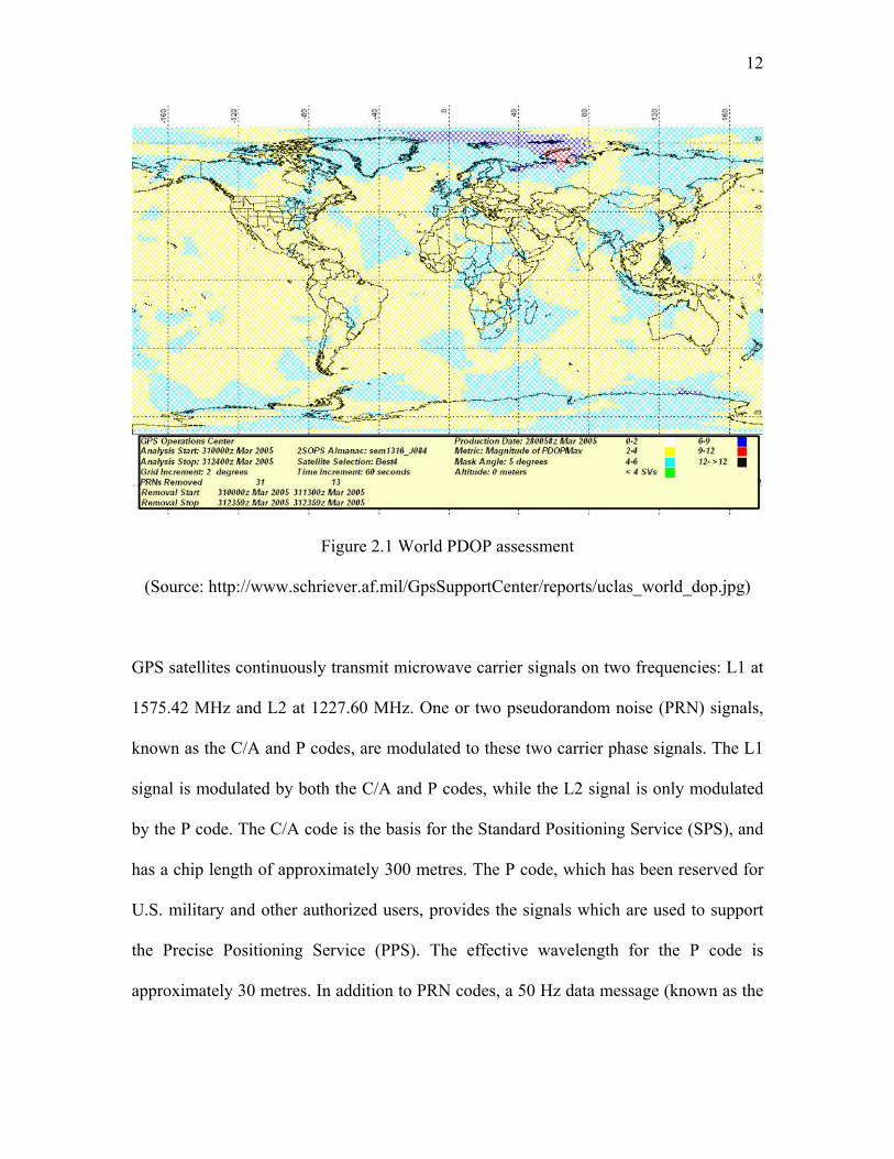
Full Operational Capability. Figure 2.1 shows the global coverage of the GPS

constellation. As can be seen from this figure, GPS constellation does not provide evenly

distributed position accuracy all around the world. Some parts of the world may even

experience significantly degraded position accuracy (red part).

12

Figure 2.1 World PDOP assessment

(Source: http://www.schriever.af.mil/GpsSupportCenter/reports/uclas_world_dop.jpg)

GPS satellites continuously transmit microwave carrier signals on two frequencies: L1 at

1575.42 MHz and L2 at 1227.60 MHz. One or two pseudorandom noise (PRN) signals,

known as the C/A and P codes, are modulated to these two carrier phase signals. The L1

signal is modulated by both the C/A and P codes, while the L2 signal is only modulated

by the P code. The C/A code is the basis for the Standard Positioning Service (SPS), and

has a chip length of approximately 300 metres. The P code, which has been reserved for

U.S. military and other authorized users, provides the signals which are used to support

the Precise Positioning Service (PPS). The effective wavelength for the P code is

approximately 30 metres. In addition to PRN codes, a 50 Hz data message (known as the

13

navigation message) is modulated onto the carriers and consists of status information,

satellite clock correction information, and satellite ephemerides.

The Operational Control System (OCS) consists of a master control station, monitor

stations, and ground control stations. The main tasks of the OCS are: tracking of the

satellites for orbit and clock determination and prediction, time synchronization of the

satellites, and uploading of the data message to the satellites (Hofmann-Wellenhof et al,

2001). There are five monitoring stations located at: Hawaii, Colorado Springs,

Ascension Island in the South Atlantic Ocean, Diego Garcia in the Indian Ocean, and

Kwajalein in the North Pacific Ocean. Each of these stations continuously measure

pseudoranges to all satellites in view and send these ranging measurements to the master

control station in Colorado Springs. The master control station processes the ranging

measurements in a Kalman filter every 15 minutes to determine satellite orbit and clock

corrections. These results form the content of the navigation messages to be uploaded to

the satellites (ibid).

2.2 GPS Time Frame

In this section, GPS pseudorange measurements were taken as an example to illustrate the

GPS time frame. By comparing the signal received from the satellite with an internally

generated signal, a receiver measures the time it takes for the signal to travel from the

satellite to the user. Pseudorange measurements are generated by multiplying this time-

delay measurement by the speed of light. The observation equation relating the

pseudorange measurements with the unknown parameters is given by Parkinson (1996):

14

( )srP c T T= − (2.1)

where P is the measured pseudorange measurements in metres, is the signal reception

time at the receiver,

rT

sT is the signal transmit time at the satellite and c is the speed of

light in a vacuum.

However, Eq. (2.1) only holds true in theory. The effects of the atmosphere on the signal

are neglected and it assumes that the transmit time and reception time refer to an absolute

time frame. In practice, the transmit time is implicitly embedded in the GPS signal and

refers to the satellite’s unique time frame. Similarly, the reception time is based on the

receiver’s time frame, i.e. the receiver’s local oscillator.

In the case of the satellite time frame, this time frame refers only to the satellite’s

onboard clock since it is the clock which drives the frequency synthesizer and code

generator required to generate the signal (ICD-GPS-200C, 2003). Since each satellite has

its own onboard clock and each one of these clocks slowly drifts over time, the signals

simultaneously received from several satellites belong to different time frames and the

differences between any two satellites’ individual time frame are not constant over time.

In the case of GPS, an “absolute” time frame is derived by averaging the master atomic

clocks at five ground monitoring stations (Francisco, 1996). The deviations of each

satellite’s onboard clock are continuously monitored by these stations, and a prediction

model for each satellite’s clock error is created based on these deviations (ICD-GPS-

200C, 2003):

15

(2.2) 20 1 2( ) (s

oc ocT a a t t a t t∆ = + − + − )

where sT∆ is the satellite clock offset, are the broadcast polynomial

coefficients, is the observation epoch and is the epoch to which the coefficients

refer.

0 1 2, ,a a and a

t oct

In addition, the relativistic effects due to the high altitude of the satellites and their high

velocity have to be corrected in the satellite transmit time. The corrected transmit time is

then given by (ICD-GPS-200C, 2003):

1/ 2

'2

2 sins s skT T T e a E

cµ

= −∆ + ⋅ ⋅1/ 2 (2.3)

where 'sT is the corrected transmit time, µ is the gravitational constant, is the speed of

light in vacuum, and are the semi-major axis, eccentricity and mean anomaly of

satellite orbit.

c

, , ka e E

Just as the transmit time refers to the satellite’s unique time frame, the measured

reception time refers to the receiver’s unique time frame. However, unlike the satellites

which use high quality atomic clocks, the receivers typically employ low cost quartz

oscillators. As a consequence, the clock offsets and drifts for the receivers can be larger

than those of the satellites.

Since the GPS receivers make observations to all visible satellites simultaneously, the

impacts of the receiver clock offset on all observations are identical. This allows the

solving of the receiver clock offset as an additional unknown parameter together with the

16

receiver coordinates in the least squares adjustment. Since the receiver clock offset drifts

over time, a new offset has to be estimated for each epoch.

In practice, since only reception time is explicitly known, one has to derive the

transmission time. If the reception time recorded by the receiver is , then the true time

of the measurement is with

rT

rT T− ∆ r rT∆ being the receiver clock offset. The transmit

time can be expressed as:

sr rT T T

cρ

= −∆ − (2.4)

where ρ is the true range between the satellite and receiver.

By replacing the true range ρ with the pseudorange measurement, one can derive:

( )ss sr

r r rp c T T pT T T T T

c c+ ∆ −∆

= −∆ − = − −∆ (2.5)

In Equation (2.5), the pseudorange observation noise is ignored, which is at the several

metre level (corresponding to a timing error of about 33 ns). The resulting error in the

transmit time calculation when using pseudorange observations contributes less than one

centimetre to the satellite position error (Radovanovic, 2002). Since the transmit time

usually ranges from approximately 67 ms to 90 ms (Remondi, 1984), a satellite position

error of up to 350 m could result if the correction for transmit time is not applied.

It should be emphasized that the transmitted navigation messages provide the user with

only a function from which the satellite position can be calculated in WGS84 as a

function of the transmission time. Usually, the satellite transmission times are unequal, so

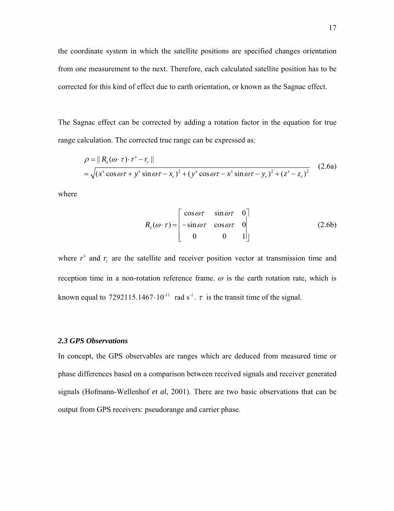
17

the coordinate system in which the satellite positions are specified changes orientation

from one measurement to the next. Therefore, each calculated satellite position has to be

corrected for this kind of effect due to earth orientation, or known as the Sagnac effect.

The Sagnac effect can be corrected by adding a rotation factor in the equation for true

range calculation. The corrected true range can be expressed as:

2 2

|| ( ) ||

( cos sin ) ( cos sin ) ( )

sz r

s s s s sr r

R r r2

rx y x y x y z

ρ ω τ

ωτ ωτ ωτ ωτ

= ⋅ ⋅ −

= + − + − − + z−

1

(2.6a)

where

cos sin 0

( ) sin cos 00 0

zRωτ ωτ

ω τ ωτ ωτ⎡ ⎤⎢ ⎥⋅ = −⎢ ⎥⎢ ⎥⎣ ⎦

(2.6b)

where sr and are the satellite and receiver position vector at transmission time and

reception time in a non-rotation reference frame.

rr

ω is the earth rotation rate, which is

known equal to . -11 -17292115.1467 10 rad s⋅ τ is the transit time of the signal.

2.3 GPS Observations

In concept, the GPS observables are ranges which are deduced from measured time or

phase differences based on a comparison between received signals and receiver generated

signals (Hofmann-Wellenhof et al, 2001). There are two basic observations that can be

output from GPS receivers: pseudorange and carrier phase.

18

The difference between these two types of observation is that the pseudorange is

generated by correlation between the satellite generated code and the identical copy of

the code generated inside the receiver, while the carrier phase is generated by comparing

the carrier frequency of the transmitted signal and the receiver generated replica. The

carrier phase is a more precise measurement mode. The principle advantage of carrier

phase measurement is that the phase of the carrier can be measured to better than 0.01

cycles which corresponds to millimetre precision (Hofmann-Wellenhof et al, 2001). On

the other hand, the pseudorange measurement noise is currently at the several decimetre

level (Langley, 1997).

However, Equation (2.1) only holds true in theory. The pseudorange and carrier phase

observations are both corrupted by many error sources such as receiver clock offsets,

satellite clock offsets, troposphere delay, ionospheric delay etc. Therefore, the complete

equations for pseudorange and carrier phase observations are given by:

( )( )sr orb trop ion multipath P PP c T T d d d dρ ε= + ∆ −∆ + + + + + (2.7)

( )( )sr orb trop ion multipathc T T d d d N d ϕ ϕϕ ρ λ= + ∆ −∆ + + − + ⋅ + +ε (2.8)

where,

P is the measured pseudorange in metres,

ϕ is the measured carrier phase in metres,

ρ is the true geometric range in metres,

c is the speed of light in vacuum in m/s,

sT∆ is the satellite clock error in seconds,

rT∆ is the receiver clock error in seconds,

19

orbd is the satellite orbit error in metres,

tropd is the tropospheric delay in metres,

iond is the ionospheric delay in metres,

λ is the signal wavelength in m/cycle,

N is the integer ambiguity in cycles,

( )multipath Pd is the multipath effect on pseudorange in metres,

( )multipathd ϕ is the multipath effect on carrier phase in metres,

Pε is the pseudorange measurement noise in metres, and

ϕε is the carrier phase measurement noise in metres.

In Equations (2.7) and (2.8), satellite orbit error, satellite clock error, receiver clock error,

and tropospheric error are frequency independent. The influence of these error sources on

pseudorange and carrier phase observations are the same from the same satellite on both

frequencies. On the other hand, the ionospheric error is frequency dependent, which is

proportional to the inverse of the squared frequency. Furthermore, the influence of

ionospheric error on pseudorange and carrier phase observations has the same magnitude

but with opposite sign, i.e. the pseudorange observations are delayed by the ionospheric

error while carrier phase observations are advanced by the ionospheric error.

In the context of this thesis, the double difference (DD) technique is used. The DD

observation equations are therefore discussed here. Figure (2.2) illustrates the typical

setup for double differencing.

20

Rover Station Base Station

Figure 2.2 Double difference concepts

By differencing between observations to the same satellite from the base and rover GPS

receivers, the satellite clock error is cancelled and the orbital, tropospheric, and

ionospheric errors are significantly reduced. The reduction of these errors depends on the

correlation of these errors in the observation between the base and rover stations. The

derived observation after differencing between receivers is known as the single difference

(SD). By further differencing the SD observations between different satellites, the double

difference observation is derived. After differencing between satellites, the receiver clock

error is completely eliminated.

The observation equations for double differenced pseudorange and carrier phase

observations are expressed as:

21

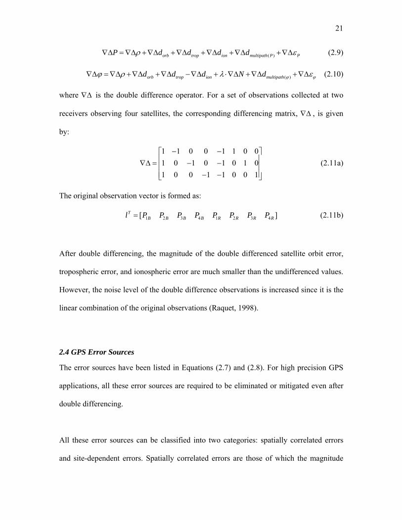
( )orb trop ion multipath P PP d d d dρ ε∇∆ = ∇∆ +∇∆ +∇∆ +∇∆ +∇∆ +∇∆ (2.9)

( )orb trop ion multipathd d d N d ϕ ϕϕ ρ λ∇∆ = ∇∆ +∇∆ +∇∆ −∇∆ + ⋅∇∆ +∇∆ +∇∆ε

⎥⎥

(2.10)

where ∇∆ is the double difference operator. For a set of observations collected at two

receivers observing four satellites, the corresponding differencing matrix, ∇∆ , is given

by:

(2.11a) 1 1 0 0 1 1 0 01 0 1 0 1 0 1 01 0 0 1 1 0 0 1

− −⎡ ⎤⎢∇∆ = − −⎢⎢ ⎥− −⎣ ⎦

The original observation vector is formed as:

(2.11b) 1 2 3 4 1 2 3 4[ ]TB B B B R R R Rl P P P P P P P P=

After double differencing, the magnitude of the double differenced satellite orbit error,

tropospheric error, and ionospheric error are much smaller than the undifferenced values.

However, the noise level of the double difference observations is increased since it is the

linear combination of the original observations (Raquet, 1998).

2.4 GPS Error Sources

The error sources have been listed in Equations (2.7) and (2.8). For high precision GPS

applications, all these error sources are required to be eliminated or mitigated even after

double differencing.

All these error sources can be classified into two categories: spatially correlated errors

and site-dependent errors. Spatially correlated errors are those of which the magnitude

22

increases with baseline length. These errors include satellite orbital error, tropospheric

error, and ionospheric error. Site-dependent errors are the errors which are unique to each

receiver or its environment. They are not correlated to baseline length and therefore can

not be cancelled through DD. These errors include multipath and receiver noise.

As has been discussed previously in this chapter, satellite clock error and receiver clock

error will not be repeated here. All the above mentioned error sources will be discussed in

the following paragraph.

2.4.1 Satellite Orbit Error

As previously mentioned, to position with GPS, the coordinates of the GPS satellites are

generally assumed to be known. These coordinates are normally expressed in terms of an

ephemeris, which gives a mathematical description of where a satellite is at a given time

(Roulston et al, 2000). The satellite orbital error is a result of the discrepancy between the

computed coordinate from the ephemeris and its true value.

The effect of satellite orbital error on differential positioning can be given using the

following rule of thumb (Beutler, 1992):

orbddbb ρ= (2.12)

where is the baseline error. b is the baseline length. is the satellite orbit error

and

db orbd

ρ is the distance from satellite to the receiver. The computed satellite coordinates

from broadcast ephemeris have a standard deviation of approximately 3 m (Roulston et al,

23

2000). Assuming an average satellite-receiver distance of 20200 km, the effect of satellite

orbital error on differential positioning is approximately 0.099 parts per million (ppm). It

can be concluded that the effect of satellite orbit error on differential positioning for a

baseline up to 50 km is approximately 5 mm and thus can be neglected in most cases.

Moreover, the configuration of the satellite orbit has the following effects on GPS

positioning (Rizos, 1999):

Height is a relatively weakly determined component, mainly because there are no

satellites below the horizon.

The East-West (longitude) component is slightly weaker than the North-South

(latitude) component because of the motion of satellites (particularly in equatorial

regions.

There are two basic types of satellite orbit information: broadcast and post-processed

ephemerides. The broadcast ephemerides, which are available in the GPS Navigation

Message, are predicted from past tracking information. Therefore, they can be used for

real time applications. Post-processed ephemerides are orbit representations valid only

for the time interval covered by the tracking data. Obviously this information is not

available in real time as there is a delay between the collection of the data, transmission

of the data to the computing centre, the orbit determination process and the subsequent

distribution to GPS users (Rizos, 1999). Post-processed ephemerides, which come in

several forms, are more accurate than broadcast ephemerides. The IGS post-processed

ephemerides products demonstrated accuracies well below the metre level to several

24

centimetres (Roulston et al, 2000). Because of the high precision of the post-processed

ephemerides, they are widely used in various high precision GPS applications. In the

context of this thesis, IGS final orbit product is used for all GPS data processing.

2.4.2 Tropospheric Error

The troposphere is the portion of the atmosphere extending up to 60 km above the Earth’s

surface. When the GPS signal travels through the troposphere, its path will bend slightly

due to the refractivity of the troposphere. The change of the refractivity from free space

to the troposphere causes the speed of the GPS signal to slow down, which causes a delay

in the GPS signal. This tropospheric delay is a function of temperature, pressure, and

relative humidity. Measurement of these quantities at widely spaced (greater than 10 km)

monitoring stations would be ineffective owing to their short spatial correlations (Kaplan,

1996).

There are two components in the tropospheric delay: dry and wet component. The effect

of these two components on the propagation delay of the GPS signals has quite different

characteristics. The dry component causes a delay of around 2.3 m in the zenith direction

depending on local temperature, pressure, and humidity. The dry component induced

delay is quite stable over time (varies only 1% in a few hours) and thus can be very well

predicted using existing models. The wet component of the zenith delay is generally

much smaller (between 1 and 80 cm at zenith direction), and is very unpredictable. It may

change by as much as 10% to 20% in a few hours (Spilker, 1994).

25

Generally, tropospheric delay can be modelled very well. It was found that the

contribution of the troposphere to the differential positioning error budget varies typically

from 0.2 to 0.4 ppm after applying a model (Lachapelle and Cannon, 2004). For baselines

up to 25 km, the residual tropospheric delay is approximately 1 cm.

However, to achieve centimetre or even millimetre accuracy, either a tropospheric model

must be applied or the residual tropospheric delay must be estimated as an additional

parameter. There are quite a number of tropospheric delay models available, e.g.

Hopfield (1970, 1972), Saastamoinen (1972), and Lanyi (1984). The Hopfield

tropospheric delay model and Saastamoinen tropospheric model are the most frequently

used and they give comparable results in most situations. For low elevation satellites, the

Saastamoinen model produces slightly better results than the Hopfield model (Spilker,

1994).

2.4.3 Ionospheric Error

The ionosphere is the layer of the atmosphere that extends from 60 to over 1000 km of

height above the Earth’s surface. At times, the range errors of the troposphere and the

ionosphere are comparable, but the variability of the Earth’s ionosphere is much larger

than that of the troposphere, and it is more difficult to model (Klobuchar, 1996). The

first-order carrier phase error I (in metres) caused by the ionosphere is given as (Seeber,

1993; Hofmann-Wellenhof et al, 2001):

2

40.3I TECf

= − (2.13)

where 40.3 is an empirically derived constant with units of m3/s2/electrons, TEC

26

represents the Total Electron Content along the signal path in units of electrons/m2, and f

is the L1 or L2 carrier frequency.

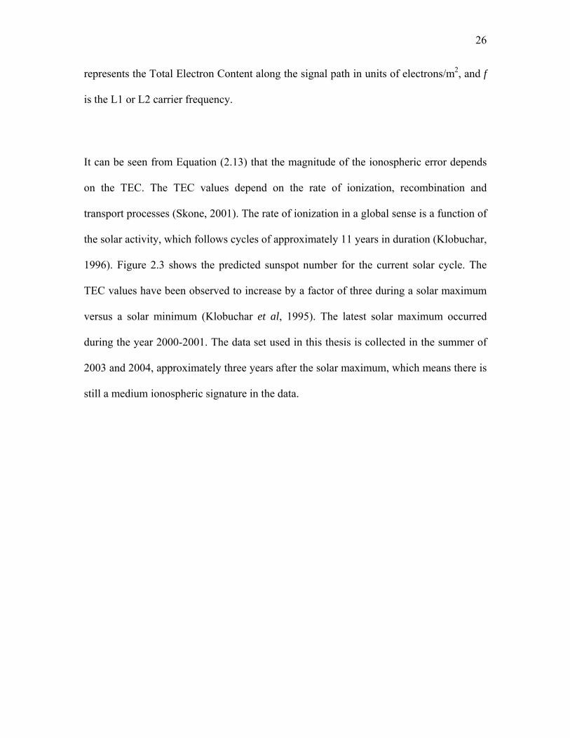
It can be seen from Equation (2.13) that the magnitude of the ionospheric error depends

on the TEC. The TEC values depend on the rate of ionization, recombination and

transport processes (Skone, 2001). The rate of ionization in a global sense is a function of

the solar activity, which follows cycles of approximately 11 years in duration (Klobuchar,

1996). Figure 2.3 shows the predicted sunspot number for the current solar cycle. The

TEC values have been observed to increase by a factor of three during a solar maximum

versus a solar minimum (Klobuchar et al, 1995). The latest solar maximum occurred

during the year 2000-2001. The data set used in this thesis is collected in the summer of

2003 and 2004, approximately three years after the solar maximum, which means there is

still a medium ionospheric signature in the data.

27

Figure 2.3 Predicted sunspot number for the current solar cycle

(Source: http://science.nasa.gov/ssl/pad/solar/images/ssn_predict_l.gif)

In addition to the large scale variation with solar cycle, the TEC presents the following

variation characteristics (Skone, 2003):

Maximum TEC occurs at 14:00 local time and TEC can be asymmetric with a

secondary maximum at 22:00 local time and a minimum before sunrise.

The lowest TEC values are in the summer (for the Northern Hemisphere) and

maximum near the equinoxes (March and October). This is opposite for the Southern

Hemisphere, i.e. lowest in the winter and maximum in the summer. The TEC values

are 2-3 times higher in winter than in summer.

28

The two maxima are at ±10° from the magnetic equator, in the region under the so-

called equatorial anomaly.

There are some models available to compensate the ionospheric delay. Klobuchar (1986)

introduced a model that is being used by the GPS Control Center as part of the navigation

message broadcast by the GPS satellites. This model utilizes a cosine function to

represent the diurnal ionospheric error. It has been shown to be effective in removing

around 50% (RMS) of the total error. This model is helpful for improving SPS

performance. However, to achieve centimetre accuracy, it is not sensitive enough and it is

not therefore used in carrier phase applications.

Although the ionospheric error is hard to compensate for by applying models, it can be

eliminated by making use of its dispersive property. From Equation (2.13), it can be seen

that the ionospheric error on L1 and L2 is different and is proportional to the inverse of

the square of frequency. This dispersive property allows the formation of a very

important carrier phase combination, the ionosphere-free (IF) combination, in which the

ionospheric error is removed.

The contribution of residual ionospheric error to differential positioning has been

reported by Alves et al (2002) to be approximately 2 ppm on geometry-free combination

observations on baselines up to 50 km under ionospheric quiet conditions. During the

time of solar maximum, the contribution of residual ionospheric error to differential

positioning error budget can increase by a factor of three (Lachapelle and Cannon, 2004).

29

2.4.4 Multipath

Multipath is the interference of a reflected GPS signal with the line-of-sight GPS signal.

It distorts the signal modulation and thus degrades the measurement accuracy (Braasch,

1996).

The theoretical maximum multipath bias that can occur in the pseudorange data is

approximately half the code chip length or 150 m for C/A code ranges and 15 m for P

code. The carrier phase multipath is much smaller than that of the pseudorange, with a

maximum magnitude of one quarter of a carrier wavelength, i.e. 5 cm for L1 and 6 cm for

L2 (Cannon and Lachapelle, 2003). However, in practical applications, the reflected

signal is attenuated to some extent and the typical phase multipath values are more on the

order of 1 cm or less (Lachapelle and Cannon, 2004).

Multipath effects have to be carefully treated in GPS data processing to achieve very high

position accuracies. Several methods for effectively reducing multipath effect have been

developed. Examples include the mitigation of GPS code and carrier phase multipath

effects using a multi-antenna system (Ray, 2000), multipath mitigation via day-to-day

correlation analysis (Radovanovic, 2000), and multipath mitigation by making use of

signal-to-noise ratio information (Brunner et al, 1999). Moreover, by using a chokering

antenna in the field data collection, multipath effects can be greatly reduced (Lachapelle

and Cannon, 2004).

The multipath mitigation via day-to-day correlation was considered to be the most

effective method for mitigation multipath for static GPS data. This method will be

30

implemented and used for the data processing in this thesis to improve station positioning

accuracy (See chapter 5).

2.5 Precise Levelling and its Error Sources

Early levelling was done with crude instruments that had a provision for sighting along a

water surface or by some mechanical application of a plumb line (Berry, 1976). Today,

more sophisticated equipment enables levelling to achieve very high accuracies. This new

equipment depended on the invention of three important items: (1) the telescope invented

by a Dutch optician by the name of Lippershey in 1608; (2) the reticle with cross wires

and the ocular invented by Johann Kepler in 1611 and (3) the level vial invented by

Melchisedech Thevenot in 1666 (Gareau, 1986). Moreover, by applying laser technology

in the instrument and the improvement in manufacturing techniques of the invar rod in

recent days, the performance of the levelling is significantly improved.

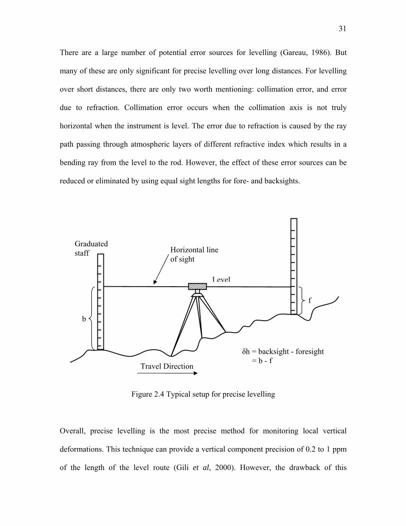
Levelling provides a means of accurately measuring of the height difference between two

points that are some tens of metres apart. A level is setup on a tripod and levelled so that

the line of sight is horizontal. A precise graduated rod is held vertically over the first

point and a reading is made from the level, which is called a backsight. Another rod is

then held vertically over the second point and a further reading is made, which is called a

foresight. The difference between the two readings is the difference in height between the

two points. Figure (2.4) illustrates the typical setup for precise levelling.

31

There are a large number of potential error sources for levelling (Gareau, 1986). But

many of these are only significant for precise levelling over long distances. For levelling

over short distances, there are only two worth mentioning: collimation error, and error

due to refraction. Collimation error occurs when the collimation axis is not truly

horizontal when the instrument is level. The error due to refraction is caused by the ray

path passing through atmospheric layers of different refractive index which results in a

bending ray from the level to the rod. However, the effect of these error sources can be

reduced or eliminated by using equal sight lengths for fore- and backsights.

Graduated staff

Figure 2.4 Typical setup for precise levelling

Overall, precise levelling is the most precise method for monitoring local vertical

deformations. This technique can provide a vertical component precision of 0.2 to 1 ppm

of the length of the level route (Gili et al, 2000). However, the drawback of this

Travel Direction

f

b

Horizontal line of sight

Level

δh = backsight - foresight = b - f

32

technique is obvious at the same time. First, precise levelling can only provide

information in one dimension. Second, levelling must be initiated from a stable

monument located outside the deformation area in most cases. The result may be that the

level route goes up to several kilometres, which makes the levelling work laborious, often

slow, and subject to the propagation of levelling errors. These reduce the overall

effectiveness of this technique. However, for some potential relative networks, trend

signal analysis (Kenselaar and Quadvlieg, 2001) allows a network that is constrained

using one of the unstable benchmarks in the test area.

It is important to note that the heights obtained from levelling are orthometric heights

while the heights obtained from GPS are ellipsoidal heights. The relationship between

these two height types is given by (Heiskanen and Moritz, 1967):

0h H N− − = (2.14)

where h is the ellipsoidal height, H is the orthometric height and N is the geoidal

undulation obtained from a regional gravimetric geoid model or a global geopotential

model. The relationship of the two height types are also illustrated in figure (2.5):

33

Figure 2.5 Relationship between ellipsoidal, geiod and orthometric heights

(Fotopoulos, 2003)

When comparing heights obtained from GPS and heights obtained from precise levelling,

one has to note that they belong to different height systems. However, for a very small

area (a circle with a diameter of 70 metres), the magnitude of change of N is quite small

and thus can be neglected. Consider the variation in gravitational acceleration that would

be observed over a simple model. For this model, let’s assume that the only variation in

density in the subsurface is due to the presence of a small ore body. Let the ore body have

a spherical shape with a radius of 10 meters, buried at a depth of 25 meters below the

surface, and with a density contrast to the surrounding rocks of 0.5 grams per centimetre

cubed (see Figure 2.6). The maximum value of the gravity anomaly is quite small, 0.025

mGals (1 Gal = 1 cm/sec2, 1 Gal = 1,000 milligals) for this example. This maximum

34

variation of gravity anomaly transferred into the variation of geoid undulation is only 2-3

mm. Therefore, the variation of geoid undulation within a small area (a circle with a

diameter of 70 metres) can be neglected. Because of the high accuracy of precise

levelling in height component, levelling results can be used as ground truth to examine

the performance of GPS levelling in a small area (a circle with a diameter of 70 metres).

Figure 2.6 A simple model illustrating the variation of gravity anomaly

(Source: http://gretchen.geo.rpi.edu/roecker/AppGeo96/lectures/gravity/simpmod.html)

35

2.6 Deformation Monitoring Overview

Deformation monitoring is used for many applications, including monitoring of large

structures such as dams and bridges, steep slopes and embankments, and measuring

terrain subsidence due to sub-surface mineral extraction (Caspary, 1987). A deformation

survey measures the change of the target object or area with respect to time using a

network of points. It is assumed that the measurements are made faster than the

deformation process itself and repeated measurements are often done to determine

temporal trends. This is done using different geodetic methods for a one-, two- or three-

dimensional monitoring.

There are two types of monitoring networks depending on the distribution of points. If

the stations around and close to the object, called reference points, can be located on

points that will remain stable throughout the period of deformation monitoring, these can

be used for network datum definition (Tait, 2004). This is known as an absolute (or

reference) monitoring network (Tait, 2004). In this case, movements of the target object

or area are determined with respect to the reference points.

A second type of network is called a relative network (Biacs, 1989). In this case, there is

no assumption regarding the stability of any survey stations whereby all the points in the

network may move. It means none of the points can be used for datum definition. The

obvious choice for the datum in a relative network is inner constraints (Tait, 2004).

Therefore, the derived point coordinates are solely based on observations. All the points

are treated as object points and only relative movements with respect to the centroid of

network can be estimated.

36

For a relative network, it is not possible to model absolute rigid body movements, which

is required for most deformation monitoring applications (Caspary, 1987). In this case, it

is necessary to turn the relative network into an absolute monitoring network. The most

important task in this case is to define points which are stable over time that can be used

as reference points. Test statistics can be introduced to test the stability of network points,

which are known as congruency tests (Tait, 2004). There are three stages: Global

congruency test, congruency testing of partial networks, and the detection of movement

of points (Tait, 2004). These tests are based on the information from individual epoch

coordinate estimates and, critically, on the variance-covariance of the estimates. Thus the

sensitivity of the test relies upon the quality of the observations, the shape of the network

and the network datum (Tait, 2004).

GPS deformation monitoring applications have shown that it is capable of monitoring

sub-centimetre deformations when using carrier phase measurements (e.g. Hartinger and

Brunner, 1998). There exist many applications to apply GPS for high accuracy

positioning and deformation monitoring. In most cases, such applications are of small

spatial extent (<10 km) (Radovanovic, 2000). These applications include bridge

monitoring (Wieser and Brunner, 2002), dam deformation monitoring (Hudnut, 1996),

structure deformation monitoring under wind load (Guo and Ge, 1997), and landslide

monitoring (Hartinger and Brunner, 2000).

37

The attainable accuracy for a GPS-based deformation monitoring system is limited by

many location dependent errors. Recent work on the effects of location dependent

variables such as satellite geometry (Meng et al, 2004), tropospheric effects (Roberts and

Rizos, 2004), and ionospheric effects (Janssen et al, 2001) have mitigated these errors by

employing an optimised strategy for data capture and processing.

Furthermore, Continuous GPS monitoring techniques have shown great success in many

long-term deformation monitoring applications, for instance the Continuous GPS

monitoring of structural deformation at Pacoima Dam (Hudnut et al, 2001). In addition,

there are those that have been established in sub-arctic areas, for instance the SWEPOS

system (Hedling et al, 2001). The advantage of the Continuous GPS monitoring

technique is that it allows continuous study of all the site-dependent errors and offers

real-time positioning information. In addition, no human interference is needed in this

case.

Overall, GPS has shown very good performance in many deformation monitoring

applications. Examples include the Pacoima Dam deformation monitoring system which

has shown that GPS can provide real-time positioning accuracies of 1 cm in horizontal, 2

cm in vertical and post-processed positioning accuracies of 2-4 mm in horizontal and 6-8

mm in vertical (Hudnut and Behr, 1998). Also, a bridge deformation monitoring system

developed by the Graz University of Technology has shown that the precision of the GPS

results is about 2 mm for the horizontal coordinates and 4 mm for the height (Wieser and

Brunner, 2002).

38

CHAPTER 3

PROJECT BACKGROUND

This chapter gives an overview of the target area, where the research described in this

thesis is related to, and its subsidence issue. Previous feasibility studies of the most

appropriate method for subsidence monitoring in the target area are summarized as part

of the project background. The problems to be investigated are reiterated as project

objectives at the end of this chapter.

3.1 Subsidence Issue in the Target Area

Oil and gas extraction in permafrost (continuously frozen soil) areas causes vertical

surface displacements that have in the past caused serious environmental issues, such as

massive subsidence and land slides (Rempel, 1970). To avoid potential environmental

disasters during oil and gas extraction, such vertical subsidence has to be accurately

monitored.

The target area, Niglintgak Island, lies approximately 150 kilometres north of Inuvik at a

latitude of 69° 20’ North and a longitude of 135° 20’ West. Figure 3.1 shows a map of

Canada highlighting both the area of interest, and the distribution of permafrost. Much of

the subsidence is expected to form beneath the Kumak Channel to the south of the island

(Figure 3.2).

39

The target area is characterized by continuous permafrost to depths of up to 600 m (Smith

et al, 2001). The annual freeze/thaw of the active layer above the permafrost in this area

has been observed at the 20 cm level (Mackay et al, 1979), with a wide variation in

timescale dependant on such factors as annual snow cover, atmospheric conditions, and

vegetation growth.

Figure 3.1 The distribution of permafrost in Canada and areas of the Niglintgak and

Taglu gas reservoirs (Tait et al, 2004)

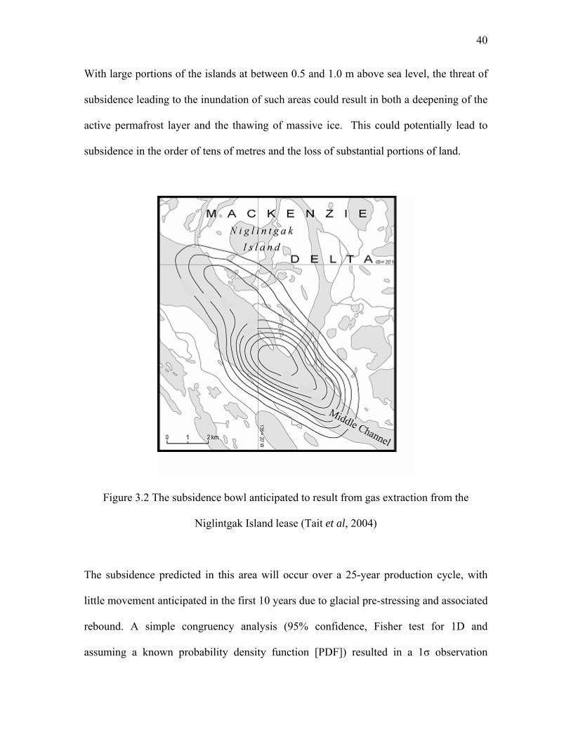
40

With large portions of the islands at between 0.5 and 1.0 m above sea level, the threat of

subsidence leading to the inundation of such areas could result in both a deepening of the

active permafrost layer and the thawing of massive ice. This could potentially lead to

subsidence in the order of tens of metres and the loss of substantial portions of land.

Figure 3.2 The subsidence bowl anticipated to result from gas extraction from the

Niglintgak Island lease (Tait et al, 2004)

The subsidence predicted in this area will occur over a 25-year production cycle, with

little movement anticipated in the first 10 years due to glacial pre-stressing and associated

rebound. A simple congruency analysis (95% confidence, Fisher test for 1D and

assuming a known probability density function [PDF]) resulted in a 1σ observation

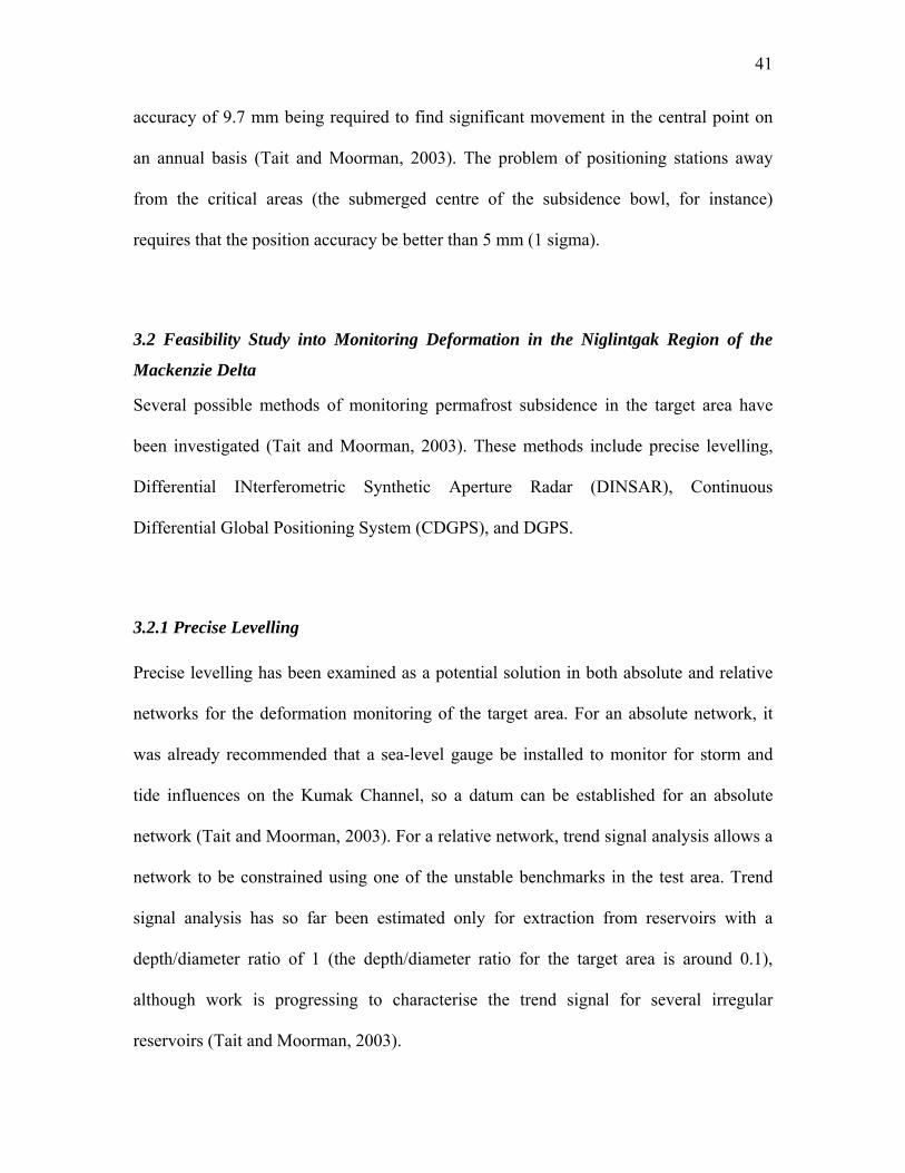
41

accuracy of 9.7 mm being required to find significant movement in the central point on

an annual basis (Tait and Moorman, 2003). The problem of positioning stations away

from the critical areas (the submerged centre of the subsidence bowl, for instance)

requires that the position accuracy be better than 5 mm (1 sigma).

3.2 Feasibility Study into Monitoring Deformation in the Niglintgak Region of the

Mackenzie Delta

Several possible methods of monitoring permafrost subsidence in the target area have

been investigated (Tait and Moorman, 2003). These methods include precise levelling,

Differential INterferometric Synthetic Aperture Radar (DINSAR), Continuous

Differential Global Positioning System (CDGPS), and DGPS.

3.2.1 Precise Levelling

Precise levelling has been examined as a potential solution in both absolute and relative

networks for the deformation monitoring of the target area. For an absolute network, it

was already recommended that a sea-level gauge be installed to monitor for storm and

tide influences on the Kumak Channel, so a datum can be established for an absolute

network (Tait and Moorman, 2003). For a relative network, trend signal analysis allows a

network to be constrained using one of the unstable benchmarks in the test area. Trend

signal analysis has so far been estimated only for extraction from reservoirs with a

depth/diameter ratio of 1 (the depth/diameter ratio for the target area is around 0.1),

although work is progressing to characterise the trend signal for several irregular

reservoirs (Tait and Moorman, 2003).

42

Despite the high accuracy of precise levelling for height measurement, there are several

drawbacks of applying precise levelling for the target area. Since a great deal of the area

has large water bodies (>2 km), over which to make precise levelling measurement is

very difficult. In addition, it does not provide planimetric measurements at all, which is

insufficient for monitoring horizontal movements. For the above reasons, precise

levelling is not recommended in this case.

3.2.2 DINSAR

DINSAR has the potential to detect sub-centimetre vertical movements (Wang and Li,

1999). However, the feasibility study noted two problems with DINSAR for monitoring

in the Mackenzie Delta (Tait et al, 2004):

1. DINSAR relies on the reflection of microwave radiation remaining constant for

the area of study. If the scattering properties of the area change between satellite

acquisitions due to changes in surface wetness or vegetation growth, this alters the

phase of the returned radiation. Such phase alteration with time, known as

temporal decorrelation, makes deformation analysis difficult or impossible. Even

in regions with less vegetation than the Mackenzie Delta, it was found that

between RADARSAT-1 images with a 24 day separation there was too little

coherence to generate measurements of vertical displacement (Moorman and

Vachon, 1998; Moorman et al, 2003).

43

2. If a deformation map of the area can be generated using DINSAR, this map is of

the surface of the permafrost. In the Mackenzie Delta the active layer of the

permafrost has been observed to cause heave and settlement of up to 20 cm on an

annual basis (Mackay et al, 1979). This is influenced by climatic conditions,

vegetation cover, and soil type. This makes estimating true subsidence from

measurement of the elevation of the surface itself impossible without an adequate

model of the active layer heave. Permafrost models are anticipated to be accurate

to 1-2 cm (Tait and Moorman, 2003).

Since the planimetric deformation may impose shear on production platforms, both

vertical and planimetric measurements of deformation are desired in this case. In the case

of DINSAR, the planimetric accuracy is much lower than vertical measurement accuracy.

It can not provide the desired full 3 dimensional monitoring, which makes it less

attractive in this case.

3.2.3 CDGPS

Recognizing the success of Continuous GPS monitoring technique (see Section 2.6), it

was also assessed for application in the target area. For continuous monitoring, several

factors have to be taken into consideration: power supply for GPS receivers, internet

availability to upload data to the server, infrastructure for maintenance, and animal

activity. In addition, because the target area is in the far north of Canada, weather is a big

issue, including high winds and extreme cold. Additional devices are generally needed to

prevent GPS antennas from icing. The requirements for continuous GPS monitoring are

44

hard to meet in the target area. This approach was considered unfeasible since

implementing a relatively large number of such stations, together with the problem of

lack of communications in the target area, presented serious logistical and cost issues

(Tait and Moorman, 2003).

3.2.4 DGPS

DGPS is a well established fully 3-dimensional measurement method which allows the

estimation of deformation parameters at the centimetre level and at the millimetre-level in

special cases (Hartinger and Brunner, 1998; Beutler et al, 2001). Phase-Centre-Variation

of the receiving antenna and multipath effects have been identified in the past as the

major station-dependent causes of errors in precise engineering measurement using

DGPS (Wübbena et al, 2000). However, DGPS also has challenges specific to the target

area. In particular, the effects of ionospheric activity and relatively poor satellite

geometry in the Arctic region might also contribute to the error budget over longer

baselines, even when using an ionosphere-free combination during processing.

In order to illustrate the satellite geometry in the target area, the number of available

satellites, dilution of precision (DOP) values (PDOP, HDOP, and VDOP), and the

skyplot over 24 hours at the INVK station generated from a GPS planning tool as well as

from original data processing for the date of Jul 8th, 2004 are plotted and shown in Figure

3.3. The elevation cut-off angle was set to 10 degrees.

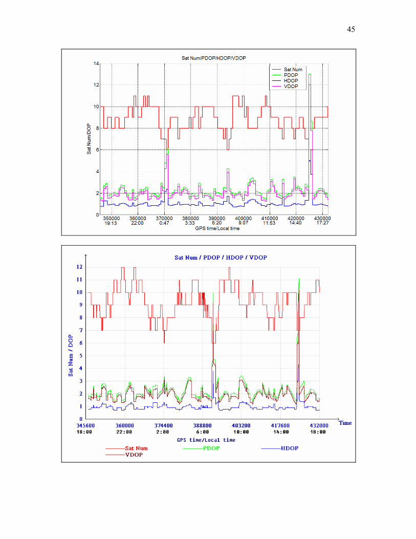
45

46

10

20

40

60

80

Figure 3.3 DOP values and number of available satellites generated from GPS planning

tool (top) and GPS data processing (middle) and skyplot (bottom) over 24 hours at INVK

station

For comparison purposes, the number of available satellites, DOP (PDOP, HDOP, and

VDOP) values generated from GPS planning tool as well as original data processing and

the skyplot over 24 hours at another, mid-latitude, IGS station near Calgary, PRDS, were

plotted and shown in Figure 3.4. Elevation cut-off angle was again set to as 10 degrees.

47

48

10

20

40

60

80

Figure 3.4 DOP values and number of available satellites generated from GPS planning

tool (top) and GPS data processing (middle) and skyplot (bottom) over 24 hours at PRDS

station

By looking at the skyplot and DOP values over these two stations, two observations were

made:

1. There are no satellite passes overhead the INVK station and the elevation angle of

the highest available satellite is approximately 75 degrees. This is not the case for

the PRDS station. According to Meng et al (2004), an optimal constellation to

minimize the DOP values is given by a GPS satellite passing directly overhead of

the observation station, with other satellites scattered around the horizon with

associated low elevation angles. With the current GPS constellation, the target

area will experience degraded satellite geometry than that of a mid-latitude area.

49

2. The horizontal DOP (HDOP) values for these two stations are at the same level,

around 1, except for several spikes at INVK station. The vertical DOP (VDOP)

values for PRDS station are slightly better than INVK station. Most of the VDOP

values at INVK station are between 2 and 3, while most of the VDOP values at

PRDS station are below 2. The VDOP value at INVK station may even go up to

10 sometimes. Besides, the VDOP values at the PRDS station have much less

variations than that of the INVK station.

The level of global ionospheric activity can be quantified using the conventional space

weather index Kp. This index is based on measurements of magnetic field variations at

13 approximately equally longitude-spaced sub-auroral stations to produce the planetary

Kp index at three-hour intervals, with values ranging from 0 (quiet) to 9 (extreme)

(Skone, 2003). Such indices provide an approximate measure of global ionospheric

activity at higher latitudes. Figure 3.5 shows the Kp index for a quiet day (14 July, 2004)

and Figure 3.6 shows a day of significant ionospheric disturbance (25 July, 2004).

50

Figure 3.5 Kp index for a quiet day, 14 July, 2004

(Source: http://www.sec.noaa.gov/ftpmenu/plots/2004_plots/kp.html)

Figure 3.6 Kp index for a day of significant ionospheric disturbance, 25 July, 2004

(Source: http://www.sec.noaa.gov/ftpmenu/plots/2004_plots/kp.html)

51

3.3 Project Objectives

The overall goal of this project was to analyse and reduce the location dependent errors in

the use of DGPS levelling in the north of Canada, as other researchers have done

in different environments (Section 2.6). In addition, for any derived monument-based

deformation monitoring method, the stability of the monument is a fundamental

requirement, which must be quantified and taken into account in the total error budget

(Kenselaar and Quadvlieg, 2001). For the target area, an area of relatively high

heave/settlement, a relatively large signal is expected. To establish a complete error

budget for the deformation monitoring in the target area, the long-term stability of

different survey monument in permafrost has to be characterized and quantified.

The challenges for GPS in the target area mainly lie on two aspects. First, in the far north,

no GPS satellites pass overhead of the observation stations and all the satellites scatter

around the horizon, in which case the satellite geometry is degraded compared to the

mid-latitude case. Another site-specific problem occurs due to the increased ionospheric

activity in the north compared to mid-latitudes, and this is particularly exacerbated by he

low angle of the satellites and subsequent increased path-length of the GPS signals. This

leads to increased loss of signal (cycle slips) as well as path delays due to ionospheric

activity (Skone et al, 2001).

In order to assess the ability of GPS for deformation monitoring in the target area, the

attainable accuracy of GPS, especially height component, in the target area has to be

examined. The impact of different error sources influencing GPS positioning accuracy

has to be examined. These error sources include: tropospheric delay, antenna phase centre

52

variation, ionospheric delay and multipath. In addition, the impact of satellite geometry

on GPS positioning accuracy is to be examined.

53

CHAPTER 4

PRE-RESEARCH FOR THE TARGET AREA

Prior to carrying out the field campaign in the target area, some initial research was

carried out in order to characterize two types of error sources: antenna phase centre

variation and multipath. In this chapter, an overview of these error sources is given, and

experiments undertaken to characterize and/or mitigate these two types of error sources

are described.

4.1 Antenna Phase Centre Variation

4.1.1 Introduction

Differential GPS solutions are obtained from a baseline vector which extends from a

station with known coordinates and constrained to a station whose position is to be

determined. Once a baseline vector is determined, it is assumed to be a vector between

the antenna phase centres of the base and rover stations. However, the phase centre of a

GPS antenna is neither a physical point nor a stable point (Mader, 1999). For any given

GPS antenna, the phase center will change with the changing direction of the signal from

a satellite. Ideally, most of this PCV depends on satellite elevation. Azimuthal effects are

only introduced by the local environment around each individual antenna site (Mader,

1999).

These phase centre variations affect the antenna offsets that are needed to connect GPS

measurements to physical monuments. If this variation is ignored, the measured baseline

54

will be between the average phase centres of the two antennas. These average phase

centre locations are a weighted average of all the individual phase centers for each of the

measurements included in the solution through least squares estimation. Antenna phase

centre variation has become, besides tropospheric and multipath errors, the most limiting

factor to achieve a breakthrough to the next accuracy level for precise GPS measurements

(Wübbena et al, 2000). Ignoring these phase centre variations can lead to up to 10 cm

vertical errors (Mader, 1999).

A full description of GPS antenna phase centre behaviour contains information on

(Wübbena et al, 2000):

• Antenna Reference Point (ARP)

• 3D mean phase center offset referring to the ARP

• PCV for L1 and L2 with respect to the given offsets

Figure 4.1 illustrates the relationship between the ARP, mean offset and phase centre

variation. The dimension arrows in this figure illustrate how the antenna PCV was related

to the ARP.

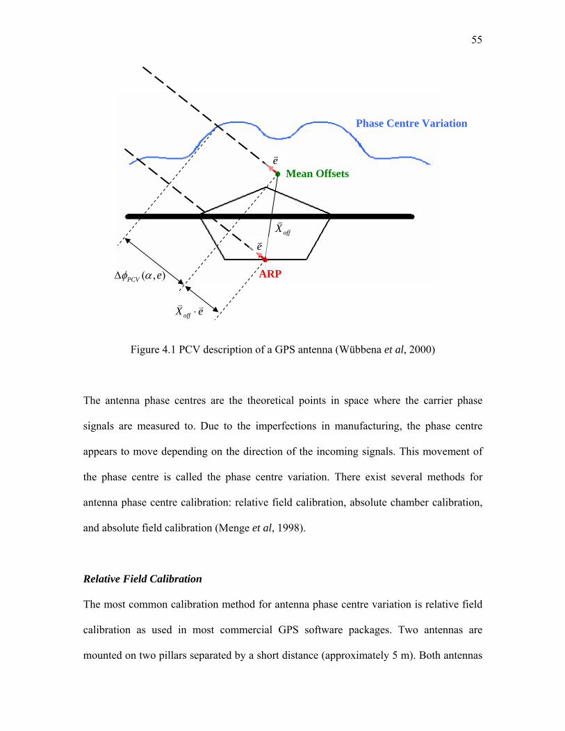
55

SV

Figure 4.1 PCV description of a GPS antenna (Wübbena et al, 2000)

The antenna phase centres are the theoretical points in space where the carrier phase

signals are measured to. Due to the imperfections in manufacturing, the phase centre

appears to move depending on the direction of the incoming signals. This movement of

the phase centre is called the phase centre variation. There exist several methods for

antenna phase centre calibration: relative field calibration, absolute chamber calibration,

and absolute field calibration (Menge et al, 1998).

Relative Field Calibration

The most common calibration method for antenna phase centre variation is relative field

calibration as used in most commercial GPS software packages. Two antennas are

mounted on two pillars separated by a short distance (approximately 5 m). Both antennas

Mean Offsets

Phase Centre Variation

ARP

e

offXe

( , )PCV eφ α∆

offX e⋅

56

are connected to GPS receivers which use a Rubidium oscillator as an external frequency

standard. Because the PCV is determined using L1 or L2 single differences rather than

double differences, the receiver clock error can not be cancelled out. The Rubidium

oscillator is used to mitigate the receiver clock error variation. Using single differences

will determine the PCV directly rather than from different satellites at different elevations.

A 10 degree cutoff angle was used for tracking GPS signals by most agencies that carried

out this type of calibrations (Mader, 1999).

The antenna PCV is determined separately for L1 and L2. To calibrate the antenna PCV,

a reference antenna is selected, typically the JPL D/M+crT antenna, for which the PCV of

this reference antenna are set to zero and the offsets are also fixed. The calibration is then

referenced to this antenna. In the first stage of the calibration, a second JPL D/M+crT is

mounted on the test pillar, so the L1 and L2 phase centre of this antenna on the test pillar

can be determined. These positions are then used as a priori information for the L1 and

L2 antenna phase centres of the remaining test antennas. From the solution of the test

antennas, the difference from the a priori position can be calculated which can then be

used to calculate the location of the test antenna phase center relative to the reference

antenna.

The drawback of this type of calibration is as follows: Firstly, the antenna PCV for the

reference antenna is set to zero, which is not true in reality. Secondly, the calibration is

with respect to a particular circumstance (i.e. the product is dependent on the satellite

constellation, the location of the test site and the multipath effects of the test site). Lastly,

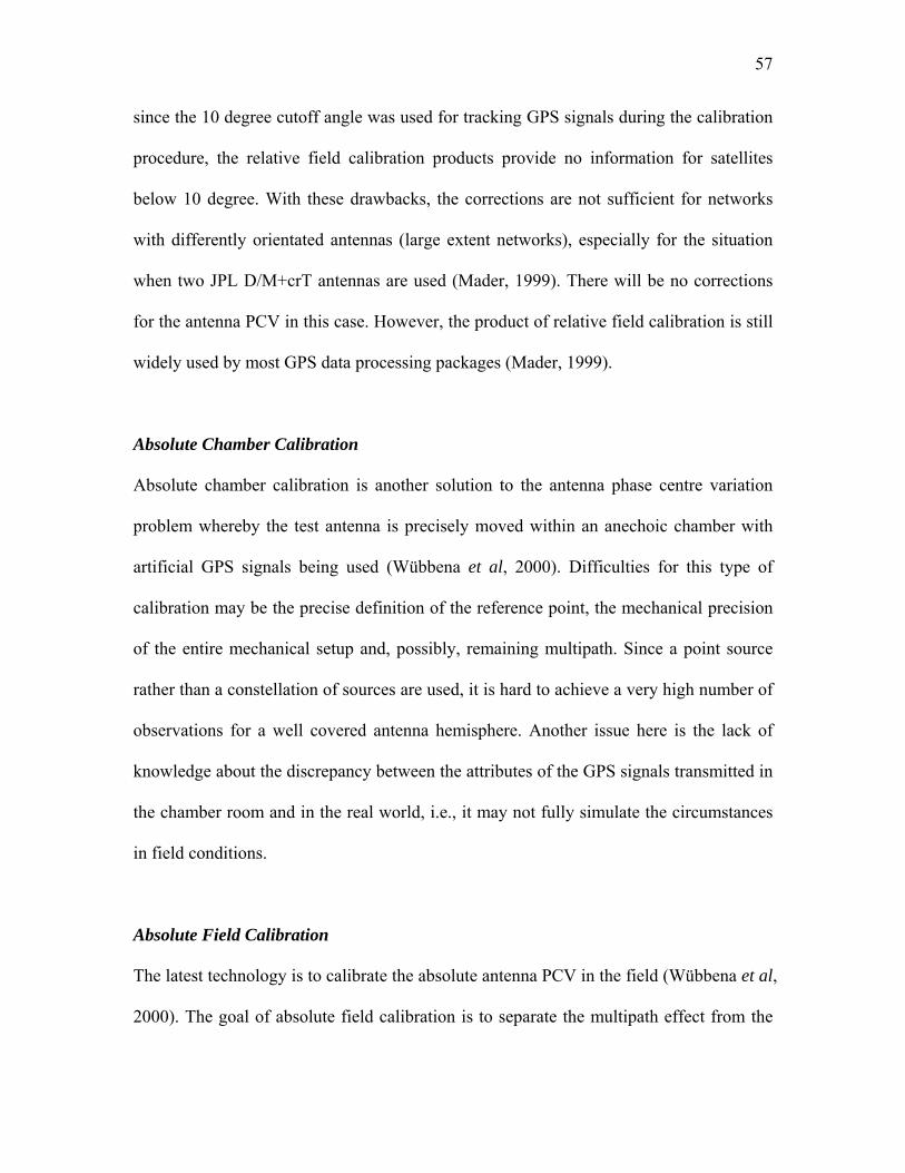
57

since the 10 degree cutoff angle was used for tracking GPS signals during the calibration

procedure, the relative field calibration products provide no information for satellites

below 10 degree. With these drawbacks, the corrections are not sufficient for networks

with differently orientated antennas (large extent networks), especially for the situation

when two JPL D/M+crT antennas are used (Mader, 1999). There will be no corrections

for the antenna PCV in this case. However, the product of relative field calibration is still

widely used by most GPS data processing packages (Mader, 1999).

Absolute Chamber Calibration

Absolute chamber calibration is another solution to the antenna phase centre variation

problem whereby the test antenna is precisely moved within an anechoic chamber with

artificial GPS signals being used (Wübbena et al, 2000). Difficulties for this type of

calibration may be the precise definition of the reference point, the mechanical precision

of the entire mechanical setup and, possibly, remaining multipath. Since a point source

rather than a constellation of sources are used, it is hard to achieve a very high number of

observations for a well covered antenna hemisphere. Another issue here is the lack of

knowledge about the discrepancy between the attributes of the GPS signals transmitted in

the chamber room and in the real world, i.e., it may not fully simulate the circumstances

in field conditions.

Absolute Field Calibration

The latest technology is to calibrate the absolute antenna PCV in the field (Wübbena et al,

2000). The goal of absolute field calibration is to separate the multipath effect from the

58

calibration results and to make it independent from a reference antenna and the test

station (location, satellite constellation in view on that station, etc.).

The realization is based on the use of a rotating antenna and the use of special

observation differences (i.e. sidereal Day difference). To achieve the rotation of the

antenna, an automatic precise robot was developed, which is able to rotate the antenna

around a fixed point (i.e. the nominal phase centre). The multipath effect is eliminated (in

fact greatly reduced) by post processing, making use of the property of multipath Day-to-

Day correlation. However, by sidereal Day difference, the antenna PCV was eliminated

in this procedure. The antenna PCV is re-introduced by rotation and tilt of the antenna.

The PCV difference between the no rotation/tilt on the reference Day and the rotation/tilt

on the second is used as input for PCV determination.

The rotation/tilt of the orientation of the antenna not only re-introduced the antenna PCV,

it also makes the coverage of the antenna’s hemisphere consistent and homogeneous even

with observations at the horizon. In this way, station dependencies were excluded. No

station dependence can be seen from the plot, like the northern hole and observations

down to elevation zero. Unfortunately, even with great advantage of this calibration

method, the product is not widely used.

4.1.2 Antenna PCV Experiment

Since only relative field antenna PCV calibration products are available at the processing

time, they are used in all the analysis carried out in this thesis. In order to evaluate the

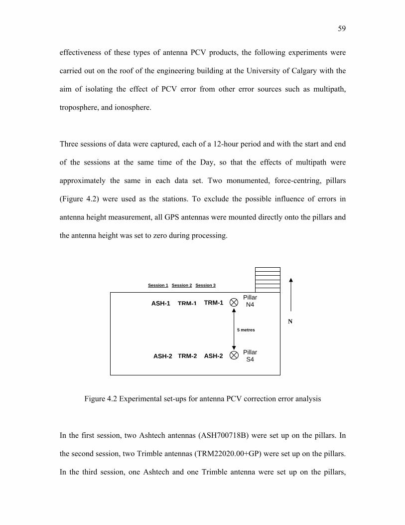
59

effectiveness of these types of antenna PCV products, the following experiments were

carried out on the roof of the engineering building at the University of Calgary with the

aim of isolating the effect of PCV error from other error sources such as multipath,

troposphere, and ionosphere.

Three sessions of data were captured, each of a 12-hour period and with the start and end

of the sessions at the same time of the Day, so that the effects of multipath were

approximately the same in each data set. Two monumented, force-centring, pillars

(Figure 4.2) were used as the stations. To exclude the possible influence of errors in

antenna height measurement, all GPS antennas were mounted directly onto the pillars and

the antenna height was set to zero during processing.

Session 1 Session 2 Session 3

Figure 4.2 Experimental set-ups for antenna PCV correction error analysis

In the first session, two Ashtech antennas (ASH700718B) were set up on the pillars. In

the second session, two Trimble antennas (TRM22020.00+GP) were set up on the pillars.

In the third session, one Ashtech and one Trimble antenna were set up on the pillars,

N

TRM-1

TRM-2

ASH-1 Pillar N4 TRM-1

5 metres

Pillar S4 ASH-2 ASH-2

60

respectively. The coordinates of pillar N4 were held fixed for all scenarios. In order to

investigate the impact of antenna PCV corrections on GPS positioning accuracy

(especially in height component) in different scenarios, the baselines were processed with

Bernese using both L1 and ionosphere-free (IF) frequency combinations with both

antenna PCV corrections on and off. The estimated station height difference between

pillar N4 and S4 in different scenarios were summarized in Table 4.1.

Even though in the case when the PCV corrections were switched off, the antenna PCV

error still can be cancelled out for this very short baseline when the same type of antenna

types were used. But if different types of antenna were used, the impact of antenna PCV

error becomes evident. In order to investigate the impact of PCV corrections, the

estimated station height difference between pillar N4 and S4 in different scenario were

compared as followed. As can be seen from Table 4.1, by switching the PCV corrections

on and off, the disagreement in relative height estimations for session 1 and session 2 of

1-2 mm (L1 solution compared with L1 solution, IF solution compared with IF solution).

When coming to the mixed antenna type scenario (session 3), the disagreement in relative

height estimations between the same type of solution when the PCV corrections switched

on and off of 6-20 mm.

Still the effectiveness of the relative field antenna PCV calibration products used in this

thesis is of interest. Therefore the relative height estimations between the scenarios when

PCV corrections switched on were compared as followed. The results given in Table 4.1

show a disagreement in relative height estimations between the scenarios of 1.4 mm to 12

61

mm with PCV corrections on. In the absence of other noise (the RMS of the residuals

was 3-4 mm in each case) this was assumed to stem from un-calibrated PCV effects,

especially in the mixed antenna case.

Table 4.1 Differences in height between pillars (m) estimated with three different antenna

configurations using L1 and IF processing strategies with both antenna PCV corrections

switched on and off

PCV corrections ON PCV corrections OFF

L1 IF L1 IF

Session 1 -0.0039 m -0.0027 m -0.0049 m -0.0025 m

Session 2 -0.0024 m -0.0059 m -0.0035 m -0.0075 m

Session 3 -0.0059 m -0.0144 m 0.0004 m -0.0335 m

The IF solution gives the biggest differences, which is in agreement with previous work

that shows this frequency combination to exacerbate the effects of an incorrect PCV

model (Wübbena et al, 2000). Although it does not make sense to process such a short

baseline with IF, the project baselines were all processed this way, and so the effects

were of interest. Since the baseline is so short, the ionospheric-free combination amplifies

noise without the benefit of removing ionospheric errors. The amplification of noise and

multipath for an IF solution compared to an L1 solution was given in Table 4.2.

62

Table 4.2 The amplification of noise and multipath for an IF solution compared to an L1

solution (Cannon and Lachapelle, 2003)

Error L1 Error (m) IF Error (m) Ratio 1

IFL

SV Position SVδρ∇∆ SVδρ∇∆ 1

Receiver Position recδρ∇∆ recδρ∇∆ 1

Troposphere tropδρ∇∆ tropδρ∇∆ 1

Ionosphere 21

1 ionof

− ∇∆ 0 0

Multipath m∇∆ 2 2

1 22

1 1

IF f fmf

λλ

+∇∆ 3.227

Noise ε∇∆ 2 2

1 22

1 1

IF f ff

λ ελ

+∇∆ 3.227

As can be seen from Table 4.1, with PCV corrections on, if an L1 solution is used, the

estimated station height differences between different antenna configurations are only

1.4-3 mm, which is near the level of the receiver noise. It can not really separate

uncorrected antenna PCV from receiver noise in this case. However, when looking at the

IF solution, the effect of mixed antennas is obvious. As can be seen, the difference

between the estimated station height difference between sessions 1 and 2, in which the

same type of antenna is used for each session but different types of antennas between

sessions, was only 3.3 mm. Since the same types of antennas were used, the uncorrected

antenna PCV can be cancelled out for this short baseline (5 m) in the double difference

processing like other error sources such as receiver clock offset, ionospheric delay, and

63

tropospheric delay. When it comes to the mixed antenna type scenario, the problem of

uncorrected antenna PCV is evident. The estimated station height differences between

sessions 1 and 3 and sessions 2 and 3 are 11.9 mm and 8.6 mm, respectively. It can be

concluded that the estimated station height error introduced by mixed antenna type in the

IF solution for this 5 m baseline was at 1 cm level. The main phase centre offset

component is vertical (up), which ranges from several centimetres to several tens of

centimetres, but there are also small horizontal offsets (north and east), which is generally

at millimetre level, that can be applied. There are actually two phase centres in an

antenna – one for the L1 frequency and the other for L2, and each phase centre has a

different offset.

4.2 Multipath

Multipath is another error source of interest, which can cause residuals of up to ¼ of the

GPS signal wavelength (approximately 5 cm on L1) (Ray, 2000). A brief introduction of

this type of error source can be found in Chapter 2, Section 2.4.4. There exist many

different methods for multipath identification and mitigation (see Section 2.4.4). In the

case of static GPS applications, multipath mitigation via Day-to-Day correlation can be

deemed as the most effective method. In this section, multipath mitigation via a Day-to-

Day correlation algorithm developed by Radovanovic (2000) was implemented and tested

under different conditions.

4.2.1 Multipath Mitigation via Day-To-Day Correlation Algorithm

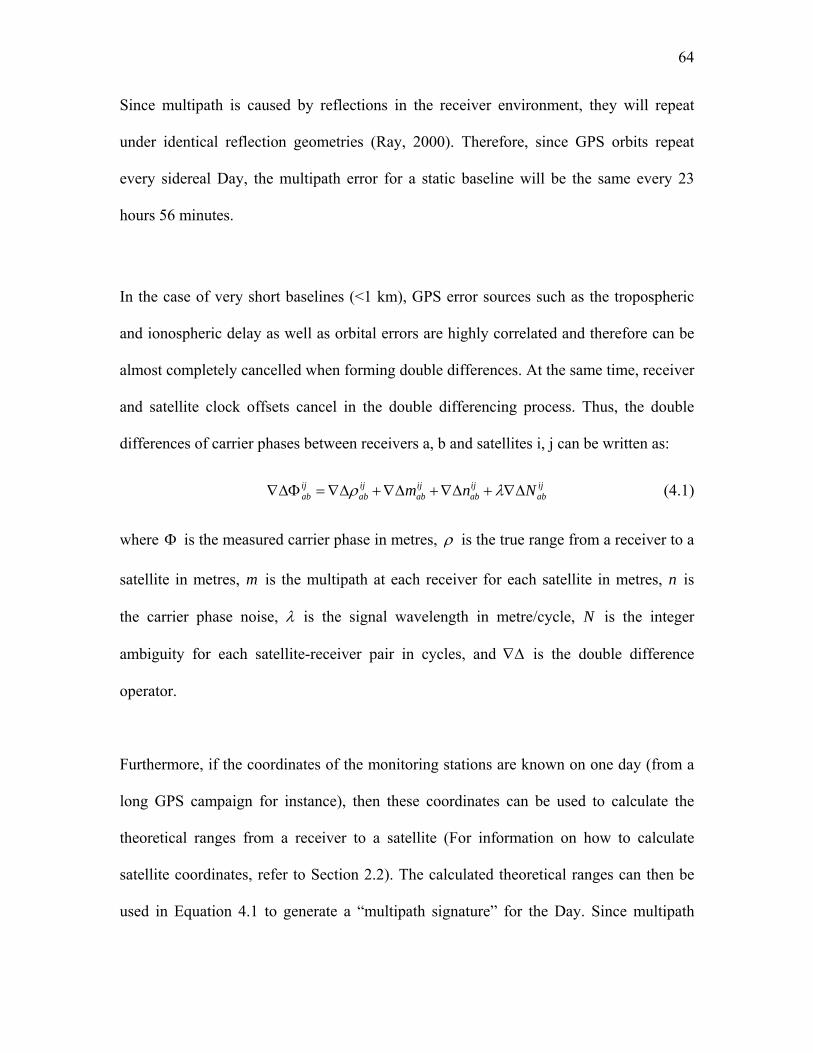
64

Since multipath is caused by reflections in the receiver environment, they will repeat

under identical reflection geometries (Ray, 2000). Therefore, since GPS orbits repeat

every sidereal Day, the multipath error for a static baseline will be the same every 23

hours 56 minutes.

In the case of very short baselines (<1 km), GPS error sources such as the tropospheric

and ionospheric delay as well as orbital errors are highly correlated and therefore can be

almost completely cancelled when forming double differences. At the same time, receiver

and satellite clock offsets cancel in the double differencing process. Thus, the double

differences of carrier phases between receivers a, b and satellites i, j can be written as:

(4.1) ij ij ij ij ijab ab ab ab abm nρ∇∆Φ = ∇∆ +∇∆ +∇∆ + ∇∆Nλ

where Φ is the measured carrier phase in metres, ρ is the true range from a receiver to a

satellite in metres, m is the multipath at each receiver for each satellite in metres, n is

the carrier phase noise, λ is the signal wavelength in metre/cycle, N is the integer

ambiguity for each satellite-receiver pair in cycles, and ∇∆ is the double difference

operator.

Furthermore, if the coordinates of the monitoring stations are known on one day (from a

long GPS campaign for instance), then these coordinates can be used to calculate the

theoretical ranges from a receiver to a satellite (For information on how to calculate

satellite coordinates, refer to Section 2.2). The calculated theoretical ranges can then be

used in Equation 4.1 to generate a “multipath signature” for the Day. Since multipath

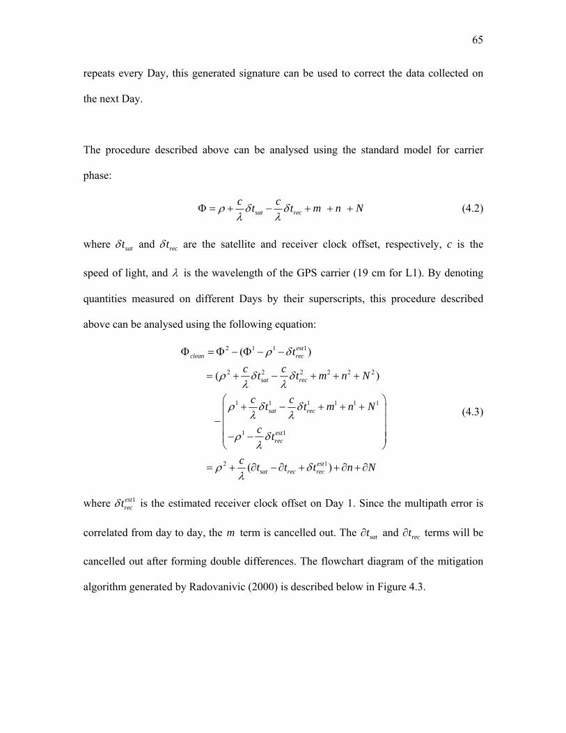
65

repeats every Day, this generated signature can be used to correct the data collected on

the next Day.

The procedure described above can be analysed using the standard model for carrier

phase:

sat recc ct t m nρ δ δλ λ

Φ = + − + + + N (4.2)

where sattδ and rectδ are the satellite and receiver clock offset, respectively, c is the

speed of light, and λ is the wavelength of the GPS carrier (19 cm for L1). By denoting

quantities measured on different Days by their superscripts, this procedure described

above can be analysed using the following equation:

2 1 1 1

2 2 2 2 2 2

1 1 1 1 1

1 1

2 1

( )

( )

( )

estclean rec

sat rec

sat rec

estrec

estsat rec rec

tc ct t m n N

c ct t m n N

c t

c t t t n N

ρ δ

ρ δ δλ λ

ρ δ δλ λ

ρ δλ

ρ δ

1

λ

Φ = Φ − Φ − −

= + − + + +

⎛ ⎞+ − + + +⎜− ⎜ ⎟⎜ ⎟− −⎜ ⎟⎝ ⎠

= + ∂ −∂ + + ∂ + ∂

⎟ (4.3)

where is the estimated receiver clock offset on Day 1. Since the multipath error is

correlated from day to day, the m term is cancelled out. The

1estrectδ

satt∂ and terms will be

cancelled out after forming double differences. The flowchart diagram of the mitigation

algorithm generated by Radovanivic (2000) is described below in Figure 4.3.

rect∂

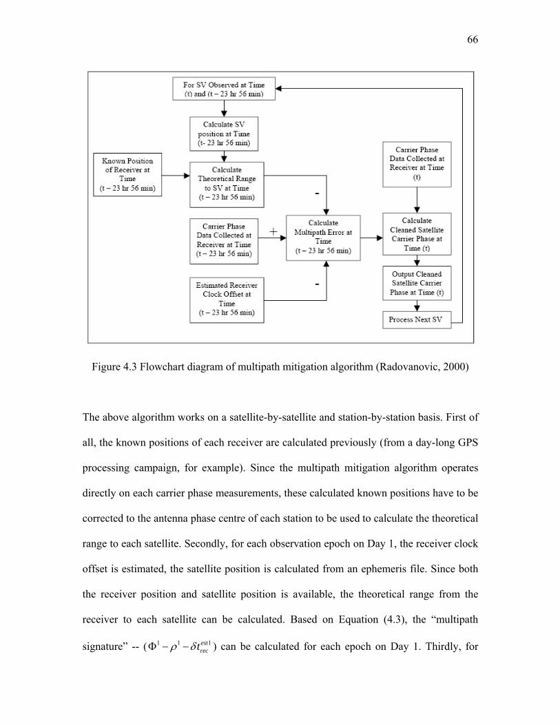
66

Figure 4.3 Flowchart diagram of multipath mitigation algorithm (Radovanovic, 2000)

The above algorithm works on a satellite-by-satellite and station-by-station basis. First of

all, the known positions of each receiver are calculated previously (from a day-long GPS

processing campaign, for example). Since the multipath mitigation algorithm operates

directly on each carrier phase measurements, these calculated known positions have to be

corrected to the antenna phase centre of each station to be used to calculate the theoretical

range to each satellite. Secondly, for each observation epoch on Day 1, the receiver clock

offset is estimated, the satellite position is calculated from an ephemeris file. Since both

the receiver position and satellite position is available, the theoretical range from the

receiver to each satellite can be calculated. Based on Equation (4.3), the “multipath

signature” -- ( ) can be calculated for each epoch on Day 1. Thirdly, for 1 1 estrectρ δΦ − − 1

67

each epoch on Day 2, the epoch time is deducted by 23 hr 56 min to locate the calculated

multipath signature on Day 1, which will be used to correct the carrier phase

measurement of the current epoch on Day 2. Fourthly, the cleaned carrier phase

measurements on Day 2 are output to a file with RINEX format. Finally, the above

described procedure is carried out on each epoch and each satellite.

The term is included such that the receiver clock offset of the cleaned observation

will be approximately the same as that of the Day two observation. In some GPS

receivers (such as the Ashtech Z-12), it allows the drift of the receiver clock error to grow

to 1 ms before resetting the clock. Figure 4.4 illustrates the drift properties of the receiver

clock of an Ashtech Z-12 receiver which was estimated through least squares batch

processing. If the term is not included, the clock jump information in the data on

Day 1 will remain in the cleaned phase observations after going through the procedures

described in Equation (4.3), which can cause problems for data processing with the

cleaned phase observation on Day 2. In this case, the clock jump information for Day 1

and Day 2 were mixed together, which will cause problem for the GPS software to detect

them. Again, this term will cancel out in a single difference between satellites.

1estrectδ

1estrectδ

68

Figure 4.4 Receiver clock drift for an Ashtech Z-12 receiver

The above described multipath mitigation algorithm has been implemented as a pre-

processor which operates on individual raw RINEX data files and outputs “clean” data in

RINEX format.

With the mitigation algorithm developed by Radovanovic (2000), some test results has

been reported. For his test results, the multipath mitigation algorithm can improve epoch-

by-epoch position accuracies from 25% to 40%. The improvement in accuracy mainly

depends on the magnitude of the multipath effect in the raw GPS data, i.e. for low

multipath environment, the multipath mitigation algorithm is less effective, while for

strong multipath environment, the effectiveness of the multipath mitigation algorithm is

evident. Moreover, if the data is first corrected using the multipath mitigation algorithm

and then the position estimates are averaged, the final accuracy improves by about 50%.

69

4.2.2 Test of the Mitigation Algorithm

In order to examine the success of the described algorithm, the following test procedures

were carried out on the roof of the engineering building at the University of Calgary. Two

Ashtech Z-12 receivers were mounted on pillars N1 and S1 separated by approximately 5

metres. About 12 hours of 15 s sampling interval dual-frequency data was collected at the

same time of Day at both stations.

The IGS station PRDS (approximately 25 km from the test site) was included here to

derive station coordinates for N1 and S1. By processing two 25 km baselines using all 12

hours worth of data in Bernese 4.2, the station coordinates for N1 and S1 were derived

and used as input as the reference coordinates in the multipath mitigation algorithm. After

the reference coordinates were derived, the test was then carried out on the 5-metre

baseline between N1 and S1. In later data processing, the coordinates of N1 were held

fixed to the derived reference coordinates and the station coordinates of S1 were to be

estimated.

Priori to testing the multipath mitigation algorithm, the repeatability of the multipath

error was examined. First, the station coordinates of N1 were held fixed to the above

derived reference coordinates and the station coordinates of S1 on Day 1 were estimated

on this 5-metre baseline. Then, the L1 fixed double difference residuals were generated

for both Days 1 and 2 by fixing the station coordinates of N1 and S1 to the estimated

station coordinates on Day 1. Figure 4.5 shows the DD residuals for the satellite pair

PRN1/11. As can be seen, the multipath errors are highly correlated between days. In all

70

the analysis carried out for multipath mitigation algorithm, the relative field antenna PCV

calibration products have been applied.

In order to better quantify the Day-to-Day correlation of multipath, the correlation

coefficients between two Day’s DD residuals were generated. The resulting plots for

satellite PRN1/11 are shown in Figure 4.6. The peak of the correlation coefficient (93%)

occurs with a 4 minute offset. Thus the correlation time of two consecutive Days is 23 hr

56 min (1 sidereal Day).

Figure 4.5 Two Day’s DD residuals generated by fixing both N1 and S1’s coordinates to

Day 1’s station coordinates estimation

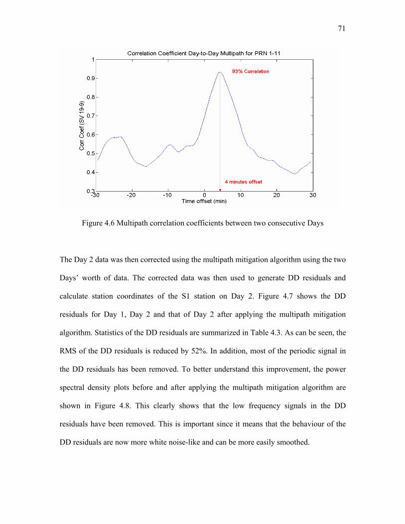
71

Figure 4.6 Multipath correlation coefficients between two consecutive Days

The Day 2 data was then corrected using the multipath mitigation algorithm using the two

Days’ worth of data. The corrected data was then used to generate DD residuals and

calculate station coordinates of the S1 station on Day 2. Figure 4.7 shows the DD

residuals for Day 1, Day 2 and that of Day 2 after applying the multipath mitigation

algorithm. Statistics of the DD residuals are summarized in Table 4.3. As can be seen, the

RMS of the DD residuals is reduced by 52%. In addition, most of the periodic signal in

the DD residuals has been removed. To better understand this improvement, the power

spectral density plots before and after applying the multipath mitigation algorithm are

shown in Figure 4.8. This clearly shows that the low frequency signals in the DD

residuals have been removed. This is important since it means that the behaviour of the

DD residuals are now more white noise-like and can be more easily smoothed.

72

Figure 4.7 DD residuals for Day 1, Day 2 and that of Day 2 after applying the multipath

mitigation algorithm

Table 4.3 Statistics of the DD residuals for Day 1, Day 2 and that of Day 2 after applying

the multipath mitigation algorithm

Day 1 Day 2 Day 2 corrected

Mean (mm) -0.6 -0.7 0.0

RMS (mm) 4.5 4.7 2.2

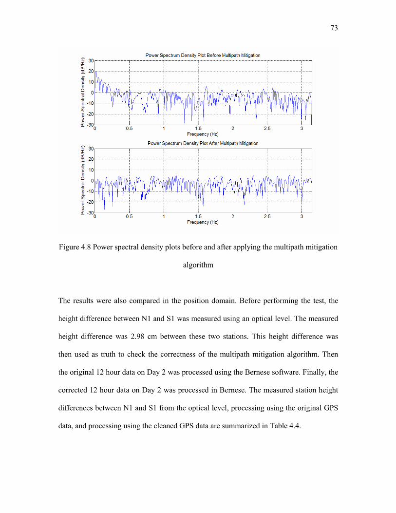
73

Figure 4.8 Power spectral density plots before and after applying the multipath mitigation

algorithm

The results were also compared in the position domain. Before performing the test, the

height difference between N1 and S1 was measured using an optical level. The measured

height difference was 2.98 cm between these two stations. This height difference was

then used as truth to check the correctness of the multipath mitigation algorithm. Then

the original 12 hour data on Day 2 was processed using the Bernese software. Finally, the

corrected 12 hour data on Day 2 was processed in Bernese. The measured station height

differences between N1 and S1 from the optical level, processing using the original GPS

data, and processing using the cleaned GPS data are summarized in Table 4.4.

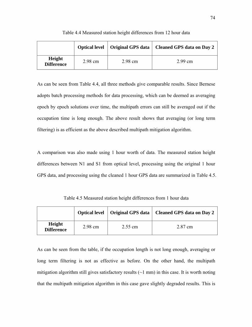
74

Table 4.4 Measured station height differences from 12 hour data

Optical level Original GPS data Cleaned GPS data on Day 2

Height Difference 2.98 cm 2.98 cm 2.99 cm

As can be seen from Table 4.4, all three methods give comparable results. Since Bernese

adopts batch processing methods for data processing, which can be deemed as averaging

epoch by epoch solutions over time, the multipath errors can still be averaged out if the

occupation time is long enough. The above result shows that averaging (or long term

filtering) is as efficient as the above described multipath mitigation algorithm.

A comparison was also made using 1 hour worth of data. The measured station height

differences between N1 and S1 from optical level, processing using the original 1 hour

GPS data, and processing using the cleaned 1 hour GPS data are summarized in Table 4.5.

Table 4.5 Measured station height differences from 1 hour data

Optical level Original GPS data Cleaned GPS data on Day 2

Height Difference 2.98 cm 2.55 cm 2.87 cm

As can be seen from the table, if the occupation length is not long enough, averaging or

long term filtering is not as effective as before. On the other hand, the multipath

mitigation algorithm still gives satisfactory results (~1 mm) in this case. It is worth noting

that the multipath mitigation algorithm in this case gave slightly degraded results. This is

75

because the satellite geometry starts to play its part in the results. It can be further

expected that this multipath mitigation algorithm can be even more effective for the

epoch-by-epoch solution case. Since this is not related to the work presented in this thesis,

this will not be discussed here.

76

CHAPTER 5

EXPERIMENTAL DESIGN AND DATA PROCESSING

Recent work in DGPS on the effects of location dependent variables such as satellite

geometry (Meng et al, 2004), tropospheric effects (Roberts and Rizos, 2004), and

ionospheric effects (Janssen et al, 2001) have mitigated these errors by employing an

optimised strategy for data capture and processing. The project described in this thesis

therefore investigated the location-dependent errors for this region, such as satellite

geometry, ionospheric effects, tropospheric effects and multipath, and the mitigation of

these errors through different field and processing approaches, based on the expectation

of an episodic campaign of DGPS measurements. Two GPS campaigns were carried out

in the target area to address these specific issues and precise levelling was used to gather

observations of the test points at a higher accuracy to provide ‘ground truth’ with which

to compare the DGPS results after data analysis and the application of different error

mitigation schemes. The aim of the project was to find the most accurate DGPS levelling

solution on baselines up to 130 km for this region.

This chapter first summarises the data collected in the summers of 2003 and 2004. A

study of the long term stability of different survey monument in permafrost was carried

out based on the analysis of two newly collected epochs of precise levelling data together

with historical data. GPS data processing was then carried out to investigate the impact of

different error sources on GPS height estimation for the target area. The repeatability

result analysis was used as an external assessment of the quality of the position results.

77

Based on the results, the best strategy for the field data collection and data processing

was developed and is presented at the end of the chapter.

5.1 Data Collection in summer 2003

In the summer of 2003, GPS data as well as precise levelling measurements were

collected at the Geodetic Survey of Canada (GSD) survey monument test-bed

(approximately 15 km from the INVK IGS station) in Inuvik, Northwest Territories to

establish the error budget for “GPS levelling” in the target area.

In 1987 the GSD established a long-term monitoring test-bed at the (then) Navy base in

Inuvik. The objective was to establish the stability of different types of survey

monuments in areas of continuous permafrost. The test-bed (Figure 5.1) comprised seven

different types of monuments (see Appendix 1 for a description of the monuments) in a

rough circle of diameter 70 metres, in an area described at the time as ‘wide open’. In

addition, benchmarks were placed in a link traverse along Navy Road to an area of

upland 3 km to the south of the test-bed. The monuments were measured by GSD using

differential levelling, twice a year (winter and summer campaigns) between summer 1987

and winter 1995, with a missing epoch in summer 1994. The measurements were then

discontinued.

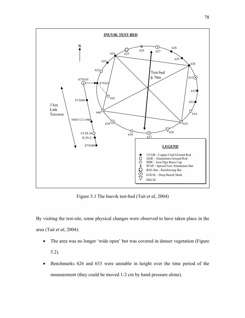
78

INUVIK TEST-BED

Figure 5.1 The Inuvik test-bed (Tait et al, 2004)

By visiting the test-site, some physical changes were observed to have taken place in the

area (Tait et al, 2004):

• The area was no longer ‘wide open’ but was covered in denser vegetation (Figure

5.2).

• Benchmarks 626 and 633 were unstable in height over the time period of the

measurement (they could be moved 1-2 cm by hand pressure alone).

XN 628 626 627

624 625

629 630

631

632

633

634

635

636 637

638

639

640

641

87T621

623

622 Test-bed φ 70m 87T610

87T609

87T608

NWT C3-1986

3 km Link Traverse

CCM-36 5L59-2-

LEGEND

CCGR - Copper Clad Ground Rod AGR - Aluminium Ground Rod IPBC - Iron Pipe Brass Cap SFAP - Spread Foot Aluminium Bar REE-Bar - Reinforcing Bar X

D.B.M. - Deep Bench Mark HELIX

79

• The benchmark at 608 had clearly been struck, presumably by earth-moving

equipment from the recent building in the immediate area. Other monuments on

the link traverse had been destroyed (CCM36, the cap had been sheared from this

steel pipe, presumably by snowplough) or were unstable (NWT C3-1986, a brass-

capped monument was in a swampy area by Navy Road and unstable during

measurement).

Four GPS receivers, including two Ashtech Z-12 GPS receivers with ASH700718B

antennas and two Trimble 4000SSI GPS receivers with TRM22020.00+GP antennas,

were used for data collection. All the GPS antennas were attached to a ground plane. The

equipment used at the INVK station was an Ashtech UZ-12 receiver connected with an

Ashtech 701945C_M choke ring antenna. Twenty-one monuments in this test-bed were

occupied during 6 sessions for 12 hours each with a sampling frequency of between 15-

30 seconds depending on the on-board memory of the receiver. The GPS data was

collected all using 5 degree cut-off angles. Three of the monuments were re-occupied for

similar periods of the day.

Observations of external accuracy were made of the relative heights of the stations using

differential levelling. The instrument used was a Leica 3003 digital level with a 3 m solid

Invar levelling rod. Misclosure of the circle observations was 0.05 mm, excluding 626

and 633 that could not be satisfactorily measured. Levelling the double-run between 610

and 621 gave a similar misclosure of 0.07 mm. The levelling result shows an order of

80

magnitude better precision than expected from DGPS levelling judged as being sufficient

to be used as ‘ground truth’ with which to compare the DGPS results.

Figure 5.2 Test-bed with a geodetic GPS receiver set over benchmark 623 (2004

campaign). Vegetation in the area was moderately-dense small trees and bushes, with

moss below.

5.2 Data Collection in summer 2004

In the summer 2004, another field campaign was carried out at the test site. Some

changes were made on the data collection scheme and are listed as follows:

1. Only Ashtech Z-12 receivers were used for the data collection for the 2004

campaign. Still, all the antennas were attached with a ground plane.

81

2. The GPS data was collected all using 0 degree cut-off angles and 30 sec sampling

intervals. The 0 degree cut-off angle was selected to allow the analysis of the

influence of different cut-off angles on height estimation. Since the sampling

interval used for the INVK station was 30 sec, only a 30 sec sampling interval for

data collection was needed. Based on the onboard memory size of the Ashtech Z-

12 receiver used, using a 30 sec sampling interval allows for the storage of 12

hours of data.

3. Data was collected on the same benchmark for the same period of time on two

consecutive days in order to allow for multipath mitigation via day-to-day

correlation analysis and repeatability analysis.

Applying the newly developed data collection scheme, new GPS data was collected at the

INVK test-bed through July 8 -15 and July 24 - 27, 2004. Levelling measurements were

made using an optical level (NA2) as an external check for the GPS height estimation.

Table 5.1 summarizes the 2003 and 2004 DGPS campaigns and external data collection.

82

Table 5.1 Summary of 2003 / 2004 DGPS campaign and external data collection

Length (km)

Rover type (s)

Choke

ring

# of stations occupied

Occupation length (h) / sampling

frequency (s)

# re-occupied

External comparison

15 (2003)

Ashtech Z12

Trimble 4000SSI

N 21 12 / 15-30 3

Differential levelling

(Reduced level estimated accuracy

0.02mm 1σ)

15 (2004)

Ashtech Z12 N 6 (twice) 12 / 30 6 (twice)

Differential levelling

(RL 1.1mm 1σ)

130 Ashtech UZ12 Y 2

12 / 30

(Data from CDDIS)

N/A IGS weekly

average coordinates

5.3 Long-term Stability of Different Survey Monument in Permafrost

Since it was desirable to have both vertical and planimetric measurements of deformation,

a monumented solution using DGPS observations was recommended (Tait and Moorman,

2003). However, this method relies on the measurement station to remain stable for 20-30

years. A stability study of seven different types of monuments had been carried out at the

Inuvik test-bed (see Section 5.1 for a full description of the Inuvik test-bed).

In the summers of 2003 and 2004, two new epochs of GPS and precise levelling

observations were made. These newly collected height difference measurements, together

with the historical data (height difference measurements collected from 1987 to 1995)

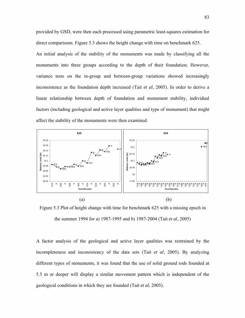
83

provided by GSD, were then each processed using parametric least-squares estimation for

direct comparisons. Figure 5.3 shows the height change with time on benchmark 625.

An initial analysis of the stability of the monuments was made by classifying all the

monuments into three groups according to the depth of their foundation. However,

variance tests on the in-group and between-group variations showed increasingly

inconsistence as the foundation depth increased (Tait et al, 2005). In order to derive a

linear relationship between depth of foundation and monument stability, individual

factors (including geological and active layer qualities and type of monument) that might

affect the stability of the monuments were then examined.

625

87Sw

88Sw 89S

w90S

w91S

w92S

w93S

ww

18.02

18.04

18.06

18.08

18.1

18.12

18.14

18.16

18.18

87S

w 88S

w 89S

w 90S

w 91S

w 92S

w 93S

w 94S

w

Year/Season

Red

uce

Leve

l (m

)

625

87Sw 88Sw 89Sw 90Sw 91S

w92S

w 93Sw

w

03S04S

17.95

18

18.05

18.1

18.15

18.2

18.25

87Sw 88Sw 89Sw 90Sw 91Sw 92Sw 93Sw 94Sw 95Sw 96Sw 97Sw 98Sw 99Sw 00Sw 01Sw 02Sw 03Sw 04S

Year/Season

Red

uce

Leve

l (m

)

(a) (b)

Figure 5.3 Plot of height change with time for benchmark 625 with a missing epoch in

the summer 1994 for a) 1987-1995 and b) 1987-2004 (Tait et al, 2005)

A factor analysis of the geological and active layer qualities was restrained by the

incompleteness and inconsistency of the data sets (Tait et al, 2005). By analyzing

different types of monuments, it was found that the use of solid ground rods founded at

5.5 m or deeper will display a similar movement pattern which is independent of the

geological conditions in which they are founded (Tait et al, 2005).

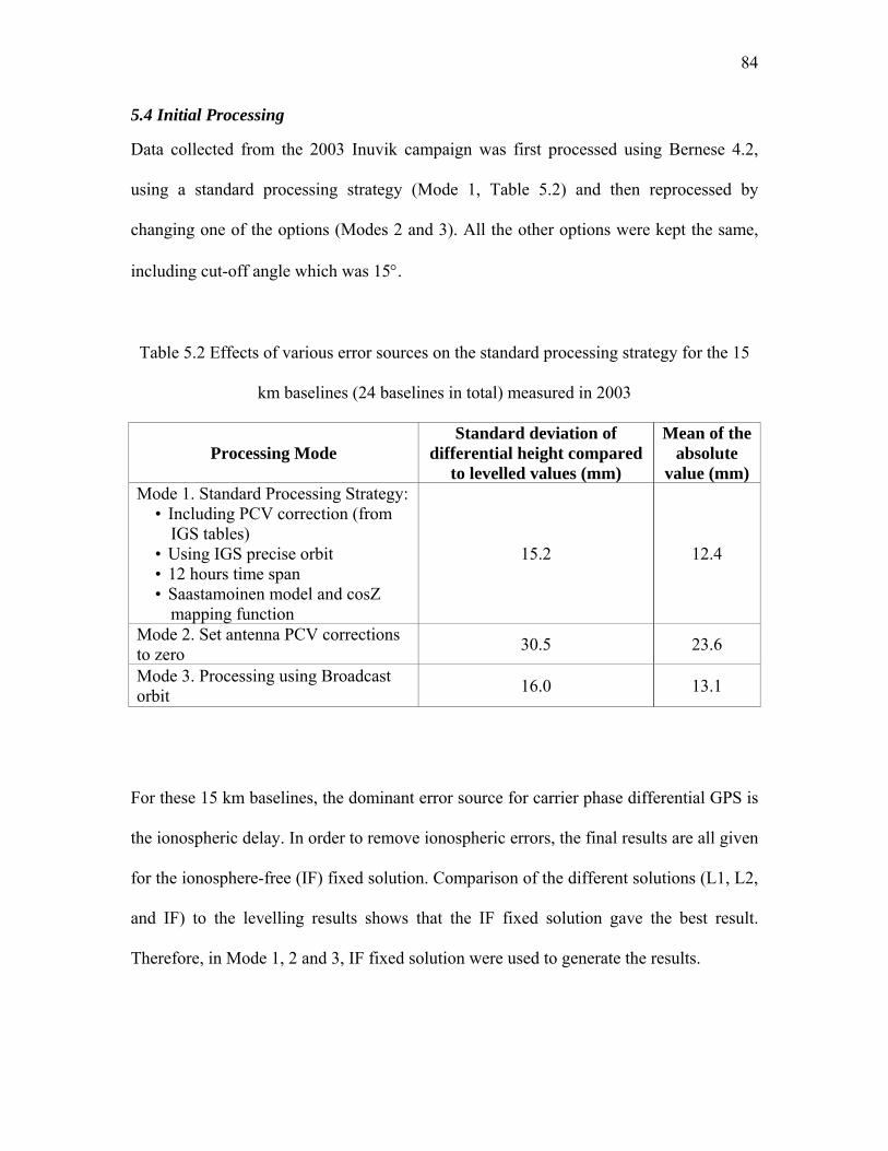
84

5.4 Initial Processing

Data collected from the 2003 Inuvik campaign was first processed using Bernese 4.2,

using a standard processing strategy (Mode 1, Table 5.2) and then reprocessed by

changing one of the options (Modes 2 and 3). All the other options were kept the same,

including cut-off angle which was 15°.

Table 5.2 Effects of various error sources on the standard processing strategy for the 15

km baselines (24 baselines in total) measured in 2003

Processing Mode Standard deviation of

differential height compared to levelled values (mm)

Mean of the absolute

value (mm) Mode 1. Standard Processing Strategy:

• Including PCV correction (from IGS tables)

• Using IGS precise orbit • 12 hours time span • Saastamoinen model and cosZ

mapping function

15.2 12.4

Mode 2. Set antenna PCV corrections to zero 30.5 23.6

Mode 3. Processing using Broadcast orbit 16.0 13.1

For these 15 km baselines, the dominant error source for carrier phase differential GPS is

the ionospheric delay. In order to remove ionospheric errors, the final results are all given

for the ionosphere-free (IF) fixed solution. Comparison of the different solutions (L1, L2,

and IF) to the levelling results shows that the IF fixed solution gave the best result.

Therefore, in Mode 1, 2 and 3, IF fixed solution were used to generate the results.

85

Since the precise levelling measurements are given in station height differences, the

estimated station heights from GPS data were then used to calculate station height

differences in order to compare the result with precise levelling directly. The standard

deviation of the differences between GPS derived height differences and levelled values

are calculated and listed in Table 5.2. The mean value of the absolute value of above

mentioned differences are also calculated.

The mean value is not calculated directly here because it does not give any information

on the “GPS levelling” accuracy. Since all the benchmark forms were aligned on a circle,

the sum of the height difference is actually the “GPS levelling” misclosure on the circle,

which is very close to zero.

As can be seen from Table 5.2, the effect of PCV correction is significant as expected,

and errors using broadcast orbital ephemeris display the insignificant affect anticipated in

theory.

5.5 Antenna Phase Centre Variation

In the 2003 GPS campaign, three benchmarks on the test-site were re-occupied with a

different antenna (Trimble TRM22020.00+GP and Ashtech 700718 antennas), as well as

with the same type. On examination of the repeatability of the station height estimation,

those stations occupied by the same types of antenna gave agreement within 2 mm, while

the stations occupied by the different types of antenna was around 3 cm (see Table 5.3).

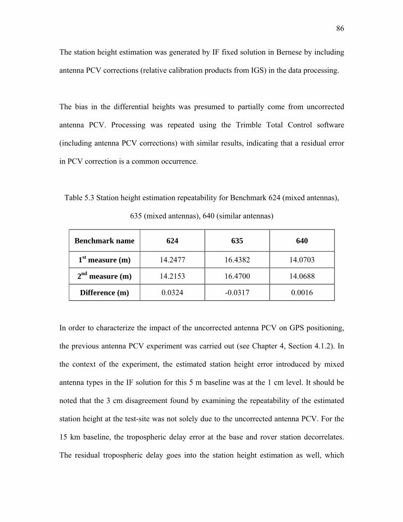
86

The station height estimation was generated by IF fixed solution in Bernese by including

antenna PCV corrections (relative calibration products from IGS) in the data processing.

The bias in the differential heights was presumed to partially come from uncorrected

antenna PCV. Processing was repeated using the Trimble Total Control software

(including antenna PCV corrections) with similar results, indicating that a residual error

in PCV correction is a common occurrence.

Table 5.3 Station height estimation repeatability for Benchmark 624 (mixed antennas),

635 (mixed antennas), 640 (similar antennas)

Benchmark name 624 635 640

1st measure (m) 14.2477 16.4382 14.0703

2nd measure (m) 14.2153 16.4700 14.0688

Difference (m) 0.0324 -0.0317 0.0016

In order to characterize the impact of the uncorrected antenna PCV on GPS positioning,

the previous antenna PCV experiment was carried out (see Chapter 4, Section 4.1.2). In

the context of the experiment, the estimated station height error introduced by mixed

antenna types in the IF solution for this 5 m baseline was at the 1 cm level. It should be

noted that the 3 cm disagreement found by examining the repeatability of the estimated

station height at the test-site was not solely due to the uncorrected antenna PCV. For the

15 km baseline, the tropospheric delay error at the base and rover station decorrelates.

The residual tropospheric delay goes into the station height estimation as well, which

87

contributes to the 3 cm disagreement. In addition, only two types of antennas

(TRM22020.00+GP and ASH700718) were used in the antenna PCV experiment carried

out on the roof of the engineering building, while three types of antenna

(TRM22020.00+GP, ASH700718, and ASH701945C_M) were involved in the 2003

summer field campaign. In this case, the uncorrected antenna PCV for the

ASH701945C_M antenna may have magnified the impact of the antenna PCV on

positioning accuracy.

Based on the above analysis, only one type of receiver/antenna was used for the 2004

summer campaign in order to avoid the potential problem arising by the use of mixed

antenna types.

5.6 Ionosphere and Satellite Geometry

5.6.1 Influence of Enhanced Ionospheric Activities on GPS Receiver Tracking

Performance

The target area lies within the auroral region (Figure 5.4). The auroral region is typically

located between 65 and 75º, where the visible aurora occurs overhead (Rostoker and

Skone, 1993). These regions are characterised by enhanced energetic electron

precipitation (Skone, 2001). The associated irregularities in electron density lead to rapid

phase and amplitude fluctuations when GPS signal travel through the ionosphere, known

as scintillation effects (Skone, 2001).

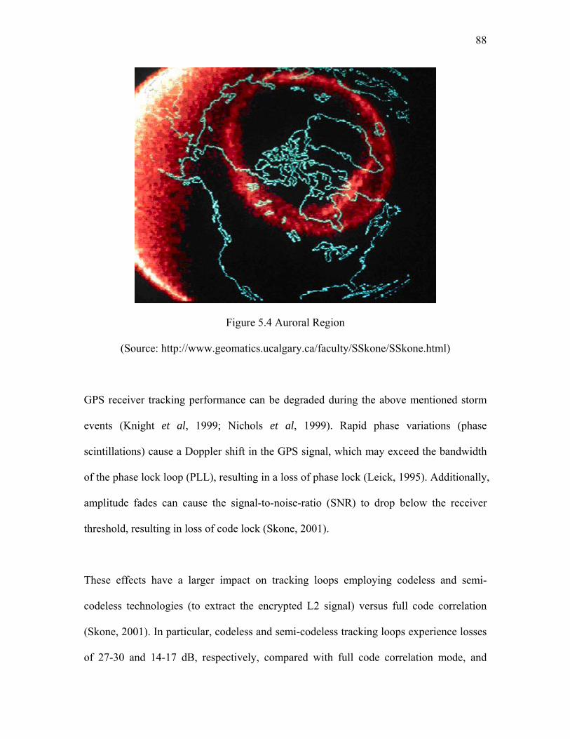
88

Figure 5.4 Auroral Region

(Source: http://www.geomatics.ucalgary.ca/faculty/SSkone/SSkone.html)

GPS receiver tracking performance can be degraded during the above mentioned storm

events (Knight et al, 1999; Nichols et al, 1999). Rapid phase variations (phase

scintillations) cause a Doppler shift in the GPS signal, which may exceed the bandwidth

of the phase lock loop (PLL), resulting in a loss of phase lock (Leick, 1995). Additionally,

amplitude fades can cause the signal-to-noise-ratio (SNR) to drop below the receiver

threshold, resulting in loss of code lock (Skone, 2001).

These effects have a larger impact on tracking loops employing codeless and semi-

codeless technologies (to extract the encrypted L2 signal) versus full code correlation

(Skone, 2001). In particular, codeless and semi-codeless tracking loops experience losses

of 27-30 and 14-17 dB, respectively, compared with full code correlation mode, and

89

therefore are more susceptible to the effects of amplitude fading (Cannon and Lachapelle,

2003). Availability of the L2 signal is particularly important for positioning applications

requiring the formation of ionosphere-free combination.

The receiver performance can be quantified in terms of both the number of cycle slips

detected and the number of observations missing during reacquisition periods. It is

necessary to consider the number of missing observations as an additional statistic in

order to accurately reflect the range of the receiver performance (Skone, 2001). When

loss of tracking happens, a reacquisition period is required for the receiver to re-track the

GPS signal. During this time period, observations may be missing during data dropouts.

The longer the reacquisition periods needed for receivers, the more observations will be

missing. In such cases only one cycle slip will be detected, but the impact on positioning

applications is significant in terms of data dropouts (Skone, 2001).

Table 5.4 shows the marked unpaired L1/L2 observations and cycle slips reported from

Bernese for the GPS data collected in 2003. As can be observed in Table 5.4, the Ashtech

Z-12 receiver has a better performance than the Trimble 4000SSI receiver. The tracking

loop of the Ashtech Z-12 receiver employs semi-codeless technology, while the tracking

loop of the Trimble 4000SSI receiver employs codeless technology (Skone and de Jong,

2000). The performance of these two types of receiver coincides with the aforementioned

conclusion. The performance of the L1 tracking loop is better than the L2 tracking loop,

since the L1 tracking loop employs full code correlation technology, in which case no

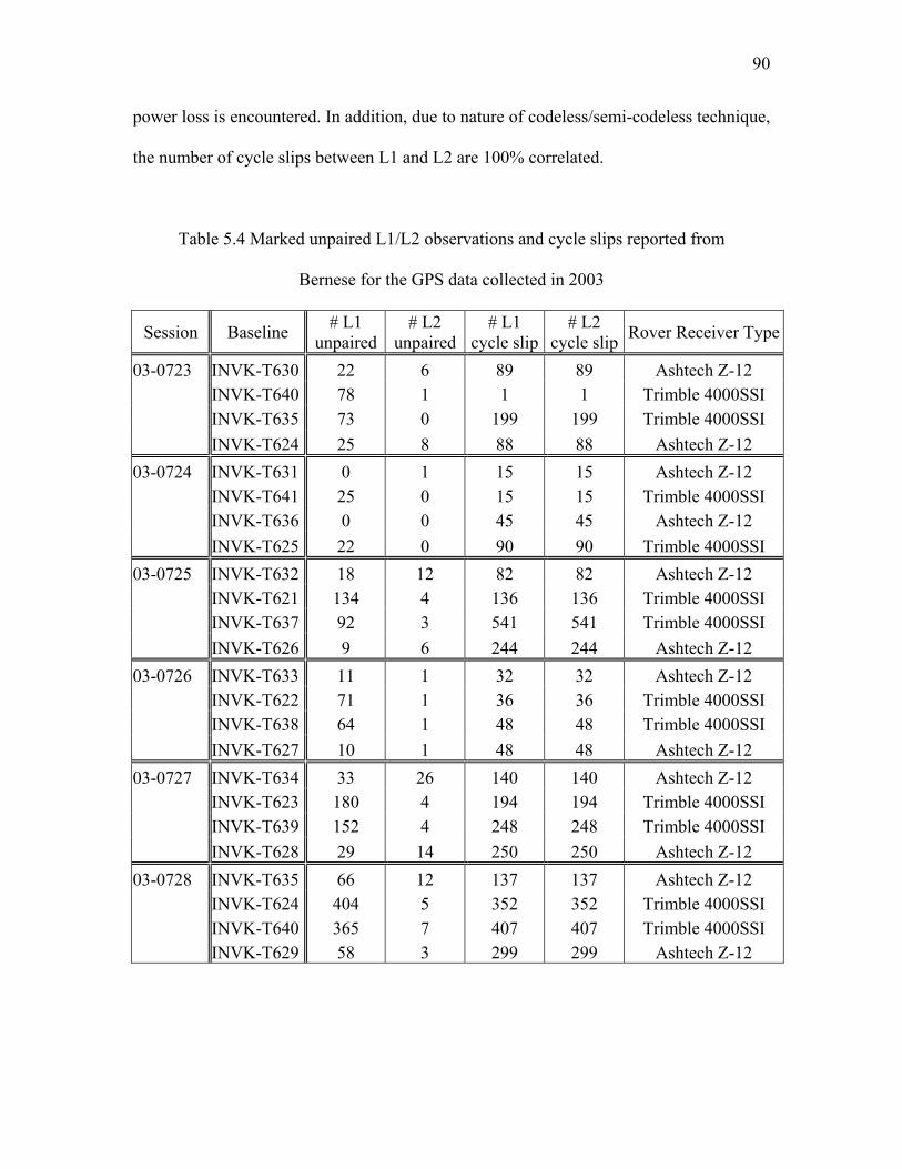
90

power loss is encountered. In addition, due to nature of codeless/semi-codeless technique,

the number of cycle slips between L1 and L2 are 100% correlated.

Table 5.4 Marked unpaired L1/L2 observations and cycle slips reported from

Bernese for the GPS data collected in 2003

Session Baseline # L1 unpaired

# L2 unpaired

# L1 cycle slip

# L2 cycle slip Rover Receiver Type

03-0723 INVK-T630 22 6 89 89 Ashtech Z-12 INVK-T640 78 1 1 1 Trimble 4000SSI INVK-T635 73 0 199 199 Trimble 4000SSI INVK-T624 25 8 88 88 Ashtech Z-12 03-0724 INVK-T631 0 1 15 15 Ashtech Z-12 INVK-T641 25 0 15 15 Trimble 4000SSI INVK-T636 0 0 45 45 Ashtech Z-12 INVK-T625 22 0 90 90 Trimble 4000SSI 03-0725 INVK-T632 18 12 82 82 Ashtech Z-12 INVK-T621 134 4 136 136 Trimble 4000SSI INVK-T637 92 3 541 541 Trimble 4000SSI INVK-T626 9 6 244 244 Ashtech Z-12 03-0726 INVK-T633 11 1 32 32 Ashtech Z-12 INVK-T622 71 1 36 36 Trimble 4000SSI INVK-T638 64 1 48 48 Trimble 4000SSI INVK-T627 10 1 48 48 Ashtech Z-12 03-0727 INVK-T634 33 26 140 140 Ashtech Z-12 INVK-T623 180 4 194 194 Trimble 4000SSI INVK-T639 152 4 248 248 Trimble 4000SSI INVK-T628 29 14 250 250 Ashtech Z-12 03-0728 INVK-T635 66 12 137 137 Ashtech Z-12 INVK-T624 404 5 352 352 Trimble 4000SSI INVK-T640 365 7 407 407 Trimble 4000SSI INVK-T629 58 3 299 299 Ashtech Z-12

91

Most of the cycle slips reported by Bernese were actually due to the resetting of the

receiver clock. In some GPS receivers, it allows the receiver clock offset to grow to 1 ms

before resetting the clock (see Section 4.2.1). This kind of property depends on the

receiver design.

By examine the Kp index for each session listed in Table 5.4, enhanced ionospheric

activities was experienced (Kp > 4) during the data collection of session 03-0725, 03-

0727, and 03-0728. Correspondingly, more unpaired L1 and L2 observations (especially

unpaired L1 observations) were reported in Table 5.4 for these three sessions. This

impact is more obvious on Trimble 4000SSI receivers, which adopt codeless tracking

technique.

For the above mentioned reason, only the Ashtech Z-12 receivers adopting semi-codeless

tracking technique were used in the 2004 campaign. The use of semi-codeless receivers

for the 2004 15 km and 130 km baselines gave approximately 30-40 cycle-slips per 12-

hour session at 15° elevations. These data were used in all the following analyses.

5.6.2 Influence of Enhanced Ionospheric Activities on GPS Positioning Accuracy

This section examines whether or not the most effective processing of the baselines

observed using the IF solution, together with the usual Elevation Dependent Weighting

(EDW) measures associated with path delay correction, are effective during an

ionospheric event. The balance between reducing errors in longer paths and maintaining

the best satellite geometry was also of interest.

92

In order to assess the most appropriate strategy for processing data observed during an

ionospheric event, two 15 km baselines were chosen from the 2004 campaign that each

had 12-hour observations in both a quiet ionospheric period and during an ionospheric

event. These periods were assessed using the one-minute variation of geomagnetic field

for the Yellowknife station, the closest station to the test area (approximately 1100 km).

The dates chosen were July 14 and 25, the assessments of which are shown in Figures

5.5a and 5.5b.

(a)

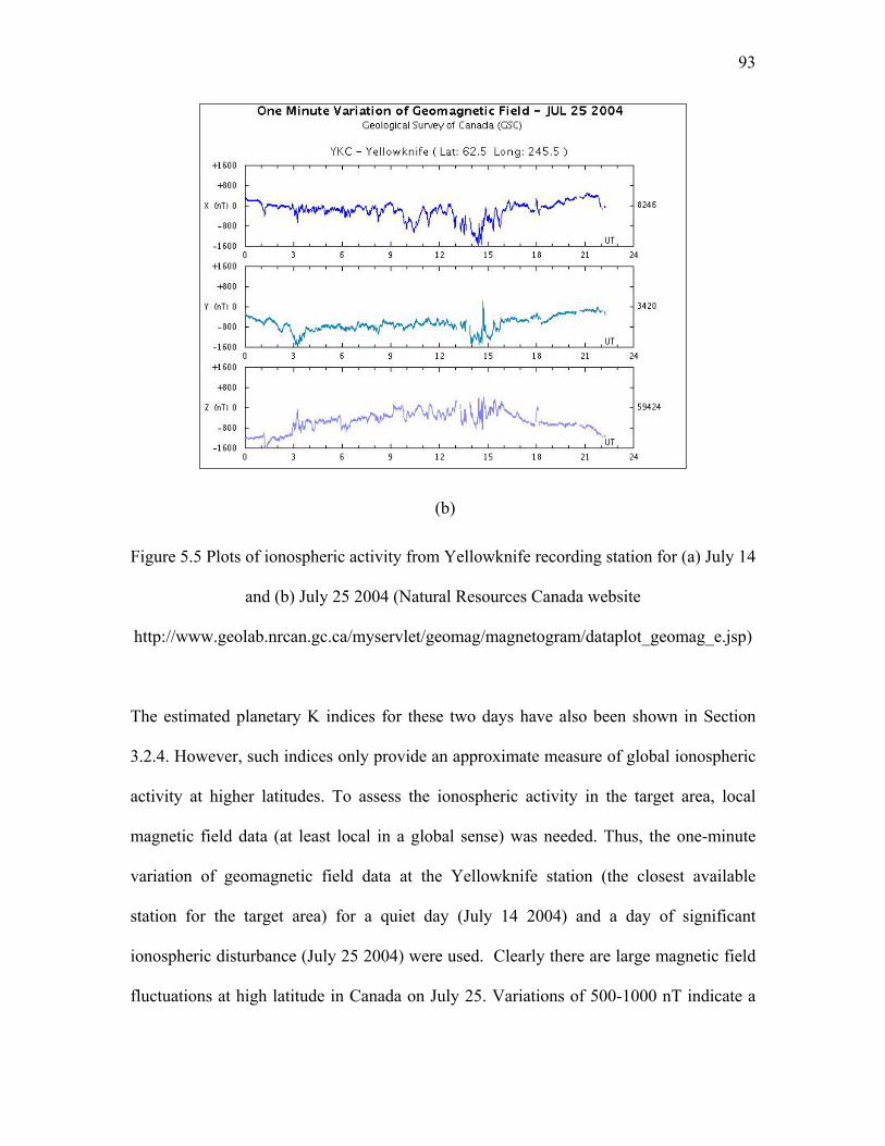
93

(b)

Figure 5.5 Plots of ionospheric activity from Yellowknife recording station for (a) July 14

and (b) July 25 2004 (Natural Resources Canada website

http://www.geolab.nrcan.gc.ca/myservlet/geomag/magnetogram/dataplot_geomag_e.jsp)

The estimated planetary K indices for these two days have also been shown in Section

3.2.4. However, such indices only provide an approximate measure of global ionospheric

activity at higher latitudes. To assess the ionospheric activity in the target area, local

magnetic field data (at least local in a global sense) was needed. Thus, the one-minute

variation of geomagnetic field data at the Yellowknife station (the closest available

station for the target area) for a quiet day (July 14 2004) and a day of significant

ionospheric disturbance (July 25 2004) were used. Clearly there are large magnetic field

fluctuations at high latitude in Canada on July 25. Variations of 500-1000 nT indicate a

94

storm event. An event of such magnitude has a frequency of approximately 10-12 times

per year and duration of around 24 hours (Skone, 2003).

The baselines were processed at different cut-off angles to determine whether there was a

‘best’ configuration of processing in these conditions. The 2004 15 km baselines were

processed for both days with EDW both activated and switched off. The results

demonstrated no major advantages gained through the application of EDW during the

July 14 dataset, and a worsening of the result using EDW during the 25 July session. In

terms of path length versus geometry, external accuracy assessments displayed an

increasing accuracy from 0° until the 15° cut-off was reached, followed by a reduction in

accuracy. In the longer baselines (130 km), with larger expected differences in

atmospheric delays at the stations, the same trend was evident (Table 5.5).

Table 5.5 Effect of the variation in cut-off angle, and the use of the EDW, for two 130

km baselines observed on July 14 and July 25 2004. Estimates of height and the mean

and standard deviations between these and weekly IGS averages results are shown.

Estimated heights (GPS) in metres 12 hour session height TUKT–

weekly average (m) Cut-off angle

(degrees) July 14

EDW on

July 14

EDW off

July 25

EDW on

July 25

EDW offmean 1σ

0 -1.5313 -1.5348 -1.5440 -1.5357 -0.0074 0.0070 5 -1.5461 -1.5363 -1.5494 -1.5357 -0.0129 0.0074 10 -1.5415 -1.5339 -1.5358 -1.5299 -0.0063 0.0040 15 -1.5321 -1.5283 -1.5249 -1.5253 0.0014 0.0018

95

20 -1.5228 -1.5220 -1.5233 -1.5230 0.0062 0.0025 Average height

estimated -1.5348 -1.5311 -1.5355 -1.5300

Note: IGS height difference = -1.5308m for July 14 and -1.5272m for July 25

5.7 Tropospheric Delay Estimation Strategy

When processing GPS data, the tropospheric delay is typically predicted using empirical

models, such as models developed by Saastamoinen (1972) and Hopfield (1970). By

using these models, standard or measured ground meteorological data, such as

temperature, pressure and humidity, must be provided. However, even when accurate

meteorological data is available, the predicted tropospheric delay from these models still

does not have a high accuracy. The residual tropospheric delay can be the largest

remaining error source in dual-frequency precision positioning (Collins and Langley,

1997).

Since tropospheric delay is a spatially dependent error source, it can not be completely

removed by forming double differencing for long baselines. The differential tropospheric

delay may be significant depending on the meteorological conditions in base and rover

stations (ranging from 1-3 ppm in extreme conditions). Yunck (1993) pointed out that the

tropospheric delay error in the vertical component far exceeds the inherent geometric

weakness of GPS.

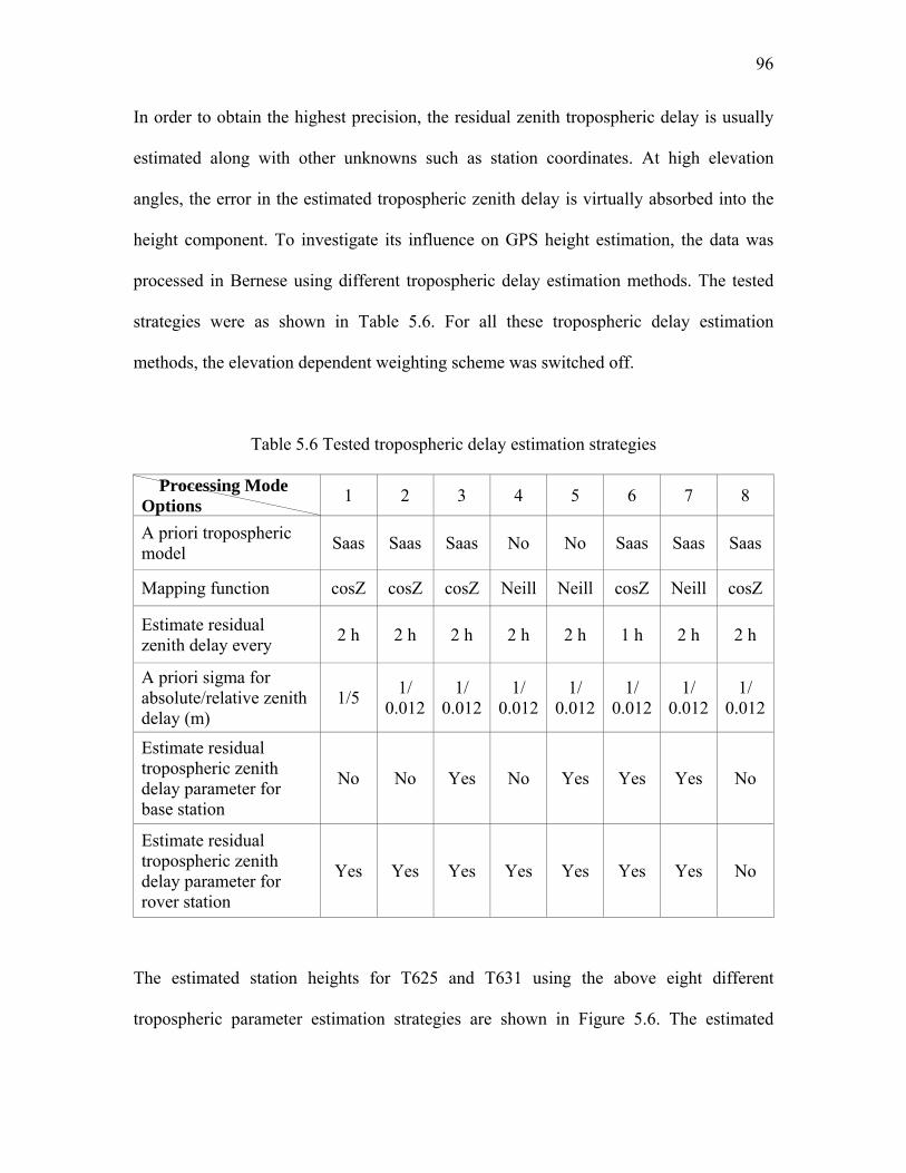
96

In order to obtain the highest precision, the residual zenith tropospheric delay is usually

estimated along with other unknowns such as station coordinates. At high elevation

angles, the error in the estimated tropospheric zenith delay is virtually absorbed into the

height component. To investigate its influence on GPS height estimation, the data was

processed in Bernese using different tropospheric delay estimation methods. The tested

strategies were as shown in Table 5.6. For all these tropospheric delay estimation

methods, the elevation dependent weighting scheme was switched off.

Table 5.6 Tested tropospheric delay estimation strategies

Processing Mode Options 1 2 3 4 5 6 7 8

A priori tropospheric model Saas Saas Saas No No Saas Saas Saas

Mapping function cosZ cosZ cosZ Neill Neill cosZ Neill cosZ

Estimate residual zenith delay every 2 h 2 h 2 h 2 h 2 h 1 h 2 h 2 h

A priori sigma for absolute/relative zenith delay (m)

1/5 1/ 0.012

1/ 0.012

1/ 0.012

1/ 0.012

1/ 0.012

1/ 0.012

1/ 0.012

Estimate residual tropospheric zenith delay parameter for base station

No No Yes No Yes Yes Yes No

Estimate residual tropospheric zenith delay parameter for rover station

Yes Yes Yes Yes Yes Yes Yes No

The estimated station heights for T625 and T631 using the above eight different

tropospheric parameter estimation strategies are shown in Figure 5.6. The estimated

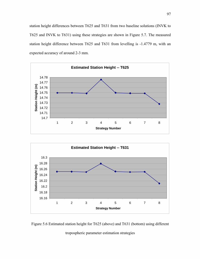
97

station height differences between T625 and T631 from two baseline solutions (INVK to

T625 and INVK to T631) using these strategies are shown in Figure 5.7. The measured

station height difference between T625 and T631 from levelling is -1.4779 m, with an

expected accuracy of around 2-3 mm.

Estimated Station Height -- T625

14.714.7114.7214.7314.7414.7514.7614.7714.78

1 2 3 4 5 6 7 8

Strategy Number

Stat

ion

Hei

ght (

m)

Estimated Station Height -- T631

16.16

16.18

16.2

16.22

16.24

16.26

16.28

16.3

1 2 3 4 5 6 7 8

Strategy Number

Stat

ion

Hei

ght (

m)

Figure 5.6 Estimated station height for T625 (above) and T631 (bottom) using different

tropospheric parameter estimation strategies

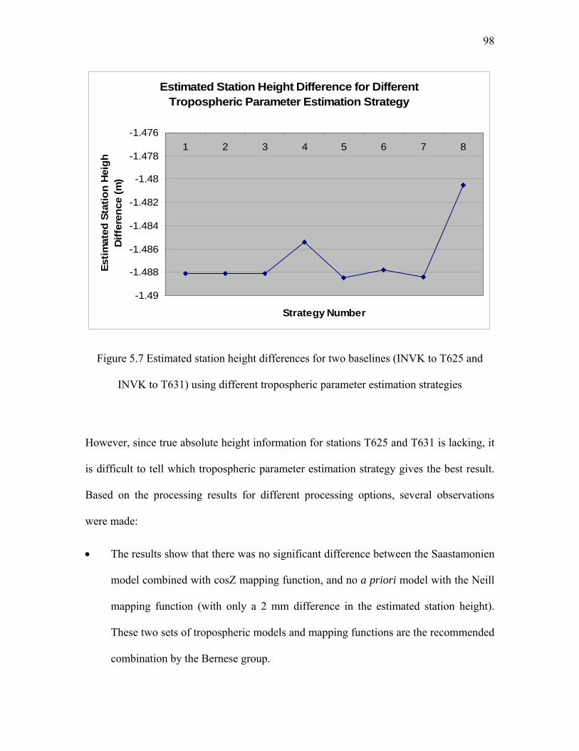
98

Estimated Station Height Difference for Different Tropospheric Parameter Estimation Strategy

-1.49

-1.488

-1.486

-1.484

-1.482

-1.48

-1.478

-1.4761 2 3 4 5 6 7 8

Strategy Number

Estim

ated

Sta

tion

Hei

ghD

iffer

ence

(m)

Figure 5.7 Estimated station height differences for two baselines (INVK to T625 and

INVK to T631) using different tropospheric parameter estimation strategies

However, since true absolute height information for stations T625 and T631 is lacking, it

is difficult to tell which tropospheric parameter estimation strategy gives the best result.

Based on the processing results for different processing options, several observations

were made:

• The results show that there was no significant difference between the Saastamonien

model combined with cosZ mapping function, and no a priori model with the Neill

mapping function (with only a 2 mm difference in the estimated station height).

These two sets of tropospheric models and mapping functions are the recommended

combination by the Bernese group.

99

• The a priori sigma value for absolute zenith delay constrains individual

tropospheric parameters to the a priori model value. While the a priori sigma value

for the relative zenith delay constrains the difference between two subsequent

tropospheric parameters of the same station to zero. In other words, the absolute a

priori sigma defines the variation of each individual tropospheric parameter with

respect to the value given by the a priori model and the relative a priori sigma

defines the variation of these tropospheric parameters over time. By observing the

result, the selection of absolute/relative a priori sigma had no significant influence

on the height estimates. However, it has a great influence on the estimated

tropospheric parameters. The recommended value in Bernese is 5 m for both

absolute and relative a priori sigma, and 0.012 m is the relative a priori sigma value

used by some other researchers (Hoyle, 2004). If high precision tropospheric

parameters are to be estimated, the absolute and relative a priori sigma values have

to be carefully selected.

• Estimating residual zenith delay on both the base and rover station gave better

results, especially when using the no a priori model with the Neill mapping

function.

• High resolution estimation (for example every half an hour) for residual zenith

delay parameters is not recommended since this may absorb other error sources,

such as multipath and noise, into the height estimate, with 1-2 hours recommended

100

in most cases. In all cases for this project, 2-hours resolution was used except in the

case of the 1-hour session where a 1-hour resolution was employed.

• Interestingly, based on the estimated station height difference results, estimating

station height without estimating residual tropospheric parameters gives the best

result (2 mm difference compared to the levelling result). However, when looking

at the estimated station height, the result from Strategy 8 was biased from the other

results. In this case, the estimated station height difference may have delivered

incorrect information.

Based on similar analyses of all 15 baselines, the most appropriate strategy was

determined to be tropospheric estimation Mode three in Table 5.6 in all cases. This

tropospheric delay estimation strategy was then used in all the following analysis.

5.8 Multipath

In order to characterize the multipath signal in the collected data, the IF fixed solution

double difference residuals from the same satellite-pair during four 12-hour sessions

(same period of time on four consecutive days) on one of the benchmarks in the test site

were plotted (Figure 5.8). These double difference residuals have been smoothed to

reduce noise using a 3-epoch moving-average filter that improved the correlation

statistics (shown in Figure 5.9). Day-to-day correlation was found to be in the range of

0.5 – 0.7 at around 4 minutes (a sample rate of 30 seconds was necessary since that is the

rate of the IGS base-station).

101

Figure 5. 8 Smoothed residuals for four 12-hour sessions on one station within the tree-

line environment

Figure 5.9 Day-to-day correlation from the

residuals.

102

The calculated correlation coefficient is not as high as expected. There may be several

reasons for this. First of all, the reported double difference residuals may contain other

errors beside multipath error, such as residual tropospheric error. Second, as can be seen

from Figure 5.2, there do not appear to be strong reflectors at the test site. Reflections are

mainly from the ground and trees, in which case the satellite-reflector-antenna geometry

is not stable over time. Last, the correlation time for two consecutive days is 23 hr 55 min

48 sec (one sidereal day) in theory. Radovanovic (2000) reported that this correlation

period is stable to ±10 seconds. Since only data of 30 seconds sampling rate were used, a

correlation time of 4 minutes is reasonable in this case.

The developed multipath mitigation via the day-to-day correlation algorithm shown in

Section 4.2 was then applied to the data collected at the test site. However, the

assumptions made in the developed multipath mitigation algorithm no longer stand true.

When applied to the 15 km baselines, the double differenced tropospheric and

ionospheric errors can not be neglected in Equation (4.1). As shown in Equation (5.1), the

output from the multipath mitigation algorithm now becomes:

2 1 1 1

2 2 2 2 2 2 2 2

1 1 1 1 1 1 1 1

1 1

2 1 2 1 2 1

( )

( )

( ) ( ) ( )

estclean rec

sat rec

sat rec

estrec

estsat rec rec

tc ct t I T m n N

c ct t I T m n N

c t

c t t t I I T T n

ρ δ

ρ δ δλ λ

ρ δ δλ λ

ρ δλ

ρ δ Nλ

Φ = Φ − Φ − −

= + − − + + + +

⎛ ⎞+ − − + + + +⎜ ⎟− ⎜ ⎟⎜ ⎟− −⎜ ⎟⎝ ⎠

= + ∂ −∂ + − − + − + ∂ + ∂

(5.1)

103

where 1I and 2I are the ionospheric error in metres on Days 1 and 2, respectively, and

and are the tropospheric errors in metres on Days 1 and 2. All the other terms have

been previously explained.

1T 2T

Fortunately, since IF combinations were used for data processing on the 15 km baselines,

the difference between two day’s ionospheric error, 2 1( )I I− , can be eliminated. On the

other hand, the difference between two day’s tropospheric error, , cannot be

easily eliminated. Thus, the whole term, , was treated as an unknown parameter

to be estimated together with station coordinates. However, no tropospheric model can be

applied during data processing in this case. Therefore, no a priori model and Neill

mapping function were used for data processing. Figure 5.10 show the IF fixed DD

residuals for two consecutive days and that of Day 2 after applying the multipath

mitigation algorithm for satellite pair PRN20/25 on benchmark T625.

2 1(T T− )

)2 1(T T−

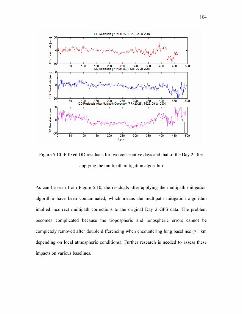
104

Figure 5.10 IF fixed DD residuals for two consecutive days and that of the Day 2 after

applying the multipath mitigation algorithm

As can be seen from Figure 5.10, the residuals after applying the multipath mitigation

algorithm have been contaminated, which means the multipath mitigation algorithm

implied incorrect multipath corrections to the original Day 2 GPS data. The problem

becomes complicated because the tropospheric and ionospheric errors cannot be

completely removed after double differencing when encountering long baselines (>1 km

depending on local atmospheric conditions). Further research is needed to assess these

impacts on various baselines.

105

As has been discussed in Section 4.2, averaging (or long term filtering) over a long

period of time is another efficient method for carrier phase multipath mitigation. It can be

expected that the impact of multipath on the positioning accuracy became insignificant

after batch processing over 12-hours worth of data. This is confirmed by calculating the

mean value of the generated IF fixed DD residuals for each satellite pair. All the mean

values are less than 1 mm.

5.9 Repeatability Analysis

In the summer 2004 campaign, all the measured benchmarks were occupied twice.

Moreover, there was always one GPS receiver held fixed to connect between sessions.

Therefore, four of the six measured benchmarks were occupied four times. A

repeatability analysis can be used as an external check for GPS positioning accuracy in

the target area.

Table 5.7 summarizes the four days’ station coordinates from Bernese for station T631

using mode 3 in Table 5.6. The coordinates for Days 2-4 are given as differences with

respect to the estimated coordinates for Day 1. Since it is unlikely that any deformation

happened during this four-day period, the repeatability of the estimated station

coordinates represents the GPS position accuracy in the target area.

As can be seen from the table, the variation of the four days station coordinates

estimation is below 1 cm. In particular, the horizontal variation of the estimated station

coordinates is less than 2 mm. Throughout this thesis, since no horizontal ground truth

106

was gathered for the measured benchmarks, the analysis is unable to determine the

planimetric positioning accuracy of GPS in the target area. The repeatability analysis

provides an accuracy measure for GPS positioning. On the other hand, the variation of

the estimated station coordinates in the height component is slightly larger, at around 7

mm. This is in agreement with the results when using precise levelling as an external

accuracy measure for the GPS estimated station height in Section 5.9 (see Table 5.8).

Table 5.7 Four days’ station coordinates from Bernese for station T631 using mode 3 in

Table 5.6. The coordinates for Days 2-4 were all given in the difference with respect to

the coordinates for Day 1 in metres.

Day 1 Day 2 Day 3 Day 4

X (m) -1627743.9304 +0.0005 -0.0002 +0.0020

Y (m) -1699512.0374 +0.0005 +0.0002 +0.0010

Z (m) 5908272.8158 +0.0008 -0.0039 -0.0069

Lat 68 24 52.272771 +0.0009 -0.0014 -0.0005

Lon -133 45 51.607776 +0.0001 -0.0003 +0.0007

Height (m) 16.2421 +0.0005 -0.0036 -0.0072

From the above repeatability analysis, it can be concluded that the positioning accuracy

of GPS in the target area is approximately 2 mm in the horizontal and 7 mm in the

vertical.

107

5.10 Developing the Best Strategy

From the foregoing results and analysis, the proposed strategy for field survey and data

processing would be:

1. Processing using mode 3 (Table 5.6),

2. Using the same type of rover antenna throughout the campaign to avoid

uncorrected PCV effects,

3. Using GPS receivers adopting semi-codeless tracking technology to avoid

significant loss of track problem in the target area,

4. Using a 15° cut-off angle, which gave the best balance between satellite geometry

and errors due to different path lengths for both 15 km and 130 km baselines on

days of both low- and high- ionospheric activity,

5. EDW correction switched off, since it was found to have insignificant or even

deleterious effects on the levelling results.

After processing all collected data using the most appropriate strategy developed in

Section 4.3, the results were compared with the levelling measurements collected in the

summer 2004. For comparison purposes, the processing results from both the 2003 and

2004 campaigns were shown in Table 5.8.

By examining the GPS height estimation using precise levelling results, the attainable

accuracy of GPS positioning in the height component by adopting the developed best

strategy for data collection and processing was found to be 2 mm with a standard

deviation of 8 mm. As has been found in the stability analysis of different survey

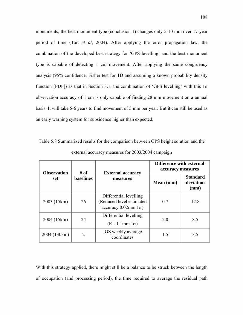
108

monuments, the best monument type (conclusion 1) changes only 5-10 mm over 17-year

period of time (Tait et al, 2004). After applying the error propagation law, the

combination of the developed best strategy for ‘GPS levelling’ and the best monument

type is capable of detecting 1 cm movement. After applying the same congruency

analysis (95% confidence, Fisher test for 1D and assuming a known probability density

function [PDF]) as that in Section 3.1, the combination of ‘GPS levelling’ with this 1σ

observation accuracy of 1 cm is only capable of finding 28 mm movement on a annual

basis. It will take 5-6 years to find movement of 5 mm per year. But it can still be used as

an early warning system for subsidence higher than expected.

Table 5.8 Summarized results for the comparison between GPS height solution and the

external accuracy measures for 2003/2004 campaign

Difference with external accuracy measures

Observation set

# of baselines

External accuracy measures

Mean (mm) Standard deviation

(mm)

2003 (15km) 26 Differential levelling

(Reduced level estimated accuracy 0.02mm 1σ)

0.7 12.8

2004 (15km) 24 Differential levelling

(RL 1.1mm 1σ) 2.0 8.5

2004 (130km) 2 IGS weekly average coordinates 1.5 3.5

With this strategy applied, there might still be a balance to be struck between the length

of occupation (and processing period), the time required to average the residual path

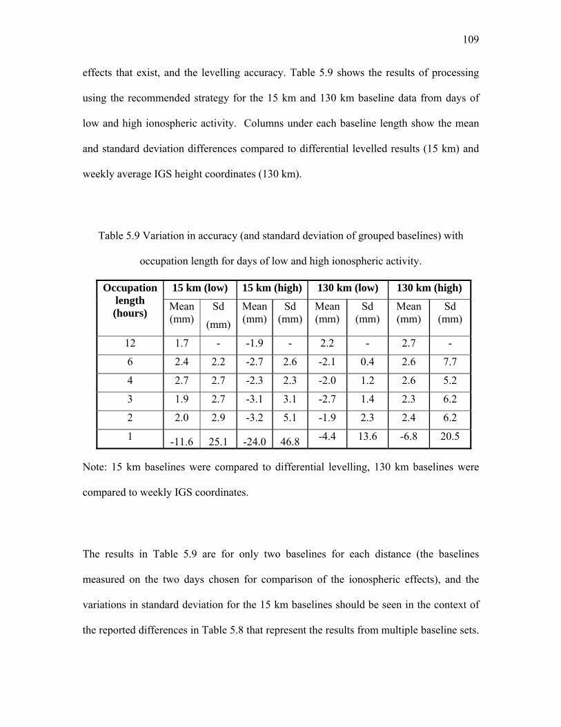
109

effects that exist, and the levelling accuracy. Table 5.9 shows the results of processing

using the recommended strategy for the 15 km and 130 km baseline data from days of

low and high ionospheric activity. Columns under each baseline length show the mean

and standard deviation differences compared to differential levelled results (15 km) and

weekly average IGS height coordinates (130 km).

Table 5.9 Variation in accuracy (and standard deviation of grouped baselines) with

occupation length for days of low and high ionospheric activity.

15 km (low) 15 km (high) 130 km (low) 130 km (high) Occupation length (hours) Mean

(mm) Sd

(mm)

Mean (mm)

Sd (mm)

Mean (mm)

Sd (mm)

Mean (mm)

Sd (mm)

12 1.7 - -1.9 - 2.2 - 2.7 -

6 2.4 2.2 -2.7 2.6 -2.1 0.4 2.6 7.7

4 2.7 2.7 -2.3 2.3 -2.0 1.2 2.6 5.2

3 1.9 2.7 -3.1 3.1 -2.7 1.4 2.3 6.2

2 2.0 2.9 -3.2 5.1 -1.9 2.3 2.4 6.2

1 -11.6 25.1 -24.0 46.8 -4.4 13.6 -6.8 20.5

Note: 15 km baselines were compared to differential levelling, 130 km baselines were

compared to weekly IGS coordinates.

The results in Table 5.9 are for only two baselines for each distance (the baselines

measured on the two days chosen for comparison of the ionospheric effects), and the

variations in standard deviation for the 15 km baselines should be seen in the context of

the reported differences in Table 5.8 that represent the results from multiple baseline sets.

110

So, for the standard deviation of 8.5 mm given in Table 5.8, the standard deviation can be

expected to increase marginally with decreasing occupation length up until the 1-hour

session, when large increases in standard deviation are evident. The results for the 130

km baselines incorporate the estimation of only one parameter, so the standard deviations

would be expected to be better than in the 15 km differential case where two rover

stations are varying. With the chosen strategy, the effect of high ionospheric activity is

minimal until 2 hours for the 15 km baselines, but the effect on the 130 km baseline is

evident throughout. So, for baselines of this length it is recommended that the survey be

planned on a day of relative inactivity according to on-line data at the Geological Survey

Canada (http://www.geolab.nrcan.gc.ca/myservlet/geomag/magnetogram/dataplot_geoma

g_e.jsp).

111

CHAPTER 6

CONCLUSIONS AND RECOMMENDATIONS

The contribution of this research was to find the attainable positioning accuracy of GPS,

especially for the height component, in the far North of Canada. By studying the

feasibility of replacing precise levelling with GPS for permafrost deformation monitoring,

the attainable ‘GPS levelling’ accuracy under poor satellite geometry and intense

ionospheric activity was investigated. At the same time this research quantified, for the

first time, the stability of monuments in permafrost, which knowledge plays a important

role not only in the future analysis of movement due to oil and gas extraction and hence

its affect on the environment, but also in the analysis of climate change effects in

permafrost areas where stable stations over long periods is required.

The feasibility study of replacing precise levelling with GPS for permafrost deformation

monitoring has been carried out by investigating the impact of different error sources on

the accuracy of GPS positioning in the target area. An analysis of the results led to the

development of an optimised strategy for data capture and processing for the target area.

Based on the research, the following conclusions address the findings in both the long

term stability study of different survey monument in permafrost and the feasibility of

replacing precise levelling with GPS for permafrost deformation monitoring.

6.1 Conclusions

The following conclusions have been made to the foregoing research:

112

1. It has been found that the use of solid ground rods founded at 5.5 m or deeper will

display similar movement pattern which is independent of the geological

conditions in which they are founded. These types of benchmarks are therefore

recommended for long-term monitoring.

2. The estimated station height error introduced by the uncorrected antenna PCV in

the IF solution for a 5 m baseline measured using different antenna type at base

and rover station was at 1 cm level. The influence of this type of error source can

be enlarged if different types of antenna were used. To avoid this problem, it is

recommended to use only one type of antenna for data collection.

3. Significant loss-of-track problems were found in the Trimble 4000SSI receivers,

which adopts codeless technology to track the L2 signal. It is much better in the

case of Ashtech Z-12 receivers which adopt semi-codeless technology. It is

recommended to use GPS receivers adopting semi-codeless technology for data

collection in the target area. Of course, this will be mitigated when the L2C is

available.

4. An elevation dependent weighting scheme is not recommended for data

processing, since it was found to have insignificant or even deleterious effects on

the levelling results.

5. The best cut-off angle used for data processing was found to be 15 degrees,

balancing longer-path observations (and higher associated atmospheric errors)

against the geometry of the satellite constellation.

6. By processing two 130 km baselines in both a low- and high- ionosphere

conditions, no accuracy degradation was found on the station height estimation

113

for a 12 hour occupation. However, when shortening the occupation length to 6

hours or less, a degradation in positioning accuracy is evident.

7. The best tropospheric delay estimation strategy was found by making use of

measured station height differences from precise levelling to examine the station

height estimation from GPS using different tropospheric delay estimation

strategies. Mode 3 in Table 5.6 was recommended for data processing. In Mode 3,

Saastamoinen tropospheric model and cosZ mapping function are used to model

the tropospheric error. The residual tropospheric error is estimated every 2 hours

along with other unknown parameters at both base and rover stations.

8. A multipath mitigation algorithm which uses day-to-day correlation has been

implemented and is based on Radovanovic’s algorithm. This algorithm has shown

its success on short baseline (< 1 km) applications. However, it is not successful

on long baselines (> 1 km) under the conditions tested in this research. This

algorithm needs to be further investigated for long baseline applications. It is

found from the analysis that averaging (or long term filtering) over long period of

time is another efficient method for carrier phase multipath mitigation.

9. Repeatability analysis was used as an external check for GPS positioning

accuracy in the target area. It was found from the repeatability analysis that the

positioning accuracy of GPS in the target area is approximately 2 mm in the

horizontal and 7 mm in the vertical.

10. By examining the GPS height estimation using precise levelling results, the

attainable accuracy of GPS positioning in the height component by adopting the

developed best strategy for data collection and processing was found to be 2 mm

114

with a standard deviation of 8 mm. As has been found in the stability analysis of

different survey monuments, the best monument type (conclusion 1) changes only

5-10 mm over 17-year period of time (Tait et al, 2004). After applying the error

propagation law, the combination of the developed best strategy for ‘GPS

levelling’ and the best monument type is capable of detecting 1 cm movement.

After applying the same congruency analysis (95% confidence, Fisher test for 1D

and assuming a known probability density function [PDF]) as that in Section 3.1,

the combination of ‘GPS levelling’ with this 1σ observation accuracy of 1 cm is

only capable of finding 28 mm movement on a annual basis. It will take 5-6 years

to find movement of 5 mm per year. But it can still be used as an early warning

system for subsidence higher than expected.

6.2 Recommendations

Based on the results of this research, the following recommendations regarding

improvement of the positioning accuracy of GPS in the target area are drawn:

1. Since the significant impact of uncorrected antenna PCV has been identified, the

mitigation of this error source should be further investigated. The latest

technology is to calibrate absolute antenna PCV based on the use of an orientated

antenna and the use of special observation differences. However, this type of

product is not yet available for distribution. The performance of this type of

product needs to be evaluated.

2. Since the multipath mitigation via day-to-day correlation algorithm is not

successful in long baseline applications, this algorithm need to be further

115

investigated. Averaging (or long term filtering) can be used as an alternative for

carrier phase multipath mitigation, in which case long term occupation was

needed. In addition, if available, it is recommended to use choke ring antenna for

data collection.

3. The satellite geometry problem of GPS for the target area has been identified in

section 3.2.4. Recent work (O’Keefe, 2001) has shown that the combination of

GPS and Galileo can greatly improved the global satellite availability and satellite

geometry, especially for the target area. Therefore, it is recommended to

investigate the use GPS/Galileo combination in the future.

4. The current L2 GPS measurements by survey-grade receivers are noisier and less

continuous than those expected to be made on the new L2C signal. With the new

L2C signal to be launched on Sept 21, 2005, the need to measure L2 using

codeless technique will have passed, and the reliability of dual frequency

operation will be enhanced (Rizos et al, 2005).

116

REFERENCES

Alves, P., G. Lachapelle, M.E. Cannon, J. Park, P. Park (2002). Use of Self-constrained

Ionospheric Modelling to Enhance Long Baseline Multiple Reference Station RTK

Positioning, Proceedings of ION GPS-02, September 24-27, 2002, Portland, Oregon, pp.

1388-1399.

Berry, R.M. (1976). History of Geodetic Levelling in the United States. Surveying and

Mapping, Vol. XXXVI, No.2, pp. 137-153.

Beutler, G. (1992). The Impact of the International GPS Service for Geodynamics on the

Surveying and Mapping Community. In: International Union of Surveying and Mapping

(IUSM) Presented apers of the Working Group Sessions, pp. 84-94.

Biacs, Z.F. (1989). Estimation and Hypothesis Testing for Deformation Analysis in

Special Purpose Networks. Master Thesis, Department of Geomatics Engineering,

University of Calgary, Alberta, Canada, UCGE Reports Number 20032.

Braasch, M.S. (1996). Multipath Effects, in Global Positioning System: Theory and

Applications Volume 1, Eds. Parkinson, B., Spiker, J., Axelrad, P, Enge, P., American

Institute of Aeronautics and Astronautics, pp. 547-568.

117

Brunner F.K., Hartinger H., and Troyer L. (1999). GPS Signal Diffraction Modelling:

The Stochastic SIGMA-∆ Model. Journal of Geodesy 73: pp. 259-267

Caspary, W. (1987). Concepts of Network and Deformation Analysis. University of New

South Wales. Monograph No. 11, Kensington, N.S.W.

Cannon, M.E. and Lachapelle, G. (2003). GPS Positioning, ENGO 561 Lecture Notes,

Department of Geomatics Engineering, The University of Calgary, Calgary, Alberta.

Chen, D. and Lachapelle, G. (1994), A Comparison of the FASF and Least-Squares

Search Algorithms for On-the-Fly Ambiguity Resolution. Journal of the Institute of

Navigation, Vol. 42, No.2, pp. 371-390.

Collins, J. (1989). The Satellite Solution to Surveying. Professional Surveyor. No. 2. Vol.

6. pp. 12-17.

Counselman, C., Shapiro, I., Greenspan, R., Cox, D. (1979). Astronomical application of

differential interferometry. Science, No. 178. pp. 607-608.

Francisco, S.G. (1996). GPS Operational Control Segment. In: Global Positioning

System : Theory and Applications : Volume 1. Parkinson, B. and Spilker, J., eds.

American Institute of Aeronautics and Astronautics. pp. 435-465.

118

Fotopoulos, G. (2003). An Analysis on the Optimal Combination of Geoid, Orthometric

and Ellipsoidal Heigth Data. PhD Thesis, Department of Geomatics Engineering,

University of Calgary, Alberta, Canada, UCGE Reports Number 20185.

Fortes, L. (2002). Optimising the Use of GPS Multi-Reference Stations for Kinematic

Positioning. PhD Thesis, Department of Geomatics Engineering, University of Calgary,

Alberta, Canada, UCGE Reports Number 20158.

Gareau, R.M. (1986): History of Precise Levelling in Canada and The North American

Vertical Datum Readjustment. MSc Thesis, Department of Geomatics Engineering,

University of Calgary, Alberta, Canada, UCSE Reports Number 20018.

Gili, J.A., Corominas, J. and Rius, J. (2000). Using Global Positioning System

Techniques in Landslide Monitoring, Engineering Geology, Vol 55, pp. 167-192.

Guo, J. and Ge, S. (1997). Research of Displacement and Frequency of Tall Building

under Wind Load Using GPS. In: Proceedings of the 10th International Technical

Meeting of the Satellite Division of the Institute of Navigation. pp. 1385-1388.

Hartinger, H., Brunner, F.K. (1998). Experimental detection of deformations using GPS.

In : Kahmen H, Brückl E, Wunderlich T (eds) Geodesy for Geotechnical and Structural

Engineering. Proc. IAG Special Commission 4 Symposium Eisenstadt, pp. 145-152.

119

Hartinger H, Brunner FK (1999) Variances of GPS Phase Observations: The SIGMA-ε

Model. GPS Solutions 2/4: pp. 35-43.

Hartinger, H., Brunner, F.K. (2000). Development of a monitoring system of landslide

motions using GPS. In: Proc 9th FIG Symposium on Deformation Measurements,

Olsztyn, Sept. 1999, pp. 29-38.

Hedling, G., Jonsson, B., Lilje, C., and Lilje, M. (2001). SWEPOS – The Swedish

Network of Permanent GPS reference Station (Status February 2001). International

Conference on New technology for a New Century. FIG Working Week 2001. 6-11 May

2001. Seoul, Korea.

Heiskanen, W.A. and Moritz, H. (1967). Physical Geodesy. W.H. Freeman and Company

San Francisco.

Hofmann-Wellenhof, B., Lichtenegger, H. and Collins, J. (2001). GPS: Theory and

Practice. Second Edition. Springer-Verlag.

Hopfield, H.S. (1970). Tropospheric Effect on Electromagnetically Measured Range:

Prediction from Surface Weather Data, Applied Physics Laboratory, Johns Hopkins

University, Baltimore, MD.

Hopfield, H.S. (1972). Tropospheric Range Error Parameters-Further Studies, Applied

120

Physics Laboratory, Johns Hopkins University, Baltimore, MD.

Hoyle, V.A. (2004). Personal communication.

Hudnut, K.W. (1996). Continuous GPS monitoring of dam deformation. EOS, Trans.

AGU, 77, No. 46, pp. F139.

Hudnut, K.W. and Behr, J.A. (1998). Continuous GPS monitoring of structural

deformation at Pacoima Dam, California, Seismological Research Letters, 69, No. 4, pp.

299-308.

Hugentobler, U., S. Schaer, P. Fridez (2001). Bernese GPS Software Version 4.2.

Astronomical Institute, University of Berne.

ICD-GPS-200C (2003). Navstar GPS Space Segment / Navigation User Interfaces.,

Revision C. GPS NAVSTAR JPO. January, 2003.

Janssen, V., Roberts, C., Rizos, C., and Abidin, H. (2001). Experiences with a mixed-

mode GPS-based volcano monitoring system at Mt. Papandayan, Indonesia. Geomatics

Research Australasia, 74, pp. 43-58.

Kaplan, D (1996). Understanding GPS Principles and Applications, Artech House

Publishers, Boston, pp. 351.

121

Kenselaar, F. and Quadvlieg, R. (2001). Trend Signal Modelling of Land Subsidence.

Proceedings of the 10th International Symposium on Deformation Measurements, Orange,

California, USA, 19-22 March, 2001.

Klobuchar, J.A. (1986). Design and Characteristics of the GPS Ionospheric time-delay

algorithm for single-frequency users. In : Proceedings of PLANS’86-Position Location

and Navigations symposium, Las Vegas, Nevada, November, pp. 280-286.

Klobuchar, J.A., Doherty, P.H., and El-Arini, M.B. (1995). Potential Ionospheric

Limitations to GPS Wide Area Augmentations System. In: Navigation, Journal of the

Institute of Navigation, Vol 42. 1995.

Klobuchar, J.A. (1996). Ionospheric Effects on GPS. In: Global Positioning System,

Theory and Application, Vol 1, Eds, Parkinson, B. and Spilker, J., American Institute of

Aeronautics and Astronautics, Inc., pp. 485-514.

Knight, M., Cervera, M., Finn A. (1999). A comparison of predicted and measured GPS

performance in an ionospheric scintillation environment. Proceeding ION GPS-99,

September 14-17 Nashville, TN, pp. 1437-1450.

Lachapelle, G. and Cannon, M.E. (2004). GPS Theory and Applications. ENGO 625

Lecture Notes. Department of Geomatics Engineering, The University of Calgary.

Langley, R. (1997). GPS Receiver System Noise. GPS World. June 1997. pp. 40-45.

122

Lanyi, G. (1984). Tropospheric Delay Effects in Radio Interferometry,

Telecommunications and Data Acquisition Progress Rep., Jet Propulsion Lab, Pasadena,

CA.

Mackay, J., Ostrick, J., Lewis, C., Machay, D. (1979). Frost heave at ground

temperatures below 0 oC, Inuvik, Northwest Territories. Paper- Geological Survey of

Canada 79-1A, pp. 403-406.

Mader, G. (1999). GPS Antenna Calibration at the National Geodetic Survey. GPS

Solutions, Vol. 3, No. 1, Summer 1999, Wiley.

Meng, X., Roberts, G.W., Dodson, A.H., Cosser, E., Barnes, J., and Rizos, C. (2004).

Impact of GPS satellite and pseudolite geometry on structural deformation monitoring:

analytical and empirical studies. Journal of geodesy, 77, pp. 809-822.

Menge, F., G. Seeber, C. Völksen, G. Wübbena, M. Schmitz (1998). Results of Absolute

Field Calibration of GPS Antenna PCV, In: Proceedings of the 11th International

Technical Meeting of the Satellite Division of the Institute of Navigation ION GPS-98,

September 15-18, Nashville, Tennessee, 1998.

Moorman, B. and P. Vachon. (1998). Detecting ground ice melt with interferometric

synthetic aperture radar. 20th Canadian Symposium on Remote Sensing, Calgary, Alberta,

May 10-13, 1998.

123

Moorman, B., Vachon, P., Sjogren, D. (2003). Monitoring permafrost degradation and

ground surface movement with interferometric synthetic aperture radar. Proceedings, 8th

International Conference on Permafrost, Zurich, July 21-25, 2003.

Muller, S.W. (1943). Permafrost or permanently frozen ground andrelated engineering

problems. U.S. Army, Office Chief of Engineers, Military Intelligence Div. Strategic Eng.

Study 62, pp. 231. (Also 1947, Ann Arbor, Mich., Edwards Bros.)

Nichols, J.A., Hansen, A., Walter, T., Enge, P.K. (1999). High latitude measurements of

ionospheric scintillation using the NSTB. Proceeding ION Nat Tech Meeting, January

25-27 San Diego, CA, pp. 789-798.

O'Keefe, K. (2001). Availability and Reliability Advantages of Galileo/GPS Integration.

Proceedings of the Satellite Division of the Institute of Navigation 14th International

Technical Meeting (September 11-14, 2001, Salt Lake City, Utah), pp. 2096-2104.

Parkinson, B.W. (1996). GPS Error Analysis, in Global Positioning System: Theory and

Applications Volume 1, Eds. Parkinson, B., Spiker, J., Axelrad, P, Enge, P., American

Institute of Aeronautics and Astronautics, pp. 469-483.

Radovanovic, R.S. (2000). High Precision Deformation Monitoring by Multipath

Mitigation via Day-To-Day Correlation Analysis. Proceedings of ION-GPS 2000, Salt

Lake City, September 10-15.

124

Radovanovic, R.S. (2002). Adjustment of satellite-based ranging observations for precise

positioning and deformation monitoring. PhD Thesis, Department of Geomatics

Engineering, University of Calgary, Alberta, Canada, UCGE Reports Number 20166.

Raquet, J. (1998), Development of a Method for Kinematic GPS Carrier-Phase

Ambiguity Resolution Using Multiple Reference Receivers. Ph.D. Thesis, University of

Calgary, Department of Geomatics Engineering Report Number 20116, Calgary 1998.

Ray, J.K. (2000). Mitigation of GPS Code and Carrier Phase Multipath Effects Using a

Multi-Antenna System. PhD Thesis, Department of Geomatics Engineering, University

of Calgary, Alberta, Canada, UCGE Reports Number 20136.

Remondi, B. (1984). Using the Global Positioning System Phase Observable for Relative

Geodesy : Modelling, Processing and Results. Ph.D. Dissertation. Austin: Centre for

Space Research, University of Texas at Austin.

Rempel, G. (1970). Arctic terrain and oil field development. Proceedings of the American

Geological Institute Conference on Productivity, pp. 243-251

Rizos, C. (1999). Satellite Ephemeris Bias. Principles and Practice of GPS Surveying.

The University of New South Wales, Sydney, Australia. http://www.gmat.unsw.edu.au/

snap/gps/gps_survey/chap6/6212.htm (last updated: 18 January 2000)

125

Rizos, C., Higgins, M., and Hewitson, S. (2005). New GNSS Developments and their

Impact on Survey Service Providers and Surveyors. Proceedings of SSC2005 Spatial

Intelligence, Innovation and Praxis: The national biennial Conference of the Spatial

Sciences Institute, September 2005. Melbourne: Spatial Sciences Institute. ISBN 0-

9581366-2-9.

Roberts, C. and Rizos, C. (2001). Mitigating differential tropospheric effects for GPS-

based volcano monitoring. In: proceedings of the 5th Symposium on Satellite Navigation

Technology and Applications, Canberra, Australia, 24-27 July, paper 38, CD ROM

proceedings.

Rostoker, G. and Skone, S. (1993). Magnetic flux mapping considerations in the auroral

oval and the Earth's magnetotail. J Geophys Res 98(A2): pp. 1377-1384.

Roulston, A., Nicholas, T., Zhang, k. (2000). An Evaluation of Various GPS Satellite

Ephemerides, In Proceedings of ION GPS 00, Salt Lake City, pp. 45-54.

Saastamoinen, J. (1972). Atmospheric Correction for the Troposphere and stratosphere in

Radio Ranging of Satellites, Geophysical Monograph 15, American Goephysical Union,

Washington DC.

Seeber, G. (1993) Satellite Geodesy, Foundations, Methods, and Applications. Walter de

Gruyer.

126

Skone, S. (1998). Wide Area Ionosphere Grid Modelling in the Auroral Region, Ph.D.

thesis, Department of Geomatics Engineering, University of Calgary, Calgary, AB

Skone, S. and M. de Jong (2000). The Impact of Geomagnetic Substorms on GPS

Receiver Performance. In: Earth Planets Space, 52, pp. 1067–1071.

Skone, S. (2001). The Impact of Magnetic Storms on GPS Receiver Performance. In

Journal of Geodesy. 75: pp. 457-468.

Skone, S., K. Knudsen and M. de Jong. (2001). Limitations in GPS receiver tracking

performance under ionospheric scintillation conditions. In Physics and Chemistry of the

Earth, vol. Part A, 26/6-8, pp. 613-621.

Skone, S. (2003). Atmospheric Effects on Satellite Navigation Systems. ENGO 633

Lecture Notes, Department of Geomatics Engineering, The University of Calgary.

Smith, S.L., Burgess, M.M., Heginbottom, J.A. (2001). Permafrost in Canada, a

challenge to northern development. In: Brooks, G.R. (ED.), A synthesis of Geological

Hazards in Canada, Geological Survey of Canada, Bulletin, vol. 548, pp. 241-264.

Spilker, J.J., Jr. (1994). Tropospheric Effects on GPS, in Global Positioning System:

Theory and Applications Volume 1, Eds. Parkinson, B., Spiker, J., Axelrad, P, Enge, P.,

American Institute of Aeronautics and Astronautics, pp. 517-546.

127

Tait, M., Moorman, B. (2003). A feasibility study into monitoring deformation in the

Niglintgak region of the Machenzie delta. Proceedings of the 11th FIG Symposium on

Deformation Measurement, 25-29 May 2003, Santorini, Greece.

Tait, M. (2004). Geomatics Networks. ENGO 519 Lecture Notes. Department of

Geomatics Engineering, The University of Calgary.

Tait, M., Sheng, L., Cannon, M.E. (2004) The feasibility of replacing precise levelling

with GPS for permafrost deformation monitoring. Proceedings of the FIG 3rd

International Conference on Engineering Surveying, Bratislava, Slovakia, November 11-

13.

Tait, M., Moorman, B., and Sheng, L. (2005). The long-term stability of survey

monuments in permafrost. Engineering Geology, Vol. 79, pp. 61-79.

Teunissen, P.J.G. and Tiberius, C.C.J.M. (1994). Integer Least-Squares Estimation of The

GPS Phase Ambiguities. Proceedings of the International Symposium on Kinematic

Systems in Geodesy, Geomatics and Navigation, Department of Geomatics Engineering,

The University of Calgary, pp. 221-231.

Wang, Z. and S. Li. (1999). Detection of Winter Frost Heaving of the Active Layer of

Arctic Permafrost Using SAR Differential Interferometry. Proceedings of IEEE 1999

128

International Geoscience and Remote Sensing Symposium 1999 (IGARSS ’99). 28 June-

2 July, 1999, Hamburg, Germany. pp. 1946-1948.

Wieser, A., Brunner, F.K. (2002). Analysis of Bridge Deformations using Continuous

GPS Measurements. INGEO2002, 2nd Conference of Engineering Surveying, Kopáčik A

and Kyrinovič P (eds), Bratislava, November 2002, pp. 45-52.

Wooden, W.H. (1985). Navstar Global Positioning System: 1985, Proceedings of the

First International Symposium on Precise Positioning with the Global Positioning System,

Rockville, Maryland, 1985.

Wübbena, G., Schmitz, M., Menge, F., Böder, H., Seeber, G. (2000). Automated

Absolute Field Calibration of GPS Antennas in Real-time. Presented at ION GPS-00, 19-

22 September, Salt Lake City, Utah, USA.

Wübbena G., Gagge, A., Boettcher, G., Schmitz, M., Andree, P. (2001). Permanent

Object Monitoring with GPS with 1 Millimetre Accuracy. Presented at the International

Technical Meeting, ION GPS-01, September 11-14, 2001, Salt Lake City, Utah.

Yunck, T.P. (1993). Coping with the atmosphere and ionosphere in precise satellite and

ground positioning. In: Geophys. Monograph 73, Environmental effects on spacecraft

positioning and trajectories, AGU, IUGG Vol. 13, pp. 1-16.

129

APPENDIX 1: A SUMMARY OF THE TYPE OF MONUMENT

# Type Depth (m)

Method Drilling report (June 1987)

Permafrost surface Oct 1987 (m)

621 CCGR 15 D Permafrost from 0.6m Solid ice 3m – 3.6m Very hard clay 6m – 7.5m Fine / dry clay 12m +

0.2

622 AGR 2 J 0.25 623 CCGR 5.5 D Permafrost from 0.9m

Mud-like clay until 2.5m Heavy ice content 2.5m +

0.25

624 CCGR 9 D Permafrost from 0.6m High content of small gravel throughout

0.18

625 ReeBar (φ19mm)

0.9 J 0.25

626 SFAP 0.6 J 0.2 627 DBM 14.5 D Permafrost from 1.5m

Frozen clay to 4.5m Ice/clay mix 4.5m – 9m Mostly ice to 14m Frozen clay to 14.5m

>0.45

628 CCGR 8.7 J 0.22 629 CCGR 4.5 J 0.2 630 CCGR 2.7 J 0.2 631 DBM 17.5 D Permafrost from 0.9m

Very dry clay throughout 0.45

632 CCGR 1.8 J 0.2 633 CCGR 1.5 J 0.2 634 AGR 5.5 J 0.4 635 AGR 1.5 J 0.15 636 HELIX 2.5 D Permafrost from 1.2m

Very high moisture content throughout

0.15

637 DBM 8 D Permafrost from 0.6m Very sticky clay throughout

0.15

638 IPBC 1.5 D None 0.13 639 DBM 6.9 D Permafrost from 0.6m

High ice content 3m – 4.3m Frozen gravel (?) 4.3m – 4.9m

>0.45

640 IPBC 0.75 D None 0.25

641 IPBC 0.75 D None 0.25