university of sydney school of physics...

University of SydneySchool of Physics

SUPPLEMENTARY NOTESfor

Senior Experimental Physics Handbook

July 25, 2007

These notes are for students enrolled in any of the following units of study. The credit point numberindicates the number of credit points allocated to the Physics lab component of the unit:

Semester 1

PHYS 3040, 3940 Electromagnetism & Lab (4 credit points)

PHYS 3051, 3951 Thermodynamics/Biol. Physics & Lab (2 credit points)

PHYS 3054,3954 Nanoscience/Plasma Physics & Lab (2 credit points)

Semester 2

PHYS 3060, 3960 Quantum Mechanics & Lab (4 credit points)

PHYS 3062, 3962 Quantum Mechanics/Cond. Matter Physics & Lab (2 credit points)

PHYS 3068, 3968 Optics/Cond. Matter Physics & Lab (2 credit points)

PHYS 3069, 3969 Optics/High Energy Physics & Lab (2 credit points)

PHYS 3071, 3971 High Energy/Astrophysics & Lab (2 credit points)

PHYS 3074, 3974 High Energy/Cond. Matter & Lab (2 credit points)

1

2 SENIOR PHYSICS LABORATORY

Contents

1 THE WIB SMITH PRIZE FOR EXPERIMENTAL PHYSICS 4

2 LABORATORY RULES AND ADVICE 42.1 Laboratory equipment . . . . . . . . . . . . . . . . . . . . . . . . . . . . . . . . . 52.2 Laboratory library . . . . . . . . . . . . . . . . . . . . . . . . . . . . . . . . . . . 5

3 LABORATORY SAFETY 53.1 Fire: whole laboratory complex . . . . . . . . . . . . . . . . . . . . . . . . . . . . 53.2 Toxic Materials e.g. X-Ray Diffraction and Holography experiments . . . . . . . . 53.3 Microwave Radiation: Wave Propagation and Microwave experiments . . . . . . . 53.4 Laser Radiation: Optical Images and Holography experiments . . . . . . . . . . . 63.5 Ionising Radiation X-Ray Diffraction, Alpha Particles, Mossbauer, Cosmic Rays,

Nuclear Lifetimes, Gamma Rays, Beta Particles and X-Rays experiments . . . . . 6

4 GUIDELINES FOR RECORDING EXPERIMENTAL WORK 74.1 INTRODUCTION . . . . . . . . . . . . . . . . . . . . . . . . . . . . . . . . . . 74.2 GENERAL . . . . . . . . . . . . . . . . . . . . . . . . . . . . . . . . . . . . . . 74.3 LOGBOOKS . . . . . . . . . . . . . . . . . . . . . . . . . . . . . . . . . . . . . 7

4.3.1 Description of Experimental Work . . . . . . . . . . . . . . . . . . . . . . 74.3.2 Records of Observations and Data . . . . . . . . . . . . . . . . . . . . . . 84.3.3 Tables . . . . . . . . . . . . . . . . . . . . . . . . . . . . . . . . . . . . . 84.3.4 Graphs . . . . . . . . . . . . . . . . . . . . . . . . . . . . . . . . . . . . 84.3.5 Analysis of data . . . . . . . . . . . . . . . . . . . . . . . . . . . . . . . . 94.3.6 Results . . . . . . . . . . . . . . . . . . . . . . . . . . . . . . . . . . . . 94.3.7 Conclusions . . . . . . . . . . . . . . . . . . . . . . . . . . . . . . . . . . 9

5 DATA ANALYSIS 105.1 Introduction . . . . . . . . . . . . . . . . . . . . . . . . . . . . . . . . . . . . . . 105.2 Confidence intervals . . . . . . . . . . . . . . . . . . . . . . . . . . . . . . . . . 105.3 Systematic Errors . . . . . . . . . . . . . . . . . . . . . . . . . . . . . . . . . . . 11

5.3.1 Sources of error - meter and oscilloscope errors . . . . . . . . . . . . . . . 125.3.2 Combining systematic errors . . . . . . . . . . . . . . . . . . . . . . . . . 13

5.4 Random errors . . . . . . . . . . . . . . . . . . . . . . . . . . . . . . . . . . . . 155.5 Probability distributions . . . . . . . . . . . . . . . . . . . . . . . . . . . . . . . . 16

5.5.1 The normal distribution . . . . . . . . . . . . . . . . . . . . . . . . . . . . 165.5.2 The Poisson distribution . . . . . . . . . . . . . . . . . . . . . . . . . . . 17

5.6 The statistics of data samples . . . . . . . . . . . . . . . . . . . . . . . . . . . . . 175.6.1 The sample mean . . . . . . . . . . . . . . . . . . . . . . . . . . . . . . . 175.6.2 The sample standard deviation . . . . . . . . . . . . . . . . . . . . . . . . 185.6.3 Standard error of the mean . . . . . . . . . . . . . . . . . . . . . . . . . . 18

5.7 Confidence intervals and statistical tests . . . . . . . . . . . . . . . . . . . . . . . 195.7.1 The confidence interval for the mean . . . . . . . . . . . . . . . . . . . . . 195.7.2 The confidence interval for the standard deviation . . . . . . . . . . . . . . 215.7.3 Statistical test . . . . . . . . . . . . . . . . . . . . . . . . . . . . . . . . . 215.7.4 Tests for the mean and standard deviation . . . . . . . . . . . . . . . . . . 225.7.5 Rejection of data . . . . . . . . . . . . . . . . . . . . . . . . . . . . . . . 225.7.6 The χ2 goodness-of-fit test . . . . . . . . . . . . . . . . . . . . . . . . . . 23

5.8 Combining statistical errors . . . . . . . . . . . . . . . . . . . . . . . . . . . . . . 26

SUPPLEMENTARY NOTES 3

5.9 Errors and graphs . . . . . . . . . . . . . . . . . . . . . . . . . . . . . . . . . . . 275.9.1 The method of least squares . . . . . . . . . . . . . . . . . . . . . . . . . 275.9.2 Confidence intervals for the slope and intercept . . . . . . . . . . . . . . . 285.9.3 A word of warning . . . . . . . . . . . . . . . . . . . . . . . . . . . . . . 29

5.10 Slopes and intercepts . . . . . . . . . . . . . . . . . . . . . . . . . . . . . . . . . 30

6 SOME USEFUL PHYSICAL CONSTANTS 31

7 SI PREFIXES 31


1 THE WIB SMITH PRIZE FOR EXPERIMENTAL PHYSICS

WIB Smith, known to all as WIBS, was a senior lecturer in Physics from 1963 to 1981 and wasan exceptionally good tutor in the Senior Physics laboratory. He believed that (nearly) all physicscould be described in a simple manner if some effort was put into it. He had a great talent forcommunicating with students in this way.

After WIBS’ tragic death in 1983, his friends and colleagues contributed a substantial sum of moneyto establish a prize in his memory. It is awarded to the student who best combines the characteris-tics of experimental skill, proficiency and exceptional motivation in the Senior Physics laboratory,providing that person shows sufficient merit. The tutors become aware of a student’s motivationduring discussions about experiments, particularly of the physics involved in an experiment.

This prize is normally awarded to a student taking at least 8 credit points of experimental physicsunits in the course of the year.

2 LABORATORY RULES AND ADVICE

(a) At the beginning of the semester you will be supplied with general introductory notes. Notesfor each experiment will be supplied as required throughout the year. It is essential to readcarefully the notes on an experiment before you start work - the night before is suggested.Do not expect every step in the procedure to be described. However, if you understand thephysics in advance, your activities in the laboratory will run smoothly and efficiently.

(b) No smoking, eating or drinking except in the area allocated for tea or coffee. Leave wet clothingetc. outside the laboratory.

(c) Turn off the power from main sockets when you leave the laboratory at the end of an afternoon’swork. You can leave plugs in plugboard sockets. Turn off all battery operated equipment.

(d) It helps to set the apparatus out neatly.

(e) Equipment is not to be moved from one bench to another. Please report any deficiencies to astaff member.

(f) A reasonable standard of dress is expected; in particular, shoes must be worn. Although all theapparatus is safe, with any mains operated electrical equipment there could be an extremelysmall but finite risk of electric shock. Non-conducting shoes are a definite advantage in thisrespect. They also protect your toes in the unlikely event of a heavy piece of equipment beingtipped off a bench! Handle the high voltage equipment with care. If a malfunction occurs donot remove protective covers, call a staff member.

(g) A student who is sick may be allowed to skip an experiment if a medical certificate is providedwithin a reasonable time. Please check out individual cases with the laboratory supervisor. Insuch cases a Request for Special Consideration should be submitted.

(h) Do not remove bench notes for an experiment from their proper place i.e. on the table for thatexperiment.


2.1 Laboratory equipment

Check that all the equipment for your experiment is available before you start (The notes of mostexperiments are headed by an equipment list).

There are a number of calculators in the laboratory that are available for use, but it would be clearlyconvenient to have your own.

There are many computers in the laboratory. Some of the laboratory’s experiments have sectionswhere the data is fed directly to one of the computers. In other experiments a computer program isneeded to process manually entered data. Further information on the use of the computers is givenin a bench file near the computers.

2.2 Laboratory library

A small number of books are kept in a cupboard near the entrance to the laboratory. Apart fromthe exception below, books may be borrowed overnight or over the weekend. Longer borrowing isnot allowed - the books could be needed by other students. Enter your name, the date and book’sauthor in the “library borrowing” pad located on the front bench. For obvious reasons we do notallow reference handbooks to leave the laboratory. The main physics library has copies of thesehandbooks for the use of students who wish to work up there.

3 LABORATORY SAFETY

The Hazards are:-

3.1 Fire: whole laboratory complex

The presence of fire will normally be indicated by automatic activation of an alarm. Leave thelaboratory in an orderly but rapid manner, helping disabled colleagues if necessary. Assemble onPhysics Road near the main door of the main physics building. Obey directions of fire wardens(persons wearing green plastic hats).

3.2 Toxic Materials e.g. X-Ray Diffraction and Holography experiments

Do not taste or ingest any samples used in the experiments. (None are really poisonous but theprinciple must be followed of course.)

3.3 Microwave Radiation: Wave Propagation and Microwave experiments

The power flux (watt per sq. metre) of this radiation is below the Australian standard limit of 0.2mW per sq. cm (for the public, 24 hour exposure). Exposure to radiation should be kept As LowAs is Reasonably Achievable (the ALARA principle): do not sit or stand so your eyes are less than30 cm from the transmitting antenna or the waveguide of the Wave Propagation experiment.


3.4 Laser Radiation: Optical Images and Holography experiments

Do not place eyes so that the beam can enter and possibly focus on the retina. Do not place spec-ularly reflecting surfaces in the laser beam; the reflected radiation could enter someone’s eye. Thelasers give about 1 mW which means that diffusely reflected radiation is safe.

3.5 Ionising Radiation X-Ray Diffraction, Alpha Particles, Mossbauer, Cosmic Rays,Nuclear Lifetimes, Gamma Rays, Beta Particles and X-Rays experiments

The absorbed dose is measured in gray (J/Kg of irradiated tissue). Heavily ionising radiation (likealpha particles) causes much more radiation damage than gamma rays or beta particles. This is al-lowed for by using the dose equivalent measured in sievert. For betas and gammas the two measuresare the same. All accessible alpha sources in the laboratory are very weak and there is no significantdanger from them.

The maximum limit for the public is 5 millisievert in one year (for radiation workers it is 50 mSvin one year, but we use the more stringent limit here). This compares with the natural radiationbackground of 1 to 2 mSv/yr. Radiation protection agencies recommend that one attempts to holdthe dose equivalent to be less than 1 mSv plus the background in one year and that the ALARAprinciple be followed (see note about microwave radiation above).

The 1 mSv plus background rule can easily be met in the laboratory by not handling the sourcesunnecessarily or for unnecessarily long times and by keeping the stronger sources in the shieldingcontainers where provided. The strongest source in the laboratory is a 40 GBq Americium Beryl-lium neutron source in the red metal box located in the south east corner of the laboratory. Otherstrong sources are kept in a lead lined radioactive safe located below the red box. The 5 mSv/yrlimit has been marked on the floor with a red band. Follow the ALARA principle: do not go intothis area unless you need to. Note that a person spending 15 minutes on every day of the year,standing on the red band would receive 0.05 mSv in addition to the greater than 1 mSv background.


4 GUIDELINES FOR RECORDING EXPERIMENTAL WORK

4.1 INTRODUCTION

The written record is a vital part of experimental work and it is inevitable that the assessment ofexperimental work in Physics Laboratories is largely based on it. When reading your record thephysics staff are trying to assess the quality of the practical work as well as that of the record itself.

The following guidelines set out what is expected in the written record of experimental work inphysics.

4.2 GENERAL

• A written record should be made directly in a permanently bound LOGBOOK while an ex-periment is actually being carried out.

• If an experiment is written up after it has been completed, using the LOGBOOK, the LAB-ORATORY NOTES (and other references if appropriate), the result is generally called aREPORT.

• In Junior, Intermediate, and Senior years your LOGBOOK will generally contain the requiredcomplete record of each experiment and you will only be expected to write REPORTS fora limited number of experiments. All of the following sections apply for LOGBOOKS inJunior, Intermediate, and Senior years.

4.3 LOGBOOKS

A LOGBOOK is a working record of experimental work and should contain sufficient informationsuch that, at any time in the future, a REPORT (see Section 1.2) could be written. It should bepossible for a ’scientifically literate person’ to understand what was done by reading the logbookrecord in conjunction with the laboratory notes for the experiment.

4.3.1 Description of Experimental Work

• The date should be recorded at the beginning of each session in the laboratory.

• Each experimental topic should be given a descriptive heading and, where appropriate, theidentifying number of the apparatus should be recorded.

• A brief introduction, description of apparatus and experimental procedures should be in-cluded. This should amount to only a few sentences. A reference can be given to the notesfor more details.

• Schematic or block (rather that pictorial) diagrams should be included where appropriate.

• Circuit diagrams should be included.


4.3.2 Records of Observations and Data

• The LOGBOOK must contain the original record of all observations and data - includingmistakes! Never erase or obliterate “incorrect” readings. Simply cross them out in such away that they can be read if need be.

• Type and serial numbers of instruments used in addition to the standard apparatus should berecorded whenever there is the possibility that measurements may have to be repeated or thecalibration checked.

• Zero readings, calibration factors, resolution limits and rated accuracies of instruments shouldbe recorded whenever they are relevant.

• Particular points regarding your experimental technique such as, for example, precautionstaken to avoid backlash or the effects of temperature changes should be noted.

• Other factors such as temperature and pressure should be recorded if there is a possibility thatthey may affect the observational data or the outcome of the experiment.

• All relevant non-numerical observations should be clearly described. A sketch should be usedwhenever it would aid the description.

• Each reading should be identified by name or defined symbol together with its numericalvalue and unit.

4.3.3 Tables

• Observations and data should be tabulated whenever appropriate.

• Each table should have an identifying caption.

• Columns in tables should be labelled with the names or symbols for both the variable and theunits in which it is measured. If a symbol is used it should be defined.

4.3.4 Graphs

• In some experiments you will get a graphical printout of data from the computer used to runthe experiment. While tabulated data can be graphed by hand, it is preferable to plot datausing Excel or preferably Origin. Both applications are available on the computers at thefront of the laboratory. Graphs should be securely fastened in the LOGBOOK.

• Each graph should have a descriptive caption, which refers to any relevant distinguishingparameters, and/or conditions, which do not appear in the graph itself.

• Axes of graphs should be labelled with the names or symbols for the quantity and its unit.Numerical values should be written along each axis. Scales should be chosen which make iteasy for intermediate values to be read quantitatively.

• Data points on graphs should be clearly identified. If more than one set of points is plottedeach set should be plotted using a different symbol. Error bars should be drawn whereverappropriate to indicate the uncertainty in each data point except in the case of a large numberof data points when an indication of typical error bars is acceptable.


• Construction points for theoretical curves should be erased or distinguished from experimen-tal points.

• Each trend line should be drawn smoothly without sharp discontinuities.

4.3.5 Analysis of data

• Calculations for each section of an experiment should be done as soon as relevant measure-ments have been completed so that it can be seen whether some measurements should berepeated.

• The organisation of calculations should be sufficiently clear for mistakes (if any) to be easilyfound.

• In cases where intermediate results of calculations need to be written down they should berecorded in the LOGBOOK. Repeated calculations of the same kind should be tabulated.

• The procedures used for estimating and combining uncertainty estimates should be clearlyspecified. Non-standard procedures should be described in detail.

4.3.6 Results

• Results should be given with an estimate of their uncertainty wherever possible. The type ornature of each uncertainty estimate should be specified unambiguously.

• Results should be compared whenever possible with accepted values or with theoretical pre-dictions.

• Serious discrepancies in results should be examined and every effort made to locate the rea-son.

4.3.7 Conclusions

• A conclusion should be written for every topic or experiment.

• The conclusion should make sense when read in isolation from the rest of the record.

• The conclusion should be consistent with the results and contain a comparison with acceptedvalues or with theoretical predictions (see Section 5.2). Any discrepancies should be dis-cussed.

• If there are specific comments to be made about the experiment or apparatus it is appropriateto include then in the Conclusions.


5 DATA ANALYSIS

5.1 Introduction

When you do an experiment in the laboratory, making observations and gathering data is only halfof the job. The proper analysis of your results is equally important. In analysing your data youshould try to achieve two aims:

• To present your results in a convenient and simple way, so that others - and you in threemonths time! - can quickly understand what you did.

• To assess your confidence in the results by analysing the errors which are present and deter-mining how they affect your conclusions.

By now you should be familiar with the basic skills of tabulating and graphing data, determiningslopes, etc., so we will be chiefly concerned with the second of these two points - error analysis. Itshould be emphasised that there is no magic formula which can always be used, but it is difficult toproceed without some knowledge of statistical methods, and when they may and may not be used.The purpose of these notes is to introduce some of the formal techniques for dealing with exper-imental data while still retaining an overall emphasis on commonsense and logic as the principalingredients of “good” data analysis.

You should regard data analysis as an integral part of your experimental work, not something thatis tacked on at the end. Good experimental scientists always analyse their results as they go along.There are many reasons for this, but perhaps the most important are:

• checking your work as you progress through an experiment is an excellent way to detect andcorrect mistakes at an early stage, thereby minimising time lost in repeating work; and

• it is easy to overlook some vital piece of information (e.g. a voltage setting, the range multi-plier switch on a digital multimeter, etc.) and by working up your data immediately, while theapparatus is still set up, you can catch these oversights and record the necessary information.

5.2 Confidence intervals

We express our confidence in results by using “confidence intervals. For example, an energy differ-ence might be given as (2.57 ± 0.14) × 10−3 J.

The range 2.43 mJ to 2.71 mJ is the confidence interval for this quantity; the limits ± 0.14 mJ areoften called the confidence limits. What this means is that the experimenter is reasonably sure thatthe “true” value of the energy difference lies within the stated range.

Confidence intervals go by many names: limits of accuracy, tolerance bands, error limits, etc., areall used. In any case, the general idea is always the same. The interval represents some kind ofestimate of the confidence that the true value lies within the indicated range.

There are two pitfalls to be avoided. The optimistic physicist implicitly trusts the equipment andalways quotes small confidence limits, and is also invariably wrong. The pessimist takes the oppo-site view, giving 3 ± 3 mJ as the answer to our example. These limits are so large as to be useless


for most purposes. It is therefore important to know how best to estimate the errors in your results.In the following pages we hope to make this clearer.

5.3 Systematic Errors

There are two kinds of errors - random and systematic.

• Random errors appear as fluctuations or “noise” in a series of measurements and will beconsidered in detail in section 3.

• Systematic errors, on the other hand, result in observations being consistently higher or lowerthan the “actual” value. They can be detected only by making measurements under differ-ent conditions (e.g. using a different set of apparatus or having another person repeat theobservations).

“Accuracy” is the term we use to describe how well observations agree with the “actual” value. Agood scientist always strives for the best accuracy possible, and if a discrepancy occurs, he willattempt to find the cause and eliminate it. Students often think that physicists are paranoid aboutaccuracy and data analysis, but a few examples will illustrate the importance of accuracy in all thephysical sciences.

• A student builds a simple audio oscillator, but is dismayed to find that the actual frequency ofthe circuit differs by 20% from the calculated value.

• A forensic chemist is called upon to give evidence about blood samples in court. The outcomeof the case will depend on the accuracy of the results.

• The planets move about the Sun according to Kepler’s laws. However, each planet affects theorbits of the others very slightly; this is called “perturbation”. In the 19th Century, Adamsand LeVerrier found that there were discrepancies in the planetary positions even when all theknown perturbations were taken into account. They inferred the existence of a new planet,which was soon discovered (Neptune).

The problem in the first example is that the student didn’t appreciate the tolerances in electroniccomponents. To get the desired results there are several possibilities:

(a) Hand-select components with the “exact” values called for. This of course requires sufficientlyaccurate test equipment.

(b) Use components with tighter tolerances.

(c) Re-design the circuit so that it is less sensitive to the values of critical components.

(d) Include an adjustable component (potentiometer, etc.) and calibrate the circuit.

Note that calibration is an important and useful way of reducing systematic errors. We check theequipment using instruments of known (high) accuracy, or use the equipment to measure “known”


quantities. The systematic errors can be then corrected by a suitable adjustment (often it sufficesto note the error and use a calibration factor rather than attempt to adjust the equipment). Forwork of the highest accuracy, reference sources of voltage, current, etc., are available which havecalibration certificates tracing their accuracy back to the fundamental standards maintained by thenational standards authorities.

The student’s situation is not much different from that of a production engineer who has to meeta product specification at the lowest cost. In this case a very careful analysis of the accuracy ofsupplied components is essential. The same options listed above are available, but cost must alsobe considered: (a) is usually the most expensive and (d) the least.

The second example illustrates an important aspect of accuracy: in most cases the “true” answeris not known and the scientist must determine it as best he or she can. In order to establish thereliability of the work, all the calibration procedures etc. must be carefully recorded in logbooks.

In the absence of properly documented measurements it becomes very difficult to assess the qualityof any experimental work. Of course, in Senior Physics lab you will normally be doing experi-ments which have known results, but this is not a reason to be sloppy. The laboratory work shouldencourage you to develop good professional habits.

Finally the third example illustrates the most interesting feature of “systematic errors”. The “error”in this case is actually a new phenomenon. Many discoveries have been made by careful observa-tions that reveal systematic discrepancies with theory.

5.3.1 Sources of error - meter and oscilloscope errors

It is impossible to give a complete list of all the possible sources of systematic errors that you mightencounter, but one of the most common is the humble moving-coil voltmeter or ammeter.

Any voltmeter when calibrated against an accurately known voltage source will have a calibrationcurve similar to that shown in figure 1(a) or (b).

Sometimes a meter will read consistently high or low, but some meters will be high over part ofthe range and low over the other part (a comment applicable to all measuring instruments). Allinstruments exhibit non-linear behaviour to a certain extent, which means that the calibration curve(i.e. measured value vs actual value) is not a straight line. There are two ways of specifying theaccuracy of a meter. In Fig. 1(a) we see that the meter reading is accurate to within ± 2% of the fullscale reading (i.e. within ± 0.2 V) over the entire range. Fig. 1(b) shows a more accurate meter inwhich the meter reading lies within ±2% of the “actual” value, regardless of the magnitude of themeter reading.

A reading of say 5.0 volts on meter (a) should be quoted as 5.0 ± 0.2 or on meter (b) as 5.0 ±0.1. Most of the moving coil meters in the Senior Physics laboratory are of type (a) (±2% offull scale reading) and the oscilloscopes are of type (b) - i.e. ±2% of reading for both voltage(vertical deflection) and time (horizontal deflection) readings. These errors are usually larger thanerrors caused by interpolating scale graduations or errors due to the thickness of a meter needle oroscilloscope trace. These latter errors can therefore usually be neglected, but if not they should beadded to the 2% calibration error.

A very common source of systematic error is the “zero error” of a meter. If the meter does not readzero when it is disconnected then we can either (a) subtract the “zero” reading from other readings


Fig. 1 : Typical meter calibration curves

or preferably (b) set the meter to read zero by means of a “zero adjust” knob or screw.

5.3.2 Combining systematic errors

Errors of addition and subtraction

If we measure two quantities x ± ∆x and y ± ∆y, where ∆x and ∆y are our estimates of thesystematic errors in x and y, then the sum of x and y may lie anywhere in the range x+y+∆x+∆yto x + y − ∆x − ∆y. The maximum (worst possible) error in f = x + y is therefore ∆f =±(∆x + ∆y). Similarly if ∆f = x − y, the maximum error in f is also ∆f = ±(∆x + ∆y).

This type of error analysis can be applied for example when we obtain the difference between twoseparate voltage measurements. A problem arises, however, when a small voltage difference isbeing measured. The voltage drop across a diode, for example, may rise from 0.60V to 0.61V whenthe current increases by a factor of 10. The values 0.60 and 0.61 may each be in error by ± 0.05.The difference is not 0.01 ± 0.1 because the meter will be in error by practically the same amountfor each reading - i.e. both values will be too high or too low. The error in each value is unimportantand the difference is 0.01 ± the error in interpolating scale graduations.

Combining percentage errors

If we measure the voltage V ± ∆V across a resistor and the current I ± ∆I through the resistor,then we can obtain an estimate for the resistance as

V ± ∆V

I ± ∆I= R ± ∆R


To find R, we take the worst case with V + ∆V and I − ∆I where (expanding the denominator,and ignoring terms of order ∆I2 and higher)

V + ∆V

I − ∆I≡ V

I+

V ∆I

I2+

∆V

I

and thereforeR + ∆R =

V

I

(

1 +∆I

I+

∆V

V

)

Since R = V/I we obtain∆R

R=

∆V

V+

∆I

I

The fractional error in R is therefore equal to the sum of the fractional errors in V and I or, alterna-tively, the percentage error in R (i.e. 100(∆R/R)%) is therefore equal to the sum of the percentageerrors in V and I . In general, the actual error is over-estimated by this procedure, since worst caseerrors rarely occur in practice. A less pessimistic method of combining errors is outlined in section7.

Exercises

1. Show that the percentage errors in x and y must be added to obtain the percentage error inxy.

2. If x = 2.0 ± 0.1 and y = 4.0 ± 0.4, use the rules for adding maximum or percentage errorsto determine the errors in (a) x + y; (b) 3x − y; (c) x2/y; (d) (x − 1)/y.[Ans: (a) 6.0 ± 0.5; (b) 2.0 ± 0.7; (c) 1.0 ± 0.2; (d) 0.25 ± 0.05 ]

3. By differentiating the function f = xn, find an expression for the percentage error in f interms of the percentage error in x. Hence determine the maximum error in f =

√2xy where

x = 2.0 ± 0.1 and y = 4.0 ± 0.4.[Ans: 4.0 ± 0.3].

Significant figures

When quoting the error in a quantity x or a function of several quantities such as 2xy, we usuallyround off the error to one, or at most two, significant figures e.g. ±5% (not ±5.32%) or ±2.3 ×10−3) not ±2.312 × 10−3). We do this because error estimates themselves are never determinedaccurately. The number of figures quoted for a quantity should then be consistent with the quotederror. For example, if we found that f = 2xy = 1.5340621 using a pocket calculator and theexperimental error in f was ±0.05, then we should quote f as 1.53 ± 0.05.

Exercise

If x = 1 and y = 3, quote a value for f = x/y if the percentage errors in x and y are (a) 0.1% (b)0.5% (c) 10%.

[Ans: (a) 0.3333 ± 0.0007 (b) 0.333 ± 0.003 (c) 0.33 ± 0.07]


5.4 Random errors

“If you measure it once you know what you’ve got. If you measure it again and don’tget the same answer, you don’t know where you are.”— Failed Intermediate Physics student

Random errors ultimately limit any physical measurement (indeed this follows from quantum me-chanics), but unlike “systematic” errors it is possible to treat random errors by the techniques ofmathematical statistics. In the following we review the basic statistical methods that you will needto know.

In statistics, a fundamental distinction is made between the population and the sample. The popula-tion may be, for example, all eligible voters, and the sample a particular group selected for a survey.From the answers given by the voters in the (small) sample the opinion poll people make predictionsas to the voting trends for the whole population. Of course they can and do get it wrong, becausetheir samples are not always representative. In the jargon of statistics, the samples are “biased”.

In the physics lab the “population” usually means “all the possible results for the experiment”, whilethe sample is the small set of observations that we have actually made. Again there is always thechance that our results are “biased”. This is just another name for systematic error.

Even if you were to do an experiment under ideal conditions, and were to repeat it as many timesas you wished, you would find that the results do not all agree, but cluster around some meanvalue. The scatter is ultimately caused by the basic randomness of nature on microscopic scales,but in practice will usually be dominated by our inability to read scales accurately, etc. A notableexception occurs in some of the Physics III experiments where random quantum processes areobserved directly.

It is important to know when and when not to apply statistical analysis to your data. Consider, forexample, an oscilloscope used to measure the amplitude of a voltage source. If the source producesa “clean” sine wave, the random errors in reading the voltage will be approximately ±1/10 scaledivision, while the calibration error may be ±5%. Provided the deflection is >> 2 scale divisions,the calibration error will be much larger than the random errors associated with reading the graticuleso we can safely ignore reading errors. On the other hand, suppose that the signal is very noisy, withfluctuations of 10%. In this case the random noise dominates and repeated measurements should betaken to reduce this contribution to the error.

If you are in doubt as to the correct way to analyse your errors, try the following. Repeat yourmeasurement several times and calculate the standard deviation (see below). Compare the standarddeviation with the estimated accuracy limits of the apparatus. If the standard deviation is signifi-cantly greater than the accuracy limits, then random errors will dominate.

Whenever random errors become significant, several questions arise immediately:

• How can we describe the population as a whole?• What can we learn about the population from a small sample?• What are the confidence limits of our results?• Are our results consistent with the accepted or theoretical value?• How do we cope with random errors when graphing our data?

These questions will be looked at in the following sections.


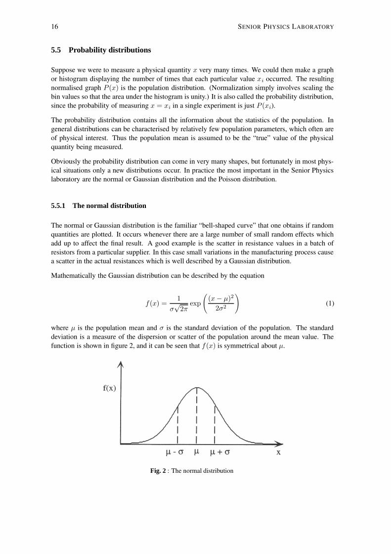
5.5 Probability distributions

Suppose we were to measure a physical quantity x very many times. We could then make a graphor histogram displaying the number of times that each particular value xi occurred. The resultingnormalised graph P (x) is the population distribution. (Normalization simply involves scaling thebin values so that the area under the histogram is unity.) It is also called the probability distribution,since the probability of measuring x = xi in a single experiment is just P (xi).

The probability distribution contains all the information about the statistics of the population. Ingeneral distributions can be characterised by relatively few population parameters, which often areof physical interest. Thus the population mean is assumed to be the “true” value of the physicalquantity being measured.

Obviously the probability distribution can come in very many shapes, but fortunately in most phys-ical situations only a new distributions occur. In practice the most important in the Senior Physicslaboratory are the normal or Gaussian distribution and the Poisson distribution.

5.5.1 The normal distribution

The normal or Gaussian distribution is the familiar “bell-shaped curve” that one obtains if randomquantities are plotted. It occurs whenever there are a large number of small random effects whichadd up to affect the final result. A good example is the scatter in resistance values in a batch ofresistors from a particular supplier. In this case small variations in the manufacturing process causea scatter in the actual resistances which is well described by a Gaussian distribution.

Mathematically the Gaussian distribution can be described by the equation

f(x) =1

σ√

2πexp

(

(x − µ)2

2σ2

)

(1)

where µ is the population mean and σ is the standard deviation of the population. The standarddeviation is a measure of the dispersion or scatter of the population around the mean value. Thefunction is shown in figure 2, and it can be seen that f(x) is symmetrical about µ.

Fig. 2 : The normal distribution


The probability of obtaining a result which lies between x and x + dx is f(x)dx, so the probabilitythat a measured value of x lies between x1 and x2 is found by integrating f(x) between the limits ofx1 and x2. In particular, for a normal distribution, the probability is 0.68 that a single measurementof x will lie within ±1σ of µ, while the probability is 0.95 (i.e. 20:1 on) that it will be within 2standard deviations of the mean. Table -1 gives the probability of obtaining a value of x betweenvarious limits and the expected number of occurrences for a random sample of 100 values.

Interval Probability Expectation (sample: 100)x1 x2

−∞ µ − 2σ 0.023 2µ − 2σ µ − σ 0.136 14µ − σ µ 0.341 34

µ µ + σ 0.341 34µ + σ µ + 2σ 0.136 14µ + 2σ +∞ 0.023 2−∞ +∞ 1.000 100

Table -1 : The Normal Distribution

5.5.2 The Poisson distribution

The Poisson distribution is the other probability distribution that you will need in the Senior PhysicsLaboratory. It describes situations in which discrete “events” can occur at random intervals. Forinstance, it allows us to determine the probability of obtaining a given number of radioactive decaysper second in a radioactive material, or a given number of telephone calls in one minute through anexchange, etc.

The Poisson distribution has only one parameter - the mean - and is given by the expression:

P (n) =1

n!µne−µ (2)

Note that P (n), unlike the normal distribution, is asymmetric or “skewed”. This is a natural con-sequence of the fact that n can never be negative. When the mean value is large, the Poissondistribution can be approximated by the normal distribution with mean µ and a standard deviation√

µ.

5.6 The statistics of data samples

Suppose that the results of a series of experimental observations are x1, x2, . . . , xn. The two mostimportant ’statistics’ for this set of data are the sample mean and sample standard deviation.

5.6.1 The sample mean

The sample mean x is just the familiar average value:


x =1

n

n∑

i=1

xi (3)

The sample mean x approximates to the true population mean but of course will not in general beequal to it, due to random noise.

5.6.2 The sample standard deviation

The sample standard deviation, s is a measure of the scatter of the observed data points around themeasured mean x. It is found from the formula:

s2 =1

n − 1

n∑

i=1

(xi − x)2 (4)

The quantity s2 is called the sample variance.

N.B. The sample standard deviation uses “n−1 weighting”, in the sense that (n−1) appears whereyou might have expected n. If you calculate s directly, you should use this formula; if you use acalculator with a standard deviation key, check to make sure that it uses (n − 1) weighting (manycalculators provide both n and n − 1 weighting). The reason for using n − 1 is that the samplemean appears on the right hand side of equation 4. The mean and standard deviation are thereforenot independent and this can be taken into account by reducing n by 1.

If your calculator does not have a standard deviation key, the following alternative formula may beeasier to use than equation 4:

(n − 1)s2 =∑

x2i −

1

n(∑

xi)2 (5)

The sample standard deviation is an approximation to the true population standard deviation. Thusif we were to take another measurement, very roughly we would expect it to be within ±s of x,68% of the time.

5.6.3 Standard error of the mean

Your observed sample mean x is itself a random variable, and an important statistical theorem statesthat it will have a normal distribution with a (population) mean and standard deviation σ/

√n. Thus

there is a 95% chance that x lies within ±2σ/√

n of the “actual” value, and it follows that we canimprove the precision of a result by increasing the number of data points n. The standard deviationof the sample is usually known, so it is quite common to estimate the precision of x by the standarderror of the mean:

E =s√n

=

(

∑

(xi − x)2

n(n − 1)

)1/2

(6)


For large values of n, E ≈ σ/√

n but for small data sets the standard error of the mean significantlyunderestimates the effects of random errors. A better way to estimate the precision of x is describedin the next section, but E is easy to calculate, and is often used to give a quick estimate of theprecision.

Exercises

1. A student measures a current with a nanoammeter. She obtains the following results: 6.1, 4.7,6.7, 5.4 and 6.0 nA. What are the mean, standard deviation and standard error of the mean?

[Ans: 5.8 nA, 0.8 nA, 0.3 nA]

2. The meter has an error of 2% FSD and readings were made on the 10 nA range. Will theoverall accuracy be improved significantly by taking further readings? Approximately howmany readings should she take?

[Ans: yes, 16]

5.7 Confidence intervals and statistical tests

We cannot, of course, exactly determine the population parameters from a small set of observations.We can, however, estimate the probability 1−α that a parameter lies within a particular range. Thisrange is called the 100(1 − α)% confidence interval. Thus α is the probability that the quantitylies outside the interval, and is often chosen to be 0.05 or 0.10 (corresponding to 95% and 90%confidence intervals).

5.7.1 The confidence interval for the mean

The confidence interval for the mean x is

x − s√n

(

tn−1;α

2

)

< µ < x +s√n

(

tn−1;α

2

)

(7)

which is usually abbreviated to

x ± E

(

tn−1;α

2

)

(8)

The quantity tm;α is known as Student’s1 t-distribution and can be regarded as a correction factorto the standard error E. The t-distribution tm;α is given in table -2. Note that t increases rapidlywhen we only have a few data points.

1“Student” was the nom-de-plume of W.S. Gossett, who introduced the t-distribution in 1908.


a/2 .25 .1 .05 .025 .01 .005m=n-1

1 1.000 3.078 6.314 12.706 31.821 63.6572 .816 1.886 2.920 4.303 6.965 9.9253 .765 1.638 2.353 3.182 4.541 5.8414 .741 1.533 2.132 2.776 3.747 4.604

5 .727 1.476 2.015 2.571 3.365 4.0326 .718 1.440 1.943 2.447 3.143 3.7077 .711 1.415 1.895 2.365 2.998 3.4998 .706 1.397 1.860 2.306 2.896 3.3559 .703 1.383 1.833 2.262 2.821 3.250

10 .700 1.372 1.812 2.228 2.764 3.16911 .697 1.363 1.796 2.201 2.718 3.10612 .695 1.356 1.782 2.179 2.681 3.05513 .694 1.350 1.771 2.160 2.650 3.01214 .692 1.345 1.761 2.145 2.624 2.977

15 .691 1.341 1.753 2.131 2.602 2.94716 .690 1.337 1.746 2.120 2.583 2.92117 .689 1.333 1.740 2.110 2.567 2.89818 .688 1.330 1.734 2.101 2.552 2.87819 .688 1.328 1.729 2.093 2.539 2.861

20 .687 1.325 1.725 2.086 2.528 2.84521 .686 1.323 1.721 2.080 2.518 2.83122 .686 1.321 1.717 2.074 2.508 2.81923 .685 1.319 1.714 2.069 2.500 2.80724 .685 1.318 1.711 2.064 2.492 2.797

25 .684 1.316 1.708 2.060 2.485 2.78726 .684 1.315 1.706 2.056 2.479 2.77927 .684 1.314 1.703 2.052 2.473 2.77128 .683 1.313 1.701 2.048 2.467 2.76329 .683 1.311 1.699 2.045 2.462 2.756

30 .683 1.310 1.697 2.042 2.457 2.75040 .681 1.303 1.684 2.021 2.423 2.70460 .679 1.296 1.671 2.000 2.390 2.660

120 .677 1.289 1.658 1.980 2.358 2.617∞ .674 1.282 1.645 1.960 2.326 2.576

Table -2 : Student’s t-distribution


Example

A student makes 4 independent determinations of the Rydberg constant for hydrogen using 4 linesof the Balmer series. The values obtained are:

1.097099 × 107 m−1

1.097046 × 107 m−1

1.097060 × 107 m−1

1.097107 × 107 m−1

What is the 95% confidence interval for the Rydberg constant?

From the data,

x = 1.097078 × 107 m−1 (9)s = 296.1 m−1

E = 148.0 m−1

For a 95% confidence interval, take α/2 = 0.025. From Table -2 we find t3;0.025 = 3.182. Hencethe 95% confidence interval is

x = (1.097078 ± 0.000047) × 107 m−1

5.7.2 The confidence interval for the standard deviation

Similarly, the confidence interval for the standard deviation can be calculated. It is

s

(

n − 1

χ2n−1;α/2

)1/2

< σ < s

(

n − 1

χ2n−1;−α/2

)1/2

(10)

Note that this interval is asymmetric. The quantity χ2m;α is called the χ2-distribution (χ is the Greek

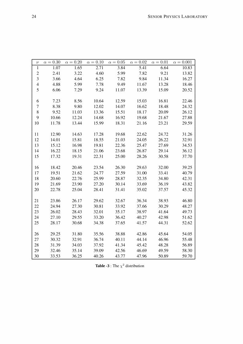
letter “chi”, pronounced KY to rhyme with MY and m = n − 1 is the degrees of freedom) and isgiven in table -3.

5.7.3 Statistical test

Most of the experiment notes in the Senior Physics Laboratory include a variation on the statement:

Compare your results with the theoretical value ....

We can turn such instructions into propositions or “hypotheses”:


My data are consistent with the theoretical value (YES or NO — cross out whicheverdoes not apply).

Because of the random errors which are present, we cannot state categorically that the results do/donot support the hypothesis, but often there are statistical tests which allow us to accept or rejectthe hypothesis with a certain level of significance. The level of significance, α, is defined to be theprobability that we mistakenly reject the hypothesis as false when in fact it is true. Obviously wewant α to be small and typically it is taken to be 0.05 or 0.10 (corresponding to 5% and 10% levelsof significance).

5.7.4 Tests for the mean and standard deviation

The proposition that the population mean (or standard deviation) equals a particular value X (or S)is easy to test. We accept the hypothesis that µ = X (or σ = S) at the α level of significance if Xor S lie in the confidence intervals given by equations 7 and 10 respectively.

The terminology can unfortunately be confusing! We use, for example, a 95% confidence intervalto test at the 5% level of significance (blame the statisticians!).

Example

Does the student’s data set in the example in section 5.7.1 agree with theory? The Rydberg constantfor hydrogen is known to be 1.09766 × 107 m−1. This lies outside of the confidence interval so wecan state that the data do not agree with theory at the 5% level of significance. There is clearly asystematic error present.

Other tests are not as straightforward. Two tests that are frequently needed are discussed in thefollowing sections.

5.7.5 Rejection of data

Students are quick to reject data points as “discrepant”. There are really only two ways of decidingwhether a dubious point should be discarded.

(a) Strong suspicion of systematic error. If the discrepant point is the only one your partner took,or if there is some other obvious problem (recorded, one hopes, in your log book), then youhave grounds for rejecting the data.

(b) Statistical testing. Let x and s be the mean and standard deviation of the n data points excludingthe possible discrepant point x′. Then x′ is discrepant at the 100α% level of significance andshould be rejected if the following inequality holds:

|x′ − x| > tn−1;α/2

(

n + 1

n

)1/2

s (11)

If equation 11 is not satisfied, x′ should be included with the other data.


5.7.6 The χ2 goodness-of-fit test

It is often necessary to decide whether our data have a particular probability distribution. Again wecannot say for sure, but can only indicate the probability that the data fit the distribution.

We must first construct some “test statistic” which measures the deviation of the data from thetheoretical distribution. If this test statistic is small we accept the hypothesis; otherwise we rejectit.

Suppose that we have a number of data points, which we can graph as a histogram or tabulate. Letoi be the number of points falling in the interval xi to xi+1 (o is for “observed”). We can alsocalculate the expected number ei for each interval using the theoretical distribution. For example,if the total number of points is 100 and we are testing a fit to the normal distribution, the numbersin table -3 can be used.

The test statistic is

χ2 =k∑

i=1

(ei − oi)2

ei(12)

where k is the total number of intervals.

Clearly if our data agree closely with the theoretical distribution χ2 will be small. Thus we acceptthe hypothesis that our data come from the distribution. Specifically, we accept the hypothesis atthe 100α level of significance if

χ2 < χ2ν;α (13)

where χ2ν;α is the χ2-distribution with ν = k − p − l “degrees of freedom” and

k = number of terms in the sum of equation 12p = number of parameters estimated from the data.

Tabulated values of χ2 as a function of ν and α are given in table -3.

Note that there is always a risk that equation 13 will not be satisfied when in fact the data do comefrom the theoretical distribution. For example, if we test at the 5% level of significance a series ofdata sets drawn at random form a normal distribution, we would expect 1 in 20 sets to give a valueof χ2 which violates equation 13.

The number p will change depending on the distribution and on how we define the distributionparameters. For example, if we wish to test our data to see if they fit to a normal distribution havinga mean and standard deviation equal to our measured x and s, then p = 2. If instead we want to testthe data to see if they come from a normal distribution with a given mean and standard deviation,then p = 0. For the Poisson distribution, if we take the mean equal to the observed mean, thenp = 1.

There is one important point to note. The test works only if all the ei are ≥ 5. If this is not the case,the data should be regrouped.


ν α = 0.30 α = 0.20 α = 0.10 α = 0.05 α = 0.02 α = 0.01 α = 0.001

1 1.07 1.65 2.71 3.84 5.41 6.64 10.832 2.41 3.22 4.60 5.99 7.82 9.21 13.823 3.66 4.64 6.25 7.82 9.84 11.34 16.274 4.88 5.99 7.78 9.49 11.67 13.28 18.465 6.06 7.29 9.24 11.07 13.39 15.09 20.52

6 7.23 8.56 10.64 12.59 15.03 16.81 22.467 8.38 9.80 12.02 14.07 16.62 18.48 24.328 9.52 11.03 13.36 15.51 18.17 20.09 26.129 10.66 12.24 14.68 16.92 19.68 21.67 27.88

10 11.78 13.44 15.99 18.31 21.16 23.21 29.59

11 12.90 14.63 17.28 19.68 22.62 24.72 31.2612 14.01 15.81 18.55 21.03 24.05 26.22 32.9113 15.12 16.98 19.81 22.36 25.47 27.69 34.5314 16.22 18.15 21.06 23.68 26.87 29.14 36.1215 17.32 19.31 22.31 25.00 28.26 30.58 37.70

16 18.42 20.46 23.54 26.30 29.63 32.00 39.2517 19.51 21.62 24.77 27.59 31.00 33.41 40.7918 20.60 22.76 25.99 28.87 32.35 34.80 42.3119 21.69 23.90 27.20 30.14 33.69 36.19 43.8220 22.78 25.04 28.41 31.41 35.02 37.57 45.32

21 23.86 26.17 29.62 32.67 36.34 38.93 46.8022 24.94 27.30 30.81 33.92 37.66 30.29 48.2723 26.02 28.43 32.01 35.17 38.97 41.64 49.7324 27.10 29.55 33.20 36.42 40.27 42.98 51.6225 28.17 30.68 34.38 37.65 41.57 44.31 52.62

26 29.25 31.80 35.56 38.88 42.86 45.64 54.0527 30.32 32.91 36.74 40.11 44.14 46.96 55.4828 31.39 34.03 37.92 41.34 45.42 48.28 56.8929 32.46 35.14 39.09 42.56 46.69 49.59 58.3030 33.53 36.25 40.26 43.77 47.96 50.89 59.70

Table -3 : The χ2 distribution


Example

A batch of 100 resistors is checked to see if the resistors are normal distributed. We use the χ2 testto see if the values are normally distributed with mean and standard deviation equal to the measuredvalues.

It is found that x = 10.22 kΩ and s = 0.29 kΩ. We group the data into the intervals (−∞, x− 2s), (x−2s, x− s), . . ., ( x+2s, +∞). The theoretically expected count in each interval can be obtainedfrom Table -3. The results are given below.

Interval Expected Observedcounts counts

xi xi + 1 ei oi (ei − oi)2/ei

−∞ x − 2s 14 16 16 0

x − 2s x − s 2

x − s x 34 31 0.265

x x + s 34 36 0.118

x + s x + 2s 14 16 17 0.0625

x + 2s ∞ 2

TOTAL: 100 100 0.445

Table -4 : Using the χ2 test

The number of degrees of freedom, ν, is 4 − 2 − 1 = 1 and from Table -3 the value of χ2 at the5% level of significance is 3.84. Note that the highest and lowest groups had to be combined withthe adjoining groups as they had fewer than 5 expected occurrences. The observed χ2 is less thanthe critical value of 3.84 so the data support the hypothesis that the resistors come from a normaldistribution.


5.8 Combining statistical errors

The rules for combining statistical errors are different from those we use when combining maximumerrors. Suppose for example we obtain a set of readings xi and yi which can be quoted in terms ofthe maximum errors as x±∆x, y ±∆y or in terms of the standard errors as x±Ex, y±Ey where

Ex =sx√nx

Ey =sy√ny

The absolute maximum error in f = x + y is ∆f = ∆x + ∆y. The standard error in f is given by

Ef = (E2x + E2

y)1/2 (14)

This procedure for combining errors can also be applied to maximum errors to obtain a more re-alistic estimate of the maximum error in f . In either case, the quadratic combination of errors isvalid only if Ex, Ey (or ∆x, ∆x) are independent. The following table summarises the rules forcombining standard errors.

Function f Standard Error in f

f = x + yf = x − y

Ef = (E2x + E2

y)1/2

f = xyf = x/y

Ef

f =

[

(

Ex

x

)2+(

Ey

y

)2]1/2

f = xn Ef

f = |n|(

Ex

x

)

Since these rules apply only when the errors in x are independent of the errors in y, it may benecessary to arrange the formula for f before hand so that it only contains quantities whose errorsare independent.

Example

Measurements of voltage (V ) and current (I) are used to calculate resistance (R) and power (P ).Errors in V do not depend on errors in I . We find

R =V

I

andER

R=

[

(

EV

V

)2

+

(

EI

I

)2]1/2

We cannot use P = RI2 since the error in R depends on the error in I . Rather, we use P = V I;thus the fractional error in P is the same as the fractional error in R.


5.9 Errors and graphs

A problem which arises frequently in experimental work is to determine the relationship betweentwo quantities, say y and x. By plotting y vs x on a linear, log or log-linear graph we can check forexample if y = ax − b or y = axn or y = aebx and obtain an estimate for the constants a and b bydrawing a line of best fit through the experimental points. This line tends to average out the errorsin each individual point. If we wish to determine the worst possible error in the slope of a graph,we can also draw lines of worst fit through the error bars associated with each point. Care should betaken, however, to ensure that the worst fit lines pass through all points (including y = 0, x = 0 ifwe have good reason to believe that they should). Plots of voltage vs current, for example, usually(but not always) pass through (0, 0).

It should be noted that worst fit curves usually overestimate the actual error in the slope of a graphand that a so-called line of “best fit” drawn by eye may have significantly different slopes whendrawn by different observers. Both of these limitations can be overcome by the regression tech-niques outlined below.

If random errors dominate, then the method of least squares can be used to estimate the line of bestfit.

5.9.1 The method of least squares

Suppose y1, y2, . . . yn are the values of a measured quantity y corresponding to values x1, x2, . . . xn

of another quantity x. For these data, we wish to determine the “best fit” line of the form

y = ax + b (15)

The usual ways is, of course, to estimate by eye the best line and draw it in with a ruler. If the datapoints lie very close to a straight line this method is as good as any, but if there are large errors it isdifficult to estimate a “best” line, and different lines will be drawn by different experimenters.

The method of least squares provides an unambiguous way of choosing the best line. It is themethod used by Excel and Origin. Suppose we fit the data by a line of the form of equation 15.Then for each data point there will be a small error

∆ = yi − (axi + b) (16)

between the line and the actual measured values of y.

An estimate of how well the line fits the data is given by the sum of squares S:

S =∑

[yi − (axi + b)]2 (17)

The line of best fit, by definition, is the one that minimises S. As S is a function of the slope, a, andintercept, b, we can find the minimum of S by differentiating with respect to a and b and setting thederivatives equal to 0:


∂S

∂a= 2

∑

xi(axi + b − yi) = 0 (18)

and

∂S

∂b= 2

∑

(axi + b − yi) = 0 (19)

Solving for a and b gives:

a =n∑

xiyi −∑

xi∑

yi

n∑

x2i − (

∑

xi)2(20)

and

b =

∑

yi∑

x2i −

∑

xi∑

xiyi

n∑

x2i − (

∑

xi)2(21)

Exercises

1. The following voltage and current readings were obtained for a particular device. Obtain thebest fit line (a) by eye and (b) by the least squares method, and hence estimate the resistanceof the device.Note that the least squares line does not pass through (0, 0).[Ans: a = 1.02, b = −0.03]

2. How can we change the above formulae to ensure that the line does pass through (0, 0)? Showthat in that case,

a =

∑

xiyi∑

x2i

and hence find a.[Ans: a = 1.007]

3. Show by the method of least squares that the best fit of a series of n readings y1, y2, . . . yn tothe function y = k (where k is a constant) is given by k = y.

4. Show that the best fit line of the form y = ax + b passes through the point (x, y).

5.9.2 Confidence intervals for the slope and intercept

One advantage of the least squares method is that it can provide reasonable estimates for the uncer-tainty in the slope and intercept of the line of best fit. This is difficult to do by the “eyeball” methodof best and worst fit lines. The 100(1 − α)% confidence intervals for the slope and intercept aregiven by the following formulae:


a ± (tn−2;α/2)Ea (22)

and

b ± (tn−2;α/2)Ea

(

∑

x2i

n

)1/2

(23)

whereE2

a =(n∑

[yi − axi + b])2

(n − 2)[n∑

x2i − (

∑

xi)2](24)

Note that the t-distribution is taken with n − 2 degrees of freedom; this is because we know havetwo dependent or derived quantities (a and b).

The errors in a and b can usually be treated like any other errors. They are not independent, however,and if you need to calculate a function f(a, b) which includes both quantities, care must be taken.When Origin is used for fitting a least squares line to data it automatically calculates errors for theslope and intercept.

5.9.3 A word of warning

The method of least squares is essentially a mathematical black box: put data in and it will producethe numbers a and b. The results may be complete nonsense, however, and it is always necessaryto graph your data and draw in the least squares line. If the fit looks plausible by eye, then there isprobably no difficulty. If the line is clearly wrong, then the method should not be used. The leastsquares technique can fail for several reasons:

• The data do not fit a straight line. A quadratic curve or some other shape may be moreappropriate.

• The independent variable (x) may have significant errors. The least squares method assumesthat all the error is associated with the dependent variable y.

• The scatter is not uniform along the line. The method is based on the assumption that y isdistributed as a normal random variable about the line, with a constant standard deviation.This may not be true, especially if the fit is to a power law and the data have been plotted onlog-log axes to give a linear relation.

Exercise

Suppose y ranges from 0.1 to 100, and has a standard deviation over this range of 0.05. Using logpaper, draw in the ±s error bars for y = 0.1, 1, 10 and 100.


5.10 Slopes and intercepts

A straight line can be fitted to linear, power law or exponential curves provided the appropriatelinear or logarithmic graph paper is used. Regardless of the type of curve plotted, the slope of thestraight line y = ax + b is given by a = ∆y/∆x. The value of other constants can be found bysubstitution. Figure 3 shows several examples.

Fig. 3 : Calculating the slopes of straight lines


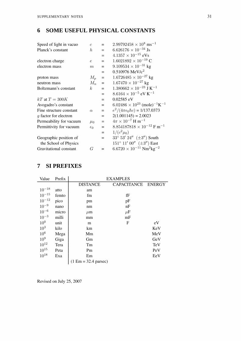
6 SOME USEFUL PHYSICAL CONSTANTS

Speed of light in vacuo c = 2.99792458 × 108 ms−1

Planck’s constant h = 6.626176 × 10−34 Js= 4.1357 × 10−15 eVs

electron charge e = 1.6021892 × 10−19 Celectron mass m = 9.109534 × 10−31 kg

= 0.510976 MeV/c2

proton mass Mp = 1.6726485 × 10−27 kgneutron mass Mn = 1.67470 × 10−27 kgBoltzmann’s constant k = 1.380662 × 10−23 J K−1

= 8.6164 × 10−5 eV K−1

kT at T = 300K = 0.02585 eVAvogadro’s constant = 6.02486 × 1023 (mole)−1K−1

Fine structure constant α = e2/(4πε0hc) = 1/137.0373g factor for electron = 2(1.001145) = 2.0023Permeability for vacuum µ0 = 4π × 10−7 H m−1

Permittivity for vacuum ε0 = 8.854187818 × 10−12 F m−1

= 1/(c2µ0)Geographic position of = 33 53′ 24′′ (±3′′) South

the School of Physics 151 11′ 00′′ (±3′′) EastGravitational constant G = 6.6720 × 10−11 Nm2kg−2

7 SI PREFIXES

Value Prefix EXAMPLESDISTANCE CAPACITANCE ENERGY

10−18 atto am10−15 femto fm fF10−12 pico pm pF10−9 nano nm nF10−6 micro µm µF10−3 milli mm mF100 unit m F eV103 kilo km KeV106 Mega Mm MeV109 Giga Gm GeV1012 Tera Tm TeV1015 Peta Pm PeV1018 Exa Em EeV

(1 Em = 32.4 parsec)

Revised on July 25, 2007

university of sydney school of physics...

Documents