university of ottawa faculty of graduate and post-doctoral studies...
TRANSCRIPT

M.Sc. in System Science, University of Ottawa Sara Barghi
University of Ottawa
Faculty of Graduate and Post-Doctoral Studies
Master's Program in Systems Science
Thesis Title:
Water Management Modeling in the Simulation of Water Systems in Coastal Communities
Student Name: Sara Barghi
Thesis Supervisors:
Professors Daniel E. Lane and John D. Clarke
Telfer School of Management
University of Ottawa
©Sara Barghi, Ottawa, Canada, 2013

M.Sc. in System Science, University of Ottawa Sara Barghi
ii
Abstract
It is no longer a question of scientific debate that research declares our climate is changing.
One of the most important and visible impacts of this phenomenon is sea level rise which
has impacts on coastal cities and island communities. Sea level rise also magnifies storm
surges which can have severely damaging impacts on different human made infrastructure
facilities near the shorelines in coastal zones. In this research we are concerned about the
proximity of water systems as one of the most vulnerable infrastructures in the coastal zones
because of the impact of stormwater combining with sewage water. In Canada, the
government has plans to address these issues, but to date, there needs to be further attention
to stormwater management in coastal zones across the country. This research discusses the
impacts of severe environmental events, e.g., hurricanes and storm surge, on the water
systems of selected coastal communities in Canada. The purpose of this research is to model
coastal zone water systems using the open source StormWater Management Modelling
(SWMM) software in order to manage stormwater and system response to storms and storm
surge on water treatment plants in these areas. Arichat on Isle Madame, Cape Breton, one of
the most sensitive coastal zones in Canada, is the focal point case studies for this research as
part of the C-Change International Community-University Research Alliance (ICURA)
2009-2015 project.
Keywords: Climate change, sea level rise, stormwater, water systems

M.Sc. in System Science, University of Ottawa Sara Barghi
iii
Acknowledgements
Formest, I would like to express my immense gratitude to my supervisor, Professor Daniel
Lane, for his continuous support for my Master’s studies and research. His helpful
knowledge, motivation, patience and wonderful personality made this journey easier and
sweeter for me. This work would not have been possible without his help. Working with him
was one of the most wonderful experiences that I have ever had.
Besides my supervisor, I would like to thank Municipality of Richmond County people,
specifically Chris Boudreau for his help in data gathering for this research, which made the
path of the research smoother for me.
Also, I would like to thank the C-Change group, especially my Co-supervisor Mr. John
Clarke and Dr. Colleen Mercer-Clarke for their insightful comments, immense knowledge
and willing to spread their knowledge kindly and supportively. Also, I would like to thank
Kathy Cunningham for always being there for my time to time questions and requests.
It was my pleasure to be a part of the Systems Science program at University of Ottawa and
I would like to thank all the professors and staffs in this program and university.
Specifically, I thank Ms. Monique Walker for her unsparing help during my studies in this
program.
Last but not the least, I would like to thank my family and friends, for which I really cannot
find a word to express my gratitude and thankfulness for their tremendous support. My
parents who were always supportive from the moment I entered this world; my siblings who
were always there for me and did whatever they could to help me find my way in life. I have
to especially thank my dearest husband, Mohammad, whose endless love and
encouragement was a glamorous energy for me to continue my way.

M.Sc. in System Science, University of Ottawa Sara Barghi
iv
Table of Contents
ABSTRACT .................................................................................................................................................. II
ACKNOWLEDGEMENTS ............................................................................................................................. III
TABLE OF CONTENTS ................................................................................................................................. IV
LIST OF FIGURES ....................................................................................................................................... VII
LIST OF TABLES ........................................................................................................................................... X
GLOSSARY ............................................................................................................................................... XIX
1. INTRODUCTION ............................................................................................................................. 1
1.1. MOTIVATION / PROBLEM DEFINITION ............................................................................................................ 1 1.2. RESEARCH QUESTIONS AND OBJECTIVES .......................................................................................................... 6 1.3. PLAN OF THE THESIS ................................................................................................................................... 6
2. LITERATURE REVIEW .................................................................................................................. 8
2.1. WATER AND CLIMATE CHANGE .......................................................................................................................... 8 2.2. COASTAL COMMUNITIES .............................................................................................................................. 9 2.3. WATER INFRASTRUCTURE MODELLING ......................................................................................................... 10
2.3.1. SWWM5.0 as a Simulation Tool in Stormwater Management ................................................... 14 2.4. APPLICATIONS ......................................................................................................................................... 15
3. METHODOLOGY ........................................................................................................................... 18
3.1. MODELING WITH SWMM .............................................................................................................................. 18 3.2. PHYSICAL COMPONENTS IN SWMM ........................................................................................................... 19 3.3. SWMM SETTINGS AND INPUTS .................................................................................................................. 29 3.4. OUTPUTS İN SWMM ............................................................................................................................... 35 3.5. PROCESS OF RESEARCH.............................................................................................................................. 36
4. RESEARCH PROCESS ................................................................................................................... 39
4.1. MODELING THE ARICHAT WATER SYSTEM USING THE SWMM MODELING SYSTEM ............................................. 39 4.1.1. Arichat Map ................................................................................................................................. 39 4.1.2. Model Subcatchments ................................................................................................................. 40 4.1.3. Arichat Map Geo-referencing ...................................................................................................... 42 4.1.4. Subcatchment Impervious Characteristics .................................................................................. 43 4.1.5. Water Quality and Common Pollutants ...................................................................................... 43 4.1.6. Land Use ...................................................................................................................................... 43 4.1.7. Model Junctions and Storage Units ............................................................................................. 44 4.1.8. Model Conduits ........................................................................................................................... 48 4.1.9. Pumps .......................................................................................................................................... 48 4.1.10. Regulators ................................................................................................................................... 50 4.1.11. Outfalls ........................................................................................................................................ 53
4.2. ARICHAT HYDROLOGIC SETTINGS AND INPUTS FOR APPLYING DIFFERENT SCENARIOS IN SWMM ............................ 55

M.Sc. in System Science, University of Ottawa Sara Barghi
v
4.2.1. Controllable variables: Regulators .............................................................................................. 55 4.2.2. Uncontrollable variables ............................................................................................................. 56
4.2.2.1. Precipitation ........................................................................................................................................... 56 4.2.2.2. Tidal level ................................................................................................................................................ 59 4.2.2.3. Initial Depth ............................................................................................................................................ 65 4.2.2.4. Impervious Percentage ........................................................................................................................... 65
5. RESULTS AND ANALYSIS ............................................................................................................ 66
5.1. SIMULATION DESIGN ...................................................................................................................................... 66 5.1.1. Status Quo Scenario .......................................................................................................................... 66 5.1.2. Best Case Scenario ............................................................................................................................ 68 5.1.3. Worst Case Scenario .......................................................................................................................... 69 5.1.4. Precipitation Focus Scenario ............................................................................................................. 69 5.1.5. Tide Focus Scenario ........................................................................................................................... 70 5.1.6. Tidal Level and Initial Depth Focus Scenario ..................................................................................... 70 5.1.7. Regulators and Precipitation Focus Scenario .................................................................................... 70 5.1.8. Tidal Level and Impervious Percentage Focus Scenario .................................................................... 71 5.1.9. Initial Depth and Precipitation Focus Scenario .................................................................................. 71 5.1.10. Initial Depth and Impervious Percentage Focus Scenario ............................................................... 71
5.2. SCENARIO RESULTS ................................................................................................................................... 72 5.2.1. Status Quo Scenario Results ........................................................................................................ 72 5.2.2. Best Case Scenario Results .......................................................................................................... 77 5.2.3. Worst Case Scenario Results ....................................................................................................... 82 5.2.4. Precipitation Focus Scenario Results ........................................................................................... 87 5.2.5. Tide Focus Scenario Results ......................................................................................................... 91 5.2.6. Tide and Initial Depth Focus Scenario Results ............................................................................. 94 5.2.7. Regulators and Precipitation Focus Scenario Results .................................................................. 97 5.2.8. Tide and Impervious Focus Scenario Results ............................................................................. 100 5.2.9. Initial Depth and Precipitation Focus Scenario Results ............................................................. 102 5.2.10. Initial Depth and Impervious Percentage Focus Scenario Results ............................................. 108
5.3 ANALYSIS OF THE RESULTS .............................................................................................................................. 110
6. CONCLUSION, SUGGESTIONS AND RECOMMENDATIONS FOR FUTURE STUDY .......... 115
6.1. SUMMARY OF RESULTS ................................................................................................................................. 115 6.2. CONCLUSIONS AND SUGGESTIONS FOR IMPROVEMENT OF THE WATER SYSTEM IN ARICHAT .................................. 116
6.2.1. Pump P1 Performance ............................................................................................................... 116 6.2.2. Junction j11 Capacity ................................................................................................................. 117 6.2.3. Junctions j6 and j8 Capacities .................................................................................................... 117 6.2.4. Treatment Plant Capacity .......................................................................................................... 117
6.3. RECOMMENDATIONS FOR FUTURE STUDY ........................................................................................................ 118 6.3.1 Data .................................................................................................................................................. 118 6.3.2 Water Quality ................................................................................................................................... 118 6.3.3. Application to Other Coastal Communities ..................................................................................... 119
7. BIBLIOGRAPHY .......................................................................................................................... 120
APPENDIX A ........................................................................................................................................ 124

M.Sc. in System Science, University of Ottawa Sara Barghi
vi
APPENDİX B ........................................................................................................................................ 125
APPENDİX C ........................................................................................................................................ 127
C.1. STATUS QUO SCENARIO SIMULATION STATUS REPORT ....................................................................................... 127 C.2. BEST CASE SCENARIO SIMULATION STATUS REPORT ........................................................................................... 137 C.3. WORST CASE SCENARIO SIMULATION STATUS REPORT ....................................................................................... 147 C.4. PRECIPITATION FOCUS SCENARIO SIMULATION STATUS REPORT ........................................................................... 158 C.5. TIDE FOCUS SCENARIO SIMULATION STATUS REPORT ......................................................................................... 169 C.6. TIDE AND INITIAL DEPTH FOCUS SCENARIO SIMULATION STATUS REPORT............................................................... 180 C.7. REGULATORS AND PRECIPITATION FOCUS SCENARIO SIMULATION STATUS REPORT .................................................. 191 C.8. TIDE AND IMPERVIOUS FOCUS SCENARIO SIMULATION STATUS REPORT ................................................................. 202 C.9. DEPTH AND PRECIPITATION FOCUS SCENARIO SIMULATION STATUS REPORT ........................................................... 213 C.10. INITIAL DEPTH AND IMPERVIOUS FOCUS SCENARIO SIMULATION STATUS REPORT .................................................. 224

M.Sc. in System Science, University of Ottawa Sara Barghi
vii
List of Figures
Figure 2.1.The connections between human activities, climate change and water resources . 8
Figure 2.2. Municipal Stormwater Management System ...................................................... 11
Figure 2.3. Isle Madamee map noting the village of Arichat along the southern shore ........ 16
Figure 3.1. Junction-Conduits representation in SWMM ...................................................... 20
Figure 3.2. Representation of Isle Madamee model subcatchment Area, S3 in SWMM ...... 20
Figure 3.3. SWMM representation of Isle Madamee model subcatchment S3 linked to
junction j3 which is connected to storage unit j10 through conduit c7 ................................. 22
Figure 3.4. Type 1 pump curve .............................................................................................. 23
Figure 3.5. Type 2 pump curve .............................................................................................. 24
Figure 3.6. Type 3 pump curve .............................................................................................. 24
Figure 3.7. Type 4 pump curve .............................................................................................. 25
Figure 3.8. SWMM representation of Isle Madamee model subcatchment S3 linked to
junction j3 which is connected to junction j10 through conduit c7 and pump p3 linked to
junction j11 ............................................................................................................................ 25
Figure 3.9. SWMM representation of Isle Madamee model subcatchment S3 linked to
junction j3 connected to junction j10 through conduit c7 and pump p3 linked to junction j11.
J10 connected to outfall (Outfall3) and associated control regulator (R3) in SWMM ......... 26
Figure 3.10. Geographical map of Arichat used as the backdrop image of the model Isle
Madame water system model in SWMM .............................................................................. 28
Figure 3.11. Rain gauge representation in SWMM ............................................................... 31
Figure 4.1. Arichat model's backdrop image (Arichat map) ................................................. 40
Figure 4.2. Arichat water system model in SWMM with subcatchments S1 to S13 indicated
............................................................................................................................................... 41
Figure 4.3. A sample pump, p3, performance curve ............................................................. 49
Figure 4.4. Arichat developed model with related pictures-part 1 ........................................ 51
Figure 4.5. Arichat developed model with related pictures-part 2 ........................................ 52
Figure 4.6. Second precipitation case “P1”: The historical data for the 24-hour period with
the maximum precipitation. Total maximum rainfall for overall precipitation is 86mm ...... 58
Figure 4.7. Tidal level case number 1: Historical highest high level tide ............................. 59

M.Sc. in System Science, University of Ottawa Sara Barghi
viii
Figure 4.8. Tidal level case number (ii): Historical lowest low level tide ............................. 61
Figure 4.9. “Mean/Lowfirst” tidal alternative ....................................................................... 62
Figure 4.10. “Mean/Highfirst” tidal alternative ..................................................................... 64
Figure 5.1.Outfalls Depth ...................................................................................................... 74
Figure 5.2. TSS values in Outfall2, Outfall3 and TPO .......................................................... 75
Figure 5.3. System Total Inflow and Outflow for SQ Scenario ............................................ 76
Figure 5.4. Outfall Depths for Best Case Scenario ................................................................ 79
Figure 5.5. System Runoff for the Best Case Scenario ......................................................... 80
Figure 5.6. System Total Inflow and Outflow for the Best Case Scenario ........................... 81
Figure 5.7. Storage Units Depth in Worst Case Scenario ...................................................... 84
Figure 5.8. Pumps Outlet Junctions and Treatment Plant Depth in Worst Case Scenario .... 84
Figure 5.9. Outfall Depths in Worst Case Scenario ............................................................... 85
Figure 5.10. System Total Inflow and Outflow in the Precipitation Focus Scenario ............ 88
Figure 5.11. System Flooding for the Precipitation Focus Scenario ..................................... 89
Figure 5.12. Profile plot for the Lower Road Connections from j6 to j15 at 3:15:00 for
Precipitation Focus Scenario ................................................................................................. 90
Figure 5.13. Outfall Depth for Tide Focus Scenario ............................................................. 92
Table 5.14. High Road Junctions’ Depth in the Tide and Initial Depth Focus Scenario ....... 95
Figure 5.15. System Flooding in the Tide and Initial Depth Focus Scenario ........................ 96
Figure 5.16. System Flooding in the Regulators and Precipitation Focus Scenario .............. 99
Figure 5.17. System Total Inflow and Outflow for the Regulators and Precipitation Focus
Scenario ............................................................................................................................... 100
Figure 5.18.Summary of Results for the Tide and Impervious Focus Scenario .................. 101
Figure 5.19. System Total inflow and Outflow for the Initial Depth and Precipitation Focus
Scenario ............................................................................................................................... 104
Figure 5.20. Junctions Flooding Summary for the Initial Depth and Precipitation Focus
Scenario ............................................................................................................................... 105
Figure 5.21. Profile plot for the Lower Road Connections from j6 to j15 at 3:00:00 for Initial
Depth and Precipitation Focus Scenario .............................................................................. 106
Figure 5.22. Junction j8 Depth in the Simulation of the Initial Depth and Precipitation Focus
Scenario ............................................................................................................................... 107

M.Sc. in System Science, University of Ottawa Sara Barghi
ix
Figure 5.23. System Flooding for the Initial Depth and Impervious Focus Scenario ......... 109
Figure A.1. Maximum monthly average precipitation histogram excluding 0mm to 1mm
precipitation ......................................................................................................................... 124
Figure A.2. Minimum Monthly average precipitation precipitation histogram excluding
0mm to 1mm precipitation ................................................................................................... 124

M.Sc. in System Science, University of Ottawa Sara Barghi
x
List of Tables
Table 3.1. Typical EMC’s for selected pollutants ................................................................. 33
Table 4.1. Sample subcatchment properties:S3 ..................................................................... 41
Table 4.2.Hand held GPS data used for the simulation ......................................................... 46
Table 4.3. RTK survey and hand held GPS elevations and their relative elevations ............ 47
Table 4.4. Model Sample junction properties: j11 ................................................................ 47
Table 4.5. Sample storage unit properties: j10 ...................................................................... 47
Table 4.6. Sample conduit properties: c7 .............................................................................. 48
Table 4.7. Sample pumps properties: p3 ............................................................................... 49
Table 4.8. Sample regulators properties: R3 ......................................................................... 53
Table 4.9. Sample outfall properties: Outfall3 ...................................................................... 54
Table 4.10. Monthly average precipitation for the seven-year data set, 2004 to 2011 .......... 56
Table 4.11.Second precipitation case “P1” :The historical data for the 24-hour with the
maximum precipitation with 86mm for overall precipitation ................................................ 58
Table 4.12. Tidal level case number (i): Historical highest high level tide ........................... 60
Table 4.13. Tidal level case number (ii): Historical lowest low level tide ............................ 61
Table 4.14. “Mean/Lowfirst” tidal alternative ....................................................................... 63
Table 4.15. ”Mean/Highfirst” tidal alternative ...................................................................... 64
Table 5.1. Simulation design:Scenarioes description ............................................................ 67
Table 5.2. Status Quo Scenario Simulation Results Summary .............................................. 77
Table 5.3. Best Case Scenario Result Summary .................................................................... 81
Table 5.4. Worst Case Scenario Results Summary ............................................................... 87
Table 5.5. Precipitation Focus Scenario Results Summary ................................................... 91
Table 5.6. Summary of Results for Tide Focus Scenario ...................................................... 93
Table 5.7. Tide and Initial Depth Focus Scenario Results Summary .................................... 97
Table 5.8. Regulators and Precipitation Focus Scenario Results Summary ........................ 100
Table 5.9. Summary of Results in the Tide and Impervious Focus Scenario ...................... 102
Table 5.10. Summary of Results in the Depth and Precipitation Focus Scenario ............... 107
Table 5.11. Summary of Results for the Initial Depth and Impervious Percentage Focus
Scenario ............................................................................................................................... 110

M.Sc. in System Science, University of Ottawa Sara Barghi
xi
Table 5.12. Results summary for scenario 1 to 10 .............................................................. 111
Table 5.13. Flooding Summary for Junctions Flooded in Scenario 1 to 10 ........................ 112
Table 5.14. Surcharging Summary for Junctions surcharged in Scenario 1 to 10 ............... 113
Table 5.15. Utilization Percentage for Pumps 1 to 5 in the Scenarios 1 to 10 .................... 114
Table C.1. Analysis Options: SQ Scenario ......................................................................... 127
Table C.2. Runoff Quantity Continuity: SQ Scenario ......................................................... 127
Table C.3. Runoff Quality Continuity: SQ Scenario ........................................................... 128
Table C.4. Flow Routing Continuity: SQ Scenario ............................................................. 128
Table C.5. Quality Routing Continuity: SQ Scenario ......................................................... 129
Table C.6. Highest Continuity Errors: SQ Scenario ............................................................ 129
Table C.7. Time-Step Critical Elements: SQ Scenario ........................................................ 129
Table C.8. Highest Flow Instability Indexes: SQ Scenario ................................................. 129
Table C.9. Routing Time Step Summary: SQ Scenario ...................................................... 130
Table C.10. Subcatchment Runoff Summary: SQ Scenario ................................................ 130
Table C.11. Subcatchment Washoff Summary: SQ Scenario ............................................. 131
Table C.12. Node Depth Summary: SQ Scenario .............................................................. 132
Table C.13. Node Inflow Summary: SQ Scenario .............................................................. 133
Table C.14. Node Surcharge Summary: SQ Scenario ......................................................... 133
Table C.15. Node Flooding Summary: SQ Scenario ........................................................... 133
Table C.16. Storage Volume Summary: SQ Scenario ......................................................... 134
Table C.17. Outfall Loading Summary: SQ Scenario ......................................................... 134
Table C.18. Link Flow Summary: SQ Scenario .................................................................. 135
Table C.19. Flow Classification Summary: SQ Scenario .................................................... 136
Table C.20. Conduit Surcharge Summary: SQ Scenario ..................................................... 136
Table C.21. Pumping Summary: SQ Scenario .................................................................... 137
Table C.22. Analysis Options: Best Case Scenario ............................................................. 137
Table C.23. Runoff Quantity Continuity: Best Case Scenario ............................................ 138
Table C.24. Runoff Quality Continuity: Best Case Scenario .............................................. 138
Table C.25. Flow Routing Continuity: Best Case Scenario ............................................... 139
Table C.26. Quality Routing Continuity: Best Case Scenario ............................................. 139
Table C.27. Highest Continuity Errors: Best Case Scenario ............................................... 139

M.Sc. in System Science, University of Ottawa Sara Barghi
xii
Table C.28. Time-Step Critical Elements: Best Case Scenario ........................................... 140
Table C.29. Highest Flow Instability Indexes: Best Case Scenario .................................... 140
Table C.30. Routing Time Step Summary: Best Case Scenario .......................................... 140
Table C.31. Subcatchment Runoff Summary: Best Case Scenario ..................................... 140
Table C.32. Subcatchment Washoff Summary: Best Case Scenario ................................... 141
Table C.33. Node Depth Summary: Best Case Scenario ..................................................... 142
Table C.34. Node Inflow Summary: Best Case Scenario .................................................... 143
Table C.35. Node Surcharge Summary: Best Case Scenario .............................................. 143
Table C.36. Node Flooding Summary: Best Case Scenario ................................................ 143
Table C.37. Storage Volume Summary: Best Case Scenario .............................................. 144
Table C.38. Outfall Loading Summary: Best Case Scenario .............................................. 144
Table C.39. Link Flow Summary: Best Case Scenario ....................................................... 145
Table C.40. Flow Classification Summary: Best Case Scenario ........................................ 146
Table C.41. Conduit Surcharge Summary: Best Case Scenario .......................................... 146
Table C.42. Pumping Summary: Best Case Scenario .......................................................... 147
Table C.43. Analysis Options: Worst Case Scenario .......................................................... 147
Table C.44. Runoff Quantity Continuity: Worst Case Scenario ......................................... 148
Table C.45. Runoff Quality Continuity: Worst Case Scenario ........................................... 148
Table C.46. Flow Routing Continuity: Worst Case Scenario .............................................. 149
Table C.47. Quality Routing Continuity: Worst Case Scenario .......................................... 149
Table C.48. Highest Continuity Errors: Worst Case Scenario ............................................ 149
Table C.49. Time-Step Critical Elements: Worst Case Scenario ........................................ 150
Table C.50. Highest Flow Instability Indexes: Worst Case Scenario .................................. 150
Table C.51. Routing Time Step Summary: Worst Case Scenario ....................................... 150
Table C.52. Subcatchment Runoff Summary: Worst Case Scenario .................................. 151
Table C.53. Subcatchment Washoff Summary: Worst Case Scenario ................................ 151
Table C.54. Node Depth Summary: Worst Case Scenario .................................................. 152
Table C.55. Node Inflow Summary: Worst Case Scenario ................................................. 153
Table C.56. Node Surcharge Summary: Worst Case Scenario ........................................... 154
Table C.57. Node Flooding Summary: Worst Case Scenario ............................................. 154
Table C.58. Storage Volume Summary: Worst Case Scenario ........................................... 155

M.Sc. in System Science, University of Ottawa Sara Barghi
xiii
Table C.59. Outfall Loading Summary: Worst Case Scenario ............................................ 155
Table C.60. Link Flow Summary: Worst Case Scenario ..................................................... 156
Table C.61. Flow Classification Summary: Worst Case Scenario ...................................... 157
Table C.62. Conduit Surcharge Summary: Worst Case Scenario ...................................... 157
Table C.63. Pumping Summary: Worst Case Scenario ....................................................... 158
Table C.64. Analysis Options: Precipitation Focus Scenario .............................................. 158
Table C.65. Runoff Quantity Continuity: Precipitation Focus Scenario ............................. 159
Table C.66. Runoff Quality Continuity: Precipitation Focus Scenario ............................... 159
Table C.67. Flow Routing Continuity: Precipitation Focus Scenario ................................. 160
Table C.68. Quality Routing Continuity: Precipitation Focus Scenario ............................. 160
Table C.69. Time-Step Critical Elements: Precipitation Focus Scenario ............................ 160
Table C.70. Highest Flow Instability Indexes: Precipitation Focus Scenario ..................... 161
Table C.71. Routing Time Step Summary: Precipitation Focus Scenario .......................... 161
Table C.72. Subcatchment Runoff Summary: Precipitation Focus Scenario ...................... 161
Table C.73. Subcatchment Washoff Summary: Precipitation Focus Scenario ................... 162
Table C.74. Node Depth Summary: Precipitation Focus Scenario ..................................... 163
Table C.75. Node Inflow Summary: Precipitation Focus Scenario ..................................... 164
Table C.76. Node Surcharge Summary: Precipitation Focus Scenario ............................... 165
Table C.77. Node Flooding Summary: Precipitation Focus Scenario ................................. 165
Table C.78. Storage Volume Summary: Precipitation Focus Scenario ............................... 166
Table C.79. Outfall Loading Summary: Precipitation Focus Scenario ............................... 166
Table C.80. Link Flow Summary: Precipitation Focus Scenario ........................................ 167
Table C.81. Flow Classification Summary: Precipitation Focus Scenario .......................... 168
Table C.82. Conduit Surcharge Summary: Precipitation Focus Scenario ........................... 168
Table C.83. Pumping Summary: Precipitation Focus Scenario .......................................... 169
Table C.84. Analysis Options: Tide Focus Scenario ........................................................... 169
Table C.85. Runoff Quantity Continuity: Tide Focus Scenario .......................................... 170
Table C.86. Runoff Quality Continuity: Precipitation Focus Scenario ............................... 170
Table C.87. Flow Routing Continuity: Precipitation Focus Scenario ................................. 171
Table C.88. Quality Routing Continuity: Precipitation Focus Scenario ............................. 171
Table C.89. Highest Continuity Errors: Tide Focus Scenario ............................................. 172

M.Sc. in System Science, University of Ottawa Sara Barghi
xiv
Table C.90. Time-Step Critical Elements: Tide Focus Scenario ......................................... 172
Table C.91. Highest Flow Instability Indexes: Tide Focus Scenario .................................. 172
Table C.92. Routing Time Step Summary: Tide Focus Scenario ........................................ 172
Table C.93. Subcatchment Runoff Summary: Tide Focus Scenario ................................... 173
Table C.94. Subcatchment Washoff Summary: Tide Focus Scenario ................................. 173
Table C.95. Node Depth Summary: Tide Focus Scenario ................................................... 174
Table C.96. Node Inflow Summary: Tide Focus Scenario .................................................. 175
Table C.97. Node Surcharge Summary: Tide Focus Scenario ............................................ 176
Table C.98. Node Flooding Summary: Tide Focus Scenario .............................................. 176
Table C.99. Storage Volume Summary: Tide Focus Scenario ............................................ 176
Table C.100. Outfall Loading Summary: Tide Focus Scenario .......................................... 177
Table C.101. Link Flow Summary: Tide Focus Scenario ................................................... 178
Table C.102. Flow Classification Summary: Tide Focus Scenario ..................................... 179
Table C.103. Conduit Surcharge Summary: Tide Focus Scenario ...................................... 179
Table C.104. Pumping Summary: Tide Focus Scenario...................................................... 180
Table C.105. Analysis Options: Tide and Initial Depth Scenario ....................................... 180
Table C.106. Runoff Quantity Continuity : Tide and Initial Depth Scenario ...................... 181
Table C.107. Runoff Quality Continuity: Tide and Initial Depth Scenario ......................... 181
Table C.108. Flow Routing Continuity: Tide and Initial Depth Scenario ........................... 182
Table C.109. Quality Routing Continuity: Tide and Initial Depth Scenario ....................... 182
Table C.110. Highest Continuity Errors: Tide and Initial Depth Scenario ......................... 182
Table C.111. Time-Step Critical Elements: Tide and Initial DepthScenario ...................... 183
Table C.112. Highest Flow Instability Indexes: Tide and Initial DepthScenario ................ 183
Table C.113. Routing Time Step Summary: Tide and Initial DepthScenario ..................... 183
Table C.114. Subcatchment Runoff Summary: Tide and Initial Depth Scenario ............... 183
Table C.115. Subcatchment Washoff Summary: Tide and Initial Depth Scenario ............. 184
Table C.116. Node Depth Summary: Tide and Initial DepthScenario ................................ 185
Table C.117. Node Inflow Summary: Tide and Initial Depth Scenario .............................. 186
Table C.118. Node Surcharge Summary: Tide and Initial Depth Scenario ......................... 187
Table C.119. Node Flooding Summary: Tide and Initial Depth Scenario .......................... 187
Table C.120. Storage Volume Summary: Tide and Initial DepthScenario ......................... 188

M.Sc. in System Science, University of Ottawa Sara Barghi
xv
Table C.121. Outfall Loading Summary: Tide and Initial Depth Scenario ......................... 188
Table C.122. Link Flow Summary: Tide and Initial DepthScenario ................................... 189
Table C.123. Flow Classification Summary: Tide and Initial DepthScenario .................... 190
Table C.124. Conduit Surcharge Summary: Tide and Initial DepthScenario ..................... 190
Table C.125. Pumping Summary: Tide and Initial DepthScenario ..................................... 191
Table C.126. Analysis Options: Regulators and Precipitation Focus Scenario ................... 191
Table C.127. Runoff Quantity Continuity: Regulators and Precipitation Focus Scenario .. 192
Table C.128. Runoff Quality Continuity: Regulators and Precipitation Focus Scenario .... 192
Table C.129. Flow Routing Continuity: Regulators and Precipitation Focus Scenario ...... 192
Table C.130. Quality Routing Continuity: Regulators and Precipitation Focus Scenario .. 193
Table C.131. Highest Continuity Errors: Regulators and Precipitation Focus Scenario ..... 193
Table C.132. Time-Step Critical Elements: Regulators and Precipitation Focus Scenario . 193
Table C.133. Highest Flow Instability Indexes: Regulators and Precipitation Focus Scenario
............................................................................................................................................. 193
Table C.134. Routing Time Step Summary: Regulators and Precipitation Focus Scenario 194
Table C.135. Subcatchment Runoff Summary: Regulators and Precipitation Focus Scenario
............................................................................................................................................. 194
Table C.136. Subcatchment Washoff Summary: Regulators and Precipitation Focus
Scenario ............................................................................................................................... 195
Table C.137. Node Depth Summary: Regulators and Precipitation Focus Scenario .......... 196
Table C.138. Node Inflow Summary: Regulators and Precipitation Focus Scenario ......... 197
Table C.139. Node Surcharge Summary: Regulators and Precipitation Focus Scenario .... 198
Table C.140. Node Flooding Summary: Regulators and Precipitation Focus Scenario ...... 198
Table C.141. Storage Volume Summary: Regulators and Precipitation Focus Scenario ... 199
Table C.142. Outfall Loading Summary: Regulators and Precipitation Focus Scenario .... 199
Table C.143. Link Flow Summary: Regulators and Precipitation Focus Scenario ............ 200
Table C.144. Flow Classification Summary: Regulators and Precipitation Focus Scenario201
Table C.145. Conduit Surcharge Summary: Regulators and Precipitation Focus Scenario 201
Table C.146. Pumping Summary: Regulators and Precipitation Focus Scenario ............... 202
Table C.147. Analysis Options: Tide and Impervious Focus Scenario ............................... 202
Table C.148. Runoff Quantity Continuity: Tide and Impervious Focus Scenario .............. 203

M.Sc. in System Science, University of Ottawa Sara Barghi
xvi
Table C.149. Runoff Quality Continuity: Tide and Impervious Focus Scenario ................ 203
Table C.150. Flow Routing Continuity: Tide and Impervious Focus Scenario .................. 204
Table C.151. Quality Routing Continuity: Tide and Impervious Focus Scenario ............... 204
Table C.152. Highest Continuity Errors: Tide and Impervious Focus Scenario ................. 205
Table C.153. Time-Step Critical Elements: Tide and Impervious Focus Scenario ............. 205
Table C.154. Highest Flow Instability Indexes: Tide and Impervious Focus Scenario ...... 205
Table C.155. Routing Time Step Summary: Tide and Impervious Focus Scenario ........... 205
Table C.156. Subcatchment Runoff Summary: Tide and Impervious Focus Scenario ....... 206
Table C.157. Subcatchment Washoff Summary: Tide and Impervious Focus Scenario ..... 206
Table C.158. Node Depth Summary: Tide and Impervious Focus Scenario ....................... 207
Table C.159. Node Inflow Summary: Tide and Impervious Focus Scenario ...................... 208
Table C.160. Node Surcharge Summary: Tide and Impervious Focus Scenario ................ 209
Table C.161. Node Flooding Summary: Tide and Impervious Focus Scenario .................. 209
Table C.162. Storage Volume Summary: Tide and Impervious Focus Scenario ................ 209
Table C.163. Outfall Loading Summary: Tide and Impervious Focus Scenario ................ 210
Table C.164. Link Flow Summary: Tide and Impervious Focus Scenario ......................... 211
Table C.165. Flow Classification Summary: Tide and Impervious Focus Scenario ........... 212
Table C.166. Conduit Surcharge Summary: Tide and Impervious Focus Scenario ............ 212
Table C.167. Pumping Summary: Tide and Impervious Focus Scenario ............................ 213
Table C.168. Analysis Options: Depth and Precipitation Focus Scenario .......................... 213
Table C.169. Runoff Quantity Continuity: Depth and Precipitation Focus Scenario ......... 214
Table C.170. Runoff Quality Continuity: Depth and Precipitation Focus Scenario ........... 214
Table C.171. Flow Routing Continuity: Depth and Precipitation Focus Scenario .............. 215
Table C.172. Quality Routing Continuity: Depth and Precipitation Focus Scenario .......... 215
Table C.173. Highest Continuity Errors: Depth and Precipitation Focus Scenario ............ 215
Table C.174. Time-Step Critical Elements: Depth and Precipitation Focus Scenario ........ 216
Table C.175. Highest Flow Instability Indexes: Depth and Precipitation Focus Scenario .. 216
Table C.176. Routing Time Step Summary: Depth and Precipitation Focus Scenario ....... 216
Table C.177. Subcatchment Runoff Summary: Depth and Precipitation Focus Scenario .. 216
Table C.178. Subcatchment Washoff Summary: Depth and Precipitation Focus Scenario 217
Table C.179. Node Depth Summary: Depth and Precipitation Focus Scenario .................. 218
M.Sc. in System Science, University of Ottawa Sara Barghi
xvii
Table C.180. Node Inflow Summary: Depth and Precipitation Focus Scenario ................. 219
Table C.181. Node Surcharge Summary: Depth and Precipitation Focus Scenario ........... 220
Table C.182. Node Flooding Summary: Depth and Precipitation Focus Scenario ............. 220
Table C.183. Storage Volume Summary: Depth and Precipitation Focus Scenario ........... 221
Table C.184. Outfall Loading Summary: Depth and Precipitation Focus Scenario ............ 221
Table C.185. Link Flow Summary: Depth and Precipitation Focus Scenario ..................... 222
Table C.186. Flow Classification Summary: Depth and Precipitation Focus Scenario ...... 223
Table C.187. Conduit Surcharge Summary: Depth and Precipitation Focus Scenario ....... 223
Table C.188. Pumping Summary: Depth and Precipitation Focus Scenario ....................... 224
Table C.189. Analysis Options: Initial Depth and Impervious Focus Scenario ................. 224
Table C.190. Runoff Quantity Continuity: Initial Depth and Impervious Focus Scenario 225
Table C.191. Runoff Quality Continuity: Initial Depth and Impervious Focus Scenario .. 225
Table C.192. Flow Routing Continuity: Initial Depth and Impervious Focus Scenario .... 225
Table C.193. Quality Routing Continuity: Initial Depth and Impervious Focus Scenario . 226
Table C.194. Highest Continuity Errors: Initial Depth and Impervious Focus Scenario ... 226
Table C.195. Time-Step Critical Elements: Initial Depth and Impervious Focus Scenario 226
Table C.196. Highest Flow Instability Indexes: Initial Depth and Impervious Focus
Scenario ............................................................................................................................... 226
Table C.197. Routing Time Step Summary: Initial Depth and Impervious Focus Scenario
............................................................................................................................................. 226
Table C.198. Subcatchment Runoff Summary: Initial Depth and Impervious Focus Scenario
............................................................................................................................................. 227
Table C.199. Subcatchment Washoff Summary: Initial Depth and Impervious Focus
Scenario ............................................................................................................................... 227
Table C.200. Node Depth Summary: Initial Depth and Impervious Focus Scenario ......... 228
Table C.201. Node Inflow Summary: Initial Depth and Impervious Focus Scenario ........ 229
Table C.202. Node Surcharge Summary: Initial Depth and Impervious Focus Scenario .. 230
Table C.203. Node Flooding Summary: Initial Depth and Impervious Focus Scenario ..... 230
Table C.204. Storage Volume Summary: Initial Depth and Impervious Focus Scenario ... 231
Table C.205. Outfall Loading Summary: Initial Depth and Impervious Focus Scenario ... 231
Table C.206. Link Flow Summary: Initial Depth and Impervious Focus Scenario ............ 232

M.Sc. in System Science, University of Ottawa Sara Barghi
xviii
Table C.207. Flow Classification Summary: Initial Depth and Impervious Focus Scenario
............................................................................................................................................. 233
Table C.208. Conduit Surcharge Summary: Initial Depth and Impervious Focus Scenario 234
Table C.209. Pumping Summary: Initial Depth and Impervious Focus Scenario ............... 234

M.Sc. in System Science, University of Ottawa Sara Barghi
xix
Glossary
µg/L Micrograms per Liter BOD Biological Oxygen Demand CMS Cubic Meter per Second COD Carbon Oxygen Demand EMC Event Mean Concentration GPS Global Positioning System ha Hectare HGL Hydraulic Grade Line hr Hour HRT Hydraulic Residence Time ICURA International Community-University Research Alliance IPCC Intergovernmental Panel on Climate Change Kg Kilograms Kw-Hr Kilowatt-Hour long-lat Longitude-Latitude Ltr Liter m Meter Max Maximum mg/L Milligram per Liter Min Minimum mm Millimeter MSWM Municipal Stormwater Management P Phosphorus Pb Lead PIEVC Public Infrastructure Engineering Vulnerability Committee RSBC Revised Statutes of British Columbia RTK Real Time Kinematic Sec Second SQ Status Quo SWMM StormWater Management Modelling TKN Total Kjeldahl Nitrogen TPO Treatment Plant Outfall TSS Total Soluable Solids Zn Zinc

M.Sc. in System Science, University of Ottawa Sara Barghi
1
1. Introduction
This document presents research in the Master’s Program in Systems Science in the form of
a thesis in partial fulfillment of the M.Sc degree in Systems Science at the University of
Ottawa. The research is undertaken as part of the C-Change International Community-
University Research Alliance (ICURA) program with particular focus on the C-Change
community of Isle Madamee, Cape Breton, Nova Scotia (C-Change, 2011).
1.1.Motivation / Problem Definition
It is no longer a question of scientific debate that research declares our climate is changing.
Climate change has significant effects on the physical environment and the industrial aspects
of human life (Ministry of Environment,Ontario, 2010). One of the most important and
visible impacts of the changing climate is sea level rise which has impacts on coastal cities
and island communities all over the world. This issue has notably received a great deal of
attention since even a small rise in sea level might have significant impacts on coastal
environments.
Sea level rise also magnifies storm surges which can have severely damaging impacts on
different human made infrastructure facilities near the shorelines in coastal zones such as
sewage and water systems, energy systems (including nuclear), and different industrial
facilities (Ministry of Environment, Ontario, 2010). Therefore, it is important to pay more
attention to securing these facilities from storm water, storm surge, and rising seas because
their failure will have inevitable and potentially catastrophic impacts on human life and
health. One example is the case of the nuclear facilities at Fukushima and the Japanese
tsunami of March 2011 (311). The resulting tsunami from the powerful earthquake caused
immense damages in different infrastructures such as water systems, nuclear and
conventional power plants (Fukushima, 2012). Another example is Hurricane Katrina that
hit New Orleans in August 2005. Katrina was one of the strongest storms in United States
coastal zones during the last 100 years (National Climatic Data Center, 2005). Katrina

M.Sc. in System Science, University of Ottawa Sara Barghi
2
caused devastating impacts on the central Gulf Coast of the US. Impacts included loss of
life, severe flooding from the breeching of the levees that displaced thousands of people, and
economic impacts on the oil industry and power outages. According to the Louisiana
Department of Health, the official number of deaths was 1646 people (Louisiana
Department of Health and Hospitals, 2006), but it is said that the real number of deaths was
more than this number and possibly more than 3000. More than 1.7 million people lost
power after this strong storm in the Gulf States. In New Orleans, drinking water was not
available because of broken water mains. This research is concerned about the proximity of
water systems as one of the most vulnerable infrastructure services in the coastal zone
because of the impact of stormwater combining with sewage water or source water systems
and the resulting impacts on the population that depends on clean water for survival.
In Canada, communities in the coastal zone have tried to manage water systems problems
through different stormwater management plans led by provincial government.
Provincial/territorial jurisdictions are responsible for governing water systems in Canada.
The provinces are “owners” of the water resources and responsibilities related to water
systems are defined for them in the day-to-day management of these fundamental services.
As well, the federal government has a significant role in aquatic research and an important
role in water management in Canada (Environment Canada: Federal Policy & Legislation,
2012).
Many small coastal communities in Canada are still using natural water systems not
protected through a stormwater management system. Stormwater is a kind of water collected
from rain, snowmelt or any other kind of precipitation that the ground receives. The
environment will naturally move water through the water cycle. Stormwater is not an
exception and it follows the water cycle as well (Ministry of Environment,Ontario:
Stormwater management, 2010). Stormwater can have effects on both the drinking water
system and the sanitation system (Ministry of Environment,Ontario: Stormwater
management, 2010). Pollution that may enter a coastal community’s fresh water supply, and
also the community’s water systems should be managed so that the population’s health is
not endangered from water borne pollutants.

M.Sc. in System Science, University of Ottawa Sara Barghi
3
Water systems management policies exist all over Canada in small municipalities, in
regional district service areas, in improvement districts which are self-government
authorities responsible to provide local services for benefit of residents of the community
(Ministry of community services, 2006), in private water utilities, in water user’s
communities such as the public corporate bodies incorporated under the Water Act and
administered by the Ministry of Environment of British Columbia (Ministry of Environment
British Colombia, RSBC, 1996), on First Nation reserves, in individual private wells and
domestic licensees (Ministry of Health Services, BC, 2002). Similar legislation exists in all
provinces.
Some of the problems associated with water systems in Canada are attributed to the
difficulties experienced on First Nations’ reserves (Simeone, 2010). This fact occurs despite
the assertion that pure and healthy water should be accessible for everyone. Access to clean
water is taken as a human right and the right to water places responsibilities on
governments.
In some parts of Canada this problem has been a preoccupation of local communities and an
issue for governments tasked to resolve it especially native Canadians on reserves. In
Canada, there are approximately 89,897 houses on First Nations reserves (Project Blue,
2008). It is estimated that around 2,000 of these houses do not have access to any water
services and around 5,000 do not have access to sewage systems (Project Blue, 2008).
Although the government promised to allocate additional funding for the recognized First
Nations water problem, there are still too many boil water advisories and in some cases “do
not consume” orders for reserves. In some cases, these communities live under this situation
for extended periods of time, e.g., years (Project Blue, 2008).
According to Project Blue, the number of First Nations communities which were living in
this situation decreased in 2008. According to Health Canada (2012), on July 2011, 126 First
Nations’ communities were under water advisories. Operators in these communities have
not been able to certify local water systems to ensure proper testing and treatment. Water
systems infrastructures in these communities are in high risk of pollution and affect human

M.Sc. in System Science, University of Ottawa Sara Barghi
4
health. Problems with water systems in First Nations are attributed to different issues such as
lack of filtration, low quality treatment and stormwater effects. The government has plans to
address these issues, but to date; there is further attention to stormwater management in First
Nation’s reserves across the country The recent media attention around Attawapiskat
highlighted water problems on First Nations communities. Attawapiskat, an isolated first
nation located in the Kenora District in Northern Ontario is facing water quality issues
caused by human pollution and threats to safe water due to erosion, turbidity, agricultural
runoff, fertilizer and manure. The case of Attawapiskat has garnered much public attention
to the plight of First Nations’ lack of capacity in securing safe water.
Canada experienced its worst E.coli contamination on May 2000, known as “The Walkerton
Tragedy” (Lindgren, R.D., 2003). Walkerton is a community in southwestern Ontario,
located within and governed by the municipality of Brockton. Walkerton is 200 km from
Toronto, Canada’s largest city. The Walkerton water supply became contaminated because
of the runoff from farms that were spreading manure for fertilizer that then leeched into
nearby drinking water wells. This water was carrying E.coli bacteria, which are extremely
dangerous to human health (Pollution Probe, 2004). Although the Ontario Medical Officer
of Health issued a boil water advisory, seven people lost their lives because Walkerton
Public Utilities Commission, who was in charge of this community’s water supply, did not
accept that the water supply was contaminated for several days during which time about
2,500 people became sick. This disaster forced the government to allocate funds to clean up
the water system in Walkerton. Many governmental agencies were blamed because of the
failure to apply water guidelines and policies.
A similar tragedy took place in 2001 in North Battleford, Saskatchewan (Laing, 2002).
These events made people believe that water can easily become contaminated and it is not
always correct to assume that our water supply is safe. As a consequence of these events,
protection of water from contamination is recognized as an essential policy that is necessary
for human health. To keep the water supply clean, contamination and pollutants must be
prevented from entering our water sources (Pollution Probe, 2004).

M.Sc. in System Science, University of Ottawa Sara Barghi
5
Water management is an important issue. Access to clean water is of importance. People,
plants and animals water quality should be improved. In this regard, governments should
consider plans regarding surface water, drinking water, bathing water and ground water.
Even waste water is important and should meet certain standards, because this water after
treatment flows into the environment and will be back into the water cycle.
There are many sources of contamination of water. Natural water is not pure and it always
contains minerals. Some of these natural minerals may cause health risk for humans. As
well, water contamination may be the result of human activities. Agriculture and industrial
activities may impact quality of water. Industrial discharges, municipal wastewater
effluents, septic systems and landfill sites are possible sources of water contamination
(Pollutions Probe, 2004). Governments allocate huge amounts of budget on water treatment
systems in order not to let polluted water combine with source water. However, some factors
such as storm water may also cause contamination (Pollution Probe, 2004). According to the
Federation of Canadian Municipalities (FCM) all federal, provincial and municipal
governments have shared responsibility for water management (FCM, 2012)
While water quality concerns have increased in recent years in Canada, there is little
attention paid to contamination from stormwater. This is especially true for the management
of water systems in some parts of Canada especially First Nation’s reserves. Sea level rise
and storm surge is happening due to the changing climate, and its effects on coastal
communities’ water systems may be devastating without proper water systems management.
Moreover, overflow conduits or flooded manholes may cause intrusion of salt water into the
both drinking water system and waste water system which can be considered as one source
of the water pollution. In wastewater systems, salt will kill the treatment plant biology,
therefore there will be discharge of partially or untreated effluent, with its consequences and
risks. This consideration of water systems management is the focus of the proposed
research.
This research discusses the impacts of the changing coastal environment on the waste water
systems of a selected coastal community in Canada. The focus is on water infrastructure
modelling and the analyses of the sensitivity of water systems to increasing severe storms

M.Sc. in System Science, University of Ottawa Sara Barghi
6
that put pressure on the sewage water systems. The purpose of this research is to simulate a
coastal water system using the StormWater Management Modelling (SWMM) (EPA, 2010)
software in order to manage the sewage water and its response to storms on water treatment
plants. One of the most sensitive coastal zones in Canada, Isle Madame, Cape Breton Island
in Nova Scotia is the case study for this research.
1.2. Research questions and objectives
The fundamental research questions in this research are:
1) What are the characteristics of sewage and stormwater systems in coastal
communities and how can they be described?
2) What are the impacts of severe coastal storms on the community’s water system?
3) What is the performance of community sewage systems to address severe storms?
4) What are the communities’ responses to stormwater management planning and
strategies?
In response to the research questions the associated objectives of this research are as
follows:
1) To model a selected community’s sewage and stormwater systems components using
SWMM.
2) To acquire data on storms and storm impacts of stormwater on selected coastal
communities
3) To evaluate simulated storm impacts using the SWMM stormwater model.
4) To communicate the results to communities and find strategies for managing
adaptation in selected communities.
1.3.Plan of the Thesis
The thesis document has seven main sections. The current section provides the
introduction and motivation for the proposed research project. The second section is a
literature review on the different aspects of the project. The third section contains the
methodology of the research. Research process is explained in section four. Results and

M.Sc. in System Science, University of Ottawa Sara Barghi
7
analysis are discussed in section five of the thesis. In section six, conclusions,
suggestions and recommendations for future studies are provided. And, finally, section
seven presents the bibliography of the research. Appendices are also provided in this
document to identify data and complete analyses.

M.Sc. in System Science, University of Ottawa Sara Barghi
8
2. Literature review The literature review of this chapter below is divided into four main sections namely: (2.1)
Water and Climate Change; (2.2) Coastal Communities; (2.3) Water Infrastructure
Modelling; and (2.4) Applications. Each main section is further subdivided into subsections
of particular interest and literature related to this research.
2.1. Water and Climate Change
One effect on the environment associated with climate change is global warming which
results in other inevitable impacts. Global warming due to greenhouse effects has impacts on
the water life cycle, for instance, more evaporation and more precipitation is expected,
glaciers and ice sheets will experience melting, the volume of sea water will expand, storms
will become more frequent and intense, and the sea level will rise leading to more flooding
(Mimura et al., 2007). Many aspects of daily life are dependent on water systems and water
resources, and any change in this regard would have impacts on economic and social aspects
of human life. Moreover, serious negative impacts of the kind of change noted on the quality
of the environment and human well-being are inevitable (Arnell, 1999). However, climate
change is only one of the pressures on water systems. Climate and water resources are
interconnected in different ways (Kundzewicz et al., 2007). The connections between human
activities, climate change and water resources are shown below in Figure 2.1.
Figure 2.1.The connections between human activities, climate change and water resources
(Source: Kundzewicz et al., 2007)

M.Sc. in System Science, University of Ottawa Sara Barghi
9
Climate change also impacts different components of global freshwater. Changes in
precipitation intensity and snowmelt volume result in changes in river flows, and water
levels in lakes and wetlands. Changes in temperature, solar radiation, and humidity have
effects on evaporation. These factors impact climate change on surface water and runoff.
Groundwater systems are affected by climate change more slowly. Groundwater levels
mostly depend on precipitation and rarely are affected by the change in temperature.
Moreover, one of the most important impacts of climate change is on weather systems and
severe storms leading to environmental disasters. The increase in precipitation, changes in
winter weather patterns, and increases in floods are further evidence of the impacts of
climate change. More frequent storms cause of stormwater, drinking water, and treated
water which overall results in more contaminated water (Mimura et al., 2007).
Water quality is therefore exceptionally affected by climate change. Increases in water
temperature reduce the amount of oxygen in water and cause problems for aquatic biological
systems, e.g., fishes, reptiles, molluscs, crustaceans and other aquatic organisms. More
intensity in rainfalls causes contaminants to wash into the water system. These
contaminations may cause different water-related diseases either from drinking or from
water consumption by plants irrigated by polluted water and consumed. It is evident that the
changing climate is capable of causing changes in water systems that, in turn, causes
economic, social and environmental disruption leading to disasters (Kundzewicz et al.,
2007).
2.2.Coastal Communities
The impacts of climate change are particularly important in coastal zones as they are more
vulnerable than other zones (Lane et al., 2010). Water related impacts of climate change are
more obvious in coastal communities affected by rising sea level and coastal storm surge.
Therefore coastal communities need to be adaptive to climate change. According to the
fourth IPCC assessment report (Mimura et al., 2007), coastal hazards include: rising CO2
and decreases in ocean surface pH, sea level rise, and increases in global sea surface
temperature, erosion and ecosystem loses. These hazards are the reasons behind increased
floods and increases in storm runoff which cause damages to infrastructure in the coastal

M.Sc. in System Science, University of Ottawa Sara Barghi
10
zone. Water system infrastructure, fishery infrastructure, marinas, and harbours are all
affected by these changes in water behavior (Moy et al., 2010). Canada has the longest
coastline in the world (Mostofi, 2011); therefore, these zones attract more attention for
climate change research. Thus, the coastal zone, characterized as it is by increasing human
activities, e.g., encroaching communities and increasing demands for infrastructure, are
more and more vulnerable than ever before (Mimura et al., 2007, Pilkney and Young, 2010).
An example could be Hurricane Sandy. Sandy was a late-season hurricane that hit south-
western Caribbean Sea coastal zones during 22-29 October 2013 (Blake et.al, 2013). Based
on preliminary estimates Hurricane Sandy caused almost $50 billion in damages and
unfortunately 199 people were killed (Atlantic Flyway Shorebird Business Strategy
Planning Team, 2013). This was one of the costliest hurricanes to occur on the east coast US
since 1900(Blake et.al, 2013). It had some damaging impacts on human life, infrastructures,
wild life and environment.
2.3. Water Infrastructure Modelling
In Canada, the Ontario Ministry of the Environment is responsible for stormwater
management for protecting communities’ water systems through provincial regulations
(Ministry of Environment, Ontario, 2010). In Ontario, municipalities apply the Municipal
Stormwater Management (MSWM) regulations. Municipal Stormwater Management
programs include conventional stormwater management and source control equipment and
activities for the systems as illustrated in Figure 2.2 below (Ministry of Environment,
Ontario, 2010).
Figure 2.2, illustrates a typical municipal stormwater management system. Sanitation and
stormwater received from precipitation and runoffs are collected in the sewer system and
stormwater system. Water in these 2 systems will flow into the receiving watercourses. The
flow in the sewer system is treated in a treatment plant and the treated water flows out of the
system. Source control facilities, as noted in Figure 2.2, may be on properties located as
road rights-of-way that are controlled by municipalities, while other source control facilities
(e.g., drains and prepared underground drainage ways, and culverts) are located on private

M.Sc. in System Science, University of Ottawa Sara Barghi
11
properties. Conventional (natural, manmade or combined) stormwater management systems
refer to conveyance facilities that may include vegetated filter strips, roadside ditches, storm
sewers and perforated conduit conveyance systems and end-of-conduit facilities like ponds,
oil grit separators, constructed wetlands, or most often for coastal communities, natural
harbors (as “end-of-conduit” receiving watercourses illustrated in Figure 2.2).Managing
stormwater at the lot level (private properties) is referred to as source control (Figure 2.2).
Source control facilities may use infiltration, reuse and evapotranspiration methods as well
as storage and treatment of stormwater. The importance of water conservation through
reusing stormwater is recognized by source control (Figure 2.2). There are also connected
systems whereby the stormwater collection system can runoff into the wastewater system
through manholes – as well as out through directed natural drains into conduits and out into
receiving watercourses (as in the Figure 2.2). These connected systems are also discussed in
section 2.3.1 where SWMM is introduced as the simulation tool in this research.
Figure 2.2. Municipal Stormwater Management System
(Source: Ministry of Environment,Ontario, 2010)

M.Sc. in System Science, University of Ottawa Sara Barghi
12
Stormwater management also recognizes the quality of water to protect health and the
environment. Since stormwater connects with surfaces such as roads, landscapes and
buildings through run-off from precipitation and snow melt, there are increases in the risk
level of contamination from stormwater through the system that needs to be taken into
account (Ministry of Environment,Ontario, 2010). One of the most important examples
related to water quality is Walkerton tragedy. Drinking water source in Town of Walkerton
(located in south Ontario) contaminated manure spreading on farms near municipal wells
during an unusual precipitation in this small town. Seven people died in this tragic event,
while almost 2300 people were suffering a water quality related illness (Prudham, 2004).
In Ontario, the Clean Water Act is another program that affects community water systems.
The Clean Water Act represents the provincial government’s response to the Walkerton
disaster. The Clean Water Act requires communities to evaluate water quality and declare
potential water threats in their area, and to find solutions to clean the water from treatment.
This program requires the public to participate in source protection. Moreover, through this
program there are financial aids that can be allocated among farmers, landowners and small
and medium businesses to take up activities that have the goal of reducing the need for water
treatment and with the objective of maintaining clean water. The regulations referred to in
these programs are available for other communities and municipalities who are partners in
this Clean Water Act as well, so they can update current policies and develop tools to adapt
stormwater management process (Ministry of Environment, Ontario, 2010).
British Colombia has one of the oldest water system infrastructures in Canada according to
the average age of expected life span for such systems(Marshall, 2002).In recent years,
water related improvement projects have been funded through the Canada-British Columbia
Infrastructure program (Marshall, 2002). There are approximately 3,300 water systems
infrastructures in BC today. Most of the BC population is served by 96 systems operating in
large municipalities such as Vancouver and Victoria. Other systems include public and
private systems such as those in small municipalities, regional district service areas,
improvement districts, private water utilities, water users communities, First Nation
reserves, individual private wells and domestic licensees plus other systems (BC Ministry of
Health Services, 2002). The Ministry of the Environment of BC provided a guide book for

M.Sc. in System Science, University of Ottawa Sara Barghi
13
stormwater management in BC which explains a special provincial-wide stormwater
management plan for water systems in BC (Stephens et al., 2002). In recent years, BC boil-
water advisories are in effect because of the lack of disinfecting abilities in BC’s water
systems. Despite this, there has been no reports of serious water-related disease outbreaks in
BC since 1998 (Cash et al., 2008).
In the Yukon Territory, a boil-water advisory was issued in 2007, when some elementary
school students suffered from an illness caused by E.coli bacteria in drinking water. Also,
high levels of coliform were found in drinking water in the town of Tagish, Yukon (Cash et
al., 2008). In Yukon, people get their water through a public drinking water system.
Regulations applied on this system are according to the territory’s Public Health and Safety
Act Drinking Water Regulation (Yukon Water Resources, 2011).
The recent media attention around Attawapiskatt highlighted water problems on First
Nations communities. Attawapiskatt, an isolated first nation community located in the
Kenora District in Northern Ontario (Attawapiskat First Nation, 2012) is facing serious
water-related issues caused by human pollution. This community has lacked safe drinking
water because of erosion, turbidity, agricultural runoff, fertilizer and manure that leech into
the water system through wells. While these are all legally licensed activities, the impact on
the community’s drinking water is severe. Until the facilities and capacities of the
community are improved for water management then the ability to maintain clean water for
human consumption is in question and the health of the community members are at risk (The
Council of Canadians, 2011).
These programs and cases are cited here as examples of the importance of community water
management in Canada. Accordingly, despite Canada’s best efforts at the federal, provincial,
and municipal levels of government, water systems are still prone to problems which have
the potential to affect human life and health. Consequently, there is considerable research
underway with the objective of improving water quality for Canadians throughout the
country.

M.Sc. in System Science, University of Ottawa Sara Barghi
14
2.3.1. SWWM5.0 as a Simulation Tool in Stormwater Management
There are advanced capabilities for modelling and simulating water systems schematically.
In particular, software systems such as Storm Water Management Model (SWMM) are
useful for planning and engineering development of waste water systems for communities.
This software has been widely used since 1969 (now in version 5) for exploring the capacity
and efficiency of water systems. Water system modelling tools of this kind (while it is a
dominant model, SWMM is not unique) are helpful in analyzing these systems in different
situations including examining the impacts of sea level rise, stormwater capacity, and the
impacts from increasing storms and incidences of high precipitation. SWMM is particularly
useful for analyzing water systems in the case of combined water systems where sanitary
sewage and stormwater runoff are collected in the same conduit. Therefore, it helps in
managing stormwater capacity so that the system functions effectively, and potential water-
borne pollutions can be understood in order to prevent contamination of the water system.
SWMM is a tool for simulating storm water systems. It permits modelling dynamic rainfall-
runoff situations in a flow simulation model which can be applied to single event or
continuous event simulation of specified quantity and quality of runoff such as may be
experienced in a severe storm, hurricane, etc. This tool can be used for measuring runoff
collected from land-based subcatchment areas which models precipitation and produces
runoff and pollutant-laden water in the water system. In SWMM, water is transported
through conduits, channels, storages, pumps and other water system’s components
schematically. SWMM tracks runoff quantity and quality collected in each subcatchment.
During a specified simulation period, factors such as flow rate, flow depth, and water quality
in each component of the water system can be tracked through the water system until release
to watercourses or after water treatment (Rossman, 2010).The applications of this tool are
for planning, analysis and design in relation to stormwater runoff, combined sewers, sanitary
sewers, pumps, and treatment plants. SWMM applications are developed through a network
representation as a drawing of the particular physical components of the water system of
interest. SWMM allows the possibility of selecting a set of analysis options after which the
simulation will be run and the results illustrated (Rossman, 2010).

M.Sc. in System Science, University of Ottawa Sara Barghi
15
SWMM is useful in this research project that seeks to examine the impacts of severe storms
on the water systems in coastal communities in Canada, as a tool for understanding
stormwater management. Moreover, in selected coastal communities that are part of the C-
Change ICURA research project, municipalities sometimes do not have the opportunity of
analyzing and testing the stresses on their water systems, including planning for pending
extreme environmental events arising from coastal climate change. Specifically, using
available data and information for analyzing water systems in the municipalities through the
SWMM modelling tool provides a valuable resource for understanding municipalities’ water
systems under different storm scenarios and to examine water system capacities and
strategies for adapting to the impacts of more frequent coastal storms and sea level rise.
Thus, the preparation of a locally prepared SWMM model will provide a useful resource for
municipal planning not otherwise available to these coastal communities.
SWMM has a number of limitations. The SWMM hydraulic engine is a bit slower than other
common hydraulic engines like INFOWROKS CS and MOUSE/MIKE URBAN so it has
numerical instability. The other consequence of having a slow engine is that the simulation
speed is less than common hydraulic engines. Another limitation on SWMM is that there is
no formal support for SWMM from by EPA. Moreover, SWMM does not have any direct
GIS interface.
2.4. Applications More frequent storms and rising sea levels continue to affect Canada’s coastal zones
(Pakdel, 2011). Of particular interest to this research, are those hazardous coastal areas in
Canada that will be impacted by more frequent and severe storms in the short run, and sea
level rise in the long run. The applications of storm impacts on the stormwater systems and
modelling and simulation will be investigated for the Atlantic coastal community of Arichat
on Isle Madame in Richmond County, Cape Breton, Nova Scotia. Isle Madame is an island
community located off the south-eastern shore of Cape Breton Island (Figure 2.3).

M.Sc
A pe
The
most
1,38
mun
supp
servi
Rece
is lo
of R
phas
The
syste
1970
plan
c. in System
Figure 2.3.
ermanent set
population o
t important i
3 private dw
nicipal strate
ply in Arich
iced by priva
ent studies c
w potential
Richmond, 2
se of further
stormwater
em through c
0s. This syst
t (Richmond
Science, Un
Isle Madam
ttlement nam
of this comm
international
wellings on
gic plan (Mu
hat is locate
ate wells and
completed on
risk for grou
011). There
developmen
in this comm
culverts, dra
tem contain
d County, 2
iversity of O
me map notin
(Sourc
med Arichat
munity began
l trading por
Isle Madam
unicipality o
d at Babin’
d on-site (se
n groundwat
undwater so
efore, accord
nt in the Isle
munity is a n
ains and man
s 95 manho
2013, Munic
Ottawa
ng the village
e: C-Change
began rising
n to increase
rts in Isle M
me (Canada
of the Count
s Lake; mo
ptic) sewage
ter availabil
urces of drin
ding to the r
Madame are
natural storm
nholes. The
les, 5 waste
cipality of th
e of Arichat
e, 2012)
g economica
e and Aricha
adame. Curr
Census, 200
ty of Richmo
ost other Isl
e systems.
lity in Isle M
nking water
report, wate
ea.
mwater whe
wastewater
ewater-pump
he County o
along the so
ally in Isle M
at harbour b
rently, 3,455
06). Accord
ond, 2011),
e Madame
Madame repo
(Municipali
er services a
re water flow
collection w
ping stations
of Richmond
Sara Barg
outhern shore
Madame in
ecame one o
5 residents li
ding to the r
the central w
communitie
ort that the r
ity of the Co
are currently
ws to the se
was establish
s and a treat
d, 2003). As
ghi
16
e
1713.
of the
ive in
recent
water
es are
result
ounty
y in a
ewage
hed in
tment
s this

M.Sc. in System Science, University of Ottawa Sara Barghi
17
single wastewater treatment plant in Arichat is located on the shore in the Arichat Harbour
area, there is some concern that this plant may be prone to impacts from rising sea level and
coastal storms. Therefore, it is expected that some further development be applied to protect
this treatment plant and other parts of the sewage and stormwater treatment system in
Arichat in order to adapt to the pending climate changes.

M.Sc. in System Science, University of Ottawa Sara Barghi
18
3. Methodology
The Methodology chapter contains five sections namely: (3.1) Modeling with SWMM; (3.2)
Physical Components in SWMM, (3.3) SWMM Settings and Inputs, (3.4) Outputs in
SWMM and (3.5) Process of Research. These sections of the research methodology present
general aspects of the SWMM modeling framework as used in the development of the Isle
Madame wastewater system model, as well as the process for carrying out this research with
emphasis on the implications of the model on community water systems policy and strategic
decision making under the threats of changing coastal climates.
3.1. Modeling with SWMM
The SWMM Version 5 software has been used as a simulation modeling tool for exploring
the water system in the community of Arichat on Isle Madame, Richmond County, Cape
Breton, Nova Scotia, one of the C-Change project communities. This community is one of
the hazardous coastal communities in Canada. According to the (Municipality of County of
Richmond, 2011), currently water services are in a phase of further development in the Isle
Madame area. Arichat has 95 manholes and one treatment plant (Richmond County, 2013,
Municipality of the County of Richmond, 2003). The treatment plant is located near the
coastline, which increases the risk of damage because of storm surges hitting the treatment
plant during huge storms. On the other hand, stormwater flows into the sewage system
naturally and it might cause overload in the system and may cause a decrease in water
quality of this area. SWMM has the ability to simulate this system by simulating physical
components of the system, precipitation time series, tidal levels and water quality.
SWMM considers assumptions which have impacts in this research using SWMM for
modeling Arichat water system. SWMM can model sewage system and subcatchments as
linkages of the natural stormwater system to sewage for modeling Arichat sewage water
system. SWMM also cannot model individual water sources system, .e.g., wells, and septic
tanks. Moreover, SWMM is a deterministic modeler; therefore no random variables are
defined for simulations in SWMM. SWMM is therefore most useful in exploring the

M.Sc. in System Science, University of Ottawa Sara Barghi
19
sensitivity of alternative parameter values in the system, e.g., pump performance, elevation
levels, etc.
In the following sections, SWMM ability of simulating water systems is discussed.
3.2. Physical Components in SWMM
In SWMM, the study area water system can be modeled with a set of physical components.
Some of the physical components in SWMM includes: (i) subcatchments, (ii) junctions, (iii)
storage units, (iv) conduits, (v) pumps, (vi) outfalls and (vii) regulators. For example,
SWMM’s junction-conduits representation of sewage and stormwater flow needs to be
described as in Figure 3.1. In this figure ( − 1) is the net flow (Inflow-outflow) into the
node J through conduit N-1 and ( ) is the same value for node J+1. Node J is a storage
manhole. Astore is the manhole surface area and node J as a manhole with storage has
Astore but node J+1 as a non-storage manhole does not have any surface area. In this figure ( ) and ( )are the surface area contributed by the conduits connected to the
node. Based on this figure, in SWMM flow depth at the end of a conduit can be calculated
as the difference between the ZCROWN (J) (which is the head of the node) and the invert
elevation of the conduit (Rossman, 2006). This figure is a proper representation of a water
system modelling in SWMM which shows how manholes and conduits are connected and
how water flows into the system. To apply SWMM, data sets are also needed to describe the
water system under investigation. Physical components’ representations in SWMM are
discussed below.

M.Sc. in System Science, University of Ottawa Sara Barghi
20
Figure 3.1. Junction-Conduits representation in SWMM
(Source: Rossman, 2006)
(i) Subcatchments
In order to obtain results in SWMM, the study area should be divided to smaller spatial sub-
areas, each of them provided with specific properties. This icon is considered for
subcatchments in the SWMM toolbar. Choosing this icon, it will be possible to shape the
subcatchment area to a desired shape by defining its vertices (as determined by the physical
map of the area under investigation). Figure 3.2 shows an example of a subcatchment, which
is taken from the water system model in Arichat, developed in this research. Figure 3.2
shows the shape of the area and subcatchment’s name, S3.
Figure 3.2. Representation of Isle Madame model subcatchment Area, S3 in SWMM

M.Sc. in System Science, University of Ottawa Sara Barghi
21
After drawing the physical components on the study area map in SWWM, the next step is to
edit the properties for the component and provide related data for each component.
Generally, subcatchments are divided into 2 subareas, the pervious area and the impervious
area. Runoff can penetrate into the upper soil part of the pervious subarea, but this is not the
case for the impervious area. Impervious areas mostly include parking lots and asphalt roads
that lead water directly to the linked junction as runoff (Rossman, 2010).
For each subcatchment area, the percentage of impervious area, i.e., the subarea in which
water cannot penetrate into, and name of the labeled junction which receives the runoff from
the subcatchment are included in the subcatchment properties window.
Finally, a rain gauge can also be assigned to the subcatchment properties window that
directs precipitation to the catchment. Rain gauges are discussed below in section 3.3(ii) of
this chapter.
(ii) Junctions
Junctions are physical components in SWMM which are drainage systems nodes where
conduits link together. Junctions assemble natural surface channels, conduit connections or
manholes of the sewer system. Runoff from subcatchments or any other external inflows can
enter the system through junctions. The most important input parameters for a junction are
elevation of junction’s “invert”, i.e., the reduced level of the inside of the conduit, maximum
depth of the manhole, initial depth of water present in the system, surcharge depth, and
ponded area. “Maximum water depth” in the manhole is the distance from invert to the
ground surface. If zero used, then the distance from invert to top of highest connecting
conduit will be used (Rossman, 2010). “Surcharge depth” is the excess depth in the manhole
over the maximum depth before flooding happens. The “ponded area” is a storage area
around the junction (manhole station) which can store excess water (above surcharge levels)
which is more than the capacity of the system and overflows the system and is lost. Ponded
area is an option for re-introducing the excess area to the system as the capacity of the
system (Rossman, 2010).

M.Sc. in System Science, University of Ottawa Sara Barghi
22
In SWWM, junctions are designated by this shape: . Figure 3.3 represents subcatchment
S3 connected to junction j3 as its outlet junction. In Figure 3.3, junction j3 is connected to
another junction (j10) through the conduit (c7).
Figure 3.3. SWMM representation of Isle Madame model subcatchment S3 linked to junction j3 which is connected to storage unit j10 through conduit c7
(iii)Storage Units
Storage units are also drainage systems node. Their difference with junctions is that they
provide storage volume for the system. They can be the representation of a small catch basin
or a big lake. Storage units can receive water as inflows and also release water as outflows.
In addition to these, they also can lose water trough surface evaporation or infiltration to the
native soil. Similar to all other components, storage units have specific properties. Invert
elevation and maximum depth are the two most important properties for storage units. Invert
elevation for the storage unit is the elevation of the bottom of the unit. Storage units are
shown with in the SWMM toolbar. Also, in Figure 3.3 a representation of a storage unit
in Isle Madame model is shown; j10 is the storage unit.
(iv) Conduits
Conduits also can be added to the area map using this icon: . Conduits are pipes or
channels that transfer water from one junction to another. The most important properties of a
conduit are inlet and outlet junctions, shape, length and maximum depth of the conduit.
Conduits cross- sectional shapes are defined in SWMM from different shapes options.

M.Sc. in System Science, University of Ottawa Sara Barghi
23
Maximum depth of the cross-section can be considered as the diameter of the conduit in the
system. The representation of a conduit, c7 which moves water from j3 to j10 is shown in
Figure 3.3 in the Isle Madame model. The arrow on the conduit shows the direction of the
water flow in the conduit. (v) Pumps
A pump is represented in SWWM by the icon: . Typically, pumps are used to bring up
water from a lower elevation to a higher elevation. In SWMM, 5 types of pumps are
supported differentiated by their curves. A pump curve explains the connection between a
pump’s flow rate and conditions at its inlet and outlet junctions.
Type 1 pump represents an off-line pump which is inside a wet well and its curve is shown
in Figure 3.4 below. In this type of pump, flow increases incrementally with the wet well
volume.
Figure 3.4. Type 1 pump curve
(Source: Rossman, 2010)
Type 2 is an in-line pump where flow increases incrementally with the depth of the inlet
junction. Figure 3.5 represents type 2 pump curve.

M.Sc
diffe
curv
Ano
with
c. in System
The third
erence betwe
ve.
ther type of
h the depth o
Science, Un
d type of the
een the inlet
pump is typ
f the node co
iversity of O
Figure 3.
(Sourc
pumps is an
and outlet n
Figure 3.
(Sourc
pe 4, this kin
ontinuously.
Ottawa
.5. Type 2 pu
ce: Rossman
n in-line pum
nodes, contin
.6. Type 3 pu
ce: Rossman
nd of pump i
. In Figure 3
ump curve
n, 2010)
mp where flo
nuously. Figu
ump curve
n, 2010)
is an in-line
.7 type 4 pu
ow differs wi
ure 3.6 depic
pump in wh
umps’ curve
Sara Barg
ith head
cts pump typ
hich flow cha
can be found
ghi
24
pe 3
anges
d.

M.Sc
The
same
This
pum
Fjun
Simi
and
and j
so w
pum
ideal
c. in System
last type of
e as inflow
s type of pum
mp type which
Figure 3.8. Snction j3 wh
ilar to other
outlet juncti
j11 is the ou
water is store
mp curve typ
l pump, i.e.,
Science, Un
f pump is an
rate at the in
mp should be
h is of intere
SWMM reprhich is conne
r component
on for each
utlet junction
ed in j10 and
e. If no curv
, the flow ra
iversity of O
Figure 3.
(Sourc
“ideal” tran
nlet node. F
e considered
est of this res
resentation oected to junc
ts in SWMM
pump must b
n for pump p
d then will b
ve is inserte
ate is the sam
Ottawa
.7. Type 4 pu
ce: Rossman
nsfer pump.
For these kin
d as the only
search is “Ty
of Isle Madaction j10 thro
junction j11
M, pumps ha
be determin
p3. The inle
be pumped t
ed for the pu
me as inflow
ump curve
n, 2010)
In this type
nds of pump
outflow con
ype 3” trans
ame model suough condui1
ave specific
ed. In Figure
et junction is
to j11. It is p
ump, SWMM
w rate at the
of pump th
ps there is no
nduit from th
fer pump.
ubcatchmenit c7 and pum
c properties.
e 3.8, j10 is
s considered
possible to e
M considers
e inlet junct
Sara Barg
he flow rate i
o curve requ
he inlet node
nt S3 linked tmp p3 linked
Firstly, the
the inlet jun
d as a storage
enter the spe
the pump a
tion. Pump i
ghi
25
is the
uired.
e. The
to d to
inlet
nction
e unit
ecific
as the
initial

M.Sc. in System Science, University of Ottawa Sara Barghi
26
status can be shown as “on” or “off”. Most pumps have specific rules. These rules can be
based on the pump startup depth, and the shutoff depth. It is also possible to consider control
rules for each pump to turn off and on in “controls” section in the software.
(vi) Outfalls
An outfall is a type of junction that discharges wastewater into the environment and which is
represented by the icon on the SWMM toolbar. Outfall is used to show the final
junction in the system to assign final downstream boundaries under Dynamic wave flow
routing. The dynamic wave flow routing method used in the Isle Madame model is
discussed in section 3.3(i) below. Outfalls act as a junction for any other type of routing.
Each outfall can only have one conduit to be connected to it as the outflow junction for the
conduit. Outfalls have specific characteristics which can be shown by defining related
parameters such as invert elevation, existence of a flap gate to prevent backflow, and tidal
outfall which is a user defined time series of tidal level versus time. Figure 3.9 shows an
outfall (outfall 3) as a terminal junction of the Isle Madame system.
Figure 3.9. SWMM representation of Isle Madame model subcatchment S3 linked to
junction j3 connected to junction j10 through conduit c7 and pump p3 linked to junction j11. J10 connected to outfall (Outfall3) and associated control regulator (R3) in SWMM
(vii) Regulators
The last physical component of SWMM introduced in this section and used in the
development of the Isle Madame model is the regulators. Regulators are devices that control
flows in the system. SWMM represents 3 kinds of regulators: orifices, weirs and outlets.
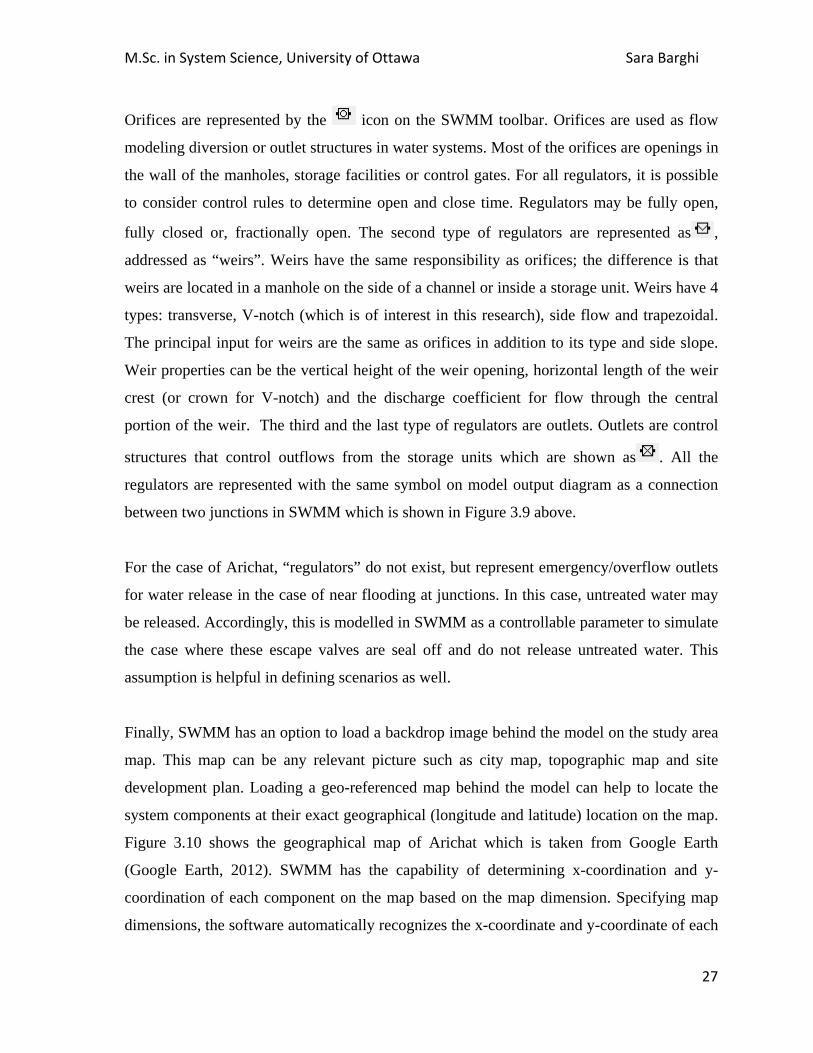
M.Sc. in System Science, University of Ottawa Sara Barghi
27
Orifices are represented by the icon on the SWMM toolbar. Orifices are used as flow
modeling diversion or outlet structures in water systems. Most of the orifices are openings in
the wall of the manholes, storage facilities or control gates. For all regulators, it is possible
to consider control rules to determine open and close time. Regulators may be fully open,
fully closed or, fractionally open. The second type of regulators are represented as ,
addressed as “weirs”. Weirs have the same responsibility as orifices; the difference is that
weirs are located in a manhole on the side of a channel or inside a storage unit. Weirs have 4
types: transverse, V-notch (which is of interest in this research), side flow and trapezoidal.
The principal input for weirs are the same as orifices in addition to its type and side slope.
Weir properties can be the vertical height of the weir opening, horizontal length of the weir
crest (or crown for V-notch) and the discharge coefficient for flow through the central
portion of the weir. The third and the last type of regulators are outlets. Outlets are control
structures that control outflows from the storage units which are shown as . All the
regulators are represented with the same symbol on model output diagram as a connection
between two junctions in SWMM which is shown in Figure 3.9 above.
For the case of Arichat, “regulators” do not exist, but represent emergency/overflow outlets
for water release in the case of near flooding at junctions. In this case, untreated water may
be released. Accordingly, this is modelled in SWMM as a controllable parameter to simulate
the case where these escape valves are seal off and do not release untreated water. This
assumption is helpful in defining scenarios as well.
Finally, SWMM has an option to load a backdrop image behind the model on the study area
map. This map can be any relevant picture such as city map, topographic map and site
development plan. Loading a geo-referenced map behind the model can help to locate the
system components at their exact geographical (longitude and latitude) location on the map.
Figure 3.10 shows the geographical map of Arichat which is taken from Google Earth
(Google Earth, 2012). SWMM has the capability of determining x-coordination and y-
coordination of each component on the map based on the map dimension. Specifying map
dimensions, the software automatically recognizes the x-coordinate and y-coordinate of each

M.Sc. in System Science, University of Ottawa Sara Barghi
28
component on the map. This feature is helpful to find the length of the conduits and area of
the subcatchments (addressed as Auto-length in the software).
Figure 3.10. Isle Madame water system model developed in SWMM
Figure 3.11. Geographical map of Arichat used as the backdrop image of the model Isle Madame water system model in SWMM
(Source: Google Earth, 2012)

M.Sc. in System Science, University of Ottawa Sara Barghi
29
3.3. SWMM Settings and Inputs
In the SWMM simulation option section, general settings, dates and time steps settings are
required to be defined. In the general settings section, it is possible to choose process models
among: (i) different flow routing options, (ii) precipitation, i.e., rainfall/runoff, (iii) tidal
flow routing and (iv) water quality. Choosing any of these options results in a different final
report on SWMM. In the miscellaneous settings section, there are options related to ponding
allowance and report summary options. Infiltration models are other choices in this section.
Infiltration models can be chosen from Horton equation, Green-Ampt method and Curve
Number method. The Horton equation decreases infiltration exponentially from an initial
maximum value to a minimum rate during a huge rainfall. Green-Ampt method assumes a
wetting front in the soil in which an initial moisture soil is separated from saturated soil
above. The third method estimates runoff based on its curve number and total infiltration
capacity.
Date settings in SWMM include start analysis date, start and end reporting dates, start and
end sweeping dates, and the number of anticipated dry days. For time steps in the
simulation, reporting time steps, dry weather runoff, and wet weather runoff time steps are
available options.
(i) Flow Routing Models
Flow routing model is the last option in the “general settings” in SWMM. Flow routing
within a conduit in SWMM is governed by the conservation of mass and momentum
equations for an unsteady flow. These equations are the Saint Venant flow equations. The
flow routing option is used in this simulation and there are three ways to solve these
equations. The first one is steady flow routing which is the simplest method to solve the
equation. When this method is used, it means within each time step flow is uniform and
steady. Therefore, the inflow hydrographs at the upstream end of the conduit flows to the
downstream end without any delay or change in shape. This is the simplest routing method
which cannot be considered for channel storage, backflow effects, entrance losses, exit

M.Sc. in System Science, University of Ottawa Sara Barghi
30
losses, reverse flow and pressurized flow. This method is proper for preliminary analysis
with long-term continuous simulations in SWMM (Rossman, 2010).
The second routing method is kinematic wave routing. This method allows flow and area to
vary both spatially and temporally within a conduit, however this form of routing cannot
account for backwater effects, entrance/exit losses and flow reversal. It can usually maintain
numerical stability with moderately large time steps, therefore it can be used as an accurate
and efficient routing method for long-term simulations (Rossman, 2010) .
The third method is dynamic wave routing. Unlike the other two methods, dynamic wave
routing can be used for channel storage, backwater, entrance/exit losses, flow reversal and
pressurized, which is the case in this research for Arichat.
(ii) Precipitation
The Climatology editor in SWMM is helpful to import time series from climate files. These
time series can be related to precipitation, temperature, evaporation, wind speed, snow melt
and areal depletion.
One of the most important hydrological inputs in SWMM is the precepitation time series.
The Rain gauge is the representative input which is shown with the icon in the SWMM
toolbar and can be added to the study area map in SWMM. Figures 3.10 and 3.11 show
gauge1 which is a rain gauge for the Arichat developed model. Rain gauges, similar to other
physical components, have their specific properties. Rain format is one of these properties
with options for Intensity, Volume and Cumulative Volume. Time interval for precipitation
data and precipitation time series are other principal properties for a rain gauge. It is possible
to define different hourly precipitation time series in SWMM.

M.Sc. in System Science, University of Ottawa Sara Barghi
31
Figure 3.12. Rain gauge representation in SWMM
(iii) Tidal Flow
The Curve section in SWMM defines pump, storage, control, diversion, rating, shape and
tidal curves. The most important curve for the Isle Madamee coastal model is the tidal curve,
which can be defined as hourly time series for tidal levels. Many factors cause tides at any
coastal zone. These factors can be the consequence of the response of the ocean basin to the
tide producing forces, to the variations of tides because of the shallow water effects of local
rivers, or to the regional effects of weather change on water levels. Tides can be high or low.
A high tide is produced by the horizontal flow of water toward the area with maximum solar
and lunar attractions, which results in “heaping” action. On the other hand low tides are
produced by a compensating withdrawal of water. The alternation of these two kinds of tides
is the result of daily rotation of the Earth (International Hydrographic Bureau, 2005).
Highest high tides and lowest low tide effects on the water system in Isle Madame are in
interest of this research. One of the most important effects of tides can be the backflow in
the water system, especially in the treatment plant. The tidal curves for Arichat will be
discussed in scenarios to check the capacity of the system under different tidal levels.
(iv) Water Quality

M.Sc. in System Science, University of Ottawa Sara Barghi
32
SWMM is capable of tracking water quality. Based on this capability, a variety of pollutants
can be defined in SWMM. Defining these pollutants requires defining land uses of the
subcatchments. In each land use definition, water build-up and washoff functions are
determinable. Effluent Build-up functions are described by a mass per unit of the
subcatchment area. The Effluent Build-up, B is a function of the number of dry weather days
and can be described in 3 kind of functions: 1. Power Function, 2. Exponential Function, and
3. Saturation Function. The SWMM functions for B are defined mathematically below.
1.Power Function = ( , )
where = maximum build-up possible (mass per unit of area or curb length) and = build-
up rate constant, and = time exponent.
2.Exponential Function = (1 − )
where = maximum buildup possible (mass per unit of area or curb length) and =buildup
rate constant(1/days).
3.Saturation Function
= +
where = maximum buildup possible(mass per unit area or curb length) and = half-
saturation constant (days to reach half of the maximum).
On the other hand, pollutant washoff may also be defined by one of these functions below:
1.Exponentail Washoff =
where = washoff coefficient, = washoff exponent, q= runoff rate per unit
area(inches/hour or mm/hour), and B= pollutant buildup in mass units.

M.Sc. in System Science, University of Ottawa Sara Barghi
33
2.Rating Curve Washoff =
where = washoff coefficient, = washoff exponent, and Q= runoff rate in user-defined
flow units.
3.Event Mean Concentration (EMC)
This function is a special case of rating curve washoff where is 1.0 and shows the
washoff pollutant concentration in mass per liter. Typical EMC’s for selected pollutants can
be found in Table 3.1. These values show the best values for EMC in a water system. For
each of them there is a maximum and a minimum limitation. These limitations shows the
safe range for the washoff for each pollutant. For example, In Arichat water quality
modeling, TSS is used as one of the pollutants with EMC function as the washoff function.
The washoff coefficient is considered equal to 100. Therefore as it is TSS (Total Suspended
Solid) , based on values in Table 3.1, EMC should be between 180- 584 mg/L.
Finally, in each outfall it is possible to choose if the outfall is connected to a treatment plant
or not. If yes, for each pollutants there should be a treatment expression which has the
general form of one of the two forms below: = ( , _ , ), or = ( , _ , ) where:
R = fractional removal, (units: % concentration)
C = outlet concentration, (units:mg/L)
P = one or more pollutant names,
R_P = one or more pollutant removals (prepend R_ to pollutant name),
V= one or more process variables (e.g., FLOW(in user-defined flow units), DEPTH(units: m), HRT(hydraulic residence time (units: hours), DT(routing time step (units: sec)), AREA( units: m ).
Table 3.1. Typical EMC’s for selected pollutants

M.Sc. in System Science, University of Ottawa Sara Barghi
34
(Source: Rossman, 2010)
Constituent Event Mean
Concentration
TSS(mg/L) 180-584
BOD(mg/L) 12-19
COD(mg/L) 82-178
Total P(mg/L) 0.42-0.88
Soluble P(mg/L) 0.15-0.28
TKN(mg/L) 1.9-4.18
NO2/NO3-N(mg/L) 0.86-2.2
Total Cu(µg/L) 43-118
Total Pb(µg/L) 182-443
Total Zn(µg/L) 202-633
Based on the inputs and the properties of the SWMM Physical components, a variety of
scenarios can be defined to run the simulation of the water system. In order to define the
simulation scenarios for analysis, the first step is to determine the controllable and
uncontrollable variables of the system as those variables that are important for the purpose
of the community water system policy analysis and research. For example, whether Valves
are open or closed can be considered as controllable variables for the scenarios in this
research. Other variables such as precipitation time series, tidal level, initial depth of the
junctions, and impervious percentage applied to the subcatchment areas are uncontrollable
system variables. The precipitation time series can introduce heavy, mean and light storms
based on the hourly values provided in the series. Tidal level time series can be helpful in
defining highest high tide, lowest low tide and mean tide level in the whole data available
for the tidal levels. Another option for tides can be starting the simulation at low tide or
starting at high tide. All these alternatives make a difference in the scenarios and the
simulation. Initial depth of the junctions can be considered equal to 0, which shows there is
no water present in the junction at the time the simulation starts. Also it can be considered
equal to the maximum depth of the junction at the time the simulation starts. Subcatchment

M.Sc. in System Science, University of Ottawa Sara Barghi
35
impervious percentages can be low or high in different scenarios. Low percentage shows
more infiltration in the subcatchments which results in less inflow into the water system and
high percentage causes less infiltration and more runoff on the subcatchments. Considering
these controllable and uncontrolable variables, scenarios can be defined with the
combination of different alternatives for the SWMM model parameters defined above.
3.4. Outputs in SWMM
Once the model data sets and properties for all components have been defined, the
simulation of the water system performance on SWMM can be carried out. Simulation
results are presented in a variety of SWMM reports. The moment the simulation is
completed, a small window appears on the screen which shows the mass continuty errors for
surface runoff, flow routing and quality routing. These errors show the difference between
initial storage plus total inflow and final storage plus total outflow for the whole water
system. These errors are provided in percentage terms and should not exceed 10%,
otherwise the simulation and data should be checked for possible problems. The most
common reasons for a continuity error more than 10% can be long time steps, or too short
conduits. In addition, the in-status report (explained in the following paragraph) lists the
junctions of the system that have excessive continuity errors. If junctions have continuity
errors greater than %10 then it signals that a review of the junctions should be conducted in
order to reduce the continuity errors is necessary.
SWMM reports results in different formats such as system status reports (e.g., re flooding of
junctions), graphic reports (e.g., on flow rates), table reports (e.g., of junction depth levels)
and statistical reports (e.g., of time in state). A status report includes analysis options, input
summary, rain fall summary, error messages, control actions, continuity errors, stability
results and also summary results for each physical component in the system. Moreover, in
the status report flooding junctions and surcharged conduits and junctions are specified.
Results can be analyzed based on different kinds of graphs in SWMM including time series
plots (e.g., of preciptiation events over the simulated period), scatter plots (e.g., catchment
runoff over nodes total inflow), and profile plots (e.g., tracking water flow in the lower road
conduits).

M.Sc. in System Science, University of Ottawa Sara Barghi
36
Time series graphs depict the value of a particular variable (e.g., flow rates, water depth)
versus the elapsed time. These values are chosen based on the object category (junctions,
conduits, subcathments, total system). Values may include inflow, outflow, depth, and
flooding for each object chosen from the study area map. Also if data, which are pre-defined
data based on some limitations and constraints, be defined for any of the objects, SWMM
has the ability to compare the computed values with the pre-defined data in a graph.
Additionally, the table report displays all data related to graphs.
Scatter plots represent the association between a pair of variables, such as precipitation in a
subcatchment and flow rate in a conduit. Scatter plots are helpful in identifying unstable
flow routing results which SWMM is not capable of doing automatically. Unstable flow
routing occurs when significant fluctuations takes place at certain periods of time in some
junctions. For the Arichat model, status report, time series plots, profile plots and table
reports will be used for analyzing the results.
Profile plots display water flow in conduits and junctions. In this type of plot, it is possible
to track water flows in the system in an animated view. This plot shows what exactly
happens to the junctions and conduits during a simulation.
Lastly, statistical reports can be created from the simulation results time series. This report
separates the simulation period into non-overlapping segments such as; day, month, or by
volume above some minimum threshold values. Then it computes a statistical value for each
event such as mean, maximum or total sum of a variable in the event’s time period. Finally,
it shows a summary of these statistics values for the entire values in all the events. Mostly,
statistical analyses in SWMM are proper for long-term continous simulation runs.
3.5. Process of Research
In this section, the process of the research, SWMM model development and analysis for the
Arichat water system is explained. This section describes how the process is applied.
SWMM is used in this research to model and simulate the water system in Arichat, Isle
Madamee. The stormwater system in Arichat is characterized as a natural system which

M.Sc. in System Science, University of Ottawa Sara Barghi
37
associates with the sewage system through runoffs from catchments to the manholes in the
system. The Arichat sewage system contains 5 pumping stations, one treatment plant, and 95
manholes (Municipality of the County of Richmond, 2003) from which only eleven
manholes will be represented in the model developed in this research. In the Arichat SWMM
model, some of these manholes are connected to subcatchment areas which connect the
natural stormwater system and the sewage system in Arichat.
SWMM is used to develop rundimentary models of the Arichat water system with physical
components (junctions, conduits, subcatchments, storage units, pumps, outfalls and gauges)
and directional flow. Also, a geo-referenced map of Arichat harbour is provided for the
backdrop map in the model and the area of the water system is defined on this map. After
that, geo-referenced and elevation data on water stations and manhole sites are collected
and linked to mapping system in SWMM (the elevations are the result of comparing
handheld GPS elevation values and the RTK(Tienaah et al., 2011) report elevation values).
Technical data and properties on pumping stations is collected from the Municipal Public
Works for each station in Arichat. On the other hand, for the water qulity aspect, an example
from SWMM manual for water quality information for the system is used (in the absence of
actual obsevations). For the inputs of SWMM, historical data on precipitation (Environment
Canada) and on tidal patterns is gathered. Then, events of interest, storms, surge, hurricanes
etc. are analysed. The next step is to define scenarios. For this purpose, the controllable and
uncontrollable parameters of the water system are validated and verified with the
Municipality. In addition to defining variables, a 24-hour simulation model of storm events
based on tidal level information and precipitation time series is prepared. The 24-Hourtimeperiodforthedeterministicsimulationischosenbasedonanacceptedpractice(basedon feedback fromNSgovernmentworkshoponFebruary2013),the duration of severe
storms, and the expected peak capacity impacts on the water system. This time period
enables the analyses of the extreme event and its impacts on the water system. Based on the defined controllable and uncontrollable variables, simulation model scenarios
and output results for analysis are designed. After running the simulation model under each
scenario results and outputs are analyzed. Model results are explicitly examined for system

M.Sc. in System Science, University of Ottawa Sara Barghi
38
policy considerations (i.e., observed water system “weak spots”, implications of severe
storm event impacts, implications of strategic policy changes (e.g., closing outfall regulator
valves, etc.) ). The simulation model water system recommendations are reported and finally
a review of future modelling updates, and monitoring and observations is provided.
In Chapter 4 the detailed research process and the results of the simulation are discussed.
Chapter 5 presents the analysis of the results and outputs.
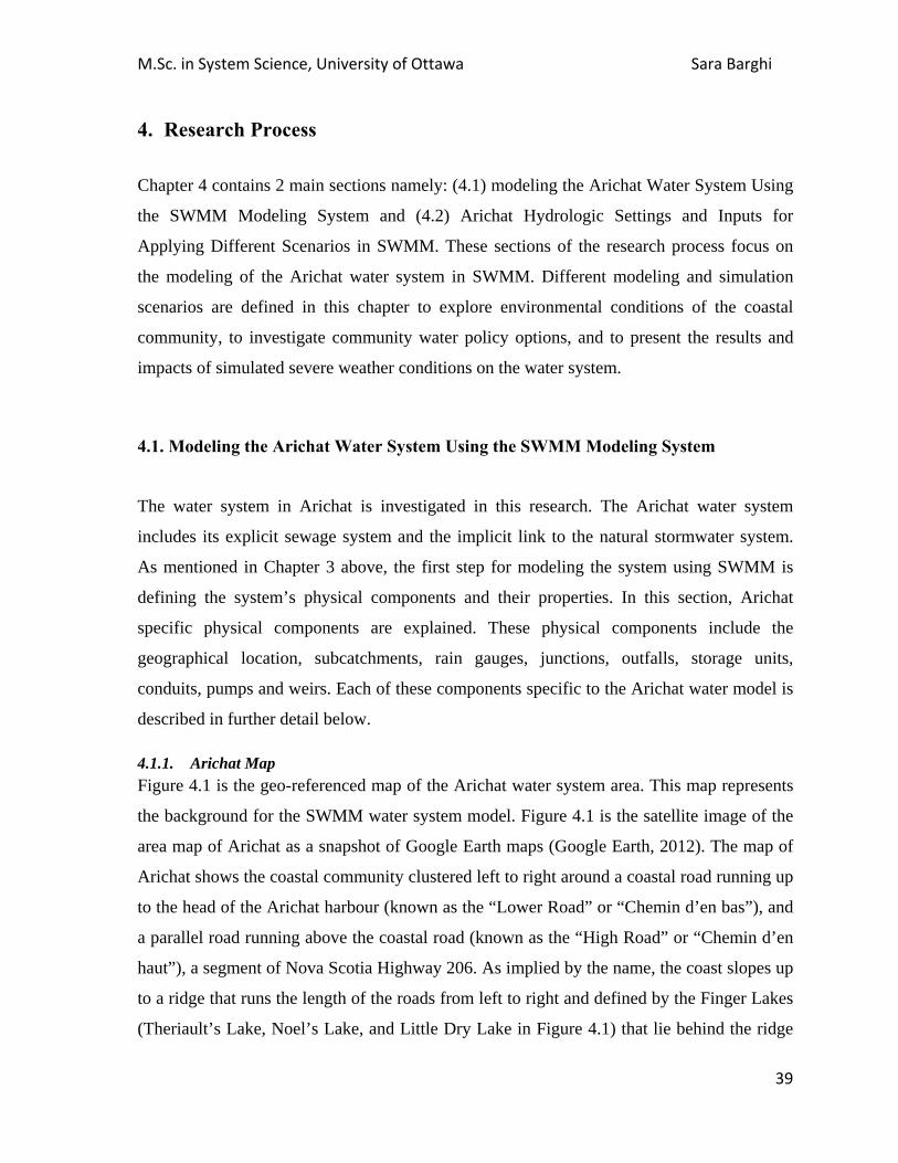
M.Sc. in System Science, University of Ottawa Sara Barghi
39
4. Research Process
Chapter 4 contains 2 main sections namely: (4.1) modeling the Arichat Water System Using
the SWMM Modeling System and (4.2) Arichat Hydrologic Settings and Inputs for
Applying Different Scenarios in SWMM. These sections of the research process focus on
the modeling of the Arichat water system in SWMM. Different modeling and simulation
scenarios are defined in this chapter to explore environmental conditions of the coastal
community, to investigate community water policy options, and to present the results and
impacts of simulated severe weather conditions on the water system.
4.1. Modeling the Arichat Water System Using the SWMM Modeling System
The water system in Arichat is investigated in this research. The Arichat water system
includes its explicit sewage system and the implicit link to the natural stormwater system.
As mentioned in Chapter 3 above, the first step for modeling the system using SWMM is
defining the system’s physical components and their properties. In this section, Arichat
specific physical components are explained. These physical components include the
geographical location, subcatchments, rain gauges, junctions, outfalls, storage units,
conduits, pumps and weirs. Each of these components specific to the Arichat water model is
described in further detail below.
4.1.1. Arichat Map Figure 4.1 is the geo-referenced map of the Arichat water system area. This map represents
the background for the SWMM water system model. Figure 4.1 is the satellite image of the
area map of Arichat as a snapshot of Google Earth maps (Google Earth, 2012). The map of
Arichat shows the coastal community clustered left to right around a coastal road running up
to the head of the Arichat harbour (known as the “Lower Road” or “Chemin d’en bas”), and
a parallel road running above the coastal road (known as the “High Road” or “Chemin d’en
haut”), a segment of Nova Scotia Highway 206. As implied by the name, the coast slopes up
to a ridge that runs the length of the roads from left to right and defined by the Finger Lakes
(Theriault’s Lake, Noel’s Lake, and Little Dry Lake in Figure 4.1) that lie behind the ridge

M.Sc. in System Science, University of Ottawa Sara Barghi
40
and oriented in the same direction as the roadways. Community dwellings lie along the
length of the roads on the shore side of the Lower (coastal) Road, and either side of the High
Road evident from the map of Figure 4.1.
Figure 4.1. Arichat model's backdrop image (Arichat map)
Source: (Google Earth, 2012)
4.1.2. Model Subcatchments The water system in Arichat, Isle Madame is developed in SWMM by applying the junction-
links model to the pipe system there. The developed model is shown in Figure 4.2. The area
is divided into 13 subcatchments from “S1” to “S13”. As noted in Figure 4.2, subcatchments
S1 to S6 lie between the High Road and the high point of the ridge overlooking the Finger
Lakes. These subcatchments over the High Road are located in a residential area of relative
low density of houses and buildings. Subcatchments S7 to S13 are defined in the space
between the High Road and the Lower Road. These 7 subcatchments are located between
the higher and the lower roads and are more developed areas with residential and
commercial usages.

M.Sc
Figu
Subc
alon
Sinc
same
gaug
Thes
c. in System
ure 4.2. Aric
catchment p
g the High
ce the area u
e in the diffe
ge is applied
se precipitati
Science, Un
chat water sy
properties ar
Road. Each
under investi
ferent subcat
d to the who
ion data are
Table
Prope
Name
Rain Gauge
Outlet
Area
Impervious
Land uses
iversity of O
ystem model
re shown in
h of the sub
igation is rel
tchments of
ole area for
defined as ti
e 4.1. Sampl
erty
S
e G
j
2
s (%) 2
2
Ottawa
l in SWMM
Table 4.1 b
bcatchments
latively sma
the whole m
injection of
ime series in
le subcatchm
S3
Gauge1
3
23.89 ha
25 %
2 (High Road
M with subcat
below for th
s receives p
all, the precip
model. There
f precipitatio
n SWMM.
ment propert
Value
d area, “less
tchments S1
he case of s
recipitation
pitation is a
efore, in this
on data to th
ties:S3
s developed”
Sara Barg
to S13 indic
subcatchmen
from “Gau
assumed to b
s model only
he water sy
”)
ghi
41
cated
nt S3
uge1”.
be the
y one
ystem.

M.Sc. in System Science, University of Ottawa Sara Barghi
42
In the subcatchment property table of Table 4.1, junction “j3” is considered as the “Outlet”
for subcatchment S3 which receives the catchment runoff. In the Arichat model,
subcatchments S1 through S13 are connected to the junctions: j1, j2, j3, j4, j5, j16, j6, j8,
j10, TreatmentPlant, j13, j13 and j15, respectively.
4.1.3. Arichat Map Geo-referencing SWMM has an auto-length option, which determines the length of the pipes (“conduit”) and
area of subcatchments automatically when real geo-referenced coordinate values are
provided in the model data. In this regard, the upper-right and lower-left X-coordinate and
Y-coordinate are defined in the “dimensions” window in SWMM. In order to find these
values, the map scale is used to find the length of each pixel of the background image used
for this model. This scale can be found on the left bottom of the backdrop image in Figures
4.1 and 4.2 above. The length of the scale line on the map is 2680 feet (or 817 m) as noted
on the image scale. Using the Photoshop software (Photoshop, 2013) the number of pixels of
this line is determined as 291 pixels. Therefore based on the ratio calculation 2680 feet/291
pixels, each pixel in this image is 9.21feet/pixel (2.8 meters/pixel).
Now by finding the number of pixels on the length and width of the image it is possible to
find the real values for these lengths. Photoshop was used to determine the pixel values for
the background image. The length of the image is 1440 pixels and the width is 817 pixels.
As noted above, each pixel is 2.8 meters. Therefore, the length of the map image (Figure 4.1
and 4.2) is determined as 1440 pixels in length or 1440 pixels times 2.8 meters/pixel or 4032
meters. Similarly, the width of the map image is determined as 817 pixels in length or 817
pixels times 2.8 meters/pixel or 2287.6 meters.
The lower-left X-coordinate and Y-coordinate are considered as the map origin or point
(0, 0). Based on this assumption, the upper-right X-coordinate and Y-coordinate is point
(4032, 2287.6). With these values, the auto-length option in the software is turned “on”, and
the real length of the pipes and real area for subcatchments are determined automatically
from the map grid.

M.Sc. in System Science, University of Ottawa Sara Barghi
43
4.1.4. Subcatchment Impervious Characteristics As noted in Chapter 3, subcatchments are characterized by their pervious and impervious
natures. In general, the impervious percentage (impenetrable proportion of land with respect
to water run-off) for the upper model subcatchments (i.e., subcatchments S1 through S6
above the High Road) that are comprised mainly of fields and undeveloped terrain, is set at
25% representing the estimate of precipitation that can be considered to flow off the soil and
into the sewage (through manholes) or the natural stormwater system (in culverts and
drains). The higher subcatchments are located in more undeveloped area and this causes
more ground infiltration and respectively a lower impervious percentage. The impervious
value is higher (estimated at 50%) for the lower coastal subcatchments (S7 through S13)
along the Lower Road because these subcatchments are more residential and contain paved
or graveled driveways, parking lots and asphalt roads.
4.1.5. Water Quality and Common Pollutants Before assigning land uses to the subcatchments, each subcatchment needs to be defined in
terms of water quality and pollutants present. Unfortunately, there are insufficient data
available regarding the status of water quality and the presence of pollutants in Arichat. To
compensate for these data deficiencies, data applied to the Arichat model is taken from
standard water system water quality examples provided in the SWMM manual (Rossman,
2010). In this example, two types of common water borne pollutants are introduced, TSS
(Total Suspended Solids) and Lead, a co-pollutant of TSS. The co-fraction of TSS for Lead
is considered as 0.25 in this model applied as an estimate (as stated in the SWMM manual
example).
4.1.6. Land Use Buildup and wash-off of pollutants from each subcatchment are assigned through the land
uses option on the subcatchment properties table. Two types of land uses are defined in this
model: residential and undeveloped. For residential land use, the exponential function is
chosen as the build-up function for TSS with maximum build up equal to 75 kg per unit of
normalizer with the normalizer being the area of the subcatchment, e.g., as noted in Table
4.1 for S3. Normalizer is the variable to which TSS build up is normalized on a per unit
basis. The constant rate is 1 for this equation. The Wash-off function for TSS in residential
land use is an Event Mean Concentration (EMC) function with 100 as its coefficient. For

M.Sc. in System Science, University of Ottawa Sara Barghi
44
undeveloped subcatchments areas, there is no function defined for build-up and wash-off
function as no such pollutants (e.g., TSS) are produced in these kinds of areas. As mentioned
before, the subcatchments on the High Road are primarily undeveloped terrain and the
subcatchments in between the upper and the lower road are mostly residential. Taking this
into account, land uses percentages can be defined for each subcatchment. Residential
percentages will be stated here. Subcatchments S1 through S13 have their residential
percentages equal to 10%, 40%, 25%, 25%, 30%, 30%, 30%,75%, 75%, 80%, 80%, 75%
and 75%, respectively.
4.1.7. Model Junctions and Storage Units Arichat has 95 manholes (Municipality of the County of Richmond, 2003). Twelve of these
manholes are used for the description of the Arichat water system. These 12 manholes are
shown as junctions j1 to j12 in this model (Figure 4.2). Five other junctions are represented
as storage units that are used to represent inlet of pumps to the model. In this model, the
pipeline along the High Road of Figure 4.2 is defined as being on a rise with specific
elevations and slopes relative to the coastal area. As such, the modeled system, like the
actual case for Arichat, uses gravity and water which comes from catchments at higher areas
to go through connections (“j1” through “j16”) between upper (higher) and lower (near
coast) pipes. At the end of the water system, sewage water exits the system through the
outlet (“TreatmentPlantOutfall (TPO)”) corresponding to the town’s treatment plant in
Arichat harbor at the junction near LeNoir Forge (Figure 4.2).
Junctions and storage units are the most important components in this model. The most
significant property of a junction and a storage unit is its elevation. For the High Road
junctions’ elevation, two sets of data are investigated in this regard. The first set is taken
from (Tiennah et al., 2011) where a Real Time Kinematic (RTK) GPS survey was
undertaken on Isle Madame, Nova Scotia. The second set is observations from a hand held
GPS. Both datasets are used to establish elevations for different points in Arichat. In both of
the sets, selected coordinates are specified for each point. The two sets of data are compared.
Common points were found in order to compare and contrast the different elevation
estimates. Four points were found in common based on the longitudes and latitudes, as
shown in Table 4.2. The Treatment Plant is set as the benchmark of the system with the

M.Sc. in System Science, University of Ottawa Sara Barghi
45
elevation of the Treatment Plant considered as 0, or the same as the sea level. Other point
elevations are considered as relative elevations to the Treatment Plant benchmark elevation
level. It is considered, despite their predicted higher accuracy that the relative elevation for
the limited RTK point values recorded in (Tiennah et al., 2011) (Table 4.3) appear to be
different from expectations. Therefore, given the more complete set of the hand held GPS
data set, these values (Table 4.2) are chosen as the applicable data for higher road junctions’
elevations. In the Arichat SWMM simulation model, the relative elevations of Table 4.2
were used as the main data in the model.
The Municipality of County of Richmond in which Arichat is located have provided
documents regarding the Arichat pumping stations site location plan, as well as the Arichat
pumping station electrical plans sections and details (CBCL Limited,2010). For the Lower
Road invert elevations, the technical data available in these documents are used to define the
junctions’ characteristics. Invert elevation, maximum depth and surcharge depth for
junctions and storage units are all available in these documents. Table 4.4 presents the
junction’s properties for junction j11 (Figure 4.2). Table 4.5 presents the storage unit
properties for junction j10 (Figure 4.2).
On the Lower Road, 5 pumping stations exist. Each pumping station has an inlet and an
outlet. Outlets are represented by junctions and inlets are represented by storage units. In the
documents provided by the Municipality, inlets are introduced as wet wells. In sewage
systems which contain pumping stations, wet wells are used to store sewage and then when
the level of sewage increases to a specific level in the wet well, the pump will start working
and will pump up the sewage, stopping when a specific low level is achieved. In SWMM,
wet wells can be shown as storage units. Therefore, it is obvious that the elevation of each
junction should be higher than the elevation of each storage unit in a pumping station so the
pump can lift the water from the lower elevation to the higher elevation.
The only junction, who has an extra property, is the “TreatmentPlant” junction. In order to
simulate Arichat’s treatment plant capacity, a “ponded area” is used for this junction. The
ponded area for this junction is considered equal to 100 and for other junctions this area

M.Sc. in System Science, University of Ottawa Sara Barghi
46
is 0. The initial depth of each junction is considered as a controllable variable for scenarios
which can be either 0 or equal to the maximum depth.
Table 4.2.Hand held GPS data used for the simulation
Points Description GPS Long-Lat
GPS Elevations(m)
Relative GPS Elevations(m)
1 Near Dede and Thomas Boudreau’s house
45 30.486 -61 02.308 9.144 2.74
2 Michel Samson’s house 45 30.576 61 01.700 7.31 0.91
3 Funeral Home 45 30.656 61 01.013 6.4 0
4 Sewer system-Lenoir forge(benchmark)
45 30.649 61 00.752 6.4 0
5 Herman Samson’s house 45 30.730 61 00.179 7.31 0.91
6 Before the two wharves 45 30.766 60.59.516 6.7 0.3
7 Corner of intersection with the church
45 30.615 61 01.976 28.96 22.56
8 Jeanties mini mart 45 30.649 61 01.723 24.08 17.68
9 Dan Mac Hardware store 45 30.648 61 01.616 20.73 14.33
10 Pharmacy 45 30.652 61 01.526 21.94 15.54
11 Old liquor store 45 30.658 61 01.436 24.69 18.29
12 Shirley’s spud wagon 45 30.692 61 01. 288 22.86 16.46
13 Anglican church 45 30.704 61 01.116 23.47 17.07
14 Post office 45 30.722 61 00.971 22.55 16.15
15 Court house 45 30.725 61 00.886 21.94 15.54
16 Sporty’s 45 30.740 61 0.616 26.51 20.11

M.Sc. in System Science, University of Ottawa Sara Barghi
47
Table 4.3. RTK survey and hand held GPS elevations and their relative elevations
Table 4.4. Model Sample junction properties: j11
Properties Value
Name j11
Invert elevation (m) 1.64
Maximum depth (m) 4.274
Initial depth (m) 0
Surcharge depth (m) 1.683
Ponded area (m2) 0
Table 4.5. Sample storage unit properties: j10
Properties Value
Name j10
Invert elevation (m) -0.92
Maximum depth (m) 4.347
Points Description RTK long-lat GPS Long-Lat
RTK Elevations(m)
GPS Elevations
(m)
RTK Relative
Elevations(m)
Hand Held
GPS Relative Elevations(m)
1
Near Dede and Thomas
Boudreau’s house
45 30 29.16 -61 02 18.58
45 30.486 -61 02.308 -9.0 9.144 3.52 2.74
2 Michel
Samson’s house
45 30 34.21 61 1 41.27
45 30.576 61 01.700 -10.763 7.31 1.76 0.91
3 Funeral Home
45 30 39.29 61 1 0.70
And 45 30 39.31
61 1 0.83
45 30.656 61 01.013
-10.9 (average of two close
points)
6.4 1.62 0
4 Sewer system-Lenoir forge
45 30 36.70 61 0 42.67
45 30.649 61 00.752 -12.521 6.4 0 0

M.Sc. in System Science, University of Ottawa Sara Barghi
48
4.1.8. Model Conduits Other important components of the Arichat model are conduits (pipes) which are the
connections between the junctions. The three available properties for pipes are: (i) pipes
diameter which is shown as the maximum depth of the pipe in the software; (ii) the length of
pipes; and (iii) the shape of each pipe. For pipes along the High Road (“c1” to “c4”), the
Lower Road (“c10” to “c14” and “c15”) and the pipes connecting lower and higher road
pipes, the diameter of the pipes is 0.1524 meters (6 inches), 0.2560 meters (10 inches) and
0.7112 meters (28 inches), respectively (Boudreau, 2013). The connecting pipes which
connect high to low road pipes are considered as culverts, that is why their diameter is
considered larger than normal. The length of each pipe is defined according to the auto-
length option in SWMM. Shape of the all the pipes is circular (Boudreau, 2013). Table 4.6
shows conduit c7 properties as an example.
Table 4.6. Sample conduit properties: c7
4.1.9. Pumps In the water system in Arichat there are 5 pumping stations. As explained in section 4.1.7,
the pumping stations each have a junction as the outlet and a storage unit as the inlet point of
the station. Similar to all other components, pumps have different properties. In the
documents provided by the Municipality of the Richmond County, the technical properties
of the specific pumps are available. Based on the specific codes provided for each pump in
these documents, it is possible to find pump performance curves. The manufacturing
company of the pumps has provided these curves on its website (Xylect Professional, 2013).
Property Value
Name c7
Inlet junction J3
Outlet junction J10
Shape circular
Max. depth 0.7112 meters
length 156.41
Flap gate No

M.Sc. in System Science, University of Ottawa Sara Barghi
49
Properties of a sample pump, p3, are shown in Table 4.7. Pump p3 performance curve is
also shown in Figure 4.3.
Table 4.7. Sample pumps properties: p3
Property Value
Name P3
Inlet junction j10
Outlet junction j11
Pump curve P3
Initial status ON
Startup depth (m) 1.524
Shutoff depth (m) 1.067
Figure 4.3. A sample pump, p3, performance curve
In Figures 4.4 and 4.5, images of pump stations are shown to give an actual view of the area.
The location of each manhole and each pumping station is defined with the help of the
longitude and latitude from the handheld GPS. These coordinate values are found in Table
4.2 above. These values are then matched with the background image in this model. The
pictures shown in Figure 4.4 and 4.5 are of the 5 pumping stations in Arichat in addition to
pictures of the treatment plant facilities in Arichat. As noted in the illustrations, these

M.Sc. in System Science, University of Ottawa Sara Barghi
50
stations are recently installed new stations for the delivery of Arichat sewage water to the
Treatment Plant near LeNoir forge.
4.1.10. Regulators In coastal zones, storm surge affects the stormwater system. As the storm generates
increased precipitation, there will be potential stormwater backups in the system if flow
capacity is exceeded with the result being flooded junctions and possibly flooded basements.
In order to prevent and control these backups, 6 regulators and 6 outfalls (to Arichat
Harbour directly) are included in the modeled Arichat water system. Therefore, whenever
junctions j6, j8, j10, j13, j15 and the treatment plant reach flood status from the incursion of
stormwater, the regulators help prevent backups as they have gates that are triggered to open
automatically to the outfall when the local pipes and junctions reach a pre-specified level of
capacity. These regulators and controls apparently do not exist in the actual system currently
in place in the Arichat water system. These controls are added to the model in order to
model their existence as potentially helpful to prevent backups and flooding. Another reason
to use these regulators is that in SWMM, it is not possible to show the connection of several
conduits to a junction. On the other hand, the documents provided by Municipality of
Richmond County for pumping station’s plan (CBCL Limited, 2010) shows an extra
connection to the storage units, an overflow which directs water into the Arichat harbour at a
specific height of water in the storage unit. In order to show this connection, regulators are
helpful representations. The height of the regulator can be considered as the specific height
provided in the pumping station plan and the length of the regulator can be considered as the
diameter of the connection. Based on these plans, the height for each regulator is 2.591
meters and the remaining height above this height will be considered as the surcharge depth
for the outlet junction of the pumping station (refer also to section 4.1.3). The length of each
regulator is equal to 10 inches (0.254 m) based on the real observations. Based on the
technical data provided (Municipality of Richmond County, 2007), all the regulators
existing in the real system are considered in SWMM as “weirs” of type “V-NOTCH”, as
consistent with the technical data provided. Therefore, all the added regulators are
considered similar to other regulators in the system. As mentioned in Chapter 3, V-NOTCH
regulators have a standard discharge coefficient equal to 1.35 CMS. Table 4.8 shows R3
properties as a sample regulator.
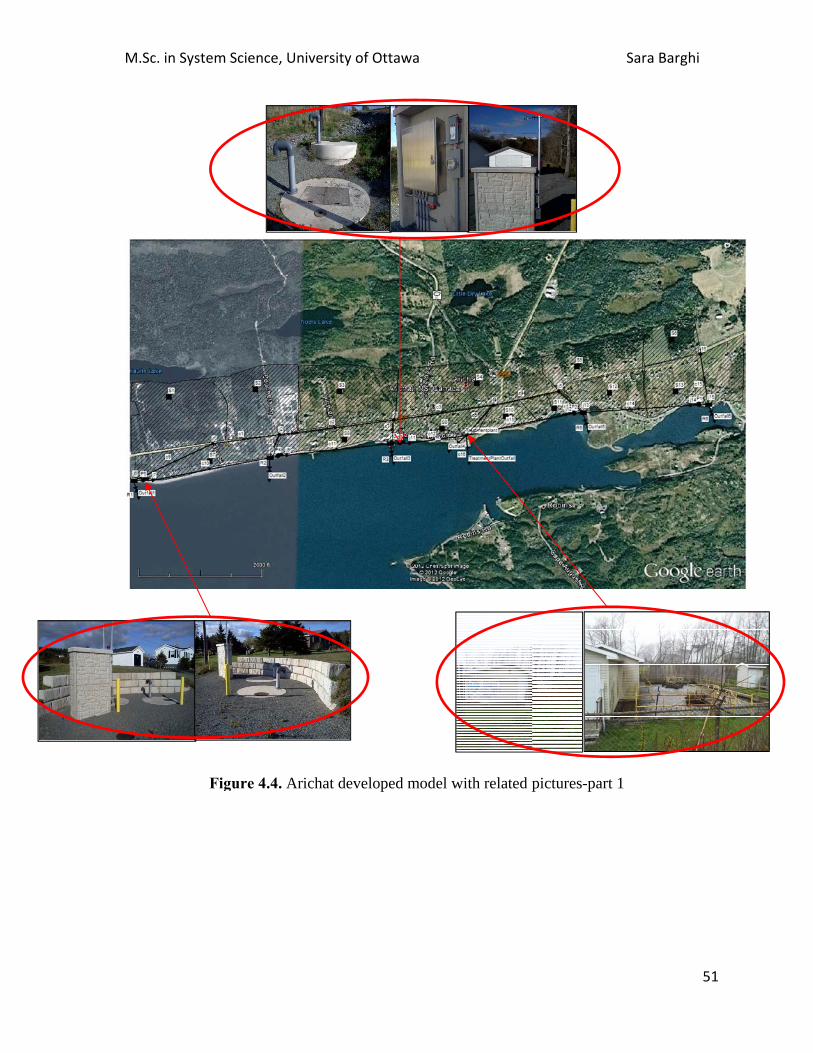
M.Sc
c. in System
Fig
Science, Un
gure 4.4. Ari
iversity of O
ichat develo
Ottawa
ped model w
with related p
pictures-part
Sara Barg
t 1
ghi
51

M.Sc
c. in System
Fi
Science, Un
igure 4.5. A
iversity of O
Arichat devel
Ottawa
oped model
with related
d pictures-pa
Sara Barg
art 2
ghi
52

M.Sc. in System Science, University of Ottawa Sara Barghi
53
Table 4.8. Sample regulators properties: R3
Properties Value Name R3 Inlet junction j10 Outlet junction Outfall3 Type V-NOTCH Height (m) 2.591 Length (m) 0.254 Discharge Coefficient(CMS) 1.35
It is also possible to define control rules for pumps and regulators in SWMM. Rules can be
defined in a way to let the valves be open permanently, be closed temporarily or
permanently and also they can be half-open in some specific situations or permanently be
half open. These control rules are helpful to define the scenarios and are discussed in further
detail below (section 4.2.1 below).
4.1.11. Outfalls Outfalls are components in the Arichat water system that are the connection between the
system and the open water of the Arichat harbour. The treated or untreated water flows into
the harbour through these outfalls. The outfall connected to the Treatment Plant is the main
outfall in this model. When there is no storm or any unusual precipitation in the system, the
system would work normally which means the runoff from the subcatchments flows into the
system, and the water will flow to the “TreatmentPlant” junction, the location of the
Treatment Plant. The water is treated at the plant and then the treated water will flow to the
“TreatmentPlantOutfall”.
There are six other outfalls which are connected to the regulators. In case of overload in any
of the storage units in the system, untreated water will flow into the harbour through these
outfalls based on the control rules applied on the related regulators. Since these outfalls are
the connections to the harbour, they directly sense the ocean tidal levels. Therefore, in the
property table for outfalls there is a choice to choose tidal outfalls. The type of the outfalls
other than “TreatmentPlant Outfall” is chosen as “tidal” and can be defined by a curve. The
curve shows the relation between the sea level and the time of the day. Initial tidal data were
applied hourly tide levels provided by Fisheries and Oceans Canada for North Sydney

M.Sc. in System Science, University of Ottawa Sara Barghi
54
located in Nova Scotia and used as proxy tides for Arichat habour. Table 4.9 shows Outfall1
properties as an example. Since the treatment plant is usually the most downstream end of
the collection system, it is represented as an outfall junction with a “fixed head” (Rossman,
2013). Therefore, “TreatmentPlantOutfall” type is a fixed head outfall with fixed stage equal
to 0 instead of being an outfall with a curve. Moreover, as it is the outfall connected to the
Treatment Plant, it should have the treatment option in its properties as mentioned
previously in Chapter 3. In order to turn on the treatment option, the following treatment
plant expression is used for TSS pollutant in this outfall: = 0.523 × . × .
This equation is an example used in the SWMM model for water quality investigations
(Rossman, 2010). This example is used because there are not enough data available for the
treatment plant in Arichat. The invert elevation for each outfall is considered to be equal to
the invert elevation of each storage unit, so it will be lower than the height of the regulator
where water flows into the outfall. When the water level in the outfall gets to this height in
the connected storage unit, it flows out into the harbor.
Table 4.9. Sample outfall properties: Outfall3
Properties Value
Name Outfall3
Inflows NO
Treatment NO
Invert elevation (m) -0.92
Tide gate NO
Type Tidal
Curve name Depending on the Scenario a Tidal Time Series
is used as the tidal curve for an Outfall

M.Sc. in System Science, University of Ottawa Sara Barghi
55
4.2. Arichat Hydrologic Settings and Inputs for Applying Different Scenarios in SWMM
After modeling the Arichat stormwater system, different storm scenarios may be applied to
the system. These scenarios can be defined by different precipitation intensity, different time
series for rainfall gauges, different tide levels, and different properties for each component
in the system. Uncontrollable and controllable variables can be defined in all these
scenarios. In this section controllable and uncontrollable variables are introduced with their
different alternatives to define the simulation scenarios.
In these simulations, control rules for regulators are considered as the controllable variables.
Uncontrollable variables are introduced as precipitation intensity, tidal level, initial depth of
the junctions, and impervious percentage for higher and lower subcatchments. For each of
these variables different parameter values are provided to define the scenarios.
4.2.1. Controllable variables: Regulators As mentioned above, regulators are considered as controllable variables. There are 6
regulators that can have 2 alternatives status settings: closed or open. In this research, all
regulators are considered to have the same situation at all times, i.e., the 6 regulators are
open or closed simultaneously. It means all the regulators obey the same control rule which
makes them open or close. For each regulator, the depth of the storage unit is used as the
factor that triggers opening closed regulators. This depth is equal to the height of the
regulator. If water gets to this depth in the storage unit or more, then the regulator will open
and water will flow directly to the harbour through the connected outfall. Resetting the weir
of the regulator equal to 1 changes the regulator status from closed (=0) to open (=1). The
control rules defined for opening regulators are the same for all regulators. j6, j8, j10,
TreatmentPlant, j13, and j15 move from the initial status of closed to open when the depth
of the node is greater than or equal to 2.591m. The SWMM code for these control variables
are provided in Appendix B– SWWM Model Reglatures Rules Definition.
The control rules for defining “closed” alternative for regulators is the same as above, but
instead of 1 in front of the second line of each rule one should consider 0, which is provided
in Appendix B. It means that the regulators are closed at all the times.

M.Sc. in System Science, University of Ottawa Sara Barghi
56
4.2.2. Uncontrollable variables
4.2.2.1. Precipitation Uncontrollable variables play important roles in the simulation of this system. The
precipitation data for running the Arichat water model are the precipitation time series
provided by Environment Canada, Atlantic operations for Tracadie, Nova Scotia. Tracadie is
used as a “proxy” for Arichat given that these data, presented in an Excel file, are the closest
location to Arichat among the available data. The data are hourly data which start at 2:00pm
on the 14th of April, 2004, and end at 4:00am on the 22nd of October 2011. The average
monthly precipitations for these 7 years from these data are shown in Table 4.10 below.
Table 4.10. Monthly average precipitation for the seven-year data set, 2004 to 2011
Source: (Environment Canada, 2012).
Number Month
Average hourly
Precipitation
(mm)
1 January 0.13181338
2 February 0.099889
3 March 1.6
4 April 0.102839
5 May 0.09995
6 June 0.118096
7 July 0.116167
8 August 0.140054
9 September 0.103023
10 October 0.174237
11 November 0.159434
12 December 0.187238

M.Sc. in System Science, University of Ottawa Sara Barghi
57
Over the 7 year period, the maximum precipitation took place in March during these 7 years
and the minimum precipitation took place in the month of February. The related histograms
(Figure A1 and Figure A2) in these two months are found in Appendix A – Precipitation
Data Summary.
In SWMM, a 24-hour time series is defined to introduce each precipitation alternative. Four
alternatives are considered in the simulation model for applying the precipitation data. The
first alternative is “Off” which shows a minimum precipitation in a 24-hour simulation in
the system. The minimum hourly value for the precipitation in the seven years data is
0.3mm/hour. Therefore each hour in the “Off” scenario has precipitation equal to 0.3mm.
The second alternative is designated as “P1” which is the historical data for the maximum
amount of precipitation in a single 24-hour dataset. To find the desired 24-hour with the
maximum precipitation in the Excel file, the precipitation for all consecutive 24 hour periods
were analyzed. From the Environmental Canada dataset the maximum precipitation amount
was found to be 86 mm overall. This 24-hour period started from 4:00am on 14th of
December 2010, to 3:00 AM on 15th of December 2010.The exact data for this 24 hour
period were used as the data for the “P1” case. In Table 4.11, the “P1” time series is shown.
Moreover, related graphs can be found in Figure 4.6. In the third case, “P2” the same total
precipitation data in “P1” are used but are spread out evenly over the 24 hour period. It
means the overall precipitation is still 86mm but each hour the precipitation is 86/24=3.59
mm.
The fourth and the last precipitation alternative is “P3”. For this case, the maximum amount
of precipitation for an hour during the seven years of precipitation data was found. This
maximum amount was 26.4 mm which took place at 9:00am on 26th of June 2007. The next
step was to front load a 24-hour period based on this maximum amount of precipitation by
keeping the overall maximum precipitation for one 24-hour equal to the historical maximum
of 86 mm. In this case, the first three hours are assigned 26.4 mm each, and the fourth hour
receives 6.8 mm. For applying these data to the Arichat SWMM model, in order to match all
the data, the timing used in the software is started from 00:00 and ends at 23:00 the same
day.

M.Sc. in System Science, University of Ottawa Sara Barghi
58
Table 4.11.Second precipitation case “P1” :The historical data for the 24-hour period with the maximum precipitation, with 86mm for overall precipitation
Source: (Environment Canada, 2012)
Figure 4.6. Second precipitation case “P1”: The historical data for the 24-hour period with the maximum precipitation. Total maximum rainfall for overall precipitation is 86mm
Source: (Environment Canada, 2012)
Time
Value(mm) Time Value(mm)
4:00 0.6 16:00 1.7
5:00 4.7 17:00 0.3
6:00 0.6 18:00 0.8
7:00 7.2 19:00 3.8
8:00 2.8 20:00 3.4
9:00 1.7 21:00 3
10:00 8.9 22:00 4.8
11:00 9.6 23:00 0.4
12:00 2.5 00:00 1.5
13:00 5.4 01:00 4.1
14:00 6.8 02:00 6.6
15:00 4.2 03:00 0.6

M.Sc. in System Science, University of Ottawa Sara Barghi
59
4.2.2.2. Tidal level The second uncontrollable variable is the tidal level. The tidal data were obtained from
hourly tide levels provided by Fisheries and Oceans Canada (2012) (Fisheries and Oceans
Canada, 2012). The hourly tidal time series is actually for North Sydney, Cape Breton as a
proxy for Arichat. These data are also available in an Excel file format. The data start at
14:00, 19th of April, 2004 and end at 4:00, 22th of November, 2011. For tidal levels, four
cases are defined based on: (i) the highest high tide, (ii) the lowest low tide, (iii) the average
tide levels starting from a low tide, and (iv) the average tide levels starting from a high tide.
For the first case, among the whole tidal data, the maximum tide level is found and
considered as the highest high tide and then the 24-hour historical data, which includes this
maximum high tide, are chosen for the 24 hour input data to define the tidal simulation
scenario. The maximum tidal level was 2.158 meters that occurred at 22:00, 30th of October,
2011. The data table for the highest high tide values is presented in Table 4.12 and is
illustrated in Figure 4.7.
Figure 4.7. Tidal level case number 1: Historical highest high level tide
Source: (Fisheries and Oceans Canada, 2012)

M.Sc. in System Science, University of Ottawa Sara Barghi
60
Table 4.12. Tidal level case number (i): Highest high level tide, based on 2004-2011 data
Source: (Fisheries and Oceans Canada, 2012)
Time
Level(m) Time Level(m)
00:00 1.311 12:00 1.589
01:00 0.942 13:00 1.376
02:00 0.705 14:00 1.149
03:00 0.414 15:00 1.149
4:00 0.32 16:00 0.873
5:00 0.322 17:00 1.069
6:00 0.566 18:00 1.266
7:00. 0.597 19:00 1.491
8:00 1.028 20:00 1.79
9:00 1.201 21:00 1.95
10:00 1.472 22:00 2.158
11:00 1.455 23:00 2.091
For the second tidal case, among the whole dataset, the minimum tide level is found and
considered as the lowest low tide and then the 24-hour historical data, which includes this
minimum number, is chosen for the 24-hour input data for the simulation. The minimum
tidal level for the dataset is -0.278 meters and it occurred at 16:00 21th of March, 2007.
These data are shown in Table 4.13 and illustrated in the graph of Figure 4.8.

M.Sc. in System Science, University of Ottawa Sara Barghi
61
Table 4.13. Tidal level case number (ii): Lowest low tide level, based on 2004-2011 data.
Source: Fisheries and Oceans Canada (2012)
Time
Level(m) Time Level(m)
00:00 0.967 12:00 0.734
01:00 0.797 13:00 0.405
02:00 0.505 14:00 0.008
03:00 0.221 15:00 -0.243
4:00 0.256 16:00 -0.278
5:00 0.337 17:00 -0.234
6:00 0.528 18:00 0.094
7:00. 0.721 19:00 0.257
8:00 1.022 20:00 0.732
9:00 1.098 21:00 0.917
10:00 1.166 22:00 1.112
11:00 0.961 23:00 1.107
Figure 4.8. Tidal level case number (ii): Lowest low level tide, based on 2004-2011 data
Source: (Fisheries and Oceans Canada, 2012)
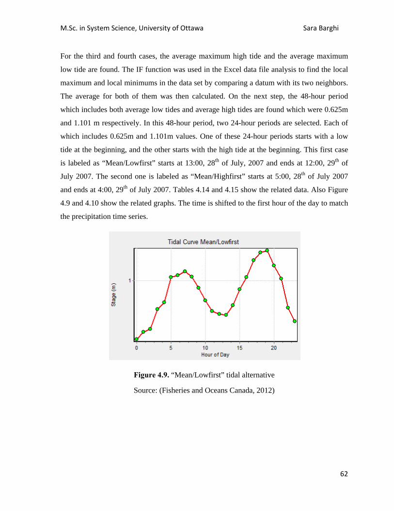
M.Sc. in System Science, University of Ottawa Sara Barghi
62
For the third and fourth cases, the average maximum high tide and the average maximum
low tide are found. The IF function was used in the Excel data file analysis to find the local
maximum and local minimums in the data set by comparing a datum with its two neighbors.
The average for both of them was then calculated. On the next step, the 48-hour period
which includes both average low tides and average high tides are found which were 0.625m
and 1.101 m respectively. In this 48-hour period, two 24-hour periods are selected. Each of
which includes 0.625m and 1.101m values. One of these 24-hour periods starts with a low
tide at the beginning, and the other starts with the high tide at the beginning. This first case
is labeled as “Mean/Lowfirst” starts at 13:00, 28th of July, 2007 and ends at 12:00, 29th of
July 2007. The second one is labeled as “Mean/Highfirst” starts at 5:00, 28th of July 2007
and ends at 4:00, 29th of July 2007. Tables 4.14 and 4.15 show the related data. Also Figure
4.9 and 4.10 show the related graphs. The time is shifted to the first hour of the day to match
the precipitation time series.
Figure 4.9. “Mean/Lowfirst” tidal alternative
Source: (Fisheries and Oceans Canada, 2012)

M.Sc. in System Science, University of Ottawa Sara Barghi
63
Table 4.14. “Mean/Lowfirst” tidal alternative
Source: (Fisheries and Oceans Canada, 2012)
Time
Level(m) Time Level(m)
00:00 0.363 12:00 0.635
01:00 0.441 13:00 0.625
02:00 0.471 14:00 0.733
03:00 0.689 15:00 0.904
04:00 0.764 16:00 1.035
05:00 1.035 17:00 1.223
06:00 1.06 18:00 1.308
07:00 1.101 19:00 1.327
08:00 1.045 20:00 1.163
09:00 0.92 21:00 1.021
10:00 0.783 22:00 0.703
11:00 0.667 23:00 0.557

M.Sc. in System Science, University of Ottawa Sara Barghi
64
Table 4.15. ”Mean/Highfirst” tidal alternative
Source: (Fisheries and Oceans Canada, 2012)
Time
Level(m) Time Level(m)
5:00 1.182 17:00 0.764
6:00 1.253 18:00 1.035
7:00. 1.28 19:00 1.06
8:00 1.239 20:00 1.101
9:00 1.029 21:00 1.045
10:00 0.893 22:00 0.92
11:00 0.6 23:00 0.783
12:00 0.494 00:00 0.667
13:00 0.363 01:00 0.732
14:00 0.441 02:00 0.635
15:00 0.471 03:00 0.625
16:00 0.689 04:00 0.733
Figure 4.10. “Mean/Highfirst” tidal alternative
Source: (Fisheries and Oceans Canada, 2012)

M.Sc. in System Science, University of Ottawa Sara Barghi
65
4.2.2.3. Initial Depth The third uncontrollable variable is the initial depth in the lower road junctions. As
mentioned in section 4.1 above, the initial depth can be 0 meaning “dry”, i.e., at the time of
starting the simulation there is no water in the junctions and storage units. The other case is
to be equal to the height of the regulators at its worst case. As mentioned in section 4.1, the
height of the regulator shows the water level that triggers the regulators to open. If the initial
depth is equal to the height of the regulators, the length of time of pumping will increase.
4.2.2.4. Impervious Percentage The fourth and the last uncontrollable variable is the impervious percentage for the lower
and the higher subcatchments. By choosing this variable as one of the uncontrollable
variables, we determine the amount of water which is assumed to flows into the sewage
system through manholes, and the amount of water which infiltrates into the ground. The
combination of the impervious percentage for the Higher Road and the Lower Road are
defined as alternatives for this variable. For example, when the High Road impervious
percentage is 25%, the Lower Road impervious percentage is set to 50%. Alternatively,
when the High Road percentage is 50%, the Lower Road percentage is set at 75%. These
different values for higher and lower impervious percentage are attributed to residential
versus undeveloped land use of each subcatchment and are estimates of parameter values for
which no empirical values are available. These estimates are assigned in order to reflect
known SWMM outcomes for historical storm events.
The historical storm event of August 26, 2010 was used throughout the simulation analysis
to help estimate these parameters by calibrating the model results under different parameter
values to the well-known storm impacts, flooding events, road closures, etc. In this manner,
validation of the simulation results was matched to the most appropriate and reasonable
parameter values in the absence of actual data.
The controllable and uncontrollable variables combined, ten scenarios are defined for the
simulation of the water system in Arichat. These scenarios are different combinations of
controllable and uncontrollable variables’ alternatives. Applying each scenario to the
developed model will result in status reports, graphs, tables and profile representations. The
application and results of each of the scenarios are discussed in Chapter 5.

M.Sc. in System Science, University of Ottawa Sara Barghi
66
5. Results and Analysis Chapter 5 contains three (3) main sections, namely: (5.1) Simulation Design; (5.2) Scenario
Results; and (5.3) Analysis of the Results. In this chapter, ten simulation scenarios, their
definitions and their inputs are discussed in 5.1. Results achieved from the simulation of
these scenarios are discussed in section 5.2. Simulation run for each scenario results in
different outputs. These outputs are analyzed in order to investigate the system’s capacity,
and to consider water quality (section 5.3).
5.1. Simulation Design Based on the controllable and uncontrollable variables introduced in Chapter 4, different
scenarios can be investigated with the combination of alternatives of controllable and
uncontrollable variables for the purpose of this research. In this research 10 scenarios are
introduced. Each scenario focuses on one or two of the variables. The objective is to use the
SWMM simulation model to investigate the water quality and the capacity of the Arichat
water system under alternative setting for the controllable and uncontrollable variables. With
regard to water quality, the amount of untreated water entering the harbor is a factor that
should be considered. Also, the number of junctions and storage units getting flooded is also
a factor for analyzing and understanding the limits of the system’s capacity. Table 5.1
presents the definitions of the 10 simulation scenarios of this analysis. Each scenario is
discussed in more detail below.
5.1.1. Status Quo Scenario The Status Quo (SQ) scenario is the first scenario of Table 5.1 and is considered as the
benchmark scenario of the simulation model. Results of all other scenarios are compared to
the results of this benchmark or “base case” scenario to investigate their differences. The
Status Quo scenario definition is given in Table 5.1 by the variable values as follows:
• Regulators (designated in the model as R1 to R6, see also section 4.1.6 above) are
denoted as the controllable variables of the simulation. For the Status Quo scenario,
all Regulators are open, based on the control rules discussed in Chapter 4 as one of
two alternatives for regulators’ status.

M.Sc. in System Science, University of Ottawa Sara Barghi
67
Table 5.1. Simulation design:Scenarioes description
Scenarios
Variables
1 SQ
2 Best Case
3 Worst Case
4 Precipitation
Focus
5 Tide Focus
6 Tide & Initial Depth Focus
7 Regulators
& precipitation Focus
8Tide &
Impervious% Focus
9 Depth & precipita-
tion Focus
10 Depth
& Impervious%
Focus
Controllable Variable
Regulators (R1-R6) Open Closed Open
Open
Open
Open
Closed Open Open Open
Uncontrollable Variable
Precipitation (mm) Off Off P3 P3 Off
P1
P3 P2 P3 P3
Tidal Level(m) Mean/Low Low High Mean/Low High High Mean
/Low High Mean /Low
Mean /High
Initial Depth(m) 0 0 2.591 0
0
2.591 0 0 2.591 2.591
Impervious percentage
(Higher Road Catchments)
25% 25% 50% 25%
25%
25% 25% 50% 25% 50%
Impervious percentage
(Catchments between higher and lower Road)
50% 50% 75% 50%
50% 50% 50%
75% 50% 75%

M.Sc. in System Science, University of Ottawa Sara Barghi
68
• With respect to the uncontrollable variables for the Status Quo, Precipitation is at its
lowest value which in this case designated as “Off” for the precipitation variable, i.e., the
minimum (0.3mm per hour) rain or snow is recorded for this case.
• The Status Quo Tidal level as noted in Table 5.1 is set at an intermediate level. In this
case, tides are designated as “Mean/Low”, which is the representation for the tidal level
time series containing the mean historical value starting with low tide.
• The initial depth of the junctions and storage units is set equal to 0 meters. Zero means
that there is no water in the system at the beginning point of the 24-hour simulation.
• The last variables are the impervious percentages for the subcatchments above the High
Road, and the impervious percentage for the subcatchments between the High and Lower
Roads. For the Status Quo scenario, these values are set at 25% and 50% respectively.
These choices help to guide less water into the system in comparison with alternative
impervious percentages for the subcatchments. These percentages are not based on
empirical valuation, but are simple estimates of water entering the sewage system
through the catchments.
5.1.2. Best Case Scenario The Best Case scenario is that case in which less water is present in the system (from
uncontrollable variables) and untreated water does not flow into the harbour. Also, Best Case is
considered as such since it has a minimum number of junctions getting flooded and the number
of hours of flooded junctions is negligible. Therefore, to define this scenario, all Regulators’
control rules are set on “close” at all times, and water is prevented from flowing directly into the
ocean and harbor, except through the treatment plant outfall and after flow-through aeration and
scrubbing of ejected water. Low precipitation is considered for the system as “Off” (Table 5.1).
The level of tides for this case is set at its lowest historical level, i.e., the “Lowest Low” tidal
level is used for the Best Case definition (Table 5.1). The Initial depths of the junctions and
storage units are set at zero, and the impervious percentages for subcatchments are at their lowest
assumed values (25% for High Road subcatchments, and 50% for Lower Road subcatchments).
This situation applies less pressure to the system and reduces the probability of flooding
junctions.

M.Sc. in System Science, University of Ottawa Sara Barghi
69
5.1.3. Worst Case Scenario The Worst Case scenario is the opposite of the Best Case. In this case, it is assumed that
untreated water may enter the harbour and the number of junctions flooded and duration of
flooding is high. In order to define this scenario, the Regulators are “Open” when the depths of
storage units get to a specific depth (2.591 meters), which is the height of the Regulators, and the
height of the outflow of the storage units (Table 5.1).
For Precipitation, the time pattern “P3” is chosen. P3 precipitation has the highest amount of
rainfall in the first 4 hour period of the 24 hour simulation (refer to section 4.2.2.1). This
significant precipitation places high pressure on the system from the beginning of the simulation.
The Worst Case Tidal level is set as the “Highest high tide” that places further pressure on the
junctions and outfalls of the system. Consequently, the model shows that initially, due to the tidal
pressure, there will be a flow from the harbour back into the system. Initial depth is also
considered at its highest value, which is equal to 2.591 meters as explained in Chapter 4, section
4.2.2.3. The impervious percentages are considered at their highest values that effectively puts
more water into the system which are 50% for the highest subcatchments, and 75% for the lower
subcatchments. By choosing these percentages, less water is assumed to infiltrate into the ground
and more water will flow into the sewage system junctions.
5.1.4. Precipitation Focus Scenario This Precipitation Focus scenario focuses on the singular impacts of significant precipitation on
the system. All the variables except the precipitation have the same values as the “Status Quo”
scenario described above. The results of this scenario will be compared directly with the result of
the Status Quo scenario and the differences in attributed to the significant precipitation. To
define this scenario, the precipitation variable (P1, P2, or P3) were considered. The scenario was
examined 3 times and each time precipitation case results among “P1”, “P2” and “P3” compared.
Then, the simulation that showed the highest incidence of junctions flooded and the release of
more untreated water flowing directly into the harbor is considered as the most significant
precipitation case for defining the Precipitation Focus scenario. The most significant
precipitation variable on the water system was found to be P3 which resulted in 5 flooded nodes
compared with no flooded nodes for P1 and P2 precipitation variables in their results. The

M.Sc. in System Science, University of Ottawa Sara Barghi
70
simulation is run under the situations for the precipitation focus scenario considering P3 as the
precipitation alternative for the Precipitation Focus scenario.
5.1.5. Tide Focus Scenario In the Tide Focus scenario, the focus is on the tidal level. For this case, all other variables are set
to have the same values as the SQ scenario with the exception of the tidal level variable. This
scenario aims to analyze the effects of alternative tidal levels on the system. For the tidal level in
this scenario, the same process for choosing the most significant precipitation variable is applied
to find the most significant tidal level among the 4 tidal cases, namely: “High”, “Low”,
“Mean/Low” and “Mean/high” tides. Running the simulation model under the different tidal
level time series shows that none of the tidal cases result in flooded junctions, but the simulations
with “High” tide time series results in surcharging 6 junctions. Thus, the most significant tidal
level is designated as the “High” tidal level time series, and is chosen for this scenario for the
tidal level alternative.
5.1.6. Tidal Level and Initial Depth Focus Scenario This scenario focuses on the tidal level and the initial depth of the junctions at the same time.
The precipitation case for this scenario is set as “P1”, corresponding to the historical time series
for the August 24, 2010 storm that happened in Arichat area (Environment Canada, 2012). The
tidal level here is considered as the most significant tidal level which is defined in section 5.1.5
above (i.e., “High” tide) to represent the focus of this scenario for the tidal level. The initial
depth is the highest one, namely 2.591 meters to show the focus on the initial depth. Finally,
impervious percentages and regulators status remain the same as the Status Quo scenario as
noted in Table 5.1.
5.1.7. Regulators and Precipitation Focus Scenario The Regulator and Precipitation Focus scenario is a scenario with focus on the variables for
regulators (controllable) and precipitation (uncontrollable). For this scenario, the regulators are
kept closed throughput the simulation thereby preventing the release of untreated water into the
harbour. For precipitation, as investigated in section 5.1.4 above, the most significant
precipitation case is P3. The remaining scenario variables for tidal level, initial depth and
impervious percentages are set the same as for the SQ scenario defined in 5.1.1 above (Table
5.1).

M.Sc. in System Science, University of Ottawa Sara Barghi
71
5.1.8. Tidal Level and Impervious Percentage Focus Scenario The Tidal Level and Impervious Percentages Focus scenario defines the most significant tidal
level and the highest variable values for the impervious percentages. Therefore, the tidal level is
set as the “High” tidal level time series. For this scenario, the impervious percentages are 50%
for the higher subcatchments and 75% for the lower subcatchments. “P2” is the precipitation
case for this scenario. The Initial depth of junctions is set at 0, the same as the SQ scenario, and
regulators are “Open” in the simulation of this scenario. This scenario is designed to investigate
the significance of the combined tide and runoff to the water system.
5.1.9. Initial Depth and Precipitation Focus Scenario This Initial Depth and Precipitation Focus scenario combines the effects of the initial depth of
the junctions, and the precipitation uncontrollable variables on the system. The difference
between this scenario and SQ scenario is in the Initial Depth values which are set at the highest
level of 2.591m here. The Precipitation case that is judged to be the most significant precipitation
is found in section 5.1.4 and denoted as P3. The rest of the variables are the same as the SQ
scenario (Table 5.1): Regulators are open throughout the simulation time period (24 hours);
Impervious percentages for the higher and lower subcatchments are 25% and 50%, respectively;
and, the tidal level is the mean tidal level time series starting with a low tide at the beginning of
the simulation time (“Mean/Low”).
5.1.10. Initial Depth and Impervious Percentage Focus Scenario The last scenario defined for the purpose of this research is the Initial Depth and Impervious
Percentage Focus scenario. This scenario focuses on the initial depth of the junctions and the
impervious percentage of the subcatchments. This scenario is comparable with “Precipitation
Focus” scenario. For this scenario, regulators are open during the simulation. The precipitation
case is “P3 “which is the most significant precipitation variable. This precipitation case is chosen
the same as Precipitation Focus scenario of 5.1.4 above. The tidal level is set at the mean tidal
level time series starting with a high tide. The Initial Depth of the junctions is set at the high
level of 2.591 meters as the focus is on the initial depth. The Impervious Percentages are set at
high levels of 50% and 75% for the higher subcatchments and the lower subcatchments,
respectively. Comparing this scenario with the “Precipitation Focus” scenario results in finding
effects of Initial Depth and Impervious Percentage focus on the system (Table 5.1).

M.Sc. in System Science, University of Ottawa Sara Barghi
72
5.2. Scenario Results In this section the simulation model results for each scenario are presented and discussed.
Related graphs and tables for all model results are found in Appendix C – “Simulation Model
Simulation Scenario Results”. As mentioned in the previous section, the results for all the
scenarios are compared with the benchmark case, the SQ scenario. SQ results are discussed fully
in the next section and the results for all other scenarios are presented in comparison of the
scenarios’ results with SQ results presented below in 5.2.1.
5.2.1. Status Quo Scenario Results The model simulated as the Status Quo scenario is defined in section 5.1.1 above. Tables C.1 to
C.21 in Appendix C presents the status report for this scenario.
Continuity Errors. The first result of the SWMM simulation model that is shown after simulation
run is the SWMM model continuity errors, i.e., the continuity error for (i) surface runoff, (ii)
flow routing and (iii) quality routing for the 24 hour simulation period. The SQ scenario results
are (i) -0.06%, (ii) 1.6% and (iii) -1.52%, respectively for the continuity error set. As discussed
in Chapter 3, Section 3.4, when the continuity error is less than 10%, it is considered as
“acceptable”. In the status report for the SQ scenario results, which is provided in Appendix C,
Section C.1 – “Status Quo Scenario Simulation Status Report”, the continuity error for junctions
with the highest error is recorded. Based on the SQ scenario results, the errors are under 10% for
all the junctions. Thus, all continuity errors for the SQ are in an acceptable range.
Subcatchment Reports. In the subcatchment runoff summary of this report for the SQ
benchmark scenario, the results show that the total precipitation for all the subcatchments is
equal as they receive the precipitation from the same rain gauge (Gauge 1, Figure 3.11). Each
subcatchment’s total infiltration is calculated based on the impervious percentage for each
subcatchment area. For example, for the S1 subcatchment (Figure 4.2), the total infiltration value
is equal to 25% of the total precipitation value for S1.
The status report on the “Subcatchment Washoff Summary” provides the estimated amount of
pollutants that are washed off each subcatchment into the system. Each of the subcatchment
estimates is calculated based on the land use percentages provided in the subcatchment
properties (Table 5.1). The smaller the residential percentage provided for a subcatchment, the

M.Sc. in System Science, University of Ottawa Sara Barghi
73
fewer amount of pollutants are washed off into that subcatchment. Also, the area of the
subcatchment has an impact on the amount of wash-off in a subcatchment. More pollutants are
washed off from the subcatchments to the system when the area of a subcatchment is larger.
These washoff values include the “Total Soluble Solids”, TSS, and Lead as the standard
pollutants. Model estimates for TSS and Lead are calculated based on the EMC (Event Mean
Concentration) function which is defined in the SWMM model for these pollutants. The values
for Lead are 0.25% of the value of TSS because Lead is defined as the co-pollutant for TSS with
the 0.25 as the fraction value. This value is provided in the SWMM manual water quality
example which is used for the purpose of this research.
Node Depth Summary. The “Node Depth Summary” of the SWMM results for the SQ scenario
shows the average depth summary, the maximum depth, maximum HGL (Hydraulic Grade Line)
and the time of maximum occurrence. Discussing these values is important whenever a junction
gets surcharged or flooded. In the SQ scenario, none of the junctions and storage units is flooded
or surcharged. The reason for this is because of the precipitation and the choice of tidal level in
this scenario. The precipitation value is low and the tidal level has a medium level. Therefore,
the average depth in the water system is not high for most of the junctions and represents a base
validation of the model under these circumstances, as expected. This value for the Outfalls are
higher than other junctions because of the tidal level which has effects on the level of water in
the outfalls and water in the system flows into these outfalls whenever the control rules for the
valves become true and the valves are opened. For all the outfalls and all the junctions connected
to the outfalls, the maximum depth occurs at the same time that the tidal level is at its highest
value. At 19:00(7:00pm) the value of the tidal level time series starting with a low tide is 1.327
meters based on Table 4.14 and Figure 4.9. Figure 5.1 shows all outfalls depths change during
the time of the simulation. The graph of Figure 5.1 follows the same pattern as the tidal level
graph which is presented in Figure 4.9. This is evidence, as expected, that the maximum rates for
the outfalls and junctions connected to outfalls are at the same time the highest tidal level.

M.Sc. in System Science, University of Ottawa Sara Barghi
74
Figure 5.1.Outfalls Depth
Node Inflow Summary. The Node Inflow summary represents the amount of water that flows into
each junction. Junction can have inflows from different resources. These resources can be
external or internal. In the node inflow table, maximum lateral inflow is the inflow from external
sources shown for each junction. External sources are inflows from subcatchments which enter
the junction. For junctions j7, j9, j11, j12, j14, TPO (TreatmentPlantOutfall) (Figure 4.2) and all
the outfalls (Outfall1 through Outfall6), the lateral inflow volume is 0mm as these nodes are not
connected to any subcathment. Other junctions have lateral inflows as they are connected to
subcatchments. The volume of lateral inflow for these junctions is dependent on the area of the
subcatchment and the impervious percentage of each subcatchment. This table also presents each
junction’s maximum total inflow and shows the time of the maximum occurrence. The total
inflow volume values in this table are 0 mm for j7 and j14. The reason is that the pumping
summary table at the end of the status report in Appendix C (Table C.21) shows that pump p1
and pump p2 have never started up during the SQ benchmark simulation. This means that there
is no water pumped up to j7 and j14 during the simulation.
Surcharged and Flooded Nodes. The SQ benchmark simulation model report on surcharged and
flooded nodes show no junction or storage unit as surcharged or flooded (Tables C.14 and C.15)
and This means that in the absence of significant precipitation and with a mean value for tidal
level as inputs for the SQ benchmark scenario the capacity of this system is sufficient to deal
with this case.

M.Sc. in System Science, University of Ottawa Sara Barghi
75
Outfall Loading. The “Outfall Loading” table shows the results related to the flow through the
six outfalls in the model for the SQ scenario. The results show the ‘flow frequent percentage’ or
the percentage of time that there is a flow in these outfalls as water released to the harbour. For
most outfalls, this percentage is close to 100%. The flow in most of the outfalls is attributed to
the tidal level. The total volume of water in the outfall connected to the treatment plant (TPO,
Figure 4.2) is higher than other outfalls as it is the very last outlet of the system and all the water
in the system is guided to this outfall through the pipes in the system and treated before releasing
to the harbour. This table also presents the amount of TSS and Lead which flow into these
outfalls as estimated parts of untreated water. Treatment plant outfall has the lowest value for
TSS which is expected since untreated water gets treated at this outfall, therefore it is assumed
that treated water (aerated and scrubbed) has less TSS. Other outfalls (with the exception of
Outfall4) have higher values for TSS as the water flows to these outfalls is not treated, therefore
it is assumed to contain a higher level of TSS and Lead pollutants. Outfall4 does not have any
value for TSS as all the water containing TSS flowed into the treatment plant and was treated
there (through aeration and scrubbing); therefore, no water flows into Outfall4. Outfall4 is a
support outfall for the treatment plant, in the case that the depth of the treatment plant node
exceeds to 2.591 meters, regulator R4 is opened and untreated water flows into this outfall. Table
5.2 compares outfall3, TPO and Outfall2 TSS values. As it is obvious in the graph Outfall2 and
Outfall3 in some parts of the day have high values for TSS, this is because of an assumption in
SWMM modeling system. This assumption considers that the time people generally get up –
around 7-10am, and when families go to bed – around 9-11pm, i.e., when they tend to emit
sewage flow (this timing is shown in the graph). In compare to j10, j8 is connected to larger
subcatchments and that causes more sewage be released into Outfall2 in compare to Outfall3.
Figure 5.2. TSS values in Outfall2, Outfall3 and TPO

M.Sc. in System Science, University of Ottawa Sara Barghi
76
Pumping Summary. The last output table of interest is the pumping summary table. For the SQ
scenario, p1 and p5 have not started up during the simulation. This is because in the node depth
summary table, the value for the maximum depth of nodes j6 and j15 which are connected to
these to pumps are 0.96 meters and 1.56 meters, respectively. On the other hand, based on
Chapter 4 description the startup depth for both of the pumps p1 and p5 is 1.829 meters.
Comparing nodes depth and the pump start up depth, it is understood why these pumps have not
started up during the simulation. On the other hand, the other pumps p2, p3, and p4 have
maximum depths higher than their pump start up depth; therefore, they have started up once time
during the simulation. As well, the “Node Inflow summary” table referred to above, the inflow
for j6 and j15 is less than other junctions. Moreover, among the other 3 junctions which are
connected to other pumps, j8 has the lowest inflow volume. This means that pump p2 was
working for less time (20.91%) in comparison with the other 2 pumps, p3 (85.29%) and p4
(80.4%) which have higher inflow volume over the 24 hours of the simulation period.
In order to analyze the whole system, Figure 5.3 shows the total inflow and outflow of the
system during the 24-hour simulation. From this graph, it is obvious that whenever inflow is high
outflow is low. Inflow starts from a high value because based on the “OFF” case for the
precipitation, which is the input for SQ scenario, from the first moment of the simulation there is
a precipitation in the system with 0.3mm as the value. One of the sources of inflow to the system
is tidal level time series, which is the most effective one in SQ scenario as precipitation is at its
lowest value for this scenario.
Figure 5.3. System Total Inflow and Outflow for SQ Scenario
In Figure 5.3, the red line shows the total inflow in this graph. Comparing this line with Figure
4.9 which is the graph for “Mean/Low” tidal level, the total inflows follow the same pattern as
the tidal graph of Figure 4.9. The green line shows the outflow of the system, and although it is
lower than the red line in some parts, it is increasing during the simulation time; this is because
anyway water has to leave the system at any moment of the simulation. Therefore, the outflow
graph is an ascending graph.
Table 5.2 represents a summary on the SQ scenario results.
Figure 5.3. System Total Inflow and Outflow for SQ Scenario

M.Sc. in System Science, University of Ottawa Sara Barghi
77
In Figure 5.3, the red line shows the total inflow in this graph. Comparing this line with Figure
4.9 which is the graph for “Mean/Low” tidal level, the total inflows follow the same pattern as
the tidal graph of Figure 4.9. The green line shows the outflow of the system, and although it is
lower than the red line in some parts, it is increasing during the simulation time; this is because
anyway water has to leave the system at any moment of the simulation. Therefore, the outflow
graph is an ascending graph.
Table 5.2 represents a summary on the SQ scenario results. It shows average number of hours
junctions are flooded or surcharged. Also it shows average flow for outfalls in CMS (Cubic
Meter per Second) and the same value is shown for TPO (TreatmentPlantOutfall). TSS and Lead
values are also shown in kg in this table. Pumps information, the utilization percentage and the
number of startups are also shown as important results in this table.
Table 5.2. Status Quo Scenario Simulation Results Summary
Scenario
Average
Number of
Flooding
Hours
Average
Number of
Surcharging
Hours
Average
Flow for
TPO
(CMS)
Average Flow for System’s
Outfalls(CMS)
Total TSS in TPO(kg)
Total TSS Loaded to
the Outfalls(kg)
Total Lead
in TPO (kg)
Total Lead
Loaded to the
Outfalls(kg)
Pumps Working:
The Percentage of
Each Working,
Number of Start
ups
SQ
Scenario --- ---
0.12
0.388
TPO:1.201
56.217
TPO:0.015
0.029
P1: 0%,0
P2:80.4%, 1
P3:85.29%,1
P4:20.91%,1
P5:0%,0
5.2.2. Best Case Scenario Results The model is simulated under best case scenario conditions discussed in section 5.1.2. Tables
C.22 to C.42 in section C.2 of Appendix C present the status report for this scenario.
The best case scenario continuity errors for surface runoff, flow routing and quality routing are:
0.06%, 1.00% and -5.51%, respectively. The error values are all less than 10%, so they are in the
acceptable range. In the status report for this scenario, junctions j6, j13 and j8 have continuity
errors which exceed 10%. If these junctions are found important for the purpose of the research
then their continuity error should be reduced. As there are no junctions flooded or surcharged in
this simulation scenario, it is assumed that there is no need to be concerned about these junctions.

M.Sc. in System Science, University of Ottawa Sara Barghi
78
In comparison to the Status Quo scenario, the Best Case “Runoff Summary” is not different. This
is because the precipitation case is the same for both of these scenarios and that is why all the
subcatchments in this scenario receive the same amount of water as the SQ benchmark scenario.
Similarly, the “Subcatchment Washoff Summary” table is the same as that for the SQ scenario
results. This is again because of the same inputs for the precipitation and the same example used
for the pollutants.
In the “Node Depth Summary Table”, the Best Case depth of junctions on the High Road is the
same as the corresponding values in the SQ scenario results. The value for the “TreatmentPlant”
junction depth is less than what resulted in SQ scenario node depth table. Also, for j7, j9, j11,
j12and j14, the average depth is 0. The reason for having these results is that by closing the
regulators in the system the effect of tides on the junctions connected to the outfalls will be
eliminated. Tides only have effects on the outfalls and there is no way for them to connect to the
system. Therefore the depth of the water in junctions j6, j8, j10, j13 and j15 are less than what is
recorded in the SQ scenario, and also are less than the startup depth of the pumps. Therefore, the
model pumps never start up and do not lift water up to the pumps’ outlet junctions which are j7,
j9, j11, j12and j14. That is why these junctions never have any water available in them. All these
values result in lower depth in the “TreatmentPlant” junction. Also, it causes lower values as the
depth for outfall junctions. Comparing maximum depth for the outfall with the maximum value
in the “Low” tidal level time series in Figure 4.8 and Table 4.13 shows that outfall depths are due
to low tidal level time series in Best Case Scenario. For all the outfalls, the maximum depth
happened at 10:00am and the highest tide in the lowest low tidal level time series happened
exactly at 10:00am with 1.166 meters as the value.

M.Sc. in System Science, University of Ottawa Sara Barghi
79
Figure 5.4. Outfall Depths for Best Case Scenario
Figure 5.4 shows all the outfalls’ depth during the 24-hour simulation under Best Case scenario
inputs. Some hours of the day depth of the nodes are 0, the reason is that in some hours of the
day the tidal level is negative or 0 so it does not have any impact on the depth of the outfalls.
Based on the explanation above, the Best Case inflow for the junctions on the High Road
remains the same as the SQ scenario result, as these junctions receive the same precipitation as in
the SQ scenario. Treatment plant inflow is lower than the SQ scenario as no water is lifted up to
outlets of the pumps, and therefore the inflow source from these outlets is not considered for the
treatment plant. Outfalls do not have any inflow as the regulators connected to these outfalls are
closed based on the inputs for the Best Case scenario.
No junctions are flooded or surcharged in the Best Case simulation, as expected, which is the
same as for the SQ scenario results for flooding and surcharging.
Outfall loading summary for the Best Case scenario shows that only the “TreatmentPlantOutfall”
has loadings during the simulation. This is because of the closed regulators status that does not
let water flow into outfalls from storage units. Also, the amount of TSS in this outfall is very
small, although the total amount of TSS in the system (based on the “washoff results” table) is
193.21 kg. This happens because the water remains in the storage unit till it is lifted up with the
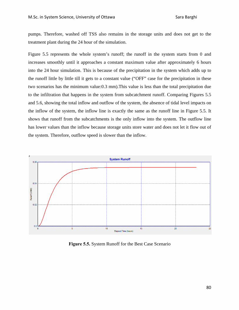
M.Sc. in System Science, University of Ottawa Sara Barghi
80
pumps. Therefore, washed off TSS also remains in the storage units and does not get to the
treatment plant during the 24 hour of the simulation.
Figure 5.5 represents the whole system’s runoff; the runoff in the system starts from 0 and
increases smoothly until it approaches a constant maximum value after approximately 6 hours
into the 24 hour simulation. This is because of the precipitation in the system which adds up to
the runoff little by little till it gets to a constant value (“OFF” case for the precipitation in these
two scenarios has the minimum value:0.3 mm).This value is less than the total precipitation due
to the infiltration that happens in the system from subcatchment runoff. Comparing Figures 5.5
and 5.6, showing the total inflow and outflow of the system, the absence of tidal level impacts on
the inflow of the system, the inflow line is exactly the same as the runoff line in Figure 5.5. It
shows that runoff from the subcatchments is the only inflow into the system. The outflow line
has lower values than the inflow because storage units store water and does not let it flow out of
the system. Therefore, outflow speed is slower than the inflow.
Figure 5.5. System Runoff for the Best Case Scenario

M.Sc. in System Science, University of Ottawa Sara Barghi
81
Figure 5.6. System Total Inflow and Outflow for the Best Case Scenario
Table 5.3 represents a summary on the results of the Best Case scenario. As explained above, the
Best Case scenario is considered as “best” because it controls the release of untreated water
through the outfalls so that less pollutant enter the harbour. This scenario in comparison with the
SQ scenario reduces the amount of TSS and Lead entering the harbour. Comparing the summary
results of the two scenarios shows this difference. In the SQ scenario, all the outfalls have high
values for the TSS and Lead which enter the harbour directly. In the Best Case scenario, the
summary results show that only the treatment plant outfall releases TSS into the ocean. The
amount of the release of treated water (aerated and scrubbed) is only 0.013kg, which is a small
number in comparison with the total TSS loading into outfalls in the SQ scenario.
Table 5.3. Best Case Scenario Result Summary
Scenario
Average
Number of
Flooding
Hours
Average
Number of
Flooding Hours
Average
Flow for
TPO
(CMS)
Average Flow for System’s
Outfalls(CMS)
Total TSS in TOP (kg)
Total TSS Loaded to
the Outfalls(kg)
Total
Lead in
TPO (kg)
Total Lead
Loaded to
the
Outfalls(kg)
Pumps Working:
The Percentage of
Each Working,
Number of Start
ups
Best
Case
Scenario
--- ---
0.01
0.01
0.013
0.013
TPO:0.0
0.01
P1:0%,0
P2:0%,0
P3:0%,0
P4:0%,0
P5:0%,0

M.Sc. in System Science, University of Ottawa Sara Barghi
82
5.2.3. Worst Case Scenario Results The model simulated as the Worst Case scenario is defined in section 5.1.3 above. Tables C.43 to
C.63 in part C.3 of Appendix C present the status report for this scenario.
. The continuity error for surface runoff, flow routing and quality routing are acceptable: 0.04-%,
-0.1% and -0.1%, respectively. Junctions j7 and j14 have the highest continuity error but these
values are also less than 10%.
As discussed in section 4.2.2.1, the total amount of the highest level of precipitation, P3 is
86mm. This value is the exact value shown in the runoff summary table in the status report of the
simulation for the Worst Case scenario. The infiltration value for subcatchments in this scenario
is less than the SQ scenario because of the higher impervious percentage for each subcatchment.
This results in more inflow into the Worst Case scenario system results.
The “Washoff Results” table shows a larger number as the total amount of TSS and Lead in the
system compared to the SQ benchmark results. This is because of highest values for the runoff
which cause washing more TSS and Lead into the system. The highest the runoff is, the more
pollutants is washed from the subcatchments into the system.
In the “Node Depth Summary Table”, it is shown that junctions on the High Road have higher
depths in this scenario in comparison with the SQ scenario because they receive more runoff
from the subcatchments. The Treatment plant junction has a value for this simulation which is
also higher than the value in the SQ scenario simulation. This is again because of the higher
values for the precipitation time series and also because of the choice of highest high tide for all
the outfalls. And, as all the water in the system aims to get to the treatment plant as the final
destination, the value for the depth and volume of the “TreatmentPlant” junction is higher than
other junctions in the system. However, the “TreatmentPlantOutfall” depth has a lower value
than the “TreatmentPlant” junction. This means that some part of the water flowed into
“Outfall4” because the maximum depth in the “TreatmentPlant” is 8.38 meters. This value
shows that the regulator R4 was open at sometime during the simulation because 8.38 meters is
higher than the 2.591 meters the control level rule that opens R4 so that untreated water can flow
into the Outfall4. Also, because of the initial depth value for the Lower Road junctions, they
mostly have a high maximum depth and the average depth for the junctions in this simulation is

M.Sc. in System Science, University of Ottawa Sara Barghi
83
higher than the comparable SQ result. Most of the maximum depths for the junctions occured
during the first hours of the simulation. This due to the front loaded time series of heavy
precipitation. The first 4 hours of this time series have the highest precipitation value as WOrst
Case loading. The rest of the time,precipitatin is 0mm.
Figure 5.7 reflects the same concept for the storage units in the system. The first 4 hours of the
simulation, because of the high precipitation value, the depth of junctions are increasing. Each
junction depth starts from the initial depth (2.591 meters) and goes up to a maximum level, This
maximum level is dependent on the area of the subcatchments conncted to these junctions. After
this maximum level is achieved, the depth decreases since the precipitation decreases to zero for
the rest of the simulation and since then the only inflow into the system comes from the high
tidal level. The second reason is because of the control rules on the regulators. Regulators
become open when the depth of the storage unit connected to them gets more than 2.591 meters.
As in Figure 5.7, all the storage units’ depths are higher than 2.591 meters at the beginning of the
simulation because of the initial depth consideration for this scenario. After this depth is attained,
the regulators are opened and the pumps are all working causing the depth in the nodes to
decrease. Since then, the graphs are following the same shape as the high tide time series which
is shown in Figure 4.7. Regulators are closed after a reduction in the junctions’ depth and when
depths get to 1.829 meters, the pumps start working. For some junctions, e.g., j13, j10 and j8,
their depth is always higher than 1.829 meters (for j13 and j8) and for j10 higher than 1.524
meters (which are the startup depths of the pumps connected to these junctions). These pumps
work 100% of the time.

M.Sc. in System Science, University of Ottawa Sara Barghi
84
Figure 5.7. Storage Units Depth in Worst Case Scenario
Figure 5.8 shows similar trajectories for the outlet junctions of the pumps in the Worst Case
scenario as in Figure 5.7. The same process is occurring for these junctions. Junction j14 depth
increases and then decreases to zero. Pump p1 works only for 38% of the time and that is
because of what is obvious in Figure 5.7, i.e., the depth of the j15 most of the time is less than
the 1.829 meters therefore the pump needs only to start up only once and then shut off soon after
because the depth decreases to the shut off depth (1.219 meters).
Figure 5.8. Pumps Outlet Junctions and Treatment Plant Depth in Worst Case Scenario

M.Sc. in System Science, University of Ottawa Sara Barghi
85
Figure 5.9 shows the outfall depths and as seen in the Figure 4.7, the shapes of these graphs
follow the same relative trend as the high tide graph. Comparing Figure 5.7 and Figure 5.9, when
the depth of a storage unit is less than others, the depth of the outfall connected to the storage
unit is smaller in comparison with others. An example can be j6 and outfall1.
Figure 5.9. Outfall Depths in Worst Case Scenario
For the Worst Case scenario node inflow summary results, the “TreatmentPleant” has the highest
inflow as all the water in the system aims to flow into the treatment plant. “Outfall4” and
“TreatmentPlantOutfall” have almost the same inflow, this is because of the high depth for
“TreatmentPlant” which cause R4 to be open at some point in time and water flows into the
harbour untreated. Other outfalls also have high values for inflow, which is one of the reasons
that this scenario is labeled as the Worst Case scenario. This high value for inflows also shows
the amount of untreated water that flows into the harbour without getting to the treatment plant.
This causes more TSS and Lead to enter the harbour water.
The surcharge summary table for the Worst Case shows the junctions which are surcharged
during the simulation. Because of the initial depth in the system, most of the junctions on the
Lower Road are surcharged for at least one hour. j11 is surcharged for 11.11 hours because the
surcharge depth for this junction is lower than other junctions. Figure 5.8 shows that its depth
was almost higher than all of the other junctions. Other junctions have a reasonable number of
hours surcharged. The “Node Flooding Summary” shows that j6, j7, j8, j9, j10, j11, j12, j14, j15
M.Sc. in System Science, University of Ottawa Sara Barghi
86
and the Treatmentplant are flooded in the Worst Case scenario. Junctions j9, j7, j12 and j14 are
flooded for a neglectable number of hours (0.01 hours), and also the flooding volume is 0 liter
for all of them. The “TreatmentPlant” junction is flooded for 2.49 hours with a small amount of
flooding volume which is 0.697 (10^6) liters. This means that the capacity of the treatment plant
in this system is not enough to manage the Worst Case scenario. With this high precipitation and
high tide level the treatment plant gets flooded and untreated water flows out of the treatment
plant outfall. This untreated water might flow back into the system, infiltrate into ground or flow
into the ocean. Junction j10, the inlet of the largest pumping station (p3) is flooded for 1.21 hours
with 1.65(10^6 liters) as the flooding volume. Both of these numbers are negligible in
comparison to junctions j6, j8 and j15 which have flooding volumes equal to 8.859(10^6 liter),
5.257(10^6 liter) and 6.283(10^6 liter) respectively. The 3 pumping stations connected to these
junctions are likely to be flooded in huge storms and high tide levels (Boudreau, 2013).
The last table for the Worst Case scenario is the “Outfall Loading Summary” table. Almost all
the outfalls flow frequency percentage is 100%. Total volume for “TreatmentPlantOutfall” is
higher than other outfalls, as expected. This means that there were lots of TSS and Lead entering
the harbour from all other outfalls in the system. The proof of this is the values in this table
related to total TSS and Lead in these outfalls. Outfall5 is connected to S12 and S11. Both of
these subcatchments are highly residential which explains why although the Outfall5 loading is
almost the same as other outfalls while the amount of pollutants is higher than others. The same
reasoning is right for Outfall6 which is connected to the highly residential subcatchment S13.
In comparison with the SQ scenario and the Best Case scenario, the Worst Case scenario
experiences considerable flooded and surcharged junctions. Also, the Worst Case scenario
releases more untreated water into the harbour due to the insufficient capacity of the treatment
plant and the pumping stations to manage the high volume of water. Table 5.3 represents the
summary results for the Worst Case Scenario.

M.Sc. in System Science, University of Ottawa Sara Barghi
87
Table 5.4. Worst Case Scenario Results Summary
Scenario
Average
Number of
Flooding
Hours
Average
Number of
Surcharging
Hours
Average
Flow for
TPO
(CMS)
Average Flow
for System’s
Outfalls(CMS)
Total TSS in TPO (kg)
Total TSS Loaded to
the Outfalls(kg))
Total
Lead in
TPO(kg)
Total Lead
Loaded to the
Outfalls(kg)
Pumps
Working: The
Percentage of
Each Working,
Number of
Start ups
Worst
Case
Scenario
(11
junctions)
1.94
(10 junctions)
6.45
0.405
2.805
36.229
4658.107
0.151
1.307
P1:84.35%,2
P2:100%,1
P3:100%,1
P4:100%,1
P5:38.82%,1
5.2.4. Precipitation Focus Scenario Results The model simulated as the Precipitation Focus Scenario is presented in section 5.1.4, and Table
5.1. Tables C.64 to C.83 in part C.4 of Appendix C, present the status report for this scenario.
The continuity error for surface runoff, flow routing and quality routing for this scenario are: -
%0.03, %0.24and %0.64, respectively. Continuity error values are all less than 10% and are
considered acceptable. None of the junctions have a high continuity error in comparison with the
SQ benchmark report.
The singular difference between this scenario and the SQ scenario is the precipitation time series.
For the current scenario the precipitation series is P3. The precipitation series is the same as for
the Worst Case scenario. However, the infiltration and total runoff is different because of the
different impervious percentages considered for this scenario. The runoff is higher in this
scenario than for the SQ scenario, and the resulting amount of TSS and Lead in the washoff is
also higher than the SQ benchmark scenario. S13 has the highest value for TSS and Lead
because its area is larger than other subcatchments and, because of its location, it also has a high
percentage for the residential land use.
Node depths are higher in comparison to the SQ scenario and lower in comparison to the Worst
Case scenario. The maximum depths for “TreatmentPlant”, j11, j12, j6, j8, j10, j13 and j15 are
higher than the startup depth of the pumps, and also higher than the maximum depth for the
regulators. Thus, for this simulation, the pumps are operating (i.e., all pumps are started up at

M.Sc. in System Science, University of Ottawa Sara Barghi
88
least one time over the course of the simulation time), and regulator status is “Open”. According
to Outfall Loading table, most of the outfalls were loading almost 100% of the time for this
scenario. The total flow in the outfalls is higher than the total flow in the SQ scenario because of
the higher precipitation. This scenario also results in more inflow into the system. Comparing
Figure 5.3 and Figure 5.10(below), total system inflow and outflow follow the same pattern as
the P3 precipitation case. The higher value for the precipitation focus scenario leads to total
inflow that is almost 12 CMS which is 20 times larger than the same value for the SQ scenario.
Figure 5.10. System Total Inflow and Outflow in the Precipitation Focus Scenario
Ten junctions are surcharged in the simulation of this scenario. These are: j6, j7, j8, j9, j10, j11,
j12, j13, j15 and TreatmentPlant (Figure 4.2). In comparison to the Worst Case scenario, j14 is
no longer surcharged. Other junctions, especially j11, is surcharged for fewer hours which is
attributed to the elimination of the effect of the high tide time series, and reduction in the
impervious percentage in the Precipitation Focus scenario in comparison to the Worst Case
scenario.
The Node Flooding Summary table shows that 5 junctions are flooded in this scenario. In
contrast, the SQ scenario did not have any junctions flooded or surcharged, and the Worst Case
scenario had 10 junctions flooded. In comparison to the Worst Case Scenario, the junctions: j9,
j7, j12, j14 and j10 are no longer flooded in this scenario. The first four junctions were not
flooded for a significant number of hours in the Worst Case Scenario; therefore, it is not

M.Sc. in System Science, University of Ottawa Sara Barghi
89
surprising if they are not flooded in the absence of the high level tides in this scenario. When the
focus is on the precipitation, those connections which have more lateral inflows are more
probable to get flooded; j10 only receives water from j3 which is connected to S3. The S3
subcatchment area is 24.63 ha which is not large in comparison to the total area of the
subcatchments connected to the flooded junctions. Therefore, j10 is no longer flooded. On the
other hand, j10 has a maximum depth as 4.04m and also the average depth of j10 is 2.21m,
which means that pump 3 is working most of the time, and pumps the water into j11. As the
surcharge depth of the j11 is lower than other junctions, it floods very quickly and that is the
reason that j10 is not flooded and j11 continues to be flooded. The “TreatmentPlant” receives
water from S9, S10 and S4 which is connected to j4 with j4 connected to the “TreatmentPlant”.
As noted previously, all water in the sewage system aims to reach the treatment plant for
treatment prior to being released into the harbour. Accordingly, with the high volume of water in
the system, the treatment plant floods in this scenario. Junction “j6” receives water from S7 with
14.47 ha as its area, and also from “j1” which receives water from S1 with 26.01 ha as its area.
Therefore, it receives water from a large subcatchment area and results in the junction being
flooded. The same rationale applies to j8 and j15. All the junctions flooded in this scenario are
flooded for less than two hours (Figure 5.11). As it is clear in the graph and from the node
flooding summary table for this scenario, all the junctions are flooded within the first 4 hours of
the simulation period. This is clearly a result of the P3 front-loaded precipitation of this scenario
which has its highest rainfall value in the first 4 hours of the simulated time series.
Figure 5.11. System Flooding for the Precipitation Focus Scenario

M.Sc. in System Science, University of Ottawa Sara Barghi
90
Figure 5.12 presents a profile plot for the Lower Road connections from j6 to j15. This figure is a
screenshot of the SWMM simulation model which simulates how water flows into the system
junctions. This screenshot is taken at 3:15am for this 24-hour simulation period, or 15 minutes
after the last maximum flooding event (i.e., at 3:02am j11 flooded for 0.19 hours). The time step
for this simulation is 5 minutes so no screenshot can be captured in any time between 5 minutes.
In this figure, junctions j11, j8, j6, j15 and the treatment plant are all flooded.
Figure 5.12. Profile plot for the Lower Road Connections from j6 to j15 at 3:15:00 for Precipitation Focus Scenario
As noted above, the amount of TSS and Lead flows into the outfalls is more than the amount in
the SQ scenario, but close to the amount of the Worst Case scenario. The amount of TSS and
Lead released into the ocean from outfalls connected to the flooded junctions are more than the
Worst Case Scenario. The reason for this can be found in the pumping summary table. All the
pumps are started up at least for one time based on the pumping table for the precipitation focus
scenario. P2 and P3 were working for most of the time because the flow in j13 and j10 is not so
high, but the maximum depths for both pumps are high. The pumps start up because of the high
maximum depth and because of the flow in the inlet junctions they do not stop working and
continue working in order not to let water flow out from Outfall3 into the harbor without getting
treated. Flow in j6, j8 and j15 is high and maximum depth is high as well, therefore the pump is
not enough for lift the water up and regulators become open and most of the water flows into the
harbour from the outfalls connected to these junctions. This is one of the reasons that the TSS

M.Sc. in System Science, University of Ottawa Sara Barghi
91
value (which loads to these outfalls) is higher than other outfalls, and even higher than the Worst
Case Scenario. Pumps are apparently not working properly in these stations.
The Precipitation Focus scenario has higher Total TSS and Lead values loaded into the outfalls
in comparison to the Worst Case scenario. The amount of TSS and Lead washed off from the
subcatchments for these two scenarios is the same due to the same precipitation series, P3. On
the other hand, the total runoff in the subcatchments in the Precipitation Focus scenario is less
than the runoff in the Worst Case scenario because of lower impervious percentage in the
Precipitation Focus scenario. This causes more concentration of TSS and Lean in the runoff in
the Precipitation Focus scenario. Therefore, more TSS and Lead loads to the outfalls.
Table 5.5 represents the summary of the Precipitation Focus Scenario Results.
Table 5.5. Precipitation Focus Scenario Results Summary
Scenario
Average
Number
of
Flooding
Hours
Average
Number of
Surcharging
Hours
Average
Flow
for TPO
(CMS)
Average Flow for System’s
Outfalls(CMS)
Total TSS in TPO (kg)
Total TSS Loaded to
the Outfalls(kg)
Total Lead
in TPO (kg)
Total Lead
Loaded to the
Outfalls(kg)
Pumps Working:
The Percentage
of Each Working,
Number of Start
ups
Precipitation
Focus
Scenario
(5
junctions)
1.23
(10
junctions)
4.293
0.328
2.288
29.909
4909.817
0.179
1.399
P1:39.58%,1
P2:96.45%,1
P3:95.77%,1
P4:70.12%,2
P5:41.89%,1
5.2.5. Tide Focus Scenario Results The Precipitation Focus Scenario is presented in section 5.1.5. The continuity errors for surface
runoff, flow routing and quality routing are -%0.06, %3.53 and %2.01, respectively. Continuity
error values are all less than 10%, which is acceptable. None of the junctions have a continuity
error more than 10%.
All the values in the “Subcatchment Runoff Summary” and “Subcatchment Washoff Summary”
tables are the same as those for the SQ scenario. This is attributed to the same precipitation case
and the same impervious percentage for all the subcatchments in the SQ scenario and the Tide

M.Sc. in System Science, University of Ottawa Sara Barghi
92
Focus scenario. The total amounts of TSS and Lead is also the same in both the SQ scenario and
the Tide Focus scenario.
The Node depths for the High Road junctions are the same as those in the SQ scenario again
because they receive the same precipitation as in SQ scenario. For the junctions on the Lower
Road, node depths are higher than the same values for the SQ scenario because of the “High”
tidal level time series used for the Tide Focus scenario. Maximum depths are not high for most
of the junctions and it means less water flows into the harbour from the outfalls as the pumps are
helpful in lifting the water up to the pumping stations’ outlet junctions. Maximum depth
occurred at between 22:00 and 23:00 for all of the junctions; this is because of the “High” tide
time series which has its highest value between 22:00 and 23:00 in the 24-hour simulation
period. The High tide time series has an impact on the depth of the junctions. Figure 5.13
represents depth of outfalls in the Tide Focus scenario. Comparing this figure with Figure 4.7
and Table 4.12, the pattern of the graph follows the pattern of the high tide time series.
Based on the “Node Inflow Summary”, outfalls have high values for the inflow because of the
impact of the tidal level time series in this scenario. These tides are the source of inflow to the
outfalls. This is verified by the maximum depth of the “TreatmeanPlant” (1.68 meters) which
does not cause the regulator R4 to open and therefore, no water flows into the Outfall4 from the
system itself, the Outfall4 inflow source is the tides which hit this outfall. Also, comparing the
inflow of “TreatmentPlant” and “TreatmentPlantOutfall” it is obvious that almost all the inflow
of the “Treatmentplant” flowed into the “TreatmentPlantOutfall” and nothing has flowed into the
Outfall4.
Figure 5.13. Outfall Depth for Tide Focus Scenario

M.Sc. in System Science, University of Ottawa Sara Barghi
93
Six junctions are surcharged in this simulation but none of them are flooded. This means that in
these junctions water did not pass the surcharge depth limitation which defines the junction as
being flooded. All of the junctions are surcharged for a neglectable number of hours. j10 and j13
have high values for inflow and that is the reason that they are surcharged for almost 4 hours
during the simulation.
The average flow in the outfalls is a little higher than the same value in SQ scenario. However,
the amounts of TSS and Lead loads in the outfalls are lower than the SQ scenario. This is
because there is more flow in the whole system in this scenario in compare to the SQ scenario,
but the amount of TSS and Lead washed off to the outfalls are the same for both. This causes the
concentration of the pollutants for this scenario be lower than SQ scenario. Therefore, less TSS
and Lead releases into the ocean during the same time, although the amount of water flows into
the harbour is more than SQ scenario. Based on the “Pumping Summary Table”, P5 does not
work during the simulation. This is because of the maximum depth of the j6 which is 1.8 meters
which is less than the start-up depth of the pump which is 1.829 meters. P1 works only 15.48%
of time and p4 has the same situation (operates only 59.32% of time) and it seems these do not
have good performance in compare with other pumping stations. Performance for pumps means
the amount of water they can lift up to a specific height in a specific time. Because of this weak
performance, the inlet junctions of these pumping stations gets surcharged and this causes R2
and R4 to open and empty untreated water into the harbour .
Table 5.6 represents the summary of results for Tide Focus Scenario.
Table 5.6. Summary of Results for Tide Focus Scenario
Scenario
Average Number of Flooding
Hours
Average Number of Surcharging
Hours
Average Flow for
TPO (CMS)
Average Flow for System’s
Outfalls(CMS)
Total TSS in TPO (kg)
Total TSS Loaded to
the Outfalls(kg)
Total Lead in TPO(kg)
Total Lead Loaded to
the Outfalls(kg)
Pumps Working: The Percentage
of Each Working,
Number of Start ups
Tide Focus
Scenario --- (10 junctions)
2.47
0.185
0.608
2.534
32.337
0.015
0.022
P1:15.48%,1 P2:96.67%,1 P3:93.15%,1 P4:59.32%,1 P5:0%,0

M.Sc. in System Science, University of Ottawa Sara Barghi
94
5.2.6. Tide and Initial Depth Focus Scenario Results The Tide and Initial Depth Focus Scenario conditions are presented in section 5.1.6. The
continuity errors for surface runoff, flow routing and quality routing are -%0.2, %0.04 and
%0.75, respectively and are well within the acceptable range. None of the junctions have a high
continuity error more than 10%.
In this scenario P1 is used as the precipitation case, therefore the total precipitation is different
from any other scenarios discussed until now. The P1 scenario is based on the region’s heavy
rain historical series (Figure 4.6 above). The infiltration and runoff values are calculated based
on the same impervious percentages as for the SQ benchmark scenario. As the total amount of
precipitation over the 24-hour period is very close to the total amount of precipitation for the P3
(front loaded) precipitation case, the amount of washed off TSS and Lead is almost the same as
those scenarios with P3 as the precipitation case, which represent significant flows.
In comparison to the SQ scenario, the average junction depth is high because of the high initial
depth focus in this scenario representing full drains and culverts as the starting point. Outfalls
have the same depth as the Tide Focus scenario because of the same tide time series considered
for Tide and Initial Depth Focus scenario. As there is an initial depth in all of the Lower Road
junctions and this initial depth is the same as the depth in which regulators are opened by the
decision rule (section 4.2.1.1), the regulators are all open from the beginning of the simulation.
Moreover, the initial depth of the junctions, 2.591 meters, is higher than the startup depth of the
all the pumps in the system, then the pumps are all started up at least one time during the course
of the 24-hour simulation period. For the junctions on the High Road which are only connected
to the subcatchments, the maximum depth happens at the same time that the P1 precipitation case
has its highest precipitation value. This value is 9.6mm that occurs at 7:00 am in the 24- hour
simulation. Figure 5.14 shows the depth of the junctions on the High Road (j1 through j5 and
j16). Comparing this figure with the P1 precipitation schedule of Figure 4.6, the highest depths
happen at the same time as the highest precipitation values in the series.

M.Sc. in System Science, University of Ottawa Sara Barghi
95
Table 5.14. High Road Junctions’ Depth in the Tide and Initial Depth Focus Scenario
For storage units, the maximum depth happens at the same time as the maximum tidal level
which occurs between 22:00 and 23:00.
In this water-ladened scenario, 8 junctions are surcharged. These junctions are j7, j8, j9, j10, j11,
j12, j13 and j14. Among these junctions, j11 and j12 have the highest number of hours
surcharged. Because of the initial depth (2.591 meters) is very close to the surcharge depth of
these junctions (1.683 meters and 2.757 meters, respectively), then these two junctions are
surcharged for a longer time than the other surcharged junctions. With respect to flooding,
junctions J7, j9, j11, j12 and j14 are flooded in this scenario. The flooding period however is
short at only 0.01 hours for the small amount of flooding value. Therefore, we consider these
flooded junctions as negligible. Figure 5.14 does not show any value for the flooding in the
system. This is due to the time steps assumed in the SWMM simulation model that are 5 minutes
in length. Therefore, as these junctions are flooded only for 0.01 hour, or 0.6 minutes, and that
this event happens at the start of the simulation at time 00:00, then the flooding graph (Figure
5.14) for this scenario does not show any flooding in the system. The reason that flooding
happen at time 00:00 is because from the beginning of the simulation, the initial depth effectively
surcharges the junctions in the system, the tides provide initial upward pressure on outflows, and
the precipitation starts from the first moment of the simulation.

M.Sc. in System Science, University of Ottawa Sara Barghi
96
Figure 5.15. System Flooding in the Tide and Initial Depth Focus Scenario
The “Outfall Loading” table for this scenario shows that all the outfalls are loaded 100% of the
time. This is because of the initial depth in the system, which causes the regulators to be open
from the beginning of the simulation and the average junctions’ depth are almost high and very
close to the regulators opening height.
The average flows in the outfalls are higher than the SQ scenario and lower than the Worst Case
scenario. These values are very lower for the Outfall4 in comparison with the Worst Case
scenario. Outfall4 shows that most of the water flows into the “TreatmentPlantOutfall” and that
less untreated water flows into the harbour through Outfall4. This is provable from comparing
the TSS values for the Outfall4 from the Worst Case scenario and Tide and Initial Depth Focus
scenario. The Tide and Initial Depth Focus Outflow4 flow value is almost one third of that for
the Worst Case scenario. In comparison with what is washed off from the subcatchments
(5515.99 kg of TSS, and 1.379 kg of Lead), the amount of water which enters the harbour
through outfalls indicates poor treatment in the system (3,773.241 kg of TSS, and 1.209 kg of
Lead).
Table 5.7 represents the summary of results for the Tide and Initial Depth Focus scenario.

M.Sc. in System Science, University of Ottawa Sara Barghi
97
Table 5.7. Tide and Initial Depth Focus Scenario Results Summary
Scenario
Average Number of
Flooding Hours
Average Number of Surcharging
Hours
Average Flow for TPO (CMS)
Average Flow for System’s Outfalls (CMS)
Total TSS in TPO (kg)
Total TSS Loaded to
the Outfalls(kg)
Total Lead
in TPO (kg)
Total Lead Loaded to
the Outfalls(kg)
Pumps Working: The Percentage of Each Working,
Number of Start ups
Tide and
Initial Depth Focus
Scenario
(5 junctions) 0.01
(10 junctions)
5.0525
0.344
1.6
27.476
3773.241
0.272
1.209
P1:100%,1 P2:100%,1 P3:100%,1 P4:100%,1 P5:81.21%,2
5.2.7. Regulators and Precipitation Focus Scenario Results The Regulators and Precipitation Focus Scenario is defined in section 5.1.7. The continuity error
for surface runoff, flow routing and quality routing are -%0.02, %1.28 and %1.75, respectively
and indicate acceptable error values. As before, none of the junctions have a continuity error
more than 10%.
The “Subcatchment Runoff Summary” and “Subcatchment Washoff Summary” tables are
exactly the same as the Precipitation Focus scenario because the same precipitation and
impervious percentages are used in both of these scenarios.
High Road junctions’ depths are the same as the scenarios with P3 as the precipitation series
input including the Worst Case and Precipitation Focus scenarios and are higher than the SQ
scenario High Road junctions’ depth. “TreatmentPlant” depth in this scenario is higher than any
other scenario. In comparison with the Best Case scenario which has closed regulators
throughput, this scenario has a higher depth for the “TreatmentPlant” junction. This is because of
the difference in the precipitation time series which is the “OFF” case for the Best Case scenario
and P3 is the case for the Regulators and Precipitation Focus Scenario representing the most
significant precipitation case. All the junctions connected to the outfalls have high depth in this
scenario as well.
Twelve junctions are surcharged in this scenario. Junctions j6, j7, j8, j9, j10, j13, j14 and j15 are
surcharged for a significant number of hours - almost 22 hours – over the course of the 24-hour
simulation period. Junction j6 is surcharged because regulator R1 is closed, and water cannot
flow into the harbour. Pump P5 lift ups water to junction j7, and j7 gets surcharged as well.

M.Sc. in System Science, University of Ottawa Sara Barghi
98
Water flows into j8 and the same surcharging situation happens for j8 and j9. The same process
also occurs for paired junctions j12 and j13, j14 and j15. (Junction j10 is also surcharged but the
water pumped from P3 does not force j11 to be surcharged for a long time.) Outfall4 is closed;
therefore, all the water which flows into the treatment plant flows into the
“TreatmentPlantOutfall”, that is why “TreatmentPlant” junction is not surcharged for a long time
in compare with other junctions.
Nine junctions are flooded in this scenario. Junctions j6, j8, j10, j13 and j15 are flooded for a
considerable number of hours due primarily to the fact that the regulators are closed. In
comparison with the Precipitation Focus scenario, the number of junctions flooded and also the
number of hours each is flooded is very high in this scenario. All the junctions connected to the
outfalls are flooded again because of regulators being closed during the simulation. Closed
regulators cause water being stored in the storage units to stay in the system and not flow out the
outfall release into the harbor. As the pumps are started up only once in this scenario, it seems
that they do not have enough power to force the water through the rest of the system. Junctions
j11 and j12 have the lowest surcharge depths and accordingly, they get flooded sooner than other
pumping station outlet junctions. The treatment plant is flooded for 5.07 hours in this scenario
which in compare with all other scenarios is high. Figure 5.15 shows the total system flooding.
The highest flooding value happens during the first 5 hours of the simulation. This is because of
the front loaded precipitation series (P3) is used for this simulation. Then when it stops raining
after the initial 5 hour period, water flows out of the system through the “TreatmentPlantOutfall”
and the system also loses water because of being flooded.

M.Sc. in System Science, University of Ottawa Sara Barghi
99
Figure 5.16. System Flooding in the Regulators and Precipitation Focus Scenario
All the outfalls except the “TreatmentPlantOutfall” do not have any flow because of the closed
regulators preventing outflow. The average flow in the “TreatmentPlantOutfall” is 0.487 CMS
and in comparison with SQ scenario (0.120 CMS) and even the Worst Case scenario (0.405
CMS), this flow is high. The total TSS loaded to this outfall is 118.214 kg and the total Lead
loaded to this outfall is 0.327 kg which is more than the SQ scenario and only slightly below the
Worst Case scenario total TSS and Lead outflows. As mentioned before, the Worst Case scenario
is labeled accordingly because it releases the highest amount of TSS and Lead pollutants into the
harbour in comparison with the other scenarios. Therefore, although the number of hours
junctions is flooded in the Regulators and Precipitation Focus scenario is higher than the number
in the Worst Case scenario, the Worst Case scenario still has the most significant water quality
issue.
Figure 5.16 shows the total inflow and outflow for the Regulators and Precipitation Focus
scenario. It is obvious from the graph that the inflow is much higher than the outflow, and this is
because the regulators are closed. This forces the system to flow water to the
“TreatmentPlantOutfall” and this outfall is the only outlet of the system. Moreover, being
flooded for a long period of time causes the system to “lose” water, and this water will not be
directed to its final destination at the “TreatmentPlantOutfall” and instead, it flows out of the
storage units and back into the ground since the storage units or the junctions do not have enough

M.Sc. in System Science, University of Ottawa Sara Barghi
100
capacity to hold this water. Accordingly, the excess capacity flows out of the system from the top
of the flooded junctions and storage units back into the ground, on roadways, and yards.
Figure 5.17. System Total Inflow and Outflow for the Regulators and Precipitation Focus Scenario
Table 5.8 represents the summary of the results of the Regulators and Precipitation Focus scenario.
Table 5.8. Regulators and Precipitation Focus Scenario Results Summary
Scenario
Average Number of
Flooding Hours
Average Number of Flooding
Hours
Average Flow for
TPO (CMS)
Average Flow for System’s Outfalls (CMS)
Total TSS in TPO (kg)
Total TSS Loaded to
the Outfalls(kg)
Total Lead in
TPO (kg)
Total Lead Loaded to
the Outfalls(kg)
Pumps Working: The Percentage
of Each Working,
Number of Start ups
Regulators and
Precipitation Focus
Scenario
(9 junctions)
9.226
(12 junctions) 16.19
0.487
0.487
118.214
118.214 0.327
0.327
P1: 96.16%,1P2:96.07%,1 P3:95.18%,1 P4:96.07%,1 P5:96.22%,1
5.2.8. Tide and Impervious Focus Scenario Results The Regulators and Precipitation Focus Scenario is presented in section 5.1.8. The continuity
error for surface runoff, flow routing and quality routing are -%0.17, %0.97 and %0.65,
respectively and are considered acceptable. None of the junctions have a continuity error of more
than 10%.

M.Sc. in System Science, University of Ottawa Sara Barghi
101
In this scenario, the “Subcatchment Runoff Summary” and “Subcatchment Washoff Summary”
results tables show values related to the P2 as the precipitation case and the higher impervious
percentages are 50% and 75% which differ from the SQ benchmark scenario. Therefore the total
precipitation, total infiltration and total runoff are different from other scenarios. The total
washed off TSS is 5873.368 kg and the total washed of Lead is 1.468 kg. In comparison with the
SQ scenario, Tide Focus scenario, and the Precipitation Focus scenario, this amount is high. But
in comparison with the Worst Case scenario, the Tide and Initial Depth Focus scenario, and the
Regulators and Precipitation Focus scenario, this value is very close to the same value in the
aforementioned scenarios. These results are similar since they share the same high impervious
rates to that are in direct relation to the TSS and Lean washoff function.
Figure 5.17 represents total inflow and outflow for the Tide and Impervious Focus scenario. The
beginning of the inflow line is between 1.5 CMS and 2 CMS due to a high tide at the beginning
of the “High” tide time series (Figure 4.7). Then inflow falls down because of the decrease in the
tidal level. Afterwards, because of the smooth precipitation of the P2 series, the inflow is smooth
and increasing with a small slope because of the increase in the tidal level. Tidal level however
does not have a significant effect on the inflow graph. The outflow is increasing because of the
increase in the runoff during the simulation period. From Figure 5.17, the Outflow approaches
its maximum level that corresponds to the maximum level in the inflow and tidal level.
Figure 5.18.Summary of Results for the Tide and Impervious Focus Scenario

M.Sc. in System Science, University of Ottawa Sara Barghi
102
No junction is flooded in this simulation but 6 junctions are surcharged. Junction j11 is
surcharged for 20.62 hours which is high number in the 24-hour simulation. This is due to the
volume of water pump P3 has lifted up from j10 to j11 which is a higher in comparison with the
other pumps. As well, j11’s surcharge depth is lower than other junctions in the system and
causes surcharge to happen sooner than other junctions, all other things the same. Similar
reasoning applies to junctions j12 and j13 where pump P2 lifts up a high volume of water into
j13 causing it to become surcharged. Other surcharged junctions are surcharged only for a small
number of hours.
In comparison with the washoff of TSS and Lead, it seems that in this scenario loads a
significant amount of TSS and Lead to the outfalls. In comparison with the Worst Case scenario,
which has the same impervious percentage and the same tidal level time series, this scenario
loads less pollutants to the outfalls. This is because of the smooth precipitation and absence of
the higher initial depth in this scenario.
In the pumping summary, again P1 is working for less time in comparison with other pumps. All
the pumps are started up once during the simulation. Table 5.9 shows the summary of the results
of the Tide and Impervious Focus scenario.
Table 5.9. Summary of Results in the Tide and Impervious Focus Scenario
Scenario
Average Number of Flooding Hours
Average Number of Surcharging
Hours
Average Flow for
TPO (CMS)
Average Flow for System’s Outfalls (CMS)
Total TSS in
TPO(kg)
Total TSS Loaded to the
Outfalls(kg)
Total Lead in
TPO (kg)
Total Lead Loaded to
the Outfalls(kg)
Pumps Working: The Percentage of
Each Working, Number of Start
ups
Tide and Impervious
Focus Scenario
----
(6 junctions)
6.84
0.351
1.634
28.983
4080.723
0.298
1.311
P1: 69.38%,1P2:96.88%,1 P3:94.28%,1 P4:74.24%,1 P5:74.42%,1
5.2.9. Initial Depth and Precipitation Focus Scenario Results The Initial Depth and Precipitation Focus Scenario is presented in section 5.1.9. The continuity
error for surface runoff, flow routing and quality routing are -%0.03, -%0.60 and -%0.25,
respectively are acceptable errors. None of the junctions have a continuity error more than 10%.

M.Sc. in System Science, University of Ottawa Sara Barghi
103
The “Subcatchment Runoff Summary” and “Subcatchment Washoff Summary” tables’ values
are the same as other scenarios with P3 as the precipitation case. The total TSS washed is
6111.506 kg and the total Lead washed from subcatchments is 1.528 kg. In comparison with the
SQ scenario, the junctions have higher average depth. For the High Road junctions, this
difference is because of the higher precipitation values. For the Lower Road junctions, this
difference is because of the initial depth considered for this scenario. The average depths for
outfalls are almost the same as the SQ scenario values and this is due to the same tidal level time
series used in both scenarios. As the entire maximum junction depth values are higher than
2.591meters for the storage units, the regulators connected to these storage units are opened by
the rule (see section 4.2.1.1 above) from the beginning of the simulation and untreated water then
flows into the harbour. At the same time, all the pumps are working because of the high
maximum depth and high average depth for the storage units. The maximum depth for the High
Road junctions and Lower Road junctions happened in the first 5 hours of the simulation and are
due to the high precipitation during this time from the front loaded P3 precipitation series. On the
other hand, outfall depths are dependent on the tidal level. Therefore, the maximum depth for the
outfalls occurred at 19:00 which is the time of the highest tide for this scenario.
Figure 5.18 shows the total inflow and outflow of the system in the Initial Depth and
Precipitation Focus scenario. Comparing this graph with Figure 5.10 shows that the total inflow
is exactly the same because of the same P3 precipitation case used in both scenarios. The total
outflow is almost the same. The only difference in total outflow is in the start point of the graph
which is attributed to different the initial depths considered for the junctions. This means that
outflow was occurring even at the first moment of the simulation due to the initial depth of the
junctions and the amount of initial water in the system.

M.Sc. in System Science, University of Ottawa Sara Barghi
104
Figure 5.19. System Total inflow and Outflow for the Initial Depth and Precipitation Focus Scenario
Eleven junctions are surcharged and 9 junctions are flooded in this scenario. The number of
hours the eleven junctions are surcharged is not significant except for j11 which always is
surcharged for a high number of hours due to its low surcharge depth, and due to the volume of
water pump P3 lifts up during the simulation. The results for the flooding junctions are almost
the same as for the results in the Worst Case scenario. The difference is that junction j10 is not
flooded in this scenario and the number of hours that junctions j6, j8, j11 and j15 are flooded are
lower than for the Worst Case Scenario. Other flooded junctions (j7, j9, j12, 14) are flooded for
an insignificant number of hours. The treatment plant is flooded because of the initial depth and
also the high precipitation in the system. The treatment plant is connected to 2 subcatchments
directly and to all other subcatchments indirectly through the pipes. Comparing the flooding
results of this scenario with the Precipitation Focus scenario, all the values in the flooding
junction tables for the “TreatmentPlant” junction is the same for both of the scenarios. The time
of maximum occurrence, total flooded volume, total number of hours flooded, and the maximum
ponded depth are the same for both of these scenarios. It seems that the initial depth does not
have that much effect on the treatment plant getting flooded, but rather, it is all about the
precipitation in the system. Also, junctions j6, j8 and j15 are flooded at 2:59am for both of the
scenarios, but the number of hours being flooded is different and it is due to the initial depth for
these junctions.

M.Sc. in System Science, University of Ottawa Sara Barghi
105
Figure 5.20. Junctions Flooding Summary for the Initial Depth and Precipitation Focus Scenario
Figure 5.19 represents flooding in the junctions flooded for a significant number of hours in this
scenario. In this graph junction j11 is not shown because of the small number of hours getting
flooded at the very beginning of the simulation. The time step for this simulation is 5 minutes
and it cannot show occurrences within the first 5 minutes of the simulation. Junction j6 has the
highest value for flooding as it is connected to the larger subcatchments in comparison with
junction j8 and j15. The “TreatmentPlant” has lower flooding value although it is connected to
many subcatchments. The reason for this low value is because “TreatmentPlant” does not need to
wait for any outfall to open. Instead, it is assumed that it release water to avoid flooding into the
“TreatmentPlantOutfall”, which is not the case for the other junctions. The “TreatmentPlant” has
the initial depth which also causes R4 to be open and it helps the “TreatmentPlant” to have two
outlets at the same time resulting in less flooding volume.
Figure 5.20 presents a profile plot for the Lower Road connections from j6 to j15. This figure
presents a screenshot of the SWMM simulation which shows how water flows into the system.
This screenshot is taken at 3:00am for the 24-hour simulation beginning at 0:00 am. This is the
same time of the last maximum flooding (i.e., 2:59 for j6, j8 and j1). The time step for this
simulation is 5 minutes so it is not possible to capture any screenshot in any time under 5

M.Sc. in System Science, University of Ottawa Sara Barghi
106
minutes. In this figure it is noted that junctions j11, j8, j6, j15, j12 and the Treatment Plant are
“full” indicating that they are currently flooded.
Figure 5.21. Profile plot for the Lower Road Connections from j6 to j15 at 3:00:00 for Initial Depth and Precipitation Focus Scenario
The total amount of TSS and Lead loaded into the outfalls is even higher than the worst case
scenario. However, the difference is not big and it does not affect the definition of the “Worst
Case” scenario.
Pumps P2 and P3 are working 100% of the time and that explain why junctions j10 and j13 are
not flooded in this scenario. Other pumps are not working for the whole time. P4 is started up 2
times. Figure 5.21 provides validation for why this pump is started up twice during the
simulation. A detailed look into Figure 5.21 showing the depth of the junction j8 makes it clear
that, at first, the pump P4 starts working because the initial depth is 2.591 meters which is higher
than the startup depth of the pump (1.829 meters). Then the pump turns on, and the depth of the
junction decreases to 1.219 meters in which cause the pump turns off. Afterwards, at 19:00, the
depth in junction j8 surpasses 1.829 meters which again causes the pump to restart as depicted in
Figure 5.21 below. .
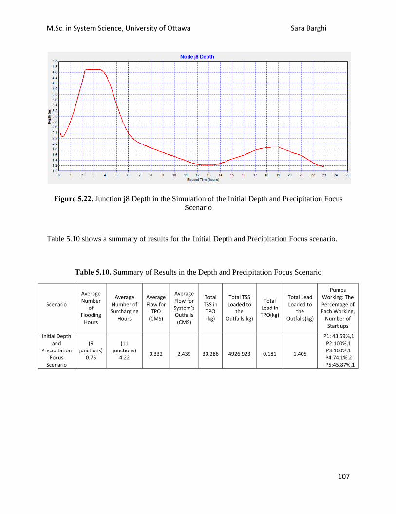
M.Sc. in System Science, University of Ottawa Sara Barghi
107
Figure 5.22. Junction j8 Depth in the Simulation of the Initial Depth and Precipitation Focus Scenario
Table 5.10 shows a summary of results for the Initial Depth and Precipitation Focus scenario.
Table 5.10. Summary of Results in the Depth and Precipitation Focus Scenario
Scenario
Average Number
of Flooding
Hours
Average Number of Surcharging
Hours
Average Flow for
TPO (CMS)
Average Flow for System’s Outfalls (CMS)
Total TSS in TPO (kg)
Total TSS Loaded to
the Outfalls(kg)
Total Lead in TPO(kg)
Total Lead Loaded to
the Outfalls(kg)
Pumps Working: The Percentage of Each Working,
Number of Start ups
Initial Depth and
Precipitation Focus
Scenario
(9 junctions)
0.75
(11
junctions) 4.22
0.332
2.439
30.286
4926.923
0.181
1.405
P1: 43.59%,1 P2:100%,1 P3:100%,1
P4:74.1%,2 P5:45.87%,1

M.Sc. in System Science, University of Ottawa Sara Barghi
108
5.2.10. Initial Depth and Impervious Percentage Focus Scenario Results The Tide and Initial Depth Focus Scenario is presented in section 5.1.10. As before, the
continuity errors for surface runoff, flow routing and quality routing are all acceptable at rates of
-%0.04, -%0.58 and -%0.29, respectively. None of the junctions have a continuity error more
than 10%.
The runoff summary for this scenario is the same as for the Worst Case scenario because of the
same impervious percentage for subcatchments, and the same front loaded precipitation case
(P3) used for both scenarios. The Washoff summary is the same as the Worst Case and
Precipitation Focus scenario because of the same amount of precipitation in the system for these
scenarios.
Junctions’ average depths on the High Road are the same as the depths in the Worst Case
scenario and the Precipitation Focus scenario. The treatment plant average depth is lower than
the Worst Case Scenario. For all the storage units, the average depths are very close to the values
in the Worst Case scenario but higher than values in the Precipitation Focus scenario because of
the initial depth considered for the junctions in the current scenario. The maximum depths for
most junctions are very close to the Worst Case scenario. For the outfalls, because of the
difference in the tidal level the average and maximum depth, flow is higher in the Worst Case
scenario. Outfall flows are very close to the Precipitation Focus values.
Eleven junctions are surcharged and 10 junctions are flooded in this scenario. In comparison
with the Worst Case scenario, the “TreatmentPlant” is surcharged for the same number of hours
but other junctions are surcharged for fewer numbers of hours during the simulation. It seems
that the change in the tidal level time series does not have any impact on the treatment plant
surcharged time due to the same results for the two scenarios. Junction j11 is surcharged for less
than 5 hours and this attributed to j10 being surcharged for less than 3 hours so that less volume
of water is pumped up to j11. The timing for the surcharged junctions is very close to the values
in the Precipitation Focus Scenario, however, junction j14 is not flooded in the Precipitation
Focus scenario as it is here.
For the flooded junctions, the same junctions are flooded as in the Worst Case scenario. All the
junctions are flooded almost the same number of hours as for the Worst Case scenario except for

M.Sc. in System Science, University of Ottawa Sara Barghi
109
j10 which is flooded for 0.14 fewer hours. According to the flooding results and the graph in
Figure 5.22 all the flooding occurs in the first 5 hours of the simulated scenario because of the
high precipitation during this time. In the Precipitation Focus scenario, only 5 junctions are
flooded and the number of hours they are flooded is lower than the same value for the same
junctions in the current scenario. This shows that the higher initial depth and impervious
percentage in the junctions causes more flooding in the system. Comparing Figure 5.11 and
Figure 5.22, the highest values of flooding is proof of the impact of the initial depth and the
impervious percentage on the flooding volume.
Figure 5.23. System Flooding for the Initial Depth and Impervious Focus Scenario
The amount of TSS and Lead which are loaded into the outfalls are close to the Worst Case
scenario and lower than the Precipitation Focus scenario. The pumps are working very
differently in this case compared to the Precipitation Focus scenario and the Worst Case
scenario. The summary results for this scenario are shown in Table 5.11.

M.Sc. in System Science, University of Ottawa Sara Barghi
110
Table 5.11. Summary of Results for the Initial Depth and Impervious Percentage Focus Scenario
Scenario
Average Number of Flooding Hours
Average Number of Surcharging
Hours
Average Flow for
TPO(CMS)
Average Flow for System’s Outfalls (CMS)
Total TSS in TPO (kg)
Total TSS Loaded to
the Outfalls(kg)
Total Lead in TPO(kg)
Total Lead Loaded to
the Outfalls(kg)
Pumps Working: The Percentage of Each Working,
Number of Start ups
Initial Depth and Impervious Percentage
Focus Scenario
(10 junctions) 1.18
(11 junctions)
4.29
0.336
2.618
34.931
4667.476 0.152
1.310
P1: 33.81%,1 P2:100%,1 P3:100%,1
P4:69.46%,2 P5:37.98%,1
5.3 Analysis of the Results Results of the 10 simulation model scenarios are presented above in section 5.2 and provide
rationale for understanding the Arichat water system and the important occurrences discovered
for each of the scenarios. Table 5.12 presents the collected summary of the scenario analysis
results for all 10 scenarios as presented individually in Tables 5.2 through 5.11, respectively.
This consolidated table is presented for comparative purposes and is referred to in the analysis
presented below.

M.Sc. in System Science, University of Ottawa Sara Barghi
111
Table 5.12. Results summary for scenario 1 to 10
Scenario
Average Number of Flooding Hours
Average Number of Surcharging Hours
Average Flow for TPO(CMS)
Average Flow for System’s Outfalls (CMS)
Total TSS in TPO (kg)
Total TSS Loaded to the Outfalls(kg)
Total Lead in TPO(kg)
Total Lead Loaded to the Outfalls(kg)
Pumps Working: The Percentage of Each Working, Number of Start ups
(1) SQ --- ---
0.12
0.388 1.201
56.217 0.015
0.029
P1:0%,0 P2:80.4%, 1 P3:85.29%,1 P4:20.91%,1 P5:0%,0
(2) Best Case
--- --- 0.01
0.01 0.013
0.013 0.01
0.01
P1:0%,0 P2:0%,0 P3:0%,0 P4:0%,0 P5:0%,0
(3) Worst Case
(11 junctions) 1.94
(10 junctions) 6.54
0.405
2.805 36.229
4658.107
TPO:0.151
1.307
P1:84.35%,2 P2:100%,1 P3:100%,1 P4:100%,1 P5:38.82%,1
(4) Precipitation Focus
(5 junctions) 1.23
(10 junctions) 4.293
0.328
2.288 29.909
4909.817 0.179
1.399
P1:39.58%,1 P2:96.45%,1 P3:95.77%,1 P4:70.12%,2 P5:41.89%,1
(5) Tide Focus
---
(10 junctions) 2.47
0.185
0.608 2.534
32.337 0.015
0.022
P1:15.48%,1 P2:96.67%,1 P3:93.15%,1 P4:59.32%,1 P5:0%,0
(6) Tide and Initial Depth Focus
(5 junctions) 0.01
(10 junctions) 5.0525
0.344
1.6
27.476
3773.241
0.272
1.209
P1:100%,1 P2:100%,1 P3:100%,1 P4:100%,1 P5:81.21%,2
(7) Regulators and Precipitation Focus
(9 junctions) 9.226
(12 junctions) 16.19
0.487
0.487
118.214
118.214
0.327
0.327
P1:96.16%,1 P2:96.07%,1 P3:95.18%,1 P4:96.07%,1 P5:96.22%,1
(8) Tide and Impervious Focus
----
(6 junctions) 6.84
0.351
1.634 28.983
4080.723 0.298
1.311
P1:69.38%,1 P2:96.88%,1 P3:94.28%,1 P4:74.24%,1 P5:74.42%,1
(9) Initial Depth and Precipitation Focus
(9 junctions) 0.75
(11 junctions) 4.22
0.332
2.439 0.286
4926.923 0.181
1.405
P1:43.59%,1 P2:100%,1 P3:100%,1 P4:74.1%,2 P5:45.87%,1
(10) Initial Depth & Impervious Percentage Focus
(10 junctions) 1.18
(11 junctions) 4.29
0.336
2.618 34.931
4667.476 0.152
1.310
P1:33.81%,1 P2:100%,1 P3:100%,1 P4:69.46%,2 P5:37.98%,1

M.Sc. in System Science, University of Ottawa Sara Barghi
112
Table 5.13 shows the consolidated flooding summary for junctions flooded in the different
scenarios. Also, it shows the frequency of being flooded for each junction.
Table 5.13. Flooding Summary for Junctions Flooded in Scenario 1 to 10
Scenarios
Junctions
(1) (2) (3) (4) (5) (6) (7) (8) (9) (10) Frequency
j4 - - - - - - 0.67 - - - 1
j6 - - 2.47 1.88 - - 14.34 - 2.05 2.48 5
j7 - - 0.01 - - 0.01 - - 0.01 0.01 4
j8 - - 1.98 1.14 - - 16.53 - 1.29 1.93 5
j9 - - 0.01 - - 0.01 - - 0.01 0.01 4
j10 - - 1.21 - - - 15.75 - - 1.07 3
j11 - - 1.66 0.19 - 0.01 4.41 - 0.19 1.65 6
j12 - - 0.01 - - 0.01 3.55 - 0.01 0.01 5
j13 - - - - - - 10.38 - - - 1
j14 - - 0.01 - - 0.01 - - 0.01 0.01 4
j15 - - 2.09 1.56 - - 12.33 - 1.73 2.14 5
TP - - 2.49 1.38 - - 5.07 - 1.38 2.49 5
It is possible to analyze these flooding junctions based on the possibility of getting flooded
which is concluded based on the frequency of flooding. Table 5.13 shows that j11 has the highest
frequency of flooding in the 10 scenarios. Over the 10 scenarios, j11 is flooded in 6 of the 10
scenarios. Although the average number of hours this junction is flooded is low, because of the
high numbers of occurrence of this junction, j11 is identified as the junction who has priority in
terms of causing water quantity problems for the system. On other hand, j13 has the highest
average number of hours being flooded (Table 5.13). The frequency of flooding occurrence for
this junction is only one time in scenario 7. Therefore it is not a good decision if j13 may be
introduced as a problematic junction since in 9 of 10 scenarios it is not at issue.
The next junctions with a high average number of hours flooded are j6, j8, j12, j15 and the
TreatmentPlant. The frequency of occurrence for these junctions is also high. They are flooded in
5 of the 10 scenarios. Junction j12 was not flooded for a high number of hours; therefore, it is not

M.Sc. in System Science, University of Ottawa Sara Barghi
113
designated as a problem junction for the system. The other 4 junctions can be introduced as
junctions that may cause water quantity problems for the system. Based on personal
communications with the Municipality of Richmond County Public Works engineer in Arichat,
junctions j6 and j8 are more probable to get flooded in heavy storms in comparison with other
junctions. This empirical report validates in part these model findings.
Table 5.14 shows the same values as shown in Table 5.13 for flooded junctions, but this time is
prepared for surcharged junctions. Junctions getting surcharged are not necessarily flooded.
Junction j8 to j13 have the highest frequency and among them, junction j11 has the highest mean
number of hours flooded. Junction j6 has lower frequency with a high mean number of hours
flooded. It seems j11 and j6 are the most problematic junctions in the system. Junction j15 is also
surcharged 5 times with a mean duration of 7.914 which seems to be high in comparison with
other junctions.
Table 5.14. Surcharging Summary for Junctions surcharged in Scenario 1 to 10
Scenarios
Junctions
(1) (2) (3) (4) (5) (6) (7) (8) (9) (10) Frequency
j4 - - - - - - 0.96 - - - 1
j6 - - 5 4.79 - - 21.96 - 5.24 5.01 5
j7 - - 3.09 2.39 - 0.05 21.4 - 2.62 3.05 6
j8 - - 6.24 4.48 1.53 1.63 21.9 1.93 4.96 4.77 8
j9 - - 5.8 3.37 1.97 2.16 21.21 2.42 3.59 4.04 8
j10 - - 7.64 4 3.37 4.28 21.49 3.46 4.33 4.53 8
j11 - - 11.11 8.81 3.28 18.6 8.32 20.62 9.4 6.72 8
j12 - - 16.15 5.38 1.24 10.21 6.57 9.41 5.88 5.11 8
j13 - - 6.25 2.31 3.43 3.44 21.89 3.46 2.36 3.61 8
j14 - - 1.63 - - 0.05 21.51 - 0.05 2.29 5
j15 - - 4.46 4.14 - - 21.94 - 4.55 4.48 5
TP - - 3.51 3.26 - - 5.13 - 3.36 3.52 5
Table 5.15 shows a summary on the percentage of pumps utilized and the number of times they
are started up in each scenario. Pump P1 seems to have poor performance. Based on Table 5.13,

M.Sc. in System Science, University of Ottawa Sara Barghi
114
j15, the inlet of the pump P1, is flooded in scenarios 3, 4, 7, 9 and 10, and mostly for a
significant number of hours. But, as it is shown in Table 5.15, this pump is not working properly
and the utilization percentage is very low for most of the scenarios. Pump P2 is working properly
as j13, ,the inlet of this pump, is flooded only in scenario 7 and pump P2 utilization percentage
for this scenario is close to 100%. Pump P3 also has a good performance. Junction j10 connected
to this pump, is not flooded for a significant number of hours. P3 lifts up water to j11 and, j11
because of insufficient capacity, is flooded. Pumps P4 and P5 are connected to j8 and j6,
respectively. These two junctions are the two junctions with high frequency of flooding and high
average number of hours flooded. P4 and P5 performance seem moderate because the utilization
percentage is almost high for most of the scenarios and for those scenarios that the utilization
percentage is low, the number of hours the connected junctions are flooded is very low.
Table 5.15. Utilization Percentage for Pumps 1 to 5 in the Scenarios 1 to 10
scenarios
Pumps
(1) (2) (3) (4) (5) (6) (7) (8) (9) (10)
P1 0%,0 0%,0 84.35%,1 39.58%,1 15.48%,1 100%,1 96.16%,1 69.38%,1 43.59%,1 33.81%,1 P2 80.49%,1 0%,0 100%,1 96.45%,1 96.67%,1 100%,1 96.07%,1 97.88%,1 100%,1 100%,1 P3 85.29%,1 0%,0 100%,1 95.77%,1 93.15%,1 100%,1 95.18%,1 94.28%,1 100%,1 100%,1 P4 20.91%,1 0%,0 100%,1 70%,2 59.32%,1 100%,1 96.07%,1 74.24%,1 74.1%,2 69.46%,2 P5 0%,0 0%,0 38.82%,1 41.89%,1 0%,0 81.21%,2 96.22%,1 74.42%,2 45.87%,1 37.98%,1

M.Sc. in System Science, University of Ottawa Sara Barghi
115
6. Conclusion, Suggestions and Recommendations for Future Study This chapter has 3 sections: (6.1) Summary of Results, (6.2) Conclusions and Suggestions for
Improvement of the Water System in Arichat, (6.3) Recommendations for Future Study. The first
section of this chapter summarizes the results of this research in terms of the original research
objectives (section 1.2). The second section presents the model conclusions and suggestions for
improvement in the water system infrastructure in Arichat based on the results achieved in this
research. The final section discusses recommendations for future study.
6.1. Summary of Results The thesis research objectives were stated in Chapter 1, Section 1.2. In this section, the following
objectives were present. These are discussed in terms of the thesis results:
1) Model a selected community’s sewage and stormwater systems components using
SWMM. In achieving this objective, the community of Arichat, a coastal community
located on the island of Isle Madame in Cape Breton, N.S is selected as the case study
and SWMM, version 5 is used as the modeling tool in .this research. In Chapter 3,
SWMM capabilities are discussed. Chapter 4 explains how these capabilities are applied
in modeling the Arichat water system. Water system components modeled in SWMM
and the properties for each model component are presented in Chapter 4. This work
accomplishes the stated objective.
2) Acquire data on storms and storm impacts of stormwater on selected coastal
communities. In order to achieve this objective, precipitation and tidal level time series
data were prepared in order to appropriately simulate the water system model in Arichat.
These data are discussed in Chapter 4. Chapter 5 presents the simulation design for the
structured investigation of simulated impacts the water system. A suite of ten (10)
simulation scenarios were developed and defined in Chapter 4 including defining the
status quo scenario. The scenarios were constructed and used to test and validate the
functioning and capacity of the actual system.
3) Evaluate storm impacts using the SWMM stormwater model. This objective is achieved
through the structured analysis and results of the simulation of the water system model
based on the 10 scenarios. The SWMM model was applied to all 10 scenarios using the
data, and the impacts of all these scenarios analyzed and results presented in summary in

M.Sc. in System Science, University of Ottawa Sara Barghi
116
Chapter 5. The detailed results for all 10 scenarios are presented in Appendix B –
Simulation Scenario Model Results. The model results assist in identifying problematic
components in the system and uncovering solutions for problems that a future severe
storm may cause. Chapter 5 discusses the SWMM model scenario by scenario analysis
and compares each to the SQ Benchmark scenario in order to discover the sensitivity and
the robustness of the Arichat water system. The final chapter, Chapter 6 suggests
probable solutions for the problems.
4) Communicate the results to communities and find strategies for managing adaptation in
selected communities. During the research process, this research has presented to
community leaders in personal meetings, and at national and international conferences as
part of the C-Change “community of practice” (Lane et al 2013). Moreover, this thesis
document has been prepared as a report that will be delivered directly to the Public
Works Engineer at the Municipality of the County of Richmond, as well as to other C-
Change project community partners. As noted elsewhere, the Municipality has been an
excellent and most welcome provider of data for this research without whom the detail of
the SWMM model would not have been as precise. Therefore, it is understood that, the
results and discussions of this research are of interest to and will communicated directly
to the Arichat community through this thesis report and pending presentations, etc.
6.2. Conclusions and Suggestions for Improvement of the Water System in Arichat Section 5.3 discusses water system components which cause problems in the Arichat water
system based on the observations of impacts from the simulations of the model in different
scenarios. The following items present the focused summary of issues in the water system and
conclude options for improved flow and performance of the Arichat water system.
6.2.1. Pump P1 Performance Based on the discussion in Chapter 5, there is evidence that pump P1 does not perform
appropriately and it seems its capacity for lifting up water from j15 is not sufficient. The
performance of a pump is evaluated based on its performance curve. The suggestion here is to
improve P1 performance by upgrading its performance curve. This can happen by either

M.Sc. in System Science, University of Ottawa Sara Barghi
117
changing the pumps physical components, or by changing the pump itself with a new pump with
a better characteristic performance curve.
6.2.2. Junction j11 Capacity In addition to the pump with a problem, j11 is the most problematic junction in the system based
on the analysis presented in section 5.3. The problem with this junction is its low surcharge depth
and low maximum depth in comparison with other junctions in the system. Actually, junction j11
has the lowest values for these properties among all other junctions. The suggestion for
improving the capacity of this junction is to change its surcharge depth and maximum depth to a
higher value. It can happen by changing its physical appearance and/or lowering the level of the
storage and manhole station.
6.2.3. Junctions j6 and j8 Capacities Based on the results of section 5.3, junctions j6 and j8 are also junctions which cause problems.
These junctions have also been pointed as problematic in personal communication with the
Arichat Public Works Engineer. These junctions receive water from large areas which cause lots
of inflow into these junctions. As well, the performance of the pumps P4 and P5 are only
moderate performers based on the discussion in section 5.3. Consequently, under storm pressure,
these two pumping stations do not have enough capacity to handle the large amount of water
inflow into the system during a severe precipitation and storm. It is suggested that adding another
station to this area to would reduce the burden on the two other pumping stations. Alternatively,
another suggestion is to improve the performance of the pumps while increasing the capacity of
these two junctions.
6.2.4. Treatment Plant Capacity The ability of the water system to manage current and future more severe storms is limited by
the capacity of the Treatment Plant. Although the treatment plant is able to flow aerate and scrub
sewage water in the system, some untreated water flows out of the system through the Treatment
Plant outfall which is connected to the treatment plant. As noted above, the treatment plant is
flooded in 5 of 10 scenarios simulated, which indicates that the capacity of the treatment plant is

M.Sc. in System Science, University of Ottawa Sara Barghi
118
not enough during the large precipitation and storms events to treat all the water entering the
system, and results in overflows and the release of untreated water into the harbour. The
conclusion and suggestion here is that increasing the treatment plant capacity and improving the
treatment plant facility, e.g., by including more efficient and rigorous aeration, scrubbing
methods, chlorine treatment, and a larger ponded area, in order to result in better overall water
quality..
6.3. Recommendations for Future Study A review of the research leads to recommendations for the future study of this work on coastal
community water systems, especially in light of raising seas, and more frequent and severe storm
surge. These recommendations are discussed below.
6.3.1 Data The first and the most important item that should be considered in the future extension of this
research is data. Each component in the SWMM can have different properties; lack of data for
each component properties was one issue during this research. A recommendation can be finding
more exact data for these components. Considerable estimations used in this research due to lack
of data. For example, precipitation time series and tidal level time series were proxy of Arichat
for this research. Exact data related to the precipitation and tidal values can be searched and
found for Arichat.
6.3.2 Water Quality Water quality is an important issue in the water systems. The data used for estimating water-
borne pollutants and treatment plant effectiveness in this model were taken from examples used
for different contexts in SWMM. In order to achieve real results related to Arichat community, it
is recommended that the actual values related to the treatment plant and pollutants exist in this
community be used for this water system modeling in SWMM.

M.Sc. in System Science, University of Ottawa Sara Barghi
119
6.3.3. Application to Other Coastal Communities This research and modeling work is provided for the ultimate use and application to other coastal
communities’ water system, e.g., Gibsons, British Columbia (as referred to in section 2.3). The
model is made available to other communities, e.g., in the C-Change project, and can be readily
used as a basic guide for a better simulation of their water systems with SWMM.

M.Sc. in System Science, University of Ottawa Sara Barghi
120
7. Bibliography Arnell, N. W. 1999, Climate change and global water resources. Global Environmental Change,
9: 31-49.
Atlantic Flyway Shorebird Business Strategy Planning Team, 2013. Hurricane Sandy: Rapid Assessment, Final report.
Blake, E. S., Kimberlain, T. B., Berg, R. J., Cangialosi, J.P. and Beven, J. L. II, 2013,Tropical Cyclone Report: Hurricane Sandy (AL182012) 22 – 29 October 2012.
Camare, M.H. 2011.Multicriteria decision evaluation of adaptation strategies for vulnerable coastal communities. University of Ottawa, Master of System Science Thesis.
Cambez, M.J., Pinho, J., David, L.M., 2008. Using SWMM 5 in the continuous modelling of stormwater hydraulics and quality, 11th International Conference on Urban Drainage, Edinburgh, Scotland, UK.
Cash.R, C. Donnelly AND A. Valpy, 2008. Canada's Water Problems: The National Water Picture.
Kundzewicz, Z. W., L. J. Mata, N. W. Arnell, P. Doll, P. Kabat, B. Jiménez, K. A. Miller, T. Oki, Z. SenandI AND A. Shiklomanov, 2007. Freshwater resources and their management.ClimateChange 2007: Impacts, Adaptation and Vulnerability. Contribution of Working Group II to the Fourth Assessment Report of the Intergovernmental Panel on Climate Change, M. L. Parry, O. F. Canziani, J. P. Palutikof, P. J. vander Linden AND C. E. Hanson, Eds., Cambridge University Press, Cambridge, UK, 173-210.
Laing, R. D. 2002. The North Battleford water inquiry, on behalf of the Canadian Union of Public Employees. Local 287.
Lane, D.E., Mercer Clarke, C., Forbes, D., and Watson, P. 2013. The Gathering Storm: Managing Adaptation to Environmental Change in Coastal Communities and Small Islands, Special Issue Sustainability Science.
Lane, D. E., and P. Watson. 2010. Managing adaptation to environmental change in coastal communities: Canada and the Caribbean. Submitted to the 11th Annual Conference of the Sir Arthur Lewis Institute of Social and Economic Studies (SALISES), St. Augustine Campus, University of the West Indies, March 24-26, 2010, St. Augustine, Trinidad&Tobago.
Lindgren, R.D.,2003, In the wake of the walkerton tragedy: The top 10 questions,Publication No.440.

M.Sc. in System Science, University of Ottawa Sara Barghi
121
Louisiana Department of Health and Hospitals, 2006, Deceased. Marshall, D., 2002, Final Report:Panel review of British Colombia’s drinking water protection act.
Lowe,S.A.,2010. Sanitary sewer design using EPA storm water management model (SWMM). Computer Applications in Engineering Education, volume 18, 2:203-212.
International Hydrographic Bureau, 2005, Manual on Hydrography:1st Edition, Chapter 5: Water Levels and Flow.
Mimura, N. , L. Nurse, R. F. McLean, J. Agard, L. Briguglio, P. Lefale, R. Payetand AND G.Sem. 2007.Small islands. Climate Change 2007: Impacts, Adaptation and Vulnerability. Contribution of Working Group II to the Fourth Assessment Report of the Intergovernmental panel on Climate change , M.L.Parry ,O.F.Canziani ,J.P.Palutikof, P.J.VanderLindenandC.E.Hanson,Eds.,CambridgeUniversity Press,Cambridge,UK,687-716.
Ministry of Community Services British Columbia, 2006, Improvement Discrete Manual.Ministry of Environment Biritish Colombia,RSBC 1996, Water Act.
Ministry of Environment, Ontario,2010. Policy review of Municipal Stormwater Management in the light of climate change-Summary report.
Ministry of Health Services, British Colombia. 2002. Action plan for safe drinking water in British Columbia.
Moy, P., G. Clark, D. Hart, D. Mickelson, A. Luloff, K. Angle, K. Barret, C. Wu, AND S. Bol ,2010. Climate Change and Wisconsin’s Great Lakes Coastal Communities. Coastal Communities Working Group Report.
Municipality of the County of Richmond, 2011, Municipal Planning Strategy and Land Use By-law for the Isle Madame Planning Area.
Municipality of the County of Richmond, 2003, CBCL Arichat Sewage System Study, Report No.011022.
Pakdel, S., 2011. Spatial–temporal modelling for estimating impacts of storm surge and sea level rise on coastal communities: the case of Isle Madame in cape Breton, Nova Scotia, Canada. University of Ottawa, Master of System Science Thesis.
Park, J., Obeysekera, J., Irizarry, M., Barnes, J., Trimble, P. and Park-Said, W. 2011. Storm surge projections and implications for water management in South Florida. Climate Change, 107:109-128.

M.Sc. in System Science, University of Ottawa Sara Barghi
122
Pollution Probe, 2004.The Source Water Protection Primer Report. ISBN-0-919764-56-8. Prudham, S., 2004, Poisoning the well: neoliberalism and the contamination of municipal water in Walkerton, Ontario, Geoforum, Volume 35:343-359..
Rossman, L. A., 2006.Storm Water Management Model Quality Assurance Report: Dynamic Wave Flow Routing. Environmental Protection Agency of United States of America.
Rossman, L. A., 2010. Stormwater Management Model user's manual version 5.0. Environmental Protection Agency of United States of America.
Simeone,T., 2010. Safe Drinking Water in First Nations Communities. Parlimentary Information and Research Service,Publication No. 08-43-E.
Stephens, K. A., P. Graham AND D. Reid, 2002. Stormwater planning: A guide book for British Colombia.
Tienaah,T. and Rak, A., 2011, RTK Survey to Map Precise Positions:Arichat and Petit-de-Grat, Isle Madamee,Nova Scotia.
Young,K.D., Younos, T.,Daymond, R.L.,Kibler,D.F. AND Lee,D.H.,2010. Application of the analythic hierarchy process for selecting and modeling stormwater best management practices, Contemporary Water Research & Education,146:50-63.
Weblink References:
C-Change-Coastal Climate Adaption Strategies-Canada-Carribean, Accessed 04/03/2012, Copyright 2011, http://www.coastalchange.ca
Climate Institute, Climate Change and Sea Level Rise, Accessed 29/02/2012, Copyright 2007-2010, http://www.climate.org/topics/sea-level/index.html
Environment Canada: Federal Policy & Legislation, Accessed: 08/03/2012, Last updated: 27/01/2012, http://ec.gc.ca/eau-water/default.asp?lang=En&n=E05A7F81-1
Federation of Canadian Municipalities: Wastewater, Accessed: 21/03/2012, Last updated: 20/3/2012, http://www.fcm.ca/home/issues/environment/wastewater.htm
National Climatic Data Center,US Department of Commerce:Hurricane Katrina,Accessed:18/04/2012,Last Updataed:29/12/2005, http://www.ncdc.noaa.gov/special- reports/katrina.html

M.Sc. in System Science, University of Ottawa Sara Barghi
123
Ministry of Environment, Ontario: Stormwater Management, Accessed: 02/04/2012, Last updated: 18/11/2010, http://www.ene.gov.on.ca/environment/en/subject/ stormwater_management/index.htm
Photoshop, Copy right: 2013, http://www.photoshop.com/
Project Blue: Roots and Shoots Canada Water Campaign, Accessed: 14/11/2011, Last updated: 2008, http://www.janegoodall.ca/project-blue
Richmond County: General Description of Sewer Systems, Accessed: 30/3/2013, http://www.richmondcounty.ca/default.asp?mn=1.48.51
The Council of Canadians: Water crisis in Attawapiskat, Accessed: 18/04/2012, Last updated: 30/11/2011, http://canadians.org/blog/?p=12346
Town of Gibsons, The Official Website of Town of Gibsons, British Colombia, Accessed: 3/04/2012, http://www.gibsons.ca
Wikipedia: Attawapiskat First Nation, Accessed, 18/04/2012, Last updated: 26/02/2012, http://en.wikipedia.org/wiki/Attawapiskat_First_Nation
Wikipedia: Fukushima Daiichi nuclear disaster, Accessed: 18/04/2012, Last updated: 18/04/2012, http://en.wikipedia.org/wiki/Fukushima_Daiichi_nuclear_disaster
Yukon Water resources,Accessed 14/11/2011, Last updated 05/03/2011, http://yukonwater.ca
EPA:United States Environmental Agency: Stormwater Manament Modelling(SWMM) ,Accessed 7/01/2013, Last updated:14/12/2012, http://www.epa.gov/nrmrl/wswrd/wq/models/swmm/
Xylect Professional, Accessed: 8/04/2013, http://www.xylect.com
Personal Conversations:
Rossman, L., 2012, via email: [email protected].
Personal Meetings:
Boudreau, C., 2013, Positon: Director of Public Works / Municipal Engineer at Municipality of the County of Richmond, Location: MCCAP workshop, Truro, Nova Scotia.

M.Sc. in System Science, University of Ottawa Sara Barghi
124
Appendix A Precipitation Data Summary
The following histograms contained in this appendix are the maximum and minimum monthly
average precipitation in the precipitation data set (Environment Canada, 2012). For a better view
of the histogram data, please note that the precipitation values between 0 mm and 1 mm are
eliminated from the data.
Figure A.1. Maximum monthly average precipitation histogram excluding 0mm to 1mm precipitation
Figure A.2. Minimum Monthly average precipitation precipitation histogram excluding 0mm to 1mm precipitation
0
10
20
30
40
50
60
70
80
90
1-2 2-3 3-4 4-5 5-6 6-7 7-8 8-9
0
10
20
30
40
50
60
70
80
1-2 2-3 3-4 4-5 5-6 6-7 7-8 8-9 9-10

M.Sc. in System Science, University of Ottawa Sara Barghi
125
Appendix B
SWMM Model Regulator Rules Definitions
The following lines of code are used in the SWMM model to show the “Open” alternative for
regulators in the Arichat water system. The code applies to all six (6) of the regulators in the
system.
RULE R1 IF NODE j6 DEPTH >= 2.591 THEN WEIR R1 SETTING = 1 PRIORITY 1 RULE R2 IF NODE j8 DEPTH >= 2.591 THEN WEIR R2 SETTING = 1 PRIORITY 1 RULE R3 IF NODE j10 DEPTH >= 2.591 THEN WEIR R3 SETTING = 1 PRIORITY 1 RULE R4 IF NODE Treatmentplant DEPTH >= 2.591 THEN WEIR R4 SETTING = 1 PRIORITY 1 RULE R5 IF NODE j13 DEPTH >= 2.591 THEN WEIR R5 SETTING = 1 PRIORITY 1 RULE R6 IF NODE j15 DEPTH >= 2.591 THEN WEIR R6 SETTING = 1 PRIORITY 1

M.Sc. in System Science, University of Ottawa Sara Barghi
126
The following lines show the “Close” alternative for regulators in the Arichat water system
modeling in SWMM. The code applies to all six (6) of the regulators in the system.
RULE R1 IF NODE j6 DEPTH >= 0 THEN WEIR R1 SETTING = 0 PRIORITY 1 RULE R2 IF NODE j8 DEPTH >= 0 THEN WEIR R2 SETTING = 0 PRIORITY 1 RULE R3 IF NODE j10 DEPTH >= 0 THEN WEIR R3 SETTING = 0 PRIORITY 1 RULE R4 IF NODE Treatmentplant DEPTH >= 0 THEN WEIR R4 SETTING = 0 PRIORITY 1 RULE R5 IF NODE j13 DEPTH >= 0 THEN WEIR R5 SETTING = 0 PRIORITY 1 RULE R6 IF NODE j15 DEPTH >= 0 THEN WEIR R6 SETTING = 0 PRIORITY 1

M.Sc. in System Science, University of Ottawa Sara Barghi
127
Appendix C SWMM Model Simulation Scenario Results
The Arichat water system model output status reports for each of the 10 simulation scenarios is provided in this appendix.
NOTE: The summary statistics displayed in these reports are based on results found at every computational time step, not just on results from each reporting time step.
C.1. Status Quo Scenario Simulation Status Report **************** Table C.1. Analysis Options: SQ Scenario
**************** Flow Units............... CMS Process Models: Rainfall/Runoff........ YES Snowmelt............... NO Groundwater............ NO Flow Routing........... YES Ponding Allowed........ YES Water Quality.......... YES Infiltration Method...... HORTON Flow Routing Method...... DYNWAVE Starting Date............ DEC-14-2010 00:00:00 Ending Date.............. DEC-14-2010 23:00:00 Antecedent Dry Days ...... 5.0 Report Time Step ......... 00:05:00 Wet Time Step ............ 00:05:01 Dry Time Step ............ 00:05:01 Routing Time Step........ 30.00 sec ************************** Table C.2. Runoff Quantity Continuity: SQ Scenario
************************** Volume Depth Hectare-m mm --------- ------- Total Precipitation ...... 1.381 6.925 Evaporation Loss ......... 0.000 0.000 Infiltration Loss........ 0.924 4.636 Surface Runoff........... 0.413 2.071 Final Surface Storage.... 0.044 0.222 Continuity Error (%)..... -0.060

M.Sc. in System Science, University of Ottawa Sara Barghi
128
************************** Table C.3. Runoff Quality Continuity: SQ Scenario
************************** TSS Lead kg kg ---------- ---------- Initial Buildup .......... 6111.392 0.000 Surface Buildup .......... 1.777 0.048 Wet Deposition........... 0.000 0.000 Sweeping Removal ......... 0.000 0.000 Infiltration Loss........ 0.000 0.000 BMP Removal.............. 0.000 0.000 Surface Runoff........... 193.201 0.048 Remaining Buildup........ 5919.581 0.000 Continuity Error (%)..... 0.006 0.000 ************************** Table C.4. Flow Routing Continuity: SQ Scenario
************************** Volume Volume Hectare-m 10^6 ltr ----------- --------- Dry Weather Inflow ....... 0.000 0.000 Wet Weather Inflow ....... 0.410 4.104 Groundwater Inflow ....... 0.000 0.000 RDII Inflow.............. 0.000 0.000 External Inflow .......... 1.727 17.265 External Outflow ......... 1.476 14.756 Internal Outflow ......... 0.000 0.000 Storage Losses........... 0.000 0.000 Initial Stored Volume.... 0.000 0.000 Final Stored Volume ...... 0.627 6.271 Continuity Error (%)..... 1.600
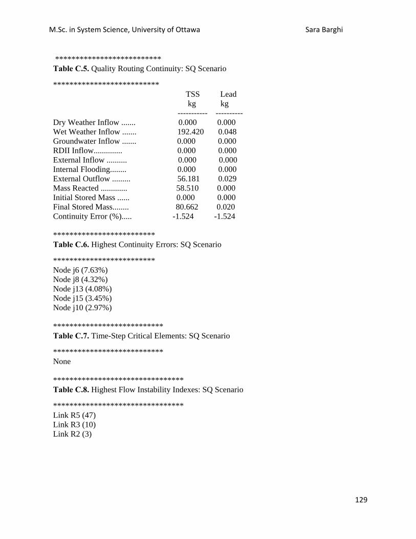
M.Sc. in System Science, University of Ottawa Sara Barghi
129
************************** Table C.5. Quality Routing Continuity: SQ Scenario
************************** TSS Lead kg kg ----------- ---------- Dry Weather Inflow ....... 0.000 0.000 Wet Weather Inflow ....... 192.420 0.048 Groundwater Inflow ....... 0.000 0.000 RDII Inflow.............. 0.000 0.000 External Inflow .......... 0.000 0.000 Internal Flooding........ 0.000 0.000 External Outflow ......... 56.181 0.029 Mass Reacted ............. 58.510 0.000 Initial Stored Mass ...... 0.000 0.000 Final Stored Mass........ 80.662 0.020 Continuity Error (%)..... -1.524 -1.524 ************************* Table C.6. Highest Continuity Errors: SQ Scenario
************************* Node j6 (7.63%) Node j8 (4.32%) Node j13 (4.08%) Node j15 (3.45%) Node j10 (2.97%) *************************** Table C.7. Time-Step Critical Elements: SQ Scenario
*************************** None ******************************** Table C.8. Highest Flow Instability Indexes: SQ Scenario
******************************** Link R5 (47) Link R3 (10) Link R2 (3)

M.Sc. in System Science, University of Ottawa Sara Barghi
130
************************* Table C.9. Routing Time Step Summary: SQ Scenario
************************* Minimum Time Step : 30.00 sec Average Time Step : 29.99 sec Maximum Time Step : 30.00 sec Percent in Steady State : 0.00 Average Iterations per Step : 2.00 *************************** Table C.10. Subcatchment Runoff Summary: SQ Scenario
*************************** -------------------------------------------------------------------------------------------------------- Total Total Total Total Total Total Peak Runoff Precip Runon Evap Infil Runoff Runoff Runoff Coeff Subcatchmen mm mm mm mm mm 10^6 ltr CMS -------------------------------------------------------------------------------------------------------- S1 6.93 0.00 0.00 5.19 1.56 0.41 0.01 0.225 S2 6.93 0.00 0.00 5.19 1.58 0.35 0.00 0.227 S13 6.93 0.00 0.00 3.46 2.99 0.67 0.01 0.432 S11 6.93 0.00 0.00 3.46 3.28 0.14 0.00 0.474 S10 6.93 0.00 0.00 3.46 3.28 0.15 0.00 0.473 S9 6.93 0.00 0.00 3.46 3.19 0.29 0.00 0.460 S8 6.93 0.00 0.00 3.46 3.17 0.31 0.00 0.458 S7 6.93 0.00 0.00 3.46 3.10 0.45 0.01 0.447 S6 6.93 0.00 0.00 5.19 1.64 0.14 0.00 0.237 S3 6.93 0.00 0.00 5.19 1.57 0.39 0.01 0.226 S4 6.93 0.00 0.00 5.19 1.55 0.44 0.01 0.224 S5 6.93 0.00 0.00 5.19 1.61 0.23 0.00 0.233 S12 6.93 0.00 0.00 5.19 1.63 0.18 0.00 0.235
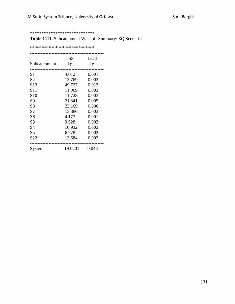
M.Sc. in System Science, University of Ottawa Sara Barghi
131
**************************** Table C.11. Subcatchment Washoff Summary: SQ Scenario
**************************** ------------------------------------------------ TSS Lead Subcatchment kg kg ------------------------------------------------ S1 4.012 0.001 S2 13.769 0.003 S13 49.727 0.012 S11 11.069 0.003 S10 11.728 0.003 S9 21.341 0.005 S8 23.169 0.006 S7 13.386 0.003 S6 4.177 0.001 S3 9.528 0.002 S4 10.932 0.003 S5 6.778 0.002 S12 13.584 0.003 ------------------------------------------------ System 193.201 0.048

M.Sc. in System Science, University of Ottawa Sara Barghi
132
****************** Table C.12. Node Depth Summary: SQ Scenario
****************** ------------------------------------------------------------------------------------------------------------- Average Maximum Maximum Time of Max Depth Depth HGL Occurrence Node Type Meters Meters Meters days hr:min -------------------------------------------------------------------------------------------------------------- j2 JUNCTION 0.02 0.02 17.70 0 23:00 j4 JUNCTION 0.02 0.02 20.13 0 23:00 j1 JUNCTION 0.02 0.02 22.58 0 23:00 j5 JUNCTION 0.01 0.01 21.96 0 23:00 j16 JUNCTION 0.01 0.01 23.01 0 22:29 j3 JUNCTION 0.02 0.02 16.17 0 23:00 Treatmentplant JUNCTION 0.44 0.69 0.70 0 19:01 j11 JUNCTION 0.15 0.17 1.81 0 04:26 j9 JUNCTION 0.03 0.13 2.52 0 19:33 j7 JUNCTION 0.00 0.00 3.59 0 00:00 j12 JUNCTION 0.12 0.15 2.21 0 06:46 j14 JUNCTION 0.00 0.00 2.43 0 00:00 TreatmentPlantOutfall OUTFALL 0.22 0.31 0.31 0 19:01 Outfall4 OUTFALL 0.87 1.33 1.33 0 19:00 Outfall6 OUTFALL 1.10 1.56 1.33 0 19:00 Outfall1 OUTFALL 0.51 0.97 1.33 0 19:00 Outfall2 OUTFALL 1.42 1.88 1.33 0 19:00 Outfall3 OUTFALL 1.79 2.25 1.33 0 19:00 Outfall5 OUTFALL 1.80 2.26 1.33 0 19:00 j6 STORAGE 0.49 0.96 1.32 0 19:04 j8 STORAGE 1.31 1.88 1.33 0 19:00 j10 STORAGE 1.69 2.25 1.33 0 19:00 j13 STORAGE 1.78 2.26 1.33 0 19:00 j15 STORAGE 1.00 1.56 1.33 0 19:00

M.Sc. in System Science, University of Ottawa Sara Barghi
133
******************** Table C.13. Node Inflow Summary: SQ Scenario
******************* ------------------------------------------------------------------------------------------------------------------- Maximum Maximum Lateral Total Lateral Total Time of Max Inflow Inflow Inflow Inflow Occurrence Volume Volume Node Type CMS CMS days hr:min 10^6 ltr 10^6 ltr ------------------------------------------------------------------------------------------------------------------- j2 JUNCTION 0.005 0.006 0 23:00 0.346 0.418 j4 JUNCTION 0.006 0.006 0 23:00 0.440 0.458 j1 JUNCTION 0.005 0.005 0 23:00 0.403 0.403 j5 JUNCTION 0.003 0.003 0 23:00 0.226 0.226 j16 JUNCTION 0.002 0.002 0 22:59 0.139 0.139 j3 JUNCTION 0.005 0.006 0 23:00 0.383 0.455 Treatmentplant JUNCTION 0.006 0.206 0 19:00 0.430 10.013 j11 JUNCTION 0.000 0.043 0 03:23 0.000 3.064 j9 JUNCTION 0.000 0.029 0 17:40 0.000 0.504 j7 JUNCTION 0.000 0.000 0 00:00 0.000 0.000 j12 JUNCTION 0.000 0.031 0 04:31 0.000 2.050 j14 JUNCTION 0.000 0.000 0 00:00 0.000 0.000 TreatmentPlantOutfall OUTFALL 0.000 0.206 0 19:01 0.000 9.930 Outfall4 OUTFALL 0.000 0.121 0 19:00 0.000 4.080 Outfall6 OUTFALL 0.000 0.102 0 05:00 0.000 3.320 Outfall1 OUTFALL 0.000 0.034 0 18:00 0.000 1.423 Outfall2 OUTFALL 0.000 0.118 0 05:00 0.000 3.681 Outfall3 OUTFALL 0.000 0.145 0 02:51 0.000 5.132 Outfall5 OUTFALL 0.000 0.504 0 00:00 0.000 4.455 j6 STORAGE 0.006 0.045 0 18:00 0.446 1.512 j8 STORAGE 0.004 0.126 0 05:00 0.308 3.092 j10 STORAGE 0.000 0.150 0 02:52 0.000 5.395 j13 STORAGE 0.004 0.504 0 00:00 0.320 4.348 j15 STORAGE 0.009 0.111 0 05:00 0.663 2.600 ********************** Table C.14. Node Surcharge Summary: SQ Scenario
********************** No nodes were surcharged. ********************* Table C.15. Node Flooding Summary: SQ Scenario
********************* No nodes were flooded.

M.Sc. in System Science, University of Ottawa Sara Barghi
134
********************** Table C.16. Storage Volume Summary: SQ Scenario
********************** ---------------------------------------------------------------------------------------------------------- Average Avg E&I Maximum Max Time of Max Maximum Volume Pcnt Pcnt Volume Pcnt Occurrence Outflow Storage Unit 1000 m3 Full Loss 1000 m3 Full days hr:min CMS ---------------------------------------------------------------------------------------------------------- j6 0.490 10 0 0.961 20 0 19:04 0.034 j8 1.309 28 0 1.876 40 0 19:00 0.091 j10 1.686 39 0 2.247 52 0 19:00 0.124 j13 1.777 36 0 2.257 46 0 19:00 0.105 j15 0.996 22 0 1.557 35 0 19:00 0.063 *********************** Table C.17. Outfall Loading Summary: SQ Scenario
*********************** --------------------------------------------------------------------------------------------------- Flow Avg. Max. Total Total Total Freq. Flow Flow Volume TSS Lead Outfall Node Pcnt. CMS CMS 10^6 ltr kg kg ---------------------------------------------------------------------------------------------------- TreatmentPlantOutfall 99.71 0.120 0.206 9.930 1.201 0.015 Outfall4 100.00 0.049 0.121 4.080 0.000 0.000 Outfall6 100.00 0.040 0.102 3.320 27.706 0.007 Outfall1 97.65 0.018 0.034 1.423 7.202 0.002 Outfall2 100.00 0.044 0.118 3.681 12.870 0.003 Outfall3 100.00 0.062 0.145 5.132 2.748 0.001 Outfall5 99.96 0.054 0.504 4.455 4.489 0.001 ----------------------------------------------------------------------------------------------------- System 99.62 0.388 0.704 32.021 56.217 0.029

M.Sc. in System Science, University of Ottawa Sara Barghi
135
******************** Table C.18. Link Flow Summary: SQ Scenario
******************** --------------------------------------------------------------------------------------------------------- Maximum Time of Max Maximum Max/ Max/ |Flow| Occurrence |Veloc| Full Full Link Type CMS days hr:min m/sec Flow Depth ---------------------------------------------------------------------------------------------------------- c1 CONDUIT 0.001 0 23:00 0.65 0.04 0.14 c6 CONDUIT 0.006 0 23:00 0.09 0.00 0.50 c9 CONDUIT 0.004 0 23:00 1.11 0.00 0.52 c16 CONDUIT 0.206 0 19:01 1.21 5.71 0.81 c5 CONDUIT 0.003 0 23:00 0.01 0.00 0.51 c11 CONDUIT 0.029 0 19:33 0.71 0.52 0.76 c13 CONDUIT 0.031 0 06:46 0.70 0.69 0.80 c14 CONDUIT 0.000 0 00:00 0.00 0.00 0.50 c2 CONDUIT 0.000 0 23:00 0.22 0.03 0.13 c4 CONDUIT 0.000 0 23:00 0.21 0.02 0.12 c8 CONDUIT 0.005 0 23:00 0.03 0.00 0.51 c10 CONDUIT 0.000 0 00:00 0.00 0.00 0.50 c15 CONDUIT 0.002 0 20:36 0.08 0.00 0.51 c12 CONDUIT 0.043 0 04:26 0.95 0.82 0.84 c3 CONDUIT 0.001 0 23:00 0.44 0.04 0.14 c7 CONDUIT 0.006 0 23:00 0.03 0.00 0.51 P2 PUMP 0.031 0 04:31 1.00 p3 PUMP 0.043 0 03:23 1.00 P5 PUMP 0.000 0 00:00 0.00 P1 PUMP 0.000 0 00:00 0.00 P4 PUMP 0.029 0 17:40 1.00 R4 WEIR 0.121 0 19:00 0.51 R6 WEIR 0.102 0 05:00 0.60 R1 WEIR 0.034 0 18:00 0.37 R2 WEIR 0.118 0 05:00 0.72 R3 WEIR 0.145 0 02:51 0.87 R5 WEIR 0.504 0 00:00 0.87

M.Sc. in System Science, University of Ottawa Sara Barghi
136
*************************** Table C.19. Flow Classification Summary: SQ Scenario
*************************** ----------------------------------------------------------------------------------------------------------- Adjusted --------Fraction of Time in Flow Class -------- Avg. Avg. /Actual Up Down Sub Sup Up Down Froude Flow Conduit Length Dry Dry Dry Crit Crit Crit Crit Number Change ------------------------------------------------------------------------------------------------------------ c1 1.00 0.00 0.00 0.00 0.01 0.99 0.00 0.00 1.69 0.0000 c6 1.00 0.00 0.00 0.00 1.00 0.00 0.00 0.00 0.04 0.0000 c9 1.00 0.00 0.00 0.00 0.87 0.13 0.00 0.00 0.44 0.0000 c1 1.00 0.00 0.00 0.00 1.00 0.00 0.00 0.00 0.48 0.0043 c5 1.00 0.00 0.00 0.00 1.00 0.00 0.00 0.00 0.01 0.0000 c1 1.00 0.00 0.77 0.00 0.23 0.00 0.00 0.00 0.11 0.0004 c13 1.00 0.00 0.20 0.00 0.80 0.00 0.00 0.00 0.39 0.0002 c14 1.00 0.00 1.00 0.00 0.00 0.00 0.00 0.00 0.00 0.0000 c2 1.00 0.00 0.00 0.00 1.00 0.00 0.00 0.00 0.60 0.0000 c4 1.00 0.00 0.00 0.00 1.00 0.00 0.00 0.00 0.59 0.0000 c8 1.00 0.00 0.00 0.00 1.00 0.00 0.00 0.00 0.02 0.0000 c10 1.00 0.00 1.00 0.00 0.00 0.00 0.00 0.00 0.00 0.0000 c15 1.00 0.00 0.00 0.00 1.00 0.00 0.00 0.00 0.02 0.0000 c12 1.00 0.00 0.15 0.00 0.85 0.00 0.00 0.00 0.52 0.0003 c3 1.00 0.00 0.00 0.00 0.04 0.96 0.00 0.00 1.14 0.0000 c7 1.00 0.00 0.00 0.00 1.00 0.00 0.00 0.00 0.02 0.0000 ************************* Table C.20. Conduit Surcharge Summary: SQ Scenario
************************* -------------------------------------------------------------------------------------------- Hours Hours --------- Hours Full -------- Above Full Capacity Conduit Both Ends Upstream Dnstream Normal Flow Limited -------------------------------------------------------------------------------------------- c16 0.01 0.01 0.01 19.57 0.01

M.Sc. in System Science, University of Ottawa Sara Barghi
137
*************** Table C.21. Pumping Summary: SQ Scenario
*************** ------------------------------------------------------------------------------------------------------------------ Min Avg Max Total Power % Time Off Percent Number of Flow Flow Flow Volume Usage Pump Curve Pump Utilized Start-Ups CMS CMS CMS 10^6 ltr Kw-hr Low High ------------------------------------------------------------------------------------------------------------------- P2 80.40 1 0.00 0.03 0.03 2.050 7.07 0.0 100.0 p3 85.29 1 0.00 0.04 0.04 3.065 7.40 0.0 100.0 P5 0.00 0 0.00 0.00 0.00 0.000 0.00 0.0 0.0 P 0.00 0 0.00 0.00 0.00 0.000 0.00 0.0 0.0 P4 20.91 1 0.00 0.03 0.03 0.504 1.93 0.0 100.0 Analysis begun on: Tue Apr 23 17:35:51 2013 Analysis ended on: Tue Apr 23 17:35:51 2013 Total elapsed time: < 1 sec
C.2. Best Case Scenario Simulation Status Report **************** Table C.22. Analysis Options: Best Case Scenario
**************** Flow Units ............... CMS Process Models: Rainfall/Runoff ........ YES Snowmelt ............... NO Groundwater ............ NO Flow Routing ........... YES Ponding Allowed ........ YES Water Quality .......... YES Infiltration Method ...... HORTON Flow Routing Method ...... DYNWAVE Starting Date ............ DEC-14-2010 00:00:00 Ending Date .............. DEC-14-2010 23:00:00 Antecedent Dry Days ...... 5.0 Report Time Step ......... 00:05:00 Wet Time Step ............ 00:05:01 Dry Time Step ............ 00:05:01 Routing Time Step ........ 30.00 sec

M.Sc. in System Science, University of Ottawa Sara Barghi
138
************************** Table C.23. Runoff Quantity Continuity: Best Case Scenario
************************** Volume Depth hectare-m mm ------------ ---------- Total Precipitation ...... 1.381 6.925 Evaporation Loss ......... 0.000 0.000 Infiltration Loss ........ 0.924 4.636 Surface Runoff ........... 0.413 2.071 Final Surface Storage .... 0.044 0.222 Continuity Error (%) ..... -0.060 ************************** Table C.24. Runoff Quality Continuity: Best Case Scenario
************************** TSS Lead kg kg ---------- ---------- Initial Buildup .......... 6111.392 0.000 Surface Buildup .......... 1.777 0.048 Wet Deposition ........... 0.000 0.000 Sweeping Removal ....... 0.000 0.000 Infiltration Loss ........ 0.000 0.000 BMP Removal .............. 0.000 0.000 Surface Runoff ........... 193.201 0.048 Remaining Buildup ........ 5919.581 0.000 Continuity Error (%) ..... 0.006 0.000

M.Sc. in System Science, University of Ottawa Sara Barghi
139
************************** Table C.25. Flow Routing Continuity: Best Case Scenario
************************** Volume Volume hectare-m 10^6 ltr --------- --------- Dry Weather Inflow ....... 0.000 0.000 Wet Weather Inflow ....... 0.410 4.104 Groundwater Inflow ....... 0.000 0.000 RDII Inflow .............. 0.000 0.000 External Inflow .......... 0.000 0.000 External Outflow ........ 0.081 0.811 Internal Outflow ......... 0.000 0.000 Storage Losses ........... 0.000 0.000 Initial Stored Volume .... 0.000 0.000 Final Stored Volume ...... 0.325 3.252 Continuity Error (%) ..... 0.998 ************************** Table C.26. Quality Routing Continuity: Best Case Scenario
************************** TSS Lead kg kg ---------- ---------- Dry Weather Inflow ....... 0.000 0.000 Wet Weather Inflow ....... 192.420 0.048 Groundwater Inflow ....... 0.000 0.000 RDII Inflow .............. 0.000 0.000 External Inflow .......... 0.000 0.000 Internal Flooding ........ 0.000 0.000 External Outflow ......... 0.013 0.010 Mass Reacted ............. 41.678 0.000 Initial Stored Mass ...... 0.000 0.000 Final Stored Mass ........ 140.133 0.035 Continuity Error (%) ..... 5.506 5.506 ************************* Table C.27. Highest Continuity Errors: Best Case Scenario
************************* Node j6 (14.08%) Node j13 (11.06%) Node j8 (10.70%) Node j10 (9.69%) Node j15 (8.59%)

M.Sc. in System Science, University of Ottawa Sara Barghi
140
*************************** Table C.28. Time-Step Critical Elements: Best Case Scenario
*************************** None ******************************** Table C.29. Highest Flow Instability Indexes: Best Case Scenario
******************************** All links are stable. ************************* Table C.30. Routing Time Step Summary: Best Case Scenario
************************* Minimum Time Step : 30.00 sec Average Time Step : 29.99 sec Maximum Time Step : 30.00 sec Percent in Steady State : 0.00 Average Iterations per Step : 2.00 *************************** Table C.31. Subcatchment Runoff Summary: Best Case Scenario
*************************** ------------------------------------------------------------------------------------------------------------------- Total Total Total Total Total Total Peak Runoff Precip Runon Evap Infil Runoff Runoff Runoff Coeff Subcatchmt mm mm mm mm mm 10^6 ltr CMS ------------------------------------------------------------------------------------------------------------------- S1 6.93 0.00 0.00 5.19 1.56 0.41 0.01 0.225 S2 6.93 0.00 0.00 5.19 1.58 0.35 0.00 0.227 S13 6.93 0.00 0.00 3.46 2.99 0.67 0.01 0.432 S11 6.93 0.00 0.00 3.46 3.28 0.14 0.00 0.474 S10 6.93 0.00 0.00 3.46 3.28 0.15 0.00 0.473 S9 6.93 0.00 0.00 3.46 3.19 0.29 0.00 0.460 S8 6.93 0.00 0.00 3.46 3.17 0.31 0.00 0.458 S7 6.93 0.00 0.00 3.46 3.10 0.45 0.01 0.447 S6 6.93 0.00 0.00 5.19 1.64 0.14 0.00 0.237 S3 6.93 0.00 0.00 5.19 1.57 0.39 0.01 0.226 S4 6.93 0.00 0.00 5.19 1.55 0.44 0.01 0.224 S5 6.93 0.00 0.00 5.19 1.61 0.23 0.00 0.233 S12 6.93 0.00 0.00 5.19 1.63 0.18 0.00 0.235

M.Sc. in System Science, University of Ottawa Sara Barghi
141
***************************** Table C.32. Subcatchment Washoff Summary: Best Case Scenario
**************************** ------------------------------------------------ TSS Lead Subcatchment kg kg ------------------------------------------------ S1 4.012 0.001 S2 13.769 0.003 S13 49.727 0.012 S11 11.069 0.003 S10 11.728 0.003 S9 21.341 0.005 S8 23.169 0.006 S7 13.386 0.003 S6 4.177 0.001 S3 9.528 0.002 S4 10.932 0.003 S5 6.778 0.002 S12 13.584 0.003 ------------------------------------------------ System 193.201 0.048

M.Sc. in System Science, University of Ottawa Sara Barghi
142
****************** Table C.33. Node Depth Summary: Best Case Scenario
****************** ------------------------------------------------------------------------------------------------------------------- Average Maximum Maximum Time of Max Depth Depth HGL Occurrence Node Type Meters Meters Meters days hr:min ------------------------------------------------------------------------------------------------------------------- j2 JUNCTION 0.02 0.02 17.70 0 23:00 j4 JUNCTION 0.02 0.02 20.13 0 23:00 j1 JUNCTION 0.02 0.02 22.58 0 23:00 j5 JUNCTION 0.01 0.01 21.96 0 23:00 j16 JUNCTION 0.01 0.01 23.01 0 22:29 j3 JUNCTION 0.02 0.02 16.17 0 23:00 Treatmentplant JUNCTION 0.14 0.15 0.16 0 23:00 j11 JUNCTION 0.00 0.00 1.64 0 00:00 j9 JUNCTION 0.00 0.00 2.39 0 00:00 j7 JUNCTION 0.00 0.00 3.59 0 00:00 j12 JUNCTION 0.00 0.00 2.06 0 00:00 j14 JUNCTION 0.00 0.00 2.43 0 00:00 TreatmentPlantOutfall OUTFALL 0.06 0.07 0.07 0 23:00 Outfall4 OUTFALL 0.56 1.17 1.17 0 10:00 Outfall6 OUTFALL 0.76 1.40 1.17 0 10:00 Outfall1 OUTFALL 0.29 0.81 1.17 0 10:00 Outfall2 OUTFALL 1.08 1.72 1.17 0 10:00 Outfall3 OUTFALL 1.45 2.09 1.17 0 10:00 Outfall5 OUTFALL 1.46 2.10 1.17 0 10:00 j6 STORAGE 0.30 0.67 1.03 0 23:00 j8 STORAGE 0.29 0.63 0.08 0 23:00 j10 STORAGE 0.19 0.41 -0.51 0 23:00 j13 STORAGE 0.22 0.47 -0.46 0 23:00 j15 STORAGE 0.33 0.73 0.50 0 23:00

M.Sc. in System Science, University of Ottawa Sara Barghi
143
******************* Table C.34. Node Inflow Summary: Best Case Scenario
******************* ------------------------------------------------------------------------------------------------------------------- Maximum Maximum Lateral Total Lateral Total Time of Max Inflow Inflow Inflow Inflow Occurrence Volume Volume Node Type CMS CMS days hr:min 10^6 ltr 10^6 ltr ------------------------------------------------------------------------------------------------------------------- j2 JUNCTION 0.005 0.006 0 23:00 0.346 0.418 j4 JUNCTION 0.006 0.006 0 23:00 0.440 0.458 j1 JUNCTION 0.005 0.005 0 23:00 0.403 0.403 j5 JUNCTION 0.003 0.003 0 23:00 0.226 0.226 j16 JUNCTION 0.002 0.002 0 22:59 0.139 0.139 j3 JUNCTION 0.005 0.006 0 23:00 0.383 0.455 Treatmentplant JUNCTION 0.006 0.011 0 23:00 0.430 0.838 j11 JUNCTION 0.000 0.000 0 00:00 0.000 0.000 j9 JUNCTION 0.000 0.000 0 00:00 0.000 0.000 j7 JUNCTION 0.000 0.000 0 00:00 0.000 0.000 j12 JUNCTION 0.000 0.000 0 00:00 0.000 0.000 j14 JUNCTION 0.000 0.000 0 00:00 0.000 0.000 TreatmentPlantOutfall OUTFALL 0.000 0.011 0 23:00 0.000 0.811 Outfall4 OUTFALL 0.000 0.000 0 00:00 0.000 0.000 Outfall6 OUTFALL 0.000 0.000 0 00:00 0.000 0.000 Outfall1 OUTFALL 0.000 0.000 0 00:00 0.000 0.000 Outfall2 OUTFALL 0.000 0.000 0 00:00 0.000 0.000 Outfall3 OUTFALL 0.000 0.000 0 00:00 0.000 0.000 Outfall5 OUTFALL 0.000 0.000 0 00:00 0.000 0.000 j6 STORAGE 0.006 0.010 0 23:00 0.446 0.776 j8 STORAGE 0.004 0.009 0 23:00 0.308 0.702 j10 STORAGE 0.000 0.006 0 23:00 0.000 0.454 j13 STORAGE 0.004 0.007 0 23:00 0.320 0.527 j15 STORAGE 0.009 0.011 0 23:00 0.663 0.802 ********************** Table C.35. Node Surcharge Summary: Best Case Scenario
********************** No nodes were surcharged. ********************* Table C.36. Node Flooding Summary: Best Case Scenario
********************* No nodes were flooded.

M.Sc. in System Science, University of Ottawa Sara Barghi
144
********************** Table C.37. Storage Volume Summary: Best Case Scenario
********************** ------------------------------------------------------------------------------------------------------------------- Average Avg E&I Maximum Max Time of Max Maximum Volume Pcnt Pcnt Volume Pcnt Occurrence Outflow Storage Unit 1000 m3 Full Loss 1000 m3 Full days hr:min CMS ------------------------------------------------------------------------------------------------------------------- j6 0.304 6 0 0.667 14 0 23:00 0.000 j8 0.287 6 0 0.627 13 0 23:00 0.000 j10 0.186 4 0 0.410 9 0 23:00 0.000 j13 0.221 5 0 0.469 10 0 23:00 0.000 j15 0.326 7 0 0.733 16 0 23:00 0.000 *********************** Table C.38. Outfall Loading Summary: Best Case Scenario
*********************** ------------------------------------------------------------------------------------------------------------------- Flow Avg. Max. Total Total Total Freq. Flow Flow Volume TSS Lead Outfall Node Pcnt. CMS CMS 10^6 ltr kg kg ------------------------------------------------------------------------------------------------------------------- TreatmentPlantOutfall 97.07 0.010 0.011 0.811 0.013 0.010 Outfall4 0.00 0.000 0.000 0.000 0.000 0.000 Outfall6 0.00 0.000 0.000 0.000 0.000 0.000 Outfall1 0.00 0.000 0.000 0.000 0.000 0.000 Outfall2 0.00 0.000 0.000 0.000 0.000 0.000 Outfall3 0.00 0.000 0.000 0.000 0.000 0.000 Outfall5 0.00 0.000 0.000 0.000 0.000 0.000 ------------------------------------------------------------------------------------------------------------------- System 13.87 0.010 0.011 0.811 0.013 0.010

M.Sc. in System Science, University of Ottawa Sara Barghi
145
******************** Table C.39. Link Flow Summary: Best Case Scenario
******************** ------------------------------------------------------------------------------------------------------------------- Maximum Time of Max Maximum Max/ Max/ |Flow| Occurrence |Veloc| Full Full Link Type CMS days hr:min m/sec Flow Depth ------------------------------------------------------------------------------------------------------------------- c1 CONDUIT 0.001 0 23:00 0.65 0.04 0.14 c6 CONDUIT 0.006 0 23:00 0.28 0.00 0.12 c9 CONDUIT 0.004 0 23:00 1.13 0.00 0.48 c16 CONDUIT 0.011 0 23:00 0.34 0.31 0.22 c5 CONDUIT 0.003 0 23:00 1.39 0.00 0.34 c11 CONDUIT 0.000 0 00:00 0.00 0.00 0.50 c13 CONDUIT 0.000 0 00:00 0.00 0.00 0.30 c14 CONDUIT 0.000 0 00:00 0.00 0.00 0.50 c2 CONDUIT 0.000 0 23:00 0.22 0.03 0.13 c4 CONDUIT 0.000 0 23:00 0.21 0.02 0.12 c8 CONDUIT 0.005 0 23:00 1.71 0.00 0.45 c10 CONDUIT 0.000 0 00:00 0.00 0.00 0.50 c15 CONDUIT 0.002 0 20:35 1.29 0.00 0.51 c12 CONDUIT 0.000 0 00:00 0.00 0.00 0.30 c3 CONDUIT 0.001 0 23:00 0.44 0.04 0.14 c7 CONDUIT 0.006 0 23:00 2.07 0.00 0.30 P2 PUMP 0.000 0 00:00 0.00 p3 PUMP 0.000 0 00:00 0.00 P5 PUMP 0.000 0 00:00 0.00 P1 PUMP 0.000 0 00:00 0.00 P4 PUMP 0.000 0 00:00 0.00 R4 WEIR 0.000 0 00:00 0.00 R6 WEIR 0.000 0 00:00 0.00 R1 WEIR 0.000 0 00:00 0.00 R2 WEIR 0.000 0 00:00 0.00 R3 WEIR 0.000 0 00:00 0.00 R5 WEIR 0.000 0 00:00 0.00

M.Sc. in System Science, University of Ottawa Sara Barghi
146
*************************** Table C.40. Flow Classification Summary: Best Case Scenario
*************************** ------------------------------------------------------------------------------------------------------------------- Adjusted ------- Fraction of Time in Flow Class ------- Avg. Avg. /Actual Up Down Sub Sup Up Down Froude Flow Conduit Length Dry Dry Dry Crit Crit Crit Crit Number Change ------------------------------------------------------------------------------------------------------------------- c1 1.00 0.00 0.00 0.00 0.01 0.99 0.00 0.00 1.68 0.0000 c6 1.00 0.00 0.00 0.00 0.98 0.02 0.00 0.00 0.29 0.0000 c9 1.00 0.00 0.00 0.00 0.85 0.15 0.00 0.00 0.52 0.0000 c16 1.00 0.00 0.00 0.00 1.00 0.00 0.00 0.00 0.37 0.0001 c5 1.00 0.00 0.00 0.00 0.86 0.14 0.00 0.00 0.60 0.0000 c11 1.00 0.01 0.99 0.00 0.00 0.00 0.00 0.00 0.00 0.0000 c13 1.00 0.00 1.00 0.00 0.00 0.00 0.00 0.00 0.00 0.0000 c14 1.00 0.01 0.99 0.00 0.00 0.00 0.00 0.00 0.00 0.0000 c2 1.00 0.00 0.00 0.00 1.00 0.00 0.00 0.00 0.60 0.0000 c4 1.00 0.00 0.00 0.00 1.00 0.00 0.00 0.00 0.60 0.0000 c8 1.00 0.00 0.00 0.00 0.83 0.17 0.00 0.00 0.75 0.0000 c10 1.00 0.01 0.99 0.00 0.00 0.00 0.00 0.00 0.00 0.0000 c15 1.00 0.00 0.00 0.00 0.87 0.12 0.00 0.00 0.50 0.0000 c12 1.00 0.00 1.00 0.00 0.00 0.00 0.00 0.00 0.00 0.0000 c3 1.00 0.00 0.00 0.00 0.09 0.91 0.00 0.00 1.13 0.0000 c7 1.00 0.00 0.00 0.00 0.76 0.24 0.00 0.00 1.16 0.0000 ************************* Table C.41. Conduit Surcharge Summary: Best Case Scenario
************************* No conduits were surcharged.

M.Sc. in System Science, University of Ottawa Sara Barghi
147
*************** Table C.42. Pumping Summary: Best Case Scenario
*************** ------------------------------------------------------------------------------------------------------------------- Min Avg Max Total Power % Time Off Percent Number of Flow Flow Flow Volume Usage Pump Curve Pump Utilized Start-Ups CMS CMS CMS 10^6 ltr Kw-hr Low High ------------------------------------------------------------------------------------------------------------------- P2 0.00 0 0.00 0.00 0.00 0.000 0.00 0.0 0.0 P3 0.00 0 0.00 0.00 0.00 0.000 0.00 0.0 0.0 P5 0.00 0 0.00 0.00 0.00 0.000 0.00 0.0 0.0 P1 0.00 0 0.00 0.00 0.00 0.000 0.00 0.0 0.0 P4 0.00 0 0.00 0.00 0.00 0.000 0.00 0.0 0.0 Analysis begun on: Thu May 02 14:03:27 2013 Analysis ended on: Thu May 02 14:03:27 2013 Total elapsed time: < 1 sec
C.3. Worst Case Scenario Simulation Status Report **************** Table C.43. Analysis Options: Worst Case Scenario
**************** Flow Units ............... CMS Process Models: Rainfall/Runoff ........ YES Snowmelt ............... NO Groundwater ............ NO Flow Routing ........... YES Ponding Allowed ......YES Water Quality .......... YES Infiltration Method ...... HORTON Flow Routing Method ...... DYNWAVE Starting Date ............DEC-14-2010 00:00:00 Ending Date .............DEC-14-2010 23:00:00 Antecedent Dry Days ....5.0 Report Time Step ......... 00:05:00 Wet Time Step ..............00:05:01 Dry Time Step ...............00:05:01 Routing Time Step ........30.00 sec

M.Sc. in System Science, University of Ottawa Sara Barghi
148
************************** Table C.44. Runoff Quantity Continuity: Worst Case Scenario
************************** Volume Depth hectare-m mm ------------ ----------- Total Precipitation ...... 17.148 86.000 Evaporation Loss ......... 0.000 0.000 Infiltration Loss ........ 0.776 3.891 Surface Runoff ........... 16.362 82.061 Final Surface Storage .... 0.016 0.082 Continuity Error (%) ..... -0.039 ************************** Table C.45. Runoff Quality Continuity: Worst Case Scenario
************************** TSS Lead kg kg ---------- ---------- Initial Buildup .......... 6111.392 0.000 Surface Buildup .......... 1768.215 1.528 Wet Deposition ........... 0.000 0.000 Sweeping Removal ......... 0.000 0.000 Infiltration Loss ........ 0.000 0.000 BMP Removal .............. 0.000 0.000 Surface Runoff ........... 6111.496 1.528 Remaining Buildup ........ 1768.215 0.000 Continuity Error (%) ..... -0.001 0.000

M.Sc. in System Science, University of Ottawa Sara Barghi
149
************************** Table C.46. Flow Routing Continuity: Worst Case Scenario
************************** Volume Volume hectare-m 10^6 ltr ------------- ------------- Dry Weather Inflow ....... 0.000 0.000 Wet Weather Inflow ....... 16.362 163.625 Groundwater Inflow ....... 0.000 0.000 RDII Inflow .............. 0.000 0.000 External Inflow .......... 1.900 18.998 External Outflow ......... 16.075 160.749 Internal Outflow ......... 2.232 22.323 Storage Losses ........... 0.000 0.000 Initial Stored Volume .... 1.347 13.472 Final Stored Volume ...... 1.323 13.227 Continuity Error (%) ..... -0.104 ************************** Table C.47. Quality Routing Continuity: Worst Case Scenario
************************** TSS Lead kg kg ---------- ---------- Dry Weather Inflow ....... 0.000 0.000 Wet Weather Inflow ....... 6109.376 1.527 Groundwater Inflow ....... 0.000 0.000 RDII Inflow .............. 0.000 0.000 External Inflow .......... 0.000 0.000 Internal Flooding ........ 840.228 0.210 External Outflow ......... 4658.834 1.307 Mass Reacted ............. 568.539 0.000 Initial Stored Mass ...... 0.000 0.000 Final Stored Mass ........ 53.855 0.013 Continuity Error (%) ..... -0.198 -0.198 ************************* Table C.48. Highest Continuity Errors: Worst Case Scenario
************************* Node j7 (-3.94%) Node j14 (-2.56%)

M.Sc. in System Science, University of Ottawa Sara Barghi
150
*************************** Table C.49. Time-Step Critical Elements: Worst Case Scenario
*************************** Link c7 (23.72%) Link c16 (12.02%) ******************************** Table C.50. Highest Flow Instability Indexes: Worst Case Scenario
******************************** Link R5 (12) Link R6 (6) Link R3 (3) Link R2 (2) Link c12 (1) ************************* Table C.51. Routing Time Step Summary: Worst Case Scenario
************************* Minimum Time Step : 14.57 sec Average Time Step : 26.69 sec Maximum Time Step : 30.00 sec Percent in Steady State : 0.00 Average Iterations per Step: 2.97

M.Sc. in System Science, University of Ottawa Sara Barghi
151
*************************** Table C.52. Subcatchment Runoff Summary: Worst Case Scenario
*************************** ----------------------------------------------------------------------------------------------------------------- Total Total Total Total Total Total Peak Runoff Precip Runon Evap Infil Runoff Runoff Runoff Coeff Subcatchment mm mm mm mm mm 10^6 ltr CMS ----------------------------------------------------------------------------------------------------------------- S1 86.00 0.00 0.00 5.63 80.32 20.89 1.65 0.934 S2 86.00 0.00 0.00 5.23 80.73 17.83 1.44 0.939 S13 86.00 0.00 0.00 1.95 83.92 18.69 1.60 0.976 S11 86.00 0.00 0.00 1.12 84.92 3.59 0.31 0.987 S10 86.00 0.00 0.00 1.13 84.90 3.81 0.33 0.987 S9 86.00 0.00 0.00 1.39 84.60 7.59 0.65 0.984 S8 86.00 0.00 0.00 1.43 84.55 8.27 0.71 0.983 S7 86.00 0.00 0.00 1.65 84.29 12.20 1.05 0.980 S6 86.00 0.00 0.00 3.51 82.51 7.05 0.61 0.959 S3 86.00 0.00 0.00 5.49 80.46 19.82 1.58 0.936 S4 86.00 0.00 0.00 5.87 80.07 22.85 1.78 0.931 S5 86.00 0.00 0.00 4.31 81.68 11.55 0.97 0.950 S12 86.00 0.00 0.00 1.50 84.47 9.49 0.82 0.982 **************************** Table C.53. Subcatchment Washoff Summary: Worst Case Scenario
**************************** ------------------------------------------------ TSS Lead Subcatchment kg kg ------------------------------------------------ S1 193.765 0.048 S2 658.247 0.165 S13 1244.271 0.311 S11 252.091 0.063 S10 267.586 0.067 S9 501.170 0.125 S8 546.426 0.137 S7 323.388 0.081 S6 190.858 0.048 S3 458.710 0.115 S4 531.530 0.133 S5 316.011 0.079 S12 627.442 0.157 ------------------------------------------------ System 6111.496 1.528

M.Sc. in System Science, University of Ottawa Sara Barghi
152
****************** Table C.54. Node Depth Summary: Worst Case Scenario
****************** ------------------------------------------------------------------------------------------------------------------ Average Maximum Maximum Time of Max Depth Depth HGL Occurrence Node Type Meters Meters Meters days hr:min ------------------------------------------------------------------------------------------------------------------ j2 JUNCTION 0.09 0.29 17.97 0 02:59 j4 JUNCTION 0.12 0.37 20.48 0 02:59 j1 JUNCTION 0.13 0.42 22.98 0 02:59 j5 JUNCTION 0.07 0.23 22.18 0 02:59 j16 JUNCTION 0.06 0.21 23.21 0 02:59 j3 JUNCTION 0.10 0.31 16.46 0 02:59 Treatmentplant JUNCTION 2.22 8.38 8.39 0 03:00 j11 JUNCTION 1.54 5.96 7.60 0 00:00 j9 JUNCTION 0.52 8.14 10.53 0 00:00 j7 JUNCTION 0.23 9.12 12.71 0 00:00 j12 JUNCTION 1.35 8.11 10.17 0 00:00 j14 JUNCTION 0.14 9.89 12.32 0 00:00 TreatmentPlantOutfall OUTFALL 0.38 0.50 0.50 0 00:33 Outfall4 OUTFALL 1.10 2.16 2.16 0 22:00 Outfall6 OUTFALL 1.33 2.39 2.16 0 22:00 Outfall1 OUTFALL 0.74 1.80 2.16 0 22:00 Outfall2 OUTFALL 1.65 2.71 2.16 0 22:00 Outfall3 OUTFALL 2.02 3.08 2.16 0 22:00 Outfall5 OUTFALL 2.03 3.09 2.16 0 22:00 j6 STORAGE 2.22 4.84 5.20 0 01:25 j8 STORAGE 2.63 4.69 4.14 0 01:32 j10 STORAGE 2.72 4.35 3.43 0 02:08 j13 STORAGE 2.50 4.01 3.08 0 03:00 j15 STORAGE 2.37 4.50 4.27 0 01:26

M.Sc. in System Science, University of Ottawa Sara Barghi
153
******************* Table C.55. Node Inflow Summary: Worst Case Scenario
******************* ------------------------------------------------------------------------------------------------------------------- Maximum Maximum Lateral Total Lateral Total Time of Max Inflow Inflow Inflow Inflow Occurrence Volume Volume Node Type CMS CMS days hr:min 10^6 ltr 10^6 ltr ------------------------------------------------------------------------------------------------------------------- j2 JUNCTION 1.439 1.461 0 02:59 17.834 18.574 j4 JUNCTION 1.781 1.794 0 02:59 22.851 23.136 j1 JUNCTION 1.650 1.650 0 02:59 20.891 20.891 j5 JUNCTION 0.975 0.975 0 02:59 11.551 11.550 j16 JUNCTION 0.610 0.610 0 02:59 7.047 7.046 j3 JUNCTION 1.577 1.603 0 02:59 19.817 20.636 Treatmentplant JUNCTION 0.982 2.781 0 02:59 11.404 48.205 j11 JUNCTION 0.000 0.080 0 03:01 0.000 3.675 j9 JUNCTION 0.000 0.029 0 00:00 0.000 2.409 j7 JUNCTION 0.000 0.024 0 01:26 0.000 0.643 j12 JUNCTION 0.000 0.031 0 00:00 0.000 2.504 j14 JUNCTION 0.000 0.015 0 01:44 0.000 0.726 TreatmentPlantOutfall OUTFALL 0.000 1.013 0 03:01 0.000 29.066 Outfall4 OUTFALL 0.000 1.672 0 03:01 0.000 27.496 Outfall6 OUTFALL 0.000 1.125 0 01:27 0.000 22.903 Outfall1 OUTFALL 0.000 1.183 0 01:25 0.000 26.210 Outfall2 OUTFALL 0.000 1.158 0 01:50 0.000 24.472 Outfall3 OUTFALL 0.000 1.097 0 03:22 0.000 21.194 Outfall5 OUTFALL 0.000 2.051 0 03:00 0.000 28.404 j6 STORAGE 1.050 2.677 0 02:59 12.199 36.117 j8 STORAGE 0.713 2.185 0 02:59 8.271 32.319 j10 STORAGE 0.000 1.631 0 02:59 0.000 27.562 j13 STORAGE 1.126 2.099 0 02:59 13.081 30.827 j15 STORAGE 1.598 2.208 0 02:59 18.690 30.267

M.Sc. in System Science, University of Ottawa Sara Barghi
154
********************** Table C.56. Node Surcharge Summary: Worst Case Scenario
********************** Surcharging occurs when water rises above the top of the highest conduit. ------------------------------------------------------------------------------------------------------------------ Max. Height Min. Depth Hours Above Crown Below Rim Node Type Surcharged Meters Meters ------------------------------------------------------------------------------------------------------------------ Treatmentplant JUNCTION 3.51 5.788 0.000 j11 JUNCTION 11.11 5.703 0.000 j9 JUNCTION 5.80 7.889 0.000 j7 JUNCTION 3.09 8.871 0.000 j12 JUNCTION 6.15 7.851 0.000 j14 JUNCTION 1.63 9.631 0.000 j6 STORAGE 5.00 2.249 0.000 j8 STORAGE 6.24 2.099 0.000 j10 STORAGE 7.64 1.756 0.000 j13 STORAGE 6.52 1.416 0.893 j15 STORAGE 4.46 1.909 0.000 ********************* Table C.57. Node Flooding Summary: Worst Case Scenario
********************* Flooding refers to all water that overflows a node, whether it ponds or not. ------------------------------------------------------------------------------------------------------------------- Total Maximum Maximum Time of Max Flood Ponded Hours Rate Occurrence Volume Depth Node Flooded CMS days hr:min 10^6 ltr Meters ------------------------------------------------------------------------------------------------------------------- Treatmentplant 2.49 0.140 0 01:30 0.697 8.38 j11 1.66 0.080 0 03:01 0.272 5.96 j9 0.01 0.011 0 00:00 0.000 8.14 j7 0.01 0.006 0 00:00 0.000 9.12 j12 0.01 0.005 0 00:00 0.000 8.11 j14 0.01 0.001 0 00:00 0.000 9.89 j6 2.47 1.474 0 02:59 8.859 4.84 j8 1.98 0.998 0 02:59 5.257 4.69 j10 1.21 0.497 0 02:59 1.650 4.35 j15 2.09 1.073 0 02:59 6.283 4.50

M.Sc. in System Science, University of Ottawa Sara Barghi
155
********************** Table C.58. Storage Volume Summary: Worst Case Scenario
********************** ------------------------------------------------------------------------------------------------------------------- Average Avg E&I Maximum Max Time of Max Maximum Volume Pcnt Pcnt Volume Pcnt Occurrence Outflow Storage Unit 1000 m3 Full Loss 1000 m3 Full days hr:min CMS ------------------------------------------------------------------------------------------------------------------- j6 2.222 46 0 4.840 100 0 01:25 1.203 j8 2.631 56 0 4.690 100 0 01:32 1.187 j10 2.717 62 0 4.347 100 0 02:08 1.140 j13 2.504 51 0 4.007 82 0 03:00 2.073 j15 2.370 53 0 4.500 100 0 01:26 1.135 *********************** Table C.59. Outfall Loading Summary: Worst Case Scenario
*********************** ------------------------------------------------------------------------------------------------------------------- Flow Avg. Max. Total Total Total Freq. Flow Flow Volume TSS Lead Outfall Node Pcnt. CMS CMS 10^6 ltr kg kg ------------------------------------------------------------------------------------------------------------------- TreatmentPlantOutfall 100.00 0.405 1.013 29.066 36.229 0.151 Outfall4 100.00 0.442 1.672 27.496 773.408 0.193 Outfall6 100.00 0.361 1.125 22.903 1033.754 0.258 Outfall1 100.00 0.403 1.183 26.210 345.273 0.086 Outfall2 100.00 0.380 1.158 24.472 894.690 0.224 Outfall3 99.97 0.330 1.097 21.194 417.940 0.104 Outfall5 100.00 0.484 2.051 28.404 1156.811 0.289 ------------------------------------------------------------------------------------------------------------------- System 100.00 2.805 9.292 179.746 4658.107 1.307
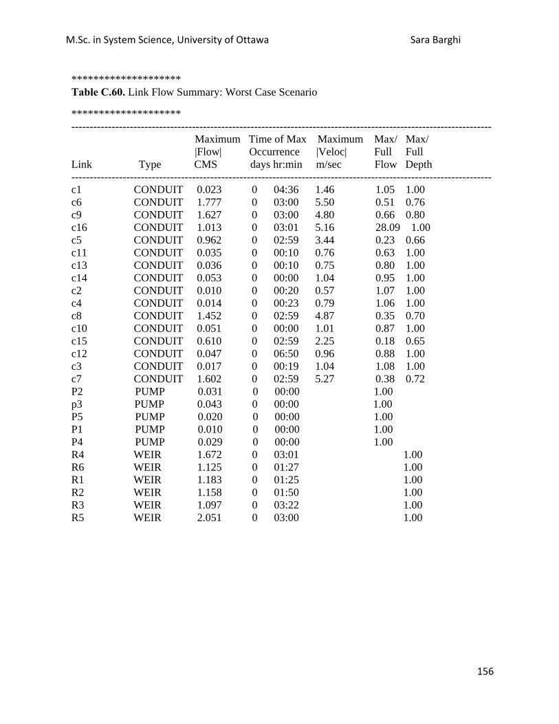
M.Sc. in System Science, University of Ottawa Sara Barghi
156
******************** Table C.60. Link Flow Summary: Worst Case Scenario
******************** ------------------------------------------------------------------------------------------------------------------- Maximum Time of Max Maximum Max/ Max/ |Flow| Occurrence |Veloc| Full Full Link Type CMS days hr:min m/sec Flow Depth ------------------------------------------------------------------------------------------------------------------- c1 CONDUIT 0.023 0 04:36 1.46 1.05 1.00 c6 CONDUIT 1.777 0 03:00 5.50 0.51 0.76 c9 CONDUIT 1.627 0 03:00 4.80 0.66 0.80 c16 CONDUIT 1.013 0 03:01 5.16 28.09 1.00 c5 CONDUIT 0.962 0 02:59 3.44 0.23 0.66 c11 CONDUIT 0.035 0 00:10 0.76 0.63 1.00 c13 CONDUIT 0.036 0 00:10 0.75 0.80 1.00 c14 CONDUIT 0.053 0 00:00 1.04 0.95 1.00 c2 CONDUIT 0.010 0 00:20 0.57 1.07 1.00 c4 CONDUIT 0.014 0 00:23 0.79 1.06 1.00 c8 CONDUIT 1.452 0 02:59 4.87 0.35 0.70 c10 CONDUIT 0.051 0 00:00 1.01 0.87 1.00 c15 CONDUIT 0.610 0 02:59 2.25 0.18 0.65 c12 CONDUIT 0.047 0 06:50 0.96 0.88 1.00 c3 CONDUIT 0.017 0 00:19 1.04 1.08 1.00 c7 CONDUIT 1.602 0 02:59 5.27 0.38 0.72 P2 PUMP 0.031 0 00:00 1.00 p3 PUMP 0.043 0 00:00 1.00 P5 PUMP 0.020 0 00:00 1.00 P1 PUMP 0.010 0 00:00 1.00 P4 PUMP 0.029 0 00:00 1.00 R4 WEIR 1.672 0 03:01 1.00 R6 WEIR 1.125 0 01:27 1.00 R1 WEIR 1.183 0 01:25 1.00 R2 WEIR 1.158 0 01:50 1.00 R3 WEIR 1.097 0 03:22 1.00 R5 WEIR 2.051 0 03:00 1.00

M.Sc. in System Science, University of Ottawa Sara Barghi
157
*************************** Table C.61. Flow Classification Summary: Worst Case Scenario
*************************** ------------------------------------------------------------------------------------------------------------------- Adjusted --- Fraction of Time in Flow Class ---- Avg. Avg. /Actual Up Down Sub Sup Up Down Froude Flow Conduit Length Dry Dry Dry Crit Crit Crit Crit Number Change ------------------------------------------------------------------------------------------------------------------- c1 1.00 0.00 0.00 0.00 0.31 0.69 0.00 0.00 1.30 0.0008 c6 1.00 0.00 0.00 0.00 0.73 0.27 0.00 0.00 0.63 0.0003 c9 1.00 0.00 0.00 0.00 0.75 0.25 0.00 0.00 0.52 0.0004 c16 1.00 0.00 0.00 0.00 1.00 0.00 0.00 0.00 0.52 0.0239 c5 1.00 0.00 0.00 0.00 0.79 0.21 0.00 0.00 0.39 0.0001 c11 1.00 0.00 0.00 0.00 1.00 0.00 0.00 0.00 0.34 0.0005 c13 1.00 0.00 0.00 0.00 1.00 0.00 0.00 0.00 0.31 0.0007 c14 1.00 0.00 0.00 0.00 1.00 0.00 0.00 0.00 0.19 0.0011 c2 1.00 0.00 0.00 0.00 1.00 0.00 0.00 0.00 0.38 0.0007 c4 1.00 0.00 0.00 0.00 1.00 0.00 0.00 0.00 0.19 0.0007 c8 1.00 0.00 0.00 0.00 0.75 0.25 0.00 0.00 0.57 0.0002 c10 1.00 0.00 0.00 0.00 1.00 0.00 0.00 0.00 0.10 0.0011 c15 1.00 0.00 0.00 0.00 0.87 0.13 0.00 0.00 0.25 0.0001 c12 1.00 0.00 0.00 0.00 1.00 0.00 0.00 0.00 0.26 0.0015 c3 1.00 0.00 0.00 0.00 0.34 0.66 0.00 0.00 0.88 0.0007 c7 1.00 0.00 0.00 0.00 0.74 0.26 0.00 0.00 0.62 0.0002 ************************* Table C.62. Conduit Surcharge Summary: Worst Case Scenario
************************* ------------------------------------------------------------------------------------------------------------------- Hours Hours ------------ Hours Full ------------- Above Full Capacity Conduit Both Ends Upstream Dnstream Normal Flow Limited ------------------------------------------------------------------------------------------------------------------- c1 4.11 4.11 4.12 5.26 4.11 c16 3.03 3.03 3.03 23.00 3.03 c11 5.80 5.80 5.81 0.01 0.01 c13 6.15 6.15 6.17 0.01 0.01 c14 1.58 1.58 1.60 0.01 0.01 c2 4.11 4.11 4.12 0.69 0.01 c4 3.38 3.38 3.38 0.45 0.01 c10 3.03 3.03 3.05 0.01 0.01 c12 11.11 11.11 11.13 0.01 0.01 c3 4.38 4.38 4.39 5.56 4.38

M.Sc. in System Science, University of Ottawa Sara Barghi
158
*************** Table C.63. Pumping Summary: Worst Case Scenario
*************** ------------------------------------------------------------------------------------------------------------------- Min Avg Max Total Power % Time Off Percent Number of Flow Flow Flow Volume Usage Pump Curve Pump Utilized Start-Ups CMS CMS CMS 10^6 ltr Kw-hr Low High ------------------------------------------------------------------------------------------------------------------- P2 100.00 1 0.00 0.03 0.03 2.504 9.89 0.0 88.4 P3 100.00 1 0.00 0.04 0.04 3.590 10.77 0.0 94.6 P5 38.82 1 0.00 0.02 0.02 0.643 1.80 0.0 99.9 P1 84.35 2 0.00 0.01 0.01 0.724 2.01 0.0 100.0 P4 100.00 1 0.00 0.03 0.03 2.409 6.31 0.0 100.0 Analysis begun on: Thu May 02 19:41:59 2013 Analysis ended on: Thu May 02 19:41:59 2013 Total elapsed time: < 1 sec
C.4. Precipitation Focus Scenario Simulation Status Report **************** Table C.64. Analysis Options: Precipitation Focus Scenario
**************** Flow Units ............... CMS Process Models: Rainfall/Runoff ........ YES Snowmelt ................. NO Groundwater ............ NO Flow Routing ........... YES Ponding Allowed ..... YES Water Quality .......... YES Infiltration Method ...... ….HORTON Flow Routing Method ...... DYNWAVE Starting Date ............. DEC-14-2010 00:00:00 Ending Date .............. DEC-14-2010 23:00:00 Antecedent Dry Days ...... 5.0 Report Time Step ............ 00:05:00 Wet Time Step ................ 00:05:01 Dry Time Step ............ …00:05:01 Routing Time Step ......... 30.00 sec

M.Sc. in System Science, University of Ottawa Sara Barghi
159
************************** Table C.65. Runoff Quantity Continuity: Precipitation Focus Scenario
************************** Volume Depth hectare-m mm --------- ------- Total Precipitation ...... 17.148 86.000 Evaporation Loss ......... 0.000 0.000 Infiltration Loss ........ 1.436 7.200 Surface Runoff ........... 15.615 78.312 Final Surface Storage .... 0.103 0.517 Continuity Error (%) ..... -0.033 ************************** Table C.66. Runoff Quality Continuity: Precipitation Focus Scenario
************************** TSS Lead kg kg ---------- ---------- Initial Buildup .......... 6111.392 0.000 Surface Buildup .......... 1329.555 1.528 Wet Deposition ........... 0.000 0.000 Sweeping Removal ......... 0.000 0.000 Infiltration Loss ........ 0.000 0.000 BMP Removal .............. 0.000 0.000 Surface Runoff ........... 6111.506 1.528 Remaining Buildup ........ 1329.555 0.000 Continuity Error (%) ..... -0.002 0.000

M.Sc. in System Science, University of Ottawa Sara Barghi
160
************************** Table C.67. Flow Routing Continuity: Precipitation Focus Scenario
************************** Volume Volume hectare-m 10^6 ltr ----------- ----------- Dry Weather Inflow ....... 0.000 0.000 Wet Weather Inflow ....... 15.615 156.148 Groundwater Inflow ....... 0.000 0.000 RDII Inflow .............. 0.000 0.000 External Inflow .......... 0.757 7.574 External Outflow ......... 14.758 147.579 Internal Outflow ......... 0.959 9.588 Storage Losses ........... 0.000 0.000 Initial Stored Volume .... 0.000 0.000 Final Stored Volume ...... 0.616 6.160 Continuity Error (%) ..... 0.241 ****************************** Table C.68. Quality Routing Continuity: Precipitation Focus Scenario
******************************
TSS Lead kg kg ---------- ---------- Dry Weather Inflow ....... 0.000 0.000 Wet Weather Inflow ....... 6109.957 1.527 Groundwater Inflow ....... 0.000 0.000 RDII Inflow .............. 0.000 0.000 External Inflow .......... 0.000 0.000 Internal Flooding ........ 397.202 0.099 External Outflow ......... 4910.381 1.400 Mass Reacted ............. 687.935 0.000 Initial Stored Mass ...... 0.000 0.000 Final Stored Mass ........ 75.605 0.019 Continuity Error (%) ..... 0.636 0.636 *************************** Table C.69. Time-Step Critical Elements: Precipitation Focus Scenario
*************************** Link c7 (20.76%) Link c16 (9.62%)

M.Sc. in System Science, University of Ottawa Sara Barghi
161
******************************** Table C.70. Highest Flow Instability Indexes: Precipitation Focus Scenario
******************************** Link R5 (23) Link R3 (5) Link c12 (2) ************************* Table C.71. Routing Time Step Summary: Precipitation Focus Scenario
************************* Minimum Time Step : 16.34 sec Average Time Step : 27.46 sec Maximum Time Step : 30.00 sec Percent in Steady State : 0.00 Average Iterations per Step: 2.88 *************************** Table C.72. Subcatchment Runoff Summary: Precipitation Focus Scenario
*************************** ------------------------------------------------------------------------------------------------------------------- Total Total Total Total Total Total Peak Runoff Precip Runon Evap Infil Runoff Runoff Runoff Coeff Subcatchment mm mm mm mm mm 10^6 ltr CMS ------------------------------------------------------------------------------------------------------------------- S1 86.00 0.00 0.00 9.12 75.82 19.72 1.34 0.882 S2 86.00 0.00 0.00 9.12 76.58 16.92 1.20 0.891 S13 86.00 0.00 0.00 5.25 80.71 17.97 1.45 0.938 S11 86.00 0.00 0.00 2.73 83.32 3.52 0.31 0.969 S10 86.00 0.00 0.00 2.78 83.26 3.74 0.33 0.968 S9 86.00 0.00 0.00 3.58 82.44 7.39 0.64 0.959 S8 86.00 0.00 0.00 3.70 82.31 8.05 0.69 0.957 S7 86.00 0.00 0.00 4.35 81.64 11.81 1.00 0.949 S6 86.00 0.00 0.00 6.20 79.83 6.82 0.58 0.928 S3 86.00 0.00 0.00 9.12 76.09 18.74 1.29 0.885 S4 86.00 0.00 0.00 9.12 75.34 21.50 1.42 0.876 S5 86.00 0.00 0.00 7.70 78.31 11.07 0.87 0.911 S12 86.00 0.00 0.00 6.96 79.06 8.88 0.73 0.919

M.Sc. in System Science, University of Ottawa Sara Barghi
162
**************************** Table C.73. Subcatchment Washoff Summary: Precipitation Focus Scenario
**************************** ------------------------------------------------ TSS Lead Subcatchment kg kg ------------------------------------------------ S1 193.765 0.048 S2 658.248 0.165 S13 1244.271 0.311 S11 252.094 0.063 S10 267.589 0.067 S9 501.170 0.125 S8 546.426 0.137 S7 323.387 0.081 S6 190.859 0.048 S3 458.710 0.115 S4 531.530 0.133 S5 316.013 0.079 S12 627.445 0.157 ------------------------------------------------ System 6111.506 1.528

M.Sc. in System Science, University of Ottawa Sara Barghi
163
****************** Table C.74. Node Depth Summary: Precipitation Focus Scenario
****************** ------------------------------------------------------------------------------------------------------------------- Average Maximum Maximum Time of Max Depth Depth HGL Occurrence Node Type Meters Meters Meters days hr:min ------------------------------------------------------------------------------------------------------------------- j2 JUNCTION 0.09 0.26 17.94 0 02:59 j4 JUNCTION 0.12 0.32 20.43 0 02:59 j1 JUNCTION 0.13 0.37 22.93 0 02:59 j5 JUNCTION 0.07 0.22 22.17 0 02:59 j16 JUNCTION 0.06 0.20 23.20 0 02:59 j3 JUNCTION 0.10 0.28 16.43 0 02:59 Treatmentplant JUNCTION 1.63 6.70 6.71 0 03:01 j11 JUNCTION 1.13 5.96 7.60 0 02:55 j9 JUNCTION 0.29 1.63 4.02 0 03:23 j7 JUNCTION 0.17 2.88 6.47 0 02:16 j12 JUNCTION 0.90 5.35 7.41 0 03:01 j14 JUNCTION 0.04 0.11 2.54 0 03:13 TreatmentPlantOutfall OUTFALL 0.35 0.50 0.50 0 00:57 Outfall4 OUTFALL 0.85 1.33 1.33 0 18:59 Outfall6 OUTFALL 1.08 1.56 1.33 0 18:59 Outfall1 OUTFALL 0.49 0.97 1.33 0 18:59 Outfall2 OUTFALL 1.40 1.88 1.33 0 18:59 Outfall3 OUTFALL 1.77 2.25 1.33 0 18:59 Outfall5 OUTFALL 1.78 2.26 1.33 0 18:59 j6 STORAGE 1.97 4.84 5.20 0 02:08 j8 STORAGE 2.20 4.69 4.14 0 02:24 j10 STORAGE 2.21 4.04 3.12 0 03:20 j13 STORAGE 2.05 3.40 2.47 0 03:03 j15 STORAGE 1.97 4.50 4.27 0 02:03

M.Sc. in System Science, University of Ottawa Sara Barghi
164
******************* Table C.75. Node Inflow Summary: Precipitation Focus Scenario
******************* ------------------------------------------------------------------------------------------------------------------- Maximum Maximum Lateral Total Lateral Total Time of Max Inflow Inflow Inflow Inflow Occurrence Volume Volume Node Type CMS CMS days hr:min 10^6 ltr 10^6 ltr ------------------------------------------------------------------------------------------------------------------- j2 JUNCTION 1.202 1.224 0 02:59 16.917 17.851 j4 JUNCTION 1.424 1.437 0 02:59 21.501 21.846 j1 JUNCTION 1.341 1.341 0 02:59 19.721 19.722 j5 JUNCTION 0.872 0.872 0 02:59 11.074 11.073 j16 JUNCTION 0.578 0.578 0 02:59 6.818 6.817 j3 JUNCTION 1.293 1.319 0 02:59 18.740 19.768 Treatmentplant JUNCTION 0.965 2.450 0 02:59 11.136 40.868 j11 JUNCTION 0.000 0.043 0 00:59 0.000 3.447 j9 JUNCTION 0.000 0.029 0 00:55 0.000 1.690 j7 JUNCTION 0.000 0.020 0 00:55 0.000 0.694 j12 JUNCTION 0.000 0.057 0 00:50 0.000 2.454 j14 JUNCTION 0.000 0.010 0 00:55 0.000 0.340 TreatmentPlantOutfall OUTFALL 0.000 0.899 0 03:01 0.000 24.217 Outfall4 OUTFALL 0.000 1.461 0 03:01 0.000 19.180 Outfall6 OUTFALL 0.000 1.125 0 02:03 0.000 21.287 Outfall1 OUTFALL 0.000 1.183 0 02:08 0.000 25.078 Outfall2 OUTFALL 0.000 1.158 0 02:24 0.000 22.573 Outfall3 OUTFALL 0.000 0.975 0 03:18 0.000 19.185 Outfall5 OUTFALL 0.000 1.673 0 03:03 0.000 23.633 j6 STORAGE 0.995 2.312 0 02:59 11.815 30.685 j8 STORAGE 0.694 1.928 0 02:59 8.051 26.882 j10 STORAGE 0.000 1.347 0 02:59 0.000 22.859 j13 STORAGE 1.034 1.901 0 02:59 12.404 25.614 j15 STORAGE 1.450 2.027 0 02:59 17.976 25.433

M.Sc. in System Science, University of Ottawa Sara Barghi
165
********************** Table C.76. Node Surcharge Summary: Precipitation Focus Scenario
********************** Surcharging occurs when water rises above the top of the highest conduit. ------------------------------------------------------------------------------------------------------------------ Max. Height Min. Depth Hours Above Crown Below Rim Node Type Surcharged Meters Meters ------------------------------------------------------------------------------------------------------------------ Treatmentplant JUNCTION 3.26 4.111 0.000 j11 JUNCTION 8.81 5.703 0.000 j9 JUNCTION 3.37 1.375 3.738 j7 JUNCTION 2.39 2.630 2.974 j12 JUNCTION 5.38 5.099 0.000 j6 STORAGE 4.79 2.249 0.000 j8 STORAGE 4.48 2.099 0.000 j10 STORAGE 4.00 1.449 0.307 j13 STORAGE 2.31 0.804 1.505 j15 STORAGE 4.14 1.909 0.000 ********************* Table C.77. Node Flooding Summary: Precipitation Focus Scenario
********************* Flooding refers to all water that overflows a node, whether it ponds or not. ------------------------------------------------------------------------------------------------------------------- Total Maximum Maximum Time of Max Flood Ponded Hours Rate Occurrence Volume Depth Node Flooded CMS days hr:min 10^6 ltr Meters ------------------------------------------------------------------------------------------------------------------- Treatmentplant 1.38 0.099 0 02:45 0.312 6.70 j11 0.19 0.003 0 03:02 0.001 5.96 j6 1.88 1.108 0 02:59 4.229 4.84 j8 1.14 0.741 0 02:59 1.946 4.69 j15 1.56 0.892 0 02:59 3.412 4.50

M.Sc. in System Science, University of Ottawa Sara Barghi
166
********************** Table C.78. Storage Volume Summary: Precipitation Focus Scenario
********************** ------------------------------------------------------------------------------------------------------------------- Average Avg E&I Maximum Max Time of Max Maximum Volume Pcnt Pcnt Volume Pcnt Occurrence Outflow Storage Unit 1000 m3 Full Loss 1000 m3 Full days hr:min CMS ------------------------------------------------------------------------------------------------------------------- j6 1.965 41 0 4.840 100 0 02:08 1.203 j8 2.201 47 0 4.690 100 0 02:24 1.187 j10 2.207 51 0 4.040 93 0 03:20 1.018 j13 2.053 42 0 3.395 69 0 03:03 1.699 j15 1.971 44 0 4.500 100 0 02:03 1.135 *********************** Table C.79. Outfall Loading Summary: Precipitation Focus Scenario
*********************** ------------------------------------------------------------------------------------------------------------------- Flow Avg. Max. Total Total Total Freq. Flow Flow Volume TSS Lead Outfall Node Pcnt. CMS CMS 10^6 ltr kg kg ------------------------------------------------------------------------------------------------------------------- TreatmentPlantOutfall 99.90 0.328 0.899 24.217 29.909 0.179 Outfall4 99.97 0.303 1.461 19.180 709.162 0.177 Outfall6 100.00 0.317 1.125 21.287 1189.206 0.297 Outfall1 99.27 0.366 1.183 25.078 407.423 0.102 Outfall2 100.00 0.332 1.158 22.573 1021.144 0.255 Outfall3 100.00 0.274 0.975 19.185 447.253 0.112 Outfall5 100.00 0.368 1.673 23.633 1105.720 0.276 --------------------------------------------------------------------------------------- System 99.88 2.288 8.450 155.153 4909.817 1.399
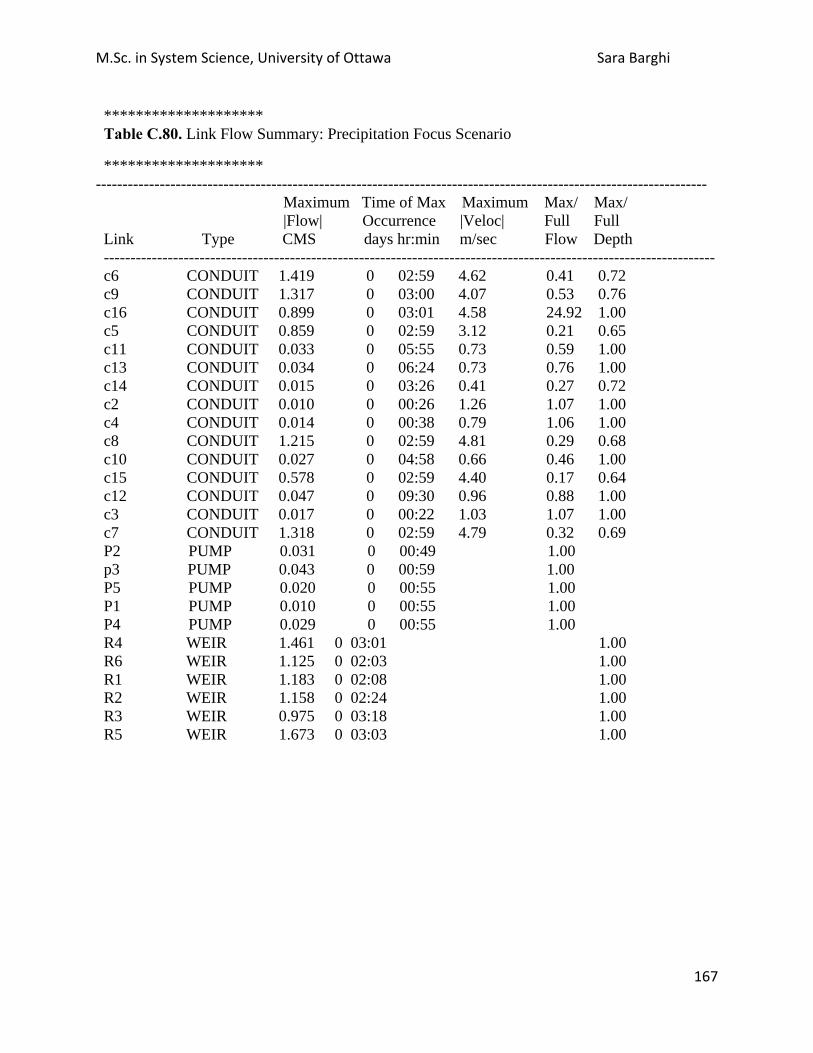
M.Sc. in System Science, University of Ottawa Sara Barghi
167
******************** Table C.80. Link Flow Summary: Precipitation Focus Scenario
******************** ------------------------------------------------------------------------------------------------------------------- Maximum Time of Max Maximum Max/ Max/ |Flow| Occurrence |Veloc| Full Full Link Type CMS days hr:min m/sec Flow Depth ------------------------------------------------------------------------------------------------------------------- c6 CONDUIT 1.419 0 02:59 4.62 0.41 0.72 c9 CONDUIT 1.317 0 03:00 4.07 0.53 0.76 c16 CONDUIT 0.899 0 03:01 4.58 24.92 1.00 c5 CONDUIT 0.859 0 02:59 3.12 0.21 0.65 c11 CONDUIT 0.033 0 05:55 0.73 0.59 1.00 c13 CONDUIT 0.034 0 06:24 0.73 0.76 1.00 c14 CONDUIT 0.015 0 03:26 0.41 0.27 0.72 c2 CONDUIT 0.010 0 00:26 1.26 1.07 1.00 c4 CONDUIT 0.014 0 00:38 0.79 1.06 1.00 c8 CONDUIT 1.215 0 02:59 4.81 0.29 0.68 c10 CONDUIT 0.027 0 04:58 0.66 0.46 1.00 c15 CONDUIT 0.578 0 02:59 4.40 0.17 0.64 c12 CONDUIT 0.047 0 09:30 0.96 0.88 1.00 c3 CONDUIT 0.017 0 00:22 1.03 1.07 1.00 c7 CONDUIT 1.318 0 02:59 4.79 0.32 0.69 P2 PUMP 0.031 0 00:49 1.00 p3 PUMP 0.043 0 00:59 1.00 P5 PUMP 0.020 0 00:55 1.00 P1 PUMP 0.010 0 00:55 1.00 P4 PUMP 0.029 0 00:55 1.00 R4 WEIR 1.461 0 03:01 1.00 R6 WEIR 1.125 0 02:03 1.00 R1 WEIR 1.183 0 02:08 1.00 R2 WEIR 1.158 0 02:24 1.00 R3 WEIR 0.975 0 03:18 1.00 R5 WEIR 1.673 0 03:03 1.00

M.Sc. in System Science, University of Ottawa Sara Barghi
168
*************************** Table C.81. Flow Classification Summary: Precipitation Focus Scenario
*************************** ------------------------------------------------------------------------------------------------------------------- Adjusted --- Fraction of Time in Flow Class ---- Avg. Avg. /Actual Up Down Sub Sup Up Down Froude Flow Conduit Length Dry Dry Dry Crit Crit Crit Crit Number Change ------------------------------------------------------------------------------------------------------------------- c1 1.00 0.00 0.00 0.00 0.33 0.67 0.00 0.00 1.30 0.0008 c6 1.00 0.00 0.00 0.00 0.74 0.26 0.00 0.00 0.61 0.0003 c9 1.00 0.00 0.00 0.00 0.75 0.24 0.00 0.00 0.56 0.0004 c16 1.00 0.00 0.00 0.00 1.00 0.00 0.00 0.00 0.50 0.0171 c5 1.00 0.00 0.00 0.00 0.83 0.17 0.00 0.00 0.36 0.0001 c11 1.00 0.00 0.04 0.00 0.96 0.00 0.00 0.00 0.27 0.0008 c13 1.00 0.00 0.02 0.00 0.98 0.00 0.00 0.00 0.32 0.0008 c14 1.00 0.00 0.04 0.00 0.96 0.00 0.00 0.00 0.11 0.0002 c2 1.00 0.00 0.00 0.00 1.00 0.00 0.00 0.00 0.41 0.0008 c4 1.00 0.00 0.00 0.00 1.00 0.00 0.00 0.00 0.24 0.0008 c8 1.00 0.00 0.00 0.00 0.75 0.25 0.00 0.00 0.60 0.0002 c10 1.00 0.00 0.04 0.00 0.96 0.00 0.00 0.00 0.13 0.0005 c15 1.00 0.00 0.00 0.00 0.92 0.08 0.00 0.00 0.32 0.0001 c12 1.00 0.00 0.02 0.00 0.98 0.00 0.00 0.00 0.33 0.0008 c3 1.00 0.00 0.00 0.00 0.37 0.63 0.00 0.00 0.87 0.0008 c7 1.00 0.00 0.00 0.00 0.72 0.28 0.00 0.00 0.64 0.0002 ************************* Table C.82. Conduit Surcharge Summary: Precipitation Focus Scenario
************************* ------------------------------------------------------------------------------------------------------------------- Hours Hours ------------ Hours Full ------------- Above Full Capacity Conduit Both Ends Upstream Dnstream Normal Flow Limited ------------------------------------------------------------------------------------------------------------------- c1 4.35 4.35 4.36 6.24 4.35 c16 2.61 2.61 2.62 22.86 2.61 c11 3.37 3.37 3.38 0.01 0.01 c13 5.38 5.38 5.38 0.01 0.01 c2 4.35 4.35 4.36 1.15 0.01 c4 3.15 3.15 3.15 0.86 0.01 c10 2.39 2.39 2.40 0.01 0.01 c12 8.81 8.81 8.81 0.01 0.01 c3 4.78 4.78 4.79 6.63 4.78

M.Sc. in System Science, University of Ottawa Sara Barghi
169
*************** Table C.83. Pumping Summary: Precipitation Focus Scenario
*************** ------------------------------------------------------------------------------------------------------------------- Min Avg Max Total Power % Time Off Percent Number of Flow Flow Flow Volume Usage Pump Curve Pump Utilized Start-Ups CMS CMS CMS 10^6 ltr Kw-hr Low High ------------------------------------------------------------------------------------------------------------------- P2 96.45 1 0.00 0.03 0.03 2.440 10.90 0.0 90.9 P3 95.77 1 0.00 0.04 0.04 3.437 11.77 0.0 92.3 P5 41.89 1 0.00 0.02 0.02 0.694 2.10 0.0 100.0 P1 39.58 1 0.00 0.01 0.01 0.340 1.05 0.0 100.0 P4 70.12 2 0.00 0.03 0.03 1.690 4.99 0.0 100.0 Analysis begun on: Fri May 03 14:21:04 2013 Analysis ended on: Fri May 03 14:21:04 2013 Total elapsed time: < 1 sec
C.5. Tide Focus Scenario Simulation Status Report **************** Table C.84. Analysis Options: Tide Focus Scenario
**************** Flow Units ............... CMS Process Models: Rainfall/Runoff ........ YES Snowmelt ................. NO Groundwater ............ NO Flow Routing ........... YES Ponding Allowed ..... YES Water Quality .......... YES Infiltration Method ........... HORTON Flow Routing Method ...... DYNWAVE Starting Date ............. DEC-14-2010 00:00:00 Ending Date .............. DEC-14-2010 23:00:00 Antecedent Dry Days ...... 5.0 Report Time Step ............ 00:05:00 Wet Time Step ................ 00:05:01 Dry Time Step ................ 00:05:01 Routing Time Step ......... 30.00 sec

M.Sc. in System Science, University of Ottawa Sara Barghi
170
************************** Table C.85. Runoff Quantity Continuity: Tide Focus Scenario
************************** Volume Volume hectare-m 10^6 ltr ------------- ------------- Total Precipitation ...... 1.381 6.925 Evaporation Loss ......... 0.000 0.000 Infiltration Loss ........ 0.924 4.636 Surface Runoff ........... 0.413 2.071 Final Surface Storage .... 0.044 0.222 Continuity Error (%) ..... -0.060
************************** Table C.86. Runoff Quality Continuity: Precipitation Focus Scenario
************************** TSS Lead kg kg ---------- ---------- Initial Buildup .......... 6111.392 0.000 Surface Buildup .......... 1.777 0.048 Wet Deposition ........... 0.000 0.000 Sweeping Removal ......... 0.000 0.000 Infiltration Loss ........ 0.000 0.000 BMP Removal .............. 0.000 0.000 Surface Runoff ........... 193.201 0.048 Remaining Buildup ........ 5919.581 0.000 Continuity Error (%) ..... 0.006 0.000

M.Sc. in System Science, University of Ottawa Sara Barghi
171
************************** Table C.87. Flow Routing Continuity: Precipitation Focus Scenario
************************** Volume Volume hectare-m 10^6 ltr ----------- ----------- Dry Weather Inflow ....... 0.000 0.000 Wet Weather Inflow ....... 0.410 4.105 Groundwater Inflow ....... 0.000 0.000 RDII Inflow .............. 0.000 0.000 External Inflow .......... 3.028 30.281 External Outflow ......... 1.994 19.939 Internal Outflow ......... 0.000 0.000 Storage Losses ........... 0.000 0.000 Initial Stored Volume .... 0.000 0.000 Final Stored Volume ...... 1.323 13.233 Continuity Error (%) ..... 3.528 ****************************** Table C.88. Quality Routing Continuity: Precipitation Focus Scenario
******************************
TSS Lead kg kg ---------- ---------- Dry Weather Inflow ....... 0.000 0.000 Wet Weather Inflow ....... 192.455 0.048 Groundwater Inflow ....... 0.000 0.000 RDII Inflow .............. 0.000 0.000 External Inflow .......... 0.000 0.000 Internal Flooding ........ 0.000 0.000 External Outflow ......... 32.331 0.022 Mass Reacted ............. 55.510 0.000 Initial Stored Mass ...... 0.000 0.000 Final Stored Mass ........ 100.753 0.025 Continuity Error (%) ..... 2.006 2.006

M.Sc. in System Science, University of Ottawa Sara Barghi
172
************************* Table C.89. Highest Continuity Errors: Tide Focus Scenario
************************* Node j6 (9.41%) Node j8 (5.61%) Node j15 (5.26%) Node j13 (4.91%) Node j14 (4.13%) *************************** Table C.90. Time-Step Critical Elements: Tide Focus Scenario
*************************** Link c16 (7.58%) ******************************** Table C.91. Highest Flow Instability Indexes: Tide Focus Scenario
******************************** Link R5 (18) Link R3 (6) Link R2 (5)
************************* Table C.92. Routing Time Step Summary: Tide Focus Scenario
************************* Minimum Time Step : 28.10 sec Average Time Step : 29.89 sec Maximum Time Step : 30.00 sec Percent in Steady State : 0.00 Average Iterations per Step: 2.06

M.Sc. in System Science, University of Ottawa Sara Barghi
173
*************************** Table C.93. Subcatchment Runoff Summary: Tide Focus Scenario
*************************** ------------------------------------------------------------------------------------------------------------------- Total Total Total Total Total Total Peak Runoff Precip Runon Evap Infil Runoff Runoff Runoff Coeff Subcatchment mm mm mm mm mm 10^6 ltr CMS ------------------------------------------------------------------------------------------------------------------
S1 6.93 0.00 0.00 5.19 1.56 0.41 0.01 0.225 S2 6.93 0.00 0.00 5.19 1.58 0.35 0.00 0.227 S13 6.93 0.00 0.00 3.46 2.99 0.67 0.01 0.432 S11 6.93 0.00 0.00 3.46 3.28 0.14 0.00 0.474 S10 6.93 0.00 0.00 3.46 3.28 0.15 0.00 0.473 S9 6.93 0.00 0.00 3.46 3.19 0.29 0.00 0.460 S8 6.93 0.00 0.00 3.46 3.17 0.31 0.00 0.458 S7 6.93 0.00 0.00 3.46 3.10 0.45 0.01 0.447 S6 6.93 0.00 0.00 5.19 1.64 0.14 0.00 0.237 S3 6.93 0.00 0.00 5.19 1.57 0.39 0.01 0.226 S4 6.93 0.00 0.00 5.19 1.55 0.44 0.01 0.224 S5 6.93 0.00 0.00 5.19 1.61 0.23 0.00 0.233 S12 6.93 0.00 0.00 5.19 1.63 0.18 0.00 0.235 **************************** Table C.94. Subcatchment Washoff Summary: Tide Focus Scenario
**************************** ------------------------------------------------ TSS Lead Subcatchment kg kg ------------------------------------------------ S1 4.012 0.001 S2 13.769 0.003 S13 49.727 0.012 S11 11.069 0.003 S10 11.728 0.003 S9 21.341 0.005 S8 23.169 0.006 S7 13.386 0.003 S6 4.177 0.001 S3 9.528 0.002 S4 10.932 0.003 S5 6.778 0.002 S12 13.584 0.003 ------------------------------------------------ System 193.201 0.048
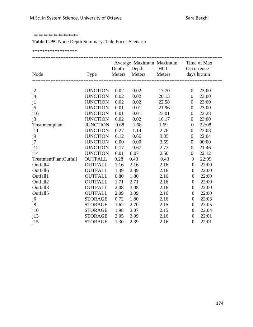
M.Sc. in System Science, University of Ottawa Sara Barghi
174
****************** Table C.95. Node Depth Summary: Tide Focus Scenario
****************** ------------------------------------------------------------------------------------------------------------------- Average Maximum Maximum Time of Max Depth Depth HGL Occurrence Node Type Meters Meters Meters days hr:min -------------------------------------------------------------------------------------------------------------------
j2 JUNCTION 0.02 0.02 17.70 0 23:00 j4 JUNCTION 0.02 0.02 20.13 0 23:00 j1 JUNCTION 0.02 0.02 22.58 0 23:00 j5 JUNCTION 0.01 0.01 21.96 0 23:00 j16 JUNCTION 0.01 0.01 23.01 0 22:28 j3 JUNCTION 0.02 0.02 16.17 0 23:00 Treatmentplant JUNCTION 0.68 1.68 1.69 0 22:08 j11 JUNCTION 0.27 1.14 2.78 0 22:08 j9 JUNCTION 0.12 0.66 3.05 0 22:04 j7 JUNCTION 0.00 0.00 3.59 0 00:00 j12 JUNCTION 0.17 0.67 2.73 0 21:46 j14 JUNCTION 0.01 0.07 2.50 0 22:12 TreatmentPlantOutfall OUTFALL 0.28 0.43 0.43 0 22:09 Outfall4 OUTFALL 1.16 2.16 2.16 0 22:00 Outfall6 OUTFALL 1.39 2.39 2.16 0 22:00 Outfall1 OUTFALL 0.80 1.80 2.16 0 22:00 Outfall2 OUTFALL 1.71 2.71 2.16 0 22:00 Outfall3 OUTFALL 2.08 3.08 2.16 0 22:00 Outfall5 OUTFALL 2.09 3.09 2.16 0 22:00 j6 STORAGE 0.72 1.80 2.16 0 22:03 j8 STORAGE 1.62 2.70 2.15 0 22:05 j10 STORAGE 1.98 3.07 2.15 0 22:04 j13 STORAGE 2.05 3.09 2.16 0 22:01 j15 STORAGE 1.30 2.39 2.16 0 22:01

M.Sc. in System Science, University of Ottawa Sara Barghi
175
******************* Table C.96. Node Inflow Summary: Tide Focus Scenario
******************* ------------------------------------------------------------------------------------------------------------------- Maximum Maximum Lateral Total Lateral Total Time of Max Inflow Inflow Inflow Inflow Occurrence Volume Volume Node Type CMS CMS days hr:min 10^6 ltr 10^6 ltr ------------------------------------------------------------------------------------------------------------------- j2 JUNCTION 0.005 0.006 0 23:00 0.346 0.417 j4 JUNCTION 0.006 0.006 0 23:00 0.440 0.458 j1 JUNCTION 0.005 0.005 0 23:00 0.403 0.403 j5 JUNCTION 0.003 0.003 0 23:00 0.226 0.226 j16 JUNCTION 0.002 0.002 0 22:58 0.139 0.139 j3 JUNCTION 0.005 0.006 0 23:00 0.383 0.455 Treatmentplant JUNCTION 0.006 0.421 0 21:59 0.430 15.554 j11 JUNCTION 0.000 0.043 0 01:35 0.000 3.347 j9 JUNCTION 0.000 0.029 0 09:22 0.000 1.429 j7 JUNCTION 0.000 0.000 0 00:00 0.000 0.000 j12 JUNCTION 0.000 0.031 0 00:46 0.000 2.465 j14 JUNCTION 0.000 0.010 0 19:27 0.000 0.133 TreatmentPlantOutfall OUTFALL 0.000 0.412 0 22:09 0.000 15.250 Outfall4 OUTFALL 0.000 0.335 0 21:59 0.000 8.952 Outfall6 OUTFALL 0.000 0.138 0 00:00 0.000 4.110 Outfall1 OUTFALL 0.000 0.096 0 20:00 0.000 2.743 Outfall2 OUTFALL 0.000 0.236 0 00:00 0.000 5.452 Outfall3 OUTFALL 0.000 0.390 0 00:00 0.000 6.558 Outfall5 OUTFALL 0.000 1.001 0 00:00 0.000 7.154 j6 STORAGE 0.006 0.107 0 20:00 0.446 2.756 j8 STORAGE 0.004 0.236 0 00:00 0.308 5.259 j10 STORAGE 0.000 0.390 0 00:00 0.000 7.535 j13 STORAGE 0.004 1.001 0 00:00 0.320 6.814 j15 STORAGE 0.009 0.138 0 00:00 0.663 3.782

M.Sc. in System Science, University of Ottawa Sara Barghi
176
********************** Table C.97. Node Surcharge Summary: Tide Focus Scenario
********************** Surcharging occurs when water rises above the top of the highest conduit. ------------------------------------------------------------------------------------------------------------------ Max. Height Min. Depth Hours Above Crown Below Rim Node Type Surcharged Meters Meters ------------------------------------------------------------------------------------------------------------------ j11 JUNCTION 3.28 0.883 3.137 j9 JUNCTION 1.97 0.402 4.711 j12 JUNCTION 1.24 0.418 4.676 j8 STORAGE 1.53 0.110 1.989 j10 STORAGE 3.37 0.483 1.273 j13 STORAGE 3.43 0.496 1.813 ********************* Table C.98. Node Flooding Summary: Tide Focus Scenario
********************* No nodes were flooded. ********************** Table C.99. Storage Volume Summary: Tide Focus Scenario
********************** ------------------------------------------------------------------------------------------------------------------- Average Avg E&I Maximum Max Time of Max Maximum Volume Pcnt Pcnt Volume Pcnt Occurrence Outflow Storage Unit 1000 m3 Full Loss 1000 m3 Full days hr:min CMS ------------------------------------------------------------------------------------------------------------------- j6 0.722 15 0 1.795 37 0 22:03 0.048 j8 1.621 35 0 2.701 58 0 22:05 0.087 j10 1.984 46 0 3.074 71 0 22:04 0.116 j13 2.052 42 0 3.087 63 0 22:01 0.128 j15 1.303 29 0 2.387 53 0 22:01 0.071

M.Sc. in System Science, University of Ottawa Sara Barghi
177
*********************** Table C.100. Outfall Loading Summary: Tide Focus Scenario
*********************** ------------------------------------------------------------------------------------------------------------------- Flow Avg. Max. Total Total Total Freq. Flow Flow Volume TSS Lead Outfall Node Pcnt. CMS CMS 10^6 ltr kg kg ------------------------------------------------------------------------------------------------------------------- TreatmentPlantOutfall 99.96 0.185 0.412 15.250 2.534 0.015 Outfall4 100.00 0.109 0.335 8.952 0.140 0.000 Outfall6 100.00 0.050 0.138 4.110 14.663 0.004 Outfall1 100.00 0.033 0.096 2.743 4.980 0.001 Outfall2 99.96 0.066 0.236 5.452 4.916 0.001 Outfall3 100.00 0.079 0.390 6.558 1.982 0.000 Outfall5 100.00 0.086 1.001 7.154 3.122 0.001 ------------------------------------------------------------------------------------------------------------------- System 99.99 0.608 1.883 50.220 32.337 0.022

M.Sc. in System Science, University of Ottawa Sara Barghi
178
******************** Table C.101. Link Flow Summary: Tide Focus Scenario
******************** ------------------------------------------------------------------------------------------------------------------- Maximum Time of Max Maximum Max/ Max/ |Flow| Occurrence |Veloc| Full Full Link Type CMS days hr:min m/sec Flow Depth ------------------------------------------------------------------------------------------------------------------- c1 CONDUIT 0.001 0 23:00 0.65 0.04 0.14 c6 CONDUIT 0.006 0 23:00 0.06 0.00 0.51 c9 CONDUIT 0.004 0 23:00 0.12 0.00 0.52 c16 CONDUIT 0.412 0 22:09 2.16 11.41 0.93 c5 CONDUIT 0.003 0 23:00 0.01 0.00 0.51 c11 CONDUIT 0.030 0 12:36 0.72 0.53 1.00 c13 CONDUIT 0.031 0 23:00 0.70 0.69 1.00 c14 CONDUIT 0.010 0 22:12 0.30 0.19 0.65 c2 CONDUIT 0.000 0 23:00 0.22 0.03 0.13 c4 CONDUIT 0.000 0 23:00 0.21 0.02 0.12 c8 CONDUIT 0.005 0 23:00 0.03 0.00 0.51 c10 CONDUIT 0.000 0 00:00 0.00 0.00 0.50 c15 CONDUIT 0.002 0 20:37 0.01 0.00 0.51 c12 CONDUIT 0.044 0 12:33 0.96 0.83 1.00 c3 CONDUIT 0.001 0 23:00 0.44 0.04 0.14 c7 CONDUIT 0.006 0 23:00 0.03 0.00 0.51 P2 PUMP 0.031 0 00:46 1.00 p3 PUMP 0.043 0 01:35 1.00 P5 PUMP 0.000 0 00:00 0.00 P1 PUMP 0.010 0 19:27 1.00 P4 PUMP 0.029 0 09:22 1.00 R4 WEIR 0.335 0 21:59 0.83 R6 WEIR 0.138 0 00:00 0.92 R1 WEIR 0.096 0 20:00 0.69 R2 WEIR 0.236 0 00:00 1.00 R3 WEIR 0.390 0 00:00 1.00 R5 WEIR 1.001 0 00:00 1.00

M.Sc. in System Science, University of Ottawa Sara Barghi
179
*************************** Table C.102. Flow Classification Summary: Tide Focus Scenario
*************************** ------------------------------------------------------------------------------------------------------------------- Adjusted --- Fraction of Time in Flow Class ---- Avg. Avg. /Actual Up Down Sub Sup Up Down Froude Flow Conduit Length Dry Dry Dry Crit Crit Crit Crit Number Change -------------------------------------------------------------------------------------------------------------------
c1 1.00 0.00 0.00 0.00 0.02 0.98 0.00 0.00 1.67 0.0000 c6 1.00 0.00 0.00 0.00 1.00 0.00 0.00 0.00 0.02 0.0000 c9 1.00 0.00 0.00 0.00 1.00 0.00 0.00 0.00 0.05 0.0000 c16 1.00 0.00 0.00 0.00 1.00 0.00 0.00 0.00 0.57 0.0077 c5 1.00 0.00 0.00 0.00 1.00 0.00 0.00 0.00 0.01 0.0000 c11 1.00 0.00 0.41 0.00 0.59 0.00 0.00 0.00 0.25 0.0002 c13 1.00 0.00 0.03 0.00 0.97 0.00 0.00 0.00 0.43 0.0003 c14 1.00 0.00 0.84 0.00 0.16 0.00 0.00 0.00 0.04 0.0001 c2 1.00 0.00 0.00 0.00 1.00 0.00 0.00 0.00 0.60 0.0000 c4 1.00 0.00 0.00 0.00 1.00 0.00 0.00 0.00 0.59 0.0000 c8 1.00 0.00 0.00 0.00 1.00 0.00 0.00 0.00 0.01 0.0000 c10 1.00 0.00 1.00 0.00 0.00 0.00 0.00 0.00 0.00 0.0000 c15 1.00 0.00 0.00 0.00 1.00 0.00 0.00 0.00 0.01 0.0000 c12 1.00 0.00 0.07 0.00 0.93 0.00 0.00 0.00 0.47 0.0004 c3 1.00 0.00 0.00 0.00 0.04 0.95 0.00 0.00 1.14 0.0000 c7 1.00 0.00 0.00 0.00 1.00 0.00 0.00 0.00 0.02 0.0000 ************************* Table C.103. Conduit Surcharge Summary: Tide Focus Scenario
************************* ------------------------------------------------------------------------------------------------------------------- Hours Hours ------------ Hours Full ------------- Above Full Capacity Conduit Both Ends Upstream Dnstream Normal Flow Limited ------------------------------------------------------------------------------------------------------------------- c16 0.01 0.01 0.01 22.80 0.01 c11 1.96 1.96 1.96 0.01 0.01 c13 1.24 1.24 1.24 0.01 0.01 c12 3.28 3.28 3.28 0.01 0.01

M.Sc. in System Science, University of Ottawa Sara Barghi
180
*************** Table C.104. Pumping Summary: Tide Focus Scenario
*************** ------------------------------------------------------------------------------------------------------------------- Min Avg Max Total Power % Time Off Percent Number of Flow Flow Flow Volume Usage Pump Curve Pump Utilized Start-Ups CMS CMS CMS 10^6 ltr Kw-hr Low High ------------------------------------------------------------------------------------------------------------------- P2 96.67 1 0.00 0.03 0.03 2.465 7.29 0.0 100.0 p3 93.15 1 0.00 0.04 0.04 3.348 7.14 0.0 100.0 P5 0.00 0 0.00 0.00 0.00 0.000 0.00 0.0 0.0 P1 15.48 1 0.00 0.01 0.01 0.133 0.20 0.0 100.0 P4 59.32 1 0.00 0.03 0.03 1.429 4.42 0.0 100.0 Analysis begun on: Sat May 04 13:29:00 2013 Analysis ended on: Sat May 04 13:29:00 2013 Total elapsed time: < 1 sec
C.6. Tide and Initial Depth Focus Scenario Simulation Status Report **************** Table C.105. Analysis Options: Tide and Initial Depth Scenario
**************** Flow Units ............... CMS Process Models: Rainfall/Runoff ........ YES Snowmelt ................. NO Groundwater ............ NO Flow Routing ........... YES Ponding Allowed ..... YES Water Quality .......... YES Infiltration Method ........... HORTON Flow Routing Method ...... DYNWAVE Starting Date ............. DEC-14-2010 00:00:00 Ending Date .............. DEC-14-2010 23:00:00 Antecedent Dry Days ...... 5.0 Report Time Step ............ 00:05:00 Wet Time Step ................ 00:05:01 Dry Time Step ................ 00:05:01 Routing Time Step ......... 30.00 sec

M.Sc. in System Science, University of Ottawa Sara Barghi
181
************************** Table C.106. Runoff Quantity Continuity : Tide and Initial Depth Scenario
************************** Volume Volume hectare-m 10^6 ltr ------------- ------------- Total Precipitation ...... 17.038 85.450 Evaporation Loss ......... 0.000 0.000 Infiltration Loss ........ 1.578 7.915 Surface Runoff ........... 12.984 65.118 Final Surface Storage .... 2.509 12.586 Continuity Error (%) ..... -0.197 ************************** Table C.107. Runoff Quality Continuity: Tide and Initial Depth Scenario ************************** TSS Lead kg kg ---------- ---------- Initial Buildup .......... 6111.392 0.000 Surface Buildup .......... 0.822 1.382 Wet Deposition ........... 0.000 0.000 Sweeping Removal ......... 0.000 0.000 Infiltration Loss ........ 0.000 0.000 BMP Removal .............. 0.000 0.000 Surface Runoff ........... 5515.999 1.379 Remaining Buildup ........ 583.621 0.000 Continuity Error (%) ..... 0.206 0.228

M.Sc. in System Science, University of Ottawa Sara Barghi
182
************************** Table C.108. Flow Routing Continuity: Tide and Initial Depth Scenario ************************** Volume Volume hectare-m 10^6 ltr ----------- ----------- Dry Weather Inflow ....... 0.000 0.000 Wet Weather Inflow ....... 12.883 128.834 Groundwater Inflow ....... 0.000 0.000 RDII Inflow .............. 0.000 0.000 External Inflow .......... 0.173 1.727 External Outflow ......... 12.935 129.354 Internal Outflow ......... 0.000 0.001 Storage Losses ........... 0.000 0.000 Initial Stored Volume .... 1.347 13.472 Final Stored Volume ...... 1.462 14.621 Continuity Error (%) ..... 0.039 ************************** Table C.109. Quality Routing Continuity: Tide and Initial Depth Scenario ************************** TSS Lead kg kg ---------- ---------- Dry Weather Inflow ....... 0.000 0.000 Wet Weather Inflow ....... 5489.545 1.372 Groundwater Inflow ....... 0.000 0.000 RDII Inflow .............. 0.000 0.000 External Inflow .......... 0.000 0.000 Internal Flooding ........ 0.000 0.000 External Outflow ......... 3772.253 1.209 Mass Reacted ............. 1061.953 0.000 Initial Stored Mass ...... 0.000 0.000 Final Stored Mass ........ 614.220 0.154 Continuity Error (%) ..... 0.749 0.749 ************************* Table C.110. Highest Continuity Errors: Tide and Initial Depth Scenario
************************* Node j14 (-2.14%) Node j7 (-1.20%)

M.Sc. in System Science, University of Ottawa Sara Barghi
183
*************************** Table C.111. Time-Step Critical Elements: Tide and Initial DepthScenario
*************************** Link c16 (46.60%) ******************************** Table C.112. Highest Flow Instability Indexes: Tide and Initial DepthScenario
******************************** Link R4 (3) Link R5 (1) Link c16 (1) ************************* Table C.113. Routing Time Step Summary: Tide and Initial DepthScenario
************************* Minimum Time Step : 23.42 sec Average Time Step : 28.84 sec Maximum Time Step : 30.00 sec Percent in Steady State : 0.00 Average Iterations per Step: 2.43 *************************** Table C.114. Subcatchment Runoff Summary: Tide and Initial Depth Scenario *************************** ------------------------------------------------------------------------------------------------------------------- Total Total Total Total Total Total Peak Runoff Precip Runon Evap Infil Runoff Runoff Runoff Coeff Subcatchment mm mm mm mm mm 10^6 ltr CMS ------------------------------------------------------------------------------------------------------------------- S1 85.45 0.00 0.00 8.87 60.37 15.70 0.39 0.707 S2 85.45 0.00 0.00 8.87 61.75 13.64 0.35 0.723 S13 85.45 0.00 0.00 5.91 69.49 15.48 0.45 0.813 S11 85.45 0.00 0.00 5.91 75.47 3.19 0.11 0.883 S10 85.45 0.00 0.00 5.91 75.33 3.38 0.11 0.882 S9 85.45 0.00 0.00 5.91 73.37 6.58 0.21 0.859 S8 85.45 0.00 0.00 5.91 73.07 7.15 0.23 0.855 S7 85.45 0.00 0.00 5.91 71.56 10.36 0.32 0.837 S6 85.45 0.00 0.00 8.87 67.58 5.77 0.17 0.791 S3 85.45 0.00 0.00 8.87 60.85 14.99 0.37 0.712 S4 85.45 0.00 0.00 8.87 59.53 16.99 0.41 0.697 S5 85.45 0.00 0.00 8.87 64.90 9.18 0.25 0.759 S12 85.45 0.00 0.00 8.87 66.22 7.44 0.21 0.775

M.Sc. in System Science, University of Ottawa Sara Barghi
184
**************************** Table C.115. Subcatchment Washoff Summary: Tide and Initial Depth Scenario
****************************
------------------------------------------------ TSS Lead Subcatchment kg kg ------------------------------------------------ S1 156.620 0.039 S2 544.254 0.136 S13 1157.629 0.289 S11 252.086 0.063 S10 267.572 0.067 S9 492.315 0.123 S8 534.616 0.134 S7 309.850 0.077 S6 172.718 0.043 S3 373.710 0.093 S4 423.624 0.106 S5 274.626 0.069 S12 556.379 0.139 ------------------------------------------------ System 5515.999 1.379

M.Sc. in System Science, University of Ottawa Sara Barghi
185
****************** Table C.116. Node Depth Summary: Tide and Initial DepthScenario
****************** ------------------------------------------------------------------------------------------------------------------- Average Maximum Maximum Time of Max Depth Depth HGL Occurrence Node Type Meters Meters Meters days hr:min -------------------------------------------------------------------------------------------------------------------
j2 JUNCTION 0.09 0.14 17.82 0 07:59 j4 JUNCTION 0.11 0.16 20.27 0 08:00 j1 JUNCTION 0.12 0.18 22.74 0 08:00 j5 JUNCTION 0.07 0.12 22.07 0 07:59 j16 JUNCTION 0.07 0.11 23.11 0 07:59 j3 JUNCTION 0.10 0.15 16.30 0 07:59 Treatmentplant JUNCTION 1.35 2.59 2.60 0 00:00 j11 JUNCTION 0.82 5.96 7.60 0 00:00 j9 JUNCTION 0.20 8.14 10.53 0 00:00 j7 JUNCTION 0.09 9.12 12.71 0 00:00 j12 JUNCTION 0.41 8.11 10.17 0 00:00 j14 JUNCTION 0.08 9.89 12.32 0 00:00 TreatmentPlantOutfall OUTFALL 0.39 0.45 0.45 0 22:05 Outfall4 OUTFALL 1.17 2.16 2.16 0 21:59 Outfall6 OUTFALL 1.40 2.39 2.16 0 21:59 Outfall1 OUTFALL 0.81 1.80 2.16 0 21:59 Outfall2 OUTFALL 1.72 2.71 2.16 0 21:59 Outfall3 OUTFALL 2.09 3.08 2.16 0 21:59 Outfall5 OUTFALL 2.10 3.09 2.16 0 21:59 j6 STORAGE 1.83 2.59 2.95 0 00:00 j8 STORAGE 2.06 2.96 2.41 0 23:00 j10 STORAGE 2.21 3.20 2.28 0 23:00 j13 STORAGE 2.14 3.11 2.18 0 22:16 j15 STORAGE 1.92 2.59 2.36 0 00:00

M.Sc. in System Science, University of Ottawa Sara Barghi
186
******************* Table C.117. Node Inflow Summary: Tide and Initial Depth Scenario
******************* ------------------------------------------------------------------------------------------------------------------- Maximum Maximum Lateral Total Lateral Total Time of Max Inflow Inflow Inflow Inflow Occurrence Volume Volume Node Type CMS CMS days hr:min 10^6 ltr 10^6 ltr ------------------------------------------------------------------------------------------------------------------- j2 JUNCTION 0.346 0.368 0 07:59 13.541 15.016 j4 JUNCTION 0.409 0.422 0 07:59 16.862 17.396 j1 JUNCTION 0.385 0.385 0 07:59 15.586 15.582 j5 JUNCTION 0.254 0.254 0 07:59 9.111 9.108 j16 JUNCTION 0.174 0.174 0 07:59 5.730 5.728 j3 JUNCTION 0.372 0.398 0 07:59 14.876 16.484 Treatmentplant JUNCTION 0.321 0.800 0 07:59 9.886 34.058 j11 JUNCTION 0.000 0.043 0 00:00 0.000 3.593 j9 JUNCTION 0.000 0.029 0 00:00 0.000 2.409 j7 JUNCTION 0.000 0.020 0 00:00 0.000 1.345 j12 JUNCTION 0.000 0.031 0 00:00 0.000 2.550 j14 JUNCTION 0.000 0.010 0 00:00 0.000 0.858 TreatmentPlantOutfall OUTFALL 0.000 0.478 0 22:05 0.000 28.183 Outfall4 OUTFALL 0.000 0.698 0 00:00 0.000 7.647 Outfall6 OUTFALL 0.000 0.680 0 00:00 0.000 20.274 Outfall1 OUTFALL 0.000 0.709 0 00:00 0.000 23.406 Outfall2 OUTFALL 0.000 0.609 0 00:00 0.000 20.085 Outfall3 OUTFALL 0.000 0.517 0 00:00 0.000 14.619 Outfall5 OUTFALL 0.000 0.915 0 00:00 0.000 16.867 j6 STORAGE 0.318 0.680 0 07:59 10.275 26.939 j8 STORAGE 0.227 0.605 0 07:59 7.091 25.502 j10 STORAGE 0.000 0.427 0 08:00 0.000 21.467 j13 STORAGE 0.320 0.571 0 07:59 10.551 22.579 j15 STORAGE 0.454 0.627 0 07:59 15.358 23.665

M.Sc. in System Science, University of Ottawa Sara Barghi
187
********************** Table C.118. Node Surcharge Summary: Tide and Initial Depth Scenario
********************** Surcharging occurs when water rises above the top of the highest conduit. ------------------------------------------------------------------------------------------------------------------ Max. Height Min. Depth Hours Above Crown Below Rim Node Type Surcharged Meters Meters ------------------------------------------------------------------------------------------------------------------ j11 JUNCTION 18.60 5.703 0.000 j9 JUNCTION 2.16 7.889 0.000 j7 JUNCTION 0.05 8.871 0.000 j12 JUNCTION 10.21 7.851 0.000 j14 JUNCTION 0.05 9.631 0.000 j8 STORAGE 1.63 0.370 1.729 j10 STORAGE 4.28 0.609 1.147 j13 STORAGE 3.44 0.523 1.786 ********************* Table C.119. Node Flooding Summary: Tide and Initial Depth Scenario ********************* Flooding refers to all water that overflows a node, whether it ponds or not. ------------------------------------------------------------------------------------------------------------------- Total Maximum Maximum Time of Max Flood Ponded Hours Rate Occurrence Volume Depth Node Flooded CMS days hr:min 10^6 ltr Meters ------------------------------------------------------------------------------------------------------------------- j11 0.01 0.019 0 00:00 0.000 5.96 j9 0.01 0.011 0 00:00 0.000 8.14 j7 0.01 0.006 0 00:00 0.000 9.12 j12 0.01 0.005 0 00:00 0.000 8.11 j14 0.01 0.001 0 00:00 0.000 9.89

M.Sc. in System Science, University of Ottawa Sara Barghi
188
********************** Table C.120. Storage Volume Summary: Tide and Initial DepthScenario ********************** ------------------------------------------------------------------------------------------------------------------- Average Avg E&I Maximum Max Time of Max Maximum Volume Pcnt Pcnt Volume Pcnt Occurrence Outflow Storage Unit 1000 m3 Full Loss 1000 m3 Full days hr:min CMS -------------------------------------------------------------------------------------------------------------------
j6 1.829 38 0 2.591 54 0 00:00 0.724 j8 2.063 44 0 2.961 63 0 23:00 0.633 j10 2.212 51 0 3.200 74 0 23:00 0.561 j13 2.139 44 0 3.114 64 0 22:16 0.926 j15 1.916 43 0 2.591 58 0 00:00 0.685 *********************** Table C.121. Outfall Loading Summary: Tide and Initial Depth Scenario
*********************** ------------------------------------------------------------------------------------------------------------------- Flow Avg. Max. Total Total Total Freq. Flow Flow Volume TSS Lead Outfall Node Pcnt. CMS CMS 10^6 ltr kg kg ------------------------------------------------------------------------------------------------------------------- TreatmentPlantOutfall 100.00 0.344 0.478 28.183 27.476 0.272 Outfall4 100.00 0.095 0.698 7.647 257.391 0.064 Outfall6 100.00 0.247 0.680 20.274 1110.925 0.278 Outfall1 100.00 0.285 0.709 23.406 383.864 0.096 Outfall2 100.00 0.245 0.609 20.085 846.998 0.212 Outfall3 100.00 0.178 0.517 14.619 339.895 0.085 Outfall5 100.00 0.206 0.915 16.867 806.692 0.202 ------------------------------------------------------------------------------------------------------------------- System 100.00 1.600 4.299 131.081 3773.241 1.209

M.Sc. in System Science, University of Ottawa Sara Barghi
189
******************** Table C.122. Link Flow Summary: Tide and Initial DepthScenario
******************** ------------------------------------------------------------------------------------------------------------------- Maximum Time of Max Maximum Max/ Max/ |Flow| Occurrence |Veloc| Full Full Link Type CMS days hr:min m/sec Flow Depth ------------------------------------------------------------------------------------------------------------------- c1 CONDUIT 0.023 0 07:59 1.44 1.04 0.96 c6 CONDUIT 0.405 0 08:00 1.58 0.12 0.62 c9 CONDUIT 0.362 0 08:00 1.38 0.15 0.63 c16 CONDUIT 0.478 0 22:05 2.48 13.26 0.95 c5 CONDUIT 0.241 0 08:00 1.01 0.06 0.58 c11 CONDUIT 0.036 0 00:11 0.78 0.63 1.00 c13 CONDUIT 0.040 0 00:12 0.86 0.90 1.00 c14 CONDUIT 0.053 0 00:00 1.04 0.95 1.00 c2 CONDUIT 0.010 0 07:57 0.57 1.07 0.95 c4 CONDUIT 0.012 0 08:00 0.73 0.93 0.88 c8 CONDUIT 0.358 0 08:00 1.44 0.09 0.60 c10 CONDUIT 0.051 0 00:00 1.01 0.87 1.00 c15 CONDUIT 0.174 0 08:00 0.73 0.05 0.58 c12 CONDUIT 0.049 0 00:17 1.02 0.92 1.00 c3 CONDUIT 0.017 0 07:12 1.03 1.07 0.99 c7 CONDUIT 0.398 0 08:00 1.59 0.10 0.60 P2 PUMP 0.031 0 00:00 1.00 p3 PUMP 0.043 0 00:00 1.00 P5 PUMP 0.020 0 00:00 1.00 P1 PUMP 0.010 0 00:00 1.00 P4 PUMP 0.029 0 00:00 1.00 R4 WEIR 0.698 0 00:00 1.00 R6 WEIR 0.680 0 00:00 1.00 R1 WEIR 0.709 0 00:00 1.00 R2 WEIR 0.609 0 00:00 1.00 R3 WEIR 0.517 0 00:00 1.00 R5 WEIR 0.915 0 00:00 1.00
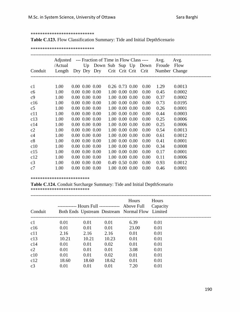
M.Sc. in System Science, University of Ottawa Sara Barghi
190
*************************** Table C.123. Flow Classification Summary: Tide and Initial DepthScenario
*************************** ------------------------------------------------------------------------------------------------------------------- Adjusted --- Fraction of Time in Flow Class ---- Avg. Avg. /Actual Up Down Sub Sup Up Down Froude Flow Conduit Length Dry Dry Dry Crit Crit Crit Crit Number Change -------------------------------------------------------------------------------------------------------------------
c1 1.00 0.00 0.00 0.00 0.26 0.73 0.00 0.00 1.29 0.0013 c6 1.00 0.00 0.00 0.00 1.00 0.00 0.00 0.00 0.45 0.0002 c9 1.00 0.00 0.00 0.00 1.00 0.00 0.00 0.00 0.37 0.0002 c16 1.00 0.00 0.00 0.00 1.00 0.00 0.00 0.00 0.73 0.0195 c5 1.00 0.00 0.00 0.00 1.00 0.00 0.00 0.00 0.26 0.0001 c11 1.00 0.00 0.00 0.00 1.00 0.00 0.00 0.00 0.44 0.0003 c13 1.00 0.00 0.00 0.00 1.00 0.00 0.00 0.00 0.25 0.0006 c14 1.00 0.00 0.00 0.00 1.00 0.00 0.00 0.00 0.25 0.0006 c2 1.00 0.00 0.00 0.00 1.00 0.00 0.00 0.00 0.54 0.0013 c4 1.00 0.00 0.00 0.00 1.00 0.00 0.00 0.00 0.61 0.0012 c8 1.00 0.00 0.00 0.00 1.00 0.00 0.00 0.00 0.41 0.0001 c10 1.00 0.00 0.00 0.00 1.00 0.00 0.00 0.00 0.34 0.0008 c15 1.00 0.00 0.00 0.00 1.00 0.00 0.00 0.00 0.17 0.0001 c12 1.00 0.00 0.00 0.00 1.00 0.00 0.00 0.00 0.11 0.0006 c3 1.00 0.00 0.00 0.00 0.49 0.50 0.00 0.00 0.93 0.0012 c7 1.00 0.00 0.00 0.00 1.00 0.00 0.00 0.00 0.46 0.0001 ************************* Table C.124. Conduit Surcharge Summary: Tide and Initial DepthScenario ************************* ------------------------------------------------------------------------------------------------------------------- Hours Hours ------------ Hours Full ------------- Above Full Capacity Conduit Both Ends Upstream Dnstream Normal Flow Limited ------------------------------------------------------------------------------------------------------------------- c1 0.01 0.01 0.01 6.39 0.01 c16 0.01 0.01 0.01 23.00 0.01 c11 2.16 2.16 2.16 0.01 0.01 c13 10.21 10.21 10.23 0.01 0.01 c14 0.01 0.01 0.02 0.01 0.01 c2 0.01 0.01 0.01 3.08 0.01 c10 0.01 0.01 0.02 0.01 0.01 c12 18.60 18.60 18.62 0.01 0.01 c3 0.01 0.01 0.01 7.20 0.01

M.Sc. in System Science, University of Ottawa Sara Barghi
191
*************** Table C.125. Pumping Summary: Tide and Initial DepthScenario *************** ------------------------------------------------------------------------------------------------------------------- Min Avg Max Total Power % Time Off Percent Number of Flow Flow Flow Volume Usage Pump Curve Pump Utilized Start-Ups CMS CMS CMS 10^6 ltr Kw-hr Low High ------------------------------------------------------------------------------------------------------------------- P2 100.00 1 0.00 0.03 0.03 2.550 8.75 0.0 100.0 P3 100.00 1 0.00 0.04 0.04 3.593 11.41 0.0 100.0 P5 81.21 2 0.00 0.02 0.02 1.345 5.25 0.0 100.0 P1 100.00 1 0.00 0.01 0.01 0.859 1.95 0.0 100.0 P4 100.00 1 0.00 0.03 0.03 2.409 7.10 0.0 100.0 Analysis begun on: Sat May 04 15:28:45 2013 Analysis ended on: Sat May 04 15:28:45 2013 Total elapsed time: < 1 sec
C.7. Regulators and Precipitation Focus Scenario Simulation Status Report **************** Table C.126. Analysis Options: Regulators and Precipitation Focus Scenario
**************** Flow Units ............... CMS Process Models: Rainfall/Runoff ........ YES Snowmelt ................. NO Groundwater ............ NO Flow Routing ........... YES Ponding Allowed ..... YES Water Quality .......... YES Infiltration Method ........... HORTON Flow Routing Method ...... DYNWAVE Starting Date ............. DEC-14-2010 00:00:00 Ending Date .............. DEC-14-2010 23:00:00 Antecedent Dry Days ...... 5.0 Report Time Step ............ 00:05:00 Wet Time Step ................ 00:05:01 Dry Time Step ................ 00:05:01 Routing Time Step ......... 30.00 sec

M.Sc. in System Science, University of Ottawa Sara Barghi
192
************************** Table C.127. Runoff Quantity Continuity: Regulators and Precipitation Focus Scenario ************************** Volume Volume hectare-m 10^6 ltr ------------- ------------- Total Precipitation ...... 17.148 86.000 Evaporation Loss ......... 0.000 0.000 Infiltration Loss ........ 1.436 7.200 Surface Runoff ........... 15.615 78.312 Final Surface Storage .... 0.103 0.517 Continuity Error (%) ..... -0.033 ************************** Table C.128. Runoff Quality Continuity: Regulators and Precipitation Focus Scenario ************************** TSS Lead kg kg ---------- ---------- Initial Buildup .......... 6111.392 0.000 Surface Buildup .......... 1329.555 1.528 Wet Deposition ........... 0.000 0.000 Sweeping Removal ......... 0.000 0.000 Infiltration Loss ........ 0.000 0.000 BMP Removal .............. 0.000 0.000 Surface Runoff ........... 6111.506 1.528 Remaining Buildup ........ 1329.555 0.000 Continuity Error (%) ..... -0.002 0.000 ************************** Table C.129. Flow Routing Continuity: Regulators and Precipitation Focus Scenario ************************** Volume Volume hectare-m 10^6 ltr ----------- ----------- Dry Weather Inflow ....... 0.000 0.000 Wet Weather Inflow ....... 15.615 156.148 Groundwater Inflow ....... 0.000 0.000 RDII Inflow .............. 0.000 0.000 External Inflow .......... 0.000 0.000 External Outflow ......... 3.379 33.794 Internal Outflow ......... 9.791 97.907 Storage Losses ........... 0.000 0.000 Initial Stored Volume .... 0.000 0.000 Final Stored Volume ...... 2.245 22.451 Continuity Error (%) ..... 1.278

M.Sc. in System Science, University of Ottawa Sara Barghi
193
************************** Table C.130. Quality Routing Continuity: Regulators and Precipitation Focus Scenario ************************** TSS Lead kg kg ---------- ---------- Dry Weather Inflow ....... 0.000 0.000 Wet Weather Inflow ....... 6109.955 1.527 Groundwater Inflow ....... 0.000 0.000 RDII Inflow .............. 0.000 0.000 External Inflow .......... 0.000 0.000 Internal Flooding ........ 4050.742 1.013 External Outflow ......... 118.232 0.327 Mass Reacted ............. 1188.055 0.000 Initial Stored Mass ...... 0.000 0.000 Final Stored Mass ........ 646.248 0.162 Continuity Error (%) ..... 1.746 1.746 ************************* Table C.131. Highest Continuity Errors: Regulators and Precipitation Focus Scenario ************************* Node j14 (2.18%) Node j6 (2.05%) Node j13 (2.01%) Node j8 (1.78%) Node j10 (1.71%) *************************** Table C.132. Time-Step Critical Elements: Regulators and Precipitation Focus Scenario *************************** Link c7 (27.87%) Link c16 (6.11%) ******************************** Table C.133. Highest Flow Instability Indexes: Regulators and Precipitation Focus Scenario ******************************** Link c12 (2)

M.Sc. in System Science, University of Ottawa Sara Barghi
194
************************* Table C.134. Routing Time Step Summary: Regulators and Precipitation Focus Scenario ************************* Minimum Time Step : 5.64 sec Average Time Step : 27.22 sec Maximum Time Step : 30.00 sec Percent in Steady State : 0.00 Average Iterations per Step : 2.56 *************************** Table C.135. Subcatchment Runoff Summary: Regulators and Precipitation Focus Scenario *************************** ------------------------------------------------------------------------------------------------------------------- Total Total Total Total Total Total Peak Runoff Precip Runon Evap Infil Runoff Runoff Runoff Coeff Subcatchment mm mm mm mm mm 10^6 ltr CMS ------------------------------------------------------------------------------------------------------------------- S1 86.00 0.00 0.00 9.12 75.82 19.72 1.34 0.882 S2 86.00 0.00 0.00 9.12 76.58 16.92 1.20 0.891 S13 86.00 0.00 0.00 5.25 80.71 17.97 1.45 0.938 S11 86.00 0.00 0.00 2.73 83.32 3.52 0.31 0.969 S10 86.00 0.00 0.00 2.78 83.26 3.74 0.33 0.968 S9 86.00 0.00 0.00 3.58 82.44 7.39 0.64 0.959 S8 86.00 0.00 0.00 3.70 82.31 8.05 0.69 0.957 S7 86.00 0.00 0.00 4.35 81.64 11.81 1.00 0.949 S6 86.00 0.00 0.00 6.20 79.83 6.82 0.58 0.928 S3 86.00 0.00 0.00 9.12 76.09 18.74 1.29 0.885 S4 86.00 0.00 0.00 9.12 75.34 21.50 1.42 0.876 S5 86.00 0.00 0.00 7.70 78.31 11.07 0.87 0.911 S12 86.00 0.00 0.00 6.96 79.06 8.88 0.73 0.919

M.Sc. in System Science, University of Ottawa Sara Barghi
195
**************************** Table C.136. Subcatchment Washoff Summary: Regulators and Precipitation Focus Scenario **************************** ------------------------------------------------ TSS Lead Subcatchment kg kg ------------------------------------------------ S1 193.765 0.048 S2 658.248 0.165 S13 1244.271 0.311 S11 252.094 0.063 S10 267.589 0.067 S9 501.170 0.125 S8 546.426 0.137 S7 323.387 0.081 S6 190.859 0.048 S3 458.710 0.115 S4 531.530 0.133 S5 316.013 0.079 S12 627.445 0.157 ------------------------------------------------ System 6111.506 1.528

M.Sc. in System Science, University of Ottawa Sara Barghi
196
****************** Table C.137. Node Depth Summary: Regulators and Precipitation Focus Scenario ****************** ------------------------------------------------------------------------------------------------------------------- Average Maximum Maximum Time of Max Depth Depth HGL Occurrence Node Type Meters Meters Meters days hr:min ------------------------------------------------------------------------------------------------------------------- j2 JUNCTION 0.09 0.26 17.94 0 02:59 j4 JUNCTION 0.23 2.00 22.11 0 02:31 j1 JUNCTION 0.13 0.37 22.93 0 02:59 j5 JUNCTION 0.07 0.22 22.17 0 02:59 j16 JUNCTION 0.06 0.20 23.20 0 02:59 j3 JUNCTION 0.10 0.28 16.43 0 02:59 Treatmentplant JUNCTION 4.43 20.62 20.63 0 03:01 j11 JUNCTION 1.85 5.96 7.60 0 00:30 j9 JUNCTION 1.74 2.26 4.65 0 01:48 j7 JUNCTION 0.94 3.71 7.30 0 01:36 j12 JUNCTION 2.24 8.11 10.17 0 00:35 j14 JUNCTION 1.42 2.75 5.18 0 01:30 TreatmentPlantOutfall OUTFALL 0.33 0.50 0.50 0 00:29 Outfall4 OUTFALL 0.85 1.33 1.33 0 18:59 Outfall6 OUTFALL 1.08 1.56 1.33 0 18:59 Outfall1 OUTFALL 0.49 0.97 1.33 0 18:59 Outfall2 OUTFALL 1.40 1.88 1.33 0 18:59 Outfall3 OUTFALL 1.77 2.25 1.33 0 18:59 Outfall5 OUTFALL 1.78 2.26 1.33 0 18:59 j6 STORAGE 4.58 4.84 5.20 0 01:31 j8 STORAGE 4.45 4.69 4.14 0 01:36 j10 STORAGE 4.05 4.35 3.43 0 02:04 j13 STORAGE 4.54 4.90 3.97 0 01:39 j15 STORAGE 4.25 4.50 4.27 0 01:28

M.Sc. in System Science, University of Ottawa Sara Barghi
197
******************* Table C.138. Node Inflow Summary: Regulators and Precipitation Focus Scenario ******************* ------------------------------------------------------------------------------------------------------------------- Maximum Maximum Lateral Total Lateral Total Time of Max Inflow Inflow Inflow Inflow Occurrence Volume Volume Node Type CMS CMS days hr:min 10^6 ltr 10^6 ltr ------------------------------------------------------------------------------------------------------------------- j2 JUNCTION 1.202 1.224 0 02:59 16.917 17.851 j4 JUNCTION 1.424 1.426 0 02:59 21.501 21.811 j1 JUNCTION 1.340 1.340 0 02:59 19.721 19.722 j5 JUNCTION 0.872 0.872 0 02:59 11.073 11.073 j16 JUNCTION 0.578 0.578 0 02:59 6.818 6.817 j3 JUNCTION 1.293 1.322 0 02:59 18.740 19.780 Treatmentplant JUNCTION 0.965 2.238 0 02:35 11.135 36.446 j11 JUNCTION 0.000 0.194 0 03:01 0.000 5.021 j9 JUNCTION 0.000 0.029 0 00:54 0.000 2.315 j7 JUNCTION 0.000 0.036 0 01:36 0.000 1.595 j12 JUNCTION 0.000 0.122 0 03:01 0.000 3.212 j14 JUNCTION 0.000 0.034 0 01:29 0.000 0.833 TreatmentPlantOutfall OUTFALL 0.000 1.618 0 03:01 0.000 33.794 Outfall4 OUTFALL 0.000 0.000 0 00:00 0.000 0.000 Outfall6 OUTFALL 0.000 0.000 0 00:00 0.000 0.000 Outfall1 OUTFALL 0.000 0.000 0 00:00 0.000 0.000 Outfall2 OUTFALL 0.000 0.000 0 00:00 0.000 0.000 Outfall3 OUTFALL 0.000 0.000 0 00:00 0.000 0.000 Outfall5 OUTFALL 0.000 0.000 0 00:00 0.000 0.000 j6 STORAGE 0.995 2.312 0 02:59 11.814 30.608 j8 STORAGE 0.694 1.928 0 02:59 8.051 27.138 j10 STORAGE 0.000 1.350 0 02:59 0.000 22.079 j13 STORAGE 1.034 1.914 0 02:59 12.403 23.984 j15 STORAGE 1.449 2.027 0 02:59 17.975 24.796

M.Sc. in System Science, University of Ottawa Sara Barghi
198
********************** Table C.139. Node Surcharge Summary: Regulators and Precipitation Focus Scenario ********************** Surcharging occurs when water rises above the top of the highest conduit. ------------------------------------------------------------------------------------------------------------------ Max. Height Min. Depth Hours Above Crown Below Rim Node Type Surcharged Meters Meters ------------------------------------------------------------------------------------------------------------------ j4 JUNCTION 0.96 1.289 0.000 Treatmentplant JUNCTION 5.13 18.024 0.000 j11 JUNCTION 8.32 5.703 0.000 j9 JUNCTION 21.21 2.004 3.109 j7 JUNCTION 21.40 3.451 2.153 j12 JUNCTION 6.57 7.851 0.000 j14 JUNCTION 21.51 2.493 3.491 j6 STORAGE 21.96 2.249 0.000 j8 STORAGE 21.90 2.099 0.000 j10 STORAGE 21.49 1.756 0.000 j13 STORAGE 21.89 2.309 0.000 j15 STORAGE 21.94 1.909 0.000 ********************* Table C.140. Node Flooding Summary: Regulators and Precipitation Focus Scenario ********************* Flooding refers to all water that overflows a node, whether it ponds or not. ------------------------------------------------------------------------------------------------------------------- Total Maximum Maximum Time of Max Flood Ponded Hours Rate Occurrence Volume Depth Node Flooded CMS days hr:min 10^6 ltr Meters ------------------------------------------------------------------------------------------------------------------- j4 0.67 0.459 0 02:59 0.626 2.00 Treatmentplant 5.07 0.472 0 01:15 3.480 20.62 j11 4.41 0.194 0 03:01 2.228 5.96 j12 3.55 0.122 0 03:01 1.161 8.11 j6 14.34 2.291 0 02:59 23.797 4.84 j8 16.53 1.898 0 02:59 19.729 4.69 j10 15.75 1.306 0 03:00 14.073 4.35 j13 10.38 1.893 0 02:59 16.904 4.90 j15 12.33 2.017 0 02:59 19.374 4.50

M.Sc. in System Science, University of Ottawa Sara Barghi
199
********************** Table C.141. Storage Volume Summary: Regulators and Precipitation Focus Scenario
********************** ------------------------------------------------------------------------------------------------------------------- Average Avg E&I Maximum Max Time of Max Maximum Volume Pcnt Pcnt Volume Pcnt Occurrence Outflow Storage Unit 1000 m3 Full Loss 1000 m3 Full days hr:min CMS ------------------------------------------------------------------------------------------------------------------- j6 4.578 95 0 4.840 100 0 01:31 0.020 j8 4.449 95 0 4.690 100 0 01:36 0.045 j10 4.047 93 0 4.347 100 0 02:04 0.043 j13 4.538 93 0 4.900 100 0 01:39 0.041 j15 4.252 94 0 4.500 100 0 01:28 0.010 *********************** Table C.142. Outfall Loading Summary: Regulators and Precipitation Focus Scenario
*********************** ------------------------------------------------------------------------------------------------------------------- Flow Avg. Max. Total Total Total Freq. Flow Flow Volume TSS Lead Outfall Node Pcnt. CMS CMS 10^6 ltr kg kg ------------------------------------------------------------------------------------------------------------------- TreatmentPlantOutfall 99.93 0.487 1.618 33.794 118.214 0.327 Outfall4 0.00 0.000 0.000 0.000 0.000 0.000 Outfall6 0.00 0.000 0.000 0.000 0.000 0.000 Outfall1 0.00 0.000 0.000 0.000 0.000 0.000 Outfall2 0.00 0.000 0.000 0.000 0.000 0.000 Outfall3 0.00 0.000 0.000 0.000 0.000 0.000 Outfall5 0.00 0.000 0.000 0.000 0.000 0.000 ------------------------------------------------------------------------------------------------------------------- System 14.28 0.487 1.618 33.794 118.214 0.327

M.Sc. in System Science, University of Ottawa Sara Barghi
200
******************** Table C.143. Link Flow Summary: Regulators and Precipitation Focus Scenario ******************** ------------------------------------------------------------------------------------------------------------------- Maximum Time of Max Maximum Max/ Max/ |Flow| Occurrence |Veloc| Full Full Link Type CMS days hr:min m/sec Flow Depth ------------------------------------------------------------------------------------------------------------------- c1 CONDUIT 0.023 0 05:03 2.25 1.05 1.00 c6 CONDUIT 1.284 0 02:35 3.44 0.37 1.00 c9 CONDUIT 1.317 0 03:00 4.07 0.53 0.76 c16 CONDUIT 1.618 0 03:01 8.24 44.86 1.00 c5 CONDUIT 0.870 0 02:59 5.00 0.21 0.66 c11 CONDUIT 0.030 0 01:48 0.71 0.54 1.00 c13 CONDUIT 0.101 0 03:01 1.99 2.26 1.00 c14 CONDUIT 0.024 0 01:29 0.47 0.43 1.00 c2 CONDUIT 0.010 0 00:26 0.57 1.07 1.00 c4 CONDUIT 0.014 0 00:38 0.79 1.06 1.00 c8 CONDUIT 1.214 0 02:59 6.04 0.29 0.68 c10 CONDUIT 0.026 0 01:36 0.53 0.44 1.00 c15 CONDUIT 0.578 0 02:59 4.76 0.17 0.64 c12 CONDUIT 0.150 0 03:01 2.97 2.83 1.00 c3 CONDUIT 0.019 0 03:15 1.06 1.20 1.00 c7 CONDUIT 1.321 0 02:59 7.45 0.3 2 0.69 P2 PUMP 0.031 0 05:16 1.00 p3 PUMP 0.043 0 02:04 1.00 P5 PUMP 0.020 0 00:52 1.00 P1 PUMP 0.010 0 00:53 1.00 P4 PUMP 0.029 0 00:54 1.00 R4 WEIR 0.000 0 00:00 0.00 R6 WEIR 0.000 0 00:00 0.00 R1 WEIR 0.000 0 00:00 0.00 R2 WEIR 0.000 0 00:00 0.00 R3 WEIR 0.000 0 00:00 0.00 R5 WEIR 0.000 0 00:00 0.00

M.Sc. in System Science, University of Ottawa Sara Barghi
201
*************************** Table C.144. Flow Classification Summary: Regulators and Precipitation Focus Scenario
*************************** ------------------------------------------------------------------------------------------------------------------- Adjusted --- Fraction of Time in Flow Class ---- Avg. Avg. /Actual Up Down Sub Sup Up Down Froude Flow Conduit Length Dry Dry Dry Crit Crit Crit Crit Number Change -------------------------------------------------------------------------------------------------------------------
c1 1.00 0.00 0.00 0.00 0.33 0.67 0.00 0.00 1.30 0.0008 c6 1.00 0.00 0.00 0.00 0.81 0.19 0.00 0.00 0.48 0.0003 c9 1.00 0.00 0.00 0.00 0.75 0.25 0.00 0.00 0.57 0.0003 c16 1.00 0.00 0.00 0.00 1.00 0.00 0.00 0.00 0.40 0.0288 c5 1.00 0.00 0.00 0.00 0.81 0.19 0.00 0.00 0.45 0.0001 c11 1.00 0.00 0.04 0.00 0.96 0.00 0.00 0.00 0.02 0.0004 c13 1.00 0.00 0.02 0.00 0.98 0.00 0.00 0.00 0.30 0.0030 c14 1.00 0.00 0.04 0.00 0.96 0.00 0.00 0.00 0.01 0.0005 c2 1.00 0.00 0.00 0.00 1.00 0.00 0.00 0.00 0.42 0.0008 c4 1.00 0.00 0.00 0.00 1.00 0.00 0.00 0.00 0.24 0.0013 c8 1.00 0.00 0.00 0.00 0.74 0.26 0.00 0.00 0.64 0.0002 c10 1.00 0.00 0.04 0.00 0.96 0.00 0.00 0.00 0.01 0.0006 c15 1.00 0.00 0.00 0.00 0.91 0.09 0.00 0.00 0.34 0.0001 c12 1.00 0.00 0.02 0.00 0.98 0.00 0.00 0.00 0.34 0.0031 c3 1.00 0.00 0.00 0.00 0.38 0.62 0.00 0.00 0.89 0.0009 c7 1.00 0.00 0.00 0.00 0.72 0.28 0.00 0.00 0.76 0.0002 ************************* Table C.145. Conduit Surcharge Summary: Regulators and Precipitation Focus Scenario
************************* ------------------------------------------------------------------------------------------------------------------- Hours Hours ------------ Hours Full ------------- Above Full Capacity Conduit Both Ends Upstream Dnstream Normal Flow Limited ------------------------------------------------------------------------------------------------------------------- c1 4.35 4.35 4.36 6.24 4.35 c6 0.96 0.96 0.96 0.01 0.01 c16 5.10 5.10 5.10 22.86 5.10 c11 21.21 21.21 21.21 0.01 0.01 c13 6.57 6.57 6.58 2.95 0.01 c14 21.51 21.51 21.51 0.01 0.01 c2 4.35 4.35 4.36 1.15 0.01 c4 3.15 3.15 3.16 0.85 0.01 c10 21.40 21.40 21.40 0.01 0.01 c12 8.32 8.32 8.33 3.71 0.01 c3 4.78 4.78 4.79 6.63 4.78

M.Sc. in System Science, University of Ottawa Sara Barghi
202
*************** Table C.146. Pumping Summary: Regulators and Precipitation Focus Scenario
*************** ------------------------------------------------------------------------------------------------------------------- Min Avg Max Total Power % Time Off Percent Number of Flow Flow Flow Volume Usage Pump Curve Pump Utilized Start-Ups CMS CMS CMS 10^6 ltr Kw-hr Low High ------------------------------------------------------------------------------------------------------------------- P2 96.07 1 0.00 0.03 0.03 2.290 13.75 0.0 80.2 p3 95.18 1 0.00 0.04 0.04 3.409 19.16 0.0 95.6 P5 96.22 1 0.00 0.02 0.02 1.594 2.45 0.0 100.0 P1 96.16 1 0.00 0.01 0.01 0.826 0.64 0.0 100.0 P4 96.07 1 0.00 0.03 0.03 2.315 1.30 0.0 100.0 Analysis begun on: Sat May 04 16:56:28 2013 Analysis ended on: Sat May 04 16:56:28 2013 Total elapsed time: < 1 sec
C.8. Tide and Impervious Focus Scenario Simulation Status Report **************** Table C.147. Analysis Options: Tide and Impervious Focus Scenario
**************** Flow Units ............... CMS Process Models: Rainfall/Runoff ........ YES Snowmelt ................. NO Groundwater ............ NO Flow Routing ........... YES Ponding Allowed ..... YES Water Quality .......... YES Infiltration Method ........... HORTON Flow Routing Method ...... DYNWAVE Starting Date ............. DEC-14-2010 00:00:00 Ending Date .............. DEC-14-2010 23:00:00 Antecedent Dry Days ...... 5.0 Report Time Step ............ 00:05:00 Wet Time Step ................ 00:05:01 Dry Time Step ................ 00:05:01 Routing Time Step ......... 30.00 sec

M.Sc. in System Science, University of Ottawa Sara Barghi
203
************************** Table C.148. Runoff Quantity Continuity: Tide and Impervious Focus Scenario
************************** Volume Volume hectare-m 10^6 ltr ------------- ------------- Total Precipitation ...... 16.523 82.870 Evaporation Loss ......... 0.000 0.000 Infiltration Loss ........ 0.984 4.933 Surface Runoff ........... 14.035 70.390 Final Surface Storage .... 1.533 7.688 Continuity Error (%) ..... -0.170 ************************** Table C.149. Runoff Quality Continuity: Tide and Impervious Focus Scenario
************************** TSS Lead kg kg ---------- ---------- Initial Buildup .......... 6111.392 0.000 Surface Buildup .......... 0.073 1.470 Wet Deposition ........... 0.000 0.000 Sweeping Removal ......... 0.000 0.000 Infiltration Loss ........ 0.000 0.000 BMP Removal .............. 0.000 0.000 Surface Runoff ........... 5873.368 1.468 Remaining Buildup ........ 231.284 0.000 Continuity Error (%) ..... 0.111 0.116

M.Sc. in System Science, University of Ottawa Sara Barghi
204
************************** Table C.150. Flow Routing Continuity: Tide and Impervious Focus Scenario
************************** Volume Volume hectare-m 10^6 ltr ----------- ----------- Dry Weather Inflow ....... 0.000 0.000 Wet Weather Inflow ....... 13.951 139.514 Groundwater Inflow ....... 0.000 0.000 RDII Inflow .............. 0.000 0.000 External Inflow .......... 0.567 5.674 External Outflow ......... 12.941 129.416 Internal Outflow ......... 0.000 0.000 Storage Losses ........... 0.000 0.000 Initial Stored Volume .... 0.000 0.000 Final Stored Volume ...... 1.437 14.366 Continuity Error (%) ..... 0.968 ************************** Table C.151. Quality Routing Continuity: Tide and Impervious Focus Scenario
************************** TSS Lead kg kg ---------- ---------- Dry Weather Inflow ....... 0.000 0.000 Wet Weather Inflow ....... 5859.851 1.465 Groundwater Inflow ....... 0.000 0.000 RDII Inflow .............. 0.000 0.000 External Inflow .......... 0.000 0.000 Internal Flooding ........ 0.000 0.000 External Outflow ......... 4079.861 1.311 Mass Reacted ............. 1162.651 0.000 Initial Stored Mass ...... 0.000 0.000 Final Stored Mass ........ 579.223 0.145 Continuity Error (%) ..... 0.650 0.650

M.Sc. in System Science, University of Ottawa Sara Barghi
205
************************* Table C.152. Highest Continuity Errors: Tide and Impervious Focus Scenario
************************* Node j13 (1.49%) Node j10 (1.40%) Node j8 (1.25%) Node j6 (1.23%) *************************** Table C.153. Time-Step Critical Elements: Tide and Impervious Focus Scenario
*************************** Link c16 (35.82%) ******************************** Table C.154. Highest Flow Instability Indexes: Tide and Impervious Focus Scenario ******************************** Link R4 (18) Link c16 (7) Link c12 (1) ************************* Table C.155. Routing Time Step Summary: Tide and Impervious Focus Scenario
************************* Minimum Time Step : 18.45 sec Average Time Step : 29.22 sec Maximum Time Step : 30.00 sec Percent in Steady State : 0.00 Average Iterations per Step: 2.11

M.Sc. in System Science, University of Ottawa Sara Barghi
206
*************************** Table C.156. Subcatchment Runoff Summary: Tide and Impervious Focus Scenario
*************************** ------------------------------------------------------------------------------------------------------------------- Total Total Total Total Total Total Peak Runoff Precip Runon Evap Infil Runoff Runoff Runoff Coeff Subcatchment mm mm mm mm mm 10^6 ltr CMS ------------------------------------------------------------------------------------------------------------------- S1 82.87 0.00 0.00 6.08 66.59 17.32 0.24 0.804 S2 82.87 0.00 0.00 6.08 67.55 14.92 0.20 0.815 S13 82.87 0.00 0.00 3.04 73.63 16.40 0.21 0.889 S11 82.87 0.00 0.00 3.04 77.61 3.28 0.04 0.936 S10 82.87 0.00 0.00 3.04 77.52 3.48 0.04 0.935 S9 82.87 0.00 0.00 3.04 76.28 6.84 0.09 0.920 S8 82.87 0.00 0.00 3.04 76.09 7.44 0.09 0.918 S7 82.87 0.00 0.00 3.04 75.07 10.86 0.14 0.906 S6 82.87 0.00 0.00 6.08 71.60 6.11 0.08 0.864 S3 82.87 0.00 0.00 6.08 66.92 16.48 0.23 0.808 S4 82.87 0.00 0.00 6.08 66.00 18.84 0.26 0.796 S5 82.87 0.00 0.00 6.08 69.74 9.86 0.13 0.842 S12 82.87 0.00 0.00 3.04 75.76 8.51 0.11 0.914 **************************** Table C.157. Subcatchment Washoff Summary: Tide and Impervious Focus Scenario **************************** ------------------------------------------------ TSS Lead Subcatchment kg kg ------------------------------------------------ S1 172.835 0.043 S2 595.60 0.149 S13 1227.423 0.307 S11 252.091 0.063 S10 267.586 0.067 S9 501.165 0.125 S8 546.421 0.137 S7 323.359 0.081 S6 183.088 0.046 S3 411.191 0.103 S4 469.944 0.117 S5 295.232 0.074 S12 627.434 0.157 ------------------------------------------------ System 5873.368 1.468

M.Sc. in System Science, University of Ottawa Sara Barghi
207
****************** Table C.158. Node Depth Summary: Tide and Impervious Focus Scenario
****************** ------------------------------------------------------------------------------------------------------------------- Average Maximum Maximum Time of Max Depth Depth HGL Occurrence Node Type Meters Meters Meters days hr:min ------------------------------------------------------------------------------------------------------------------- j2 JUNCTION 0.10 0.11 17.79 0 23:00 j4 JUNCTION 0.12 0.13 20.24 0 23:00 j1 JUNCTION 0.13 0.14 22.70 0 23 :00 j5 JUNCTION 0.08 0.08 22.03 0 23:00 j16 JUNCTION 0.07 0.08 23.08 0 23:00 j3 JUNCTION 0.11 0.12 16.27 0 23:00 Treatmentplant JUNCTION 1.37 2.15 2.16 0 22:01 j11 JUNCTION 0.82 1.60 3.24 0 22:02 j9 JUNCTION 0.17 0.77 3.16 0 22:26 j7 JUNCTION 0.08 0.10 3.69 0 08:13 j12 JUNCTION 0.34 1.07 3.13 0 22:02 j14 JUNCTION 0.05 0.07 2.50 0 09:48 TreatmentPlantOutfall OUTFALL 0.40 0.46 0.46 0 22:01 Outfall4 OUTFALL 1.17 2.16 2.16 0 21:59 Outfall6 OUTFALL 1.40 2.39 2.16 0 21:59 Outfall1 OUTFALL 0.81 1.80 2.16 0 21:59 Outfall2 OUTFALL 1.72 2.71 2.16 0 21:59 Outfall3 OUTFALL 2.09 3.08 2.16 0 21:59 Outfall5 OUTFALL 2.10 3.09 2.16 0 21:59 j6 STORAGE 1.75 2.19 2.55 0 22:43 j8 STORAGE 2.03 2.90 2.35 0 22:38 j10 STORAGE 2.16 3.19 2.27 0 22:27 j13 STORAGE 2.11 3.12 2.19 0 22:07 j15 STORAGE 1.85 2.49 2.26 0 22:21

M.Sc. in System Science, University of Ottawa Sara Barghi
208
******************* Table C.159. Node Inflow Summary: Tide and Impervious Focus Scenario
******************* ------------------------------------------------------------------------------------------------------------------- Maximum Maximum Lateral Total Lateral Total Time of Max Inflow Inflow Inflow Inflow Occurrence Volume Volume Node Type CMS CMS days hr:min 10^6 ltr 10^6 ltr ------------------------------------------------------------------------------------------------------------------- j2 JUNCTION 0.205 0.227 0 23:00 14.833 16.535 j4 JUNCTION 0.264 0.272 0 23:00 18.723 19.312 j1 JUNCTION 0.241 0.241 0 23:00 17.216 17.212 j5 JUNCTION 0.131 0.131 0 23:00 9.804 9.802 j16 JUNCTION 0.079 0.079 0 23:00 6.081 6.079 j3 JUNCTION 0.228 0.253 0 23:00 16.384 18.205 Treatmentplant JUNCTION 0.130 0.501 0 22:02 10.267 34.558 j11 JUNCTION 0.000 0.043 0 01:19 0.000 3.387 j9 JUNCTION 0.000 0.029 0 05:56 0.000 1.788 j7 JUNCTION 0.000 0.020 0 05:53 0.000 1.232 j12 JUNCTION 0.000 0.031 0 00:43 0.000 2.470 j14 JUNCTION 0.000 0.010 0 07:03 0.000 0.596 TreatmentPlantOutfall OUTFALL 0.000 0.479 0 22:01 0.000 28.845 Outfall4 OUTFALL 0.000 0.111 0 16:00 0.000 5.756 Outfall6 OUTFALL 0.000 0.306 0 13:31 0.000 20.256 Outfall1 OUTFALL 0.000 0.342 0 13:54 0.000 22.757 Outfall2 OUTFALL 0.000 0.334 0 13:28 0.000 21.504 Outfall3 OUTFALL 0.000 0.390 0 00:00 0.000 16.333 Outfall5 OUTFALL 0.000 1.001 0 00:00 0.000 19.638 j6 STORAGE 0.139 0.358 0 23:00 10.802 26.392 j8 STORAGE 0.094 0.333 0 23:00 7.401 25.521 j10 STORAGE 0.000 0.390 0 00:00 0.000 21.579 j13 STORAGE 0.149 1.001 0 00:00 11.726 23.522 j15 STORAGE 0.214 0.294 0 23:00 16.306 22.953

M.Sc. in System Science, University of Ottawa Sara Barghi
209
********************** Table C.160. Node Surcharge Summary: Tide and Impervious Focus Scenario
********************** Surcharging occurs when water rises above the top of the highest conduit. ------------------------------------------------------------------------------------------------------------------ Max. Height Min. Depth Hours Above Crown Below Rim Node Type Surcharged Meters Meters ------------------------------------------------------------------------------------------------------------------ j11 JUNCTION 20.62 1.350 2.670 j9 JUNCTION 2.42 0.520 4.593 j12 JUNCTION 9.41 0.815 4.279 j8 STORAGE 1.93 0.309 1.790 j10 STORAGE 3.46 0.601 1.155 j13 STORAGE 3.46 0.529 1.780 ********************* Table C.161. Node Flooding Summary: Tide and Impervious Focus Scenario ********************* No nodes were flooded. ********************** Table C.162. Storage Volume Summary: Tide and Impervious Focus Scenario
********************** ------------------------------------------------------------------------------------------------------------------- Average Avg E&I Maximum Max Time of Max Maximum Volume Pcnt Pcnt Volume Pcnt Occurrence Outflow Storage Unit 1000 m3 Full Loss 1000 m3 Full days hr:min CMS ------------------------------------------------------------------------------------------------------------------- j6 1.750 36 0 2.188 45 0 22:43 0.362 j8 2.029 43 0 2.900 62 0 22:38 0.363 j10 2.159 50 0 3.192 73 0 22:27 0.328 j13 2.110 43 0 3.120 64 0 22:07 0.358 j15 1.847 41 0 2.486 55 0 22:21 0.316

M.Sc. in System Science, University of Ottawa Sara Barghi
210
*********************** Table C.163. Outfall Loading Summary: Tide and Impervious Focus Scenario *********************** ------------------------------------------------------------------------------------------------------------------- Flow Avg. Max. Total Total Total Freq. Flow Flow Volume TSS Lead Outfall Node Pcnt. CMS CMS 10^6 ltr kg kg ------------------------------------------------------------------------------------------------------------------- TreatmentPlantOutfall 99.96 0.351 0.479 28.845 28.983 0.298 Outfall4 100.00 0.068 0.111 5.756 226.279 0.057 Outfall6 100.00 0.245 0.306 20.256 1205.035 0.301 Outfall1 100.00 0.276 0.342 22.757 412.139 0.103 Outfall2 100.00 0.260 0.334 21.504 936.839 0.234 Outfall3 100.00 0.197 0.390 16.333 371.068 0.093 Outfall5 100.00 0.237 1.001 19.638 900.380 0.225 ------------------------------------------------------------------------------------------------------------------- System 99.99 1.634 2.042 135.089 4080.723 1.311

M.Sc. in System Science, University of Ottawa Sara Barghi
211
******************** Table C.164. Link Flow Summary: Tide and Impervious Focus Scenario
******************** ------------------------------------------------------------------------------------------------------------------- Maximum Time of Max Maximum Max/ Max/ |Flow| Occurrence |Veloc| Full Full Link Type CMS days hr:min m/sec Flow Depth ------------------------------------------------------------------------------------------------------------------- c1 CONDUIT 0.022 0 23:00 1.43 1.03 0.83 c6 CONDUIT 0.256 0 23:00 1.05 0.07 0.59 c9 CONDUIT 0.219 0 23:00 1.20 0.09 0.60 c16 CONDUIT 0.479 0 22:01 2.48 13.30 0.96 c5 CONDUIT 0.123 0 23:00 0.54 0.03 0.56 c11 CONDUIT 0.030 0 12:53 0.72 0.53 1.00 c13 CONDUIT 0.033 0 16:02 0.70 0.74 1.00 c14 CONDUIT 0.010 0 09:49 0.30 0.19 0.65 c2 CONDUIT 0.008 0 23:00 0.55 0.87 0.75 c4 CONDUIT 0.008 0 23:00 0.58 0.59 0.70 c8 CONDUIT 0.219 0 23:00 0.92 0.05 0.58 c10 CONDUIT 0.020 0 08:13 0.53 0.34 0.70 c15 CONDUIT 0.079 0 23:00 0.35 0.02 0.55 c12 CONDUIT 0.043 0 22:07 0.91 0.82 1.00 c3 CONDUIT 0.016 0 23:00 1.02 1.01 0.82 c7 CONDUIT 0.253 0 23:00 1.05 0.06 0.58 P2 PUMP 0.031 0 00:43 1.00 p3 PUMP 0.043 0 01:19 1.00 P5 PUMP 0.020 0 05:53 1.00 P1 PUMP 0.010 0 07:03 1.00 P4 PUMP 0.029 0 05:56 1.00 R4 WEIR 0.111 0 16:00 0.83 R6 WEIR 0.306 0 13:31 0.96 R1 WEIR 0.342 0 13:54 0.84 R2 WEIR 0.334 0 13:28 1.00 R3 WEIR 0.390 0 00:00 1.00 R5 WEIR 1.001 0 00:00 1.00

M.Sc. in System Science, University of Ottawa Sara Barghi
212
*************************** Table C.165. Flow Classification Summary: Tide and Impervious Focus Scenario
*************************** ------------------------------------------------------------------------------------------------------------------- Adjusted --- Fraction of Time in Flow Class ---- Avg. Avg. /Actual Up Down Sub Sup Up Down Froude Flow Conduit Length Dry Dry Dry Crit Crit Crit Crit Number Change ------------------------------------------------------------------------------------------------------------------- c1 1.00 0.00 0.00 0.00 0.00 1.00 0.00 0.00 1.28 0.0004 c6 1.00 0.00 0.00 0.00 1.00 0.00 0.00 0.00 0.49 0.0000 c9 1.00 0.00 0.00 0.00 0.96 0.04 0.00 0.00 0.48 0.0000 c16 1.00 0.00 0.00 0.00 1.00 0.00 0.00 0.00 0.74 0.0059 c5 1.00 0.00 0.00 0.00 1.00 0.00 0.00 0.00 0.28 0.0000 c11 1.00 0.00 0.25 0.00 0.75 0.00 0.00 0.00 0.31 0.0002 c13 1.00 0.00 0.03 0.00 0.97 0.00 0.00 0.00 0.24 0.0004 c14 1.00 0.00 0.30 0.00 0.70 0.00 0.00 0.00 0.18 0.0001 c2 1.00 0.00 0.00 0.00 1.00 0.00 0.00 0.00 0.55 0.0003 c4 1.00 0.00 0.00 0.00 1.00 0.00 0.00 0.00 0.61 0.0002 c8 1.00 0.00 0.00 0.00 1.00 0.00 0.00 0.00 0.45 0.0000 c10 1.00 0.00 0.25 0.00 0.75 0.00 0.00 0.00 0.31 0.0001 c15 1.00 0.00 0.00 0.00 1.00 0.00 0.00 0.00 0.20 0.0000 c12 1.00 0.00 0.06 0.00 0.94 0.00 0.00 0.00 0.02 0.0003 c3 1.00 0.00 0.00 0.00 0.79 0.21 0.00 0.00 0.94 0.0004 c7 1.00 0.00 0.00 0.00 1.00 0.00 0.00 0.00 0.51 0.0000 ************************* Table C.166. Conduit Surcharge Summary: Tide and Impervious Focus Scenario
************************* ------------------------------------------------------------------------------------------------------------------- Hours Hours ------------ Hours Full ------------- Above Full Capacity Conduit Both Ends Upstream Dnstream Normal Flow Limited ------------------------------------------------------------------------------------------------------------------- c1 0.01 0.01 0.01 16.07 0.01 c16 0.01 0.01 0.01 22.81 0.01 c11 2.42 2.42 2.42 0.01 0.01 c13 9.41 9.41 9.42 0.01 0.01 c12 20.62 20.62 20.62 0.01 0.01 c3 0.01 0.01 0.01 11.43 0.01

M.Sc. in System Science, University of Ottawa Sara Barghi
213
*************** Table C.167. Pumping Summary: Tide and Impervious Focus Scenario
*************** ------------------------------------------------------------------------------------------------------------------- Min Avg Max Total Power % Time Off Percent Number of Flow Flow Flow Volume Usage Pump Curve Pump Utilized Start-Ups CMS CMS CMS 10^6 ltr Kw-hr Low High ------------------------------------------------------------------------------------------------------------------- P2 96.88 1 0.00 0.03 0.03 2.471 8.11 0.0 100.0 p3 94.28 1 0.00 0.04 0.04 3.388 11.02 0.0 100.0 P5 74.42 1 0.00 0.02 0.02 1.232 4.57 0.0 100.0 P1 69.38 1 0.00 0.01 0.01 0.596 1.10 0.0 100.0 P4 74.24 1 0.00 0.03 0.03 1.789 4.52 0.0 100.0 Analysis begun on: Sat May 04 19:44:54 2013 Analysis ended on: Sat May 04 19:44:54 2013 Total elapsed time: < 1 sec
C.9. Depth and Precipitation Focus Scenario Simulation Status Report **************** Table C.168. Analysis Options: Depth and Precipitation Focus Scenario
**************** Flow Units ............... CMS Process Models: Rainfall/Runoff ........ YES Snowmelt ................. NO Groundwater ............ NO Flow Routing ........... YES Ponding Allowed ..... YES Water Quality .......... YES Infiltration Method ........... HORTON Flow Routing Method ...... DYNWAVE Starting Date ............. DEC-14-2010 00:00:00 Ending Date .............. DEC-14-2010 23:00:00 Antecedent Dry Days ...... 5.0 Report Time Step ............ 00:05:00 Wet Time Step ................ 00:05:01 Dry Time Step ................ 00:05:01 Routing Time Step ......... 30.00 sec

M.Sc. in System Science, University of Ottawa Sara Barghi
214
************************** Table C.169. Runoff Quantity Continuity: Depth and Precipitation Focus Scenario
************************** Volume Volume hectare-m 10^6 ltr ------------- ------------- Total Precipitation ...... 17.148 86.000 Evaporation Loss ......... 0.000 0.000 Infiltration Loss ........ 1.436 7.200 Surface Runoff ........... 15.615 78.312 Final Surface Storage .... 0.103 0.517 Continuity Error (%) ..... -0.033 ************************** Table C.170. Runoff Quality Continuity: Depth and Precipitation Focus Scenario
************************** TSS Lead kg kg ---------- ---------- Initial Buildup .......... 6111.392 0.000 Surface Buildup .......... 1329.555 1.528 Wet Deposition ........... 0.000 0.000 Sweeping Removal ......... 0.000 0.000 Infiltration Loss ........ 0.000 0.000 BMP Removal .............. 0.000 0.000 Surface Runoff ........... 6111.506 1.528 Remaining Buildup ........ 1329.555 0.000 Continuity Error (%) ..... -0.002 0.000

M.Sc. in System Science, University of Ottawa Sara Barghi
215
************************** Table C.171. Flow Routing Continuity: Depth and Precipitation Focus Scenario
************************** Volume Volume hectare-m 10^6 ltr ----------- ----------- Dry Weather Inflow ....... 0.000 0.000 Wet Weather Inflow ....... 15.615 156.147 Groundwater Inflow ....... 0.000 0.000 RDII Inflow .............. 0.000 0.000 External Inflow .......... 0.630 6.304 External Outflow ......... 16.008 160.087 Internal Outflow ......... 1.073 10.726 Storage Losses ........... 0.000 0.000 Initial Stored Volume .... 1.347 13.472 Final Stored Volume ...... 0.616 6.163 Continuity Error (%) ..... -0.598 ************************** Table C.172. Quality Routing Continuity: Depth and Precipitation Focus Scenario ************************** TSS Lead kg kg ---------- ---------- Dry Weather Inflow ....... 0.000 0.000 Wet Weather Inflow ....... 6109.954 1.527 Groundwater Inflow ....... 0.000 0.000 RDII Inflow .............. 0.000 0.000 External Inflow .......... 0.000 0.000 Internal Flooding ........ 430.286 0.108 External Outflow ......... 4927.432 1.405 Mass Reacted ............. 691.675 0.000 Initial Stored Mass ...... 0.000 0.000 Final Stored Mass ........ 75.596 0.019 Continuity Error (%) ..... -0.246 -0.246 ************************* Table C.173. Highest Continuity Errors: Depth and Precipitation Focus Scenario
************************* Node j14 (-6.39%) Node j7 (-3.33%)

M.Sc. in System Science, University of Ottawa Sara Barghi
216
*************************** Table C.174. Time-Step Critical Elements: Depth and Precipitation Focus Scenario *************************** Link c7 (20.29%) Link c16 (10.18%) ******************************** Table C.175. Highest Flow Instability Indexes: Depth and Precipitation Focus Scenario ******************************** Link R5 (23) Link R3 (6) ************************* Table C.176. Routing Time Step Summary: Depth and Precipitation Focus Scenario ************************* Minimum Time Step : 16.34 sec Average Time Step : 27.45 sec Maximum Time Step : 30.00 sec Percent in Steady State : 0.00 Average Iterations per Step: 3.01 *************************** Table C.177. Subcatchment Runoff Summary: Depth and Precipitation Focus Scenario *************************** ------------------------------------------------------------------------------------------------------------------- Total Total Total Total Total Total Peak Runoff Precip Runon Evap Infil Runoff Runoff Runoff Coeff Subcatchment mm mm mm mm mm 10^6 ltr CMS ------------------------------------------------------------------------------------------------------------------- S1 86.00 0.00 0.00 9.12 75.82 19.72 1.34 0.882 S2 86.00 0.00 0.00 9.12 76.58 16.92 1.20 0.891 S13 86.00 0.00 0.00 5.25 80.71 17.97 1.45 0.938 S11 86.00 0.00 0.00 2.73 83.32 3.52 0.31 0.969 S10 86.00 0.00 0.00 2.78 83.26 3.74 0.33 0.968 S9 86.00 0.00 0.00 3.58 82.44 7.39 0.64 0.959 S8 86.00 0.00 0.00 3.70 82.31 8.05 0.69 0.957 S7 86.00 0.00 0.00 4.35 81.64 11.81 1.00 0.949 S6 86.00 0.00 0.00 6.20 79.83 6.82 0.58 0.928 S3 86.00 0.00 0.00 9.12 76.09 18.74 1.29 0.885 S4 86.00 0.00 0.00 9.12 75.34 21.50 1.42 0.876 S5 86.00 0.00 0.00 7.70 78.31 11.07 0.87 0.911 S12 86.00 0.00 0.00 6.96 79.06 8.88 0.73 0.919

M.Sc. in System Science, University of Ottawa Sara Barghi
217
**************************** Table C.178. Subcatchment Washoff Summary: Depth and Precipitation Focus Scenario **************************** ------------------------------------------------ TSS Lead Subcatchment kg kg ------------------------------------------------ S1 193.765 0.048 S2 658.248 0.165 S13 1244.271 0.311 S11 252.094 0.063 S10 267.589 0.067 S9 501.170 0.125 S8 546.426 0.137 S7 323.387 0.081 S6 190.859 0.048 S3 458.710 0.115 S4 531.530 0.133 S5 316.013 0.079 S12 627.445 0.157 ------------------------------------------------ System 6111.506 1.528

M.Sc. in System Science, University of Ottawa Sara Barghi
218
****************** Table C.179. Node Depth Summary: Depth and Precipitation Focus Scenario ****************** ------------------------------------------------------------------------------------------------------------------- Average Maximum Maximum Time of Max Depth Depth HGL Occurrence Node Type Meters Meters Meters days hr:min ------------------------------------------------------------------------------------------------------------------- j2 JUNCTION 0.09 0.26 17.94 0 02:59 j4 JUNCTION 0.12 0.32 20.43 0 02:59 j1 JUNCTION 0.13 0.37 22.93 0 02:59 j5 JUNCTION 0.07 0.22 22.17 0 02:59 j16 JUNCTION 0.06 0.20 23.20 0 02:59 j3 JUNCTION 0.10 0.28 16.43 0 02:59 Treatmentplant JUNCTION 1.65 6.70 6.71 0 03:01 j11 JUNCTION 1.19 5.96 7.60 0 00:00 j9 JUNCTION 0.31 8.14 10.53 0 00:00 j7 JUNCTION 0.19 9.12 12.71 0 00:00 j12 JUNCTION 0.94 8.11 10.17 0 00:00 j14 JUNCTION 0.04 9.89 12.32 0 00:00 TreatmentPlantOutfall OUTFALL 0.35 0.50 0.50 0 00:53 Outfall4 OUTFALL 0.85 1.33 1.33 0 19:00 Outfall6 OUTFALL 1.08 1.56 1.33 0 19:00 Outfall1 OUTFALL 0.49 0.97 1.33 0 19:00 Outfall2 OUTFALL 1.40 1.88 1.33 0 19:00 Outfall3 OUTFALL 1.77 2.25 1.33 0 19:00 Outfall5 OUTFALL 1.78 2.26 1.33 0 19:00 j6 STORAGE 2.08 4.84 5.20 0 01:57 j8 STORAGE 2.31 4.69 4.14 0 02:15 j10 STORAGE 2.31 4.09 3.17 0 03:19 j13 STORAGE 2.10 3.40 2.47 0 03:03 j15 STORAGE 2.08 4.50 4.27 0 01:52

M.Sc. in System Science, University of Ottawa Sara Barghi
219
******************* Table C.180. Node Inflow Summary: Depth and Precipitation Focus Scenario ******************* ------------------------------------------------------------------------------------------------------------------- Maximum Maximum Lateral Total Lateral Total Time of Max Inflow Inflow Inflow Inflow Occurrence Volume Volume Node Type CMS CMS days hr:min 10^6 ltr 10^6 ltr ------------------------------------------------------------------------------------------------------------------- j2 JUNCTION 1.202 1.224 0 02:59 16.917 17.849 j4 JUNCTION 1.424 1.437 0 02:59 21.501 21.846 j1 JUNCTION 1.341 1.341 0 02:59 19.721 19.722 j5 JUNCTION 0.872 0.872 0 02:59 11.074 11.073 j16 JUNCTION 0.578 0.578 0 02:59 6.818 6.817 j3 JUNCTION 1.293 1.319 0 02:59 18.740 19.768 Treatmentplant JUNCTION 0.965 2.450 0 02:59 11.136 41.107 j11 JUNCTION 0.000 0.043 0 00:00 0.000 3.590 j9 JUNCTION 0.000 0.029 0 00:00 0.000 1.786 j7 JUNCTION 0.000 0.020 0 00:00 0.000 0.760 j12 JUNCTION 0.000 0.031 0 00:00 0.000 2.530 j14 JUNCTION 0.000 0.010 0 00:00 0.000 0.374 TreatmentPlantOutfall OUTFALL 0.000 0.899 0 03:01 0.000 24.569 Outfall4 OUTFALL 0.000 1.461 0 03:01 0.000 19.560 Outfall6 OUTFALL 0.000 1.125 0 01:53 0.000 23.601 Outfall1 OUTFALL 0.000 1.183 0 01:58 0.000 27.517 Outfall2 OUTFALL 0.000 1.158 0 02:15 0.000 24.927 Outfall3 OUTFALL 0.000 0.985 0 03:17 0.000 21.243 Outfall5 OUTFALL 0.000 1.673 0 03:03 0.000 24.972 j6 STORAGE 0.995 2.312 0 02:59 11.815 33.268 j8 STORAGE 0.694 1.928 0 02:59 8.051 29.449 j10 STORAGE 0.000 1.347 0 02:59 0.000 25.188 j13 STORAGE 1.034 1.901 0 02:59 12.404 27.507 j15 STORAGE 1.450 2.027 0 02:59 17.976 27.986

M.Sc. in System Science, University of Ottawa Sara Barghi
220
********************** Table C.181. Node Surcharge Summary: Depth and Precipitation Focus Scenario ********************** Surcharging occurs when water rises above the top of the highest conduit. ------------------------------------------------------------------------------------------------------------------ Max. Height Min. Depth Hours Above Crown Below Rim Node Type Surcharged Meters Meters ------------------------------------------------------------------------------------------------------------------ Treatmentplant JUNCTION 3.36 4.111 0.000 j11 JUNCTION 9.40 5.703 0.000 j9 JUNCTION 3.59 7.889 0.000 j7 JUNCTION 2.62 8.871 0.000 j12 JUNCTION 5.88 7.851 0.000 j14 JUNCTION 0.05 9.631 0.000 j6 STORAGE 5.24 2.249 0.000 j8 STORAGE 4.96 2.099 0.000 j10 STORAGE 4.33 1.501 0.255 j13 STORAGE 2.36 0.805 1.504 j15 STORAGE 4.55 1.909 0.000 ********************* Table C.182. Node Flooding Summary: Depth and Precipitation Focus Scenario ********************* Flooding refers to all water that overflows a node, whether it ponds or not. ------------------------------------------------------------------------------------------------------------------- Total Maximum Maximum Time of Max Flood Ponded Hours Rate Occurrence Volume Depth Node Flooded CMS days hr:min 10^6 ltr Meters ------------------------------------------------------------------------------------------------------------------- Treatmentplant 1.38 0.099 0 02:45 0.313 6.70 j11 0.19 0.019 0 00:00 0.001 5.96 j9 0.01 0.011 0 00:00 0.000 8.14 j7 0.01 0.006 0 00:00 0.000 9.12 j12 0.01 0.005 0 00:00 0.000 8.11 j14 0.01 0.001 0 00:00 0.000 9.89 j6 2.05 1.108 0 02:59 4.681 4.84 j8 1.29 0.741 0 02:59 2.239 4.69 j15 1.73 0.892 0 02:59 3.804 4.50

M.Sc. in System Science, University of Ottawa Sara Barghi
221
********************** Table C.183. Storage Volume Summary: Depth and Precipitation Focus Scenario ********************** ------------------------------------------------------------------------------------------------------------------- Average Avg E&I Maximum Max Time of Max Maximum Volume Pcnt Pcnt Volume Pcnt Occurrence Outflow Storage Unit 1000 m3 Full Loss 1000 m3 Full days hr:min CMS ------------------------------------------------------------------------------------------------------------------- j6 2.077 43 0 4.840 100 0 01:57 1.203 j8 2.309 49 0 4.690 100 0 02:15 1.187 j10 2.311 53 0 4.092 94 0 03:19 1.029 j13 2.096 43 0 3.396 69 0 03:03 1.699 j15 2.075 46 0 4.500 100 0 01:52 1.135 *********************** Table C.184. Outfall Loading Summary: Depth and Precipitation Focus Scenario *********************** ------------------------------------------------------------------------------------------------------------------- Flow Avg. Max. Total Total Total Freq. Flow Flow Volume TSS Lead Outfall Node Pcnt. CMS CMS 10^6 ltr kg kg ------------------------------------------------------------------------------------------------------------------- TreatmentPlantOutfall 100.00 0.332 0.899 24.569 30.286 0.181 Outfall4 100.00 0.308 1.461 19.560 718.760 0.180 Outfall6 100.00 0.349 1.125 23.601 1185.633 0.296 Outfall1 100.00 0.397 1.183 27.517 408.570 0.102 Outfall2 100.00 0.364 1.158 24.927 1023.624 0.256 Outfall3 100.00 0.303 0.985 21.243 450.868 0.113 Outfall5 99.97 0.386 1.673 24.972 1109.183 0.277 --------------------------------------------------------------------------------------- System 100.00 2.439 8.463 166.389 4926.923 1.405

M.Sc. in System Science, University of Ottawa Sara Barghi
222
******************** Table C.185. Link Flow Summary: Depth and Precipitation Focus Scenario ******************** ------------------------------------------------------------------------------------------------------------------- Maximum Time of Max Maximum Max/ Max/ |Flow| Occurrence |Veloc| Full Full Link Type CMS days hr:min m/sec Flow Depth ------------------------------------------------------------------------------------------------------------------- c1 CONDUIT 0.023 0 05:03 1.45 1.05 1.00 c6 CONDUIT 1.419 0 02:59 4.62 0.41 0.72 c9 CONDUIT 1.317 0 03:00 4.07 0.53 0.76 c16 CONDUIT 0.899 0 03:01 4.58 24.92 1.00 c5 CONDUIT 0.859 0 02:59 3.12 0.21 0.65 c11 CONDUIT 0.036 0 00:10 0.78 0.64 1.00 c13 CONDUIT 0.037 0 00:10 0.76 0.83 1.00 c14 CONDUIT 0.053 0 00:00 1.04 0.95 1.00 c2 CONDUIT 0.010 0 00:26 0.56 1.07 1.00 c4 CONDUIT 0.014 0 00:38 0.79 1.06 1.00 c8 CONDUIT 1.215 0 02:59 4.19 0.29 0.68 c10 CONDUIT 0.051 0 00:00 1.01 0.87 1.00 c15 CONDUIT 0.578 0 02:59 2.15 0.17 0.64 c12 CONDUIT 0.047 0 09:31 0.96 0.88 1.00 c3 CONDUIT 0.017 0 00:22 1.03 1.07 1.00 c7 CONDUIT 1.318 0 02:59 4.48 0.32 0.69 P2 PUMP 0.031 0 00:00 1.00 p3 PUMP 0.043 0 00:00 1.00 P5 PUMP 0.020 0 00:00 1.00 P1 PUMP 0.010 0 00:00 1.00 P4 PUMP 0.029 0 00:00 1.00 R4 WEIR 1.461 0 03:01 1.00 R6 WEIR 1.125 0 01:53 1.00 R1 WEIR 1.183 0 01:58 1.00 R2 WEIR 1.158 0 02:15 1.00 R3 WEIR 0.985 0 03:17 1.00 R5 WEIR 1.673 0 03:03 1.00

M.Sc. in System Science, University of Ottawa Sara Barghi
223
*************************** Table C.186. Flow Classification Summary: Depth and Precipitation Focus Scenario *************************** ------------------------------------------------------------------------------------------------------------------- Adjusted --- Fraction of Time in Flow Class ---- Avg. Avg. /Actual Up Down Sub Sup Up Down Froude Flow Conduit Length Dry Dry Dry Crit Crit Crit Crit Number Change ------------------------------------------------------------------------------------------------------------------- c1 1.00 0.00 0.00 0.00 0.33 0.67 0.00 0.00 1.29 0.0008 c6 1.00 0.00 0.00 0.00 0.74 0.25 0.00 0.00 0.60 0.0003 c9 1.00 0.00 0.00 0.00 0.78 0.22 0.00 0.00 0.48 0.0004 c16 1.00 0.00 0.00 0.00 1.00 0.00 0.00 0.00 0.50 0.0203 c5 1.00 0.00 0.00 0.00 0.83 0.16 0.00 0.00 0.35 0.0001 c11 1.00 0.00 0.00 0.00 1.00 0.00 0.00 0.00 0.29 0.0009 c13 1.00 0.00 0.00 0.00 1.00 0.00 0.00 0.00 0.32 0.0006 c14 1.00 0.00 0.00 0.00 1.00 0.00 0.00 0.00 0.12 0.0008 c2 1.00 0.00 0.00 0.00 1.00 0.00 0.00 0.00 0.40 0.0008 c4 1.00 0.00 0.00 0.00 1.00 0.00 0.00 0.00 0.23 0.0008 c8 1.00 0.00 0.00 0.00 0.77 0.23 0.00 0.00 0.52 0.0002 c10 1.00 0.00 0.00 0.00 1.00 0.00 0.00 0.00 0.14 0.0009 c15 1.00 0.00 0.00 0.00 0.93 0.06 0.00 0.00 0.23 0.0001 c12 1.00 0.00 0.00 0.00 1.00 0.00 0.00 0.00 0.33 0.0004 c3 1.00 0.00 0.00 0.00 0.38 0.62 0.00 0.00 0.87 0.0008 c7 1.00 0.00 0.00 0.00 0.75 0.25 0.00 0.00 0.57 0.0002 ************************* Table C.187. Conduit Surcharge Summary: Depth and Precipitation Focus Scenario ************************* ------------------------------------------------------------------------------------------------------------------- Hours Hours ------------ Hours Full ------------- Above Full Capacity Conduit Both Ends Upstream Dnstream Normal Flow Limited ------------------------------------------------------------------------------------------------------------------- c1 4.35 4.35 4.36 6.23 4.35 c16 2.67 2.67 2.67 23.00 2.67 c11 3.59 3.59 3.60 0.01 0.01 c13 5.88 5.88 5.90 0.01 0.01 c14 0.01 0.01 0.02 0.01 0.01 c2 4.35 4.35 4.36 1.15 0.01 c4 3.15 3.15 3.15 0.86 0.01 c10 2.58 2.58 2.59 0.01 0.01 c12 9.40 9.40 9.41 0.01 0.01 c3 4.77 4.77 4.78 6.63 4.77

M.Sc. in System Science, University of Ottawa Sara Barghi
224
*************** Table C.188. Pumping Summary: Depth and Precipitation Focus Scenario *************** ------------------------------------------------------------------------------------------------------------------- Min Avg Max Total Power % Time Off Percent Number of Flow Flow Flow Volume Usage Pump Curve Pump Utilized Start-Ups CMS CMS CMS 10^6 ltr Kw-hr Low High ------------------------------------------------------------------------------------------------------------------- P2 100.00 1 0.00 0.03 0.03 2.530 11.34 0.0 91.5 p3 100.00 1 0.00 0.04 0.04 3.590 12.36 0.0 93.6 P5 45.87 1 0.00 0.02 0.02 0.760 2.25 0.0 99.9 P1 43.59 1 0.00 0.01 0.01 0.374 1.12 0.0 99.9 P4 74.10 2 0.00 0.03 0.03 1.785 5.13 0.0 100.0 Analysis begun on: Sun May 05 12:35:51 2013 Analysis ended on: Sun May 05 12:35:51 2013 Total elapsed time: < 1 sec
C.10. Initial Depth and Impervious Focus Scenario Simulation Status Report **************** Table C.189. Analysis Options: Initial Depth and Impervious Focus Scenario **************** Flow Units ............... CMS Process Models: Rainfall/Runoff ........ YES Snowmelt ................. NO Groundwater ............ NO Flow Routing ........... YES Ponding Allowed ..... YES Water Quality .......... YES Infiltration Method ........... HORTON Flow Routing Method ...... DYNWAVE Starting Date ............. DEC-14-2010 00:00:00 Ending Date .............. DEC-14-2010 23:00:00 Antecedent Dry Days ...... 5.0 Report Time Step ............ 00:05:00 Wet Time Step ................ 00:05:01 Dry Time Step ................ 00:05:01 Routing Time Step ......... 30.00 sec

M.Sc. in System Science, University of Ottawa Sara Barghi
225
************************** Table C.190. Runoff Quantity Continuity: Initial Depth and Impervious Focus Scenario ************************** Volume Volume hectare-m 10^6 ltr ------------- ------------- Total Precipitation ...... 17.148 86.000 Evaporation Loss ......... 0.000 0.000 Infiltration Loss ........ 0.776 3.891 Surface Runoff ........... 16.362 82.061 Final Surface Storage .... 0.016 0.082 Continuity Error (%) ..... -0.039 ************************** Table C.191. Runoff Quality Continuity: Initial Depth and Impervious Focus Scenario ************************** TSS Lead kg kg ---------- ---------- Initial Buildup .......... 6111.392 0.000 Surface Buildup .......... 1768.215 1.528 Wet Deposition ........... 0.000 0.000 Sweeping Removal ......... 0.000 0.000 Infiltration Loss ........ 0.000 0.000 BMP Removal .............. 0.000 0.000 Surface Runoff ........... 6111.496 1.528 Remaining Buildup ........ 1768.215 0.000 Continuity Error (%) ..... -0.001 0.000 ************************** Table C.192. Flow Routing Continuity: Initial Depth and Impervious Focus Scenario ************************** Volume Volume hectare-m 10^6 ltr ----------- ----------- Dry Weather Inflow ....... 0.000 0.000 Wet Weather Inflow ....... 16.362 163.625 Groundwater Inflow ....... 0.000 0.000 RDII Inflow .............. 0.000 0.000 External Inflow .......... 0.645 6.449 External Outflow ......... 15.617 156.173 Internal Outflow ......... 2.236 22.362 Storage Losses ........... 0.000 0.000 Initial Stored Volume .... 1.347 13.472 Final Stored Volume ...... 0.608 6.080 Continuity Error (%) ..... -0.582

M.Sc. in System Science, University of Ottawa Sara Barghi
226
************************** Table C.193. Quality Routing Continuity: Initial Depth and Impervious Focus Scenario ************************** TSS Lead kg kg ---------- ---------- Dry Weather Inflow ....... 0.000 0.000 Wet Weather Inflow ....... 6109.401 1.527 Groundwater Inflow ....... 0.000 0.000 RDII Inflow .............. 0.000 0.000 External Inflow .......... 0.000 0.000 Internal Flooding ........ 850.378 0.213 External Outflow ......... 4668.206 1.310 Mass Reacted ............. 571.599 0.000 Initial Stored Mass ...... 0.000 0.000 Final Stored Mass ........ 36.950 0.009 Continuity Error (%) ..... -0.290 -0.290 ************************* Table C.194. Highest Continuity Errors: Initial Depth and Impervious Focus Scenario ************************* Node j14 (-8.33%) Node j7 (-4.02%) Node j9 (-1.01%) *************************** Table C.195. Time-Step Critical Elements: Initial Depth and Impervious Focus Scenario *************************** Link c7 (23.64%) Link c16 (6.13%) ******************************** Table C.196. Highest Flow Instability Indexes: Initial Depth and Impervious Focus Scenario ******************************** Link R5 (23) Link R3 (2) ************************* Table C.197. Routing Time Step Summary: Initial Depth and Impervious Focus Scenario ************************* Minimum Time Step : 14.57 sec Average Time Step : 26.74 sec Maximum Time Step : 30.00 sec Percent in Steady State : 0.00 Average Iterations per Step: 2.93

M.Sc. in System Science, University of Ottawa Sara Barghi
227
*************************** Table C.198. Subcatchment Runoff Summary: Initial Depth and Impervious Focus Scenario *************************** ------------------------------------------------------------------------------------------------------------------- Total Total Total Total Total Total Peak Runoff Precip Runon Evap Infil Runoff Runoff Runoff Coeff Subcatchment mm mm mm mm mm 10^6 ltr CMS ------------------------------------------------------------------------------------------------------------------- S1 86.00 0.00 0.00 5.63 80.32 20.89 1.65 0.934 S2 86.00 0.00 0.00 5.23 80.73 17.83 1.44 0.939 S13 86.00 0.00 0.00 1.95 83.92 18.69 1.60 0.976 S11 86.00 0.00 0.00 1.12 84.92 3.59 0.31 0.987 S10 86.00 0.00 0.00 1.13 84.90 3.81 0.33 0.987 S9 86.00 0.00 0.00 1.39 84.60 7.59 0.65 0.984 S8 86.00 0.00 0.00 1.43 84.55 8.27 0.71 0.983 S7 86.00 0.00 0.00 1.65 84.29 12.20 1.05 0.980 S6 86.00 0.00 0.00 3.51 82.51 7.05 0.61 0.959 S3 86.00 0.00 0.00 5.49 80.46 19.82 1.58 0.936 S4 86.00 0.00 0.00 5.87 80.07 22.85 1.78 0.931 S5 86.00 0.00 0.00 4.31 81.68 11.55 0.97 0.950 S12 86.00 0.00 0.00 1.50 84.47 9.49 0.82 0.982 **************************** Table C.199. Subcatchment Washoff Summary: Initial Depth and Impervious Focus Scenario **************************** ------------------------------------------------ TSS Lead Subcatchment kg kg ------------------------------------------------ S1 193.765 0.048 S2 658.247 0.165 S13 1244.27 0.311 S11 252.091 0.063 S10 267.586 0.067 S9 501.170 0.125 S8 546.426 0.137 S7 323.388 0.081 S6 190.858 0.048 S3 458.710 0.115 S4 531.530 0.133 S5 316.011 0.079 S12 627.442 0.157 ------------------------------------------------ System 6111.496 1.528

M.Sc. in System Science, University of Ottawa Sara Barghi
228
****************** Table C.200. Node Depth Summary: Initial Depth and Impervious Focus Scenario
****************** ------------------------------------------------------------------------------------------------------------------- Average Maximum Maximum Time of Max Depth Depth HGL Occurrence Node Type Meters Meters Meters days hr:min ------------------------------------------------------------------------------------------------------------------- j2 JUNCTION 0.09 0.29 17.97 0 03:00 j4 JUNCTION 0.12 0.37 20.48 0 03:00 j1 JUNCTION 0.13 0.42 22.98 0 03:00 j5 JUNCTION 0.07 0.23 22.18 0 03:00 j16 JUNCTION 0.06 0.21 23.21 0 03:00 j3 JUNCTION 0.10 0.31 16.46 0 03:00 Treatmentplant JUNCTION 1.98 8.39 8.40 0 03:00 j11 JUNCTION 1.45 5.96 7.60 0 00:00 j9 JUNCTION 0.44 8.14 10.53 0 00:00 j7 JUNCTION 0.23 9.12 12.71 0 00:00 j12 JUNCTION 1.36 8.11 10.17 0 00:00 j14 JUNCTION 0.19 9.89 12.32 0 00:00 TreatmentPlantOutfall OUTFALL 0.33 0.50 0.50 0 00:33 Outfall4 OUTFALL 0.87 1.28 1.28 0 01:59 Outfall6 OUTFALL 1.10 1.51 1.28 0 01:59 Outfall1 OUTFALL 0.51 0.92 1.28 0 01:59 Outfall2 OUTFALL 1.39 1.88 1.33 0 18:59 Outfall3 OUTFALL 1.76 2.25 1.33 0 18:59 Outfall5 OUTFALL 1.80 2.21 1.28 0 01:59 j6 STORAGE 2.01 4.84 5.20 0 01:25 j8 STORAGE 2.36 4.69 4.14 0 01:35 j10 STORAGE 2.43 4.35 3.43 0 02:20 j13 STORAGE 2.24 4.66 3.73 0 03:01 j15 STORAGE 2.02 4.50 4.27 0 01:24

M.Sc. in System Science, University of Ottawa Sara Barghi
229
******************* Table C.201. Node Inflow Summary: Initial Depth and Impervious Focus Scenario
******************* ------------------------------------------------------------------------------------------------------------------- Maximum Maximum Lateral Total Lateral Total Time of Max Inflow Inflow Inflow Inflow Occurrence Volume Volume Node Type CMS CMS days hr:min 10^6 ltr 10^6 ltr ------------------------------------------------------------------------------------------------------------------- j2 JUNCTION 1.440 1.462 0 03:00 17.834 18.57 j4 JUNCTION 1.782 1.795 0 03:00 22.851 23.136 j1 JUNCTION 1.651 1.651 0 03:00 20.891 20.891 j5 JUNCTION 0.975 0.975 0 03:00 11.551 11.550 j16 JUNCTION 0.610 0.610 0 03:00 7.047 7.046 j3 JUNCTION 1.577 1.603 0 03:00 19.817 20.636 Treatmentplant JUNCTION 0.982 2.783 0 03:00 11.404 41.712 j11 JUNCTION 0.000 0.081 0 03:01 0.000 3.674 j9 JUNCTION 0.000 0.029 0 00:00 0.000 1.674 j7 JUNCTION 0.000 0.024 0 01:30 0.000 0.629 j12 JUNCTION 0.000 0.031 0 00:00 0.000 2.518 j14 JUNCTION 0.000 0.020 0 01:25 0.000 0.294 TreatmentPlantOutfall OUTFALL 0.000 1.013 0 03:00 0.000 22.699 Outfall4 OUTFALL 0.000 1.673 0 03:00 0.000 21.059 Outfall6 OUTFALL 0.000 1.116 0 03:37 0.000 21.637 Outfall1 OUTFALL 0.000 1.183 0 01:25 0.000 25.307 Outfall2 OUTFALL 0.000 1.158 0 01:35 0.000 23.569 Outfall3 OUTFALL 0.000 1.066 0 02:20 0.000 21.385 Outfall5 OUTFALL 0.000 1.984 0 03:02 0.000 26.964 j6 STORAGE 1.050 2.678 0 03:00 12.199 34.937 j8 STORAGE 0.713 2.185 0 03:00 8.271 30.595 j10 STORAGE 0.000 1.632 0 03:00 0.000 26.378 j13 STORAGE 1.126 2.099 0 03:00 13.081 29.161 j15 STORAGE 1.598 2.208 0 03:00 18.690 28.828

M.Sc. in System Science, University of Ottawa Sara Barghi
230
********************** Table C.202. Node Surcharge Summary: Initial Depth and Impervious Focus Scenario
********************** Surcharging occurs when water rises above the top of the highest conduit. ------------------------------------------------------------------------------------------------------------------ Max. Height Min. Depth Hours Above Crown Below Rim Node Type Surcharged Meters Meters ------------------------------------------------------------------------------------------------------------------ Treatmentplant JUNCTION 3.52 5.798 0.000 j11 JUNCTION 6.72 5.703 0.000 j9 JUNCTION 4.04 7.889 0.000 j7 JUNCTION 3.05 8.871 0.000 j12 JUNCTION 5.11 7.851 0.000 j14 JUNCTION 2.29 9.631 0.000 j6 STORAGE 5.01 2.249 0.000 j8 STORAGE 4.77 2.099 0.000 j10 STORAGE 4.53 1.756 0.000 j13 STORAGE 3.61 2.064 0.245 j15 STORAGE 4.48 1.909 0.000 ********************* Table C.203. Node Flooding Summary: Initial Depth and Impervious Focus Scenario ********************* Flooding refers to all water that overflows a node, whether it ponds or not. ------------------------------------------------------------------------------------------------------------------- Total Maximum Maximum Time of Max Flood Ponded Hours Rate Occurrence Volume Depth Node Flooded CMS days hr:min 10^6 ltr Meters ------------------------------------------------------------------------------------------------------------------- Treatmentplant 2.49 0.140 0 01:29 0.699 8.39 j11 1.65 0.081 0 03:01 0.273 5.96 j9 0.01 0.011 0 00:00 0.000 8.14 j7 0.01 0.006 0 00:00 0.000 9.12 j12 0.01 0.005 0 00:00 0.000 8.11 j14 0.01 0.001 0 00:00 0.000 9.89 j6 2.48 1.474 0 03:00 8.866 4.84 j8 1.93 0.998 0 03:00 5.118 4.69 j10 1.07 0.548 0 03:00 1.477 4.35 j15 2.14 1.104 0 03:00 6.626 4.50

M.Sc. in System Science, University of Ottawa Sara Barghi
231
********************** Table C.204. Storage Volume Summary: Initial Depth and Impervious Focus Scenario ********************** ------------------------------------------------------------------------------------------------------------------- Average Avg E&I Maximum Max Time of Max Maximum Volume Pcnt Pcnt Volume Pcnt Occurrence Outflow Storage Unit 1000 m3 Full Loss 1000 m3 Full days hr:min CMS ------------------------------------------------------------------------------------------------------------------- j6 2.010 42 0 4.840 100 0 01:25 1.203 j8 2.357 50 0 4.690 100 0 01:35 1.187 j10 2.434 56 0 4.347 100 0 02:20 1.110 j13 2.238 46 0 4.655 95 0 03:01 2.008 j15 2.022 45 0 4.500 100 0 01:24 1.126 *********************** Table C.205. Outfall Loading Summary: Initial Depth and Impervious Focus Scenario *********************** ------------------------------------------------------------------------------------------------------------------- Flow Avg. Max. Total Total Total Freq. Flow Flow Volume TSS Lead Outfall Node Pcnt. CMS CMS 10^6 ltr kg kg ------------------------------------------------------------------------------------------------------------------- TreatmentPlantOutfall 100.00 0.336 1.013 22.699 34.931 0.152 Outfall4 100.00 0.373 1.673 21.059 774.330 0.194 Outfall6 100.00 0.346 1.116 21.637 1025.849 0.256 Outfall1 100.00 0.395 1.183 25.307 346.655 0.087 Outfall2 100.00 0.372 1.158 23.569 908.229 0.227 Outfall3 100.00 0.331 1.066 21.385 425.167 0.106 Outfall5 100.00 0.465 1.984 26.964 1152.315 0.288 --------------------------------------------------------------------------------------- System 100.00 2.618 9.144 162.621 4667.476 1.310

M.Sc. in System Science, University of Ottawa Sara Barghi
232
******************** Table C.206. Link Flow Summary: Initial Depth and Impervious Focus Scenario ******************** ------------------------------------------------------------------------------------------------------------------- Maximum Time of Max Maximum Max/ Max/ |Flow| Occurrence |Veloc| Full Full Link Type CMS days hr:min m/sec Flow Depth ------------------------------------------------------------------------------------------------------------------- c1 CONDUIT 0.023 0 04:36 1.46 1.05 1.00 c6 CONDUIT 1.777 0 03:00 5.49 0.51 0.76 c9 CONDUIT 1.627 0 03:00 4.80 0.66 0.80 c16 CONDUIT 1.013 0 03:00 5.16 28.10 1.00 c5 CONDUIT 0.962 0 03:00 3.44 0.23 0.66 c11 CONDUIT 0.036 0 00:10 0.78 0.64 1.00 c13 CONDUIT 0.035 0 00:10 0.75 0.78 1.00 c14 CONDUIT 0.053 0 00:00 1.04 0.95 1.00 c2 CONDUIT 0.010 0 00:21 0.57 1.07 1.00 c4 CONDUIT 0.014 0 00:24 0.79 1.06 1.00 c8 CONDUIT 1.452 0 03:00 4.87 0.35 0.70 c10 CONDUIT 0.051 0 00:00 1.01 0.87 1.00 c15 CONDUIT 0.610 0 03:00 2.25 0.18 0.65 c12 CONDUIT 0.047 0 06:49 0.96 0.88 1.00 c3 CONDUIT 0.017 0 00:18 1.04 1.08 1.00 c7 CONDUIT 1.603 0 03:00 5.27 0.38 0.72 P2 PUMP 0.031 0 00:00 1.00 p3 PUMP 0.043 0 00:00 1.00 P5 PUMP 0.020 0 00:00 1.00 P1 PUMP 0.010 0 00:00 1.00 P4 PUMP 0.029 0 00:00 1.00 R4 WEIR 1.673 0 03:00 1.00 R6 WEIR 1.116 0 03:37 1.00 R1 WEIR 1.183 0 01:25 1.00 R2 WEIR 1.158 0 01:35 1.00 R3 WEIR 1.066 0 02:20 1.00 R5 WEIR 1.984 0 03:02 1.00

M.Sc. in System Science, University of Ottawa Sara Barghi
233
*************************** Table C.207. Flow Classification Summary: Initial Depth and Impervious Focus Scenario *************************** ------------------------------------------------------------------------------------------------------------------- Adjusted --- Fraction of Time in Flow Class ---- Avg. Avg. /Actual Up Down Sub Sup Up Down Froude Flow Conduit Length Dry Dry Dry Crit Crit Crit Crit Number Change ------------------------------------------------------------------------------------------------------------------- c1 1.00 0.00 0.00 0.00 0.31 0.69 0.00 0.00 1.29 0.0008 c6 1.00 0.00 0.00 0.00 0.73 0.27 0.00 0.00 0.66 0.0003 c9 1.00 0.00 0.00 0.00 0.75 0.25 0.00 0.00 0.52 0.0004 c16 1.00 0.00 0.00 0.00 1.00 0.00 0.00 0.00 0.44 0.0209 c5 1.00 0.00 0.00 0.00 0.79 0.21 0.00 0.00 0.39 0.0001 c11 1.00 0.00 0.00 0.00 1.00 0.00 0.00 0.00 0.25 0.0009 c13 1.00 0.00 0.00 0.00 1.00 0.00 0.00 0.00 0.33 0.0006 c14 1.00 0.00 0.00 0.00 1.00 0.00 0.00 0.00 0.06 0.0011 c2 1.00 0.00 0.00 0.00 1.00 0.00 0.00 0.00 0.38 0.0007 c4 1.00 0.00 0.00 0.00 1.00 0.00 0.00 0.00 0.19 0.0007 c8 1.00 0.00 0.00 0.00 0.74 0.25 0.00 0.00 0.57 0.0002 c10 1.00 0.00 0.00 0.00 1.00 0.00 0.00 0.00 0.10 0.0010 c15 1.00 0.00 0.00 0.00 0.87 0.13 0.00 0.00 0.25 0.0001 c12 1.00 0.00 0.00 0.00 1.00 0.00 0.00 0.00 0.38 0.0013 c3 1.00 0.00 0.00 0.00 0.34 0.66 0.00 0.00 0.88 0.0007 c7 1.00 0.00 0.00 0.00 0.73 0.26 0.00 0.00 0.62 0.0002

M.Sc. in System Science, University of Ottawa Sara Barghi
234
************************* Table C.208. Conduit Surcharge Summary: Initial Depth and Impervious Focus Scenario ************************* ------------------------------------------------------------------------------------------------------------------- Hours Hours ------------ Hours Full ------------- Above Full Capacity Conduit Both Ends Upstream Dnstream Normal Flow Limited ------------------------------------------------------------------------------------------------------------------- c1 4.10 4.10 4.11 5.26 4.10 c16 3.04 3.04 3.06 23.00 3.04 c11 4.04 4.04 4.05 0.01 0.01 c13 5.11 5.11 5.13 0.01 0.01 c14 2.23 2.23 2.25 0.01 0.01 c2 4.10 4.10 4.11 0.69 0.01 c4 3.38 3.38 3.39 0.45 0.01 c10 3.00 3.00 3.01 0.01 0.01 c12 6.72 6.72 6.73 0.01 0.01 c3 4.38 4.38 4.39 5.56 4.38 *************** Table C.209. Pumping Summary: Initial Depth and Impervious Focus Scenario *************** ------------------------------------------------------------------------------------------------------------------- Min Avg Max Total Power % Time Off Percent Number of Flow Flow Flow Volume Usage Pump Curve Pump Utilized Start-Ups CMS CMS CMS 10^6 ltr Kw-hr Low High ------------------------------------------------------------------------------------------------------------------- P2 100.00 1 0.00 0.03 0.03 2.518 12.52 0.0 88.8 P3 100.00 1 0.00 0.04 0.04 3.588 12.64 0.0 93.5 P5 37.98 1 0.00 0.02 0.02 0.629 1.73 0.0 99.9 P1 33.81 1 0.00 0.01 0.01 0.290 0.71 0.0 99.9 P4 69.46 2 0.00 0.03 0.03 1.674 4.80 0.0 100.0 Analysis begun on: Sun May 05 16:13:52 2013 Analysis ended on: Sun May 05 16:13:53 2013 Total elapsed time: 00:00:01