Asymmetric Phase Shifts in the U.S. Industrial Production Cycles

Chang, Yongsung, and Sunoong Hwang

Working Paper No. 564July 2011

University of

Rochester

Asymmetric Phase Shifts in the U.S. IndustrialProduction Cycles

Yongsung ChangUniversity of Rochester & Yonsei University

Sunoong Hwang∗

Korea Institute for Industrial Economics and Trade

June 30, 2011

Abstract

We identify the cyclical turning points of 74 U.S. manufacturing industries anduncover new empirical regularities: (i) Cyclical phase shifts are highly concentratedaround the aggregate turning points; (ii) In contrast to the conventional notion ofa ‘sudden stop and slow recovery,’ troughs are much more concentrated than peaks;(iii) Occurrences of phase shifts across industries support the spillovers throughinput-output linkages; (iv) The common macroeconomic shocks, such as exogenouschanges in the federal funds rate, government spending, and oil prices, are significantdrivers of industrial phase shifts; (v) Both monetary and fiscal policy shocks are moreeffective in recessions.

Keywords: Business cycles; Comovement; Turning points; AsymmetriesJEL Classification: C14; C33; C35; E23; E32;

∗Correspondence: Chang; Department of Economics, University of Rochester, Rochester, NY 14627,USA; Tel: +1-585-275-1871; E-mail: yongsung.chang@gmail.com. Hwang; Korea Institute for IndustrialEconomics & Trade, 66 Hoegiro, Dongdaemun-gu, Seoul 130-742, Korea; Tel: +82-2-3299-3088; E-mail:sunoong.hwang@kiet.re.kr. We are grateful to participants at various seminars for useful comments andsuggestions. We also thank Adrian Pagan, Don Harding, and Mark Watson for making their GAUSS codespublicly available on the website. The views expressed herein are those of authors and do not necessarilyreflect the views of the Korea Institute for Industrial Economics and Trade.

1. Introduction

The comovement of industries over the business cycle is a salient feature of market

economies (Burns and Mitchell, 1946; Lucas, 1977). The empirical pattern of industrial

comovement is of profound importance because it forms the basis for modern (one- or multi-

sector) business cycle models. While there has been a great deal of empirical work on such

comovement, most existing studies have focused on just correlation coefficients.1 In contrast,

relatively little is known about the comovement of phase shifts across industries, while the

concentration of cyclical phases is a cornerstone of the classical definition of the cyclical

comovement, suggested by Burns and Mitchell (1946, p. 70):

A period in which expansions are concentrated is succeeded by another in which

cyclical peaks are concentrated, by another in which contractions are concen-

trated, by another in which cyclical troughs are concentrated; and this round of

events is repeated again and again.

The objective of this article is to examine the patterns and sources of the comovement

of phase shifts across industries. The timing of turning points (rather than correlations) is

of great interest to policy makers, financial analysts, as well as individual investors. The

new empirical regularities that we uncover will help us to better understand the sources

and propagation of aggregate business cycles. We find the following: (i) Cyclical phases are

highly concentrated around the aggregate business cycle; (ii) The distribution of industry

troughs (upturns) is much more concentrated than that of industry peaks (downturns);

(iii) Occurrences of phase shifts across industries strongly support the spillovers through

input-output linkages, a core aspect of multi-sector models; (iv) The standard common

macroeconomic shocks, such as exogenous changes in the federal funds rate, government1For the correlations between industrial growth rates, see Murphy, Shleifer and Vishny (1989), Long

and Plosser (1987), Shea (2002), Conley and Dupor (2003), and Foerster, Sarte and Watson (forthcoming).For the correlations between detrended industrial variables, see Cooper and Haltiwanger (1990), Christianoand Fitzgerald (1998), Hornstein (2000), Horvath (2000), Kim and Kim (2006), and Veldkamp and Wolfers(2007).

1

spending, and oil prices, are all significant drivers of phase shifts at the industry level; (v)

Both monetary and fiscal policy shocks are more effective in recessions.

We first identify industrial turning points using a nonparametric dating algorithm pro-

posed by Harding and Pagan (2002), which is applied to quarterly production indices for

74 U.S. manufacturing industries. The diffusion and concordance analyses then indicate a

strong comovement of phase shifts across industries. But more interesting from our point

of view is the asymmetric concentration of clusters between industry peaks and troughs:

industry troughs are much more concentrated than industry peaks. This result is robust to

various treatments of the data. Our finding of a higher concentration of troughs is in contrast

to the conventional notion of a ‘sudden stop and slow recovery’ dating back to Keynes (1936,

p. 314): “The substitution of a downward for an upward tendency often takes place suddenly

and violently, whereas there is, as a rule, no such sharp turning point when an upward is

substituted for a downward tendency.” Our result is instead consistent with ‘sharp’ troughs

and ‘round’ peaks, as documented by McQueen and Thorley (1993).

We then proceed by investigating the determinants of the industry comovement of phase

shifts. We consider two groups of explanatory variables that economic theories suggest are

important: spillovers from input-output linkages and common macroeconomic shocks.2 We

distinguish upstream (demand-side) and downstream (supply-side) spillover effects, both of

which are measured based on the input-output matrix. A novelty of our approach is that

a spillover effect is identified by the change in the probability of an industry experiencing a

phase shift resulting from past phase shifts in its neighbor industries.3 Three macroeconomic

shocks considered are (i) Romer and Romer’s (2004) indicator of monetary policy shocks, (ii)

Ramey’s (forthcoming) measure of government spending shocks, and (iii) Hamilton’s (2003)2See Long and Plosser (1983), Hornstein and Praschnik (1997), Horvath (2000), and Carvalho (2010) for

a discussion justifying the role of input-output linkages and Lucas (1977) and Dupor (1999) for a discussionof the importance of aggregate shocks.

3Although this approach is new in the industry comovement literature, similar approaches are frequentlyused in literatures on infectious disease epidemiology (e.g., Padian et al., 1997), financial crisis contagion(e.g., Eichengreen, Rose and Wyplosz, 1996), and knowledge and technology spillovers (e.g., Goolsbee andKlenow, 2002).

2

oil price shocks. According to our panel data probit estimation, all of these two groups of

explanatory variables have a statistically significant effect on the occurrences of industry

phase shifts, confirming our economic priors. In addition, both monetary and government

spending shocks are shown to have a much greater effect in recessions than in expansions.

Our work contributes to various bodies of literature in the following ways. First, we

provide a new empirical characterization of industry comovement. Compared to previous

studies focusing only on the correlation coefficient between industries, we provide a more

comprehensive picture about the dynamics of industry comovement by demonstrating how

the concentration of cyclical phases changes over the course of business cycles.

Second, among previous empirical studies on the determinants of industry comovement,

the closest to our work are Bartelsman, Caballero and Lyons (1994), Shea (2002), and Holly

and Petrella (2010). While these papers have focused on to what extent the growth rates of

industrial variables are affected by changes in the sources of comovement—namely, aggregate

shocks and spillovers from input-output linkages, our emphasis is instead on the dynamic

responses of the probabilities of industry phase shifts.

Third, our work complements recent studies that find stronger output effects of monetary

and fiscal policies in recessions; Weise (1999), Lo and Piger (2005), and Peersman and Smets

(2005) for monetary policy, and Christiano, Eichenbaum and Rebelo (2009), Auerbach and

Gorodnichenko (2010), Bachmann and Sims (2011), and Woodford (forthcoming) for fiscal

policy. Although the general message of our analysis seems in line with these studies, we

find such asymmetric policy effects with respect to phase shifts at the industry level.

Fourth, we offer a new dimension to the analysis of business cycle asymmetries. Tradi-

tionally, studies of business cycle asymmetry have been concentrated on the first-moment

properties of the fluctuations in aggregate economic activity. Typical examples are the

asymmetries associated with durations and steepness of business cycle expansions and con-

tractions.4 More recently, increasing attention has been paid to the cyclical properties of4See Morley (2009) for an extensive summary.

3

the cross-sectional dispersion in firm- or industry-level growth rates; e.g., Higson, Holly and

Kattuman (2002), Eisfeldt and Rampini (2006), Bachmann and Bayer (2009), Bloom, Floe-

totto and Jaimovich (2010), and Kehrig (2011). Relative to these papers, we focus on the

asymmetric concentration of industry turning points between national peaks and troughs.

The remainder of this paper is organized as follows. Section 2 briefly describes the

methodology used for dating the industry-specific cycles. Section 3 presents the results of

conformity analysis. Empirical results for the asymmetric concentration of industry turning

points are given in Section 4. In Section 5 we carry out a panel probit analysis to investigate

the determinants of inter-industry comovement. Section 6 is the conclusion.

2. Dating Industry Cycles

2.1. Algorithm

In order to identify turning points in the individual industry cycles we apply Harding and

Pagan’s (2002) algorithm to the level of industrial output. Using this approach has at least

three advantages. First, it does not require a particular definition of trend components from

the raw series, avoiding potential problems inherent in de-trending methods.5 Second, using

a level series is consistent with the practice maintained by the NBER’s Business Cycle Dating

Committee, which has provided the most authoritative chronology for U.S. business cycles.

Third, it is consistent with many previous studies seeking to establish business cycle features

based on ‘aggregate’ level time series data (e.g., King and Plosser, 1994; Watson, 1994; Hess

and Iwata, 1997; Harding and Pagan, 2002). One of the (potential) shortcomings is that

it may fail to detect a turning point in a series with a strong upward or downward trend.

Hence, we will check the robustness of our results by considering detrended data from the

Hodrick and Prescott (1997) filter where appropriate.5For example, Harvey and Jaeger (1993) and Cogley and Nason (1995) provide analyses of spurious

cycles arising from the application of the Hodrick-Prescott filter. Canova (1998) illustrates how the differentde-trending methods generate different ‘stylized facts’ of U.S. business cycles.

4

The implementation of Harding and Pagan (2002), which is a quarterly variant of the

Bry and Boschan (1971) algorithm, involves the following stages:

1. Define a peak in a time series {yt}Tt=1 as occurring at time t if yt =

max {yt−2, yt−1, yt, yt+1, yt+2} and a trough as occurring at time t if yt =

min {yt−2, yt−1, yt, yt+1, yt+2}. That is, a peak (trough) occurs at time t if yt is higher

(lower) than its two preceding and two succeeding observations.

2. Check whether these peaks and troughs satisfy the predetermined ‘censoring rules’ as

described below.

Censoring rules make sure that (i) peaks and troughs alternate and that (ii) a phase and

a complete cycle have minimum durations. If these requirements are not fulfilled, the least

pronounced among adjacent turning points is eliminated. In this paper, we set the minimum

duration of a phase to be 2 quarters and that of a cycle to be 5 quarters.6

We use disaggregated industrial production (IP) data extracted from the Board of Gov-

ernors of the Federal Reserve System. The data are quarterly and seasonally adjusted and

run from 1972:Q1 through 2010:Q2. In our data the U.S. manufacturing sector is classified

into 74 industries that correspond roughly to the 4-digit level of disaggregation in the 2002

North American Industry Classification System (NAICS).7

Before we turn to the industry cycle analysis, Figure 1 compares the NBER business

cycle dates to those identified by the Harding-Pagan method applied to the log level of U.S.

real GDP for the period 1947:Q1–2010:Q2. The Harding-Pagan algorithm identifies 10 of

the 11 NBER recessions during this period. The only one that the Harding-Pagan algorithm

misses is the 2001 recession, which was a very mild one. Furthermore, in most cases, the two

business cycle dates are very close to each other. For instance, for the most recent 2007–096The minimum duration requirement for a phase also prevents a turning point from occurring in the first

and last two quarters of the sample.7Seventy industries correspond exactly to the 4-digit NAICS. Four industries are at the 3-digit level. They

are apparel (NAICS 315), leather and allied products (NAICS 316), printing and related support activities(NAICS 323), and petroleum and coal products (NAICS 324).

5

recession, the Harding-Pagan algorithm selects the exact same peak and trough dates as

those identified by the NBER.8

2.2. Frequencies and Durations of Industry Cycles

Table 1 reports the summary statistics for frequencies and durations of industry cycles

identified by the Harding-Pagan algorithm applied to quarterly log IP indices. For compar-

ison, we include the corresponding statistics for the aggregate business cycle based on the

NBER dates. The number and duration of whole cycles are measured from trough to trough.

Employing peak-to-peak measures does not change the general features.

Manufacturing industries have experienced more frequent phase shifts than the U.S.

economy. During the sample period of 1972:Q1–2010:Q2, the U.S. economy experienced

5 trough-to-trough cycles, whereas manufacturing industries on average experienced 10.3

cycles. Consequently, the average duration of complete cycles is much shorter for man-

ufacturing industries (14.2 quarters) than for the U.S. economy (27.4 quarters). Though

less pronounced than for the U.S. economy, manufacturing industries also exhibit duration

asymmetries between expansions and contractions. The average duration of expansions (8.7

quarters) is about twice as long as that of recessions (5.3 quarters) for manufacturing indus-

tries, while the same ratio for the U.S. economy is 6.2.

There are large cross-sectional differences in the duration properties of industry cycles.

For example, the average duration of production cycles goes up to 34 quarters in the computer

and peripheral equipment industry (NAICS 3341), while it drops to 8.3 quarters in the other

transportation equipment industry (NAICS 3369). The semiconductor and other electronic

components industry (NAICS 3344) experiences, on average, the longest expansion, with a

duration of 31.3 quarters, which is in sharp contrast to the minimum expansion duration of

3.8 quarters recorded for the apparel industry (NAICS 315). The cross-sectional differences8Despite this similarity, it is important to note that the NBER’s Business Cycle Dating Committee indeed

has no fixed rule to determine turning point dates in U.S. economic activity. A detailed description of theNBER’s business cycle dating procedure is available at www.nber.org/cycles/recessions.html.

6

in duration asymmetries are also quite striking. The average duration of expansions, for

instance, is ten times longer than that of recessions for the semiconductor and other electronic

component industry (NAICS 3344), while it is just one-half of that of recessions for the

apparel industry (NAICS 315).

3. Comovement: Diffusion and Concordance

In spite of the large cross-sectional differences in the duration properties, phase shifts

tend to coincide across industries. To quantify the degree of concentration of cyclical phases

we adopt two measures of comovement: diffusion and concordance indices.

The diffusion index measures the fraction of industries sharing the same phase at a given

point in time. For the case of contractions, it is computed as

Dt =N∑i=1

witSit,N∑i=1

wit = 1, t = 1, . . . , T, (1)

where wit is the weight assigned to ith industry at time t, Sit is a binary variable taking

the value of 1 if the ith industry is in a contraction and 0 otherwise, and N is the cross-

sectional dimension. We use two measures of industry weights: equal shares for all industries

and the (time-varying) output share of each industry available from the Federal Reserve

Board. Constructed in this way, the diffusion index for contraction measures how widely

contractions are spread in the manufacturing sector, in terms of (i) the number of industries

(equal weights) and (ii) the amount of production (output-share weights). The diffusion

index for expansion is simply one minus the diffusion index for contraction.

The upper and lower panels of Figure 2 display the diffusion indices for contraction and

expansion phases, respectively. The fraction of industries experiencing a contraction rises

sharply during every NBER recession period, while it remains low during NBER expansion

periods. More precisely, the average fraction of industries in contraction is 73.1% for the

NBER recessions and 33.6% for the NBER expansions when equal weights are used. By

7

contrast, the fraction of industries experiencing an expansion stays far above 50% for most

of the NBER expansion periods and sharply drops below 50% at the beginning of the NBER

recessions. The average fraction of industries undergoing an expansion is 66.4% for the NBER

expansions and 26.9% for the NBER recessions when equal weights are used. Note that the

choice between the two weighting methods does not substantially affect these patterns.

The two NBER recessions in 1973–75 and 2007–09 deserve special attention, since the

diffusion index for contraction rises to nearly 1 during these periods. This indicates that

almost all industries experienced declines in the levels of production during these national

recessions. In contrast, during other NBER recessions—1980, 1981–82, 1990–91, and 2001—

about 30% of industries continued to increase their production. The figure also shows that

there are several periods (i.e., 1984–85, 1995–96, and 2003) when a considerable number of

industries experienced a contraction, while the U.S. economy as a whole did not.

Our second measure of comovement, the concordance index, measures the fraction of time

that two cycles are in the same phase over the sample period. This index can be used in two

different ways. First, the degree of pairwise concordance between industries is measured by

Ci,j =1

T

T∑t=1

[SitSjt + (1− Sit)(1− Sjt) ], (2)

where Sit and Sjt are binary variables indicating contractions of industry i and j, respectively.

Similarly, the concordance of industries with the aggregate U.S. economy is measured by

Ci,US =1

T

T∑t=1

[SitSUS,t + (1− Sit)(1− SUS,t) ], (3)

where SUS,t is a dummy variable indicating the NBER recession dates.

Table 2 reports the summary statistics for the concordance indices computed over (i) all

the 2,701 (74 × 73/2) pairwise combinations of industries (Pairwise) and (ii) the 74 pairs

between industry cycles and the U.S. business cycles defined by the NBER (NBER). From

this table it is apparent that there is a high degree of concordance across industries. The

8

pairwise concordance indices range from 0.344 to 0.864, with a mean of 0.607, suggesting

that any pair of industries are in the same cyclical phase about 60.7% of the time. The

degree of concordance between individual industries and the aggregate U.S. economy is on

average 0.674.9 Taken jointly, the patterns of the two measures constructed in this section

clearly confirm that comovement across industries is a salient feature of U.S. business cycles.

4. Distribution of Turning Points

4.1. Concentration Asymmetry

We now ask whether the distributions of industry turning points have the same con-

centration between the NBER peaks and troughs. To shed light on this issue, we define a

turning point cluster as a set of industry turning points whose distances from given NBER

turning points are less than a predetermined bound (for example, 8 quarters). Formally, the

cluster is defined as follows. Let τPij be the jth peak of industry i and mk be the kth peak in

the U.S. business cycles identified by the NBER. Then, the kth peak cluster centered around

mk is10

Ψk = { τPij | d(mk − τPij ) < d(m` − τPij ) for all ` 6= k; and d(mk − τPij ) ≤ d̄ }, (4)

where d(·) is a measure of distance and d̄ is a predetermined cluster bound. Following

Harding and Pagan (2006), we choose d̄ = 8 for our quarterly data. Clusters of industry9The concordance index has a shortcoming in that it is positively affected by the expected values of

the phase indicators. To address this problem, we checked our results using the mean-corrected correlationindex proposed by Harding and Pagan (2006). The results also indicated that most industries are positivelysynchronized with other industries, as well as with the aggregate economy. The results are available uponrequest.

10This definition is based on Harding and Pagan (2006). The major difference between their work andours is that they use this definition to extract the reference cycle dates, which are assumed to be unknowna priori, while we employ the NBER dates as the business cycle reference dates for the U.S. economy. Notethat our focus is not on how to identify a common cycle, but on how the peaks and troughs of industrycycles are distributed around the business cycle turning points.

9

troughs are defined in a similar fashion.11

Figure 3 displays histograms of peak and trough clusters. The horizontal axis denotes

the lead (negative) and lag (positive) time over the NBER turning point dates. The vertical

axis is the corresponding fraction of industries, averaged separately over the past 6 NBER

peak and trough dates. Inspection of this figure reveals sharp contrasts between the shapes

of peak and trough clusters.

First, clusters of industry troughs are highly concentrated at the NBER trough date,

whereas clusters of industry peaks are much more dispersed. For troughs, more than 33%

of industries, on average, exit simultaneously from the contraction phase at the NBER

trough date. For peaks, just about 14% of industries newly enter the contraction phase

at the NBER peak date. Second, peak clusters are skewed toward leads, whereas trough

clusters tend to be skewed to lags. For troughs, the sums of the industry fractions over the

left and right sides of the cluster are 36.7% and 57.7%, respectively. In peak clusters, the

respective ratios are 80.0% and 38.8%.12 According to the Kolmogorov-Smirnov test using

exact p values (Higgins, 2004), the null hypothesis of equal distribution between the peak

and trough clusters is rejected at the 1% level.13

These asymmetric patterns of peak and trough distributions have emerged consistently

over the last 6 NBER recessions. As Figure 4 shows, the fraction of coincident industries

has almost always been more than twice as large at the NBER trough dates than at the

NBER peak dates. One exception was the 1981–82 recession, for which this ratio is reduced11It is important to note that the above definition allows an industry turning point to appear in at most

one cluster. This restriction limits the maximum lag for the 1980 peak and the maximum lead for the 1981peak to 2 quarters; and the the maximum lag for the 1980 trough and the maximum lead for the 1982 troughto 4 quarters. In addition, due to data availability, the maximum lead for the 1973 peak and the maximumlag for the 2009 trough are reduced to 5 and 2 quarters, respectively. Hence careful attention needs to be paidto the results for the points that miss observations for some clusters. However, as will be seen from Figure4 below, which displays the turning point distributions for each NBER recession, our conclusion about thegeneral shapes of clusters does not appear to be sensitive to these partial truncations.

12Note that for neither the peak nor the trough clusters is the sum of the fractions of industries necessarilyequal to one. This is because (i) some industries do not experience any cyclical turns during the time periodspanned by the cluster, and because (ii) some industries experience muliple turns during the same timeperiod.

13We adopt the randomized permutation test for exact inference, since our data on lead and lag times arediscretely recorded on a quarterly basis.

10

to 1.2. The maximum ratio was 6.25 for the 2001 recession, and for the most recent 2007–09

recession, this ratio was 3.29. With respect to the skewness properties, industry peaks have

always been skewed toward leads except for the 1973 NBER peak. Industry troughs have

been skewed toward lags except for the 1980 trough.

To check the robustness of asymmetric distribution of peaks and troughs, we use different

level of aggregation in Figure 5. We break down the manufacturing sector into (i) 21 3-digit

industries and (ii) 116 industries whose IP indices are available in the most disaggregated

level up to the 6-digit level.14 In any case, the asymmetric shape of the distribution is very

similar to Figure 3 based on 74 4-digit industries.

We also repeat the above dating and clustering analysis using the detrended IP series

from the Hodrick-Prescott filter. Following Kydland and Prescott (1990) and Harvey and

Jaeger (1993), we set the relative variance of the trend component equal to 0.000625 to

apply the Hodrick-Prescott filter to our quarterly time series. The resulting distributions of

industry peaks and troughs are displayed in Figure 6. The general shapes of both peak and

trough clusters are almost identical to what we have found using the level series; troughs are

much more concentrated than peaks. The exact Kolmogorov-Smirnov test strongly rejects

the null hypothesis of equal distribution between peak and trough clusters regardless of the

level of aggregation or the de-trending method we use.

4.2. Uncovering Leading Industries

Based on the industry turning points we just identified, we uncover the leading indus-

tries over the business cycle. We classify industries into leading, coincident, lagging, and

acyclical groups for each NBER peak and trough dates based on the clusters. We define

the leading industries as those whose turning points came earlier than the NBER turning

points. Consistent with the previous clustering analysis, we restrict the maximum lead time

to 8 quarters. Coincident industries are those whose turning points coincide with the NBER14Among the 116 industries we consider, the number of 3-, 4-, 5-, and 6-digit industries is 3, 45, 36, and

32, respectively.

11

turning points. If an industry does not experience a cyclical turning point during the time

period spanned by the cluster, we define it as acyclical.15

Table 3 summarizes the transition probability matrices, estimated separately over the

NBER peak and trough dates. The ijth element in the upper (lower) panel of the matrix

represents the probability of moving from group i to group j between two adjacent NBER

peaks (troughs). Thus, the elements of each row sum to 1 and the diagonal elements represent

persistence of a group. For the NBER peak dates, we find a strong persistence among

leading industries (0.613), reflecting that many manufacturing industries tend to lead the

aggregate peaks. But we find little persistence among coincident (0.089) and lagging (0.107)

industries. On the contrary, for the NBER trough dates, we see much less persistence (0.3)

for leading industries, whereas the coincident (0.336) and lagging groups (0.346) display

higher persistence.

Table 4 lists the industries that have led, lagged, and coincided with the U.S. business

cycle on more than 3 occasions over the past 6 NBER peak dates (50% or higher).16 For the

NBER peak dates, 30 (20 durables and 10 nondurables) of the 74 industries are defined as

leading industries according to the 50% cutoff rule.17 We find that 3 industries—cutlery and

handtool (NAICS 3322), motor vehicle (NAICS 3361), and furniture and kitchen cabinet

(NAICS 3371)—have led all NBER peaks in the past 6 recessions. By comparison, when

the same cutoff rule is used, no industry is defined as coincident, and only 2 industries are

defined as lagging.

The same list for troughs is presented in Table 5. For the NBER trough dates, the corre-

sponding number of leading industries is significantly reduced to 3—medical equipment and

supplies (NAICS 3391), sugar and confectionery product (NAICS 3113), and sawmills and15Note that an industry may experience multiple peaks (troughs) during the time period spanned by a

peak (trough) cluster. In this situation, we consider minimum distance criterion; that is, for instance, if anindustry exhibits two peaks, of which one is marked in the left and the other is marked in the right half ofthe cluster, and if the lead time is shorter than the lag time, then we classify the industry as leading.

16The classification of industries in Tables 4 and 5 is just for expository purposes and not based on rigorousstatistical tests. We leave more rigorous statistical testing to follow-up studies.

17The classification between durables and nondurables is based on the definition by the Federal ReserveBoard.

12

wood preservation (NAICS 3211)—partially reflecting a highly concentrated distribution of

troughs, whereas those of coincident and lagging industries increase to 10 and 12, respec-

tively. Interestingly, among the 3 leading industries of the NBER troughs, only the sawmills

and wood preservation industry (NAICS 3211) is also identified as a leading industry for the

NBER peaks in Table 4.

4.3. On Relation to Sharpness Asymmetry

Our finding of a higher concentration of troughs (upturns) is in contrast to the conven-

tional notion of a ‘sudden stop and slow recovery’ dating back at least to Keynes (1936). Our

empirical findings are, however, consistent with the characterization of sharpness asymmetry

documented in McQueen and Thorley (1993).18 Our analysis helps us to further decompose

the sharpness asymmetry into two sources: sharpness asymmetry at the individual industry

level and the composition effect due to the concentration asymmetry.

To illustrate the decomposition, suppose that for each group of industries, curvatures

(sharpness) of IP indices are the same between the NBER peaks and troughs. If the frac-

tions of coincident industries are higher at the NBER troughs than at the NBER peaks

(as we found), then sharpness asymmetry may arise at the aggregate level even if there is

no sharpness asymmetry at the individual group level. (According to our analysis below,

the curvatures for coincident industries tend to be sharper than those of non-coincidental

industries at both the NBER peaks and troughs.)

Table 6 compares the degrees of sharpness asymmetry between coincident and other in-

dustries. Following McQueen and Thorley (1993), we measure the sharpness of IP changes

by the mean absolute difference between changes in the log IP during the two quarters end-

ing in the NBER turning points and those during the two following quarters. Sharpness

asymmetry is then measured by the difference in sharpness between the NBER troughs and

peaks. First, the manufacturing sector also supports the notion of sharpness asymmetry at18Hicks (1950, p. 101) also noted that “falls in output do not induce disinvestment in the same way as rises

in output induce investment. There is a marked lack of symmetry.”

13

the aggregate level; the mean sharpness for the aggregate manufacturing industry is 0.062

at the NBER peaks and 0.126 at the NBER troughs, suggesting that the curvature of the

aggregate IP index is on average twice as sharp at the NBER troughs than at the NBER

peaks. It also shows that coincident industries tend to exhibit sharper changes than other

industries, at both NBER peaks and troughs. When we look at the leading, coincident, lag-

ging, and acyclical industries separately, the sharpness asymmetry is still evident among the

individual groups of industries. All groups except for acyclical industries exhibit significant

sharpness asymmetry, and the most profound asymmetry is found in coincident industries.

We decompose sharpness asymmetry at the aggregate level as

ST − SP =2∑g=1

(wg,T − wg,P )× 1

2(Sg,P + Sg,T )︸ ︷︷ ︸

Composition effect

+2∑g=1

(Sg,T − Sg,P )× 1

2(wg,P + wg,T )︸ ︷︷ ︸

Individual asymmetry

, (5)

where the subscript g distinguishes coincident industries (g = 1) from other groups (g =

2), P and T indicate that the statistics are constructed at the NBER peaks and troughs,

respectively, w denotes the fraction of industries belonging to each group, and S denotes the

sharpness for each group at the NBER turning point dates.

Table 7 reports each term from this decomposition estimated separately for each of the

past NBER recessions. According to the decomposition, it is the individual-group-level

characteristic that accounts for the lion’s share of sharpness asymmetry observed at the

aggregate level. However, concentration asymmetry also plays a significant role. It accounts

for, on average, 24.3% of the aggregate-level sharpness asymmetry with its least contribution

of 9.2% for the 1981–82 recession, and the largest of 74.6% for the 2001 recession.

5. Determinants of Comovement

In this section we investigate what determines the interindustry comovement. Specifically,

we ask whether common macroeconomic shocks and inter-industry linkages, emphasized by

14

the existing literature as two main sources of the comovement, are important for the concur-

rence of industry turning points. We also examine whether the effects of these determinants

are (a)symmetric between the occurrences of peaks and troughs.

5.1. Empirical Model

For the occurrence of a peak, the empirical model is

dit = 1(X ′itβ + uit > 0), for i = 1, . . . , N and t = 1, . . . , T , (6)

where dit is a binary variable that takes the value of 1 if industry i is at a peak at time t

and otherwise takes the value of 0; 1(·) denotes an indicator function that is equal to 1 if

the condition in parentheses is true and 0 otherwise; Xit is a vector of observable covariates;

β is a vector of index coefficients; and uit is a residual term. The model for the occurrence

of a trough can be specified in a similar way.

We assume that uit has the following structure:

uit = τi + εit, (7)

where τi is an industry-specific time-invariant component that captures unobserved hetero-

geneity in the mean duration of expansion phases, and εit is an idiosyncratic disturbance

that changes across t as well as i. In our baseline specification, we assume that both τi and

εit are independent from Xit and distributed as τi ∼ N(0, σ2τ ) and εit ∼ i.i.d.N(0, 1), respec-

tively. This assumption allows for a random effects approach. In the robustness subsection,

we discuss whether different assumptions about the error structure would affect the results.

Under the given assumptions, the model parameters are estimated by maximizing the

15

conditional likelihood,

L =N∏i=1

{∫ ∞−∞

[T∏t=1

Prob (dit|Xit, τit, sit; β)

]φ(τi|σ2

τ )dτi

}, (8)

where Prob(dit|Xit, τit, sit; β) = Φ(X ′itβ+τi)dit [1−Φ(X ′itβ+τi)]

1−dit if sit = 0 and 1 if sit = 1;

sit is a binary indicator that takes the value of 1 where a peak cannot appear (i.e., dit = 0

with a probability of 1) because of the censoring rule we employ and takes the value of 0

elsewhere;19 and Φ(·) and φ(·) are the c.d.f. and p.d.f. of the standard normal distribution,

respectively.20 We use a 12-point Gauss-Hermite quadrature to approximate the integral

over τi (see, e.g., Butler and Moffitt, 1982).

As explained in the introduction, our approach significantly differs from the previous

studies on the comovement of industries in that we deal with the discrete event variables

rather than continuous variables like the growth rates of IP indices. Our approach is also

distinguishable from the existing studies trying to predict recessions using a binary response

time-series model (e.g., Estrella and Mishkin, 1998; Harding and Pagan, 2011). First, we

use a panel data model instead of an aggregate-level time-series model. This choice of model

is expected to improve the statistical power of the analysis. Second, while the previous

studies have used a binary series representing cyclical phases per se, we use binary series

that mark the end of the cyclical phases (i.e., peaks and troughs). This choice enables us to

evaluate whether the determinants of comovement have (a)symmetric effects between peaks

and troughs.21 In addition, this approach provides a convenient way to avoid the state

dependence problem associated with the constructed binary time series (see Harding and

Pagan, 2011), since unlike the cyclical phase itself that is expected to persist over several19To be more concrete, in the case of peak equation, sit = 1 for a given industry i if t falls in one of the

first two quarters of the sample period, the first four quarters after a previous peak, one quarter after aprevious trough, and the quarters identified as a contraction phase.

20Thus, we assume a probit specification in our baseline analysis.21When we use a binary variable that equals 1 if the economy is in contraction and 0 in expansion, as in

the previous work, the probability of expansion is automatically calculated as one minus the probability ofcontraction. Thus, we cannot separately estimate the responses of the probabilities of expansions from thoseof contractions.

16

quarters, the end of a phase cannot happen consecutively.

5.2. Explanatory Variables

The explanatory variables are grouped into two categories. The first group consists of

the weighted averages of spillover effects from other industries’ phase shifts, constructed as

Zi,t−p =∑j 6=i

wijdj,t−p, (9)

where dj,t−p is a dummy variable assigning the value 1 to industry j’s peak (in the case of

peak equation) or trough (in the case of trough equation) having occurred at time t − p

(1 ≤ p ≤ pmax), and wij is a weight capturing the importance of industry j for industry i.

Following Bartelsman, Caballero and Lyons (1994) and Shea (2002), we distinguish

spillover effects depending on the origins of the effects. The first is from output users (up-

stream or demand-side), and the second is from input suppliers (downstream or supply-side).

Let mij be the value of a commodity (in producers’ prices) produced by industry i and used

in industry j. Then we measure the importance of industry j as a user of the product of

industry i using

ωij =mij∑j 6=imij

.

Similarly, the importance of industry j as an input supplier to industry i is computed as

ωij =mji∑j 6=imji

.

To measure these two types of weights, we use the Benchmark Input-Output tables provided

by the Bureau of Economic Analysis (BEA).22 In contrast to IP data, which are disaggregated

by the NAICS system, the input-output tables for years prior to 1997 are available based

only on the Standard Industry Classification (SIC) system. Since there is no easy way to22We make use of the “Use Tables” at the detailed level, available at www.bea.gov/industry/io_

benchmark.htm.

17

convert them to the NAICS codes, we use constant weights drawn from the input-output

table for 1997.

The second group of explanatory variables consists of three different macroeconomic

shocks, all of which are known to have a statistically significant effect on aggregate output.

The first is Romer and Romer’s (2004) indicator of monetary policy shocks, derived as

changes in the Federal Reserve’s target for the federal funds rate, not taken in response to

information about future inflation and real growth. The second is Ramey’s (forthcoming)

measure of government spending shocks, which is the present value of expected changes in

future defense spending (as a percent of nominal GDP for the previous quarter) due to foreign

political events. The third is Hamilton’s (2003) indicator of oil price shocks, constructed as

the net oil price increase (in percentage terms) over the previous 3 years (at most).

In estimating the model, we restrict the sample period to 1996, the last year for which the

monetary shock measure (Romer and Romer, 2004) is available. In order to ensure sufficient

propagation of shocks, we include 8 lags for both the inter-industry spillover variables and

the macroeconomic shocks. Finally, all explanatory variables are normalized to unit variance

after setting the mean to zero, in order to facilitate comparison across shocks.

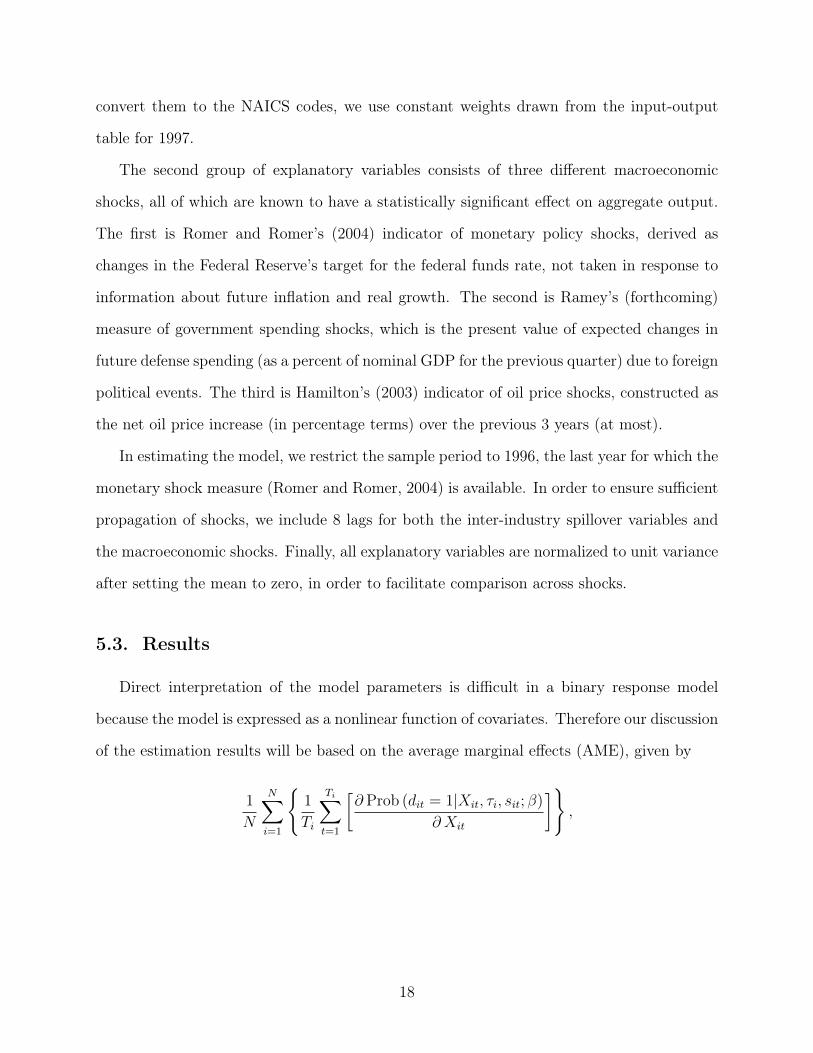
5.3. Results

Direct interpretation of the model parameters is difficult in a binary response model

because the model is expressed as a nonlinear function of covariates. Therefore our discussion

of the estimation results will be based on the average marginal effects (AME), given by

1

N

N∑i=1

{1

Ti

Ti∑t=1

[∂ Prob (dit = 1|Xit, τi, sit; β)

∂ Xit

]},

18

where Ti is the size of the effective sample in which sit = 0 (not censored) for given i.23 The

detailed maximum likelihood estimates of the model parameters are provided in Table A1.

Using these estimates, Figure 7 plots the cumulative impacts of a one-standard-deviation

increase in the explanatory variables, together with the 68% and 95% confidence bands.24

Panel A exhibits the upstream spillover effects for the occurrences of peaks and troughs.

Looking at peaks, in response to a one-standard-deviation increase in the fraction of upstream

industries (output users) that experienced a peak in the previous quarter, the probability of

an industry experiencing a peak increases by 2%. The cumulative effects of this upstream

spillover effect continue to rise for seven quarters, suggesting a gradual but strong upstream

propagation through the input-output linkages. For troughs, the upstream spillover effect

becomes statistically positive only with a two quarters delay, and then begins to fade out

after four quarters.

Panel B shows that the downstream spillover effect is also significant. Having more

downstream industries (input suppliers) experiencing phase shifts also increases the indus-

try’s probability of experiencing a phase shift. In peaks, both upstream and downstream

effects are significant and in similar magnitudes. For troughs, unlike the upstream effect, the

downstream effect is not only immediately significant but also gradually strengthens over

time, reaching its maximum effect after seven quarters. Overall, in troughs, the downstream

effect seems stronger than the upstream effect.

Panel C plots the cumulative effects of monetary policy shocks, identified by Romer

and Romer (2004). Consistent with the prediction from the standard monetary models, an

exogenous increase in the federal funds rate increases the probability of a peak (the end of

expansion) and decreases the probability of a trough (the end of contraction). Of importance

is its asymmetric effect between peaks and troughs. For peaks, a one-standard-deviation23For example, the marginal effect of the kth explanatory variable on the probability of i industry’s

experiencing a phase shift at time t is calculated as βkφ (X ′itβ + τi), where βk is the coefficient on the kthexplanatory variable and φ(·) is the standard normal density.

24Because no lags of the dependent variable are included in the model, the cumulative effect after mquarters is just the sum of the coefficients on the first m lags of the explanatory variables.

19

increase in the federal funds rate increases the probability of an industry experiencing a

peak by 0.6% in the first quarter. While the probability of a peak slightly increases during

the following two quarters, such responses are mostly small and statistically insignificant.

In contrast, the probability of a trough exhibits rapid, persistent, and large declines after a

rise in the federal funds rate. The cumulative impact is between -6.6% and -9.2% for the

first four quarters, and then declines again, reaching -17.5% at the seventh quarter. The

estimated impact is consistently significant even at the 95% confidence level. According to

these results, monetary policy is highly effective in recessions: a decrease in the federal funds

rate increases the probability of exiting a recession significantly. This asymmetric pattern

is consistent with the view that the effect of monetary policy on output growth is greater in

recessions than in expansions; e.g., Weise (1999), Lo and Piger (2005), and Peersman and

Smets (2005).

Government policy shocks, measured by Ramey (forthcoming), have significant effects

on both peaks and troughs (Panel D). Their effects are also somewhat asymmetric. An

exogenous increase in government spending reduces the probability of a peak (the end of

expansion). The cumulative effect reaches -7.0% in the fifth quarter, and then returns toward

zero. For troughs, increased government spending significantly increases the probability of

exiting a contraction phase, with the maximum effect being estimated at 14.9% in the fourth

quarter. Hence, the effect of government spending on the occurrence of a phase shift in

recessions is almost twice as large as that in expansions. This result is consistent with the

recent theoretical (Christiano, Eichenbaum and Rebelo, 2009; Woodford, forthcoming) and

empirical (Auerbach and Gorodnichenko, 2010; Bachmann and Sims, 2011) work that finds

a larger government spending multiplier in recessions using aggregate-level time-series data.

Finally, Panel E shows that oil price shocks, measured by Hamilton (2003), are also

important determinants for industry phase shifts. A one-standard-deviation increase in oil

price raises the propensity of a transition from expansion to contraction, with its maximum

effect being 7.6% in the fourth quarter. The same magnitude of change in oil price lowers

20

the probability of exiting a recession with its maximum effect of -15.8% in the third quarter

after.25

In sum, both the input-output linkages and the three macroeconomic shocks we consider

are important determinants of industrial phase shifts over the business cycle. All of them

are statistically significant and conform with our economic priors. Moreover, they show

interesting asymmetry between peaks and troughs. In particular, both monetary and fiscal

policy shocks are more effective during recessions.

5.4. Robustness

In this subsection we examine whether our conclusions are robust to alternative data and

model specifications. The results are summarized in Figure 8. In our baseline estimation, we

use Hamilton’s (2003) measure of oil price shocks, which is constructed in nominal terms and

does not distinguish underlying causes of the oil price changes. We re-estimate the probit

model using Kilian’s (2008) measure of oil price shocks that captures real oil price changes

driven solely by supply-side disruptions in the crude oil market.26 Our results are generally

robust to this alternative measure of oil price shocks. One notable exception is the effect of

government spending shocks on the occurrence of a trough: it is much weaker with Kilian’s

measure.

We also estimate the model using data disaggregated at the 3-digit NAICS level.27 The

use of 3-digit data yields somewhat imprecise estimates with respect to both spillover effects,

as the number of observations decreases. However, interestingly, the effects of macroeconomic

shocks are much more pronounced, perhaps because they are aggregate common shocks. In25Our results for the effects of oil price shocks do not necessarily conflict with the conventional view that

an oil price increase has a larger output effect than an oil price decrease; Hamilton (2003) and referencestherein. The reason is clear because an asymmetry related to the direction of an oil price change does notimply nor is it implied by an asymmetry related to the responses of peaks and troughs to a given change inoil price.

26We obtain the real oil price shocks as the regression residuals of the growth rate of the real oil price onthe contemporaneous and up to four lags of exogenous oil supply changes documented by Kilian (2008). Thereal price of oil is obtained by deflating the price of crude oil based on the price index for GDP.

27The results of using the 6-digit industry-level data are virtually identical to those reported for the 4-digitindustries.

21

particular, the use of 3-digit data considerably increases the effects of government spending

shocks on the occurrence of a trough. To check whether applying a detrending method would

yield different results, we also estimate the model using the 4-digit data detrended by the

Hodrick-Prescott filter. The results are quite robust even to this alternative choice.

In our baseline model of random effects we implicitly assume that industry-specific factors

do not affect the probabilities of phase shifts. This assumption might be too restrictive. To

address this problem, we allow industry-specific disturbances, denoted as εit in equation

(7), to follow a stationary first-order autoregressive (AR(1)) process.28 As is clear in the

figure, the results are fairly robust to this generalization. We also consider a fixed effects

specification to take into account the possibility that the mean durations of expansion phases

of industries, which are closely related to their trend growth rates (Harding and Pagan,

2002), may not be independent from the explanatory variables, which account for cyclical

movements of industries.29 To correct the bias due to the incidental parameters problem, we

estimate the fixed effects model using the penalized-likelihood-based approximation proposed

by Bester and Hansen (2009). Again, the results are very similar to those of the random

effects model.

Finally, to check the robustness of our results to structural changes in the input-output

linkages during the sample period, we use the 1977 input-output table that is broken down

by the SIC codes. In addition, in order to match this input-output table with IP data, we

also make use of the vintage IP data disaggregated by the same SIC codes.30 Despite large

time gaps between the two input-output tables, the results do not alter significantly. This

evidence is consistent with Carvalho (2010), Holly and Petrella (2010), and Foerster, Sarte

and Watson (forthcoming), who find that the observed changes in the structure of input-

output relations do not seem to substantially distort the effects of the sources of industry28We estimate the model using the Geweke-Hajivassiliou-Keane (GHK) simulator; Lee (1997) for details

of the procedure.29We note that there is a long-standing debate in economics regarding the relationship between long-term

trends and short-term fluctuations in economic variables.30The vintage IP data are constructed by Foerster, Sarte and Watson (forthcoming), and available from

Mark Watson’s website. We use the vintage IP data disaggregated into 84 industries.

22

comovement.

6. Summary

The phase shift carries far richer information about the nature of business cycles than a

simple correlation. In particular, the timing of turning points is of great interest to policy

makers, financial analysts, and individual investors. Based on the IP indices of 74 U.S. man-

ufacturing industries, we identify the turning points of industry cycles using a nonparametric

method developed by Harding and Pagan (2002).

We uncover new empirical regularities about the inter-industry comovement of turning

points that will help us to better understand the nature of business cycles. First, manufac-

turing industries on average have experienced more cycles than the U.S. aggregate economy.

Second, the comovement across industries appears to be a salient feature of manufacturing

business cycles. Third and most important, there is substantial asymmetry in the distri-

bution of turning points between peaks and troughs. Troughs (upturns) are much more

concentrated than peaks (downturns). Occurrences of phase shifts across industries strongly

support the spillovers through input-output linkages, a core aspect of multi-sector models.

We confirm that the standard macroeconomic shocks, such as exogenous changes in the

federal funds rate, defense spending, and oil prices, are important determinants of cyclical

turning points. Their effects on industry phase shifts are all statistically significant and con-

form with our economic priors. Finally, we find that both monetary and fiscal policy shocks

are much more effective in recessions than in expansions.

23

References

Auerbach, Alan J., and Yuriy Gorodnichenko. 2010. “Measuring the Output Responsesto Fiscal Policy.” National Bureau of Economic Research Working Paper 16311.

Bachmann, Ruediger, and Christian Bayer. 2009. “The Cross-Section of Firms overthe Business Cycle: New Facts and a DSGE Exploration.” www-personal.umich.edu/~rudib/bachmann_sims_conf_policy_jan10_11.pdf.

Bachmann, Ruediger, and Eric R. Sims. 2011. “Confidence and the Transmission ofGovernment Spending Shocks.” www-personal.umich.edu/~rudib/bachmann_bayer_

XsectDyn_submittedJPE.pdf.

Bartelsman, Eric J., Ricardo J. Caballero, and Richard K. Lyons. 1994. “Customer-and Supplier-Driven Externalities.” American Economic Review, 84(4): 1075–84.

Bester, C. Alan, and Christian Hansen. 2009. “A Penalty Function Approach to BiasReduction in Nonlinear Panel Models with Fixed Effects.” Journal of Business & Eco-nomic Statistics, 27(2): 131–48.

Bloom, Nocholas, Max Floetotto, and Nir Jaimovich. 2010. “Really Uncertain Busi-ness Cycles.” www.stanford.edu/~nbloom/RUBC_DRAFT.pdf.

Bry, Gerhard, and Charlotte Boschan. 1971. Cyclical Analysis of Time Series: SelectedProcedures and Computer Programs. New York: National Bureau of Economic Research.

Burns, Arthur F., and Wesley C. Mitchell. 1946. Measuring Business Cycles. NewYork: National Bureau of Economic Research.

Butler, J.S., and Robert Moffitt. 1982. “A Computationally Efficient Quadrature Pro-cedure for the One-Factor Multinomial Probit Model.” Econometrica, 50(3): 761–4.

Canova, Fabio. 1998. “Detrending and Business Cycle Facts.” Journal of Monetary Eco-nomics, 41(3): 475–512.

Carvalho, Vasco M. 2010. “Aggregate Fluctuations and the Network Structure of Inter-sectoral Trade.” www.crei.cat/people/carvalho/carvalho_aggregate.pdf.

Christiano, Lawrence J., and Terry J. Fitzgerald. 1998. “The Business Cycle: It’sStill a Puzzle.” Federal Reserve Bank of Chicago Economic Perspective, 22(4): 56–83.

24

Christiano, Lawrence, Martin Eichenbaum, and Sergio Rebelo. 2009. “When Isthe Government Spending Multiplier Large?” National Bureau of Economic ResearchWorking Paper 15394.

Cogley, Timothy, and James M. Nason. 1995. “Effects of the Hodrick-Prescott Filter onTrend and Difference Stationary Time Series: Implications for Business Cycle Research.”Journal of Economic Dynamics and Control, 19(1–2): 253–78.

Conley, Timothy G., and Bill Dupor. 2003. “A Spatial Analysis of Sectoral Comple-mentarity.” Journal of Political Economy, 111(2): 311–52.

Cooper, Russell, and John Haltiwanger. 1990. “Inventories and the Propagation ofSectoral Shocks.” American Economic Review, 80(1): 170–90.

Dupor, Bill. 1999. “Aggregation and Irrelevance in Multi-Sector Models.” Journal of Mon-etary Economics, 43(2): 391–409.

Eichengreen, Barry J., Andrew K. Rose, and Charles Wyplosz. 1996. “ContagiousCurrency Crises: First Tests.” Scandinavian Journal of Economics, 98(4): 463–84.

Eisfeldt, Andrea L., and Adriano A Rampini. 2006. “Capital Reallocation and Liquid-ity.” Journal of Monetary Economics, 53(3): 369–99.

Estrella, Arturo, and Frederic S. Mishkin. 1998. “Predicting U.S. Recessions: FinancialVariables as Leading Indicators.” Review of Economics and Statistics, 80(1): 45–61.

Foerster, Andrew T., Pierre-Daniel G. Sarte, and Mark W. Watson. Forthcoming.“Sectoral vs. Aggregate Shocks: A Structural Factor Analysis of Industrial Production.”Journal of Political Economy.

Goolsbee, Austan, and Peter J. Klenow. 2002. “Evidence on Learning and NetworkExternalities in the Diffusion of Home Computers.” Journal of Law and Economics,45(2): 317–43.

Hamilton, James D. 2003. “What is an Oil Shock?” Journal of Econometrics, 113(2): 363–98.

Harding, Don, and Adrian R. Pagan. 2002. “Dissecting the Cycle: A MethodologicalInvestigation.” Journal of Monetary Economics, 49(2): 365–81.

Harding, Don, and Adrian R. Pagan. 2006. “Synchronization of Cycles.” Journal ofEconometrics, 132(1): 59–79.

25

Harding, Don, and Adrian R. Pagan. 2011. “An Econometric Analysis of Some Mod-els for Constructed Binary Time Series.” Journal of Business & Economic Statistics,29(1): 86–95.

Harvey, Andrew C., and A. Jaeger. 1993. “Detrending, Stylized Facts and the BusinessCycle.” Journal of Applied Econometrics, 8(3): 231–47.

Hess, Gregory D., and Shigeru Iwata. 1997. “Measuring and Comparing Business-CycleFeatures.” Journal of Business & Economic Statistics, 15(4): 432–44.

Hicks, John R. 1950. A Contribution to the Theory of the Trade Cycle. Oxford: ClarendonPress.

Higgins, James J. 2004. Introduction to Nonparametric Statistics. Pacific Grove, CA:Brooks/Cole.

Higson, Chris, Sean Holly, and Paul Kattuman. 2002. “The Cross-Sectional Dynamicsof the US Business Cycle: 1950–1999.” Journal of Economic Dynamics and Control,26(9–10): 1539–55.

Hodrick, Robert J., and Edward C. Prescott. 1997. “Postwar U.S. Business Cycles:An Empirical Investigation.” Journal of Money, Credit and Banking, 29(1): 1–16.

Holly, Sean, and Ivan Petrella. 2010. “Factor Demand Linkages, Technology Shocks andthe Business Cycle.” www.ivanpetrella.com/research.

Hornstein, Andreas. 2000. “The Business Cycle and Industry Comovement.” Federal Re-serve Bank of Richmond Economic Quarterly, 86(4): 27–48.

Hornstein, Andreas, and Jack Praschnik. 1997. “Intermediate Inputs and SectoralComovement in the Business Cycle.” Journal of Monetary Economics, 40(3): 573–95.

Horvath, Michael. 2000. “Sectoral Shocks and Aggregate Fluctuations.” Journal of Mon-etary Economics, 45(1): 69–106.

Kehrig, Matthias. 2011. “The Cyclicality of Productivity Dispersion.” www.depot.

northwestern.edu/~mke816/Kehrig_jmp.pdf.

Keynes, John M. 1936. The General Theory of Employment, Interest and Money. London:Macmillan.

26

Kilian, Lutz. 2008. “Exogenous Oil Supply Shocks: How Big Are They and How Much DoThey Matter for the U.S. Economy?” Review of Economics and Statistics, 90(2): 216–40.

Kim, Young Sik, and Kunhong Kim. 2006. “How Important is the Intermediate InputChannel in Explaining Sectoral Employment Comovement over the Business Cycle?”Review of Economic Dynamics, 9(4): 659–82.

King, Robert, and Charles I Plosser. 1994. “Real Business Cycles and the Test of theAdelmans.” Journal of Monetary Economics, 33(2): 405–38.

Kydland, Finn E., and Edward C. Prescott. 1990. “Business Cycles: Real Facts and aMonetary Myth.” Federal Reserve Bank of Minneapolis Quarterly Review, 14(1): 3–18.

Lee, Lung-Fei. 1997. “Simulated Maximum Likelihood Estimation of Dynamic DiscreteChoice Statistical Models: Some Monte Carlo Results.” Journal of Econometrics,82(1): 1–35.

Lo, Ming C., and Jeremy M. Piger. 2005. “Is the Response of Output to MonetaryPolicy Asymmetric? Evidence from a Regime-Switching Coefficients Model.” Journalof Money, Credit, and Banking, 37(5): 865–86.

Long, John B., Jr., and Charles I. Plosser. 1983. “Real Business Cycles.” Journal ofPolitical Economy, 91(1): 39–69.

Long, John B., Jr., and Charles I. Plosser. 1987. “Sectoral vs. Aggregate Shocks in theBusiness Cycle.” American Economic Review, 77(2): 333–6.

Lucas, Robert E., Jr. 1977. “Understanding Business Cycles.” Carnegie-Rochester Con-ference Series on Public Policy, 5: 7–29.

McQueen, Grant, and Steven Thorley. 1993. “Asymmetric Business Cycle TurningPoints.” Journal of Monetary Economics, 31(3): 341–62.

Morley, James C. 2009. “Macroeconomics, Nonlinear Time Series.” In Encyclopedia ofComplexity and Systems Science, ed. Robert A. Meyers, 5325–48. Berlin: Springer.

Murphy, Kevin M., Andrei Shleifer, and Robert W. Vishny. 1989. “Building Blocksof Market Clearing Business Cycle Models.” In NBER Macroeconomics Annual 1989,Volume 4, ed. Olivier Jean Blanchard and Stanley Fischer, 247–302. Cambridge, MA:MIT Press.

27

Padian, Nancy S., Stephen C. Shiboski, Sarah O. Glass, and Eric Vittinghoff.1997. “Heterosexual Transmission of Human Immunodeficiency Virus (HIV) in North-ern California: Results from a Ten-year Study.” American Journal of Epidemiology,146(4): 350–7.

Peersman, Gert, and Frank Smets. 2005. “The Industry Effects of Monetary Policy inthe Euro Area.” Economic Journal, 115(503): 319–42.

Ramey, Valerie A. Forthcoming. “Identifying Government Spending Shocks: It’s All inthe Timing.” Quarterly Journal of Economics.

Romer, Christina D., and David H. Romer. 2004. “A New Measure of MonetaryShocks: Derivation and Implications.” American Economic Review, 94(4): 1055–84.

Shea, John S. 2002. “Complementarities and Comovements.” Journal of Money, Credit,and Banking, 34(2): 412–33.

Veldkamp, Laura, and Justin Wolfers. 2007. “Aggregate Shocks or Aggregate Infor-mation? Costly Information and Business Cycle Comovement.” Journal of MonetaryEconomics, 54(1): 37–55.

Watson, Mark W. 1994. “Business Cycle Durations and Postwar Stabilization of the U.S.Economy.” American Economic Review, 84(1): 24–46.

Weise, Charles L. 1999. “The Asymmetric Effects of Monetary Policy: A Nonlinear VectorAutoregression Approach.” Journal of Money, Credit and Banking, 31(1): 85–108.

Woodford, Michael. Forthcoming. “Simple Analytics of the Government Expenditure Mul-tiplier.” American Economic Journal: Macroeconomics.

28

Table 1. Industry Cycles, 1972:Q1–2010:Q2

Duration

No. ofcycles

Completecycle

Expansion(A)

Contraction(B)

Durationasymmetry

(A/B)

NBER cycle 5.0 27.4 23.8 3.8 6.2

Industry cyclesMean 10.3 14.2 8.7 5.3 1.8Median 10.0 13.5 7.6 5.1 1.5Max 16.0 34.0 31.3 8.9 10.4Min 4.0 8.3 3.8 2.6 0.5Std. 2.5 4.5 4.3 1.3 1.5

Note: Complete cycles are measured from trough to trough.

Table 2. Concordance Indices

Pairwise NBER

Mean 0.607 0.674Median 0.604 0.669Max 0.864 0.883Min 0.344 0.455Std. 0.080 0.082

Note: ‘Pairwise’ measures the concordance between industries.‘NBER’ measures the concordance of industries with the aggre-gate U.S. economy whose turning points are determined by theNBER.

29

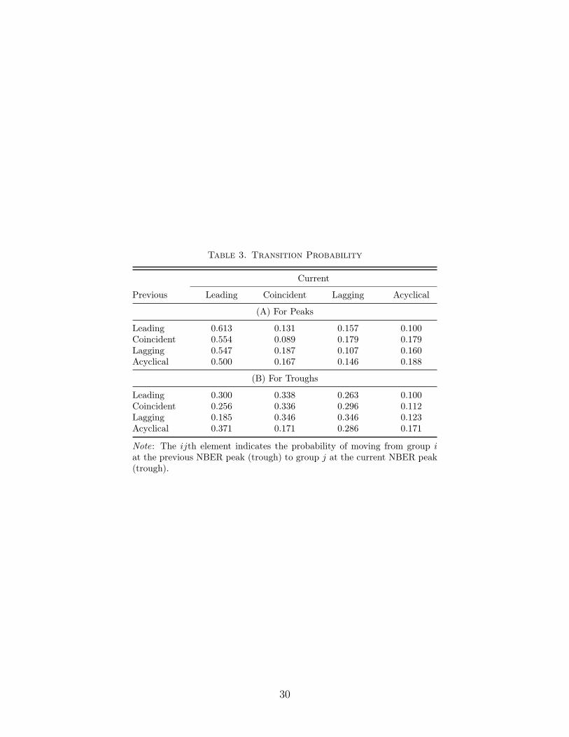
Table 3. Transition Probability

Current

Previous Leading Coincident Lagging Acyclical

(A) For Peaks

Leading 0.613 0.131 0.157 0.100Coincident 0.554 0.089 0.179 0.179Lagging 0.547 0.187 0.107 0.160Acyclical 0.500 0.167 0.146 0.188

(B) For Troughs

Leading 0.300 0.338 0.263 0.100Coincident 0.256 0.336 0.296 0.112Lagging 0.185 0.346 0.346 0.123Acyclical 0.371 0.171 0.286 0.171

Note: The ijth element indicates the probability of moving from group iat the previous NBER peak (trough) to group j at the current NBER peak(trough).

30

Table 4. Leading, Coincident, and Lagging Industries at the NBER Peak Dates

Code Dur. Industry title Prob. Leads (-) or lags (+)

Mean Std.

Leading industries3322 D Cutlery and handtool 1.00 -3.00 1.413361 D Motor vehicle 1.00 -3.00 1.793371 D Furniture and kitchen cabinet 1.00 -1.83 1.173325 D Hardware 0.83 -4.40 2.073362 D Motor vehicle body and trailer 0.83 -4.40 2.703255 ND Paint, coating, and adhesive 0.83 -3.80 2.683212 D Veneer, plywood, and engineered wood product 0.83 -3.60 2.073219 D Other wood product 0.83 -3.40 1.953221 ND Pulp, paper, and paperboard mills 0.83 -3.40 2.303352 D Household appliance 0.83 -3.00 2.353274 D Lime and gypsum product 0.83 -3.00 2.923252 ND Resin, synth. rubber, fibers, and filaments 0.83 -2.80 1.643253 ND Pestic., fertil., and agric. chemical 0.83 -2.60 2.073351 D Electric lighting equipment 0.83 -2.40 1.343372A9 D Office and other furniture 0.83 -2.20 1.303315 D Foundries 0.67 -4.75 2.873211 D Sawmills and wood preservation 0.67 -4.50 2.083363 D Motor vehicle parts 0.67 -4.50 2.083122 ND Tobacco 0.67 -4.25 3.773334 D Ventilat., heat., air-cond., and refrig. equip. 0.67 -4.00 2.163149 ND Other textile product mills 0.67 -4.00 2.453118 ND Bakeries and tortilla 0.67 -4.00 2.943133 ND Textile and fabr. finishing and fabr. coating mills 0.67 -3.75 1.263343 D Audio and video equipment 0.67 -3.75 1.713131 ND Fiber, yarn, and thread mills 0.67 -3.75 2.363353 D Electrical equipment 0.67 -3.75 2.363273 D Cement and concrete product 0.67 -3.25 1.503329 D Other fabricated metal product 0.67 -3.25 3.303279 D Other nonmetallic mineral product 0.67 -3.00 2.123141 ND Textile furnishings mills 0.67 -2.25 0.50Lagging industries3113 ND Sugar and confectionery product 0.67 1.50 1.003345 D Navig., measur., electromed., and contr. instr. 0.67 2.50 1.29

Note: ‘D’ and ‘ND’ stand for durables and nondurables, respectively. ‘Prob.’ denotes the unconditionalprobability of being classified in a group at a NBER peak. ‘Mean’ and ‘Std.’ are the conditional mean andstandard deviation of leads or lags at the NBER peaks, given that the industry belongs to the specifiedgroup.

31

Table 5. Leading, Coincident, and Lagging Industries at the NBER Trough Dates

Code Dur. Industry title Prob. Leads (-) or lags (+)

Mean Std.

Leading industries3391 D Medical equipment and supplies 0.67 -3.50 3.323113 ND Sugar and confectionery product 0.67 -3.20 2.283211 D Sawmills and wood preservation 0.67 -3.00 2.45Coincident industries3149 ND Other textile product mills 0.83 0.00 0.003325 D Hardware 0.83 0.00 0.003311A2 D Iron and steel products 0.83 0.00 0.003132 ND Fabric mills 0.67 0.00 0.003133 ND Textile and fabr. finishing and fabr. coating mills 0.67 0.00 0.003327 D Machine shop; screw, nut, and bolt 0.67 0.00 0.003371 D Furniture and kitchen cabinet 0.67 0.00 0.003261 ND Plastics product 0.67 0.00 0.003272 D Glass and glass product 0.67 0.00 0.003315 D Foundries 0.67 0.00 0.00Lagging industries3333A9 D Commercial and service industry machinery 0.83 1.80 1.303336 D Engine, turbine, and power trans. equipment 0.83 2.40 2.613118 ND Bakeries and tortilla 0.83 2.40 2.613353 D Electrical equipment 0.83 2.80 2.393256 ND Soap, cleaning compound, and toilet preparation 0.83 3.00 2.553345 D Navig., measur., electromed., and contr. instr. 0.67 2.25 1.503321 D Forging and stamping 0.67 2.75 0.963331 D Agriculture, construction, and mining machinery 0.67 2.75 2.063122 ND Tobacco 0.67 3.00 1.413111 ND Animal food 0.67 3.00 1.413335 D Metalworking machinery 0.67 3.20 2.773365 D Railroad rolling stock 0.67 4.50 2.38

Note: See footnote of Table 4.

32

Table 6. Sharpness Asymmetry for Each Group of Industries

Peaks Troughs Sharpness asymmetry

DP,−2 DP,+2 SP DT,−2 DT,+2 ST (ST − SP )

Total -0.003 -0.046 0.062 -0.077 0.038 0.126 0.065∗Coincident 0.034 -0.063 0.097 -0.120 0.089 0.209 0.112∗Others -0.009 -0.043 0.056 -0.056 0.012 0.085 0.029∗

Leading -0.029 -0.068 0.059 -0.020 0.055 0.096 0.037∗Lagging 0.034 0.013 0.049 -0.083 -0.018 0.083 0.035∗Acyclical 0.003 -0.031 0.056 -0.035 0.024 0.070 0.013

Note: For peaks, DP,−2 and DP,+2 indicate the mean changes in the log IP during the two quarters ending inthe NBER peak dates and those during the two quarters following the NBER peak dates. SP measures themean sharpness of the log IP at the NBER peak date, defined as the absolute difference between DP,−2 andDP,+2. For troughs, DT,−2, DT,+2, and ST are defined in a similar way. Sharpness asymmetry is measuredby the difference between ST and SP . Asterisk indicates that the Welch t-test rejects the null of no sharpnessasymmetry at the 5% level or less.

Table 7. Decomposition of Sharpness Asymmetry

NBER recessions ST − SP Composition effect (%) Individual asymmetry (%)

1973–75 0.151 0.030 (19.5) 0.122 (80.5)1980 0.045 0.010 (22.5) 0.035 (77.5)1981–82 0.028 0.003 (9.2) 0.026 (90.8)1990–91 0.029 0.014 (48.5) 0.015 (51.5)2001 0.022 0.017 (74.6) 0.006 (25.4)2007–09 0.112 0.022 (19.3) 0.090 (80.7)

Mean 0.065 0.016 (24.3) 0.049 (75.7)

Note: The second column shows sharpness asymmetry at the aggregate level, estimated for each NBERrecession. ‘Composition effect’ corresponds to the sharpness asymmetry due to changes in the fraction ofcoincident and other industries. ‘Individual asymmetry’ corresponds to the sharpness asymmetry attributedto the changes in sharpness for each group of industries between NBER troughs and peaks. The values inparentheses are the share of sharpness asymmetry (in percentage terms) explained by each source.

33

Table A.1. Maximum Likelihood Estimates of Models for Industry Phase Shifts

Variable Peak equation Trough equation

Lag Index coefficient AME Index coefficient AME

Upstream spillovert− 1 0.105∗ (0.030) 0.021∗ (0.007) 0.010 (0.040) 0.003 (0.012)t− 2 0.036 (0.034) 0.007 (0.007) 0.178∗ (0.045) 0.049∗ (0.013)t− 3 0.022 (0.036) 0.004 (0.008) 0.000 (0.054) 0.000 (0.016)t− 4 0.039 (0.035) 0.008 (0.008) 0.012 (0.056) 0.003 (0.017)t− 5 0.025 (0.033) 0.005 (0.007) -0.098 (0.051) -0.027 (0.015)t− 6 0.061 (0.033) 0.012 (0.007) -0.062 (0.042) -0.017 (0.013)t− 7 0.015 (0.034) 0.003 (0.007) -0.031 (0.042) -0.009 (0.013)t− 8 -0.044 (0.036) -0.009 (0.008) 0.029 (0.043) 0.008 (0.013)

Downstream spillovert− 1 0.124∗ (0.030) 0.024∗ (0.007) 0.116∗ (0.041) 0.032∗ (0.012)t− 2 0.021 (0.035) 0.004 (0.008) 0.000 (0.048) 0.000 (0.014)t− 3 0.020 (0.037) 0.004 (0.008) 0.047 (0.051) 0.013 (0.015)t− 4 0.040 (0.036) 0.008 (0.008) 0.017 (0.055) 0.005 (0.016)t− 5 -0.010 (0.035) -0.002 (0.008) 0.006 (0.049) 0.002 (0.015)t− 6 -0.061 (0.036) -0.012 (0.008) 0.099∗ (0.045) 0.027∗ (0.013)t− 7 0.023 (0.034) 0.004 (0.007) 0.004 (0.047) 0.001 (0.014)t− 8 -0.033 (0.037) -0.007 (0.008) -0.137∗ (0.051) -0.038∗ (0.015)

Monetary policy shockt− 1 0.029 (0.041) 0.006 (0.009) -0.272∗ (0.041) -0.075∗ (0.011)t− 2 0.067 (0.041) 0.013 (0.009) 0.033 (0.054) 0.009 (0.016)t− 3 0.024 (0.041) 0.005 (0.009) -0.094 (0.051) -0.026 (0.015)t− 4 -0.101∗ (0.044) -0.020∗ (0.010) 0.065 (0.054) 0.018 (0.016)t− 5 0.014 (0.047) 0.003 (0.010) -0.283∗ (0.054) -0.078∗ (0.016)t− 6 0.033 (0.048) 0.006 (0.010) -0.083 (0.048) -0.023 (0.014)t− 7 0.165∗ (0.048) 0.033∗ (0.011) 0.001 (0.047) 0.000 (0.014)t− 8 -0.004 (0.041) -0.001 (0.009) 0.183∗ (0.047) 0.051∗ (0.014)

Government spending shockt− 1 -0.114∗ (0.036) -0.023∗ (0.008) 0.368∗ (0.054) 0.102∗ (0.017)t− 2 -0.098∗ (0.032) -0.019∗ (0.007) 0.075∗ (0.038) 0.021 (0.011)t− 3 -0.084∗ (0.035) -0.017∗ (0.008) 0.087 (0.045) 0.024 (0.014)t− 4 -0.015 (0.039) -0.003 (0.009) 0.009 (0.038) 0.003 (0.011)t− 5 -0.044 (0.041) -0.009 (0.009) -0.028 (0.041) -0.008 (0.012)t− 6 0.119∗ (0.044) 0.023∗ (0.010) -0.220∗ (0.043) -0.061∗ (0.013)t− 7 0.056 (0.045) 0.011 (0.010) -0.054 (0.044) -0.015 (0.013)t− 8 0.055 (0.054) 0.011 (0.012) 0.053 (0.047) 0.015 (0.014)

Oil price shockt− 1 0.020 (0.039) 0.004 (0.009) -0.063 (0.054) -0.017 (0.016)t− 2 0.267∗ (0.047) 0.053∗ (0.010) -0.206∗ (0.063) -0.057∗ (0.019)t− 3 0.092 (0.061) 0.018 (0.013) -0.289∗ (0.054) -0.080∗ (0.017)t− 4 0.006 (0.075) 0.001 (0.016) -0.014 (0.035) -0.004 (0.011)t− 5 -0.004 (0.053) -0.001 (0.011) 0.140∗ (0.040) 0.039∗ (0.012)t− 6 -0.100∗ (0.045) -0.020 (0.010) 0.099 (0.052) 0.028 (0.015)t− 7 -0.039 (0.037) -0.008 (0.008) -0.032 (0.056) -0.009 (0.017)t− 8 -0.085∗ (0.037) -0.017∗ (0.008) 0.104 (0.055) 0.029 (0.016)

Constant -1.108∗ (0.044) -0.706∗ (0.047)στ 0.257∗ (0.042) 0.208∗ (0.051)lnL -1277.8 -950.1No. obs. 3588 1935

Notes: The estimated model is given by equations (6) and (7). Index coefficients are the model parameters.AME is the abbreviation for “Average Marginal Effect.” The values in parentheses are asymptotic standarderrors. The asymptotic standard errors of index coefficients are obtained from the inverse of the Hessianat the maximum likelihood estimates, and those of AMEs are computed using the delta method. Asteriskindicates significance at 5% level or less.

34

Figure 1. U.S. Log Real GDP and Business Cycle Dates: NBER vs Hard-ing and Pagan

7.2

7.6

8.0

8.4

8.8

9.2

9.6

50 55 60 65 70 75 80 85 90 95 00 05 10

PT PT PT PT PT PT PTPT PT PT

Note: ‘P’ and ‘T’ correspond to the peaks and troughs identified by the Harding-Paganmethod applied to the log level of U.S. real GDP. The shaded areas are recession periodsestablished by the NBER.

35

Figure 2. Diffusion Indices for Cyclical Phases

1975 1980 1985 1990 1995 2000 2005 2010

equal weights output share weights

Contraction

1975 1980 1985 1990 1995 2000 2005 2010

equal weights output share weights

Expansion

1.0

0.5

0.0

1.0

0.5

0.0

36

Figure 3. Distributions of Industry Turning Points, 1972:Q1–2010:Q2

0.00

0.05

0.10

0.15

0.20

0.25

0.30

0.35

-8 -7 -6 -5 -4 -3 -2 -1 0 1 2 3 4 5 6 7 8

Frac

tion

of in

dust

ries

Leads (-) or lags (+) at the NBER dates

peak trough

37

Figure 4. Distributions of Industry Turning Points for Each NBER Recession

0.000.050.100.150.200.250.300.350.400.45

-8 -7 -6 -5 -4 -3 -2 -1 0 1 2 3 4 5 6 7 8

1973-75 Recession

peaktrough

0.000.050.100.150.200.250.300.350.400.45

-8 -7 -6 -5 -4 -3 -2 -1 0 1 2 3 4 5 6 7 8

1980 Recession

peaktrough

0.000.050.100.150.200.250.300.350.400.45

-8 -7 -6 -5 -4 -3 -2 -1 0 1 2 3 4 5 6 7 8

1981-82 Recession

peaktrough

0.000.050.100.150.200.250.300.350.400.45

-8 -7 -6 -5 -4 -3 -2 -1 0 1 2 3 4 5 6 7 8

1990-91 Recession

peaktrough

0.000.050.100.150.200.250.300.350.400.45

-8 -7 -6 -5 -4 -3 -2 -1 0 1 2 3 4 5 6 7 8

2001 Recessionpeaktrough

0.000.050.100.150.200.250.300.350.400.45

-8 -7 -6 -5 -4 -3 -2 -1 0 1 2 3 4 5 6 7 8

2007-09 Recessionpeaktrough

Frac

tion

of in

dust

ries

Frac

tion

of in

dust

ries

Frac

tion

of in

dust

ries

Leads (-) or lags (+) at the NBER dates Leads (-) or lags (+) at the NBER dates

38

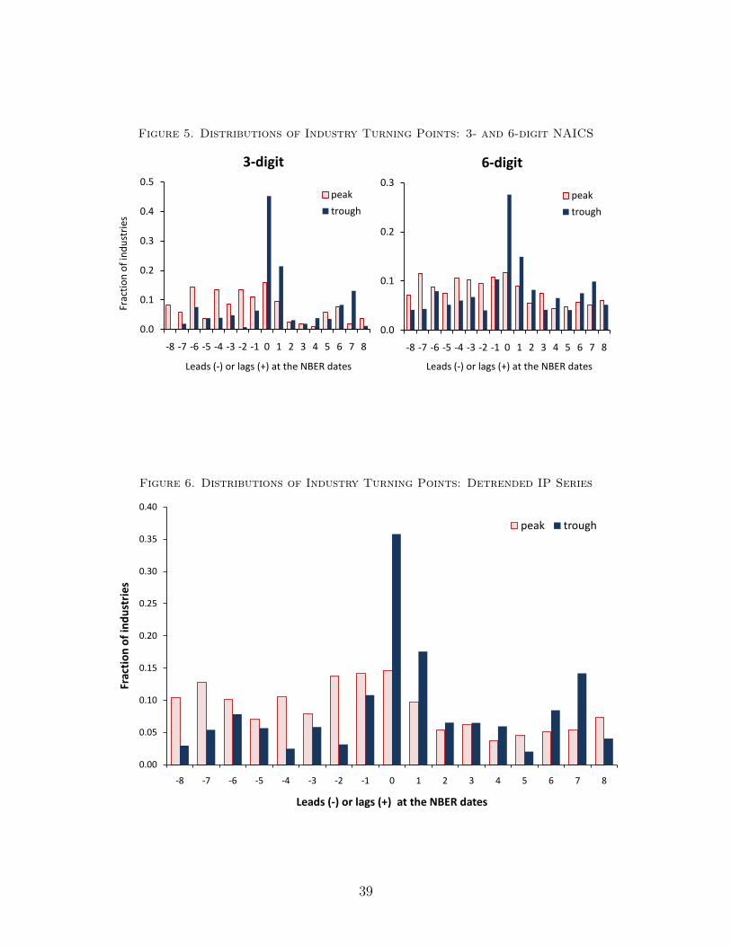
Figure 5. Distributions of Industry Turning Points: 3- and 6-digit NAICSFr

actio

n of

indu

strie

s

Leads (-) or lags (+) at the NBER dates Leads (-) or lags (+) at the NBER dates

0.0

0.1

0.2

0.3

0.4

0.5

-8 -7 -6 -5 -4 -3 -2 -1 0 1 2 3 4 5 6 7 8

3-digit

peaktrough

0.0

0.1

0.2

0.3

-8 -7 -6 -5 -4 -3 -2 -1 0 1 2 3 4 5 6 7 8

6-digit

peaktrough

Figure 6. Distributions of Industry Turning Points: Detrended IP Series

0.00

0.05

0.10

0.15

0.20

0.25

0.30

0.35

0.40

-8 -7 -6 -5 -4 -3 -2 -1 0 1 2 3 4 5 6 7 8

Frac

tion

of in

dust

ries

Leads (-) or lags (+) at the NBER dates

peak trough

39

Figure 7. The Cumulative Marginal Effects of a One-standard-deviation Increasein the Explanatory Variables on the Probabilities of Industry PhaseShifts

(with 68% (dashed line) and 95% (dotted line) confidence intervals)

A. Upstream spillover

B. Downstream spillover

-0.10

-0.05

0.00

0.05

0.10

0.15

0.20

1 2 3 4 5 6 7 8Pr

obab

ility

Quarter

Trough

-0.10

-0.05

0.00

0.05

0.10

0.15

0.20

1 2 3 4 5 6 7 8

Prob

abili

ty

Quarter

Peak

-0.10

-0.05

0.00

0.05

0.10

0.15

0.20

1 2 3 4 5 6 7 8

Prob

abili

ty

Quarter

Peak

-0.10

-0.05

0.00

0.05

0.10

0.15

0.20

1 2 3 4 5 6 7 8

Prob

abili

ty

Quarter

Trough

A. Upstream spillover

B. Downstream spillover

-0.10

-0.05

0.00

0.05

0.10

0.15

0.20

1 2 3 4 5 6 7 8

Prob

abili

tyQuarter

Trough

-0.10

-0.05

0.00

0.05

0.10

0.15

0.20

1 2 3 4 5 6 7 8

Prob

abili

ty

Quarter

Peak

-0.10

-0.05

0.00

0.05

0.10

0.15

0.20

1 2 3 4 5 6 7 8

Prob

abili

ty

Quarter

Peak

-0.10

-0.05

0.00

0.05

0.10

0.15

0.20

1 2 3 4 5 6 7 8

Prob

abili

ty

Quarter

Trough

C. Monetary policy shock

D. Government spending shock

-0.30 -0.25 -0.20 -0.15 -0.10 -0.05 0.00 0.05 0.10 0.15

1 2 3 4 5 6 7 8

Prob

abili

ty

Quarter

Trough

-0.30 -0.25 -0.20 -0.15 -0.10 -0.05 0.00 0.05 0.10 0.15

1 2 3 4 5 6 7 8

Prob

abili

ty

Quarter

Peak

-0.15

-0.10

-0.05

0.00

0.05

0.10

0.15

0.20

0.25

1 2 3 4 5 6 7 8

Prob

abili

ty

Quarter

Trough

-0.15

-0.10

-0.05

0.00

0.05

0.10

0.15

0.20

0.25

1 2 3 4 5 6 7 8

Prob

abili

ty

Quarter

Peak40

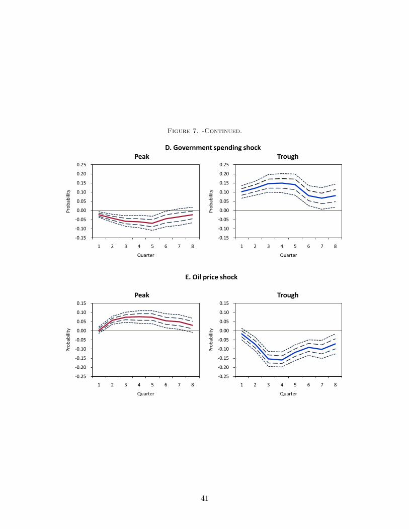
Figure 7. -Continued.

C. Monetary policy shock

D. Government spending shock

-0.30 -0.25 -0.20 -0.15 -0.10 -0.05 0.00 0.05 0.10 0.15

1 2 3 4 5 6 7 8

Prob

abili

ty

Quarter

Trough

-0.30 -0.25 -0.20 -0.15 -0.10 -0.05 0.00 0.05 0.10 0.15

1 2 3 4 5 6 7 8

Prob

abili

ty

Quarter

Peak

-0.15

-0.10

-0.05

0.00

0.05

0.10

0.15

0.20

0.25

1 2 3 4 5 6 7 8

Prob

abili

ty

Quarter

Trough

-0.15

-0.10

-0.05

0.00

0.05

0.10

0.15

0.20

0.25

1 2 3 4 5 6 7 8

Prob

abili

ty

Quarter

Peak

-0.30 -0.25 -0.20 -0.15 -0.10 -0.05 0.00 0.05 0.10 0.15

1 2 3 4 5 6 7 8

Prob

abili

ty

Quarter

Peak

C. Monetary Policy Shock

E. Oil price shock

-0.30 -0.25 -0.20 -0.15 -0.10 -0.05 0.00 0.05 0.10 0.15

1 2 3 4 5 6 7 8

Prob

abili

ty

Quarter

Trough

-0.25

-0.20

-0.15

-0.10

-0.05

0.00

0.05

0.10

0.15

1 2 3 4 5 6 7 8

Prob

abili

ty

Quarter

Peak

-0.25

-0.20

-0.15

-0.10

-0.05

0.00

0.05

0.10

0.15

1 2 3 4 5 6 7 8

Prob

abili

ty

Quarter

Trough

41

Figure 8. Results of Various Sensitivity Exercises

(Baseline model: Hamilton’s oil price shocks, 4-digit classification, Random effectsmodel without idiosyncratic dynamics, 1997 IO table)

A. Upstream spillover

B. Downstream spillover

-0.10

-0.05

0.00

0.05

0.10

0.15

1 2 3 4 5 6 7 8

Prob

abili

ty

Quarter

Peak

-0.10

-0.05

0.00

0.05

0.10

0.15

1 2 3 4 5 6 7 8

Prob

abili

tyQuarter

Trough

-0.10

-0.05

0.00

0.05

0.10

0.15

1 2 3 4 5 6 7 8

Prob

abili

ty

Quarter

Peak

-0.10

-0.05

0.00

0.05

0.10

0.15

1 2 3 4 5 6 7 8

Prob

abili

ty

Quarter

Trough

A. Upstream spillover

B. Downstream spillover

-0.10

-0.05

0.00

0.05

0.10

0.15

1 2 3 4 5 6 7 8

Prob

abili

ty

Quarter

Peak

-0.10

-0.05

0.00

0.05

0.10

0.15

1 2 3 4 5 6 7 8

Prob

abili

ty

Quarter

Trough

-0.10

-0.05

0.00

0.05

0.10

0.15

1 2 3 4 5 6 7 8

Prob

abili

ty

Quarter

Peak

-0.10

-0.05

0.00

0.05

0.10

0.15

1 2 3 4 5 6 7 8

Prob

abili

ty

Quarter

Trough

C. Monetary policy shock

D. Government spending shock

-0.30 -0.25 -0.20 -0.15 -0.10 -0.05 0.00 0.05 0.10 0.15

1 2 3 4 5 6 7 8

Prob

abili

ty

Quarter

Peak

-0.30 -0.25 -0.20 -0.15 -0.10 -0.05 0.00 0.05 0.10 0.15

1 2 3 4 5 6 7 8

Prob

abili

ty

Quarter

Trough

-0.15

-0.10

-0.05

0.00

0.05

0.10

0.15

0.20

0.25

1 2 3 4 5 6 7 8

Prob

abili

ty

Quarter

Peak

-0.15

-0.10

-0.05

0.00

0.05

0.10

0.15

0.20

0.25

1 2 3 4 5 6 7 8

Prob

abili

ty

Quarter

Trough

42

Figure 8. -Continued.

C. Monetary policy shock

D. Government spending shock

-0.30 -0.25 -0.20 -0.15 -0.10 -0.05 0.00 0.05 0.10 0.15

1 2 3 4 5 6 7 8

Prob

abili

ty

Quarter

Peak

-0.30 -0.25 -0.20 -0.15 -0.10 -0.05 0.00 0.05 0.10 0.15

1 2 3 4 5 6 7 8

Prob

abili

ty

Quarter

Trough

-0.15

-0.10

-0.05

0.00

0.05

0.10

0.15

0.20

0.25

1 2 3 4 5 6 7 8

Prob

abili

ty

Quarter

Peak

-0.15

-0.10

-0.05

0.00

0.05

0.10

0.15

0.20

0.25

1 2 3 4 5 6 7 8

Prob

abili

ty

Quarter

Trough

-0.30 -0.25 -0.20 -0.15 -0.10 -0.05 0.00 0.05 0.10 0.15

1 2 3 4 5 6 7 8

Prob

abili

ty

Quarter

Peak

C. Monetary Policy Shock

E. Oil price shock

-0.30 -0.25 -0.20 -0.15 -0.10 -0.05 0.00 0.05 0.10 0.15

1 2 3 4 5 6 7 8

Prob

abili

ty

Quarter

Trough

-0.25 -0.20 -0.15 -0.10 -0.05 0.00 0.05 0.10 0.15 0.20

1 2 3 4 5 6 7 8

Prob

abili

ty

Quarter

Trough

-0.25 -0.20 -0.15 -0.10 -0.05 0.00 0.05 0.10 0.15 0.20

1 2 3 4 5 6 7 8

Prob

abili

ty

Quarter

Peak

-0.10 -0.05 0.00 0.05 0.10 0.15

1 2 3 4 5 6 7 8

obab

ility

Quarter

Trough

baseline Kilian 3-digit Detrended RE+AR(1) FE 1977 IO

43