university of miskolc faculty of mechanical engineering and...
TRANSCRIPT

UNIVERSITY OF MISKOLCFACULTY OF MECHANICAL
ENGINEERING AND INFORMATICS
THESIS WORK
Verification of Performance of InductionMotor Field Oriented Control Strategy
Sam Van NieuwenhuyseKaho Sint-Lieven
AdvisorÁdám Tihamér
Department of Automatization
Miskolc, 2007
"The author and the advisor give the permission to make this thesis available for consul-tation and to copy parts of it for personal use. Every other usage covers the restrictionsof the copyright, in particular with respect to the obligation to mention the source whenquoting results from this thesis."
June 12, 2007
Sam Van Nieuwenhuyse Prof. Dr. Ádám Tihamér
i

Preface
I would like to thank everyone who has contributed to the achievement of this thesis.First of all, I would like to thank my advisor, Prof. Dr. Ádám Tihamér, to offer me theopportunity to perform this kind of research. This thesis has strengthened my interest ofelectric motors. I specially want to thank my advisor for the flexibility he has shown withregard to the subject of my work.Prof. Dr. G. Szeidl deserves a word of thanks for his help with the computer programLatex. I also want to thank Prof. Dr. J. Vásárhelyi to make some time for looking atmy Matlab notes. Furthermore the lab assistant deserves a mention because he shared theinfrastructure with me and showed a lot of patience while helping me with some problems.Also Attila is worth mentioning for his help with some communication problems.Then I continue to say a thank-you to all my friends. They supported me, not only thisyear, but during the whole four-year training. Especially Wouter, also a Belgian Erasmusstudent, made sure that "the Hungarian experience" very pleasant.Without the help of my parents, I would never succeeded in finishing this thesis. Theyhave supported and encouraged me during the last four years. Because of there hard work,I was able to follow the training and spent my last semester in a foreign country.Last, but not least, I want to thank my girlfriend Laurence to have confidence in mycapability and for her support far away in Belgium.
nagyon szépen köszönöm!
ii
Contents
1 Introduction 2
2 The three-phase induction motor (asynchrone motor) 32.1 Introduction . . . . . . . . . . . . . . . . . . . . . . . . . . . . . . . . . . . . 32.2 Construction concept . . . . . . . . . . . . . . . . . . . . . . . . . . . . . . . 3
2.2.1 Stator . . . . . . . . . . . . . . . . . . . . . . . . . . . . . . . . . . . 32.2.2 Rotor . . . . . . . . . . . . . . . . . . . . . . . . . . . . . . . . . . . 4
2.3 Principles, basic formulas . . . . . . . . . . . . . . . . . . . . . . . . . . . . 52.3.1 Principle of operation . . . . . . . . . . . . . . . . . . . . . . . . . . 52.3.2 The rotation field . . . . . . . . . . . . . . . . . . . . . . . . . . . . . 62.3.3 Starting characteristics of a Squirrel-Cage motor . . . . . . . . . . . 82.3.4 Acceleration of the rotor . . . . . . . . . . . . . . . . . . . . . . . . . 82.3.5 Motor under load . . . . . . . . . . . . . . . . . . . . . . . . . . . . . 82.3.6 Slip . . . . . . . . . . . . . . . . . . . . . . . . . . . . . . . . . . . . 9
2.4 T-equivalent scheme . . . . . . . . . . . . . . . . . . . . . . . . . . . . . . . 112.4.1 Leak inductances - equivalent transformator . . . . . . . . . . . . . . 112.4.2 T-equivalent induction motor . . . . . . . . . . . . . . . . . . . . . . 12
2.5 T-n curves . . . . . . . . . . . . . . . . . . . . . . . . . . . . . . . . . . . . . 14
3 Vector control of an induction motor 173.1 Introduction . . . . . . . . . . . . . . . . . . . . . . . . . . . . . . . . . . . . 17
3.1.1 Electronically controlled induction motor . . . . . . . . . . . . . . . 173.1.2 Dynamic model of AC-motor . . . . . . . . . . . . . . . . . . . . . . 18
3.2 Two-phase induction motor in sinus-regime . . . . . . . . . . . . . . . . . . 193.3 Three-phase to two-phase transformation . . . . . . . . . . . . . . . . . . . . 213.4 Flux-vector and torque-vector in an equivalent two-phase motor . . . . . . . 23
3.4.1 Flux component . . . . . . . . . . . . . . . . . . . . . . . . . . . . . 243.4.2 Torque component . . . . . . . . . . . . . . . . . . . . . . . . . . . . 243.4.3 Continuously turning rotor . . . . . . . . . . . . . . . . . . . . . . . 26
3.5 Co-ordination transformation . . . . . . . . . . . . . . . . . . . . . . . . . . 273.5.1 Transformation formulas . . . . . . . . . . . . . . . . . . . . . . . . . 273.5.2 Notations in other co-ordinate-systems . . . . . . . . . . . . . . . . . 29
iii

4 Mathematical formulas 324.1 Introduction . . . . . . . . . . . . . . . . . . . . . . . . . . . . . . . . . . . . 324.2 Derivation . . . . . . . . . . . . . . . . . . . . . . . . . . . . . . . . . . . . . 33
4.2.1 Electromechanical torque . . . . . . . . . . . . . . . . . . . . . . . . 334.2.2 Fictive magnetization current . . . . . . . . . . . . . . . . . . . . . . 344.2.3 Moment of torque . . . . . . . . . . . . . . . . . . . . . . . . . . . . 354.2.4 Mathematical model in field-co-ordinates . . . . . . . . . . . . . . . . 364.2.5 Summarizing . . . . . . . . . . . . . . . . . . . . . . . . . . . . . . . 37
4.3 Field-weakening . . . . . . . . . . . . . . . . . . . . . . . . . . . . . . . . . . 38
5 Field orientated control system: matlab/mathemetical model 405.1 Introduction . . . . . . . . . . . . . . . . . . . . . . . . . . . . . . . . . . . . 405.2 Indirect field orientation . . . . . . . . . . . . . . . . . . . . . . . . . . . . . 40
5.2.1 Determine situation of ~ΦR . . . . . . . . . . . . . . . . . . . . . . . . 405.2.2 Clark-transformation . . . . . . . . . . . . . . . . . . . . . . . . . . . 415.2.3 Park-transformation . . . . . . . . . . . . . . . . . . . . . . . . . . . 415.2.4 Block scheme for an indirect field orientation . . . . . . . . . . . . . 42
5.3 Field oriented control: block scheme . . . . . . . . . . . . . . . . . . . . . . 435.4 Process of work . . . . . . . . . . . . . . . . . . . . . . . . . . . . . . . . . . 45
5.4.1 Model provided by matlab . . . . . . . . . . . . . . . . . . . . . . . . 455.4.2 Field oriented control: Block scheme fig.5.4 . . . . . . . . . . . . . . 455.4.3 Basic model . . . . . . . . . . . . . . . . . . . . . . . . . . . . . . . . 465.4.4 Φ model . . . . . . . . . . . . . . . . . . . . . . . . . . . . . . . . . . 485.4.5 Updated model . . . . . . . . . . . . . . . . . . . . . . . . . . . . . . 495.4.6 final matlab model . . . . . . . . . . . . . . . . . . . . . . . . . . . . 51
6 Field oriented control scheme for a multi-phase induction motor 526.1 Introduction . . . . . . . . . . . . . . . . . . . . . . . . . . . . . . . . . . . . 526.2 Multi-phase motor basics . . . . . . . . . . . . . . . . . . . . . . . . . . . . 526.3 Model of the six-phase induction motor . . . . . . . . . . . . . . . . . . . . 55
6.3.1 Model in α− β reference frame . . . . . . . . . . . . . . . . . . . . . 576.3.2 Model in d− q reference frame . . . . . . . . . . . . . . . . . . . . . 60
6.4 Field oriented control of a multi-phase motor . . . . . . . . . . . . . . . . . 616.4.1 Field oriented control in the rotating reference frame . . . . . . . . . 626.4.2 Derivation of indirect field oriented control scheme . . . . . . . . . . 64
7 Conclusion and further investigation 667.1 Conclusion . . . . . . . . . . . . . . . . . . . . . . . . . . . . . . . . . . . . . 667.2 Further investigation . . . . . . . . . . . . . . . . . . . . . . . . . . . . . . . 66
A Theoretical Law’s 69A.1 Faraday’s law of electromagnetic induction . . . . . . . . . . . . . . . . . . . 69A.2 Voltage induced in a conductor . . . . . . . . . . . . . . . . . . . . . . . . . 69A.3 Lorentz force on a conductor . . . . . . . . . . . . . . . . . . . . . . . . . . 70
iv

A.4 Law of Ferraris . . . . . . . . . . . . . . . . . . . . . . . . . . . . . . . . . . 70
B Power invariance, iα and iβ 71
C Direct vector control 73
D Lab Components 74D.1 Asynchrone motor Sieber . . . . . . . . . . . . . . . . . . . . . . . . . . . . 74D.2 Technosoft: ACPM750 - AC power module . . . . . . . . . . . . . . . . . . 75D.3 Powersupply Diametral P230R51D . . . . . . . . . . . . . . . . . . . . . . . 75D.4 Function generator SFG-830 . . . . . . . . . . . . . . . . . . . . . . . . . . . 76
E Field orientated controle Matlab/simulink 77E.1 Small tutorial . . . . . . . . . . . . . . . . . . . . . . . . . . . . . . . . . . . 77
v

List of Figures
2.1 Basic structure of an asynchrone motor . . . . . . . . . . . . . . . . . . . . . 42.2 Torque on the rotor . . . . . . . . . . . . . . . . . . . . . . . . . . . . . . . . 62.3 Simple stator winding three-phase motor . . . . . . . . . . . . . . . . . . . . 62.4 Stator on the net . . . . . . . . . . . . . . . . . . . . . . . . . . . . . . . . . 62.5 Instantaneous values of stator currents . . . . . . . . . . . . . . . . . . . . . 72.6 Positions of the flux . . . . . . . . . . . . . . . . . . . . . . . . . . . . . . . 72.7 Equivalent transfo for one-phase inductionmotor . . . . . . . . . . . . . . . 112.8 T-equivalent . . . . . . . . . . . . . . . . . . . . . . . . . . . . . . . . . . . . 132.9 Vectordiagram of the T-equivalent . . . . . . . . . . . . . . . . . . . . . . . 132.10 AC-torque-speed-curve . . . . . . . . . . . . . . . . . . . . . . . . . . . . . . 15
3.1 Characteristics of a two-phase net . . . . . . . . . . . . . . . . . . . . . . . . 193.2 Two-phase motor, basic structure . . . . . . . . . . . . . . . . . . . . . . . . 193.3 Flux in Time . . . . . . . . . . . . . . . . . . . . . . . . . . . . . . . . . . . 203.4 Three-phase voltage moving in time . . . . . . . . . . . . . . . . . . . . . . 213.5 Stator current vector in a new reference frame . . . . . . . . . . . . . . . . . 213.6 Two-phase motor, represented by two coils. . . . . . . . . . . . . . . . . . . 243.7 Flux forming by the D coil in a two-phase motor . . . . . . . . . . . . . . . 243.8 Two-phase motor torqueforming . . . . . . . . . . . . . . . . . . . . . . . . . 253.9 DC-machine . . . . . . . . . . . . . . . . . . . . . . . . . . . . . . . . . . . . 253.10 Two-phase motor with rotating, fictive coils . . . . . . . . . . . . . . . . . . 263.11 Co-ordinate-system d-q, fixed to the rotor flux . . . . . . . . . . . . . . . . . 283.12 Rotor flux, in (a) rotor- and (b) stator-co-ordinate system . . . . . . . . . . 303.13 Rotor flux in stator-co-ordinate-system . . . . . . . . . . . . . . . . . . . . . 303.14 Currents in stator-co-ordinate-system . . . . . . . . . . . . . . . . . . . . . . 31
4.1 Field orientation . . . . . . . . . . . . . . . . . . . . . . . . . . . . . . . . . 334.2 Electromechanical torque induction motor . . . . . . . . . . . . . . . . . . . 344.3 Transfer function rotor flux . . . . . . . . . . . . . . . . . . . . . . . . . . . 374.4 Flux reference as a function of the motor speed . . . . . . . . . . . . . . . . 39
5.1 Determination of lambda (λ) . . . . . . . . . . . . . . . . . . . . . . . . . . 415.2 Block scheme of the vector rotator (Park-transformation) . . . . . . . . . . 425.3 Full block scheme of the counting module . . . . . . . . . . . . . . . . . . . 435.4 Full block scheme . . . . . . . . . . . . . . . . . . . . . . . . . . . . . . . . . 44
vi
5.5 Braking chopper . . . . . . . . . . . . . . . . . . . . . . . . . . . . . . . . . 455.6 RLC . . . . . . . . . . . . . . . . . . . . . . . . . . . . . . . . . . . . . . . . 455.7 Derivative input 1 . . . . . . . . . . . . . . . . . . . . . . . . . . . . . . . . 465.8 Basic scheme of field oriented control of an AC-motor . . . . . . . . . . . . . 475.9 Basic model . . . . . . . . . . . . . . . . . . . . . . . . . . . . . . . . . . . . 475.10 Basic output . . . . . . . . . . . . . . . . . . . . . . . . . . . . . . . . . . . 485.11 Φ-scheme . . . . . . . . . . . . . . . . . . . . . . . . . . . . . . . . . . . . . 495.12 Final model . . . . . . . . . . . . . . . . . . . . . . . . . . . . . . . . . . . . 505.13 Vector control of a variable-frequency induction motor drive . . . . . . . . . 51
6.1 Stator windings of a six-phase asynchrone motor . . . . . . . . . . . . . . . 536.2 Split/dual three-phase induction motor . . . . . . . . . . . . . . . . . . . . . 556.3 Six-phase induction motor with 30 displacement between two stator windings 566.4 Single-phase equivalent circuits of the motor . . . . . . . . . . . . . . . . . . 606.5 Basic six-phase model for field oriented control . . . . . . . . . . . . . . . . 616.6 q- and d-axis equivalent scheme for a six-phase induction motor in arbitrary
reference frame . . . . . . . . . . . . . . . . . . . . . . . . . . . . . . . . . . 63
B.1 Three-phase windings and two-axis equivalent (α− β) transformation . . . . 72
D.1 Specifications of the motor. . . . . . . . . . . . . . . . . . . . . . . . . . . . 74
E.1 Model provided by matlab . . . . . . . . . . . . . . . . . . . . . . . . . . . . 77E.2 Field oriented control induction motor drive block subsystem . . . . . . . . 78E.3 First tab of the parameterscreen . . . . . . . . . . . . . . . . . . . . . . . . 79
vii

List of SymbolsB = flux density [T ]
E = induced voltage [V ]
ER = voltage over the rotor windings at a slip g [V ]
ERstag = voltage over the rotor windings at stagnation [V ]
ES1 = voltage in the stator coil [V ]
f = the frequency given by the frequency-controller [Hz]
fN = nominal frequency of the converter [Hz]
fR = frequency of the rotor [Hz]
fS = frequency of the stator-inductance, of the net [Hz]
F = force acting in the conductor [N ]
g = the slip [%]
iα = current through the α coil of a two-phase motor [A]
iβ = current through the β coil of a two-phase motor [A]
id = direct current, flux forming component [A]
iq = quadrature current, torque forming component [A]
I = current in a conductor [A]
Ir = real rotor-phase current [A]
~iS = stator current vector [A]
~iR = rotor current vector [A]
~iR = rotor current in stator-co-ordinates [A]
Ia = the constant current through the windings of the DC-motor [A]
~iµ = fictive magnetization current [A]
I, iR = rotor-phase current(I=absolute) [A]
I, iS = stator-phase current (I=absolute) [A]
k1 = a machine constant [−]
k2 = a machineconstant [−]
l = active length of the conductor in the magnetic field [m]
L0 = magnetic inductance [H]
Lr = real leak inductance of one phase [H]
LS = stator self induction =L0.(1 + σS) [H]
LR = rotor self induction =L0.(1 + σR) [H]
n = speed of the rotor [rpm]
nR = relative speed of the rotor field in respect to the rotor [rpm]
ns = the synchrone speed [rpm]
NS = number of windings of one stator coil [−]
NR = number of windings of one rotor coil [−]
p = number of polepares [−]
P1 = air-gap power, power consumed in one rotor-phase [W ]
viii

RS = stator winding resistance [Ω]
RR = rotor winding resistance [Ω]
Rr = real resistance of one phase [Ω]
T = moment of torque, the torque [Nm]
Tem = electromechanical torque [Nm]
Tmax = maximum torque [Nm]
Tk = kiptorque [Nm]
uα = voltage provided by a two-phase net [V ]
uβ = voltage provided by a two-phase net [V ]
~uS = stator voltage vector [V ]
uS = voltage over the stator [V ]
uR = voltage over the rotor [V ]
U = the voltage given by the frequency-controller [V ]
UN = nominal voltage of the converter (=max. voltage) [V ]
US1 = net phase voltage [V ]
v = relative speed of the conductor [m/s]
vstator = speed of the rotation field [m/s]
vrotor = speed of the rotor (conductors) [m/s]
XR = rotor reactance [Ω]
XS = stator reactance [Ω]
α = angle between stator-axis and rotor flux [Nm]
β = angle between rotor-axis and rotor flux [Nm]
λ(t) = angle where the rotor flux on the moment t is rotated with
respect to the stator reference-axis []
δ = angle between stator-axis and rotor-axis [Nm]
Φ = the flux inside the DC-motor [Wb]
ΦQ = flux by coil Q [Wb]
ΦR = rotor rotational magnetic field [Wb]
~ΦR.ej.δ = rotor flux in stator-co-ordinates [Wb]
ΦS = stator rotational magnetic field [Wb]
ΦS1 = flux in one fase [Wb]
ωb = speed at nominal flux [rad/s]
ωS = speed of the stator magnetic field [rad/s]
ωR = speed of the rotor [rad/s]
σS = stator scatter coefficient [−]
σR = rotor scatter coefficient [−]
τR = rotor timeconstant [s]
θ(t) = angle between the stator current and the stator-axis []
ix

List of AbbreviationsAC Alternating Current
FOC Field Oriented Control
rpm Rounds Per Minute
N North
S South
sine sinus
DC Direct Current
d direct
q quadrature
PI Proportional-Integral
RLC Resistor Inductor Capacitor
Inf Infinity
NaN Not a Number
SV Space Vector
PWM Pulse Width Modulation
VSI Voltage Source Inverter
e.g. for example
x

Verification of Performance of Induction Motor Field Oriented ControlStrategy
bySam Van Nieuwenhuyse
Thesis submitted for obtaining the degree of master in electrotechnics.
Academic Year: 2006-2007
University of MiskolcDepartment of AutomatizationAdvisor: Ádám Tihamér
Abstract
The three-phase induction motor (asynchrone motor) is worldwide the most common usedmotor. It is a simple, rugged, low-priced motor and is easy to maintain. On the other handit has one great disadvantage, the issue of control. That is why several techniques have beendeveloped in the past to simplify the control of the induction motor. The development ofelectronics made this possible. In this thesis, the three-phase induction motor is described.More specified, the equivalent scheme of the induction motor is distracted because it is thebasic of the techniques developed to control the motor. From this scheme, one techniquehas been derived, field oriented control of an induction motor. It is based on a new referenceframe: the rotating reference frame. This reference frame enables control of the flux andtorque of an induction motor by controlling only two parameters, id and iq. From themathematical equations determined in this thesis, a matlab model was build to comparewith reality.In reality, field oriented control is a fast and precise control method, which eliminatesthe greatest disadvantage of three-phase induction motors. The desire to improve theperformance even more, motivates the investigators to search for even better techniques.Among others, one of these techniques is the use of motors with a phase number higherthen three, multi-phase motors. Multi-phase motors have several advantages in comparisonwith the normal induction motors, e.g. reliability and more degrees of freedom. That isthe reason why an analyze of literature is added to this thesis. Especially field orientedcontrol of multi-phase motors will be discussed.
Index Terms: Three-phase induction motor, field oriented control, multi-phase in-duction motor.
1
Chapter 1
Introduction
Controlled electrical drives are presently a standard in many branches. Motors are con-trolled by various techniques, each with there advantages and disadvantages.This thesis emphasizes the technique field oriented control. The subject of this thesis isafter all the verification of the performance of induction motor field oriented control strat-egy.The thesiswork is divided into four parts.
1. Study and introduction of equivalent circuit of a three-phase induction motor
2. Introduction of vector control and field oriented control theory of a three-phase in-duction motor.
3. Matlab-Simulink simulation of field oriented control of a three-phase induction motor
4. Literature analyze on the subject multi-phase motor
2

Chapter 2
The three-phase induction motor(asynchrone motor)
2.1 Introduction
Three-phase induction (AC-)motors1 are most frequently used in the industria. They aresimple, rugged, low-priced, and easy to maintain. In this section, the basics of the three-phase induction motor will be covered and the fundamental equations that describe thebehaviour of the motor will be derived.
2.2 Construction concept
The basic concept of a three-phase induction motor (fig.2.1) exists of two parts: a staticpart, the stator and a rotation part, the rotor. These parts are separated from each otherby an air gap and are encapsulated in a frame. The stator, rotor, air gap and the framemake the entire motor.
2.2.1 Stator
A stator is a stationary iron/steel cylinder that is composed of laminations with extensions(or in other words poles). It contains windings or coils and is connected to the three-phasenet. Each coil gets a current and these currents are mutual 120 dephased in respect toeach other. Each coil creates a magnetic rotation field (or rotation field) in the centralspace. The sum of the three created magnetic rotation fields of each coil together createsone rotation field, that depending on the construction of the stator rotates with a certainspeed. The stator looks similar for most motors.
1There are two fundamental types of AC-motors, depending on the type of rotor used:
• The synchrone motor, which rotates linearly to the supply frequency or at a submultiple of thesupply frequency.
• The induction motor, which turns slightly slower then speed of the synchrone speed.
3

2. The three-phase induction motor (asynchrone motor) 4
Figure 2.1: Basic structure of an asynchrone motor. From [1].
2.2.2 Rotor
A rotor is a rotating iron/steel magnet, cylinder, cage,... also composed of laminationsand rotates inside the stator. It uses the power in the stator created rotation field torotate. Two types of rotor windings can be used, the Squirrel-Cage windings and theWounded-Rotor windings.
RotortypesSquirrel-Cage rotor [2]: Most common AC-motors use the Squirrel-Cage rotor, which canbe found in virtually all domestic and light industrial AC-motors. The Squirrel-Cage takesits name from its shape, a ring at either end of the rotor with bars connecting the rings ofall the laminations over the length of the rotor. The rings are typically cast aluminum orcopper poured between the iron laminates of the rotor, and usually only the end rings willbe visible. The vast majority of the rotor currents will flow through the bars rather thanthrough the higher-resistance and usually varnished laminates. Very low voltages at veryhigh currents are typical in the bars and end rings. High efficiency motors will often usecast copper in order to reduce the resistance in the rotor.
Wounded Rotor [2]: Another design, called the wound rotor, is used when variable speed isrequired. In this case, the rotor has the same number of poles as the stator and the windingsare made of wire, connected to slip rings on the shaft. Carbon brushes connect the slip ringsto an external controller such as a variable resistor that allows changing the motor’s sliprate. In certain high-power variable speed wound-rotor drives, the slip-frequency energyis captured, rectified and returned to the power supply through an inverter. This is a bigadvantage of the Wounded type of rotor.

2. The three-phase induction motor (asynchrone motor) 5
2.3 Principles, basic formulas
2.3.1 Principle of operation
The operation of a three-phase induction motor is based upon the application of Faraday’sLaw (A.2) and the Lorentz force (A.3) of a conductor2.Consider a three-phase induction motor connected to the net. The following events takeplace:
1) As stated in subsection 2.2.1, the three-phase windings of the motor induce a magneticrotation field. The speed of this field is controlled by the Law of Ferraris:
ns =60.fs
p(2.1)
New parameter(s):
fS = frequency of the stator-inductance, of the net [Hz]
p = number of polepares [−]
ns = the synchrone speed [rpm]
ΦS = stator magnetic rotation field [Wb]
In other words, a flux (magnetic rotation field) is induced that rotates around in thestator
2) A voltage E = Blv is induced in each conductor while they are cut by the flux (Fara-day’s law)3.New parameter(s):
E = induced voltage [V ]
B = flux density [T ]
l = active length of the conductor in the magnetic field [m]
v = relative speed of the conductor [m/s]
3) The induced voltage immediately produces a current because the conductors form aclosed rotor-circuit.
4) Because the current-carrying conductor lies in a magnetic rotation field, it experiencesa mechanical force (the Lorentz force).
5) The force always acts in a direction to drag the conductor along with the magneticrotation field. In other words this results in a torque that makes the rotor to rotatein the way of the rotation field (fig.2.2).
2Part of the rotor.3This step can also be formulated as: According to Law of Maxwell (A magnetic rotation field that
changes in time introduces an electrical field), an electrical field is introduced by a magnetic rotation field(ΦS) in the conductors. In other words a voltage is induced.

2. The three-phase induction motor (asynchrone motor) 6
Figure 2.2: Torque on the rotor
2.3.2 The rotation field
Consider a simple stator having six-poles (fig.2.3), each of which carries a coil with anumber of turns. Coils that are diametrically opposite are connected in series (U1 − U2,V1 − V2 and W1 −W2) and one side of each group is bound together (U2,V2 and W2) toform a star point (fig.2.4).
Figure 2.3: Simple stator winding three-phase motor. From [3].
Figure 2.4: Stator on the net
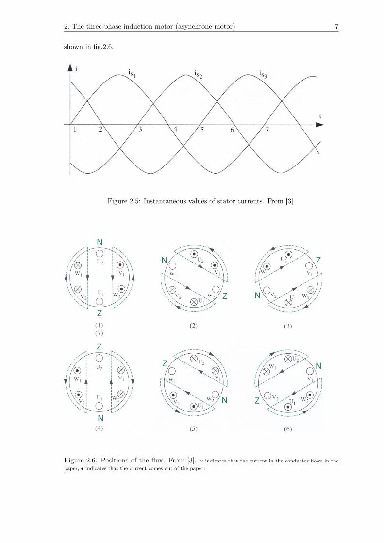
If a three-phase source (net) is connected to U1, V1 and W1, alternating currents (AC)will flow in the windings. The currents will have the same values but will be displaced intime by an angle of 120. They produce a magnetomotive force which creates a magneticflux. The latter flux will be studied in detail. The corporation of the three currents willcreate a flux pattern that rotates in time. A graphical representation is visualized in fig.2.5and fig.2.6. Fig.2.5 represents the three-phase currents in the stator windings, while themagnetical field that is created in the stator by the currents, the stator rotation field, is
2. The three-phase induction motor (asynchrone motor) 7
shown in fig.2.6.
Figure 2.5: Instantaneous values of stator currents. From [3].
Figure 2.6: Positions of the flux. From [3]. x indicates that the current in the conductor flows in thepaper, • indicates that the current comes out of the paper.

2. The three-phase induction motor (asynchrone motor) 8
Consider fig.2.3, a two-pole induction motor. In one period of the three-phase current, thestator rotation field makes one complete turn (two pole pitches) during one cycle (fig.2.6).Therefore, the rotational speed of the field depends, upon the duration of one cycle, whichin turn depends on the frequency of the source. If the frequency is 50 Hz, the resulting fieldmakes one turn in 1/50 s, equal to 3000 rounds per minute. If now a four-pole inductionmotor would be considered, the flux would only rotate halve a turn (two pole pitches)during one cycle, 1500 rounds per minute.What is explained here is noting else then the Law of Ferraris, equation (2.1).
Finally it is good to notice that the created flux is not sinusoidal. To approach the latter,the number of coils along the stator-side needs to fluctuate.
2.3.3 Starting characteristics of a Squirrel-Cage motor
Consider the situation where the stator of the induction motor is connected to the three-phase net, with the rotor locked. The stator will create a rotating field across the rotorand will induce a voltage over the rotor. This is an AC-voltage because each conductor iscut by a N-pole followed by a S-pole.Because the rotor is short-circuited by the end-rings, the induced voltage will cause a largecurrent flowing through the rotor. These current-carrying conductors are cut4 by a fluxcreated by the stator and all the conductors experience a strong mechanical force. Theseforces intent to drag the rotor along with the rotation field, the rotor is liable to a torque.
2.3.4 Acceleration of the rotor
Consider the situation from subsection 2.3.3. Releasing the rotor from its lock will makethe force able to rapidly accelerate the rotor along the direction of the rotation field, asit picks up speed. The relative speed difference between the field and the rotor decreases.This causes both the value and the frequency of the induced voltage to decrease becausethe rotor is cut more slowly. The speed will continue to increase but will never catch upto the synchrone speed of the field, otherwise there would be no inductionvoltage (Law ofMaxwell)5.
2.3.5 Motor under load
Consider the motor at a stable speed. If a load (an extra torque in opposite direction ofthe field) is applied to the shaft, the speed of the motor will start to decrease. The relativespeed difference will increase and a larger torque will be created. The motor will reach astable point when the extra created torque is exactly equal to the loaded torque.
4Cut: the current-carrying conductor flows trough the created flux, conductors ‘cut’ the flux in twopieces.
5Therefore the described motor is called asynchrone motor. For example a 2-pole asynchrone motorrotates with rotation frequency of 3000 rpm, but the rotor will only rotate with a speed of 2900 rpm. Therotor current-carrying conductors will cut the rotation field with a speed of 100 rpm.

2. The three-phase induction motor (asynchrone motor) 9
The speed that the motor will finally have, lies lower then the speed before the extra torquewas added.
2.3.6 Slip
The speed difference between the rotor (n) and the stator rotation field (nS) is called theslip (g):
g =nS − n
nS(2.2)
New parameter(s):g = the slip [%]
n = speed of the rotor [rpm]
n = nS(1− g) (2.3)
The slip is a fraction of nS and is mostly expressed in %. The slip scale is a linear scale,at stagnation (n = 0) g = 1 and at synchrone speed (n = nS) g = 0. The slip can also benegative n > nS , then it is called generator working. In that case the speed of the rotor isfaster then the stator field (e.g. when an external drive is used, for example a two-pole, ata four-pole 50Hz motor and let it turn at 1560 rpm). The asynchrone motor will work asan asynchrone generator and will put power back into the net.
Rotor frequency
The frequency of the rotor (fR) depends on the speed difference between the stator rota-tion field (nS) and the rotor (n), equation (2.1) for fR:
fR =p.(nS − n)
60(2.4)
with (2.2):fR =
p.g.nS
60= g.
p.nS
60(2.5)
and, (2.1):fS = p.nS60 , so:
fR = g.fS (2.6)
New parameter(s):fR = frequency of the rotor [Hz]
Rotor-emk
The rotor-emk is the voltage created by the rotation field across the rotor.With a stagnating rotor, the speed6 difference between the rotor conductor (vrotor, speed
6The speed of the rotor can be expressed in n [rpm], ω [rad/s] or in v [m/s]. v = ω.R, with R theradius of the circle where the observant point is moving, the link between n and ω is explained later on.

2. The three-phase induction motor (asynchrone motor) 10
of the rotor) and stator rotation field (vstator, speed of the rotation field) will be nS . Therotor-emk at stagnation (ERstag) is distracted from the equation (A.2):
ERstag = B.l.vstator (2.7)
The rotor-emk at a certain speed (ER) will only be determent by the speed differencebetween the rotation field and the rotor:
ER = B.l.(vstator − vrotor) (2.8)
With equation (2.3) in function of v, vrotor = vstator(1− g):
ER = B.l.g.vstator = g.(B.l.vstator) (2.9)
In other words:ER = g.(ERstag) (2.10)
New parameter(s):
vstator = speed of the rotation field [m/s]
vrotor = speed of the rotor (conductors) [m/s]
ER = voltage over the rotor windings at a slip g [V ]
ERstag = voltage over the rotor windings at stagnation [V ]
Speed rotor rotation field
The Law of Maxwell states that a changing magnetic field introduces an electrical field.But the opposite is also true, a changing electrical field introduces a magnetic field. Thismeans that the rotating electrical field of the rotor produces a rotating magnetic field (ΦR).The rotor currents, with frequency fR = g.fS , create a magnetomotive force (MMF), whichcreates a magnetic flux that rotates with a speed nR = g.nS in respect to the rotor.The rotor rotates at a speed n. Where n = (1− g).nS (2.3).The rotor rotation field will move with respect to the stator at a speed of:
n + nR = nS .(1− g) + g.nS = nS (2.11)
New parameter(s):
ΦR = rottor magnetic rotation field [Wb]
nR = relative speed of the rotor field in respect to the rotor [rpm]
Consequently the stator will always see the rotor at the synchrone speed. In other words,even if the slip changes, the stator will always see the rotor in the same way.

2. The three-phase induction motor (asynchrone motor) 11
2.4 T-equivalent scheme
In this section the T-equivalent scheme is described. It is the mathematical representationof the induction motor and is used for calculations in steady-state.The T in T-equivalent comes from the outlook of the scheme, a T can be recognized.
2.4.1 Leak inductances - equivalent transformator
Leak inductance is similar as with a transfo7. It consists of the rotation field-lines of thestator field, that do not reach the rotor coils, and the field-lines from the rotor coils, thatdo not reach the stator coils. The latter are called the stator and rotor leak inductances.Similar to a transfo, the following equivalent scheme can be applied [3]:
Figure 2.7: Equivalent transfo for one-phase inductionmotor
New parameter(s):
US1 = net phase voltage [V ]
ES1 = voltage in the stator coil [V ]
NS = number of windings of one stator coil [−]
NR = number of windings of one rotor coil [−]
I, iS = stator-phase current (I=absolute) [A]
I, iR = rotor-phase current(I=absolute) [A]
Ir = real rotor-phase current [A]
RS = stator winding resistance [Ω]
RR = rotor winding resistance [Ω]
Rr = real resistance of one phase [Ω]
L0 = magnetic inductance, this is the common (coupled) self inductance
between the stator and the rotor, and is responsible for the flux
ΦS1 in one-phase [H]
ΦS1 = flux in one fase [Wb]
Lr = real leak inductance of one phase [H]
XS = stator reactance [Ω]
ωS = speed of the stator magnetic rotation field [rad/s]
ωR = speed of the rotor [rad/s]
σS = stator scatter coefficient [−]
σR = rotor scatter coefficient [−]
7Not covered in this thesis. For more information on this subject [3],[4] and [5] can be recommended.
2. The three-phase induction motor (asynchrone motor) 12
Notice that, to express the speed, ωR [rad/s] is used instead of nR [rpm]:(In general)
ωR =2.π.nR
60(2.12)
2.4.2 T-equivalent induction motor
With the real rotor resistances of one-phase (Rr) and the real rotor leak inductances ofone-phase (Lr), the rotor current (Ir) can be written as ((from fig.2.7) and the basic lawof electricity: Current = V olt
Resistances):
~Ir =~ER
Rr + j.ωR.Lr(2.13)
To draw the T-equivalent scheme like fig.2.8, there has to be worked at the same frequencyon rotor-side (left-side) as on stator-side (right-side). This is true when the rotor-side is instagnation:Equation (2.13):
~Ir =~ER
Rr + j.ωR.Lr(2.14)
with (2.10), (2.14) becomes:
~Ir =g. ~ERstag.
Rr + j.ωR.Lr(2.15)
=~ERstag.
Rrg + j.ωR
g .Lr
(2.16)
Replacing ωRg by ωS :
~Ir =~ERstag.
Rrg + j.ωS .Lr
(2.17)
Furthermore the winding ratio from the stator coil to the rotor coil (idem transfo) has tobe taken into account:
RR =(
NSNR
)2(Rr) → RR
g = Rrg
(NSNR
)2
and:
σR.L0 =(
NSNR
)2(Lr) → XR = ωS .σR.L0
These equations lead to fig.2.8. Notice that the rotor is connected on ES1 = ERstag.(
NSNR
)and the rotor current is given by IR = Ir.
(NSNR
).
2. The three-phase induction motor (asynchrone motor) 13
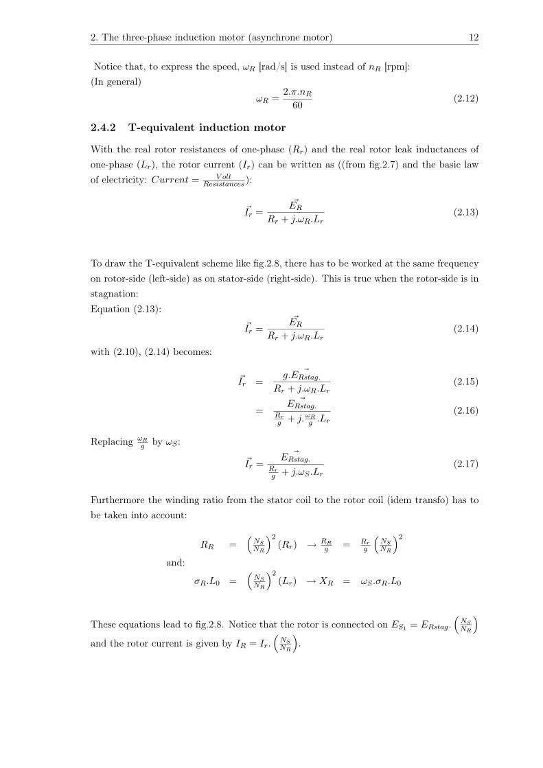
Figure 2.8: T-equivalent
New parameter(s):I, iµ = magnetazing current(I=absolute) [A]
LS = stator self induction =L0.(1 + σS) [H]
LR = rotor self induction =L0.(1 + σR) [H]
XR = rotor reactance [Ω]
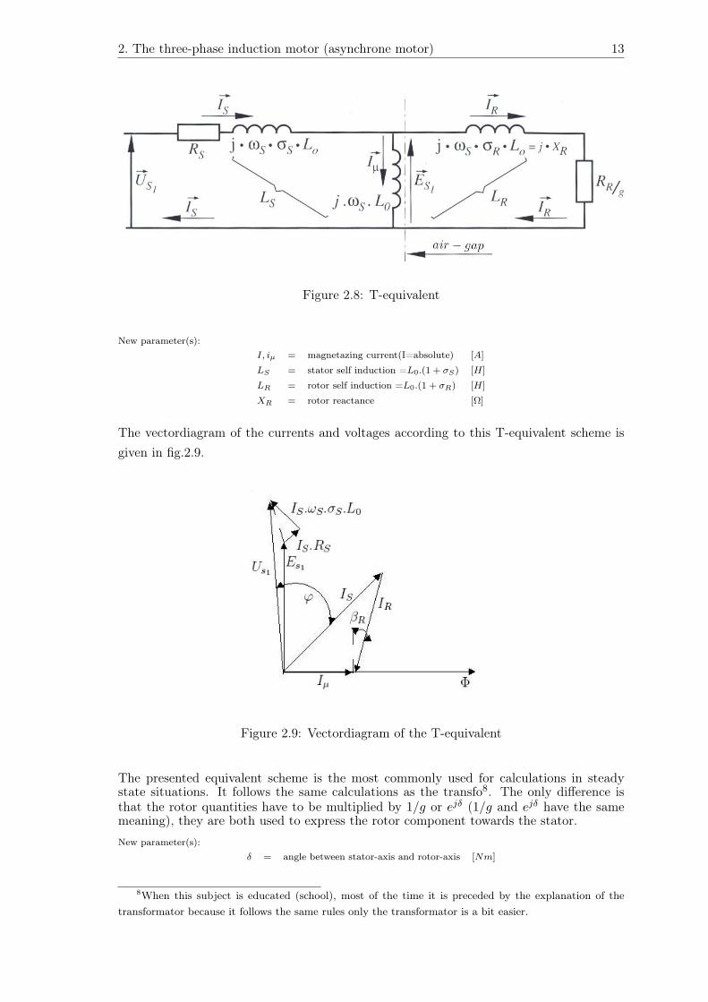
The vectordiagram of the currents and voltages according to this T-equivalent scheme isgiven in fig.2.9.
Figure 2.9: Vectordiagram of the T-equivalent
The presented equivalent scheme is the most commonly used for calculations in steadystate situations. It follows the same calculations as the transfo8. The only difference isthat the rotor quantities have to be multiplied by 1/g or ejδ (1/g and ejδ have the samemeaning), they are both used to express the rotor component towards the stator.
New parameter(s):δ = angle between stator-axis and rotor-axis [Nm]
8When this subject is educated (school), most of the time it is preceded by the explanation of thetransformator because it follows the same rules only the transformator is a bit easier.
2. The three-phase induction motor (asynchrone motor) 14
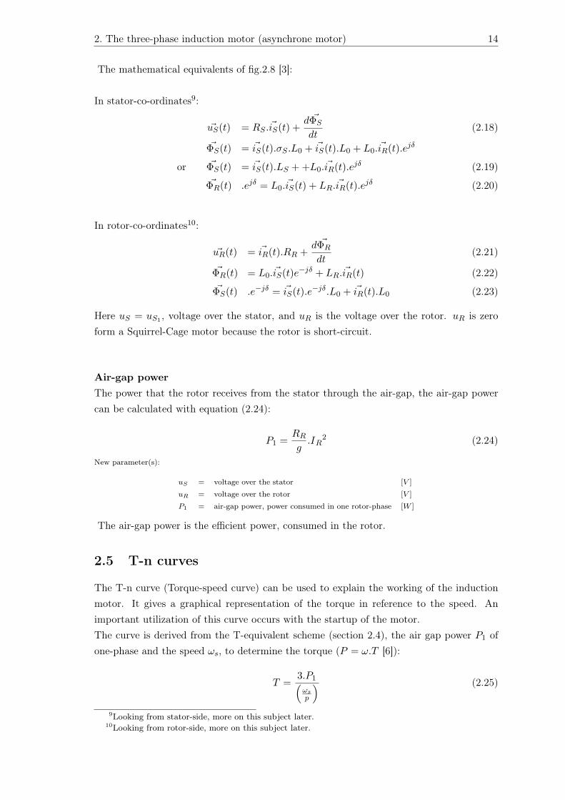
The mathematical equivalents of fig.2.8 [3]:
In stator-co-ordinates9:
~uS(t) = RS . ~iS(t) +d ~ΦS
dt(2.18)
~ΦS(t) = ~iS(t).σS .L0 + ~iS(t).L0 + L0. ~iR(t).ejδ
or ~ΦS(t) = ~iS(t).LS + +L0. ~iR(t).ejδ (2.19)~ΦR(t) .ejδ = L0. ~iS(t) + LR. ~iR(t).ejδ (2.20)
In rotor-co-ordinates10:
~uR(t) = ~iR(t).RR +d ~ΦR
dt(2.21)
~ΦR(t) = L0. ~iS(t)e−jδ + LR. ~iR(t) (2.22)~ΦS(t) .e−jδ = ~iS(t).e−jδ.L0 + ~iR(t).L0 (2.23)
Here uS = uS1 , voltage over the stator, and uR is the voltage over the rotor. uR is zeroform a Squirrel-Cage motor because the rotor is short-circuit.
Air-gap powerThe power that the rotor receives from the stator through the air-gap, the air-gap powercan be calculated with equation (2.24):
P1 =RR
g.IR
2 (2.24)
New parameter(s):
uS = voltage over the stator [V ]
uR = voltage over the rotor [V ]
P1 = air-gap power, power consumed in one rotor-phase [W ]
The air-gap power is the efficient power, consumed in the rotor.
2.5 T-n curves
The T-n curve (Torque-speed curve) can be used to explain the working of the inductionmotor. It gives a graphical representation of the torque in reference to the speed. Animportant utilization of this curve occurs with the startup of the motor.The curve is derived from the T-equivalent scheme (section 2.4), the air gap power P1 ofone-phase and the speed ωs, to determine the torque (P = ω.T [6]):
T =3.P1(
ωsp
) (2.25)
9Looking from stator-side, more on this subject later.10Looking from rotor-side, more on this subject later.

2. The three-phase induction motor (asynchrone motor) 15
with equation (2.24):
T =3.p
ωs.
(RR
g
).I2
R (2.26)
using (2.3):
T =3.p
ωS.
(RR.ωs
ωR
).I2
R (2.27)
and (2.17):
T =3.p.RR
ωR.
E2S1(
RR.ωSωR
)2+ (ωS .σR.L0)
2(2.28)
With the assumption that US1 ≈ ES1(= ΦS1 .ωS), the equation for the moment of thetorque:
T =3.p.RR
ωR.
Φ2S1[(
RRωR
)2+ (σR.L0)
2
] (2.29)
The maximum of this curve is found by dTdωR
= 0
ωR =RR
σR.L0(2.30)
Replacing ωR in (2.29) by (2.30) gives:
Tmax =3.p.ΦS1
2
2.σR.L0(2.31)
This derivation leads to the following curve (fig.2.10):
Figure 2.10: AC-torque-speed-curve

2. The three-phase induction motor (asynchrone motor) 16
On fig.2.10 a slip scale is added.
Remarks
KiptorqueThe maximum torque is called the kiptorque: Tk = Tmax
1. The maximum torque will occur at a pulsation of the rotor current, given by: equation(2.30) The maximum torque is actually situated on a time shift (ω = 2.π
T = 2.π.f)∆ω = ωR = RR
σR.L0of the synchrone speed. So the kiptorque occurs at:
ω = ωS −RR
σR.L0(2.32)
Formula (2.32) shows that moment where the maximum torque occurs can be influ-enced by the rotor resistance RR.
2. From equation 2.31 it can be seen that the maximum of kiptorque is independent ofRR
Generator workingFor negative values of ωR (ω > ωS) the torque (2.29) will take negative values. In otherwords the T-n curve will be symmetric in respect to the point ωR=0, at the synchronespeed.
- For 0 < ω < ωS the machine works as a motor
- For ω > ωS the machine works as a generator (negative torque at a positive rotationspeed)
New parameter(s):T = moment of torque, the torque [Nm]
Tmax = maximum torque [Nm]
Tk = kiptorque [Nm]

Chapter 3
Vector control of an induction motor
3.1 Introduction
3.1.1 Electronically controlled induction motor
The induction motor is the most commonly used motor, it has many advantages over othertypes of motors, but also some disadvantages. The greatest disadvantage is the issue ofcontrol. A lot of time and money is investigated in the research and development of controlstrategies for the induction motor. They are trying to control two important physicalvariables on the shaft of the motor, the speed and the torque. Applying an electricalcircuit makes the controle of these variables possible. Two different types of control canbe distinguished:
• Directing of the motorspeed (scalar drive)
• Regulating the of speed and (or) torque of an induction motor ((flux)-vector regula-tion)
In the first control strategy an electronic convertor is added in between the net and themotor, where only the height of the motorflux and the torque is controlled.In the second control strategy not only the amplitude of the flux, but also the phase iscontrolled. E.g. field oriented control of an induction motor to become a good dynamicbehaviour.Both methods have there advantages and downsizes.Only a summary is given:
17

3. Vector control of an induction motor 18
1. Scalar drive
• Advances
– Cheap convertor
– No feedback needed
• Downsizes
– Workingpoint of motor is notknown
– Torque is not controlled
2. (Flux)-Vector Control
• Advances
– Accurate speed regulation
– Good torque regulation
– Full torque until stagnation
– Approaches the dynamicalcharacteristics of DC-drive
• Downsizes
– Feedback needed
– Expensive convertor
A vector controlled drive is dynamically better then a scalar controlled drive. It is fast andmore precise.Because the price of electronics has decreased in previous decennia and it will probablykeep decreasing, (Flux)-vector control will take/has taken the overhand over the scalardrive due to the more accurate and faster control.
3.1.2 Dynamic model of AC-motor
Although the traditional T-equivalent circuit (section 2.8) has been widely used in steady-analysis and design of AC-motors, it is not appropriate to predict the dynamic behaviourof the motor. In order to understand and analyze vector control of an AC-motor drive, adynamic model is necessary. As the application of AC-motors has continued to increaseover this century, new techniques have been developed to aid in their analysis. The sig-nificant breakthrough in the analysis of three-phase AC-motors was the development ofthe reference frame theory. Using these techniques, it is possible to transform the motormodel to another reference frame1 and simplify the complexity of the mathematical motormodel.
In the following section, the dynamic model equations will be developed on a rotatingreference frame which makes the description characteristics of the induction motor moreeasily2.It will be shown that choosing a reference frame in which the rotor flux lies on the d-axis,the dynamic equations of the induction motor are simplified and likewise to a DC-motor.Further, the mathematical base of field oriented control will be calculated.
Trying to make a clear structured explanation, this chapter will start by introducing thetwo-phase induction motor and the link between two-phase and three-phase motor will bemade. So the explanation of the reference frame flows in a clear pattern.
1For steady-state analyze, the iS1 , iS2 and iS3 reference frame is used. More will be explained in thischapter.
2These are developed for induction motors but are equally applicable to synchronous motors.

3. Vector control of an induction motor 19
3.2 Two-phase induction motor in sinus-regime
Two-phase nets were almost exclusively used in the begin years of electrical distributionand are in principle nets with four conductors (three if the neutral is common). Theyconsisted of two AC-voltages,uα and uβ , that are positioned 90 in respect to each other(fig.3.1). A two-phase Squirrel-Cage motor can be build, in analogy with a three-pase
(a) uα and uβ shifted in time (b) Representation of the four conductors
Figure 3.1: Characteristics of a two-phase net
induction motor, out of coils (α and β) that are moved 90 in space. This is schematicallyrepresented in fig.3.2.Connecting the coils to the proposed net (uα, uβ) will create two currents (iα, iβ) that aremoved 90 in time.
Figure 3.2: Two-phase motor, basic structure
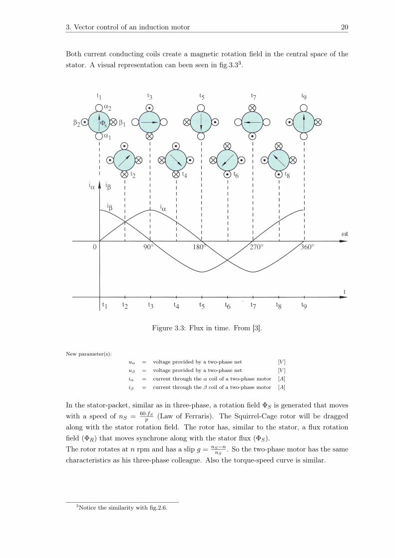
3. Vector control of an induction motor 20
Both current conducting coils create a magnetic rotation field in the central space of thestator. A visual representation can been seen in fig.3.33.
Figure 3.3: Flux in time. From [3].
New parameter(s):uα = voltage provided by a two-phase net [V ]
uβ = voltage provided by a two-phase net [V ]
iα = current through the α coil of a two-phase motor [A]
iβ = current through the β coil of a two-phase motor [A]
In the stator-packet, similar as in three-phase, a rotation field ΦS is generated that moveswith a speed of nS = 60.fS
p (Law of Ferraris). The Squirrel-Cage rotor will be draggedalong with the stator rotation field. The rotor has, similar to the stator, a flux rotationfield (ΦR) that moves synchrone along with the stator flux (ΦS).The rotor rotates at n rpm and has a slip g = nS−n
nS. So the two-phase motor has the same
characteristics as his three-phase colleague. Also the torque-speed curve is similar.
3Notice the similarity with fig.2.6.

3. Vector control of an induction motor 21
3.3 Three-phase to two-phase transformation
Consider again a three-phase induction machine where the stator coils are provided bythree voltages uS1 , uS2 and uS3 . The vectorial addition of these three voltages in space,~uS = ~uS1 + ~uS2 + ~uS3 , is called the stator voltage vector.
New parameter(s):~uS = stator voltage vector [V ]
~iS = stator current vector [A]
In fig.3.4, the stator voltage vector is drawn on two different moments in time (two mo-ments, t1 < t2, uS1 is positive and uS2 and uS3 are negative (the voltages are dephased120 in respect to each other)). If ~us would be followed over a whole period, it would rotate360.
Figure 3.4: Three-phase voltage moving in time
A similar construction with the three-phase currents iS1 , iS2 and iS3 can be made. Insteadof the voltage, the stator current vector can be determined ~iS = ~iS1 +~iS2 +~iS3 . Thecomponents of ~iS can be determined in a new defined two-axis system (α and β) (fig.3.5),the α-β reference frame.
Figure 3.5: Stator current vector in a new reference frame

3. Vector control of an induction motor 22
Analyzing the current iα according to the α-axis, equation (3.1) can be derived:
iα = iS1 − iS2 × sin 30− iS3 × sin 30 = iS1 −iS2 + iS3
2(3.1)
And with:is1 + is2 + is3 = 0 (Kirchoff) (3.2)
(3.1) becomes:
iα =32iS1 (3.3)
The current iβ , along the β-axis is given by equation (3.4):
iβ = 0 +√
32× iS2 −
√3
2× iS3 =
√3
2× (iS2 − iS3) (3.4)
What becomes with (3.2):
iβ =√
32
iS1 +√
3iS2 (3.5)
The equations (3.3) and (3.5) are seen as the three-phase to two-phase transformation inthe case of a symmetric three-phase system, also called the Clark-transformation. Withanalogy to the currents, the expressions for the components of the voltages can be writtenas:
uα =32× uS1 , uβ =
√3
2× (uS2 − uS3) (3.6)
From equation (3.6) is concluded that the absolute value of ~us is equal to 3/2 time uS1 ,the amplitude of one phase voltage. This is visualized in fig.3.4. Because the voltage is 3/2the voltage of one phase, the flux ΦS , that is linearly with the voltage, will be 3/2 timesthe flux of one phase.
ΦS =32ΦS1 (3.7)
The inverse out of formula (3.3) and (3.4) can also be qualified:
iS1 =23× iα, iS2 =
1√3× iβ −
13× iα, iS3 = − 1√
3× iβ −
13× iα (3.8)
This is called the inverse Clark-transformation.
3. Vector control of an induction motor 23
However, the Clark transformation, equally applied on both phase currents and voltages,is not power invariant:
P (t) = uS1 .iS1 + uS2 .iS2 + uS3 .iS3 6= uα.iα + uβ .iβ (3.9)
uα.iα + uβ .iβ =32uS1
32iS1 +
(√3
2uS1 +
√3uS2
).
(√3
2iS1 +
√3iS2
)= 3uS1iS1 + 3uS2iS2 +
32uS2iS1 +
32uS1iS2
=32[uS1iS1 + uS2iS2 + (−uS1 − uS2)(−iS1 − iS2)]
=32[uS1iS1 + uS2iS2 + uS3iS3 ] =
32P (t) (3.10)
So if power (P) is calculated, a scaling factor 23 has to be considered to guarantee the power
invariance.In other studies, different derivations are used to make the power invariant. Most timesa factor is added to the currents and voltages. In appendix B one possibility is explained[7]. The study where appendix B is derived from considers a zero component (involvingharmonics) next to iα and iβ . However, the zero-component is required neither for motorcontrol nor for describing the dynamic motor behaviour. Therefore the zero-component isneglected in next chapters. It should be noticed that later when talking about multi-phasemotors, the zero-component reconsidered and more explained.
Conclusion
Sending through coil α of the two-phase motor a current iα = 32 .iS1 and through β a
current iβ =√
32 (iS2 − iS3) will make the two-phase motor equivalent (same flux, torque
and slip) to the three-phase motor (with stator currents iS1 , iS2 and iS3) out of chapter 2.In this way, the following study of the equivalent two-phase induction is directly applicableon three-phase motors4.
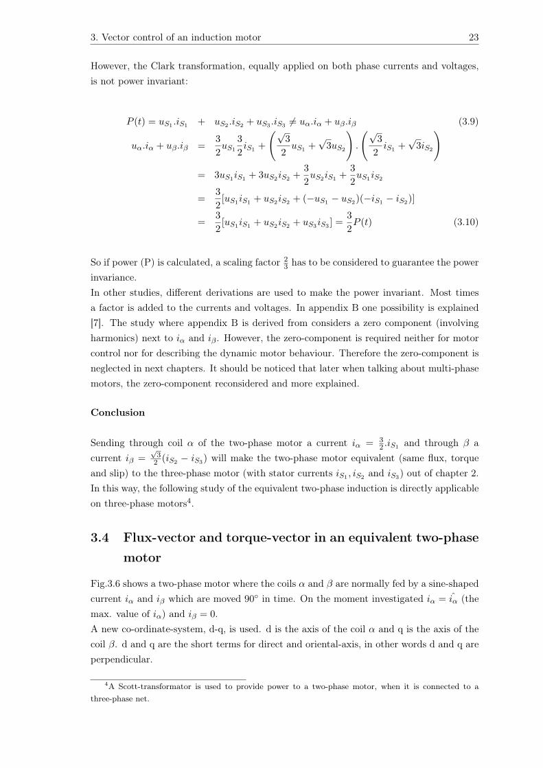
3.4 Flux-vector and torque-vector in an equivalent two-phasemotor
Fig.3.6 shows a two-phase motor where the coils α and β are normally fed by a sine-shapedcurrent iα and iβ which are moved 90 in time. On the moment investigated iα = iα (themax. value of iα) and iβ = 0.A new co-ordinate-system, d-q, is used. d is the axis of the coil α and q is the axis of thecoil β. d and q are the short terms for direct and oriental-axis, in other words d and q areperpendicular.
4A Scott-transformator is used to provide power to a two-phase motor, when it is connected to athree-phase net.
3. Vector control of an induction motor 24
Figure 3.6: Two-phase motor, representedby two coils.
Figure 3.7: Flux forming by the D coil in atwo-phase motor
3.4.1 Flux component
Replacing coils α and β by two fictive coils D and Q (fig.3.7) and sending a DC-currentid, that has the same size as iα, through D will create a flux ΦR. The component id iscalled the flux forming component or the flux vector. Adjusting the DC-current id fromzero until regime value, will make the flux change from zero to regime value ΦR.During the change of the flux, an inducted emk is induced in the rotor-conductors and,with closed rotor chain, currents will flow as indicated in fig.3.7.Because of the selfinductance of the rotor, it will take up to five times the rotor timecon-stant τR = LR/RR for the flux to reach its regime value. On that moment, ΦR is constantand the inductioncurrent in the rotor disappears (Law of Maxwell). τR, the rotor timecon-stant, is normally more than hundred ms. In the T-equivalent of an asynchrone motor, L0
is called the magnetic induction. So the flux ΦR can be written as ΦR = L0.id. This is notexact because the rotor time-constant takes for a (exponential) delay. The exact value is:
τR.dΦR
dt+ dΦR = L0.id (3.11)
New parameter(s):id = direct current, flux forming component [A]
τR = rotor timeconstant [s]
Developing this further gives:
ΦR = L0.id[1− e−t/τr ] (3.12)
In other words the flux will increase until its regime value (ΦR = L0.id) is reached.
3.4.2 Torque component
Assuming the situation in fig.3.8 where a flux, ΦR, has reached its regime value. A DC-current, iq, is sent through coil Q. Consequently a flux ΦQ emerges in coil Q. This flux

3. Vector control of an induction motor 25
Figure 3.8: Two-phase motor torqueforming Figure 3.9: DC-machine
will, in the time it raises from zero to regime, take care of inductionvoltage and -currentin the rotor (Law of Maxwell). Now, because this current-carrying conductor lies in amagnetic rotation field, it experiences a mechanical force (the Lorentz force). This resultsin a torque that makes the rotor to rotate.
Summarizing, it can be said that id is responsible of creating a flux ΦR (flux forming com-ponent) and iq is responsible for the torque (torque forming component).
What has been explained above is virtually the same as what happens in a DC-motor,namely the currentconduction (ankercurrent) works on the flux (ΦR) to create a torque.
New parameter(s):iq = quadrature current, torque forming component [A]
ΦQ = flux by coil Q [Wb]
DC-motor
Investigating the DC-motor (fig.3.9), it is found that the torque is very easily controllable[6]:
T ≈ ~Φ.~I to be exact Tem = k2. ~Ia.~Φ (3.13)
New parameter(s):
Tem = electromechanical torque [Nm]
k2 = a machineconstant [−]
Φ = the flux inside the DC-motor [Wb]
Ia = the constant current through the windings of the DC-motor [A]
Taking the flux constant, the torque will only depend on the current. In this way the
3. Vector control of an induction motor 26
torque is controllable just by adjusting one parameter, the current. This is the reasonwhy controle of DC-motors is very easy. Another surplus is that flux and current areperpendicular, the vector-product of ~Ia and ~Φ is maximized (sin 90 = 1). Vector controlis based on the same reasoning as the DC-control: keeping the flux constant, keeping theflux and current perpendicular and in this way creating an environment that is very easilycontrolled, only by controlling two parameters.
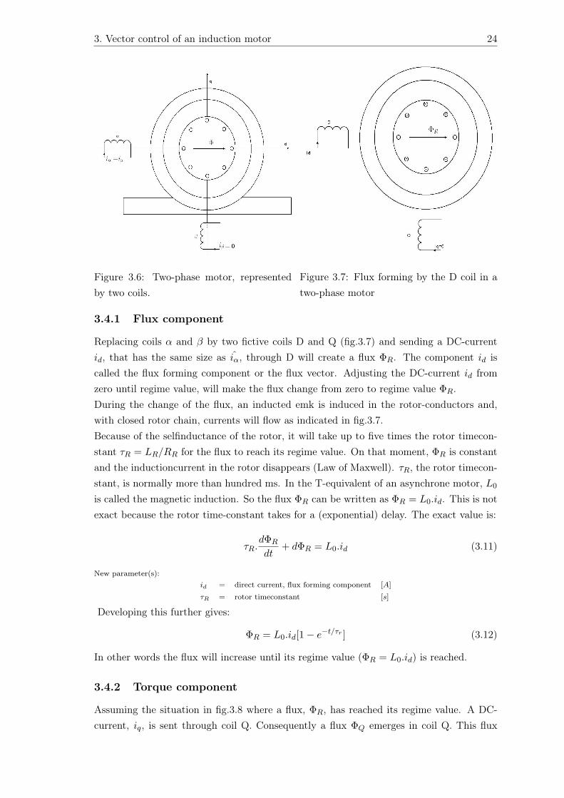
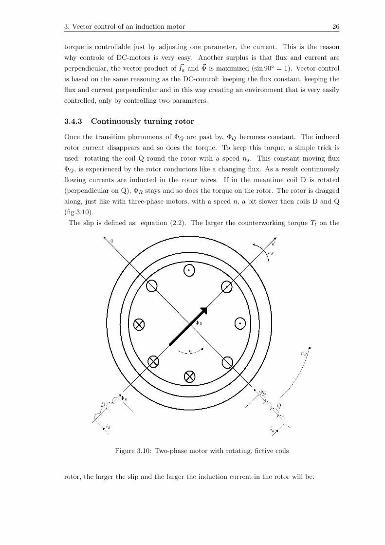
3.4.3 Continuously turning rotor
Once the transition phenomena of ΦQ are past by, ΦQ becomes constant. The inducedrotor current disappears and so does the torque. To keep this torque, a simple trick isused: rotating the coil Q round the rotor with a speed ns. This constant moving fluxΦQ, is experienced by the rotor conductors like a changing flux. As a result continuouslyflowing currents are inducted in the rotor wires. If in the meantime coil D is rotated(perpendicular on Q), ΦR stays and so does the torque on the rotor. The rotor is draggedalong, just like with three-phase motors, with a speed n, a bit slower then coils D and Q(fig.3.10).The slip is defined as: equation (2.2). The larger the counterworking torque Tt on the
Figure 3.10: Two-phase motor with rotating, fictive coils
rotor, the larger the slip and the larger the induction current in the rotor will be.

3. Vector control of an induction motor 27
FormulasDerived from fig.3.8, the torque changes linearly with the product of the flux ΦR and thecurrent in the rotor conductors. This current is however proportional to the flux Φq andso with the current iq:
Tem = k3.iq.ΦR (3.14)
With:
k3 = a machineconstant [−]
Expression (3.14) is identical with the one on the DC-motor: Tem = k2.Ia.Φ. By managingthe current iq in the equivalent two-phase motor, the torque is easily controllable, similarwith the DC-motor.
3.5 Co-ordination transformation
3.5.1 Transformation formulas
The flux- and torqueforming components of the fictive coils D and Q exist in reality out oftwo changing currents, iα and iβ , in the coils of the two-phase motor. These coils are fixedto the stator. The α and β axis are fixed to the stator in the way that the α-coil gives aflux along the α-axis and the β-coil along the β-axis.Knowing that the rotation field in the stator moves at a speed of ωs (fig.3.3), the rotoris dragged at a speed ω < ωs. The rotor creates a rotor flux ΦR which rotates at aspeed ωs similar to a three-phase motor. If the fictive coils, D and Q (and so the d-qco-ordinate-system), are rotating with the rotor flux ΦR, a new co-ordinate-system can beused (fig.3.11) also called rotating reference frame.The current iα decomposed:
• d-way: idα = iα.cosλ
• q-way: iqα = −iα.sinλ
The current iβ decomposed:
• d-way: idβ = iβ.sinλ
• q-way: iqβ = iβ.cosλ
The currents iα and iβ out of the stator-co-ordination-system (α, β) take care for thecurrent id and iq in a co-ordinate-system that rotates together with the rotor flux ΦR:
id = idα + idβ = iα. cos λ + iβ. sinλ (3.15)
iq = iqα + iqβ = iβ . cos λ− iα. sinλ (3.16)
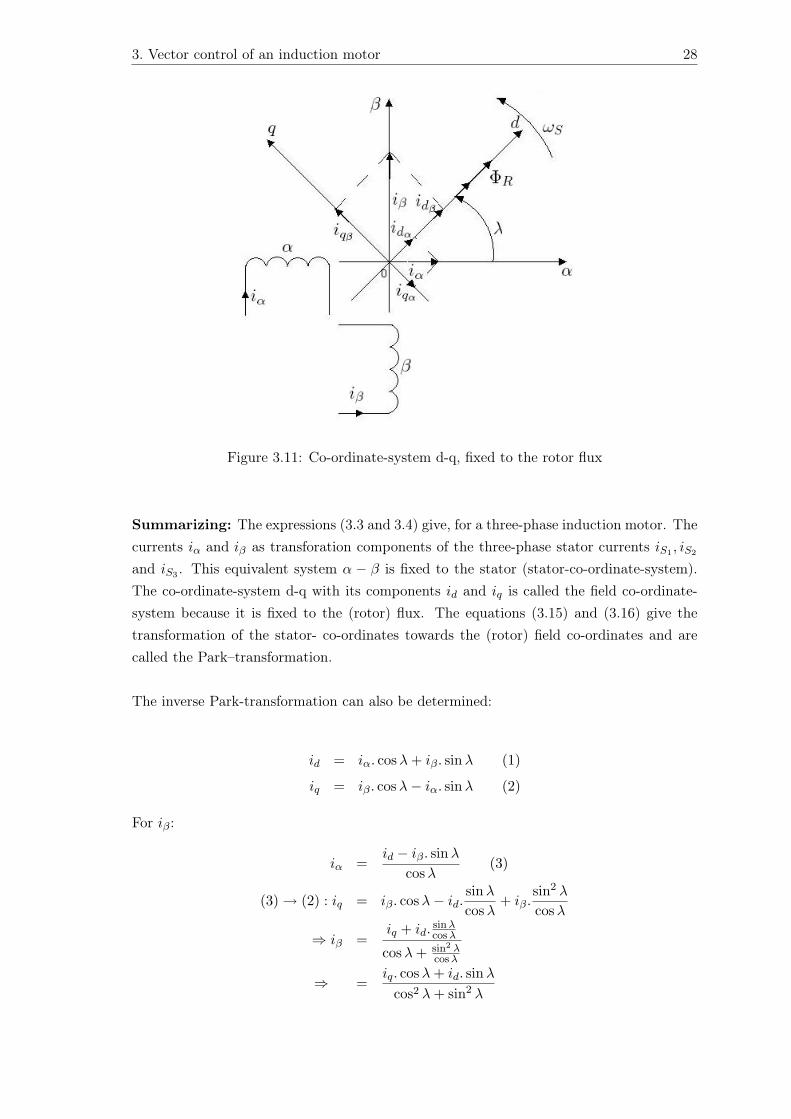
3. Vector control of an induction motor 28
Figure 3.11: Co-ordinate-system d-q, fixed to the rotor flux
Summarizing: The expressions (3.3 and 3.4) give, for a three-phase induction motor. Thecurrents iα and iβ as transforation components of the three-phase stator currents iS1 , iS2
and iS3 . This equivalent system α − β is fixed to the stator (stator-co-ordinate-system).The co-ordinate-system d-q with its components id and iq is called the field co-ordinate-system because it is fixed to the (rotor) flux. The equations (3.15) and (3.16) give thetransformation of the stator- co-ordinates towards the (rotor) field co-ordinates and arecalled the Park–transformation.
The inverse Park-transformation can also be determined:
id = iα. cos λ + iβ. sinλ (1)
iq = iβ. cos λ− iα. sinλ (2)
For iβ :
iα =id − iβ. sinλ
cos λ(3)
(3) → (2) : iq = iβ . cos λ− id.sinλ
cos λ+ iβ.
sin2 λ
cos λ
⇒ iβ =iq + id.
sin λcos λ
cos λ + sin2 λcos λ
⇒ =iq. cos λ + id. sinλ
cos2 λ + sin2 λ
3. Vector control of an induction motor 29
For iα:
iβ =iq + iα. sinλ
cos λ(4)
(4) → (1) : id = iα. cos λ + iq.sinλ
cos λ+ iα.
sin2 λ
cos λ
⇒ iα =id − iq.
sin λcos λ
cos λ + sin2 λcos λ
⇒ =id. cos λ− iq. sin λ
cos2 λ + sin2 λ
Knowing that cos2 λ + sin2 λ = 1 the inverse Park-transformation is given by:
iα = id. cos λ− iq. sin λ (3.17)
iβ = iq. cos λ + id. sin λ (3.18)
3.5.2 Notations in other co-ordinate-systems
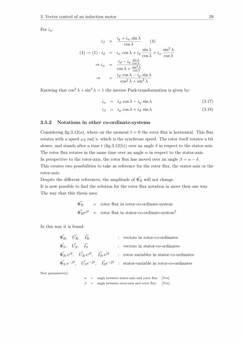
Considering fig.3.12(a), where on the moment t = 0 the rotor flux is horizontal. This fluxrotates with a speed ωS rad/s, which is the synchrone speed. The rotor itself rotates a bitslower, and stands after a time t (fig.3.12(b)) over an angle δ in respect to the stator-axis.The rotor flux rotates in the same time over an angle α in respect to the stator-axis.In perspective to the rotor-axis, the rotor flux has moved over an angle β = α− δ.This creates two possibilities to take as reference for the rotor flux, the stator-axis or therotor-axis.Despite the different references, the amplitude of ~ΦR will not change.It is now possible to find the solution for the rotor flux notation in more then one way.The way that this thesis uses:
~ΦR = rotor flux in rotor-co-ordinate-system
~ΦRejδ = rotor flux in stator-co-ordinate-system5
In this way it is found:
~ΦR, ~UR, ~IR : vectors in rotor-co-ordinates
~ΦS , ~US , ~IS : vectors in stator-co-ordinates
~ΦR.ejδ, ~UR.ejδ, ~IR.ejδ : rotor-variables in stator-co-ordinates
~ΦS .e−jδ, ~USe−jδ, ~ISe−jδ : stator-variable in rotor-co-ordinates
New parameter(s):α = angle between stator-axis and rotor flux [Nm]
β = angle between rotor-axis and rotor flux [Nm]
3. Vector control of an induction motor 30
Figure 3.12: Rotor flux, in (a) rotor- and (b) stator-co-ordinate system
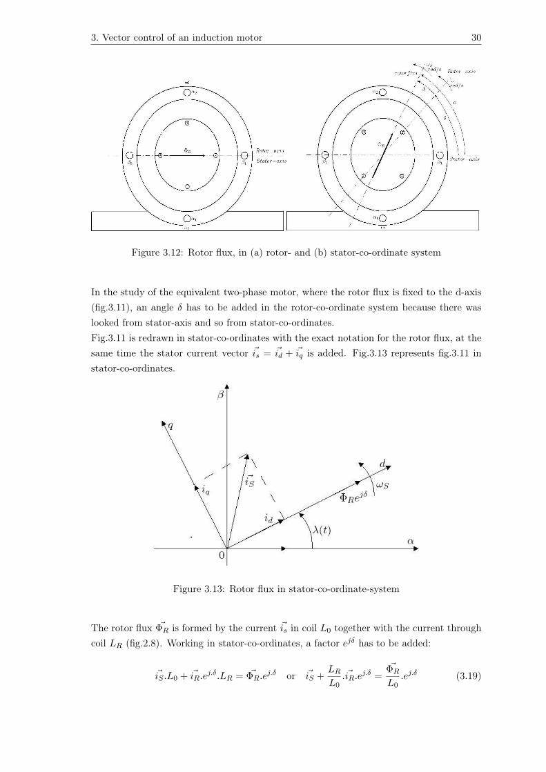
In the study of the equivalent two-phase motor, where the rotor flux is fixed to the d-axis(fig.3.11), an angle δ has to be added in the rotor-co-ordinate system because there waslooked from stator-axis and so from stator-co-ordinates.Fig.3.11 is redrawn in stator-co-ordinates with the exact notation for the rotor flux, at thesame time the stator current vector ~is = ~id + ~iq is added. Fig.3.13 represents fig.3.11 instator-co-ordinates.
Figure 3.13: Rotor flux in stator-co-ordinate-system
The rotor flux ~ΦR is formed by the current ~is in coil L0 together with the current throughcoil LR (fig.2.8). Working in stator-co-ordinates, a factor ejδ has to be added:
~iS .L0 + ~iR.ej.δ.LR = ~ΦR.ej.δ or ~iS +LR
L0. ~iR.ej.δ =
~ΦR
L0.ej.δ (3.19)
3. Vector control of an induction motor 31
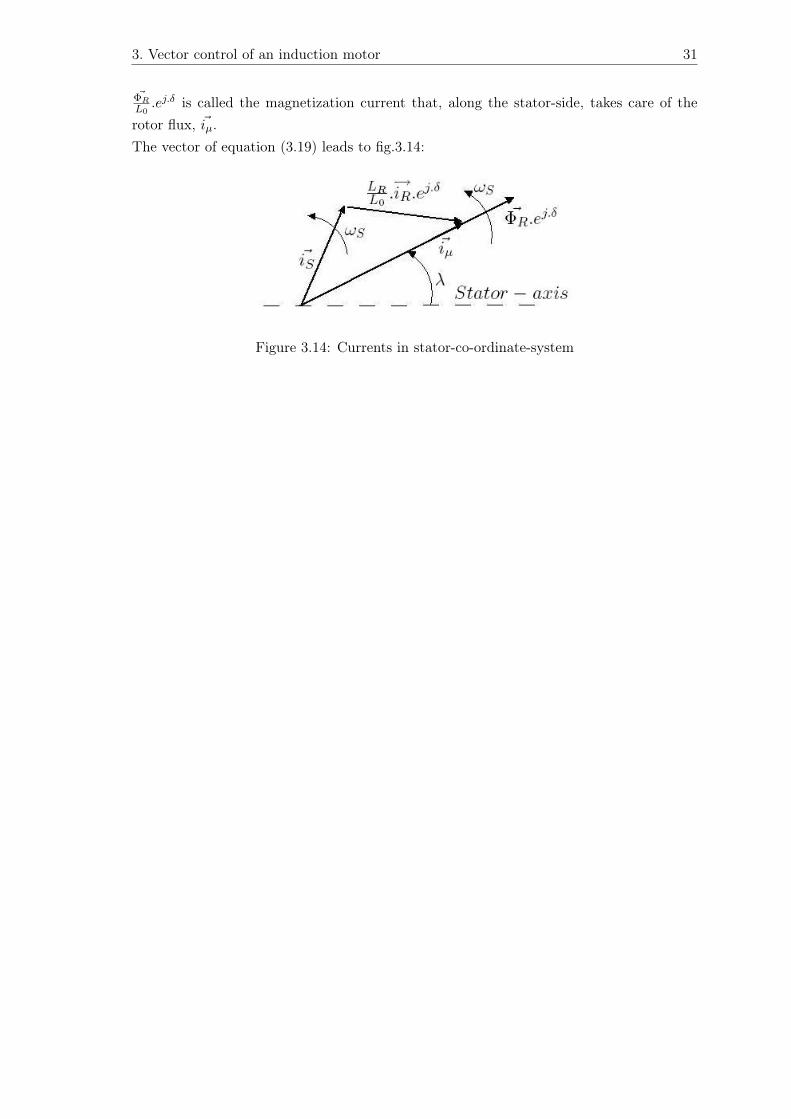
~ΦRL0
.ej.δ is called the magnetization current that, along the stator-side, takes care of therotor flux, ~iµ.The vector of equation (3.19) leads to fig.3.14:
Figure 3.14: Currents in stator-co-ordinate-system

Chapter 4
Mathematical formulas
4.1 Introduction
Adjustable speed drives1 with torque control are required in many applications, e.g. manu-facturing and transportation. Using AC-motors and high performance AC-drives that arecapable of controlling torque and flux independently offers several advantages over DC-motors and drives such as lower maintenance, smaller size and higher speeds. Comparedto DC-drives, the higher cost of AC-drives is in part compensated by a lower motor cost.Compared to uncontrolled AC-motors, the efficiency of inverter controlled AC-drives canbe vastly increased by flux optimization. This results in energy saving, which may becrucial in larger application.This chapter provides the fundamental mathematical formulas of a high-performance mo-tion control, employing the field oriented control technique also termed the ‘rotor fluxoriented type of vector control’.The goal of field oriented control is to maintain the amplitude of the rotor flux linkage ΦR
at a fixed value (except for field weakening operation or flux optimization) and only modifya torque-producing current component in order to controle the torque of the AC-motor.The mathematical formulas will be used to implement a model in matlab/simulink. Thelast section of this chapter will discuss field weakening and field oriented control, which isneeded for a more realistic model.
1A drive is a controller of the speed of a motor.
32

4. Mathematical formulas 33
4.2 Derivation
Combination of the vector diagram of fig.3.13 and fig.3.14 leads to fig.4.1. Fig.4.1 isa visualization of the currents and the flux through the motor. Using this figure, themathematical equivalent scheme in rotor-reference frame will be derived.
Figure 4.1: Field orientation
New parameter(s):
λ(t) = angle where the rotor flux on the moment t is rotated with
respect to the stator reference-axis []
θ(t) = angle between the stator current and the stator-axis []
~iµ = fictive magnetization current which is responsible
for the rotor flux: ΦR = L0.iµ [A]
~ΦR.ej.δ = rotor flux in stator-co-ordinates [Wb]
Because ~iS(t) and ~ΦR.ej.δ rotate at the same speed (ωS), the angle ε is independent oftime. This means that the stator current ~iS(t) has a fixed orientation with respect to therotor flux2. The currents id and iq are the field-co-ordinates of the the stator current inthe co-ordinate-system that rotates with the rotor flux. The field-co-ordinates id and iq
determine the stator current ~iS fig.4.1:
~iS(t) = id + j.iq (4.1)
4.2.1 Electromechanical torque
The electromechanical torque3 of the inductionmotor is proportional with the vectorialproduct of the stator and rotor current vector [3].Both vectors should naturally be defined in the same co-ordinate-system (iR.ejδ).Fig.4.2 shows the vectors in the stator co-ordinate-system.
2This is what Dr. Ir. Blaschke called field orientation, Dr. Ir. Blaschke can be seen as the ‘father’ ofvector control, he was the first to speak vector control.
3This is a small intermezzo, it is a topic that could have been placed anywhere in this work. But it isplaced here because it is needed in the next section.

4. Mathematical formulas 34
Figure 4.2: Electromechanical torque induction motor
The vectorial product of ~iS with ~iR.ejδ is the area of the parallelogram in fig.4.2 en is givenby:
iS .iR.ejδ. sin(π − λ) = iS .iR.ejδ. sin(λ). (4.2)
The torque is proportional to area of this parallelogram:
Tem = k1.iS .iR.ejδ. sin(λ) (4.3)
Neglecting the friction torque4, this last expression shows the torque (T) on the shaft ofthe motor, so that:
T ≈ Tem = k1.iS .iR.ejδ. sinλ (4.4)New parameter(s):
k1 = a machine constant
For the further study a triangle will be considered, formed by ~iS , ~iR.ejδ and ~iµ (fig.4.1).The torque is linearly proportional with the area of the triangle (times two).
4.2.2 Fictive magnetization current
In a Squirrel-Cage motor, the currents and voltages are easily measured along stator-side.On the other hand, the formulas used in the study of field orientation are relatively simpleif there would be considered an interaction between stator current vector and rotor flux.Moreover by choosing the rotor flux as reference, a complete decoupling between flux andcurrent appears.In the rotor-co-ordinate-system the rotor flux was found:
~ΦR(t) = L0. ~iS(t)e−jδ + LR. ~iR(t) (4.5)4More about the friction torque can be found in [4].

4. Mathematical formulas 35
The rotor flux in stator-co-ordinates becomes :
~ΦR.ejδ = L0. ~iS + LR. ~iR.ejδ (4.6)
In 3.5.1, fig.3.14 was divided. Here(
~iµ =~ΦR.ejδ
L0
)a fictive magnetizing current, along
stator-side, is responsible for the rotor flux:Out of fig.3.14 follows:
~iµ = ~iS +LR
L0. ~iR.ejδ (4.7)
So that:~iR =
L0
LR(~iµ − ~iS).e−jδ
The rotor flux in stator-co-ordinates:
~ΦR.ejδ = L0.~iµ (4.8)
and in rotor-co-ordinates:~ΦR = L0.~iµ.e−jδ (4.9)
Replacing ~iR and ~ΦR in equation ~uR(t) = ~iR(t).RR + d ~ΦRdt (2.21) and knowing that ~uR = 0
(Squirrel-Cage):
0 = RR.L0
LR(~iµ − ~iS).e−jδ +
d
dt.(L0.~iµ.e−jδ) (4.10)
Decomposing the derivative:
0 = RR.L0
LR(~iµ − ~iS).e−jδ + L0.
d~iµdt
.e−jδ − L0.j.dδ
dt.e−jδ.~iµ (4.11)
Divide by L0LR
gives:
0 = RR(~iµ − ~iS) + LR.d~iµdt
− j.LR.dδ
dt.~iµ (4.12)
With dδdt = ω and LR
RR= τR, this gives:
τR.d~iµdt + (1− jω.τR).~iµ = ~iS (4.13)
4.2.3 Moment of torque
As stated in subsection 4.2.1, the torque is linearly proportional with the triangle formedby ~iS , LR
L0. ~iR.ejδ and ~iµ.
This area can also be determined as5:
12.~iq.~iµ (4.14)
5A different way of working considers the component ~iS that is perpendicular on this rotor flux.

4. Mathematical formulas 36
so that:Tem = k2.iµ.iq (4.15)
With: ΦR = L0.iµ equation (4.15) becomes:
Tem = k3.iq.ΦR (4.16)
New parameter(s):
k3 = a machine constant: k3 = 3p2
. L0LR
p is the number of pole pares
4.2.4 Mathematical model in field-co-ordinates
With ~iµ = iµ.ejλ, (4.13) becomes6:
~iS = τR.d
dt(iµ.ejλ) + (1− jω.τR).iµ.ejλ (4.17)
Decomposing the derivative:
~iS = τR.ejλ.diµdt
+ τR.iµ.j.dλ
dt.ejλ + (1− jω.τR).iµ.ejλ (4.18)
Dividing by ejλ and dλdt = ωS .
~iS .e−jλ = τR.diµdt
+ τR.iµ.j.ωS + (1− jω.τR).iµ (4.19)
Out ~iS(t) = iS .ejθ follows:
~iS .e−jλ = iS .ej(θ−λ) = iS .ejε (4.20)
In the d-q based co-ordinate-system equation 4.20 is expressed as:
~iS .e−jλ = iS .ejε = id + j.iq (4.21)
so that (4.19) becomes:
id + j.iq = τR.diµdt
+ τR.iµ.j.ωS + (1− jω.τR).iµ (4.22)
Real and imaginary axis separated gives:
τR.diµdt
+ iµ = id (4.23)
(ωS − ω).iµ.τR = iq (4.24)
6 ~iµ is a rotating vector with amplitude iµ similar for ~iS later on. Furthermore iµ rotates at a speeddλdt
= ωS .
4. Mathematical formulas 37
Multiply (4.23) with L0
τR.dΦR
dt+ ΦR = L0.id (4.25)
In Laplace-notation:τR.s.ΦR + ΦR = L0.Id (4.26)
What gives:ΦR
Id= L0.
11 + s.τR
(4.27)
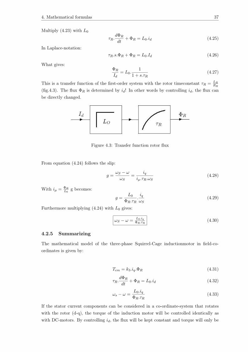
This is a transfer function of the first-order system with the rotor timeconstant τR = LRRR
(fig.4.3). The flux ΦR is determined by id! In other words by controlling id, the flux canbe directly changed.
Figure 4.3: Transfer function rotor flux
From equation (4.24) follows the slip:
g =ωS − ω
ωS=
iqiµ.τR.ωS
(4.28)
With iµ = ΦRL0
g becomes:
g =L0
ΦR.τR.iqωS
(4.29)
Furthermore multiplying (4.24) with L0 gives:
ωS − ω = L0.iqΦR.τR
(4.30)
4.2.5 Summarizing
The mathematical model of the three-phase Squirrel-Cage inductionmotor in field-co-ordinates is given by:
Tem = k3.iq.ΦR (4.31)
τR.dΦR
dt+ ΦR = L0.id (4.32)
ωs − ω =L0.iqΦR.τR
(4.33)
If the stator current components can be considered in a co-ordinate-system that rotateswith the rotor (d-q), the torque of the induction motor will be controlled identically aswith DC-motors. By controlling id, the flux will be kept constant and torque will only be
4. Mathematical formulas 38
influenced by current iq.The speed n/ω of the induction motor can be directed according to (4.33) by influencingωS and iq.
4.3 Field-weakening
Assume an induction motor, that is powered from a converter with, variable voltage (UN )and frequency (fN ).
New parameter(s):
UN = nominal voltage of the converter (=max. voltage) [V ]
fN = nominal frequency of the converter [Hz]
The nominal flux (Φ) of the motor equals [5]:
Φ = k1Unom
f(4.34)
(For example with a 230V-50hz motor: Uf = 230
50 = 4, 6(V/Hz)
New parameter(s)7::
Φ = the magnetical flux [Wb]
U = the voltage given by the frequency-controller [V ]
f = the frequency given by the frequency-controller [Hz]
k1 = a constant [−]
ωb = speed at nominal flux [rad/s]
The speed at nominal flux is called ωb.
To lower the speed of the motor, the frequency has to be changed. From equation (4.34)however it is seen that when lowering the frequency, Φ also changes. To keep the fluxnominal, U has to be linearly proportional with the changing f .
Raising frequency (and in this way also speed) and voltage will only be possible until UN
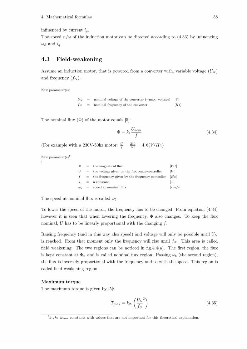
is reached. From that moment only the frequency will rise until fN . This area is calledfield weakening. The two regions can be noticed in fig.4.4(a). The first region, the fluxis kept constant at Φn and is called nominal flux region. Passing ωb (the second region),the flux is inversely proportional with the frequency and so with the speed. This region iscalled field weakening region.
Maximum torqueThe maximum torque is given by [5]:
Tmax = k2.
(US
fS
2)(4.35)
7k1, k2, k3,... constants with values that are not important for this theoretical explanation.

4. Mathematical formulas 39
Figure 4.4: Flux reference as a function of the motor speed. From [7].
In nominal flux region, Uf is kept constant, so the maximum torque keeps the same value.
In the field-weakening region U stays constant and the maximum torque, Tmax = k3f2 , is
square proportional with f .
PowerThe provided power of the motor is given by [5]:
P = ω.T =2.π.n
60.T (4.36)
In Nominal flux region:Φn → P =
2.π.n
60.T = kx.n (4.37)
Since the speed is linearly proportional with f :
P = k4.n = k5.f (4.38)
The power is linearly proportional with f until U = Unom. In field weakening regionT = kz
f , so:
P = ω.T =2.π.n
60.k6
f=
2.π
60.kz.
n
f(4.39)
And because n is proportional with f , P will be constant.
Field weakening and field oriented control
Except in the case of the minimum loss control, the basic control strategy is to operate theinduction machine with constant flux, represented by the magnetizing current iµ, up to thebase speed ωb and at the voltage above the base speed. The variation of the magnetizingcurrent reference required to implement this strategy is shown in fig.4.4(b).At constant flux, the maximum electromagnetic torque is limited by the q-axis currentand thus constant. The operation at constant terminal voltage beyond the base speed iscarried out by reducing the flux reference inversely proportional to the motor speed.
Chapter 5
Field orientated control system:matlab/mathemetical model
5.1 Introduction
Chapter 4 provides a mathematical model which will be used to create a couple of blockschemes to control the torque and (or) the speed of a three-phase Squirrel-Cage inductionmotor. The currents iq and id have to be defined to controle the torque and flux. To definethis fictive currents the magnitude and situation of the rotor flux has to be determined.For this purpose, there are two usual methods [3]:
• direct calculation out of the voltage and current measurement at stator-side. Forthe direct calculation only the motor parameters are needed.
• indirect calculation out of the slip. For the indirect calculation a slip measurementis required with an encoder or a tacho on the motor-shaft and rotor timeconstanthas to be known.
The direct field orientated control is discussed in Appendix C. The more complete indirectfield orientation control is discussed in this chapter.
5.2 Indirect field orientation
5.2.1 Determine situation of ~ΦR
Out of equation 4.33:
ωs − ω =L0.iqΦR.τR
ωS can be determine.Integrating ωS provides the angle λ(t), the angle where ~ΦR is situated in respect to thestator.This calculation is implemented model in matlab is represented in fig.5.1.
40

5. Field orientated control system: matlab/mathemetical model 41
Figure 5.1: Determination of lambda (λ)
5.2.2 Clark-transformation
The determination of iα and iβ is realized by a Clark-transformation (equations (3.3) and(3.4)). For the convenience iα and iβ are repeated here:
iα =32iS1
iβ =√
32× (iS2 − iS3)
With:
iS1 + iS2 + iS3 = 0 ⇒ iS1 + iS2 = −iS3 (5.1)
iα and iβ become:
iα =32iS1 (5.2)
iβ =√
32
(2.iS2 + iS1) (5.3)
It is sufficient to have disposal of two of the three stator currents for a 3/2-transformation1
.
5.2.3 Park-transformation
To get from stator co-ordinates, α− β, to field co-ordinates, d-q, a Park-transformation isused (3.15 and 3.16). For the convenience id and iq are repeated here:
id = iα. cos λ + iβ . sinλ
iq = iβ . cos λ− iα. sinλ (5.4)
13/2: an other term for the Clark-transformation.

5. Field orientated control system: matlab/mathemetical model 42
These expressions implemented in matlab leads to fig.5.2.
Figure 5.2: Block scheme of the vector rotator (Park-transformation)
A vector in the α−β system has to be multiplied by e−jλ to go to the d-q reference frame,therefore e−jλ is the symbolic representation of the vector rotator.
Inverse Park-transformationThe inverse Park-transformation is given by (3.17) and (3.18) and is used to get from field-co-ordinates to stator-co-ordinates. Similar as with the Park-transformation, the symbolicrepresentation is given by ejλ.
5.2.4 Block scheme for an indirect field orientation
The mathematical formulas ((4.31), (4.32) and (4.33)) make that the amplitude and fre-quency of the injected stator current can be defined. However the rotor speed (or slip) isneeded, for this a tacho is used.Further the rotor speed constant plays an important roll in the accuracy of the systembecause τR depends on the temperature and air-gap flux.Fig.5.3 shows the total block scheme to calculate ΦR and λ out of stator current and rotorspeed (or position) of the rotor.
Notice three parts on the figure:
1. On the left iS1 and iS2 , to determine iα and iβ : 3/2 transformation (section 5.2.2)
2. In the middle the Park-transformation, to get id and iq. (section 5.2.3)
3. On the right bottom the determination of angle λ(t) (section 5.2.1)
Furthermore out equations (C.1) and (C.3) follows:

5. Field orientated control system: matlab/mathemetical model 43
Figure 5.3: Full block scheme of the counting module
d( ~ΦR.ej.δ)dt
=LR
L0.
[~uS(t)−RS . ~iS − σ.LS .
d~iSdt
]d( ~ΦR.ej.δ)
dt= RS .
LR
L0.
[~uS(t)RS
− . ~iS − σ.τS .d~iSdt
](5.5)
with:
τS = LSL0
Stator − time− constant
Equation 5.5 is given in stator-co-ordinates and allows to determine the amplitude andfrequency of the needed stator voltage.
5.3 Field oriented control: block scheme
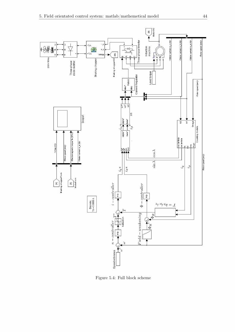
Finally the blocks scheme with relating PI-controllers for the field oriented speed regulatorof an inductionmotor with forced stator currents (fig.5.4). The parameters used for themotor specifications are found in appendix D.
5. Field orientated control system: matlab/mathemetical model 44
Figure 5.4: Full block scheme
5. Field orientated control system: matlab/mathemetical model 45
5.4 Process of work
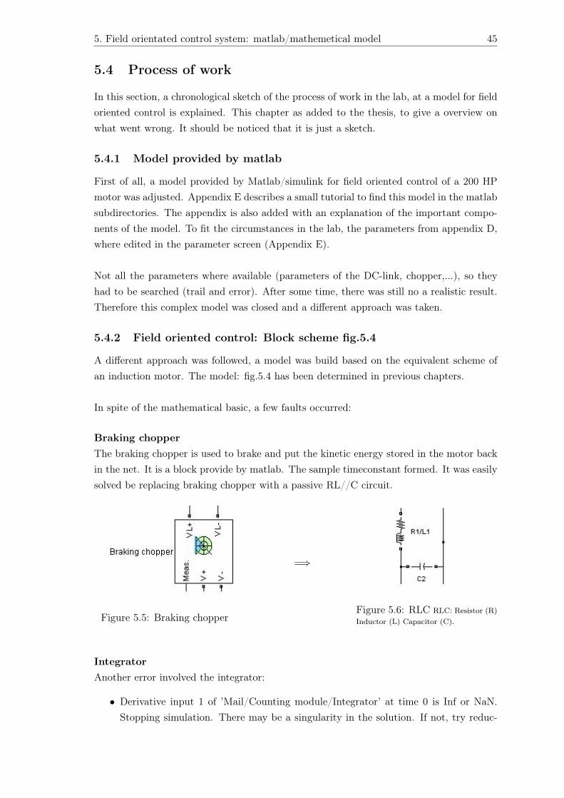
In this section, a chronological sketch of the process of work in the lab, at a model for fieldoriented control is explained. This chapter as added to the thesis, to give a overview onwhat went wrong. It should be noticed that it is just a sketch.
5.4.1 Model provided by matlab
First of all, a model provided by Matlab/simulink for field oriented control of a 200 HPmotor was adjusted. Appendix E describes a small tutorial to find this model in the matlabsubdirectories. The appendix is also added with an explanation of the important compo-nents of the model. To fit the circumstances in the lab, the parameters from appendix D,where edited in the parameter screen (Appendix E).
Not all the parameters where available (parameters of the DC-link, chopper,...), so theyhad to be searched (trail and error). After some time, there was still no a realistic result.Therefore this complex model was closed and a different approach was taken.
5.4.2 Field oriented control: Block scheme fig.5.4
A different approach was followed, a model was build based on the equivalent scheme ofan induction motor. The model: fig.5.4 has been determined in previous chapters.
In spite of the mathematical basic, a few faults occurred:
Braking chopperThe braking chopper is used to brake and put the kinetic energy stored in the motor backin the net. It is a block provide by matlab. The sample timeconstant formed. It was easilysolved be replacing braking chopper with a passive RL//C circuit.
Figure 5.5: Braking chopper
=⇒
Figure 5.6: RLC RLC: Resistor (R)Inductor (L) Capacitor (C).
IntegratorAnother error involved the integrator:
• Derivative input 1 of ’Mail/Counting module/Integrator’ at time 0 is Inf or NaN.Stopping simulation. There may be a singularity in the solution. If not, try reduc-

5. Field orientated control system: matlab/mathemetical model 46
ing the step size (either by reducing the fixed step size or by tightening the errortolerances).
Figure 5.7: Derivative input 1
The first thing that was tried was reducing the fixed step size in any way. Reducing thestep size did not help. The following step was a search at the internet to find variousanswers. There was nothing found that could solve the error. Another path had to befollowed to find the solution.
5.4.3 Basic model
A basic model (fig.5.8) was the ground for the next step. This is a simplified model wherethe d and q current can be controlled directly.

5. Field orientated control system: matlab/mathemetical model 47
Figure 5.8: Basic scheme of field oriented control of an AC-motor. From [8].
The following scheme was builded in simulink (fig.5.9):
Figure 5.9: Basic model

5. Field orientated control system: matlab/mathemetical model 48
It should be noticed that the counting module block (fig.5.3) is changed. The angle wasdirectly derived from the motor (the motor model provided by matlab gives some param-eters for the use of the simulink model writer). In this way the fault (Derivative input 1)was avoided. This idee was later on also tested on the previous scheme (fig.5.4).Another change was adding memory blocks. They put a small delay on the feedback signal.So another fault that occurred could be eliminated.The following output was found:
Figure 5.10: Basic output. blue: torque, red: current and green: speed.
Fig.5.10 shows the torque, speed and currents. It is an output that does not fit to realitybut it helped the writer of this thesis to learn more about simulink. It could provide asolution for the problem(s) experienced with the block scheme in section 5.4.2.
5.4.4 Φ model
In the mean time, a different model was implemented in matlab. It is based on the resultsof a study performed by Dr. Vásárhelyi Joszef (University of Miskolc).

5. Field orientated control system: matlab/mathemetical model 49
Figure 5.11: Φ-scheme (Φ: flux).
The name of fig.5.11 is based on the use of the flux Φ in the feedback. The counting moduleblock is changed inside with a circuit based the on following formulas:
Φ =√
Φ2Sd + Φ2
Sq (5.6)
cos λ =Φ2
Sd
Φ(5.7)
sinλ =Φ2
Sq
Φ(5.8)
A second feedback is added, the speed. The model also has an output. But the questionis if the output of the basic model and the Φ model are (nearly) correct. Because themathematical basic, on which this model is based, is not known by the author of thisthesis.
5.4.5 Updated model
The last model that was builded is the first, fig.5.4, with some applied changes. Thesechanges are based on what was learned while investigating the basic and Φ models in thelatest paragraph’s (fig.5.12).

5. Field orientated control system: matlab/mathemetical model 50
Figure 5.12: Final model
Another fault occurred: The programme showed an output but the scope did not show thewhole output only the last couple of ms. By this, the courage and time to do this labwork

5. Field orientated control system: matlab/mathemetical model 51
started to shrink.
5.4.6 final matlab model
The last model that was tried, is one provide by matlab in the demo section (fig.5.13):
Figure 5.13: Vector control of a variable-frequency induction motor drive
The vector control block has the same mathematical basic as explained in chapters 2,3and 4. This model should be able to provide a good output to compare to the reality.Optimizing the parameters should do the trick. The fact that it was not able anymore totest the model in reality lead to the cancelation of the optimization of the block.
Chapter 6
Field oriented control scheme for amulti-phase induction motor
6.1 Introduction
Three-phase induction motors are presently a standard for industrial electrical drives. Rel-atively low cost, high reliability, robustness and maintenance-free operation are among thereasons three-phase induction drives are replacing DC-drive systems. The development ofpower electronics and signal processing systems has eliminated what had been one of thegreatest disadvantages of AC-systems, that is, the issue of control. With modern tech-niques of field oriented control, variable speed control of induction machines is readilyachievable. But the desire to improve the performance even more, motivates the use ofmotors with a phase number higher then three: multi-phase motors.
This chapter is a analyze of literature (articles), the basics of the multi-phase motor isdiscussed and the link to field oriented control is made.
6.2 Multi-phase motor basics
The basic concept of an AC-multi-phase motor is simple. Instead of one set of three-phasewindings, the motor has two ore more. Each of these windings are spatially shifted inrespect to each other. The most commonly discussed in literature is by far the six-phasemotor([9], [10]). The spatial distance between the two three-phase windings1 of the six-phase can be 0, 30 and 60 electrical degrees. A visual thought, duplicating the three-phasewindings of a motor and rotating these duplicat along stator-side. When the displacementis 30 it is called an asymmetric six-phase induction motor. The 60 displacement is calleda symmetric six-phase induction motor. The two motors are represented in fig.6.1(a) and(b).
1The two three-phase windings: this is the same as two sets of three-phase windings.
52

6. Field oriented control scheme for a multi-phase induction motor 53
(a) asymmetric (b) Symmetric
Figure 6.1: Stator windings of a six-phase asynchrone motor
BenefitsMulti-phase motors posses several advantages over the conventional three-phase motor es-pecially for high-power applications. For these applications, high-power and high-switching-frequency semiconductor devices are very expensive or even not available. For these cases,with multi-phase motors, the controlled power can be divided among more inverter legs toreduce the load on one inverter. This instead of the need of parallel techniques.Other potential advantages of the multi-phase drives over the conventional three-phasessystem are:
• It is possible to smooth the torque pulsations
• The rotor harmonic losses can be reduced
• It is possible to reduce the harmonic content of the DC-link current
• The overall system reliability, which is very important for high-power drives, is im-proved in case of the loss of one motor-phase
• Having additional phases gives more degrees of freedom
• Higher/improved reliability, so smaller fault tolerance is possible
It was concluded in the article with reference [11] that, in the case of a six-phase induc-tion motor, it is an advantage to use an asymmetrical stator winding structure. With twothree-phase windings spatially shifted by 30, instead of a symmetrical winding structurewith a 60 spatial shift between any two consecutive phases. The background idea behindthis conclusion is related to the pre-PWM era of VSI control, when 180 conduction modewas utilized. By using an asymmetrical six-phase motor, it became possible to eliminate

6. Field oriented control scheme for a multi-phase induction motor 54
the sixth harmonic torque pulsation from the torque ripple and also significantly reducesthe rotor losses by reducing the rotor current harmonic components. By this (almost) alldiscussed work/literauur considers the asymmetric six-phase AC-motor. From the veryfew articles found linked to the symmetrical, the article [12] is word mentioning. Therefield oriented control of a symmetric six-phase induction motor is discussed.Next to all the benefits, the are also some downsizes. E.g. the current control is a problembecause of the unbalanced current sharing between the two three-phase sets, due to thesmall asymmetries that cannot be eliminated. But a more important disadvantage are theharmonics, that is why al lot of work considers techniques to improve the harmonic dis-tortion e.g. [13]. Others use harmonic injection to improve the induction motor behaviour[14]. Another solution to this problem is the use of an appropriate PWM technique withoutmodifying the motor design and construction [15].
ConceptThe induction machine can be split up in:
• Split-phase
• Dual three-phase
• Double star
With split-phase induction motors2, the sixth harmonic torque pulsation can be eliminated.Also, air-gap flux created by fifth and seventh harmonic currents in a high-power six-stepconverter-fed system is dramatically reduced with the downside of increased converter har-monic currents. PWM (pulse width modulation) techniques are employed to overcome thisproblem by eliminating the harmonic currents in the modulation process when the powerratings are not prohibitive [16],[14].Dual-stator motors are similar to split-phase machines with the difference that the statorgroups are not necessarily equal. A dual-stator machine with different numbers of polesin each three-phase group has been proposed to obtain controllability at low speeds. Twoindependent stator windings are used for an induction generator system. One set of wind-ings is responsible for the electromechanical power conversion, while the second one is usedfor excitation purposes. A PWM converter is connected to the excitation windings andthe load is connected directly to the power windings[14].The rotor of the split-phase and dual three-phase are short-circuited along the six rotorends, to form one starpoint which is mostly isolated (no neutral). With the double star,the two different three-phase sets are separately fixed in two starpoints. The mean reasonto choose for a double star is the ability of connection to two different starpoints and soone variable less and the abilities to have more control on harmonic injection[14].Fig.6.2 shows the split-phase or dual-stator motor.
2In this context a asymmetrical six-phase motor is considered from now.

6. Field oriented control scheme for a multi-phase induction motor 55
Figure 6.2: Split/dual three-phase induction motor. From [17].
6.3 Model of the six-phase induction motor
A schematic representation of the stator and rotor windings for a six-phase induction motor(fig.6.2) is given in fig.6.3. The six stator-phases are divided into two wye-connected three-phase sets, abc and xyz, who are displaced by an angle α = 30. The windings of eachthree-phase set are uniformly distributed and have axis that are displaced 120 in respect toeach other. The three-phase rotor windings ar, br and cr are also sinusoidally distributed3.
The six-phase induction motor is a six-dimensional system. Therefore, modeling and con-trol of this motor in the original reference frame would be very difficult. For this reason,it is necessary to obtain a simplified model to control this type of motor. To derive themotor model, some simplification are being considered:
• The windings are sinusoidally distributed and the rotor-cage is equivalent to a six-phase wound rotor.
• The magnetic saturation, the mutual leakage inductances and the core losses areneglected.
The voltage equations4 in the original phase co-ordinates can be described as in the articles
3It should be noticed that in fig.6.3 xr, yr and zr are not displayed to keep a more clear overview inthe figure. It can be easily visualized that there is a angle of 30 between ar and the place where xr issituated.
4-Notice the similarity with equations 2.18 and 2.21.-Because the motormodel is more complexity then in chapter 2 a matrix is used to give an easieroverview.
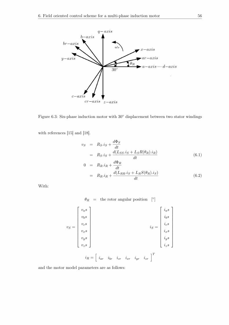
6. Field oriented control scheme for a multi-phase induction motor 56
Figure 6.3: Six-phase induction motor with 30 displacement between two stator windings
with references [15] and [18].
vS = RS .iS +dΦS
dt
= RS .iS +d(LSS .iS + LSR(θR).iR)
dt(6.1)
0 = RR.iR +dΦR
dt
= RR.iR +d(LRR.iS + LRS(θR).iS)
dt(6.2)
With:
θR = the rotor angular position []
vS =
vas
vbs
vcs
vxs
vys
vzs
iS =
ias
ibs
ics
ixs
iys
izs
iR =
[iar ibr icr ixr iyr izr
]Tand the motor model parameters are as follows:
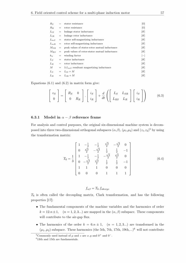
6. Field oriented control scheme for a multi-phase induction motor 57
RS = stator resistance [Ω]
RR = rotor resistance [Ω]
LlS = leakage stator inductance [H]
LlR = leakage rotor inductance [H]
LmS = stator self-magnetizing inductance [H]
LmR = rotor self-magnetizing inductance [H]
MSR = peak values of stator-rotor mutual inductance [H]
MRS = peak values of rotor-stator mutual inductance [H]
kw = winding factor [−]
LS = stator inductance [H]
LR = rotor inductance [H]
M = 3.LmS resultant magnetizing inductance [H]
LS = LlS + M [H]
LR = LlR + M [H]
Equations (6.1) and (6.2) in matrix form give: vS
0
=
RS 0
0 RR
.
iS
iR
+d
dt
LS LSR
LRS LR
iS
iR
(6.3)
6.3.1 Model in α− β reference frame
For analysis and control purposes, the original six-dimensional machine system is decom-posed into three two-dimensional orthogonal subspaces (α,β), (µ1,µ2) and (z1,z2)5 by usingthe transformation matrix:
T6 =13
1 −12 −1
2
√3
2 −√
32 0
0√
32 −
√3
212
12 −1
1 −12 −1
2 −√
32
√3
2 0
0 −√
32
√3
212
12 −1
1 1 1 0 0 0
0 0 0 1 1 1
(6.4)
fαβ = T6.fabcxyz
T6 is often called the decoupling matrix, Clark transformation, and has the followingproperties [17]:
• The fundamental components of the machine variables and the harmonics of orderk = 12.n± 1, (n = 1, 2, 3...) are mapped in the (α, β) subspace. These componentswill contribute to the air-gap flux.
• The harmonics of the order k = 6.n ± 1, (n = 1, 2, 3...) are transformed in the(µ1, µ2) subspace. These harmonics (the 5th, 7th, 17th, 19th,...)6 will not contribute
5Commonly used instead of µ and z are x, y and 0+ and 0−.613th and 15th are fundamentals.

6. Field oriented control scheme for a multi-phase induction motor 58
to the air-gap flux because the (α, β) and (µ1, µ2) subspaces are orthogonal.
• The zero-sequence components are mapped in the (z1, z2) subspace.
In other words the flux/torque producing stator currents are linked with the α−β currentcomponents, while the µ1 − µ2 and z1 − z2 are non-air-gap flux/torque producing statorcurrents. Further since the rotor is short circuited, µ1 − µ2 and z1 − z2 cannot exist [19].It should be noticed that the used matrix equation (6.4) is not power invariant because itis not orthogonal. On the other hand, in case of sinusoidal quantities, this transformationmatrix is amplitude invariant. For this reason it is preferred to use this transformationmatrix to obtain the motor model. Thus, applying the transformation (6.4) to the voltageequations (6.1) and (6.2):
[T6].[vS ] = [T6].RS .[T−6 1].[T6].[iS ]
+d
dt([T6].[LSS ].[T−
6 1].[T6].[iS ] + [T6].[LSR.[T−6 1].[T6].[iR]) (6.5)
0 = [T6].[RS ].[T−6 1].[T6].[iR]
+d
dt([T6].[LRR].[T−
6 1].[T6].[iR] + [T6].[LRS ].[T−6 1].[T6].[iS ]) (6.6)
Where the voltage and current vectors in the new reference frame are:
[T6].[vS ] = [vsα vsβ vsµ1 vsµ2 vsz1 vsz2 ]t (6.7)
[T6].[iS ] = [isα isβ isµ1 isµ2 isz1 isz2 ]t (6.8)
[T6].[iR] = [irα irβ irµ1 irµ2 irz1 irz2 ]t (6.9)
[RS ] = RS .I6, [RR] = RR.I6 with: I6 is the 6x6 identity matrix. (6.10)
[LSS ] = LlS .I6 + LmS .
1 −12 −1
2
√3
2 −√
32 0
−12 1 −1
2 0√
32 −
√3
2
−12 −1
2 1 −√
32 0
√3
2√3
2 0 −√
32 1 −1
212
−√
32
√3
2 0 −12 1 1
2
0 −√
32
√3
2 −12 −1
2 1
(6.11)
[LRR] = LlR.I6 + LmR.
1 −12 −1
2
√3
2 −√
32 0
−12 1 −1
2 0√
32 −
√3
2
−12 −1
2 1 −√
32 0
√3
2√3
2 0 −√
32 1 −1
212
−√
32
√3
2 0 −12 1 1
2
0 −√
32
√3
2 −12 −1
2 1
(6.12)
[LSR(θR)] = MSR.[θ]SR, [LRS(θR)] = MSR.kw.[θ]RS (6.13)

6. Field oriented control scheme for a multi-phase induction motor 59
With:
[θ]SR =
cosθ1 cosθ2 cosθ3 cosθ4 cosθ5 cosθ6
cosθ3 cosθ1 cosθ2 cosθ6 cosθ4 cosθ5
cosθ2 cosθ3 cosθ1 cosθ5 cosθ6 cosθ4
cosθ4 cosθ5 cosθ6 cosθ1 cosθ2 cosθ3
cosθ6 cosθ4 cosθ5 cosθ3 cosθ1 cosθ2
cosθ5 cosθ6 cosθ4 cosθ2 cosθ3 cosθ1
(6.14)
and:
[θ]RS =
cosθ1 cosθ3 cosθ2 cosθ7 cosθ8 cosθ9
cosθ2 cosθ1 cosθ3 cosθ9 cosθ7 cosθ8
cosθ3 cosθ2 cosθ1 cosθ8 cosθ6 cosθ7
cosθ4 cosθ6 cosθ5 cosθ1 cosθ3 cosθ2
cosθ5 cosθ4 cosθ6 cosθ2 cosθ1 cosθ3
cosθ6 cosθ5 cosθ4 cosθ3 cosθ2 cosθ1
(6.15)
θ1 = θR, θ2 = θR +4.π
6, θ3 = θR +
8.π
6
θ4 = θR +π
6, θ5 = θR +
5.π
6, θ6 = θR −
π
2
θ7 = −θR +π
6, θ8 = −θR +
5.π
6, θ9 = −θR −
π
2
Application these, articles [15] and [18], leads to three sets of decoupled equations, corre-sponding to the three subspaces (α,β),(µ1,µ2) and (z1,z2):
Motor model in (α, β) subspacevsα
vsβ
0
0
=
RS + dLS
dt 0 dMdt 0
0 RS + dLSdt 0 dM
dt
dMdt ωR.M RR + dLR
dt ωR.LR
−ωR.M dMdt −ωR.LR RR + dLR
dt
.[isα isβ irα irβ]t
(6.16)The (α, β) motor model is similar to the three-phase motor model in the stationary refer-ence frame (section 3).
Motor model in (µ1, µ2) subspace
vSµ1
vSµ2
=
RS + dLlSdt 0
0 RS + dLlSdt
.
iSµ1
iSµ2
(6.17)
(6.18)

6. Field oriented control scheme for a multi-phase induction motor 60
Motor model in (z1, z2) subspace
vSz1
vSz2
=
RS + dLlSdt 0
0 RS + dLlSdt
.
iSz1
iSz2
(6.19)
(6.20)
Equation (6.16),(6.17) and (6.16) leads to the equivalent scheme fig.6.4.
Figure 6.4: Single-phase equivalent circuits of the motor. From [19].
Stator voltage equations (vSα,µ1,z1 and vSβ,µ2,z2) show that it is not sufficient to controlonly two flux/torque producing stator current components. If the inverter produces suchvoltages that µ1 − µ2 stator voltage components exist (there are voltage harmonics of theorder 6n±1 (n=1,3,5...)), stator current µ1−µ2 component will flow freely. Further, sincethere is only one star point, the z component of the stator current can flow freely as wellif the inverter produces harmonics of the order 3n. There are therefore five independentcurrents (this can be reduced to four, by disconnecting the star points of the two three-phase windings, since the z component of the stator current then cannot flow.). Thisproblem can be overcome for asymmetric six-phase motors with isolated star points byusing two pairs of stationary current controllers (α, β) and (µ1, µ2) as in [20].
6.3.2 Model in d− q reference frame
To go to field oriented control a rotational transformation is applied. For a six-phase motorthis is in the following form:

6. Field oriented control scheme for a multi-phase induction motor 61
dq6 =
cosθ sinθ 0 0 0 0
−sinθ cosθ 0 0 0 0
0 0 1 0 0 0
0 0 0 1 0 0
0 0 0 0 1 0
0 0 0 0 0 1
(6.21)
The link between the reference frame is fdq = dq6.fαβ . Notice the similarity with thethree-phase diversion (equation (3.5.1)). In fact the three-phase diversion is derived fromthe same basic as the six-phase or any n-phase motor. The only difference is the size ofthe identity matrix. [1x1] for the three-phase, [4x4] for the six-phase motor.In 3.5.1 it was silent accepted that only a [2x2] matrix is used and the added [1x1] identitymatrix was not considered. This is however because the zero-component is required neitherfor motor control nor for describing the dynamic motor behaviour. A more expandedexplanation on this is given in [7], more explanation on controle of a n-phase motor ingeneral is given in [21].
6.4 Field oriented control of a multi-phase motor
Section 6.3 shows that the field oriented control of a multi-phase induction motor is basedon the same fundamentals as three-phase field oriented control. The only difference is theClark transformation and the inverse Clark transformation. Where in general a matrix(Tn)is used to represent the linkage.Fig.6.5 shows the basic model of field oriented control for a six-phase induction motor. Thismodel is the starting point to expend in more sophisticated models similar to three-phase.
Figure 6.5: Basic six-phase model for field oriented control. From [17].
The model in fig.6.5 is very simple but it is not able to compensate asymmetries of thedrive. Thus, due to small asymmetries in the stator windings and supply voltages, thetwo sets of three-phase stator currents have rather different amplitudes depending on theoperating/practical conditions. For this reason, alternative directions of thoughts have to

6. Field oriented control scheme for a multi-phase induction motor 62
be used. In literature a different distraction based on the rotating reference frame [22] isexcellent for field oriented control.
6.4.1 Field oriented control in the rotating reference frame
Differently then in section 6.3. It is assumed that:
• There is a mutual leakage inductances
• There is no physical fault propagation from one three-phase set to the other three-phase set as the neutral of both stator winding sets is separated7
• The two winding sets have different parameters
The following voltage equations are written for a multi-phase motor[22]:
vq1 = R1.iq1 + ωK .Φd1 +dΦq1
dt(6.22)
vd1 = R1.id1 − ωK .Φq1 +dΦd1
dt(6.23)
vq2 = R2.iq2 + ωK .Φd2 +dΦq2
dt(6.24)
vd2 = R2.id2 − ωK .Φq2 +dΦd2
dt(6.25)
0 = RR.iqR + (ωK − ωR)ΦdR +dΦqR
dt(6.26)
0 = RR.idR − (ωK − ωR)ΦqR +dΦdR
dt(6.27)
Here ωK is the speed of the reference frame, the rotor quantities are referred to the statorand the expressions for stator and rotor flux linkages are:
Φq1 = Ll1.iq1 + Llm′(iq1 + iq2)− Lldq′.id2 + Lm(iq1 + iq2 + iqR) (6.28)
Φd1 = Ll1.id1 + Llm′(id1 + id2) + Lldq′.iq2 + Lm(id1 + id2 + idR) (6.29)
Φq2 = Ll2.iq2 + Llm′(iq1 + iq2) + Lldq′.id1 + Lm(iq1 + iq2 + iqR) (6.30)
Φd2 = Ll2.id2 + Llm′(id1 + id2)− Lldq′.iq1 + Lm(id1 + id2 + idR) (6.31)
ΦqR = LlR.iqR + Lm(iq1 + iq2 + iqR) (6.32)
ΦdR = LlR.idR + Lm(id1 + id2 + idR) (6.33)
LlM ′ = kw.LlM and Lldq′ = kw2.Lldq (6.34)
7Joint neutrals give larger torque.
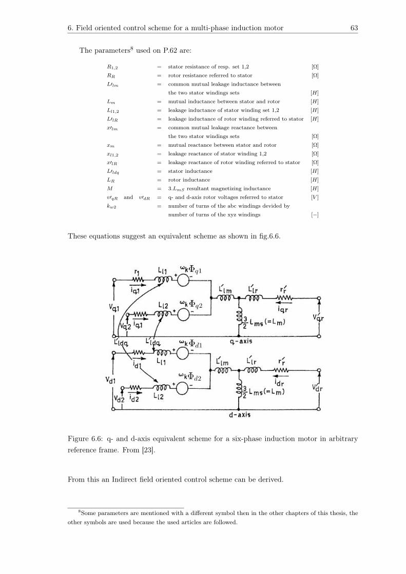
6. Field oriented control scheme for a multi-phase induction motor 63
The parameters8 used on P.62 are:
R1,2 = stator resistance of resp. set 1,2 [Ω]
RR = rotor resistance referred to stator [Ω]
L′lm = common mutual leakage inductance between
the two stator windings sets [H]
Lm = mutual inductance between stator and rotor [H]
Ll1,2 = leakage inductance of stator winding set 1,2 [H]
L′lR = leakage inductance of rotor winding referred to stator [H]
x′lm = common mutual leakage reactance between
the two stator windings sets [Ω]
xm = mutual reactance between stator and rotor [Ω]
xl1,2 = leakage reactance of stator winding 1,2 [Ω]
x′lR = leakage reactance of rotor winding referred to stator [Ω]
L′ldq = stator inductance [H]
LR = rotor inductance [H]
M = 3.LmS resultant magnetizing inductance [H]
v′qR and v′dR = q- and d-axis rotor voltages referred to stator [V ]
kw2 = number of turns of the abc windings devided by
number of turns of the xyz windings [−]
These equations suggest an equivalent scheme as shown in fig.6.6.
Figure 6.6: q- and d-axis equivalent scheme for a six-phase induction motor in arbitraryreference frame. From [23].
From this an Indirect field oriented control scheme can be derived.
8Some parameters are mentioned with a different symbol then in the other chapters of this thesis, theother symbols are used because the used articles are followed.

6. Field oriented control scheme for a multi-phase induction motor 64
6.4.2 Derivation of indirect field oriented control scheme
The indirect field oriented control scheme is derived from the dynamic equations of themotor in synchronously rotating reference frame9 [23]. The rotor voltage equations aregiven by (6.26) and (6.27):
0 = RR.iqR + (ωK − ωR)ΦdR +dΦqR
dt
0 = RR.idR − (ωK − ωR)ΦqR +dΦdR
dt
The resultant rotor flux ΦR, also known as the rotor flux-linkages phasor, is assumedto be on the d axis, which corresponds with the reality, that the rotor flux linkagesare one single variable. Hence, aligning the d-axis with the rotor flux phasor yields
ΦR = ΦdR (6.35)
ΦqR = 0 (6.36)dΦR
dt= 0 (6.37)
and ωsl = ωk − ωr (6.38)
Substituting (6.35-6.38) in (6.26) and (6.27):
RR.iqR + ωsl.Φr = 0 (6.39)
RR.idr +dΦR
dt= 0 (6.40)
The rotor currents in terms of the stator currents are derived from (6.32 and 6.33):
iqR = −(
LM
LR
).(iq1 + iq2) (6.41)
idR =(
ΦR
LR
)−(
LM
LR
).(id1 + id2) (6.42)
Substituting this in 6.39 and 6.40 leads to:
if =(
1Lm
).[1 +
dTR
dt].ΦR (6.43)
ωsl =(
Lm
TR
).
(iTΦR
)(6.44)
Where:
if = (id1 + id2 (6.45)
iT = (iq1 + iq2 (6.46)
TR =LR
RR(6.47)
It seems that new d- and q-axis currents occur as flux-producing (if ) and torque-producing(iT ) components of the stator current phasor, respectively. TR denotes the rotor timecon-stant.
9d-q reference frame.

6. Field oriented control scheme for a multi-phase induction motor 65
Similar as in chapter 3, the electromagnetic torque is derived as
T = K.ΦR.iT (6.48)
With:K =
(32
).(
P2
).(
LmLR
)From all the derivations above, it can be concluded that the implementation of the fieldoriented control scheme is very similar as with the three-phase induction motor.

Chapter 7
Conclusion and further investigation
7.1 Conclusion
Three-phase induction motors have a long history. These motors play an important, dailyrole in many industria branches. That is why a good control system for the three-phasemotor is indispensable.In a non steady state situation, the control of the three-phase induction motor is simplifiedby changing to different reference frames. The torque and the speed of the induction motorare controlled similar to the DC-motor by two currents, id and iq. These currents are re-ferred to a reference frame, that is rotating along with the rotor flux (ΦR). This referenceframe is called the d − q reference frame (also called the rotation reference frame). Withthe two currents (id and iq), control of a three-phase induction motor becomes very easily.This type of control is called field oriented control.The need to keep improving leaded to the use of multi-phase induction motors, they haveseveral benefits over the standard three-phase motors. Furthermore the control of multi-phase motors is available by the same control system as with three-phase induction motors:field oriented control of multi-phase motors.
7.2 Further investigation
Because of a lack of time, the implementation of a field control system in matlab was notfinished. The implementation of a working model would be the next step for this thesis.Furthermore, the subject multi-phase motors is still not very well known in literature.Further investigation should focus on the application and control of multi-phase motors tomake it as a standard for industria.
66

Bibliography
1. http://users.skynet.be/kevin.vangenechten/driefasige%20asynchrone%20motor.pdf.
2. http://en.wikipedia.org/wiki/Electric_motor/.
3. J. Pollefliet. Elektronische Vermogencontrole 2. Elektronische motorcontrole. J. Story-Scientia bvba Wetenschappelijke Boekhandel, Gent, 2004. (in dutch).
4. Th. Wildi. Electrical Machines, Drives, and Power Systems. Pearson Education In-ternational, 2002.
5. G. R. Slemon. Electric Machines and Drives. Addison-Wesley Publisching Co, Toronto,1992.
6. P. C. Sen. Principles of Electric Machines and Power Electronics. John Wiley andSons, NewYork–Toronto–Singapore–Chichester–Brisbane, 1989.
7. J. Driesen, G. Terörde, and R. Belmans. Introduction to AC Drives. K.U Leuven-ESAT-ELECTA.
8. Texas InstrumentsEurope. Field Orientated Control of 3-Phase AC-Motors.http://focus.ti.com/lit/an/bpra073/bpra073.pdf, 24:0–24, 1998.
9. A. R. Bakhshai, G. Joos, and H. Jin. Space vector PWM control of a split-phaseinduction machine using the vector classification technique, 1998.
10. A. Munoz and T. A. Lipo. Dual stator winding induction machine drive. IEEE Trans.Ind. Applicat, 36:1369–1379, 2000.
11. R. H. Nelson and P.C. Krause. Induction machine analysis for arbitrary displacementbetween multiple winding sets. IEEE Trans. Power Apparatus, PAS-93:841–848, 1974.
12. S. N. Vukasavic, M. Jones, E. Levi, and J. Varga. Rotor flux oriented control of asymmectrical six-phase induction machine. Electric Power Systems Research, 75:142–152, 2005.
13. L. Xu and L. Ye. Analysis of a novel stator winding structure minimizing harmoniccurrent and torque ripple for dual six-step converter-fed high power ac machine drives.IEEE Trans. Ind. Applicat., 31:84–90, 1995.
67

. BIBLIOGRAPHY 68
14. R. O. C. Lyra and Thomas A. Lipo. Torque Density Improvement in a Six-PhaseInduction Motor With Third Harmonic Current Injection. IEEE Transactions OnIndustry Applications, 38:1351–1360, 2002.
15. Y. Zhao and T. A. Lipo. Space vector PWM control of dual three-phase inductionmachine using vector space decomposition. IEEE Trans. Ind. Applicat., 31:1100–1108,1995.
16. K. K. Mohapatra, R. S. Kanchan, M. R. Baiju, P. N. Tekwani, and K. Gopakumar.Independent Field-Oriented Control of Two Split-Phase Induction Motors From aSingle Six-Phase Inverter. IEEE Transactions On Industry Electronics, 52:1372–1382,2005.
17. R. Bojoi, M. Lazzari, F. Profumo, and A. Tenconi. Digital Field-Oriented Controlfor Dual Three-Phase Induction Motor Drives. IEEE Trans. Ind. Applicat, 3:752–760,2003.
18. D. Hadiouche, H. Razik, and A. Rezzoug. Modeling of a double star induction motorfor space vector PWM control. ICEM, pages 392–396, 2000.
19. R. Bojoi, F. Farina, Giovanni Griva, A. Tenconi, and F. Profumo. Direct TorqueControl for Dual Three-Phase Induction Motor Drives. IEEE Transactions On IndustryApplications, 41, 2005.
20. R. Bojoi, F. Farina, A. Tenconi, F. Profumo, and E. Levi. Stationary frame digitalcurrent regulation for dual-three phase induction motor drives. Proceedings of IEEEPower Electronics Specialists Conference PESC, pages 2121–2127, 2004.
21. E. Levi, M. Jones, and S.N. Vukosavic. Even-phase multi-motor vector controlled drivewith single inverter supply and series connection of stator windings. IEE Proc.-Electr.Power Appl., 150(5):580–590, 2003.
22. G.K. Singh, V. Pant, and Y.P Singh. Voltage source inverter driven multi-phaseinduction machine. Computers and Electrical Engineering, 29:813–834, 2003.
23. G. K. Singh, K. Nam, and S. K. Lim. A Simple Indirect Field-Oriented ControlScheme for Multiphase Induction Machine. IEEE Transactions on industrial electron-ics, 52(4):1177–1184, 2005.
24. http://technosoftmotion.com.

Appendix A
Theoretical Law’s
Appendix made with the book [4].
A.1 Faraday’s law of electromagnetic induction
The law of Faraday reveals the fundamental relationship between the voltage and flux ina circuit. Faraday’s law states:
1. If the flux linking a loop varies as a function of time, a voltage is induced between itsterminals.
2. The value of the induced voltage is proportional to the rate of change of flux.
By definition and according to the SI system of units, when the flux inside a loopvaries at the rate of 1 weber per second, a voltage of 1 V is induced between its termi-nals. Consequently, if the flux varies inside a coil of N turns, the voltage induced is given by:
E = N.∆Φ∆t
(A.1)
With:E = induced voltage [V ]
N = number of turns in the coil [−]
∆Φ = change of flux inside the coil [Wb]
∆t = time interval during which the flux changes [s]
A.2 Voltage induced in a conductor
In many motors and generators, the coils move in respect to a flux that is fixed in space.The relative motion produces a change in the flux linking the coils and, consequently, avoltage is induced according to Faraday’s law. However, in this special case, it is easier tocalculate the induced voltage with reference to the conductors, rather than with referenceto the coil itself. In effect, whenever a conductor cuts a magnetic field, a voltage is induced
69
A. Theoretical Law’s 70
across its terminals. The value of the induced voltage is given by:
E = Blv (A.2)
With:
E = induced voltage [V ]
B = flux density [T ]
l = active length of the conductor in the magnetic field [m]
v = relative speed of the conductor [m/s]
A.3 Lorentz force on a conductor
When a current-carrying conductor is placed in a magnetic field, it is subjected to aforce which is called electromagnetic force, or Lorentz force. This force is of fundamentalimportance because it constitutes the basis of operation of motors, of generators, and manyelectrical instruments.The force acting on a straight conductor is given by:
F = BlI. sin δ2 (A.3)
With:F = force acting in the conductor [N ]
B = flux density [T ]
l = active length of the conductor in the magnetic field [m]
I = current in the conductor [A]
δ2 = angle between the flux and the current []
A.4 Law of Ferraris
Law of Ferraris states the speed of the motor.
ns =60.fs
p(A.4)
fS = netfrequency of the stator inductance [Hz]
p = number of polepares [−]
ns = the synchrone speed [rpm]
Appendix B
Power invariance, iα and iβ
The variables in the α-β-reference frame are no real values, they are fictitious values, prefer-ably describing the real electrical and dynamic behaviour of the machine. Obviously, theoriginal current phasor can be equally described by two other perpendicular vector compo-nents multiplied by a constant scaling factor. According to , the power in the α-β-referenceframe reduced by the scaling factor 2/3 guarantees power invariance. At first sight, thisscaling factor can be distributed on the α-β-current and voltages in different ways, e.g.the α-β- current remains and the voltages α,β are reduced by the factor 2/3 (uα = ua )or vice versa (iα = ia ). However, the air-gap flux is proportional to the voltage whereasthe magneto-motive force (MMF) is proportional to the current. Thus, only a symmet-rical distribution, both α-β-current and voltages are reduced by the same factor, yields,compared to the original system, identical magnetic characteristics in the α-β-referenceframe. Postulating symmetrical distribution of the scaling factor 2/3, following equationsare used when quantities in the three-phase reference frame are transformed to the α-β-reference frame. For reasons of simplicity, the coil axis ia coincides with the coil axis iα,perpendicular to iβ (fig.B.1)
iα =
√23[ia + ib. cos(120) + ic. cos(240)] (B.1)
⇒ iα =
√23
[ia −
ib2− (
−ia − ib2
)]
=
√23.32.ia (B.2)
⇒ iα =
√23ia (B.3)
Similarly for the β-axis:
iβ =
√23[ib. cos(30) + ic. cos(150)] (B.4)
⇒ iβ =
√23
[√3
2.ib −
√3
2.(−ia − ib)
](B.5)
⇒ iβ =
√12.ia +
√2.ib (B.6)
71
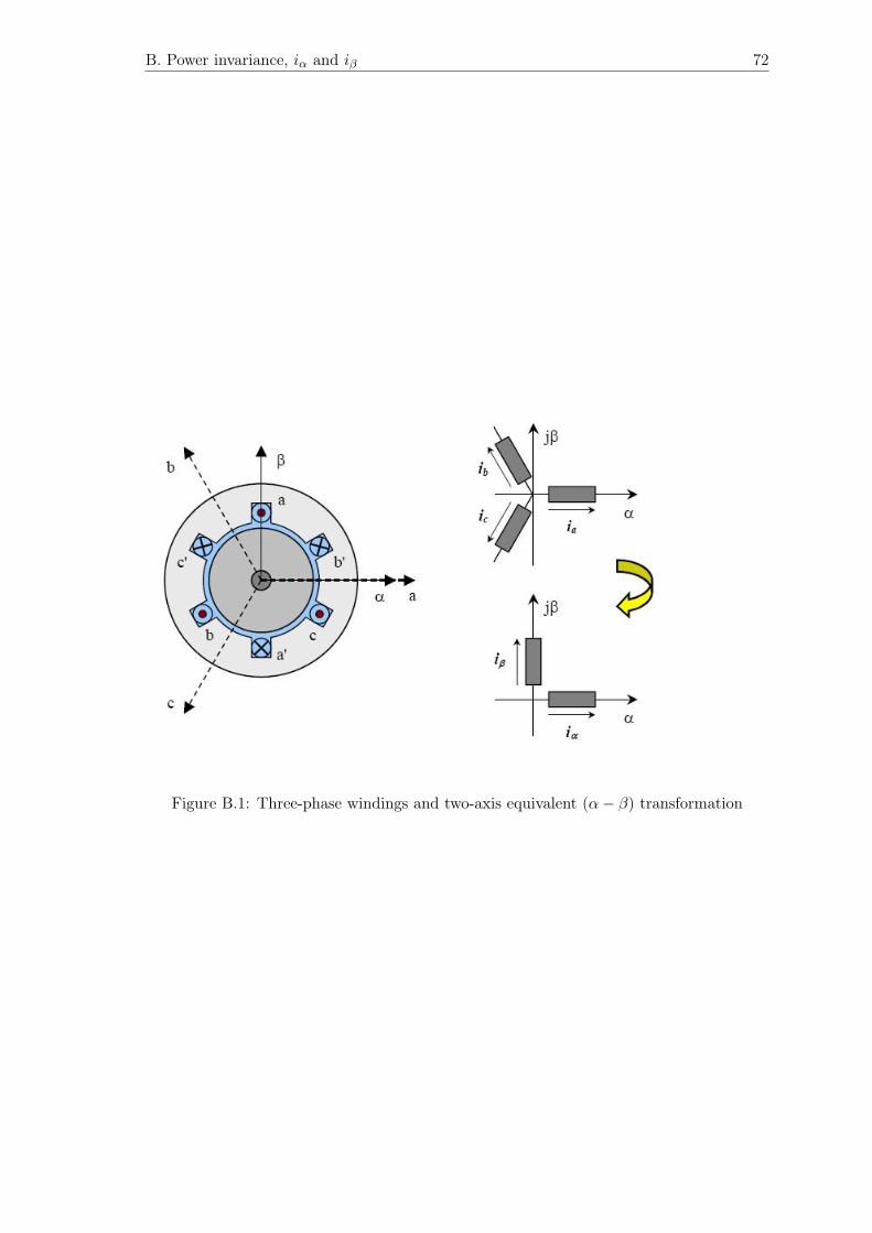
B. Power invariance, iα and iβ 72
Figure B.1: Three-phase windings and two-axis equivalent (α− β) transformation

Appendix C
Direct vector control
Out (2.18):
~uS(t) = RS . ~iS(t) +d ~ΦS
dt
follows:
d ~ΦS = [ ~uS(t)−RS . ~iS(t)].dt
⇒ ~ΦS =t∫0
[ ~uS(t)−RS . ~iS(t)].dt (C.1)
The rotor flux in stator-co-ordinates can be written as:
~ΦR.ejδ = L0.~iµ = L0.(~iS +LR
L0. ~iR.ejδ) =
L0
LS.
(LS . ~iS +
LR.LS
L0. ~iR.ejδ
)=
L0
LS.
(LS . ~iS +
L0.(1 + σR).L0.(1 + σS)L0
. ~iR.ejδ
)(C.2)
With: σ = 1− 1(1+σR).(1+σR) = 1− L0
2
LR.LS=total scatter coefficient of the inductionmotor
is: 11−σ = (1 + σR).(1 + σR)
So that:
~ΦR.ejδ =L0
LS
(LS . ~iS +
L0
1− σ~iR.ejδ
)=
L0
(1− σ)LS.[LS . ~iS(1− σ) + L0. ~iR.ejδ
]=
1(1− σ)(1 + σS)
[LS . ~iS + L0. ~iR.ejδ − σ.LS . ~iS
]= (1 + σR).[ ~ΦS − σ.LS . ~iS ]
~ΦR.ejδ = LRL0
.( ~ΦS − σ.LS . ~iS) = ΦR(α) + ΦR(β) (C.3)
If the motor parameters LR, LS , L0, σ and RS are known, than out of a measurement of~us and ~iS , the flux ~ΦR.ej.δ can be calculated with equations (C.1) and (C.3).The flux orientation is in principe possible without the use of a encoder or tacho. But theinfluence of the temperature on RS has to be compensated.
73
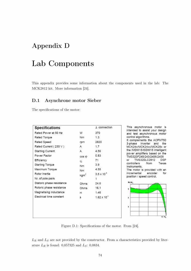
Appendix D
Lab Components
This appendix provides some information about the components used in the lab: TheMCK2812 kit. More information [24].
D.1 Asynchrone motor Sieber
The specifications of the motor:
Figure D.1: Specifications of the motor. From [24].
LR and LS are not provided by the constructor. From a characteristics provided by liter-ature LR is found: 0,057325 and LS : 0,0834.
74

D. Lab Components 75
D.2 Technosoft: ACPM750 - AC power module
Company info Technosoft
Tool Type Daughter Cards
Part Number 24TAN00111
Application(s) Industrial
DSP Generation (s) TMS320C24x Controllers , TMS320C28x Controllers
DSP device (s)
Form Factor Other
Related Product Info ACPM750 - AC power module
Price (USD) Contact company
Description: ACPM750 [24] is a three-phase IGBT power converter, usable with Tech-nosoft DSP modules based on TMS320C24x DSP controllers. Combined with one of thesemodules (MSK2407, MSK2812, MSK240, MSK243), an intelligent AC-drive unit in therange up to 750 W is obtained.
Features: 180-240 VAC line input, 50/60 Hz, 750 W power output, three-phase, 4 A,150% overload for 1 minute. Brake transistor. Isolated two currents and DC-link measure-ment. Integrated protections (short-circuit, earth / ground fault, over and under ? voltageand over-temperature). MC-bus compatible for connection with external DSP modules(as Technosoft MCK2407, MCK240, MCK243, IMMC24x, etc.). Ideal for evaluation, im-plementation and experimentation on DMC structures with full digital control structure.Usable with all Technosoft development and analysis software platforms, as DMCD-Pro,DMCS, Motion Studio.
D.3 Powersupply Diametral P230R51D
Description: Laboratory power supply P230R51D is determined for each professionaland amateur laboratory. Its characteristics can be evaluated especially by developmenttechnicians, repairmen of consumer electronics, manufacturers and last but not least alsoby the vocational schools.It is equipped by two power supplies with flowing voltage regulation in the range of 0 - 30Vwith possibility of setting a current limit from 0.1 - 4A. In addition, this model disposes ofa consistent voltage source 5V/3A. Adjustable part of source is provided with measuringdevices for voltage and for current as well. Indication of exceeding the current limit isperformed by flashing decimal point on the appropriate current measuring device and byintermittent sound signal. This sound signal can be switched off according to the need.Outputs of individual sources are operated by a separate switch knob with the indicator forthe simple handling. Thanks to it there is not necessary to switch-off the whole laboratorypower supply during the work.
D. Lab Components 76
Furthermore, it is supplied with a switch knob for connection of adjustable sources intoone symmetrical source. Against the temperature overload it is prevented by temperaturesensor and ventilator, which can cool down the coolers of output elements to an acceptablevalue, in a case it is needed.Transformer is dimensioned enough for permanent maximal power output supply to load-ing.
D.4 Function generator SFG-830
Description:
• 30MHz Direct Digitally Synthesized Source
• 20mHz Frequency Resolution
• +10ppm Frequency Accuracy
• 12Bit, 5M Sample/S Arbitrary Waveforms
• Sine, Triangle, Ramp and Square Waveforms
• Internally Synthesized FM, AM and Phase Modulation (PSK)
• Low distortion
• RS232 interface
• Arbitrary Modulation
• Linear and log sweeps
• Optional IEEE-488 Interface only for SFG-830G
• Free Arbitrary Waveform Composer Software for Windows 95/98/2000
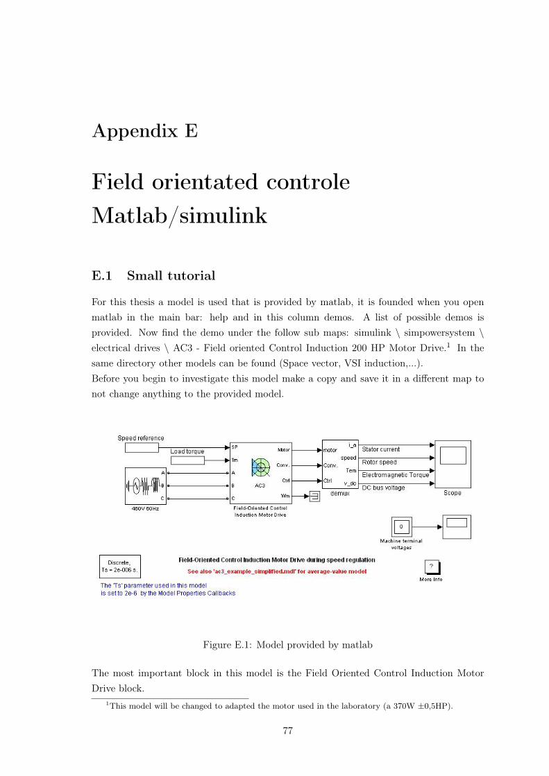
Appendix E
Field orientated controleMatlab/simulink
E.1 Small tutorial
For this thesis a model is used that is provided by matlab, it is founded when you openmatlab in the main bar: help and in this column demos. A list of possible demos isprovided. Now find the demo under the follow sub maps: simulink \ simpowersystem \electrical drives \ AC3 - Field oriented Control Induction 200 HP Motor Drive.1 In thesame directory other models can be found (Space vector, VSI induction,...).Before you begin to investigate this model make a copy and save it in a different map tonot change anything to the provided model.
Figure E.1: Model provided by matlab
The most important block in this model is the Field Oriented Control Induction MotorDrive block.
1This model will be changed to adapted the motor used in the laboratory (a 370W ±0,5HP).
77
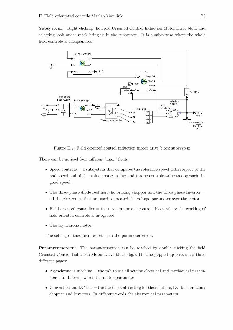
E. Field orientated controle Matlab/simulink 78
Subsystem: Right-clicking the Field Oriented Control Induction Motor Drive block andselecting look under mask bring us in the subsystem. It is a subsystem where the wholefield controle is encapsulated.
Figure E.2: Field oriented control induction motor drive block subsystem
There can be noticed four different ’main’ fields:
• Speed controle = a subsystem that compares the reference speed with respect to thereal speed and of this value creates a flux and torque controle value to approach thegood speed.
• The three-phase diode rectifier, the braking chopper and the three-phase Inverter =all the electronics that are used to created the voltage parameter over the motor.
• Field oriented controller = the most important controle block where the working offield oriented controle is integrated.
• The asynchrone motor.
The setting of these can be set in to the parameterscreen.
Parameterscreen: The parameterscreen can be reached by double clicking the fieldOriented Control Induction Motor Drive block (fig.E.1). The popped up screen has threedifferent pages:
• Asynchronous machine = the tab to set all setting electrical and mechanical param-eters. In different words the motor parameter.
• Converters and DC-bus = the tab to set all setting for the rectifiers, DC-bus, breakingchopper and Inverters. In different words the electronical parameters.
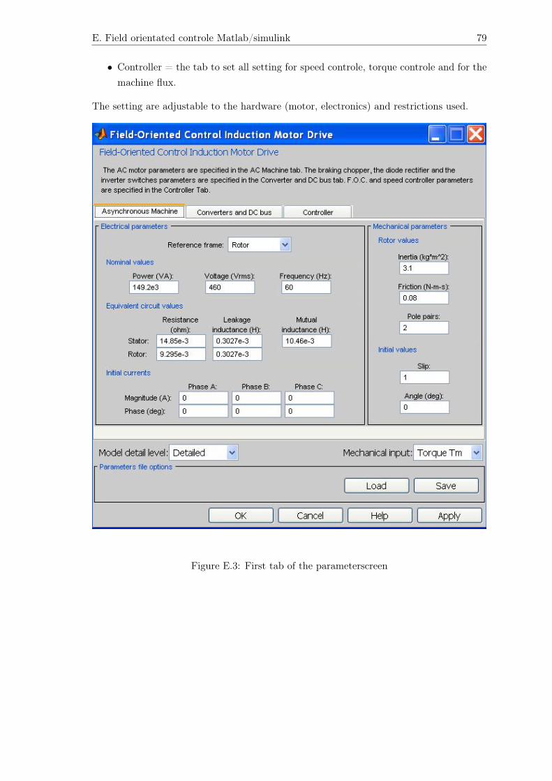
E. Field orientated controle Matlab/simulink 79
• Controller = the tab to set all setting for speed controle, torque controle and for themachine flux.
The setting are adjustable to the hardware (motor, electronics) and restrictions used.
Figure E.3: First tab of the parameterscreen