1

University of Malta Engines

Introduction:

Engine simulation has become an integral part of engine development. Although it cannot be used

independently from physical experimentation, it can still potentially reduce experimentation time in

the sense that the main regions of physical experimentation can be chosen from the full spectrum of

experiments.

The three authors presenting this work have modest experience in the field of internal combustion,

particularly in the areas of engine simulation, electronic fuel injection implementation, mechanical

engine friction and valvetrain design. In this assignment, these areas were combined to provide a

holistic approach. It is to be brought to attention that none of the contributors had previous

experience with GT-Suite or ModeFRONTIER. In previous work, engine simulation was usually

carried out with Ricardo WAVE, which was introduced in MEC4011 Power Plants module [1].

This challenged the team to familiarise ourselves with GT-Suite, and convert our previous

knowledge on engine simulation to provide the required deliverables, along with some experimental

tests carried out at the Thermodynamics Lab of University of Malta. Apart from the preparatory

work in previous months the team devoted around 250 hours collectively in the last week before

submission.

Air Filter Flow Testing:

Prior to modelling the complete intake system, it was thought to be of an educational value to flow

test several air filters and compare their performance. In total, four air filters were flow tested using

a centrifugal blower, where the air filter was connected to the suction side of the blower through a

50mm diameter smooth pipe. A properly sized hole along the diameter of the pipe was drilled

500mm (10D) downstream of the air filter and smoothened to suit a pitot static tube traversing the

flow. The difference in pressure between the dynamic and static ports of the pitot tube was read

from an inclined manometer, from which the peak fluid velocity was found. The blower’s rotational

speed was varied by a variable frequency drive and the range between 10Hz to 60Hz was covered,

which in total resulted in a spectrum between 9.6g/s and 80g/s.

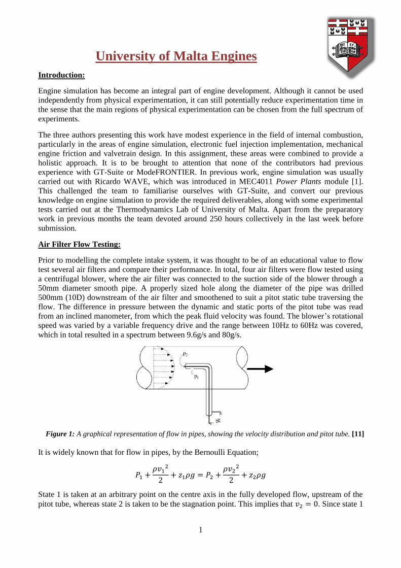
It is widely known that for flow in pipes, by the Bernoulli Equation;

𝑃1 +𝜌𝑣1

2

2+ 𝑧1𝜌𝑔 = 𝑃2 +

𝜌𝑣22

2+ 𝑧2𝜌𝑔

State 1 is taken at an arbitrary point on the centre axis in the fully developed flow, upstream of the

pitot tube, whereas state 2 is taken to be the stagnation point. This implies that 𝑣2 = 0. Since state 1

Figure 1: A graphical representation of flow in pipes, showing the velocity distribution and pitot tube. [11]

2

and state 2 are on the same elevation, the two potential energy terms cancel out from both sides of

the equation, which results in:

𝑃1 +𝜌𝑣1

2

2= 𝑃2

=> 𝑣1 = √2(𝑃2 − 𝑃1)

𝜌 … (1)

By the 1/7th

power law, the average velocity 𝑣𝑎𝑣𝑔 is equal to 0.82 of the peak velocity. [2]

∴ 𝑣𝑎𝑣𝑔 = 0.82𝑣1

Therefore, the volumetric flow rate may be found as:

𝑄 [𝑚3/𝑠] = 𝐴𝑝𝑖𝑝𝑒𝑣𝑎𝑣𝑔 … (2)

The graph of the volumetric flow rate against the change in pressure across the air filter was plotted

in Figure 2 for all the air filters tested.

As can be seen from Figure 2, the larger filters, being the Mahle, Tecneco and K&N twin barrel

filters showed better flow characteristics than the small K&N SU HS4 and the KK150 filters. Table

1 shows the respective flow areas of each air filter and according to such values, the flow curve of

each filter were corrected for a common flow area. The resulting graph is shown in Figure 3.

0

0.01

0.02

0.03

0.04

0.05

0.06

0.07

0.08

0.09

0 500 1000 1500 2000 2500 3000 3500 4000

Q [

m3

/s]

∆P [Pa]

Mahle LX646/1

Tecneco AR216

K&N SU HS4 (Used, Pre-Clean)

PiperCross KK150 (Used)

K&N SU HS4 (Used, Post-Clean with K&N Oil)

K&N Twin Barrel (Used, Post-Clean)

K&N Twin Barrel (Used, Post-Clean with K&N Oil)

1

3 4

2 5

7

6

Table 1: The respective flow areas of each air filter.

Air Filter Effective Flow

Area [cm2]

Normalised

Areas [cm2]

Mahle LX646/1 362.56 7.71

Tecneco AR216 673.20 14.31

K&N SU HS4 47.04 1.00

PiperCross KK150 20.15 0.43

K&N Twin Barrel 231.04 0.49

Figure 2: The graph of Volumetric Flow Rate [m3/s] against DeltaP [Pa]

3

The trendline equations and R-squared values for the filters plotted in Figure 3 are given in Table 1.

Table 2: The trendline equations for the respective air filters of Figure 3. Curve No. Trendline Equation R-Squared Value

1 𝑄𝑐 = −(1𝑥10−8)∆𝑃2 + (8𝑥10−5)∆𝑃 0.9663

2 𝑄𝑐 = −(5𝑥10−9)∆𝑃2 + (3𝑥10−5)∆𝑃 0.8608

3 𝑄𝑐 = −(4𝑥10−9)∆𝑃2 + (3𝑥10−5)∆𝑃 0.9400

4 𝑄𝑐 = −(2𝑥10−9)∆𝑃2 + (1𝑥10−5)∆𝑃 0.9608

5 𝑄𝑐 = −(2𝑥10−9)∆𝑃2 + (1𝑥10−5)∆𝑃 0.9458

6 𝑄𝑐 = −(3𝑥10−9)∆𝑃2 + (1𝑥10−5)∆𝑃 0.9462

7 𝑄𝑐 = −(1𝑥10−9)∆𝑃2 + (5𝑥10−5)∆𝑃 0.9674

Normalising the flow curves to a common effective flow area, allows an easy comparison of the

filtration material. Evidently, Figure 3 shows that the PiperCross filter has superior flow

characteristics (to the detriment of filtration due to large pores) compared to the other filters.

Figure 4: The air filterflow test setup

0

0.02

0.04

0.06

0.08

0.1

0.12

0.14

0 500 1000 1500 2000 2500 3000 3500 4000

Q_C

om

pe

nsa

ted

[m

3/s

]

∆P [Pa]

Mahle LX646/1

Tecneco AR216

K&N SU HS4 (Used, Pre-Clean)

PiperCross KK150 (Used)

K&N SU HS4 (Used, Post-Clean with K&N Oil)

K&N Twin Barrel (Used, Post-Clean)

K&N Twin Barrel (Used, Post-Clean with K&N Oil)

1

2 3

4 5

7 6

Figure 3: The graph of compensated volumetric flow rate [m3/s] against DeltaP [Pa].

4

The two K&N filters (SU HS4 and Twin Barrel), believed to have the same filtration material

seemed to have significantly different flow characteristics, which may be originating from the shape

of the respective filters. The K&N SU HS4 filter performed better before the cleaning treatment. It

is in the opinion of the authors that the application of the treatment oil to the filter according to the

manufacturer specification has impeded slightly the flow characteristics, which however is deemed

to improve the filtration characteristics.

Constructing the Single Cylinder 250cc Model in GTI-ISE 7.5:

To familiarise ourselves with GT-Suite, the “Engine Performance Tutorial” was read and the

relevant models were built successfully. As a start point for this work, the “1cylSI-final.gtm”

example model was used. To suit the aim of this assignment, several modifications had to be done

to the example, the first one being to convert the engine to a 4-valve configuration.

The base intake and exhaust valve lift profiles were obtained from the GT-ISE 7.5 ‘template.gtm’. It

was noted that such valve lift curves had a very small duration with negligible overlap.

Increasing the engine speed reduces the amount of time available for the fresh intake charge to be

induced in the cylinder and the exhaust gases to be expelled. To improve considerably the

volumetric efficiency of the engine at higher engine speeds, the duration for both valves should be

adequately increased.

Increasing the intake valve duration would mean that the valve opens at the end of the exhaust

stroke and closes during compression. It is usually desirable to account for the width of the lift

curve due to a larger duration by shifting the curve to the exhaust stroke, meaning that the intake

valve starts opening at around 52𝐷𝑒𝑔 𝐵𝑇𝐷𝐶. Apart from increasing the time in which the intake

charge can be induced, volumetric efficiency also benefits from the effect of the displacement phase

of the exhaust stroke.

Similar reasoning was applied to the exhaust valve. If the exhaust valve opens at around

72𝐷𝑒𝑔 𝐵𝐵𝐷𝐶, the incylinder pressure which would still be at a reasonably high value would create

a large differential pressure across the exhaust valve and consequently improves to a great extent

the scavenging effect through an improved blowdown phase.

To apply this reasoning to our model, the graphs acquired from the ‘template.gtm’ were modified

extensively. The intake lift curve was made to have an initial estimate of 210 Deg duration at 1mm

lift, with an anchor at 230Deg from TDC firing. The exhaust valves were made to have an initial

duration of 210 Deg at 1mm lift and an anchor at 130 Deg from TDC firing. This meant that the

initial valves overlap was of 112 Deg. All the angles given are in crank angle. Both the lift and

duration of both the intake and exhaust valves were parameterised with variable names [intdur],

[intlift] for the intake valve and [exhdur], [exhlift] for the exhaust valve respectively through a

multiplier. Unfortunately, since the number of parameterised variables was quite large, the anchor

had to be fixed and thus wasn’t optimised. Even though having faced this limitation, the overlap of

the intake and exhaust valves was still varied through the variation of the valve durations.

Initially the flow coefficients for the intake and exhaust valves were both imported from the

‘template.gtm’ however after running the simulation once, it was noticed that an error was shown

which said that due to a large ratio of 𝐿/𝐷, the computation outrun the curve range. This meant that

either the maximum 𝐿/𝐷 had to be reduced by reducing the maximum lift or increasing the valve

diameter or otherwise another flow coefficient curve had to be used. The team opted for the second

option, and the flow coefficients used were those reported by Farrugia [3], as obtained on a flow

bench test of a Honda F2 600cc engine. When such flow coefficient graphs were compared with

5

that of the ‘template.gtm’, both graphs showed similar values, however that acquired by Farrugia

[3] had a slightly larger range which allowed the necessary computations.

Constructing the Elements:

After converting the “1cylSI-final.gtm” example to four valves, the two intake valves were

connected with a Y-Junction through a small length of pipe. This was also applied for the exhaust

side. The two Y-Junctions were in turn connected to a small length of pipe to model the remaining

portion of the intake and exhaust ports. Figure 5 shows the elements incorporated.

On the intake side of the engine, a bellmouth was assigned with a small length of round pipe to

introduce the air into the throttle body. The bellmouth was also used as the mass flow sensor

element to compute the mass of fuel injected in retaining the AFR constant. It was noted that the

default value of 6g/s for the mass flow rate of the injector had to be increased to 10g/s. For the

default value of 6g/s, the engine speed ranges higher than 14000RPM were noticed to have an AFR

of around 17:1.

The throttle body diameter was parametrised by the variable [D_Throttle]. Downstream of the

throttle body, the intake runner was modelled with a round pipe. Both the diameter and the length of

the runner were parameterised with variable names [intrunnerdiameter] and [intrunnerlength]. The

small piece of round pipe between the bellmouth and the throttle body was fixed with a diameter of

52mm and a length of 60mm. Since the engine was to be operated up to speeds of 17500RPM, the

intake lengths were initially kept short with a generous diameter. The length of the round pipe

between the bellmouth and the throttle was however not parametrised due to limit on computational

power.

With regards to Thermal and Pressure Drop considerations on the intake system, the wall

temperatures of the bellmouth connection and the intake runner were both assigned as 300K due to

Figure 5: The model including the ports, runners, valves and throttle.

6

the fact that they are in constant contact with cool intake air. The surface roughness of both the

bellmouth connection and the intake runner were considered to be similar to smooth plastic.

The intake port elements were all deemed to be frictionless (as stated by Farrugia [3] due to the fact

that the flow bench tests Cd also incorporates the wall friction) with wall temperatures of 373K.

This particular temperature was chosen to symbolise the cylinder head temperature, with which the

intake air comes in contact in the intake port. The two pipes closest to the intake valves were both

parametrised on the length with variable [intvalveportlength]. The diameter of these two pipes was

made equal to the valve diameter which was parameterised with a variable name [D_ASP]. The

single round pipe connecting to the intake Y-junction was also parameterised on its length and

diameter with variable names [intportlength] and [intportdiameter] respectevely. The flow split

general element was assigned with a constant volume of 31808𝑚𝑚3and a default constant surface

area.

For the first initial runs, the airbox volume was not modelled. However after familiarising ourselves

with the software and the aircleaner flow tests were conducted, the model was modified to include

the airbox. Furthermore a Co-Simulation using GT-Suite and Fluent was also done and explained in

detail later in the text.

The exhaust side of the engine was modelled with two simple lengths of round pipe; one of which

modelled the exhaust runner, and one modelled a small piece of exhaust pipe. The pipe modelling

the exhaust runner was parametrised on the length and diameter with variable names [exhrunlength]

and [exhrundiameter] whereas the small piece of exhaust pipe was modelled with a fixed length of

200mm and a diameter equal to that of the exhaust runner.

The exhaust duct in head was modelled as a Y-Junction connected through two small lengths of

round pipe to the valve. Downstream of the Y-Junction, a round pipe element was assigned which

model the remaining length of the exhaust port. The length and diameters of the two similar pipes

were assigned with the same parametrised diameter, having a variable name of [D_SCA]. The same

pipes were also optimised on their length with variable name [exhvalveportlength]. The other pipe

connected to the Y-Junction was parametrised on both the length and diameter with variable names

of [exhportlength] and [exhportdiameter] respectively.

The thermal aspect of the exhaust duct in head was modelled with a temperature of 373K which

represents the cylinder head temperature, with which the exhaust comes in contact. The roughness

of the same port was assigned to be frictionless.

The intake runner was assigned with a roughness similar to that of cast iron with a wall temperature

computed from the ‘WallTempSolver’ sub model, factoring cylindrical geometry, material

properties, external temperature, radiation and convection. The external convection coefficient was

taken to be 15𝑊/𝑚2𝐾. The external convection temperature and radiation sink were both

considered to be 323K which represents the exhaust environment temperature.

Compression Ratio:

The compression ratio used in this model was fixed to 12:1, which is a reasonable value for a

motorcycle engine. The possibility of increasing the compression ratio to the maximum allowed by

the specifications was discussed, however it was agreed that going beyond the 12:1 limit would

create a problem with the fuel chosen. For this model the standard GT Suite Fuel (Indolene) was

used which has a RON rating of 98 [4], whereas commercially available fuel usually has a RON

rating of 95.

7

For the compression ratio to be optimised it would be ideal to include a knock model in the

simulation and the compression ratio can be increased to a suitable safe limit which prohibit

autoignition.

From experiments done by Azzopardi [5] on a 600cc Kawasaki ZX6r engine, the knock magnitude

was investigated from incylinder pressure measurements and compared to feedbacks from

commercial knock sensors. The frequencies of knock were also investigated through computations

of the Fast Fourier Transform. Due to the AVL ZL21 sideways oriented pressure sensing

diaphragm, only the first mode of knock could be captured. Another section of this study regarded

the calibration of the commercially available knock sensor with the data acquired from the

incylinder pressure measurments. The commercially available sensor was then connected to the

ZX6r programmable Reata engine management.

From previous work by Grech [6] on 1D engine simulation it was noticed that knock models are not

reliable in capturing knock, and furthermore require intense computational power. Thus for the

scope of this assignment the compression ratio could not be decided based on knock study and

hence a conservative value of 12:1 was implemented.

Design of Experiment:

One of the fundamental learning experiences of this work regarded the Design of Experiments

(DOE) and the respective optimisations. After the complete model was built, the parametrised

geometries described in the previous section were to be optimised.

In total nineteen parametrised variables were assigned. This made it computationally impossible to

run the experiments in one batch, thus these were split up over two batches with the intake

experiments and optimisations done separately and independently of the exhaust side. According to

Sammut [7], the optimisations on the intake can be run separately from the exhaust. This was also

confirmed from a simple model which the authors ran on the same single cylinder engine with the

intake and exhaust optimisations run at once but for a very small engine speed range and limited

number of parameters. The interactions obtained from this run are plot in Figure 6.

As can be seen from the above figure, the interaction effect of intake runner and the exhaust runner

as obtained from the variables [intrun] and [exhrun] are minimal.

Figure 6: The interactions of the intake and exhaust showing negligible effect on the torque and

power.

8

The Design of Experiment type was chosen to be the Full Factorial. This type assigns all number of

permutations required by the number of variables assigned as experiment parameters. The range of

variation of each parameter was determined by assigning the minimum and maximum values, and

each range should then be split into the desired number of levels. The number of levels determines

the number of experiments that would be carried out in the Full Factorial type of DOE.

After splitting up the intake and exhaust DOE’s it was still noticed that the total number of

experiments exceeded the ten thousand which requires distributed simulation. Thus to keep the

number of experiments below the ten thousand mark the number of levels was set was quite a rough

value which unfortunately reduced the resolution of the model. Two different strategies to

overcome this limitation were thought of. The first is to run the detailed fine levelled experiments

on a very short Engine Speed range with just two levels of engine speed. This would then maximise

the torque by optimising all the parametrised variables for the two levels of engine speed. By doing

the same procedure for the global range of engine speed in steps of two would then result in a set of

optimised parameters for each level of engine speed. This would attain a high resolution of the

variables to be parametrised without exhausting the available computational resources.

The other simpler strategy which was used for this assignment due to time restrictions was to run a

model with different cases to obtain a general torque curve with engine speed. From this graph, the

salient points which represent the region of operation of the engine was chosen and the DOE was

then run only on this region of interest of engine speed with only five levels. Such method

decreased the number of experiments to an acceptable level, however limited both the range and

resolution of the model. Figure 7 shown below shows the general non-optimised torque curve.

As can be seen, a torque dip is seen at the range of engine speeds between 7000RPM and

9000RPM, whereas a peak torque of 25Nm was seen at 11000RPM. Beyond this region, the torque

falls to around 15Nm. Since the engine was designed to rev up to 17500RPM, speeds below the

5000RPM mark were seen to be superfluous for the particular engine. Thus the range of

optimisation was chosen to be between 5000RPM and 17500RPM. The five levels of optimisation

were stratified by the 5000RPM, 8125RPM, 11250RPM, 14375RPM and 17500RPM.

In order to assess power curves with good judgement the drop in engine speed for each gear shift

from 17,000rpm was found. Gear ratios for a racing motorcycle, namely a Honda CBR250RR were

found. The ratios were as follows: 2.733, 2.000, 1.590, 1.333, 1.153, 1.035 and typical ratios for

primary reduction, final reduction and wheel size were used. This resulted in a calculated from

17000 to approximately 12000 rpm between 1st and 2

nd gear. It is noted that this drop is the biggest

0

10

20

30

40

50

0

20

40

60

80

100

120

0 2000 4000 6000 8000 10000 12000 14000 16000 18000 20000

Torq

ue

[N

m],

Bra

ke P

ow

er

[Hp

]

Vo

lum

etr

ic E

ffic

ien

cy [

%]

Engine Speed [RPM]

Volumetric Efficiency [%]Torque [Nm]Brake Power [Hp]

Figure 7: The graph of volumetric efficiency, brake power and torque with engine speed.

9

drop as the drops in other up shifts result in progressively smaller drops in RPM. The range of

engine speeds found was covered by the five levels of optimisation.

The first run of experiments was for the intake side of the engine. Table 3 below shows the range of

variation for each variable and the number of levels. The total number of experiments done was

2560. The R-square value for the curve fitting was found to be 0.68.

Table 3: The parametrised variables, their ranges and levels for the intake side {DOE_intake_no1}

Parametrized Variable Minimum Maximum No. of Levels

Engine Speed 5000 17500 5

D_ASP 33 35 2

D_Throttle 49 52 2

intDur 1 1.2 2

intLift 1 1.1 2

Intportdiameter 38 41 2

Intportlength 13 17 2

Intrunnerdiameter 49 52 2

intrunnerlength 60 80 2

intvalveportlength 12 14 2

No. of Experiments 2560

The Second run of experiments regarded that of the exhaust. The parametrised variables together

with their ranges and number of levels are shown in Table 4. The number of experiments performed

was 9720. Since the number of experiments by the Full Factorial reached high values, the

compilation of experiments took three hours and twenty minutes to complete. Due to the memory

limitation the curve fitting of the experiments had to be split into two by the engine speed

categories. The R-squared values of the two fits were 0.94 and 0.9992. This is explained in detail

further on. Table 4: The parametrised variables, their ranges and levels for the exhaust side

{DOE_exhaust_no1}

Parametrized Variable Minimum Maximum No. of Levels

Engine Speed 5000 17500 5

D_SCA 26 27 2

Exhdur 1 1.2 3

Exhmult 0.9 1.1 2

Exhportdiameter 43 46 3

Exhportlength 20 30 3

Exhrundiameter 44 46 2

exhrunlength 180 220 3

exhvalveportlength 22 27 3

No. of Experiments 9720

Optimisation:

After having run the design of experiments in GT-ISE, the torque was maximised for each engine

speed and the optimum parameters for obtaining the best torque at each engine speed were

consequently found. Different engine speed ranges require different optimum parameters. This

imposes a physical limitation on engine design, for example to vary the duration of valves, variable

valve timing would be required, similarly intake runner lengths can also be varied to cater for

different engine speeds. The optimum parameters at each engine speed are given in Table 5 and

Table 6.

10

Table 5: The optimum parameters for {DOE_intake_no1} at each engine speed [RPM] RPM INTDUR INTLIFT INTPORTDIA INTPORTLENGTH INTRUNDIA INTRUNLENGTH

5000.0 1.0 1.0 38.1 13.0 49.2 76.8

8125.0 1.0 1.1 38.0 13.0 49.6 79.4

11250.0 1.0 1.1 38.0 13.0 51.0 79.4

14375.0 1.2 1.1 38.0 15.0 49.0 80.0

17500.0 1.2 1.1 38.0 13.0 49.0 80.0

Table 6: The optimum parameters for {DOE_intake_no1} at each engine speed [RPM]

RPM D_ASP D_THROTT RPM INTVALVEPORTLENGTH TORQUE BHP

5000.0 33.1 50.9 5000.0 12.0 22.9 15.2

8125.0 35.0 49.1 8125.0 12.0 24.8 30.0

11250.0 34.7 52.0 11250.0 13.7 24.8 36.1

14375.0 35.0 49.4 14375.0 13.0 21.6 43.2

17500.0 35.0 52.0 17500.0 13.0 17.1 41.6

To simplify matters, a compromise was reached between the optimum values of each engine speed.

These carefully-chosen parameters were then assigned as constants to the model and the latter was

run with cases of engine speed at 500RPM intervals. The torque curve with the optimum parameters

from the DOE and the torque curve with carefully-chosen parameters were plot as curve 1 and

curve 3 respectively in Figure 8. As can be seen from the graph, curve 1 which is supposed to have

optimum torque for each engine speed seemed to be considerably different as compared to curve 3.

It is observed that the curve which was supposed to give the optimum torque at all engine speeds,

ie. curve 1, developed 4bhp less than the curve 3, which if anything is expected to be less than

optimum due to the compromises required in the selection process. This observation was not well

understood.

In curve 3 which shows the plot for the carefully-chosen parameters it was noticed that there was a

flat portion between the 6000RPM and the 8000RPM. Furthermore, the torque beyond the

9500RPM seemed to drop abruptly. To try and improve in general the power curve, the duration of

the intake valve was increased by a factor of 1.1 and 1.2 consecutively, with the curves being 4 and

5 respectively. It was however noticed that increasing the intake duration worsened the torque

distribution over the speed range between 6000RPM and 9000RPM.

0

10

20

30

40

50

2000 4000 6000 8000 10000 12000 14000 16000

Bra

ke P

ow

er [

bh

p]

Engine Speed [RPM]

1 3 4 5

Figure 8: The graph of power against engine speed for the optimised intake system

{DOE_intake_no1}.

11

Retaining the intake duration with the 1.2 factor, the intake runner length was varied by 30mm from

a minimum of 60mm to a maximum of 90mm. In Figure 9, the plot corresponding to the run with

60mm intake runner length is plot 6 and the one corresponding to 90mm runner length is plot 7. To

aid high engine speed regions, it is usually advisable to reduce the length of the port and increase

the diameter, however from such plots when the intake runner length was decreased from 90mm to

60mm, a noticeable decrease in power was observed from around 6000RPM all the way to the

17500RPM. Since the curve of the 90mm runner length seemed to develop slightly higher power,

the intake runner length was chosen to be 80mm to strike a balance between the two extremities

while still giving priority to the longest runner. Curve 7 shows a pronounced dip at the 7500RPM.

To try and improve this dip together with reducing the negative gradient at the 17000RPM, the

exhaust runner was shortened from the constant value of 400mm as run in the DOE experiment to

300mm. The torque curve of the 80mm intake runner length together with the 300mm exhaust

runner are shown in curve 8. As can be seen from the plot, curve 8 shows a significant improvement

over the previous case 7. The dip at around the 8000RPM was straightened, whilst the negative

gradient at the 7000RPM range was decreased to a great extent. To try and improve slightly more

on this condition, the 300mm exhaust runner was reduced to just 200mm and the power curve for

this case was plot in curve 9. This plot showed a slight improvement at the 8500RPM region,

however it also showed a significant decline in power at the 11000RPM.

After optimizing the intake side of the engine, the same procedure was implemented on to the

exhaust side. The DOE model was run and the optimum values were chosen for each engine speed

range. It must be noted that for such DOE, the number of experiments by the Full Factorial reached

the 9700 mark. This large number of experiments created some issues with the fitting of the model

surface. The reason was that GT-Power was only using a small portion of the computer’s RAM

(irrespective of using a 4Gb,8Gb or 32Gb RAM computer), and thus it was reported that

insufficient memory was detected. To overcome this limitation, the engine speed range was split

into two overlapping sections for the post-processing of the DOE experiment. As can be seen in

Figure 10, plots 1 and 2 seem to overlap at the 11500RPM with a shift of 1.15BHP. It was also

observed that there was a slight change in gradient at the overlap.

The optimum parameters found for the intake were not inserted in the DOE for the exhaust side, for

the simple reason that both DOE’s were run at the same time. However the data for the intake side

was processed before that of the exhaust side, and thus for the exhaust side, after the carefully-

chosen values were chosen from the DOE optimum values, the model was rerun with cases at every

0

5

10

15

20

25

30

35

40

45

50

2000 4000 6000 8000 10000 12000 14000 16000

Bra

ke P

ow

er

[bh

p]

Engine Speed [RPM]

6

7

8

9

Figure 9: The graph of power against engine speed for the optimised intake system

{DOE_intake_no1} - Continued.

12

500RPM interval. For such run, the optimum values obtained from the intake model were input to

the exhaust cases. This in fact shows in the improvement beyond the 12000RPM range and at the

8000RPM region.

A point which should be mentioned is that the DOE for the intake system described previously was

run on a model on which the airbox was not modelled. To capture the effect of the air box whilst

monitoring its effect on the already optimised intake parameters, another DOE was run for the

intake side, with the airbox modelled as a flow split general. The parametrised variables in this

DOE were listed in Table 7 with a total of 7680 experiments. Since the experiment number was also

large, the surface fitting had to be split into two, with R-squared values of 0.67 and 0.997.

Table 7: The parametrised variables, their ranges and levels for the exhaust side

{DOE_intake_no2}

Parametrized Variable Minimum Maximum No. of Levels

Engine Speed 5000 17500 5

D_ASP 33 35 2

D_Throttle 49 52 2

Intdur 1 1.2 3

Intlift 1 1.1 2

intportdiameter 38 41 2

Intportlength 13 17 2

Intrunnerdiameter 49 52 2

intrunnerlength 60 80 2

Intvalveportlength 12 14 2

aboxvolume 0.5e6 1.2e6 2

No. of Experiments 7680

After running the DOE experiment, the best power curves were each plot as obtained from the

optimum parameters at each engine speed. This is seen in curves 1A and 1B in Figure 11. Similarly

to what was done for the previous DOE’s, from the DOE optimum values, a set of carefully-chosen

values were found and imposed as constants on the model and the latter was run with several cases

on engine speed. Curve 2 shows the graph for these carefully-chosen values. The variation between

curves 1A and 1B as compared to curve 2 occurs from the fact that for curve 2, the optimum

exhaust parameters as found from the previous DOE were input.

0

10

20

30

40

50

60

0 2000 4000 6000 8000 10000 12000 14000 16000 18000

Bra

ke P

ow

er

[BH

P]

Engine Speed [RPM]

1

2

3

Figure 10: The graph of Brake Power against Engine Speed for the design of experiment

{DOE_exhaust_no1}

13

To investigate the effect of the airbox volume, the optimum value found of 1.2Litres was varied to

both 0.5L and 2.2L. The curves for the 2.2L, 0.5L and 1.2L airbox are shown in Figure 11 and

Figure 12 as plot 4, 5 and 6 respectively.

To understand the concept of the expansion diameter, the model was run with an airbox volume of

1.2L, but with a reduced expansion diameter from 170mm to 100mm. The resulting curve is seen in

plot 6, which is very similar to plot 5, the one for the 1.2L volume and 170mm expansion diameter.

Another run was done with to compare the exact same model with no airbox. The resulting curve

was plot in 9. As can be seen, the airbox was responsible for a pronounced drop in power over the

entire range between 8500RPM and 14500RPM.

To smoothen the crests and troughs seen between the 7000RPM and the 12000RPM on curves 5

and 6, the exhaust runner lengths were reduced from the optimum values previously found in

{DOE_exhaust_no1} of 300mm to 150mm. The resulting curve was plot in 7. This showed a

significant improvement in averaging the crests and troughs found at the discussed regions. Another

0

5

10

15

20

25

30

35

40

45

50

0 2000 4000 6000 8000 10000 12000 14000 16000 18000 20000

Po

we

r [B

HP

]

Engine Speed [RPM]

1A

1B

2

3

0

5

10

15

20

25

30

35

40

45

50

0 2000 4000 6000 8000 10000 12000 14000 16000 18000 20000

Bra

ke P

ow

er

[BH

P]

Engine Speed [RPM]

4 5

6 7

8 9

Figure 11: The graph of Brake Power against Engine Speed for the design of experiment

{DOE_intake_no2}

Figure 12: The graph of Brake Power against Engine Speed for the design of experiment

{DOE_intake_no2} - Continued

14

run with the exhaust runner equal to 100mm was conducted, however as seen by comparison

between curves 7 and 8, no significant difference was seen.

Friction Coefficient Estimation:

Engine friction is one of the variables responsible in reducing engine performance. Friction

manifests itself on a significant scale in certain areas of engine operation. It is reported by Singh [8]

that engine friction consumes as much as 10% of the power output of the engine at full load, to

100% of the power output at no load. The Stribeck diagram is one of the tools that can be used to

identify the nature of the friction, depending on the operating regime of the particular component.

The Stribeck diagram plots the coefficient of friction against a dimensionless parameter being a

function of mean velocity and load.

The two extremes of operation are boundary friction and hydrodynamic friction. Boundary friction

refers to a direct metal-to-metal contact between two respective components. On the other hand

hydrodynamic lubrication refers to the instant when two surfaces are completely isolated by a layer

of circulating oil. Reducing the engine load and increasing engine speed shifts the operation to

hydrodynamic.

To validate the friction estimated from the one dimension engine model, a friction model reported

by Singh [8] was applied on the major engine components to find their individual FMEP. The total

mean effective pressures were then summated to give the total FMEP as a variable with engine

speed. The resulting relationship of TFMEP with engine speed was then compared with that

obtained from the engine simulation. Both traces were superimposed on Figure 13.

The one dimensional model was based on the Chen-Flynn correlation where the latter is described

by four terms to capture the effect of friction as dependent on several factors of operation. The

constant term captures the effect of accessory friction. The second term which varies linearly with

piston velocity captures the effect of hydrodynamic friction. Another term takes into consideration

the gas loading as represented by the peak combustion pressure. The last term varies in quadratic

manner and captures the effect of windage losses in the engine as a function of piston velocity [9].

The empirical friction correlations used were obtained by Singh [8]. It was argued that correlations

obtained by authors in the past were obtained from large industrial engines and such correlations

were thus inaccurate to predict friction on small scale engines. His interest was in particular in small

air cooled SI engines. Considering that the engine under consideration in this assignment is similar

to that considered by Singh [8], the empirical correlations reported in his work were used.

When considering friction, it should be explicitly stated which portion of friction is being

considered. Rubbing friction is the area of concern in this particular writeup. Rubbing friction refers

to the components of friction originating due to contact between two relative moving surfaces and it

can be further categorised by the main engine components. The main components under

consideration are:

1. Crankshaft Friction

2. Accessory Friction

3. Valvetrain Friction

4. Piston Assembly Friction

Crankshaft friction in particular originates from the interaction of the crank bearings with their

respective sleeve bearing. Bearings normally operate in the hydrodynamic region. This induces a

form of friction known as ‘turbulent dissipation’ which consists of energy lost in the process of the

15

pressurisation of the lubricant through the bearing orifices. The relationship used by Singh to

calculate crankshaft friction is:

The next category of rubbing friction is Accessory Friction. Such component is usually regarded as

varying in a linear proportion with engine speed, or otherwise it may also be taken as a constant.

Accessory friction refers to the power dissipated in ancillary components required in the operation

of an engine, such as; oil pump, water pump, alternator, fan drive and much more. Such forces are

reported to account up to 20% of the TFMEP according to Singh [8].

Valvetrain friction is another major source of friction. Several valvetrain configurations have their

associated friction distribution. It was reported by Heywood [10] that the overhead camshaft

configuration is the most efficient in terms of friction. The valvetrain system has two major friction

components; the spring force which increases the normal reaction, and the inertial forces. The

friction contribution coming from the spring force is significant at low engine speeds, whereas

inertial friction contribution is significant at higher engine speeds. The empirical relationship used

by Singh is given in the below equation.

Reciprocating friction refers to the component of rubbing friction which originates mainly from the

piston motion. The reciprocating piston has a complex transition between the hydrodynamic friction

and the boundary friction. Piston assemblies are usually modelled through four main forces; the gas

loading, the force transmitted through the connecting rod, the side thrust loading and the bore

frictional force. Near the bottom and top dead centres, since the velocity of the piston slows down

to a minimum the friction exhibited is of the boundary type, especially in the vicinity of TDC firing,

where apart from the low velocities experienced, the gas loading and high temperatures limit the

flow of lubrication between the contacting surfaces and thus boundary friction is promoted.

An Excel file with all the variables in the above equations was done and each of the friction

components was computed. The TFMEP graph obtained from Singh’s [8] work was then compared

to the curve obtained from GT-Power, as computed by Chen-Flynn’s correlation. The two graphs

can be seen in Figure 13. It should be noted that when Singh’s correlation with all its components

was used, a very high FMEP resulted. For Singh’s correlation to compare to the Chenn Flynn

correlation, the geometrical variables assigned for Singh’s correlation are those given in Table 8.

16

Furthermore, for Singh’s correlation, the accessory power was assigned a constant of 0.35Bar. Thi

is also shown in Figure 13 instead of using the accessory friction given by Singh, a constant of

0.35Bar was added to the other friction components

Table 8: The geometrical components used in Singh's correlation.

Bore [mm]

81

Stroke [mm]

48.5

D_b [mm] Bearing Diameter 38

L_b [mm] Length of Bearing 40

n_c Number of Cylinders 1

n_b Number of Bearings 2

L_v [m] Maximum Valve Lift 10

n_v Number of Valves 4

V_d [m^3] Displacement Volume 250000

k [kN/m] Stiffness 12.84

L_s [mm] Skirt Length 40

r_c Compression Ratio 12

K Constant 1.3

P_i [kPa] Intake Pressure 100

P_a [kPa] Atmospheric Pressure 100

Valvetrain Design and Manufacture:

Valve train design on a naturally aspirated Kawasaki ZX6R is currently being carried out by one of

the team members. The motivation to design new camshafts is to reduce fresh air from going

straight through the engine of the turbocharged engine. The effects of scavenging at high engine

speeds created by large valve overlap are now undesired in the turbocharged engine thus the need to

redesign new camshafts.

0

1

2

3

4

5

6

7

8

0

1

2

3

4

5

6

7

8

0 2000 4000 6000 8000 10000 12000 14000 16000 18000

FMEP

[B

ar]

TFM

EP [

Bar

]

Engine Speed [RPM]

Original Singh Correlation

1D Simulation, Chen-Flynn

Singh less Accessory Power + Chen Flynn Accessoryconstant (0.35Bar)Crankshaft Friction [bar]

Accessory Friction [bar]

Valvetrain Friction [bar]

Figure 13: The graph of TFMEP [Bar] against Engine Speed [RPM]

17

A separate simulation package, Ricardo VALDYN, was used to design and model the performance

of the new cam profiles. As seen in the Figure 14 the acceleration at 15,000rpm, the agreed

maximum engine speed for this engine, is within acceptable limits with no evidence of valve

bounce being present. From the acceleration plots, the velocity and displacement curves were

derived and plot as shown in Figure 14. A custom test rig was designed and built to test for valve

bounce. This test bench involves a Kawasaki ZX6R cylinder head complete with the tested

camshaft, which are rotated by a variable frequency driven electric motor.

To convert the optimum lift curve given by Valdyn into a cam profile, a short program was written

in C. For each lift point at a one degree interval crank angle, a set of equations were applied to

emulate the flat surface follower and generate the cam lobe from the valve lift.. These points would

then be imported into AutoCad to draw the cam profile together with the complete camshaft as

shown in Figure 14. A prototype camshaft has been designed and manufactured in this manner with

a single lobe to test the new cam profile. The manufacturing of the camshaft was carried out on a

CNC lathe. A CAD model was imported into OneCNC, a CAD/CAM software package which

allows you to create toolpaths for a CNC Lathe. This package would then convert the toolpaths into

G-code for the CNC controller. Some modifications to this G-code had to be done as it was not

fully compatible with the Fanuc controller of the CNC lathe being used. Figure 14 shows the cam

profile being manufactured using a horizontal milling tool. Further tests are being carried out on the

test bench mentioned previously to validate the simulation and manufacturing processes. The next

step towards manufacturing a complete camshaft with all the cam lobes is to manufacture a

camshaft blank and heat treat it to achieve the required surface hardness. A cam copying machine

would be used at a third-party engineering workshop which would copy the new profile machined

using the CNC lathe and cut out these new profiles on the camshaft blank provided.

Figure 15: The camshaft being manufactured on a 3-axis CNC lathe

Figure 14: The graph of Valve Acceleration and Valve Lift against Crank Angle [Deg]

18

Modelling the air box and filter using co-simulation with Computational Fluid Dynamics

(CFD).

Co-simulation with CFD Code, Ansys Fluent was used to model the air box volume. The co-

simulation captures the effects of details in the air box that are otherwise not resolved.

The Empirical data gathered from the air filter experiment was used to define a porous media

region in the space occupied by the air filter in the air box, Ansys documentation gives a procedure

for determining the coefficients from experimental data. A second order polynomial was fitted to

the plot of v vs. ∆P for the chosen air filter. Ansys Fluent models porous media by adding a

momentum source term to the standard flow equations, consisting of a viscous loss term and an

inertial loss term as given by the equation below:

𝑆𝑖 = − (∑ 𝐷𝑖𝑗𝜇𝑣𝑗

3

𝑗=1

+ ∑ 𝐶𝑖𝑗

1

2𝜌|𝑣|𝑣𝑗

3

𝑗=1

)

The thickness of the porous media was accounted for by the equation.

∆𝑝 = 𝑆𝑖∆𝑛

The determined values were obtained from the K&N SU HS4 filter experimental flows were:

1.91e5 m-2

for the viscous resistance coefficient and 43m-1

for the inertial resistance in direction 1

and 3 orders of magnitude higher in directions 2 and 3. To avoid turbulence in the porous media

region, the zone was constricted to laminar flow. Direction vector 1 was along the flow and 2 was in

the plane of the disc filter.

A detailed model including a filter with corrugations, similar to the K&N and an airbox designed

using best judgement and assuming a compact unit as desirable was designed using Ansys design

modeller. However the coupled simulation was very slow and subsequently two simpler designs

were generated and simulated. The models are shown in Figure 16. Mesh statistics for the three

models are given in Table 9. This shows that there was more than an order of magnitude difference

in the number of nodes between each model. The pressure drop coefficients were corrected for the

areas and thickness.

Figure 16: Geomety Illustrations for the Filter and Air Box in Order of Complexity.

19

Table 9: Mesh Statistics

Nodes Elements Max Skew Min OrthQuality Tot.Vol

Corrugated Air Cleaner

Detalied Airbox 2344520 13707475 0.93234 0.16069 1.2L

Conical Air Cleaner Detailed

Airbox 136583 673916 0.86271 0.16797 1.2L

Disk Air Cleaner Simple

Airbox 12507 63785 0.76432 0.33137 1.2L

The tutorial for co-simulation with Ansys Fluent was referenced for establishing a co-simulation

method. The method was largely followed with few exceptions, since the species present in the air

box are less than the species in an intake manifold with EGR. This allowed for more species to be

ignored. In order to detect convergence and monitor results progress solution monitors for pressure

and mass flow were used. Following the result from these monitors it was noted that the pressure

history at the boundaries was increasing linearly when both boundaries were flow boundaries.

Changing the downstream boundary to a pressure inlet resulted in the expected oscillatory response.

It should be noted that co-simulation with Ricardo Wave-Fluent was actively being pursued for the

last weeks as part of a Masters thesis by one of the authors of this report. However co-simulation

could not be established. The success to co-simulate GT-Power with Fluent in the relatively short

time span of the last days was due to the detailed tutorials provided in the documentation.

Due to time limitations only the 11,000RPM case was co-simulated. For the co-simulation 20 cycles

in GT-Power without Fluent calls were simulated followed by 3 cycles with co-simulation. Figure

17 shows the pressure traces along the flow path were it could be noted that the highest pressure

oscillations are in the exhaust port as expected, with diminishing amplitude further away from the

engine. It was further noticed that the filter dampened the oscillations dramatically.

Conclusion:

It was noted that the air filter and the airbox volume had the most impact on engine performance.

On further analysis, from the response coefficients plot it was noted that the engine speed with

intake duration was the second most influential factor on engine torque and power, which is

expected since larger valve durations at higher engine speeds is essential for sufficient scavenging.

The Singh correlation gave the possibility to calculate the component frictions. However the total

Figure 17: Pressure

vs Crank Angle for

various locations,

following co-

simulation.

20

friction from Singh was significantly higher than that from the Chen-Flynn. Since the auxiliary

component is a function of speed in Singh, the constant Chen-Flynn auxiliary component was used

instead resulting in extremely good fit.

The values below state the optimum values for the intake and exhaust parameters obtained from

separate respective DOEs.

Intake Optimum Parameters Exhaust Optimum Parameters

Intrunlength 10mm Exhrunlength 100mm

Intrundiameter 49mm exhrundiameter 46mm

intportdiameter 38mm exhportdiameter 43mm

intportlength 13mm exhportlength 25mm

D_ASP 35mm D_SCA 27mm

intdur 1.15 exhdur 1.2

intlift 1.1 exhlift 1.1

intvalveportlength 12mm exhvalveportlength 2.4mm

Airbox Vol 1200000mm3

D_Throttle 52mm

Bibliography

[1] M. Farrugia, “MEC4011 WAVE Assignment,” [Online]. Available:

http://staff.um.edu.mt/mario.a.farrugia/WaveAssignment.pdf. [Accessed 2017 04 30].

[2] R. W. Fox and A. T. McDonald, “Internal Incompressible Viscous Flow,” in Introduction to

Fluid Mechanics, Indiana, Wiley, 1998, pp. 351-354.

[3] M. Farrugia, “FSAE: Engine Simulation with WAVE,” 11 05 2004. [Online]. Available:

https://www.ricardo.com/Documents/Downloads/pdf/wave_engine_simulation_wave.pdf.

[Accessed 30 04 2017].

[4] H. Hamid and M. Ashraf Ali, “Octane Blending,” in Handbook of MTBE and other Gasoline

Oxygenates, New York, Marcel Dekker, 2004.

[5] J. P. Azzopardi, “Analysis of Engine Downsizing: An Experimental Investigation of Incylinder

Pressure and Knock,” University of Malta, Msida, 2014.

[6] N. Grech, “SI Turbocharging Simulation and Fuel Injection Implementation,” Univ. of Malta,

Msida, 2007.

[7] G. Sammut and A. C. Alkidas, “Relative Contributions of Intake and Exhaust Tuning on SI

Engine Breathing - A Comuputational Study,” SAE Technical Papers 2007-01-0492, 2007.

[8] A. Singh, “A friction prediction model for small SI engines,” Missouri University of Science

and Technology, 2013.

[9] E. Pipitone, “A New Simple Friction Model for S.I. Engine,” SAE Paper 2009-01-1984, 2009.

[10] J. B. Heywood, “Engine Friction and Lubrication,” in Internal Combustion Engine

Fundamentals, McGraw-Hill Education, 1988, pp. 712 - 745.

[11] “Engineering Toolbox,” [Online]. Available: http://www.engineeringtoolbox.com/pitot-tubes-

d_612.html. [Accessed 30 04 2017].

30th

April 2017

Adrian Camilleri, Carl Caruana, Jean-Paul Farrugia, Supervised by: Dr. Mario Farrugia