The reproducibility of SfM algorithms to produce detailedDigital Surface Models: the example of PhotoScan applied toa high-alpine rock glacierHanne Hendrickxa, Sebastián Vivero b, Laure De Cocka, Bart De Wita,Philippe De Maeyer a, Christophe Lambielb, Reynald Delaloyec, Jan Nyssena

and Amaury Frankla,d

aDepartment of Geography, Ghent University, Ghent, Belgium; bInstitute of Earth Surface Dynamics,University of Lausanne, Lausanne, Switzerland; cDepartment of Geosciences, University of Fribourg,Fribourg, Switzerland; dPostdoctoral Fellow of the Research Foundation Flanders (FWO), Brussels, Belgium

ABSTRACTIn geomorphology, PhotoScan is a software that is used to produceDigital Surface Models (DSMs). It constructs 3D environments from2D imagery (often taken by Unmanned Aerial Vehicles (UAV)) basedon Structure-from-Motion (SfM) and Multi-View Stereo (MVS) princi-ples. However, unpublished computer-vision algorithms used, con-tain random elements which can affect the accuracy of the outputs.For this letter, ten model runs with identical inputs were performedon UAV imagery of a rock glacier to analyse the magnitude of thevariation between the different model outputs. This variation wasquantified calculating the standard deviation of each cell value in therespective DSMs and derivatives (curvature). Places with steep slopegradients have considerably more DSM variation (up to 10 cm) butstay within the range of the model’s accuracy (10 vertical cm) for 88 –96% of the area. The edges of the model also show a larger variability(0.10 – 3 m), related to a lower number of overlapping images. Theseresults should be accounted for when performing a geomorphologi-cal research at centimetre scale using PhotoScan, especially in areaswith a complex relief. Using medium-quality runs, additional obliqueviewpoints and respecting a minimum of five overlapping imagescan minimize the software’s variations.

1. Introduction

Structure-from-Motion (SfM) is a recent survey technique that merges novel advances incomputer vision with digital photogrammetry procedures. This technique is widely used toconstruct 3D environments from 2D consumer grade images using the Multi-View Stereo(MVS) principle (Fonstad et al. 2013; Smith, Carrivick, and Quincey 2015). It has proven to be asuccessful technique in order to study forms and processes in geosciences (e.g., Niethammeret al. 2012; Javernick, Brasington, and Caruso 2014; Frankl et al. 2015; Piermattei et al. 2016;Dall’Asta et al. 2017) and yields accuracies similar to those of terrestrial laser scanning (Fonstadet al. 2013; Smith, Carrivick, andQuincey 2015). At landformand hillslope scales, Digital Surface

CONTACT Hanne Hendrickx hanne.hendrickx@ugent.be Department of Geography, Ghent University, Ghent, Belgium

1

http://doc.rero.ch

Published in "Remote Sensing Letters 10(1): 11–20, 2019"which should be cited to refer to this work.

Models (DSM) allow to investigate landforms at sub-centimetre accuracies (Harwin and Lucieer2012; James, Robson, and Smith 2017), while processes (e.g., erosion and deposition) can bequantified at centimetre to sub-decimetre accuracies (e.g., Niethammer et al. 2012; Lannoeyeet al. 2016; Piermattei et al. 2016; Dall’Asta et al. 2017). These accuracies highly depend onimage acquisition distance (flight height), accuracy of the Ground Control Points (GCPs),camera properties (MegaPixels (MP), aperture, shutter speed, ISO and lens properties) andthe texture contrast of the surface. Both ground-based and aerial images can be used. Sincethe recent innovation of Unmanned Aerial Vehicles (UAV), aerial imagery is becoming morefrequently used, providing a low-cost and effective way to conduct high-resolution topo-graphic surveys (Westoby et al. 2012).

PhotoScan Professional is a commercial software developed by Agisoft (Agisoft 2018) andis widely used in applying the SfM-MVS technique (e.g., Frankl et al. 2015; Uysal, Toprak, andPolat 2015; Lannoeye et al. 2016; Kenner et al. 2017). This software package identifiescorrespondences between features (key points) across overlapping images (Semyonov2011), based on the Scale Invariant Feature Transform algorithm (SIFT, Lowe 2004).Estimated camera model parameters are used for self-calibration and to optimize cameraposition that then are refined after entering the GCPs and their coordinates, using a bundle-adjustment algorithm. A dense point cloud, followed by a dense surface is then constructed.Finally, texture mapping is conducted (Semyonov 2011). However, extensive technicaldetails about the algorithms used in Photoscan are unpublished.

To the best of our knowledge, the reproducibility of PhotoScan is not yet explicitlyaddressed by earlier technical papers. However, the software processing algorithms directlyinfluence model accuracy (Uysal, Toprak, and Polat 2015; James et al. 2017a). Therefore, weexplored the reproducibility of a 3D model of a complex alpine environment from multiplePhotoScan runs. This is done with exactly the same images, processing settings and GCPs asthese input parameters have been identified influencing accuracies by previous research(Harwin and Lucieer 2012; James and Robson 2014; Uysal, Toprak, and Polat 2015; James,Robson, and Smith 2017). Results are discussed here and recommendations to future users aremade.

2. Study area, survey method and data processing

2.1. Study area

The data was collected in October 2017 on the lower part of the Cliosses rock glacier,primarily composed of different sizes of angular metamorphic rocks. The study site islocated on the right side of the Herens valley, Western Swiss Alps, at an elevation of2400 – 2500 m a.s.l. (Figure 1). Surface velocities have been measured since 2006 and arelower than 0.5 m per year (Delaloye, Lambiel, and Gärtner-Roer 2010).

2.2. UAV and camera specifications

The UAV survey was performed in 2017 using a 16MP Panasonic Lumix DMC-GM5equipped with a 12–32 mm F3.5–5.6 lens. The focal length was fixed to 24 mm, ashutter speed of 1/500 and ISO set on 400. The UAV was a custom-made Hexacopter DJIF550 with a Pixhawk flight controller. In the first step of the flight planning, flight lines

2

http://doc.rero.ch

were drawn in a GIS environment (QGIS 2.18.2), parallel to the contour lines of the area.A Python script was used to translate these flight lines into a waypoints-file. For everyline, the script adjusted the flight height of the UAV according to the topography. Thisresulted in a constant flight height of approximately 90 m for every image. The speed ofthe UAV was 4–6 m s−1 and the acquisition interval was set to 1 s to ensure abundantimage overlap. This resulted in 561 images. To make this experiment quickly reprodu-cible and avoiding long processing time, 24 images were used from five sequential flightlines, with a longitudinal overlap of 70% and a side overlap of 65–75%. This resulted inan acquisition interval of 6 s (Figure 2). The ground pixel size and thus the GroundSample Density (GSD) was 1.41 cm/pixel and an area of 64 100 m2 was covered.

2.3. dGNSS measurements

Differential GNSS (Global Navigation Satellite System) measurements using Post-ProcessingKinematics (PPK) were performed to reference the model to a real-world system. Within thesmall sample from the UAV survey used for this experiment, 8 ground control points (GCPs)and 13 check points (CPs, subset of existing dGNSS points measured for monitoring the rockglacier velocities) were used (Figure 2). The GCPs consisted of physical square targets(0.5 × 0.5 m) with a high contrast and a clear centre (Figure 3(a)). The CPs are painted red

Figure 1. Situation of the study area (a): Les Cliosses rock glacier (c), including slope gradient (b) anda field photograph (d). Overall height of the rock glacier front is 25 m.

3

http://doc.rero.ch

circles with a drilled hole in the centre (Figure 3(b)). Differential post processing of the GNSSdata was conducted using Trimble Business Center (TBC) v4 surveying software, linking thebase station in the fieldwith the permanent base station in Zermatt, 25 kmaway from the rockglacier. x and y values were referred to the Revised Swiss Reference System (CH1903+LV95)and elevation (z) was recorded with respect to the Swiss Geoid Model Version 2004(ChGeo2004). Mean horizontal and vertical precision were around 0.014 and 0.02 m for theGCPs and the CPs.

2.4. Preparation and processing of the data

Making the PhotoScan workflow (Figure 3) reproducible on ten model runs was done byindicating GCPs and CPs on images prior to importing them into PhotoScan. The same pixelwas colouredwithGNU ImageManipulation Program (GIMP). Thisway, GCPs andCPs could beindicated manually at the same location (1 pixel positioning accuracy) for each software run.First, the 24 images were imported in PhotoScan (Agisoft 2018), then the workflow in Figure 3was followed. This workflow was repeated ten times, both in medium and high quality.

DSM accuracy was assessed through the RMSE of the CPs, that were introduced to verifywhether the error in zwas in the sameorder ofmagnitude than that of theGCPs. This allows todetect systematic DSM deformations (James and Robson 2014). The variation between the

Figure 2. Distribution of the Ground Control Points (GCPs), the check points (CPs) and images alongthe flight lines, with the orthophoto mosaic as background.

4

http://doc.rero.ch

differentmodel runs was assessed by calculating the standard deviation of both the z-value ofeach cell of the DSM and the calculated curvature (Zevenbergen and Thorne 1987), as ameasure of the surfacemorphology, inArcMap10.3 (ESRI), usingCell Statistics (Spatial Analyst).

3. Results

The ten runs resulted in a 1.4 cm (=GSD) resolution DSM and a 3.14 cm orthophoto mosaic.The overall Root Mean Square Errors (RMSE) of x, y and z for the GCPs are of the same orderof magnitude as for the CPs (Table 1). This suggests that the single model runs performwell.Moreover, the RMSE in Z for the CPs shows a verticalmodel accuracy of about 10 cmwithoutDSM deformations. This single model accuracy is similar to accuracies reached in similarenvironments and surface roughness (Dall’Asta et al. 2017; Kenner et al. 2017).

The overall variation of the RMSE for the ten model runs, expressed as standarddeviation (Table 1, Stdev), is considered small. The difference between the high-qualityrun and the medium-quality run is also small, especially in z, which is of most interest forvolume calculations. This suggest that modelled coordinates differ little. Indeed, whenthe x, y, and z coordinates of the different model runs are analysed, a standard deviation

Figure 3. Workflow in PhotoScan (method based on Agisoft 2018). To enhance reproducibility, GCPs(a) and check points (b) were indicated on the images prior to the PhotoScan runs.

5

http://doc.rero.ch

below 5 × 10−10 m for both high- and medium-quality runs was found. Variationbetween the coordinates of the different model runs is thus negligible.

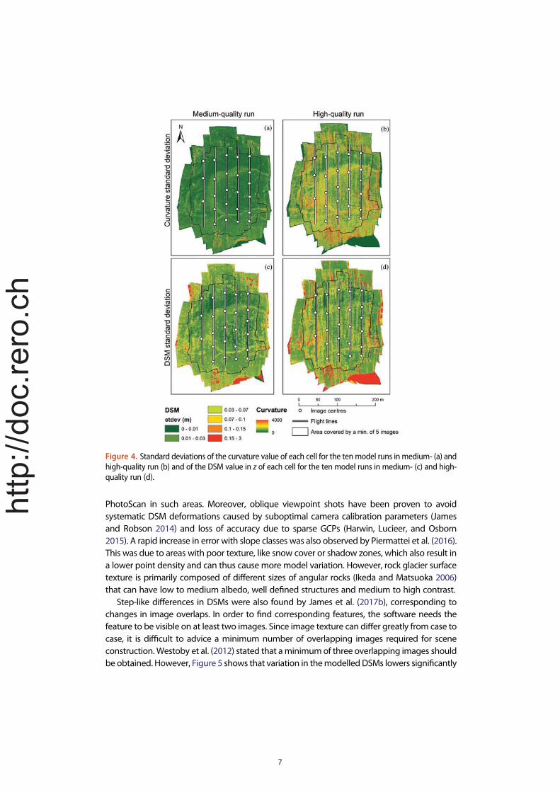
To quantify the variation within the output products (DSMs z-value and curvature) of thetenmodel runs, the standard deviation for each cell valuewas calculated (Figure 4). Both themedium- and high-quality runs showmore variation at the edges of the DSMs (10 cm – 3m)and curvature (3000 – 4000 within a range of [−80 000; +80 000]. This variation is due to lessGCPs and less overlapping images (Figure 5), resulting in a lower point density and thus ahigher model variation. The medium-quality run shows a clear pattern in variation withslope and surface roughness (Figure 4(a), (c); Figure 6), while the high-quality run has amorelinear pattern of variation, which seems related to the flight lines and the overlap areas ofthe images, for both DSM and curvature (Figure 4(b), (d); Figure 6). Comparing the pointclouds with the M3C2 algorithm in CloudCompare (Lague, Brodu, and Leroux 2013) givesthe same results, excluding the gridding process as cause of these model variations.

4. Discussion and conclusion

The variation between different PhotoScan model runs is relatively small, as shown by thevery small difference between the calculated coordinates and small RMSE (Table 1).Nevertheless, different PhotoScan model runs can give different outcome products (in thiscase point clouds, DSMs and calculated curvatures), although same input data and proces-sing details are used. The variation between DSMs is small and stays under the modelaccuracy for 88 to 96% of the study area (high- and medium-quality run respectively).However, in some cases the DSM variation is larger than the accuracy of the model itself(≥10 cm in z), whereas 3 to 6%of these variations lie at the edge of themodel (image overlap<5) and 1 to 6% lie within this boundary (high- and medium-quality run respectively).

DSM variation is clearly linked to slope gradient and surface roughness for the medium-quality run (Figure 4(c), Figure 6(c)). This is to be expected, since inaccuracies in x and yautomatically resolve in inaccuracy in z, especially on steep slopes and areas with a highsurface roughness. Curvature variation, as a measure on how well the model can reproducethe surface morphology, shows an even more pronounced relationship with slope gradient(Figure 4(a), Figure 6(a)). Standard deviations and thus variation in themodel result are largestin areas with high slope gradient and surface roughness. This is especially relevant forgeomorphic studies since process magnitude is higher on steep slopes, and model inaccura-cies on these location may mislead interpretations. It is, therefore, recommended to addoblique viewpoint flights to get a higher point density and a better reproducibility by

Table 1. Root Mean Square Errors (RMSE) of x, y and z to evaluate the overall model performance. Theaverage and the standard deviation of the tenmodel runs are presented for both medium and high qualityruns.

Medium High

Average (cm) Stdev (cm) Average (cm) Stdev (cm)

GCPs RMSE (x) 9.32 0.06 6.78 0.07RMSE (y) 2.50 0.01 4.52 0.18RMSE (z) 8.85 0.03 8.56 0.26

CPs RMSE (x) 11.84 0.07 10.95 0.08RMSE (y) 3.88 0.03 5.05 0.07RMSE (z) 9.96 0.20 9.27 0.19

6

http://doc.rero.ch

PhotoScan in such areas. Moreover, oblique viewpoint shots have been proven to avoidsystematic DSM deformations caused by suboptimal camera calibration parameters (Jamesand Robson 2014) and loss of accuracy due to sparse GCPs (Harwin, Lucieer, and Osborn2015). A rapid increase in error with slope classes was also observed by Piermattei et al. (2016).This was due to areas with poor texture, like snow cover or shadow zones, which also result ina lower point density and can thus cause more model variation. However, rock glacier surfacetexture is primarily composed of different sizes of angular rocks (Ikeda and Matsuoka 2006)that can have low to medium albedo, well defined structures and medium to high contrast.

Step-like differences in DSMs were also found by James et al. (2017b), corresponding tochanges in image overlaps. In order to find corresponding features, the software needs thefeature to be visible on at least two images. Since image texture can differ greatly from case tocase, it is difficult to advice a minimum number of overlapping images required for sceneconstruction.Westoby et al. (2012) stated that aminimumof three overlapping images shouldbe obtained. However, Figure 5 shows that variation in themodelledDSMs lowers significantly

Figure 4. Standard deviations of the curvature value of each cell for the tenmodel runs inmedium- (a) andhigh-quality run (b) and of the DSM value in z of each cell for the ten model runs in medium- (c) and high-quality run (d).

7

http://doc.rero.ch

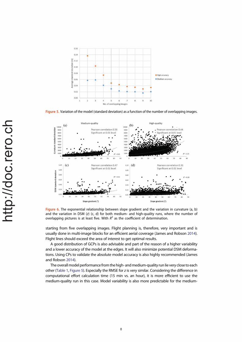
starting from five overlapping images. Flight planning is, therefore, very important and isusually done in multi-image blocks for an efficient aerial coverage (James and Robson 2014).Flight lines should exceed the area of interest to get optimal results.

A good distribution of GCPs is also advisable and part of the reason of a higher variabilityand a lower accuracy of the model at the edges. It will also minimize potential DSM deforma-tions. Using CPs to validate the absolute model accuracy is also highly recommended (Jamesand Robson 2014).

Theoverallmodelperformance fromthehigh-andmedium-quality run lieveryclose toeachother (Table 1, Figure 5). Especially the RMSE for z is very similar. Considering the difference incomputational effort calculation time (15 min vs. an hour), it is more efficient to use themedium-quality run in this case. Model variability is also more predictable for the medium-

Figure 6. The exponential relationship between slope gradient and the variation in curvature (a, b)and the variation in DSM (z) (c, d) for both medium- and high-quality runs, where the number ofoverlapping pictures is at least five. With R2 as the coefficient of determination.

Figure 5. Variation of the model (standard deviation) as a function of the number of overlapping images.

8

http://doc.rero.ch

quality run, since it is more clearly linked to slope steepness. Moreover, both variations in DSM(z) and curvature show a better performance using the medium-quality run (Figure 6).

From the above we can conclude that PhotoScan is reliable software to perform highresolution processing of SfM-MVS data and that it can reproduce the same outcome with aminimum of variation, even in a complex topography. However, the model varies more at themodel edges and in areas with pronounced/complex relief. Especially the latter may biasgeomorphic interpretations. These variations canbeminimizedby usingmedium-quality runs,additional oblique viewpoints and realizing aminimumof five overlapping images. Therefore,good planning is crucial, especially when surveying large and complex terrain.

Acknowledgments

Adeline Frossard (Msc student UNIL) is thanked for her help during the field work. Field logistics wereorganized by IDYST-UNIL. The authors thank the anonymous reviewer for valuable comments.

External links

3D Model of this experiment: https://skfb.ly/6uM6wEntire 3D model of the site: https://skfb.ly/6uNzZ

Disclosure statement

No potential conflict of interest was reported by the authors

Funding

H. Hendrickx’s field stay was funded by Research Foundations – Flanders under a travel grant(V4.321.17N) for long research stay abroad.

ORCID

Sebastián Vivero http://orcid.org/0000-0002-1813-9575Philippe De Maeyer http://orcid.org/0000-0001-8902-3855

References

Agisoft. 2018. “Agisoft PhotoScan User Manual.” Professional Edition, Version 1.4. http://www.agisoft.com/downloads/user-manuals/

Dall’Asta, E., G. Forlani, R. Roncella, M. Santise, F. Diotri, and U. Morra Di Cella. 2017. “UnmannedAerial Systems and DSM Matching for Rock Glacier Monitoring.” ISPRS Journal ofPhotogrammetry and Remote Sensing 127: 102–114. doi:10.1016/j.isprsjprs.2016.10.003.

Delaloye, R., C. Lambiel, and G.-R. Isabelle. 2010. “Overview of Rock Glacier Kinematics Research inthe Swiss Alps: Seasonal Rhythm, Interannual Variations and Trends over Several Decades.”Geographica Helvetica 65 (2): 135–145. doi:10.5194/gh-65-135-2010.

Fonstad, M. A., J. T. Dietrich, B. C. Courville, J. L. Jensen, and P. E. Carbonneau. 2013. “TopographicStructure from Motion: A New Development in Photogrammetric Measurement.” Earth SurfaceProcesses and Landforms. doi:10.1002/esp.3366.

Frankl, A., C. Stal, A. Abraha, J. Nyssen, D. Rieke-Zapp, A. DeWulf, and J. Poesen. 2015. “Detailed Recordingof GullyMorphology in 3D through Image-BasedModelling.” CATENA 127 (April): 92–101. doi:10.1016/j.catena.2014.12.016.

9

http://doc.rero.ch

Harwin, S., and A. Lucieer. 2012. “Assessing the Accuracy of Georeferenced Point Clouds Produced viaMulti-View Stereopsis from Unmanned Aerial Vehicle (UAV) Imagery.” Remote Sensing 4 (6): 1573–1599. doi:10.3390/rs4061573.

Harwin, S., A. Lucieer, and J. Osborn. 2015. “The Impact of the Calibration Method on the Accuracyof Point Clouds Derived Using Unmanned Aerial Vehicle Multi-View Stereopsis.” Remote Sensing7 (9): 11933–11953. doi:10.3390/rs70911933.

Ikeda, A., and N. Matsuoka. 2006. “Pebbly versus Bouldery Rock Glaciers: Morphology, Structureand Processes.” Geomorphology 73 (3–4): 279–296. doi:10.1016/j.geomorph.2005.07.015.

James, M. R., and S. Robson. 2014. “Mitigating Systematic Error in Topographic Models Derivedfrom UAV and Ground-Based Image Networks.” Earth Surface Processes and Landforms 39 (10):1413–1420. doi:10.1002/esp.3609.

James, M. R., S. Stuart Robson, S. D’Oleire-Oltmanns, and U. Niethammer. 2017a. “Optimising UAVTopographic Surveys Processed with Structure-from-Motion: Ground Control Quality, Quantityand Bundle Adjustment.” Geomorphology 280: 51–66. doi:10.1016/j.geomorph.2016.11.021.

James, M. R., S. Robson, andM. W. Smith. 2017b. “3-D Uncertainty-Based Topographic Change Detectionwith Structure-from-Motion Photogrammetry: Precision Maps for Ground Control and DirectlyGeoreferenced Surveys.” Earth Surface Processes and Landforms 42 (12): 1769–1788. doi:10.1002/esp.4125.

Javernick, L., J. Brasington, and B. Caruso. 2014. “Modeling the Topography of Shallow Braided RiversUsing Structure-from-Motion Photogrammetry.” Geomorphology 213: 166–182. doi:10.1016/j.geomorph.2014.01.006.

Kenner, R., M. Phillips, C. Hauck, C. Hilbich, C. Mulsow, Y. Bühler, A. Stoffel, and M. Buchroithner. 2017.“New Insights on Permafrost Genesis and Conservation in Talus Slopes Based on Observations atFlüelapass, Eastern Switzerland.” Geomorphology 290: 101–113. doi:10.1016/j.geomorph.2017.04.011.

Lague, D., N. Brodu, and J. Leroux. 2013. “Accurate 3D Comparison of Complex Topography withTerrestrial Laser Scanner: Application to the Rangitikei Canyon (N-Z).” ISPRS Journal ofPhotogrammetry and Remote Sensing 82: 10–26. International Society for Photogrammetry andRemote Sensing, Inc. (ISPRS). doi:10.1016/j.isprsjprs.2013.04.009.

Lannoeye, W., C. Stal, E. Guyassa, A. Zenebe, J. Nyssen, and A. Frankl. 2016. “The Use of SfM-Photogrammetry to Quantify and Understand Gully Degradation at the Temporal Scale ofRainfall Events: An Example from the Ethiopian Drylands.” Physical Geography 37 (6): 430–451.doi:10.1080/02723646.2016.1234197.

Lowe, D. G. 2004. “Distinctive Image Features from Scale-Invariant Keypoints.” International Journalof Computer Vision 60 (2): 91–110. doi:10.1023/B:VISI.0000029664.99615.94.

Niethammer, U., M. R. James, S. Rothmund, J. Travelletti, and M. Joswig. 2012. “UAV-Based RemoteSensing of the Super-Sauze Landslide: Evaluation and Results.” Engineering Geology 128: 2–11.doi:10.1016/j.enggeo.2011.03.012.

Piermattei, L., L. Carturan, F. De Blasi, P. Tarolli, G. D. Fontana, A. Vettore, and N. Pfeifer. 2016.“Suitability of Ground-Based SfM-MVS for Monitoring Glacial and Periglacial Processes.” EarthSurface Dynamics 4 (2): 425–443. doi:10.5194/esurf-4-425-2016.

Semyonov, D. 2011. “Algorithms Used in Photoscan [Msg 2].” www.agisoft.ru/forum/index.php?topic=89.0

Smith, M. W., J. L. Carrivick, and D. J. Quincey. 2015. “Structure from Motion Photogrammetry in PhysicalGeography.” Progress in Physical Geography 40 (2): 247–275. doi:10.1177/0309133315615805.

Uysal, M., A. S. Toprak, and N. Polat. 2015. “DEM Generation with UAV Photogrammetry andAccuracy Analysis in Sahitler Hill.” Measurement: Journal of the International MeasurementConfederation 73: 539–543. doi:10.1016/j.measurement.2015.06.010.

Westoby, M. J., J. Brasington, N. F. Glasser, M. J. Hambrey, and J. M. Reynolds. 2012. “‘Structure-From-Motion’ Photogrammetry: A Low-Cost, Effective Tool for Geoscience Applications.”Geomorphology 179: 300–314. doi:10.1016/j.geomorph.2012.08.021.

Zevenbergen, L. W., and C. R. Thorne. 1987. “Quantitative Analysis of Land Surface Topography.”Earth Surface Processes and Landforms 12 (1): 47–56. doi:10.1002/esp.3290120107.

10

http://doc.rero.ch