university of illinois at urbana-champaign … 1/2012 university of illinois at urbana-champaign...
TRANSCRIPT
Revised 1/2012
University of Illinois at Urbana-Champaign Department of Physics
Physics 401 Classical Physics Laboratory
Experiment 5
Transients and Oscillations in RLC Circuits
I. Introduction ................................................................................................................................. 2
II. Theory ........................................................................................................................................ 3
A. Over-damped solution 2 0b ........................................................................................ 5
B. Critically damped solution 2 0b .................................................................................. 5
C. Under-damped solution 2 0b ...................................................................................... 6
III. Practical capacitors and inductors ............................................................................................. 8
A. Determine dependence of frequency on capacitance .................................................. 10
B. Determine the dependence of log decrement on resistance ........................................ 12
C. Determine the value of resistance for critical damping............................................... 13
D. Measure the response of an RLC circuit to a sinusoidal signal .................................. 15
V. Report ....................................................................................................................................... 20
Appendix I. Derivation of the series RLC equation and basic circuit analysis ........................... 21
Physics 401 Experiment 5 Page Transients in RLC Circuits 2/23
I. Introduction
In this experiment we first study the behavior of transients in a series RLC circuit as we vary the
resistance and the capacitance. We find that two qualitatively different transients are possible, a
damped oscillation and an exponential decay. We then drive the RLC circuit with an external
sinusoidal voltage and find that the response of the circuit depends on the driving frequency. We
find that the response of the circuit shows maximum at some particular frequency. We compare
our observations to a simple model.
A wide variety of physical systems are understood as examples of oscillating systems: the simple
pendulum, the mass on a spring, the charged particle in a storage ring, and the series RLC circuit.
In each of these physical systems we determine how a single variable, for example, the position
of the mass on the spring or the charge on the capacitor, changes with time. There are many
elements common to the description of all oscillating systems. For example, all of these systems
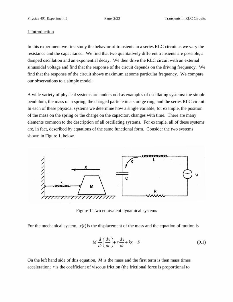
are, in fact, described by equations of the same functional form. Consider the two systems
shown in Figure 1, below.
Figure 1 Two equivalent dynamical systems
For the mechanical system, ( )x t is the displacement of the mass and the equation of motion is
d dx dx
M r kx Fdt dt dt
(0.1)
On the left hand side of this equation, M is the mass and the first term is then mass times
acceleration; r is the coefficient of viscous friction (the frictional force is proportional to
V
Physics 401 Experiment 5 Page Transients in RLC Circuits 3/23
velocity1); and k is the spring constant (the spring force is kx ). On the right-hand side of the
equation, F represents an external driving force (not shown in the figure).
For the RLC circuit, q t is the charge on the capacitor, and Kirchoff’s voltage law (see
Appendix I for a very brief exposition of Kirchoff’s laws) gives the equation
1d dq dq
L R q V tdt dt dt C
(0.2)
On the left-hand side of the equation, the first term is the voltage drop across the inductor. We
have used the derivative of the charge on the capacitor for the current through the inductor. The
second term is the voltage drop across the resistor, and the third term is the voltage drop across
the capacitor. On the right-hand side V t is an externally applied voltage. We find in
comparing Equation (0.1) and Equation (0.2) that the mass behaves the same as an inductor, and
the spring the same as an inverse capacitance. Displacement becomes charge, and the viscous
friction is replaced by a resistor. Such correspondences can be found in other systems.
The theory below first treats the case in which there is no externally applied voltage. The
solution has two qualitatively different forms. Several important quantities are defined: natural
(angular) frequency for oscillation, o
, the quality factor, Q , and the logarithmic decrement, ,
which is also called the log decrement. The logarithm has the base e , but no one ever calls the
ln decrement. The concept of critical damping is also introduced. The case in which there is an
externally applied sinusoidal voltage is discussed only briefly. The concept of resonance is
introduced.
II. Theory
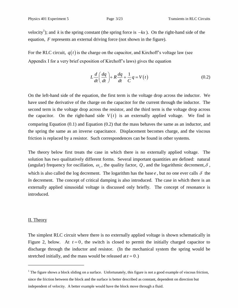
The simplest RLC circuit where there is no externally applied voltage is shown schematically in
Figure 2, below. At 0t , the switch is closed to permit the initially charged capacitor to
discharge through the inductor and resistor. (In the mechanical system the spring would be
stretched initially, and the mass would be released at 0t .)
1 The figure shows a block sliding on a surface. Unfortunately, this figure is not a good example of viscous friction,
since the friction between the block and the surface is better described as constant, dependent on direction but
independent of velocity. A better example would have the block move through a fluid.
Physics 401 Experiment 5 Page Transients in RLC Circuits 4/23
Figure 2 RLC circuit with voltage on capacitor initially
Application of Kirchhoff’s law gives
0d dq dq q
L Rdt dt dt C
, (0.3)
where dq
dtis the current. This equation is a homogeneous, linear, second-order differential
equation and has solutions of the form stq t Ae , where A is an arbitrary constant.
Substituting this function into Equation (0.2) produces a quadratic equation for s :
2 10
Rs s
L LC
, (0.4)
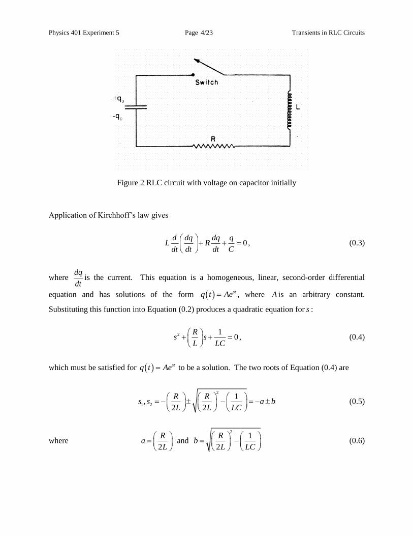
which must be satisfied for stq t Ae to be a solution. The two roots of Equation (0.4) are
2
1 2
1,
2 2
R Rs s a b
L L LC
(0.5)
where 2
Ra
L
and
21
2
Rb
L LC
(0.6)
Physics 401 Experiment 5 Page Transients in RLC Circuits 5/23
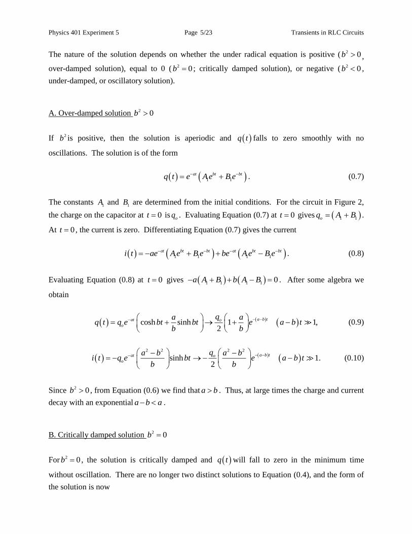
The nature of the solution depends on whether the under radical equation is positive ( 2 0b ,
over-damped solution), equal to 0 ( 2 0b ; critically damped solution), or negative ( 2 0b ,
under-damped, or oscillatory solution).
A. Over-damped solution 2 0b
If 2b is positive, then the solution is aperiodic and q t falls to zero smoothly with no
oscillations. The solution is of the form
1 1
at bt btq t e A e B e . (0.7)
The constants 1
A and 1
B are determined from the initial conditions. For the circuit in Figure 2,
the charge on the capacitor at 0t iso
q . Evaluating Equation (0.7) at 0t gives 1 1oq A B .
At 0t , the current is zero. Differentiating Equation (0.7) gives the current
1 1 1 1
at bt bt at bt bti t ae A e B e be A e B e . (0.8)
Evaluating Equation (0.8) at 0t gives 1 1 1 10a A B b A B . After some algebra we
obtain
cosh sinh 1 1,2
a b tat o
o
qa aq t q e bt bt e a b t
b b
(0.9)
2 2 2 2
sinh 1.2
a b tat o
o
qa b a bi t q e bt e a b t
b b
(0.10)
Since 2 0b , from Equation (0.6) we find that a b . Thus, at large times the charge and current
decay with an exponential a b a .
B. Critically damped solution 2 0b
For 2 0b , the solution is critically damped and q t will fall to zero in the minimum time
without oscillation. There are no longer two distinct solutions to Equation (0.4), and the form of
the solution is now
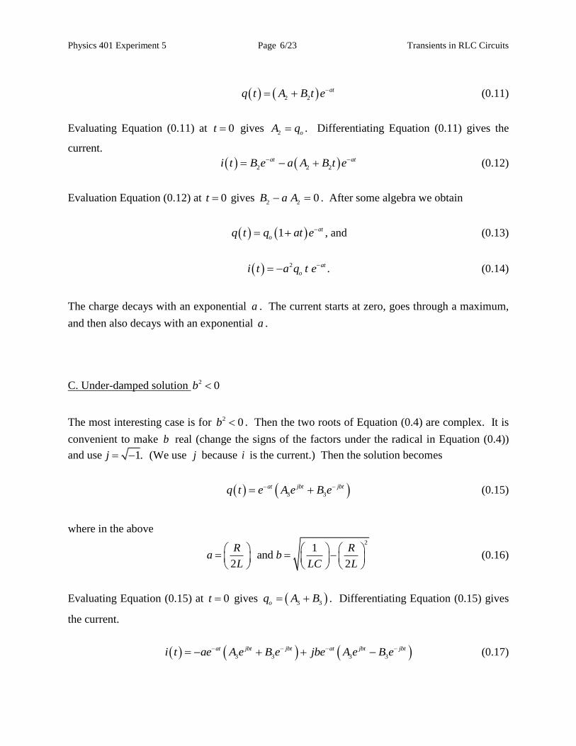
Physics 401 Experiment 5 Page Transients in RLC Circuits 6/23
2 2
atq t A B t e (0.11)
Evaluating Equation (0.11) at 0t gives 2 o
A q . Differentiating Equation (0.11) gives the
current.
2 2 2
at ati t B e a A B t e (0.12)
Evaluation Equation (0.12) at 0t gives 2 2
0B a A . After some algebra we obtain
1 at
oq t q at e , and (0.13)
2 .at
oi t a q t e (0.14)
The charge decays with an exponential a . The current starts at zero, goes through a maximum,
and then also decays with an exponential a .
C. Under-damped solution 2 0b
The most interesting case is for 2 0b . Then the two roots of Equation (0.4) are complex. It is
convenient to make b real (change the signs of the factors under the radical in Equation (0.4))
and use 1.j (We use j because i is the current.) Then the solution becomes
3 3
at jbt jbtq t e A e B e (0.15)
where in the above
21
and 2 2
R Ra b
L LC L
(0.16)
Evaluating Equation (0.15) at 0t gives 3 3oq A B . Differentiating Equation (0.15) gives
the current.
3 3 3 3
at jbt jbt at jbt jbti t ae A e B e jbe A e B e (0.17)
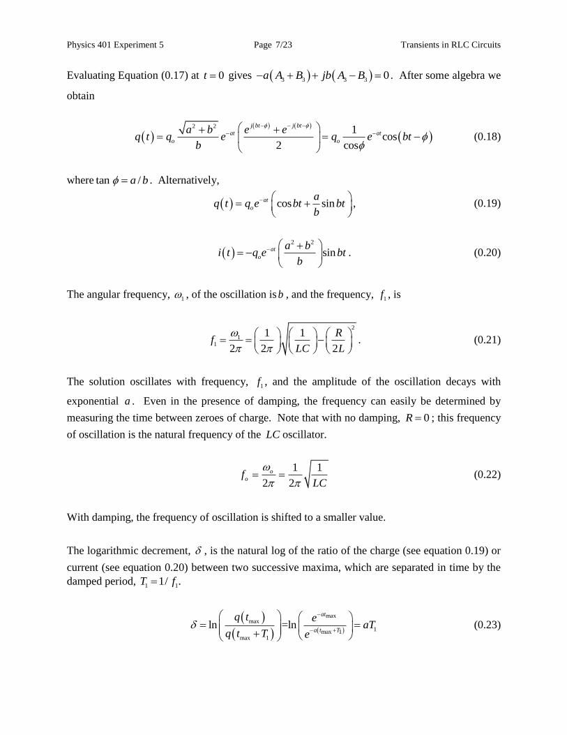
Physics 401 Experiment 5 Page Transients in RLC Circuits 7/23
Evaluating Equation (0.17) at 0t gives 3 3 3 30a A B jb A B . After some algebra we
obtain
2 2 1
cos2 cos
j bt j bt
at at
o o
a b e eq t q e q e bt
b
(0.18)
where tan /a b . Alternatively,
cos sinat
o
aq t q e bt bt
b
, (0.19)
2 2
sinat
o
a bi t q e bt
b
. (0.20)
The angular frequency, 1
, of the oscillation is b , and the frequency, 1
f , is
2
1
1
1 1
2 2 2
Rf
LC L
. (0.21)
The solution oscillates with frequency, 1
f , and the amplitude of the oscillation decays with
exponential a . Even in the presence of damping, the frequency can easily be determined by
measuring the time between zeroes of charge. Note that with no damping, 0R ; this frequency
of oscillation is the natural frequency of the LC oscillator.
1 1
2 2
o
of
LC
(0.22)
With damping, the frequency of oscillation is shifted to a smaller value.
The logarithmic decrement, , is the natural log of the ratio of the charge (see equation 0.19) or
current (see equation 0.20) between two successive maxima, which are separated in time by the
damped period, 1 1
1/ .T f
maxmax
1max 1max 1
ln =lnat
a t T
q t eaT
q t T e
(0.23)
Physics 401 Experiment 5 Page Transients in RLC Circuits 8/23
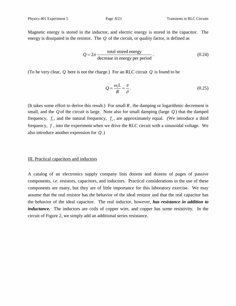
Magnetic energy is stored in the inductor, and electric energy is stored in the capacitor. The
energy is dissipated in the resistor. The Q of the circuit, or quality factor, is defined as
total stored energy
2decrease in energy per period
Q . (0.24)
(To be very clear, Q here is not the charge.) For an RLC circuit Q is found to be
1L
QR
. (0.25)
(It takes some effort to derive this result.) For small R , the damping or logarithmic decrement is
small, and the Q of the circuit is large. Note also for small damping (large Q ) that the damped
frequency, 1
f , and the natural frequency, o
f , are approximately equal. (We introduce a third
frequency, f , into the experiment when we drive the RLC circuit with a sinusoidal voltage. We
also introduce another expression for Q .)
III. Practical capacitors and inductors
A catalog of an electronics supply company lists dozens and dozens of pages of passive
components, i.e. resistors, capacitors, and inductors. Practical considerations in the use of these
components are many, but they are of little importance for this laboratory exercise. We may
assume that the real resistor has the behavior of the ideal resistor and that the real capacitor has
the behavior of the ideal capacitor. The real inductor, however, has resistance in addition to
inductance. The inductors are coils of copper wire, and copper has some resistivity. In the
circuit of Figure 2, we simply add an additional series resistance.
Physics 401 Experiment 5 Page Transients in RLC Circuits 9/23
Rout R L
C
Wavetek
VC
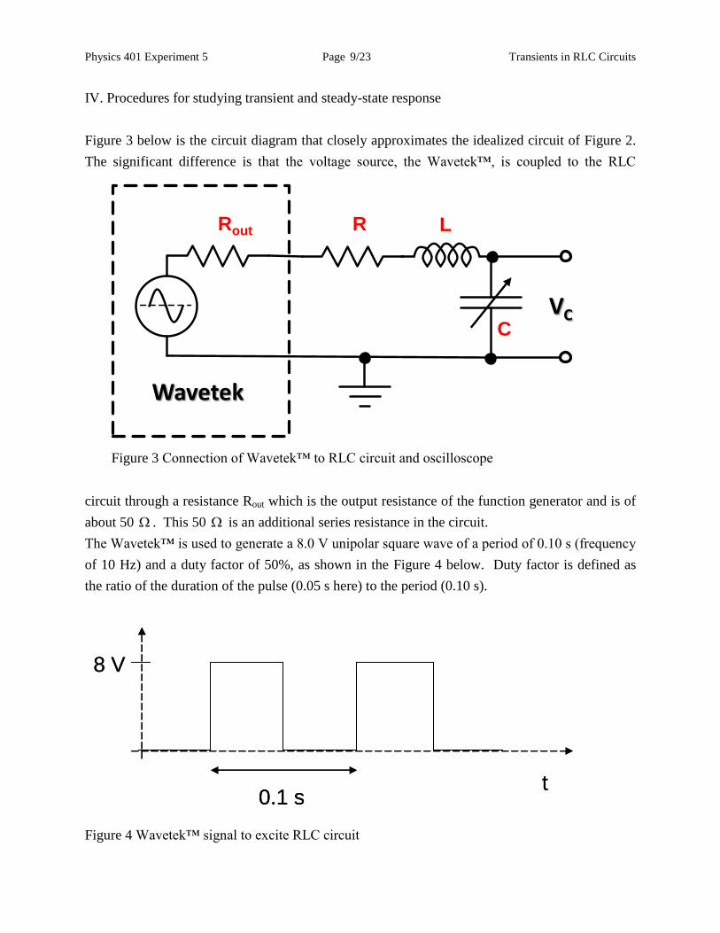
Figure 3 Connection of Wavetek™ to RLC circuit and oscilloscope
IV. Procedures for studying transient and steady-state response
Figure 3 below is the circuit diagram that closely approximates the idealized circuit of Figure 2.
The significant difference is that the voltage source, the Wavetek™, is coupled to the RLC
circuit through a resistance Rout which is the output resistance of the function generator and is of
about 50 . This 50 is an additional series resistance in the circuit.
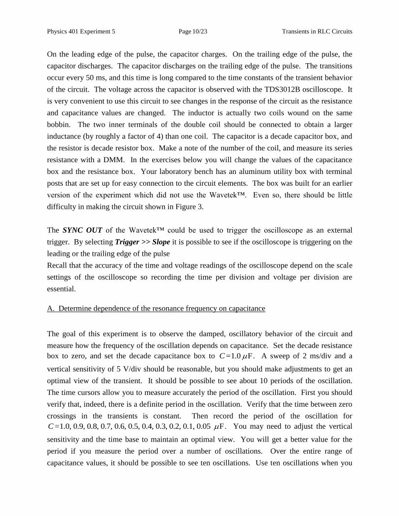
The Wavetek™ is used to generate a 8.0 V unipolar square wave of a period of 0.10 s (frequency
of 10 Hz) and a duty factor of 50%, as shown in the Figure 4 below. Duty factor is defined as
the ratio of the duration of the pulse (0.05 s here) to the period (0.10 s).
0.1 s
8 V
Signal from Wavetek
t0.1 s
8 V
Signal from Wavetek
t
Figure 4 Wavetek™ signal to excite RLC circuit
Physics 401 Experiment 5 Page Transients in RLC Circuits 10/23
On the leading edge of the pulse, the capacitor charges. On the trailing edge of the pulse, the
capacitor discharges. The capacitor discharges on the trailing edge of the pulse. The transitions
occur every 50 ms, and this time is long compared to the time constants of the transient behavior
of the circuit. The voltage across the capacitor is observed with the TDS3012B oscilloscope. It
is very convenient to use this circuit to see changes in the response of the circuit as the resistance
and capacitance values are changed. The inductor is actually two coils wound on the same
bobbin. The two inner terminals of the double coil should be connected to obtain a larger
inductance (by roughly a factor of 4) than one coil. The capacitor is a decade capacitor box, and
the resistor is decade resistor box. Make a note of the number of the coil, and measure its series
resistance with a DMM. In the exercises below you will change the values of the capacitance
box and the resistance box. Your laboratory bench has an aluminum utility box with terminal
posts that are set up for easy connection to the circuit elements. The box was built for an earlier
version of the experiment which did not use the Wavetek™. Even so, there should be little
difficulty in making the circuit shown in Figure 3.
The SYNC OUT of the Wavetek™ could be used to trigger the oscilloscope as an external
trigger. By selecting Trigger >> Slope it is possible to see if the oscilloscope is triggering on the
leading or the trailing edge of the pulse
Recall that the accuracy of the time and voltage readings of the oscilloscope depend on the scale
settings of the oscilloscope so recording the time per division and voltage per division are
essential.
A. Determine dependence of the resonance frequency on capacitance
The goal of this experiment is to observe the damped, oscillatory behavior of the circuit and
measure how the frequency of the oscillation depends on capacitance. Set the decade resistance
box to zero, and set the decade capacitance box to =1.0 FC . A sweep of 2 ms/div and a
vertical sensitivity of 5 V/div should be reasonable, but you should make adjustments to get an
optimal view of the transient. It should be possible to see about 10 periods of the oscillation.
The time cursors allow you to measure accurately the period of the oscillation. First you should
verify that, indeed, there is a definite period in the oscillation. Verify that the time between zero
crossings in the transients is constant. Then record the period of the oscillation for
=1.0, 0.9, 0.8, 0.7, 0.6, 0.5, 0.4, 0.3, 0.2, 0.1, 0.05 FC . You may need to adjust the vertical
sensitivity and the time base to maintain an optimal view. You will get a better value for the
period if you measure the period over a number of oscillations. Over the entire range of
capacitance values, it should be possible to see ten oscillations. Use ten oscillations when you
Physics 401 Experiment 5 Page Transients in RLC Circuits 11/23
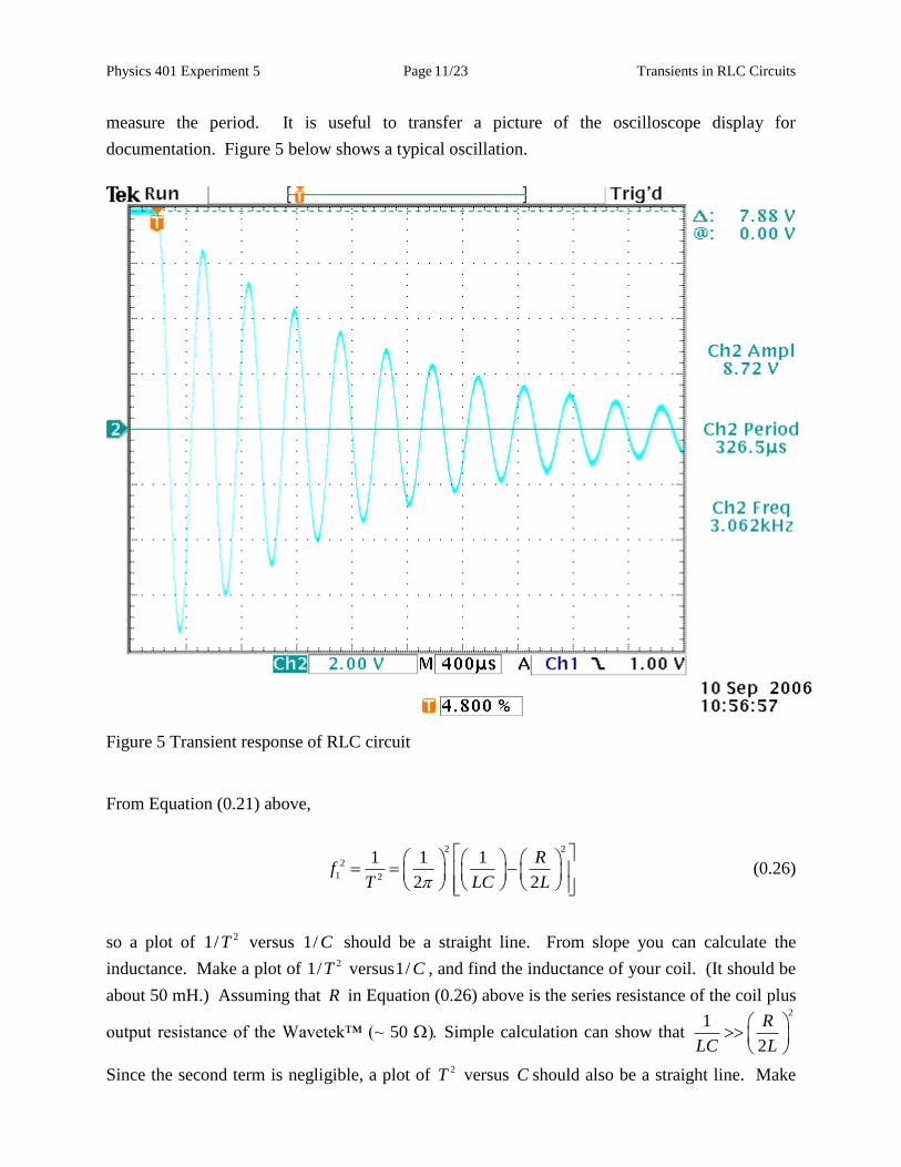
measure the period. It is useful to transfer a picture of the oscilloscope display for
documentation. Figure 5 below shows a typical oscillation.
Figure 5 Transient response of RLC circuit
From Equation (0.21) above,
2 2
2
1 2
1 1 1
2 2
Rf
T LC L
(0.26)
so a plot of 21/T versus 1/ C should be a straight line. From slope you can calculate the
inductance. Make a plot of 21/T versus1/ C , and find the inductance of your coil. (It should be
about 50 mH.) Assuming that R in Equation (0.26) above is the series resistance of the coil plus
output resistance of the Wavetek™ (~ 50 Simple calculation can show that
21
2
R
LC L
Since the second term is negligible, a plot of 2T versus C should also be a straight line. Make
Physics 401 Experiment 5 Page Transients in RLC Circuits 12/23
this plot (and the other plots described below) with Excel as you take the data. Print a copy to
paste in your notebook.
22 2T LC (0.27)
An impedance meter is available in the laboratory, the Z-meter, which can measure inductances
and capacitances. Find the meter, read the brief instructions, and measure the inductance of your
coil. Compare the measured inductance with those obtained from slope.
B. Determine the dependence of log decrement on resistance
The goal of this part of the exercise is to find how the rate of damping of the transient depends
on the resistance. With C = 1.0 F increase the resistance of the decade resistance box, R ,
from zero to 300 in large steps 50 while you observe the oscillating transient. Again you
will need to adjust the horizontal sweep and vertical sensitivity to get an optimal view. At what
resistance do you find it difficult to see more than one or two strongly damped oscillations? Use
the H Bar cursors of the oscilloscope to measure the amplitudes of the peaks of the transient. If
the amplitude of the first positive peak is V1 and the second positive peak is V2, the log
decrement is log 1/ 2V V . For = 0R , verify that the log decrement is, indeed, a constant
by measuring the voltage ratio for a few adjacent positive peaks, say, V1/V2, V2/V3, V3/V4,
V4/V5. Since these ratios are constant, you will get a better measurement for the log decrement
if you measure it between several oscillations. However, it is also possible to adjust the vertical
sensitivity of the oscilloscope to get a good measurement of the log decrement just between
adjacent peaks. When changing the value of R you should also note that the period changes, but
only slowly. For =100, 90, 80, 70, 60, 50, 40, 30, 10, 0 R , measure the log decrement of the
transient.
From (0.24).
2 2
2 1
2 2 1 142
R R R CaT T LC R
L L L LR CR
LLC L
. (0.28)
If the period does not change much (equivalently, if 2 / 4 1R C L ), a plot of log decrement
versus R then should be a straight line. Make a plot log decrement versus R and note that the
Physics 401 Experiment 5 Page Transients in RLC Circuits 13/23
line does not pass through the origin. The offset is due to additional resistance in the circuit, for
example, the resistance of the coil plus output resistance of the Wavetek™ (~50 ). Determine
the effective additional resistance in the circuit from the zero intercept of your plot.
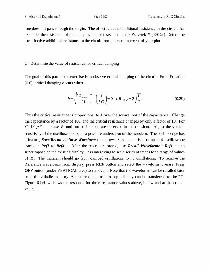
C. Determine the value of resistance for critical damping
The goal of this part of the exercise is to observe critical damping of the circuit. From Equation
(0.6), critical damping occurs when
21
0 2 .2
critical
critical
R Lb R
L LC C
(0.29)
Thus the critical resistance is proportional to 1 over the square root of the capacitance. Change
the capacitance by a factor of 100, and the critical resistance changes by only a factor of 10. For
C=1.0 F , increase R until no oscillations are observed in the transient. Adjust the vertical
sensitivity of the oscilloscope to see a possible undershoot of the transient. The oscilloscope has
a feature, Save/Recall >> Save Waveform that allows easy comparison of up to 4 oscilloscope
traces in Ref1 to Ref4. After the traces are stored, use Recall Waveform>> Ref1 etc to
superimpose on the existing display. It is interesting to see a series of traces for a range of values
of R . The transient should go from damped oscillations to no oscillations. To remove the
Reference waveforms from display, press REF button and select the waveform to erase. Press
OFF button (under VERTICAL area) to remove it. Note that the waveforms can be recalled later
from the volatile memory. A picture of the oscilloscope display can be transferred to the PC.
Figure 6 below shows the response for three resistance values above, below and at the critical
value.
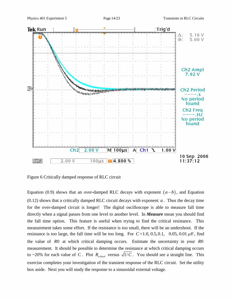
Physics 401 Experiment 5 Page Transients in RLC Circuits 14/23
Figure 6 Critically damped response of RLC circuit
Equation (0.9) shows that an over-damped RLC decays with exponent a b , and Equation
(0.12) shows that a critically damped RLC circuit decays with exponent a . Thus the decay time
for the over-damped circuit is longer! The digital oscilloscope is able to measure fall time
directly when a signal passes from one level to another level. In Measure mean you should find
the fall time option. This feature is useful when trying to find the critical resistance. This
measurement takes some effort. If the resistance is too small, there will be an undershoot. If the
resistance is too large, the fall time will be too long. For =1.0, 0.5,0.1, C 0.05, 0.01 F , find
the value of 0R at which critical damping occurs. Estimate the uncertainty in your 0R
measurement. It should be possible to determine the resistance at which critical damping occurs
to ~20% for each value of C . Plot critical
R versus 1/ C . You should see a straight line. This
exercise completes your investigation of the transient response of the RLC circuit. Set the utility
box aside. Next you will study the response to a sinusoidal external voltage.
Physics 401 Experiment 5 Page Transients in RLC Circuits 15/23
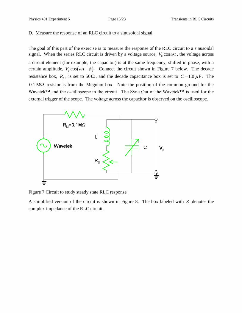
D. Measure the response of an RLC circuit to a sinusoidal signal
The goal of this part of the exercise is to measure the response of the RLC circuit to a sinusoidal
signal. When the series RLC circuit is driven by a voltage source, 0
cosV t , the voltage across
a circuit element (for example, the capacitor) is at the same frequency, shifted in phase, with a
certain amplitude, cosc
V t . Connect the circuit shown in Figure 7 below. The decade
resistance box, B
R , is set to 50 , and the decade capacitance box is set to 1.0 FC . The
0.1 M resistor is from the Megohm box. Note the position of the common ground for the
Wavetek™ and the oscilloscope in the circuit. The Sync Out of the Wavetek™ is used for the
external trigger of the scope. The voltage across the capacitor is observed on the oscilloscope.
Figure 7 Circuit to study steady state RLC response
A simplified version of the circuit is shown in Figure 8. The box labeled with Z denotes the
complex impedance of the RLC circuit.
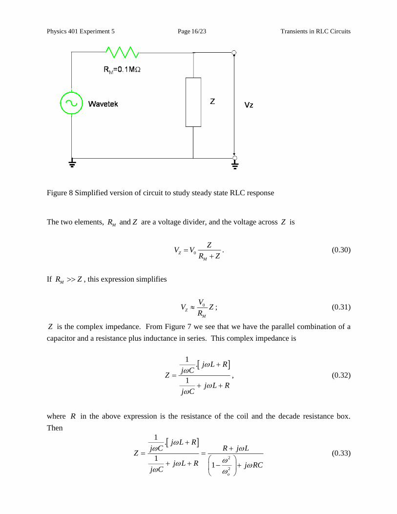
Physics 401 Experiment 5 Page Transients in RLC Circuits 16/23
Figure 8 Simplified version of circuit to study steady state RLC response
The two elements, and M
R Z are a voltage divider, and the voltage across Z is
0Z
M
ZV V
R Z
. (0.30)
If M
R Z , this expression simplifies
0
Z
M
VV Z
R ; (0.31)
Z is the complex impedance. From Figure 7 we see that we have the parallel combination of a
capacitor and a resistance plus inductance in series. This complex impedance is
1
.
1
j L Rj C
Z
j L Rj C
, (0.32)
where R in the above expression is the resistance of the coil and the decade resistance box.
Then
2
2
1.
11
o
j L RR j Lj C
Z
j L R j RCj C
(0.33)
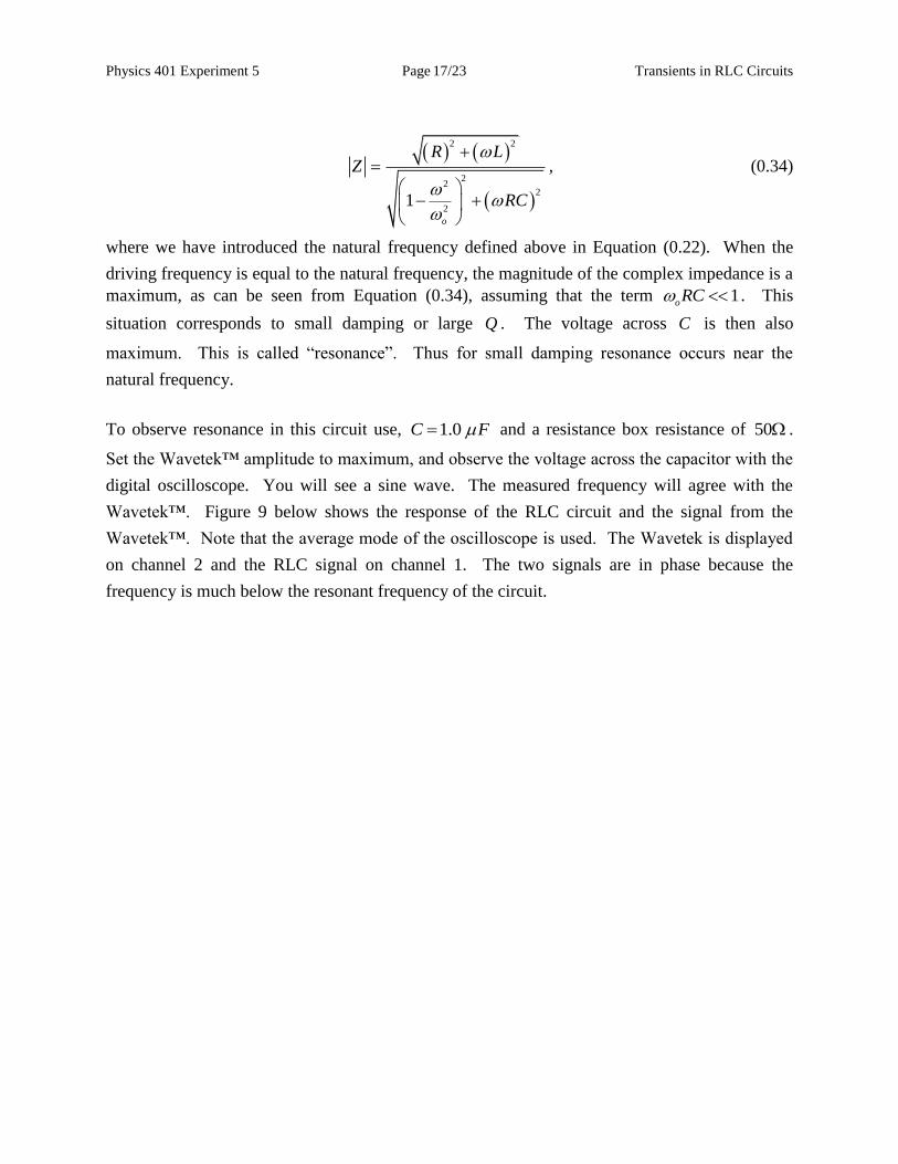
Physics 401 Experiment 5 Page Transients in RLC Circuits 17/23
2 2
22
2
21
o
R LZ
RC
, (0.34)
where we have introduced the natural frequency defined above in Equation (0.22). When the
driving frequency is equal to the natural frequency, the magnitude of the complex impedance is a
maximum, as can be seen from Equation (0.34), assuming that the term 1oRC . This
situation corresponds to small damping or large Q . The voltage across C is then also
maximum. This is called “resonance”. Thus for small damping resonance occurs near the
natural frequency.
To observe resonance in this circuit use, 1.0 C F and a resistance box resistance of 50 .
Set the Wavetek™ amplitude to maximum, and observe the voltage across the capacitor with the
digital oscilloscope. You will see a sine wave. The measured frequency will agree with the
Wavetek™. Figure 9 below shows the response of the RLC circuit and the signal from the
Wavetek™. Note that the average mode of the oscilloscope is used. The Wavetek is displayed
on channel 2 and the RLC signal on channel 1. The two signals are in phase because the
frequency is much below the resonant frequency of the circuit.
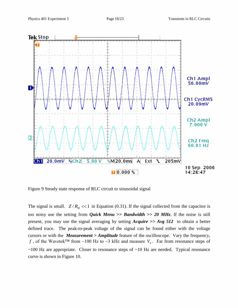
Physics 401 Experiment 5 Page Transients in RLC Circuits 18/23
Figure 9 Steady state response of RLC circuit to sinusoidal signal
The signal is small. / 1M
Z R in Equation (0.31). If the signal collected from the capacitor is
too noisy use the setting from Quick Menu >> Bandwidth >> 20 MHz. If the noise is still
present, you may use the signal averaging by setting Acquire >> Avg 512 to obtain a better
defined trace. The peak-to-peak voltage of the signal can be found either with the voltage
cursors or with the Measurement > Amplitude feature of the oscilloscope. Vary the frequency,
f , of the Wavetek™ from ~100 Hz to ~3 kHz and measure Z
V . Far from resonance steps of
~100 Hz are appropriate. Closer to resonance steps of ~10 Hz are needed. Typical resonance
curve is shown in Figure 10.
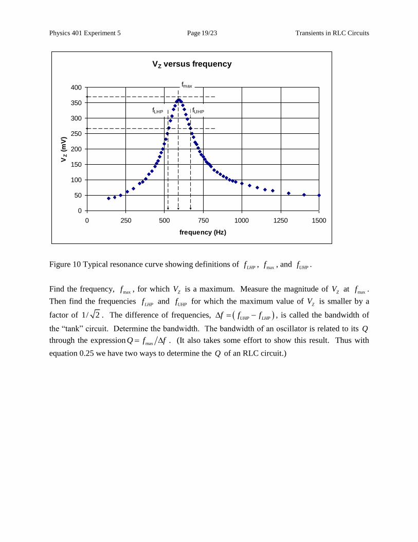
Physics 401 Experiment 5 Page Transients in RLC Circuits 19/23
VZ versus frequency
0
50
100
150
200
250
300
350
400
0 250 500 750 1000 1250 1500
frequency (Hz)
VZ (
mV
)
fUHPfLHP
fmax
Figure 10 Typical resonance curve showing definitions of LHP
f , max
f , and UHP
f .
Find the frequency, max
f , for which Z
V is a maximum. Measure the magnitude of Z
V at max
f .
Then find the frequencies LHP
f and UHP
f for which the maximum value of Z
V is smaller by a
factor of 1/ 2 . The difference of frequencies, UHP LHPf f f , is called the bandwidth of
the “tank” circuit. Determine the bandwidth. The bandwidth of an oscillator is related to its Q
through the expressionmax
Q f f . (It also takes some effort to show this result. Thus with
equation 0.25 we have two ways to determine the Q of an RLC circuit.)
Physics 401 Experiment 5 Page Transients in RLC Circuits 20/23
V. Report
The report consists of data, plots, and discussion from the different parts of the laboratory.
1. From part IV A above plot of 21/T versus 1/ C . Show from your data that neglect of the
2
2R L term in Equation (0.20) is justified. Then plot 2T versus C . Use the LINEST
function of Excel to determine the slope and the error in the slope of this line.
2. From part 2 IV B above plot the logarithmic decrement, , versus B
R . Determine the
extra “series” resistance needed to account for the negative intercept of this plot.
Compare the extra resistance to the resistance of the winding and the parallel
combination of the coupling resistor and input impedance of the Wavetek™.
3. From part IV C above use Excel to plot 2
criticalR versus 1/ C from your data. Also make
a plot of the prediction for 2
criticalR versus 1/ C using Equation (0.29). Comment on
agreement or disagreement between your data and the prediction.
4. From part IV D use Excel to plot the voltage across the capacitor versus frequency. On
the same graph, plot Equation (0.34), the magnitude of the impedance versus frequency.
Determine the resonant frequency, max
f , and bandwidth, f from your data. Make a
comparison between the theoretical expression and your experimental results.
5. In general discuss agreement and discrepancies of your measurements with expectations,
and suggest possible improvements to the laboratory exercise.
Physics 401 Experiment 5 Page Transients in RLC Circuits 21/23
Appendix I
Derivation of series RLC equation.
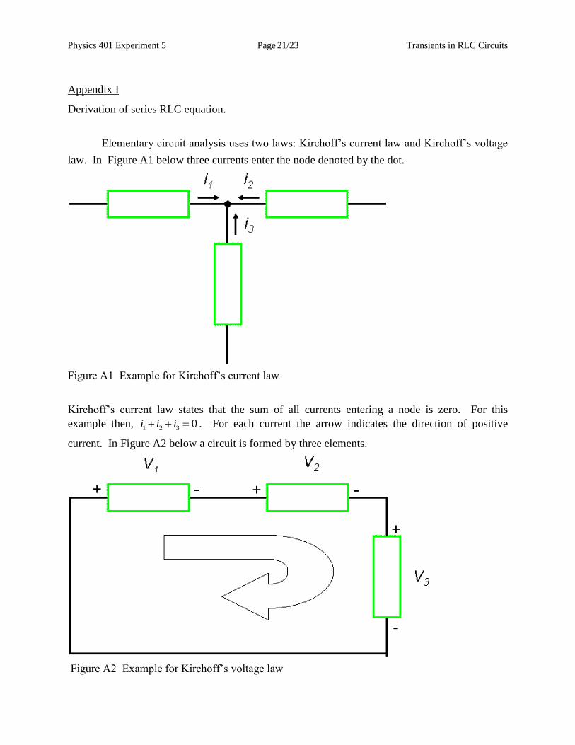
Elementary circuit analysis uses two laws: Kirchoff’s current law and Kirchoff’s voltage
law. In Figure A1 below three currents enter the node denoted by the dot.
Figure A1 Example for Kirchoff’s current law
Kirchoff’s current law states that the sum of all currents entering a node is zero. For this
example then, 1 2 3 0i i i . For each current the arrow indicates the direction of positive
current. In Figure A2 below a circuit is formed by three elements.
Figure A2 Example for Kirchoff’s voltage law
Physics 401 Experiment 5 Page Transients in RLC Circuits 22/23
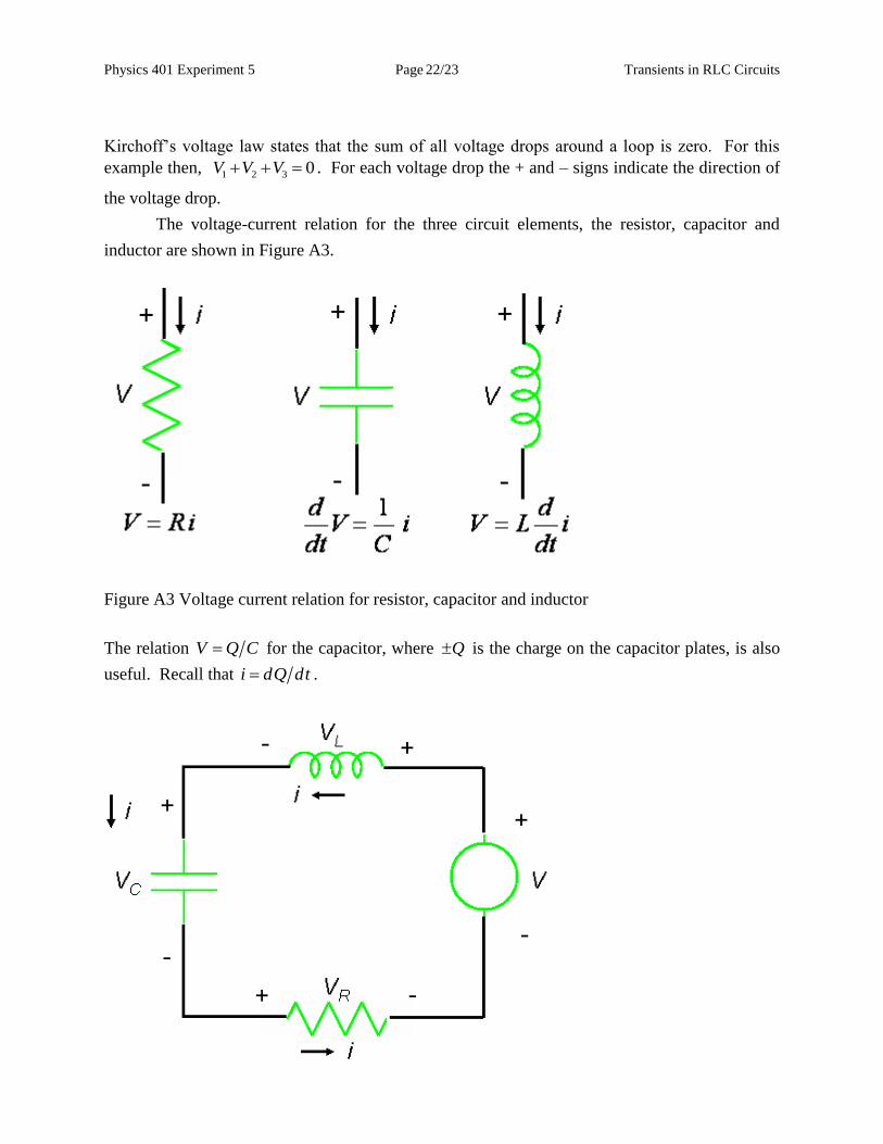
Kirchoff’s voltage law states that the sum of all voltage drops around a loop is zero. For this
example then, 1 2 3 0V V V . For each voltage drop the + and – signs indicate the direction of
the voltage drop.
The voltage-current relation for the three circuit elements, the resistor, capacitor and
inductor are shown in Figure A3.
Figure A3 Voltage current relation for resistor, capacitor and inductor
The relation V Q C for the capacitor, where Q is the charge on the capacitor plates, is also
useful. Recall that i dQ dt .
Physics 401 Experiment 5 Page Transients in RLC Circuits 23/23
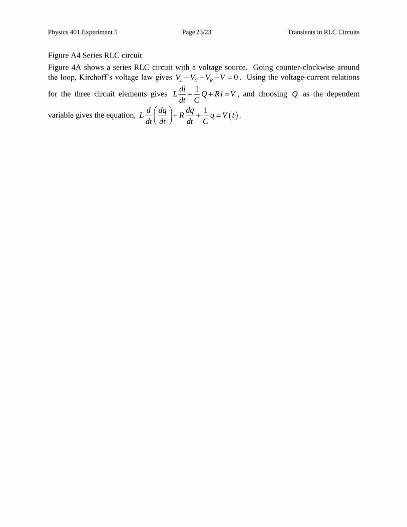
Figure A4 Series RLC circuit
Figure 4A shows a series RLC circuit with a voltage source. Going counter-clockwise around
the loop, Kirchoff’s voltage law gives 0L C RV V V V . Using the voltage-current relations
for the three circuit elements gives 1di
L Q Ri Vdt C , and choosing Q as the dependent
variable gives the equation, 1d dq dq
L R q V tdt dt dt C
.