university of florida thesis or dissertation formatting
TRANSCRIPT

1
ENHANCED CONTROL PERFORMANCE AND APPLICATION TO FUEL CELL SYSTEMS
By
VIKRAM SHISHODIA
A DISSERTATION PRESENTED TO THE GRADUATE SCHOOL OF THE UNIVERSITY OF FLORIDA IN PARTIAL FULFILLMENT
OF THE REQUIREMENTS FOR THE DEGREE OF DOCTOR OF PHILOSOPHY
UNIVERSITY OF FLORIDA
2008

2
© 2008 Vikram Shishodia

3
To Carmen

4
ACKNOWLEDGMENTS
I would like to express my deepest gratitude to my advisor Dr. O. Crisalle for his support
and guidance without which this work would not have been possible. I thank the members of my
supervisory committee, Dr. H. Latchman, Dr. G. Hoflund, Dr. W. Lear, and Dr. S. Svoronos, for
their guidance and serving on my supervisory committee.
I thank my colleagues in the research group who provided insightful conversations on my
research topics, besides being great friends. I would especially like to thank Christopher Peek
for providing the sample code for ramp tracking which expedited the progress on the problem
significantly. I also thank him for all the insightful discussions. I thank my parents for their
love, support and encouragement that they have given me throughout my life and during the
completion of this work.
I would like to express my deepest gratitude to my spiritual teacher Gurumayi
Chidvilasananda who has been there for me during every step of my life. Finally, I wish to thank
my wife and kids, who have been very supportive, loving and understanding during this journey.

5
TABLE OF CONTENTS page
ACKNOWLEDGMENTS ...............................................................................................................4
LIST OF TABLES...........................................................................................................................7
LIST OF FIGURES .........................................................................................................................8
ABSTRACT...................................................................................................................................11
CHAPTER
1 INTRODUCTION ..................................................................................................................13
2 VIRTUAL CONTROL LABORATORY...............................................................................15
2.1 Introduction...................................................................................................................15 2.2 Objective .......................................................................................................................17 2.3 Inverted Pendulum ........................................................................................................17 2.4 Control Design ..............................................................................................................20 2.5 Realization of an Inverted-Pendulum VCL ..................................................................25 2.6 Conclusions...................................................................................................................29
3 PI AND PI2 CONTROLLER TUNING FOR TRACKING THE SLOPE OF A RAMP.......38
3.1 Introduction and Background........................................................................................38 3.2 Problem Statement and Approach.................................................................................40 3.3 Results and Discussion..................................................................................................43
3.3.1 Tuning Parameters of Controllers .....................................................................43 3.3.2 Comparison of the Performance of the PI and PI2 Controllers .........................44 3.3.3 Comparison of Metrics......................................................................................46 3.3.4 Comparison of PI (ITAE) Controller with Literature Precedents.....................47 3.3.5 Local Minima versus Global Minima ...............................................................48
3.4 Conclusions...................................................................................................................48
4 GENERALIZED PREDICTIVE CONTROL FOR FUEL CELLS .......................................61
4.1 Introduction...................................................................................................................61 4.2 Fuel Cell System Background.......................................................................................61 4.3 Objectives of the Research............................................................................................64 4.4 Fuel Cell Model ............................................................................................................64 4.5 Literature Precedents fo Fuel Cell Control Designs .....................................................66
4.5.2 Feedforward Strategy........................................................................................67 4.5.2.1 Static feedforward controller ..............................................................67 4.5.2.2 Dynamic feedforward controller.........................................................68

6
4.5.3 Combination of Static Feedforward with Optimal Feedback Controllers ........69 4.5.3.1 Case where the performance variable is measurable ..........................69 4.5.3.2 Case where the performance variable is not measurable....................71
4.6 Generalized Predictive Control .....................................................................................72 4.7 Battery of Observers .....................................................................................................79 4.8 Simulation Studies and Results.....................................................................................81
4.8.1 Generalized Predictive Control Results ............................................................82 4.8.1.1 Case where the performance variable is measured.............................82 4.8.1.2 Performance variable not measured....................................................83
4.8.2 The GPC Approach Evaluated for Robustness .................................................85 4.8.2.1 Case where the performance variable is measured.............................86 4.8.2.2 Case where the performance variable is not measured.......................86
4.8.3 Comparison of the GPC Strategy with Prior Control Designs..........................88 4.8.3.1 Case where all states are measured-sFF with LQR feedback control 88 4.8.3.2 Case where all states are not measured-observer design ....................89 4.8.3.3 Comparison of controller performance with respect to robustness ....90
4.8.4 Feedforward Control Designs ...........................................................................92 4.8.4.1 Case of original model........................................................................92 4.8.4.2 Case of model uncertainty ..................................................................94
4.9 Conclusions...................................................................................................................95
5 CONCLUSIONS AND PROPOSITIONS FOR FUTURE WORK.....................................132
5.1 Conclusions.................................................................................................................132 5.2 Future Work ................................................................................................................133
APPENDIX
A OFFSET BETWEEN AUXILLIARY AND ORIGINAL RAMP........................................134
B OBSERVER DESIGN USING TRANSFER FUNCTION..................................................136
LIST OF REFERENCES.............................................................................................................137
BIOGRAPHICAL SKETCH .......................................................................................................140

7
LIST OF TABLES
Table page 3-1 The PI2 controllers optimized tuning parameters linear least square fit equations............52
3-2 The PI controllers optimized tuning parameters linear least square fit equations. ............53
3-3 Values of the plant parameters used compare the performance of the controllers. ...........53

8
LIST OF FIGURES
Figure page 2-1 Inverted pendulum. ............................................................................................................31
2-2a Front panel of the VCL where all states are measured. .....................................................32
2-2b Front panel of the VCL showing observer.........................................................................33
2-3 Interaction panel of inverted pendulum VCL. ...................................................................34
2-4 Controller tab of the navigation panel. ..............................................................................35
2-5 Analysis tab of the navigation panel. .................................................................................36
2-6 Simulation tab of the navigation panel. .............................................................................37
3-1 Ramp r and auxiliary ramp ra with constant slope, α. .......................................................49
3-2 Closed loop transfer function representation of plant and controller. ...............................49
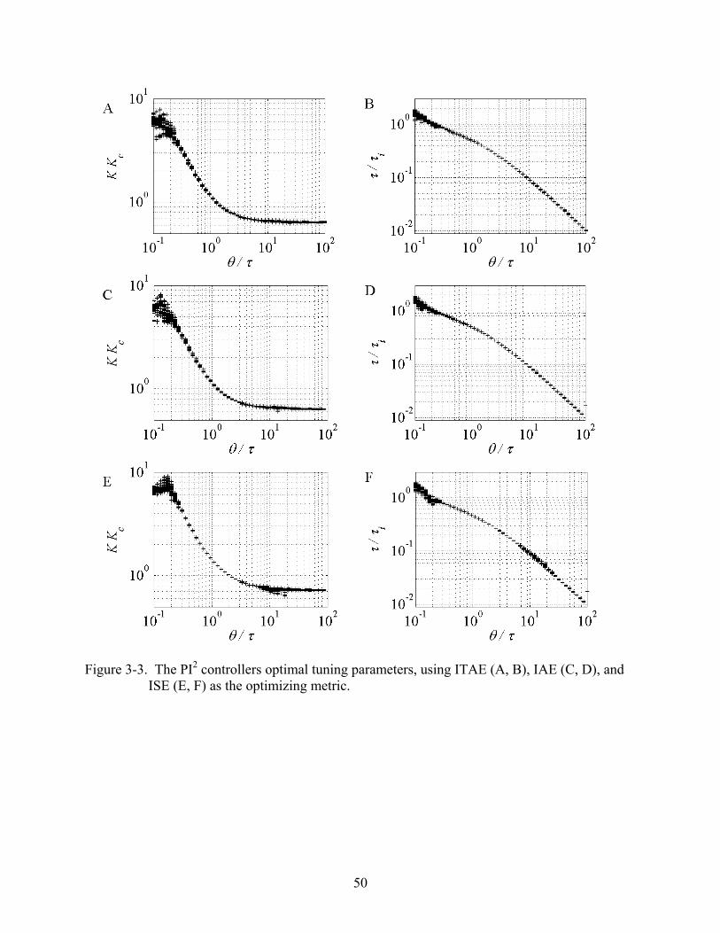
3-3 The PI2 controllers optimal tuning parameters, using ITAE (A, B), IAE (C, D), and ISE (E, F) as the optimizing metric. ..................................................................................50
3-4 The PI controllers optimal tuning parameters, using ITAE (A, B), IAE (C, D), and ISE (E, F) as the optimizing metric. ..................................................................................51
3-5 The PI2 and PI controllers’ ramp tracking and slope tracking performance using the optimal ITAE control parameters. .....................................................................................54
3-6 The PI2 and PI controllers’ ramp tracking and slope tracking performance using the optimal IAE control parameters.........................................................................................55
3-7 The PI2 and PI controllers’ ramp tracking and slope tracking performance using the optimal ISE control parameters. ........................................................................................56
3-8 The ITAE, IAE, and ISE metrics comparison for three plants, using the PI controllers A), B), and C).....................................................................................................................57
3-9 The ITAE, IAE, and ISE metrics comparison for three plants, using the PI2 controllers A), B), and C). .................................................................................................58
3-10 The PI controllers tuned using the ITAE metric compared with Belanger and Luyben and Peek’s controllers for three plants A), B), and C).......................................................59
3-11 Contour plots for the PI controller tuned using the ITAE metric for the three plants A), B), and C).....................................................................................................................60

9
4-1 Schematic of fuel cell system. ...........................................................................................96
4-2a Fuel cell system showing input u, disturbance w, and outputs z1, z2, y1, y2, y3...................97
4-2b Fuel cell system showing sFF with feedback controller....................................................98
4-3 Matrices defining the LTI model for the fuel cell model excluding sFF...........................99
4-4 Matrices defining the LTI model for the fuel cell including sFF. .....................................99
4-5 The sFF control configurations for fuel cell system. .......................................................100
4-6 The dFF controller: (a)Schematic diagram, and (b)transfer function representation. .....101
4-7 The sFF schematic with feedback controller. ..................................................................102
4-8 The GPC design in feedback block diagram....................................................................103
4-9 Disturbance profile used for simulation purposes. ..........................................................104
4-10 The GPC control strategy implementation on the nonlinear fuel cell model in the case when the controlled variable is measured. ...............................................................105
4-11 The GPC feedback with four observers control scheme implementation on the nonlinear fuel cell model. ................................................................................................106
4-12 The Norm of errors from the battery of observers...........................................................107
4-13 The switching pattern of the battery of observers............................................................108
4-14 Final voltage to the compressor. ......................................................................................109
4-15 Observer 1, error between measured and estimated values. ............................................110
4-16 Observer 2, error between measured and estimated values. ............................................111
4-17 Observer 3, error between measured and estimated values. ............................................112
4-18 Observer 4, error between measured and estimated values. ............................................113
4-19 The GPC feedback with three observers control scheme implementation on the nonlinear fuel cell model. ................................................................................................114
4-20 The GPC feedback with two observers control scheme implementation on the nonlinear fuel cell model. ................................................................................................115
4-21 The GPC feedback with one observer control scheme implementation on the nonlinear fuel cell model. ................................................................................................116

10
4-22 The GPC control strategy implementation on the nonlinear fuel cell model with a parameter changed from the value used for control design. ............................................117
4-23 The GPC controller with the LQG observer control strategy implementation on the altered nonlinear fuel cell model......................................................................................118
4-24 The GPC controller with the 4 observers control strategy implementation on the altered nonlinear fuel cell model......................................................................................119
4-25 Comparison of the GPC control strategy with the sFF controller combined with LQR feedback strategy on the unaltered nonlinear fuel cell model when the performance variable is measurable......................................................................................................120
4-26 The sFF with the LQG observer and LQR feedback, compared to GPC with the LQG Observer control strategy implementation on the unaltered nonlinear fuel cell model when the performance variable is not measurable. ..........................................................121
4-27 The sFF with the LQG observer and LQR feedback, compared to GPC with the 4 observers control strategy implementation on the unaltered nonlinear fuel cell model when the performance variable is not measurable. ..........................................................122
4-28 The sFF with the LQR feedback, compared to GPC, when performance variable is measurable on the altered nonlinear fuel cell model. ......................................................123
4-29 The sFF with the LQG observer and the LQR feedback compared to the GPC with the LQG observer control strategy on the altered nonlinear fuel cell model...................124
4-30 The sFF with the LQG observer and the LQR feedback compared to the GPC with the 4 observers control strategy on the altered nonlinear fuel cell model. ......................125
4-31 The sFF and dFF strategies and the GPC control strategy, performance compared when applied on the unaltered nonlinear fuel cell model. ...............................................126
4-32 The sFF and dFF strategies and the GPC control strategy with the LQG observer, performance compared when applied on the unaltered nonlinear fuel cell model. .........127
4-33 The performances of the sFF and dFF strategies and the GPC with the 4 observers control strategy compared when applied on the unaltered nonlinear fuel cell model. ....128
4-34 The sFF and dFF strategies and the GPC control strategy, performance compared when applied on the altered nonlinear fuel cell model. ...................................................129
4-35 The sFF and dFF strategies and the GPC control strategy with the LQG observer, performance compared when applied on the altered nonlinear fuel cell model. .............130
4-36 The performance of sFF and dFF strategies and the GPC with 4 observers control strategy compared when applied on the altered nonlinear fuel cell model......................131

11
Abstract of Dissertation Presented to the Graduate School of the University of Florida in Partial Fulfillment of the Requirements for the Degree of Doctor of Philosophy
ENHANCED CONTROL PERFORMANCE AND
APPLICATION TO FUEL CELL SYSTEMS
By
Vikram Shishodia
May 2008
Chair: Oscar D. Crisalle Major: Chemical Engineering
The inverted-pendulum virtual control lab, a simulation environment for teaching
advanced concepts of process control, is designed using the LabVIEW software tool. Significant
advantages of using this simulation tool for pedagogical purposes include avoiding the potential
issue of schedule conflicts for securing equipment-access time in a physical laboratory and
providing a learning resource that becomes accessible to students located in remote geographical
places.
A set of tuning relationships are proposed for standard proportional-integral controllers and
proportional double-integral controllers for the purpose of tracking the slope of a ramp trajectory.
Three different performance metrics are investigated to serve as the criteria for optimality, and a
numerical optimization procedure is used to minimize each metric over 20,000 different plants.
The proportional integral controller with tuning parameters selected to optimize value of the
integral of the time-weighted absolute error is recommended for tracking the slope of a ramp
trajectory.
A generalized predictive control (GPC) strategy is proposed for a fuel cell system, where
the controller incorporates a measured disturbance in the control design. The control objective is
to maintain oxygen excess ratio at a prescribed constant value. The performance of the GPC

12
control design is compared with that of the controllers proposed in literature for various
scenarios including model uncertainty. The GPC controller has zero offset when the
performance variable is measured and performs better than competing designs offered in the
literature. The GPC controller is also robust with respect to model uncertainty. A battery of
observers with a switching strategy is proposed for estimating the value of the performance
variable when it is not measured. The GPC controller with a battery of observers has no offset
demonstrating better performance than analogous designs proposed in literature. However, the
control performance is not robust when the estimator battery is used and linear models used for
observer design are uncertain given that the response offset is not completely eliminated.

13
CHAPTER 1 INTRODUCTION
Issues relevant and critical to process control are discussed in this study. Chapter 2
investigates the design and implementation of a virtual control lab (VCL) for “The Inverted
Pendulum” problem. The LabVIEW software is used as the platform for simulating the Inverted
Pendulum model. The objective is to have a visual computer based application by virtue of
which advanced control concepts can be shared and taught to the audience who are primarily
students studying control theory and its applications. The VCL is designed in a manner such that
various scenarios for the implementation of the controllers can be achieved. The user is given
the choice of operating the application with the system in open-loop or closed-loop
configuration. The controller can be tuned manually by the user or use the tuned control
parameters computed by the specific control algorithm. The user is allowed to alter the values of
the poles for the closed loop system and see its visual impact by simulation performed by the
VCL. The VCL provides the opportunity to be operated in the scenarios when all the controlled
variables are measurable and also when all of them are not measurable. In the case when the
performance variables are not measurable an observer is incorporated in the control design to
estimate their value. The impact of all the changes performed in the VCL are displayed visually
by the animation of the inverted pendulum system. This key feature of the VCL allows the user
to see the visual impact of changing different components of control system and hence
facilitating the process of learning.
Chapter 3 discusses the problem of controller design tuning for tracking the slope of a
ramp. The control objective is to place the output of the system in a linear zone parallel to a
ramp trajectory. A first order system with time delay is considered for this study. Two kinds of
controllers are used for this study namely, proportional-integral and proportional double-integral.

14
Both the controllers serve the purpose of positioning the system in the desired linear zone which
is parallel to a given ramp profile. There is an offset with respect to the ramp observed when
only one integrator is used. Zero offset with the ramp is observed when two integrators are used
in the controller. In both cases , the control objective is met which is to track the slope of the
ramp trajectory.. Three different metric are employed to evaluate the performance of the
controllers. The MATLAB platform in conjunction with SIMULINK module is used for
acquiring the optimized controller parameters.
Chapter 4 discusses a generalized predictive control (GPC) strategy proposed for a fuel cell
system. The control objective is to regulate the value of the performance variable i.e., the
oxygen excess ratio at a desired value. The performance of the GPC control design is compared
with that of controllers proposed in prior literature. Various scenarios are considered, including
the cases of model uncertainty and unmeasured performance variable. The GPC controller
exhibits zero offset in all cases when the performance variable is measured, and also ensure zero
or negligible offset when the performance variable is estimated via a battery of estimators.

15
CHAPTER 2 VIRTUAL CONTROL LABORATORY
2.1 Introduction
There is a need for the development of internet-based non-conventional pedagogical tools
for delivering knowledge to students on various topics of study. The drive stems from the
various advantages that these environments offer. First, these applications do not depend on the
availability of a physical setup or facility to run experiments [1, 2]. They are also not limited in
terms of the number of users who can access the application at any given time, as long as
appropriate adjustments are done in the server side of application. There is also no adverse safety
issue or concern of damaging expensive equipment when the product is not used correctly. Less
training is required for the user to be able to run the tool. Compared to a traditional physical
laboratory setup, in these virtual environments, there is more of an opportunity to be able to
realize a physical system and introduce more advanced topics and see their effects on the system.
A software application that simulates the behavior of a physical system, provides animation to
depict how the system behaves, and provides an interface so that the user can observe changes
made on the system performance, is highly beneficial from a learning and educational
standpoint. The application is referred to as a virtual laboratories since the nature of the “Lab” or
the application is “virtual” as it is a software emulator of the physical plant and can be
potentially used to remotely control actual physical equipment via web and networking [1, 3-6].
From the perspective of enhancing the learning experience, the virtual control lab (VCL)
supports learning by all three modes, namely active, flexible, and discovery learning. In active
learning, tools and material are made available to students so that they can use these resources to
actively learn and reinforce the theoretical concepts. Traditionally, physical laboratories,
equipment and experimental apparatus are provided to students to reinforce and test the

16
understanding of the student’s comprehension of the theory. With limitation of available
resources and costs associated with the overall management of logistics, at times this can be a
challenging task, which can prove to be not only quite expensive, but also involve safety issues.
In those circumstances the VCL can be an excellent solution. It doesn’t necessarily need to be a
complete replacement, but it can be used in conjunction with existing physical setups to promote
active learning.
Flexible learning provides opportunities to learn class material when the students or
instructor might be having challenges in terms of establishing meeting times, scheduling or
location [7]. For instance, if an individual is a part-time student with the obligations of a full-
time student, that person might have challenges meeting lab times scheduled during regular work
hours. The VCL is a most valuable tool to accommodate those circumstances. From the comfort
of home and in a more appropriate time, that individual can complete the exercises/material if the
VCL is utilized. The VCL is flexible with respect to the schedule and logistics limitations of an
individual.
The VCL also supports learning via discovery mode. In this scenario, an environment is
provided where the student has minimal supervision or instruction [8]. The student is
encouraged to learn by making changes and observing the impact of these changes. There are
some significant challenges in implementing such a setup in the alternative scenario of a physical
laboratory. Due to safety and cost considerations, facilities that promote discovery learning are
few. A VCL designed for the purpose, again, proves to be an excellent resource to implement
safe and cost-effective learning via discovery.
There are various implementations of virtual and remote labs reported in the literature.
There are several World Wide Web based labs which foster learning by different modes [3, 9-

17
11]. Most of these virtual labs, however, have a few shortcomings in terms of their usage. Many
do not provide a sufficiently high level of interactivity with the user. Significant modifications
need to be made to the program to implement any changes. Another disadvantage that most of
the current virtual labs have is that they are developed on a proprietary software platform. At
times significant familiarity with that software is needed to be able to utilize the application.
2.2 Objective
The intent is to build a VCL module that treats some advanced-level control concepts and
serves as a pedagogical tool that overcomes shortcomings that existing virtual labs pose from a
learning perspective and user interface. The infrastructure created by Peek et al. is used for
implementing an Inverted Pendulum VCL [12]. The intent is to develop an animated control
module that reinforces advanced control concepts with a friendly user interface. Some examples
of key control concepts illustrated in the VCL are linear state-space modeling, controllability,
pole placement and observability analysis. Sections 2.3 and 2.4 discuss the Inverted Pendulum
system, its dynamics and the associated control concepts. Section 2.5 describes the
implementation of the Inverted Pendulum system as a VCL using the LabVIEW software and its
animation features [13]. Finally, conclusions from this effort are summarized in Section 2.6.
2.3 Inverted Pendulum
The inverted pendulum considered consists of a spherical bob attached to a cart by a rod.
A schematic diagram is given in Figure 2.1. The mass of the rod is assumed to be negligible.
The rod is mounted by a hinge at the center of the cart. The input of the system is a horizontal
force applied to the cart. The cart is free to move only along one coordinate which is the
horizontal z-axis. The pendulum is free to rotate 360 degrees with respect to the cart in the x-z
plane where the x-axis is vertical. It is assumed that there is no friction between the pendulum
and the cart at the hinge.

18
The goal is to keep the pendulum in an upright position by manipulating the value of the
applied force. The system is inherently nonlinear. To apply linear control theory, the dynamics
must be linearized, and represented as a standard state-space realization. Consequently, the
system is linearized for small values of the angle that the pendulum makes with the vertical.
The nonlinear equations describing the dynamics of the system are
⎟⎠⎞
⎜⎝⎛ −+
+= θθθ
θcossinsin
sin
1 z 2
2gθl
mf
mM
(2-1)
and ⎟⎠⎞
⎜⎝⎛ +
+−−⎟⎠⎞
⎜⎝⎛ +
= θθθθθθ
θ sinsincoscossin
1 2
2
gm
Mmlmf
mMl
(2-2)
where dz/dt z = (2-3a)
and /dtd θθ = (2-3b)
where M is the mass of the cart, m is the mass of the pendulum bob, l is the length of the
pendulum rod, g is the acceleration due to gravity, z is the horizontal position of the cart, θ is the
angle that the pendulum makes with the vertical, and f is the force (control input) acting on the
cart [14].
A linear state-space system is derived from Eqs. 2-1 – 2-3 by linearizing about an
operating point ( ),,,, fzz θθ , where
0=z (2-4)
0=z (2-5)
0=θ (2-6)
0=θ (2-7)
0=f (2-8)

19
The deviation variables for the linear state-space model are
zzx −=1 (2-9)
zzx −=2 (2-10)
θθ −=3x (2-11)
θθ −=4x (2-12)
ffu −= (2-13)
After linearization about the point
)0,0,0,0,0(),,,,( =fzz θθ (2-14)
the resulting standard linear state-space model
ubAxx += (2-15)
is given by the equation
u
Ml
M
MlM)g(m
Mmg
⎥⎥⎥⎥⎥⎥⎥⎥
⎦
⎤
⎢⎢⎢⎢⎢⎢⎢⎢
⎣
⎡
−
+
⎥⎥⎥⎥⎥⎥⎥⎥
⎦
⎤
⎢⎢⎢⎢⎢⎢⎢⎢
⎣
⎡
+
−
=
1
0
1
0
000
1000
000
0010
xx (2-16)
where the elements of the state vector x are distance (x1 = z), velocity (x2 = z ), angle (x3 = θ),
and angular velocity (x4 = θ ), and where
⎥⎥⎥⎥⎥⎥⎥⎥
⎦
⎤
⎢⎢⎢⎢⎢⎢⎢⎢
⎣
⎡
+
−
=
0)(00
1000
000
0010
MlgMm
Mmg
A (2-17)

20
⎥⎥⎥⎥⎥⎥⎥⎥
⎦
⎤
⎢⎢⎢⎢⎢⎢⎢⎢
⎣
⎡
−
=
Ml
M
1
0
1
0
b (2-18)
The control is u, which is the force acting on the cart. The standard output model
xCy = (2-19)
relates the output y to matrix C and state vector x, where the output matrix C is the identity
matrix
⎥⎥⎥⎥
⎦
⎤
⎢⎢⎢⎢
⎣
⎡
=
1000010000100001
C (2-20a)
in the case where all four states are measured. For the case where only one state is measurable,
the output matrix C adopts a row-vector form of all zeros, except for one entry that is unity at the
location corresponding to the measured state. For the particular case where the state x1, namely
the distance of the cart from its original horizontal position, is the only measured state, the output
matrix C adopts the form
[ ]0001=C (2-20b)
2.4 Control Design
When the system is in the unforced configuration, a stability check done by calculating the
eigenvalues of matrix A reveals that there is one eigenvalue that lies in the open right half plane,
implying that the system in its unforced state is unstable.

21
This is a regulation problem, as the objective is to make the states evolve towards zero
value. For the implementation of the controller, a test for controllability needs to be performed
to verify that the system is indeed controllable. The requirement for controllability is that
0Qc ≠)det( (2-21)
where [ ]bAbAAbbQ 32c = (2-22)
Using the definitions for A given in Eq. 2-5 and for b given in Eq. 2-6, it follows that
⎥⎥⎥⎥⎥⎥⎥⎥
⎦
⎤
⎢⎢⎢⎢⎢⎢⎢⎢
⎣
⎡
−=
0
1
0
1
Ml
M
Ab ,
⎥⎥⎥⎥⎥⎥⎥⎥
⎦
⎤
⎢⎢⎢⎢⎢⎢⎢⎢
⎣
⎡
+−
=
22
22
)(
0
0
lMgMm
lMmg
bA ,
⎥⎥⎥⎥⎥⎥⎥⎥⎥
⎦
⎤
⎢⎢⎢⎢⎢⎢⎢⎢⎢
⎣
⎡
+−=
0
)(
0
22
22
3
lMgMm
lMmg
bA (2-23)
Hence,
⎥⎥⎥⎥⎥⎥⎥⎥
⎦
⎤
⎢⎢⎢⎢⎢⎢⎢⎢
⎣
⎡
+−−
+−−=
0)(01
)(010
001
010
22
22
2
22
lMgMm
Ml
lMgMm
Ml
lMmg
M
lMmg
M
cQ (2-24)
Obviously matrix cQ in Eq. 2-11 is of full rank, thus
0)det( ≠cQ (2-25)
which implies that the system Eq. 2-4 is indeed controllable. The analysis of controllability
presented here is found in standard references [32-34].
Two scenarios are considered:
1. All states are measured.
2. Some states are not measured.

22
In the case of the first scenario in which all states are measured, a full-state feedback
approach is used in the form of the proportional state feedback control law
Fx−=u (2-26)
where F is a proportional gain used to address the regulation problem.
To determine an appropriate value for matrix F, first substitute the value of u given by Eq.
(2-26) into the state space equation Eq. (2-15) leading to
)( FxbAxx −+= (2-27)
The standard solution to Eq. 2-14 is given by the Variation of Parameters formula as
te )(0
BFAxx −= (2-28)
where 0x is the vector of the initial value of the state vector x [36]. Ackerman’s pole placement
algorithm is employed for computing the value of the matrix F that places the poles of the A-BF
system in the desired location [36].
In the case of the second scenario, in which all states of the system are not measurabed, a
Luenberger Observer is incorporated in the controller to estimate the value of the states. Before
carrying out an observer design, a check is performed to verify if the system is observable when
only one state is measured. The first state, the distance of the cart from the original position, is
the only state that is assumed to be measurable. For the system to be observable, the condition
0)det( ≠oQ (2-29)
should be satisfied, where the observability matrix oQ is given by
⎥⎥⎥⎥⎥
⎦
⎤
⎢⎢⎢⎢⎢
⎣
⎡
=
3
2
CACACAC
Q o (2-30)
Matrix A is defined by Eq. (2-17) and matrix C by Eq. 2-20b. The expressions

23
[ ]0010=CA (2-31)
⎥⎦⎤
⎢⎣⎡ −
= 0002
MmgCA (2-32)
and ⎥⎦⎤
⎢⎣⎡ −
=Mmg0003CA (2-33)
can be used to readily build the observability matrix oQ described by Eq. 2-17, yielding
⎥⎥⎥⎥⎥⎥⎥⎥
⎦
⎤
⎢⎢⎢⎢⎢⎢⎢⎢
⎣
⎡
−
−=
Mmg
Mmgo
000
000
0010
0001
Q (2-34)
Since matrix oQ is diagonal, its determinant is simply the product of the diagonal terms.
Hence,
( ) 0det 2
22
≠=M
gmoQ (2-35)
Given that the determinant is nonzero, it follows that oQ is of full rank, and therefore the
system is observable. The analysis of observability presented here is also found in standard
references [34-36].
The standard equations for observer design
ubAxx += (2-36)
)ˆ(ˆˆ yyLbxAx −++= u (2-37)
produce estimated states x and estimated outputs xCy ˆˆ = as a function of the measured system
output Cxy = , and the Luenberger gain L, in Eq. 2-37. The control input

24
xFˆ−=u (2-38)
is used to place the poles of Eq. 2-36 at the desired locations. The error
xxε ˆ−= (2-39)
is defined as the difference between the actual values of state vector x and estimated values of
state vector x . Hence, the derivative of the error
xxε ˆ−= (2-40)
is computed by differentiating Eq. 2-39. Substituting Eq. 2-36 and Eq. 2-37 in Eq. 2-40 yields
LC)ε(Aε −= (2-41)
Invoking now the Variation of Parameters formula the solution to the differential equation
Eq. 2-41 is
te )(0
LCAεε −= (2-42)
where )0(ˆ)0(0 xxε −= is the initial value of the error ε , )0(x is an initial guess of the value of
the estimated state vector, and )0(x is the initial value of the state vector .
The poles of matrix A-LC should lie on the open half plane for the value of error ε to
evolve to zero. The poles are placed at the desired location by an appropriate choice of L, which
for low-order systems as the one considered here can be easily done via Ackerman’s Pole
Placement algorithm.
Linear quadratic regulator control design. A Linear quadratic control regulator (LQR)
control design is implemented in the VCL. The LQR control law
Kx−=u (2-43)
is obtained by minimizing the cost function
dtuRuuuJ TTT )2()(0∫∞
++= NxxQx (2-44)

25
with respect to u . The weighting matrix Q must be symmetric positive semi-definite, and R
symmetric positive definite. The weighting function N is specified to be zero.
For a linear state space system
uBAxx += (2-45)
the solution to the minimization of the cost function results in the steady-state Riccatti equation
[36]
0Q)NS(BN)R(SBSASA TT1T =+++−+ − (2-46)
The acceptable solution to Eq. 2-46 is a positive definite matrix S which is then used to specify
K from the expression
)NS(BRK TT1 += − (2-47)
Since in this case 0=N , therefore
SBRK T1−= (2-48)
2.5 Realization of an Inverted-Pendulum VCL
The LabVIEW software and a VCL infrastructure proposed by Peek et al., is used for the
implementation of the Inverted Pendulum VCL [12, 13]. Previous software-based control-tools
for the inverted-pendulum system reported in the literature have significant value, but the VCL
developed in this study has a number of additional desirable pedagogical features [14]. Initially,
stand-alone VIs and subVIs are generated using LabVIEW software for different components of
the design before integrating them as a part of a monolithic VCL. There are several reasons why
National Instruments’ LabVIEW software is used for constructing the VCL. The ease of
structuring and maintaining a VCL is significantly high in this software. The LabVIEW
software has built-in features for deploying applications on the web. The software also has
toolkits specifically designed for control engineering. Implementation of a VCL using

26
LabVIEW does not rely on support from other software packages, as would be the case if some
higher-level language is used to implement the same features found in VCL.
Figure 2-2 shows the front panel of VCL as it appears to a student user. The key elements
are the Animation and Interaction Panels, respectively, located on the top and bottom-left areas
of the front panel. These two are very critical components of the VCL as the user makes most
modifications in the plant and controller setup in the Interaction panel and instantaneously
observes an animated result describing the plant and states in the Animation Panel. The
Animation Panel has a two-dimensional graphic representation of an inverted pendulum. When
the VCL is operated, the animated cart responds to the control input by moving to the left or
right and causing a pendulum swing. The third panel is the Navigation Panel on the bottom-right
area of the front panel. The Navigation Panel has five tabs (Information, Plant, Controller,
Analysis and Simulation), which provide various pieces of information about the VCL. More
information is given about these three panels in the ensuing subsections.
Animation, interaction and navigation panel. The animation panel plays the role of
providing a visual representation of the plant, namely an inverted pendulum. Any changes that
are made to the inverted pendulum mounted on the cart are visually depicted in the Animation
Panel.
The user has the ability to make changes to the plant and controller in the Interaction
Panel. The user can adjust plant parameters, initial condition of the states of the inverted
pendulum and assign the different values to control parameters to the controller of choice. The
user also has the ability to run the plant in Manual or in Auto mode. Figure 2-3 depicts some of
the various modes that the user can configure parameters in the Interaction Panel.

27
The user has to specify the initial states of the pendulum (position, velocity, angle of the
pendulum with the vertical and the angular velocity of the pendulum). The Animation Panel
constructs the visual representation of the inverted pendulum based on the information that the
user provides. The user has the flexibility of running the VCL in the following two scenarios:
(1) all states are measured, or (2) only one state is measured. Based on the choice of the user, an
implementation of the corresponding controller is given. When “Manual F” Control is in the
“Off” position, the user is allowed to choose the poles for the closed loop matrix A-BF and the
value of matrix F is calculated from Ackerman’s pole placement algorithm. The user can
immediately see the impact of poles chosen on the stability of the inverted pendulum in the
Navigation Panel under the Analysis tab. When the “Manual F” Control is in the“On” position,
the user has the ability to choose the values of the elements of matrix F. When the controller is
operated in “Luenberger Observer” mode, as shown in Figure 2-, the user has to provide the
desired poles for matrix A-LC. The only state that can be measured in this mode is the position
of the cart. When the controller is in “Off” mode, i.e., the system is in open loop configuration
with no feedback, the Analysis tab of the Navigation Panel shows that the pendulum is in an
unstable configuration, which is ascertained by the fact that there is one eigenvalue of the system
in the open right half plane. The Interaction and Animation panels provide a suite of options and
visual representation for the user.
The Navigation panel is located on the bottom-right area of the front panel of the VCL.
The Navigation panel has five tabs entitled: (1) Help, (2) Plant, (3) Controller, (4) Analysis, and
(5) Simulation. These tabs provide pertinent and critical information about the VCL to the user.
The Help tab, when clicked on, provides general information about the operation of the VCL.
The user can access the Help tab without having to leave the VCL. The Help tab displays an

28
embedded PDF file. The Plant and Controller tabs are also embedded PDF files which provide
information about the dynamics of the plant (inverted pendulum) and the controller (proportional
state feedback and Luenberger Observer). The nonlinear equations and linear state space system
for the inverted pendulum are explained in the Plant tab of the Navigation Panel. Figure 2-3
shows the Plant tab of the Navigation Panel. The Controller tab provides information about pole
placement and various other aspects of control design for inverted pendulum VCL, as shown in
Figure 2-4.
The Analysis tab, shown in Figure 2-5, has information about the tools and graphs that are
used in control theory. This tab has information about the transfer function, location of poles and
zeros in complex plane and Bode plot (frequency response). The Simulation tab, shown in
Figure 2-6, shows plots of the results of numerical simulations describing the states (position,
velocity, angle and angular velocity) and inputs as a function of time. Since this is a regulation
problem, when stable choices of eigenvalues are given, using the linear state space as the
dynamic model, all states converge to the value zero, regardless of the choice of initial state
vector. The Simulation tab provides the real time curves of all the states as a function of time.
The Runge-Kutta integration algorithm is employed to compute the numerical response of the
plant to the controlling input. When the controller is toggled between “On” and “Off” modes
(closed-loop and open-loop behavior, respectively) in the Interaction panel by the user, the
impact of that change on the value of states is depicted immediately in the Simulation tab.
The LQR control strategy, as shown in Figure 2-, employed in the VCL gives the user the
opportunity to implement different control choices, such as varying the weighting on different
elements of the cost function and displaying the corresponding LQR gain.

29
2.6 Conclusions
A VCL for the control of an Inverted Pendulum is described. The Inverted Pendulum is a
classic example of illustrating state-space model representations and demonstrating the classical
control concepts of controllability and observability. The animation features of the VCL provide
a visual description of how an inverted pendulum responds as a function of the input force
applied. The user is given the opportunity to run the VCL in different modes, such as in open-
loop and closed-loop configurations of the system.
The VCL can be utilized as a tool for enhancing learning. The three most widely
recognized learning modes (active learning, flexible learning, and learning via discovery) can be
easily executed using this VCL module. The module can be used in conjunction with a process
control lecture for demonstrating various concepts. The animation capabilities allows the user to
see the impact of every change that is made to the control configuration. The Analysis tab also
demonstrates that the open-loop configuration (unforced system) is unstable, as one of the
eigenvalues is in open right half plane. The user is given the choice of choosing the poles for the
system and noticing its impact on the plant. The user has the choice of running the VCL in two
modes: (1) all states measured or (2) only one state is measured and implementation of a
Luenberger Observer. This utilization of the VCL supports active learning of the control
material. The VCL can also be presented before or after a conventional lecture. In the first case,
the users’ motivation to learn about theory presented in class would be enhanced as they have the
opportunity to develop and experience with the VCL. In the later case, after the lecture is
delivered, an interaction with the VCL would serve as an excellent tool for reinforcing the
concepts taught in class. There is significant value in learning an abstract concept taught in
lecture and being able to relate to the concept by virtue of seeing the animation and graphs from

30
simulation. In an ideal scenario, the VCL should be used in all three modes (before, during, and
after lectures).
The tool can also be used to support group activities in a class for learning control theory
and doing control homeworks [15]. The modular feature of the VCL can be taken advantage of
by implementing sequential learning. In this mode, different versions of same VCL are
progressively given to the user as the class progresses. Each successive version makes more
features of the controller available to the user, hence helping students appreciate and learn faster
the concepts as they are progressively taught in the class.
To validate the benefits and effectiveness, it is proposed that the VCL should be used as a
pilot teaching tool in process control classes. The feedback obtained from the students would be
highly beneficial in optimizing and incorporating features that could enhance the learning
experience.

31
θ
mg
l
f
z
Mg
x
Figure 2-1. Inverted pendulum.

32
Figure 2-2a. Front panel of the VCL where all states are measured.

33
Figure 2-2b. Front panel of the VCL showing observer.

34
Figure 2-3. Interaction panel of inverted pendulum VCL.

35
Figure 2-4. Controller tab of the navigation panel.

36
Figure 2-5. Analysis tab of the navigation panel.

37
Figure 2-6. Simulation tab of the navigation panel.

38
CHAPTER 3 PI AND PI2 CONTROLLER TUNING FOR TRACKING THE SLOPE OF A RAMP
3.1 Introduction and Background
In certain applications tracking the slope of the ramp is more critical than tracking the
ramp itself. It is not unusual to encounter applications where the set point is the slope of a ramp
trajectory. For instance, while growing thin films on a substrate, it is desired that the
temperature of the substrate in the reactor increases at a steady rate (i.e., following a trajectory
with a specified slope). In these kinds of applications, it becomes crucial to adopt the
appropriate choice of controller type with effective values for the tuning parameters and an
appropriate metric to ensure adequate performance. Simplicity of tuning relationships plays a
critical role in the implementation of a controller. Most successful tuning relationships have
been developed via simulation [16, 17]. The cost function normally used involves the feedback
error, which is the difference between the set point and output of the plant.
A proportional-only controller leads to a steady state offset with respect to step changes in
set point. An integrator needs to be incorporated in the controller to eliminate the offset.
Similarly, for a ramp set point, a proportional-integral (PI) controller is not sufficient to remove
the steady state offset. In this case a controller with two integrators, that is a proportional
double-integral (PI2) controller, is needed to remove the offset [18]. However, a PI controller is
sufficient to track the slope of the ramp trajectory. Belanger and Luyben proposed a
proportional-integral-double integral controller relating the tuning parameters to the ultimate
gain and ultimate period of the plant [19]. Alvarez-Ramirez et al. extended the work of Belanger
and Luyben and coined the acronym PI2 [20]. Peek examined three different versions of PI2
controllers for tracking ramp set point [21].

39
This study investigates the problem of controller tuning for tracking the slope of a ramp
signal as depicted in Figure 3-1. The intent is to design a controller that leads the output
trajectory to follow a line parallel to the ramp. It is also critical to minimize transients. The
control performance is deemed as poor when the system experiences large deviations during the
transients.
To investigate the problem, a first order system with time delay is adopted as the plant
model. Since the set point is a ramp, integral action needs to be incorporated in the control
design. Two kinds of controllers are used for this study, namely a proportional-integral (PI)
controller and proportional double-integral (PI2) controller. Both controllers serve the purpose of
placing the system output on the desired line, parallel to the ramp set point. However, there is an
offset with respect to the original ramp trajectory when PI controllers are used because only one
integrator is included in the control scheme.
To identify the appropriate indicator to measure the performance of the controller with
respect to the system and objective in question, three different metrics are used: integral of the
time-weighted absolute error (ITAE), integral of the absolute error (IAE), and integral of the
square of error (ISE). Each of the controllers is tuned to minimize the metric value for a given
set of plant parameters. The Simplex optimization routine is used to acquire tuning parameters
via the minimization of the metric adopted. The MATLAB platform in conjunction with the
SIMULINK module is used for conducting the simulations. A set of optimal tuning relationships
for controllers to track the slope of a ramp for 20,000 different plants are presented. The
performance of all the controllers is evaluated and results are compared with the prior work of
Belanger and Luyben. The performance of the controllers is also compared with that of those
proposed by Peek.

40
3.2 Problem Statement and Approach
The objective is to use PI and PI2 controller to make a first-order plant with time delay
follow the slope of a ramp. The plant is represented by the transfer function
sp e
sKsG θ
τ−
+=
1)( (3-1)
where K is the gain, τ is the time constant, and θ is the time delay of the plant. The input to the
plant is denoted as u and the output as y. The transfer function representation of the PI controller
is
⎟⎟⎠
⎞⎜⎜⎝
⎛+=
sKsG
icc τ
11)( (3-2)
and the transfer function for the PI2 controller investigated here is
2
11)( ⎟⎟⎠
⎞⎜⎜⎝
⎛+=
sKsG
icc τ
(3-3)
where cK is the proportional gain, and iτ is the integral-action time constant. The plant and the
controller are configured in the closed-loop arrangement shown in Figure 3-2. The ramp
function serving as the set point in Figure 3-2 is given by
ttr α=)( (3-4)
where t is the time and the constant slope α is taken as 1=α .
Three error metrics are used for tuning the controllers, namely, the integral of the time-
weighted absolute error (ITAE), the integral of the absolute error (IAE), and the integral of the
square of error (ISE), respectively defined by the integral equations
∫ −=∞→
f
f
t
tdttytrtITAE
0
)()(lim (3-5)

41
∫ −=∞→
f
f
t
tdttytrIAE
0
)()(lim (3-6)
( )∫ −=∞→
f
f
t
tdttytrISE
0
2)()(lim (3-7)
where )(ty is the plant output and ft is the extent of time over which the metric is computed.
When the closed loop uses a PI controller, the output of the system exhibits a steady state
offset sse with respect to the original ramp characterized through the analytical expression
c
iss KK
eτ
= (3-8)
the derivation of which is given in the APPENDIX using Final Value Theorem. A modified or
auxiliary ramp )(tra is defined via the relationship
ssa etrtr −= )()( (3-9)
Figure 3-1 shows the ramp and the auxiliary ramp trajectories.
The corresponding auxiliary error metrics for PI controller, modified from Eq. 3-4, Eq. 3-5
and Eq. 3-6 are given by
∫ −=∞→
f
f
t
ata dttytrtITAE0
)()(lim (3-10)
∫ −=∞→
f
f
t
ata dttytrIAE0
)()(lim (3-11)
( )∫ −=∞→
f
f
t
ata dttytrISE0
2)()(lim (3-12)
where the aITAE is the auxiliary integral of the time-weighted absolute error, the aIAE is the
auxiliary integral of the absolute error, and the aISE is the integral of the square of error. It is to

42
be noted that in the case of PI2 controllers, the value of sse is zero i.e., )()( trtra = . Hence, the
ITAE, IAE and ISE error metrics for PI2 retain the original form of Eq. 3-5, Eq. 3-6, and Eq. 3-7,
respectively, even when all computations are carried out using their auxiliary counterparts.
The ITAE expression (Eq. 3-5) has been a popular choice for control parameter
optimization, as it assigns less weight to errors occurring in the initial times and more weight to
error at longer times. Error is defined as the closed-loop feedback difference between the
auxiliary set point and the output. This is traditionally a useful measure to adopt, as for a step
response it is inevitable that there is a relatively large error during initial times, which needs to
be given less significance compared to the error that is encountered at later times. The ITAE
may not be the best metric for the problem in question, however. The desired trajectory of the
output is the one which tracks the slope of the ramp without abrupt deviations in trajectory. The
ITAE is forgiving of aggressive output values at initial times as it gives less significance to error
at early times. Sometimes, it is desired to adopt a metric which gives an equal importance to
errors occurring at initial times as well. From that perspective, the two other metrics are also
used in this work for optimization purposes, namely, the IAE (Eq. 3-6) and the ISE (Eq. 3-7).
A routine in MATLAB is written to simulate the plant output for a given controller with its
parameters specified [22]. The simplex optimization routine is employed for tuning the control
parameters. For a fixed value of plant parameters (gain, time constant and time delay), the
parameters of the controller (proportional gain and integral action) are altered to minimize the
(ITAE, IAE or ISE) value of the cost function. For a PI controller, where there is offset with
respect to the ramp, an auxiliary ramp parallel to original one is constructed. The steady state
offset is calculated analytically using Eq. 3-8.

43
The three error metrics (ITAE, IAE and ISE) are minimized using the new ramp. These
metrics are defined over an infinitely long time; however, for practical purposes the final time is
chosen to be finite and defined by the formula
),max(15 θτ=ft (3-13)
The rationale behind this choice is that by this extent of final time, any reasonably performing
controller should make the value of error significantly small. The optimized tuning parameters
are non-dimensionalized by combining with plant parameters, and plots of optimized tuning
parameters were constructed. Time responses are constructed with the optimized values to verify
the responses of the process with the controlling action incorporated.
Peek analyzes the performance of three different configurations of PI2 controllers [21].
That study concludes that there is no significant difference in the performance of the three
configurations. The transfer function for PI2 controller given in Eq. 3-2 is used in this study as it
is the easiest to tune because it involves only two parameters, namely the proportional gain cK
and the integral-action time constant iτ .
3.3 Results and Discussion
3.3.1 Tuning Parameters of Controllers
Tuning parameters are calculated for both controllers PI and PI2 using the ITAE, IAE, and
ISE as the optimizing metric. The optimized controller parameters are nondimesionalised using
the plant gain and time constant [17]. The resulting plots of KKc versus θ/τ, and τ/τI versus θ/τ
are shown in Figures 3-3 and 3-4 for the PI2 and PI controllers. The tuning parameters obtained
using ITAE, IAE and ISE as the metric are shown in the first, second, and third row of each
figure, respectively. The plant parameters K, θ, and τ are selected such that K and τ range from
0.1 to 50. Twenty logarithmically equally-spaced points are considered for both K and τ in their

44
specified ranges. After each time constant τ is defined, the values of the delay parameter θ is set
by defining the ratio of θ/τ to range from 0.1 to 100, with 50 logarithmically equally-spaced
points inside the range. For a fixed value of θ/τ ratio, the value of θ is computed from the value
of τ and of the fixed θ/τ ratio. Hence, tuning parameters were obtained for 20,000 different
plants for each controller and for each metric.
The graphs in Figures 3-3 and 3-4 show that, in general, as the θ/τ ratio increases, the value
of the optimal KKc product and of the τ/τi ratio decrease. The value of the KKc product
represents the proportional control action on the closed loop system, and it is expected to vary
inversely to the θ/τ ratio. In other words, the control action will be higher for smaller values of
θ/τ ratio, and smaller as θ/τ increases. This is qualitatively reflected in Figures 3-3 and 3-4 for all
three optimizing metrics and for the two controllers considered. On the same vein, the τ/τi ratio
is indicative of integral action for the system and it is expected to behave analogously to the
proportional control action. The integral action should be more aggressive for smaller values of
θ/τ ratio compared to higher values of the ratio. This is, indeed, observed from Figures 3-3 and
3-4.
Least-square fits for the optimized control parameters are given in Tables 3-1 and 3-2 for
the PI2 and PI controller, respectively. The least square fit relates the optimal KKc product with
the θ/τ ratios and the optimal τ/τi ratio with the θ/τ ratio. If the KKc versus θ/τ curve and/or τ/τi
versus θ/τ curve is significantly nonlinear, a break point at a certain value of θ/τ ratio is identified
and two least-square fits are presented for the same curve, one above and one below the θ/τ ratio
breakpoint value. The results are for θ/τ values ranging between 10-1 and 102 only.
3.3.2 Comparison of the Performance of the PI and PI2 Controllers
The performance of the PI and PI2 controllers is characterized for three different plants
(plant parameters given in Table 3-3) using the optimal parameters prescribed by each of the

45
three optimizing metrics. The time response curves for each plant are constructed, for both the
controllers and the tuning parameters prescribed by the respective optimizing metric, to assess
the time-domain performance of each tuning prescription. The proportional gain of the three
plants was taken to be the same value, namely K = 1.0. Three different values of the θ/τ ratio are
taken from the domain of the values for 20,000 different plants. The ratio values of 0.1, 3.0 and
100 (minimum, middle and maximum of the range considered) are selected. Several
combinations of θ/τ can satisfy each value of the ratio. The value of τ is selected such that it
covers the domain of the different values of τ selected for all the plants in this study. The values
of 0.1, 1.9 and 50 are selected for τ. From these values of τ the value of θ is computed for each
value of the ratio.
Figures 3-5, 3-6 and 3-7, illustrate the time responses of the three plants for the ITAE, IAE
and ISE metrics, respectively, using PI2 and PI controllers. Each figure demonstrates the
performance of PI2 versus PI controller for the three plants. When a PI2 controller is used, the
output follows the original ramp, whereas with a PI controller an offset is introduced in relation
to original ramp and the output follows the auxiliary ramp parallel to the original ramp. The
original and auxiliary ramp are plotted in each time response curve as well. With increasing
values of the θ/τ ratio, the offset between the original and auxiliary ramp increases. This is
expected as the offset is directly proportional to τi and inversely proportional to the product of
KKc as shown by Eq. 3-8. With increasing value of θ/τ, τi increases and the product of KKc
decreases, hence the offset increases. It is also observed that it takes longer for steady state to be
reached with increasing values of the θ/τ ratio.
The output of each plant tracks the slope of the original ramp for each controller and every
optimizing metric. As discussed earlier, there is offset with respect to the original ramp when PI

46
controller is used and there is no offset when PI2 controller is used. Regardless of the fact of
whether offset is introduced or not, as long as the output is parallel to the original ramp, the
control objective is satisfied. The better performing controller is the one that reaches faster the
original or auxiliary ramp, depending on the controller adopted, and with minimal transient
values. It is observed that for all the three plants and optimizing metrics considered, PI
controller performs better than PI2 controller. Output of each of the plant, on using PI controller,
tracks the auxiliary ramp much faster compared to the output when PI2 controller is used. It is
observed that the plant output is more oscillatory during transient time for ISE prescribed tuning
compared to those obtained from the ITAE and IAE criteria. This is an expected result as in the
ISE metric the square of the error is used. Even though both PI2 and PI controllers exhibit
oscillatory behavior, the phenomenon is more prominent in the case of PI2 controller. From
these observations, it is concluded that the PI controllers are better performing than PI2,
regardless of the optimizing metric adopted to tune, for the three plants considered, and provided
that the unavoidable resulting offset is acceptable to the user.
3.3.3 Comparison of Metrics
After it is established that PI is a better performing controller, the next step is to identify
the optimizing metric with which the PI controller gives the best performance. Time responses
for the same three plants are constructed using the optimizing metrics. Figures 3-8 and 3-9
shows the time responses for the three metrics. For the sake of comparison, even though it is
established that the PI is a better performing controller, time response curves are generated for
the PI2 controller as well. Figure 3-8 shows the PI controller time responses and Figure 3-9
shows the PI controller time responses, for the three plants. Note that the offset introduced while
using PI controller, is a function of the tuning parameters Kc and τI . Since the values of these
parameters are different for each metric, the output using a PI controller follows a different

47
auxiliary ramp, depending on which optimizing metric was used. All the auxiliary ramps,
however, are parallel to the original ramp.
It is observed that ISE is the worst optimizing metric, as the output of the plant is most
oscillatory and has larger deviation from the auxiliary ramp as shown in Figure 3-8 and 3-9.
Also, it takes longer in the case of the ISE to reach steady state. The other two metrics, ITAE
and IAE, are quite close in their performance. The time response curves suggest that for tuning
purposes the ITAE is a better metric for the PI controller and the IAE is better metric for the PI2
controller.
For the PI controller, the IAE demonstrates more oscillatory output compared to the ITAE
metric. Also, the output of the plants reaches steady state sooner when the ITAE is used as the
optimizing metric compared to when the IAE is adopted.
3.3.4 Comparison of PI (ITAE) Controller with Literature Precedents
After determining that the PI controller using the ITAE as the optimizing metric exhibits
highly desirable performance, the next step is to compare its performance with controllers
proposed in the literature. Peek suggests a PI2 controller with ITAE as the optimizing metric for
tracking a ramp set point [21]. Though the objective is slightly different than the one in this
study, the controller recommended by Peek does satisfy the control objective of this work [21].
Belanger and Luyben recommend a double integrator controller for tracking a ramp, which
satisfies the control objective of this study as well [19].
Figure 3-10 shows the performance of the three different controllers for the three plants
considered. It is observed that the PI controllers tuned using the ITAE metric gives the best
results followed by the controllers recommended by Peek, and then by those proposed by
Belanger and Luyben. As the θ/τ ratio increases for the plants, it becomes increasingly obvious
that the PI controller gives the best results. For the plant with the ratio θ/τ = 100, the highest

48
value, the PI controller makes the output reach steady state much faster and with least transients
compared to the other two controllers.
3.3.5 Local Minima versus Global Minima
Figure 3-11 shows the contour plots for the ITAE metric using PI controller for the three
plants. It is observed from Figure 3-11 (A) that there is more than one minima for the ITAE
metric and different values of control parameters Kc and τi for each minima. The goal is to
obtain global minima for the optimizing metric and the corresponding optimal control
parameters. If local minima is reached as opposed to global minima, that would potentially lead
to scatter in the optimal control parameters curves as shown in Figures 3-3 and 3-4. Hence, the
optimization work described here is conducted with care to avoid local minima results. The
measure adopted consists of utilizing different initial guesses for each optimization routine
execution, leading to the identification of different local minima, when they exist. The smallest
of such minima is then accepted as the best approximation to the global minimum. Although this
approach is neither rigorous nor exhaustive, it provides excellent practical results in the context
of this study.
3.4 Conclusions
Optimal tuning relationships for the PI and PI2 controllers using the optimizing metrics
ITAE, IAE and ISE are presented for 20,000 first-order plants with time delay. The plants
considered have the θ/τ ratio value varying from 10-1 to 102. The validation and comparison of
the controllers performance is done by their deployment on three different plants.
On the basis of results obtained, the PI controllers using ITAE as the optimizing metric are
the best performing controllers for the purpose of tracking the slope of a ramp trajectory. They
perform better than controllers proposed in prior literature.

49
Figure 3-1. Ramp r and auxiliary ramp ra with constant slope, α.
Figure 3-2. Closed loop transfer function representation of plant and controller.
50
Figure 3-3. The PI2 controllers optimal tuning parameters, using ITAE (A, B), IAE (C, D), and
ISE (E, F) as the optimizing metric.

51
Figure 3-4. The PI controllers optimal tuning parameters, using ITAE (A, B), IAE (C, D), and
ISE (E, F) as the optimizing metric.

52
Table 3-1. The PI2 controllers optimized tuning parameters linear least square fit equations. Criterion Optimal PI2 Parameters ITAE ( )
( )( )( )⎪⎩
⎪⎨⎧
>
≤=
⎪⎩
⎪⎨⎧
>
≤=
−
−
−
−
5.274.0
5.248.0
5.274.0
5.226.1
92.0
50.0
04.0
76.0
τθτθ
τθτθττ
τθτθ
τθτθ
i
cKK
IAE ( )
( )( )( )⎪⎩
⎪⎨⎧
>
≤=
⎪⎩
⎪⎨⎧
>
≤=
−
−
−
−
5.269.0
5.248.0
5.278.0
5.226.1
89.0
50.0
06.0
76.0
τθτθ
τθτθττ
τθτθ
τθτθ
i
cKK
ISE ( )
( )( )( )⎪⎩
⎪⎨⎧
>
≤=
⎪⎩
⎪⎨⎧
>
≤=
−
−
−
−
5.265.0
5.245.0
5.294.0
5.258.1
88.0
52.0
08.0
76.0
τθτθ
τθτθττ
τθτθ
τθτθ
i
cKK

53
Table 3-2. The PI controllers optimized tuning parameters linear least square fit equations.
Criterion Optimal PI Parameters ITAE ( )
( )( )( )⎪⎩
⎪⎨⎧
>
≤=
⎪⎩
⎪⎨⎧
>
≤=
−
−
−
−
5.258.1
5.282.0
5.241.0
5.273.0
88.0
13.0
06.0
73.0
τθτθ
τθτθττ
τθτθ
τθτθ
i
cKK
IAE ( )
( )( )( )⎪⎩
⎪⎨⎧
>
≤=
⎪⎩
⎪⎨⎧
>
≤=
−
−
−
−
5.242.1
5.273.0
5.257.0
5.207.1
88.0
26.0
08.0
80.0
τθτθ
τθτθττ
τθτθ
τθτθ
i
cKK
ISE ( )
( )( )( )⎪⎩
⎪⎨⎧
>
≤=
⎪⎩
⎪⎨⎧
>
≤=
−
−
−
−
5.242.1
5.275.0
5.274.0
5.240.1
88.0
36.0
08.0
80.0
τθτθ
τθτθττ
τθτθ
τθτθ
i
cKK
Table 3-3. Values of the plant parameters used compare the performance of the controllers. Parameters Ratio
Plant K τ θ θ/τ 1 1 0.1 0.01 0.1 2 1 1.9 5.6 3.0 3 1 50 50000 100

54
0 0.4 0.8 1.2 1.50
0.4
0.8
1.2
1.5
t
y
A
K = 1
τ = 0.1
θ = 0.01
PI2
RampPIAux
0 18 37 56 750
18
37
56
75
t
y
B
K = 1
τ = 1.9
θ = 5.6
PI2
RampPIAux
0 1.9 3.8 5.6 7.5
x 104
0
1.9
3.8
5.6
7.5x 10
4
t
y
C
K = 1
τ = 50
θ = 5000
PI2
RampPIAux
Figure 3-5. The PI2 and PI controllers’ ramp tracking and slope tracking performance using the
optimal ITAE control parameters.

55
0 0.4 0.8 1.2 1.50
0.4
0.8
1.2
1.5
t
y
A
K = 1
τ = 0.1
θ = 0.01
PI2
RampPIAux
0 18 37 56 750
18
37
56
75
t
y
B
K = 1
τ = 1.9
θ = 5.6
PI2
RampPIAux
0 1.9 3.8 5.6 7.5
x 104
0
1.9
3.8
5.6
7.5x 10
4
t
y
C
K = 1
τ = 50
θ = 5000
PI2
RampPIAux
Figure 3-6. The PI2 and PI controllers’ ramp tracking and slope tracking performance using the
optimal IAE control parameters.

56
0 0.4 0.8 1.2 1.50
0.4
0.8
1.2
1.5
t
y
A
K = 1
τ = 0.1
θ = 0.01
PI2
RampPIAux
0 18 37 56 750
18
37
56
75
t
y
B
K = 1
τ = 1.9
θ = 5.6
PI2
RampPIAux
0 1.9 3.8 5.6 7.5
x 104
0
1.9
3.8
5.6
7.5x 10
4
t
y
C
K = 1
τ = 50
θ = 5000
PI2
RampPIAux
Figure 3-7. The PI2 and PI controllers’ ramp tracking and slope tracking performance using the
optimal ISE control parameters.

57
0 0.4 0.8 1.2 1.50
0.4
0.8
1.2
1.5
t
y
A
K = 1
τ = 0.1
θ = 0.01
ITAEIAEISERamp
0 18 37 56 750
18
37
56
75
t
y
B
K = 1
τ = 1.9
θ = 5.6
ITAEIAEISERamp
0 1.9 3.8 5.6 7.5
x 104
0
1.9
3.8
5.6
7.5x 10
4
t
y
C
K = 1
τ = 50
θ = 5000
ITAEIAEISERamp
Figure 3-8. The ITAE, IAE, and ISE metrics comparison for three plants, using the PI
controllers A), B), and C).

58
0 0.4 0.8 1.2 1.50
0.4
0.8
1.2
1.5
t
y
A
K = 1
τ = 0.1
θ = 0.01
ITAEIAEISERamp
0 18 37 56 750
18
37
56
75
t
y
B
K = 1
τ = 1.9
θ = 5.6
ITAEIAEISERamp
0 1.9 3.8 5.6 7.5
x 104
0
1.9
3.8
5.6
7.5x 10
4
t
y
C
K = 1
τ = 50
θ = 5000
ITAEIAEISERamp
Figure 3-9. The ITAE, IAE, and ISE metrics comparison for three plants, using the PI2
controllers A), B), and C).

59
0 0.4 0.8 1.2 1.50
0.4
0.8
1.2
1.5
t
y
A
K = 1
τ = 0.1
θ = 0.01
B−LPIPeekRampAux
0 18 37 56 750
18
37
56
75
t
y
B
K = 1
τ = 1.9
θ = 5.6
B−LPIPeekRampAux
0 1.9 3.8 5.6 7.5
x 104
0
1.9
3.8
5.6
7.5x 10
4
t
y
C
K = 1
τ = 50
θ = 5000
B−LPIPeekRampAux
Figure 3-10. The PI controllers tuned using the ITAE metric compared with Belanger and
Luyben and Peek’s controllers for three plants A), B), and C).

60
1/τi
Kc
A
K = 1
τ = 0.1
θ = 0.01
8 10 123
3.5
4
1/τi
Kc
K = 1
τ = 1.9
θ = 5.6
0.2908 0.2908 0.29080.4029
0.403
0.4031
1/τi
Kc
K = 1
τ = 50
θ = 5000
5.0454 5.0505 5.0556
x 10−4
0.3174
0.3174
0.3175
Figure 3-11. Contour plots for the PI controller tuned using the ITAE metric for the three plants
A), B), and C).

61
CHAPTER 4 GENERALIZED PREDICTIVE CONTROL FOR FUEL CELLS
4.1 Introduction
A generalized predictive control (GPC) strategy is designed and implemented for a
polymer electrolyte membrane (PEM) fuel cell system. It is vital for efficient performance of the
fuel cell to ensure the robust and precise control of the performance variable which is oxygen
excess ratio. A review of prior control strategies developed for this fuel cell system, is presented
and compared to the new GPC scheme proposed. The performance of the different controllers is
evaluated in the case where the model available for design suffers from uncertainty.
4.2 Fuel Cell System Background
Fuel cell are electrochemical devices that directly convert the chemical energy of gaseous
reactants to electrical energy. They are widely considered as an alternative to fossil fuels which
are limited in supply. For a typical fuel cell, water and heat are byproducts generated as a result
of operation. The reactants needed are hydrogen and oxygen. Both of these reactants are widely
available, and a proliferation of applications based on these fuels would tremendously reduce our
dependence on fossil fuels. This is an additional motivation for developing and engineering fuel
cell system as it is friendly to the environment. Fuel-cell based automobiles have no harmful
emissions, such as CO2 which combustion-engine automobiles contribute significantly to the
environment [23]. Fuel cells are an efficient and clean source of energy production.
William R. Grove discovered the principle of operation of fuel cells in 1839 [24]. From a
classical standpoint, a fuel cell is comprised of two electrodes with an electrolyte located
between them. The electrolyte has the special property that it allows only protons (positively
charged hydrogen atoms) to pass through it. In contrast, the membrane does not allow electrons
to pass through. Hydrogen gas passes over the anode electrode, and with the assistance of a

62
catalyst, breaks down into protons and electrons. The protons selectively pass through the
membrane to reach opposing cathode electrode. The membrane is an electronic insulator. The
membrane is comprised of fluorocarbon chain to which the sulfonic acid groups are attached.
On hydration of the membrane the hydrogen ions become mobile. The electrons flow through an
external circuit, creating a current flow. An oxygen flow passes over the cathode and combines
with the protons and electrons to generate water. The reaction at the anode is
2H2 → 4H+ + 4e- (4-1)
and at the cathode is
O2 + 4H+ + 4e- → 2H2O (4-2)
hence, the overall reaction is
2H2 + O2→ 2H2O (4-3)
Several kinds of fuel cell designs have been developed and are currently being studied [25-
30]. A schematic diagram of an automotive fuel cell system including the structural
relationships among the input, outputs, and disturbance signals is given in Figure 4-1. A
compressor and pressurized hydrogen tank are used to provide the reactants oxygen and
hydrogen, respectively [31]. The compressor plays a crucial role as it ensures that the desired air
flow rate reaches the cathode based on power demands. The supply and return manifold models
based on thermodynamic consideration provide information about desired air flow rate needed.
A nonlinear curve fitting method is used to describe the compressor behavior [31]. The net
power delivered by the fuel cell system is the difference between the power generated and power
consumed to run the compressor motor to deliver a particular air flow rate. An excess amount of
air flow provided to the cathode is referred to as the oxygen excess ratio 2Oλ which is defined as
the ratio of the rate of oxygen supplied to rate of oxygen consumed. With increase in oxygen

63
excess ratio, resulting in high oxygen partial pressure, there is increase in power delivered.
However, it is at the cost of increased power consumption by the compressor to deliver a higher
air flow rate. Beyond a particular value of the oxygen excess ratio there is loss in net power as a
result of increased power consumption by the compressor. It has been shown in literature that
having oxygen excess ratio in the vicinity of 2, the fuel cell system delivers highest net power.
A humidifier, in fuel cell system, is used to add water to the reactants to avoid dehydration
of the membrane. A water separator is used to extract water from the air, leaving the fuel cell
stack, which is recycled back to the humidifier via the water tank. The voltage generated by the
fuel cell needs to be conditioned before it is fed to the traction motor. Appropriate usage of an
external battery with the fuel cell power supply helps in minimizing the transient responses and
delivering better system efficiency.
Polymer electrolyte membrane (PEM) fuel cells, also referred to as proton exchange
membrane fuel cells, are recognized particularly promising for utilization in automobiles as a
substitute for the internal combustion engine. This is because of the fact that the PEM fuel cells
have high power density, long cell life, low corrosion, and use a solid electrolyte. For effective
utilization of fuel cell technology, it is vital that that the fuel cell system is accurately
understood, monitored and that its process variables be held under tight control for various
operating conditions.
From a control engineering perspective the fuel cell can be divided into four subsystems,
namely (1) supply of the reactants air and hydrogen, (2) humidification of the reactants and of
the membrane, (3) heat management, and (4) power management. The model used in this study
assumes a perfect humidifier and coolers for the reactants and the membrane. The model
assumes a perfect power management system which controls the power drawn from the fuel cell

64
stack. A fast proportional controller is implemented on the hydrogen flow that tracks cathode
pressure [31]. This reduces the control problem to regulating the air supply, as the oxygen level
varies on the cathode side, due to varying power demands.
4.3 Objectives of the Research
The objectives of this study are the following:
1. Propose a systematic design solution for treating the of fuel-cell control problem of regulating the oxygen excess ratio (performance variable) at a value of 2 by synthesizing a GPC strategy.
2. Develop a systematic GPC design procedure for a fuel cell model in the scenario where all states are measurable.
3. Develop a systematic GPC design procedure for the fuel cell model when selected states are not measurable by incorporating an observer in the controller.
4. Evaluate the robustness of the GPC controller with respect to model uncertainty.
5. Rederive and correct, as needed, linear models obtained from nonlinear formulations proposed in the prior literature for the fuel-cell model used for this study [31].
6. Retune and redesign, as needed, all model-based controllers proposed in the prior literature [31] to take into account the corrected linear models [31].
7. Compare by means of simulations the performance of the different controllers proposed in prior literature [31] with the GPC strategy.
4.4 Fuel Cell Model
The fuel cell model proposed by Pukrushpan et al. is the basis for this study [31]. The state
equation for the model of a fuel cell system is of the form
),,( wuxfx = (4-4)
),,( wuxgz = (4-5)
),,( wuxhy = (4-6)
where x represents the states of the fuel cell system, u is the input, w is the disturbance, and z and
y are the outputs. The state vector is given by the expression

65
TrmanwsmsmcpNHO pmmpmmm ][ ,222
ω=x (4-7)
where the vector elements are the mass of oxygen 2Om in cathode volume, the mass of hydrogen
2Hm inside the anode volume, the mass of nitrogen 2Nm in cathode volume, the rotational speed
of the compressor cpω , the pressure of the supply manifold smp , the mass of air in the supply
manifold smm , the mass of water at anode anwm , , and the pressure of the return manifold rmp .
The outputs used as the performance variables are organized in the vector
TOPnet
e ][2
λ=z (4-8)
where delsetP PPe
net−= is the difference between the desired power setP and the actual power
delivered delP , and 2Oλ is the oxygen excess ratio. The control objective in this study is confined
to regulating the value of 2Oλ at the desired value 2
2=set
Oλ [31]. Three additional measured
outputs are organized in the vector
Tstsmcp vpW ][=y (4-9)
where the vector elements are the mass flow rate of the air from the compressor cpW , the
pressure of the supply manifold smp , and the voltage of the stack stv .
The control input is given by
cmvu = (4-10)
where cmv is the voltage signal sent to the compressor which in turn delivers a corresponding
flow rate of air to the cathode. Finally, the disturbance
stIw = (4-11)
is the stack current Ist.

66
The nonlinear model described in Eqs. 4-4 - 4-6 and shown in Figure 4-2a is linearized
about a nominal operating point at which the fuel cell model generates a net power of
delP =40kW and sustains an oxygen excess ratio 22=Oλ . These conditions are realized when
191=stI A and 164=cmv V. The corresponding values of the states are
T
TrmanwsmsmcpNHO
eeeeeeee
pmmpmmm
]58.131.128.352.232.823.146.530.2[
][ ,222
−−−−−
== ωx (4-11a)
The physical units of the states x are
[kgs kgs kgs rad/s pascal kgs kgs pascal] (4-11b)
respectively. Hence the nominal operating point is given by the input 164=u V, disturbance
191=w A, performance variable 22 =z , and vector x as described by Eq. 4-11a.
Two linearization cases considered in this study are the following:
1. The direct linearization of the fuel cell model Eqs. 4-4 - 4-6 and shown in Figure 4-2a [31].
2. The linearization of a combined system consisting of a static feedforward controller, connected to the fuel cell model Eqs. 4-4 – 4-6 shown in Figure 4-2b.
The static feedforward control law used in case 2 is described in Section 4.5.2.1. The state,
input, output, and feedthrough matrices of the resulting linear time-invariant models for cases 1
and 2 are shown in Figures 4-3 and 4-4, respectively. Through personal communication with the
members of the research group at University of Michigan we learned that the matrices reported
in [31] are affected by errors, hence these matrices are re-derived and found to differ slightly
from the ones given by Pukrushpan et al. [31]
4.5 Literature Precedents fo Fuel Cell Control Designs
Pukrushpan et al. investigate the design and application of two main control strategies
along with 2 major variations of each of these strategies, as indicated in the following list [31]:

67
1. Feedforward strategy
a. Static feedforward (sFF) b. Dynamic feedforward (dFF)
2. Combination of static feedforward strategy with optimal feedback control
a. Linear quadratic regulator (LQR) b. Linear quadratic gaussian observer (LQG) in combination with LQR
feedback.
A succinct discussion of these strategies is given in the ensuing sections
4.5.2 Feedforward Strategy
The two feedforward control strategies proposed in the literature are a static feedforward
(sFF) and a dynamic feedforward (dFF) scheme. The sFF controller is derived from simulations
and using the results of substantial experimental work. The dFF controller is based on a linear
model, and thus its performance on the nonlinear model is dependent on the non linear model’s
proximity to the nominal operating point. The models used for control design are discussed in
greater detail in the next subsections.
4.5.2.1 Static feedforward controller
Pukrushpan et al. propose the sFF control law [31]
378123 += wu (4-12)
where the stack current w is the measured disturbance impacting the fuel cell model. The control
input u is the voltage cmv applied to the compressor. A schematic of the sFF controller is shown
in Figure 4-5. The derivation of Eq. 4-12 consists of first seeking a function relating the
disturbance stI to the required air mass flow rate cpW , in such a fashion that the flow rate,
achieved by invoking thermodynamics principles, negates the effect of the disturbance on the
performance variable2Oλ . A resulting static function is obtained by means of simulations and
experimental work which co-relates the control input cmv to the required air mass flow rate cpW

68
for a particular value of disturbance stI , maintaining the desired value of the performance
variable 2Oλ . This static function is implemented as a static sFF controller in the form of Eq. 4-
12.
4.5.2.2 Dynamic feedforward controller
Pukrushpan et al. propose the dynamic feedforward (dFF) control law
wKu uwδδ = (4-13)
where uuu −=δ and www −=δ are the deviation values from the nominal control input u
and the nominal disturbance w , respectively, and uwK is the transfer function
)1)(1)(1(
321 αααsss
KK
idealuw
uw
+++= (4-14)
where s is the Laplace variable, 1α , 2α , and 3α are filter constants, and wzuzidealuw GGK 2
12−−=
where uzG 2 and wzG 2 are transfer functions describing the map
uGwGz uzwz δδδ 222 += (4-15)
where 222 zzz −=δ is the deviation of the performance variable (oxygen excess ratio) from its
nominal value 2z [31]. The schematic and transfer-function representations of the dynamic
feedforward controller dFF are given in Figure 4-6.
The derivation of the dFF control transfer function begins by considering the transfer
function
wKGwGz uwuzwz δδδ 222 += (4-16)
obtained by substituting Eq. 4-13 into Eq. 4-15. The expression 4-16 should become identically
zero for an effective dFF controller uwK . The expression

69
wzuzidealuw GGK 2
12−−= (4-17)
is obtained from Eq. 4-16 after equating 02 =zδ . However, 12−
wzG is not a proper function. Low
pass filters are added to implement a causal controller, resulting in
wzuzuw GGsss
K 212
321
)1)(1)(1(
1 −
+++−=
ααα
(4-18)
The authors of this derivation propose the filter-constant values 801 =α , 1202 =α , and
1203 =α [31].
4.5.3 Combination of Static Feedforward with Optimal Feedback Controllers
Feedforward controllers lack robustness to disturbance and model variations. To address
this issue, feedback controllers are added in conjunction with feedforward controllers.
The following two scenarios are considered for feedback control design, in conjunction with
static feedforward control [32-34]:
a. The performance variable is measurable.
b. The performance variable is not measurable, leading to the introduction of a state observer to estimate its value.
The model used for designing the optimal feedback controller is defined in such a fashion
that it includes the static feedforward control relationship. A schematic of the resulting
feedforward and feedback control is shown in Figure 4-7.
4.5.3.1 Case where the performance variable is measurable
Pukrushpan et al. propose the linear quadratic regulator (LQR) feedback control law:
qKxKuu Ipp −−= δδ (4-19)

70
where pu is a pre-compensator, uuu −=δ and xxx −=δ are the deviation values of the
feedback control input u and the state vector x from their nominal points u and x ,
respectively, and q is the integral defined through the differential equation
11 yyq req −= (4-20)
where reqcp
req Wy =1 is the analytically calculated value of the air mass flow rate needed for a
particular value of the disturbance Ist to attain the desired oxygen excess ratio, and cpWy =1 is
the measured value of the air mass flow rate. In the control law given by Eq. 4-19, gain matrices
pK and IK refer to the optimal gains resulting from minimizing the quadratic cost function
∫∞
++=0
)(22
dtuRuqQqxCQCxJ TI
Tzz
Tz
T δδδδ (4-21)
where, zQ , IQ , and R are weighting matrices for the performance variable, state q , and control
input u, respectively. The term2zC refers to the second row of the C matrix, given in Figure 4-4
describing the linear state space model. Note that the second row is associated with the
performance variable 2Oλ . The pre-compensator pu in the feedback control law Eq. 4-19 ,used
to take into account the disturbance effect on the performance variable, is given by
[ ] [ ] wBKBACDBKBACu wpuzwzupuzp δ111 )()(222
−−− −−−= (4-22)
where A , wB , uB , and wzD2
are elements of the linear state space model given in Figure 4-4. In
particular wB and uB are the first and second column of the B matrix, respectively and wzD2
is
the second element of the first column of the D matrix. A schematic diagram of the sFF scheme
supplemented with the feedback controller is shown in Figure 4-7.

71
The optimal linear quadratic regulator 4-19 is implemented to prescribe part of the
feedback control input. The additional state q, as described in Eq. 4-20, is introduced to
minimize offset. Using 10000=zQ and 001.0=iQ in Eq. 4-21 and minimizing the cost function
4-21 the optimal values of controller gains obtained are
[ ]6-1.1e- 17-1.9e 2.64 6-2.0e 5-5.2e 25.46- 17-1.4e- 23.03-=pK (4-23)
and 001.0−=iK (4-24)
Note that 4-23 and 4-24 differ from the values reported by Pukrushpan et al. [31]. This
discrepancy is a consequence of the difference, reported in Section 4.4, with the state matrices
used by Pukrushpan et al..
4.5.3.2 Case where the performance variable is not measurable
Optimal observer. When selected states are not measurable, Pukrushpan et al. propose
the following modification of the control law 4-19:
qKxKuu Ipp −−= ˆδδ (4-25)
where xxx −= ˆˆδ is the deviation of an estimated state vector x from its nominal value x . The
estimated state is computed from the Kalman based observer
)ˆ(ˆˆ yyLBuxAx −++= (4-26)
DuxCy += ˆˆ (4-27)
where L is the optimal observer gain calculated using the linear quadratic gaussian (LQG)
method, and y is the estimated values of the measured outputs [31]. Three measurable outputs,
namely the compressor mass flow rate cpW , the pressure of the supply manifold smp and the
stack voltage stv , are used as inputs to the observer to estimate the value of the states [31]. The
optimal gain of the Kalman observer is

72
⎥⎥⎥⎥⎥⎥⎥⎥⎥⎥⎥
⎦
⎤
⎢⎢⎢⎢⎢⎢⎢⎢⎢⎢⎢
⎣
⎡
=
006-5.97e- 003-527.22e 009-486.77e- 000+1.85e 009-9.95e- 018-270.13e 015-143.89e- 009-124.80e 015-78.31e- 006-4.60e- 003-460.51e 009-332.44e- 009-49.54e- 003-4.22e 012-578.06e 015-349.02e- 009-25.06e 015-2.54e- 000+2.18e 009-31.69e 015-18.54e- 015-417.04e 009-12.22e- 015-7.43e
L (4-28)
Note that 4-28 differs from the value reported by Pukrushpan et al. [31]. This is a consequence
of using different state matrices than what were used by Pukrushpan et al. as explained in
Section 4.4. In addition, we also made an approximation to the noise variance matrices used for
LQG design, since only partial information is available in [31], hence adding another source of
discrepancy.
4.6 Generalized Predictive Control
The generalized predictive control (GPC) law is given by the discrete-time law [35, 36]
( )(t)ym(t)k OLT −=Δ )(tu (4-29)
where k is the GPC control gain vector, setO2
λ=m(t) is the set point, (t)y OL is the vector of the
constant forcing values of the performance variable, u is the prescribed control input, and the
symbol Δ represents the difference operator. The vectors m(t) , (t)y OL ,and the gain k have R
elements each, representing their respective values upto the prediction horizon R. The process
involved for obtaining the GPC control law Eq. 4-29 is discussed in the following sections.
Generalized predictive control design. The first step leading to the derivation of Eq. 4-
29 is to acquire a DARMA (deterministic autoregressive moving average) model from
continuous state space model [35-38]. To accomplish this, a discrete version of the linear state
space model is obtained. The sampling period T is chosen such that about 10-20 samples are

73
taken during the transient time. The z-transform is performed on the discrete model and the z
variable is replaced with the q forward-shift operator. The numerator and the denominator are
divided with the highest power of q to obtain a denominator polynomial A and a numerator
polynomial B as functions of the backward shift operator 1−q . Polynomial B is defined such that
it does not include the unit time delay introduced by sample and hold operation. Finally, the
DARMA model for the fuel cell model is obtained in the form
)1()()()( 11 −= −− tuqBtyqA (4-30)
a
a
nn
ii qaqaqaqA −−−− +++++= ....1)( 1
11 (4-31)
b
b
nn
ii qbqbqbbqB −−−− +++++= ....)( 1
101 (4-32)
and where A and B are polynomials in the backward shift operator 1−q . The factors ia and ib
are the coefficients of the powers iq − in polynomials A and B, respectively. The symbol y
represents the output (performance variable), i.e. the oxygen excess ratio in the case of the fuel
cell, and u is the control input, i.e., the voltage supplied to the compressor motor vcm to deliver
the desired air mass flow rate [29, 30].
Second, a predictor for the performance variable is designed using the Diophantine
equations
)()(1 11 −−− +Δ= qFqqAE ii
i (4-33)
where 11
11 ....1 +−
−−− +++++= i
ij
ji qeqeqeE (4-34)
a
a
nn
jji qfqfqffF −−− +++++= ....1
10 (4-35)
Ri ,..,2,1= (4-36)

74
and where R is the prediction horizon, 11 −−=Δ q , and E and F are polynomials in powers of the
backward shift operator 1−q . The factors ej and fj are the coefficients of the powers jq − in
polynomials Ei and Fi , respectively [30, 32]. Next, multiplying both sides of the DARMA
model (Eq. 4-30) by the polynomial Δii Eq and invoking Eqs. 4-33–4-36 yields
)()()1()()()( 111 tyqFituqBqEity ii−−−
∧
+−+Δ=+ (4-37)
where )( ity +∧
is the predicted value of the output at the instant it + . Next, the constant forcing
value of the performance variable is calculated. The product of polynomials Ei and B can be
decomposed in the form
)()()()( 1111 −−−−− Γ+= qqqGqBqE ii
ii (4-38)
where Gi and iΓ are operator polynomials given by
11
110
1 ....)( +−−
−−− +++++=Γ b
b
nn
jji qqqq γγγγ (4-39)
11
11
1 ....)( +−−
−−− +++++= ii
jjoi qgqgqggqG (4-40)
and where jγ and jg are the coefficients of powers of jq − in the respective polynomials.
Substituting Eq. 4-38 into Eq. 4-37 yields
)()()1()()1()()( 111 tyqFtuqituqGity iii−−−
∧
+−ΔΓ+−+Δ=+ (4-41)
A constant forcing 0)1( =−+Δ itu for ,..,2,1=i produces a constant-forcing output in Eq. 4-41
of the form
)()()1()()( 11 tyqFtuqity iiOL −− +−ΔΓ=+ (4-42)
where )( ityOL + represents the constant-forcing response of y at instants it + , ,..,2,1=i .

75
Third, an objective/cost-function J is established and minimized with respect to the
control-input increment uΔ to obtain the GPC control law. The appropriate cost function
adopted is defined by
( ) ΔuλΔuy(t)m(t)ωy(t)m(t) T+−−=Δ )()( TuJ (4-43)
where ω is a weighting matrix, m and y are vectors of future set point and predicted future
output respectively, u is the vector of control inputs, and λ is the weighting matrix for Δu . The
vectors m and y have R elements each, representing their respective future values upto the
prediction horizon R. Vectors u and Δu has L elements, where L is the control horizon defined
as the instant where the control design specifies that
)1()( −+=+ Ltuitu , 1,...,1, −+= RLLi (4-43a)
In the case of the fuel cell, the performance variable y is composed of a contribution from
the disturbance variable d (namely, the stack current Ist), and a contribution from the manipulated
variable u (namely, the voltage to the compressor cmv ) leading to its definition
uGydGyyyy uOLud
OLdud Δ++Δ+=+= (4-44)
where dy is the component of the performance variable y contributed by disturbance d . Note
that the notation for the disturbance is changed from w Sections 4.4 to 4.6 to d in Sections 4.7
which involve the GPC strategy. Signal yu is the component of the performance variable y
contributed by manipulated variable u. The terms OLdy and OL
uy represent the constant-forcing
values of dy and uy respectively. The terms dG and uG are the associated dynamic matrix
polynomials for dy and uy respectively. The term dGdΔ is set as 0=ΔdGd , as 0=Δd since d
is a disturbance and its unknown future values are assumed to be equal to the current value, i.e.,
)( itd is assumed to be constant and equal to )(td , ,..2,1=i . This reduces Eq. 4-44

76
uGyyyyy uOLu
OLdud Δ++=+= (4-45)
Hence, since OLyy = when 0=Δu , it follows that
OLu
OLd
OL yyy += (4-46)
Substituting the value of y described by Eq. 4-45 in the cost function Eq. 4-43 yields
( ) λΔuΔuΔu)G(t)y(m(t)ωΔu)G(t)y(m(t) Tu
OLTu
OL +−−−−=ΔuJ (4-47)
which when minimized with respect to uΔ yields
)Xω(GλI))Gω(GΔu TTu
1u
TTu
−+= (4-48)
where (t)ym(t)X OL−= . The control law is extracted from Eq. 4-48, takes the form
XkT=Δ )(tu (4-49)
where Tk is the first row of the matrix )ω(GλI))Gω(G TTu
1u
TTu
−+ , and XkT+−= )1()( tutu by
the GPC algorithm. Eq. 4-49 can be easily rewritten via a simple substitution of factor X to
reduce to Eq. 4-29. This completes the derivation of the GPC control law Eq. 4-29.
For stability analysis and simulation purpose it is important to develop a closed-loop
transfer function for the GPC loop. The GPC control law described by Eq. 4-49 in summation
form is given by
][)( ,,1
OLiu
OLidi
R
ii yymktu −−=Δ ∑
=
(4-50)
where the subscript i denotes the values of the respective variables at the time instance t+i. Then
using Eq. 4-42
)()()1()()( 1,
1,, tyqFtdqity didid
OLid
−− +−ΔΓ=+ (4-51)
)()()1()()( 1,
1,, tyqFtuqity uiuiu
OLiu
−− +−ΔΓ=+ (4-52)

77
Substituting the values of OLidy , and OL
iuy , given by the Eqs. 4-51 and 4-52 into the GPC control
law given by Eq. 4-50 and rearranging terms yields
∑∑
∑∑∑
=
−
=
−
=
−
==
−
−−
ΓΔ−=ΔΓ+
R
iuiui
R
ididi
R
iidi
R
ii
iiiu
R
ii
tyqFktyqFk
tdkqmqktukq
1
1,
1
1,
1,
1
1,
1
1
)()(()()((
)()()()1( (4-53)
Let ΔΓ+= ∑=
− )1( ,1
1iu
R
iiu kqR (4-54)
∑=
− ΓΔ=R
iidid kqR
1,
1 )( (4-55)
∑=
=R
i
ii qkT
1 (4-56)
∑=
−=R
iidid qFkS
1
1, )( (4-57)
and ∑=
−=R
iiuiu qFkS
1
1, )( (4-58)
Inserting in Eqs. 4-54 - 4-58 into Eq. 4-53 yields
)()()()()( tyStyStdRtTmtuR uudddu −−−= (4-59)
Since )()()( tytyty du −= (4-60)
Eq. 4-59 can be rewritten as
))()(()()()()( tytyStyStdRtTmtuR dudddu −−−−= (4-61)
which after rearranging terms results in
)()()()()()( tyStySStdRtTmtuR ududdu −−−−= (4-62)
Also, since )(1 tdAB
qyd
dd
−= (4-63)

78
Eq. 4-61 can be expressed in the form
)()()()()()( 1 tyStdAB
qSStdRtTmtuR ud
duddu −−−−= − (4-64)
which after a trivial series of algebraic operations can be written as
)()())(()()( 1 tySAtdBqSSRAtTmAtuRA udduddddud −−+−= − (4-65)
Now, let ud RAR =~ (4-66)
)(~ tTmAT d= (4-67)
dudddd BqSSRAS 1)(~ −−+= (4-68)
and udy SAS =~ (4-69)
Substituting Eqs. 4-66 - 4-69 into Eq. 4-65 yields
)(~)(~)(~)(~ tyStdStmTtuR yd −−= (4-70)
which finally leads to the closed-loop established by the GPC control strategy
)(~~~)(~)(~ tyStmTtuR −= (4-71)
where ( )yd SSS ~~~~= (4-72)
and ⎟⎟⎠
⎞⎜⎜⎝
⎛=
)()(
)(~tytd
ty (4-73)
Figure 4-8 shows a closed loop schematic of the GPC controller for the augmented model which
incorporates the disturbance.
To obtain the closed-loop transfer functions relating the input u(t) and the output y(t) to the
set point m(t) and the disturbance d(t), first consider the open-loop relationships
)()( 1 tdAB
qtyd
dd
−= (4-74)

79
and )()( 1 tuAB
qtyu
uu
−= (4-75)
Let dd BBq =−1 and uu BBq =−1 . Substituting Eqs. 4-74 and 4-75 into Eq. 4-59 and rearranging
terms yields
)()()( tdBSRABSRA
AA
tmBSRA
TAtu
uuuu
dddd
d
u
uuuu
u⎟⎟⎠
⎞⎜⎜⎝
⎛++
⎟⎟⎠
⎞⎜⎜⎝
⎛−⎟⎟
⎠
⎞⎜⎜⎝
⎛+
= (4-76)
which is the closed loop transfer function from the set point m(t) and the disturbance d(t) to the
control input u(t). Inserting into Eq. 4-65 the expression
)()()( tuAB
tdAB
tyu
u
d
d⎟⎟⎠
⎞⎜⎜⎝
⎛+⎟⎟
⎠
⎞⎜⎜⎝
⎛= (4-77)
obtained from Eqs. 4-45, 4-74, and 4-75 yields
)()(
)()()()( td
BSRAABSRABBSRAB
tmBSRA
TBty
uuuud
dddduuuuud
uuuu
u⎟⎟⎠
⎞⎜⎜⎝
⎛+
+−++⎟⎟
⎠
⎞⎜⎜⎝
⎛+
= (4-78)
which is the closed loop transfer function from the set point m(t) and the disturbance d(t) to the
output )(ty .
4.7 Battery of Observers
In this scheme, a parallel battery of four Kalman based observers designed using four
different nominal points, respectively, are deployed for estimating the value of the controlled
variable where the equations for each observer i is given by
)ˆ(ˆˆ iiiiii yyLuBxAx −++= (4-79)
uDxCy iiii += ˆˆ (4-80)

80
where ix and iy are the estimated state vector and estimated output vectors from observer i,
respectively. The state matrices iii CBA ,, and iD correspond to the nominal point for which the
observer i is designed.
The observer which delivers the best performance is used for providing its estimated value
of the controlled variable to the GPC controller. The observers are based on linear models
derived from the nonlinear model at different nominal values of the disturbance. The observer is
defined by Eqs. 4-79 – 4-80. The observer gain L is computed from LQG principles as defined
in previous section for each of the observers.
The determination of the best performing observer is done by comparing the norm of the
error in the measured outputs produced by each observer. The error-norm iN for observer i is
defined by
2,3
2,2
2,1 iiii eeeN ++= (4-81)
where icpcpi WWe ,,1ˆ−= (4-82)
ismsmi ppe ,,2 ˆ−= (4-83)
iststi vve ,,3 ˆ−= (4-84)
are the errors defined by the difference between the measured value of the outputs ( cpW , smp , and
stv ) from the nonlinear model and their estimated values ( icpW ,ˆ , ismp ,ˆ , and istv ,ˆ ) from the
observer i, respectively. The observer that delivers the least value of the norm is selected as the
best current observer and is implemented to deliver its estimated value of the controlled variable
to the controller. The nominal value of the disturbances for which the observers are designed are
w=100, 191, 125, 22 A. The values are chosen to account for the range of disturbance values
that the fuel cell model experiences.

81
4.8 Simulation Studies and Results
This section presents simulations results obtained from various control strategies
implemented on the nonlinear fuel cell model. The MATLAB and SIMULINK software
computational tools are used for simulation purposes and for assessing the controllers’
performance [22]. The nonlinear fuel cell model created by Pukrushpan et al., in the
SIMULINK environment is used for simulations [31].
The performance of the generalized predictive control strategy is presented first. The
scenario where the performance variable is measured is discussed, followed by the case when it
is not measured. In the latter case an observer is incorporated in the control design to estimate
the unmeasured value.
The robustness of the GPC control design is assessed by examining its performance on an
altered fuel cell model obtained by modifying a parameter of the original nonlinear model.
Finally, a comparison of the GPC controller’s performance with that of controllers proposed in
literature is conducted.
For all the simulation studies carried out in this work, the disturbance d ( i.e., the stack
current Ist ) profile shown in Figure 4-9 is used, which is identical to the one used by Pukrushpan
et al [31]. The y-axis denotes the value of the disturbance and the x-axis is time. The trajectory
of the disturbance is implemented as step changes. In Figures 4-10 – 4-19, showing the
simulation results for various control configurations, the y-axis denotes the value of the
performance variable oxygen excess ratio 2Oλ and the x-axis is depicts the time t. The dotted
black line indicates the value of the desired set point i.e., 2)( =tm for the performance variable.

82
4.8.1 Generalized Predictive Control Results
As discussed in Section 4.4, the GPC approach is implemented on the fuel cell model to
attain the desired objective of regulating the performance variable, i.e., keeping the oxygen
excess ratio at a value of 2. The following scenarios are considered for evaluating the
performance of the GPC strategy:
1. The controlled variable is measured.
2. The controlled variable is not measured. A battery of observers based on Kalman filtering is included to estimate the value of performance variable.
3. The design model is uncertain. The robustness of the GPC controllers under model uncertainty for cases (1) and (2) above is evaluated by examining the performance on a modified fuel cell model obtained by varying a parameter of the original model.
4. The control is benchmarked against literature precedents. The performance of the GPC controller is compared to control designs proposed for the fuel cell model in prior literature.
4.8.1.1 Case where the performance variable is measured
The performance of the GPC controller when the controlled variable is measured is
discussed in this section. Since in this case the controlled variable (oxygen excess ratio) is
measured, its value is directly available to the GPC controller. The GPC algorithm described in
Section 4.6 dynamically prescribes the value of the control input (the voltage to the compressor
motor vst) which in turn delivers the appropriate compressor mass flow rate (Wcp) to maintain the
value of the controlled variable at the desired set-point value of 2.
Figure 4-10 shows the results of a simulation study where the GPC control design is
implemented on the nonlinear fuel cell model. The x-axis in Figure 4-10 denotes the time and
the y-axis depicts the value of the controlled variable, i.e., the oxygen excess ratio measured
from the nonlinear fuel cell. The initial value of states, disturbance and control input for the
model are chosen as discussed in Section 4.4. The dotted line indicates the set point of the

83
controlled variable, which in this study is constant and equal to 2. The black solid line depicts
the measured value of the controlled variable under conditions where the fuel cell is subjected to
the disturbance profile (values of stack current Ist) shown in Figure 4-9 and the input is
prescribed by the GPC algorithm.
Figure 4-10 shows that the GPC controller successfully returns the controlled variable at
the desired value without steady-state offset. Only small deviations from the set point are
observed during transients. The spikes in the signal plot reflect instances where the disturbance
suddenly changes values in a stepwise fashion, as documented in Figure 4-9 and hence they are
unavoidable. A value of the controlled variable below 2 indicates that a positive step change in
disturbance took place, with the effect of depleting the oxygen concentration in the cathode and
consequently reducing the oxygen excess ratio before the control action could remedy the
problem. Analogously, a transient value of the controlled variable lying above 2 reflects an
opposite scenario of an occurrence of a negative step change in disturbance. The asymptotic
offset-free behavior observed is expected as the GPC approach incorporates an integrator as an
essential component of its structure.
4.8.1.2 Performance variable not measured
Battery of four observers. Figure 4-11 shows the time response of the performance
variable when a battery of four observers are included in the controller to account for the
situation where the controlled variable is not measured. The observer design steps are discussed
in Section 4.7. In Figure 4-11, the solid line indicates the performance variable trajectory as a
function of time. The dotted line is the desired set point value of 2 for the performance variable.
The measured outputs from the fuel cell model are (1) the compressor mass flow rate Wcp,
(2) the stack voltage vst ,and (3) the supply manifold pressure psm. These measurements are
provided to the observers to estimate the value of the performance variable. The observers

84
incorporated in the control strategy provide estimates for the performance variable and the norm
error value that they generate. According to the switching algorithm the best performing
observer, that generates the least value of the norm-error value, feeds its estimated value of
oxygen excess ratio to the GPC controller. The GPC strategy attempts to regulate the value of
the estimated performance variable at 2. Excellent results are obtained by using a battery of
observers which is evident by zero-offset/near zero-offset of the performance variable value from
the setpoint.
The norm-error values of the four observers are shown in Figure 4-12. The switching
pattern indicating the observer used for estimating the value of oygen excess ratio is shown in
Figure 4-13. The value of the control input, the voltage prescribe to the compressor motor, is
shown in Figure 4-14. The deviation from the estimated and measured three outputs for the
observers 1, 2, 3, and 4 are shown in Figures 4-15, 4-16, 4-17, and 4-18, respectively.
Battery of three observers. An identical strategy described above is used for observer
design except that a battery of three observers instead of four is implemented. Observer 3 is
excluded from the battery of observers. Figure 4-19 shows the time response of the performance
variable. The solid line indicates the performance variable trajectory as a function of time. The
dotted line is the desired set point value of 2 for the performance variable. A deterioration in
control performance is observed compared to the case when four observers are used. This result
is expected as there are fewer observes available that are designed in the vicinity of the different
operating points of the nonlinear fuel cell model. As a result, the estimated value of the
performance variable provided by the observers do not coincide with the actual value resulting in
some deviation from the set point because the observer design is based on a linear model. The

85
GPC strategy in turn attempts to regulate the erroneous estimated value of the performance
variable and consequently a certain degree of deterioration in controller performance is expected.
Battery of two observers. Figure 4-20 shows the time response of the performance
variable when only two observers are employed in battery of observers. The solid line indicates
the performance variable trajectory as a function of time. The dotted line is the desired set point
value of 2 for the performance variable. Observers 1 and 3 are excluded from the battery of
observers. A further deterioration in controller performance is noted compared to the case where
three observers are employed. This is an expected result as discussed earlier.
Employing only one observer. Figure 4-21 shows the time response of the performance
variable when only observer 2 is used to estimate the value of the performance variable. The
solid line indicates the performance variable trajectory as a function of time and the dotted line is
the set point value of 2. This scenario exhibits the worst controller performance compared to the
cases where batteries of observers having 2, 3, or 4 observers are used. The GPC controller with
one observer supplement fails to deliver offset free regulation. This is an expected result, as
discussed earlier.
4.8.2 The GPC Approach Evaluated for Robustness
For robustness considerations, the GPC strategy was evaluated for model uncertainty. The
GPC controller designed for the original fuel cell model is used on a modified model which is
acquired by changing a parameter of the original model. More specifically, the return manifold
throttle area changed from 0.0020 m2 to 0.0023 m2. The two scenarios considered for robustness
analysis are
1. The performance variable is measured.
2. The performance variable is not measured. An LQG observer is included in the control strategy to estimate the value of performance variable.

86
4.8.2.1 Case where the performance variable is measured
Figure 4-22 shows the time response of the performance variable from the modified
nonlinear fuel cell model when the GPC control law is designed for the original model. The
solid black line indicates the time response of the performance variable from the modified
nonlinear fuel cell model. The intention is to examine the performance of the GPC controller in
a scenario of model uncertainty. In this case the performance variable is measured and is fed as
a direct input to the GPC controller. The simulation conditions are identical to the scenario
discussed in Section 4.7.1.1, except that the modified non linear model is used.
As observed from Figure 4-22, the GPC controller displays robustness to model
uncertainty because it ensures effective rejection of the effect of different values of disturbance,
and produces offset-free steady-state responses. The robustness of the GPC algorithm to model
uncertainty is a key advantage of the controller. Even though the GPC strategy is designed for
the original model, the feedback control of the performance variable produced by the modified
model gives the controller the opportunity to make the necessary changes to minimize deviations
from the set point. There is zero offset as the integrator in the GPC controller adjusts its output
appropriately to eliminate the error of the performance variable with respect to the set point.
4.8.2.2 Case where the performance variable is not measured
Figure 4-23 shows the time response of the performance variable from the modified
nonlinear fuel cell model when it cannot be directly measured. An LQG observer is incorporated
in the control design to estimate the value of the performance variable by utilizing the values of
the measured outputs (1) compressor mass flow rate Wcp, (2) stack voltage vst, and (3) pressure of
supply manifold psm. The simulation conditions are identical to those given in Section 4.7.1.2,
except that the altered model is used. The GPC controller and LQG observer designed for the
original fuel cell model are used. The objective is to study the controller performance for model

87
uncertainty when the performance variable is not directly measurable. The solid line is the time
response of the performance variable from the modified model.
Figure 4-23 shows that when the LQG observer in conjunction with the GPC controller is
applied to the modified model, significant degradation in performance is observed compared to
the case when the performance variable is directly measured. This can be attributed to the fact
that the GPC controller is attempting to regulate at the desired set point value of 2 the value of
performance variable estimated by the LQG observer. However, the LQG observer is optimally
designed for the original model at a nominal operating point which is different from the actual
operating point and hence delivers an erroneous estimated value of the performance variable. In
the case when the performance variable is directly measured, previously discussed in Section
4.7.1.1 , the GPC controller successfully makes adjustments to minimize a correct value of the
error. In the current case when the LQG observer is included, the GPC algorithm makes an
effort to minimize an incorrect error. The LQG observer is optimally designed for the original
linear model at the nominal point. In the current case not only is the nonlinear model used but
the problem is amplified further by the fact that there is a deviation from the original nonlinear
model by virtue of the uncertainty in one of its parameters.
Figure 4-24 shows the time response of the performance variable from the modified
nonlinear fuel cell model when a battery of 4 observers, as described in Section 4.7, are
employed to estimate the value of the performance variable. The solid line is the time response
of the performance variable from the modified model. Due to the reasons, as discussed above,
no significant improvement in controller performance is observed.

88
4.8.3 Comparison of the GPC Strategy with Prior Control Designs
In this section comparison of the GPC controller’s performance with controllers proposed
in prior literature for fuel cell is conducted. Pukrushpant et al. propose controllers for the
following scenarios [31]:
1. All states are measured, leading to the implementation of the sFF controller with an LQR strategy for feedback.
2. All states are not measured, leading to the implementation of an LQG observer to estimate the value of the performance variable in addition to the sFF controller with the LQR strategy for feedback.
4.8.3.1 Case where all states are measured-sFF with LQR feedback control
Figure 4-25 shows the time response of the performance variable for the GPC strategy and
the sFF with LQR feedback control strategy. The approach of sFF with LQR feedback control
strategy is discussed in Section 4.5.3.1. In Figure 4-25, the solid line is a plot of the performance
variable as a function of time in the case where the GPC controller is used. The dashed line
represents the performance variable trajectory when the sFF with the LQR feedback strategy is
applied. The dotted line is for the set point, fixed at value 2.
It is noted from the figure that the GPC controller delivers better performance as the sFF
with the LQR feedback control strategy is not able to eliminate the steady-state offset. The GPC
algorithm is able to eliminate offset as discussed in Section 4.7.1.1. The LQR controller
prescribes an optimal control input based on the linear model at the nominal point. However, the
controller’s performance is being examined then applied on a nonlinear model. Consequently, as
there is deviation of the disturbance from the nominal operating point the performance of the
LQR controller degrades.

89
4.8.3.2 Case where all states are not measured-observer design
Figure 4-26 shows the time response of the performance variable when an LQG observer is
incorporated in the controller in the scenario where the performance variable is not measured.
The dashed line indicates the time response of the performance variable when the static
controller sFF with the LQG observer and the LQR feedback controller is applied. The
controller strategy is discussed in Section 4.5.3.2. The solid line is the value of the performance
variable when the GPC feedback with an observer is applied as the control strategy. It is noted
from the time response curves that there is deterioration in both controllers performance
compared to the case reported in Figure 4-25 where the performance variable is measured.
Note, however, that the LQG observer with the GPC feedback controller exhibits better
performance compared to the sFF with the LQG observer and the LQR feedback controller. The
LQG observer component is identical for both the controllers, consequently the strategy for
estimating the value of the performance variable is alike. The GPC algorithm is able to regulate
the estimated value of the performance variable in a superior fashion. The sFF with LQR
feedback controller lacks the same level of dynamic ability, and is not able to deliver the same
level of regulatory performance that the GPC approach realizes. The LQR controller computes
an optimal gain for the linear model at the nominal point. The implementation of the LQR
strategy at non-nominal point i.e., on the nonlinear model degrades its performance.
Figure 4-27 shows the time response of the performance variable when a battery of 4
observers, as described in Section 4.7, are employed to estimate the value of the performance
variable. The solid line is the time response of the performance variable. Due to the reasons, as
discussed earlier, excellent results are obtained by using a battery of observers which is evident
by zero-offset/near zero-offset of the performance variable value from the setpoint.

90
4.8.3.3 Comparison of controller performance with respect to robustness
The controllers discussed in Sections 4.7.3.1 and 4.7.3.2 (the sFF with LQR feedback and
the sFF with LQG observer and LQR feedback), are evaluated and compared with the GPC
controller for their robustness to model uncertainty. An approach identical to that of Section
4.7.2 is adopted. The modified model is obtained from the original nonlinear model by altering
the value of the return manifold throttle area from 0.0020 m2 to 0.0023 m2. The two scenarios
considered are:
1. All states measured i.e., performance variable is measured.
2. All states not measured, i.e., an observer is included to estimate the value of performance variable.
All states measurable, sFF with LQR feedback. The performance of the GPC controller
and the sFF with LQR feedback controller is compared in the scenario of model uncertainty.
The robustness of the controllers is examined by implementing them on models for which they
were not originally designed. In the current case the performance variable is measured.
The control strategies for the GPC and the sFF with LQR feedback controllers described in
Section 4.6 and Section 4.5.3.1, respectively, are implemented on the modified nonlinear fuel
cell model. The difference in the simulation scenario compared to the one presented in Section
4.7.3.1 is that the model used to describe the nonlinear fuel cell dynamics has a different return
manifold throttle area. Figure 4-28 shows the time responses of the two control strategies. The
dashed line indicates the performance variable response to the sFF with LQR feedback control
strategy. The solid line is the performance variable response to the GPC control strategy.
The GPC controller delivers better performance by eliminating offset as discussed in
Section 4.7.2.1. The sFF with LQR feedback does not deliver the same level of performance as
an offset with respect to the set point is observed. The relatively poor performance of the sFF

91
with LQR feedback strategy is expected as the feedforward and optimal gain are designed for a
linear nominal point of the unmodified plant model.
Performance variable not measured, sFF with LQG observer and LQR feedback.
Figure 4-29 shows the time response of the performance variable for the two control strategies
(the LQG observer with GPC feedback and the sFF with LQG observer and LQR feedback) in
the case where the performance variable is not directly measured and an LQG observer is
incorporated in the control design to estimate its value. The LQG observer is identical to the sFF
with LQR feedback and the GPC control strategies. The dashed line indicates the time response
of the performance variable when the sFF with LQG observer and LQR feedback controller is
applied. The solid line is the performance variable time-response when the GPC approach with
LQG observer is implemented. The simulation conditions are identical to the one discussed in
Section 4.7.3.2, except that the modified model as discussed in Section 4.7.2 is used.
In the case when the performance variable is not measured and the GPC strategy with LQG
observer is implemented on the modified model, degradation in controller performance is
observed as compared to when the performance variable is measurable as discussed in Section
4.7.2.2. However, the GPC with an LQG observer control design delivers better performance
(smaller offset) than that of the sFF with LQG observer and LQR feedback control design. This
can be attributed to the fact that the erroneous estimated value of the performance variable is fed
as an input for the LQR feedback controller which itself is being implemented on a model it was
not designed for. Consequently, a relatively higher degradation in controller performance is seen
on incorporation of the observer. The GPC design performs comparatively better though it also
fails to deliver offset free behavior. As mentioned before, the observer is identical for the two
controllers. In the case of the sFF with LQR feedback strategy, the situation is compounded

92
further by the fact that the LQR gain is not only being calculated at the non-nominal point
(nonlinear model) but on a modified nonlinear model.
Figure 4-30 shows the time response of the performance variable from the modified
nonlinear fuel cell model when a battery of 4 observers, as described in Section 4.7, are
employed to estimate the value of the performance variable. The solid line is the time response
of the performance variable from the modified model. Due to the reasons, as discussed above,
no significant improvement in controller performance is observed.
4.8.4 Feedforward Control Designs
Two exclusively feedforward control designs, namely (1) static feedforward (sFF) and (2)
dynamic feedforward (dFF) without feedback components are proposed by Pukruspan et. al.
[31]. The two controllers’ performance is compared with the GPC strategy for the following two
cases:
1. Application on the original model
2. Application on the modified model to assess and compare robustness to model uncertainty.
4.8.4.1 Case of original model
Figures 4-31 and 4-32 compares the performance of the sFF and dFF controllers with the
GPC algorithm on the unaltered original nonlinear fuel cell model for the following two
scenarios: (1) the performance variable is measured, and (2) the case when it is not. In the
scenario where the performance variable is not measurable, an LQG observer is included in the
GPC control design.
The sFF and dFF controllers are discussed in Sections 4.5.2.1 and 4.5.2.2, respectively.
The GPC approach and the GPC with the LQG observer strategies are implemented as described
in Sections 4.6.1 and 4.5.3.2, respectively, and the simulations are conducted as discussed in

93
Section 4.7.1. The solid and dashed black lines represent the time responses of the performance
variable in the cases when the sFF and dFF controller are applied, respectively. The red and blue
lines indicate the time responses of the performance variable when the GPC strategy is adopted
for the scenarios where the performance variable is measured and not measured, respectively. In
the case when the performance variable is not measured, an LQG observer is included in the
control design to estimate its value.
In the case when the performance variable is measurable, the GPC controller delivers the
best result by eliminating offset with respect to the set point as discussed in Section 4.7.1.1. In
the case when the performance variable is not measurable and an LQG observer is incorporated
in the control design there is a relative degradation in control performance, compared to the case
when it is measured, as discussed in Section 4.7.1.2. The performance of the dFF controller is
the worst observed, as expected because the controller is designed for the linear model of a fuel
cell at the nominal point. As the deviation from the nominal point increases, the controller
dynamics of the dFF design do not correspond to the model it was designed for. The sFF
strategy performs better compared to dFF approach as the deviation from nominal point
increases. This behavior is expected as the sFF algorithm is derived from simulations and
experimental results based on the nonlinear model. The sFF, dFF and GPC with observer
strategies are not able to eliminate offset.
Figure 4-33 shows the time response of the performance variable when a battery of 4
observers, as described in Section 4.7, are employed to estimate the value of the performance
variable. The estimated value is fed to the GPC controller. The solid line is the time response of
the performance variable. Due to the reasons, as discussed earlier, excellent results are obtained

94
by using a battery of observers which is evident by zero-offset/near zero-offset of the
performance variable value from the setpoint.
4.8.4.2 Case of model uncertainty
The robustness of the sFF and dFF controllers to model uncertainty is assessed by
implementing them on a modified model derived by modifying a parameter in the original
model, as explained in Section 4.7.2. The performance of the sFF and dFF controller is
compared to that of the GPC approach. The two cases for the GPC strategy considered are: (1)
the performance variable is measured, and (2) the performance variable is not measured in which
case an LQG observer is included in the control design to estimate its value, as explained in
Section 4.5.3.2.
The sFF, dFF, GPC (with and without observer) control strategies designed for the original
model are applied to the modified nonlinear model. The simulations are performed in an
identical manner to that explained in Section 4.7.4.1, except that the modified nonlinear model
was adopted.
Figures 4-34 and 4-35 shows the results of the simulations. The solid lines are the traces
for the performance variable in the case when GPC approach is employed, respectively
implemented for the scenarios (1) and (2) described above. The solid and dashed lines represent
the time responses of the performance variable for the sFF and dFF control strategies,
respectively.
Figure 4-34 shows that in the case where the performance variable is measured the GPC
controller delivers the best result by eliminating offset of the performance variable with respect
to the set point, as discussed in Section 4.7.2.1. However, due to reasons discussed in Section
4.7.2.2, in the case when the performance variable is not measured, there is a relative degradation
in the GPC controller performance. The performance of the sFF and dFF controllers degrades as

95
well when they are implemented on the modified fuel cell model. The dFF controller performs
the worst due to reasons discussed in Section 4.7.4.1. Additionally, in the case of dFF controller
the problem is further compounded by the fact that, besides being applied at a non-nominal
operating point (adopting nonlinear model), a modified model is used.
Figure 4-36 shows the time response of the performance variable from the modified
nonlinear fuel cell model when a battery of 4 observers, as described in Section 4.7, are
employed to estimate the value of the performance variable. The estimated value of the
performance variable is fed to the GPC controller. The solid line is the time response of the
performance variable from the modified model. Due to the reasons, as discussed earlier, no
significant improvement in controller performance is observed.
4.9 Conclusions
An elegant solution is proposed for the problem of fuel cell control by implementing the
GPC scheme. The GPC aproach employs the augmented model which incorporates the
measured disturbance in its algorithm. The GPC controller demonstrates better performance
compared to the control strategies proposed in literature for various scenarios. The GPC strategy
is the best performing controller regulating the value of the performance variable at the desired
set point of 2 with zero offset in all cases when it is measurable. The GPC controller
demonstrates the highest level of robustness towards the issue of model uncertainty by exhibiting
zero offset of the performance variable with respect to the set point when applied to a modified
fuel cell model.

96
battery
Fuel cell stack
MotorCompressor
Humidifier
Water TankWater Separator
2Oλ
cmv
stvH2 Tank
Power
smp
cpW
stI
Figure 4-1. Schematic of fuel cell system.

97
Fuel Cell System
stIw =
cmvu =
netPez =1
22 Oz λ=
cpWy =1
smpy =2
stvy =3
Figure 4-2a. Fuel cell system showing input u, disturbance w, and outputs z1, z2, y1, y2, y3.
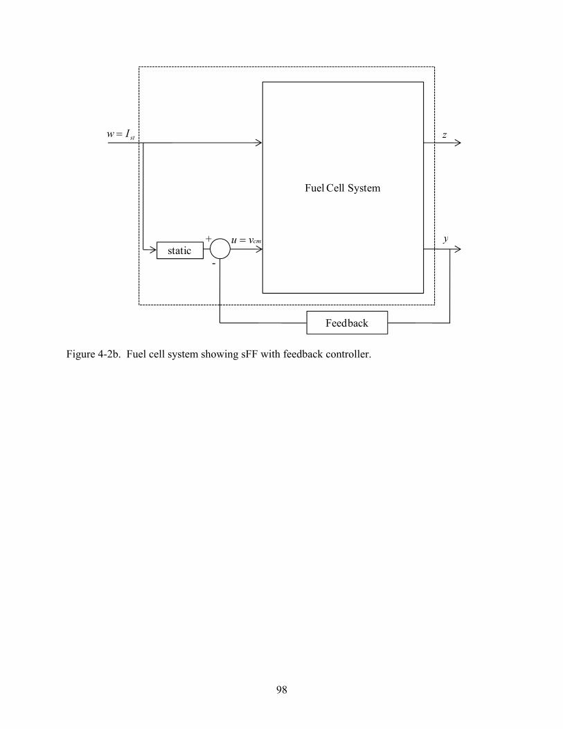
98
Fuel Cell System
stIw =
cmvu =
z
ystatic
Feedback
+
-
Figure 4-2b. Fuel cell system showing sFF with feedback controller.

99
A
-12.62 0 -10.95 0 8.4e-7 6e-18 0 2.4e-7 0 -315.8 0 0 1.004e-6 0 -35.34 0
-37.57 0 -46.31 -8.6e-24 2.76e-6 2e-17 0 1.58e-6 0 0 0 -17.19 0.2032 0 0 0
2.6e8 0 2.97e8 379.4 -38.7 1.06e7 0 0 33.28 0 38.03 4.834e-5 -4.8e-6 0 0 0
0 -295.6 0 0 9.33e-7 0 -63.61 0 4.045e8 0 4.621e8 0 0 0 0 -51.22
B
-3.16e-5 0 -3.98e-6 0
0 0 0 405.1 0 0 0 0
-5.245e-5 0 0 0
C
4.94e6 1.967e6 -1.089e5 2.066 0 0 0 0 -1273 0 -1454 -4.3e-22 1.388e-4 9.94e-16 0 0
0 0 0 4.834e-5 -1.16e-6 0 0 0 0 0 0 0 1 0 0 0
2.59e4 1.03e4 -569.9 0 0 0 0 0
D
180.2 -165.7 -0.01049 0
0 0 0 0
-0.2965 0
Figure 4-3. Matrices defining the LTI model for the fuel cell model excluding sFF.
A
-12.62 0 -10.95 0 8.4e-7 6e-18 0 2.4e-7 0 -315.8 0 0 1.004e-6 0 -35.34 0
-37.57 0 -46.31 -8.6e-24 2.76e-6 2e-17 0 1.58e-6 0 0 0 -36.8 0.2032 0 0 0
2.6e8 0 2.97e8 379.4 -38.7 1.06e7 0 0 33.28 0 38.03 4.834e-5 -4.8e-6 0 0 0
0 -295.6 0 0 9.33e-7 0 -63.61 0 4.045e8 0 4.621e8 0 0 0 0 -51.22
B
-3.16e-5 0 -3.98e-6 0
0 0 716.4 1065
0 0 0 0
-5.245e-5 0 0 0
C
4.94e6 1.967e6 -1.089e5 4.131 0 0 0 0 -1273 0 -1454 -4.3e-22 1.388e-4 9.94e-16 0 0
0 0 0 4.834e-5 -1.16e-6 0 0 0 0 0 0 0 1 0 0 0
2.59e4 1.03e4 -569.9 0 0 0 0 0
D
-112.9 -435.7 -0.01049 0
0 0 0 0
-0.2965 0
Figure 4-4. Matrices defining the LTI model for the fuel cell including sFF.

100
Fuel Cell System
stIw =
cmvu =
netPez =1
22 Oz λ=
cpWy =1
smpy =2
stvy =3
static
Figure 4-5. The sFF control configurations for fuel cell system.

101
(a)
Fuel Cell System
stIw =
cmvu =
netPez =1
22 Oz λ=
cpWy =1
smpy =2
stvy =3
dynamic
(b)
++uδ
uwK
wδwzG 2
uzG 2
2zδ
Figure 4-6. The dFF controller: (a)Schematic diagram, and (b)transfer function representation.

102
Fuel Cell System
stIw =
cmvu =
z
ysFF
Feedback
+
-
Figure 4-7. The sFF schematic with feedback controller.
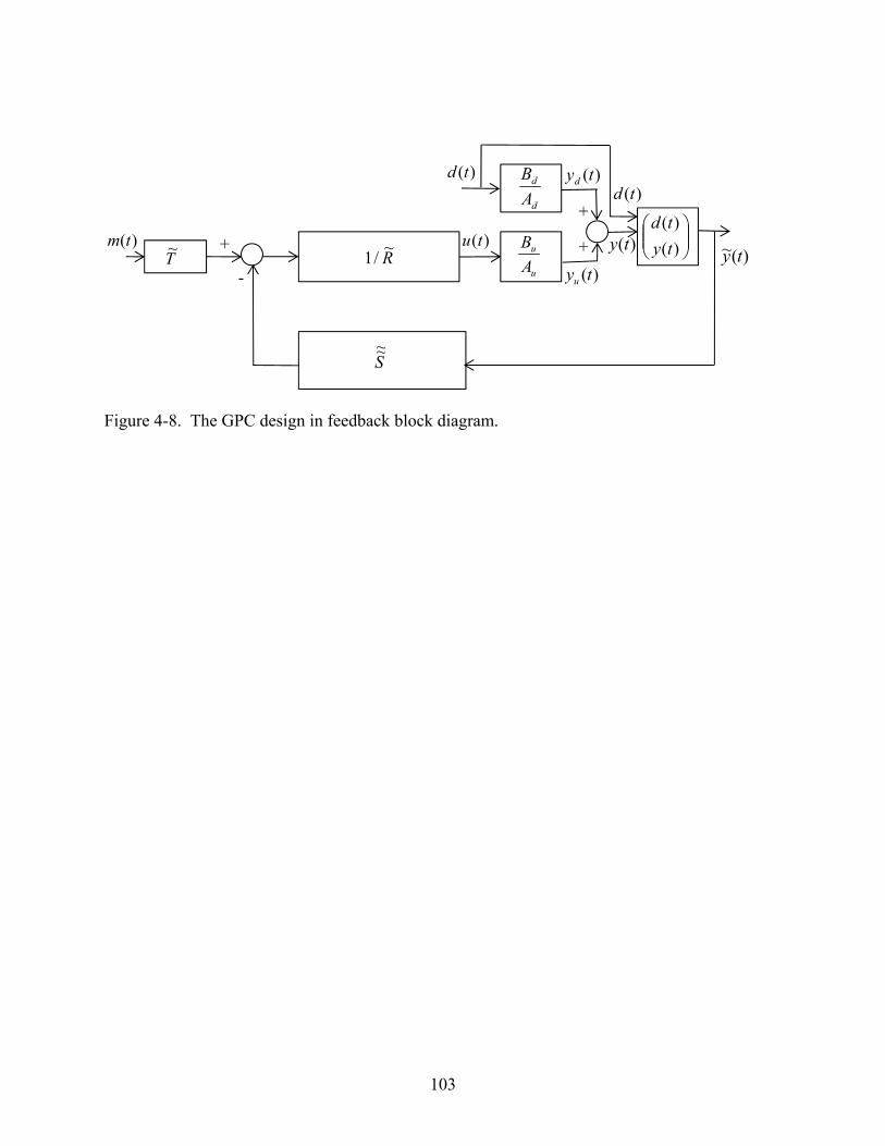
103
)(tu
)(td
)(tm)(~ ty
)(tyR~/1
S~~
T~
)(td
+
-
⎟⎟⎠
⎞⎜⎜⎝
⎛)()(
tytd
)(tyu
)(tyd
+
+
d
d
AB
u
u
AB
Figure 4-8. The GPC design in feedback block diagram.

104
0 5 10 15 20 25 3090
155
220
285
350
Time (sec)
Sta
ck C
urre
nt (
Am
p)
Figure 4-9. Disturbance profile used for simulation purposes.

105
0 5 10 15 20 25 301
1.2
1.4
1.6
1.8
2
2.2
2.4
2.6
2.8
Time (sec)
O2 E
xces
s R
atio
setpointGPC
Figure 4-10. The GPC control strategy implementation on the nonlinear fuel cell
model in the case when the controlled variable is measured.

106
0 5 10 15 20 25 301
1.2
1.4
1.6
1.8
2
2.2
2.4
2.6
2.8
Time (sec)
O2 E
xces
s R
atio
setpointGPC with 4 observers
Figure 4-11. The GPC feedback with four observers control scheme implementation
on the nonlinear fuel cell model.

107
0 5 10 15 20 25 300
2
4
6
8
10
12x 10
4
Time (sec)
Nor
m−
erro
r
Observer 1Observer 2Observer 3Observer 4
Figure 4-12. The Norm of errors from the battery of observers.

108
0 5 10 15 20 25 30
Obs 1
Obs 2
Obs 3
Obs 4
Time (sec)
Obs
erve
r se
lect
ed
Figure 4-13. The switching pattern of the battery of observers.
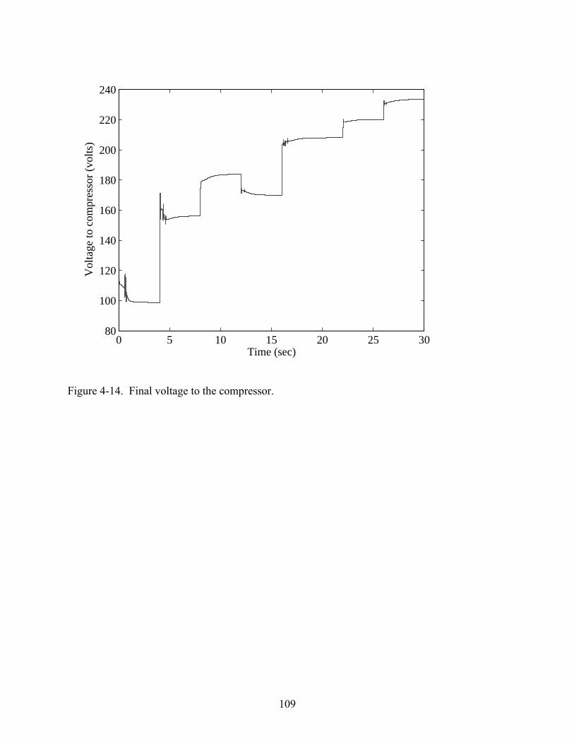
109
0 5 10 15 20 25 3080
100
120
140
160
180
200
220
240
Time (sec)
Vol
tage
to c
ompr
esso
r (v
olts
)
Figure 4-14. Final voltage to the compressor.

110
0 10 20 30−0.04
−0.02
0
0.02
0.04
Time (sec)
Wcp
err
or (
kg/s
)
zero errorObserver 1
0 10 20 30−2
0
2
4
6
8x 10
4
Time (sec)
Psm
err
or (
pasc
al)
zero errorObserver 1
0 10 20 30−5
0
5
10
15
20
Time (sec)
Vst
err
or (
volt)
zero errorObserver 1
Figure 4-15. Observer 1, error between measured and estimated values.

111
0 10 20 30−0.015
−0.01
−0.005
0
0.005
0.01
Time (sec)
Wcp
err
or (
kg/s
)
zero errorObserver 2
0 10 20 30−5000
0
5000
10000
15000
Time (sec)
Psm
err
or (
pasc
al)
zero errorObserver 2
0 10 20 30−4
−3
−2
−1
0
1
2
Time (sec)
Vst
err
or (
volt)
zero errorObserver 2
Figure 4-16. Observer 2, error between measured and estimated values.

112
0 10 20 30−0.02
−0.01
0
0.01
0.02
Time (sec)
Wcp
err
or (
kg/s
)
zero errorObserver 3
0 10 20 30−10
−5
0
5x 10
4
Time (sec)
Psm
err
or (
pasc
al)
zero errorObserver 3
0 10 20 30−20
−15
−10
−5
0
5
Time (sec)
Vst
err
or (
volt)
zero errorObserver 3
Figure 4-17. Observer 3, error between measured and estimated values.

113
0 10 20 30−0.03
−0.02
−0.01
0
0.01
Time (sec)
Wcp
err
or (
kg/s
)
zero errorObserver 4
0 10 20 30−15
−10
−5
0
5x 10
4
Time (sec)
Psm
err
or (
pasc
al)
zero errorObserver 4
0 10 20 30−40
−30
−20
−10
0
10
Time (sec)
Vst
err
or (
volt)
zero errorObserver 4
Figure 4-18. Observer 4, error between measured and estimated values.

114
0 5 10 15 20 25 301
1.2
1.4
1.6
1.8
2
2.2
2.4
2.6
2.8
Time (sec)
O2 E
xces
s R
atio
setpointGPC with 3 observers
Figure 4-19. The GPC feedback with three observers control scheme implementation
on the nonlinear fuel cell model.

115
0 5 10 15 20 25 301
1.2
1.4
1.6
1.8
2
2.2
2.4
2.6
2.8
Time (sec)
O2 E
xces
s R
atio
setpointGPC with 2 observers
Figure 4-20. The GPC feedback with two observers control scheme implementation
on the nonlinear fuel cell model.

116
0 5 10 15 20 25 301
1.2
1.4
1.6
1.8
2
2.2
2.4
2.6
2.8
Time (sec)
O2 E
xces
s R
atio
setpointGPC with 1 observer
Figure 4-21. The GPC feedback with one observer control scheme implementation on
the nonlinear fuel cell model.

117
0 5 10 15 20 25 301
1.2
1.4
1.6
1.8
2
2.2
2.4
2.6
2.8
Time (sec)
O2 E
xces
s R
atio
setpointGPC
Figure 4-22. The GPC control strategy implementation on the nonlinear fuel cell
model with a parameter changed from the value used for control design.

118
0 5 10 15 20 25 301
1.2
1.4
1.6
1.8
2
2.2
2.4
2.6
2.8
Time (sec)
O2 E
xces
s R
atio
setpointGPC with observer
Figure 4-23. The GPC controller with the LQG observer control strategy
implementation on the altered nonlinear fuel cell model.

119
0 5 10 15 20 25 301
1.2
1.4
1.6
1.8
2
2.2
2.4
2.6
2.8
Time (sec)
O2 E
xces
s R
atio
setpointGPC with 4 observers
Figure 4-24. The GPC controller with the 4 observers control strategy implementation
on the altered nonlinear fuel cell model.

120
0 5 10 15 20 25 301
1.2
1.4
1.6
1.8
2
2.2
2.4
2.6
2.8
Time (sec)
O2 E
xces
s R
atio
setpointGPCsFF with LQR
Figure 4-25. Comparison of the GPC control strategy with the sFF controller
combined with LQR feedback strategy on the unaltered nonlinear fuel cell model when the performance variable is measurable.

121
0 5 10 15 20 25 301
1.2
1.4
1.6
1.8
2
2.2
2.4
2.6
2.8
Time (sec)
O2 E
xces
s R
atio
setpointGPC with observersFF with LQG observer and LQR
Figure 4-26. The sFF with the LQG observer and LQR feedback, compared to GPC
with the LQG Observer control strategy implementation on the unaltered nonlinear fuel cell model when the performance variable is not measurable.

122
0 5 10 15 20 25 301
1.2
1.4
1.6
1.8
2
2.2
2.4
2.6
2.8
Time (sec)
O2 E
xces
s R
atio
setpointGPC with 4 observerssFF with LQG observer and LQR
Figure 4-27. The sFF with the LQG observer and LQR feedback, compared to GPC
with the 4 observers control strategy implementation on the unaltered nonlinear fuel cell model when the performance variable is not measurable.

123
0 5 10 15 20 25 301
1.2
1.4
1.6
1.8
2
2.2
2.4
2.6
2.8
Time (sec)
O2 E
xces
s R
atio
setpointGPCsFF with LQR
Figure 4-28. The sFF with the LQR feedback, compared to GPC, when performance
variable is measurable on the altered nonlinear fuel cell model.

124
0 5 10 15 20 25 301
1.2
1.4
1.6
1.8
2
2.2
2.4
2.6
2.8
Time (sec)
O2 E
xces
s R
atio
setpointGPC with observersFF with LQG observer and LQR
Figure 4-29. The sFF with the LQG observer and the LQR feedback compared to the
GPC with the LQG observer control strategy on the altered nonlinear fuel cell model.

125
0 5 10 15 20 25 301
1.2
1.4
1.6
1.8
2
2.2
2.4
2.6
2.8
Time (sec)
O2 E
xces
s R
atio
setpointGPC with 4 observerssFF with LQG observer and LQR
Figure 4-30. The sFF with the LQG observer and the LQR feedback compared to the
GPC with the 4 observers control strategy on the altered nonlinear fuel cell model.

126
0 5 10 15 20 25 301
1.2
1.4
1.6
1.8
2
2.2
2.4
2.6
2.8
Time (sec)
O2 E
xces
s R
atio
setpointGPCdFFsFF
Figure 4-31. The sFF and dFF strategies and the GPC control strategy, performance
compared when applied on the unaltered nonlinear fuel cell model.

127
0 5 10 15 20 25 301
1.2
1.4
1.6
1.8
2
2.2
2.4
2.6
2.8
Time (sec)
O2 E
xces
s R
atio
setpointGPC with observerdFFsFF
Figure 4-32. The sFF and dFF strategies and the GPC control strategy with the LQG observer, performance compared when applied on the unaltered nonlinear fuel cell model.

128
0 5 10 15 20 25 301
1.2
1.4
1.6
1.8
2
2.2
2.4
2.6
2.8
Time (sec)
O2 E
xces
s R
atio
setpointGPC with 4 observersdFFsFF
Figure 4-33. The performances of the sFF and dFF strategies and the GPC with the 4 observers control strategy compared when applied on the unaltered nonlinear fuel cell model.

129
0 5 10 15 20 25 301
1.2
1.4
1.6
1.8
2
2.2
2.4
2.6
2.8
Time (sec)
O2 E
xces
s R
atio
setpointGPCdFFsFF
Figure 4-34. The sFF and dFF strategies and the GPC control strategy, performance
compared when applied on the altered nonlinear fuel cell model.

130
0 5 10 15 20 25 301
1.2
1.4
1.6
1.8
2
2.2
2.4
2.6
2.8
Time (sec)
O2 E
xces
s R
atio
setpointGPC with observerdFFsFF
Figure 4-35. The sFF and dFF strategies and the GPC control strategy with the LQG
observer, performance compared when applied on the altered nonlinear fuel cell model.

131
0 5 10 15 20 25 301
1.2
1.4
1.6
1.8
2
2.2
2.4
2.6
2.8
Time (sec)
O2 E
xces
s R
atio
setpointGPC with 4 observersdFFsFF
Figure 4-36. The performance of sFF and dFF strategies and the GPC with 4 observers
control strategy compared when applied on the altered nonlinear fuel cell model.

132
CHAPTER 5 CONCLUSIONS AND PROPOSITIONS FOR FUTURE WORK
5.1 Conclusions
A Virtual Control Lab (VCL) with an inverted pendulum that can be utilized as a tool for
enhanced learning is described. The VCL can be used in conjunction with a process control
lecture for demonstrating various advanced concepts or can be used by students located in
geographically remote places. The animation module of the VCL allows the user to visually
observe the impact of the control design. The VCL can potentially minimize the problem of
scheduling laboratory time for physical equipment.
The problem of tracking the slope of ramp is examined. On the basis of results obtained, a
PI controller using the ITAE as the optimizing metric demonstrates the best results. The
controller performance is better than that of controllers proposed in literature. Tuning
relationships for PI and PI2 controllers, using three different optimizing metrics and 20,000
different plants is presented.
An elegant solution is proposed for the problem of fuel cell control by implementing a
GPC strategy which incorporates disturbance measurements to produce a manipulated variable.
The GPC design demonstrates better performance compared to control strategies available in
prior literature. The GPC controller results in zero offset in the performance variable in the
nonlinear model when the performance variable is measured. The GPC controller is also the best
performing controller when evaluated for model uncertainty. The controller exhibits zero offset,
showing its strength from a viewpoint of robustness, when employed on a modified model. In
the case when the performance variable is not measurable, a battery of observers is implemented
to estimate the value of the performance variable deliver the best result. However, the
robustness problems still exist.

133
5.2 Future Work
To validate the benefits and effectiveness, it is proposed that the VCL is tested as a pilot
teaching tool in process control classes taught at both undergraduate and graduate levels. The
feedback obtained from the instructors and students will be highly beneficial in improving and
incorporating features that could enhance the learning experience. It would be desirable to add
to the VCL a few more advanced control strategies such as the GPC approach.
For future work regarding the ramp tracking problem it is proposed to validate the
simulation results for physical setups that can take advantage of the tuning relationships
presented. It is also suggested to conduct a more comprehensive study to minimize the scatter in
the optimizing metric error for low θ/τ values of the ratio, that is, for systems with little dead
time.
For future work on the fuel cell control problem it is proposed to evaluate the design of
observers which take model uncertainty into account. A battery of observers can be designed at
each operating point, with each observer corresponding to a linearized model obtained from
different values of parameters. Then a bumpless switching strategy could be designed to select
an appropriate state estimate to feed to the controller. The experimental implementation of the
control scheme in a physical fuel cell may be of significant value to confirm or refine the results
discussed in this dissertation.

134
APPENDIX A OFFSET BETWEEN AUXILLIARY AND ORIGINAL RAMP
The final value theorem is used to calculate the shift between the original ramp and the
modified ramp. The transfer function for the process with time delay is given by
sp e
sKG θ
τ−
+=
1 (A-1)
and the transfer function for PI controller is given by
⎟⎟⎠
⎞⎜⎜⎝
⎛+=
sKG
Icc τ
11 (A-2)
and the equation for ramp in the time domain is
ttr α=)( (A-3)
Performing the Laplace transform of Eq. A-3, with the initial condition 0)0( ==tr , yields
2)(s
sr α= (A-4)
Using Eqs. A-1 and A-2, it is possible to derive the following standard closed loop
relationship between the output y and the ramp r :
)(1
)( srGG
GGsy
cp
cp
+= (A-5)
Now consider the error
)()()( tytrte −= (A-6)
defined as the difference between the set point and output. Applying final value theorem
( ))()(lim)(lim0
sysrstest
−=→∞→
(A-7)
and inserting Eq. A-4 and A-5 in Eq. A-7 yields

135
⎟⎟⎠
⎞⎜⎜⎝
⎛
+−=
→∞→ 220 1lim)(lim
sGGGG
sste
cp
cp
st
αα (A-8)
or cp
st GGste
+=
→∞→ 11lim)(lim
0
α (A-9)
Inserting Eq. A-1 and Eq. A-2 in Eq. A-9 results in
⎟⎟⎠
⎞⎜⎜⎝
⎛+
++
=−
→∞→
sKe
sKs
te
Ic
sst
ττ
α
θ 111
1
1lim)(lim0
(A-10)
Simplifying terms and applying the limits on the right hand side of Eq. A-10 yields
Ic
tKK
te
τ
α1
1)(lim =∞→
(A-11)
Hence, c
I
t KKte ατ=
∞→)(lim (A-12)
which is an analytical expression for the offset between the auxiliary and the original ramp.

136
APPENDIX B OBSERVER DESIGN USING TRANSFER FUNCTION
The observer equations are given by
)ˆ(ˆˆ xCyLBuxAx −++= (B-1)
DuxCy += ˆˆ (B-2)
Eq. B-1 can be re-written as
LyBuxLCAx ++−= ˆ)(ˆ (B-3)
Performing Laplace Transform
)()()(ˆ)()0(ˆ)(ˆ sLYsBUsXLCAtxsXs ++−==− (B-4)
This results
)0(ˆ)()()(ˆ)( =++=+− txsLYsBUsXLCAsI (B-5)
On further manipulation
)0(ˆ)()()(ˆ =++= txMsMLysMBusx (B-6)
where 1)( −+−= LCAsIM
Now if
xCz z ˆˆ = (B-7)
)0(ˆ)()()(ˆ =++= txMCsMLYCsMBUCsZ zzz (B-8)
)0(ˆ)()()(ˆ)(ˆˆˆˆ XGsYGsUGsZ oxzyzuz ++= (B-9)
where MBCG zuz =ˆ , MLCG zyz =ˆ , and MCG zxz =)0(ˆˆ .

137
LIST OF REFERENCES
1. T. F. Junge and C. Schmid, Web-based remote experimentation using a laboratory-scale optical tracker, Proceedings of the American Control Conference, Chicago Illinois, June 2000.
2. D. Gillet, C. Salzmann, R. Longchamp, and D. Bonvin, Telepresence: an opportunity to develop practical experimentation in automatic control education, European Controls Conference, Brussels Belgium, July 1997.
3. D. Gillet, F. Geoffroy, K. Zeramdini, A. V. Nguyen, Y. Rekik and Y. Piguet, The cockpit: An effective metaphor for Web-based experimentation in engineering education, International Journal of Engineering Education, 19(3), August 2002, pp. 389-397.
4. D. Gillet, G. Fakas, eMersion: a new paradigm for Web-based training in engineering education, International Conference on Engineering Education, Oslo, Norway, 2001, 84B-10.
5. A. Bhandari, M. H. Shor, Access to an instructional control laboratory experiment through the World Wide Web, Proceedings of the American Control Conference, Philadelphia, June 1998.
6. Ch. Schmid, T.I. Eikass, B. Foss and D. Gillet, A remote laboratory experimentation network, 1st IFAC Conference on Telematics Applications in Automation and Robotics, Weingarten, Germany, July 24-26, 2001.
7. H. Latchman, C. Salzmann, S. Thotapilly and H. Bouzekri, Hybrid asynchronous and synchronous learning networks in distance education, International Conference on Engineering Education, Rio de Janeiro, Brazil, 1998.
8. B. Armstrong and R. Perez, controls laboratory program with an accent on discovery learning, IEEE Control Systems Magazine, February 2001, pp. 14-20.
9. J. W. Overstreet and A. Tzes, Internet-based client/server virtual instruments designs for real time remote-access control engineering laboratory, Proceedings of the American Control Conference, San Diego, 1999.
10. C. Schmid, The virtual control lab VCLab for education on the Web, Proceedings of the American Control Conference, Philadelphia, June 1998.
11. O. D. Crisalle and H. A. Latchman, Virtual control laboratory for multidisciplinary engineering education, NSF Award No. DUE-9352523, proposal funded by the National Science Foundation under the Instrumentation and Laboratory Improvement Program, (1993).
12. C. S. Peek; O. D. Crisalle; S. Depraz and D. Gillet, The virtual control laboratory paradigm: Architectural design requirements and realization through a DC-motor example, International Journal of Engineering Education, 21(6), 2005, pp. 1134-1147

138
13. National Instruments Corp., 11500 N. Mopac Expressway, Austin, TX 78759-3504, USA, www.ni.com.
14. M. W. Dunnigan, Enhancing state-space control teaching with a computer-based assignment, IEEE Transactions on Education,44(2), May 2001, pp. 129-136.
15. P. C. Wankat and F. S. Oreovicz, Teaching Engineering, McGraw-Hill, (1993).
16. A. M. Lopez; J. A. Miller, C. L. Smith and P. W. Murrill, Tuning controllers with error-integral criteria, Instrumentation Technology, 14(11), November 1967, pp. 57-62.
17. C. Smith and A. Corripio, Principles and Practice of Automation Control. J. Wiley. (1997).
18. W. Brogan, Modern Control Theory, 4th edn, Prentice-Hall, (1991).
19. P. W. Belanger and W. L. Luyben, Design of low-frequency compensator for improvement of plantwide regulatory performance, Ind. Eng. Chem. Res., 36, 1997, pp. 5339-5347.
20. R. Monroy-Loperena, I. Cervantes, A. Morales and J. Alvarez-Ramirez, Robustness and parametrization of the proportional plus double-integral compensator, Ind. Eng. Chem. Res. 38, 1999, pp. 2013-2020.
21. C. S. Peek, Development of virtual control laboratories for control engineering education, double integral controllers for ramp tracking and predictive control for robust control and luenberger observers, PhD Candidacy Exam, Dept. of Chemical Engineering, College of Engineering, University of Florida; 2006.
22. Mathworks Inc. MATLAB. Version 7.2.0.232, R2006a (2006).
23. S. Davis, Transportation Energy Data Book, 20th edn, U. S. Department of Energy, (2000).
24. W. Grove, A small voltaic battery of great energy, Philosophical Magazine, 15, 1839, pp. 287-293.
25. J. Amphlett, R. Baumert, R. Mann, B. Peppley, P. Roberage and A. Rodrigues, Parametric modelling of the performance of a 5-kW proton-exchange membrane fuel cell stack, Journal of Power Sources, 49, 1994, pp. 349-356.
26. J. Amphlett, R. Baumert, R. Mann, B. Peppley and P. Roberage, Performance modeling of the Ballard Mark IV solid polymer electrolyte fuel cell, Journal of Electrochemical Society, 142(1), 1995, pp. 9-15.
27. D. Bernardi, Water-balance calculations for solid-polymer-electrolyte fuel cells, Journal of Electrochemical Society, 137(11), 1990, pp. 3344-3350.
28. D. Bernardi and M. Verbrugge, A mathematical model of the solid-polymer-electrolyte fuel cell, Journal of Electrochemical Society, 139(9), 1992, pp. 2477-2491.

139
29. J. Baschuk and X. Li, Modelling of polymer electrolyte membrane fuel cells with variable degrees of water flooding, Journal of Power Sources, 86, 2000, pp. 186-191.
30. J. Eborn, L. Pedersen, C. Haugstetter and S. Ghosh, System level dynamic modeling of fuel cell power plants, Proceedings of the American National Conference, 2003, pp. 2024-2029.
31. J. T. Pukrushpan, A. G. Stefanopoulou and H. Peng, Control of fuel cell power systems: principles, modeling, analysis and feedback design, Advances in Industrial Control. Springer-Verlag London Limited, (2004).
32. D. Seborg, T. Edgar and D. Mellichamp, Process Dynamics and Control, 2nd edn, Wiley, (2004).
33. K. Ogata, Modern Control Engineering, 4th edn, Prentice Hall, (2001).
34. R. Stefani, B. Shahian, C. Savant and G. Hostetter, Design of Feedback Control Systems, 4th edn, Oxford University Press, (2002).
35. O. D. Crisalle, D. E. Seborg and D. A. Mellichamp, Theoretical analysis of long-range predictive controllers, Proceedings of the American Control Conference, Pittsburgh, Pennsylvania, 1989.
36. D. W. Clarke, C. Mohtadi and P. S. Tufts, Generalized predictive control – part I. The basic algorithm, Automatica, 23(2), 1987, pp. 137-148.
37. D. W. Clarke, C. Mohtadi and P. S. Tufts, Generalized predictive control – part II. Extensions and interpretations, Automatica, 23(2), 1987, pp. 149-160.
38. D. W. Clarke and C. Mohtadi, Properties of generalized predictive control, Automatica, 25(6), 1989, pp. 859-875.

BIOGRAPHICAL SKETCH
Vikram Shishodia was born in Delhi, India. He graduated with a B.Tech. in chemical
engineering from the Indian Institute of Technology Delhi in 1992. Mr. Vikram Shishodia
joined the graduate program at the University of Florida in 1993. He graduated with an M.S. in
materials science and engineering in 1996. After developing a successful career as a process
engineer with Intel Corporation for nine years he returned to academia to pursue higher degrees
in chemical engineering at the University of Florida. From 2005 to 2008 he was a graduate
student and simultaneously worked as Assistant Director for the Division of Student Affairs at
the College of Engineering of University of Florida. He graduated with an M.S. in chemical
engineering in 2003 and a Ph.D. in chemical engineering from the University of Florida in 2008.