university of derby a novel approach to the … · a novel approach to the control of . quad-rotor...
TRANSCRIPT

A novel approach to the control of quad-rotor helicopters usingfuzzy-neural networks
Item type Thesis or dissertation
Authors Poyi, Gwangtim Timothy
Publisher University of Derby
Downloaded 15-Jul-2018 13:40:40
Link to item http://hdl.handle.net/10545/337911

UNIVERSITY OF DERBY
A NOVEL APPROACH TO THE CONTROL OF
QUAD-ROTOR HELICOPTERS USING
FUZZY-NEURAL NETWORKS
GWANGTIM TIMOTHY POYI
Doctor of Philosophy 2014
ii
ABSTRACT
Quad-rotor helicopters are agile aircraft which are lifted and propelled by four rotors. Unlike
traditional helicopters, they do not require a tail-rotor to control yaw, but can use four smaller
fixed-pitch rotors. However, without an intelligent control system it is very difficult for a
human to successfully fly and manoeuvre such a vehicle. Thus, most of recent research has
focused on small unmanned aerial vehicles, such that advanced embedded control systems
could be developed to control these aircrafts. Vehicles of this nature are very useful when it
comes to situations that require unmanned operations, for instance performing tasks in
dangerous and/or inaccessible environments that could put human lives at risk.
This research demonstrates a consistent way of developing a robust adaptive controller for
quad-rotor helicopters, using fuzzy-neural networks; creating an intelligent system that is able
to monitor and control the non-linear multi-variable flying states of the quad-rotor, enabling it
to adapt to the changing environmental situations and learn from past missions.
Firstly, an analytical dynamic model of the quad-rotor helicopter was developed and
simulated using Matlab/Simulink software, where the behaviour of the quad-rotor helicopter
was assessed due to voltage excitation. Secondly, a 3-D model with the same parameter
values as that of the analytical dynamic model was developed using Solidworks software.
Computational Fluid Dynamics (CFD) was then used to simulate and analyse the effects of
the external disturbance on the control and performance of the quad-rotor helicopter.
Verification and validation of the two models were carried out by comparing the simulation
results with real flight experiment results. The need for more reliable and accurate simulation
data led to the development of a neural network error compensation system, which was
embedded in the simulation system to correct the minor discrepancies found between the
simulation and experiment results.
Data obtained from the simulations were then used to train a fuzzy-neural system, made up of
a hierarchy of controllers to control the attitude and position of the quad-rotor helicopter. The
success of the project was measured against the quad-rotor’s ability to adapt to wind speeds
of different magnitudes and directions by re-arranging the speeds of the rotors to compensate
for any disturbance. From the simulation results, the fuzzy-neural controller is sufficient to
achieve attitude and position control of the quad-rotor helicopter in different weather
conditions, paving way for future real time applications.
iii
ACKNOWLEDGEMENTS
My profound gratitude goes to God Almighty for the courage, wisdom and focus I had
throughout the period of this research despite all the turbulence. It was like walking on the
edge of a cliff in the midst of a hurricane, but not for a moment did He forsake me. He found
me right in the middle of the hurricane and helped me get through successfully.
The academic guidance and support received from my Supervisory Team was the greatest.
There couldn’t have been a better team than the one made up of Prof Mian Hong Wu, Dr
Amar Bousbaine (both of University of Derby) and Prof Huosheng Hu (of the University of
Essex). Thank you for all the support and encouragement.
My thanks also go to the Head, School of Engineering and Technology - Angela Dean and
the ADT Faculty Research Manager - Prof Neil Campbell, thank you both for standing by me
when I needed help. To the Subject Head of Electronics and Sound - Tim Wilmshurst, thanks
for all the encouragement.
I am grateful to Isobel Manning, Jessamie Self and all staff of the University Research
Office. My friends and colleagues – John Oyekan and Bowen Lu (University of Essex),
Sugiono Sugiono, and Ali Salem Al-Aref, many thanks for your contributions when I was
building my models and collecting flight experiment data.
My appreciation also goes to TETFUND-Nigeria for the funding provided for my studies and
to FCE – Pankshin for the leave period granted for my studies. I’m indebted to Mr Emmanuel
Manasa – thank you for standing by me right from the beginning of the ‘PhD storm’.
To members of my family – Mr and Mrs Venmah Poyi (my Parents), Gwahzin, Dr and Mrs
Victor Gimba, Nanfe, Victor, Jesse and Michelle – thank you all for your unreserved support,
encouragement and prayers through the storm of my PhD research. I know it wasn’t easy for
all of us.
To Prof Ugbo Mallam and Dr Gideon Dala, thank you for your support and encouragement at
the most crucial times – that went a long way. Many thanks to Mr Amos Bulus Cirfat, Jo-
Kim Sharon, Sallau Nanlir Mullah and others too numerous to mention, who have
contributed in one way or the other to the success of my PhD research. May God continue to
bless and keep you all.

iv
TABLE OF CONTENTS ABSTRACT ............................................................................................................................................ ii
ACKNOWLEDGEMENTS ................................................................................................................... iii
LIST OF FIGURES ............................................................................................................................... ix
LIST OF TABLES ............................................................................................................................... xiii
NOMENCLATURE .............................................................................................................................xiv
CHAPTER 1 ........................................................................................................................................... 1
INTRODUCTION .................................................................................................................................. 1
1.0 Unmanned Aerial Vehicles (UAVs) ................................................................................................. 2
1.1 The Miniature Quad-rotor Unmanned Aerial Vehicle ...................................................................... 3
1.2 Anatomy of the Quad-rotor Helicopter ............................................................................................. 4
1.2.1 Frame ..................................................................................................................................... 4
1.2.2 Landing Gear ......................................................................................................................... 5
1.2.3 Motors and Propellers ............................................................................................................ 6
1.2.4 Battery .................................................................................................................................... 6
1.2.5 Sensors ................................................................................................................................... 7
1.2.6 Flight Control Board .............................................................................................................. 9
1.2.7 Transmitter and Receiver ....................................................................................................... 9
1.3 Basic concepts of the quad-rotor helicopter .................................................................................... 11
1.3.1 Throttle ................................................................................................................................. 12
1.3.2 Roll ....................................................................................................................................... 13
1.3.3 Pitch ..................................................................................................................................... 13
1.3.4 Yaw ...................................................................................................................................... 14
1.4 Applications of Miniature Quad-rotor Helicopters ......................................................................... 15
1.4.1 Border Patrol ........................................................................................................................ 15
1.4.2 Disaster Management/ Search and Rescue .......................................................................... 16
1.4.3 Wild fire detection ............................................................................................................... 18
1.4.4 Photography ......................................................................................................................... 19
1.4.5 Military and Law enforcement ............................................................................................. 20
1.4.6 Research ............................................................................................................................... 20
1.4.7 Agricultural and Industrial applications ............................................................................... 21
1.5 Chapter Summary ........................................................................................................................... 23
CHAPTER 2 ......................................................................................................................................... 24
STATE OF THE ART AND KEY RESEARCH REVIEWS ............................................................... 24

v
2.0 Previous works on the quad-rotor helicopter .................................................................................. 25
2.1 The basics concepts of Computational Fluid Dynamics (CFD) ...................................................... 31
2.1.1 Applications of Computational Fluid Dynamics (CFD) in Aircraft Control ....................... 33
2.2 The basic concepts of Artificial Neural Networks .......................................................................... 34
2.2.1 Applications of Artificial Neural Networks in Aircraft Control .......................................... 36
2.3 The basics concepts of Fuzzy Logic ............................................................................................... 37
2.3.1 Applications of Fuzzy Logic in Aircraft Control ................................................................. 39
2.4 Aim and Objectives of the research project .................................................................................... 40
2.5 Choosing a Control Technique ....................................................................................................... 40
2.5.1 Capabilities of Fuzzy- Neural Systems ................................................................................ 41
2.6 Contributions of this work .............................................................................................................. 42
2.7 Thesis layout ................................................................................................................................... 43
2.8 Chapter Summary ........................................................................................................................... 44
CHAPTER 3 ......................................................................................................................................... 46
ANALYTICAL DYNAMIC MODEL OF THE QUAD-ROTOR ....................................................... 46
3.0 The Newton-Euler model ................................................................................................................ 47
3.0.1 Coordinate Frames ............................................................................................................... 48
3.0.2 Quad-rotor Modelling Assumptions .................................................................................... 49
3.0.3 Quad-rotor Helicopter State Variable definition .................................................................. 50
3.0.4 Direction Cosine Matrix....................................................................................................... 52
3.0.5 Quad-rotor Kinematics ......................................................................................................... 54
3.0.6 Quad-rotor Dynamics ........................................................................................................... 55
3.0.7 Quad-rotor Aerodynamic Forces ......................................................................................... 59
3.0.8 Quad-rotor Moments (Torques) ........................................................................................... 62
3.0.9 Quad-rotor Moments of Inertia ............................................................................................ 62
3.0.10 Equations of Motion........................................................................................................... 64
3.1 Actuator Dynamics (DC-motor) ..................................................................................................... 66
3.1.1 Voltage and Angular Velocity of Propeller ......................................................................... 68
3.1.2 Voltage and Thrust ............................................................................................................... 69
3.1.3 Rolling Moment ................................................................................................................... 71
3.1.4 Pitching Moment .................................................................................................................. 72
3.1.5 Yawing Moment .................................................................................................................. 72
3.1.6 Acceleration along the x-axis ............................................................................................... 73
3.1.7 Acceleration along the y-axis ............................................................................................... 73

vi
3.1.8 Acceleration along z-axis ..................................................................................................... 74
3.2 Chapter Summary ........................................................................................................................... 75
CHAPTER 4 ......................................................................................................................................... 76
SIMULATION OF THE QUAD-ROTOR ANALYTICAL DYNAMIC MODEL IN MATLAB/SIMULINK ......................................................................................................................... 76
4.0 Matlab/Simulink Software .............................................................................................................. 77
4.1 Model Implementation in Matlab/Simulink .................................................................................... 78
4.1.1 Summary of equations of motion ......................................................................................... 78
4.1.2 Actuator Subsystem ............................................................................................................. 79
4.1.3 Roll Subsystem .................................................................................................................... 80
4.1.4 Pitch Subsystem ................................................................................................................... 80
4.1.5 Yaw Subsystem .................................................................................................................... 81
4.1.6 X-Motion Subsystem ........................................................................................................... 82
4.1.7 Y-Motion Subsystem ........................................................................................................... 82
4.1.8 Z-Motion Subsystem ............................................................................................................ 83
4.2 Running the Simulation .................................................................................................................. 84
4.2.1 Calibration and Preliminary Calculations ............................................................................ 84
4.2.2 Hover .................................................................................................................................... 89
4.2.3 Throttle (Vertical Motion) ................................................................................................... 89
4.2.4 Roll ....................................................................................................................................... 91
4.2.5 Pitch ..................................................................................................................................... 95
4.2.6 Yaw ...................................................................................................................................... 99
4.3 Chapter Summary ......................................................................................................................... 102
CHAPTER 5 ....................................................................................................................................... 103
QUAD-ROTOR 3-D CAD MODEL AND COMPUTATIONAL FLUID DYNAMICS (CFD) SIMULATION .................................................................................................................................... 103
5.0 Quad-rotor Helicopter CFD .......................................................................................................... 104
5.1 Quad-rotor 3-D CAD Model ......................................................................................................... 108
5.2 CFD Flow Solver .......................................................................................................................... 110
5.3 Analysis of CFD results ................................................................................................................ 112
5.3.1 Results of CFD simulation in a no wind situation ............................................................. 113
5.3.2 Results of CFD simulation in windy situations .................................................................. 119
5.4 Chapter Summary ......................................................................................................................... 127
CHAPTER 6 ....................................................................................................................................... 128
VALIDATION OF MODELS WITH FLIGHT EXPERIMENT DATA ........................................... 128
vii
6.0 Verification and Validation ........................................................................................................... 129
6.1 Flight Experiments with the Quad-rotor helicopter ...................................................................... 130
6.1.1 Experimental Set-up in the Robot Arena ........................................................................... 130
6.1.2 Comparison of results ........................................................................................................ 132
6.2 Error Compensation using Artificial Neural Networks ................................................................ 137
6.2.1 Compensation Architecture ................................................................................................ 137
6.3 Chapter Summary ......................................................................................................................... 140
CHAPTER 7 ....................................................................................................................................... 142
INTELLIGENT CONTROLLER DESIGN ........................................................................................ 142
7.0 Aircraft Navigation in the Wind ................................................................................................... 143
7.1 Neural Network Model ................................................................................................................. 144
7.1.1 Mathematical Model of a Neural Network ........................................................................ 145
7.2 Fuzzy Set Theory used in the Neural Network Model .................................................................. 149
7.2.1 Membership Functions ....................................................................................................... 150
7.2.2 If-Then Rules ..................................................................................................................... 151
7.3 Fuzzy-Neural Model for the Quad-rotor Helicopter ..................................................................... 152
7.4 Controller design ........................................................................................................................... 153
7.4.1 Attitude Controller ............................................................................................................. 158
7.4.2 Position Controller ............................................................................................................. 162
7.6 Chapter Summary ......................................................................................................................... 163
CHAPTER 8 ....................................................................................................................................... 164
SIMULATION RESULTS AND DISCUSSION ............................................................................... 164
8.0 Flight Controller Simulation ......................................................................................................... 165
8.1 Flight Simulation in No Wind Situation ....................................................................................... 166
8.2. Flight Simulation in a Headwind ................................................................................................. 168
8.2.1 Constant Headwind ............................................................................................................ 169
8.2.2 Gusty Headwind ................................................................................................................. 171
8.3 Flight Simulation in a Tailwind .................................................................................................... 173
8.3.1 Constant Tailwind .............................................................................................................. 173
8.3.2 Gusty Tailwind ................................................................................................................... 175
8.4 Flight Simulation in a Crosswind.................................................................................................. 177
8.4.1 Constant Crosswind ........................................................................................................... 177
8.4.2 Gusty Crosswind ................................................................................................................ 180
8.5 Discussion of Results .................................................................................................................... 182
viii
8.6 Towards Implementation .............................................................................................................. 183
8.7 Chapter Summary ......................................................................................................................... 186
CHAPTER 9 ....................................................................................................................................... 187
SUMMARY, CONCLUSION AND SUGGESTED AREAS OF FUTURE RESEARCH ................ 187
9.0 Summary of the Aim and Objectives of the Research .................................................................. 188
9.1 Research Summary and Conclusions ............................................................................................ 188
9.2 Suggested areas for future research .............................................................................................. 191
REFERENCES ................................................................................................................................... 193
APPENDIX A: MATLAB/SIMULINK MODEL .............................................................................. 201
APPENDIX B: QUAD-ROTOR SOLIDWORKS 3-D CAD MODEL .............................................. 203
APPENDIX C: SAMPLE OF MODEL SIMULATION RESULTS .................................................. 207
APPENDIX D: SAMPLE OF FLIGHT EXPERIMENT DATA ....................................................... 211
APPENDIX E: ADDITIONAL CONTROL SIMULATION RESULTS........................................... 214
APPENDIX F: LINEARIZATION OF QUAD-ROTOR MODEL .................................................... 220
APPENDIX G: FLIGHT SIMULATION DISPLAY PROGRAM .................................................... 228
APPENDIX H: LIST OF PUBLICATIONS ...................................................................................... 231
ix
LIST OF FIGURES
Figure 1-1: Quad-rotor helicopter frame ................................................................................................................ 5 Figure 1-2: Quad-rotor landing gear ....................................................................................................................... 5 Figure 1-3: Propeller mounted on a brushless DC motor ....................................................................................... 6 Figure 1-4: Battery.................................................................................................................................................. 7 Figure 1-5: Inertial measurement unit .................................................................................................................... 7 Figure 1-6: Flight control board ............................................................................................................................. 9 Figure 1-7: Transmitter-receiver ........................................................................................................................... 10 Figure 1-8: Quad-rotor helicopter ........................................................................................................................ 10 Figure 1-9: Simplified quad-rotor helicopter structure ......................................................................................... 11 Figure 1-10: Throttle command response ............................................................................................................. 12 Figure 1-11: Roll command response ................................................................................................................... 13 Figure 1-12: Pitch command response.................................................................................................................. 14 Figure 1-13: Yaw command response .................................................................................................................. 14 Figure 1-14: An image from a UAV on border patrol .......................................................................................... 16 Figure 1-15: UAV for search and rescue in the coastlines ................................................................................... 17 Figure 1-16: UAV for search and rescue in disaster situations in the Philippines ................................................ 18 Figure 1-17: Fire monitoring using a UAV and a thermal infrared scanner ......................................................... 19 Figure 1-18: Remote controlled helicopters fitted with cameras fly above Sydney ............................................. 19 Figure 1-19: UAVs assist the law enforcement agencies with tracking and aerial photography .......................... 20 Figure 1-20: Flight demo at University of Derby and the autonomous squadron from KMel Robotics ............... 21 Figure 1-21: A quad-rotor helicopter working alongside heavy farm equipment ................................................. 22 Figure 1-22: A quad-rotor helicopter used to monitor industrial installations ...................................................... 22 Figure 2-1: CFD application in automotive simulation and blood flow in the human body ................................ 32 Figure 2-2: CFD application in simulation of vortices around aircrafts ............................................................... 34 Figure 2-3: Artificial neural network model ......................................................................................................... 35 Figure 2-4: Artificial neural network model for UAV control ............................................................................. 37 Figure 2-5: A simple fuzzy logic application ....................................................................................................... 38 Figure 2-6: Fuzzy logic application in aircraft control ......................................................................................... 39 Figure 2-7: Overall Project Framework ................................................................................................................ 45 Figure 3-1: The quad-rotor axes definition ........................................................................................................... 48 Figure 3-2: Quad-rotor Configuration Scheme ..................................................................................................... 50 Figure 3-3: Rotation around the X axis of the angle ϕ (roll) .............................................................................. 52
Figure 3-4: Rotation around the Y axis of the angle θ (pitch) ............................................................................ 53 Figure 3-5: Rotation around the Z axis of the angle ψ (yaw) .............................................................................. 53 Figure 3-6: Quad-rotor moments of inertia ........................................................................................................... 63 Figure 3-7: Schematic of a DC Motor .................................................................................................................. 66 Figure 3-8: DC Motor circuit ................................................................................................................................ 67 Figure 3-9: Simplified DC motor system ............................................................................................................. 68 Figure 4-1: Open loop simulation system ............................................................................................................. 78 Figure 4-2: The Actuator (Electric Motor) Subsystem ......................................................................................... 80 Figure 4-3: The Roll Subsystem ........................................................................................................................... 80 Figure 4-4: The Pitch Subsystem .......................................................................................................................... 81 Figure 4-5: The Yaw Subsystem .......................................................................................................................... 81 Figure 4-6: X-Motion Subsystem. ........................................................................................................................ 82 Figure 4-7: Y-Motion Subsystem ......................................................................................................................... 83 Figure 4-8: The z-motion Subsystem.................................................................................................................... 83 Figure 4-9: Simulation results without proper configuration and calibration of the model .................................. 84 Figure 4-10: Electric motor response to operating voltage step input .................................................................. 88 Figure 4-11: Height reached at hover ................................................................................................................... 89 Figure 4-12: Height reached when each motor is given an input of 4.6volts ....................................................... 90

x
Figure 4-13: Upward velocity of quad-rotor helicopter ........................................................................................ 90 Figure 4-14: Total thrust generated at different motor speeds .............................................................................. 91 Figure 4-15: Roll angle ......................................................................................................................................... 92 Figure 4-16: Y-displacement as a result of roll angle ........................................................................................... 92 Figure 4-17: Components of forces as a result of the rolling moment .................................................................. 93 Figure 4-18: Position reached when rolling .......................................................................................................... 94 Figure 4-19: Forces acting on the helicopter as a result of different roll angles ................................................... 95 Figure 4-20: Pitch angle ....................................................................................................................................... 96 Figure 4-21: X-displacement as a result of pitch angle ........................................................................................ 97 Figure 4-22: Components of forces as a result of the pitching moment ............................................................... 97 Figure 4-23: Position reached when pitching ....................................................................................................... 98 Figure 4-24: Forces acting on the helicopter as a result of different pitch angles ................................................ 98 Figure 4-25: Yaw angle ........................................................................................................................................ 99 Figure 4-26: Z-displacement............................................................................................................................... 100 Figure 4-27: Components of forces as a result of the yawing moment............................................................... 100 Figure 4-28: Position reached when yawing ....................................................................................................... 101 Figure 4-29: Forces acting on the helicopter as a result of different yaw angles ................................................ 101 Figure 5-1: Air flows around the quad-rotor helicopter in a CFD simulation .................................................... 105 Figure 5-2: CFD mesh diagram .......................................................................................................................... 106 Figure 5-3: CFD process flow ............................................................................................................................ 107 Figure 5-4: SolidWorks 3-D model of the quad-rotor helicopter ....................................................................... 110 Figure 5-5: Flow-solver dialogue box ................................................................................................................ 110 Figure 5-6: Computational domain of CFD simulation ...................................................................................... 111 Figure 5-7: Air distribution around the rotors during simulation ....................................................................... 112 Figure 5-8: Flow-simulation dialogue box for changing rotor speeds ................................................................ 113 Figure 5-9: Flow-simulation dialogue box showing all wind speeds at 0m/s ..................................................... 113 Figure 5-10: Upward velocity of quad-rotor helicopter ...................................................................................... 114 Figure 5-11: Total thrust generated at different motor speeds ............................................................................ 115 Figure 5-12: Forces acting on the helicopter as a result of different roll angles ................................................. 115 Figure 5-13: Components of forces as a result of the roll moment ..................................................................... 116 Figure 5-14: Forces acting on the helicopter as a result of different pitch angles .............................................. 117 Figure 5-15: Components of forces as a result of the pitching moment ............................................................. 117 Figure 5-16: Components of forces as a result of the yawing moment............................................................... 118 Figure 5-17: Forces acting on the helicopter as a result of different yaw angles ................................................ 118 Figure 5-18: Dialogue box showing how the different wind speeds were set .................................................... 119 Figure 5-19: Calculating the effect of wind disturbance on the quad-rotor helicopter ....................................... 120 Figure 5-20: Impact of air flows on the performance of the quad-rotor helicopter ............................................ 121 Figure 5-21: Total vertical thrust in downward flow of wind ............................................................................. 122 Figure 5-22: Total vertical thrust in upward flow of wind ................................................................................. 122 Figure 5-23: Quad-rotor experiencing cross winds in simulation ....................................................................... 123 Figure 5-24: Forces acting on the helicopter in a headwind ............................................................................... 124 Figure 5-25: Forces acting on the helicopter in a headwind at different tilt angles ............................................ 124 Figure 5-26: Quad-rotor forces in a tailwind ...................................................................................................... 125 Figure 5-27: Quad-rotor forces in a crosswind blowing in the direction of tilt of the helicopter ....................... 126 Figure 5-28: Quad-rotor forces in a crosswind blowing against the direction of tilt of the helicopter ............... 126 Figure 5-29: Forces acting on the helicopter in a crosswind at different angles of tilt ....................................... 127 Figure 6-1: Verification and validation process flow ......................................................................................... 129 Figure 6-2: Hardware set-up for flight experiments ........................................................................................... 130 Figure 6-3: Quad-rotor flight data plot from the VICON data logging system .................................................. 133 Figure 6-4: Comparison of results in throttle test ............................................................................................... 133 Figure 6-5: Comparison of simulated and measured roll and pitch angles ......................................................... 134 Figure 6-6: Comparison of simulated and measured forces in roll and pitch tests ............................................. 135

xi
Figure 6-7: Comparison of simulated and measured yaw angles ....................................................................... 136 Figure 6-8: Comparison of simulated and measured forces as a result of different yaw angles ......................... 136 Figure 6-9: Artificial neural network correction system ..................................................................................... 138 Figure 7-1: Navigation vector relationship ......................................................................................................... 143 Figure 7-2: The mathematical model of a neural network .................................................................................. 145 Figure 7-3: Neural Network activation functions ............................................................................................... 147 Figure 7-4: Neural Network training .................................................................................................................. 148 Figure 7-5: Fuzzy inference system for quad-rotor control ................................................................................ 149 Figure 7-6: Fuzzy logic membership functions .................................................................................................. 151 Figure 7-7: Hybrid FNN Model for Quad-rotor Control .................................................................................... 152 Figure 7-8: Hybrid FNN Control System for Quad-rotor Helicopters ................................................................ 154 Figure 7-9: Controller framework....................................................................................................................... 155 Figure 7-10: Block diagram of attitude controllers ............................................................................................. 156 Figure 7-11: Membership functions for inputs and outputs ................................................................................ 157 Figure 7-12: Attitude controller framework ....................................................................................................... 158 Figure 7-13: The attitude controller voltage combination .................................................................................. 159 Figure 7-14: Neural network performance after training .................................................................................... 161 Figure 7-15: Surface comparison between the input values of the fuzzy-neural system .................................... 162 Figure 7-16: The Position controller ................................................................................................................... 162 Figure 8-1: Quad-rotor flight simulation in a no wind situation ......................................................................... 166 Figure 8-2: Graphs showing the helicopter parameters in a no wind situation ................................................... 167 Figure 8-3: Graph showing the speeds of the four motors of the quad-rotor in a no wind situation .................. 168 Figure 8-4: Quad-rotor flight simulation in a headwind ..................................................................................... 169 Figure 8-5: Graphs showing the helicopter parameters in a constant headwind ................................................. 170 Figure 8-6: Graph showing the speeds of the four motors of the quad-rotor in a constant headwind ................ 171 Figure 8-7: Graphs showing the helicopter parameters in a gusty headwind ..................................................... 172 Figure 8-8: Graph showing the speeds of the four motors of the quad-rotor in a gusty headwind ..................... 173 Figure 8-9: Quad-rotor flight simulation in a tailwind ....................................................................................... 174 Figure 8-10: Graph showing the helicopter parameters in a constant tailwind ................................................... 175 Figure 8-11: Graph showing the speeds of the four motors of the quad-rotor in a constant tailwind ................. 175 Figure 8-12: Graph showing the helicopter parameters in a gusty tailwind ....................................................... 176 Figure 8-13: Graph showing the speeds of the four motors of the quad-rotor in a gusty tailwind ..................... 177 Figure 8-14: Quad-rotor flight simulation in a crosswind .................................................................................. 178 Figure 8-15: Graph showing the helicopter parameters in a constant crosswind ................................................ 179 Figure 8-16: Graph showing the speeds of the four motors of the quad-rotor in a constant crosswind .............. 179 Figure 8-17: Graph showing the helicopter parameters in a gusty crosswind .................................................... 181 Figure 8-18: Graph showing the speeds of the four motors of the quad-rotor in a gusty crosswind .................. 181 Figure 8-19: Flight experiment control system ................................................................................................... 184 Figure 8-20: The electronic system for the quad-rotor helicopter ...................................................................... 185 Figure A-1: Quad-rotor Non-linear Simulink Model .......................................................................................... 201 Figure A-2: 3-D simulation display .................................................................................................................... 202 Figure B-1: CAD electric motor design .............................................................................................................. 203 Figure B-2: CAD quad-rotor arm design ............................................................................................................ 204 Figure B-3: CAD quad-rotor propeller design .................................................................................................... 204 Figure B-4: CAD quad-rotor central hub design ................................................................................................ 205 Figure B-5: CAD quad-rotor landing gear design .............................................................................................. 205 Figure B-6: CAD quad-rotor camera payload design ......................................................................................... 206 Figure B-7: CAD quad-rotor assembly ............................................................................................................... 206 Figure E-1: Graphs showing the helicopter parameters in a no wind situation .................................................. 214 Figure E-2: Graph showing the speeds of the four motors of the quad-rotor in a no wind situation .................. 215 Figure E-3: Graphs showing the helicopter parameters in a constant headwind ................................................ 216 Figure E-4: Graph showing the speeds of the four motors of the quad-rotor in a constant headwind ................ 216
xii
Figure E-5: Graphs showing the helicopter parameters in a constant tailwind ................................................... 217 Figure E-6: Graph showing the speeds of the four motors of the quad-rotor in a constant tailwind .................. 217 Figure E-7: Graphs showing the helicopter parameters in a constant crosswind ................................................ 218 Figure E-8: Graph showing the speeds of the four motors of the quad-rotor in a constant crosswind ............... 219

xiii
LIST OF TABLES
Table 4-1: Main parameters of the quad-rotor helicopter ………………………………………………………85 Table 5-1: Quad-rotor UAV CAD parts ………………………………………………………………………..109 Table 6-1: Comparison of Total Vertical Thrust ……………………………………………………………….139 Table 7-1: Fuzzy rules for neural network weight adjustment …………………………………………………157

xiv
NOMENCLATURE
Symbol Name Unit
g Acceleration due to gravity ms-2
ρ Air density Kgm-3
•
u , •
v , •
w Components of acceleration with respect to the quad-rotor body frame in the x, y and z axes respectively.
ms-2
p, q, r Components of angular velocity with respect to the quad-rotor body frame in the x, y and z axes respectively.
rads-1
xF , yF and zF Components of force with respect to the quad-rotor body frame
N
DxF , DyF and DzF Components of the drag force in the three axes N
gxF , gyF and gzF Components of the gravity force in the three axes N
xV , yV , zV Components of velocity with respect to the earth frame. ms-1
BB vS ×)(ω Coriolis term +
•
ΘR Derivative of the rotation matrix -
D Drag coefficient -
DxC , DyC , DzC Drag coefficients in each of the three axes -
1F , 2F , 3F and 4F Forces generated by rotors 1, 2, 3 and 4 respectively N
BgF Gravitational force with respect to the quad-rotor body frame N
EgF Gravitational force with respect to the earth frame N
1h , 2h , 3h , 4h and
ch Heights of quad-rotor motors and central hub respectively
m
l Length of quad-rotor arm m

xv
dτ Load torque Nm
m Mass of the quad-rotor Kg
1m , 2m , 3m , 4m
and cm Masses of quad-rotor motors and central hub respectively
Kg
•
Ω Motor angular acceleration rads-2
Ω Motor angular velocity rads-1
i Motor current A
η Motor efficiency %
R Motor resistance Ohm
ke Motor speed constant V.s.rad-1
mτ Motor torque Nm
kq Motor torque constant Nm/A
f Propeller figure of merit -
Rp Propeller radius m
•Bω
Quad-rotor angular acceleration vector with respect to the body frame
rads-2
E••
θ Quad-rotor angular acceleration vector with respect to the earth frame
rads-2
θE Quad-rotor angular position vector with respect to the earth frame
rad
ωB Quad-rotor angular velocity vector with respect to the body frame
rads-1
•Eθ
Quad-rotor angular velocity vector with respect to the earth frame
rads-1
EF Quad-rotor force vector with respect to the earth frame N

xvi
ξ [+] Quad-rotor generalised position vector +
••
ΓE Quad-rotor linear acceleration vector with respect to the earth frame
ms-2
•Bv
Quad-rotor linear acceleration vector with respect to the body frame
ms-2
ГE Quad-rotor linear position vector with respect to the earth frame
m
ν B Quad-rotor linear velocity vector with respect to the body frame
ms-1
ν E Quad-rotor linear velocity with respect to the earth frame ms-1
zyx ,, Quad-rotor position coordinates m
ΘR Quad-rotor rotation matrix -
ψθϕ ,, Quad-rotor tilt angles rad
Eτ Quad-rotor torque vector with respect to the earth frame Nm
1r , 2r , 3r , 4r and
cr Radii of quad-rotor motors and central hub respectively
m
rτ , pτ , and yτ Roll, pitch and yaw moments respectively Nm
)(ϕxR Rotation around the x-axis -
)(θyR Rotation around the y-axis -
)(ψzR Rotation around the z-axis -
Ixx Rotational inertia along x-axis Nms-2
Iyy Rotational inertia along y-axis Nms-2
Izz Rotational inertia along z-axis Nms-2
Jr Rotor inertia Kg.m2

xvii
)( BS ω Skew symmetric matrix +
I The inertia matrix of the quad-rotor with respect to the body frame
-
kt Thrust/torque constant Ns2
iτ Torque generated by each motor Nm
BF Total force acting on the quad-rotor with respect to the body frame
N
J Total motor moment of inertia Kg.m2
θT Transfer matrix -
u , v , w Velocity components with respect to the quad-rotor body frame in the x, y and z axes respectively.
ms-1
v L Voltage across the inductor L V
v R Voltage across the resistor R V
V Voltage input to motors V

1
CHAPTER 1
INTRODUCTION
This chapter presents a general introduction to Unmanned Aerial Vehicles (UAVs). It starts
by highlighting the major classes of UAVs and then goes on to a brief history of the
miniature quad-rotor helicopter. It also gives an anatomy of the quad-rotor helicopter,
describing its major components and basic concepts of aircraft flight as applied to quad-rotor
helicopters. The extremely varying application domains of miniature quad-rotor helicopters
are discussed, considering the fact that UAVs have proven their capabilities in executing
operations that were considered too risky for manned aircraft.
2
1.0 Unmanned Aerial Vehicles (UAVs)
An Unmanned Aerial Vehicle (UAV) is an aircraft, which does not carry a human operator. It
can be controlled remotely (from ground control stations or from another vehicle) or can fly
independently, based on pre-programmed flight plans or some complex dynamic automation
systems. There are a wide variety of UAV shapes, sizes and configurations, which are
deployed predominantly for military and special operation applications, but also used in an
increasing number of civil missions such as agriculture, policing, search and rescue,
surveillance and fire fighting. UAVs are preferred for missions in places that are considered
to be dangerous, dirty, dull and/or inaccessible for humans [1].
UAVs have been classified using different nomenclature, but most of them are either
fixed-wing aircrafts or rotary-wing aircrafts (rotorcraft). While fixed-wing aircrafts
fly because of the forward airspeed - using wings that generate lift, rotary-wing
aircrafts rely on revolving rotor blades to keep them in flight. In powered fixed-wing
aircrafts, thrust from a jet engine or a propeller is what moves the aircraft forward,
whereas the blades of a rotary-wing aircraft revolve around a single mast called the
rotor to generate lift and thrust, keeping it in flight.
Fixed-wing aircrafts have very simple mechanics, natural gliding capabilities and are able to
carry greater payloads for longer distances on less power. However, when precision missions
are requisite, rotorcrafts are the best choice because they can take off and land vertically
within a very small area, are highly manoeuvrable (can fly forward, backward and laterally)
and can hover on one spot. The limitations of a fixed-wing unmanned aircrafts (its inability to
hover or fly at low speeds) as far as precision missions are concerned, have driven a number
of researchers into considering the use of rotary-wing unmanned vehicles. So also, this
research focuses on rotary-wing unmanned vehicles with particular emphasis on quad-rotor
helicopters, because of their operational flexibility which surpasses their deficit of speed and
endurance.
Rotary-wing vehicles have the advantages of vertical take-off and landing (VTOL) and high
manoeuvrability, due to their ability to hover and to fly at low altitudes in all directions.
These allow the vehicles to fly through tight spaces and small openings, eliminating the
need for launching mechanisms like aircraft catapults and runways that are commonly used
by fixed-wing UAVs, making them ideal for flight in built-up and crowded environments.
Whereas this design has been widely chosen as platforms for flight control experiments,
3
because of their low cost and agile dynamics; they often suffer from complex mechanics,
relatively small payload capacity (compared with their fixed-wing counterparts) and they
consume a great deal of power to stay in flight, which drastically limits flight time [2].
There has been a dramatic increase in funding for UAV research in the last two decades. This
has led to innovations in Artificial Intelligence, Automatic Control, Robotics,
Communications and Sensor Technologies, which have positioned UAVs to become a major
part of the aviation industry in the near future. From the current trend, it is expected that in
the next decade, UAV research funding will more than double as there is a growing world
demand for UAVs in the Intelligence, Surveillance, and Reconnaissance (ISR) sector [3].
1.1 The Miniature Quad-rotor Unmanned Aerial Vehicle
Early in the history of aircrafts, quad-rotor configurations were perceived as promising
solutions to some of the persistent difficulties in vertical airlift, especially in the conventional
helicopter design. This is because torque-induced control problems besides efficiency issues
emanating from the small tail rotor blade, which does not actually generate any useful lift can
be eliminated by counter-spinning individual or pairs of propellers on one vehicle.
There evolved some prototypes between 1920 and 1940, which were able to carry humans,
however most of them suffered from poor performance at that time. The designs that came up
later, exhibited poor stability augmentation and limited controllability, requiring the human
pilot to do a lot of work to keep it aloft and land it safely [4].
The principles of Physics apply in the control of helicopters. When a propeller spins, a
turning force called torque is produced by the engine (or motor) that spins it. The propeller
wants to turn in one direction and the engine (or motor), the other direction; a very clear
demonstration of Newton’s law, which states that for every action, there is an equal and
opposite reaction.
Another force caused by uneven thrust of the propellers at differing attitudes, is known as the
P-factor. Conventional helicopters overcome these forces by using a tail rotor. As the main
rotor blades are turning via the engine, the opposite force is trying to turn the helicopter’s
body in the opposite direction. The tail rotor has a variable pitch mechanism that simply
pushes more air (or less as the case may be) and produces more linear thrust that offsets the
effect of torque and “P factor”. Without a tail rotor, a conventional helicopter’s body would
4
spin out of control. To actually cause the helicopter’s body to turn (or pirouette) the pilot
either increases or decreases tail rotor pitch, depending upon which way the turn is to be
initiated [5].
In the case of miniature quad-rotor helicopters, the same forces apply. The controller would
normally be designed to match the front and back, left and right motor-rotor speeds to be
identical. Interestingly, the miniature quad-rotor helicopter rotates the left and right motor-
rotors in the opposite direction to the front and back motor-rotors. This, in effect neutralizes
the torque and P-factor, allowing the quad-rotor to stay aloft without spinning out of control.
Recently, quad-rotor helicopter designs have had miniaturized electronic devices and controls
incorporated into the vehicles’ system dynamics to increase stability and provide autonomous
control of the helicopters. They can be flown indoors and outdoors, because of their small
size and ease of manoeuvrability [6].
1.2 Anatomy of the Quad-rotor Helicopter
A quad-rotor helicopter has a symmetrically aligned cross-frame with four fixed-pitch rotors,
one mounted at each end of the cross-frame. Being a rotary-wing aircraft, it has the ability to
hover, take off, fly and land in small areas. It also has a simple control mechanism that does
not require swash-plates and complex mechanical linkages for varying the pitch in the blades
like that of a conventional helicopter. However, it is an unstable vehicle and can be very
challenging to fly without modern embedded control systems. Control of vehicle motion is
achieved by a variation in rotor speeds of individual or pairs of rotors to change the thrust and
torque produced.
The major components of a quad-rotor UAV are described as follows:
1.2.1 Frame
The frame is a structure to which all the other essential bits and pieces are attached. There are
pre-fabricated frames that can be bought off the shelf, or they could be designed to any
specification. It has to be lightweight, strong and rigid. The frames are usually made of
carbon composite materials or aluminium, making them cheap and easy to make or replace.
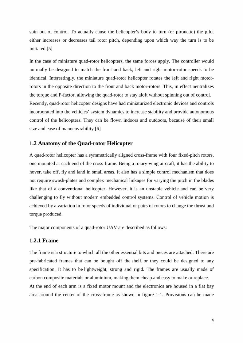
At the end of each arm is a fixed motor mount and the electronics are housed in a flat bay
area around the center of the cross-frame as shown in figure 1-1. Provisions can be made
5
underneath the frame for a payload such a camera or a robotic arm, depending on the mission
to be accomplished by the quad-rotor.
Figure 1-1: Quad-rotor helicopter frame
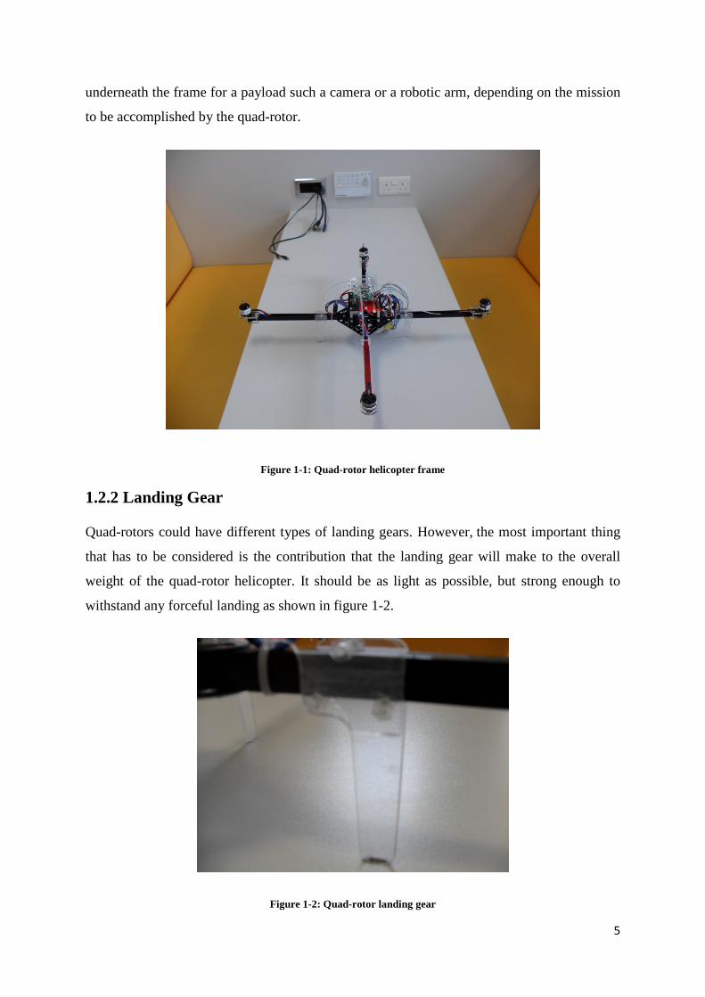
1.2.2 Landing Gear
Quad-rotors could have different types of landing gears. However, the most important thing
that has to be considered is the contribution that the landing gear will make to the overall
weight of the quad-rotor helicopter. It should be as light as possible, but strong enough to
withstand any forceful landing as shown in figure 1-2.
Figure 1-2: Quad-rotor landing gear

6
1.2.3 Motors and Propellers
The Quad Rotor’s actuation mechanisms are relatively simple as shown in figure 1-3. The
Quad Rotor uses four brushless motors to power the propellers. Brushless Motors generate
more power, have greater efficiency, are more reliable, produce less noise and a longer
lifetime than brushed motors. However, they are obtained at a higher cost. Each of the four
brushless motors is independently controlled by an electronic speed controller (ESC). An
ESC takes input from a logic board and sends varying pulses to the motor to make it spin at
different rates.
The propellers are used to provide the thrust for lifting and maneuvering the quad-rotor and
each is directly attached to a brushless motor. The size of the propeller is important as it
directly affects power consumption and lift generation.
Figure 1-3: Propeller mounted on a brushless DC motor
The motors and propellers are configured such that two of them spin clockwise and other two
spin counter-clockwise. This arrangement brings about a balance of forces and moments,
giving some stability to the quad-rotor helicopter.
1.2.4 Battery
Quad-rotor helicopters are known for high energy consumption as a major drawback. They
are normally fitted with lightweight rechargeable batteries that have the capacity to power the
motors and other electronics through the desired flight endurance period. Most quad-rotor
helicopter manufacturers use Lithium-ion Polymer (LiPoly) batteries as shown in figure 1-4.

7
Figure 1-4: Battery
1.2.5 Sensors
Quad-rotors are equipped with flight sensors, including – accelerometers, gyroscopes, sonars,
barometric pressure sensors and GPS receivers as shown in figure 1-5. Sensors are very
important as they can help any robotic device in understanding its environment by estimating
the state of the robot. Data obtained from sensors can tell if the vehicle is going to flip over
when it tilts one more degree; if it is flying horizontally or if it is nose-diving, if there are
other vehicles or objects within range.
All of these sensors are continually sending their outputs to an on-board flight computer.
These signals are then analysed, processed and adjustments made to keep the helicopter aloft.
Figure 1-5: Inertial measurement unit

8
a) Accelerometer
An accelerometer is an electromechanical device that measures forces due to acceleration.
These forces may be static – like the gravitational pull or they could be dynamic – as a result
of movements or vibrations.
The angle of tilt of the vehicle with respect to the earth can be determined by measuring the
amount of static acceleration due to the gravitational pull. Furthermore, analysis of the
movement of the device can be done by sensing the amount of dynamic acceleration.
b) Gyroscope
A gyroscope is a device for measuring or maintaining orientation of the vehicle, based on the
principle of conservation of angular momentum. It measures angular velocity by detecting
Coriolis acceleration and is typically used for measuring the rate of rotation of the vehicle.
Conventional aircrafts would normally use about a dozen gyroscopes in everything from its
compass to its autopilot.
An arrangement of three sensitive accelerometers and two gyroscopes, with their axes lined
up at right angles on the quad-rotor helicopter structure articulates accurately where the
vehicle is heading. It also tells how its motion is changing in all three directions.
c) Sonar
A sonar sensor is a device that is designed to use sound propagation to detect obstacles in the
robot’s environment. It creates a pulse of sound and then listens for reflections of the pulse.
To measure the distance from the transmitter to an object, the time broadcast of a pulse to
reception is measured and converted into a range by knowing the speed of sound.
d) Barometric pressure sensor
A barometric pressure sensor usually acts as a transducer and generates an electrical signal as
a function of the pressure imposed. It is often used for monitoring and control in numerous
applications. To sustain its altitude, a quad-rotor helicopter requires such a transducer.
e) GPS receiver
This sensor uses the Global Positioning System, a satellite-based navigation system that
sends and receives radio signals. It provides information about current location in different
weather conditions in an unobstructed line of sight to four or more GPS satellites. The
accuracy of the GPS signal may vary from a few meters to a hundred meters, depending on
its configuration.

9
1.2.6 Flight Control Board
The flight control board is a critical element of the quad-rotor helicopter, as it essentially acts
as the brains of the vehicle. It houses the sensors (accelerometers, gyroscopes and barometric
pressure sensor) as shown in figure 1-6.
Since quad-rotors don't glide like the fixed-wing aircrafts, the only thing that keeps them aloft
is the precise control of the motors and propellers. The flight control board uses the sensors to
keep track of the vehicle’s position and orientation by monitoring how the quad-rotor flies in
relation to its environment and the commands given to it.
Figure 1-6: Flight control board
1.2.7 Transmitter and Receiver
These are the parts that send and receive signals between the quad-rotor and the remote
control or ground station. The transmitters and receivers (pictured in figure 1-7) are also very
important in communication between vehicles when a swarm of quad-rotors are working
together cooperatively.
There is a wide range of receiver and transmitter combination; however, most quad-rotor
helicopters use the traditional remote controls and radio frequency technology.
10
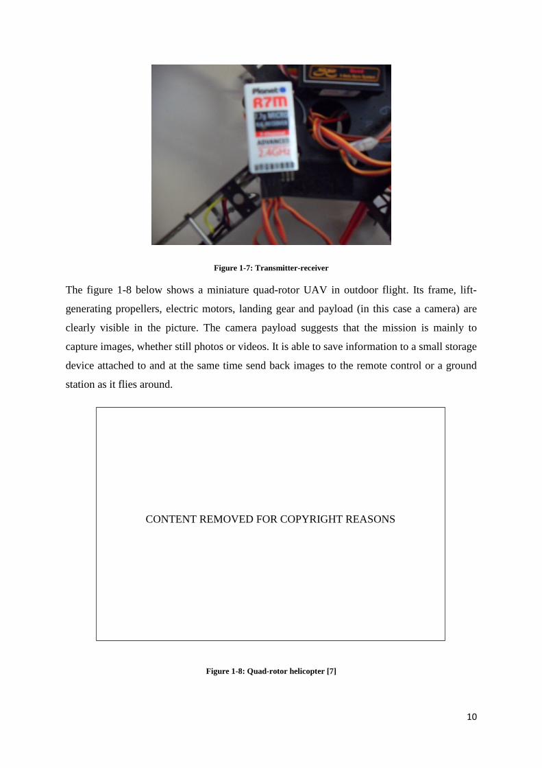
Figure 1-7: Transmitter-receiver
The figure 1-8 below shows a miniature quad-rotor UAV in outdoor flight. Its frame, lift-
generating propellers, electric motors, landing gear and payload (in this case a camera) are
clearly visible in the picture. The camera payload suggests that the mission is mainly to
capture images, whether still photos or videos. It is able to save information to a small storage
device attached to and at the same time send back images to the remote control or a ground
station as it flies around.
Figure 1-8: Quad-rotor helicopter [7]
CONTENT REMOVED FOR COPYRIGHT REASONS

11
1.3 Basic concepts of the quad-rotor helicopter
The quad-rotor helicopter is very well modelled with its four rotors in a cross configuration
style. Two of the motors (front-1 and rear-3) rotate counter-clockwise, while the other two
(left-2 and right-4) rotate clockwise. In this configuration, the helicopter does not spin on its
vertical axis since the rotational inertia is cancelled out, completely eliminating the need for a
tail rotor which is used to stabilize the conventional helicopter. When the pair that's spinning
in one direction is faster than the other pair, the helicopter will spin on its vertical axis,
thereby leading to a change of heading or control of the helicopter’s direction of movement.
Angular accelerations about the pitch and roll axes can be caused separately without affecting
the yaw axis. Each pair of blades rotating in the same direction controls one axis, either roll
or pitch, and increasing thrust for one rotor while decreasing thrust for the other will maintain
the torque balance needed for yaw stability and induce a net torque about the roll or pitch
axes. This way, fixed rotor blades can be made to manoeuvre the quad-rotor vehicle in all
dimensions. Translational acceleration is achieved by maintaining a non-zero pitch or roll
angle.
The figure 1-9 below shows a simplified quad-rotor helicopter structure in hover state, with
the red circle defining the front of the vehicle.
Figure 1-9: Simplified quad-rotor helicopter structure
Hovering is the term used to describe a situation when a helicopter maintains a constant
position at a selected point in the air. At this point, it can be said that the forces of lift and
weight have reached a state of equilibrium. Generally, helicopters can climb or descend by
upsetting the vertical balance of forces acting on them.

12
In figure 1-9 above, all the propellers rotate at the same (hovering) speed to generate a
collective lift force that offsets the weight of the quad-rotor helicopter (which equals its mass
multiplied by acceleration due to gravity acting at the centre of the cross frame of the
vehicle). Consequently, the quad-rotor neither climbs nor descends, it does not stall, roll,
pitch or yaw and therefore there is no horizontal movement in any direction. It stays at a fixed
point in the air and does not move from its position because there is a balance in all the forces
and torques that are acting on the vehicle.
Despite its six degrees of freedom (DOF), the quad-rotor helicopter is equipped with only
four propellers. Therefore it is not possible to reach a desired set-point for all the DOF, but
four at a maximum. Nevertheless, because of its structure, it is possible to choose the four
best variables that can be controlled and to decouple them, thereby making the controller
formulation a lot easier. The four quad-rotor targets are related to four basic control actions,
which allow the vehicle to reach a certain altitude and attitude. These control actions are
described as follows:
1.3.1 Throttle
This control action is realized by simultaneously increasing (or decreasing) all propeller
speeds by identical amounts as shown in figure 1-10. In consequence, the quad-rotor
helicopter is raised or lowered to a certain altitude, because of the collective vertical force
generated by the four propellers with respect to the body-fixed frame. It is expected that if the
helicopter is in horizontal position, the vertical direction of the inertial frame and that of the
body-fixed frame should coincide. Otherwise the provided thrust generates accelerations in
both vertical and horizontal directions in the inertial frame.
Figure 1-10: Throttle command response

13
1.3.2 Roll
The roll command is provided by simultaneously increasing (or decreasing) the left propeller
speed and decreasing (or increasing) the right propeller speed, while keeping the front and
rear propellers spinning at the same speed. With one rotor spinning faster than the rotor on
the opposite side, more lift will be generated on the side of the faster spinning rotor, thereby
tilting the helicopter to the opposite side. This is because of the torque created by the changes
in lift forces with respect to the quad-rotor body x-axis and that creates a roll angle, φ, as
shown in figure 1-11.
When the helicopter is tilted, the air is deflected slightly sideways instead of directly
downwards, and the helicopter will move in the direction of its tilt. The total vertical thrust is
maintained as in hovering, thus this command leads only to a roll angular acceleration.
Figure 1-11: Roll command response
1.3.3 Pitch
The pitch and roll commands are very similar. It is provided by simultaneously increasing (or
decreasing) the rear propeller speed and decreasing (or increasing) the front propeller speed,
while keeping the left and right propellers spinning at the same speed. Since more lift is
generated on the side of the faster spinning rotor, the helicopter will tilt towards the side of
the slower spinning rotor. This is because of the torque created by the changes in lift forces
with respect to the quad-rotor body y-axis and that creates a pitch angle, θ (known as a nose-
up or nose-down in a conventional aircraft), as shown in figure 1-12.
When the helicopter is tilted, the air is deflected slightly sideways instead of directly
downwards, and the helicopter will move in the direction of its tilt. Again, the total vertical
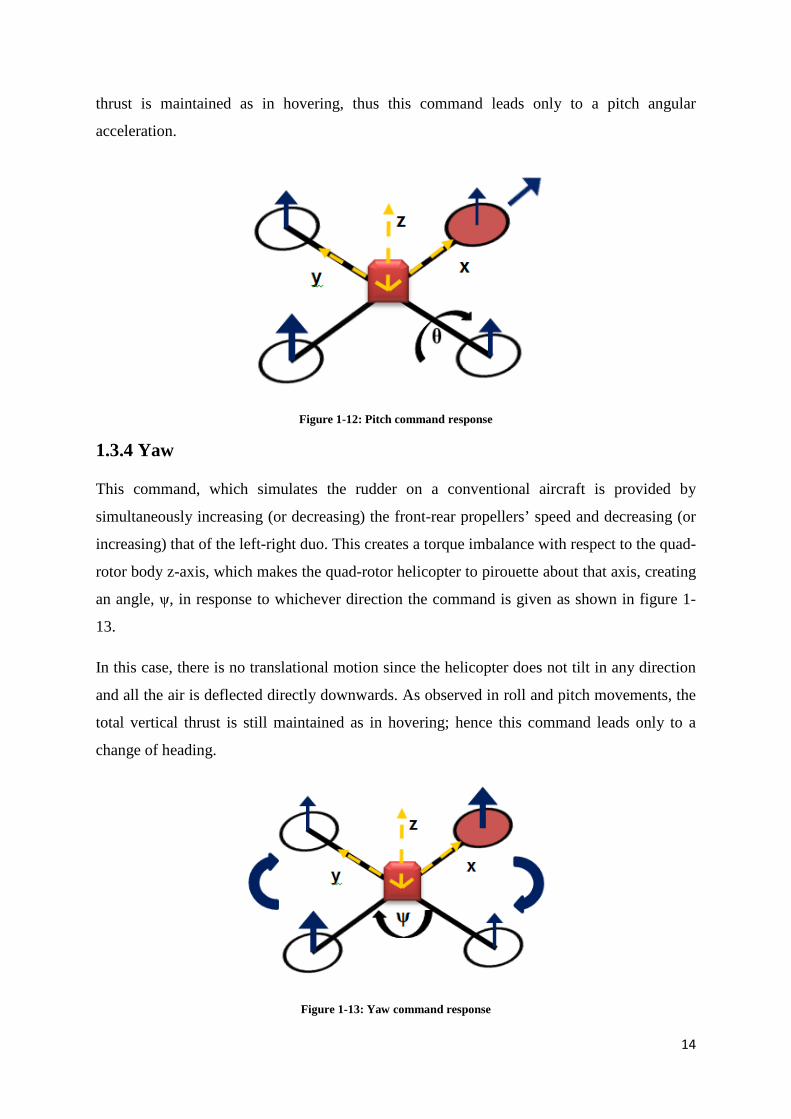
14
thrust is maintained as in hovering, thus this command leads only to a pitch angular
acceleration.
Figure 1-12: Pitch command response
1.3.4 Yaw
This command, which simulates the rudder on a conventional aircraft is provided by
simultaneously increasing (or decreasing) the front-rear propellers’ speed and decreasing (or
increasing) that of the left-right duo. This creates a torque imbalance with respect to the quad-
rotor body z-axis, which makes the quad-rotor helicopter to pirouette about that axis, creating
an angle, ψ, in response to whichever direction the command is given as shown in figure 1-
13.
In this case, there is no translational motion since the helicopter does not tilt in any direction
and all the air is deflected directly downwards. As observed in roll and pitch movements, the
total vertical thrust is still maintained as in hovering; hence this command leads only to a
change of heading.
Figure 1-13: Yaw command response

15
1.4 Applications of Miniature Quad-rotor Helicopters
Modern society is no longer tolerant to the losses of human lives. Regardless of whether these
losses emanate from a war or a hazardous accident; the mind-set of the global citizen cannot
simply accept death in such a technically advanced world. The aviation industry, since
inception has witnessed the loss of human lives as a result of accidents; and however much of
funding and devotion the industry commits in order to provide safety will not prevent such
mishaps from happening. It is very improbable, even in the future that such mishaps will be
completely eradicated, since factors such as human error and dangerous flight situations are
beyond human control.
The removal of the pilot from the cockpit gives UAVs a great advantage over manned
aircraft, such that at no time during flight are human lives at stake. This advantage gives them
the ability to carry out operations, which their manned counterparts find very tasking and
dangerous to do. Some of the many examples of missions that could be classified as unsafe
for manned aircrafts are – surveillance over nuclear reactors, surveillance over hazardous
chemicals, fire patrol, volcano patrol, hurricane observations and rescue missions over
adverse weather conditions [8].
The unsuitability of manned aircraft in undertaking these types of missions has repeatedly
occurred throughout history. There have been situations where survivors from sea accidents
were drowned, just because the aerial rescue operation conducted by manned aircraft was
delayed in tracking them due to bad weather, which the pilots had to contend with. In the
past, UAVs have been given the chance to test their capabilities in executing operations that
were considered too risky for manned aircrafts. A good example is the Aerosonde UAV,
which was flown around the tropical cyclone Typhoon in the western coast of Australia in
1998. The mission was a great success as it turned out to be the very first time when
meteorologists were able to take readings from an aerial platform so close to the cyclone [9].
Miniature quad-rotor helicopters have extremely varying application domains that cover
many indoor and outdoor applications including:
1.4.1 Border Patrol
Miniature quad-rotor helicopters have been engaged in aerial surveillance and monitoring of
borders, ground based objects. With intelligent computer control and minimal human
supervision, individual or multiple autonomous quad-rotors are able to patrol borders. The

16
use of a swarm of quad-rotors would permit continuous aerial surveillance, with new vehicles
launched to take over from those in need of a battery recharge or ones that may have been
damaged in the process [10].
Many countries and organizations are making efforts in wildlife conservation to protect rare
and endangered animals like the one-horned rhino from poachers by using such UAVs to
patrol the borders of the vast parks as shown in figure 1-14. This is made possible because
multiple and distributed quad-rotor platforms working together can create the potential for a
dynamic wireless routing layer, where the increased throughput and extended range of a mesh
network becomes very beneficial.
Figure 1-14: An image from a UAV on border patrol [11]
1.4.2 Disaster Management/ Search and Rescue
There have been a large number of natural and man-made disasters throughout the world.
Some of them are due to earthquakes, weather conditions or human acts of terrorism (e.g. the
World Trade Centre Twin Tower attacks – 2001, Hurricane Katrina – 2005, the Haiti
earthquake – 2010, the Japanese earthquake and tsunami – 2011, the Nairobi mall siege –
2013 among others). In such situations, disaster management or search and rescue teams have
to swing into action to contain a situation or to find and save the victims as shown in figure 1-
15.
CONTENT REMOVED FOR COPYRIGHT REASONS
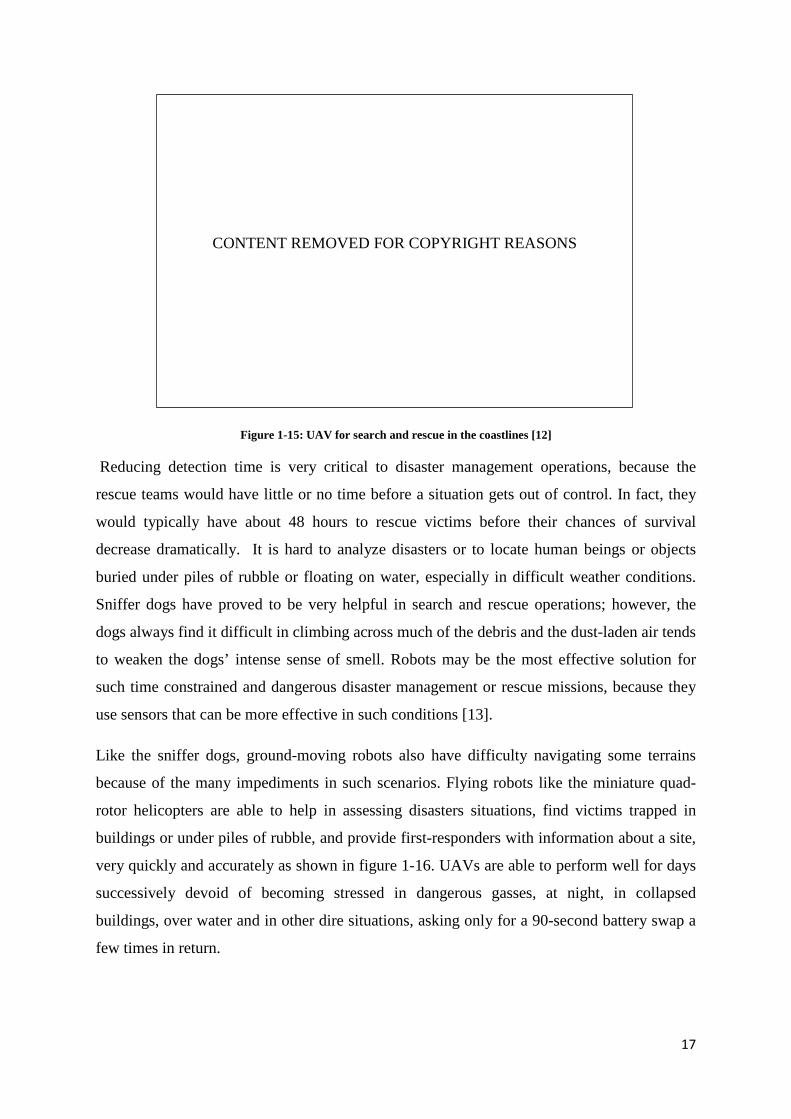
17
Figure 1-15: UAV for search and rescue in the coastlines [12]
Reducing detection time is very critical to disaster management operations, because the
rescue teams would have little or no time before a situation gets out of control. In fact, they
would typically have about 48 hours to rescue victims before their chances of survival
decrease dramatically. It is hard to analyze disasters or to locate human beings or objects
buried under piles of rubble or floating on water, especially in difficult weather conditions.
Sniffer dogs have proved to be very helpful in search and rescue operations; however, the
dogs always find it difficult in climbing across much of the debris and the dust-laden air tends
to weaken the dogs’ intense sense of smell. Robots may be the most effective solution for
such time constrained and dangerous disaster management or rescue missions, because they
use sensors that can be more effective in such conditions [13].
Like the sniffer dogs, ground-moving robots also have difficulty navigating some terrains
because of the many impediments in such scenarios. Flying robots like the miniature quad-
rotor helicopters are able to help in assessing disasters situations, find victims trapped in
buildings or under piles of rubble, and provide first-responders with information about a site,
very quickly and accurately as shown in figure 1-16. UAVs are able to perform well for days
successively devoid of becoming stressed in dangerous gasses, at night, in collapsed
buildings, over water and in other dire situations, asking only for a 90-second battery swap a
few times in return.
CONTENT REMOVED FOR COPYRIGHT REASONS

18
Figure 1-16: UAV for search and rescue in disaster situations in the Philippines [14]
1.4.3 Wild fire detection
UAVs equipped with advanced infrared sensors can perform surveillance and fire detection
missions over forests (where access by foot or ground vehicles is difficult or impossible) and
alert the fire brigade on time. Wildfires differ from other fires by their extensive sizes, the
speed at which they can spread, their potential to change direction unexpectedly, and their
ability to jump gaps such as roads, rivers and fire breaks. In many parts of the world, they
pose a great risk to life and infrastructure as they can have negative ecological effects and
cause extensive damage to human lives and property [15].
Early detection is a key factor to wildfire fighting. Strategies of wildfire prevention, detection
and suppression have varied over the years – including public hotlines, fire lookout towers
and ground patrols. However, the accuracy of these methods, which largely depend on human
observations have their limitations such as operator fatigue, time of the day, time of the year
and geographic location. As captured in figure 1-17, aerial monitoring through the use of
quad-rotor helicopters can provide a wider view and give more accurate information about
the location of the outbreak of the fire as well as many other factors, which could aid the
spread of the fire – such as wind speed, temperature and humidity [16].
CONTENT REMOVED FOR COPYRIGHT REASONS

19
Figure 1-17: Fire monitoring using a UAV (left) and a thermal infrared scanner (right) [16, 11]
1.4.4 Photography
The field of aerial imagery has seen the largest use of miniature quad-rotor helicopters. Such
vehicles have within very short periods of time helped photographers create 3-dimensional
models of many locations instead of the normal flat maps. Having on-board cameras gives
the users the option of streaming live videos to the ground when the helicopter is aloft.
Several establishments have also used this for real estate photography and property inspection
as shown in figure 1-18. Others take advantage of the quad-rotor’s closed-circuit television
capabilities and ability to provide an eye in the sky to the action below.
Figure 1-18: Remote controlled helicopters fitted with cameras fly above Sydney [17]
CONTENT REMOVED FOR COPYRIGHT REASONS
CONTENT REMOVED FOR COPYRIGHT REASONS

20
1.4.5 Military and Law enforcement
UAVs can take on the role of manned police helicopters in a more cost effective way as they
can quietly hover when stalking or collecting status data of an object of interest and beam
back information or images to the military and law enforcement agencies as shown in figure
1-19. Their small size enables them to penetrate an enemy's radar defences because of their
decreased radar, acoustical and infrared signatures. This prevents them from being easily
detected by the enemy. Even if they are detected and shot down, no human life would be lost
as the operator would not be on-board like that of a manned aircraft [8].
These vehicles could serve as mobile communication links between military commands
where or when satellite or radio communication installations are unavailable. They could also
be configured and deployed as a swarm of vehicles to form a co-operative structure, forming
a dynamic communication network that reconfigures itself based on needs or circumstances
leading to constant communication coverage of the combat area. A real time view of the
combat area will be very helpful to commanders in making quick and tactical real time
decisions that could lead to victory.
Figure 1-19: UAVs assist the law enforcement agencies with tracking and aerial photography [11]
1.4.6 Research
Any kind of research (environmental, atmospheric, archaeological, pollution and many more)
can be carried out by UAVs equipped with the appropriate payloads. Miniature quad-rotor
helicopters are popular devices that are used by universities and research establishments in
CONTENT REMOVED FOR COPYRIGHT REASONS

21
testing and assessing innovative concepts and designs in a number of diverse fields as shown
in figure 1-20.
They are relatively cheap to acquire, available in a range of shapes, sizes and configurations,
with their simple mechanical design meaning not much of maintenance is required. Due to
the multi-disciplinary nature of quad-rotors, researchers from a number of fields need to align
their skills and efforts to make momentous improvements to the way quad-rotors perform.
Such research projects are characteristically partnerships between aerospace engineering,
control engineering, mechanical engineering, electrical engineering, artificial intelligence and
computer science experts.
Major world-class research laboratories currently working on advanced control techniques
and applications for quad-rotors are MIT's Aerospace Controls Lab, ETH's Flying Machine
Arena, University of Essex Robot Arena, STARMAC at Stanford University and GRASP
Lab at University of Pennsylvania [18].
Figure 1-20: Flight demo at University of Derby (left) and the autonomous squadron from KMel Robotics (right) [19]
1.4.7 Agricultural and Industrial applications
When it comes to agricultural and industrial applications, quad-rotors have proved to be very
useful. Such applications can be crops spraying, nuclear factory surveillance, surveillance of
pipelines and many more.
Farmers are already using miniature quad-rotors to monitor their crops in the field. An
overhead picture of a farm taken at regular intervals can give information needed to adjust the
CONTENT REMOVED FOR COPYRIGHT REASONS
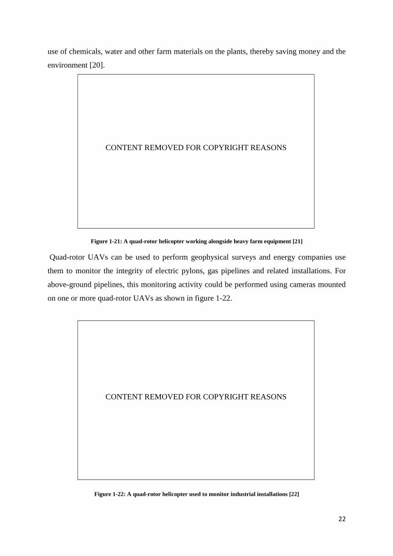
22
use of chemicals, water and other farm materials on the plants, thereby saving money and the
environment [20].
Figure 1-21: A quad-rotor helicopter working alongside heavy farm equipment [21]
Quad-rotor UAVs can be used to perform geophysical surveys and energy companies use
them to monitor the integrity of electric pylons, gas pipelines and related installations. For
above-ground pipelines, this monitoring activity could be performed using cameras mounted
on one or more quad-rotor UAVs as shown in figure 1-22.
Figure 1-22: A quad-rotor helicopter used to monitor industrial installations [22]
CONTENT REMOVED FOR COPYRIGHT REASONS
CONTENT REMOVED FOR COPYRIGHT REASONS

23
1.5 Chapter Summary
Over the past two decades, the research community has taken particular interest in UAVs
because of the emergence of a large number of potential civil and military applications.
Currently, many research establishments are working to produce remotely piloted UAVs that
are capable of air to air combat, aerial refueling, combat search and rescue with facial
recognition, resupply to agents on the ground and many more.
The possibilities of the use of such vehicles are endless, because in future, they will be able to
perform an increasingly sophisticated array of missions apart from what they are capable of
doing today. However, such vehicles will never fully replace humans because of the costs
involved in developing systems as complicated as humans and technical risks that would
follow the implementation of such systems.
24
CHAPTER 2
STATE OF THE ART AND KEY RESEARCH REVIEWS
This chapter provides a review of literature, which is relevant to the study and which
critically appraises the works of others. It goes on to outline the state of the art principles of
control and simulation techniques as applied in this research, giving examples of their general
applications in problem solving and specifically stating their applications relating to flight
control – namely Computational Fluid Dynamics (CFD), Artificial Neural Networks (ANNs)
and Fuzzy logic (FL). It also provides the background for the research with details of the
project aim and objectives; gives a justification for the choice of control technique and
highlights the contributions of this work.
25
2.0 Previous works on the quad-rotor helicopter
UAVs have continued to capture enormous commercial potential by attracting the attention of
many people including laymen, potential appliers, vehicle professionals and researchers.
Research and development in this field has gained increasing significance, due to the
emergence of a large number of potential civil applications. Several structures and
configurations have been developed to allow 3-D movements. For example, there are blimps,
fixed-wing planes, single rotor helicopters, bird-like prototypes, quad-rotors, etc. Each of
them best suited for certain types of missions, considering their advantages and drawbacks.
A plethora of research groups are using the quad-rotor design as a test bed for a
swarm of projects. Some of the common uses are in developing advanced control systems,
improved autonomous control, sensor arrays and surveillance equipment. To effectively
control the quad-rotor helicopter, two major motion problems have to be carefully analysed
and solved. First, it should be able to hover stably and second, it should be able to keep up
with the planned path and speed, despite any disturbance.
With the rapid advancement in electronics leading to the availability of miniaturized motion
sensors, high power to weight ratio batteries and high speed DC motors, there have been
many different approaches to the control of quad-rotors; none of which may either be
completely right or wrong, because the solutions to these problems are not straight forward.
Some are obviously more suited than others in some situations, but any working alternative
can be defended.
The numerous amount of published work using quad-rotor design is suggestive of the variety
of topics involved. While the bulk of the published work deals with control systems and
sensor arrays, some papers have dwelt on developing accurate aerodynamic models,
improving the system design and developing point-to-point real time communication between
multiple quad-rotor vehicles. The hobbyist community has not been left behind as it has
documented a great deal of work with regards to developing very cheap home built (possibly
DIY) quad-rotors for personal use.
There have been a number of attempts to build quad-rotors, by and large though; the
dynamics for all the different models remain unchanged [23]. There are a few exceptions,
however, such as Dodd in [24] made provision for the rotors to be tilted to achieve
translational motion without necessarily rotating the vehicle. Researchers use the quad-rotor

26
helicopter as an excellent test-bed for advanced control techniques due to the simplicity of
their construction and maintenance, their ability to hover and also to take-off and land
vertically and also the fact that control of the vehicle is achieved only by varying the speed of
the 4 rotors.
A notable group that has contributed to quad-rotor literature is Castillo et al [25], whose work
has looked into back-stepping with nested saturations, for real-time control of the quad-rotor.
This non-linear control technique has constraints placed on the amplitudes of the inputs; it
then operates to meet these constraints. It seemed to perform well in the presence of
disturbances. In [26], the same group compared the nested saturation approach with classical
PD control, where the benefits of the nested saturations algorithms are shown to be an
improved handling of disturbances.
Bouabdallah [27], developed PID controllers for orientation stabilization and modern LQ
control are compared, despite realizing that the later one yielded average results due to
assumptions made during modelling that could have introduced errors into the control
strategy. The main advantage of this technique is that the optimal input signal turns out to be
obtainable from full state feedback (by solving the Ricatti equation). On the other hand the
analytical solution to the Ricatti equation is difficult and takes time to compute. The OS4
Project was started at the Swiss Federal Institute of Technology in 2003 with an aim to
develop devices for searching and monitoring hostile indoor environments. It resulted in the
development of a control law based on classical control and also modern control
methodology.
Over the years, the Australian National University has carried out meticulous studies on
quad-rotors. The X4-flyer Mark II, which weighs about 2kg and measures up to 70cm in
length with rotors of 11inch diameter, was designed and fabricated [23]. They incorporated a
discrete-time PID control law to their model, including the very fast blade flapping dynamics.
The closed loop behaviour turned out to be poor at higher speeds, approaching an unstable
behaviour and that was attributed to high-frequency noise from the rotors interfering with the
accelerometer readings.
The Robotics Laboratory of Versailles [28, 29, 30] has also considered sliding mode control,
back stepping and dynamic feedback for stabilization and simple trajectory tracking. Here,
the dynamic feedback control was implemented on quad-rotor test beds to transform the
closed loop part of the system into a linear, controllable and decoupled subsystem but was

27
seen to be insufficient to cope with significant external disturbances, the sliding mode
controller proved to be better in simulation.
Tayebi and McGilvary in [31, 32] undertook a thorough study on control techniques for
attitude stabilization of a quad-rotor. They used quaternion for attitude representation,
Lyapunov stability criterion and a PD2 feedback structure, with which a model-independent
PD controller was compared. Both configurations achieved stability and disturbance
rejection. Their experimental results start a deviation from the trend within the papers
reviewed that seems to suggest that traditional linear controllers are not sufficient for
stabilization of the quad-rotor.
Other examples of trajectory following controllers include [33], where H∞ is considered. This
control technique, using a two degree of freedom architecture has the ability to cope with
modelling inaccuracies. The results through simulation show good tracking as well as good
disturbance rejection. In [34], Driessen and Robin proposed a two phase controller in which
the first phase considers attitude and the second phase position and the yaw angle. Using
differential flatness, global convergence of the tracking error to zero is proven assuming
positive thrust.
There are considerably fewer trajectory generation papers for the quad-rotor. In [35] output
space trajectory generation is considered using differential flatness. Here, they only consider
straight line trajectories using a simple parameterization and is, therefore, not considering
optimality and is assuming feasibility of the straight line.
The fluctuation and/or unavailability of GPS signals inside buildings or in certain areas with
high rise buildings or mountains creates a situation where the papers reviewed so far are
usually based on simulation results with a number also including results from a 2 degree of
freedom experimental rig. There are a number of alternatives for solving this problem. In [36]
the test-bed at Massachusetts Institute of Technology (MIT) is described. Consisting of
VICON cameras and a number of quad-rotors with visual markers, this system provides
accurate attitude and position feedback to a ground station; however, the system is certainly
not cheap and does not offer a commercial solution.
At Stanford University a multiple vehicle test-bed is used for comparison of design control
techniques [37]. This test-bed with a capacity for up to 8 vehicles [38] is only operational
outdoors however as it relies on GPS. A cheaper solution which has been considered by a

28
number of institutions is that of visual feedback. In [39] and [40] two cameras are used for
POSE (Position and Orientation) estimation, one camera is on-board the vehicle and the
second is a ground based pan tilt camera. This set up is used to compare nonlinear control
techniques. However this is not a complete solution as noted in [39] ‘A helicopter cannot be
fully autonomous if it depends on an external camera.’ In [41] a single on-board camera
system is proposed which tracks a moving ground vehicle. In [42] a circular trajectory is
followed, using a positional estimate, obtained through an on-board camera, viewing a square
target on the ground.
In [43] an adaptive neural network control to stabilize a quad-rotor helicopter against
modelling error and wind disturbance was proposed. It was compared with both dead zone
and e-modification adaptive techniques, but also stops at a simulation without
implementation on the real hardware. The results of the simulation show an improvement in
achieving a desired attitude and reduction of weight drift.
In [44], the group tried to augment a conventional PD controller conceived mainly for
hovering, with an adaptive element using a real-time tuning single hidden layer neural
network in an inner-outer loop combined architecture to account for model inversion error
cancellation, issued in the feedback linearization process. Simulation results show a good
performance of the augmented controller in tracking manoeuvres.
In [45] the quad-rotor’s linearized equations of motion were used to develop control laws for
way point tracking paths. The performance of the laws with uncertainties such as wind and
saturation were analysed and results showed that the laws do not perform well when there is
an uncertainty. In [46], system modelling and control algorithm development was done, with
a comparison of PID controllers developed. A simulator and a real platform were developed
to test the results.
AI-Younes and Jarrah [47] introduced a backstepping fuzzy Logic controller (BFL) and
backstepping least mean square controller (BLMS) as new approaches to control the attitude
stabilization of a quad-rotor. A recursive Lyapunov function was used bring about stability
around a fixed set-point using backstepping control algorithm. The BFL controller utilizes the
advantage of fuzzy logic to schedule the backstepping controller parameters. It showed
improved performance compared with that achieved by backstepping controller alone. A
comparison between Backstepping, BFL and BLMS controllers showed that the BLMS
29
controller suffered from a slow time response while having reduced control effort when
compared with the BFL controller.
Abeywardena [48] used a fuzzy logic design to try to stabilize and control the quad rotor. The
controller was controller was then used to achieve stable hovering of the quad-rotor, amidst
velocity disturbances. The simulation results show good results at stable hover.
Dierks [49] introduced a framework for leader-follower formation control for multiple quad-
rotor UAVs, based on spherical coordinates. The control objective for the follower UAV is to
track its leader at a desired- separation, angle of incidence, and a bearing by using an
auxiliary velocity control. Then, a neural network (NN) control law for the dynamical system
was introduced to learn the complete dynamics of the UAV including unmodelled dynamics
like aerodynamic friction. Results show some stability achieved in the entire formation using
Lyapunov theory.
Raffo [50] used dynamic motion equations obtained by Lagrange-Euler formalism in a
hierarchical control structure consisting of a model predictive controller (MPC) to track the
reference trajectory together with a non-linear H∞ controller to stabilize the rational
movements. The trajectory was maintained by performing an on-line trajectory re-
optimization during the flight to obtain the optimal path in terms of cost. This makes it adapt
to the constantly changing environment. In both controllers, the integral of the position error
was considered and a null steady-state error was achieved when sustained disturbances acted
on the system.
Theerasak [51] worked on a control methodology for a UAV with quad-rotor mechanism. A
conventional PID controller and self-tuning PID based on fuzzy logic were compared and
analyzed. The performance results of the two controllers when applied to a quad-rotor UAV
show that both controllers are acceptable in the case of no variation in load.
Again, Pounds [6] used tuned plant dynamics with an on-board embedded attitude controller
to stabilize flight, independent linear SISO controllers were designed to regulate flyer attitude
and performance of the system was demonstrated in indoor and outdoor flight.
Dierks [52] proposed a nonlinear controller for a quad-rotor UAV, using neural networks
(NNs) and output feedback. The NN is introduced to learn the complete dynamics of the
UAV online and an NN observer is introduced to estimate the translational and angular

30
velocities of the UAV, and an output feedback control law is developed. Simulations show
that the proposed controller outperforms a conventional linear controller.
In 2008, He [53] developed a motion planning algorithm for a quad-rotor helicopter flying
autonomously without GPS using the Belief Roadmap (BRM) Algorithm to plan the vehicle
trajectory that incorporates sensing. The helicopter was able to navigate an indoor
environment with a laser range-finder. Cowling [1] achieved trajectory following using a
number of linear control techniques, with the LQR being unable to adapt to environmental
changes. A test of Model-based predictive control (MBPC), was found to guarantee
constraint satisfaction at every time step, but was also found to be time consuming and
therefore a combined controller was proposed using MBPC and LQR.
Balas [54] described the use of PID and LQR methods to control the position and the yaw
angle of a quad-rotor helicopter using a full non-linear Simulink model, starting with the
most mathematical approach and moving towards the most physically feasible approach.
Results show that the quad-rotor was satisfactorily able to track the given input trajectory.
Lee [55] in 2010 developed a nonlinear tracking controller on the special Euclidean group SE
(3) with desirable closed loop properties that are almost global and went on to illustrate the
versatility of the controller in simulations. Markus [56] presented an algorithm that calculates
the flight trajectories for quad-rotors, with a demonstration of the trajectory generation and
tracking performance at the ETH Zurich Flying Machine Arena test-bed. It was observed that
the unmodelled aerodynamic effects caused trajectory deviations when the helicopter was
decelerating from high speeds – with an emphasis on the need for improving the performance
and correcting for aerodynamic effects.
Stingu [57] in 2011, focused on quad-rotor control and heterogenous multi-vehicle
cooperation. In this work, reinforcement learning algorithms were used to design suboptimal
controllers for a class of complex systems that can be conceptually split in local loops with
simpler dynamics and relatively weak coupling to the rest of the system.
In 2012, Mellinger [58] described an approach to modelling and control of a single quad-
rotor, with methods that worked well for near hover flight and also controls for large roll or
pitch angles. The thesis also extended the developed control methods to systems with
multiple quad-rotors attached to the same rigid body, enabling the vehicles to work together
and then went on to develop trajectory generation methods for the vehicles.

31
Javier [59] attempted to prove the viability of using a quad-rotor helicopter as a measurement
instrument of wind profiles within large offshore wind farms. The project analyzed the idea
of wind profile characterization by relating the attitude of a quad-rotor to local wind profile.
In 2013, Kushleyev [60] described a prototype of an autonomous micro quad-rotor with on-
board attitude estimation and control that operates with an external localization system. The
paper went on to discuss the aerodynamics of vertical flight and the contributions of ground
effect to the vehicle performance. It also presented architecture and algorithms to coordinate
a swarm of micro quad-rotors.
Abdolhosseini [61] developed a model predictive control algorithm to control a quad-rotor
helicopter. A model reduction technique was developed to reduce the burden of calculations
in the application of the controller into an airborne platform.
In 2014, Alexis [62] developed a model predictive control strategy for the trajectory tracking
of a quad-rotor helicopter. The dynamics of the quad-rotor were modelled using a hybrid
systems approach, and specifically, a set of piecewise affine (PWA) systems around different
operating points of the translational and rotational motions. Simulations show efficiency of
the controller in trajectory tracking and aerodynamic disturbance attenuation.
A number of other works will be referred to in this thesis as found applicable to the chapters.
2.1 The basics concepts of Computational Fluid Dynamics (CFD)
Computational Fluid Dynamics (CFD) is a branch of fluid mechanics that uses numerical
methods and computer algorithms to solve and analyze problems that involve fluid flows.
This design tool has been developed over the past few decades and will continually be
developed as the understanding of the physical and chemical phenomena underlying CFD
theory improves. In CFD, computers are used to execute the calculations required to simulate
the interaction of fluids (liquids and gases) with surfaces defined by boundary conditions.
Using computers with high-speed processors offers better solutions in analyzing and solving
fluid flow problems. The goals of CFD are to be able to accurately predict fluid flow, heat
transfer and chemical reactions in complex systems, which involve one or all of these
phenomena [63].
Presently, CFD is increasingly being employed by many industries either to reduce
manufacturing design cycles or to provide an insight into existing technologies so that they

32
may be analysed and improved to provide solutions to many problems. Examples of such
industries include medical, aerospace, power generation, process industries, automotive,
chemical engineering and construction as shown in figure 2-1.
Figure 2-1: CFD application in automotive simulation (left) and blood flow in the human body (right) [64, 65]
As a design tool, CFD presently sits behind experimental analysis due to the fact that it does
not produce absolute results. The reason for this is that the numerical methods, which govern
the solutions in a CFD problem, rely on several modelling assumptions that may not have
been validated to a satisfactory level. However, [64, 66] state that CFD presently offers itself
as a powerful design tool and even more so in the future because:
a) Dangerous or expensive trial and error experiments can be simulated and design
parameters observed prior to any physical prototype being constructed;
b) Computers are becoming even more powerful and less expensive, thus allowing larger
CFD simulations to be performed, or more detailed simulations of present CFD
problems;
c) The numerical schemes and physical models that are the building blocks of CFD are
continually improving.
d) If a CFD model can be established yielding accurate results on one particular design,
then the model can be used as a tool of prediction for that design under many different
operating conditions.
CONTENT REMOVED FOR COPYRIGHT REASONS
33
2.1.1 Applications of Computational Fluid Dynamics (CFD) in Aircraft Control
Recent technology has led to aircrafts (especially military jets) that often manoeuvre in
extreme conditions of the flight envelope, characterized by vortical flows and great shock
effects - conditions which can cause flight dynamics and aero elastic instabilities [67].
Evidently, the linearized unsteady aerodynamic models no longer work at these conditions
because the approximations cannot effectively cater for the ever-changing flow conditions.
Presently, computational fluid dynamics (CFD) solutions are considered as the state of the art
in modelling unsteady nonlinear flow physics [68] and such solutions provide timely,
enhanced understanding and prediction of the aerodynamic characteristics of aircrafts as
shown in figure 2-2.
It is well known that unsteady aerodynamic forces and moments not only depend on the
instantaneous states but also on all of the states at times before the current state [69].
Unfortunately, this makes the solution of the aircraft equations of motion an infinite-
dimensional problem, where the current states depend on the evolution of previous states at
infinitely many points in time [70]. In [71-73], it is shown that technological advances have
made it possible to solve this problem by developing a full-order model, based on direct
solution of discretized Reynolds-averaged Navier–Stokes (RANS) equations coupled with the
dynamic equations governing the aircraft motion.
It was thought that an alternative approach to creating the full-order model is to develop a
reduced order model (ROM) that seeks to approximate CFD results by extracting information
from a limited number of full-order simulations as described in [74, 75]. These ROM
techniques have been used extensively for flutter prediction, limit cycle oscillation, and gust-
response modelling as seen in [76], but their applications to aircraft stability and control are
still new [77].
34
Figure 2-2: CFD application in simulation of vortices around aircrafts [77]
Details of the CFD process, which has to do with airflow and turbulence simulations as
applied to this research, are presented in chapter 5 of this thesis.
2.2 The basic concepts of Artificial Neural Networks
An artificial neural network is a computational structure inspired by the study of biological
neural processing. There are many different types of neural networks, from relatively simple
to very complex, just as there are many theories on how biological neural processing works.
It is a powerful data modelling tool that is able to capture and represent complex input/output
relationships [78]. The motivation for the development of neural network technology
stemmed from the desire to develop an artificial system that could perform "intelligent" tasks
similar to those performed by the human brain. Neural networks resemble the human brain in
the following ways:
a) A neural network acquires knowledge through learning.
b) A neural network's knowledge is stored within inter-neuron connection strengths known
as synaptic weights.
The human brain is known to contain about 100 billion nerve cells, or neurons. On the
average, each neuron is connected to other neurons through about 10,000 synapses, though
the actual figures may vary greatly from one neuro-anatomy to the other. The human brain's
network of neurons forms an enormous parallel information processing system. This contrasts
CONTENT REMOVED FOR COPYRIGHT REASONS

35
with conventional computers, in which a single processor executes a single series of
instructions. Against this, consider the time taken for each elementary operation, where
neurons typically operate at a maximum rate of about 100 Hz, while a conventional computer
CPU carries out several hundred million machine level operations per second. Despite being
built with very ‘slow hardware’; the human brain has quite remarkable capabilities [79].
The true power and advantage of neural networks lies in their ability to represent both linear
and non-linear relationships and in their ability to learn these relationships directly from the
data being modelled. Traditional linear models are simply inadequate when it comes to
modelling data that contains non-linear characteristics.
ANNs being non-programmed adaptive information processing systems can autonomously
develop operational capabilities in response to an information environment. They learn from
experience and are able to generalize from previous examples. They can also modify their
behaviour in response to the situations they are faced with, and are ideal in cases where the
required mapping algorithm is not known and tolerance to faulty input information is
required. ANNs offer certain advantages over conventional electronic processing techniques.
These advantages are the generalization capability, parallelism, distributed memory,
redundancy, and learning [80].
Figure 2-3 shows a simple artificial neural network model, normally referred to as an MLP
(Multi-Layer Perceptron).
Figure 2-3: Artificial neural network model
Despite ANNs’ attempts to bring computers closer to the human brain's capabilities by
imitating certain aspects of its information processing in a highly simplified way, the
performance of the best ANN is trivial when compared with even the simplest biological
36
system. Artificial Neural Networks are not universal solutions to all problems; they are just
an excellent alternative mathematical device for rapidly processing information and data.
ANNs are being applied to a wide variety of automation problems including adaptive control,
optimization, medical diagnosis, decision making, as well as information and signal
processing, including speech processing. They have proven to be very suitable for processing
sensor data, in particular, feature extraction and automated recognition of signals and multi-
dimensional objects. Pattern recognition has, however, emerged as a major application
because the network structure is suited to tasks that biological systems perform well, and
pattern recognition is a good example where biological systems out-perform traditional rule-
based artificial intelligence approaches.
2.2.1 Applications of Artificial Neural Networks in Aircraft Control
Intelligent flight control systems are the next generation of flight control systems, designed to
provide increased safety for the crew and passengers of aircraft as well as to optimize the
aircraft performance. In the past few decades, major advances have been made in the area of
adaptive control of linear time-invariant plants with unknown parameters. The choice of the
controller structure is normally based on well-established results in the theory of linear
systems, while stable adaptive laws which assure the global stability of the overall system are
derived based on properties of the system to be controlled. Artificial Neural Network based
control schemes have attracted much attention because of their powerful ability to
approximate continuous nonlinear functions as depicted in figure 2-4.
Neural control strategies can be broadly classified into off-line and on-line schemes based on
how the parameters of the network are tuned. When the neural controller operates in an on-
line mode, it has no a priori knowledge of the dynamics of the system to be controlled and the
network parameters are updated while the input – output data is received. In the off-line
control, the network’s parameters are determined from the unknown training pairs and then
those parameters are fixed for control purposes [81]. A neural controller with on-line learning
capabilities can adapt to changes in the dynamics of any system and hence is an ideal choice
for controlling highly nonlinear systems with high degrees of uncertainty [82]. The control
engineering community has continually explored the use of biologically inspired techniques
to solve difficult optimization and control problems [83].
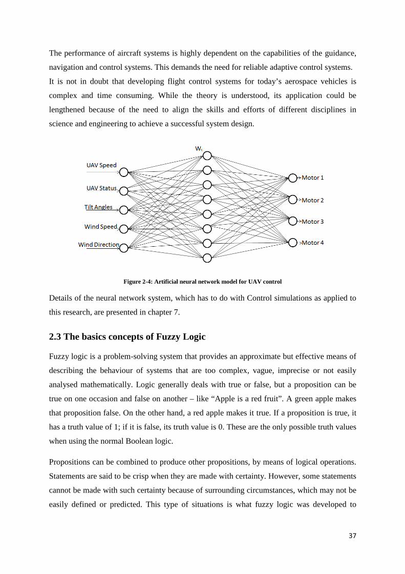
37
The performance of aircraft systems is highly dependent on the capabilities of the guidance,
navigation and control systems. This demands the need for reliable adaptive control systems.
It is not in doubt that developing flight control systems for today’s aerospace vehicles is
complex and time consuming. While the theory is understood, its application could be
lengthened because of the need to align the skills and efforts of different disciplines in
science and engineering to achieve a successful system design.
Figure 2-4: Artificial neural network model for UAV control
Details of the neural network system, which has to do with Control simulations as applied to
this research, are presented in chapter 7.
2.3 The basics concepts of Fuzzy Logic
Fuzzy logic is a problem-solving system that provides an approximate but effective means of
describing the behaviour of systems that are too complex, vague, imprecise or not easily
analysed mathematically. Logic generally deals with true or false, but a proposition can be
true on one occasion and false on another – like “Apple is a red fruit”. A green apple makes
that proposition false. On the other hand, a red apple makes it true. If a proposition is true, it
has a truth value of 1; if it is false, its truth value is 0. These are the only possible truth values
when using the normal Boolean logic.
Propositions can be combined to produce other propositions, by means of logical operations.
Statements are said to be crisp when they are made with certainty. However, some statements
cannot be made with such certainty because of surrounding circumstances, which may not be
easily defined or predicted. This type of situations is what fuzzy logic was developed to

38
model. Fuzzy logic deals with propositions that can be true to a certain degree – somewhere
between 0 and 1 [84].
Fuzzy logic was first developed in the mid-1960s when Zadeh argued that efforts to automate
various types of activities from assembling hardware to medical diagnosis have been
hampered by the gap between the way human beings reason and the way computers are
programmed. In this case, graded statements rather than ones that are strictly true or false, yes
or no are used. It attempts to incorporate the “rule of thumb” approach generally used by
human beings for decision making. Thus, fuzzy logic provides an approximate but effective
way of describing the behaviour of systems that are not easy to describe accurately.
Fuzzy logic controllers, for example, are extensions of the common expert systems that use
production rules like “if x and y then z”. With fuzzy controllers, however, linguistic variables
like “hot” and “very hot” might be integrated into a conventional expert system. The result is
that fuzzy logic can be used in controllers that are capable of making intelligent decisions in
unpredictable and rapidly changing problem situations. Fuzzy logic’s approach to problem-
solving mimics how a human being would make decisions, only much faster [69]. Figure 2-5
shows a typical fuzzy logic system.
Figure 2-5: A simple fuzzy logic application
This control technique has been successfully applied in a number of applications: computer
vision, decision making, and system design including ANN training. The most extensive use
of fuzzy logic is in the area of control, where examples include controllers for cement kilns,
braking systems, elevators, washing machines, hot water heaters, air-conditioners, video
cameras, rice cookers, and photocopiers.

39
Fuzzy logic was considered a better method for sorting and handling data, but has proven to
be an outstanding choice for many control system applications since it mimics human control
logic. It can be built into anything from small, hand-held products to large computerized
process control systems. It uses an imprecise but very descriptive language to deal with input
data more like a human operator. It is very robust and often works when first implemented
with little or no tuning.
2.3.1 Applications of Fuzzy Logic in Aircraft Control
The use of fuzzy logic in flight control is increasing rapidly. In [85], an investigation on
autonomous flight control system for an atmospheric re-entry vehicle to cover the re-entry
flight regions characterized by different actuator configurations was carried out. Simulation
results showed very little tracking errors and performance within the acceptable range
referred to as optimal. In [86] a flight simulator was used to assess a fuzzy logic based
autopilot, whose rule set was developed from interviewing a pilot with great wealth of
experience and flight hours, stating what control actions he would have taken in different
flight conditions. This controller was found capable of keeping the aircraft along the glide
path during final approach and landing.
Flight tests and simulations were carried out in [87] to demonstrate the ability of fuzzy logic
in providing the required control for UAVs used for different civil and military mission as
shown in figure 2-6.
Figure 2-6: Fuzzy logic application in aircraft control

40
Details of the Fuzzy logic system, which have to do with control simulations as applied to
this research, are presented in chapter 7 of this thesis.
2.4 Aim and Objectives of the research project
Helicopters are generally known to be dynamically unstable vehicles; hence the need to
achieve stability using suitable control methods. The changing helicopter parameters and
complex weather conditions make the vehicle unstable, although the unstable dynamics are
good for providing it with the required agility.
This implies that the flight status of the quad-rotor must be continually monitored and
controlled, as the ever-changing weather conditions (mainly the wind speed and direction)
make them susceptible to even modest changes in environmental conditions. Without a robust
adaptive controller, the quad-rotor is very likely to be slowed down in its operation or blown
off the planned path, thereby leading to a failed, delayed or aborted mission or even the loss
of the helicopter itself.
This research aims to demonstrate a consistent way to develop a novel robust adaptive
controller for GPS-independent quad-rotor helicopters, using Fuzzy-Neural Networks. The
controller is used to monitor and control the non-linear, multi-variable flying states of the
quad-rotor helicopter; keeping it in the planned flight path and the desired flight speed
through a series of complex weather conditions.
To complete the research project, the following objectives had to be achieved:
a) Development of a faithful analytical mathematical representation of the quad-rotor
helicopter.
b) Investigation and evaluation of a Fuzzy-Neural network model for the quad-rotor
helicopter flight controller.
c) Development of an innovative PC based controller for intelligent quad-rotor flight
monitoring and control.
2.5 Choosing a Control Technique
The review of key literature for quad-rotor helicopter control techniques shows that some
control techniques are better at solving particular problems than others. It also shows that
using a combination of control techniques gives a better approach to achieving both stable
41
hover and precise direct motion, when it comes to rejecting or recovering from a disturbance.
This is because in using a combination of control techniques, the strengths of one technique
can be used as a compensation for the weakness of the other. The two control techniques
chosen for this research are neural networks and fuzzy logic. A combination of the two would
be a fuzzy-neural technique. This is expected to give the quad-rotor helicopter some form of
human reasoning (from fuzzy logic) and the ability to learn (from neural networks).
2.5.1 Capabilities of Fuzzy- Neural Systems
Fuzzy systems can utilize approximate reasoning and are recommended for very complex
processes, where simple mathematical models are difficult to derive. That is a major
advantage of fuzzy logic, because the designer does not need to know everything about the
system. It defines operations for modifying sets and allows elements to partially belong to the
set, which offers a lot more flexibility. The reason for the popularity of fuzzy logic lies in the
application of fuzzy sets, which give much greater flexibility than a regular set of numbers.
Neural networks on the other hand, have the ability to learn the system dynamics through
training, which enables the system to adjust its weights in order to achieve better results.
They do not require critical decision-making in their algorithms.
A combination of fuzzy logic and neural networks can alleviate the problems associated with
each of these technologies. Neural network technology can be used to learn system behaviour
based on system input-output data. This learned knowledge can then be used to generate
fuzzy logic rules and membership functions, significantly reducing the development time.
This provides a more cost effective solution as fuzzy implementation is typically a less
expensive alternative than neural networks for embedded control applications.
This combination also helps solve the neural network’s “Black Box” problem discussed
earlier. Expressing the weights of the neural network using fuzzy rules helps provide greater
insights into the neural networks, thus leading to a design of better neural networks.
Neural Fuzzy Systems can generate fuzzy logic rules and membership functions for complex
systems for which a conventional fuzzy approach may fail. For such systems, conventional
fuzzy logic approach uses complex hierarchical rules to keep their number low so that it
remains within the limits of human capabilities.

42
2.6 Contributions of this work
The contributions of this work lie in the following:
a) Analytical dynamic modelling – design and analysis of control systems are usually
started by carefully considering mathematical models of physical systems. An adequate
dynamic system modelling of the quad-rotor helicopter involves a faithful mathematical
representation of the whole system, normally described by differential equations. The
equations of motion of quad-rotors have been modelled and simulated using
Matlab/Simulink software. The model made it possible to define and predict the positions
that the helicopter will reach at any point in time, by varying the speeds of the four
motors. The model referred to in this contribution can be calibrated and linearized for use
on any quad-rotor helicopter.
b) CFD simulation and analysis – a 3-D Solidworks model was developed with the same
parameter values as that of the analytical dynamic model developed in Matlab/Simulink.
Computational Fluid Dynamics (CFD) was then used to simulate and analyse the effects
of the external environment/disturbances on the flow patterns of the quad-rotor helicopter
within a given computational domain. After validation with actual flight experiment data,
the model was found suitable for future analysis and prediction of the behaviour of the
quad-rotor helicopter in an outdoor environment.
c) Error compensation using artificial neural networks – In an effort to generate more
accurate simulation results so as to improve the performance and control of the quad-
rotor helicopter, especially in the rejection of and recovery from a disturbance; a
compensation system, which adopted a post correction technique, was developed to correct
the error in the two models. The system, having being trained with data obtained from
actual flight experiments at University of Essex, computed the compensation values of the
two simulation models. The output of the system was used to train the quad-rotor fuzzy-
neural controller.
d) Development of a novel adaptive controller – this research demonstrates a consistent
way to develop a robust adaptive controller for quad-rotor helicopters, using Artificial
Neural Networks and Fuzzy logic. Data obtained from simulations were used to train a
fuzzy-neural system, creating controls which enable the quad-rotor helicopter to adapt to
ever-changing environmental situations and learn from past missions.

43
2.7 Thesis layout
In order to achieve the research aim and objectives, this thesis has been tailored to nine
distinct, but logically linked chapters.
Chapter 1 introduces unmanned aerial vehicles, giving a background, describing the major
components of the quad-rotor helicopter, its basic concepts and applications.
Chapter 2 reviews relevant literature, outlines the principles and applications of key control
and simulation techniques used in this research – namely Computational Fluid Dynamics
(CFD), Artificial Neural Networks (ANNs) and Fuzzy logic. It also provides the background
for the research with details of the project aim, objectives and gives a justification for the
choice of control technique.
In chapter 3, the analytical dynamic model was developed using the Newton-Euler
Formalism and considering the force-moment balance. This led to a set of equations of
motion and the actuator dynamics equation, which were considered a faithful mathematical
representation of the quad-rotor helicopter.
Chapter 4 shows an implementation of the analytical dynamic model using block libraries in
Matlab/Simulink. Calibration and preliminary calculations were then carried out to ensure
that the model performs as expected and to determine the operating point parameters.
Simulations were run to investigate the open loop flight dynamics.
In chapter 5, a 3-D CAD model was designed with the same parameter values as that of the
analytical dynamic model simulated in chapter 4. This model corroborated the analytical
dynamic model as the responses of the two models were found to be very similar.
Computational Fluid Dynamics (CFD) was then used to simulate and analyse the effects of
wind flow patterns on the performance and control of the quad-rotor helicopter.
Chapter 6 affords details of the verification, validation and equipment used to acquire real
flight test data in order to determine the credibility of the two models designed in chapters 4
and 5. Results of simulations performed with the two models were compared with results
from real flight experiments performed at University of Essex Robot Arena. An artificial
neural network function approximation tool, which was trained with the real flight
experiment data was used to correct the errors found in the two models.

44
Chapter 7 demonstrates the design a novel robust adaptive fuzzy-neural controller for quad-
rotor helicopters. Data obtained from simulations of the models developed in chapters 4, 5
and 6 were used to train the fuzzy-neural system.
In chapter 8, the fuzzy-neural controller was then integrated into a simulation system to show
how the quad-rotor helicopter adapts to its changing environmental situations. The quad-rotor
experienced winds of differing magnitudes and the results show how the controller
compensates for the errors in the position and speed of the vehicle.
In conclusion, chapter 9 delivers the research summary, conclusions and recommendations
for future studies.
2.8 Chapter Summary
Miniature helicopters have turned out to be a popular device used in the research of
unmanned aerial vehicles (UAVs) due to their simple yet unique design. Regardless of their
simplicity in the hardware design, the vehicles remain intrinsically unstable. Many different
approaches to the control and stabilization of quad-rotor helicopters have been proposed,
none of which may either be completely right or wrong, because the solutions to these
problems are not straight forward. Some are obviously more suited than others, depending on
the situation.
The review of key literature shows that using a combination of control techniques gives better
results, because the strengths of one technique can be used as a compensation for the
weakness of the other. The two control techniques chosen for this research are neural
networks and fuzzy logic. A combination of the two would be a fuzzy-neural technique,
which gives the quad-rotor helicopter some form of human reasoning (from fuzzy logic) and
the ability to learn (from neural networks).
Figure 2-4 below shows a layout of the research project.
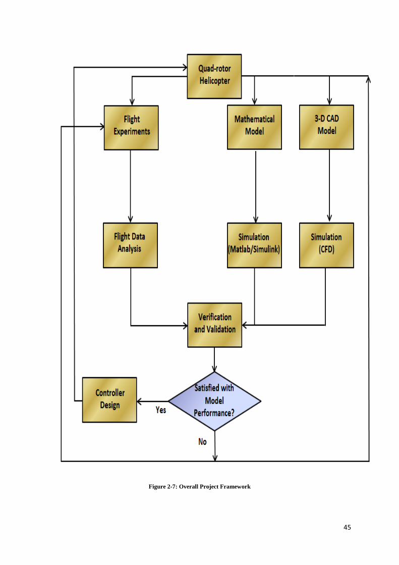
45
Figure 2-7: Overall Project Framework
46
CHAPTER 3
ANALYTICAL DYNAMIC MODEL OF THE QUAD-ROTOR
This chapter presents the development of an analytical dynamic model of the quad-rotor
helicopter using the Newton-Euler Formalism. The force-moment balance is considered,
leading to a set of differential equations of motion, out of which three compute the angular
accelerations of roll, pitch and yaw; and another three compute the linear accelerations in the
x, y and z directions. The actuator (brushless DC motor) dynamics are also considered to
establish its own equation. The set of equations in this case is considered a faithful
mathematical representation of the quad-rotor helicopter.
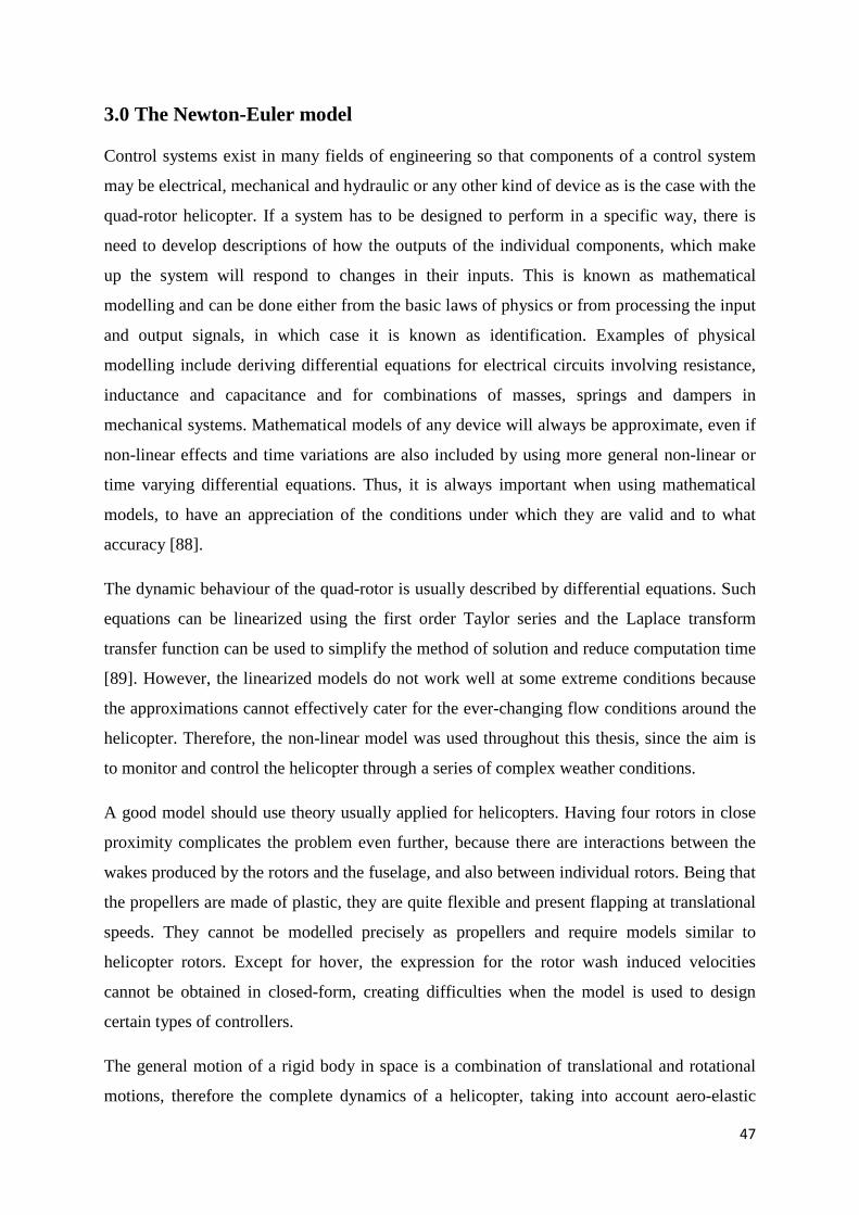
47
3.0 The Newton-Euler model
Control systems exist in many fields of engineering so that components of a control system
may be electrical, mechanical and hydraulic or any other kind of device as is the case with the
quad-rotor helicopter. If a system has to be designed to perform in a specific way, there is
need to develop descriptions of how the outputs of the individual components, which make
up the system will respond to changes in their inputs. This is known as mathematical
modelling and can be done either from the basic laws of physics or from processing the input
and output signals, in which case it is known as identification. Examples of physical
modelling include deriving differential equations for electrical circuits involving resistance,
inductance and capacitance and for combinations of masses, springs and dampers in
mechanical systems. Mathematical models of any device will always be approximate, even if
non-linear effects and time variations are also included by using more general non-linear or
time varying differential equations. Thus, it is always important when using mathematical
models, to have an appreciation of the conditions under which they are valid and to what
accuracy [88].
The dynamic behaviour of the quad-rotor is usually described by differential equations. Such
equations can be linearized using the first order Taylor series and the Laplace transform
transfer function can be used to simplify the method of solution and reduce computation time
[89]. However, the linearized models do not work well at some extreme conditions because
the approximations cannot effectively cater for the ever-changing flow conditions around the
helicopter. Therefore, the non-linear model was used throughout this thesis, since the aim is
to monitor and control the helicopter through a series of complex weather conditions.
A good model should use theory usually applied for helicopters. Having four rotors in close
proximity complicates the problem even further, because there are interactions between the
wakes produced by the rotors and the fuselage, and also between individual rotors. Being that
the propellers are made of plastic, they are quite flexible and present flapping at translational
speeds. They cannot be modelled precisely as propellers and require models similar to
helicopter rotors. Except for hover, the expression for the rotor wash induced velocities
cannot be obtained in closed-form, creating difficulties when the model is used to design
certain types of controllers.
The general motion of a rigid body in space is a combination of translational and rotational
motions, therefore the complete dynamics of a helicopter, taking into account aero-elastic

48
effects, flexibility of the wings, internal dynamics of the actuators and the whole set of
changing variables are quite complex and to a certain degree unmanageable for the purposes
of control. Therefore, it is remarkable to consider a simplified model of a quad-rotor
helicopter formed by a minimum number of states and inputs, but retaining the main features
that must be considered when designing laws that control large sized helicopters.
In this section, the dynamics of a quad-rotor helicopter are modelled using the Newton-Euler
formalism. This can further be divided into the following sub-sections: *Throughout this section, these notations have been adopted: c = cos, s = sin, t = tan.
3.0.1 Coordinate Frames
A coordinate system uses one or more numbers, or coordinates to uniquely determine the
position of a point or other geometric element on a manifold such as Euclidean space. The
order of the coordinates is significant and they are identified by their position in an ordered
tuple. The use of such a system allows problems in geometry to be translated into problems
about numbers and vice versa.
As a starting point, there are two coordinate systems to be clearly defined:
1. The earth inertial frame (E-frame) - The E-frame (OE, XE, YE, ZE) is chosen as the inertial
right-hand reference. XE points toward the North, YE points toward the West, ZE points
upwards respect to the earth and OE is the axis origin. This frame is used to define the
linear position ГE [m] and the angular position θE [rad] of the quad-rotor.
Figure 3-1: The quad-rotor axes definition

49
2. The body-fixed frame of the vehicle (B-frame) - The B-frame (OB, XB, YB, ZB) is
attached to the quad-rotor body. XB points toward the quad-rotor front, YB points toward
the quad-rotor left, ZB points upwards and OB is the axis origin. OB is chosen to coincide
with the centre of mass of the quad-rotor helicopter.
These two coordinates are related through three successive rotations:
Roll: Rotation of φ around the x-axis;
Pitch: Rotation of θ around the y-axis;
Yaw: Rotation of ψ around the z-axis.
The linear velocity ν B [m/s], the angular velocity ωB [rad/s], the forces BF [N] and the
torques Bτ [N m] are defined in this frame. It is relatively easier to formulate differential
equations that describe motion in the body-fixed frame of a vehicle, rather than the earth
inertial frame because the inertia matrix is time-invariant and the advantage of body
symmetry of the quad-rotor helicopter can be taken to simplify the equations. It was also
thought that measurements taken on-board are easily converted to body-fixed frame and the
control forces are almost always given in body-fixed frame [46, 90].
3.0.2 Quad-rotor Modelling Assumptions
A model is a representation of a real physical system and the results of the computation of
any model are only approximations of the actual results that would be observed in real world
conditions, which are mostly very difficult to simulate. Models intentionally simplify reality,
in order to make it tractable. What is important is a good understanding of how the model
simplifies reality. Good modelling assumptions make work easier and don’t adversely affect
the simulations results, but bad assumptions produce results that diverge wildly from reality.
It was very necessary for the following reasonable assumptions to be made concerning the
modelling of the quad-rotor helicopter:
1. The origin of the body-fixed frame OB coincides with the centre of mass (COM) of the
body of the vehicle. Otherwise, another point (COM) should have considered and that
would have significantly complicated the body equations.
2. The axes of the B-frame coincide with the body principal axes of inertia. In this case the
inertia matrix I is diagonal and, once again, the body equations become easier to work
with.

50
3. The acceleration of gravity is constant and perpendicular to the surface of the Earth.
4. The quad-rotor body as well as the propellers will be treated as a rigid body.
5. Being an indoor experiment setup, the helicopter is assumed to fly at low speeds, the air
friction is very low and can be ignored, gyroscopic effects and the aerodynamic torques
can be cancelled.
3.0.3 Quad-rotor Helicopter State Variable definition
The state or set of system variables describe the status of a particular system at any time
instant. Since the primary concern is how system behaviour changes with time, the most
useful state variables are often the rate-of-change variables within any system or
combinations of these variables and their derivatives. For example - in a mechanical system,
the interest is more on the position and/or velocity (rate-of change of position) of a given
component which moves due to an input force. In defining a state variable model, the inputs,
outputs and state variables for the given system are clearly stated. The whole representation is
referred to as a state-space system, which is simply a working region where system
descriptions are represented by states and the rules for the space include rules for operations
on these states.
Figure 3-2: Quad-rotor Configuration Scheme
Let the linear position of the quad-rotor helicopter be a vector ГE. It is normally determined
by the coordinates (x, y, z) of the vector between the origin of the quad-rotor body frame (B-
frame) and the origin of the earth frame (E-frame) with respect to the E-frame as shown in
the equation (3-1) below.

51
=++=Γ
zyx
kzjyixE
(3-1)
Let the attitude (or angular position) of the quad-rotor helicopter be another vector Θ E. This
is defined by the orientation of the B-frame with respect to the E-frame. It is given by three
consecutive rotations (ϕ ,θ ,ψ ) about the main axes. These rotations take the E-frame into the
B-frame.
=Θ
ψθϕ
E (3-2)
Let ξ [+] be the generalised position vector, which is made up of the quad-rotor linear ГE [m]
and angular Θ E [rad] position vectors with respect to the E-frame as shown in the equation
(3-3) below.
=
=
ΘΓ
ψθϕ
ξzyx
E
E
(3-3)
Let ν B and ωB be the quad-rotor linear and angular velocity vectors respectively. The
compositions of the linear and angular velocity vectors are:
=++=
wvu
kwjviuB
ν (3-4)
And
=++=
rqp
krjqipB
ω (3-5)
Similarly, let ν [+] be composed of the quad-rotor linear and angular velocity vectors with
respect to the B-frame as shown in the equation below.

52
=
=
rqpwvu
vω
ν B
B
(3-6)
From equations (3-3) and (3-6), we see that it is possible to combine linear and angular
quantities to give a full representation of a body in space.
3.0.4 Direction Cosine Matrix
The direction cosine matrix is so called because its elements can be determined from the dot
products that involve the direction cosines between corresponding axes of the new and old
coordinate systems. To transform the vectors from the E-frame to the B-frame, a direction
cosine matrix is required. The rotation of one Cartesian coordinate system with respect to
another can always be described by three successive rotations, and the angles of rotation are
called the Euler angles. These angles are specified in diverse ways in different fields of
Science. In this thesis, the rotations are performed by rotating first around x-axis, then around
y axis and finally around the z axis as found in [27, 91]. The matrix is given by:
)(*)(*)(),,( ψθϕψθϕ zyx RRRRR ==Θ (3-7)
The basic (gimbal-like) rotation matrices rotate vectors about the x, y, or z axes, in three
dimensions and are described separately as:
)(ϕxR , rotation around the x-axis.
)(θyR , rotation around the y-axis.
)(ψzR , rotation around the z-axis.
They are represented by:
Figure 3-3: Rotation around the X axis of the angle ϕ (roll)
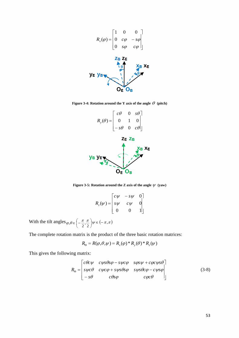
53
−=
ϕϕϕϕϕ
csscRx
00
001)(
Figure 3-4: Rotation around the Y axis of the angle θ (pitch)
−=
θθ
θθθ
cs
scRy
0010
0)(
Figure 3-5: Rotation around the Z axis of the angle ψ (yaw)
−=
10000
)( ψψψψ
ψ cssc
Rz
With the tilt angles
−∈
2,
2, ππθϕ ( )ππψ ,−∈
The complete rotation matrix is the product of the three basic rotation matrices:
)(*)(*)(),,( ψθϕψθϕ zyx RRRRR ==Θ
This gives the following matrix:
−−+
+−=Θ
θϕϕθθϕψϕθψϕθψϕψθψθψϕψϕϕψϕθψψθ
ccscssccssssscccssccsscsssccc
R (3-8)

54
3.0.5 Quad-rotor Kinematics
Kinematics describes the motion of points, objects and system of bodies without considering
the causes of motion. The study of kinematics is usually referred to as the geometry of
motion. To describe motion, kinematics studies the trajectories of points, lines and other
geometric objects and their differential properties such as velocity and acceleration.
Having defined the transformation matrices, we can now find the velocity of the vehicle in
the inertial frame instead of the Body coordinate frame.
The rotation matrix θR is involved in the relationship between the linear velocity ν B [m/s] in
the body-fixed frame and the linear velocity ν E [m/s] in the earth frame as shown below.
−−+
+−=
==
=Γ= ΘΘ•
•
•
•
wvu
ccscssccssssscccssccsscsssccc
wvu
RvR
z
yx
BEE
θϕϕθθϕψϕθψϕθψϕψθψθψϕψϕϕψϕθψψθ
ν (3-9)
++−−+++
++−+=
wccvscuswsccssvsssccucswsccssvcssscucc
E
)()()()()()()()()(
θϕϕθθϕψϕθψϕθψϕψθψθψϕψϕϕψϕθψψθ
ν (3-10)
The relationship between the angular velocity •
ΘE in the earth frame and the angular velocity
in the body-fixed frame is given by
BT ωΘ
•
=ΘE (3-11)
The transfer matrix θT can be found by resolving the Euler angle rates •
ΘE into the body fixed
frame as shown in equation (3-12) below.
=
+
+
=
•
•
•
−
•
−−•
−
•
ψθ
ϕ
ψθϕθϕ
ϕ
θ1111 0
0)()(
0
0)(
00 TRRR
rqp
yxx (3-12)
−=
θϕθϕϕϕθϕθϕ
θ
cccssctcts
T//0
01
(3-13)

55
3.0.6 Quad-rotor Dynamics
Dynamics is concerned with the study of forces and torques together with their effects on
motion, as opposed to kinematics, which studies the motion but does not refer to its causes.
The study of dynamics is based mostly on the fundamental physical laws defined by Isaac
Newton.
The study of dynamics could be linear or rotational. Linear dynamics pertains to objects
moving in a line and involves quantities such as force, mass/inertia, displacement, velocity,
acceleration and momentum. On the other hand, rotational dynamics pertains to objects that
are rotating or moving in a curved path and involves quantities such as torque, moment of
inertia/rotational inertia, angular displacement, angular velocity, angular acceleration and
angular momentum.
Since it is known from Euler’s first axiom of Newton’s second law of motion, that the
applied force in the E-frame is the product of the vehicle’s mass and its acceleration, i.e.
maonacceleratimassForce =×=
It can be deduced that
)()( 2
2
dtdm
dtdvmF
EE Γ
== (3-14)
From equation (3-9), 2
2
dtd EΓ is given by
=Γ=Γ
••
••
••
••
z
yx
dtd E
E
2
2
(3-15)
This leads to ••
Γ= EE mF (3-16)
And
=
==Γ=Γ=
=
••
••
••
•
•
•
•••
z
yx
m
z
yx
dtdmv
dtdm
dtdmm
FFF
F EEE
z
y
xE (3-17)
Where EF has components in x, y and z. Multiplying both sides by the direction cosine
matrix in equation (3-8) gives the following
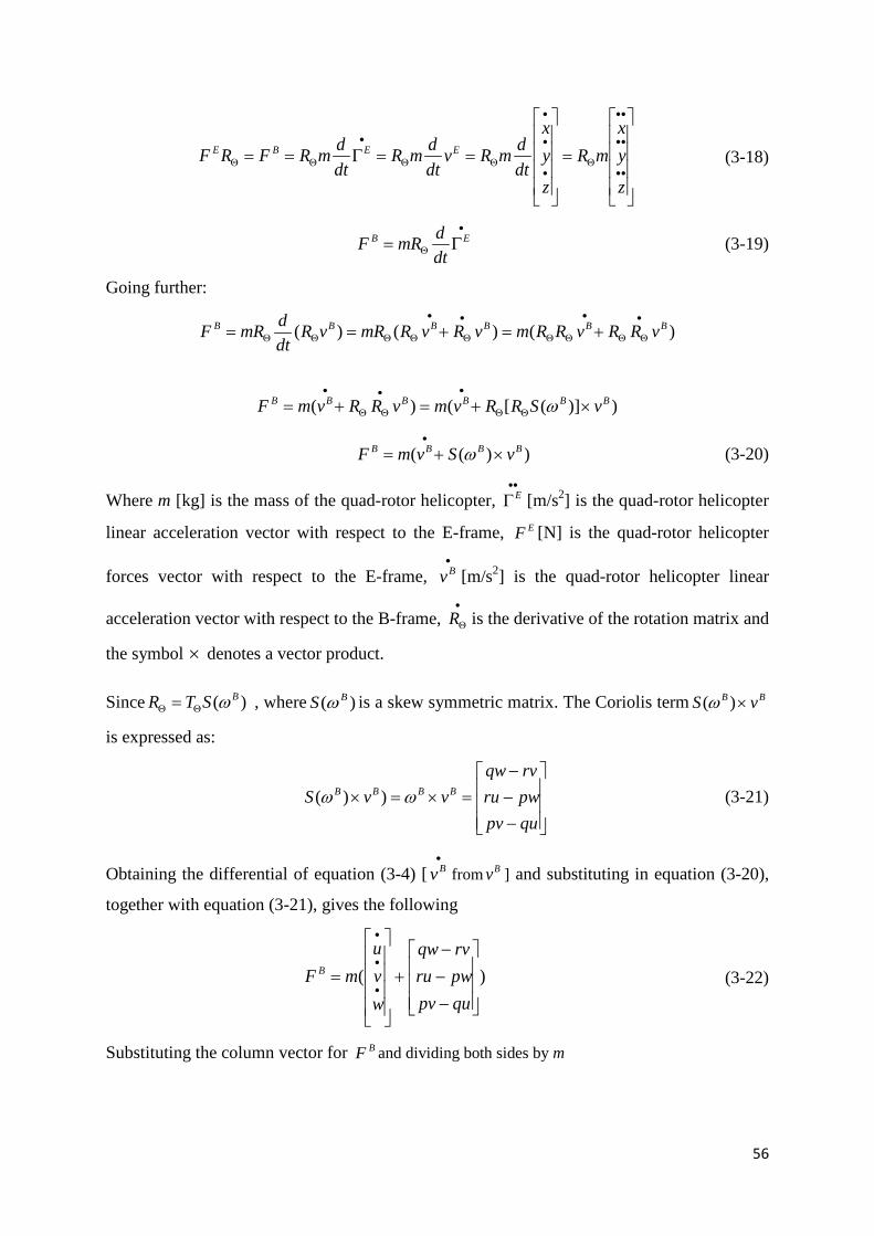
56
=
==Γ==••
••
••
Θ•
•
•
ΘΘ
•
ΘΘ
z
yx
mR
z
yx
dtdmRv
dtdmR
dtdmRFRF EEBE (3-18)
•
Θ Γ= EB
dtdmRF (3-19)
Going further:
)()()( BBBBBB vRRvRRmvRvRmRvRdtdmRF
•
ΘΘ
•
ΘΘ
•
Θ
•
ΘΘΘΘ +=+==
))]([()( BBBBBB vSRRvmvRRvmF ×+=+= ΘΘ
••
ΘΘ
•
ω
))(( BBBB vSvmF ×+=•
ω (3-20)
Where m [kg] is the mass of the quad-rotor helicopter, ••
ΓE [m/s2] is the quad-rotor helicopter
linear acceleration vector with respect to the E-frame, EF [N] is the quad-rotor helicopter
forces vector with respect to the E-frame, •Bv [m/s2] is the quad-rotor helicopter linear
acceleration vector with respect to the B-frame, •
ΘR is the derivative of the rotation matrix and
the symbol × denotes a vector product.
Since )( BSTR ωΘΘ = , where )( BS ω is a skew symmetric matrix. The Coriolis term BB vS ×)(ω
is expressed as:
−−−
=×=×qupvpwrurvqw
vvS BBBB ωω ))( (3-21)
Obtaining the differential of equation (3-4) [•Bv from Bv ] and substituting in equation (3-20),
together with equation (3-21), gives the following
)(
−−−
+
=•
•
•
qupvpwrurvqw
wvu
mF B (3-22)
Substituting the column vector for BF and dividing both sides by m
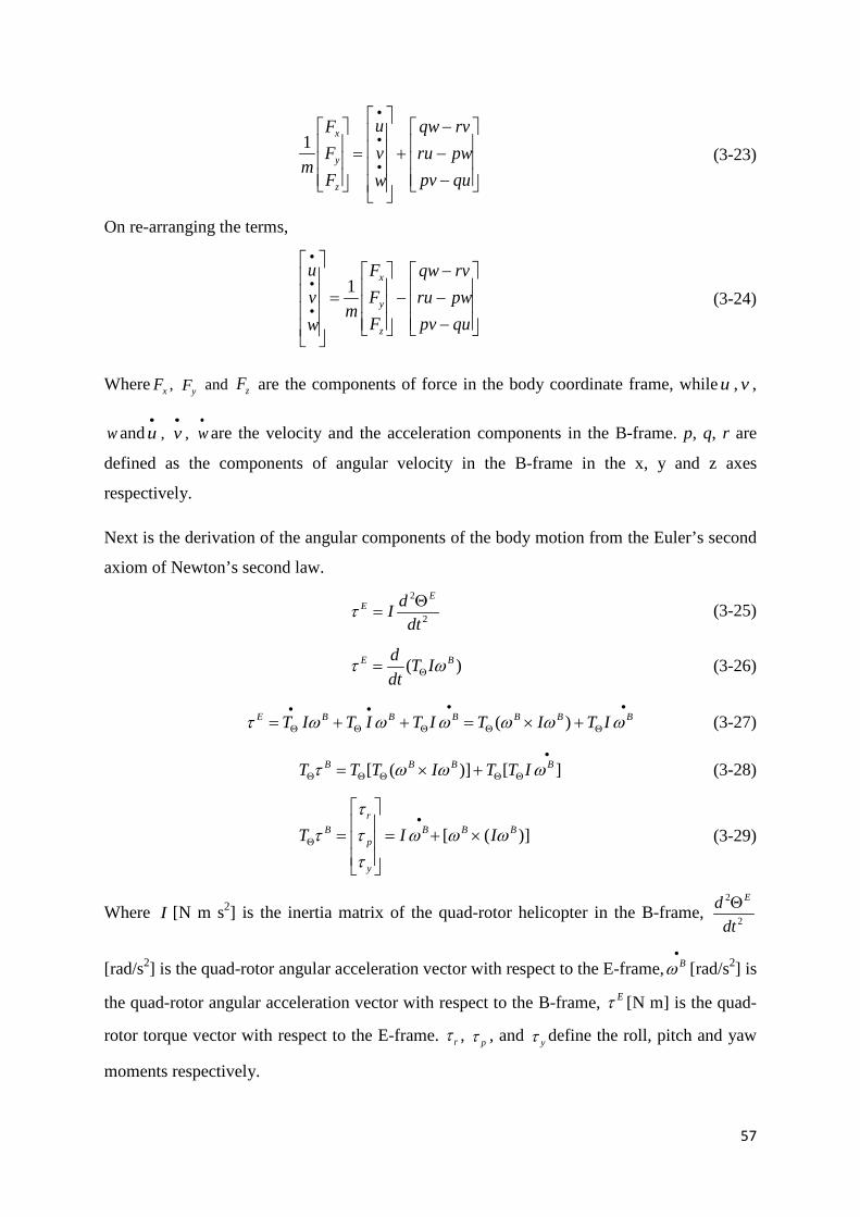
57
−−−
+
=
•
•
•
qupvpwrurvqw
wvu
FFF
mz
y
x1 (3-23)
On re-arranging the terms,
−−−
−
=
•
•
•
qupvpwrurvqw
FFF
mwvu
z
y
x1 (3-24)
Where xF , yF and zF are the components of force in the body coordinate frame, while u , v ,
w and•
u , •
v , •
w are the velocity and the acceleration components in the B-frame. p, q, r are
defined as the components of angular velocity in the B-frame in the x, y and z axes
respectively.
Next is the derivation of the angular components of the body motion from the Euler’s second
axiom of Newton’s second law.
2
2
dtdI
EE Θ
=τ (3-25)
)( BE ITdtd ωτ Θ= (3-26)
•
ΘΘ
•
Θ
•
Θ
•
Θ +×=++= BBBBBBE ITITITITIT ωωωωωωτ )( (3-27)
•
ΘΘΘΘΘ +×= ][)]([ BBBB ITTITTT ωωωτ (3-28)
)]([ BBB
y
p
rB IIT ωωω
τττ
τ ×+=
=•
Θ (3-29)
Where I [N m s2] is the inertia matrix of the quad-rotor helicopter in the B-frame, 2
2
dtd EΘ
[rad/s2] is the quad-rotor angular acceleration vector with respect to the E-frame,•Bω [rad/s2] is
the quad-rotor angular acceleration vector with respect to the B-frame, Eτ [N m] is the quad-
rotor torque vector with respect to the E-frame. rτ , pτ , and yτ define the roll, pitch and yaw
moments respectively.

58
=
=
zz
yy
xx
zzzyzx
yzyyyx
xzxyxx
II
I
IIIIIIIII
I00
0000
(3-30)
( 0====== zyzxyzyxxzxy IIIIII , since the quad-rotor helicopter is assumed to be
symmetric in nature)
From equation (3-29), the angular acceleration is given by the equation
)]]([[1 BBBB ITI ωωτω ×−= Θ−
•
(3-31)
Also from equation (3-30), we can find the inverse of the inertia matrix, which is given as
=−
zz
yy
xx
I
I
I
I
100
010
001
1 (3-32)
From equation (3-5), differentiating the angular velocity gives
=•
•
•
•
r
q
pBω (3-33)
Substituting and simplifying in equation (3-31),
]]00
0000
[[[1
×
−=
= Θ−
•
•
•
•
rqp
II
I
rqp
TI
r
q
p
zz
yy
xxBB τω
][[][[ 11
×
−=
+−−−+−
−−×
−=
= Θ−
Θ−
•
•
•
•
zz
yy
xxB
zzzyzx
yzyyyx
xzxyxxBB
rIqIpI
rqp
TIrIqIpIrIqIpI
rIqIpI
rqp
TI
r
q
p
ττω
][][[ 11
−−−
−=
×
−=
= Θ−
Θ−
•
•
•
•
xxyy
zzxx
yyzzB
zz
yy
xxBB
qpIpqIprIrpIrqIqrI
TIrIqIpI
rqp
TI
r
q
p
ττω

59
][1
−−−
−
=
= −
•
•
•
•
xxyy
zzxx
yyzz
y
p
rB
qpIpqIprIrpIrqIqrI
I
r
q
p
τττ
ω
From equation (3-32), substitution can be made for 1−I
][
100
010
001
−−−
−
=
=•
•
•
•
xxyy
zzxx
yyzz
y
p
r
zz
yy
xx
B
qpIpqIprIrpIrqIqrI
I
I
I
r
q
p
τττ
ω
Simplifying further,
−
−
−
−
=
•
•
•
zzxxyy
yyzzxx
xxyyzz
zz
y
yy
p
xx
r
IpqII
IprII
IqrII
I
I
I
r
q
p
)(
)(
)(
τ
τ
τ
(3-34)
3.0.7 Quad-rotor Aerodynamic Forces
There would normally be four forces acting on any helicopter in flight. These forces are lift,
thrust, weight and drag. A very good distribution of these forces while the helicopter is aloft
ensures movement in the intended direction.
3.0.7.1 Lift and Thrust forces
A fluid flowing past the surface of a body exerts a force on it. Lift is the component of this
force that is perpendicular to the relative fluid flow. This force is generated by the spinning
rotor to keep the helicopter in the air.
Thrust is also generated by the rotation of the rotor blades. This is the force that propels the
helicopter through the air. For the quad-rotor helicopter, thrust can be forward, backward,
sideward and vertical.
The quad-rotor helicopter’s motion (vertical and horizontal) is affected by actions of the four
propellers. The resultant of lift and thrust determines the direction of movement of the
helicopter.
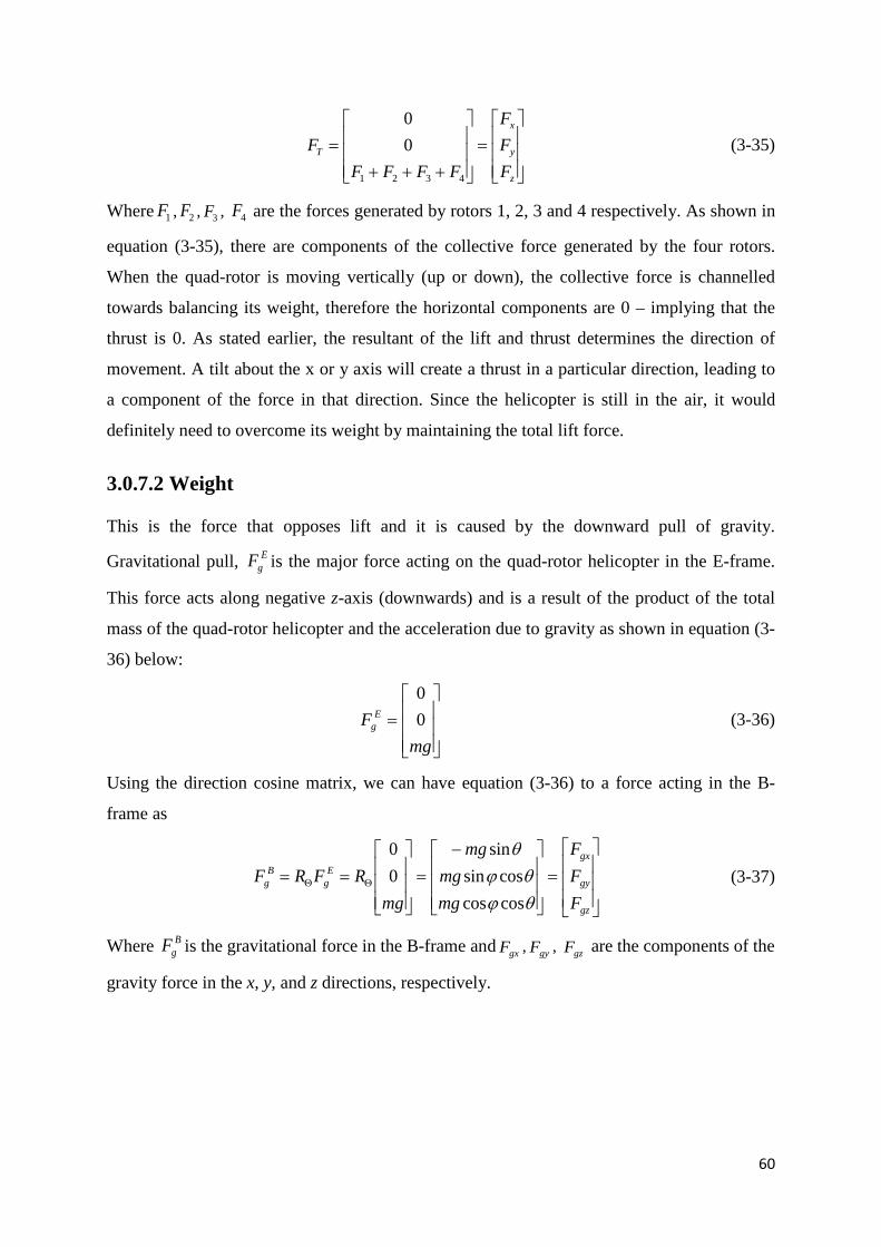
60
=
+++=
z
y
x
T
FFF
FFFFF
4321
00
(3-35)
Where 1F , 2F , 3F , 4F are the forces generated by rotors 1, 2, 3 and 4 respectively. As shown in
equation (3-35), there are components of the collective force generated by the four rotors.
When the quad-rotor is moving vertically (up or down), the collective force is channelled
towards balancing its weight, therefore the horizontal components are 0 – implying that the
thrust is 0. As stated earlier, the resultant of the lift and thrust determines the direction of
movement. A tilt about the x or y axis will create a thrust in a particular direction, leading to
a component of the force in that direction. Since the helicopter is still in the air, it would
definitely need to overcome its weight by maintaining the total lift force.
3.0.7.2 Weight
This is the force that opposes lift and it is caused by the downward pull of gravity.
Gravitational pull, EgF is the major force acting on the quad-rotor helicopter in the E-frame.
This force acts along negative z-axis (downwards) and is a result of the product of the total
mass of the quad-rotor helicopter and the acceleration due to gravity as shown in equation (3-
36) below:
=
mgF E
g 00
(3-36)
Using the direction cosine matrix, we can have equation (3-36) to a force acting in the B-
frame as
=
−=
== ΘΘ
gz
gy
gxE
gB
g
FFF
mgmg
mg
mgRFRF
θϕθϕ
θ
coscoscossin
sin00
(3-37)
Where BgF is the gravitational force in the B-frame and gxF , gyF , gzF are the components of the
gravity force in the x, y, and z directions, respectively.

61
3.0.7.3 Drag Force
Drag is the force that opposes the motion of an aircraft through the air. It is primarily a
function of airspeed, directly opposing lift and thrust. It is normally computed as a product of
the coefficient of drag and the square of the velocity in each of the three axes.
=
2
2
2
)(21
)(21
)(21
EzcDz
EycDy
ExcDx
ED
VAC
VAC
VAC
F
ρ
ρ
ρ
(3-38)
Where A is the cross-sectional area, ρ the air density; xV , yV , zV are the E-frame
components of velocity. DxC , DyC , DzC are the drag coefficients in each of the three axes. The
transformation matrix can also be used in this case to get the B-frame components of the drag
force.
=
==•
•
•
Θ
Dz
Dy
Dx
cDz
cDy
cDx
ED
BD
FFF
zAC
yAC
xAC
FRF
2
2
2
212121
ρ
ρ
ρ
(3-39)
The quad-rotor helicopter operates at airspeeds low enough for us to assume that the drag
force is very little and therefore can be ignored as confirmed in [90].
3.0.7.4 Collective Force acting on the Quad-rotor
The total force is the sum of the lift/thrust, weight and drag forces:
+
+
=
=
Tz
Ty
Tx
Dz
Dy
Dx
gz
gy
gx
z
y
x
B
FFF
FFF
FFF
FFF
F (3-40)
++++
+
−=
=
•
•
•
43212
2
2
00
212121
coscoscossin
sin
FFFFzAC
yAC
xAC
mgmg
mg
FFF
F
cDz
cDy
cDx
z
y
x
B
ρ
ρ
ρ
θϕθϕ
θ

62
+++++
+
+−
=
•
•
•
)(21coscos
21cossin
21sin
43212
2
2
FFFFzACmg
yACmg
xACmg
FFF
cDz
cDy
cDx
z
y
x
ρθϕ
ρθϕ
ρθ
(3-41)
3.0.8 Quad-rotor Moments (Torques)
The moment or torque of a force about a turning point is the product of the force and the
perpendicular distance to the force from the turning point. For an object to be in equilibrium,
the sum of clockwise and anticlockwise moments about a turning point must be equal to 0.
This is the exact principle the quad-rotor helicopter uses to remain stable as it flies around
with its two pairs of counter-rotating blades.
If iτ is the torque generated by each motor, the rolling moment rτ is produced by changing
the speeds of the right and left motors.
)( 424242 FFllFlFr −=−=−= τττ (3-42)
Similarly the pitching moment pτ (torque) is produced by changing the speeds of the front
and rear motors.
)( 313131 FFllFlFp −=−=−= τττ (3-43)
Considering Newton’s third law of motion, which states that for every action there is an equal
and opposite reaction; the drag of the propellers produces a yawing moment on the quad-rotor
helicopter. Consequently, the total yawing moment is obtained from all the rotor speeds and
is given by
dFFFFmmmmmy )( 43214321 −+−=−+−== ∑ ττττττ (3-44)
3.0.9 Quad-rotor Moments of Inertia
A moment of inertia is the mass property of a rigid body that defines the torque needed for a
desired change in angular velocity about an axis of rotation. This moment depends on the
shape of the body, amount and distribution of its mass and may differ around one axis of
rotation and another.

63
3.0.9.1 Moment of Inertia about the x-axis
In deriving the moment of inertia around the x-axis, the central hub and all the motors of the
quad-rotor helicopter are assumed to be cylindrical in shape.
Figure 3-6: Quad-rotor moments of inertia
Let the following parameters be used as masses of motors and central hub 1m , 3m , cm ; radii 1r
, 3r , cr and height 1h , 3h , ch , respectively. Here, only the rolling motion is considered.
Firstly, the moment of inertia about the x-axis would be due to the motion of the main body
and the front and rear motors about x-axis. Secondly, the moment of inertia would be due to
the motion of the left and right motors about the x-axis.
cxx IIIII +++= 314,2 (3-45)
The moment of inertia of a cylinder about an axis perpendicular to its body, as specified in
[94], thus the moment of inertia due to main body and the two motors are given by:
124
22
,cccc
xchmrmI += (3-46)
124
211
211
,1hmrmI x += (3-47)
124
233
233
,3hmrmI x += (3-48)
The moment of inertia of two identical spheres connected together by a horizontal arm,
rotating about a vertical axis, which is passing through the centre of the arm and is
perpendicular to it, according to [92, 93] can be approximated to be 2
,42 2 lmI rx =− (3-49)
Since the motors are assumed to be identical:
rmmmmm ==== 4321 , rrrrrr ==== 4321 and rhhhhh ==== 4321

64
Finally, the total inertia about the x-axis is found by substituting equations (3-46), (3-47), (3-
48) and (3-49) in equation (3-45)
2233
233
211
211
22
2124124124
lmhmrmhmrmhmrmI rcccc
xx ++++++=
22222
262124
lmhmrmhmrmI rrrrrcccc
xx ++++= (3-50)
3.0.9.2 Moment of Inertia about the y-axis
In the same way, the moment of inertia about the y-axis can be found because of the earlier
assumption that the quad-rotor helicopter structure is symmetrical and the motors are
identical. Going through the process that was done in finding the moment of inertia about the
x-axis gives
22222
262124
lmhmrmhmrmI rrrrrcccc
yy ++++= (3-51)
3.0.9.3 Moment of Inertia about the z-axis
The moment of inertia about the z-axis will be due to the motion of the main body and also
due to the motion of all the motors [92, 93]. The moment of inertia due to the main body can
be found to be:
2
2
,cc
zcrmI = (3-52)
The moment of inertia due to all the motors can be approximated to be: 2
,4321 4 lmI rz =−−− (3-53)
Therefore, the total inertia about z-axis is the sum of the two:
22
42
lmrmI rcc
zz += (3-54)
3.0.10 Equations of Motion
Putting together the equations (3-24) and (3-41) gives:
−−−
−
+++++
+
+−
=
•
•
•
•
•
•
qupvpwrurvqw
FFFFzACmg
yACmg
xACmg
mwvu
cDz
cDy
cDx
)(21coscos
21cossin
21sin
1
43212
2
2
ρθϕ
ρθϕ
ρθ

65
−++++++
−++
−++−
=
•
•
•
•
•
•
)()(121coscos
)(21cossin
)(21sin
43212
2
2
pvquFFFFm
zACm
g
rupwyACm
g
qwrvxACm
g
wvu
cDz
cDy
cDx
ρθϕ
ρθϕ
ρθ
(3-55)
−+++++
−+−+−
=
•
•
•
)()(1coscos
)(cossin)(sin
4321 pvquFFFFm
g
rupwgqwrvg
wvu
θϕ
θϕθ
(3-56)
In the same way combining equations (3-18) and (3-41), gives:
=Γ=
=
••
••
••
Θ
•
Θ
z
yx
mRdtdmR
FFF
F E
z
y
xB
The terms can be re-arranged to give
=
−
Θ••
••
••
z
y
x
FFF
Rm
z
yx
11
Since it is known from equation (3-41) that
++++
+
−=
•
•
•
43212
2
2
00
212121
coscoscossin
sin
FFFFzAC
yAC
xAC
mgmg
mg
FFF
cDz
cDy
cDx
z
y
x
ρ
ρ
ρ
θϕθϕ
θ
Substitutions can be made and the equation simplified further, remembering that the matrix
representing the drag forces can be reduced to 0 as stated earlier.
]00
coscoscossin
sin[1
4321
1
++++
−=
−
Θ••
••
••
FFFFmgmg
mgR
mz
yx
θϕθϕ
θ
On simplifying, it ends up as follows

66
+++
−+++
++++
=
••
••
••
)cos)(cos(1
)sincoscossin)(sin(1
)sincoscossin)(sin(1
4321
4321
4321
θϕ
ϕψϕθψ
θψϕψϕ
FFFFm
FFFFm
FFFFm
z
yx
(3-57)
The next section describes the actuator model, where relationships between voltage, angular
velocity of propeller and thrust were found, leading to a modification of equation (3-57) and a
derivation of the angular acceleration equations to form the quad-rotor analytical dynamic
model. The final equations of motion are listed at the end of section 3.2.
3.1 Actuator Dynamics (DC-motor)
The DC-motor is an actuator which converts electrical energy into mechanical energy (and
vice versa). It is composed of two interactive electromagnetic circuits. The first one (called
rotor) is free to rotate around the second one (called stator) which is fixed instead. In the
rotor, several groups of copper windings are connected in series and are externally accessible
thanks to a device called commutator. In the stator, two or more permanent magnets impose a
magnetic field which affects the rotor. By applying a DC-current flow into the windings, the
rotor turns because of the force generated by the electrical and magnetic interaction. Thanks
to the rotor and the commutator geometries, the motor keeps turning while supplied by a DC-
voltage on its terminals.
The DC-motor has a well-known model which binds electrical and mechanical quantities.
This model is composed of the series of a resistor R [Ω], an inductor L [H] and a voltage
generator e [V]. The resistor represents the Joule loss due to the current flow into the copper
conductor. Its value depends on geometric and material characteristics such as wire
resistivity, length and section. The inductor behaviour derives from the shape of the motor
wires which are winded in the middle of the rotor. Lastly, the generator e (called also BEMF)
supplies a voltage proportional to the motor speed. The model is represented in the figure 3-7
below.
Figure 3-7: Schematic of a DC Motor

67
The circuit of the DC-motor is controlled by a real voltage generator v [V], which gives the
control input. In theory, another resistor should be added in series of the voltage generator
representing the driver losses. However, in a good project, the generator losses are kept low
therefore it is possible to neglect them in the model. The basic electrical circuit is shown
figure 3-8 below.
Figure 3-8: DC Motor circuit
By applying Kirchhoff’s voltage law, it follows that.
evvv LR ++= (3-58)
Where v R [V] is the voltage across the resistor R and v L [V] is the voltage across the
inductor L. The equation above can be rewritten as in the next equation.
Ω+∂∂
+= ektiLRiv (3-59)
Where i [A] is the motor current, eK [Vs/rad] is called the motor constant and Ω [rad/s] is
the motor angular speed. The first addend has been changed using the Ohm’s law v R= Ri ,
while the second one using the inductor differential equation v L=tiL
∂∂ . The last member of
the equation shows that mechanics and electrics are correlated.
The contribution of the inductor part is important to determine the characteristic of the DC-
motor driver. However it is often neglected in the mechanics computation because of the
reasons that follow:
a) A greater percentage of the motors used in robotics show very small inductance because
of design optimization.
b) The response time of the electrical part is always much faster than the mechanical part,
hence the speed of the overall system will be determined by the slowest contribution.
c) It is much easier to solve a first order differential equation rather than a second order one.
For the reasons mentioned above, the inductor effect was neglected in this thesis. Therefore
the equation above can be simplified according to the one below.

68
Ω+= ekRiv
The dynamics of the motor is described by the following equation.
dmJ ττ −=Ω•
(3-60)
Where J [Nms2] is the total motor moment of inertia, •
Ω [rad/s2] is the motor angular
acceleration, mτ [Nm] is the motor torque and dτ [Nm] is the load torque. When the motor
torque mτ and the load torque dτ are not the same, then there is an acceleration (or
deceleration) of the motor angular speed Ω . This variation of speed depends also on the total
motor moment of inertia J : the smaller the value of J , the higher the acceleration. Figure 3-
9 below is a sketch of the simplified mechanic structure.
Figure 3-9: Simplified DC motor system
The motor torque mτ is proportional to the electrical current i through qk [Nm/A]: mτ = qk i .
Hence it can be written as
dqiJ τ−=Ω k .
A differential equation in Ω can be easily derived:
vRR
J qd
qe kkk +−Ω−=Ω
•
τ (3-61)
It must be pointed out that the two constants ek and qk have the almost the same value even
though the units of measurement differ. This mismatch comes from the electric EP [W] and
mechanic MP [Nm/s] power balance [4].
EP = MP qeqmM
eE kkikP
ikeiP≈⇒
Ω=Ω=Ω==
τ (3-62)
3.1.1 Voltage and Angular Velocity of Propeller
Since the voltage inputs (V) to motors affect the rotational speed (Ω) of propellers.
iReV =−
69
From equation (3-60), the dynamics of the motor is described by the following equation
•
Ω=− Jdm ττ
The above equation states that when the motor torque mτ and the drag torque dτ are not equal
there is an acceleration (or deceleration). This variation of speed depends also on the rotor
inertia J . The smaller the value of J , the higher the acceleration. The back electromotive-
force voltage being proportional to the motor speed gives
Ω= eKe
Also, the motor torque is known to be proportional to field current
ikqm =τ
On substituting, it gives rise to
Ω+Ω
+=
•
eqq
d kk
RJkRV τ (3-63)
The drag torque is also known to be proportional to the square of propeller’s speed, leading to
2Ω= Ddτ (3-64)
The relationship between angular velocity and voltage can then be obtained as
Ω+Ω
+Ω
=
•
eqq
kk
RJk
RDV2
(3-65)
3.1.2 Voltage and Thrust
The voltage is the input of the quad-rotor plant. Thrust force (FT) is produced by each rotor
through the torque applied by brushless DC motor. As stated earlier, the motor torque is
proportional to field current
ikqm =τ
Making i the subject of the formula, gives
ikq
m =τ (3-66)
70
The electrical power is calculated by using Joule’s law.
Vk
IVPq
mτ== (3-67)
The mechanical power output of the motor’s efficiency is given by
Vk
PPq
mm
τηη == (3-68)
The Figure of merit f of the propeller is defined as the ratio of the induced power hP to the
power put into the propeller mP .
m
h
PPf = (3-69)
Re-arranging and substituting for mP from equation (3-68), gives
Vk
fPq
mh
τη= (3-70)
The ideal power is the thrust force times the speed it is applied at. At hover hP is
hh FvP =
hq
m FvVk
f =τη (3-71)
Using the momentum theory,
AFvh ρ2
=
Substituting for hv in equation (3-70), gives
AFFV
kf
q
m
ρτη
2= (3-72)
The torque is proportional to the thrust with constant ratio tk depending on the geometry of the
blade.

71
Fktm =τ
Substituting for mτ in equation (3-72), gives
AFFV
kFkfq
t
ρη
2=
The relationship between thrust and voltage input is then established as:
2
2
2 Vk
kfAFq
t
=
ηρ (3-73)
3.1.3 Rolling Moment
As shown in equation (3-42), the rolling moment caused by the roll actuators action can be
defined as:
)( 42 FFlr −=τ
And••
= ϕτ xxr I , therefore
)( 42 FFlI xx −=••
ϕ (3-74)
From equation (3-73), the thrust force is defined as 2
2
2 Vk
kfAFq
t
=
ηρ
Substituting in equation (3-74), gives
)2()2( 24
2
22
2
Vk
kfAVk
kfAlIq
t
q
txx
−
=
•• ηρηρϕ
Simplifying further, leads to the final equation for roll angular acceleration, which is as
follows
)(2 24
22
2
VVk
kfI
Alq
t
xx
−
=
•• ηρϕ (3-75)

72
3.1.4 Pitching Moment
From equation (3-43), the pitching moment caused by the pitch actuators action can be
defined as:
)( 13 FFlp −=τ
And••
= θτ yyp I , therefore
)( 42 FFlI yy −=••
θ (3-76)
Substituting for the thrust force from equation (3-73), gives
)2()2( 21
2
23
2
Vk
kfAVk
kfAlIq
t
q
tyy
−
=
•• ηρηρθ
Simplifying further, leads to the final equation for pitch angular acceleration, which is as
follows
)(2 21
23
2
VVk
kfI
Alq
t
yy
−
=
•• ηρθ (3-77)
3.1.5 Yawing Moment
The yaw moment is caused by a counter-torque imbalance. From equation (3-44), the torque
about the z-axis is generally defined as:
dFFFFmmmmmy )( 43214321 −+−=−+−== ∑ ττττττ
Each motor supplies machine torque mτ which is balanced by the drag torque so the net
torque on propeller is:
•
Ω=− Jdm ττ
Making mτ the subject, gives
dm J ττ +Ω=•
(3-78)

73
The yaw torque along the z-axis is given by:
4231 mmmmzzy I ττττψτ −−+==••
(3-79)
Substituting equation (3-78) in equation (3-79), gives
44223311 ddddzz JJJJI ττττψ −Ω−−Ω−+Ω++Ω=••••••
(3-80)
Re-arranging the equation (3-80), leads to
)()( 42314231 ddddzz JI ττττψ −−++Ω−Ω−Ω+Ω=••••••
(3-81)
Since it is assumed in equation (3-64) that the drag torque is proportional to the square of
propeller’s speed - 2Ω= Ddτ ; substituting in equation (3-81) leads to
)()( 24
22
23
214231 Ω−Ω−Ω+Ω+Ω−Ω−Ω+Ω=
••••••
DJIzzψ
Simplifying further, gives the final equation for yaw angular acceleration as follows
)()( 24
22
23
214231 Ω−Ω−Ω+Ω+Ω−Ω−Ω+Ω=
••••••
zzzz ID
IJψ (3-82)
3.1.6 Acceleration along the x-axis
From equation (3-57), the acceleration along the x-axis, caused by actuators action is defined
as:
)sinsincossin)(cos(14321 ψϕψθϕ ++++=
••
FFFFm
x (3-83)
Substituting equation (3-73), which defines the thrust force and simplifying further, gives the
final equation for linear acceleration in the x-direction as follows
( ) )sinsincossin(cos2 24
23
22
21
2
ψϕψθϕηρ++++
=
••
VVVVk
kfm
Axq
t (3-84)
3.1.7 Acceleration along the y-axis
Similar to that of the x-axis, it was shown in equation (3-57) that actuators action produces
the following acceleration, which acts along the y-axis:

74
( )ϕψϕθψ sincoscossinsin)(14321 −+++=
••
FFFFm
y (3-85)
Substituting equation (3-73), which defines the thrust force and simplifying further, gives the
final equation for linear acceleration in the y-direction as follows
( )( )ϕψϕθψηρ sincoscossinsin2 24
23
22
21
2
−+++
=
••
VVVVk
kfm
Ayq
t (3-86)
3.1.8 Acceleration along z-axis
A lift force perpendicular to the plane of the propellers is generated by the spin of the four
propellers. This implies that when the roll and pitch angles are zero, the force in totality acts
along the z-axis. On the contrary, when one of the two angles is non-zero, only a component
of the total forces ϕθ coscosF acts along z-axis, while the other component(s) act in the x or
y directions to propel the quad-rotor helicopter in a particular direction. The weight of the
helicopter always acts along the negative z-axis; therefore this component of force has to
cancel it out in order to lift the vehicle into the air. As shown in equation (3-57), the
acceleration along the z-axis as a result of the action of the actuators is given as
ϕθ coscos)(14321 FFFF
mz +++=••
(3-87)
But the weight has to be taken into account,
mg−
The net force at the centre of mass of the vehicle is then given by
mgFFFFzmF −+++==••
ϕθ coscos)( 4321 (3-88)
Where m is the net mass of the quad-rotor helicopter. Since equation (3-73) has it that
2
2
2 VK
KfAFq
t
=
ηρ
Substituting in equation (3-88) and simplifying further, gives the final equation for linear
acceleration in the z-direction as follows
( )( ) gVVVVk
kfm
Azq
t −+++
=
••
ϕθηρ coscos2 24
23
22
21
2
(3-89)

75
3.2 Chapter Summary
Design and analysis of any control system is usually started by carefully considering a
mathematical model of the physical system. The model is very important because it gives a
description of how the system responds to the inputs given to it. An adequate dynamic system
modelling of the quad-rotor helicopter involves a faithful mathematical representation of the
whole system, usually described by differential equations.
Equations (3-65), (3-75), (3-77), (3-82), (3-84), (3-86) and (3-89) make up the analytical
dynamic model of the quad-rotor helicopter that has been used throughout this thesis. These
are summarized in equation (3-90) below.
( )
( )( )
( )( )
−+++
−+++
++++
Ω−Ω−Ω+Ω+Ω−Ω−Ω+Ω
−
−
Ω+Ω
+Ω
=
••••
•
••
••
••
••
••
••
gVVVVk
kfm
A
VVVVk
kfm
A
VVVVk
kfm
A
ID
IJ
VVk
kfI
Al
VVk
kfI
Al
kk
RJk
RD
z
yx
V
q
t
q
t
q
t
zzzz
q
t
yy
q
t
xx
eqq
ϕθηρ
ϕψϕθψηρ
ψϕψθϕηρ
ηρ
ηρ
ψθ
ϕ
coscos2
sincoscossinsin2
)sinsincossin(cos2
)()(
)(2
)(2
24
23
22
21
2
24
23
22
21
2
24
23
22
21
2
24
22
23
214231
21
23
2
24
22
2
2
(3-90)
76
CHAPTER 4
SIMULATION OF THE QUAD-ROTOR ANALYTICAL DYNAMIC
MODEL IN MATLAB/SIMULINK
This chapter shows an implementation of the quad-rotor non-linear analytical dynamic model
using block libraries in Matlab/Simulink R2013a software. Calibration of the model and
preliminary calculations are then carried out to ensure that the model performs as expected
and to determine the operating point parameters. Simulations are run to investigate the open
loop flight dynamics.

77
4.0 Matlab/Simulink Software
Simulating the analytical dynamic model of the quad-rotor helicopter is necessary when
designing a controller as it reduces potential risks, design errors, cost and saves time. The
systems have to be simulated and tested rigorously to get a high degree of precision. This also
ensures a good understanding of the helicopter’s responses to its rotor speed changes and
enables realistic constraints to be included in the development of a suitable controller.
Matlab is a high-level technical computing language and interactive environment for
algorithm development, data visualization, data analysis and numeric computation [94]. As
real-world systems have to respond to both continuous and instantaneous changes, Matlab is
an invaluable tool because of its features that support such and it is widely used in
engineering and science. It is very easy to understand and has many features of a
programming language or a simple calculator. Matlab’s code optimization enhances quick
performance of matrix operations and errors are easily detected and fixed since it is an
interpreted language. Its foremost flaw is that it sometimes turns out to be slow.
Simulink is an extension of Matlab, which provides an atmosphere for multi-domain
simulation and model-based design for dynamic and embedded systems. It provides an
interactive graphical environment and a customizable set of block libraries which allow for
design, simulation, implementation, and testing of a variety of time-varying systems. Prior to
the development of simulation systems, scientists and engineers had to write computer codes
(programs) to represent the mathematical models of dynamic systems in a suitable
programming language. In Simulink, the computer codes are the block diagrams and the use
of these blocks removes the risks of a user’s error in writing the computer codes or the risk
that the computer program may not precisely implement the block diagram. The potential
productivity improvement and cost savings realized from the block diagram approach to
programming is dramatic.
Matlab and Simulink are products of the MathWorks. These two outstanding software
packages for scientific and engineering computations are used in many research and
educational establishments, in the aerospace, telecommunications and automotive industries;
for environmental applications and many more. Matlab and Simulink enable researchers to
solve many advanced numerical problems rapidly and efficiently [94]. The Matlab and
Simulink environments are incorporated into one entity, and thus it is easy to analyse,
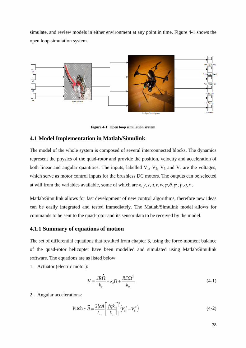
78
simulate, and review models in either environment at any point in time. Figure 4-1 shows the
open loop simulation system.
Figure 4-1: Open loop simulation system
4.1 Model Implementation in Matlab/Simulink
The model of the whole system is composed of several interconnected blocks. The dynamics
represent the physics of the quad-rotor and provide the position, velocity and acceleration of
both linear and angular quantities. The inputs, labelled V1, V2, V3 and V4 are the voltages,
which serve as motor control inputs for the brushless DC motors. The outputs can be selected
at will from the variables available, some of which are rqpwvuzyx ,,,,,,,,,,, ψθϕ .
Matlab/Simulink allows for fast development of new control algorithms, therefore new ideas
can be easily integrated and tested immediately. The Matlab/Simulink model allows for
commands to be sent to the quad-rotor and its sensor data to be received by the model.
4.1.1 Summary of equations of motion
The set of differential equations that resulted from chapter 3, using the force-moment balance
of the quad-rotor helicopter have been modelled and simulated using Matlab/Simulink
software. The equations are as listed below:
1. Actuator (electric motor):
qe
q kRDk
kJRV
2Ω+Ω+
Ω=
•
(4-1)
2. Angular accelerations:
Pitch - ( )21
23
22 VV
kkf
IAl
q
t
xx
−
=
•• ηρθ (4-2)
79
Roll - ( )24
22
22 VV
kkf
IAl
q
t
yy
−
=
•• ηρϕ (4-3)
Yaw -
Ω−Ω−Ω+Ω+
Ω−Ω−Ω+Ω=
••••••24
22
23
214231
zzzz ID
IJψ (4-4)
3. Linear accelerations:
X-direction - ( )( )ψϕψθϕηρ sinsincossincos2 24
23
22
21
2
++++
=
••
VVVVk
kfm
Axq
t (4-5)
Y-direction - ( )( )ϕψϕθψηρ sincoscossinsin2 2
42
32
22
1
2
−+++
=
••
VVVVk
kfm
Ayq
t (4-6)
Z-direction - ( )( ) gVVVVk
kfm
Azq
t −+++
=
••
ϕθηρ coscos2 24
23
22
21
2
(4-7)
The open loop simulation system has a total of 10 sub-systems, with four of them simulating
the actuator dynamics (the actuator subsystem – being that the quad-rotor has four electric
motors), three of them simulating the angular accelerations (pitch, roll and yaw subsystems)
and the last three simulating the linear accelerations (x-motion, y-motion and z-motion
subsystems). The outputs of the actuator sub-systems are the angular velocities of the
propellers (rad/s). These serve as inputs to the yaw subsystem, which computes the yaw
angular acceleration. The other subsystems labelled roll, pitch, x-motion, y-motion and z-
motion are also fed with the same motor speed control inputs.
Details of individual subsystems are discussed next and the interconnection of the subsystems
is presented in appendix A.
4.1.2 Actuator Subsystem
This subsystem as shown in figure 4-2 is based on the differential equation obtained from the
electric motor dynamics represented by equation (4-1). Each of the terms of the equation is
represented by a hardware block and all the values of the parameters can be obtained from the
physical model of the quad-rotor or they may be found as a result of mechanical design
process.
qe
q kRDk
kJRV
2Ω+Ω+
Ω=
•

80
Figure 4-2: The Actuator (Electric Motor) Subsystem
4.1.3 Roll Subsystem
The inputs here are motor voltage control inputs for the left and right motors as shown in
figure 4-3. It computes the roll angular acceleration as output. The roll angular velocity is
obtained from the direct integral of the roll angular acceleration. Likewise, the roll angular
displacement is a direct integral of the roll angular velocity. The angular displacements are
used in computing the translational motions.
( )24
22
22 VV
kkf
IAl
q
t
yy
−
=
•• ηρϕ [Where2
2
=
q
t
yy kkf
IAlQ ηρ
]
Figure 4-3: The Roll Subsystem
4.1.4 Pitch Subsystem
Very similar to the roll subsystem, the pitch subsystem also has inputs as motor voltage
control inputs for the front and rear motors as shown in figure 4-4. It computes the pitch
angular acceleration as output. The pitch angular velocity is obtained from the direct integral
of the pitch angular acceleration. Similarly, the pitch angular displacement is a direct integral
of the pitch angular velocity. All the angular displacements are needed to compute the linear
accelerations.

81
( )21
23
22 VV
kkf
IAl
q
t
xx
−
=
•• ηρθ [Where2
2
=
q
t
yy kkf
IAlW ηρ
]
Figure 4-4: The Pitch Subsystem
4.1.5 Yaw Subsystem
The yaw subsystem has its inputs as the four motor speeds, which are used in the equation to
compute the yaw angular acceleration as shown in figure 4-5. The yaw angular velocity is
obtained from the direct integral of the yaw angular acceleration. Similarly, the yaw angular
displacement is a direct integral of the yaw angular velocity. As stated earlier, the angular
displacements are very important because they define the attitude of the helicopter and are
needed to compute the linear accelerations in the subsystems that follow.
Ω−Ω−Ω+Ω+
Ω−Ω−Ω+Ω=
••••••24
22
23
214231
zzzz ID
IJψ
Figure 4-5: The Yaw Subsystem

82
4.1.6 X-Motion Subsystem
The x-motion subsystem is based on the differential equation for motion along the x-axis.
The input signals to the subsystem are the speed control inputs of motors and the roll, pitch
and yaw angular displacements as shown in figure 4-6. It computes the acceleration along the
x-axis. The linear velocity is obtained by directly integrating the linear acceleration. The
position of the helicopter on the x-axis is also obtained by integrating the linear velocity.
( )( )ψϕψθϕηρ sinsincossincos2 24
23
22
21
2
++++
=
••
VVVVk
kfm
Axq
t [Where2
2
=
q
t
kkf
mAX ηρ ]
Figure 4-6: X-Motion Subsystem
4.1.7 Y-Motion Subsystem
The y-motion subsystem is based on the differential equation for motion along the y-axis.
The input signals to the subsystem are the speed control inputs of motors and the roll, pitch
and yaw angular displacements as shown in figure 4-7. It computes the acceleration along the
y-axis. The linear velocity is obtained by directly integrating the linear acceleration. The
position of the helicopter on the y-axis is also obtained by integrating the linear velocity.
( )( )ϕψϕθψηρ sincoscossinsin2 24
23
22
21
2
−+++
=
••
VVVVk
kfm
Ayq
t [Where2
2
=
q
t
kkf
mAY ηρ ]

83
Figure 4-7: Y-Motion Subsystem
4.1.8 Z-Motion Subsystem
The z-motion subsystem is a direct implementation of the equation for vertical acceleration in
Simulink. The input signals to the subsystem are the speed control inputs of motors and the
roll and pitch angular displacements as depicted in figure 4-8. It computes the acceleration
along z-axis. The linear velocity is obtained directly from the integral of the linear
acceleration and the position of the helicopter on the z-axis is obtained by integrating the
linear velocity.
( )( ) gVVVVk
kfm
Azq
t −+++
=
••
ϕθηρ coscos2 24
23
22
21
2
[Where2
2
=
q
t
kkf
mAZ ηρ ]
Figure 4-8: The z-motion Subsystem
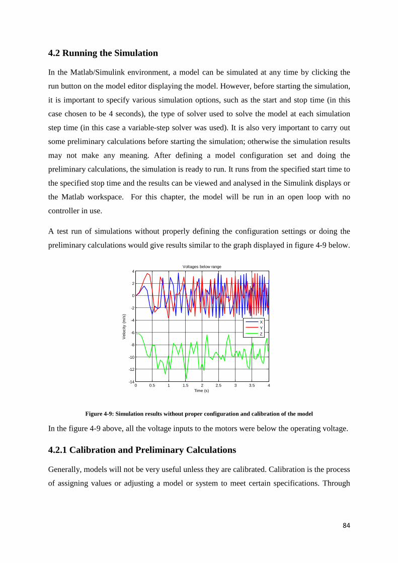
84
4.2 Running the Simulation
In the Matlab/Simulink environment, a model can be simulated at any time by clicking the
run button on the model editor displaying the model. However, before starting the simulation,
it is important to specify various simulation options, such as the start and stop time (in this
case chosen to be 4 seconds), the type of solver used to solve the model at each simulation
step time (in this case a variable-step solver was used). It is also very important to carry out
some preliminary calculations before starting the simulation; otherwise the simulation results
may not make any meaning. After defining a model configuration set and doing the
preliminary calculations, the simulation is ready to run. It runs from the specified start time to
the specified stop time and the results can be viewed and analysed in the Simulink displays or
the Matlab workspace. For this chapter, the model will be run in an open loop with no
controller in use.
A test run of simulations without properly defining the configuration settings or doing the
preliminary calculations would give results similar to the graph displayed in figure 4-9 below.
Figure 4-9: Simulation results without proper configuration and calibration of the model
In the figure 4-9 above, all the voltage inputs to the motors were below the operating voltage.
4.2.1 Calibration and Preliminary Calculations
Generally, models will not be very useful unless they are calibrated. Calibration is the process
of assigning values or adjusting a model or system to meet certain specifications. Through
0 0.5 1 1.5 2 2.5 3 3.5 4-14
-12
-10
-8
-6
-4
-2
0
2
4
Time (s)
Vel
ocity
(m/s
)
Voltages below range
XYZ
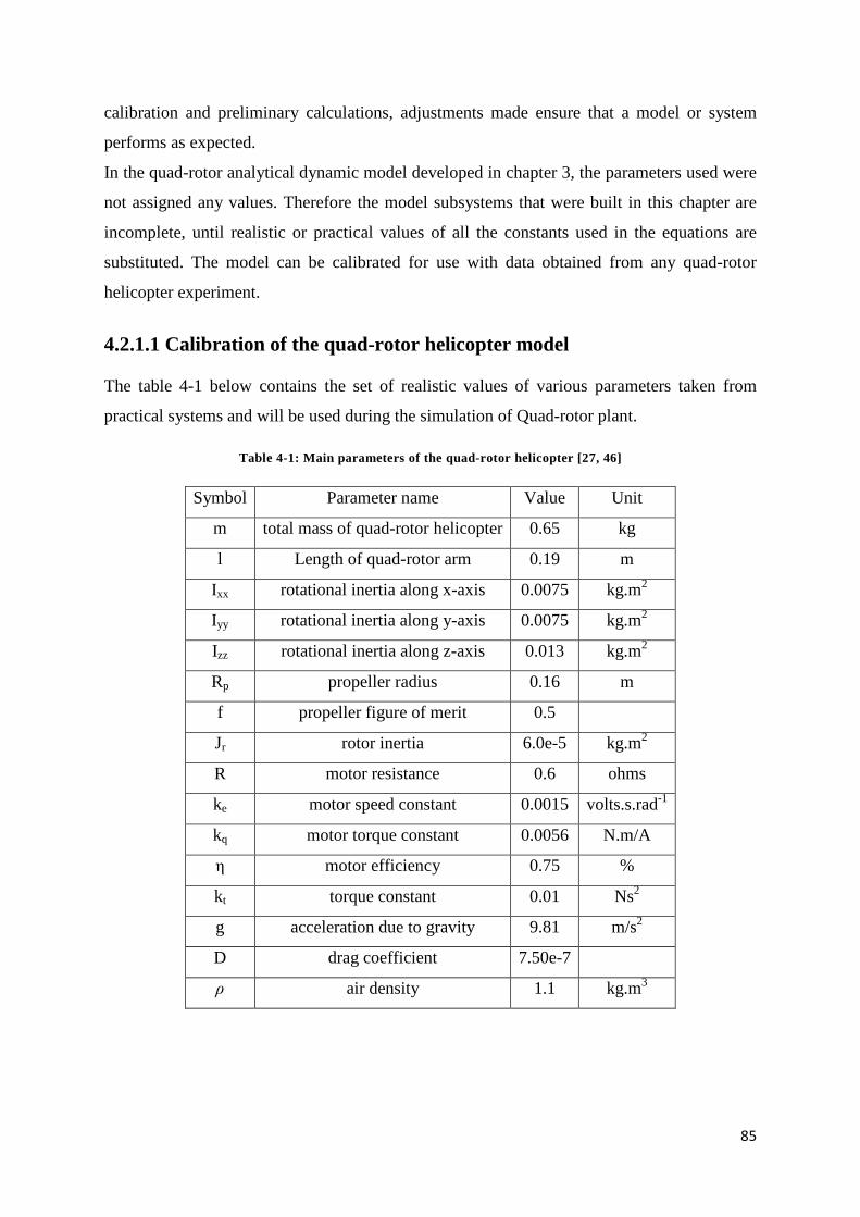
85
calibration and preliminary calculations, adjustments made ensure that a model or system
performs as expected.
In the quad-rotor analytical dynamic model developed in chapter 3, the parameters used were
not assigned any values. Therefore the model subsystems that were built in this chapter are
incomplete, until realistic or practical values of all the constants used in the equations are
substituted. The model can be calibrated for use with data obtained from any quad-rotor
helicopter experiment.
4.2.1.1 Calibration of the quad-rotor helicopter model
The table 4-1 below contains the set of realistic values of various parameters taken from
practical systems and will be used during the simulation of Quad-rotor plant.
Table 4-1: Main parameters of the quad-rotor helicopter [27, 46]
Symbol Parameter name Value Unit
m total mass of quad-rotor helicopter 0.65 kg
l Length of quad-rotor arm 0.19 m
Ixx rotational inertia along x-axis 0.0075 kg.m2
Iyy rotational inertia along y-axis 0.0075 kg.m2
Izz rotational inertia along z-axis 0.013 kg.m2
Rp propeller radius 0.16 m
f propeller figure of merit 0.5
Jr rotor inertia 6.0e-5 kg.m2
R motor resistance 0.6 ohms
ke motor speed constant 0.0015 volts.s.rad-1
kq motor torque constant 0.0056 N.m/A
η motor efficiency 0.75 %
kt torque constant 0.01 Ns2
g acceleration due to gravity 9.81 m/s2
D drag coefficient 7.50e-7
ρ air density 1.1 kg.m3

86
4.2.1.2 Calculation of operating point voltage and motor speed
An operating point has been chosen, in this case when the quad-rotor is hovering. This
implies that the vehicle’s x-y body plane is parallel to the x-y earth plane equivalent to a
situation when the vehicle’s roll, pitch and yaw angles together with their first and second
derivates (i.e. the angular velocities and accelerations) are all equal to zero. Also, there is no
movement in the x-, y- or z- directions, meaning that the linear velocities and accelerations
are all equal to zero. The operating point input voltage that corresponds to achieving the
situation described above can be calculated from the quad-rotor system equation 4-7, which
relates the voltage and the vertical acceleration. Here, all operating points are represented
with subscript ‘h’.
( )( ) gVVVVk
kfm
Azq
t −+++
=
••
ϕθηρ coscos2 24
23
22
21
2
With
=======Ω=Ω
Ω=Ω=========
•••••••••
•••
•••••••••
00
0
zzyyxx
h
ψϕθψϕθψϕθ
(4-8)
Substituting the values of all the constants from the calibration table 4-1 and the conditions
listed in equation 4-8 above, the following is obtained
( )( ) 81.90cos0cos0056.0
01.075.05.065.0
08042.01.120 24
23
22
21
2
−+++
××
××
= VVVV
( ) 81.9)44842.0)(27219.0(0 24
23
22
21 −+++= VVVV
( ) 81.912206.00 24
23
22
21 −+++×= VVVV
Here, it is assumed that all the motors behave in exactly the same way and the design of the
helicopter is symmetric; hence their voltage inputs at operating point are thought to be equal.
4321 VVVVVh ==== (4-9)
( ) 81.9412206.00 2 −×= hV

87
09333.20=hV
VoltsVh 48.4= (4-10)
Equation 4-10 gives the operating point voltage input for the motors of the quad-rotor
helicopter. For this voltage, we can find the speed with which the motors spin at the operating
point by substituting using the equation 4-1, which describes the relationship between the
motor speed and voltage input.
qe
q kRDk
kJRV
2Ω+Ω+
Ω=
•
At the operating point voltage hV , let the motor speed be hΩ
2
0056.000000075.060.00015.0
0056.06.000006.0
Ω
×
+Ω+Ω
×
=•
hV
20000804.00015.000643.048.4 Ω+Ω+Ω=•
201250.023328.073406.696 Ω−Ω−=Ω•
Since the motor speeds remain constant at hover, •
Ω =0 and on substituting we have the
following quadratic equation
001250.023328.073406.696 2 =Ω−Ω− (4-11)
Using the almighty formula for solving quadratic equations,
aacbbx
242 −±−
=
)01250.0(2]73406.696)01250.0(4[)23328.0()23328.0( 2
−××−×−−±−−
=Ωh
025.089112.3423328.0
−±
=Ωh

88
025.089112.3423328.0
−+
=Ωh Or 025.0
89112.3423328.0−
−=Ωh
sradh /61.245−=Ω Or sradh /94.226=Ω
By discarding the negative root of the quadratic equation, the speed at operating voltage is
sradh /94.226=Ω (4-12)
Figure 4-10 shows a graph of the motor speed versus time for the operating point voltage of
4.48 volts, confirming that the electric motor rises quickly to the operating point speed of
226.94 rad/s and remains there provided there is no voltage change.
Figure 4-10: Electric motor response to operating voltage step input
The motor voltage for each of the motors has to be at least the value of the operating point
voltage (4.48volts) to offset the weight of the helicopter. This leads to the helicopter just
lifting off the ground and hovering at a certain height. Outside that, the simulation results are
not valid as the motors may spin, but not have any effect on the helicopter model because
they do not generate enough lift to move it. Therefore, the operating point voltage serves as
the minimum voltage to be applied throughout this simulation process and the motors require
very little changes in voltages for control of the quad-rotor helicopter, because of its inherent
sensitivity to changes in rotor speeds.
0 0.5 1 1.5 2 2.5 3 3.5 40
50
100
150
200
250
Time (s)
Mot
or s
peed
(rad
/s)
Electric motor response

89
4.2.2 Hover
In the hover mode, it is assumed that the helicopter is at a height, far enough from the ground
such as to avoid the ground effect [a condition of improved performance encountered when
operating near (within 1/2 rotor diameter) of the ground. It is due to the interference of the
surface with the airflow pattern of the rotor system, and it is more pronounced the nearer the
ground is approached]. Here, all the propellers rotate at the same (hovering) speed to generate
a collective lift force that offsets the weight of the quad-rotor helicopter. As a consequence,
the quad-rotor neither climbs nor descends, it does not stall, roll, pitch or yaw and therefore
there is no horizontal movement in any direction. It stays at a fixed point in the air and does
not move from its position because there is a balance in all the forces and torques that are
acting on the vehicle. All simulations performed in this chapter were done while trying to
maintain a height of 0.92m as shown in figure 4-11 below.
Figure 4-11: Height reached at hover
As explained in the basic concepts of the quad-rotor helicopter (chapter 1), there are four
basic control actions, which allow the quad-rotor helicopter to reach a certain altitude and
attitude. Simulations have been run for each of the four basic control actions and results
displayed with analysis of the quad-rotor behaviour according to each of the commands.
4.2.3 Throttle (Vertical Motion)
This control action is realized by simultaneously increasing (or decreasing) all propeller
speeds by identical amounts. This implies that from an initial hover state, if the same amount
of voltage is added to the four motors simultaneously, the quad-rotor helicopter will heave
0 0.5 1 1.5 2 2.5 3 3.5 40
0.1
0.2
0.3
0.4
0.5
0.6
0.7
0.8
0.9
1
Time (s)
Z-P
ositi
on (m
)
Height reached at hover

90
(move vertically upwards), because of the collective vertical force generated by the four
propellers.
Fig 4-12 shows the height attained by the quad-rotor helicopter when an input of 4.6 volts is
given to each of the motors.
Figure 4-12: Height reached when each motor is given an input of 4.6volts
It is seen to reach a height of about 3.75m. This clearly shows that for very little voltage
changes, the motion of the quad-rotor helicopter is affected.
From the fig 4-13 below, it can be clearly seen that the upward velocity quickly increases and
then stops at a certain value because the voltage remains constant at that point.
Figure 4-13: Upward velocity of quad-rotor helicopter
0 0.5 1 1.5 2 2.5 3 3.5 40
0.5
1
1.5
2
2.5
3
3.5
4
Time (s)
Z-po
sitio
n (m
)Height reached at 4.6 volts
0 0.5 1 1.5 2 2.5 3 3.5 40
0.05
0.1
0.15
0.2
0.25
0.3
0.35
0.4
0.45
0.5
Time (s)
Vel
ocity
(m/s
)
Helicopter vertical velocity

91
Therefore the simultaneous increase to a certain value of the voltages in the four motors by
the same amount means that the collective vertical thrust generated by the four rotors
becomes greater than the weight of the helicopter and so the vehicle starts a vertical climb.
However, with an increase in the vertical speed, the thrust coefficient decreases, and so will
the collective vertical thrust, hence the total thrust equates the weight of the helicopter again
– defining a new point of equilibrium. Having reached that point of equilibrium, the
helicopter climbs at a steady speed, implying a zero upward acceleration, as also confirmed in
[2]. Figure 4-14 shows the total thrust generated at different motor speeds.
Figure 4-14: Total thrust generated at different motor speeds
The dependence of the collective vertical thrust on the vertical speed is also applicable to
situations when the helicopter is descending, but this time the collective vertical thrust
increases. Therefore, if the voltages are simultaneously decreased to a certain value by the
same amount, the helicopter will descend at increasing speeds until a limit value is reached.
It is worthy of note that, since z-axis points upwards, a negative velocity or acceleration,
simply means that the quad-rotor helicopter is descending, and a negative altitude means that
it is below the starting level.
4.2.4 Roll
The roll command is provided by simultaneously increasing (or decreasing) the left propeller
speed and decreasing (or increasing) the right propeller speed, while keeping the front and
rear propellers spinning at the same speed. With one rotor spinning faster than the rotor on
the opposite side, more lift will be generated on the side of the faster spinning rotor, therefore
230 240 250 260 270 280 290 300 3100
2
4
6
8
10
12
14
Motor speed (rad/s)
Forc
e (N
)
Total vertical thrust

92
the helicopter will tilt at a certain angle as shown in figure 4-15. This is because of the torque
created by the changes in lift forces with respect to the quad-rotor body x-axis.
Figure 4-15: Roll angle
While the front and rear motors were given a voltage supply of 4.5200 volts each (keeping
each of them at a speed of 227.9938 rad/s), the left motor had a voltage input of 4.5198 volts
(spinning at a speed of 227.9889 rad/s) and the right motor had an input of 4.5202 volts
(spinning at a speed of 227.9990 rad/s). The result as seen in the figure 4-15 is an angle of -
3.33 degrees. It is worthy of note that the – (minus) sign in the angle shows only the direction
of tilt and movement of the quad-rotor helicopter and does not in any way affect the
magnitude of the angle.
Figure 4-16 shows the position reached by the helicopter as a result of the roll angle created.
Figure 4-16: Y-displacement as a result of roll angle
0 0.5 1 1.5 2 2.5 3 3.5 4-3.5
-3
-2.5
-2
-1.5
-1
-0.5
0
Time (s)
Rol
l ang
le (d
eg)
Roll angle
0 0.5 1 1.5 2 2.5 3 3.5 4-0.1
0
0.1
0.2
0.3
0.4
0.5
0.6
0.7
0.8
Time (s)
Y-P
ositi
on (m
)
Y-Displacement
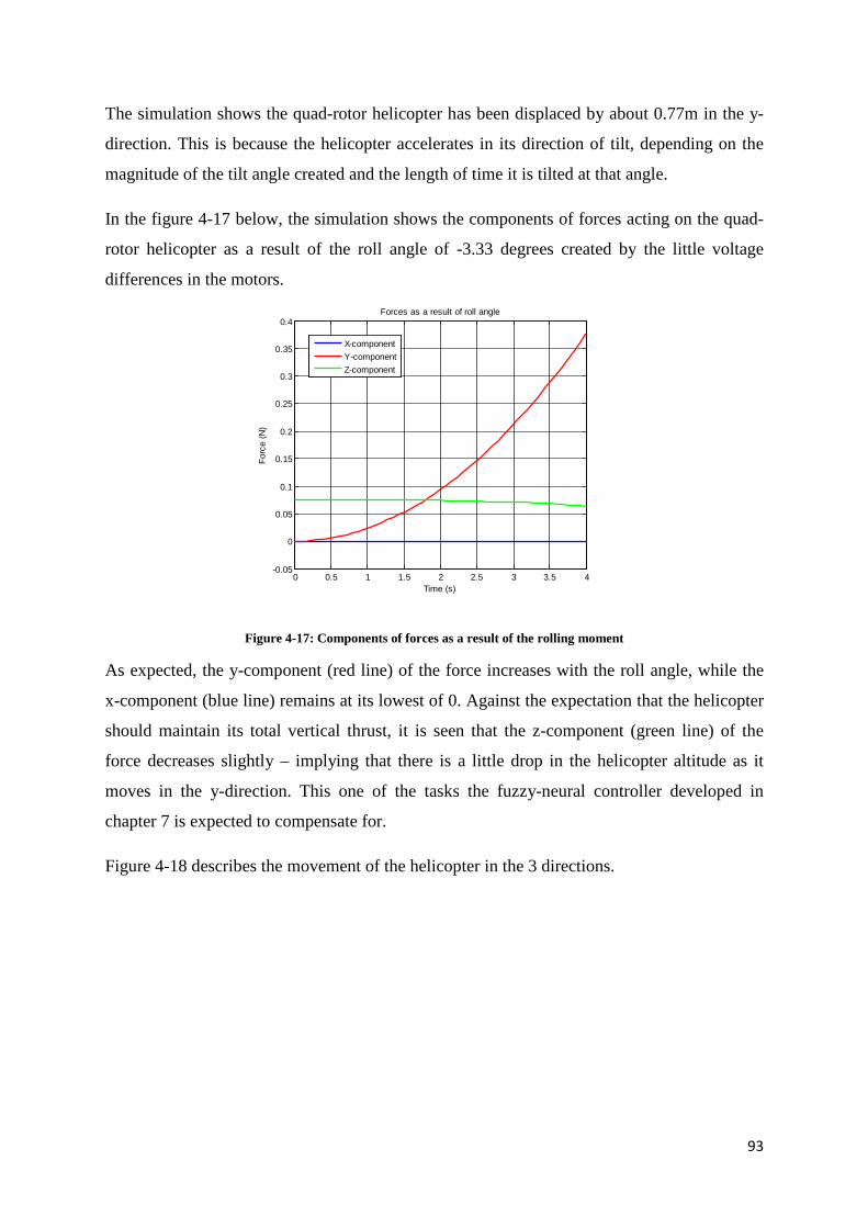
93
The simulation shows the quad-rotor helicopter has been displaced by about 0.77m in the y-
direction. This is because the helicopter accelerates in its direction of tilt, depending on the
magnitude of the tilt angle created and the length of time it is tilted at that angle.
In the figure 4-17 below, the simulation shows the components of forces acting on the quad-
rotor helicopter as a result of the roll angle of -3.33 degrees created by the little voltage
differences in the motors.
Figure 4-17: Components of forces as a result of the rolling moment
As expected, the y-component (red line) of the force increases with the roll angle, while the
x-component (blue line) remains at its lowest of 0. Against the expectation that the helicopter
should maintain its total vertical thrust, it is seen that the z-component (green line) of the
force decreases slightly – implying that there is a little drop in the helicopter altitude as it
moves in the y-direction. This one of the tasks the fuzzy-neural controller developed in
chapter 7 is expected to compensate for.
Figure 4-18 describes the movement of the helicopter in the 3 directions.
0 0.5 1 1.5 2 2.5 3 3.5 4-0.05
0
0.05
0.1
0.15
0.2
0.25
0.3
0.35
0.4
Time (s)
Forc
e (N
)
Forces as a result of roll angle
X-componentY-componentZ-component

94
Figure 4-18: Position reached when rolling
The graph in figure 4-11 shows the helicopter reaching a height of about 0.92m when all the
input voltages are 4.52 volts. Conversely figure 4-18 shows the quad-rotor helicopter
dropping to a height of 0.91m while moving to a position of about 0.77m in the y-direction,
corroborating the fact that a little bit of the total vertical thrust was lost during this
movement, despite the simultaneous increase (decrease) of the speeds of the left-right motor
pair. This could be as a result of some modelling assumptions, which the fuzzy-neural
controller is expected to deal with.
The figure 4-17 shows the components of forces acting on the quad-rotor helicopter as a
result of a particular roll angle (-3.33 degrees), where the y-component of the force increased
with the roll angle and the z-component decreased slightly. The graph in fig 4-19 shows
simulations carried out for different roll angles. While the y-component increased as the roll
angle got larger, the z-component continued to decrease – meaning that helicopter continued
to loose altitude with greater roll angles. The x-component (not shown in the graph) appeared
to be 0 or close to 0 for all the angles – implying that there was no movement in the x-
direction.
0 0.5 1 1.5 2 2.5 3 3.5 4-0.2
0
0.2
0.4
0.6
0.8
1
Time (s)
Pos
ition
(m)
Position reached when rolling
X-displacementY-displacementZ-displacement
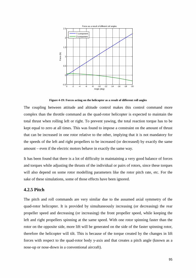
95
Figure 4-19: Forces acting on the helicopter as a result of different roll angles
The coupling between attitude and altitude control makes this control command more
complex than the throttle command as the quad-rotor helicopter is expected to maintain the
total thrust when rolling left or right. To prevent yawing, the total reaction torque has to be
kept equal to zero at all times. This was found to impose a constraint on the amount of thrust
that can be increased in one rotor relative to the other, implying that it is not mandatory for
the speeds of the left and right propellers to be increased (or decreased) by exactly the same
amount – even if the electric motors behave in exactly the same way.
It has been found that there is a lot of difficulty in maintaining a very good balance of forces
and torques while adjusting the thrusts of the individual or pairs of rotors, since these torques
will also depend on some rotor modelling parameters like the rotor pitch rate, etc. For the
sake of these simulations, some of those effects have been ignored.
4.2.5 Pitch
The pitch and roll commands are very similar due to the assumed axial symmetry of the
quad-rotor helicopter. It is provided by simultaneously increasing (or decreasing) the rear
propeller speed and decreasing (or increasing) the front propeller speed, while keeping the
left and right propellers spinning at the same speed. With one rotor spinning faster than the
rotor on the opposite side, more lift will be generated on the side of the faster spinning rotor,
therefore the helicopter will tilt. This is because of the torque created by the changes in lift
forces with respect to the quad-rotor body y-axis and that creates a pitch angle (known as a
nose-up or nose-down in a conventional aircraft).
-20-18-16-14-12-10-8-6-4-20-0.5
0
0.5
1
1.5
2
2.5
Angle (deg)
Forc
e (N
)
Force as a result of different roll angles
Y-componentZ-component
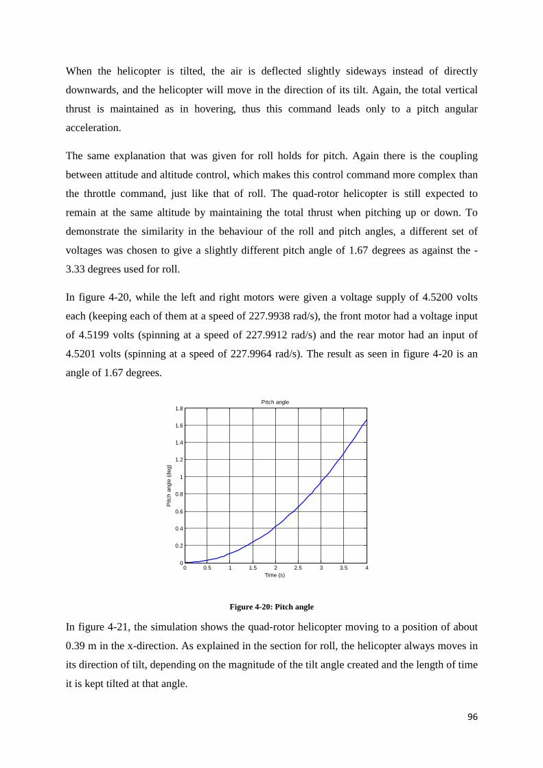
96
When the helicopter is tilted, the air is deflected slightly sideways instead of directly
downwards, and the helicopter will move in the direction of its tilt. Again, the total vertical
thrust is maintained as in hovering, thus this command leads only to a pitch angular
acceleration.
The same explanation that was given for roll holds for pitch. Again there is the coupling
between attitude and altitude control, which makes this control command more complex than
the throttle command, just like that of roll. The quad-rotor helicopter is still expected to
remain at the same altitude by maintaining the total thrust when pitching up or down. To
demonstrate the similarity in the behaviour of the roll and pitch angles, a different set of
voltages was chosen to give a slightly different pitch angle of 1.67 degrees as against the -
3.33 degrees used for roll.
In figure 4-20, while the left and right motors were given a voltage supply of 4.5200 volts
each (keeping each of them at a speed of 227.9938 rad/s), the front motor had a voltage input
of 4.5199 volts (spinning at a speed of 227.9912 rad/s) and the rear motor had an input of
4.5201 volts (spinning at a speed of 227.9964 rad/s). The result as seen in figure 4-20 is an
angle of 1.67 degrees.
Figure 4-20: Pitch angle
In figure 4-21, the simulation shows the quad-rotor helicopter moving to a position of about
0.39 m in the x-direction. As explained in the section for roll, the helicopter always moves in
its direction of tilt, depending on the magnitude of the tilt angle created and the length of time
it is kept tilted at that angle.
0 0.5 1 1.5 2 2.5 3 3.5 40
0.2
0.4
0.6
0.8
1
1.2
1.4
1.6
1.8
Time (s)
Pitc
h an
gle
(deg
)
Pitch angle

97
Figure 4-21: X-displacement as a result of pitch angle
In figure 4-22, the graph shows the components of forces acting on the quad-rotor helicopter
as a result of the pitch angle of 1.67 degrees. As seen in the roll angle simulation, the x-
component (blue line) of the force increases with the pitch angle, while the y-component (red
line) remains at its lowest of 0. Again it is clearly seen that the helicopter does not maintain
its total vertical thrust as the z-component (green line) of the force decreases slightly with a
movement in the x-direction as a result of the pitch angle.
Figure 4-22: Components of forces as a result of the pitching moment
Comparing again with the graph in figure 4-11, which shows the helicopter reaching a height
of 0.92m when all the input voltages are 4.52 volts, it is seen in figure 4-23 that the quad-
rotor helicopter drops to a height of 0.917m while moving to a position of about 0.39 m in the
0 0.5 1 1.5 2 2.5 3 3.5 40
0.05
0.1
0.15
0.2
0.25
0.3
0.35
0.4
Time (s)
X-p
ositi
on (m
)
X-Displacement

98
y-direction, confirming the fact that a little bit of the total vertical thrust was lost during this
movement, despite the simultaneous increase (decrease) of the speeds of the front-rear motor
pair.
Figure 4-23: Position reached when pitching
In figure 4-22, we see the components of forces acting on the quad-rotor helicopter as a result
of a pitch angle of 1.67 degrees. The x-component of the force increased with the pitch angle
(just like the y-component did with the roll angle in fig 4-17) and the z-component decreased
slightly. The graph in figure 4-24 shows simulations carried out for different pitch angles.
While the x-component increased as the pitch angle got larger, the z-component continued to
decrease – meaning that helicopter continued to loose altitude with greater pitch angles.
Figure 4-24: Forces acting on the helicopter as a result of different pitch angles
0 0.5 1 1.5 2 2.5 3 3.5 4-0.2
0
0.2
0.4
0.6
0.8
1
Time (s)
Pos
ition
(m)
Position reached when pitching
X-displacementY-displacementZ-displacement
0 2 4 6 8 10 12 14 16 18 20-0.5
0
0.5
1
1.5
2
2.5
Angle (deg)
Forc
e (N
)
Forces as a result of different pitch angles
X-componentZ-component

99
4.2.6 Yaw
This command simulates the rudder on a conventional fixed wing aircraft. It is realized by
simultaneously increasing (or decreasing) the front-rear propellers’ speed and decreasing (or
increasing) that of the left-right duo. As a result, there is a torque imbalance with respect to
the quad-rotor body z-axis and this makes the quad-rotor helicopter to pirouette about the
same axis in response to whichever direction the command is given.
While the left and right motors were given a voltage supply of 4.5150 volts each (keeping
each of them at a speed of 227.8627 rad/s), the front and rear motors each had a voltage input
of 4.525 volts (keeping each of them spinning at a speed of 228.1248 rad/s). The torque
imbalance results in a yaw angle of about 6.72 degrees as shown in figure 4-25.
Figure 4-25: Yaw angle
In the figure 4-26, the simulation shows the quad-rotor helicopter climbing to a height of
about 0.922m. This is as a result of a slight increase in the total vertical thrust occasioned by
spinning the front-rear motor pair a little faster than the left-right duo, which created the
torque imbalance on the helicopter. No horizontal movement was recorded because the pitch
and roll angles remained very close to 0 and could not cause any acceleration in the x or y
directions.
0 0.5 1 1.5 2 2.5 3 3.5 40
1
2
3
4
5
6
7
Time (s)
Yaw
ang
le (d
eg)
Yaw angle

100
Figure 4-26: Z-displacement
In the figure 4-27, the graph shows the components of forces acting on the quad-rotor
helicopter as a result of the yaw angle of 6.72 degrees. While the z-component (green line) of
the force increased slightly, the x and y components remained very close to 0 – implying the
helicopter only moved vertically upwards while changing heading by 6.72 degrees.
Figure 4-27: Components of forces as a result of the yawing moment
On comparing with the graph in figure 4-11, which shows the helicopter reaching a height of
0.92m when all the input voltages are 4.52 volts, it is seen in figure 4-28 that the quad-rotor
helicopter climbs to a height of 0.922m while yawing 6.72 degrees, confirming the fact that
there was a little increase in the total vertical thrust.
0 0.5 1 1.5 2 2.5 3 3.5 40
0.1
0.2
0.3
0.4
0.5
0.6
0.7
0.8
0.9
1
Time (s)
Z-P
ositi
on (m
)
Z-Displacement
0 0.5 1 1.5 2 2.5 3 3.5 40
0.01
0.02
0.03
0.04
0.05
0.06
0.07
0.08
Time (s)
Forc
e (N
)
Forces as a result of yaw angle
X-component
Z-component

101
Figure 4-28: Position reached when yawing
Figure 4-29, shows a slight but steady rise in the z-component of the force as the yaw angle
increases. Having to increase the speed of one pair while keeping the other pair constant is
responsible for this slight increase in the total vertical thrust.
Figure 4-29: Forces acting on the helicopter as a result of different yaw angles
This control is a little easier to achieve, because the inertia of the quad-rotor around the z-axis
is approximately double those of the x- and y- axes. Furthermore, there is no obvious cross-
coupling between the yaw and altitude controls. There is no translational motion since the
helicopter does not tilt in any direction and since the total vertical thrust is expected to be
maintained as in the hover state, there has to be a constraint on the amount of torque that can
be increased in a pair of rotors relative to the other. Normally, the rotor speed changes
required to achieve such control are very small, so it can be assumed that to maintain the total
0 0.5 1 1.5 2 2.5 3 3.5 40
0.1
0.2
0.3
0.4
0.5
0.6
0.7
0.8
0.9
1
Time (s)
Pos
ition
(m)
Position reached when yawing
X-displacementY-displacementZ-displacement
0 2 4 6 8 10 12 14 16 18 20
0.075
0.08
0.085
0.09
0.095
0.1
0.105
0.11
0.115
0.12
Angle (deg)
Forc
e (N
)
Force as a result of different yaw angles

102
thrust, the increase and decrease of the speeds of the motor pairs are done by the same
amounts.
4.3 Chapter Summary
The developed analytical model has been simulated in Matlab/Simulink software and the
dynamic behaviour of the quad-rotor assessed due to voltage changes. The main purpose of
this chapter was to analyse the results produced by the Simulink model, given different
voltage inputs. Previously known flight behaviours were confirmed, possible control
problems were identified and new flight behaviours were noted, preparatory to the design of
the controller.
Inevitably some effects have not been included in the model, and these effects could modify
the results that have been obtained here. The model can further be calibrated and linearized
for use on any quad-rotor helicopter, depending on the nature of the flight control problem.
Please see appendix F for more details on linearization.

103
CHAPTER 5
QUAD-ROTOR 3-D CAD MODEL AND COMPUTATIONAL FLUID
DYNAMICS (CFD) SIMULATION
This chapter presents details of CFD simulation and analysis of the quad-rotor helicopter. It
starts by showing how SolidWorks 2013 software is used to develop a 3-D CAD model of the
quad-rotor helicopter, with the same parameter values as that of the analytical dynamic model
developed in chapter 3 and simulated in chapter 4 of this thesis. Computational Fluid
Dynamics (CFD) as a computer based mathematical modelling tool is then used to simulate
and analyse the effects of wind flow patterns on the performance and control of the quad-
rotor helicopter.

104
5.0 Quad-rotor Helicopter CFD
Computational Fluid Dynamics (CFD) as a computer based mathematical modelling tool can
be considered as the combination of theory and experimentation in fluid flows. It is now
generally accepted and extensively used as a valid engineering tool in industry.
CFD computations are founded upon the fundamental governing equations of fluid dynamics
– the conservation of mass, momentum and energy. These equations combine to form the
Navier-Stokes equations, which are known to be a set of partial differential equations that
cannot be solved analytically except in a limited number of cases. Nevertheless, approximate
solutions can be obtained using discretisation methods that approximate the partial
differential equations by a set of algebraic equations. The most frequently used are the finite
volume method, the finite element method and the finite difference method. The resulting
algebraic equations relate to small sub-volumes within the flow, at a finite number of discrete
locations.
Any air-breathing propulsion system, be it a pure jet, an engine-propeller combination, an
engine-rotor combination, or a motor-rotor combination (like the quad-rotor helicopter),
derives its net thrust by adding momentum to a volume of air [95]. Therefore, the production
of thrust in helicopters is based solely on the action of the propeller. As the propeller rotates,
it causes the air around it to accelerate from one side to the other, which results in the
development of thrust in the opposite direction of the flow.
The rotor blades of the quad-rotor helicopter are responsible for three basic functions:
1. The generation of a vertical lifting force (thrust) in opposition to the aircraft weight.
2. The generation of a horizontal propulsive force for forward flight and sideways flight.
3. A means of generating forces and moments to control the attitude and altitude of the
helicopter.
The aerodynamics of the helicopter is one of the most challenging problems facing
aerodynamicists, but with the rapid increase in computational power and storage in recent
times, CFD simulation has turned out to be a realistic way of predicting the air flow around
the rotor blade. This certainly makes way for accurate prediction and understanding of the
aerodynamics of the entire quad-rotor helicopter [96].
The physics which governs fluids is relatively simple; the laws of motion and
thermodynamics with a little bit of chemistry. However, the solutions are very complex and

105
this makes analytical methods (pen and paper) largely unusable for industrial applications. A
common engineering approach to such complex dilemmas is to replace the problem with a
number of smaller less complex problems [97].
As the quad-rotor helicopter flies around, the fluid in which it is submerged (in this case air)
must move out of its way. The manner in which the air flows around it depends on its shape
as the flow could be smooth but more likely will contain vortices, shockwaves and other
disturbances as shown in figure 5-1.
Figure 5-1: Air flows around the quad-rotor helicopter in a CFD simulation
To model the behaviour of the fluid (air) the volume is split into many small sub-volumes,
called a mesh (or grid). A mesh can be simply the same sub-volume repeated throughout the
space or, more usually, it can be moulded around the helicopter CAD model as shown in
figure 5-2. Splitting the volume into sub-volumes is elegant in theory but hard in practice.
The art is to create a mesh with exactly the right sub-volumes – if the sub-volumes are too big
then the solution will have errors, if the volumes are too small then the calculation will take
too long.

106
Figure 5-2: CFD mesh diagram
The airflow is analysed by starting from an initial flow, which can be either a guess at the
solution or a specific initial condition. Using this initial flow the conservation equations are
used to predict the flow a short time later. A new prediction is then made from the newly
calculated flow. In this way the evolution of the airflow can be solved. In some situations
(mostly when flying indoors or even outdoors without a disturbance), flows around the rotor
blades of the helicopter are steady. For these steady flows, the process is repeated until the
solution doesn’t change from one time to the next, i.e. a convergence. The opposite of this is
when the flows around the rotor blades are unsteady. For these uneven flows, the solution
never settles down and CFD aims to track how the flow changes with time [63].
This explanation of using the conservation equations as a flow solver is a simplification; there
are other more complex solvers. However, these methods produce similar outputs and, more
importantly, CFD systems look the same to a user regardless of the solution technique.
Having obtained a flow solution, the user is presented with the flow at every point in the
mesh. This is a vast amount of data and not very useful on its own. The last phase of the CFD
process is to extract from these data the information that the user actually wants, in this case
the velocities, accelerations and forces acting on the quad-rotor helicopter.

107
The flowchart in figure 5-3 shows the three major stages involved in using CFD to simulate a
quad-rotor helicopter.
Figure 5-3: CFD process flow
a) Computer Aided Design (CAD) – using software to build a model of the quad-rotor
helicopter and to represent it in the flow domain. It entails the following:
Approximation of the geometry – the geometry of the quad-rotor needs to be
approximated by a geometric CAD type model. More accurate results are obtained
from a model geometry that more closely represents the actual geometry.
Creation of the numerical grid within the geometrical model – to identify the discrete,
finite locations at which the variables are to be calculated, the geometry is divided
into a finite number of cells that make up the numerical grid. Before doing this, it is
necessary to identify the physical flow phenomena expected (turbulence,
compressible flow, shocks, multiphase flow, mixing, etc.) so that the grid generated is
suitable to capture these phenomena.
Selection of models and modelling parameters – once the geometry and grid have
been established, the mathematical models and parameters for those phenomena are
then selected and boundary conditions defined throughout the computational domain.

108
b) CFD Flow Solver – obtaining a flow solution by running a flow-solver to simulate the
quad-rotor helicopter’s fluid environment using the grid for flow conditions specified by
the researcher. It involves:
Calculation of the variable values – discretisation yields a large number of algebraic
equations (one set for each cell). These equations are then generally solved using an
iterative method, starting with a first guess value for all variables and completing a
computational cycle. Error or residual values are computed from the discretised
equations and the calculations repeated many times, reducing the residual values, until
a sufficiently converged solution is judged to have been reached.
Determination of a sufficiently converged solution – the final stage in the solution
process is to determine when the solution has reached a sufficient level of
convergence. When the sum of the residual values around the system becomes
sufficiently small, the calculations are stopped and the solution is considered
converged. A further check is that additional iterations produce negligible changes in
the variable values.
c) Data Analysis, Presentation and Verification – analysing the flow data from the results of
the flow-solver and modifying the model until a design satisfaction is achieved. It
involves:
Post Processing – once a converged solution has been calculated, the results can be
presented as numerical values or pictures, such as velocity vectors and contours of
constant values (e.g. pressure or velocity).
Solution Verification and Validation – once the solution process is complete, each
solution should be verified and validated. If this cannot be completed successfully, re-
simulation may be required, with different assumptions and / or improvements to the
grid, models and boundary conditions used.
5.1 Quad-rotor 3-D CAD Model
Building such a model commonly begins with a 2-D draft of the helicopter parts. The draft
comprises of geometry such as points, lines, arcs, conics and etc. Measurements are then
added to the draft to outline the size and positions of the geometry. The relationships between
the parts such as their intersections at tangents, their being perpendicular or parallel or
concentric are normally used to define attributes. With its parametric nature, SolidWorks
allows the measurements and relations to drive the geometry. The measurements in the draft

109
can be organized individually, or by relationships to other parameters inside or outside of the
draft [98]. Table 5-1 shows the quad-rotor helicopter parts designed using SolidWorks.
Table 5-1: Quad-rotor UAV CAD parts
Part Description Quantity Mass (g)
BLDC motor 4 40 x 4 = 160.00
Arm 4 35 x 4 = 140.00
Propeller 4 12.60 x 4 = 50.40
Central Hub
(with all electronics and battery)
1 253.30
Landing gear 2 15.20 x 2 = 30.40
Payload (camera) 1 15.90
Total weight 650.00
Having carefully designed the different components based on the same parameter values as
that of the analytical dynamic Matlab/Simulink model in chapter 4, they were assembled to
form the quad-rotor helicopter model shown in figure 5-4 below, with details given in
appendix B of this thesis.

110
Figure 5-4: SolidWorks 3-D model of the quad-rotor helicopter
5.2 CFD Flow Solver
The flow-solver used in this research work is SolidWorks Flow Simulation 2013. Flow
Simulation is a fluid flow and heat transfer analysis software fully integrated into
SolidWorks. It simulates the quad-rotor helicopter’s 3-D prototype in its working fluid
environment, thereby giving predictions of the effects of the fluid flow on the helicopter
prototype and the helicopter's effects on the fluid flow around it.
The outstanding feature of Flow Simulation is its intuitively clear and comfortable interface
including a pre-processor for defining the type of analysis, specifying data and boundary
conditions for the calculation (with an Engineering Database on substance properties); co-
processor for monitoring and controlling the computation process and checking the
convergence where necessary; postprocessor for visualizing the results obtained [99].
Figure 5-5: Flow-solver dialogue box

111
The main objective of conducting the CFD simulation in this research is to simulate the
effects of the external environment on the flow patterns of the quad-rotor helicopter within a
computational domain.
The computational domain is a rectangular parallelepiped for both the 3D analysis and 2D
analysis. Its boundaries are parallel to the Global Coordinate System planes as shown in
figure 5-6. Sometimes overlooked, the computational domain is one of the many important
factors that influence the validity and accuracy of CFD simulation results. The use of
different computational domains has turned out varied results, even for the same set of rotor
speeds. Therefore, the choice of computational domain could significantly affect the results
of such simulations.
Figure 5-6: Computational domain of CFD simulation
In many cases, the advantage of working on a rectangular computational domain, with a
uniform rectangular grid, compensatory to the more complicated form of the equation being
used. The problem is finding the coordinate transformation, which maps the physical domain
into the needed computational domain, such that the uniform rectangular grid in the
computational domain corresponds to a non-uniform curvilinear grid in the physical domain
[100].
Due to specified conditions, the characteristics of the fluid flow may have large variations in
some regions in the physical space. In these regions, a refinement of the grid should be very
useful, as it yields increased accuracy, without a supplementary computing effort.

112
Figure 5-7 shows the distribution of air around the rotors of the quad-rotor helicopter as they
spin and add momentum to the volume of air they are immersed in. The lift force would
normally rise perpendicularly to the air stream caused by Bernoulli Effect. This causes a
lower pressure on top of the rotor blade, compared with the pressure at the bottom. The
curvature on the top of the blade leads to a higher stream velocity than at the bottom and
hence a lower pressure [101].
Figure 5-7: Air distribution around the rotors during simulation
A close observation shows that near the ends of the rotating blades, there is some turbulence
and the airflow tends to move upwards. Interactions between the wakes produced by the
rotors and the fuselage, and also between individual rotors can also be observed. The
cumulative air flow tends to go upwards, compensating the lift force.
5.3 Analysis of CFD results
In the analytical dynamic Matlab/Simulink model in chapter 4, voltage applied to the DC-
motor model results in angular acceleration; the same sets of angular accelerations obtained
from the Matlab/Simulink model were used in the flow simulation in this chapter, as shown
in figure 5-8. The accelerations and forces produced as a result of each of the four basic
commands of throttle, roll pitch and yaw were recorded and analysed for situations with and
without wind disturbance. In the windy situations, the quad-rotor helicopter was exposed to
wind speeds of different magnitudes and directions.
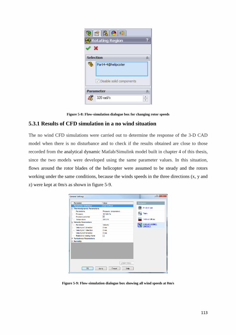
113
Figure 5-8: Flow-simulation dialogue box for changing rotor speeds
5.3.1 Results of CFD simulation in a no wind situation
The no wind CFD simulations were carried out to determine the response of the 3-D CAD
model when there is no disturbance and to check if the results obtained are close to those
recorded from the analytical dynamic Matlab/Simulink model built in chapter 4 of this thesis,
since the two models were developed using the same parameter values. In this situation,
flows around the rotor blades of the helicopter were assumed to be steady and the rotors
working under the same conditions, because the winds speeds in the three directions (x, y and
z) were kept at 0m/s as shown in figure 5-9.
Figure 5-9: Flow-simulation dialogue box showing all wind speeds at 0m/s

114
A comparison of the results obtained from the analytical dynamic Matlab/Simulink model,
the 3-D Solidworks model and real flight experiment data is done in chapter 6 of this thesis,
where a compensation architecture is also developed.
5.3.1.1 Throttle
As explained in chapter 1, spinning the four rotors at the same speed would either increase or
decrease the altitude of the helicopter, thereby generating a collective vertical force from the
four propellers. The upward velocity of the quad-rotor helicopter and the collective lift force
at different rotor speeds from the flow simulation are represented in figures 5-10 and 5-11
below.
Figure 5-10: Upward velocity of quad-rotor helicopter
Again the figure shows the upward velocity rising and then stops at about 0.41m/s because
the motor speeds remain constant.
It can be seen from figure 5-11 that as noted in the Matlab/Simulink model, the collective
vertical thrust increases as the motor speeds increase.
0 0.5 1 1.5 2 2.5 3 3.5 40
0.05
0.1
0.15
0.2
0.25
0.3
0.35
0.4
0.45
Time (s)
Vel
ocity
(m/s
)
Helicopter vertical velocity

115
Figure 5-11: Total thrust generated at different motor speeds
5.3.1.2 Roll
As stated earlier, differential thrust between the left and right rotors provides the roll torque.
The total vertical thrust is expected to be maintained as in hovering. The forces produced at
different tilt angles are shown in figure 5-12 below.
Figure 5-12: Forces acting on the helicopter as a result of different roll angles
While the front and rear motors were kept spinning at a speed of 227.9938 rad/s, the left
motor was spinning at a speed of 227.9889 rad/s and the right motor was spinning at a speed
of 227.9990 rad/s. This is the same set of motor speeds that created a roll angle of -3.33
degrees in the Matlab/Simulink model (figure 4-14 of chapter 4).
230 240 250 260 270 280 290 300 3100
2
4
6
8
10
12
14
Motor speed (rad/s)
Forc
e (N
)
Total vertical thrust
-20-18-16-14-12-10-8-6-4-200
0.5
1
1.5
2
2.5
Angle (deg)
Forc
e (N
)
Force as a result of different roll angles
Y-componentZ-component

116
In the figure 5-13, the CFD simulation shows a very similar behaviour with the
Matlab/Simulink model. The components of forces acting on the quad-rotor helicopter were
not exactly the same for the two models; they were a little bit lower but not too far apart. As
expected, the y-component (red line) of the force increases, while the z-component (green
line) of the force decreased slightly, the CFD simulation seemed better at maintaining the
total vertical thrust of the helicopter.
Figure 5-13: Components of forces as a result of the roll moment
Despite the minor discrepancies in the magnitude of forces acting on the vehicle in the two
models, the results obtained show that the two models are very similar, having being built
using the same parameters.
5.3.1.3 Pitch
The differential thrust between the front and rear rotors provides the pitch torque. The total
vertical thrust is expected to be maintained as in hovering. The forces produced at different
tilt angles are shown in figure 5-14 below.
0 0.5 1 1.5 2 2.5 3 3.5 4-0.05
0
0.05
0.1
0.15
0.2
0.25
0.3
0.35
0.4
Time (s)
Forc
e (N
)
Forces as a result of roll angle
X-componentY-componentZ-component

117
Figure 5-14: Forces acting on the helicopter as a result of different pitch angles
In the figure 5-15 below, the graph shows the components of forces acting on the quad-rotor
helicopter as a result of the same motor speeds that produced a pitch angle of 1.67 degrees in
the Matlab/Simulink model in figure 4-20 of chapter 4.
In this case, the left and right motors were spun at a speed of 227.9938 rad/s each, the front
motor was spun at a speed of 227.9912 rad/s and the rear motor at a speed of 227.9964 rad/s.
Figure 5-15: Components of forces as a result of the pitching moment
5.3.1.4 Yaw
Differential torque between the pairs of counter-rotating rotors provides the yaw torque. The
torque imbalance with respect to the z-axis makes the quad-rotor turn about the same axis. In
0 2 4 6 8 10 12 14 16 18 200
0.5
1
1.5
2
2.5
Angle (deg)
Forc
e (N
)
Force as a result of different pitch angles
X-componentZ-component
0 0.5 1 1.5 2 2.5 3 3.5 4-0.02
0
0.02
0.04
0.06
0.08
0.1
0.12
0.14
0.16
0.18
Time (s)
Forc
e (N
)
Forces as a result of pitch angle
X-componentY-componentZ-component
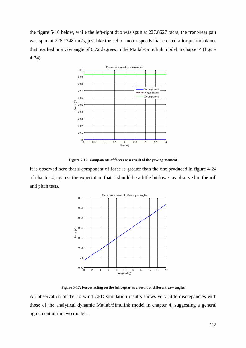
118
the figure 5-16 below, while the left-right duo was spun at 227.8627 rad/s, the front-rear pair
was spun at 228.1248 rad/s, just like the set of motor speeds that created a torque imbalance
that resulted in a yaw angle of 6.72 degrees in the Matlab/Simulink model in chapter 4 (figure
4-24).
Figure 5-16: Components of forces as a result of the yawing moment
It is observed here that z-component of force is greater than the one produced in figure 4-24
of chapter 4, against the expectation that it should be a little bit lower as observed in the roll
and pitch tests.
Figure 5-17: Forces acting on the helicopter as a result of different yaw angles
An observation of the no wind CFD simulation results shows very little discrepancies with
those of the analytical dynamic Matlab/Simulink model in chapter 4, suggesting a general
agreement of the two models.
0 0.5 1 1.5 2 2.5 3 3.5 40
0.01
0.02
0.03
0.04
0.05
0.06
0.07
0.08
0.09
0.1
Time (s)
Forc
e (N
)
Forces as a result of a yaw angle
X-componentY-componentZ-component
0 2 4 6 8 10 12 14 16 18 200.09
0.1
0.11
0.12
0.13
0.14
0.15
0.16
Angle (deg)
Forces as a result of different yaw angles
Forc
e (N
)

119
There are discrepancies because the computational fluid dynamics simulation considers some
of factors/conditions (such as drag and some modelling assumptions) ignored in the
Matlab/Simulink model, thereby providing a situation closer to actual flight experiments.
Despite the general agreement, the need for a verification and validation of the two models
with data obtained from real flight experiments as carried out in chapter 6 cannot be
extravagant.
5.3.2 Results of CFD simulation in windy situations
Wind speed and direction play important roles in flying any aircraft. The wind that flows
opposite to the flight path of the quad-rotor helicopter (headwind) slams the front of the
quad-rotor and slows it down, while a flow from the back (tailwind) forces the quad-rotor in
the direction of flight, increasing its speed. There could also be crosswinds that blow from the
sides, across the flight path and they are equally dangerous to the quad-rotor. These
conditions can lead to loss of control, deviation from the planned path or even a crash;
depending on the magnitude of the winds.
In this simulation, the quad-rotor helicopter experiences unsteady flows around its rotor
blades, with winds speeds of different magnitudes ranging from 0-15m/s in the three
directions (x, y and z) at different times as shown in the dialogue box in figure 5-18. The flow
data obtained here were very useful in the design and training of the controller in chapter 7,
since the quad-rotor is expected to fly through a series of complex weather conditions.
Figure 5-18: Dialogue box showing how the different wind speeds were set

120
In this situation, the rotors of the helicopter are working under different conditions, because
of the varying wind speeds and the non-uniformity of the flow of air around them. This is
expected to create some extra aerodynamic moments over the airframe.
For the control system to ensure that it keeps to the planned path in the presence of a
disturbance, a quad-rotor tilt angle must be created to compensate the drag force with a
horizontal component of the collective thrust force generated by the rotors, with stronger
winds requiring larger tilt angles.
With SolidWorks Flow Simulation, it is very easy to calculate fluid forces and understand the
impact of air flows on the performance and control of the quad-rotor helicopter as shown in
figures 5-19 below and 5-20.
Figure 5-19: Calculating the effect of wind disturbance on the quad-rotor helicopter
Based on the results obtained from the flow-solver, the effects of the vertical and horizontal
wind flows on the quad-rotor helicopter are summarised and discussed next.
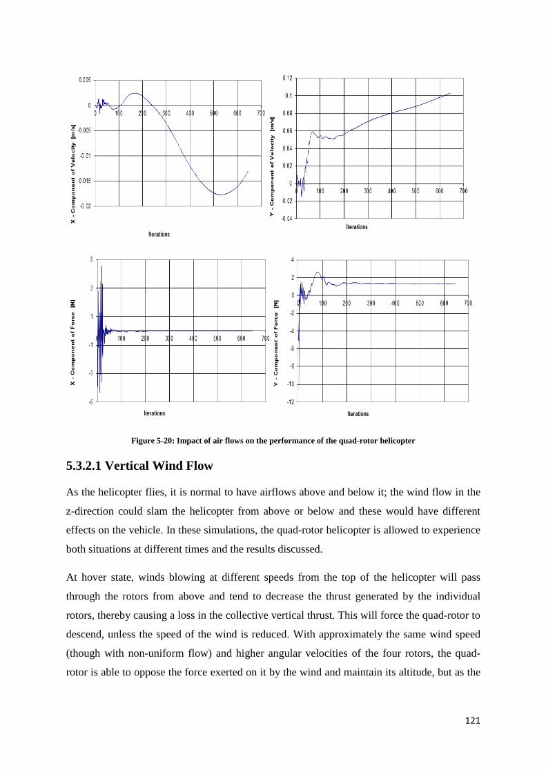
121
Figure 5-20: Impact of air flows on the performance of the quad-rotor helicopter
5.3.2.1 Vertical Wind Flow
As the helicopter flies, it is normal to have airflows above and below it; the wind flow in the
z-direction could slam the helicopter from above or below and these would have different
effects on the vehicle. In these simulations, the quad-rotor helicopter is allowed to experience
both situations at different times and the results discussed.
At hover state, winds blowing at different speeds from the top of the helicopter will pass
through the rotors from above and tend to decrease the thrust generated by the individual
rotors, thereby causing a loss in the collective vertical thrust. This will force the quad-rotor to
descend, unless the speed of the wind is reduced. With approximately the same wind speed
(though with non-uniform flow) and higher angular velocities of the four rotors, the quad-
rotor is able to oppose the force exerted on it by the wind and maintain its altitude, but as the

122
force exerted by the wind overcomes the collective thrust generated by the rotors, the
helicopter is always forced to descend.
The curves in figure 5-21 show a continuous reduction in the collective vertical thrust as the
wind speed increases without a corresponding change in the motor speeds.
Since the air flow and distribution is not uniform, there is a possibility that the quad-rotor will
either pitch or roll and move horizontally, even when a vertical movement is expected.
Figure 5-21: Total vertical thrust in downward flow of wind
The exact opposite would happen if the wind blew from below the helicopter as shown in
figure 5-22 below. The air will pass through the rotor blades from below and tend to increase
the collective vertical thrust generated by the rotors, leading to the quad-rotor ascending to a
certain height, only to stabilize when the wind or rotor speeds are reduced.
Figure 5-22: Total vertical thrust in upward flow of wind
230 240 250 260 270 280 290 300 3100
2
4
6
8
10
12
14
Motor speed (rad/s)
Forc
e (N
)
Total vertical thrust
Thrust at 0m/sThrust at 5m/sThrust at 10m/sThrust at 15m/s
230 240 250 260 270 280 290 300 3100
5
10
15
20
25
Forc
e (N
)
Motor speed (rad/s)
Total vertical thrust
Thrust at 0m/sThrust at 5m/sThrust at 10m/sThrust at 15m/s

123
5.3.2.2 Horizontal Wind Flow
The horizontal wind velocity normally has a crosswind component and a headwind/tailwind
component, which affect its speed relative to the ground. When the quad-rotor helicopter
experiences such a flow of wind around it, there certainly will be unwanted moments in
addition to other possible effects that act due to the fact that the flight conditions are much
more unstable. The quad-rotor helicopter is likely to depart from the state of equilibrium in
flight, leading to a possible loss of control.
In these simulations, the quad-rotor helicopter was exposed to headwinds, tailwinds and
crosswinds of different magnitudes as depicted in figure 5-23.
Figure 5-23: Quad-rotor experiencing cross winds in simulation
a) Headwind
In a headwind situation, the effect of the wind slamming the front of the quad-rotor helicopter
is seen from the curves in figures 5-24. The combined effect of the headwind and the
helicopter’s speed and forces always produces a resultant speed or force that is lower than the
one the helicopter had before it encountered the wind. There could also be a change in
direction of flight as suggested by the y-component (red line), depending on the direction and
magnitude of the wind.

124
Figure 5-24: Forces acting on the helicopter in a headwind
Stronger winds have a greater reduction effect on the quad-rotor’s speed and forces as
depicted in figure 5-25. Also notice that as the winds get stronger (red and light blue lines at
10m/s and 15m/s respectively), the quad-rotor seems to pitch violently as it struggles to stay
in flight.
Figure 5-25: Forces acting on the helicopter in a headwind at different tilt angles
b) Tailwind
Naturally, a tailwind is expected to increase the quad-rotor speed and forces in the direction
of flight as shown in figure 5-26 below. The effect of a tailwind on the forces acting on the
quad-rotor helicopter may not be the exact opposite of the curves in figure 5-25 above as the
effects of a headwind cannot be overcome by a tailwind of the same magnitude. Figure 5-26
shows increasing components of the x and y forces (blue and red lines) from 1-3 seconds of
the simulation, while the z-component experiences a little decrease. However, after 3 seconds
0 0.5 1 1.5 2 2.5 3 3.5 4-0.2
-0.15
-0.1
-0.05
0
0.05
0.1
0.15
Time (s)
Forc
e (N
)
Forces as a result of pitch angle in a headwind
X-componentY-componentZ-component
0 2 4 6 8 10 12 14 16 18 200
0.5
1
1.5
2
2.5
Angle (deg)
Forc
e (N
)
Quad-rotor forces in a headwind
X-component of force at wind 0m/sX-component of force at wind 5m/sX-component of force at wind 10m/sX-component of force at wind 15m/s

125
the y-component (red line) begins to decrease because of the fact that a tailwind would have a
greater effect on the pitch angle/moments of the quad-rotor helicopter and also the non-
uniform flow around it.
Figure 5-26: Quad-rotor forces in a tailwind
c) Crosswind
A crosswind would normally create an in-plane force that acts on the vehicle and tends to
create a moment that makes the quad-rotor helicopter tilt. The instant the quad-rotor starts to
tilt, it accelerates in its direction of tilt. However, too much of a tilt would make the quad-
rotor to start loosing equilibrium, thereby leading to a possible oscillation and loss of control
of the whole vehicle. Only a timely and accurate re-arrangement of the motor speeds can
maintain that equilibrium and keep it in the planned path.
As shown in figure 5-27 below, the wind blows in the direction of tilt of the helicopter. The
y-component (red line) of force increases with the crosswind, but since the flow is non-
uniform, there is a fluctuation in the x-component (blue line) of force, while the z-component
(green line) decreases. This clearly suggests instability in the vehicle because of the
disturbance.
0 0.5 1 1.5 2 2.5 3 3.5 4-0.05
0
0.05
0.1
0.15
0.2
0.25
0.3
Time (s)
Forc
e (N
)
Forces as a result of pitch angle in a tailwind
X-componentY-componentZ-component

126
Figure 5-27: Quad-rotor forces in a crosswind blowing in the direction of tilt of the helicopter
When the wind blows against the direction of tilt of the helicopter as shown in figure 5-28
below, the forces generally decrease. Notably, the x-component (blue line) of force reduces to
the negative, implying that the helicopter moved in the negative x-direction. Such simulations
would have been much easier if the winds hit the quad-rotor helicopter directly in front, at the
back or from the sides. However, the curves clearly indicate the result of an uneven
distribution of the force of the wind on the quad-rotor, making the problem of control even
more complex.
Figure 5-28: Quad-rotor forces in a crosswind blowing against the direction of tilt of the helicopter
Figure 5-29 shows the major forces acting on the quad-rotor in a crosswind. An increase in
the wind speed records an increase in the force if the wind is blowing in the direction of
movement of the helicopter. Note that from 10m/s (red line), the force curve begins to
0 0.5 1 1.5 2 2.5 3 3.5 4-0.1
0
0.1
0.2
0.3
0.4
0.5
0.6
Time (s)
Forc
e (N
)
Forces as a result of roll angle in a crosswind
X-componentY-componentZ-component
0 0.5 1 1.5 2 2.5 3 3.5 4-0.15
-0.1
-0.05
0
0.05
0.1
0.15
0.2
0.25
0.3
0.35
Time (s)
Forc
e (N
)
Forces as a result of roll angle in a crosswind
X-componentY-componentZ-component

127
oscillate, suggesting that the helicopter could be loosing equilibrium and possibly veering off
the planned path. A further increase in the wind speed could even see the quad-rotor
helicopter flip upside down and crash, if there is no adjustment made to the rotor speeds in
good time. The direction of movement or behaviour of the quad-rotor helicopter can be
difficult to predict if the wind is allowed to blow it off course.
Figure 5-29: Forces acting on the helicopter in a crosswind at different angles of tilt
5.4 Chapter Summary
CFD studies provide meaningful insight into the impact of fluid flow, enabling Engineers to
address problems early, reduce the need for costly prototypes, and eliminate rework.
A 3-D Solidworks model was also developed with the same parameter values as that of the
model developed in Matlab/Simulink. CFD was used to simulate and analyse the effects of
the external environment/disturbances on the flow patterns of the quad-rotor helicopter within
a given computational domain.
The helicopter stability and control analysis requires a very large number of CFD simulations
to determine appropriate forcing parameters within the expected range of motion. Typically,
the time accurate CFD simulations start from a steady state solution and are iterated in
pseudo time within each physical time step using a dual-time stepping scheme.
This chapter investigated the use of a 3-D Solidworks model that significantly reduced the
CFD simulation time required to create a full aerodynamics database, making it possible to
accurately model the quad-rotor static and dynamic characteristics from a limited number of
time-accurate CFD simulations, preparatory to the development of a robust adaptive
controller for the helicopter.
-20-18-16-14-12-10-8-6-4-200
0.5
1
1.5
2
2.5
3
3.5
4
Angle (deg)
Forc
e (N
)Quad-rotor forces in a crosswind
Y-component of force at wind 0m/sY-component of force at wind 5m/sY-component of force at wind 10m/sY-component of force at wind 15m/s

128
CHAPTER 6
VALIDATION OF MODELS WITH FLIGHT EXPERIMENT DATA
This chapter affords details of the verification, validation and equipment used to acquire real
flight test data in order to determine the credibility of the two models developed in chapters 4
and 5 of this thesis. Results of simulations performed with the two models are compared with
results from real flight experiments performed at University of Essex Robot Arena. An
artificial neural network function approximation tool, is trained with real flight experiment
data and used to correct the errors found in the two models.

129
6.0 Verification and Validation
There has been an increasing demand for dependable predictions of complex processes
encompassing, where possible, accurate predictions of full behaviours of non-linear dynamic
systems. This requirement is driven by the need for scientifically informed assessments in
support of very important judgements that affect humanity, including fault-tolerant and safety
critical systems, global warming, national security, health and transport.
Three possible methods are normally used for the prediction and analysis of the behaviours of
such systems: conducting experiments (real flight situations in the case of the quad-rotor
helicopter), theoretical analysis and computational or simulation methods. Results of
experiments are most reliable, but could be expensive and difficult to obtain. Theoretical
analysis has its confines, because equations that describe the system could be complex and
probably be solved for very simple known cases. The most viable method is to carry out
computer-based simulations to produce quantitative, predictive information about such
complex systems, just as has been done in chapters 4 and 5 of this thesis.
Generally, simulation models are inexact imitations of real-world systems and they never
accurately imitate the real-world system. Due to this fact, inaccuracies can pose very high
risks. It is therefore vital that simulation results have a high level of confidence. Verification
and validation of the simulation models using data obtained from actual experiments must be
done with the ultimate goal of producing an accurate and credible model as depicted in the
flowchart in figure 6-1 below.
Figure 6-1: Verification and validation process flow

130
In this chapter, results of simulations performed with the analytical Matlab/Simulink model
of the quad-rotor helicopter built in chapter 4 and those obtained using CFD on a 3-D
Solidworks model of the same helicopter in chapter 5 are compared with results of real flight
experiments performed at University of Essex Robot Arena. This ensures that any modelling
and simulation errors discovered are fixed. This also helps in deciding whether the simulation
models and results are realistic enough to be used for the quad-rotor fuzzy-neural controller
development.
6.1 Flight Experiments with the Quad-rotor helicopter
Quad-rotor flight experiments were conducted at the University of Essex to verify and
validate the two models developed in this thesis. The Essex Robotic Arena is an advanced
mobile robot research facility featuring a 100 square metre powered floor and real-time 3-D
VICON motion tracking system. It also boasts of a data logging system, which allows the
automatic logging of robot behaviour for subsequent analysis.
6.1.1 Experimental Set-up in the Robot Arena
The hardware set-up used for flight experiments as described in [102] is depicted in figure 6-
2 below and explained in subsections that follow.
Figure 6-2: Hardware set-up for flight experiments

131
a) Interface and Controller Computers
This is needed in the setup to run the algorithms for the behaviours and the controls. The
Workstation software takes information captured by the VICON hardware and combines it
with calibration data and a set of other parameters to create 3-D positions for each marker in
the capture volume. The positions are calculated frame-by-frame and combined to create a
complete set of trajectories of the markers positions throughout the time span of the
experiment. This would then open a USB port on the computer and send the required control
values to the USB to Serial Converter based on the information obtained from the VICON
video system.
b) USB to Serial Converter
This receives the control values from the computer and converts them to serial
communications protocol format. It then transmits the control values over a wired link to the
remote control's port.
c) Hi-Tec Remote Control.
The remote control has a trainer port that allows a connected trainee remote control fly the
quad-rotor helicopter through it. By flicking the training switch to training mode, the trainee
can fly the helicopter through the master remote control. If however the trainee loses control,
the trainer can release the training switch to disconnect the trainee remote control and then
take over flying the helicopter. The commands received from the USB to Serial Converter are
then sent wirelessly to the helicopter.
d) The Quad-rotor Helicopter.
The quad-rotor helicopter is equipped with an IMU (Inertial Measurement Unit) sensor to
measure its angular velocity, and affixed with passive optical markers that are tracked by the
VICON system. The VICON motion tracking system feeds position in space of the quad-
rotor helicopter into the lab’s computer-driven navigation system.
There is a wireless transmission of the control commands from a hi-Tec remote control to the
helicopter, which responds to them accordingly. The commands received from the hi-Tec
Remote Control are throttle, yaw, roll and pitch commands, which would normally vary the
speeds of the motors to achieve the desired control.
e) VICON motion tracking system.
It is normal to calculate the position of mobile robots using the GPS technology, however this
is not possible in GPS denied environments (like in clustered area or inside a building). This
gives rise to the use of systems such as motion tracking, artificial vision or the use of locator
signals.

132
Motion tracking is the process in which movements of a particular object (or group of
objects) are recorded and translated into a digital model. There are so many applications of
motion tracking in the military, the entertainment industry, the medical industry, sports,
research industry and many more.
The VICON motion tracking system is a state-of-the-art infrared marker-tracking system that
offers millimetre resolution of 3D spatial displacements. Such optical tracking systems use
special visual markers on the performer and a number of high-speed cameras (running at 30-
1000 frames per second) to determine the 3D location of the markers. The markers could be
passive – usually made of objects such as retro-reflective spheres or active – usually LED
lights, with only one marker illuminated at a time to help the system keep track of the
movements. This obtains the orientation and position information of the quad-rotor helicopter
and sends it through the Ethernet to the computer.
6.1.2 Comparison of results
As stated in the introduction to this chapter, simulations invariably involve theory,
experimental data and numerical modelling, all with their attendant errors. It is thus expected
to ask if the simulations are believable and if the results are accurate and reliable. In this
section, a comparison is made between the simulated results and data obtained from real
flight experiments.
Thanks to the data logging system in the Robot Arena, which makes the automatic logging of
robot behaviour very easy for subsequent analysis - flight experiment data can be pulled up
and used at any time. The measured control input was sent through the two models, and the
outputs were compared with those measured from the quad-rotor helicopter.
The tilt angles of the helicopter and that of the simulations from the two models, together
with their corresponding accelerations and forces produced in different directions were
assessed.
Figure 6-3 shows flight data plot of the quad-rotor helicopter as captured by the VICON
motion systems.
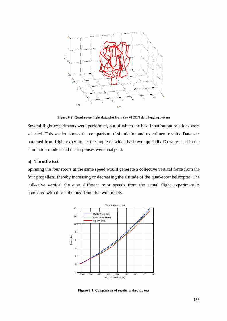
133
Figure 6-3: Quad-rotor flight data plot from the VICON data logging system
Several flight experiments were performed, out of which the best input/output relations were
selected. This section shows the comparison of simulation and experiment results. Data sets
obtained from flight experiments (a sample of which is shown appendix D) were used in the
simulation models and the responses were analysed.
a) Throttle test
Spinning the four rotors at the same speed would generate a collective vertical force from the
four propellers, thereby increasing or decreasing the altitude of the quad-rotor helicopter. The
collective vertical thrust at different rotor speeds from the actual flight experiment is
compared with those obtained from the two models.
Figure 6-4: Comparison of results in throttle test
230 240 250 260 270 280 290 300 310-2
0
2
4
6
8
10
12
14
Motor speed (rad/s)
Forc
e (N
)
Total vertical thrust
Matlab/SimulinkReal ExperiementSolidWorks

134
It is quite clear from the graph that the curves are very similar, despite the difference in the
magnitude of the forces as the rotor speeds increase. The Matlab/Simulink model produced
the highest values of the three curves, while that of the Solidworks was the lowest with the
real flight experiments finding a narrow space in between the two curves.
According to the curves in figure 6-4, the largest error of about 0.4N in the Matlab/Simulink
model is recorded at speed 286rad/s, while the smallest of 0.017N is observed at speed
227.5rad/s. In the case of the Solidworks model, the largest error of about 0.36N is recorded
at speed 306.3rad/s and the lowest of 0.032N is found at 240.3rad/s.
The effect of a force of 0.4N could be quite significant when it comes to the perfomance and
control of a vehicle of this nature, considering its very light weight and very high sensitivity
to rotor speed changes.
b) Roll and Pitch tests
Differential thrust between opposite rotors provides roll and pitch torques. The torques are
created with respect to the x or y axes, making the quad-rotor to tilt about that axis. However,
the total vertical thrust should be maintained as in hovering. The angles and forces produced
at different tilt angles are compared in figures 6-5 and 6-6 below.
Figure 6-5: Comparison of simulated and measured roll and pitch angles
At most times, it is assumed that because of the symmetric nature of the quad-rotor, the
behaviour of the vehicle with regards to roll and pitch angles would be the same. As observed
from the curves in figures 6-5, the results are not exactly the same. It is clear that the
0 0.5 1 1.5 2 2.5 3 3.5 4-8
-6
-4
-2
0
2
4
6
8
10
Time (s)
Ang
le (d
eg)
Simulated and Measured angles of roll and pitch
Pitch angle - SimulinkPitch angle - ExperimentRoll angle - SimulinkRoll angle - Experiment

135
symmetry of the quad-rotor helicopter only holds in ideal situations, which are very rare to
come by.
Figure 6-6: Comparison of simulated and measured forces in roll and pitch tests
The components of forces are compared here and seen to be very similar again, but with
differences in their magnitudes. It was also observed from figure 6-6 that there was a loss of
about 0.3N in the collective vertical thrust, which led to a loss in altitude in the
Matlab/Simulink model, signifying that the total vertical thrust was not maintained as
expected, because of the absence of a controller that would stabilise it when the thrust vector
is tilted as a result of the pitch angle.
c) Yaw test
Differential thrust between the two pairs of counter-rotating rotors provides the yaw torque.
The torque imbalance with respect to the z axis makes the quad-rotor turn about the same
axis. Normally, it is expected that the total vertical thrust is still maintained as in hovering.
Again very similar results are obtained for the yaw command, showing very comparable
angles and a near constant vertical thrust in figures 6-7 and 6-8 respectively.

136
Figure 6-7: Comparison of simulated and measured yaw angles
While the differences between the simulated and measured angles are not far apart, the
performance and control of the quad-rotor helicopter could still be hampered when it comes
to missions that require very high precision manouveres, especially when the vehicle
encounters a disturbance or an obstacle or even when a swarm of quad-rotors are working
together in close proximity.
Figure 6-8: Comparison of simulated and measured forces as a result of different yaw angles
While the total vertical thrusts in the two models increased gradually as the yaw angle
increased, that of the real flight experiment looked more stable. This goes on to emphsize the
need for a good controller for the models.
0 0.5 1 1.5 2 2.5 3 3.5 40
2
4
6
8
10
12
14
16
18
20
time (s)
Ang
le (d
eg)
Simulated and Measured angles of yaw
Yaw angle - ExperimentYaw angle - Simulink
0 2 4 6 8 10 12 14 16 18 200
0.1
0.2
0.3
0.4
0.5
0.6
0.7
0.8
0.9
1
Angle (deg)
Forc
e (N
)
Forces as a result of different yaw angles
Z-component of SimulinkZ-component of SolidWorksZ-component of Experiment

137
From the results obtained in the two models, the behaviour of the quad-rotor helicopter in
simulation resembles its behaviour in actual flight; thereby corroborating the fact that the two
models developed in chapters 3, 4 and 5 are good (though not perfect) representations of the
dynamics of the actual helicopter. However, the neural network error compensation promises
more reliable and accurate results.
6.2 Error Compensation using Artificial Neural Networks
Artificial neural networks are used in many important engineering and scientific applications,
some of which are signal enhancement, noise cancellation, pattern classification, system
identification, prediction, error compensation and control.
Neural networks provide a reliable tool for the fast solution of repetitive nonlinear curve
fitting problems. In fitting a curve, a neural network is trained using a set of inputs in order to
produce an associated set of target outputs. Once the neural network has fit the data, it forms
a generalization of the input-output relationship and can be used to generate outputs for
inputs it was not trained on [103].
The neural network design and training was done in the Matlab/Simulink environment and
data obtained from actual flight experiments were used for off-line training of the network.
Neural network training in the Matlab/Simulink environment is normally done using one of
the built-in functions incorporated in its Neural Network Toolbox.
The problem at hand is that of function approximation and the whole idea is to diminish the
error between the simulation results and the actual flight experiments to the barest minimum.
6.2.1 Compensation Architecture
The compensation system used here adopts a post correction technique. It takes its inputs from
the two models (Matlab/Simulink and Solidworks) developed in chapters 4 and 5 respectively
as shown in figure 6-9 below. The system, having been trained with data obtained from
actual flight experiments, computes the compensation value of the two simulation models.
The output of the system is the data used to train the quad-rotor fuzzy-neural controller.

138
Figure 6-9: Artificial neural network correction system
The neural network architecture is made up of layers of nodes (input, hidden and output)
which are the processing units. The input nodes receive directly the output data from the two
models, the hidden nodes process the data while the output node gives out the corrected
value. The output of the nodes is given by:
)(∑ +=i
iijj bowFs (6-1)
Where F is the activation function, io is the output from the thi node of the k-1 layer, ijw is
the weight and b the bias.
A simple neural network with two input neurons, 30 neurons in the hidden layer with a log-
sigmoid activation function, and a single output neuron was used for the compensation as
shown in figure 6-9. Computation of the compensation values was done by calculating the
feed-forward action of the network.
Table 6-1 shows a small sample of the errors before the neural network compensation was
done.
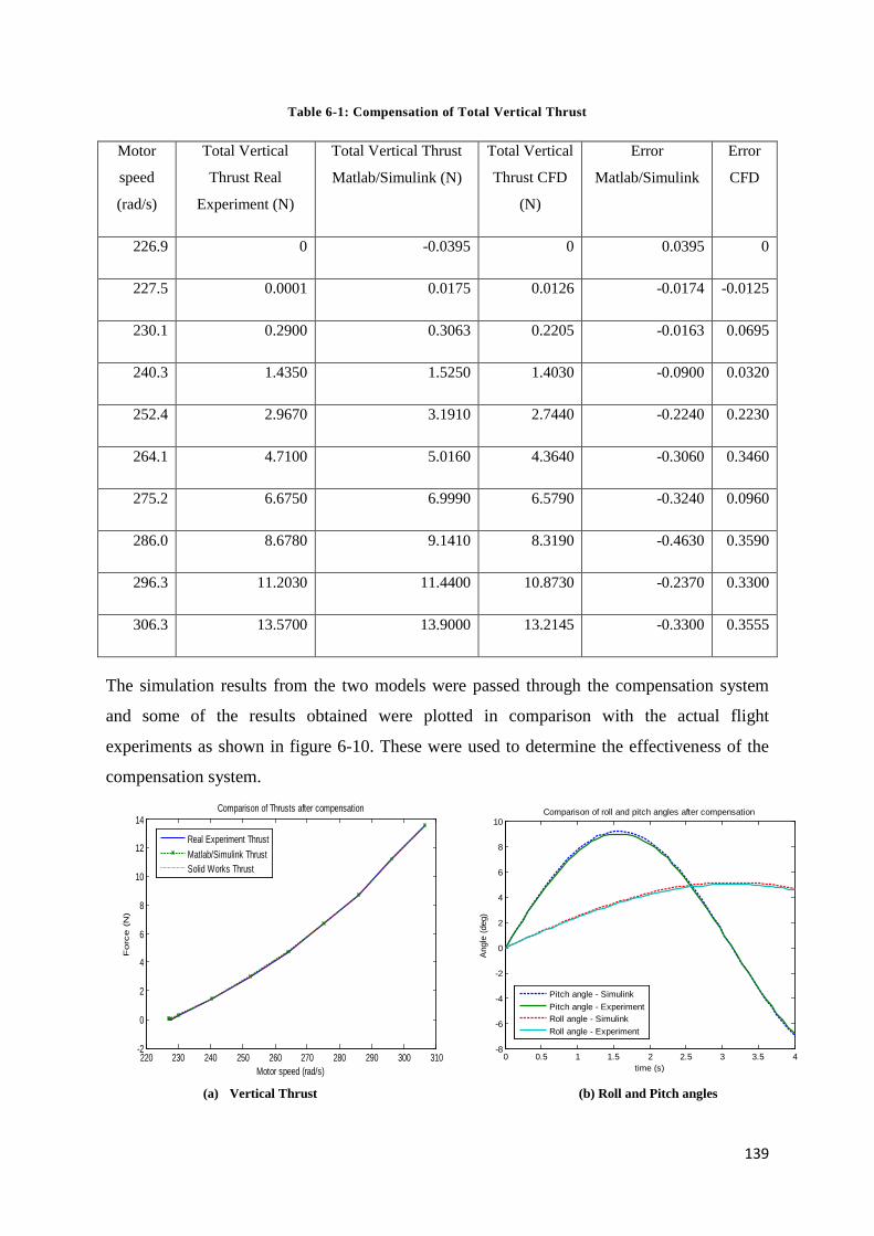
139
Table 6-1: Compensation of Total Vertical Thrust
Motor
speed
(rad/s)
Total Vertical
Thrust Real
Experiment (N)
Total Vertical Thrust
Matlab/Simulink (N)
Total Vertical
Thrust CFD
(N)
Error
Matlab/Simulink
Error
CFD
226.9 0 -0.0395 0 0.0395 0
227.5 0.0001 0.0175 0.0126 -0.0174 -0.0125
230.1 0.2900 0.3063 0.2205 -0.0163 0.0695
240.3 1.4350 1.5250 1.4030 -0.0900 0.0320
252.4 2.9670 3.1910 2.7440 -0.2240 0.2230
264.1 4.7100 5.0160 4.3640 -0.3060 0.3460
275.2 6.6750 6.9990 6.5790 -0.3240 0.0960
286.0 8.6780 9.1410 8.3190 -0.4630 0.3590
296.3 11.2030 11.4400 10.8730 -0.2370 0.3300
306.3 13.5700 13.9000 13.2145 -0.3300 0.3555
The simulation results from the two models were passed through the compensation system
and some of the results obtained were plotted in comparison with the actual flight
experiments as shown in figure 6-10. These were used to determine the effectiveness of the
compensation system.
(a) Vertical thrust (b) Roll and Pitch angles
220 230 240 250 260 270 280 290 300 310-2
0
2
4
6
8
10
12
14
Motor speed (rad/s)
Forc
e (
N)
Comparison of Thrusts after compensation
Real Experiment ThrustMatlab/Simulink ThrustSolid Works Thrust
(a) Vertical Thrust
0 0.5 1 1.5 2 2.5 3 3.5 4-8
-6
-4
-2
0
2
4
6
8
10
time (s)
Ang
le (d
eg)
Comparison of roll and pitch angles after compensation
Pitch angle - SimulinkPitch angle - ExperimentRoll angle - SimulinkRoll angle - Experiment
(b) Roll and Pitch angles

140
Figure 6-10: Results of Neural Network Compensation
Figure 6-10 shows that the neural network error compensation system was able to correct for
the modelling and simulation errors with all the curves almost super-imposing on one
another. The overall maximum average error was reduced from 0.11936 N to 0.01879 N –
15.74% of the uncompensated error.
6.3 Chapter Summary
Computations performed with an analytical model of the quad-rotor built in Matlab/Simulink
and those obtained using CFD (Computational Fluid Dynamics) on a 3-D Solidworks model
of the same helicopter have been compared with experiment data gathered from actual flight
experiments at Essex University. In [98], a general agreement between numerical and
experimental results was judged satisfactory and found to be good enough to validate the use
0 2 4 6 8 10 12 14 16 18 20-0.5
0
0.5
1
1.5
2
2.5
Angle (deg)
Forc
e (N
)
Comparison of pitch angle forces after compensation
X-component of ExperimentX-component of SimulinkX-component of SolidWorksZ-component of ExperimentZ-component of SimulinkZ-component SolidWorks
(c) Forces as a result of pitch angles
-20-18-16-14-12-10-8-6-4-20-0.5
0
0.5
1
1.5
2
2.5
Angle (deg)
Forc
e (
N)
Comparison of roll angle forces after compensation
Y-component of ExperimentY-component of SimulinkY-component of SolidWorksZ-component of ExperimentZ-component of SimulinkZ-component of SolidWorks
(d) Forces as a result of roll angles
0 0.5 1 1.5 2 2.5 3 3.5 40
2
4
6
8
10
12
14
16
18
20
time (s)
Ang
le (d
eg)
Comparison of yaw angles after compensation
Yaw Angle - ExperimentYaw Angle - Simulink
(e) Yaw angles
0 2 4 6 8 10 12 14 16 18 200
0.1
0.2
0.3
0.4
0.5
0.6
0.7
0.8
0.9
1
Angle (deg)
Forc
e (
N)
Comparison of yaw angle forces after compensation
Z-component of ExperimentZ-component of SimulinkZ-component of SolidWorks
(f) Forces as a result of yaw angles

141
of the CFD simulation results for future wind flow analysis and prediction of the helicopter
movements. It was also thought that more reliable and accurate simulation results would
improve the performance and control design of the quad-rotor helicopter, especially in the
rejection of and recovery from a disturbance [103]. This is because of the helicopter’s
inherent sensitivity to rotor speed changes and disturbances like wind gusts.The use of
function approximation in this chapter clearly shows that a neural network is a viable
technology for computing compensation values for the quad-rotor modelling and simulation
errors.

142
CHAPTER 7
INTELLIGENT CONTROLLER DESIGN
This chapter presents the development of a robust adaptive fuzzy-neural controller for quad-
rotor helicopters. Data obtained from simulations of the models developed in chapters 4, 5
and 6 of this thesis are used to train a fuzzy-neural system, made up of a hierarchy of
controllers to control the attitude and position of the quad-rotor helicopter.

143
7.0 Aircraft Navigation in the Wind
Aircrafts moving though still air generally move in the direction they are pointed. However
the wind will always alter the course and speed of the craft relative to the ground depending
on the wind direction and speed.
The relatively low weight and cruising speed of quad-rotor helicopters make them
susceptible, particularly in strong winds. Consequently the computation of the effect of wind
on aircraft movement relative to the ground is a major part of UAV flight planning and
navigation.
The problem is one of trigonometry; the vector triangle involving wind speed and direction,
air speed and heading, ground speed and track must be solved. Figure 7-1 illustrates the
problem. The triangle is geometrically laid out with the known quantities (e.g., wind speed
and direction forms one vector, the desired track determines the orientation of the second side
and the desired air speed forms the magnitude of the third) [95].
1. The wind vector represents the motion of the air mass over the ground. It is defined by
wind direction and wind speed.
2. The heading vector represents the motion of the aircraft through the air mass. It is defined
by heading angle and air speed.
3. The ground vector represents the motion of the aircraft over the ground. It is defined by
ground track and ground speed. The ground vector is the resultant of algebraically adding
the air vector and the wind vector.
Figure 7-1: Navigation vector relationship

144
In this case, the speeds or distances covered can be used, because they are directly
proportional. Under constant input conditions, a flight for any length of time would cover a
distance proportional to the speed of the helicopter; therefore the wind triangle would have
exactly the same shape, whichever variable is used.
The ends of the wind speed vector determine two points of the triangle; the intersection of an
arc, whose radius represents the air speed magnitude, with the straight line defining the
desired track is the third point. Thus the helicopter heading required to maintain track and
groundspeed along that track are determined.
𝑣𝑒 = 𝑢 + 𝑢𝑤 (7-1)
Where 𝑣𝑒 is the inertial velocity vector made up of the ground speed and track;𝑢 is air speed
vector made up of heading and air speed and 𝑢𝑤 is the wind vector made up of the wind
speed and direction.
The motion of the helicopter in turbulence is akin to that of a ship on a rough sea or an
automobile on a rough road. It is subjected to buffeting by random external forces, so that the
attitude angles and trajectory vary randomly with time. These changes cause corresponding
changes in forces and moments felt by the helicopter, resulting in structural forces and
moments and vehicle motions [104].
7.1 Neural Network Model
As stated in chapter 2, artificial neural networks are among the newest control technologies in
this day and age. The field of work is interdisciplinary, with lots of applications in everyday
life. Just like its biological predecessor, an artificial neural network is an adaptive system -
meaning that parameters change during its operations and are deployed to solve problems as
they develop.
Neural networks are developed using a logical step-by-step process, which optimizes a
criterion commonly known as the learning rule. The training data are important for these
networks, as they convey the information that is necessary for determining the optimal
operating point. Furthermore, the non-linear characteristics associated with neural networks
make them very flexible processing systems [80].
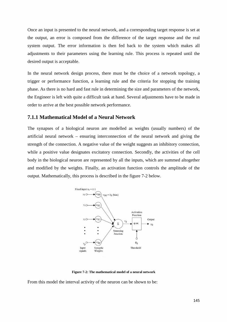
145
Once an input is presented to the neural network, and a corresponding target response is set at
the output, an error is composed from the difference of the target response and the real
system output. The error information is then fed back to the system which makes all
adjustments to their parameters using the learning rule. This process is repeated until the
desired output is acceptable.
In the neural network design process, there must be the choice of a network topology, a
trigger or performance function, a learning rule and the criteria for stopping the training
phase. As there is no hard and fast rule in determining the size and parameters of the network,
the Engineer is left with quite a difficult task at hand. Several adjustments have to be made in
order to arrive at the best possible network performance.
7.1.1 Mathematical Model of a Neural Network
The synapses of a biological neuron are modelled as weights (usually numbers) of the
artificial neural network – ensuring interconnection of the neural network and giving the
strength of the connection. A negative value of the weight suggests an inhibitory connection,
while a positive value designates excitatory connection. Secondly, the activities of the cell
body in the biological neuron are represented by all the inputs, which are summed altogether
and modified by the weights. Finally, an activation function controls the amplitude of the
output. Mathematically, this process is described in the figure 7-2 below.
Figure 7-2: The mathematical model of a neural network
From this model the interval activity of the neuron can be shown to be:

146
∑=
=p
jjkjk xwv
1
The output of the neuron ky , would therefore be the outcome of some activation function on
the value of kv .
7.1.2.1 Activation Functions
The activation function serves the purpose of a squashing function, such that the output of a
neuron is between specified values (typically 0 and 1, or -1 and 1) as shown in figure 7-3
below. In general, there are three types of activation functions.
First, there is the Threshold Function which takes on a value of 0 if the summed input is less
than a certain threshold value (v), and the value 1 if the summed input is greater than or equal
to the threshold value.
<≥
=0001
)(ifvifv
vϕ
Secondly, there is the Piecewise-Linear function. This function again can take on the values
of 0 or 1, but can also take on values between that depending on the amplification factor in a
certain region of linear operation.
−≤
>>−
≥
=
210
21
21
211
)(
v
vv
v
vϕ
Thirdly, there is the sigmoid function. This function can range between 0 and 1, but it is also
sometimes useful to use the -1 to 1 range. An example of the sigmoid function is the
hyperbolic tangent function.
)exp(1)exp(1)
2tanh()(
vvvv
−+−−
==ϕ

147
Figure 7-3: Neural Network activation functions
7.1.2.2 Neural Network Topology
The focus here is on the pattern of connections between the units and the propagation of data.
The main distinction that can be made is between:
Feed-forward neural networks, where the data flow from input to output units is
strictly feed-forward. The data processing can extend over multiple (layers of) units,
but no feedback connections are present. In other words, there are no connections
extending from outputs of units to inputs of units in the same layer or other layers.
Recurrent neural networks that do contain feedback connections. Contrary to feed-
forward networks, the dynamical properties of the network are important. In some
cases, the activation values of the units undergo a relaxation process such that the
neural network will evolve to a stable state in which these activations do not change
anymore. In other applications, the changes of the activation values of the output
neurons are significant, such that the dynamical behaviour constitutes the output of
the neural network [84].

148
7.1.2.3 Neural Network Training
A neural network has to be configured such that the application of a set of inputs produces
(either 'direct' or via a relaxation process) the desired set of outputs. There are numerous
methods of setting the strengths of the connections. One way is to set the weights explicitly,
using a priori knowledge. Another way is to train the neural network by feeding it teaching
patterns and letting it change its weights according to a specified learning rule.
Training and learning functions are mathematical procedures used to automatically adjust the
network's weights and biases as shown in figure 7-4 below. The training function dictates a
global algorithm that affects all the weights and biases of a given network. The learning
function can be applied to individual weights and biases within a network.
Figure 7-4: Neural Network training
Learning situations can be categorised into the following:
1. Supervised learning or Associative learning in which the network is trained by providing
it with input and matching output patterns. These input-output pairs can be provided by
an external teacher, or by the system which contains the neural network (self-supervised).
2. Unsupervised learning or Self-organisation in which an (output) unit is trained to respond
to clusters of pattern within the input. In this paradigm the system is supposed to discover
statistically salient features of the input population. Unlike the supervised learning
paradigm, there is no a priori set of categories into which the patterns are to be classified;
rather the system must develop its own representation of the input stimuli.
3. Reinforcement Learning. This type of learning may be considered as an intermediate
form of the above two types of learning. Here the learning machine does some action on
the environment and gets a feedback response from the environment. The learning system
grades its action good (rewarding) or bad (punishable) based on the environmental

149
response and accordingly adjusts its parameters. Generally, parameter adjustment is
continued until an equilibrium state occurs, following which there will be no more
changes in its parameters. The self-organizing neural learning may be categorized under
this type of learning.
7.2 Fuzzy Set Theory used in the Neural Network Model
The notion of fuzzy logic is very similar to human reasoning and inference process. Unlike
classical control strategy, which is point-to-point control, fuzzy logic control is a range-to-
point or range-to-range control. The output of a fuzzy controller is derived from
fuzzifications of both inputs and outputs using the associated membership functions. A crisp
input will be converted to the different members of the associated membership functions
based on its value. From this point of view, the output of a fuzzy logic controller is based on
its memberships of the different membership functions, which can be considered as a range
of inputs [105].
The idea is to map an input space to an output space, and the principal mechanism for doing
this is a list of if-then statements referred to as rules. All rules are evaluated in parallel, not
really minding the order in which they come. These rules refer to the variables and adjectives
that describe those variables. For a system that interprets rules as is the case with fuzzy logic,
it is very important to define the terms to be used and the adjectives that describe them right
from the beginning. Figure 7-5 shows a good description of a section of the fuzzy system.
Figure 7-5: Fuzzy inference system for quad-rotor control
150
Fuzzy inference interprets the values in the input vector and, based on some set of rules,
assigns values to the output vector.
Fuzzy logic begins with the theory of a fuzzy set. A fuzzy set is one without crisp, clearly
defined boundaries. It could be made up of components with only a partial degree of
membership.
Any statement can be fuzzy. The major advantage that fuzzy reasoning offers is the ability to
reply to a yes-no question with a not-quite-yes-or-no answer. Human beings do such things
many times a day, but it is a rather new ‘knowledge’ for computers and machines. Reasoning
in fuzzy logic is just a matter of generalizing the familiar true-false, on-off, yes-no (Boolean)
logic. If the numerical value of 1 is given to true and 0 given to false, fuzzy logic also permits
in-between values like 0.3, 0.675 and many more.
7.2.1 Membership Functions
A membership function (MF) is a curve that defines how each point in the input space is
mapped to a membership value (or degree of membership) between 0 and 1 as shown in
figure 7-6 below. The input space is sometimes referred to as the universe of discourse.
The only condition a membership function must really satisfy is that it must vary between 0
and 1. The function itself can be an arbitrary curve whose shape can be defined as any
suitable function from the point of view of simplicity, convenience, speed, and efficiency.
It is known that a classical set might be expressed as
A = x | x > 6
A fuzzy set is an extension of a classical set. If X is the universe of discourse and its elements
are denoted by x, then a fuzzy set A in X is defined as a set of ordered pairs.
A = x, µA(x) | x ∈ X
µA(x) is called the membership function (or MF) of x in A. The membership function maps
each element of X to a membership value between 0 and 1.
The basic membership functions are:
piece-wise linear functions

151
the Gaussian distribution function
the sigmoid curve
quadratic and cubic polynomial curves
Figure 7-6: Fuzzy logic membership functions [105]
The most important thing to realize about fuzzy logical reasoning is the fact that it is a
superset of the standard Boolean logic. In other words, if you keep the fuzzy values at their
extremes of 1 (completely true) or 0 (completely false), standard logical operations will hold.
7.2.2 If-Then Rules
Fuzzy sets and fuzzy operators are the subjects and verbs of fuzzy logic. The if-then rule
statements are used to formulate the conditional statements that comprise fuzzy logic. The
general form of a single fuzzy if-then rule is:
if x is A then y is B
Where A and B are linguistic values defined by fuzzy sets on the ranges X and Y,
respectively. The if-part of the rule "x is A" is called the antecedent or premise, while the
then-part of the rule "y is B" is called the consequent or conclusion.
The interpretation of an if-then rule involves the following:
1. Fuzzify inputs: Resolve all fuzzy statements in the antecedent to a degree of membership
between 0 and 1. If there is only one part to the antecedent, then this is the degree of
support for the rule.
2. Apply fuzzy operator to multiple part antecedents: If there are multiple parts to the
antecedent, apply fuzzy logic operators and resolve the antecedent to a single number
between 0 and 1. This is the degree of support for the rule.

152
3. Apply implication method: Use the degree of support for the entire rule to shape the output
fuzzy set. The consequent of a fuzzy rule assigns an entire fuzzy set to the output. This
fuzzy set is represented by a membership function that is chosen to indicate the qualities of
the consequent. If the antecedent is only partially true, (i.e., is assigned a value less than
1), then the output fuzzy set is truncated according to the implication method.
7.3 Fuzzy-Neural Model for the Quad-rotor Helicopter
Neural networks and fuzzy logic have shown great capabilities in solving many problems, but
have not yet been able to solve the really complex problems that their biological counterparts
can (e.g., vision). It is useful to fuse neural networks and fuzzy systems to offset the demerits
of one technique by the merits of another technique.
Hybrid fuzzy-neural systems are homogeneous and usually resemble neural networks. In this
case, the fuzzy system is construed as special kind of neural network. The advantage of such
a system is its architecture, which sees both systems fully fused as one entity and its ability to
learn online and offline as shown in figure 7-7.
Figure 7-7: Hybrid FNN Model for Quad-rotor Control
As shown in figure 7-7 above, the rule base of a fuzzy system is interpreted as a neural
network. The fuzzy sets can be regarded as weights whereas the input and output variables
and the rules are modelled as neurons. Neurons can be included or deleted in the learning
step. Finally, the neurons of the network represent the fuzzy knowledge base. Obviously, the

153
capabilities of both systems (as highlighted in section 2.5.1 of chapter 2 of this thesis) are
thus exhibited.
As stated in the previous section, membership functions that express the linguistic terms of
the inference rules must be defined in order to start building a fuzzy controller. The
optimization of these functions in terms of generalizing the data is very important to any
fuzzy systems, a solution which the neural networks can provide.
When the shapes of the membership functions are chosen, the neural network can then
optimize the parameters using the gradient descent algorithm. This implies that in addition to
providing details of the membership function shapes, there must be data to be used for
training – which was obtained from the models built in chapters 4 and 5 and validated in
chapter 6 of this thesis.
7.4 Controller design
Having established a satisfactory model of the quad-rotor system dynamics, based on the
validation with real flight experiment data, it is of great significance to show how a controller
is developed using fuzzy-neural networks as the chosen control technique. The structure in
figure 7-8, gives a description of the entire control system.
Flying a quad-rotor helicopter is a challenging task because of its inherent sensitivity to rotor
speed changes. It is even more difficult in the presence of a disturbance like wind. Data
obtained from the validated models in chapter 6 of this thesis have been used to train the
fuzzy-neural network system.
The controller implements these gained controls in the form of a command to the quad-rotor
system. The plant responds to the changes in the control variables, and then sensors detect
actual motion or state of the vehicle. The error between the desired input and the actual
measured input from the sensor is fed back into the controller where it adjusts the command
to attain the desired results as shown in figure 7-9.

154
Figu
re 7
-8: H
ybri
d FN
N C
ontr
ol S
yste
m fo
r Q
uad-
roto
r H
elic
opte
rs

155
A hierarchy of controllers was developed for the quad-rotor instead of having a single
controller, for more effective management of the states of the helicopter as shown in figure 7-
9 below. Training the initial single controller was quite a difficult task because of the nature
of data and the sensitivity of the quad-rotor helicopter to little changes in the speeds of it
motors.
Figure 7-9: Controller framework
At the top of the hierarchy is the position controller, which directs the movement of the quad-
rotor by providing the lower level controller (the attitude controller) with the desired roll,
pitch, and yaw angles in addition to the helicopter’s velocity. The attitude controller is
comprised of four lower level controllers that autonomously direct the rotor speed changes,
using voltage inputs to control the four attitude variables of throttle, roll, pitch and yaw as
shown in figure 7-10 below.
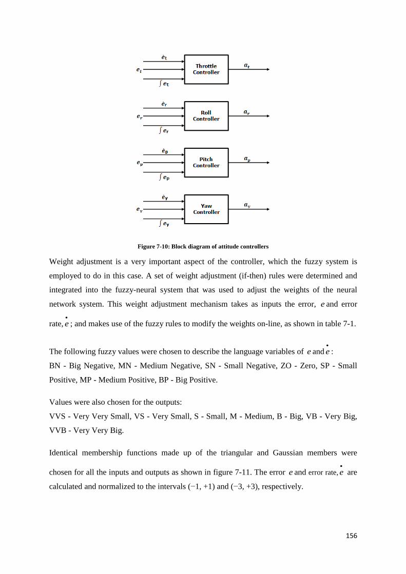
156
Figure 7-10: Block diagram of attitude controllers
Weight adjustment is a very important aspect of the controller, which the fuzzy system is
employed to do in this case. A set of weight adjustment (if-then) rules were determined and
integrated into the fuzzy-neural system that was used to adjust the weights of the neural
network system. This weight adjustment mechanism takes as inputs the error, e and error
rate,•
e ; and makes use of the fuzzy rules to modify the weights on-line, as shown in table 7-1.
The following fuzzy values were chosen to describe the language variables of e and•
e :
BN - Big Negative, MN - Medium Negative, SN - Small Negative, ZO - Zero, SP - Small
Positive, MP - Medium Positive, BP - Big Positive.
Values were also chosen for the outputs:
VVS - Very Very Small, VS - Very Small, S - Small, M - Medium, B - Big, VB - Very Big,
VVB - Very Very Big.
Identical membership functions made up of the triangular and Gaussian members were
chosen for all the inputs and outputs as shown in figure 7-11. The error e and error rate,•
e are
calculated and normalized to the intervals (−1, +1) and (−3, +3), respectively.

157
Figure 7-11: Membership functions for inputs and outputs
The rule base is also very important to any fuzzy system. As easy as it sometimes feels,
translating experience from an expert into such fuzzy rules; it gets more complicated and
confusing as the rules required to define the actions of the controller become too many [106].
Table 7-1: Fuzzy rule matrix for neural network weight adjustment
An example of the rules interpretation is given below:
From the second column and last row, if the error is BN (i.e. a Big Negative value) and the
error rate is BP (i.e. a Big Positive value) then the adjustment should be M (i.e. a Medium
value).
Since a dynamical system cannot understand such a value as a control input, there must be a
conversion, back to numbers that can serve as the control input – a process called
defuzzification, which practically the conclusion from the shared fuzzy weight as shown in
figure 7-7.

158
7.4.1 Attitude Controller
Flight in the desired direction and the general stabilization of the quad-rotor helicopter are
directed by this controller. Based on the commands from the position controller and
information received from sensors, it re-arranges the speeds of the rotors by changing the
voltage supply as described in figure 7-12. The action of this controller ensures that the
vehicle flies along the commanded path and at the desired speed.
Figure 7-12: Attitude controller framework
The position controller sends information about the desired attitude and the sensors provide
information about the current state of the quad-rotor helicopter in flight. A communication
with the ground station also gives the quad-rotor helicopter good information with regards to
the changing wind speeds when GPS signals are not available.
Collating all the information would give the controller a good understanding of what
adjustments are expected since the error between the desired and actual variables, together
with the derivatives and integrals of those errors are known. The controller now knows about
the absolute error and the rate of change of it, therefore it is able to compute the desired rotor
voltages for all four rotors, accordingly.
The four independent controllers that make up the attitude controller (equation 7-2) regulate
against any disturbance the upward velocity, together with the roll, pitch, and yaw angles
using the appropriate input combinations. These four attitude parameters use the following
combination:

159
−+=+−=−−=++=
ypt
yrt
ypt
yrt
aaaVaaaVaaaVaaaV
4
3
2
1
(7-2)
Where iV is the voltage input of each motor, ta , ra , pa and ya are the modifications made to
control the upward velocity, roll, pitch and yaw angles.
Data generated for throttle, roll, pitch and yaw were used in the training of each of the
controllers independently. This resulted in very quick learning of their separate actions on the
quad-rotor helicopter. After the training, the four simple controllers were arranged as shown
in figure 7-10. This gave rise to a single attitude controller that produces the desired rotor
speeds from the twelve inputs fed to the attitude controller as shown in figure 7-13.
Figure 7-13: The attitude controller voltage combination
7.4.1.1 Attitude Controller Training
Iterative training is conducted to minimize the mean square error (MSE) using the hybrid
optimization method (a combination of least squares and back propagation gradient descent
method). The reason for training is to obtain the most suitable and optimized values of the
weights for closest prediction through iterations. The training process is iterative and can be
stopped either when total training error reaches a bottom threshold or when training error
ceases to decrease any further. There is flexibility for varying number of neurons in the
160
hidden layers to optimize error. Starting from a small number of neurons, the number can be
gradually increased or decreased until an accepted training error is achieved [107].
Before training the fuzzy-neural system (off-line), the data set was divided into training, test
and validation sets. The training set was used to tune the fuzzy-neural model, while the test
set was used to determine when the training should be terminated, so as to prevent over-
fitting. The validation set was used to check the performance of the network.
A convenient start point of stable hover at a height of about 1m was chosen. A fuzzy-neural
controller was trained with data obtained for each of the Euler angles. During the training,
each of the controllers was given a set of data points that were expected to cover the range of
motion: 4
,4
ππ− for the roll and pitch controllers, since a little tilt would lead to acceleration
in the direction of tilt. The yaw controller had a range of ππ ,− , since the quad-rotor is able to
change heading without much effects on the stability of the vehicle.
Training was carried out with at least 8000 data samples generated from the neural network
compensation model developed in chapter 6 of this thesis. Since at some point the rotor
speeds would need to be increased and at other points they would need to be reduced,
depending on the desired attitude variable, a hyperbolic tangent was used as the activation
function to give activated nodes values between -1 and 1.
Although the angles can be controlled independently of each other, the thrust adjustment will
differ between the roll and pitch angles of the quad-rotor helicopter. Increasing the throttle
adjustment when all the tilt angles of the quad-rotor are zero, will only increase the upward
velocity; but when the craft is tilted at a certain angle, an adjustment of the same amount will
give a different result . The quad-rotor will move vertically as well as horizontally because of
the component of force as a result of the tilt angle.
Each time a neural network is trained, can result in a different solution due to different initial
weight and bias values and different divisions of data into training, validation, and test sets.
As a result, different neural networks trained on the same problem can give different outputs
for the same input. To ensure that a neural network of good accuracy has been found, the
controllers were retrained several times.

161
A number of different configurations of the controllers were evaluated to correct such a
situation, making use of a wide range of roll and pitch values to be used in the evaluations.
When all four controllers were trained, they were integrated into a single attitude controller as
described earlier. A more environment-specific training can be done for this controller to
ensure a good handling of any kind of disturbance. For this research, training was provided
for indoor and outdoor conditions (with wind speeds reaching 15m/s in any direction).
When each training round was completed, the network performance was checked to
determine if any changes needed to be made to the training process, the network architecture
or the data sets. Figure 7-14 below shows how well the neural networks performed.
Figure 7-14: Neural network performance after training
The learning curve gives an indication as to how well the problem was learnt by the neural
network. It plots the mean squared error achieved at the end of every epoch (an epoch is
defined as one pass through of all training data through the network). Typically the mean
squared error decreases rapidly in the beginning and flattens out at a low value. The lower the
mean squared error the better the neural network has learnt the training data. The iteration at
0 20 40 60 80 100 120 140 160 180 200
10-6
10-4
10-2
100
102
Roll Best Validation Performance is 1.2699e-06 at epoch 200
Mea
n Sq
uare
d Er
ror
(mse
)
200 Epochs
TrainValidationTestBest
0 20 40 60 80 100 120 140 160 180 20010
-9
10-8
10-7
10-6
Throttle Best Validation Performance is 7.0506e-09 at epoch 200
Mea
n Sq
uare
d Er
ror
(mse
)
200 Epochs
TrainValidationTestBest

162
which the validation performance reached a minimum was 200. For all the curves, the
validation and test curves are very similar, suggesting a good result without over fitting.
The fuzzy-neural system provides as outputs a set of control inputs related to the operation
tasks to be performed in adjusting the speeds of each of the four motors accordingly. Each
node applies these control inputs to manage the speeds of the motors of the quad-rotor
helicopter. Figure 7-15 shows the surface comparison between the input values of the fuzzy-
neural system.
Figure 7-15: Surface comparison between the input values of the fuzzy-neural system
7.4.2 Position Controller
Attitude targets are required by the attitude controller in order to move the quad-rotor
helicopter from one point to another. These targets are provided by the position controller.
The position controller in this report is saddled with the task of directing the motion of the
quad-rotor helicopter from one point to another, given the x, y and z coordinates as shown in
figure 7-16.
Figure 7-16: The Position controller

163
The position controller receives as inputs the difference between the desired and present
positions in the x, y, and z directions; and also the velocity in three axes. The controller then
directs the quad-rotor by sending commands about the attitude needed to move towards the
desired position. Owing to the quad-rotor helicopter's tractability, only two attitude angles are
required to reach any given position. Unless there is a need for a change of heading during
certain missions to position the payload (e.g. camera) at a particular point, the yaw angle
could always be set to 0. This allows the full motion of the quad-rotor helicopter to be
controlled by only the roll and pitch angles in combination with the desired vertical velocity.
7.4.2.1 Position Controller Training
Training consisted of evaluating each potential controller based on the ability to reach a
desired position as well as the total distance travelled in doing so. The training data set
included a network of points covering every direction of motion from the origin. Very similar
training parameters were used as in the case of the attitude controller.
7.6 Chapter Summary
This chapter detailed the development of a fuzzy-neural controller for the quad-rotor
helicopter. Data obtained from the two models, which were passed through the neural
network error compensation system were used to train and simulate the fuzzy-neural network
behaviour in the Matlab/Simulink software environment.
Training was carried out with at least 8000 data samples for each controller. The learning
curves in figures 7-14 and 7-15 show how well the problem was learnt by the fuzzy-neural
network, with the mean squared error decreasing rapidly in the beginning and flattening out
at a very low value suggesting good results without any over fitting.

164
CHAPTER 8
SIMULATION RESULTS AND DISCUSSION
This chapter provides details of the simulation of the fuzzy-neural quad-rotor flight controller
developed in chapter 7 of this thesis. This is intended to demonstrate the success of the
developed controller in adapting to changing flight conditions. Results of the simulations are
displayed and the performance of the controller is analysed for no wind and windy situations,
where the quad-rotor experienced winds of different magnitudes.

165
8.0 Flight Controller Simulation
UAV control systems usually involve huge and complex tasks, making the design and testing
of such systems time consuming and very expensive. Chapter 7 discussed the controller
design for the quad-rotor helicopter, where the fuzzy-neural controller computes the control
inputs for any given situation. It is theoretically possible to fly the vehicle in an open loop by
sending these reference control signals to the quad-rotor helicopter. However, this will be
difficult to achieve in real flight situations because when the vehicle encounters wind
disturbances, noise and probably some model uncertainties, there will most certainly be speed
and flight path tracking errors. Besides, the quad-rotor helicopter needs a feedback of its
current states so as to ensure good stability and control [1].
In order to test the effectiveness of the developed fuzzy-neural controller, seven simulation
situations have been clearly defined. In all situations, the quad-rotor starts at hover at (0, 0, 1)
and consist of a short flight within less than 25 seconds to a point (66.15, 0, 1) about 66
metres north of the start point. The quad-rotor helicopter was commanded to keep up with
different speeds at a time it was also allowed to experience winds speeds of different
magnitudes that were either reducing or increasing its speed or pushing it off the flight path.
The controller’s task in simulation is to compensate the error in the roll and pitch angles, so
as to stabilize the quad-rotor helicopter at an altitude of 1m and to ensure that it keeps to the
desired speed and planned path. For the purpose of this simulation studies, the quad-rotor
commanded yaw angle was kept at 0, since it was expected to fly northwards without any
change of heading.
In consideration of the fact that during real flight situations, the quad-rotor helicopter
experiences a little bit of delays and possible saturation of the actuators’, owing to the
wireless communications and the dynamics of the actuators; discrete-step delay blocks were
built into the feedback loop and actuators models in Matlab/Simulink. Also, with the motors
having a maximum angular velocity of 380 rad/sec, another saturation block was placed
between the fuzzy-neural controller and the delay block to keep within the limits.

166
8.1 Flight Simulation in No Wind Situation
In this situation, flows around the rotor blades of the helicopter are somewhat steady and the
rotors assumed to be working under the same conditions, because the wind speeds in the three
directions (x, y and z) were kept at 0m/s.
The first stage of this simulation shows the quad-rotor helicopter in vertical flight, climbing
to a height of 1m as shown in figure 8-1. The quad-rotor is then required to fly to (66.15, 0,
1), a position about 66m north of the start point (0, 0, 1) within 20 seconds. The desired flight
path can be seen to be exactly the same with the commanded flight path, showing no errors
within the x, y and z positions as there is no disturbance in the flight conditions.
Figure 8-1: Quad-rotor flight simulation in a no wind situation
The vehicle follows the planned path, reaching the desired speed of 3.5m/s in 2 seconds. The
controller is able to keep the helicopter flying at the commanded speed and path without any
deviation. As can be seen in the graphs (figure 8-2), the velocity, pitch angle and height
remain constant throughout the flight, after reaching their peaks.
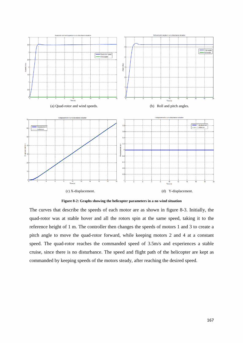
167
(a) Quad-rotor and wind speeds. (b) Roll and pitch angles.
(c) X-displacement. (d) Y-displacement.
Figure 8-2: Graphs showing the helicopter parameters in a no wind situation
The curves that describe the speeds of each motor are as shown in figure 8-3. Initially, the
quad-rotor was at stable hover and all the rotors spin at the same speed, taking it to the
reference height of 1 m. The controller then changes the speeds of motors 1 and 3 to create a
pitch angle to move the quad-rotor forward, while keeping motors 2 and 4 at a constant
speed. The quad-rotor reaches the commanded speed of 3.5m/s and experiences a stable
cruise, since there is no disturbance. The speed and flight path of the helicopter are kept as
commanded by keeping speeds of the motors steady, after reaching the desired speed.

168
Figure 8-3: Graph showing the speeds of the four motors of the quad-rotor in a no wind situation
As explained in Chapter 4 of this thesis, creating a forward pitch effect, entails increasing the
thrust in motor 3 (rear) and decreasing that of motor 1 (front), while keeping the other two
unchanged. To avoid yawing, the overall reaction torque must be equal to zero during flight.
This seems to impose a constraint on the amount of thrust that can be increased in one rotor
relative to the other. Since the thrust and the torque are quadratic with the motor speed, this
constraint does not mean that the speeds of the motor 1 and motor 3 are increased or
decreased by exactly the same amount, as clearly seen in the motor 1 and motor 3 curves in
figure 8-3.
In any case, maintaining a perfect balance of torques while the thrusts are being
independently modified is almost impossible, because the torques also depend on other
variables apart from the motor speed, such as the tangential velocities of the centres of the
rotors or the pitch rate. It is clearly seen that the controller increases the thrust in motor 3
more than it decreases that of motor 1, so as to maintain the altitude that would have been lost
to the thrust vector tilt as the quad-rotor pitches.
8.2. Flight Simulation in a Headwind
The horizontal wind velocity normally has a crosswind component and a headwind/tailwind
component, which affect its speed relative to the ground. When the quad-rotor helicopter
experiences such a flow of wind around it, there certainly will be unwanted moments in
addition to other possible effects that act due to the fact that the flight conditions are much
more unstable. The quad-rotor helicopter is likely to depart from equilibrium in flight,
leading to a possible loss of control.

169
The headwind component of the horizontal wind velocity would normally reduce the speed of
the quad-rotor, relative to the ground. By reducing the speed of the vehicle, the time required
to reach its destination is increased. Stronger winds could even prevent the vehicle from
reaching its destination, if there is no robust controller to help the vehicle recover from the
effects of the disturbance. In this study, two headwind situations are considered – constant
and gusty headwind situations.
8.2.1 Constant Headwind
This study describes a situation where a constant wind opposes the flight of the quad-rotor.
After reaching a height of 1m (0, 0, 1) as shown in figure 8-4, the quad-rotor is then required
to fly to the same position (66.15, 0, 1) from the start point within 20 seconds, similar to
study 1 above. The desired flight path is maintained, but with the opposing wind flow at
1.5m/s, the controller quickly re-arranges the speeds of the motors to counter the effect of the
wind and keep the helicopter in the desired speed.
Figure 8-4: Quad-rotor flight simulation in a headwind
In a constant headwind situation, the effects of the wind slamming the front of the quad-rotor
helicopter are seen from the graphs in figure 8-5. After reaching the desired speed of 3.5m/s
in 2 seconds and flying steadily for another 2 seconds, a constant headwind of speed 1.5m/s
was introduced to oppose the forward flight of the helicopter. The curves clearly show an
initial decline in the speed of the quad-rotor to 2.09m/s. The combined effect of the headwind

170
and the helicopter’s speed and forces always produces a resultant speed or force that is lower
than the one the helicopter had before it encountered the wind, though the thrust is increased
resulting in a little increase in altitude, which the controller nullifies almost immediately.
Stronger winds are expected to have a greater reduction effect on the quad-rotor’s speed and
forces.
The curves show oscillations in the quad-rotor velocity and pitch angle between 4 and 6
seconds of flight (exactly where the wind disturbance was introduced after the quad-rotor
reaches a steady cruise speed of 3.5m/s). It is clearly visible that the pitch angle is reduced,
while the resultant speed is lower than the commanded speed of the helicopter, with a
position error of 0.01m observed in the y-direction (east) from the plot. However, the action
of the controller immediately restores the speed of the helicopter to the commanded value of
3.5m/s and eliminates the y-position error, ensuring flight stability on the planned path
despite the 1.5m/s headwind effect.
(a) Quad-rotor and wind speeds. (b) Roll and pitch angles.
(c) X-displacement. (d) Y-displacement.
Figure 8-5: Graphs showing the helicopter parameters in a constant headwind
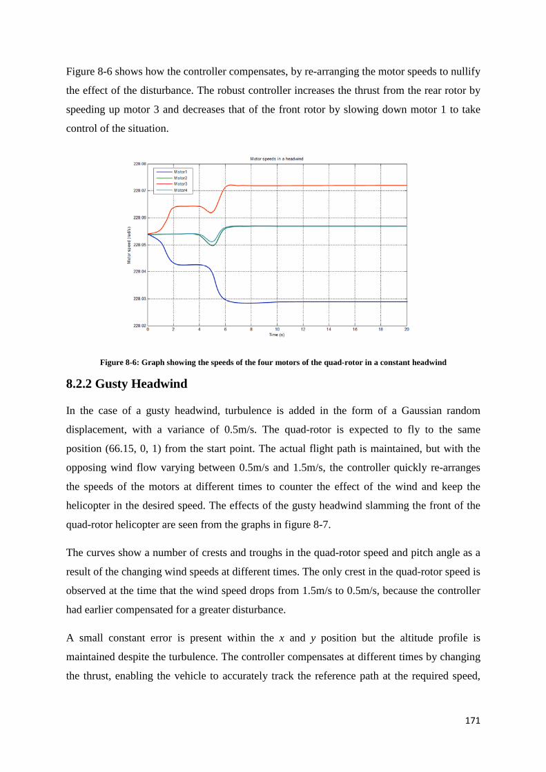
171
Figure 8-6 shows how the controller compensates, by re-arranging the motor speeds to nullify
the effect of the disturbance. The robust controller increases the thrust from the rear rotor by
speeding up motor 3 and decreases that of the front rotor by slowing down motor 1 to take
control of the situation.
Figure 8-6: Graph showing the speeds of the four motors of the quad-rotor in a constant headwind
8.2.2 Gusty Headwind
In the case of a gusty headwind, turbulence is added in the form of a Gaussian random
displacement, with a variance of 0.5m/s. The quad-rotor is expected to fly to the same
position (66.15, 0, 1) from the start point. The actual flight path is maintained, but with the
opposing wind flow varying between 0.5m/s and 1.5m/s, the controller quickly re-arranges
the speeds of the motors at different times to counter the effect of the wind and keep the
helicopter in the desired speed. The effects of the gusty headwind slamming the front of the
quad-rotor helicopter are seen from the graphs in figure 8-7.
The curves show a number of crests and troughs in the quad-rotor speed and pitch angle as a
result of the changing wind speeds at different times. The only crest in the quad-rotor speed is
observed at the time that the wind speed drops from 1.5m/s to 0.5m/s, because the controller
had earlier compensated for a greater disturbance.
A small constant error is present within the x and y position but the altitude profile is
maintained despite the turbulence. The controller compensates at different times by changing
the thrust, enabling the vehicle to accurately track the reference path at the required speed,

172
though it would take about 0.5 seconds more to arrive at the destination because of the
disturbance in the flight path.
(a) Quad-rotor and wind speeds. (b) Roll and pitch angles.
(c) X-displacement. (d) Y-displacement.
Figure 8-7: Graphs showing the helicopter parameters in a gusty headwind
Figure 8-8 shows how the controller compensates, by re-arranging the motor speeds to quash
the effect of the disturbance. The curves for motors 1 and 3 are seen to be changing within
very short intervals in response to the changing wind speed, which opposes the flight of the
vehicle. The arrangement of the motor speeds is seen to be carefully done so as to keep the
thrust and torque imbalance to the barest minimum in order to maintain the altitude and keep
the commanded zero yaw angle.

173
Figure 8-8: Graph showing the speeds of the four motors of the quad-rotor in a gusty headwind
8.3 Flight Simulation in a Tailwind
The tailwind component of the horizontal wind velocity would normally increase the speed of
the quad-rotor, relative to the ground. By increasing the speed of the vehicle, the time
required to reach its destination is reduced, which may be an advantage or disadvantage to the
vehicle, depending on the mission to be accomplished. With very strong winds, the vehicle
could go beyond the destination and have difficulty in returning if there is no robust
controller to help the vehicle recover from the effects of the disturbance. In this study, two
tailwind situations are considered – constant and gusty tailwind situations.
8.3.1 Constant Tailwind
This simulation study describes a situation where a constant wind hits the quad-rotor from the
rear, increasing its speed and possibly making it deviate from the planned path. Having
reached a height of 1m (0, 0, 1) as shown in figure 8-9, the quad-rotor is then commanded to
fly northwards to the same position (66.15, 0, 1) from the start point. The desired flight path
is maintained, but with the tailwind of 1.5m/s, the controller again has to re-adjust the motor
speeds in order to reduce the resultant speed of the helicopter to the desired speed and also
ensure that it keeps to the planned path.

174
Figure 8-9: Quad-rotor flight simulation in a tailwind
As the vehicle has an induced speed due to the tail wind there is need to reduce the pitch
angle, so as to slow it down and keep it on course. The graphs in figure 8-10 show
oscillations in the quad-rotor speed and pitch angle after 4 seconds of flight (exactly where
the wind disturbance was introduced, when the helicopter had reached a steady state).
Evidently, the speed of the quad-rotor is increased to a resultant velocity of about 5m/s. It is
also clear that the pitch angle of the helicopter is increased, but the swift action of the
controller reduces the pitch angle and restores the speed to the commanded value of 3.5m/s,
ensuring flight stability despite the tailwind effect.
(a) Quad-rotor and wind speeds. (b) Roll and pitch angles.

175
(c) X-displacement. (d) Y-displacement.
Figure 8-10: Graph showing the helicopter parameters in a constant tailwind
In compensating for the changes as a result of the tailwind, the controller re-arranges the
motor speeds to counter the effect of the wind and get it back to the commanded speed of
3.5m/s. Figure 8-11 shows the motor speed curves. The robust controller decreases the thrust
from the rear rotor by slowing down motor 3 and increases that of the front rotor by speeding
up motor 1 to take control of the situation.
Figure 8-11: Graph showing the speeds of the four motors of the quad-rotor in a constant tailwind
8.3.2 Gusty Tailwind
Just like in the case of a gusty headwind, the gusty tailwind also has turbulence added in the
form of a Gaussian random displacement, with a variance of 0.5m/s. The quad-rotor is
expected to fly to the same position (66.15, 0, 1) from the start point. The wind flow varying
between 0.5m/s and 1.5m/s in the direction of flight of the helicopter requires that the

176
controller quickly re-arranges the speeds of the motors at different times to reduce the quad-
rotor’s resultant speed to the desired speed. The effects of the gusty tailwind on the quad-
rotor helicopter are seen from the graphs in figure 8-12.
Again the curves show a number of crests and troughs in the quad-rotor velocity and pitch
angle owing to the changing wind speeds at different times. The controller compensates at
different times by changing the thrust, enabling the vehicle to accurately track the reference
path at the required speed, though it took about 0.6 seconds less to arrive at the destination
because of the push of the gusty tailwind.
(a) Quad-rotor and wind speeds. (b) Roll and pitch angles.
(c) X-displacement. (d) Y-displacement.
Figure 8-12: Graph showing the helicopter parameters in a gusty tailwind
Figure 8-13 shows how the controller compensates, by re-arranging the motor speeds to
quash the effect of the disturbance. The curves for motors 1 and 3 are seen to be changing
within very short intervals in response to the changing wind speed, which adds to the speed
of the helicopter. The arrangement of the motor speeds is seen to be carefully done so as to

177
keep the thrust and torque imbalance to the barest minimum in order to maintain the altitude
and keep the commanded zero yaw angle.
Figure 8-13: Graph showing the speeds of the four motors of the quad-rotor in a gusty tailwind
8.4 Flight Simulation in a Crosswind
A crosswind would normally create an in-plane force that acts on the vehicle and tends to
create a moment that makes the quad-rotor helicopter tilt. The instant the quad-rotor starts to
tilt, it accelerates in its direction of tilt. However, too much of a tilt would make the quad-
rotor to start loosing equilibrium, thereby leading to a possible oscillation and loss of control
of the whole vehicle. Only a timely and accurate re-arrangement of the motor speeds can
maintain that equilibrium, keeping the quad-rotor in the planned path and desired speed.
8.4.1 Constant Crosswind
This simulation study describes a situation where the wind hits the quad-rotor from the side,
giving it a resultant speed and trying to make it deviate from the planned path. The quad-rotor
is again required to fly northwards to the same position (66.15, 0, 1) from the start point. The
desired flight path is maintained from the start of the flight until a crosswind of 1.5m/s
blowing towards the east is encountered. This causes a little deviation of about 0.2m to the
east, before the controller is able to compensate and return the quad-rotor to the planned path
and desired speed.

178
Figure 8-14: Quad-rotor flight simulation in a crosswind
As shown in graphs in figure 8-15, the wind blows from the side of the helicopter causing a
disturbance, just after 4 seconds of flight. This disturbance creates a very small roll angle,
tending to upset the helicopter. A resultant speed, slightly higher than the commanded speed
of 3.5m/s is reached, with the pitch angle reduced and a little change in the height. The action
of the controller ensures a negative roll angle and a restoration of the speed of the helicopter
as commanded at the start of the flight.
(a) Quad-rotor and wind speeds. (b) Roll and pitch angles.

179
(c) X-displacement. (d) Y-displacement.
Figure 8-15: Graph showing the helicopter parameters in a constant crosswind
The motor speed curves in figure 8-16 show the reaction of the controller when the
disturbance is encountered. A constant crosswind of speed 1.5m/s in introduced after about 2
seconds of flight, blowing eastwards from the side of the helicopter to try to make it veer off
course. As a result of this disturbance, the velocity of the quad-rotor is increased to a
resultant velocity of 3.65 m/s in the NE direction as against the commanded speed of 3.5m/s.
The change of direction from north to north-east indicates a displacement in the y-direction
(east), owing to a roll angle created as a result of the disturbance. The robust controller slows
down and speeds up the motors accordingly to take control of the situation. It is observed in
figure 8-15 above [(c) and (d)] that the roll angle and y-displacement are reduced to a
negative and zero respectively to counter the effect of the crosswind. This restores the
helicopter to the commanded speed of 3.5m/s.
Figure 8-16: Graph showing the speeds of the four motors of the quad-rotor in a constant crosswind
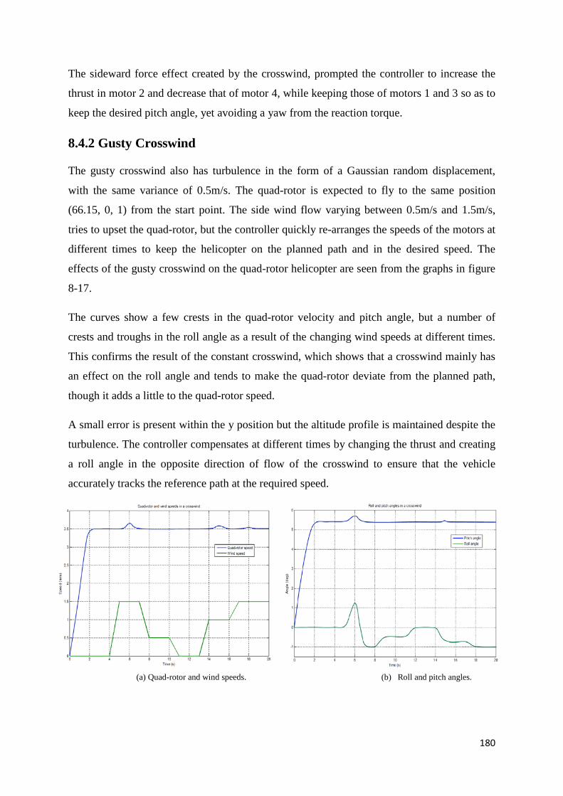
180
The sideward force effect created by the crosswind, prompted the controller to increase the
thrust in motor 2 and decrease that of motor 4, while keeping those of motors 1 and 3 so as to
keep the desired pitch angle, yet avoiding a yaw from the reaction torque.
8.4.2 Gusty Crosswind
The gusty crosswind also has turbulence in the form of a Gaussian random displacement,
with the same variance of 0.5m/s. The quad-rotor is expected to fly to the same position
(66.15, 0, 1) from the start point. The side wind flow varying between 0.5m/s and 1.5m/s,
tries to upset the quad-rotor, but the controller quickly re-arranges the speeds of the motors at
different times to keep the helicopter on the planned path and in the desired speed. The
effects of the gusty crosswind on the quad-rotor helicopter are seen from the graphs in figure
8-17.
The curves show a few crests in the quad-rotor velocity and pitch angle, but a number of
crests and troughs in the roll angle as a result of the changing wind speeds at different times.
This confirms the result of the constant crosswind, which shows that a crosswind mainly has
an effect on the roll angle and tends to make the quad-rotor deviate from the planned path,
though it adds a little to the quad-rotor speed.
A small error is present within the y position but the altitude profile is maintained despite the
turbulence. The controller compensates at different times by changing the thrust and creating
a roll angle in the opposite direction of flow of the crosswind to ensure that the vehicle
accurately tracks the reference path at the required speed.
(a) Quad-rotor and wind speeds. (b) Roll and pitch angles.

181
(c) X-displacement. (d) Y-displacement.
Figure 8-17: Graph showing the helicopter parameters in a gusty crosswind
The motor speed curves in figure 8-18 show the complexity of the controller action at the
different points that the disturbances are encountered. The speeds of the two sets of motors
are seen to be changed at different intervals to nullify the effect of the disturbance. As a result
of the disturbance, the speed of the quad-rotor was increased and reduced at different times
by either the disturbance or the action of the controller.
Figure 8-18: Graph showing the speeds of the four motors of the quad-rotor in a gusty crosswind

182
8.5 Discussion of Results
To demonstrate the robustness and effectiveness of the developed fuzzy-neural controller, a
number of different situations have been considered in this chapter. At the outset, steady
winds were applied along the x axis from the front (headwind) and from the rear (tailwind);
then another steady wind was applied along the y-axis from the side (crosswind). All
disturbances at this stage were kept at a constant speed of 1.5m/s.
Gusts with variance of 0.5m/s and a maximum of 1.5m/s were introduced in the simulation
system in the same directions as the steady winds to test the ability of the controller to control
the multi-variable flying states of the quad-rotor helicopter in complex weather conditions.
The graphs in figures 8-7, 8-12 and 8-17 showing the crests and troughs at different points of
increase (and decrease) of the wind speed, describe the motion of the vehicle as momentarily
departing from the reference trajectory with very small tracking errors.
For all the simulation studies, the commanded flight paths and target destinations have a
tolerance of 0.25m. The quad-rotor helicopter flight speed changed at different times in flight,
owing to the disturbances, but the vehicle still attempted to keep up with the commanded
speed and follow the planned path.
With a constant headwind opposing the flight of the vehicle, the controller had to create a
larger pitch angle to keep up with the commanded speed as shown in figure 8-5 (a) and (b). A
constant tailwind on the other hand created an induced velocity for the vehicle, hence the
controller reduced the pitch angle to slow it down and keep it going at the required speed as
shown in figure 8-10 (a) and (b). As can be seen in figures 8-7 (a) and (b) and 8-12 (a) and
(b), the effects of varying speeds of the headwind and tailwind made the control problem
more complex.
The lateral wind speed has a great influence on the thrust generated by the propellers, because
of the aerodynamic effects. In situations where the wind speed becomes too high, the quad-
rotor helicopter will find it very difficult to maintain the total vertical thrust and so the
altitude control becomes difficult too. Having carried out a number of simulations, it was
concluded that that the speed of the quad-rotor must not exceed 18 m/s and so a saturation
block was placed on the quad-rotor speed demand to keep it in check.
This limit was set because the quad-rotor helicopter must not pitch or roll too much otherwise
it would be vertically unstable. Therefore, the pitch and roll limits were set at θ ≤ ±28

183
degrees and φ ≤ ±28 degrees, because the speed of the quad-rotor helicopter is a function of
the tilt angles of pitch and roll respectively. Consequently, saturation blocks were also placed
on the pitch and roll angle demands to maintain the altitude and ensure more stability in
flight. This effect is also confirmed in the works of [54, 57] and also demonstrated in the
figures in appendix E.
The major effect of the crosswind is to deflect the flight path in the direction of the wind by
adding another vector component to the ground speed, with the aerodynamic lift force
depending on the speed of the wind. The controller had to roll the quad-rotor in opposition to
the wind as shown in figure 8-15 (a) and (b), so as to maintain its course. These simulation
studies highlight the advantage of Fuzzy-Neural Networks over a linear tracking controller in
following a reference speed and flight path, as it accounts for environmental changes such as
the presence of a disturbance such as wind.
Generally, when flying forward the quad-rotor is expected to maintain a negative pitch angle,
creating a horizontal component of the total thrust to overcome the drag of the airframe and
the in-plane forces over the rotors. The problem of loss of altitude is always encountered
when the quad-rotor starts a horizontal movement from hover and it even gets worse when
there are strong winds. The total vertical thrust is supposed to be maintained, thereby keeping
the helicopter at a constant height, but because of the thrust vector, this becomes difficult to
achieve. However, the fuzzy-neural controller has been able to keep the altitude steady by
increasing the total thrust when necessary and ensuring that if there is any loss, it is reduced
to the barest minimum.
The simulation results have shown the ability of the controller to reject disturbances - as seen
from the very small position and tracking errors. In situations where the disturbance is not
rejected, the quad-rotor helicopter is seen to quickly return to the reference path as a result of
the recovery action of the controller. The controller in re-arranging the speeds of the motors
was able to compensate, enabling the quad-rotor to reach its destination – though at some
times taking about 0.5 seconds longer than the required time.
8.6 Towards Implementation
The focus in this section is on the practical implementation of the control system that has
been developed during the research. The test-bed for the experiments would normally consist
of a complete quad-rotor helicopter, a ground station with computer, a radio base-station and
remote control as shown in figure 8–19.

184
The control algorithms are implemented on the ground station computer and run directly in
the Matlab/Simulink software environment. A special S-function block allows the Simulink
model to receive sensor data from the quad-rotor and to send back the motor input
commands. The block communicates via USB with the computer module in the ground
station. The sample rate is limited at 50 Hz by the speed of the wireless data link. All radio
communication is done in short packets with minimum latency in such a way that during the
sample period of 20 ms the sensors are sampled on the quad-rotor, the data is sent over radio
to the ground station and then through USB to the Simulink model, the results of the control
algorithm are in turn sent back through radio to the quad-rotor to control the electric motors.
The remote control uses the same two-way communication link to send commands to either
the quad-rotor or the computer (i.e. for reference inputs) and can also display important
process variables to the pilot on the ground.
Figure 8-19: Flight experiment control system
For such small vehicles flying outdoors, the real-world task of closing the loop by providing
feedback is always challenging. Larger UAVs have Inertial Navigational and Guidance
Systems that provide accurate rate and acceleration information as well as a GPS for
positional information. However, GPS is usually only accurate to a few meters which may
not be adequate for a small UAV such as the quad-rotor helicopter.
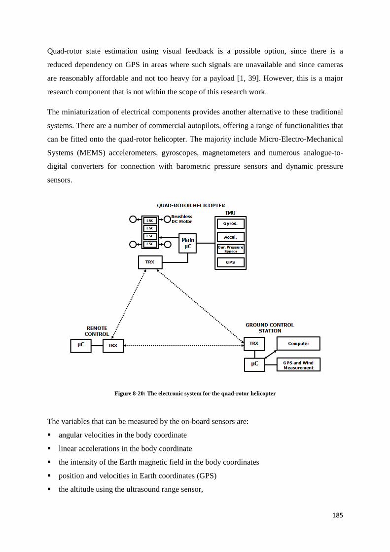
185
Quad-rotor state estimation using visual feedback is a possible option, since there is a
reduced dependency on GPS in areas where such signals are unavailable and since cameras
are reasonably affordable and not too heavy for a payload [1, 39]. However, this is a major
research component that is not within the scope of this research work.
The miniaturization of electrical components provides another alternative to these traditional
systems. There are a number of commercial autopilots, offering a range of functionalities that
can be fitted onto the quad-rotor helicopter. The majority include Micro-Electro-Mechanical
Systems (MEMS) accelerometers, gyroscopes, magnetometers and numerous analogue-to-
digital converters for connection with barometric pressure sensors and dynamic pressure
sensors.
Figure 8-20: The electronic system for the quad-rotor helicopter
The variables that can be measured by the on-board sensors are:
angular velocities in the body coordinate
linear accelerations in the body coordinate
the intensity of the Earth magnetic field in the body coordinates
position and velocities in Earth coordinates (GPS)
the altitude using the ultrasound range sensor,

186
temperatures of the gyroscopes, accelerometers and magnetic field sensors for calibration,
battery voltage and current,
motor rotation speeds.
On-board computation of the control action is reduces time lags, however, in an experimental
set up, the requirements could be different. The control law may need modification in flight
or at least a quick turn-around in between flights. Furthermore, the control algorithms
presented in this thesis are computationally demanding and therefore, while on-board
implementation is the eventual aim, off-board computation is the initial preferred option.
However, this in turn presents communication challenges with lag time being the critical
factor.
It is therefore evident there is a considerable amount of work involved in the development of
a suitable control system. Unfortunately, it was not possible to implement this outdoors for
lack of time and the necessary equipment required for the outdoor flight experiments.
8.7 Chapter Summary
Adaptive control algorithms learn online and give controllers with guaranteed performance,
even for systems whose dynamics may not be fully known. As the complexity in UAV
research increases, the industry is reluctant to accept complicated theoretical solutions
without a suggestion for practical implementation to prove their applicability. The previous
chapters have presented the control structures, the models and some algorithms that can be
used to make the quad-rotor intelligent, to allow the human pilots to provide only low-
bandwidth, high-level commands without worrying about the internal dynamics of the
vehicles they control, and to allow the robots to adapt to and gather knowledge about the
environment.

187
CHAPTER 9
SUMMARY, CONCLUSION AND SUGGESTED AREAS OF FUTURE
RESEARCH
This chapter presents the research summary, conclusions and recommendations for quad-
rotor helicopter studies in future.

188
9.0 Summary of the Aim and Objectives of the Research
As UAVs are reaching an exceptional level of sophistication, the interest in hovering vehicles
is snowballing to meet up with the aim of missions that require the vehicle to stop mid-air
and also to easily manoeuvre in small spaces. The quad-rotor helicopter is one possible
solution for this with its dynamic simplicity resulting in low manufacturing costs, making it
an ideal test-bed for advanced control algorithms.
The most challenging aspect of UAVs is the issue of stability and control. Accurate
modelling is needed to carry out such studies on the quad-rotor helicopter.
The aim of this research as stated in chapter 2 is to demonstrate a consistent way to develop a
novel robust adaptive controller for GPS-independent quad-rotor helicopters, using Fuzzy-
Neural Networks; which would be used to monitor and control the non-linear, multi-variable
flying states of the quad-rotor helicopter; keeping it in the planned flight path and the desired
flight speed through a series of complex weather conditions.
The following objectives were set, right from the onset:
a) Development of a faithful analytical mathematical representation of the quad-rotor
helicopter.
b) Investigation and evaluation of a Fuzzy-Neural network model for the quad-rotor
helicopter flight controller.
c) Development of an innovative PC based controller for intelligent quad-rotor flight
monitoring and control.
9.1 Research Summary and Conclusions
According to the research objectives listed above, the most exceptional features of this thesis
are:
a) Analytical dynamic model of the quad-rotor
Design and analysis of control systems are usually started by carefully considering
mathematical models of physical systems. The quad-rotor equations of motion were built on
basic physics and aerodynamics equations, using the Newton-Euler formalism in chapter 3.
An adequate dynamic system modelling of the quad-rotor helicopter involved a faithful
mathematical representation of the system, normally described by differential equations. The
189
equations of motion of quad-rotors have been modelled and simulated using Matlab/Simulink
software in chapter 4.
The model made it possible to define and predict the positions that the helicopter will reach at
any point in time, by varying the speeds of the four motors. The model referred to in this
contribution can be calibrated for use on any quad-rotor helicopter.
b) CFD analysis using a CAD model of the quad-rotor
A 3-D Solidworks model was developed with the same parameter values as that of the
analytical dynamic model developed in Matlab/Simulink. Computational Fluid Dynamics
(CFD) was then used to simulate and analyse the effects of the external
environment/disturbances on the flow patterns of the quad-rotor helicopter within a given
computational domain. After validation with actual flight experiment data, the model was
found suitable for future analysis and prediction of the behaviour of the quad-rotor helicopter
in an outdoor environment.
The use of a 3-D Solidworks model was investigated and found to significantly reduce the
CFD simulation time required to create a full aerodynamics database, making it possible to
model the quad-rotor static and dynamic characteristics from a limited number of time-
accurate CFD simulations, preparatory to the development of a robust adaptive controller for
the helicopter.
c) Verification and validation of the two quad-rotor models
Results of simulations performed with the analytical Matlab/Simulink model of the quad-
rotor helicopter built in chapter 4 and those obtained using CFD on a 3-D Solidworks model
of the same helicopter in chapter 5 were compared with results of real flight experiments
performed at University of Essex Robot Arena. This ensured that any errors are found and
fixed; it also gave a good sense of judgement on whether the simulation models and results
were realistic enough to be used for the quad-rotor fuzzy-neural controller development.
d) Error compensation using artificial neural networks
A general agreement between numerical and experimental results was judged satisfactory
and found to be good enough to validate the use of the CFD simulation results for future
wind flow analysis and prediction of the helicopter movements, after the verification and

190
validation. However, in an effort to generate more reliable and accurate simulation results so
as to improve the performance and control of the quad-rotor helicopter, especially in the
rejection of and recovery from a disturbance; a compensation system, which adopted a post
correction technique was developed to correct the error in the two models. It took inputs
from the two models (Matlab/Simulink and Solidworks) developed in chapters 4 and 5
respectively. The system, having being trained with data obtained from actual flight
experiments at University of Essex, computed the compensation values of the two simulation
models. The output of the system was used to train the quad-rotor fuzzy-neural controller.
The use of function approximation clearly showed that a neural network is a viable
technology for computing compensation values for the quad-rotor simulation errors.
e) A robust adaptive fuzzy-neural controller
A hierarchy of controllers was developed for the quad-rotor using fuzzy-neural networks, for
monitoring and controlling the multi-variable flying states of the quad-rotor helicopter. At the
top of the hierarchy is the position controller, which directs the movement of the quad-rotor
by providing the lower level controller (the attitude controller) with the desired roll, pitch,
and yaw angles in addition to the helicopter’s upward velocity. The attitude controller is
comprised of four lower level controllers that autonomously direct the rotor speed changes,
using voltage inputs to control the four attitude variables of throttle, roll, pitch and yaw.
Many different approaches to the control and stabilization of quad-rotor helicopters have
been proposed, none of which may either be completely right or wrong, because the solutions
to these problems are not straight forward. Some are obviously more suited than others,
depending on the situation. However, efficient control algorithms should imitate the way
humans operate manned or similar vehicles as provided by fuzzy-neural control techniques.
A number of simulation studies have been considered, with some moderate wind applied in
three directions at different times, causing the vehicle to momentarily depart from the
reference trajectory. Obviously this is not always going to be the case with the addition of a
severe wind likely to prevent the vehicle from reaching its destination, but the controller has
always compensated to ensure the target is reached.
This work demonstrates a consistent way to develop a robust adaptive controller for a quad-
rotor helicopter from an analytical dynamic model built in Matlab/Simulink, using Fuzzy-
Neural Networks. The controller is used to monitor and control the non-linear, multi-variable

191
flying states of the quad-rotor helicopter; keeping it aloft in the planned path and the desired
speed through a series of complex weather conditions. Results show that very stable flight
can be achieved with the designed controller.
The targets of the PhD have been successfully achieved. An up to date literature review as
found in chapter 2 suggests that this research is an innovative project, with a wide variety of
potential applications in future, cutting across different industries.
9.2 Suggested areas for future research
Over the years, the theory of control has played a foremost role in the field of engineering
and technology. The 21st century is expected to see major advancements in this field, with
the swelling recognition and extensive applications of biologically-inspired concepts like
neural networks and fuzzy logic.
The Quad-rotor UAV is interesting for small UAV-VTOL development, but its aerodynamics
are complex and need to be accurately modelled in order to achieve precise control. Although
many good works have been done, these have mostly focused on simple trajectories at low
velocities with simplified models, in controlled indoor environments.
The open loop simulation with the Matlab/Simulink model provided very useful information
about the indoor quad-rotor helicopter flight dynamics. For the aerodynamics of the system,
the CFD simulation using a 3-D Solidworks model was used and the outdoor flight behaviour
of the quad-rotor in the presence of wind disturbance was analysed. These were very useful in
the design of the controller as the data generated from these models were used to train the
controller.
The extension of the modelling, simulation and control methods detailed in this thesis outside
of the controlled lab environment will make UAVs very useful in many practical scenarios.
Quad-rotors are already in use in many military and civil applications by simply using GPS to
sense the position of the vehicle, emphasizing the need for a robust adaptive controller to
stabilize the vehicle. The controller developed in this thesis would make the vehicles more
robust to disturbances from wind, paving way for future real time applications.
When it comes to UAV autonomy, the following categories are important aspect to be
considered for further research in future:
192
a) Sensor fusion - combining information from different sensors for use on board the vehicle
throughout the mission.
b) Communications - handling communication and coordination between multiple agents in
the presence of incomplete and imperfect information to ensure that missions are
successful.
c) Cooperative Tactics: Formulating an optimal sequence and spatial distribution of
activities between agents in order to maximize chance of success in any given mission
scenario.
d) UAV Endurance - the maximum flight duration of unmanned aerial vehicles varies
widely. Solar electric UAVs hold the potential for unlimited flight.
Certainly, there are many other areas of interest with regards to UAV research and the list is
endless. The potential applications of the quad-rotor helicopter are enormous, so any new
study about it will be useful and of great interest.

193
REFERENCES
[1] I. Cowling, Towards Autonomy of a Quad-rotor UAV. PhD Thesis, Cranfield University, UK, 2008.
[2] V. Martinez, Modelling of the Flight Dynamics of a Quad-rotor Helicopter. MSc Thesis, Cranfield University, UK, 2007.
[3] M. D. Schmidt, Simulation and Control Of a Quad-rotor Unmanned Aerial Vehicle. University of Kentucky, 2011.
[4] J. G. Leishman, Principles of Helicopter Aerodynamics. New York, Cambridge University Press 2000.
[5] N. Sacco, How the Draganflyer Flies. Rotary Magazine, http://www.rctoys.com/pdf/draganyer3 rotorymagazine.pdf (accessed on 15th May 2013).
[6] P. Pounds, R. Mahony, and P. Corke, Modelling and Control of a Large Quad-rotor Robot. Control Engineering Practice, 18(7), pp. 691-699, 2010.
[7] J. Villbrandt, Quad-rotors Coming of Age. https://illumin.usc.edu/162/the-quadrotors-coming-of-age/3/ (accessed on 11th June 2013).
[8] Z. Sarris, Survey of UAV Applications in Civil Markets. STN ATLAS-3Sigma AE and Technical University of Crete DPEM, 73100 Chania, Crete, Greece, 2001.
[9] H. I. Macdonald, An Innovative Robot Aircraft for Atmospheric Monitoring. Parliament house, 1998.
[10] E. Guizzo, Aeryon Scout Quad-rotor Spies on Bad Guys from above. IEEE Spectrum Robotics blog, 2011.
[11] T. Bobbe, The Role of UAV Technology in Forest Service Natural Resource Management. USDA Forest Service Remote Sensing Applications Centre Salt Lake City, Utah, 2005.
[12] K. D. Atherton, 5 Ways Drones Could Help in a Disaster like the Boston Marathon Bombing. http://www.popsci.com/technology/article/2013-04/5-drones-help-disaster-boston-marathon-bombing5-ways-in-which-drones-help-in-a-disaster/ (accessed on 15th May 2013)
[13] R. D’Angelo and R. Levin, Design of an Autonomous Quad-rotor UAV for Urban Search and Rescue. Worcester Polytechnic Institute, 2011.
[14] S. Ahrens and D. Levine, Vision Aided Navigation in Unknown Environments. http://acl.mit.edu/projects/visionaidednav.html (accessed on 15th April 2013).

194
[15] P. Connie, and H. T. Liu, A Co-operative UAV/UGV Platform for Wildfire Detection and Fighting. System Simulation and Scientific Computing, Asia Simulation Conference-7th International Conference on IEEE, 2008.
[16] A. Ollero, J. R. Martinez-de-Dios and L. Merino, Unmanned Aerial Vehicles as tools for forest-fire fighting. International Conference on Forest Fire Research, 2006.
[17] ABC TV, Remote-control Helicopters with Cameras. http://www.abc.net.au/news/2012-02-21/drone-journalism-sydney/3842766 (accessed on 15th May 2012).
[18] M. Cutler, Design and control of an Autonomous Variable-Pitch Quad-rotor Helicopter. S. M Thesis, Massachusetts Institute of Technology, 2012.
[19] R. Jonsson, UPenn’s GRASP Lab unleashes a swarm of Quad-rotors. http://www.gizmag.com/grasp-nano-quadrotor-robots-swarm/21302/ (accessed on 15th May 2013).
[20] W. Kazmi, M. Bisgaard, F. Garcia-Ruiz, K. D. Hansen and A. la Cour-Harbo, Adaptive Surveying and Early Treatment of Crops with a Team of Autonomous Vehicles. Aalborg University, Denmark, 2012.
[21] T. Frey, Agriculture the New Game of Drones. http://www.futuristspeaker.com/2013/08/agriculture-the-new-game-of-drones/ (accessed on 29th August 2013).
[22] Dennis, Canada’s Aeryon Labs in Prime Position to help Quad-rotor Micro UAVs go Mainstream. http://novus2.com/uav360/blog/page/13/ (accessed on 15th May 2013).
[23] P. Pounds, R. Mahoney, P. Hynes and J. Roberts, Design of a four-rotor Aerial Robot. In Proceedings of Australian Conference on Robotics and Automation, Auckland, New Zealand, 2002.
[24] T. Dodd, Development of a Mini Uninhabited Air Vehicle for Urban Environments. In IET Seminar on Micro UAV’s, Austin Court, Birmingham, UK, 2007.
[25] P. Castillo, R. Lozano and A. E. Dzul, Modelling and Control of Mini-Flying Machines. Springer, 2005.
[26] P. Castillo, P. Albertos, P. Garcia and R. Lozano, Simple Real-time Attitude Stabilization of a Quad-rotor Aircraft with Bounded Signals. In Proceedings of the 45th IEEE Conference on Decision and Control, San Diego, CA, USA, pp. 1533–1538, 2006.
[27] S. Bouabdallah, Design and Control of Quad-rotors with Application to Autonomous Flying. PhD thesis, Ecole Polytechnique Federale de Lausanne, 2007.
[28] A. Mokhtari, A. Benallegue and Y. Orlov, Exact Linearization and Sliding Mode Observer for a Quad-rotor Unmanned Aerial Vehicle. International Journal of Robotics and Automation 21(1), 39 – 49, 2006.

195
[29] T. Madani and A. Benallegue, Control of a Quad-rotor Mini Helicopter via Full State Back-stepping Technique. In Proceedings of 45th IEEE Conference on Decision Control, San Diego, CA, USA, pp. 1515–1520, 2006.
[30] A. Mokhtari and A. Benallegue, Dynamic Feedback Controller of Euler Angles and Wind Parameters Estimation for a Quad-rotor Unmanned Air Vehicle. In IEEE International Conference on Robotics and Automation, New Orleans, LA, pp. 2359–2366, 2004.
[31] A. Tayebi and S. McGilvray, Attitude Stabilization of a four-rotor Aerial Robot. In Proceedings of 43rd IEEE Conference on Decision Control, Bahamas, 2004.
[32] A. Tayebi, and S. McGilvray, Attitude Stabilization of a VTOL Quad-rotor Aircraft. IEEE Transactions on Control Systems Technology 14(3), 562–571, 2006.
[33] M. Chen and M. Huzmezan, A Simulation Model and H∞ loop Sharing Control of a Quad-rotor Unmanned Air Vehicle. In IASTED International Conference on Modelling and Simulation, Palm Springs, California, 2003.
[34] B. J. Driessen and A. L. Robin, A Globally Convergent Tracking Controller for the X4-flyer Rotorcraft for Reference Trajectories with Positive Thrust. In Robotica, Part 4, pp. 375–388, 2004.
[35] L. Beji and A. Abichou, Streamlined Rotors Mini Rotorcraft: Trajectory Generation and Tracking. International Journal of Control, Automation and systems 3(1), 87–99, 2005.
[36] M. Valenti, B. Bethke, G. Fiore and J. P. How, Indoor Multi-vehicle Flight Test-bed for Fault Detection, Isolation, and Recovery. In Proceedings of AIAA Conference on Guidance, Navigation and Control, 2006.
[37] S. L. Waslander, G. Hoffmann, J. S. Jang and C. J. Tomlin, Multi-agent Quad-rotor Test-bed Control Design: Integral Sliding Mode vs. Reinforcement Learning. In IEEE/RSJ International Conference on Intelligent Robots and Systems. pp. 468–473, 2005.
[38] G. Hoffmann, D. G. Rajnarayan, S. L. Waslander, D. Dostal, J. S. Jang and C. J. Tomlin, The Stanford Test-bed of Autonmous Rotorcraft for Multi Agent Control (STARMAC). In Proceedings of 23rd Digital Avionics Systems Conference, Salt Lake City, Utah, 2004.
[39] E. Altug, J. P. Ostrowski and R. Mahony, Control of a Quad-rotor Helicopter using Visual Feedback. In Proceedings of IEEE Conference on Robotics and Automation, Washington DC, 2002.
[40] E. Altug and C. Taylor, Vision-based Pose Estimation and Control of a Model Helicopter. In Proceedings of IEEE Mechatronics, Istanbul, Turkey, 2004.

196
[41] V. K. Chitrakaran, D. M. Dawson, H. Kannan and M. Feemster, Vision Assisted Autonomous Path following for Unmanned Aerial Vehicles. In Proceedings of 45th IEEE Conference on Decision and Control, San Diego, CA, pp. 63–68, 2006.
[42] T. Hamel, R. Mahony and A. Chriette, Visual Servo Trajectory Tracking for a four rotor VTOL Aerial Vehicle. In Proceedings of IEEE International Conference on Robotics and Automation, Washington DC, pp. 2781–2786, 2002.
[43] C. Nicol, C. J. B. Macnab and A. Ramirez-Serrano, Robust Neural Network Control of a Quad-rotor Helicopter, 2008.
[44] J. Ces´Areo Raim´Undez, and A. Fern´andez Villaverde, Adaptive Tracking Control for a Quad-Rotor. In ENOC, St Petersburg, Russia, 2008.
[45] K. Miller, Path Tracking Control for Quad-rotor Helicopters, 2008.
[46] T. Bresciani, Modelling, Identification and Control of a Quad rotor Helicopter. MSc Thesis, Lund University, Sweden, 2008.
[47] Y. AI-Younes and M. A. Jarrah, Attitude Stabilization of Quad-rotor UAV using Backstepping Fuzzy Logic and Backstepping Least-Mean-Square Controllers. In Proceedings of the 5th International Symposium on Mechatronics and its Applications (ISMA08), Amman, Jordan, 2008.
[48] D. M. W. Abeywardena, L. A. K. Amaratunga, S. A. A. Shakoor and S. R. Munasinghe, A Velocity Feedback Fuzzy Logic Controller for Stable Hovering of a Quad Rotor UAV. In Proceedings of Fourth International Conference on Industrial and Information Systems, ICIIS, Sri Lanka, 2009.
[49] T. Dierks and S. Jagannathan, Neural Network Control of Quad-rotor UAV Formations. American Control Conference Hyatt Regency Riverfront, St. Louis, MO, USA, 2009.
[50] G. V. Raffo, M. G. Ortega, F. R. Rubio, An Integral Predictive/Nonlinear H∞ Control Structure for a Quad-rotor Helicopter. Automatica, 2010.
[51] S. Theerasak, L. Pined, C. Wonlop and N. Itthisek, Path Tracking of UAV Using Self-Tuning PID Controller Based on Fuzzy Logic. SICE Annual Conference, Taipei, Taiwan, 2010.
[52] T. Dierks and S. Jagannathan, Output Feedback Control of a Quad-rotor UAV using Neural Networks. In IEEE Transactions on Neural Networks, Vol. 21, No. 1, 2010.
[53] R. He, S. Prentice, and N. Roy, Planning in Information Space for a Quad-rotor Helicopter in a GPS-denied Environment. International Conference on Robotics and Automation, 2008.
[54] C. Balas, Modelling and Linear Control of a Quad-rotor. MSc Thesis, Cranfield University, UK, 2007.

197
[55] T. Lee, M. Leok, and N. McClamroch, Geometric Tracking Control of a Quad-rotor UAV on SE(3). In Proceedings of the IEEE Conference on Decision and Control, 2010.
[56] M. Hehn and R. D’Andrea, Quadrocopter Trajectory Generation and Control. In IFAC World Congress, 2011.
[57] P. E. Stingu, Intelligent Control and Cooperation for Mobile Robots. PhD Thesis, University of Texas at Arlington, 2011.
[58] D. Mellinger, Trajectory Generation and Control for Quad-rotors. PhD Thesis, University of Pennsylvania, 2012.
[59] M. C. Javier, Quad-rotor UAV for Wind Profile Characterization. University of Madrid, Spain, 2012.
[60] A. Kushleyev, D. Mellinger, C. Powers, and V. Kumar, Towards a Swarm of Agile Micro Quad-rotors. Journal of Autonomous Robots, Vol. 35, Issue 4, pp. 287–300, 2013.
[61] M. Abdolhosseini, Y. M. Zhang, and C. A. Rabbath, An Efficient Model Predictive Control Scheme for an Unmanned Quad-rotor Helicopter. Journal of Intelligent and Robotic Systems, Vol. 70, Issue 1-4, pp. 27–38, 2013.
[62] K. Alexis, G. Nikolakopoulos and A. Tzes, On Trajectory Tracking Model Predictive Control of an Unmanned Quad-rotor Helicopter Subject to Aerodynamic Disturbances. Asian Journal of Control, Vol. 16, Issue 1, pp. 209–224, 2014.
[63] J. D. Anderson, Computational Fluid Dynamics: the basics with applications. New York, NY: McGraw-Hill, Inc, 1995.
[64] A. S Pawar, Computational Fluid Dynamics: An Emerging Field in Engineering. Journal of Engineering Research and Studies, 2012.
[65] Flow Science. http://www.flow3d.com/apps/microfluidics/medical-devices.html (accessed on 15th May 2013).
[66] Leap Australia, Computational Fluid Dynamics (CFD). http://www.computationalfluiddynamics.com.au/join-leap-at-the-2013-australian-international-airshow/ (accessed on 15th August 2013)
[67] R. C. Nelson and A. Pelletier, The Unsteady Aerodynamics of Slender Wings and Aircraft Undergoing Large Amplitude Manoeuvres. Progress in Aerospace Sciences, Vol. 39, No. 2, pp. 185–284, 2003.
[68] W. A. Silva, Application of Nonlinear Systems Theory to Transonic Unsteady Aerodynamics Responses. Journal of Aircrafts, Vol. 30, No. 5, pp. 660–668, 1993.
[69] M. Tobak and L. B. Schiff, On the Formulation of the Aerodynamic Characteristics in Aircraft Dynamics. NASA TRR–456, 1976.

198
[70] R. Liebe, Flow Phenomena in Nature: A Challenge to Engineering Design. WIT Press, Southampton, Great Britain, 2007.
[71] A. Schutte, G. Einarsson, A. Raichle, B. Schoning, W. Monnich and T. Forkert, Numerical Simulation of Manoeuvring Aircraft by Aerodynamic, Flight Mechanics, and Structural Mechanics Coupling. Journal of Aircrafts , Vol. 46, No. 1, pp. 53–64, 2009.
[72] M. Ghoreyshi, D. Vallespin, A. Da Ronch, K. J. Badcock, J. Vos and S. Hitzel, Simulation of Aircraft Manoeuvres based on Computational Fluid Dynamics. AIAA Paper, 2010.
[73] M. Ghoreyshi, A. Jir´asek and R. M. Cummings, CFD Modeling for Trajectory Predictions of a Generic Fighter Configuration. AIAA Paper, 2011.
[74] P. Lisandrin, G. Carpentieri and M. van Tooren, Investigation over CFD-based Models for the Identification of Nonlinear Unsteady Aerodyanmics Responses. AIAA Journal, Vol. 44, No. 9, pp. 2043–2050, 2006.
[75] D. R. McDaniel, R. M. Cummings, K. Bergeron, S. A. Morton, and J. P. Dean, Comparisons of CFD Solutions of Static and Maneuvering Fighter Aircraft with Flight Test Data. Journal of Aerospace Engineering, Vol. 223, No. 4, pp. 323–340, 2009.
[76] J. Juang, System Identification of a Vortex Lattice Aerodynamic Model. NASA TM-2001-211229, 2001.
[77] M. Ghoreyshi, M. L. Post, R. M. Cummings, A. D. Ronch and K. J. Badcock, Transonic Aerodynamic Loads Modelling of X-31 Aircraft Pitching Motions. AIAA Journal, Vol 51, No 10, pp. 2447-2464, 2013.
[78] M. Hayati and Y. Shirvany, Artificial Neural Network Approach for Short Term Load Forecasting for Illam Region. International Journal of Electrical, Computer, and System Engineering, 2007.
[79] L. N. Long and A. Gupta, Scalable Massively Parallel Artificial Neural Networks, AIAA Journal, 2005.
[80] L. C. Jain and N.M. Martin, Fusion of Neural Networks, Fuzzy Systems and Genetic Algorithms: Industrial Applications, CRC Press LLC, 1998.
[81] J. Bur ken, P. S. Williams-Hayes, J. Kaneshige, and S. Stachowiak, Reconfigurable Control with Neural Network Augmentation for a Modified F-15 Aircraft. Technical Report TR-2006-213678, NASA, 2006.
[82] P. Melin and O. C. Castillo, Adaptive Intelligent Control of Aircraft Systems with a Hybrid Approach Combining Neural Networks, Fuzzy logic and Fractal Theory. Applied Soft Computing, vol. 3, pp. 353-362, 2003.

199
[83] B. S. Kim and A. J. Calise, A Nonlinear flight control using neural networks. Journal of Guidance, Control and Dynamics, vol. 20, pp. 26- 33, 1997.
[84] B. R. Valluru, C++ Neural Networks and Fuzzy Logic, M&T Books, IDG Books Worldwide, Inc, 1995.
[85] S. F. Wu, C. J. H. Engelen, R. Babuska, Q. P. Chu and J. A. Mulder, Fuzzy Logic based Full-envelope Autonomous Flight Control for an Atmospheric re-entry Spacecraft. Control Engineering Practice, vol 11, no 1, pp 11-25, 2003.
[86] L. I. Larkin, A Fuzzy Logic Controller for Aircraft Flight Control. In Sugeno M. Ed Industrial Applications of Fuzzy Control, North Holland. Amsterdam, pp 87-103, 1985.
[87] M. Livchitz, A. Abershitz, U. Soudak and A. Kandel, Development of an Automated Fuzzy Logic based Expert System for Unmanned Landing. Fuzzy Sets and Systems, vol 93, pp 145-159, 1998.
[88] D. Atherton, Control Engineering: An Introduction with the use of Matlab. Ventus Publishing, 2009.
[89] A. Bousbaine, M. H. Wu and G. T. Poyi, Modelling and Simulation of a Quad-rotor Helicopter. 6th IET International Conference on Power Electronics, Machines and Drives (PEMD), Bristol, UK, 2012.
[90] G. Milionis, A Framework for Collaborative Quad-rotor – Ground Robot Missions. Naval Postgraduate School, Monterey, Carlifornia, USA, 2011.
[91] B. L. Stevens and F. L. Lewis, Aircraft Control and Simulation. John Willey & Sons, Inc, 2003.
[92] Y. A. Khan, Modeling and Neural Control of Quad-rotor Helicopter. Saarbrücken: LAP, 2010.
[93] D. Halidey, R. Resnik and J. Walker, Fundamentals of Physics. John Willey & Sons, Inc, 2008.
[94] Matlab, The Language of Technical Computing. www.mathworks.co.uk/products/matlab (accessed on 15th July 2013).
[95] G. H. Saunders, Dynamics of Helicopter Flight. Wiley-Interscience, 1975.
[96] E. Altug, J. P. Ostrowski and R. Mahony, Control of a Quad-rotor Helicopter using Visual Feedback. International Conference on Robotics and Automation, 2002.
[97] D. Hunt, Computational Fluid Dynamics. Tessella Support Services PLC, 2005.
[98] G. T. Poyi, M. H. Wu, A. Bousbaine, and B. Wiggins, Validation of a Quad-rotor Helicopter Matlab/Simulink and Solidworks Models. IET International Conference on Control and Automation, Birmingham, UK, 2013.
200
[99] J. E. Matsson, An Introduction to Solidworks Flow Simulation 2012. SDC Publications, 2012.
[100] T. Petrila and D. Trif, Basics of Fluid Mechanics and Introduction to Computational Fluid Dynamics, vol 3, Springer, 2005.
[101] M. Ragheb, Aerodynamics of Rotor Blades, 2012. [102] J. Oyekan, Towards Autonomous Patrol Behaviour on a Military Unmanned Aerial
Vehicle, MSc Thesis, University of Essex, 2008.
[103] G. T. Poyi, M. H. Wu, A. Bousbaine and D. Harmanto, Quad-rotor CFD Simulation and Analysis with Artificial Neural Networks Error Compensation. Applied Mechanics and Materials (AMM) Journal, 2013.
[104] A. R. S. Bramwell, Helicopter Dynamics. Edward Arnold Ltd, 1976. [105] Fuzzy Logic Controller in Simulink. http://www.mathworks.co.uk (accessed on 15th
August 2013).
[106] E. Abbasi, M. J. Mahjoob and R. Yazdanpanah, Control of Quad-rotor UAV using a Fuzzy System for Tuning the PID Gains in Hovering Mode, University of Tehran, Iran, 2010.
[107] J. F. Shepherd III and K. Tumer, Robust Neuro-Control for a Micro Quad-rotor. Oregon State University, Corvallis, OR, USA, 2010.
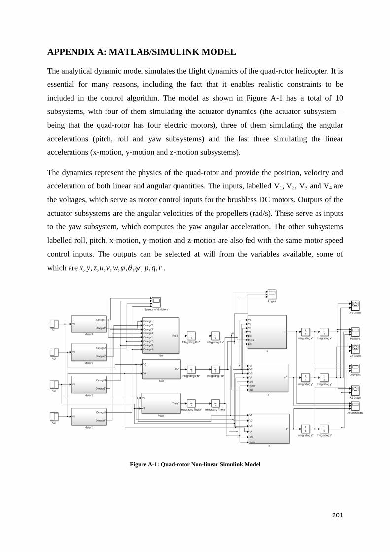
201
APPENDIX A: MATLAB/SIMULINK MODEL
The analytical dynamic model simulates the flight dynamics of the quad-rotor helicopter. It is
essential for many reasons, including the fact that it enables realistic constraints to be
included in the control algorithm. The model as shown in Figure A-1 has a total of 10
subsystems, with four of them simulating the actuator dynamics (the actuator subsystem –
being that the quad-rotor has four electric motors), three of them simulating the angular
accelerations (pitch, roll and yaw subsystems) and the last three simulating the linear
accelerations (x-motion, y-motion and z-motion subsystems).
The dynamics represent the physics of the quad-rotor and provide the position, velocity and
acceleration of both linear and angular quantities. The inputs, labelled V1, V2, V3 and V4 are
the voltages, which serve as motor control inputs for the brushless DC motors. Outputs of the
actuator subsystems are the angular velocities of the propellers (rad/s). These serve as inputs
to the yaw subsystem, which computes the yaw angular acceleration. The other subsystems
labelled roll, pitch, x-motion, y-motion and z-motion are also fed with the same motor speed
control inputs. The outputs can be selected at will from the variables available, some of
which are rqpwvuzyx ,,,,,,,,,,, ψθϕ .
Figure A-1: Quad-rotor Non-linear Simulink Model

202
In order to evaluate the model’s response to changes in voltage inputs, a 3-D visualization
system was included in the simulation system as shown in figure A-2. This allows for the
analysis of the position and the orientation of the quad-rotor, hence verifies its performance.
Figure A-2: 3-D simulation display
The figures A-1 and A-2 were used for all simulations within this thesis.
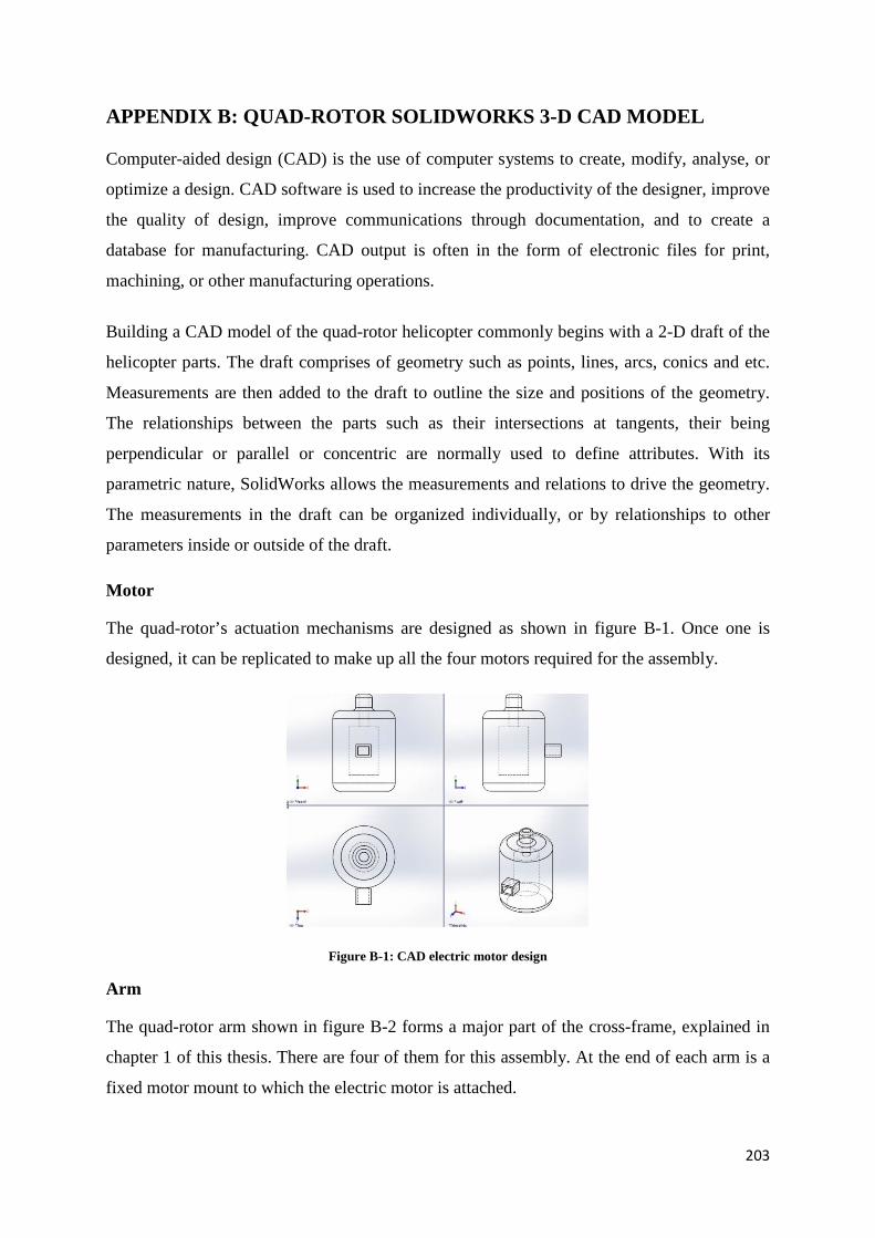
203
APPENDIX B: QUAD-ROTOR SOLIDWORKS 3-D CAD MODEL
Computer-aided design (CAD) is the use of computer systems to create, modify, analyse, or
optimize a design. CAD software is used to increase the productivity of the designer, improve
the quality of design, improve communications through documentation, and to create a
database for manufacturing. CAD output is often in the form of electronic files for print,
machining, or other manufacturing operations.
Building a CAD model of the quad-rotor helicopter commonly begins with a 2-D draft of the
helicopter parts. The draft comprises of geometry such as points, lines, arcs, conics and etc.
Measurements are then added to the draft to outline the size and positions of the geometry.
The relationships between the parts such as their intersections at tangents, their being
perpendicular or parallel or concentric are normally used to define attributes. With its
parametric nature, SolidWorks allows the measurements and relations to drive the geometry.
The measurements in the draft can be organized individually, or by relationships to other
parameters inside or outside of the draft.
Motor
The quad-rotor’s actuation mechanisms are designed as shown in figure B-1. Once one is
designed, it can be replicated to make up all the four motors required for the assembly.
Figure B-1: CAD electric motor design
Arm
The quad-rotor arm shown in figure B-2 forms a major part of the cross-frame, explained in
chapter 1 of this thesis. There are four of them for this assembly. At the end of each arm is a
fixed motor mount to which the electric motor is attached.
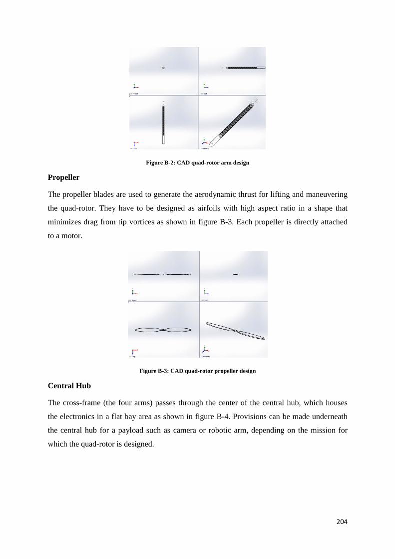
204
Figure B-2: CAD quad-rotor arm design
Propeller
The propeller blades are used to generate the aerodynamic thrust for lifting and maneuvering
the quad-rotor. They have to be designed as airfoils with high aspect ratio in a shape that
minimizes drag from tip vortices as shown in figure B-3. Each propeller is directly attached
to a motor.
Figure B-3: CAD quad-rotor propeller design
Central Hub
The cross-frame (the four arms) passes through the center of the central hub, which houses
the electronics in a flat bay area as shown in figure B-4. Provisions can be made underneath
the central hub for a payload such as camera or robotic arm, depending on the mission for
which the quad-rotor is designed.
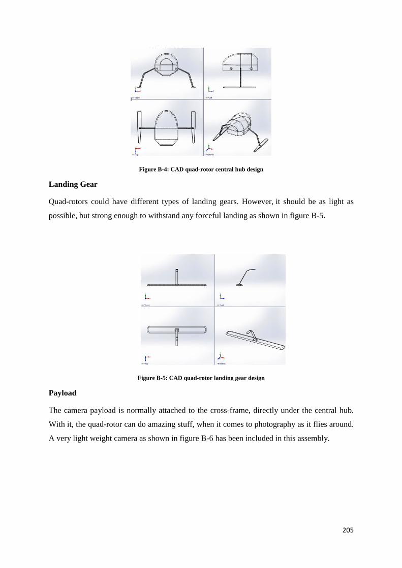
205
Figure B-4: CAD quad-rotor central hub design
Landing Gear
Quad-rotors could have different types of landing gears. However, it should be as light as
possible, but strong enough to withstand any forceful landing as shown in figure B-5.
Figure B-5: CAD quad-rotor landing gear design
Payload
The camera payload is normally attached to the cross-frame, directly under the central hub.
With it, the quad-rotor can do amazing stuff, when it comes to photography as it flies around.
A very light weight camera as shown in figure B-6 has been included in this assembly.
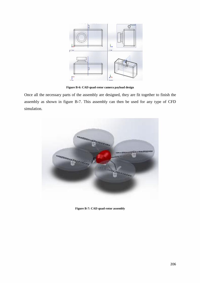
206
Figure B-6: CAD quad-rotor camera payload design
Once all the necessary parts of the assembly are designed, they are fit together to finish the
assembly as shown in figure B-7. This assembly can then be used for any type of CFD
simulation.
Figure B-7: CAD quad-rotor assembly

207
APPENDIX C: SAMPLE OF MODEL SIMULATION RESULTS
Throttle Command
MATLAB/ SIMULINK (outputs - motor speeds, angles and accelerations) SOLIDWORKS (output – forces) Motor Speeds (rad/s)
Angles (deg) Accelerations (m/s2) / Forces (N) [F = ma]
Forces (N) / Accelerations (m/s2) [𝑎 = 𝐹
𝑚 ]
Ω1 Ω2 Ω3 Ω4 𝜃 (Pitch)
φ (Roll)
ψ (Yaw)
X Y Z X Y Z
a F a F a F F a F a F a
226.2251 0 0 0 0 0 0 0 -0.0006 -0.0004 0 0 0 0 0 0 226.2251 226.2251 226.2251
226.2808 0 0 0 0 0 0 0 0.0055 0.0036 0 0 0 0 0 0 226.2808 226.2808 226.2808
230.4342 0 0 0 0 0 0 0 0.4697 0.3053 0 0 0 0 0.2200 0.3385 230.4342 230.4342 230.4342
241.2847 0 0 0 0 0 0 0 1.7597 1.1438 0 0 0 0 1.0563 1.6251 241.2847 241.2847 241.2847
251.8294 0 0 0 0 0 0 0 4.0486 2.6316 0 0 0 0 2.2247 3.4226 251.8294 251.8294 251.8294
262.0927 0 0 0 0 0 0 0 6.0851 3.9553 0 0 0 0 3.7024 5.696 262.0927 262.0927 262.0927
272.0961 0 0 0 0 0 0 0 9.3481 6.0763 0 0 0 0 5.7965 8.9177 272.0961 272.0961 272.0961
281.8584 0 0 0 0 0 0 0 11.0934 7.2107 0 0 0 0 6.8333 10.5128 281.8584 281.8584 281.8584
291.3961 0 0 0 0 0 0 0 15.502 10.0763 0 0 0 0 9.2430 14.2200 291.3961 291.3961 291.3961
300.7242 0 0 0 0 0 0 0 18.7938 12.2160 0 0 0 0 11.9826 18.4347 300.7242 300.7242 300.7242

208
Roll Command
MATLAB/ SIMULINK (outputs - motor speeds, angles and accelerations) SOLIDWORKS (output – forces) Motor Speeds (rad/s) Angles (deg) Accelerations (m/s2) / Forces (N)
[F = ma] Forces (N) / Accelerations (m/s2)
[𝑎 = 𝐹𝑚
]
Ω1 Ω2 Ω3 Ω4 𝜃 (Pitch
)
Φ (Roll
)
ψ (Yaw
)
X Y Z X Y Z
a F a F a F F a F a F a
227.6706
0 -2 0 0 0 0.3496
0.2272
0.1529
0.0994
0 0 0.1050
0.1615
0.0500
0.0769
227.6666
227.6706
227.6745
227.6706
0 -4 0 0 0 0.6988
0.4542
0.1346
0.0875
0 0 0.3902
0.6003
0.0460
0.0708
227.6627
227.6706
227.6785
227.6706
0 -6 0 0 0 1.0472
0.6807
0.1041
0.0677
0 0 0.5903
0.9082
0.0410
0.0631
227.6588
227.6706
227.6824
227.6706
0 -8 0 0 0 1.3943
0.9063
0.0615
0.0400
0 0 0.8307
1.2780
0.0386
0.0594
227.6548
227.6706
227.6863
227.6706
0 -10 0 0 0 1.7396
1.1307
0.0068
0.0044
0 0 0.9984
1.5360
0.0320
0.0492
227.6509
227.6706
227.6903
227.6706
0 -12 0 0 0 2.0877
1.3570
-0.060
9
-0.039
6
0 0 1.1092
1.7065
0.0294
0.0452
227.6469
227.6706
227.6943
227.6706
0 -14 0 0 0 2.4332
1.5816
-0.140
9
-0.091
6
0 0 1.4033
2.1590
0.0221
0.0340
227.6429
227.6706
227.6983
227.6706
0 -16 0 0 0 2.7756
1.8041
-0.233
1
-0.151
5
0 0 1.6542
2.5450
0.0183
0.0282
227.6389
227.6706
227.7023
227.6706
0 -18 0 0 0 3.1145
2.0244
-0.337
4
-0.219
3
0 0 1.8906
2.9086
0.0106
0.0163
227.6349
227.6706
227.7063
227.6706
0 -20 0 0 0 3.4496
2.2422
-0.453
6
-0.294
8
0 0 2.0973
3.2266
0.0050
0.0077
227.6309
227.6706
227.7103
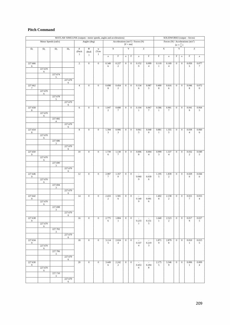
209
Pitch Command
MATLAB/ SIMULINK (outputs - motor speeds, angles and accelerations) SOLIDWORKS (output – forces) Motor Speeds (rad/s) Angles (deg) Accelerations (m/s2) / Forces (N)
[F = ma] Forces (N) / Accelerations (m/s2)
[𝑎 = 𝐹𝑚
]
Ω1 Ω2 Ω3 Ω4 𝜃 (Pitch
)
Φ (Roll
)
ψ (Yaw
)
X Y Z X Y Z
a F a F a F F a F a F a
227.6666
2 0 0 0.3496
0.2272
0 0 0.1529
0.0994
0.1101
0.1694
0 0 0.0505
0.0777
227.6706
227.6745
227.6706
227.6627
4 0 0 0.6988
0.4542
0 0 0.1346
0.0875
0.4008
0.6166
0 0 0.0468
0.0720
227.6706
227.6785
227.6706
227.6588
6 0 0 1.0472
0.6807
0 0 0.1041
0.0677
0.5861
0.9017
0 0 0.0419
0.0645
227.6706
227.6824
227.6706
227.6548
8 0 0 1.3943
0.9063
0 0 0.0615
0.0400
0.8811
1.3555
0 0 0.0394
0.0606
227.6706
227.6863
227.6706
227.6509
10 0 0 1.7396
1.1307
0 0 0.0068
0.0044
0.9993
1.5374
0 0 0.0322
0.0495
227.6706
227.6903
227.6706
227.6469
12 0 0 2.0877
1.3570
0 0 -0.060
9
-0.039
6
1.1955
1.8392
0 0 0.0290
0.0446
227.6706
227.6943
227.6706
227.6429
14 0 0 2.4332
1.5816
0 0 -0.140
9
-0.091
6
1.4028
2.1582
0 0 0.0217
0.0334
227.6706
227.6983
227.6706
227.6389
16 0 0 2.7756
1.8041
0 0 -0.233
1
-0.151
5
1.6401
2.5232
0 0 0.0179
0.0275
227.6706
227.7023
227.6706
227.6349
18 0 0 3.1145
2.0244
0 0 -0.337
4
-0.219
3
1.8719
2.8798
0 0 0.0101
0.0155
227.6706
227.7063
227.6706
227.6309
20 0 0 3.4496
2.2422
0 0 -0.453
6
-0.294
8
2.1755
3.3469
0 0 0.0061
0.0094
227.6706
227.7103
227.6706

210
Yaw Command
MATLAB/ SIMULINK (outputs - motor speeds, angles and accelerations) SOLIDWORKS (output – forces) Motor Speeds (rad/s)
Angles (deg) Accelerations (m/s2) / Forces (N) [F = ma]
Forces (N) / Accelerations (m/s2) [𝑎 = 𝐹
𝑚 ]
Ω1 Ω2 Ω3 Ω4 𝜃 (Pitch) φ (Roll)
Ψ (Yaw)
X Y Z X Y Z
a F a F a F F a F a F a
227.6761 0 0 2 0 0 0 0 0.1593 0.1035 0 0 0 0 0.2141 0.3294 227.6706 227.6761 227.6706
227.6817 0 0 4 0 0 0 0 0.1596 0.1037 0 0 0 0 0.2203 0.3389 227.6706 227.6817 227.6706
227.6872 0 0 6 0 0 0 0 0.1599 0.1039 0 0 0 0 0.2262 0.3480 227.6706 227.6872 227.6706
227.6928 0 0 8 0 0 0 0 0.1602 0.1041 0 0 0 0 0.2307 0.3549 227.6706 227.6928 227.6706
227.6983 0 0 10 0 0 0 0 0.1606 0.1044 0 0 0 0 0.2365 0.3638 227.6706 227.6983 227.6706
227.7039 0 0 13 0 0 0 0 0.1609 0.1046 0 0 0 0 0.2397 0.3688 227.6706 227.7039 227.6706
227.7094 0 0 15 0 0 0 0 0.1612 0.1048 0 0 0 0 0.2432 0.3742 227.6706 227.7094 227.6706
227.7150 0 0 17 0 0 0 0 0.1615 0.1050 0 0 0 0 0.2477 0.3811 227.6706 227.7150 227.6706
227.7205 0 0 19 0 0 0 0 0.1618 0.1052 0 0 0 0 0.2501 0.3848 227.6706 227.7205 227.6706
227.7261 0 0 21 0 0 0 0 0.1621 0.1054 0 0 0 0 0.2587 0.3980 227.6706 227.7261 227.6706

211
APPENDIX D: SAMPLE OF FLIGHT EXPERIMENT DATA
Time Height (mm)
Desired Output
Throttle value
Present X Position (mm)
Desired X Position (mm)
Present Y Position (mm)
Desired Y Position (mm)
2585031 219.1174 0 0 515.5879 500 1580.662 1600
2585265 219.0924 0 1 515.6742 500 1580.592 1600
2585281 219.0919 0 1 515.62 500 1580.614 1600
2585281 219.1135 0 1 515.6428 500 1580.645 1600
2585296 219.0887 0 1 515.6744 500 1580.665 1600
2585312 219.0981 0 1 515.5722 500 1580.62 1600
2585312 219.0916 0 1 515.6461 500 1580.588 1600
2585328 219.1592 0 1 515.528 500 1580.553 1600
2585343 219.1215 0 1 515.6463 500 1580.591 1600
2585343 219.0924 0 1 515.6204 500 1580.624 1600
2585359 219.1132 0 1 515.65 500 1580.608 1600
2585375 219.1233 0 1 515.6182 500 1580.613 1600
2585375 219.1382 0 1 515.6416 500 1580.623 1600
2585390 219.1029 0 1 515.6322 500 1580.611 1600
2585390 219.1822 0 1 515.4797 500 1580.528 1600
2585406 219.0802 0 1 515.6396 500 1580.665 1600
2585406 219.1087 0 1 515.5698 500 1580.675 1600
2585421 219.105 0 1 515.657 500 1580.675 1600
2585437 219.0765 0 1 515.5884 500 1580.695 1600
2585437 219.1335 0 1 515.6006 500 1580.604 1600
2585453 219.0795 0 1 515.6195 500 1580.579 1600
2585453 219.1057 0 1 515.5947 500 1580.635 1600
2585468 219.116 0 1 515.6479 500 1580.63 1600
2585468 219.1209 0 1 515.5812 500 1580.623 1600
2585484 219.1326 0 1 515.5894 500 1580.659 1600
2585500 219.123 0 1 515.6052 500 1580.66 1600
2585515 219.0897 0 1 515.6481 500 1580.617 1600
2585546 219.1044 0 1 515.5405 500 1580.621 1600
2585562 219.1317 0 1 515.5137 500 1580.59 1600
2585578 219.0905 0 1 515.5781 500 1580.63 1600
2585609 219.0806 0 1 515.6712 500 1580.673 1600
2585625 219.0942 0 1 515.6267 500 1580.619 1600
2585640 219.1425 0 1 515.5991 500 1580.627 1600
2585656 219.1053 0 1 515.612 500 1580.572 1600
2585687 219.1007 0 1 515.6479 500 1580.588 1600
2585703 219.1322 0 1 515.5644 500 1580.546 1600
2585718 219.0935 0 1 515.6012 500 1580.627 1600
2585750 219.0842 0 1 515.6346 500 1580.65 1600
2585765 219.1148 0 1 515.6503 500 1580.603 1600
2585781 219.1302 0 1 515.6143 500 1580.661 1600
2585796 219.1039 0 1 515.6277 500 1580.595 1600

212
Time Height (mm)
Desired Output
Throttle value
Present X Position (mm)
Desired X Position (mm)
Present Y Position (mm)
Desired Y Position (mm)
2585828 219.0995 0 1 515.6162 500 1580.624 1600
2585843 219.1138 0 1 515.6106 500 1580.614 1600
2585859 219.0795 0 1 515.6521 500 1580.639 1600
2585890 219.1305 0 1 515.6695 500 1580.621 1600
2585906 219.1292 0 1 515.4652 500 1580.529 1600
2585921 219.105 0 1 515.5855 500 1580.65 1600
2585937 219.1133 0 1 515.6595 500 1580.646 1600
2585968 219.0318 0 1 515.5965 500 1580.704 1600
2585984 219.1322 0 1 515.5838 500 1580.617 1600
2586000 219.1443 0 1 515.6219 500 1580.663 1600
2586015 219.089 0 1 515.6021 500 1580.633 1600
2586046 219.0828 0 1 515.6451 500 1580.692 1600
2586062 219.0954 0 1 515.6476 500 1580.596 1600
2586093 219.1045 0 1 515.6026 500 1580.607 1600
2586109 219.1447 0 1 515.6112 500 1580.662 1600
2586125 219.0796 0 1 515.5681 500 1580.646 1600
2586140 219.126 0 1 515.6712 500 1580.589 1600
2586171 219.1075 0 1 515.5401 500 1580.638 1600
2586187 219.0887 0 1 515.5599 500 1580.583 1600
2586203 219.1071 0 1 515.6609 500 1580.699 1600
2586218 219.1234 0 1 515.6172 500 1580.631 1600
2586250 219.1455 0 1 515.5348 500 1580.56 1600
2586265 219.1215 0 1 515.6514 500 1580.57 1600
2586281 219.1678 0 1 515.5909 500 1580.567 1600
2586296 219.0992 0 1 515.6171 500 1580.66 1600
2586328 219.0724 0 1 515.5973 500 1580.67 1600
2586343 219.0947 0 1 515.5735 500 1580.61 1600
2586359 219.1184 0 1 515.5482 500 1580.614 1600
2586375 219.0874 0 1 515.642 500 1580.653 1600
2586406 219.0767 0 1 515.634 500 1580.659 1600
2586421 219.1213 0 1 515.6464 500 1580.61 1600
2586437 219.1294 0 1 515.5466 500 1580.647 1600
2586468 219.1288 0 1 515.6613 500 1580.644 1600
2586484 219.1143 0 1 515.677 500 1580.614 1600
2586500 219.0761 0 1 515.5826 500 1580.68 1600
2586515 219.0996 0 1 515.6128 500 1580.571 1600
2586546 219.0961 0 1 515.6142 500 1580.677 1600
2586562 219.1018 0 1 515.6105 500 1580.653 1600
2586578 219.1165 0 1 515.6464 500 1580.637 1600
2586609 219.1085 0 1 515.6709 500 1580.627 1600
2586625 219.0863 0 1 515.6895 500 1580.635 1600
2586640 219.0981 0 1 515.6568 500 1580.59 1600
2586656 219.1136 0 1 515.6312 500 1580.618 1600
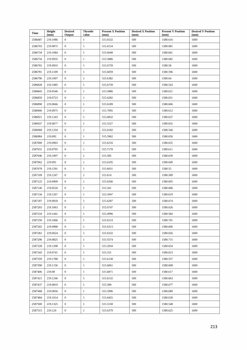
213
Time Height (mm)
Desired Output
Throttle value
Present X Position (mm)
Desired X Position (mm)
Present Y Position (mm)
Desired Y Position (mm)
2586687 219.1086 0 1 515.6532 500 1580.616 1600
2586703 219.0875 0 1 515.6154 500 1580.681 1600
2586718 219.1084 0 1 515.6049 500 1580.661 1600
2586734 219.0935 0 1 515.5886 500 1580.682 1600
2586765 219.0933 0 1 515.6729 500 1580.58 1600
2586781 219.1109 0 1 515.6059 500 1580.596 1600
2586796 219.1007 0 1 515.6382 500 1580.64 1600
2586828 219.1085 0 1 515.6739 500 1580.543 1600
2586843 219.0546 0 1 515.5886 500 1580.621 1600
2586859 219.0723 0 1 515.6282 500 1580.651 1600
2586890 219.0666 0 1 515.6189 500 1580.606 1600
2586906 219.0975 0 1 515.7095 500 1580.612 1600
2586921 219.1243 0 1 515.6832 500 1580.637 1600
2586937 219.0677 0 1 515.5527 500 1580.632 1600
2586968 219.1334 0 1 515.6182 500 1580.546 1600
2586984 219.092 0 1 515.5962 500 1580.656 1600
2587000 219.0903 0 1 515.6216 500 1580.632 1600
2587031 219.0795 0 1 515.7178 500 1580.611 1600
2587046 219.1007 0 1 515.585 500 1580.639 1600
2587062 219.091 0 1 515.6195 500 1580.649 1600
2587078 219.1591 0 1 515.6031 500 1580.55 1600
2587109 219.1247 0 1 515.614 500 1580.589 1600
2587125 219.0909 0 1 515.6566 500 1580.605 1600
2587140 219.0526 0 1 515.561 500 1580.686 1600
2587156 219.1267 0 1 515.5947 500 1580.619 1600
2587187 219.0918 0 1 515.6287 500 1580.674 1600
2587203 219.1063 0 1 515.6747 500 1580.626 1600
2587218 219.1441 0 1 515.4996 500 1580.584 1600
2587250 219.1066 0 1 515.6153 500 1580.701 1600
2587265 219.0988 0 1 515.6313 500 1580.606 1600
2587281 219.0624 0 1 515.6332 500 1580.656 1600
2587296 219.0825 0 1 515.5574 500 1580.715 1600
2587328 219.1308 0 1 515.5934 500 1580.634 1600
2587343 219.0741 0 1 515.551 500 1580.623 1600
2587359 219.1788 0 1 515.6138 500 1580.557 1600
2587390 219.1156 0 1 515.6061 500 1580.608 1600
2587406 219.08 0 1 515.6871 500 1580.617 1600
2587421 219.1246 0 1 515.6132 500 1580.663 1600
2587437 219.0819 0 1 515.589 500 1580.677 1600
2587468 219.0656 0 1 515.5996 500 1580.689 1600
2587484 219.1014 0 1 515.6455 500 1580.639 1600
2587500 219.1325 0 1 515.5158 500 1580.548 1600
2587515 219.124 0 1 515.6379 500 1580.625 1600

214
APPENDIX E: ADDITIONAL CONTROL SIMULATION RESULTS
No Wind Situation
In this situation, flows around the rotor blades of the helicopter are somewhat steady and the
rotors assumed to be working under the same conditions, because the wind speeds in the three
directions (x, y and z) were kept at 0m/s.
The vehicle follows the planned path, reaching the desired speed of 15m/s, having pitched
about 23 degrees. The controller is able to keep the helicopter flying at the commanded speed
and path without any deviation. As can be seen in the graphs in figure E-1, the velocity and
pitch angle remain constant throughout the 20 seconds flight, after reaching their commanded
values.
(a) Quad-rotor and wind speeds. (b) Roll and pitch angles.
Figure E-1: Graphs showing the helicopter parameters in a no wind situation
The curves that describe the speeds of each motor are as shown in figure E-2. Initially, the
quad-rotor was at stable hover and all the rotors spin at the same speed, taking it to the
reference height of 1 m. The controller then changes the speeds of motors 1 and 3 to create a
pitch angle to move the quad-rotor forward, while keeping motors 2 and 4 at a constant
speed. The quad-rotor reaches the commanded speed of 15m/s and experiences a stable cruise
with no disturbance. The speed and flight path of the helicopter are kept as commanded by
keeping speeds of the motors steady, after reaching the desired speed.

215
Figure E-2: Graph showing the speeds of the four motors of the quad-rotor in a no wind situation
Headwind
This study describes a situation where a constant wind opposes the flight of the quad-rotor. In
a constant headwind situation, the effects of the wind slamming the front of the quad-rotor
helicopter are seen from the graphs in figure E-3. After reaching the desired speed of 15m/s, a
constant headwind of speed 5m/s was introduced to oppose the forward flight of the
helicopter. The curves show an initial decline in the speed of the quad-rotor to 10m/s.
However, the action of the controller immediately tries to restore the speed of the helicopter
to the commanded value of 15m/s without success. The curve shows clearly that the
saturation block placed on the pitch angle, limits the quad-rotor to a maximum of 28 degrees
(as discussed in section 8.5 of chapter 8). Therefore it keeps to that restriction in the pitch
angle and only achieves a speed of 13.7 m/s. To make the quad-rotor regain its commanded
speed of 15 m/s, it needs to tilt more than 28 degrees, in which case the quad-rotor becomes
very unstable and difficult to control.

216
(a) Quad-rotor and wind speeds. (b) Roll and pitch angles.
Figure E-3: Graphs showing the helicopter parameters in a constant headwind
Figure E-4 shows how the controller compensates, by re-arranging the motor speeds to try to
nullify the effect of the disturbance. The robust controller increases the thrust from the rear
rotor by speeding up motor 3 and decreases that of the front rotor by slowing down motor 1
to take control of the situation, but because of the saturation limit, the speed of the quad-rotor
falls short by about 1.3 m/s.
Figure E-4: Graph showing the speeds of the four motors of the quad-rotor in a constant headwind
Tailwind
This simulation study describes a situation where a constant wind hits the quad-rotor from the
rear, increasing its speed and possibly making it deviate from the planned path. As the
vehicle has an induced speed due to the tail wind there is need to reduce the pitch angle, so as
to slow it down and keep it on course. The graphs in figure E-5 show oscillations in the quad-

217
rotor speed and pitch angle. Evidently, the speed of the quad-rotor is increased to a resultant
velocity of about 20 m/s. It is also clear that the pitch angle of the helicopter is slightly
increased, but the swift action of the controller reduces the pitch angle and restores the speed
to the commanded value of 15m/s, ensuring flight stability despite the tailwind effect.
(a) Quad-rotor and wind speeds. (b) Roll and pitch angles.
Figure E-5: Graphs showing the helicopter parameters in a constant tailwind
In compensating for the changes as a result of the tailwind, the controller re-arranges the
motor speeds to counter the effect of the wind and get it back to the commanded speed of
15m/s. Figure E-6 shows the motor speed curves. The robust controller decreases the thrust
from the rear rotor by slowing down motor 3 and increases that of the front rotor by speeding
up motor 1 to take control of the situation.
Figure E-6: Graph showing the speeds of the four motors of the quad-rotor in a constant tailwind

218
Crosswind
This simulation study describes a situation where the wind hits the quad-rotor from the side,
giving it a resultant speed and trying to make it deviate from the planned path. As shown in
graphs in figure E-7, the wind blows from the side of the helicopter causing a disturbance.
This disturbance creates a small roll angle, which tends to upset the helicopter. A resultant
speed, slightly higher than the commanded speed of 15m/s is reached. The action of the
controller creates a negative roll angle and a restoration of the speed of the helicopter as
commanded at the start of the flight.
(a) Quad-rotor and wind speeds. (b) Roll and pitch angles.
Figure E-7: Graphs showing the helicopter parameters in a constant crosswind
The motor speed curves in figure E-8 show the reaction of the controller when the
disturbance is encountered. A constant crosswind of speed 5m/s in introduced, blowing
eastwards from the side of the helicopter to try to make it veer off course. As a result of this
disturbance, the velocity of the quad-rotor is increased to a resultant velocity of 18.3m/s in
the NE direction as against the commanded speed of 15m/s. The robust controller is seen to
slow down and speed up the motors accordingly to take control of the situation.

219
Figure E-8: Graph showing the speeds of the four motors of the quad-rotor in a constant crosswind
220
APPENDIX F: LINEARIZATION OF QUAD-ROTOR MODEL
Taylor series approximation
The method used in the process of linearizing the quad-rotor non-linear dynamic system of
equations is Taylor series approximation. The approximation is done by representing a given
function with a series of terms calculated from the function’s derivatives at a single point
known as the operating point.
nn
xxn
xfxxxfxxxfxxxfxfxf )(!
)(...)(!3
)(''')(!2
)('')(!1
)(')()( 321 −++−+−+−+≈
In linearizing the system equations, the first order Taylor approximation is used, written as
))((')()(1
xxxfxfxfn
−+≈=
In the case of the quad-rotor the normal behaviour is when it is in stable hover. This implies
that the vehicle’s x-y body plane is parallel to the x-y earth plane, equivalent to a situation
when the vehicle’s roll, pitch and yaw angles are all equal to or close to zero. The operating
input voltage that corresponds to achieving the above conditions can be calculated from the
quad-rotor system equations. Here, all operating points are represented with subscript ‘h’.
( )( ) gVVVVk
kfm
Azq
t −+++
=
••
ϕθηρ coscos2 24
23
22
21
2
With
=======Ω=Ω
Ω=Ω=========
•••••••••
•••
•••••••••
00
0
zzyyxx
h
ψϕθψϕθψϕθ
Substituting the values of all the constants from the calibration table 4-1 (chapter 4) and the
conditions listed above, the following is obtained
( )( ) 81.90cos0cos0056.0
01.075.05.065.0
08042.01.120 24
23
22
21
2
−+++
××
××
= VVVV
( ) 81.9)44842.0)(27219.0(0 24
23
22
21 −+++= VVVV

221
( ) 81.912206.00 24
23
22
21 −+++×= VVVV
Here, it is assumed that all the motors behave in exactly the same way and the design of the
helicopter is symmetric; hence their voltage inputs at operating point are thought to be equal.
4321 VVVVVh ====
( ) 81.9412206.00 2 −×= hV
09333.20=hV
VoltsVh 48.4=
For this voltage, the speed with which the motors spin can be found at the operating point by
substituting using the equation 4-1, which describes the relationship between the motor speed
and voltage input.
qe
q kRDk
kJRV
2Ω+Ω+
Ω=
•
At the operating point voltage hV , let the motor speed be hΩ
2
0056.000000075.060.00015.0
0056.06.000006.0
Ω
×
+Ω+Ω
×
=•
hV
20000804.00015.000643.048.4 Ω+Ω+Ω=•
201250.023328.073406.696 Ω−Ω−=Ω•
Since the motor speeds remain constant at hover, •
Ω =0 and on substituting, the following
quadratic equation is obtained
001250.023328.073406.696 2 =Ω−Ω−
Using the almighty formula for solving quadratic equations,
aacbbx
242 −±−
=

222
)01250.0(2]73406.696)01250.0(4[)23328.0()23328.0( 2
−××−×−−±−−
=Ωh
025.089112.3423328.0
−±
=Ωh
025.089112.3423328.0
−+
=Ωh Or 025.0
89112.3423328.0−
−=Ωh
sradh /61.245−=Ω Or sradh /94.226=Ω
By discarding the negative root of the quadratic equation, the speed at operating voltage is
sradh /94.226=Ω
Linearization of Quad-rotor Equations
From the equation 20000804.00015.000643.0 Ω+Ω+Ω==•
VVh
Let A=0.00643, B=0.0015 and C=0.0000804
This leads to
2Ω+Ω+Ω=•
CBAV
Making •
Ω the subject of the formula gives
),(2 VfAC
AB
AV
Ω=Ω−Ω−=Ω•
First, the coefficients of the first order Taylor series have to be found.
ACB
AC
ABfL hh
h
Ω−−=
Ω−−=
Ω∂∂
=22~
AVfM
h
1~=
∂∂
=
VMLdtd
∆+∆Ω=∆Ω~~
)(
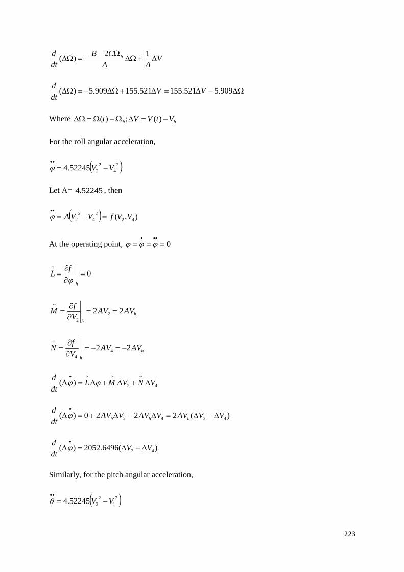
223
VAA
CBdtd h ∆+∆Ω
Ω−−=∆Ω
12)(
∆Ω−∆=∆+∆Ω−=∆Ω 909.5521.155521.155909.5)( VVdtd
Where hh VtVVt −=∆Ω−Ω=∆Ω )(;)(
For the roll angular acceleration,
( )24
2252245.4 VV −=
••
ϕ
Let A= 52245.4 , then
( ) ),( 422
42
2 VVfVVA =−=••
ϕ
At the operating point, 0===•••
ϕϕϕ
0~
=∂∂
=h
fLϕ
hh
AVAVVfM 22 2
2
~==
∂∂
=
hh
AVAVVfN 22 4
4
~−=−=
∂∂
=
4
~
2
~~)( VNVML
dtd
∆+∆+∆=∆•
ϕϕ
)(2220)( 4242 VVAVVAVVAVdtd
hhh ∆−∆=∆−∆+=∆•
ϕ
)(6496.2052)( 42 VVdtd
∆−∆=∆•
ϕ
Similarly, for the pitch angular acceleration,
( )21
2352245.4 VV −=
••
θ
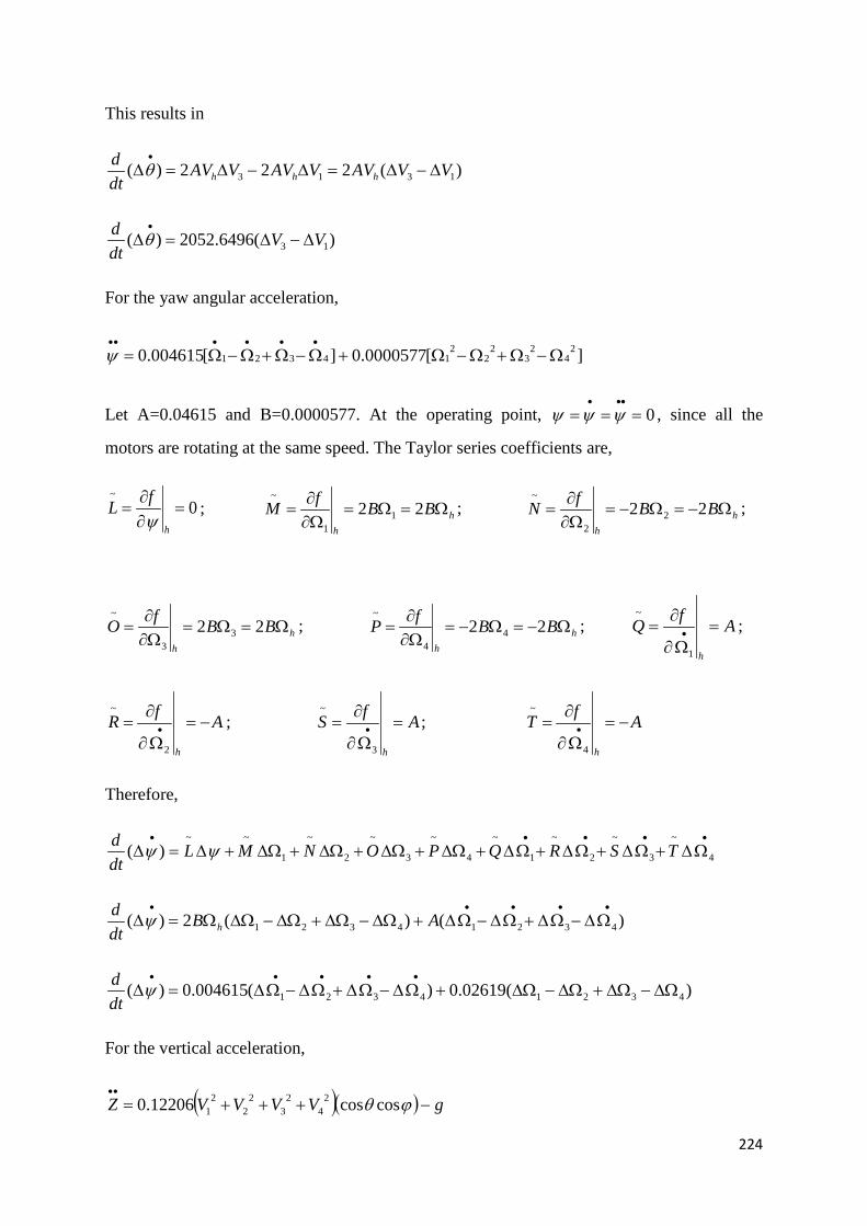
224
This results in
)(222)( 1313 VVAVVAVVAVdtd
hhh ∆−∆=∆−∆=∆•
θ
)(6496.2052)( 13 VVdtd
∆−∆=∆•
θ
For the yaw angular acceleration,
][0000577.0][004615.0 24
23
22
214321 Ω−Ω+Ω−Ω+Ω−Ω+Ω−Ω=
••••••
ψ
Let A=0.04615 and B=0.0000577. At the operating point, 0===•••
ψψψ , since all the
motors are rotating at the same speed. The Taylor series coefficients are,
0~
=∂∂
=h
fLψ
; hh
BBfM Ω=Ω=Ω∂∂
= 22 11
~; h
h
BBfN Ω−=Ω−=Ω∂∂
= 22 22
~;
hh
BBfO Ω=Ω=Ω∂∂
= 22 33
~; h
h
BBfP Ω−=Ω−=Ω∂∂
= 22 44
~; AfQ
h
=Ω∂
∂= •
1
~;
AfRh
−=Ω∂
∂= •
2
~; AfS
h
=Ω∂
∂= •
3
~; AfT
h
−=Ω∂
∂= •
4
~
Therefore,
•••••
Ω∆+Ω∆+Ω∆+Ω∆+∆Ω+∆Ω+∆Ω+∆Ω+∆=∆ 4
~
3
~
2
~
1
~
4
~
3
~
2
~
1
~~)( TSRQPONML
dtd ψψ
)()(2)( 43214321
•••••
Ω∆−Ω∆+Ω∆−Ω∆+∆Ω−∆Ω+∆Ω−∆ΩΩ=∆ ABdtd
hψ
)(02619.0)(004615.0)( 43214321 ∆Ω−∆Ω+∆Ω−∆Ω+Ω∆−Ω∆+Ω∆−Ω∆=∆•••••
ψdtd
For the vertical acceleration,
( )( ) gVVVVZ −+++=••
ϕθ coscos12206.0 24
23
22
21

225
At operating point, it is assumed that all the angles are small or very close to 0 and so their
cosines are approximately 1. Also, the vertical acceleration and velocity are 0, since the
altitude of the vehicle is not changing.
Let A=0.12206
( )( ) ),,,(coscos 43212
42
32
22
1 VVVVfgVVVVAZ =−+++=••
ϕθ
The coefficients are
0~
=∂∂
=hZ
fL ; hh
BVAVVfM 22 1
1
~==
∂∂
= ; hh
AVAVVfN 22 2
2
~==
∂∂
= ;
hh
AVAVVfO 22 3
3
~==
∂∂
= ; hh
AVAVVfP 22 4
4
~==
∂∂
=
4
~
3
~
2
~
1
~~)( VPVOVNVMZLZ
dtd
∆+∆+∆+∆+∆=∆•
)(2)( 4321 VVVVAVZdtd
h ∆+∆+∆+∆=∆•
)(0937.1)( 4321 VVVVZdtd
∆+∆+∆+∆=∆•
Linearized Quad-rotor Model
The Simulink model of the linearized quad-rotor system is based on the equations below. The
inputs of this model are the voltage control input of the motors whereas the output signals are
the roll, pitch and yaw angular acceleration and the vertical acceleration.
∆Ω−∆=∆Ω 909.5521.155)( Vdtd
)(6496.2052)( 42 VVdtd
∆−∆=∆•
ϕ
)(6496.2052)( 13 VVdtd
∆−∆=∆•
θ

226
)(02619.0)(004615.0)( 43214321 ∆Ω−∆Ω+∆Ω−∆Ω+Ω∆−Ω∆+Ω∆−Ω∆=∆•••••
ψdtd
)(0937.1)( 4321 VVVVZdtd
∆+∆+∆+∆=∆•
Transfer Functions of Linear Model
When the equations of motion are linearized the transfer function of quad-rotor plant can be
easily obtained by using the Laplace transform.
The Transfer function of the system, which presents the ratio of the output (angular velocity)
to the input (motor voltage).
∆Ω−∆=Ω•
909.5521.155 V
Using the Laplace transform gives
)(521.155)(909.5)( sVsss =Ω+Ω
)909.5(521.155
)()(
+=
ΩssV
s
Similarly the rest of the transfer functions of the linearized Quad-rotor model can be obtained
)(6496.2052 42 VV ∆−∆=••
ϕ
)]()([6496.2052)( 422 sVsVss −=ϕ
242
6496.2052)()(
)(ssVsV
s=
−ϕ
The same for the linearized pitch motion equation
213
6496.2052)()(
)(ssVsV
s=
−θ
For the yaw angular acceleration,
)(02619.0)(004615.0 43214321 ∆Ω−∆Ω+∆Ω−∆Ω+Ω∆−Ω∆+Ω∆−Ω∆=••••••
ψ

227
)]()()()([02619.0)]()()()([004615.0)( 432143212 ssssssssssssss Ω−Ω+Ω−Ω+Ω−Ω+Ω−Ω=ψ
)]()()()([02619.0)]()()()([004615.0)( 432143212 sssssssssss Ω−Ω+Ω−Ω+Ω−Ω+Ω−Ω=ψ
)]()()()()[02619.0004615.0()( 43212 sssssss Ω−Ω+Ω−Ω+=ψ
24321
)02619.0004615.0()]()()()([
)(ss
sssss +
=Ω−Ω+Ω−Ω
ψ
Since )()909.5(
521.155)( sVs
s+
=Ω , then
)()909.5(
)073.4718.0()()909.5(
)073.4718.0()()909.5(
)073.4718.0()()909.5(
)073.4718.0()( 42322212 sVss
ssVss
ssVss
ssVss
ss+
+−
++
++
+−
++
=ψ
)(0937.1 4321 VVVVZ ∆+∆+∆+∆=••
)]()()()([0937.1)( 43212 sVsVsVsVsZs +++=
)(0937.1)(0937.1)(0937.1)(0937.1)( 42322212 sVs
sVs
sVs
sVs
sZ +++=
The transfer functions obtained can be implemented in Simulink and used to formulate any
type of controller for any quad-rotor helicopter.
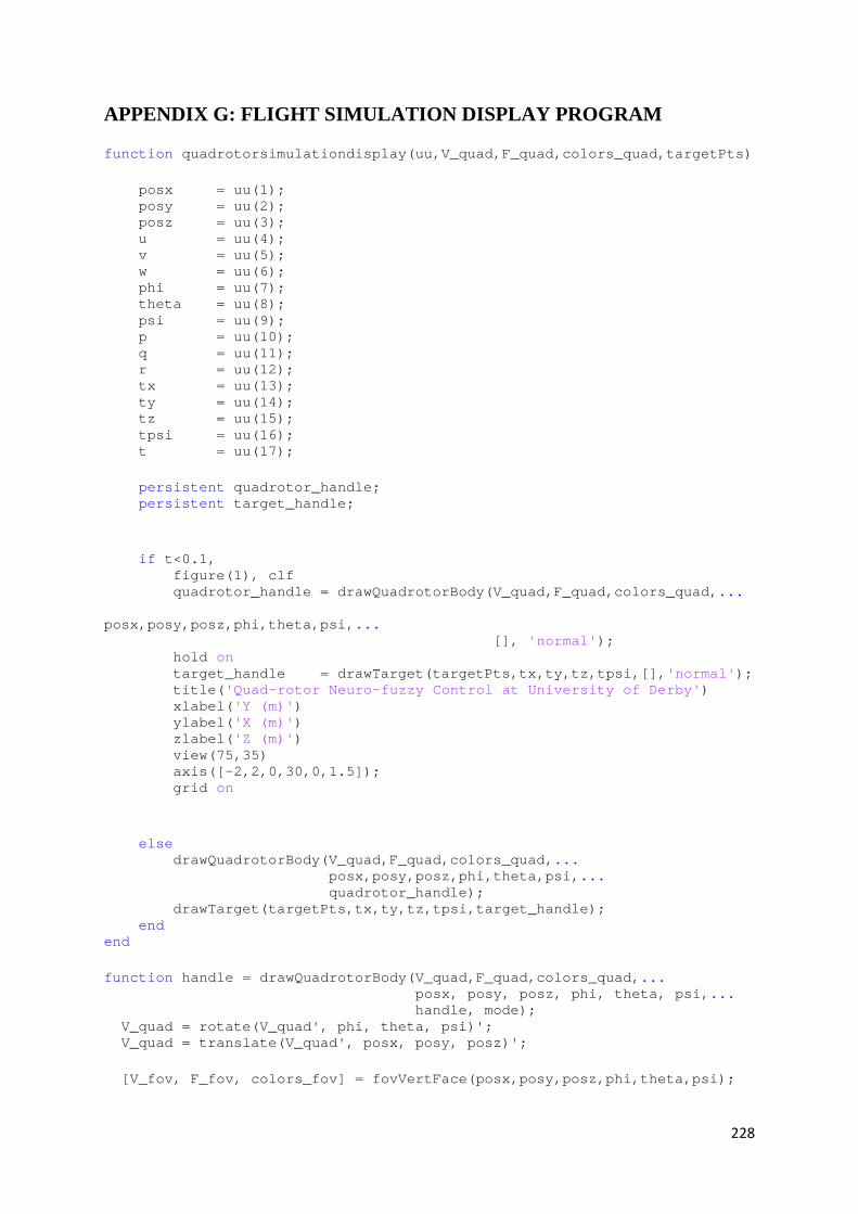
228
APPENDIX G: FLIGHT SIMULATION DISPLAY PROGRAM
function quadrotorsimulationdisplay(uu,V_quad,F_quad,colors_quad,targetPts) posx = uu(1); posy = uu(2); posz = uu(3); u = uu(4); v = uu(5); w = uu(6); phi = uu(7); theta = uu(8); psi = uu(9); p = uu(10); q = uu(11); r = uu(12); tx = uu(13); ty = uu(14); tz = uu(15); tpsi = uu(16); t = uu(17); persistent quadrotor_handle; persistent target_handle; if t<0.1, figure(1), clf quadrotor_handle = drawQuadrotorBody(V_quad,F_quad,colors_quad,... posx,posy,posz,phi,theta,psi,... [], 'normal'); hold on target_handle = drawTarget(targetPts,tx,ty,tz,tpsi,[],'normal'); title('Quad-rotor Neuro-fuzzy Control at University of Derby') xlabel('Y (m)') ylabel('X (m)') zlabel('Z (m)') view(75,35) axis([-2,2,0,30,0,1.5]); grid on else drawQuadrotorBody(V_quad,F_quad,colors_quad,... posx,posy,posz,phi,theta,psi,... quadrotor_handle); drawTarget(targetPts,tx,ty,tz,tpsi,target_handle); end end function handle = drawQuadrotorBody(V_quad,F_quad,colors_quad,... posx, posy, posz, phi, theta, psi,... handle, mode); V_quad = rotate(V_quad', phi, theta, psi)'; V_quad = translate(V_quad', posx, posy, posz)'; [V_fov, F_fov, colors_fov] = fovVertFace(posx,posy,posz,phi,theta,psi);
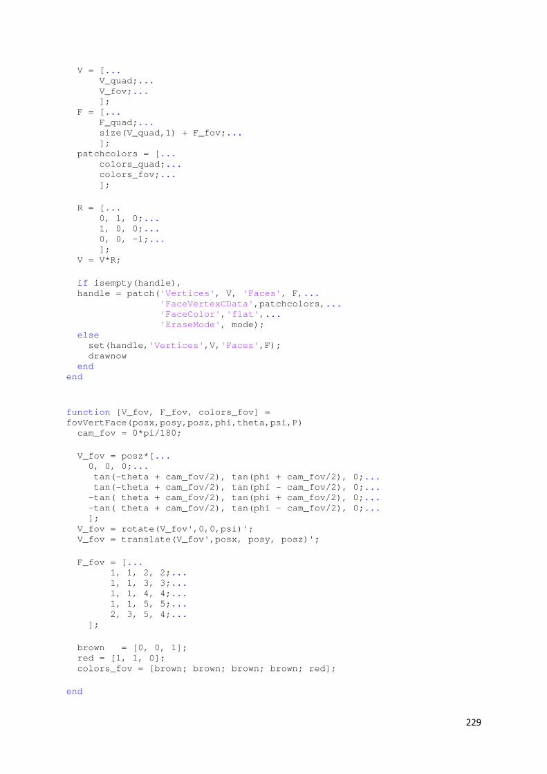
229
V = [... V_quad;... V_fov;... ]; F = [... F_quad;... size(V_quad,1) + F_fov;... ]; patchcolors = [... colors_quad;... colors_fov;... ]; R = [... 0, 1, 0;... 1, 0, 0;... 0, 0, -1;... ]; V = V*R; if isempty(handle), handle = patch('Vertices', V, 'Faces', F,... 'FaceVertexCData',patchcolors,... 'FaceColor','flat',... 'EraseMode', mode); else set(handle,'Vertices',V,'Faces',F); drawnow end end function [V_fov, F_fov, colors_fov] = fovVertFace(posx,posy,posz,phi,theta,psi,P) cam_fov = 0*pi/180; V_fov = posz*[... 0, 0, 0;... tan(-theta + cam_fov/2), tan(phi + cam_fov/2), 0;... tan(-theta + cam_fov/2), tan(phi - cam_fov/2), 0;... -tan( theta + cam_fov/2), tan(phi + cam_fov/2), 0;... -tan( theta + cam_fov/2), tan(phi - cam_fov/2), 0;... ]; V_fov = rotate(V_fov',0,0,psi)'; V_fov = translate(V_fov',posx, posy, posz)'; F_fov = [... 1, 1, 2, 2;... 1, 1, 3, 3;... 1, 1, 4, 4;... 1, 1, 5, 5;... 2, 3, 5, 4;... ]; brown = [0, 0, 1]; red = [1, 1, 0]; colors_fov = [brown; brown; brown; brown; red]; end

230
function handle = drawTarget(NED,tx,ty,tz,tpsi,handle,mode) NED = rotate(NED,0,0,tpsi); NED = translate(NED,tx,ty,tz); R = [... 0, 1, 0;... 1, 0, 0;... 0, 0, -1;... ]; XYZ = R*NED; if isempty(handle), handle = patch(XYZ(1,:), XYZ(2,:), XYZ(3,:), 'r', 'EraseMode', mode); else set(handle,'XData',XYZ(1,:),'YData',XYZ(2,:),'ZData',XYZ(3,:)); drawnow end end function XYZ=rotate(XYZ,phi,theta,psi); R_roll = [... 1, 0, 0;... 0, cos(phi), -sin(phi);... 0, sin(phi), cos(phi)]; R_pitch = [... cos(theta), 0, sin(theta);... 0, 1, 0;... -sin(theta), 0, cos(theta)]; R_yaw = [... cos(psi), -sin(psi), 0;... sin(psi), cos(psi), 0;... 0, 0, 1]; R = R_roll*R_pitch*R_yaw; XYZ = R*XYZ; end function XYZ = translate(XYZ,posx,posy,posz) XYZ = XYZ + repmat([posx;posy;posz],1,size(XYZ,2)); end

231
APPENDIX H: LIST OF PUBLICATIONS
The following journal paper was published during the course of the research work:
1. G. T. Poyi, M. H. Wu and A. Bousbaine. “Quad-rotor CFD Simulation and Analysis with
Artificial Neural Networks Error Compensation”, Applied Mechanics and Materials
(AMM) Journal (www.scientific.net), 2013.
The following journal papers have been completed and are in the process of publication:
1. G. T. Poyi, M. H. Wu, A. Bousbaine and H. Hu. “A Novel Approach to the Design of a
Robust Adaptive Controller for Quad-rotor Helicopters”.
2. G. T. Poyi, A. Bousbaine and M. H. Wu. “Design of an Intelligent Non-linear Fuzzy-
Neural Networks Controller for Quad-rotor Helicopters”.
3. G. T. Poyi, M. H. Wu and A. Bousbaine. “Artificial Neural Network Based Validation for
Quad-rotor Helicopter Simulink and SolidWorks Models”.
4. G. T. Poyi, M. H. Wu, A. Bousbaine and S. Sugiono. “CFD Model of a Quad-rotor
Helicopter for Dynamic Analysis”.
The following conference papers were written during the course of the research work:
1. G. T. Poyi, M. H. Wu and A. Bousbaine. “Quad-rotor Flight Simulation Error
Compensation using Artificial Neural Networks”, UPEC, Cluj-Napoca, Romania, 2014.
2. G. T. Poyi, M. H. Wu, A. Bousbaine, and B. Wiggins. “Validation of a Quad-rotor
Helicopter Matlab/Simulink and Solidworks Models”, IET Control and Automation
Conference, Birmingham 2013.
3. G. T. Poyi, M. H. Wu and A. Bousbaine. “Neuro-Fuzzy Control of the X4-flyer”,
Research snapshot presented at the East Midlands Universities conference, Derby 2013.
4. A. Bousbaine, M. H. Wu and G. T. Poyi. “Modelling and Simulation of a Quad-rotor
Helicopter”, 6th IET International Conference on Power Electronics, Machines and
Drives (PEMD), Bristol 2012.
5. G. T. Poyi, M. H. Wu and A. Bousbaine. “Modelling and CFD Simulation of a Quad-
rotor Helicopter”, Derby Electrical and Electronics Research Showcase 2012.
6. G. T. Poyi, M. H. Wu and A. Bousbaine. “Modelling and Control Simulation of a Quad-
rotor Helicopter”, University of Derby New horizons Post-graduate Research conference
2012.
232
7. G. T. Poyi, M. H. Wu and A. Bousbaine. “Neuro-Fuzzy Control of the X4-flyer”,
University of Derby New horizons Post-graduate Research conference 2012 (poster).
8. G. T. Poyi, M. H. Wu and A. Bousbaine. “A Novel Approach to the Control of the X-4
Flyer”, University of Derby New horizons Post-graduate Research conference 2011.
9. G. T. Poyi, M. H. Wu and A. Bousbaine. “A Novel Approach to the Control of the X-4
Flyer using Fuzzy-Neural Networks”, University of Derby Faculty of Arts Design and
Technology Research Conference 2011.