university of cincinnati center...university of cincinnati. he is the role model i wish to follow in...

UNIVERSITY OF CINCINNATI Date:___________________

I, _________________________________________________________, hereby submit this work as part of the requirements for the degree of:

in:

It is entitled:

This work and its defense approved by:

Chair: _______________________________ _______________________________ _______________________________ _______________________________ _______________________________

Creative Learning for Intelligent Robots

A dissertation submitted to the

Division of Research and Advanced Studies

of the University of Cincinnati

in partial fulfillment of the

requirements for the degree of

DOCTORATE OF PHILOSOPHY

in the Department of Mechanical, Industrial, and Nuclear Engineering

of the College of Engineering

2005

by Xiaoqun (Sherry) Liao

B.S. in Mech. Eng., Beijing Institute of Technology, 1990 M.S. in Mech. Eng., Beijing Institute of Technology, 1993

Committee Chair: Dr. Ernest L. Hall

ABSTRACT

This thesis describes a methodology for creative learning that applies to man and

machines. Creative learning is a general approach used to solve optimal control problems.

The theory contains all the components and techniques of the adaptive critic learning

family but also has an architecture that permits creative learning when it is appropriate.

The creative controller for intelligent machines integrates a dynamic database and a task

control center into the adaptive critic learning model. The task control center can function

as a command center to decompose tasks into sub-tasks with different dynamic models

and criteria functions, while the dynamic database can act as an information system. The

primary contribution of this work was merging the concepts of adaptive critics with a

dynamic database and task control center to create a new learning methodology called

creative control.

To illustrate ambiguousness of the theory of creative control, several experimental

simulations for robot arm manipulators and mobile wheeled vehicles were included. The

robot arm manipulator was one experimental example for testing the creative control

learning theory. The simulation results showed that the best performance was obtained by

using adaptive critic controller among all other controllers. By changing the paths of the

robot arm manipulator in the simulation, it was demonstrated that the learning component

of the creative controller was adapted to a new set of criteria. The Bearcat Cub robot was

another experimental example used for testing the creative control learning. The

kinematic and dynamic models of the Bearcat Cub were derived. Additionally, an optimal

PID control algorithm for WMR was developed to choose the parameters of the

controllers.

ii

The significance of this research was to generalize the adaptive control theory in a

direction toward highest level of human learning – imagination. In doing this it is hoped

to better understand the adaptive learning theory and move forward to develop more

human-intelligence-like components and capabilities into the intelligent robot. It is also

hoped that a greater understanding of machine learning will motivate similar studies to

improve human learning.

iii

To:

My two Jimmys

v

ACKNOWLEDGEMENTS

I am especially grateful to my advisor, Dr. Ernest L Hall, for his continued

guidance, encouragement and support through the whole period of my study at the

University of Cincinnati. He is the role model I wish to follow in my professional and

personal life, because of his creativity, wisdom, integrity, and best of all, his father-figure

kindness. Thanks to him, my graduate experience has gone beyond any of my dreams and

expectations I had as a student. It’s been an honor and a privilege to be a student of his.

My special appreciation is also extended to Professor Dr. Richard L. Shell, for his

advice, wisdom and for being on my committee. I am also grateful to professors Dr.

Ronald L. Huston, Dr. William G. Wee, and Dr. Chia-Yung Han for serving as my

advisory committee members.

I owe a debt of gratitude to my friend Carol Wolper who has nurtured my

happiness and peace of mind all along. I thank my classmates and teammates at Robotics

Research Center at the University of Cincinnati, especially Masoud Ghaffari, who is

always helpful to me.

I wish to dedicate this thesis to the two men in my life who make any of my

accomplishments possible and more meaningful: my Jimmys. They are the joy of my life

and make me laugh all the time. I can’t imagine my life without them. My love and

appreciation for them is endless.

vi

Table of Contents

ABSTRACT........................................................................................................................ ii

CHAPTER 1 INTRODUCTION ........................................................................................ 1

1.1 Background and Motivation ................................................................................................................. 1

1.1.1 Artificial intelligence and neural networks.................................................................................... 2

1.1.2 Adaptive critic learning ................................................................................................................. 4

1.1.3 Motivation ..................................................................................................................................... 5

1.2 Research Objectives ............................................................................................................................. 6

1.3 Significance .......................................................................................................................................... 8

1.4 Contribution to the Current State of the Art ......................................................................................... 9

1.5 Research Methodology....................................................................................................................... 11

1.6 Thesis Organization............................................................................................................................ 13

CHAPTER 2 LITERATURE REVIEW ........................................................................... 15

2.1 Intelligent Control Theory and Neurocontroller ................................................................................. 16

2.1.1 Robot control strategies ............................................................................................................... 16

2.1.2 Neural controller.......................................................................................................................... 24

2.2 Learning Theory ................................................................................................................................. 28

2.2.1 Machine learning ......................................................................................................................... 28

2.2.2 Supervised learning ..................................................................................................................... 29

2.2.3 Unsupervised learning ................................................................................................................. 30

2.2.4 Reinforcement learning ............................................................................................................... 31

2.3 Dynamic Programming and Optimal Control..................................................................................... 34

CHAPTER 3 ADAPTIVE CRITIC DESIGNS ................................................................ 41

3.1 Adaptive Critic ................................................................................................................................... 41

3.2 Historical Research Review................................................................................................................ 43

3.3 Hierarchy of Adaptive Critic Family.................................................................................................. 45

3.3.1 Levels of adaptive critic family ................................................................................................... 45

vii

3.3.2 Heuristic dynamic programming (HPD)...................................................................................... 48

3.3.3 Dual heuristic programming (DHP) ............................................................................................ 52

3.3.4 Globalized dual heuristic programming (GDHP) ........................................................................ 55

CHAPTER 4 CREATIVE LEARNING ........................................................................... 58

4.1 Adaptive Critic and Creative Learning............................................................................................... 58

4.1.1 Creative learning concept ............................................................................................................ 58

4.1.2 An example for creative learning ................................................................................................ 60

4.2 Creative Learning Architecture .......................................................................................................... 63

4.2.1 Dynamic knowledge database (DKD) ......................................................................................... 65

4.2.2 Task control center (TCC) ........................................................................................................... 66

4.3 Creative Learning Controller (for intelligent robot control)............................................................... 69

4.4 Adaptive Critic System Implementation ............................................................................................ 70

4.4.1 Adaptive critic system and NN.................................................................................................... 70

4.4.2 A comparison of HDP, DHP ....................................................................................................... 72

4.5 Tuning Algorithm and Stability Analysis........................................................................................... 74

4.5.1 System stability ........................................................................................................................... 74

4.5.2 Creative controller and nonlinear dynamic system...................................................................... 77

4.5.3 Critic and action NN weights tuning algorithm........................................................................... 78

4.6 Creative Control Mobile Robot Scenarios.......................................................................................... 81

4.6.1 Scenarios...................................................................................................................................... 83

4.6.2 Task control center ...................................................................................................................... 84

4.6.3 Dynamic databases ...................................................................................................................... 85

4.6.4 Robot learning module ................................................................................................................ 86

4.7 Chapter Summary............................................................................................................................... 87

CHAPTER 5 CASE STUDIES –TWO-LINK ROBOT ARM MANIPULATORS......... 88

5.1 Robot Manipulators and Nonlinear Dynamics ................................................................................... 88

5.2 PD Computed-torque (CT) Controller................................................................................................ 94

5.3 PID CT Controller .............................................................................................................................. 97

viii

5.4 Digital CT Controller ....................................................................................................................... 100

5.5 Adaptive Controller .......................................................................................................................... 105

5.6 Neural Network Controller (NN controller) ..................................................................................... 111

5.6.1 NN controller structure.............................................................................................................. 111

5.6.2 NN approximation ..................................................................................................................... 114

5.6.3 Two-layer NN controller ........................................................................................................... 117

5.6.4 NN controller simulation results................................................................................................ 117

5.7 Adaptive Critic Controller ................................................................................................................ 121

5.7.1 Adaptive critic network system design...................................................................................... 123

5.7.2 Adaptive critic simulation results .............................................................................................. 129

5.8 Summary .......................................................................................................................................... 134

CHAPTER 6 BEARCAT MOBILE ROBOT................................................................. 136

6.1 Scenarios for Bearcat Cub Mobile Robot ......................................................................................... 136

6.2 Kinematics Model of Bearcat Cub Robot......................................................................................... 139

6.2.1 Bearcat cub robot description .................................................................................................... 139

6.2.2 Bearcat Cub kinematical model................................................................................................. 146

6.3 Dynamic Model of Bearcat Cub Robot ............................................................................................ 150

6.3.1 Dynamic analysis....................................................................................................................... 150

6.3.2 Calculation of Pseudo-inverse matrix........................................................................................ 155

6.3.3 Bearcat Cub dynamic model...................................................................................................... 158

6.4 Computed Torques Using MathCad and MatLab............................................................................. 162

6.4.1 Dynamic model verification using MathCad............................................................................. 162

6.4.2 Computed torques using Matlab................................................................................................ 171

6.5 Summary .......................................................................................................................................... 174

CHAPTER 7 CASE STUDIES-WHEELED MOBILE ROBOTS................................. 175

7.1 Simulation Architecture for WMR (Bearcat Cub)............................................................................ 175

7.2 PD CT Controller for WMR (Bearcat Cub)...................................................................................... 178

7.2.1 PD CT controller ....................................................................................................................... 178

ix

7.2.2 Simulation results ...................................................................................................................... 178

7.2.3 Conclusions ............................................................................................................................... 185

7.3 PID CT Controller for WMR (Bearcat Cub) .................................................................................... 186

7.3.1 PID CT controller ...................................................................................................................... 186


7.3.3 Conclusions ............................................................................................................................... 194

7.4 Digital CT Controller for WMR (Bearcat Cub)................................................................................ 194

7.4.1 Digital controller for WMR....................................................................................................... 194


7.4.3 Conclusions ............................................................................................................................... 198

7.5 Adaptive Controller for WMR (Bearcat Cub) .................................................................................. 199

7.5.1 Adaptive controller architecture ................................................................................................ 199


7.5.3 Conclusions ............................................................................................................................... 213

7.6 PID Selection by Optimization......................................................................................................... 214

7.6.1 Calculate the inverse of matrix M.............................................................................................. 215

7.6.2 Design an optimal PID controller .............................................................................................. 217


7.7 Summary .......................................................................................................................................... 222

CHAPTER 8 CONCLUSIONS ...................................................................................... 223

8.1 Summary .......................................................................................................................................... 223

8.2 Conclusions ...................................................................................................................................... 226

8.3 Recommendations for Future Research............................................................................................ 227

REFERENCES ............................................................................................................... 229

APPENDIX A 2-LINK ARM MANIPULATOR........................................................... 247

APPENDIX A 2-LINK ARM MANIPULATOR........................................................... 247

APPEDEX B STABILITY ANALYSIS ........................................................................ 270

x

List of Figures Figure 1. 1 The brain as a whole system is an intelligent controller (3)............................. 2

Figure 1. 2 Schematic of biological neuron (5) .................................................................. 4

Figure 1. 3 The Mars exploration rovers by NASA(10)..................................................... 7

Figure 1. 4 Research methodology ................................................................................... 12

Figure 2. 1 Controller decomposition in primary and secondary controllers ................... 17

Figure 2. 2 ANN topologies: (a) single-layer feedforward; (b) multilayer feedforward; (c)

multilayer recurrent................................................................................................... 18

Figure 2. 3 McCulloch and Pitts neuron ........................................................................... 20

Figure 2. 4 Manipulator system driven by primary controller and secondary PID

controller (14) ........................................................................................................... 25

Figure 2. 5 Idea of indirect inverse control (54) ............................................................... 26

Figure 2. 6 Supervised learning systems (SLS) (54) ........................................................ 30

Figure 2. 7 Reinforcement learning systems (RLS) (54).................................................. 33

Figure 2. 8 Concept of dynamic programming................................................................. 36

Figure 3. 1 Level 1: adaptive critic system (54) ............................................................... 46

Figure 3. 2 Action-dependent adaptive critic(54) ............................................................. 47

Figure 3. 3 Level 3: Heuristic dynamic programming(54) .............................................. 48

Figure 3. 4 Critic adaptation in HDP(8, 80)...................................................................... 51

Figure 3. 5 Action adaptation in HDP(8, 80).................................................................... 51

Figure 3. 6 Critic adaptation in DHP(3, 54)...................................................................... 53

Figure 3. 7 Action adaptation in DHP(3).......................................................................... 54

xi

Figure 3. 8 Critic’s adaptation in general GDHP design (80, 88)..................................... 56

Figure 3. 9 Illustration of critic network in a straightforward GDHP design (80, 88) ..... 57

Figure 4. 1 Structure of the adaptive critic controller (130) ............................................. 59

Figure 4. 2 Proposed creative learning algorithm structure.............................................. 64

Figure 4. 3 Decomposition of the creative learning structure........................................... 65

Figure 4. 4 Functional structure of dynamic database ...................................................... 66

Figure 4. 5 Decomposition of the structure of task control center.................................... 68

Figure 4. 6 Block diagram of creative controller.............................................................. 69

Figure 4. 7 Three-layer neural network ............................................................................ 71

Figure 4. 8 Adaptive critic feedback controller - control schema (114)........................... 78

Figure 4. 9 General control schema for mobile robot systems (142)............................... 82

Figure 4. 10 Simple urban rescue site.............................................................................. 83

Figure 4. 11 Mission decomposition diagram.................................................................. 85

Figure 4. 12 Semantic dynamic database structure........................................................... 85

Figure 5. 1 Two-link robot arm manipulator .................................................................... 93

Figure 5. 2 Two-link robot arm simulation model............................................................ 93

Figure 5. 3 Joint tracking errors using PD CT controller for sin(), cos() trajectories....... 95

Figure 5. 4 Actual and desired angles using PD CT controller (Kp=100, Kv=20) .......... 95

Figure 5. 5 Joint tracking errors using PD CT controller for sin(), cos() trajectories....... 96

Figure 5. 6 Actual and desired angles using PD CT controller (Kp=500, Kv=20) .......... 96

Figure 5. 7 Joint tracking errors using PID CT controller (Kp=2, Ki=1, Kd=1): Unstable

................................................................................................................................... 98

xii

Figure 5. 8 Actual and desired angles using PID CT controller (Kp=2, Ki=1, Kd=1):

Unstable .................................................................................................................... 98

Figure 5. 9 Joint tracking errors using PID CT controller (Kp=50, Ki=10, Kd=10)........ 98

Figure 5. 10 Actual and desired angles using PID CT controller (Kp=50, Ki=10, Kd=10

................................................................................................................................... 98

Figure 5. 11 Joint tracking errors using PID CT controller (Kp=100, Ki=5, Kd=5)........ 99

Figure 5. 12 Actual and desired angles using PID CT controller (Kp=100, Ki=5, Kd=5)99

Figure 5. 13 Joint tracking errors using PID CT controller (Kp=100, Ki=5, Kd=5)...... 100

Figure 5. 14 Actual and desired angles using PID CT controller (Kp=100, Ki=5, Kd=5)

................................................................................................................................. 100

Figure 5. 15 the flow chart for the digital CT controller simulation............................... 101

Figure 5. 16 Joint tracking errors using digital CT controller, T=20msec: Unstable ..... 102

Figure 5. 17 Desired vs. actual joint angles using digital CT controller, T=20msec...... 102

Figure 5. 18 Joint 1, 2 control torque using digital CT controller, T=20msec ............... 102

Figure 5. 19 Joint tracking errors using digital CT controller, T=100msec: Unstable ... 103

Figure 5. 20 Desired vs. actual joint angles using digital CT controller, T=100msec.... 103

Figure 5. 21 Joint 1, 2 control torque using digital CT controller, T=100msec ............. 103

Figure 5. 22 Joint tracking errors using digital CT controller, T=20msec ..................... 104

Figure 5. 23 Desired vs. actual joint angles using digital CT controller, T=20msec...... 104

Figure 5. 24 Joint 1, 2 control torque using digital CT controller, T=20msec ............... 104

Figure 5. 25 Adaptive controller (11) ............................................................................ 106

Figure 5. 26 Joint tracking errors using adaptive controller ........................................... 109

Figure 5. 27 Actual and desired angles using adaptive controller .................................. 109

xiii

Figure 5. 28 Mass estimates using adaptive controller ................................................... 109

Figure 5. 29 Joint tracking errors using adaptive controller ........................................... 110

Figure 5. 30 Actual and desired angles using adaptive controller .................................. 110

Figure 5. 31 Mass estimates using adaptive controller ................................................... 111

Figure 5. 32 The proposed neural network simulation structure .................................... 112

Figure 5. 33 NN Activation functions............................................................................ 114

Figure 5. 34 Tracking error without NN: Unstable......................................................... 119

Figure 5. 35 Actual and desired joint angles without NN............................................... 119

Figure 5.36 Tracking errors with one-layer NN ............................................................. 119

Figure 5.37 Desired and actual with one-layer NN ........................................................ 119

Figure 5. 38 Tracking error with two-layer NN (432) .................................................... 120

Figure 5. 39 Actual and desired joint angles with two-layer NN (432).......................... 120

Figure 5. 40 Tracking error with two-layer NN (432) .................................................... 121

Figure 5. 41 Actual and desired joint angles with two-layer NN (432).......................... 121

Figure 5. 42 Dual heuristic programming adaptive critic control design(139)............... 123

Figure 5. 43 DHP event flow during ∆t = tk+1 – tk. ......................................................... 125

Figure 5. 44 Critic network adaptation event flow during ∆t = tk+1 – tk. ........................ 126

Figure 5. 45 Action network adaptation event flow during ∆t = tk+1 – tk. ...................... 126

Figure 5. 46 Tracking error with Adaptive Critic Controller (tf=10sec)......................... 131

Figure 5. 47 Actual and desired joint angles with Adaptive Critic Controller (tf=10) ... 131

Figure 5. 48 Tracking errors with Adaptive Critic Controller (λ=10) ............................ 131

Figure 5. 49 Actual and desired joint angles with Adaptive Critic Controller (λ=10) ... 131

Figure 5. 50 Tracking errors with Adaptive Critic Controller (tf=3sec, kv=500, λ=100)133

xiv

Figure 5. 51 Actual and desired joint angles with Adaptive Critic Controller (tf=3 sec,

λ=100) ..................................................................................................................... 133

Figure 5. 52 Tracking error with AC .............................................................................. 134

Figure 5. 53 Actual and desired joint angles with AC.................................................... 134

Figure 6. 1 (a) Bearcat cub (b) Bearcat cub uncovered (147)......................................... 137

Figure 6. 2 Obstacles on the course (passage) (148) ...................................................... 138

Figure 6. 3 Orange and white construction drums, cones, pedestals and barricades in the

course ...................................................................................................................... 138

Figure 6. 4 Typical course (map) for navigation challenge (148) .................................. 139

Figure 6. 5 WMR position coordinates(150) .................................................................. 141

Figure 6. 6 Fixed wheel or steering wheel structure (149) ............................................. 142

Figure 6. 7 Castor wheel(149) ........................................................................................ 143

Figure 6. 8 Robot dynamic analysis (150, 151) .............................................................. 150

Figure 6. 9 Robot position in initial frame and robot frame ........................................... 151

Figure 6. 10 Dynamic analysis for the robot................................................................... 153

Figure 6. 11 Mass moment of inertia of a rectangular prism(150, 152) ......................... 159

Figure 6. 12 Mass moment of inertia of a thin disc (150, 152)....................................... 159

Figure 6. 13 Segway tire structure (154) ....................................................................... 160

Figure 6. 14 Robot position vectors................................................................................ 168

Figure 6. 15 The torques by mass component ................................................................ 169

Figure 6. 16 The torques by J component....................................................................... 169

Figure 6. 17 The torques by G (gravity) component ...................................................... 170

Figure 6. 18 The total torques of the robot motion controller ........................................ 170

xv

Figure 6. 19 Robot trajectory .......................................................................................... 171

Figure 6. 20 Computed torques – mass component........................................................ 172

Figure 6. 21 Computed component- J component (friction forces related).................... 172

Figure 6. 22 Computed torques – gravity component..................................................... 173

Figure 6. 23 Computed torques Tau1 and Tau2 ............................................................ 173

Figure 7. 1 Tracking errors for WMR with a PD CT controller, kp=kv=0: Unstable. .... 180

Figure 7. 2 Desired and actual trajectories for WMR with a PD CT controller, k =k =0.p v

................................................................................................................................. 180

Figure 7. 3 Tracking errors for WMR with a PD CT controller, , kp=2, kv=1: Unstable.

................................................................................................................................. 180

Figure 7. 4 Desired and actual trajectories for WMR with a PD CT controller, , kp=2,

kv=1. ........................................................................................................................ 180

Figure 7. 5 Tracking errors for WMR with a PD CT controller, kp=10, kv=1: Unstable.

................................................................................................................................. 181

Figure 7. 6 Desired and actual trajectories for WMR with a PD CT controller, kp=10,

kv=1. ........................................................................................................................ 181

Figure 7. 7 Tracking errors for WMR with a PD CT controller, kp=20, kv=10.: Unstable.

................................................................................................................................. 181

Figure 7. 8 Desired and actual trajectories for WMR with a PD CT controller, kp=20,

kv=10. ...................................................................................................................... 181


................................................................................................................................. 182

xvi

Figure 7. 10 Desired and actual trajectories for WMR with a PD CT controller, k =100,

k =10.

p

v ...................................................................................................................... 182

Figure 7. 11 Tracking errors for WMR with a PD CT controller, kp1=2, kv1=1, kp2=0,

kv2=10, kp3=2, and kv3=1. Unstable. ....................................................................... 183


k =1, k =0, k =10, k =2, and k =1.

p1

v1 p2 v2 p3 v3 ................................................................ 183


kv2=200, kp3=100, and kv3=50. Unstable. ............................................................... 183


k =7, k =20, k =200, k =100, and k =50.

p1

v1 p2 v2 p3 v3 ....................................................... 183


kv2=5, kp3=2000, and kv3=1000. Unstable. ............................................................. 184


k =7, k =10, k =5, k =2000, and k =1000.

p1

v1 p2 v2 p3 v3 ..................................................... 184

Figure 7. 17 Tracking errors for WMR with a PD CT controller, kp1=1000, kv1=400,

kp2=200, kv2=100, kp3=2000, and kv3=1000. Unstable. .......................................... 185


k =400, k =200, k =100, k =2000, and k =1000.

p1

v1 p2 v2 p3 v3 ........................................... 185

Figure 7. 19 Tracking errors for WMR with a PID CT controller, kp=1, kv=1, ki=1. (sin)

Unstable. ................................................................................................................. 187

Figure 7. 20 Desired and actual trajectories for WMR with a PID CT controller, , k =1,

k =1, k =1. (sin)

p

v i ...................................................................................................... 187

xvii


................................................................................................................................. 188

Figure 7. 22 Desired and actual trajectories for WMR with PID controller, kp=2, kv=3,

ki=1. (sin) ................................................................................................................ 188

Figure 7. 23 Tracking errors for WMR with a PID CT controller, kp=2, kv=3, ki=2 (sin).

Unstable. ................................................................................................................. 188

Figure 7. 24 Desired and actual trajectories for WMR with a PID CT controller, , k =2,

k =3, k =2 (sin).

p

v i ...................................................................................................... 188


Unstable. ................................................................................................................. 189

Figure 7. 26 Desired and actual trajectories for WMR with a PID CT controller, k =2,

k =20, k =1 (sin).

p

v i .................................................................................................... 189


Unstable. ................................................................................................................. 190


k =3, k =1 (sin).

p

v i ...................................................................................................... 190

Figure 7. 29 Tracking errors for WMR with a PID CT controller, kp=1, kv=1, ki=1.

Unstable. ................................................................................................................. 191


k =1, k =1..

p

v i .............................................................................................................. 191

Figure 7. 31 Tracking errors for WMR with a PID CT controller, kp=2, kv=3, ki=1. Stable

................................................................................................................................. 191

xviii


k =3, k =1..

p

v i .............................................................................................................. 191


Unstable. ................................................................................................................. 192


k =3, k =5..

p

v i .............................................................................................................. 192


Unstable. ................................................................................................................. 193


k =20, k =1..

p

v i ............................................................................................................ 193


Unstable. ................................................................................................................. 193


k =2, k =1..

p

v i .............................................................................................................. 193

Figure 7. 39 Tracking errors for WMR with a digital CT controller, kp=2, kv=1. (sin)

Unstable. ................................................................................................................. 195

Figure 7. 40 Desired and actual trajectories for WMR with a digital CT controller, k =2,

k =1. (sin)

p

v ................................................................................................................ 195

Figure 7. 41 Tracking errors for WMR with a digital CT controller, kp=2, kv=100. (sin)

Unstable. ................................................................................................................. 196


k =100. (sin)

p

v ............................................................................................................ 196

xix

Figure 7. 43 Tracking errors for WMR with a digital CT controller, kp=2, kv=1 Unstable.

................................................................................................................................. 197


k =1

p

v ......................................................................................................................... 197

Figure 7. 45 Tracking errors for WMR with a digital CT controller, kp=2, kv=100

Unstable. ................................................................................................................. 198


k =100

p

v ..................................................................................................................... 198

Figure 7. 47 Tracking errors for WMR with a digital CT controller, kp=50, kv=1

Unstable. ................................................................................................................. 198

Figure 7. 48 Desired and actual trajectories for WMR with a digital CT controller, ,

kp=50, kv=1 ............................................................................................................. 198

Figure 7. 49 Adaptive controller tracking errors (2, 3, 100). Unstable........................... 202

Figure 7. 50 Adaptive controller desired versus actual motion trajectories. (2, 3, 100). 202

Figure 7. 51 Adaptive controller parameters estimate. (2, 3, 100) ................................. 203

Figure 7. 52 Adaptive controller tracking errors (2, 3, 15). Unstable............................. 204

Figure 7. 53 Adaptive controller desired versus actual motion trajectories.(2, 3, 15).... 204

Figure 7. 54 Adaptive controller parameters estimate (2, 3, 15). ................................... 204

Figure 7. 55 Adaptive controller tracking errors. ........................................................... 206

Figure 7. 56 Adaptive controller desired versus actual motion trajectories.(2, 3, 100).. 206

Figure 7. 57 Adaptive controller parameters estimate. ................................................... 206

Figure 7. 58 Adaptive controller tracking errors. ........................................................... 207

Figure 7. 59 Adaptive controller desired versus actual motion trajectories.(2, 3, 1000) 207

xx


Figure 7. 61 Adaptive controller tracking errors. (5, 3 ,100) Unstable.......................... 209



Figure 7. 64 Adaptive controller tracking errors. (2, 5 ,10) Unstable............................. 211

Figure 7. 65 Adaptive controller desired versus actual motion trajectories.(2, 5, 10).... 211


Figure 7. 67 Adaptive controller tracking errors. (2, 5 ,100) Unstable........................... 213



Figure 7. 70 Optimal PID controller simulation diagram. .............................................. 218

Figure 7. 71 Bearcat Cub dynamic model for simulation (Simulink)............................. 219

Figure 7. 72 The robot trajectory in x direction.............................................................. 220

Figure 7. 73 The robot trajectory in y direction.............................................................. 221

Figure 7. 74 The robot trajectory in θ direction.............................................................. 221

xxi

List of Tables Table 5. 1 Robot arm parameters...................................................................................... 94

Table 5. 2 Simulation parameters for a PD CT controller. ............................................... 95

Table 5. 3 Simulation parameters for a PD CT controller. ............................................... 96

Table 5. 4 Adaptive controller simulation parameters for the two-link manipulator. .... 108

Table 5. 5 Neurocontroller simulation parameters for the two-link manipulator. .......... 118

Table 5. 6Neurocontroller controller parameters for the two-link manipulator. ............ 118

Table 5. 7 Neurocontroller controller parameters for the two-link manipulator ............ 120

Table 5. 8 Neurocontroller simulation parameters for the two-link manipulator. .......... 130

Table 5. 9 Design parameters for adaptive critic controller............................................ 130

Table 5. 10 Design parameters for adaptive critic controller.......................................... 132

Table 5. 11 Design parameters for adaptive critic controller.......................................... 133

Table 7. 1 Bearcat Cub robot parameters........................................................................ 179

Table 7. 2 Adaptive controller simulation parameters for WMR. .................................. 201



Table 7. 5 Adaptive controller simulation parameters for WMR navigation. ................ 207




Table 7. 9 Recommended adaptive controller parameters for WMR. ............................ 214

Table 7. 10 Optimization results for kp, ki, kv................................................................. 220

xxii

CHAPTER 1 INTRODUCTION

Learning is a most remarkable characteristic of intelligent human behavior. The

theory of learning machines has been studied for more than 30 years and especially in the

last decade. However, the number of successful robotics applications that have been

reduced to practice is extremely small. This thesis describes a methodology for creative

learning that applies to machines, and we hope, also to man. Creative learning is a

general approach used to solve optimal control problems in which the criteria changes in

time. The theory presented contains all the components and techniques of the adaptive

critic learning family, but also has an architecture that permits creative learning when it is

appropriate. The creative controller for intelligent machines integrates a dynamic

database and a task control center into the adaptive critic learning model. The task control

center can function as a command center to decompose tasks into sub-tasks with different

dynamic model and criteria functions, while the dynamic database can act as an

information system.

This chapter is arranged in the following way. In Section 1.1 research background

and motivation are addressed. The research objectives are discussed in Section 1.2.

Section 1.3 and 1.4 summarize the significance and contribution of this thesis,

respectively. The research methodology is presented in Section 1.5. Finally, the layout of

the thesis is outlined in Section 1.6.

1.1 Background and Motivation

Paul Werbos, who is noted for his major contributions of the backpropagation and

chain rule inventions, posed a question in a recent speech (1): “how can we develop

1

better general-purpose tools for doing optimization over time, by using learning and

approximation to allow us to handle larger-scale, more difficult problems?” This thesis

addresses his question with ‘brain-like’ creative learning architecture as shown in Fig.

1.1(2, 3). Artificial intelligence and artificial neural network are introduced as research

background since “learning and approximation” mentioned in his statement is directly

related to this research area.

Figure 1. 1 The brain as a whole system is an intelligent controller (3)

1.1.1 Artificial intelligence and neural networks

Intelligence is the most outstanding human characteristic. Intelligence is often

concentrated on the ability to adapt. However, intelligence also includes the ability to

learn. Finally, intelligence also generally means to adapt and learn in a creative manner.

Intelligence is still not totally understood and therefore has many varying definitions,

implied meanings, and levels of sophistication which may be found in the literature.

Many studies in Artificial Intelligence (AI) attempt to implement the capacity of learning

or understanding with a mathematical or computer algorithm. Research in Machine

Intelligence (MI) is directed toward designing new, useful, adaptive machines.

Action

Reinforcement

Sensory

2

Current researchers are attempting to develop intelligent robots. Hall (4) defines

an intelligent robot as one that responds to changes to its environment through sensors

connected to a controller. Much of the research in robotics has been concerned with

vision and tactile sensing. Artificial intelligence, or AI, programs using heuristic methods

have concentrated on the problem of adapting, reasoning, and responding to changes in

the robot's environment. For example, one of the most important considerations in using

a robot in a workplace is human safety. A robot equipped with sensory devices that

detects the presence of an obstacle or a human worker within its workspace and

automatically stops its motion or shuts itself down in order to prevent any harm to itself

or the human worker is an important current implementation in most robotics work cells.

Artificial neural networks process information similarly to how the human brain

does. The network is composed of a large number of highly interconnected processing

elements (neurons). ANN models offer an attractive paradigm for learning. They offer the

ability not only to learn to solve problems from examples but also to discover the

problem. These models achieve good performance via massively parallel nets composed

of non-linear computational elements, sometimes referred to as units or neurons. With

each neuron is associated a function, referred to as the neuron's activation function.

Similarly, a number, called its weight, is also associated with each connection between

neurons. These resemble the firing rate of a biological neuron and the strength of a

synapse (connection between two neurons) in the brain. A neuron's activation function

depends on the activations of the neurons connected to it and the interconnection weights.

Neurons are often arranged into layers. Input layer neurons have their activations

3

externally set as shown in Figure 1.2. The creative learning proposed in this thesis is

directly inspired by the biological neuron learning structure.

Receiving Neuron

Components of a neuron

Sending Neurons

The synapse

Figure 1. 2 Schematic of biological neuron (5)

1.1.2 Adaptive critic learning

Artificial neural networks (ANN) are widely used for the design and analysis of

adaptive, intelligent systems for a number of reasons including: potential for massively

parallel computation, robustness in the presence of noise, resilience to the failure of

components, amenability to adaptation and learning, and sometimes resemblance to

biological neural networks. Artificial neural network learning algorithms can be divided

into supervised learning and unsupervised learning:

• Supervised neural networks need an external "teacher" during the learning phase,

which comes before the recalling (utilization) phase.

• Unsupervised neural networks "learn" from correlations of the input.

According to many researchers, the learning paradigms can also be expanded in

reinforcement learning and adaptive critic learning to solve nonlinear dynamic system

designs. The foundations of the optimal nonlinear system design lie in the field of

4

Dynamic Programming (DP), which is perhaps the most general approach for solving

optimal control problems. Dynamic programming methods use the principle of optimality

to find an optimal solution in a general nonlinear environment (6). Adaptive Critics

Designs (ACDs) offer a unified method to deal with the intelligent controller’s

nonlinearity, robustness, and reconfiguration for a nonlinear dynamic system.

Perhaps the most critical aspects of ACDs are found in the implementation. The

simplest form of adaptive critic design, heuristic dynamic programming (HDP), uses a

parametric structure called an action network to approximate the control policy and a

critic network to approximate the future cost or cost-to-go. In practice, since the

parameters of this architecture adapt only by means of the scalar cost, HDP has been

shown to converge very slowly (7). An alternative approach referred to as dual heuristic

programming (DHP) has been proposed. Here, the critic network approximates the

derivatives of the future cost with respect to the state. It is proved that DHP is capable of

generating smoother derivatives and has shown improved performance when compared to

HDP (8, 9).

Intelligent robot control can benefit from ACDs. By using ACDs to estimate

unknown parameters in the dynamic model, more accuracy can be obtained. By changing

the changing criteria for solutions, more creative solution can be obtained.

1.1.3 Motivation

According to the literature review, most of the researchers focused their topic of

learning machines in a very narrow area. As proposed by Werbos(2, 3), this work is

trying to extend the research to more general and useful learning machines and to

understand machine learning structure better. The adaptive critic learning algorithms in

5

previous research related to artificial neural networks, dynamic programming, and

machine learning algorithms are the resemblance to the human learning structure.

However, in order to develop “brain-like intelligent control” (2), it is not enough

to just have the adaptive critic portion as mentioned above. Our human brains are

naturally gigantic information systems, which process all the data stored in them for us to

make decisions. The decision-making ability is a very complicated function for us to

understand. That is, our brains act as control command centers. Of course, our human

brains learn through sensory information and reinforcement. Thus, adaptive critic

learning originated from an artificial neural network can be closely related to human

learning. However, our human brain learning is a creative and imaginative behavior.

In this thesis a novel algorithm called creative learning is proposed. The structure

of creative learning methodology can be a brain-like learning control system. The

structure of creative learning combines all of the components of adaptive critic learning.

Furthermore, it is integrated in both decision-making and database theory. For instance, it

selects the criteria or critics for the different sub-tasks and shows how to choose the

criteria function or utility function, and how to memorize the experience as human-like

memories. All are concerns of the creative learning techniques. In this thesis, a creative

learning architecture is proposed with evolutionary learning strategies.

1.2 Research Objectives

The primary goal of this dissertation is to develop a creative learning control

system beyond the adaptive critic learning control. This theory is beyond the adaptive

controller in that the reinforcement comes from the learning machine rather than from an

external critic. Such an approach offers potential solutions to problems in which the

6

objective criteria are unknown or yet to be discovered. The creative learning should

integrate its learning kernel with a knowledge database and a decision-making control

system. The knowledge database provides information for the learning center and the

decision-making system can connect the unstructured environment to collect data and

decompose the mission into sub-tasks such as the Mars Exploration Rovers as shown in

Fig. 1.3.(10).

Figure 1. 3 The Mars exploration rovers by NASA(10)

Known as a most important optimal theory, the three advanced adaptive critic

methods are summarized, namely, heuristic dynamic programming (HDP), dual heuristic

programming (DHP), and global dynamic heuristic programming (GDHP) according to

its own “ladder.” Beyond the adaptive critic approach, a creative learning theory will be

developed. There are many uncertainties in this area, such as, how many grades of J

function derivatives to use and when to apply them to the action module, how to select

learning parameters and how to select optimal learning rates, even though there are well-

7

known theories developed. All of the main results and conclusions will be verified in

computer simulations.

The purpose of this research is to develop a general, useful and more intelligent

machine. This research is also a part of our longer-term intelligent mobile robot project.

An integration of this project into the intelligent robot controller will be analyzed and

implemented. The controller for the intelligent robots should be simulated by using the

creative learning controller.

1.3 Significance

Intelligent industrial and mobile robots may be considered proven technology in

structured environments. However, it is believed that to extend the operation of these

machines to more unstructured environments requires a new learning method. Both

unsupervised learning and reinforcement learning are potential candidates for these new

tasks. The adaptive critic method has been shown to provide useful approximations or

even optimal control policies to non-linear dynamic systems. The purpose of this research

is to explore the use of new learning methods that go beyond the adaptive critic method

for unstructured environments.

The application of the creative theory appears to not only be to mobile robots but

too many other forms of human endeavor, such as educational learning and business

forecasting. Reinforcement learning, such as the adaptive critic, may be applied to known

problems to aid in the discovery of their solutions. The significance of creative theory is

that it permits the discovery of the unknown problems, ones that are not yet recognized

but may be critical to survival or success.

8

This research should advance the state of the art in learning systems. Learning

systems are used in many areas of science already; however, learning has not been

implemented in many manufacturing applications. Rather than continuous improvements,

many operations are repeated the same wrong way time after time. The creative learning

could also lead to a new generation of intelligent systems that have more humanlike

creative behavior and permit continuous improvement.

The significance of this research is to better understand the adaptive critic

learning theory and move forward to develop more human-intelligence-like components

into the intelligent robot controller. Moreover, it should extend to other applications as

well. On the other hand, adaptive critic family HDP, DHP, GDHP are the present state of

knowledge in learning theory field based on dynamic programming (DP). Creative

learning is a more generalized style of DP beyond the current adaptive critic learning

theory. Eventually, it is predicted that the creative learning theory is going to be a real

“emotional” or “expectations” component of a “brain-like” intelligent system(3).

1.4 Contribution to the Current State of the Art

This thesis proposes a methodology for creative learning that applies to machines,

which can be a general approach used to solve optimal control problems. The algorithm,

which is beyond the currently accepted adaptive critic learning, contains all the

components and techniques of the adaptive critic learning family but also has an

architecture that permits creative learning when it is appropriate. The creative controller

for intelligent machines integrates a dynamic database and a task control center into the

adaptive critic learning model. The task control center can function as a command center

to decompose tasks into sub-tasks with different dynamic model and criteria functions,

9

while the dynamic database can act as an information system. One scenario for intelligent

machines can be an autonomous mobile robot in an unstructured environment.

The robot arm manipulator is one experimental example for testing the creative

control learning theory. According to the previous research, the simulation programs on

PD CT, PID CT, digital and adaptive controller are developed in order to compare the

results with the adaptive critic controller. The simulation of the controllers is conducted

by selecting different parameters to compute the torques for the motion of the

manipulator.

Furthermore, the neurocontroller and adaptive critic controller for the robot arm

manipulator are developed. By comparing the response of the trajectory of joint angles

and the tracking errors, it demonstrates that the adaptive critic controller generates the

best performance among all the control techniques such as digital control, adaptive

control, and neurocontrol. The simulation results show that the best performance is

obtained by using adaptive critic controller among all other controllers. By changing the

paths of the robot arm manipulator in the simulation, it is demonstrated that the learning

component of the creative controller is adapted to a new set of criteria. The simulation is

a key step to prove that the creative control algorithm based on adaptive critic learning is

more advanced than other control techniques.

From robot arm manipulators to mobile robots, it’s the state-of-the-art research in

the robotics field. The scenarios for the wheeled mobile robot- Bearcat Cub are

developed according to the IGVC contest. The Bearcat Cub robot is another experimental

example used for testing the creative control learning. At first, the scenarios for the

autonomous guided vehicle (AGV) are developed. Secondly, the kinematic and dynamic

10

models are derived and verified in order to develop the robot controller. Finally, a

simulation on the robot motion control is conducted and the simulation results are

discussed by using PD CT, PID CT, digital and adaptive controller for the Wheeled

Mobile Robot (WMR) - Bearcat Cub.

Additionally, an optimal PID control algorithm for WMR is developed to choose

the parameters of the controllers. By using MatLab Simulink, an optimization model for

the PID controller is developed and a set of values for PID controller parameters are

obtained.

The primary contribution of this work is merging the concepts of adaptive critics

with a dynamic database and task control center to create a new learning methodology

called creative control. The dynamic database contains a copy of the plant model, copies

of all partial derivatives required in training and criteria model. Triggering a change of

criteria is an important feature of the task control center. Such change can be triggered

internally or more naturally by changes from the environment.

1.5 Research Methodology

It is critical to take an optimal approach in order to guarantee a successful

research plan. In this study, a literature review, simulation, and a comparison and

contrasting of major methodologies are key parts of the research activities. The broad

literature review ensures a thorough understanding of dynamic programming, artificial

intelligence, neural networks and learning algorithms. A comparison of the classic neural

controller with the adaptive critic controller proved its advancement of adaptive critic

learning algorithm. Moreover, case studies are also a part of the thesis experimental work.

The implementation results above are simulated in MatLab. MatLab provides rich

11

internal functions on neural network training and matrix calculations with a capability to

develop an interface with some other structure language like C/C++. The simplified

methodology of the proposed research is described in Figure 1.4.

RReevviieeww tthhee lliitteerraattuurree

DDeevveelloopp ccrreeaattiivvee lleeaarrnniinngg sscchheemmaa

BBuuiilldd aaddaappttiivvee ccrriittiicc ssiimmuullaattiioonn mmooddeell HHDDPP,, DDHHPP aanndd iimmpplleemmeenntt iitt

Figure 1. 4 Research methodology

DDeevveelloopp ttaasskk ccoonnttrrooll cceenntteerr pprroottoottyyppee

DDeevveelloopp iinntteerrffaaccee bbeettwweeeenn aaddaappttiivvee ccrriittiicc mmooddeell aanndd tthhee ddaattaabbaassee pprroottoottyyppee

VVeerriiffyy tthhee aallggoorriitthhmm

aacccceeppttaabbllee rreessuullttNN

YY

DDeevveelloopp tthhee rroobboott mmooddeellss

DDeevveelloopp tthhee mmooddeell ffoorr tthhee ccoonnttrroolllleerrss

DDeevveelloopp tthhee mmooddeell ffoorr tthhee ccoonnttrroolllleerrss

SSiimmuullaattiioonn ffoorr WWMMRR

NN YY CCrreeaattiivvee lleeaarrnniinngg mmooddeell

EExxppeerriimmeennttaall ssttuuddiieess

SSiimmuullaattiioonn ffoorr rroobboott aarrmm mmaanniippuullaattoorr

DDeevveelloopp DDaattaabbaassee pprroottoottyyppee

12

1.6 Thesis Organization

The main body of the thesis is organized in seven chapters. Chapter 2 reviewed

the foundations of nonlinear adaptive control design. The proposed philosophy is

formalized by reviewing artificial intelligence, machine learning theory, dynamic

programming and by linking these classical techniques to the adaptive critic architecture

of choice, i.e., dual heuristic programming adaptive critics. This chapter provided a

theoretical framework and background of the proposed creative learning algorithm.

Chapter 3 provided a general introduction to adaptive critic learning techniques

that were specifically developed with the control design objectives in mind. A brief

definition is introduced and then followed with the historical research work review. The

hierarchy-level of adaptive critic learning techniques is explained in the end.

Chapter 4 explained the creative learning algorithm. The novel structure combines

all the adaptive critic components described in Chapter 4. The dynamic database is

embedded in the adaptive critic controller integrating with the task control center in the

schema. Then an experimental study on implementing the adaptive critic controller is

presented to verify the algorithm structure. Both the dynamic database and task control

center’s prototype will be constructed in this chapter. Finally, a well-established creative

learning controller will be developed.

Chapter 5 showed how to derive the 2-link robot arm manipulator dynamic

equations including the classic PD, PID, digital controller, adaptive controller and neural

controller. Furthermore, it presented a detailed example of the newly proposed creative

learning algorithm implementation. A comparison of results with the adaptive critic

13

control results is given. This comparison of performance to that of Lewis’s (11) and other

adaptive critic techniques showed the advantages of the creative controller.

Chapter 6 started with the scenarios for the Bearcat mobile robots as another

experiment. The kinematics and dynamic model of the mobile robot are derived. By

using MathCAD and MatLab, the computed torques of the dynamic model are plotted..

Chapter 7 presented the simulation results of Bearcat Cub robot. In this chapter,

the simulation architecture for the WMR motion controller is presented. The PD CT

controller, PID CT controller, digital CT controller and adaptive controller are developed

for Bearcat Cub WMR motion control. Moreover, an optimal PID controller is developed.

Chapter 8 summarized the results of this thesis and made a recommendation to

future research.

14

CHAPTER 2 LITERATURE REVIEW

The most important ability of the brain is the ability to learn over time how to

make better decisions in order to better maximize the goals of the organism. To

understand the human brain scientifically, one must have some suitable mathematical

concepts to model the system. Since the human brain makes decisions like a control

system, it is an example of an intelligent control system. The natural way to imitate the

capability of the human brain in engineering systems is to build systems which learn over

time how to make decisions which maximize some measure of success or utility over

some future time. An intelligent robot system is one of these engineering systems. In this

context, dynamic programming is important because it is the only exact and efficient

approach for maximizing a utility function over some future time, in a general situation,

where random disturbances and nonlinearities are expected. Adaptive (approximate)

dynamic programming is important because it provides both the learning capability and

the possibility of reducing the computational cost to an affordable level (12). The

appearances of artificial neural networks and machine learning algorithms make it

possible to build true intelligent control systems in the future.

This chapter is a literature review on intelligent systems, artificial neural networks

and machine learning algorithms. Intelligent control theory and the neurocontroller are

discussed in Section 2.1. Machine learning, including supervised learning, unsupervised

learning and reinforcement learning, are presented in Section 2.2. The fundamental

classic dynamic programming approach is addressed in Section 2.3.

15

2.1 Intelligent Control Theory and Neurocontroller

The learning of locomotion in an unknown environment is extremely difficult to

achieve by formal logic programming. However, typical robot applications in

manufacturing assembly tasks would require locating components and placing them in

random positions. Fortunately, Kohonen (13)suggests that a higher degree of learning is

possible with the use of neural computers. The intelligent robot is supposed to plan its

action in the natural environment, while at the same time performing non-programmed

tasks. Learning has not yet been applied to industrial robots to any major extent. This

limits the application of intelligent robots.

2.1.1Robot control strategies

One popular robot control scheme is computed-torque control or inverse-

dynamics control. Most robot control schemes found in robust, adaptive, or learning

control strategies can be considered special cases of computed-torque control. These

techniques involve the decomposition of the control design problem into two parts (14):

1. A primary controller, a feedforward (inner-loop) designed to track the desired

trajectory under ideal conditions.

2. A secondary controller, a feedback (outer-loop) designed to compensate for

undesirable deviations (disturbances) of the motion from the desired trajectory based

on a linearized model.

The primary controller compensates for the nonlinear dynamic effects and attempts to

cancel the nonlinear terms in the dynamic model. However, since the parameters in the

dynamic model of the robot are not usually exact, undesired motion errors are expected.

16

The secondary controller can correct these errors. Figure 2.1 represents the

decomposition of the robot controller showing the primary and secondary controllers.

controller

Secondary controller

RobotY

dY +

-

Sensors

+ +

τPrimary

Figure 2. 1 Controller decomposition in primary and secondary controllers

The human brain has been the model for information-processing device for many

researchers in the design of intelligent computers, or neural computers. Psaltis, et al.(15)

described the neural computer as a large interconnected mass of simple processing

elements, or artificial neurons. The functionality of this mass, called the artificial neural

network, is determined by modifying the strengths of the connections during the learning

phase.

Researchers interested in neural computers have been successful in

computationally intensive areas such as pattern recognition and image interpretation

problems. These problems generally involve the static mapping of input vectors into

corresponding output classes using a feedforward neural network. The feedforward

neural network is specialized for the static mapping problems. In the robot control

problem, nonlinear dynamic properties need to be dealt with and a different type of

neural network structure must be used. Recurrent neural networks have the dynamic

properties, such as feedback architecture, needed for the appropriate design of such robot

controllers.

17

Artificial Neural Networks

ANNs are highly parallel, adaptive and fault tolerant dynamical systems modeled

like their biological counterparts. The phrases "neural networks" or "neural nets" are also

used interchangeably in the literature, which refer to neurophysiology, the study of how

the brain and its nervous system work. ANNs are specified by the following definitions

(16).

Topology

This describes the networked architecture of a set of neurons. The sets of neurons

are organized into layers, which are then classified as either feedforward networks or

n e u r o n

o u t p u t o u t p u to u t p u t

n e u r o n

i n p u t

n e u r o n

i n p u ti n p u t

l a y e r l a y e r l a y e r

l a y e rl a y e rl a y e r

h i d d e n

l a y e r

h i d d e n

l a y e r

( a ) ( b ) ( c )

Figure 2. 2 ANN topologies: (a) single-layer feedforward; (b) multilayer feedforward; (c) multilayer recurrent

recurrent networks. In feedforward layers, each output in a layer is connected to an input

in the next layer. In a recurrent ANN, each neuron can receive as its input a weighted

18

output from other layers in the network, possibly including itself. Fig. 2.2 illustrates

three simple representations of the ANN topologies.

Neuron

In ANNs, a neuron is a computational element that defines the characteristics of

input/output relationships. A simple neuron is shown in Fig. 2.3, which sums N weighted

inputs (called activation inputs) and passes the result through a nonlinear transfer

function to determine the neuron output. Two nonlinear functions that are often used to

mimic biological neurons are the unit step function and the linear transfer-function. A

very common formula for determining a neuron's output is through the use of sigmoidal

(squashing) functions:

g(x) = (1 + e−kx), (2.1.1)

that has a range of (0,1), and

2g(x) = tanh(kx) that has a range of (-1,1).

For various values of the slope parameter, k, these functions are conti

derivatives at all points.

Learning Rules

Given a set of input/output patterns, ANNs can learn to classify t

optimizing the weights connecting the nodes (neuron) of the networks

algorithms for weight adaptation can be described as either supervised

learning or reinforcement learning. In supervised learning, the desire

neuron is known, perhaps by providing training samples. During supervi

network compares its actual response, which is the result of the tr

described above, with the training example. It then adjusts its wei

(2.1.

nuous and have

hese patterns by

. The learning

or unsupervised

d output of the

sed training, the

ansfer function

ght in order to

19

minimize the error between the desired and its actual output. In unsupervised training,

where there are no teaching examples, built-in rules are used for self-modification, in

order to adapt the synaptic weights in response to the inputs to extract features from the

neuron. Kohonen's self-organizing map is an example of unsupervised learning (17).

Reinforcement learning is also called adaptive critic learning, is addressed in next

section.

One of the first models of an artificial neuron was introduced in 1943 by

McCulloch and Pitts and is shown in Fig. 2.3. They proved that a synchronous network of

neurons (M-P network) is capable of performing the simple logical tasks (computations)

that are expected of a digital computer. In 1958, Rosenblatt introduced the "perceptron",

in which he showed how an M-P network with adjustable weights can be trained to

classify sets of patterns. His work was based on Hebb's model of adaptive learning in the

human brain (18), in which he stated the neuron's interconnecting weights change

continuously as it learns (19).

w0 x0

Figure 2. 3 McCulloch and Pitts neuron

x1

xn

g(.)w1

… output input

wn

∑

20

In 1960, Bernard Widrow introduced the ADALINE (ADAptive LINear

element), a single-layer perceptron, and later extended it to what is known as

MADALINE, multilayer ADALINE (20). In MADALINE, Widrow introduced the

steepest decent method to stimulate learning in the network. His variation of learning is

referred to as the Widrow-Hoff rule or delta rule.

In 1969, Minsky and Papert (21)reported on the theoretical limitations of the

single layer M-P network, by showing the inability of the network to classify the

exclusive-or (XOR) logical problem. They left the impression that neural network

research is a farce, and went on to establish the "artificial intelligence" laboratory at MIT.

Hence, the research activity related to ANNs was largely dormant until the early 1980s

when the work by Hopfield, an established physicist, on neural networks rekindled the

enthusiasm for this field. Hopfield's autoassociative neural network (a form of recurrent

neural network) solved the classic hard optimization problem (traveling salesman) (22).

Other contributors to the field, Steven Grossberg and Teuvo Kohonon, continued

their research during the seventies and early eighties. During these “quiet years”, Steven

Grossberg (23, 24)worked on the mathematical development necessary to overcome one

of the limitations reported by Minsky and Papert (21). Teuvo Kohonon (25) developed

the unsupervised training method, the self-organizing map. Later, Bart Kosko (26)

developed bi-directional associative memory (BAM) based on the works of Hopfield and

Grossberg. Robert Hecht-Nielson (27) pioneered the work on neurocomputing.

It wasn't until 1986 that the two-volume book, by McClleland and Rumelhart,

titled Parallel Distributed Processing (PDP), exploded the field of artificial neural

networks (28). In this book a new training algorithm, called the Backpropagation

21

method (BP), the gradient search technique was used to train a multilayer perceptron to

learn the XOR mapping problem described by Minsky and Papert [(21). Since then,

ANNs have been studied for both design procedures and training rules (supervised and

unsupervised). An excellent collection of theoretical and conceptual papers on neural

networks can be found in books edited by Vemuri (19), and Lau (29). Interested readers

can also refer to a survey of neural networks book by Chapnick (30)categorized by:

theory, hardware and software, and how-to books.

The backpropagation algorithm is probably the most popular technique in the

field of artificial neural networks. However, there is a great deal of confusion on what is

meant under the term “backpropagation”. For many researchers, backpropagation is

firmly connected with the well-known gradient descent method of training a network. For

us backpropagation is simply an efficient and exact method for calculating derivatives in

a network. Priority in deriving backpropagation in its very general form must be granted

to Werbos who proposed and tested it in his Ph.D. dissertation in 1974 (published as a

book in 1994) (7, 31, 32).

The multilayer feedforward networks, using the BP method, represent a versatile

nonlinear map of a set of input vectors to a set of desired output vectors on the spatial

context (space). During the learning process, an input vector is presented to the network

and propagates forward from input layers to output layers to determine the output signal.

The output signal vector is then compared with the desired output vector, resulting in an

error signal. This error signal is backpropagated through the network in order to adjust

the network's connecting strengths (weights). Learning stops when the error vector has

reached an acceptable (16).

22

Many studies have been undertaken in order to apply both the flexibility and the

learning ability of backpropagation to robot control on an experimental scale (33-35). In

a recent study, an ANN utilizing an adaptive step size algorithm based on random search

techniques, improved the convergence speed of the BP method for solving the inverse

kinematical problem for a two-link robot (36). The robot control problem is a dynamic

problem, while the BP method only provides a static mapping of the input vectors into

output classes, which limits its benefits. In addition, like any other numerical method,

this novel learning method has limitations, like a slow convergence rate, and a local

minimum. Attempts to improve the learning rate of BP have resulted in many new

approaches (37, 38). It is necessary to note that the most important behavior of the

feedforward networks using the BP method is its classification ability or the

generalization to fresh data rather than temporal utilization of past experiences.

A recurrent network is a multilayer network in which the activity of the neurons

flows both from input layer to output layer (feedforward), and also from the output layer

back to the input layer (feedback), in the course of learning (27, 39) In a recurrent

network, each activity of the training set (input pattern) passes through the network more

than once before it generates an output pattern, whereas in standard BP only the error

flows backward, not the activity. This network architecture can base its response to

problems on both spatial (space) and temporal (time) contexts (39, 40). Therefore, it has

potential to model time-dependent processes such as robotic applications.

It is evident that a recurrent network will require a more substantial memory in

simulation (more connections) than a standard BP. Recurrent network computing is a

complex method, with a great deal of record keeping of errors and activities at each time

23

phase. However, preliminary results indicate that they have the ability to learn extremely

complex temporal patterns where data is unquantified with very little preprocessing, i.e.

stock market prediction and Fourier transforms relationships (41). In feedforward

networks where the training process has no memory, each input is independent of the

previous input. It is advantageous, especially in repetitive dynamical systems, to focus

on the properties of the recurrent networks to design better robot controllers.

2.1.2 Neural controller

In order to design intelligent robot controllers, one must also provide the robot

with a means of responding to problems in both a temporal and spatial time context. It is

the goal of the robot researcher to design a neural learning controller to utilize the

available data from the repetition in robot operation. The neural learning controller,

based on the recurrent network architecture, has the time-variant feature that once a

trajectory is learned, it should learn a second one in a shorter time. A common controller

in feedback systems is a proportional integral derivative (PID) controller for the robot

arm manipulator systems as shown in Fig. 2.4(14). The inverse dynamics could be

replaced by a neural learning controller as the primary controller, that is, the time-variant,

recurrent network will provide the learning block, or primary controller, for the inverse

dynamics. The neural controller compares the desired trajectories xd(t) with the actual

trajectories x(t) and corrects for the errors in the trajectory tracking. The new trajectory

parameters are then combined with the error signal from the secondary PID controller

(feedback controller) for actuating the robot manipulator arm.

24

Primary Controller

Figure 2. 4 Manipulator system driven by primary controller and secondary PID controller (14)

Neural networks can be applied either as a system identification model or as a

control for the robot controller described in Figure 2.4. ANNs can be used to obtain the

system model identification that can be used to design the appropriate controller. Once

the real system model is available, they can also be used directly in design of the

controller (42). Neural network approaches to robot control are discussed in general by

Psaltis et al (15) and Yabuta and Yamada (43). These approaches can be classified as:

1. Supervised control, a trainable controller that, unlike the old teaching pendant,

allows responsiveness to sensory inputs. A trainable neuromorphic controller

reported by Guez and Selinsky (44)provides an example of a fast, real-time and

robust controller.

2. Direct inverse control is trained for the inverse dynamic of the robot. Kung and

Hwang (45)used two networks on-line in their design of the controller.

)(ˆ tu +

+

-

)(txd

)(tx

Inverse Dynamics

)(tu

P

I

D

Secondary Controller

)( tu d

)(tx Manipulator

+

25

3. Neural adaptive control, neural networks combined with adaptive controllers

result in greater robustness and the ability to handle nonlinearity. Narendra (Chen

et al) (46) reported the use of the BP method for a nonlinear self-tuning adaptive

controller classified as direct and indirect control as shown in Figure 2.5, known

as one of the two best-known practitioners of adaptive control in the world today.

Widrow(47) presented “adaptive inverse control” implemented by using

“adaptive filters”.

4. Backpropagation of utility involves information flowing backward through time.

Werbos's back-propagation through time is an example of such a technique(7, 31,

32, 48-52).

5. Adaptive critic method uses a critic evaluating robot performance during training.

This is a very complex method that requires more testing (53)

Figure 2. 5 Idea of indirect inverse control (54)

In the direct inverse control approach, the recurrent neural network will learn the

inverse dynamic of the robot in order to improve the controller performance. In such a

system, the neural network model replaces the primary controller shown in Figure 2.1. In

this approach, a secondary feedback controller will be used to teach the network initially.

Action Network

Error= (X-Xr)2

X(t+1) u(t)

Derivatives of Error (Backpropagated)

Desired State Xr(t+1)

Model Network

Actual State R(t)

26

As learning takes place, the neural network takes full control of the system. Kawato and

his research group were successful using this approach in trajectory control of a three

degree-of-freedom robot (55, 56). Their approach is known as feedback-error-learning

control. However, their neural network structure was simply the linear collection of all

nonlinear dynamic terms, or subsystems, in the dynamic motion equation. Learning was

used purely for estimating the subsystems. As the degrees of freedom increase, the

network size needs to increase in the order of n4. For example, for six degrees-of-

freedom, 942 subsystems are needed, compared with 43 for a robot with three degrees-of-

freedom. However, due to the parallel processing capability of the neural network, the

implementation of Kawato's method is still an attractive method.

Goldberg and Pearlmutter(23) have demonstrated the utility of the feedback-error-

learning approach for the motion control of the first two joints of the CMU DDArm II,

using temporal windows of measured positions as input to the network; the output of the

network is the torque vector. Newton and Xu (57) used this approach to control a

flexible space robot manipulator (SM2) in real-time. The trajectory tracking error was

reduced by 85% when compared to conventional PID control scheme. More recently,

Lewis et al.(58) developed an on-line neural controller, based on the robot passivity

properties (that the system cannot become unstable if the robot cannot create energy),

using a similar approach with good tracking results. The feasibility and performance of

the feedback-error-learning control with global asymptotic stability has also been

reported (59, 60). The design of a compact and generic recurrent network has shown

promising results in replacing the need for custom subsystems-type design such as the

27

one by Kawato's group(61). The proposed controller performs based on the systematic

design approach and the recurrent network's time-variant feature.

2.2 Learning Theory

Learning theory discusses the fundamental algorithms, including supervised

learning, unsupervised learning, reinforcement learning, dynamic programming and

backpropagation, which became cornerstones of adaptive critic learning.

2.2.1 Machine learning

Machine learning research studies how knowledge can be learned from

observations or experiences of an agent. By learning the necessary knowledge with an

additional degree of autonomy - an agent's behavior is completely determined by its own

experiences. The purpose of machine learning algorithms is to use observations

(experiences, data, patterns) to improve a performance element, which determines how

the agent reacts when it is given particular inputs. The performance element may be a

simple classifier trying to classify an input instance into a set of categories or it may be a

complete agent acting in an unknown environment. By receiving feedback on the

performance, the learning algorithm adapts the performance element to enhance its

capabilities.

Norbert Wiener, the father of cybernetics, presented a very general but structured

definition of learning or machine learning. An organized system may be said to be one

which transforms a certain incoming message into an outgoing message, according to

some principle of transformation. If the principle of transformation is subject to a certain

criterion of merit of performance, and if the method of transformation is adjusted so as to

28

tend to improve the performance of the system according to this criterion, the system is

said to learn(61, 62).

Learning involves a persistent change or memory, defined mathematically as (63):

Learning ≡ dW/dt ≠ 0 (2.2.1)

No learning takes place without assumptions. All learning methods can be classified into

two categories: supervised learning and unsupervised learning as discussed in the

following.

2.2.2 Supervised learning

Supervised learning is a method of learning with a “training set”, which acts as “a

teacher” and/or global information of inputs and outputs (64, 65). The training data

consist of many pairs of input/output training patterns. Therefore, the learning will

benefit from the assistance of the teacher. During the training process, given a new

training pattern, the weights may be updated to minimize the difference between the

desired and actual outputs for each input as shown in Figure 2.6 (54). To solve the

supervised learning problem, two steps are required: first, one must specify the topology

of the network and, second, one must specify the learning rules. Most algorithms for

supervised learning work on a comparison between the desired outputs and the response

of the network during the training process. There are also techniques where input-output

pairs are directly used to update the weights in the network(63). Error-correction learning

by(66), reinforcement learning(67-69) and stochastic learning are examples of supervised

learning.

The examples of classification and regression using supervised learning are as

followed. Given a set of inputs: (X1, X2, … , Xn), where Xi= (xi1, …, xid)T,

29

d=dimension(Xi) and the corresponding desired outputs [Y1, …, Yn], the network training

purpose is to learn a map or approximate a function f: X-> Y from the inputs to the X ε

to outputs Y ε such that:

Yi ≈ f (Xi), i =1, …, n (2.2.2)

Where n is the number of the training examples. Here the inputs and outputs may be

discrete or continuous.

u(t)

Figure 2. 6 Supervised learning systems (SLS) (54)

2.2.3 Unsupervised learning

The unsupervised learning paradigm, also referred to as self-organization, has no

explicit “teacher” to oversee the training process. The network training process is capable

of discovering the statistical patterns corresponding to its input space and can develop the

different modes of behavioral action to represent different groups of inputs(64). Hebbian

learning, competitive and cooperative learning are examples of unsupervised learning

(63). There are a number of possibilities of the outputs that an unsupervised learning

detects in the input data such as familiarity, principle component analysis, clustering,

prototyping, encoding and feature mapping. Hebbian learning rules or revised Oja’s rule

S L S outputs inputs

SLS may have internal dynamics and “memory” of earlier times t-1, etc.

Predicted X(t)

Actual X(t)

targets

30

is an example for unsupervised learning. The mathematical equation of the plain Hebbian

learning is as following:

∆wi = ηVξi (2.2.3)

Where ∆w is the weight vector updates, η is the learning rate, V is the output and ξ is a

particular input(70). Kohonen's self-organizing map is an example of unsupervised

learning (17).

A basic principle of unsupervised learning is competition: output units compete

among themselves for activation. As a result, in most competitive learning algorithms

only one output neuron is activated at any given time. This is achieved by means of a so

called winner-take-all operation, which has been found to be biologically plausible(70).

These techniques allow the implementation of very powerful feature extraction modules

for autonomous learning systems. Moreover, they have been widely used in clustering

tasks, data dimensionality reduction, data mining (data organization for exploration and

search), information extraction, density approximation, data compression, etc.

2.2.4 Reinforcement learning

Reinforcement learning (RL), sometimes called as “learning with a critic”, is a

form of supervised learning because the network does get some feedback from its

environment(70). On the other hand, RL is different from supervised learning method

which is learning from explicit input-output examples provided by a knowledgeable

external supervisor. A RL agent learns by receiving a reward or reinforcement from its

environment, without the aid of an intelligent “teacher” or any form of supervision other

than its own decision making policy. So, we can argue that RL is a form of unsupervised

learning. According to Sutton et al(69), RL is learning what to do - how to map situations

31

to actions, in order to generate the optimal actions leading to a maximal numerical reward

signal. In reinforcement learning, the agent receives an input and an evaluation (reward)

of the action selected by the agent, and the learning algorithm has to learn a policy which

maps inputs to actions resulting in the best performance. The two most important

distinguishing concepts behind reinforcement learning are trial and error search and

delayed reward. Another feature of reinforcement learning is that it has a goal-directed

agent interacting with an uncertain environment. This goal is to consider the whole

problem of learning system instead of sub-problems without addressing how they might

fit into a bigger picture.

There are two basic elements in reinforcement learning, which are the agent and

the environment. The agent must be able to sense the state of the environment to some

degree and must take actions to affect the state. The agent also must have goal or goals

relating to the situation or state of the environment. Beyond the agent and the

environment, Sutton et al(69) identified four main sub-elements to a reinforcement

learning (RL) system: a policy, a reward function, a value function, and, optionally, a

model of the environment. A policy determines the learning agent’s way of behaving

stochastically. A reward function defines the goal of the learning system, representing the

intrinsic desirability of the environmental state. A value function specifies what is good

in the long run. As predictions of the rewards, it is values that are most concerned when

making and evaluating decisions. The agent’s action choices are made based on value

judgments. The final element is a model of the environment to decide on a course of

action by considering future states before they are actually experienced(69). The

reinforcement learning systems structure is shown in Fig. 2.7(54).

32

External Environment

or “Plant”

“utility” or “reward” U(t) or reinforcement

u(t) X(t) R L S actions Sensor inputs

RLS may have internal dynamics and “memory” of earlier times t-1, etc.

Figure 2. 7 Reinforcement learning systems (RLS) (54)

There are three threads of reinforcement learning: learning by trial and error,

problems of optimal control, and temporal-difference (TD) methods. Trial and error is

one of the basic concepts of reinforcement learning. As for TD methods, at each time

step, the TD(λ) algorithm is applied to change the network's weights. The formula for the

weight change is as follows(69):

(2.2.4)

Optimal control problems and its solution using value functions and dynamic

programming is also called adaptive critic learning, which is the third thread and

addressed in next chapter.

One of the simplest and most frequently used reinforcement learning methods

called Q-learning (68, 71, 72). The main idea behind Q-learning is to estimated a real-

valued function Q=Q(x,a), which is the expected discounted sum of future rewards for

performing action a in state x and performing optimal action thereafter. The optimal

33

policy can then be expressed in terms of Q by noting that an optimal action for state x is

any action a that maximizes Q(x,a). Q(x,a) satisfies the following equation (69)[(72):

),(),(max[),(),( 11 tttattttt asQasQrasQasQ −++← ++ γα (2.2.5)

where in this case, Q, the learned value function, directly approximates Q*, the optimal

action-value function. The Q-learning example helps us to illustrate the main features of a

typical reinforcement learning system. It includes a critic, an actor and an environment or

plant to be controlled.

The reinforcement learning theory we are addressing here actually gone by many

different names (1). Sometimes it is called “reinforcement learning (RL),” as depicted in

Figure 2.7. Sometimes it is called “adaptive critics,” in honor of Widrow’s original paper

in 1973 (67). It was described by Werbos(53)as “approximate dynamic programming

(ADP)” at various times. More recently, Bertsekas and Tsitsiklis (73, 74) have called it

“neuro-dynamic programming (NDP).” Most recently of all, Powell (75, 76) has used the

term “adaptive dynamic programming” (ADP) for his recent work.

2.3 Dynamic Programming and Optimal Control

Dynamic programming (DP) algorithm first was proposed in Bellman(6). DP is

based on the principle of optimality. Bellman formulated it as follows:

“An optimal policy has the property that whatever the initial state and initial decision are,

the remaining decisions must constitute an optimal policy with regard to the state

resulting from the first decision” (p.83)..

Unlike other branches of mathematical programming, one cannot talk about an

algorithm that can solve all dynamic programming problems. Dynamic programming,

34

like the branch and bound approach, is a way of decomposing certain hard to solve

problems into equivalent formats that are more amenable to solution. Basically, what the

dynamic programming approach does solve a multi-variable problem by solving a series

of single variable problems. The essence of dynamic programming is Bellman's Principle

of Optimality.

The original Bellman equation of dynamic programming for adaptive critic

algorithm is presented as follows (77):

0)()1/()))1(())(),(((max))(( UrtRJtutRUtRJ

tu−+>+<+= (2.3.1)

where r and U0 are constants that are used only in infinite-time-horizon problems and

then only sometimes, and where the angle brackets refer to expected value. Regarding the

finite horizon problems, which we normally try to cope with, we can actually use Eq.

(2.3.1) (77)

)1/()))1(())(),(((max))(()(

rtRJtutRUtRJtu

+>+<+= (2.3.2)

Where in both Eq.(2.3.1), (2.3.2), J(.) is the cost-to-go or strategic utility function or

secondary utility function, R(.) is the actual state form, u(t) is action vector and U(.) is the

utility function or local cost. The goal of most optimal problems is to estimate J function

to obtain optimal solutions. The basic concept of all forms of dynamic programming can

be illustrated as shown in Figure 2.8 (1).

35

Model of Utility Reality (R) Function (U)

Dynamic Programming

Secondary Utility (J)

Figure 2. 8 Concept of dynamic programming

How does one choose utility function U(.)? In principle, there is no technical

solution since it is supposed to represent what we want the system to do for us. In

practice, we often try out a utility function, simulate the results, and discover that the

system really does give us what we ask for. In tracking applications, the utility function

may simply represent tracking error. Experience shows that it helps to use a nice smooth

measure of tracking error, in order to speed up the learning by the system.

How does dynamic programming work? The user provides a utility function and

a stochastic model of the plant to be controlled. The technical expert tries to solve the

Bellman equation for the chosen model and utility function to achieve the approximation

of J by picking the action vector u(t). That is, by estimating the J function, we obtain the

optimal solution (25). Werbos stated that “there is only one exact method for solving

problems of optimization over time, in the general case of nonlinearity with random

disturbance: dynamic programming (DP)(1)”

Bertsekas(78) and Naidu(79) explained how to use dynamic programming to

solve optimal control system. We interpret Naidu’s examples in the following. At first,

summary of the Hamilton-Jacobi-Bellman is explained starting from the statement of the

36

problem to the solution of the problem as shown in Table 2.1(79). And then a specific

example is given to discuss the dynamic programming and the optimal control problem.

Statement of the problem

Let consider the optimal control system, that is, the plant as:

)),(),(()( ttutxftx =& (2.3.3)

where x, u are actual state and control unconstrained variables respectively, and we want

to minimize the performance index (“the secondary utility”)(79):

∫+=ft

tff dtttutxVttxSJ

0

)),(),(()),(( , (2.3.4)

and is the terminal cost function, is the integral cost term,

the boundary conditions as x(t

)),(( ff ttxS ∫ft

t

dtttutxV )),(),((0

0)=x0 and tf and x(tf) are free, find the optimal control.

Solution of the problem

Step 1: Form the Pontryagin

)),(),(()()),(),((),),(),(( ** ttutxftJttutxVtJtutx xx′

+=Η (2.3.5)

Step 2: Minimize u(t)

0)( * =∂Η∂u

and obtain (2.3.6) )),(),(()( *** ttJtxhtu x=

Step 3: Using the results of step 2 in step 1, find the optimal H*:

(2.3.7) )),(),((),),,),((),(( ******** ttJtxtJtJtxhtx xxx Η=Η

Step 4: Solve HJB equations

0),),(()( *** =Η+ tJtxtJ xt , (2.3.8)

37

with the initial conditions x0 and the final conditions

)),(()),(( **ffff ttxSttxJ = (2.3.9)

Step 5: Substitute the solutions of J*from step 4 to evaluate J*x and substitute into the

expression for u*(t) of step 2, to obtain optimal control.

Table 2. 1 Procedure summary of HJB approach (79)

Now let’s use an example to explain the algorithm (79):

Given a first order system:

)()(2)( tutxtx +−=& (2.3.10)

and the performance index (PI)(79)

∫ ++=ft

f dttutxtxJ0

222 )]()([21)(

21 (2.3.11)

find the optimal control.

Comparing the present plant (2.3.10) and the PI (2.3.11) with the general formulation of

the plant (2.3.3) and the PI (2.3.4), respectively, we see that (79)

)(21)),(( 2

fff txttxS = )(21)(

21)),(),(( 22 txtuttutxV +=

) (2.3.12) ()(2)),(),(( tutxttutxf +−=

Now we can follow the procedure summarized in table 2.1(79).

• Step 1: Form the H function:

))()(2()(21)(

21

)),(),(()()),(),((),),(),((

22

**

tutxJtxtu

ttutxftJttutxVtJtutx

x

xx

+−++=

′+=Η

(2.3.13)

• Step 2: Minimize u(t):

38

0)( * =∂Η∂u

, and then 0)( =+ xJtu (2.3.14)

and solve

xJtu −=)(* (2.3.15)

Step 3: using the optimal control (2.3.13) and (2.3.15), form optimal H function as

xx JtxtxJ )(2)(21

21 22 −+−=Η (2.3.16)

Now using the previous relations, the H-J-B equation (2.3.8) becomes

0)(2)(21

21 22 =−+− xxt JtxtxJJ (2.3.17)

with boundary condition (2.3.9) as

)(21)),(()),(( 2

fffff txttxSttxJ == (2.3.18)

Step 4: In order to solve the H equation with (2.3.18), we guess the solution as

)()(21))(( 2 txtptxJ = (2.3.19)

where, p(t), the unknown function to be determined, has the boundary condition as

)()(21)(

21))(( 22

ffff txtptxtxJ == (2.3.20)

which gives us:

1)( =ftp (2.3.21)

Then using (2.3.19), we get

)()( txtpJ x = , )()(21 2 txtpJ t &= (2.3.22)

and leading to the optimal control (2.3.15), as

)()()( ** txtptu −= (2.3.23)

39

Using the optimal control (2.3.22) into the HJB equation (2.3.17), we have

0)()21)(2)(

21)(

21( 2*2 =+−− txtptptp& (2.3.24)

For any x*(t), the previous relation becomes

021)(2)(

21)(

21 2 =+−− tptptp& (2.3.25)

Using the boundary condition (2.3.21), Eq. (2.3.25) becomes

)(52

)(52

53531

5353)25()25(

)(f

f

tt

tt

e

etp

−

−

⎥⎦

⎤⎢⎣

⎡

+−

−

⎥⎦

⎤⎢⎣

⎡

+−

++−

= (2.3.26)

Step 5: Using the relation (2.3.26), we solve the optimal control (2.3.23).

Note: 25)( −=∞∞→ftp and the optimal control (2.3.23) is

)()25()( txtu −−= (2.3.27)

The example presents an alternate method of obtaining the closed-loop optimal

control, using principle of optimality and the Hamilton-Jacobi-Bellman (HJB) equation.

This is important from the practical point of view in implementation of the optimal

control (79). The main advantage offered by DP is that the suboptimal process becomes

much simpler than the original problem(78). Bertsekas(78) in his two-volume textbooks

developed in depth dynamic programming, a central algorithmic method for optimal

control, sequential decision making under uncertainty, and combinatorial optimization.

40

CHAPTER 3 ADAPTIVE CRITIC DESIGNS

Perhaps the most critical aspects of adaptive critic designs (ACDs) are found in

the implementation. The simplest form of adaptive critic design, heuristic dynamic

programming (HDP), uses a parametric structure called an action network to approximate

the control policy and a critic network to approximate the future cost or cost-to-go. In

practice, since the parameters of this architecture adapt only by means of the scalar cost,

HDP has been shown to converge very slowly (7). An alternative approach referred to as

dual heuristic programming (DHP) has been proposed. Here, the critic network

approximates the derivatives of the future cost with respect to the state. It is proved that

DHP is capable of generating smoother derivatives and has shown improved performance

when compared to HDP (8, 9). Researchers also proposed another structure of ACDs,

called Globalized Dual Heuristic Programming (GDHP). All the three types of ACDs are

discussed in the following (77, 80).

3.1 Adaptive Critic

As mentioned in Section 2.4, dynamic programming (DP) is the only approach for

sequential optimization applicable to general nonlinear, stochastic environments.

However, DP needs efficient approximate methods to overcome its dimensionality

problems. It is only with the presence of artificial neural network (ANN) and the

invention of backpropagation that such a powerful and universal approximate method has

become a reality. As shown in Eq. (2.3.2), dynamic programming gives the exact solution

to the problem of how to maximize a utility function U(R(t)) over the future times, t, in a

nonlinear stochastic environment, where the vector R(t) represents the state of the

41

environment at time t. Dynamic programming converts a difficult long-term problem in

optimization over time <U(R(t))>, the expected value of U(R(t)) over all the future times,

into a much more straightforward problem in simple, short-term function maximization –

after we know the function J. Thus, all of the approximate dynamic programming

methods discussed here are forced to use some kind of general-purpose nonlinear

approximate to the J function, the value function in the Bellman equation, or something

closely related to J(54).

In most forms of adaptive critic designs, researchers approximate J by using a

neural network. Therefore, J(R) can be approximated by some function , where

W is a set of weights or parameters, is called a Critic network(67, 81). If the weights

W are adapted or iteratively solved for, in real time learning or offline iteration, Critic is

called an Adaptive Critic(48). An adaptive critic design (ACD) is any system which

includes an adapted critic component; a critic, in turn, is a neural net or other nonlinear

function approximator which is trained to converge to the function J(X).

),(ˆ WRJ

J

In adaptive critic learning or designs, the critic network learns to approximate the

cost-to-go or strategic utility function J and uses the output of an action network as one of

its’ input, directly or indirectly. When the critic network learns, backpropagation of error

signals is possible along its input feedback to the action network. To the backpropagation

algorithm, this input feedback looks like another synaptic connection that needs weights

adjustment. Thus, no desired control action information or trajectory is needed as

supervised learning. All that is needed is a desired cost function J.

42

3.2 Historical Research Review

Werbos(1) classified dynamic programming specified in adaptive critic designs

into five disciplines, which are neural network engineering, control theory, computer

science or artificial intelligence, operations research and fuzzy logic or control. Since the

first early implementations in 1993, model based adaptive critic has outperformed other

modern control and neurocontrol methods in a variety of difficult simulated problems,

ranging from missile interception(82, 83) through to preventing cars from skidding when

driving over unexpected patches of ice(84) and communication networks (wireless

cellular networks) (85, 86). These are many successful research cases in each of the areas

as summarized in the following.

“Adaptive critic” in early stage

“Adaptive critic” was first shaped by Bernard Widrow (20, 67) in 1973. He had

originally proposed an adaptive linear element as we mentioned in previous section,

known as ADALINE, and later extended it to what is known as MADALINE, multilayer

ADALINE(20). He showed how it was able to learn a strategy of play for the game

blackjack, with a performance close to that of the known optimal strategy.

Further development has followed, and, by the beginning of the 1980s, two

neuron-like adaptive elements were successfully able to learn how to balance an inverted

pendulum on a cart, which is a modified version of the standard control benchmark(87).

However, it was not until 1990 that Werbos(7) synthesized backpropagation and adaptive

critics. Werbos called critics backpropagated adaptive critics. He also pioneered in the

research on dynamic programming(12, 32, 53, 81). It was also Werbos who proposed two

43

types of adaptive critics: model-based and action dependent and most importantly, a

hierarchy of adaptive critic designs discussed in next section.

Neurocontroller

Wunsch et al. devoted his research on adaptive critic based neurocontroller for

turbogenerators and extended to multiple generators on the power grid and other

applications(88-96). Venayagamoorthy (Kumar) joined Wunsch’s group and did

thorough research on neurocontroller for turbogenerators based on adaptive critic

designs(90, 94, 96-98) and for other industrial applications(99, 100). Prokhorov(80) did

his dissertation on adaptive critic designs and their applications, known as a synthetic

development of generalizing various key results in the area of adaptive critics for the last

quarter century. Balakrishnan et al (82, 101-103) studied adaptive-critics for control of

nonlinear and distributed parameter systems such as nonlinear flight control. Si et al.

(104-106) all contributed their work to this area as well. Lendaris, Shannon et al(84, 107-

109) engaged in adaptive critic design using various training methods for adaptive neuro-

control

Control theory

Control theory itself is an extremely broad field. Lewis, et al devoted his research

to control theory from digital control, robust control, and adaptive control to neural

control. Not only Lewis et al developed the neural net robot controller with guaranteed

tracking performance, they also derived the proofs of stability analysis(11, 58, 110-116).

Ferrari/Stengel et al simulated a nonlinear business jet aircraft controller (a globe

adaptive controller) using algebraic and adaptive learning in neural control systems(117).

Operation research

44

Richard Bellman is the pioneer of original dynamic programming based on the

research of a multi-stage allocation process problem in operations research field(6). More

recently, Warren Powell delineated a novel name about approximate dynamic

programming, known as “adaptive dynamic programming” in solving heterogeneous or

large-scale resource allocation problem(118). Bertsekas, Tsitsiklis and Van Roy proposed

neuro-dynamic programming- an algorithm in operation research and decision-making

problems(73, 74, 119-121). Lendaris et al. also engaged in supply chain management

applying adaptive critic learning(122).

Fuzzy logic and control

In the fuzzy logic and control area, embedding dynamic programming learning

theory, Esogbue reported a reinforcement fuzzy control using both methods(123, 124).

Bien presented a method of multiple reward reinforcement learning to multi-objective

satisfactory fuzzy logic control(125, 126). Lendaris et al embedded adaptive critic

methodologies DHP in a fuzzy framework of the highly nonlinear plant, applying DHP

adaptive critic methods to tune a fuzzy controller (automobile steering controller) (127-

129).

3.3 Hierarchy of Adaptive Critic Family

3.3.1 Levels of adaptive critic family

The adaptive critic approach, like the neurocontrol in general, is a complex field

of study with its own “ladder” of design from the simplest and most limited all the way

up to the brain itself with five levels. The simplest level is the original Widrow design.

(49). He shaped the term “Critic”. Level one is the Barto-Sutton-Anderson design, which

uses a global reward system to train an action network and “TD” methods to adapt the

45

critic as shown in Figure 3.1(53). The critic network in level one adaptive critic system is

to be trained to approximate J function as follows:

)1/())1(())(),(())(()(

rtxJtutxUMaxtXJtu

+++= (3.3.1)

where J: is the criteria function; U(.): is the utility function; X(t): is the state vector; r is

the discounted factor; u(t): is the control vector

Critic

Action u(t)

)(ˆ tJ

X(t)

Figure 3. 1 Level 1: adaptive critic system (54)

Level two is called “Action-Dependent Adaptive Critic” (ADAC). In ADAC, the

critic sends derivative signals back to the action network, so that backpropagation can be

used to adapt the action network as shown in Figure 3.2. This generally includes Q-

learning, ADHDP, ADDHP and ADGDHP(77, 80), all of which are closely related. In

fact, many of the new designs for extended or modified or policy Q-learning are actually

implementations of ADHDP, which was reviewed at length in 1992 (80). The critic

network is trained to approximate J function as shown in Eq. (3.3.1), on the other hand,

the control action u(t) is to be trained to maximize the predicted J’(X(t),u(t)) as follows:

22 ))1/()),1((ˆ))(),((()),((ˆ()()( rWtxJtutxUWtxJtetE +++−≡≡ (3.3.2)

where E(t): is the evaluation function; W: is the training weights.

46

Figure 3. 2 Action-dependent adaptive critic(54)

“Brain-like control”, represents levels 3 and above. Level 3 is to use heuristic

dynamic programming (HDP) to adapt a critic approximating J function, and

backpropagate through a model to adapt the action network as shown in Figure 3.3. The

terms "HDP+BAC" refer to Heuristic Dynamic Programming (HDP) and the

Backpropagated Adaptive Critic (BAC)(54). The third level HDP is model-based

dynamic programming. The systems designed to train the “critic” to approximate J and

the derivatives calculated by generalized backpropagation. In Figure 3.3, a critic network

learns to approximate the J function as shown in Eq.(3.3.1), a model is an identification

system or approximating dynamics of the plant as given:

))(),(()( tutXNNtR M= (3.3.3)

where is the plant model identifier. An action network is the control network as

a part of input of critic network. X(t) is an input and R(t), R(t+1) are state vectors, or a

vector of observables. J(t) is a critic function, and u(t) is utility function or local cost. The

figure presented a critic network that estimates the cost-to-go function J* in the Bellman

equation of dynamic programming as shown in Eq. (3.3.1). When we apply this method

(.)MNN

Action

J’ Critic

u(t)

J’(t) predicted

X(t)

LLeevveell 22:: AAccttiioonn--ddeeppeennddeenntt aaddaappttiivvee ccrriittiicc:: TTrraaiinn uu((tt)) ttoo MMaaxxiimmiizzee pprreeddiicctteedd JJ’’((XX((tt)),,uu((tt))))

47

to pure tracking problems, as in classical adaptive control, we may simply choose U to be

the tracking errors:

)()1()( tXtXtU −+= , (3.3.4)

and treat the reference model as a fixed augmentation of the Model network.

Levels 4 and 5 respectively use more powerful techniques to adapt the critic

approximating the derivatives of the function J – dual heuristic programming (DHP), and

to adapt the critic approximating both J and its derivatives – globalized dual heuristic

programming (GDHP)(2). The specific discussion on HDP, DHP and GDHP is followed

in the next section.

Critic )1(ˆ +tJ

Figure 3. 3 Level 3: Heuristic dynamic programming(54)

3.3.2 Heuristic dynamic programming (HPD)

HDP and its ACD form have a critic network that estimates the function J (cost-

to-go or strategic utility function) in the Bellman equation of dynamic programming,

presented as follows Eq. (3.3.5)(77, 88), where γ is the discount factor with respect to

future terms.

Action

X(t) Model

R(t+1)

R(t) u(t)

LLeevveell 33:: HHDDPP++ BBAACC

48

∑∞

=

+=0

)()(k

k ktUtJ γ (3.3.5)

Approximate dynamic programming or adaptive critic relies on the Bellman recursion to

train the critic to approximate the secondary utility function by evaluating the consistency

between the continuous state vectors. This recursion is shown as the following (77):

)1()()( ++= tJtUtJ γ (3.3.6)

Where γ is a discount factor for finite horizon problems (0<γ<1), and U(.) is the utility

function or local cost. The critic network is trained forward in time, which is of great

importance for real-time operation. The critic network tries to minimize the following

error measure over time(80):

∑=t

tEE )(|||| 211 (3.3.7)

)()]1([)]([)( tUtYJtYJtE −+−=1 γ (3.3.8)

Where Y(t) stands for either a vector R (t) of observables of the plant or a concatenation

of R(t) and a control (action) vector A(t). The configuration for training the critic

according to Eq. (3.3.8) is shown Figure 3.4. This is the same critic network shown in

two consecutive moments in time. The critic’s output J(t+1) is necessary in order to

obtain the training signal γJ(t+1)+U(t), which the target value for J(t). It should be noted

that, although both J[Y(t)] and J[Y(t+1)] depend on weights Wc of the critic, we do not

take into account the dependence of J[Y(t+1)] on weight Wc while minimizing in the

least mean squares (LMS). The expression for the weights’ update for the critic is as

follows:

cc W

tYJtUtYJtYJW∂

∂−+−−=∆

)]([)}()]1([)]([{ γη (3.3.9)

49

Where η is a positive learning rate.

The objective here is to maximize or minimize the strategic function J in the

immediate future, thereby optimizing the overall cost expressed as of all U(t) over the

horizon of the problem. This is obtained by training the action network with an error

signal ∂J/∂A. The gradient of the cost function J with respect to the action’s weights, is

achieved by backpropagating ∂J/∂J (i.e. the constant 1) through the critic network and

then through the model to the action network as shown in Figure 3.5. This training gives

us ∂J/∂A and ∂J/∂WA for all the outputs of the action network and all the action

network’s weights WA, respectively. Therefore, the weights updates for the action

network can be expressed as follows (applying for the LMS):

)()()(

tAtJ

WtAWA

A ∂∂

∂∂

−=∆ α (3.3.10)

Where α is a positive learning rate.

In HDP, the action –critic connections are mediated by a model (or identification)

network approximating dynamics of the plant. When sudden changes in the plant

dynamics prevent us from using the same model, the action network is directly connected

to the critic network. This is called action-dependent HDP (ADHDP).

50

R(t+1)

Figure 3. 4 Critic adaptation in HDP(8, 80)

Figure 3. 5 Action adaptation in HDP(8, 80)

CCC RRRIIITTTIIICCC

CCC RRRIIITTTIIICCC

J(t+1)

∑∑

γγγJJJ(((ttt+++111)))+++UUU(((ttt)))

A(t+1)

U(t)

-Adaptation

Signal+

R(t)

J(t) A(t)

1CCC RRRIIITTTIIICCC

AACCCA TTTIIIOOONNN

J(t)

R(t)

A(t)

MMOOODDDEEELLLM

R(t+1)

∂J(t)/∂A(t)

51

3.3.3 Dual heuristic programming (DHP)

DHP and its ACD form have a critic network that estimates the derivatives of J

with respect to the vector Y. The critic network learns minimization of the following

error measure over time:

∑=t

T tEtEE )()(|||| 222 (3.3.11)

Where

)()(

)()]1([

)()]([)(2 tY

tUtY

tYJtYtYJtE

∂∂

−∂

+∂−

∂∂

= γ (3.3.12)

and, ∂J/∂Y and ∂U/∂Y are vectors containing partial derivatives of scalars J and U

respectively with respect to the components of the vector Y, which is a vector A(t) or R(t)

or A(t)+R(t). The critic network’s training is more complicated than in HDP since all the

relevant pathways of backpropagation are taken into account as shown Figure 3.6, where

the paths of derivatives and adaptation of the critic are depicted in dashed lines.

In DHP, applications of the chain rule for derivatives yields (3, 80):

∑∑∑= == ∂

∂∂

+∂++

∂+∂

=∂

+∂ m

k

n

i j

k

k

ii

j

in

ii

j tRtA

tAtR

ttR

tRtR

tJ1 11 )(

)()(

)1()1(

)()1(

)()1( λλ (3.3.13)

Where λi(t+1)=∂J(t+1)/∂Ri(t+1), and n, m are the numbers of outputs of the model and

the action networks, respectively. By exploiting Eq. (3.3.13), each of n components of the

vector E2(t) from Eq. (3.8) is determined by:

∑= ∂

∂∂∂

−∂∂

−∂

+∂−

∂∂

=m

k j

k

kjjjj tR

tAtAtU

tRtU

tRtJ

tRtJtE

12 )(

)()()(

)()(

)()1(

)()()( γ (3.3.14)

52

The action network is adapted in Figure 3.7 by propagating λ(t+1) back through

the model down to the action. The goal of such adaptation can be described as follows:

ttA

tJtAtU

∀=∂

+∂+

∂∂ ,0

)()1(

)()( γ (3.3.15)

When applying the LMS training algorithm, we could write the following expression for

the weights’ updates:

A

TA W

tAtA

tJtAtUW

∂∂

∂+∂

+∂∂

−=∆)(]

)()1(

)()([ γα (3.3.16)

Where α is a positive learning rate.

λ(t+1)=∂J(t+1)/∂R(t+1)CRITIC

Figure 3. 6 Critic adaptation in DHP(3, 54)

A(t)

CRITIC

AACCTTIIOONN

R(t+1)

MODEL Utility

∑

R(t)

- λ(t)=∂J(t)/∂R(t)

∂U(t)/∂R(t)

53

R(t+1)

CCRRIITTIICC

ACTION

∑

R(t)

A(t)

MMOODDEELL UUttiilliittyy

λ(t+1)=∂J(t+1)/∂R(t+1)

∂U(t)/∂A(t)

λ(t+1)

⎯

γ

Figure 3. 7 Action adaptation in DHP(3)

The critic adaptation in DHP is shown in Figure 3.6. This is the same critic

network shown in two consecutive moments in time. Components of the vector λ(t+1) are

propagated back from outputs R(t+1) of the model network to its inputs R(t) and A(t),

yielding the first term of Eq. (3.3.13) and ∂J(t+1)/∂A(t), respectively. The latter is

propagated back from outputs A(t) of the action network to its inputs R(t), completing the

second term of Eq (3.3.13). Backpropagation of the vector ∂U(t)/∂A(t) through the action

network results in a vector with component computed as the last term of Eq. (3.3.14).

Following (3.3.14), the summation produces the error vector E2(t) used to adapt the critic

network. The action adaptation in DHP is adapted as depicted in Figure 3.7. The vector

λ(t+1) is propagated back through the model network to the action network, and the

54

resulting vector is added to ∂U(t)/∂A(t). Then an incremental adaptation of the action

network is invoked with the goal (3.3.15).

3.3.4 Globalized dual heuristic programming (GDHP)

GHDP minimizes the error with respect to both J and its derivatives. Werbos(77)

first proposed the idea of how to do GDHP. Training the critic network in GDHP utilizes

an error measure which is a combination of the error measures of HDP and DHP Eq.

(3.3.7) and (3.3.11). This results in the following LMS update rule for the critic’s

weights(80, 88):

∑= ∂∂

∂−

∂∂

−+−−=∆

n

j cjj

cc

WtRtJE

WtJtUtJtJW

1

2

22

1

)()(

)()]()1()([

η

γη (3.3.17)

Where E2j is given by DHP training, η1 and η2 are positive learning rates.

The major source of the additional complexity in GDHP is the necessity of

computing second-order derivatives ∂2J(t)/∂R(t)∂Wc. To get the adaptation signal-2

shown in Figure 3.8, we first need to create a network dual to our critic network. The dual

network inputs the output J and states of all hidden neurons of the critic. Its output,

∂J(t)/∂R(t), is exactly the critic’s output to its input R(t) while performing

backpropagation. Prokhorov stated that the group first successfully implemented a GDHP

design with critic’s training based on deriving explicit formulas for finding

∂2J(t)/∂R(t)∂Wc. As shown in Figure 3.8, X is the state vector of the network, η1

(Adaptation Signal-1) + η2 (Adaptation Signal-2) is the total adaptation signal as

(3.3.17). Based on (3.3.8), the summation of the upper center outputs the HDP-style

error. According to (3.3.12), the summation to the right produces the DHP-style vector.

55

The mixed second-order derivatives of outputs ∂2J(t)/∂R(t)∂Wc are obtained by finding

derivatives of outputs ∂J(t)/∂R(t) of the critic’s dual network with respect to the weights

Wc of the critic network itself. The multiplier performs a scalar product of the vector

(3.8) with an appropriate column of the array ∂2J(t)/∂R(t)∂Wc.

Prokhorov(80, 88) suggested the simplest GDHP design with a critic network as

shown in Fig. (3.9). Here the second-order derivatives ∂2J(t)/∂R(t)∂Wc is computed by

exploiting a critic network with both scalar output of the J estimate and vector output of

∂J(t)/∂R(t). Thus, the second-order derivatives are conveniently obtained through

backpropagation.

∂ +U(t)/∂ R(t)

Adaptation Signal 2

HHDDPP –– ssttyyllee CCrriittiicc

DDuuaall NNeettwwoorrkk

∂2J(t)/ ∂R(t)∂Wc

∂+J(t+1)/∂R(t)

∂+J(t)/∂R(t)

UU((tt))

JJ((tt)) -- RR((tt))

JJ((tt++11))

∑

∑

Π

1

Adaptation Signal 1

XX((tt))

Figure 3. 8 Critic’s adaptation in general GDHP design (80, 88)

56

GGDDHHPP –– ssttyyllee CCrriittiicc

YY((tt))

JJ((tt))

∂∂++JJ((tt)) //∂∂YY((tt))

HHDDPP –– ssttyyllee CCrriittiicc

DDuuaall ((DDHHPP)) NNeettwwoorrkk

Figure 3. 9 Illustration of critic network in a straightforward GDHP design (80, 88)

57

CHAPTER 4 CREATIVE LEARNING

“Creative Learning” is the main contribution of this dissertation. It provides

architecture to deal with nonlinear dynamic systems with multiple criteria and multiple

models. Creative learning is a general approach used to solve optimal control problems,

in which the criteria changes in time. The theory contains all the components and

techniques of the adaptive critic learning family but also has an architecture that permits

creative learning when it is appropriate. The creative controller for intelligent machines

integrates a dynamic database and a task control center into the adaptive critic learning

model. The task control center can function as a command center to decompose tasks into

sub-tasks with different dynamic model and criteria functions, while the dynamic

database can act as an information system. One scenario for intelligent machines can be

an autonomous mobile robot in an unstructured environment.

The chapter is arranged in the following ways. Section 4.1 is the introduction of

creative learning. The creative learning structure and creative learning controller are

proposed in Section 4.2, 4.3, respectively. Section 4.4 explain how to implement adaptive

critic controller and the stability analysis of the control system is addressed in Section

4.5. A creative control mobile robot scenarios is discussed in Section 4.6. The chapter is

summarized in the last Section 4.7.

4.1 Adaptive Critic and Creative Learning

4.1.1Creative learning concept

58

As reviewed in the previous chapter, most advanced methods in neurocontrol are

based on adaptive critic learning techniques consisting of an action network, adaptive

critic network, and model or identification network as show in Fig. 4.1 (130). These

methods are able to control processes in such a way, which is approximately optimal with

respect to any given criteria taking into consideration of particular nonlinear environment.

For instance, when searching for an optimal trajectory to the target position, the distance

of the robot from this target position can be used as a criteria function. The algorithm will

compute proper steering, acceleration signals for control of vehicle, and the resulting

trajectory of vehicle will be close to optimal. During trials (the number depends on the

problem and the algorithm used) the system will improve performance and the resulting

trajectory will be close to optimal. The freedom of choice of the criteria function and the

ability to derive a control strategy only from trial/error experience are very strong

advantages of this method.

Figure 4. 1 Structure of the adaptive critic controller (130)

As it is well-known, adaptive critic learning is a way to solve dynamic

programming in a general nonlinear plant. It takes an approach to approximate the control

59

processes or estimate the cost-to-go function J but does not relate to decision-making

theory. For instance, what are the criteria or critics for the different sub-tasks, how does

one choose the criteria function or utility function, how does one memorize the

experience as human-like memories? All of these are concerns of novel learning

techniques. In this study, a creative learning architecture is proposed with evolutionary

learning strategies as shown in Fig. 4.2(131-134). Adaptive critic learning method is a

component of the creative learning architecture pocessed with the following

characteristics:

(1) Decision-making task control center, entails the capability of decision-

making, a true intelligent machine learning center.

(2) Dynamic criteria knowledge database integrated into the adaptive critic-action

framework, makes the adaptive critic controller reconfigurable and enables

the flexibility of the network framework.

(3) Multiple criteria, multi-model structure to solve nonlinear dynamic problems.

(4) Modeled and forecasted critic modules, result in faster training networks.

(5) Also, a predictive action module can be realized according to Syam, et al

(135).

The detailed structure of the creative learning system proposed above is discussed in the

following sections.

4.1.2 An example for creative learning

A very broad variety of practical problems can be treated by dynamic

programming with creative learning techniques. Here a classic spider-and-fly problem is

60

given to illustrate the ideas of creative learning algorithm. The senarios of the spider-and-

fly example are described as follows(78):

A spider and a fly move along a straight line at times k=0, 1, …. The initial

positions of the fly and the spider are integers. At each time period, the probability

definition of the fly is described as:

• it moves one unit to the left with probability p;

• it moves one unit to the right with probability p;

• it stays where it is with probability 1-2p.

The spider’s objective is to capture the fly in minimum expected time and its movement

can be defined as:

• At the beginning of each time period, the spider knows the position of the fly and

will always move one unit towards the fly if the distance from the fly is more than

one unit.

• If the spider is one unit away from the fly, it will either move one unit towards the

fly or stay where it is.

• If the spider and the fly reach in the same position at the end of a time period,

then the spider captures the fly and the process terminates.

One can view as state the distance between spider and fly and formulate the

problem as a stochastic shortest path problem with states 0, 1, … , n, where n is the initial

distance. State 0 is the termination where the spider captures the fly. The probability of

the state can be denoted in the following(78):

)(1 Mp j : the transition probability from state 1 to state j if the spider moves

)(1 Mp j : the transition probability from state 1 to state j if the spider doesn’t move

61

ijp : the transition probability from a state i>=2.

Hence, we have

ppii = , , , pp ii 21)1( −=− pp ii =− )2(

pMp 2)(11 = , , pMp 21)(10 −=

pMp =)(12 , pMp 21)(11 −= , pMp =)(10 ,

with all other transition probabilities being 0.

For states i>=2, Bellman’s equation is written as(78):

),2()1()21()(1)( **** −+−−++= ipJiJpipJiJ (4.1) 2≥i

where J*(0)=0 by definition. The only state where the spider has a choice is when it is

one unit away from the fly, and the Bellman’s equation is given by(78):

[ ],)1()21()2(),1(2min1)1( **** JppJpJJ −++= (4.2)

,1

)1()21(1

1)2(*

*

pJp

pJ

−−

+−

= (4.3)

The minimal expected number of steps for capture when the spider is one unit

away from the fly can be calculated as(78):

⎩⎨⎧

≥≤−

=31/131)21(1

)1(*

pifppifp

J (4.4)

and we can then obtain the remaining values J*(i), i=2, 3, …, n from Eq. (4.3), (4.1).

The criteria functions (cost-to-go) in this spider-and-fly problem are J(1), J(2), …,

J(n), which can be viewed as the multiple criteria in a dynamic system. By choosing the

criteria, the proceeding spdier-and-fly problem can be modified as spider-and-fly

navigation system. Given the fly’s position and its path in a time period, the spider is

trying to capture the fly in a minimal number of steps.

62

4.2 Creative Learning Architecture

The creative learning algrithm is presented as in Figs. 4.2, 4.3 (131-134). In this

diagram, there are six important components: task control center, dynamic knowledge

database, critic network, action network, model-based action and utility funtion. Both the

critic network and action network can be constructed by using any artificial neural

networks with sigmoidal function or radial basis function (RBF). Furthermore, the model

is also used to construct a model-based action in the framework of adaptive critic-action

approach. In this algorithm, dynamic databases are built to generalize the critic network

and its training process and provide evironmental information for decision-making

purpose. For an example, it is especially critical when the operation of mobile robots is in

an unstructured environments. Furthermore, the dynamic databases can also used to store

environmental parameters such as Global Position System (GPS) weight points, map

information, etc. Another component in the diagram is the utility function for a tracking

problem (error measurement). In the diagram, Xk, Xkd, Xkd+1 are input and Y is the ouput

and J(t), J(t+1) is the critic function at the time, which is defined by the Hamilton-Jacobi-

Bellman equation and represents the core of dynamic programming:

∑∞

=

+=0

)()(k

k ktUtJ γ (4.2.1)

where γ is the discount factor (0<γ<1), and U(t) is the primary utility function or local

cost. Heuristic dynamic programming (HDP) is the most straightforward method of

adaptive critic design in which the critic block is trained in time to minimize error

measure as follows:

)1()()( ++= tJtUtJ (4.2.2)

63

Critic network output:

)()1()()( tUtJtJtrc −+−= γ (4.2.3)

Action network output:

)(xNNY AA = (4.2.4)

Model based-action is considered as a plant identifier.

)(xNNY MM = (4.2.5)

The simulated results are presented in next chapter on two-link robot manipulators

tracking problem

Criteria filters Adaptive critic design …

Figure 4. 2 Proposed creative learning algorithm structure

Dynamic (Critic)

Knowledge Database

Critic nJ(t+1) Xdk+1

γ Critic 2

Critic Network

Critic 1

Action Network

Model-based Action

Utility function

-

-

Z-1

-

J(t)

-

Y

Xk

Xk

Xdk

Xdk+1

… J2

Task Control … Center J1

… Jn

64

Figure 4. 3 Decomposition of the creative learning structure

4.2.1 Dynamic knowledge database (DKD)

It is significant to build the dynamic databases as domain knowledge and at the

same time to learn itself in the creative learning system. Dynamic knowledge databases

defined as a “neurointerface” (136) is a dynamic filtering system based on neural

networks (NNs) that serves as a “coupler” between a task control center and a nonlinear

system or plant that is to be controlled or directed. The purpose of the coupler is to

provide the criteria functions for the adaptive critic learning system and filter the task

strategies commanded by the task control center. The proposed dynamic database

contains a copy of the model (or identification). Action and critic networks are utilized to

control the plant under nominal operation, as well as make copies of a set of HDP or

DHP parameters (or scenario) previously adapted to deal with a plant in a known

dynamic environment. It also stores copies of all the partial derivatives required when

updating the neural networks using backpropagation through time (137). The dynamic

database can be expanded to meet the requirements of unstructured environment.

The data stored in the dynamic database can be uploaded to support offline or

online training of the dynamic plant and provide a model for identification of nonlinear

dynamic environment with its modeling function. Another function module of the

database management is designed to analyze the data stored in the database including the

TTaasskk CCoonnttrrooll CCeenntteerr

DDyynnaammiicc DDaattaabbaassee

AAddaappttiivvee ccrriittiicc

CCoonnttrroolllleerr

ttaasskk JJ ggooaall

65

sub-task optima, pre-existing models of the network and newly added models. The task

program module is used to communicate with the task control center. The functional

structure of the proposed database management system (DBMS) is shown in Fig. 4.4. The

DBMS can be customized from an open source object-relational database which is to be

developed as a future research project.

Figure 4. 4 Functional structure of dynamic database

4.2.2Task control center (TCC)

What is task control center? What does it do in creative learning system? How

does the task control center embed into the adaptive critic learning networks? The task

control center (TCC) can build task-level control systems for the creative learning

system. By "task-level", it means the integration and coordination of perception, planning

and real-time control to achieve a given set of goals (tasks) (138). TCC provides a

general task control framework, and it is to be used to control a wide variety of tasks.

Although TCC has no built-in control functions for particular tasks (such as robot path

planning algorithms), it provides control functions, such as task decomposition,

TTaa CCoonn ooll

sskkttrr

……

DDyynnaammiicc DDaattaabbaassee

AAnnaallyyssiiss

MMooddeelliinngg

TTaasskk PPrrooggrraamm

……

AAddaappttiivvee

CCrriittiicc

……

66

monitoring, and resource management, that are common to many applications. The

particular task built-in rules or criteria or learning J functions are managed by the

dynamic database controlled with TCC to handle the allocation of resources. The

dynamic database matches the constraints on a particular control schemes or sub-tasks or

environment allocated by TCC.

The task control center acts as a decision-making system. It integrates domain

knowledge or criteria into the database of the adaptive learning system. According to

Carnegie Mellon University (138), task control architecture for mobile robots provides a

variety of control constructs that are commonly needed in mobile robot applications, and

other autonomous mobile systems. The goal of the architecture is to enable autonomous

mobile robot system to easily specify hierarchical task-decomposition strategies, such as

how to navigate to a particular location, or how to collect a desired sample, or follow a

track in an unstructured environment. This can include temporal constraints between sub-

goals, leading to a variety of sequential or concurrent behaviors. TCC schedules the

execution of planned behaviors, based on those temporal constraints acting as a decision-

making control center.

67

TTaasskk CCoonnttrrooll CCeenntteerr

TTaasskk CCoonnttrrooll MMaannaaggeemmeenntt

IInntteerr--PPrroocceessss CCoommmmuunniiccaattiioonn

TTaasskk DDeessccrriippttiioonn LLaanngguuaaggee ((TTDDLL))

Figure 4. 5 Decomposition of the structure of task control center

Integrating TCC with adaptive critic learning system and interacting with the

dynamic database, the creative learning system could provide both task-level and real-

time control or learning within a single architectural framework as shown in Fig. 4.5.

Through interaction with human beings to attain the input information for the system, the

TCC could decompose the task strategies to match the dynamic database for the rules of

sub-tasks by constructing a distributed system with flexible mechanisms, which

automatically marshal and unmarshal data. TCC also provides orderly access to the

resources of the dynamic database with built-in learning mechanisms according to a

queue mechanism. This is the inter-process communication capability between the task

control center and the dynamic database. The algorithm on how to link between the task

control center and the dynamic database is proposed to be a future research project as

well.

MMuullttiippllee ((TTDDLL))

68

4.3 Creative Learning Controller (for intelligent robot control)

Creative learning is used to explore the unpredictable environment, permit the

discovery of unknown problems, ones that are not yet recognized but may be critical to

survival or success. By learning the domain knowledge, the system should be able to

obtain the global optima and escape local optima. It generalizes the highest level of

human learning – imagination. As a ANN robot controller, the block diagram of the

creative controller can be presented in Fig. 4.6. Experience with the guidance of a mobile

robot has motivated this study to progress from simple line following to the more

complex navigation and control in an unstructured environment. The purpose in this

system is to better understand the adaptive critic learning theory and move forward to

develop more human-intelligence-like components into the intelligent robot controller.

Moreover, it should extend to other applications. Eventually, integrating a criteria

knowledge database into the action module will develop a real imaginational adaptive

critic learning module.

Figure 4. 6 Block diagram of creative controller

Creative

Sensors

Robot

Primary τYd +Controller Y

+ +Secondary Controller

--

Controller

69

A creative controller is designed to integrate domain knowledge or criteria

database or task control center into the adaptive critic neural network controller. It’s

needed to be well-defined structure according to the autonomous mobile robot

application. Intelligent mobile robots are used as the test-bed for the creative controller.

The task control center of the creative learning system would be hierarchically learning

the task as follows:

Mission for robot – e.g. mobile robot

Task for robot to follow – J : task control

Track for robot to follow

Learn non-linear system model- model discovery

Learn unknown parameters such as kinematics, dynamics parameters

Other applications

4.4 Adaptive Critic System Implementation

4.4.1Adaptive critic system and NN

In order to develop the creative learning algorithm addressed above, a bottom-up

approach is taken to implement adaptive critic controllers first using neural network on-

line or off-line learning methods (11). Then the proposed dynamic knowledge database

and task control center will be realized in future study.

Artificial neural network (ANN) made adaptive critic learning possible. Give x, a

real vector, a one-layer feedforward neural network (NN) has a net output given by

∑=

+=hN

jwiiji xwy

1)]([ θϕ ; i=1 ,…, m (4.4.1)

70

Where φ(.) the activation functions and wij the output-layer weights. The θwi, i=1,2, … ,

are threshold offsets and Nh is the number of hidden layer neurons (114). A three hidden-

layer neural network is shown in Fig. 4.7.

x0 W0

Figure 4. 7 Three-layer neural network

An artificial neural network consists of a nonlinear mapping, denoted by NN, that

performs a nonlinear transformation of q- dimensional input r, into a p-dimensional

output, y (139):

)(xNNY = (4.4.2)

The network architecture and parameters characterize the nature of this transformation

and can be determined based on input, output and derivative information pertaining to the

function to be approximated.

As described in chapter 3, the adaptive critic learning structure, Dual Heuristic

Programming (DHP), includes action network and critic network adaptation as shown in

Figs. 3.6, 3.7. The action network approximates the optimal control law and the critic

xn

x1

x2

W1

W2

Wn

…

Neuron

ut

Neural Network

∑

Input rt

71

network evaluates the action network performance by approximating the derivative of the

optimal value function with respect to the state:

)())(()( tZtrNNtU AA == (4.4.3)

)())(()( tZtrNNt CC ==λ (4.4.4)

Where NNA, NNC denoted as action network and critic network nonlinear approximate

function, respectively, ZA is the output from action network, ZC is the output from critic

network. The input to both networks includes the dynamically significant auxiliary inputs

a, i.e.

[ TTT tatxtr )()()( = ] (4.4.5)

During each time interval ∆t=tk+1-tk, the action and critic networks are adapted to more

closely approximate the optimal control law and value function derivatives, respectively.

The recurrence relation provides for adaptation criteria that, over time, guarantee

convergence to the optimal solution.

4.4.2 A comparison of HDP, DHP

As discussed in chapter 3, DHP is capable of generating smoother derivatives and

has shown improved performance when compared to HDP. Those results were reported

in (8), where both were applied to a turbo generator in a highly complex, nonlinear, fast-

acting, multivariable system with dynamic characteristics that vary as operating

conditions change. DHP has an important advantage over HDP since its critic network

builds a representation for the derivatives of J function by being explicitly trained on

them through ∂U(t)/∂R(t) and ∂U(t)/∂A(t).

72

Both HDP and DHP techniques were used to implement adaptive critic learning

module. General training procedure is that suggested in (107, 108) and it is applicable to

any adaptive critic design (ACD). It consists of two training cycle: that of the critic, and

that of the action. The critic’s adaptation is done initially with the action network offline

trained to ensure the whole system with ACD and nonlinear plant stable. Then the action

network is trained further while keeping the critic network weights fixed. This process of

training the critic and the action alternatively until the acceptable performance is

achieved. The model network is previously trained offline, not concurrently trained in the

process of action and critic network. Critic network and action network weights: WC and

WA are initialized to any reasonable values.

In critic network’s training cycle, an incremental optimization of equation (3.3)

and (3.7) is carried out using a suitable optimization technique (e.g. LMS). The following

operations are repeated N1 times:

1. Initialize t=0 and y(0);

2. Compute output of the critic network at time t, J(t);

3. Compute output of the action network at time t, A(t);

4. Compute output of the model network at time t+1, Y(t+1);

5. Compute output of the critic network at time t+1, J(t+1);

6. Compute the critic network error at time t, E(t), from equation (3.3) / (3.7);

7. Update the critic network’s weights using the backpropagation algorithm;

8. Repeat step 2 to 7.

In the action network’s training cycle, an incremental learning is also carried out using

backpropagation algorithm, as in the critic network’s training cycle above. The list of

73

operations for the action network’s training cycle is almost the same as that for the critic

network’s cycle above. However, instead of using Equation (3.3) and/or (3.7) and ∂J/∂WC,

∂J/∂A and ∂A/∂WA are used for updating the action network’s weights. The action

network’s training cycle is repeated N2 times while keeping the critic network’s weights

WC fixed. N1 and N2 are the lengths of the corresponding training cycles.

In order to completely understand adaptive critic learning and then go beyond it, it

is necessary to put it into practice or reality. Thus, in the next chapter of experimental

work, I will concentrate on implementing the critic and action network based on the 2-

link robot arm manipulator and compare the results with Lewis’ mentioned above..

4.5 Tuning Algorithm and Stability Analysis

4.5.1System stability

A definition of stability is found in Handbook of Industrial Automation: “the

stability of a system is the property of the system which determines whether its response

to inputs, disturbances, or initial conditions will decay to zero, is bounded with time, or

grows without bound with time.(140)” For linear time invariant systems it is

straightforward to examine stability by investigating the poles in the s-plane. However,

stability of nonlinear dynamic systems is much more complex, thus the stability criteria

and tests are much more difficult to apply than those for linear time invariant systems.

Here only introduce stability of the nonlinear continuous time systems.

For general nonlinear continuous time systems, the model is

)](),([ tutxfx =& )](),([ tutxgy = (4.5.1)

74

where the nonlinear differential equation is in state variable form, x(t) is the state vector

and u(t) is the input and the second equation y(t) is the output of the system.

There are two different stability concepts for the nonlinear systems. One is the

small perturbations-around a fixed point. The small perturbation stability of a nonlinear,

continuous system is defined in a small region near an operating point – input vector and

its corresponding output pair )}(),({ tutx . The nonlinear continuous-time system defined

in Eq.(4.5.1) is linearized about the operating point by defining the linear perturbations

)()()( txtxtx −=δ , )()()( tututu −=δ , and )()()( tytyty −=δ

then expanding the functions f[x(t),u(t)] and g[x(t),u(t)] in a Taylor series expansion

about the )}(),({ , retaining first two terms of the Taylor series, the following two

small perturbation equations are derived:

tutx

)()()(

)()()(

)()(

)()(

)()(

)()(

tuugtx

xgty

tuuftx

xftx

tuutxx

tuutxx

tuutxx

tuutxx

δδδ

δδδ

==

==

==

==

∂∂

+∂∂

=

∂∂

+∂∂

=&&

&&

&

(4.5.2)

where

⎥⎥⎥⎥⎥

⎦

⎤

⎢⎢⎢⎢⎢

⎣

⎡

∂∂

∂∂

∂∂

∂∂

=∂∂

n

nn

n

xf

xf

xf

xf

xf

L

MOM

L

1

1

1

1

⎥⎥⎥⎥⎥

⎦

⎤

⎢⎢⎢⎢⎢

⎣

⎡

∂∂

∂∂

∂∂

∂∂

=∂∂

n

nn

n

uf

uf

uf

uf

uf

L

MOM

L

1

1

1

1

⎥⎥⎥⎥⎥

⎦

⎤

⎢⎢⎢⎢⎢

⎣

⎡

∂∂

∂∂

∂∂

∂∂

=∂∂

n

nn

n

xg

xg

xg

xg

xg

L

MOM

L

1

1

1

1

⎥⎥⎥⎥⎥

⎦

⎤

⎢⎢⎢⎢⎢

⎣

⎡

∂∂

∂∂

∂∂

∂∂

=∂∂

n

nn

n

ug

ug

ug

ug

ug

L

MOM

L

1

1

1

1

75

Note that these equations are linear equations in the small perturbations. It should be

considered that stability of this type is valid only when the linear perturbations δx(t),

δu(t), δy(t) are very small(140).

Another stability concept for nonlinear system is Lyapunov stability criterion – a

selected singular point. Then a singular point is said to be stable if all solutions that start

near the point remain there forever(140). The nonlinear systems with zero input (u=0)

can be rewritten as

)]([)()]([)(

txgtytxftx

==&

(4.5.3)

The stability of these systems is determined by the first equation only, so only the first

equation need to be considered and examined for stability. The stability of these systems

is determined in terms of one or more of the singular points. If origin of the state space is

a singular point, that is, one solution of the equation f(x0)=0 is x0=0, then the Lyapunov

stability criterion states that the origin is a stable singular point if a Lyapunov function

can found such that

a. V(x)>0 for all x≠0,

b. For continuous-time systems for all x 0≤V&

For continuous-time systems, if in addition to the conditions above, if, and only if,

x=0 then the origin is called asymptotically stable. Generally, the choice of a suitable

Lyapunov function is left to the system analyst. In the next two sections, Lewis’s

Lyapunov function for adaptive critic control is interpreted..

0=V&

76

4.5.2 Creative controller and nonlinear dynamic system

For a creative controller, the task control center and the dynamic database are not

time-variable system; therefore, the adaptive critic learning component determines

stability of the creative controller. As it is discussed in the previous section, the adaptive

critic learning is based on critic and action network designs, which are originated from

artificial neural network (ANN), thus stability of the system is determined by stability of

the neural networks (NN) or convergence of the critic network and action network

training procedure.

The creative controller proposed in this thesis is a nonlinear system as its types. It

is not realistic to explore all the possibilities of the nonlinear systems and prove that the

controller is in a stable state. Robot arm manipulators are used to explain a large class of

problems known as tracking in this study. The objective of tracking is to follow a

reference trajectory as closely as possible. This may also be called optimal control since

the tracking error is improved over time.

The adaptive critic controller architecture shown in Fig. 4.8(114) is a combination

of an action network that produces the control input for the system, and a critic network

that provides an adaptive-learning signal, and a fixed gain controller in the performance

measure loop which uses an error based on the given reference trajectory. The further

discussion of stability of the adaptive critic control is based on Lewis’s adaptive critic

feedback controller. Here we interpret Lewis’s proof on stability of the adaptive critic

learning structure(141).

77

CCrriittiicc NNeettwwoorrkk

AAccttiioonn NNeettwwoorrkk

UUnnkknnoowwnn MMooddeell ∑

∑ R

∑

U(t)

Performance Evaluator

X(t)

Kv111

ˆ)(' WxV Tσ

TT VxW 111 )('ˆ σ

)(ˆ xg

Kv

∑ ∫

ρ

v(t)

d(t)

r

Figure 4. 8 Adaptive critic feedback controller - control schema (114)

4.5.3 Critic and action NN weights tuning algorithm

In adaptive critic learning controller, both the critic network and action network

use multilayer NN. Multilayer NN are nonlinear in the weights V and so weight tuning

algorithms that yield guaranteed stability and bounded weights in closed-loop feedback

systems have been difficult to discover until a few years ago.

Here is the interpret of Lewis’s results on stability of the adaptive critic control

scheme as shown in Fig. 4.8(114). Consider a mn-th order multi-input and multi-output

system given by the Brunovsky form

1

1

21

)()()(xy

tdtuxgxxx

xx

n

nn

=++=

=

=

−

&

&

M

&

(4.5.4)

78

with state , with u(t) the control input to the plant, d(t) denotes the

unknown disturbance with a known upper bound b

[ Tnxxxx L21= ]

d, g(x): Rn→Rm unknown smooth

functions and output tracking y.

Given a desired trajectory and its derivatives values (114)

[ ],)( 1−= ndddd xxxtx L& (4.5.5)

define the tracking error as

)()()( txtxte d−= , (4.5.6)

and the filtered tracking error r(t) by

(4.5.7) eer Λ+= &

with Λ>0 a positive definite design parameter matrix.

A choice of a critic signal R is(114)

ρσ += )(ˆ11 xWR T , (4.5.8)

where ρ is an adaptive term detailed later and the first term is the output of the critic NN.

The actual weights are denoted Ŵ1.

The dynamics of the performance measure signal can be written (114)

)()(),( )1( tdtuxegr nd ++= −& , (4.5.9)

where is a complex nonlinear function of error vector e and the (n-1)th

derivative of the trajectory x

),( )1( −ndxeg

d. According to the approximation properties of NN, the

continuous nonlinear function can be expressed as(114)

)()(),( 222)1( xxWxeg Tn

d εσ +=− (4.5.10)

79

where the NN reconstruction error ε(x2) is bounded by a known constant εN. The ideal

weight W2 for g(.) are unknown. The functional estimate for can be given by a

second NN as

),( )1( −ndxeg

(4.5.11) )(ˆ),(ˆ 22)1( xWxeg Tn

d σ=−

From the adaptive critic learning architecture shown in Fig. 4.8, the control input u(t) is

given by(114)

),(),(ˆ)( )1( tvxegrKtu ndv +−−= − (4.5.12)

where Kv is a gain matrix, generally chosen diagonal; v(t) is a robustifying signal to

compensate for unmodeled unstructured disturbances d(t) and offset the NN functional

reconstruction error ε(x)(114).Using (4.5.12), and then rewrite the error measure

dynamics equation (4.5.9) as:

)()(),(~ )1( tvtdxegrKr ndv +++−= −& (4.5.13)

where the functional estimation error is defined as

).,(ˆ),(),(~ )1()1()1( −−− −= nd

nd

nd xegxegxeg (4.5.14)

Using (4.5.11), (4.5.12) and (4.5.14), the dynamics for the performance measure can be

expressed as(114)

)()()()(~222 tvtdxxWrKr T

v ++++−= εσ& (4.5.15)

with the weight estimation error .ˆ~222 WWW −=

The main result of Lewis’s paper is to show how to adjust the weights of both

critic NN and action NN to guarantee closed-up stability. Let the control action u(t) be

provided by (4.5.12) and the robustifying term be given by(114)

80

.ˆ)(

ˆ)(.)(11

'1

11'

1

rRWxVrRWxVktv z

+

+−=

σσ (4.5.16)

with kz>bd. Let the critic signal be provided by

ρσ += )(ˆ11 xWR T (4.5.17)

Let the weight tuning for the critic NN and the action NN be (114)

111ˆ)(ˆ WRxW T −−= σ& (4.5.18)

211'

122ˆ)ˆ)().((ˆ WRWxVrxW TT Γ−+Γ= σσ& (4.5.19)

with Γ = ΓT>0. Finally let the auxiliary adaptive term ρ be tuned by the following(114)

])()(2[ˆ11

'11 rKVxxW v

TT σσρ +=& (4.5.20)

Then the errors r, 21~,~ WW are Uniformly Ultimately Bounded (UUB). Moreover, the

performance measure r(t) can be arbitrary small by increasing the fixed control gain

Kv(114).

4.6 Creative Control Mobile Robot Scenarios

The general control schema for mobile robot systems is shown in Fig.4.9(142).

The mobile robot system includes knowledge database, mission command center,

perception information center, and a motion control component. However, there is no

learning control schema. Here a scenario of mobile robot system is proposed for a control

structure with creative learning capability. Suppose a mobile robot is used for urban

rescue as shown in Fig. 4.10(132). It waits at a start location until a call is received from

a command center. Then it must go rescue a person. Since it is in an urban environment,

it must use the established roadways. Along the roadways, it can follow pathways.

However, at intersections, it can choose various paths to go to the next block. Therefore,

81

it must use different criteria at the corners. The overall goal is to arrive at the rescue site

with minimum distance or time. To clarify the situations consider the following steps.

Figure 4. 9 General control schema for mobile robot systems (142)

1. Start location – the robot waits at this location until it receives a task command to

go to a certain location.

2. Along the path, the robot follows a road marked by lanes. It can use a minimum

mean square error between its location and the lane location during this travel.

3. At intersections, the lanes disappear but a database gives a GPS waypoint and the

location of the rescue goal.

This example requires the use of both continuous and discrete tracking, a database

of known information and multiple criteria optimization. It is necessary to add a large

number of real-world issues including position estimation, perception, obstacles

avoidance, communication, etc.

82

Destination

Start A

C B

D

Error

J1

J2

T

S

E F

G

Figure 4. 10 Simple urban rescue site

4.6.1 Scenarios

In an unstructured environment as shown in Fig. 4.10, it is assumed that

information collected about different potions of the environment could be available to the

mobile robot, improving its overall knowledge. As any robot moving autonomously in

this environment must have some mechanism for identifying the terrain and estimating

the safety of the movement between regions (blocks), it is appropriate for a coordination

system to assume that both local obstacle avoidance and a map-building module are

available for the robot which is to be controlled. The most important module in this

system is the adaptive system to learn about the environment and direct robot action, and

then it has the necessary capabilities to allow good behaviors (143).

Using Global Position System (GPS) to measure the robot position and the

distance from the current site to the destination and provide part of information for the

controller to make decision on what to do at next move. GPS system also provides the

83

coordinates of the obstacles for the learning module to learn the map, and then try to

avoid the obstacles when navigating through the intersections A, B or G, D to destination

T.

4.6.2 Task control center

As discussed in Section 4.2.2, the task control center (TCC) acts a decision-

making command center. It takes perception information from sensors and other inputs to

the creative controller and derives the criteria functions. The robot mission can be

decomposed as shown in Fig. 4.10 into sub-tasks as shown in Fig. 4.11. Moving the robot

between the intersections, making decisions is based on control-center-specified criteria

functions to minimize the cost of mission. It’s appropriate to assume that J1 and J2 are

the criteria functions that the task control center will transfer to the learning system at the

beginning of the mission from the Start point to Destination (T). J1 is a function of t

related to tracking error. J2 is to minimize the distance of the robot from A to T since the

cost is directly related to the distance the robot travels.

• From Star (S) t to intersection A: robot follow the track SA with the J1 as

objective function

• From intersection A to B or D: which one will be the next intersection, the

control center takes both J1 and J2 as objective functions.

Urban Rescue

Follow a track

Local Navigating

Navigating to A

84

Figure 4. 11 Mission decomposition diagram

4.6.3 Dynamic databases

Dynamic databases could store task-oriented environment knowledge, adaptive

critic learning parameters and other related information on accomplishing the mission. In

this scenario, a robot is commanded to reach a dangerous site to conduct a rescue task.

The dynamic databases saved a copy of the GPS weight points S, A, B, C, D, E, F, G and

T. The map for direction and possible obstacle information is also stored in the dynamic

databases. A copy of the model parameters can be saved in the dynamic database as

shown in the simplified database Fig. 4.12. The action model will be updated in the

dynamic database if the current training results are significantly superior to the previous

model stored in the database.

Database fields Field Description

MODEL_ID Action model ID MODEL_NAME Action model name UTILITY_FUN Utility function CRITERIA_FUN Criteria function … …

Adaptive Critic Training Parameters INPUT_CRITIC Input to critic network DELT_J J(t+1)-J(t) … …

Figure 4. 12 Semantic dynamic database structure

85

4.6.4 Robot learning module

Initial plan such as road tracking and robot navigating based on known and

assumed information, and then incrementally revises the plan as new information is

discovered about the environment. The control center will create criteria functions

according to the revised information of the world through the user interface. These

criteria functions along with other model information of the environment will be input to

the learning system. There is a data transfer module from the control center to the

learning system as well as a module from learning system to the dynamic database. New

knowledge is to explore and learn, training according to the knowledge database

information and then decide which to store in the dynamic database and how to switch

the criteria. The simplest style in the adaptive critic family is heuristic dynamic

programming (HDP) is shown in Fig. 4.8. This is NN on-line adaptive critic learning.

There is one critic network, one action network and one model network in the learning

structure. U(t) is the utility function. R is the critic signal as J (criteria function). The

typical HDP structure can be used as shown in Figs. 3.3, 3.4, 3.5. The learning structure

and the parameters are saved a copy in the dynamic database for the system model

searching and updating. The system learning will be speeded tremendously by time and

iterations.

The robot system designed to operate successfully in the unstructured

environment must be able to learn the environment frequently. Since there will always be

some delay between the acquisition of data information and the incorporation of that

information into the control system, creative control structure will facilitate faster

learning and planning of the mission.

86

4.7 Chapter Summary

The creative learning architecture is proposed structurally and established on

adaptive critic learning system acted as a component of the learning system. The creative

learning structure is also composed of task control center and dynamic knowledge

databases. The task control center entails the capability of decision-making for the

intelligent creative machine learning system. Dynamic knowledge database integrates

task control center and adaptive critic learning algorithm into one system and makes

adaptive critic learning adaptable, reconfigurable and enables the flexibility of the

network framework. It also provides a knowledge domain for task command center to

perform decision-making by acting as an information system. The creative learning

system can be used to solve the nonlinear dynamic problems with multiple criteria, multi-

models. By learning the domain knowledge, the system should be able to obtain the

global optima and escape local optima.

When applying creative learning in control theory, a creative controller structure

is presented. The creative controller should have self-tuning functionality and learning by

time. How to implement the creative controller is the most difficult topic in this thesis,

tremendous effort will still need to put into it in the future research projects. Moreover,

although stability analysis of the creative control system is considered here, it is

necessary to analyze stability of the system in more detail.

Furthermore, the creative learning technique is used to explore the unpredictable

environment, permit the discovery of unknown problems as addressed on the mobile

robot scenarios. A mobile robot example is built and should be able to apply the creative

learning idea in future study.

87

CHAPTER 5 CASE STUDIES –TWO-LINK ROBOT ARM

MANIPULATORS

As discussed in Chapter 4, the concept of creative control is very broad and

complicated. The implementation of each component of creative controller is important.

In order to simplify this research topic, two-link robot arm manipulators as shown in Fig.

5.1 are used to implement the adaptive critic learning control, which is a critical learning

component of creative control system. The purpose of this two-link robot arm

manipulator simulation is to show that the creative control permits the robot to more

closely approximate its desired output in an ideal situation. The simulation results of two-

link robot manipulators using different control methods such as digital control, adaptive

control, neurocontrol, adaptive critic control are addressed in the following sections.

This chapter is arranged in the following way. In Section 5.1 two-link robot arm

manipulators and its nonlinear dynamics are introduced. The PD controller, PID

controller, and digital CT controller are simulated in Section 5.2, 5.3, 5.4 respectively.

Section 5.5 addresses adaptive controller followed by neural network controller in

Section 5.6. The adaptive critic controller design and its simulation are implemented in

Section 5.7. The chapter is summarized the chapter in Section 5.8.

5.1 Robot Manipulators and Nonlinear Dynamics

Robot manipulators have complex nonlinear dynamics that might make accurate

and robust control difficult. In this study, a framework for the tracking control problem

based on approximation of unknown nonlinear functions provided by Lewis is employed

on a broad family of controllers including adaptive, robust and adaptive critic learning

88

controllers (11). As experimental studies, two-link robot arm manipulators are used to

compare the tracking errors with different types of controllers. The simulation starts with

PD controller in an ideal condition followed by digital control, adaptive control, and

neurocontrol. Furthermore, as the most important component of creative control system,

adaptive critic learning system is proposed and implemented in this chapter and its results

are compared with other controllers.

In this study, the focus is on the real-time motion control of the robot

manipulators using the dynamic equations derived in the Appendix A – the tracking

problem of two-link robot manipulators. The purpose of tracking design problem is to

make the robot manipulators follow a prescribed desired trajectory. Tracking error

stability can be guaranteed by selecting a variety of specific controllers. The two-link

robot arm manipulator dynamics is shown as Eq. 5.1.1(141) .

ττ =++++ dqGqFqqqVqqM )()(),()( &&&&& (5. 1.1)

with q the joint variable n-vector and τ the n-vector of generalized forces. M (q) is the

inertia matrix, V (q, ) the Coriolis/centripetal vector, G (q) the gravity vector, a friction

term F ( ) and also added is a disturbance torque τ

q&

q& d.

Now reformulate equation (5.1.1) as follows(11):

τ=+ ),()( qqNqqM &&& (5.1.2)

or, in the case of the existence of unknown disturbances τd:

ττ =++ dqqNqqM ),()( &&& (5.1.3)

where represents the nonlinear terms. ),( qqN &

89

The objective of a motion controller is to move the robot along the desired motion

trajectory qd(t). The actual motion trajectory is defined as q(t). The tracking error can be

defined as(11):

)()()( tqtqte d −= (5.1.4)

The Brunovsky canonical form can be developed by differentiating e(t) twice and writing

it in the terms of the state x (11):

uIe

eIee

dtd

⎥⎦

⎤⎢⎣

⎡+⎥

⎦

⎤⎢⎣

⎡⎥⎦

⎤⎢⎣

⎡=⎥

⎦

⎤⎢⎣

⎡ 000

0&& (5.1.5)

where:

)),()((1 τ−+≡ − qqNqMqu d &&&

⎥⎦

⎤⎢⎣

⎡= T

T

ee

x&

The control u(t) is a feedback controller to stabilize the tracking error. The torques

needed for the motors are computed by using the inverse of the dynamic equation for the

robot manipulator as:

),())(( qqNuqqM d &&& +−=τ (5.1.6)

That is, Computed Torques (CT). There are two types of CT controllers: PD CT

controller and PID CT controller. The simulation program computes the torques of the

controller and then calculates the error dynamics of the trajectories. The program

includes the following main components:

1.The first module computes the desired trajectory qd(t), such that,

⎥⎦

⎤⎢⎣

⎡=

d

dd q

qq

2

1 (5.1.7)

90

where: q1d is the desired trajectory of the first link of the robot arm manipulator; q2d: the

desired trajectory of the second link of the robot arm manipulator;

2. The second module calculates the controller input from the tracking error between

the desired trajectory qd(t) and the actual trajectory q(t). The actual trajectory q(t)

is:

⎥⎦

⎤⎢⎣

⎡=

2

1

qq

q (5.1.8)

where: q1 is the actual trajectory of the first link of the robot arm manipulator; q2: the

actual trajectory of the second link of the robot arm manipulator. Then the inertia term

M(q) and the nonlinear term are computed by the dynamic model described in

following Eq. (5.1.11). Finally, the motion control torques are calculated by using Eq.

(5.1.6).

),( qqN &

3. The third module calculates the new position of the WMR by using the state-

space equation, , where the state-space position/velocity form is used (11): ),( uxfx =&

⎥⎦

⎤⎢⎣

⎡≡ T

T

qq

x& (5.1.9)

τ⎥⎦

⎤⎢⎣

⎡+⎥

⎦

⎤⎢⎣

⎡−

= −− )(0

),()( 11 qMqqNqMq

x&

&&

(5.1.10)

This equation is used to update the robot arm manipulator actual position.

The two-link robot arm manipulator dynamics is described as follows(11):

τ=++ )(),()( qGqqVqqM &&& (5.1.11)

where:

91

⎥⎦

⎤⎢⎣

⎡=

2

1

qq

q

⎥⎦

⎤⎢⎣

⎡

+++++

= 2222212

222

22122222212

222

2121

coscoscos2)(

)(amqaamam

qaamamqaamamammqM

⎥⎦

⎤⎢⎣

⎡ +−=

221212

22221212

sinsin)2(

),(qqaam

qqqqaamqqV

&

&&&&

⎥⎦

⎤⎢⎣

⎡+

+++=

)cos()cos(cos)(

)(2122

21221121

qqgamqqgamqgamm

qG

⎥⎦

⎤⎢⎣

⎡=

2

1

ττ

τ

1q : is the actual trajectory of the first link of the manipulator;

2q : is the actual trajectory of the second link of the manipulator;

1m : is the mass of the first link of the manipulator;

2m : is the mass of the second link of the manipulator;

1τ : is the torque of the first link of the manipulator;

2τ : is the torque of the second link of the manipulator.

A simplified simulation model can be constructed as shown in Fig. 5.2. Typical

performance criteria are system time response to step or ramp input characterized by rise

time, settling time, peak time, peak overshot and steady state accuracy, which can be used

to evaluate the performance of the simulation in this chapter(79). In the following

sections, simulation results show how fast the tracking error can reach stable state

(settling time) and how much is the tracking steady state accuracy by using different

control techniques including digital controller, adaptive controller, neurocontroller and

92

adaptive critic controller. One of the most important conclusions that can be drawn from

the experimental study is that one can achieve a significant improvement in performance

when going from the simplest control to more advanced adaptive controller,

neurocontroller and adaptive critic controller or creative controller. As discussed in the

following, the adaptive critic control as a component of Creative Controller has the best

simulation results among all the control methods.

Figure 5. 1 Two-link robot arm manipulator

Figure 5. 2 Two-link robot arm simulation model

τ1

τ2yy (x2 ,y2)

m2

a2 q2

m1 a1

q1

xx0

93

5.2 PD Computed-torque (CT) Controller

For comparative purpose, a conventional PD controller was simulated and the

trajectories computed. The dynamics of two-link robot arm were given in the Appendix A

and the PD control law is expressed as(11):

),())(( qqNeKeKqqM pvd &&&& +++=τ (5.2.1)

which produces the tracking error dynamics e eKeK pv −−= &&& . A PD feedback loop,

including a derivative gain matrix Kv and a proportional gain matrix Kp, produces the PD

CT controller. The gain matrices need to be selected to keep the error dynamics stable.

The robot arm parameters of the two-link robot arm manipulator are listed as:

Robot arm parameters

1m 1 kg

2m 1 kg

1a 1 m

2a 1 m

Note: 1m , , , and are according to Fig. 5.1. 2m 1a 2a

Table 5. 1 Robot arm parameters

Case I: the first set of simulation parameters for PD CT controller is shown as

follows:

Desired trajectories

)(1 tqd tsin1.0

)(2 tqd tcos1.0

94

Gain matrices

pk

100

vk 20

Table 5. 2 Simulation parameters for a PD CT controller.

In the idea circumstances, the PD computed-torque controller yields performance

like that shown in Figs. 5.3, 5.4. , where the initial tracking errors go to zero quickly, so

that each joint perfectly tracks its prescribed trajectory. In this figure are shown the plots

for joint 1 tracking error e1(t) and joint 2 tracking error e2(t). Simulation results were

performed under ideal conditions with Kp=100 and Kv=20 so they should be targeted

results for following control methods to reach at.

Figure 5. 3 Joint tracking errors using PD CT controller for sin(), cos() trajectories

Figure 5. 4 Actual and desired angles using PD CT controller (Kp=100, Kv=20)

Case II: the second set of simulation parameters for PD CT controller is shown as

follows:

Desired trajectories

)(1 tqd 20005.0 t

95

)(2 tqd tt 008.00005.0 2 +

Gain matrices

pk

500

vk 20

Table 5. 3 Simulation parameters for a PD CT controller.

The simulation results are shown in Figs. 5.5, 5.6. , where the initial tracking

errors go to zero quickly, so that each joint perfectly tracks its prescribed trajectory. In

Fig. 5.5, both the tracking error e1(t) for link one and the tracking error e2(t) for link two

are converged to zero. The PD CT controller is tuned to a stable state. Simulation results

were performed under ideal conditions with Kp=500 and Kv=20 so they should be

targeted results for following control methods to reach at. When changing the desired

trajectories for the PD CT controller simulation, the gain matrices are adapted

accordingly to obtain the optimal performance.

Figure 5. 5 Joint tracking errors using PD CT controller for sin(), cos() trajectories

Figure 5. 6 Actual and desired angles using PD CT controller (Kp=500, Kv=20)

96

5.3 PID CT Controller

By adding an integrator gain matrix Ki to The PD CT controller, the PID

controller is obtained as follows (11):

),())()(( qqNeKeKeKqqM ipvd &&&& ++++= ∫τ (5.3.1)

which has the tracking error dynamics eKeKe pv −−= &&& .

The gain matrices need to be selected in order to produce optimal performance.

The robot arm manipulator parameters for the PID CT controller simulation are the same

as the PD CT controller as shown in table 5.1. The difference is that three gain matrices

need to be selected in PID CT controller in stead of two in PD CT controller. Each of

gain matrices Kp, Ki, and Kd on a closed-loop system are dependent of each other. In fact,

changing one of these variables can change the effect of the other two. A proportional

gain matrix (Kp) will reduce, but never eliminate, the steady-state error. An integral

matrix (Ki) will have the effect of eliminating the steady-state error, but it may make the

transient response worse. A derivative matrix (Kd) will have effect on the stability of the

system, reducing the overshoot, and improving the transient response. The integrator gain

cannot be too large to keep the tracking error stable (144).

Case I: the first set of desired trajectories for PID CT controller is:

⎥⎦

⎤⎢⎣

⎡=⎥

⎦

⎤⎢⎣

⎡=

)cos(1.0)sin(1.0

2

1

tt

qq

qd

dd (5.3.2)

According to the characteristics of the PID (K=[Kp, Ki, Kd]) controller, the values

of the matrices Kp, Ki, and Kd are chosen by using trial-and-error method. The simulation

results are shown in Figs. 5.7– 5. 10. Three sets of gain matrices are selected to show

how each gain matrix effects on the performance of the controller.

97

• K=[ Kp,=2, Ki,=1, Kd=1]: note that the simulation performance did not

reach stable state at the 10 second time shown in Figs. 5.7, 5.8. The

tracking errors still oscillate around zero, It shows that the settle time of

the controller is too long. The controller is not tuned to a stable state.

Figure 5. 7 Joint tracking errors using PID CT controller (Kp=2, Ki=1, Kd=1): Unstable

Figure 5. 8 Actual and desired angles using PID CT controller (Kp=2, Ki=1, Kd=1): Unstable

• K=[ Kp,=50, Ki,=10, Kd=10]: the tracking errors reduced to zero at the time 10

second shown in Fig. 5.9. The desired and actual trajectories match with each

other shown in Fig. 5.10 but the settle time is too long.

Figure 5. 9 Joint tracking errors using PID CT controller (Kp=50, Ki=10, Kd=10)

Figure 5. 10 Actual and desired angles using PID CT controller (Kp=50, Ki=10, Kd=10

98

• K=[ Kp,=100, Ki,=5, Kd=5]: the actual trajectories and the desired ones match

around the 2 second time units and the tracking errors reduced to zero shown in

Figs. 5.11, 5.12. It is clear that this simulation achieves the better results than the

previous ones. The gain matrices need to be selected in order to obtain an optimal

control performance..



Case II: the second set of desired trajectories for PID CT controller is:

⎥⎦

⎤⎢⎣

⎡

+=⎥

⎦

⎤⎢⎣

⎡=

ttt

qq

qd

dd 008.00005.0

0005.02

2

2

1 (5.3.2)

In this simulation, K=[ Kp,=100, Ki,=8, Kd=8] is used for the PID CT controller.

The actual trajectories and the desired ones match around the 2 second time units and the

tracking errors reduce to zero shown in Figs. 5.13, 5.14.

99



5.4 Digital CT Controller

Many robot control schemes are complicated and involve a great deal of

computation for the evaluation of nonlinear terms. Therefore, they are implemented as

digital control laws on digital signal processors (DSPs). Certain sorts of digital

controllers for robot arms can be considered as members of the computer-torque-like

class. The digital controller is given by:

),())(( kkkpkvdkk qqNeKeKqqMk

&&&& +++=τ (5.4.1)

Where the tracking error is e(t) = qd(t) - q(t). In digital controllers the control input may

be updated at discrete times kT, where T is the sample period. Using the initial conditions

for the robot dynamics state x, the first control sample is computed, and then using

fourth-order Runge-Kutta integrators to integrate the system over the sample period T.

The program flow chart of the simulation for digital CT controller is shown as Fig. 5.15.

The program is tested with different sample period time and different robot arm

trajectories.

100

Start

Initialize: Robot arm parameters, Gain matrices Trajectories magnitude

Compute the new state of the robot arm

no yes(t=tf)

Calculate the torques τ1, τ2 acting on the robot arm joints

Update the state of the robot arm joints x1, x2

Compute the robot arm manipulator inertia term M and nonlinear term N

End

t0=0

Figure 5. 15 the flow chart for the digital CT controller simulation

Case I: Using the following desired motion trajectories:

⎥⎦

⎤⎢⎣

⎡=⎥

⎦

⎤⎢⎣

⎡=

)cos(1.0)sin(1.0

2

1

tt

qq

qd

dd (5.4.2)

• Using the sample period T=20msec, the performance of the digital CT controllers

yields the tracking error plots shown in Fig. 5.16. The tracking errors are small in

a range of -0.005 to 0.005 but the controller is oscillated around zero and is

unstable. The desired trajectories versus actual trajectories for joint 1 and joint 2

101

are shown in Fig. 5.17. The associated computed torques of the joints is shown in

Fig. 5.18 over the sample period T=20msec.

Figure 5. 16 Joint tracking errors using digital CT controller, T=20msec: Unstable

Figure 5. 17 Desired vs. actual joint angles using digital CT controller, T=20msec

Figure 5. 18 Joint 1, 2 control torque using digital CT controller, T=20msec

• Using the sample period T =100msec, the tracking errors are somewhat increased

but still small as shown in Fig. 5.19. The actual trajectories do not match with the

desired ones due to too large a sample period T as shown in Fig. 5.20. The

computed torques of the joints is shown in Fig. 5.21 over the sample period

102

T=100msec. It is observed that the plots are much smoother by using the sample

period T=20msec than the larger sample period T=100msec.

Figure 5. 19 Joint tracking errors using digital CT controller, T=100msec: Unstable



Case II: Using the following desired motion trajectories:

⎥⎦

⎤⎢⎣

⎡

+=⎥

⎦

⎤⎢⎣

⎡=

008.00005.00005.0

2

2

2

1

tt

qq

qd

dd (5.4.3)

103

• The performance of the digital CT controllers yields the tracking error plots

shown in Fig. 5.21. The tracking error dynamics are tuned to stable state at about

2 time units. The actual trajectories match the desired trajectories for joint 1 and

joint 2 as shown in Fig. 5.22. The associated computed torques of the joints are

tuned to stable state as shown in Fig. 5.23 over the sample period T=20msec.

Figure 5. 22 Joint tracking errors using digital CT controller, T=20msec



104

5.5 Adaptive Controller

To compensate for parametric uncertainty, many researchers have proposed

adaptive strategies for the control of robotic manipulators. An advantage of the adaptive

approach over the robust control strategies is that the accuracy of a manipulator carrying

unknown loads improves with time because the adaptation mechanism continues

extracting information from the tracking error. Therefore, adaptive controllers can give

consistent performance in the face of load variations (141).

One adaptive controller given by Lewis (11) is presented in Appendix A

equations A.81-A.85. The structure of the adaptive controller has shown in Fig. 5.25. It

has a multi-loop structure with an outer PD tracking loop and an inner nonlinear adaptive

loop whose function is to estimate the nonlinear function required for feedback

linearization of the robot arm. The explanation of the diagram is described as follows:

1. The input is the desired position and velocity. The difference is the error signal

and derivative.

⎥⎦

⎤⎢⎣

⎡−⎥

⎦

⎤⎢⎣

⎡=−=⎥

⎦

⎤⎢⎣

⎡=

qq

qq

ee

d

dd &&&

qqe (5.5.1)

2. The filtered tracking error, : )(tr

[ ] eeee

Ir Λ+=⎥⎦

⎤⎢⎣

⎡Λ= &

& (5.5.2)

3. A general type of approximation-based controllers is derived by setting the torque

equal to the estimate of the nonlinear robot function, (11): f

)(ˆ trKf v υτ −+= (5.5.3)

where:

105

eKeKrK vvv Λ+= & , an outer PD tracking loop.

4. An auxiliary signal, )(tυ , is added to provide robustness to counteract

disturbances and modeling errors. The estimates of andf )(tυ are defined

differently for adaptive, robust controller, fuzzy logic, and neural network

controllers(11).

dq&&Nonlinear Inner loop

Figure 5. 25 Adaptive controller (11)

The LIP assumption is stated by Lewis, et al. (11)as: “The nonlinear robot

function is linear in the unknown parameters such as masses and friction coefficients so

that one can write”:

Φ=++Λ++Λ+= )()()())(,())(()( xWqGqReqqqVeqqMxf dmd &&&&&& (5.5.4)

where:

)(xW : is a matrix of known robot functions;

Φ : is a vector of unknown parameters, such as masses and friction coefficients.

Kv Robot System [Λ I]

Tracking Loop

τ ⎥⎦

⎤⎢⎣

⎡=

qq

q&

⎥⎦

⎤⎢⎣

⎡=

d

d

d qq

q& ⎥

⎦

⎤⎢⎣

⎡=

ee

e&

)(xf)

- -

Robust Control Term

AAddaappttiivvee CCoonnttrrooll TTeerrmm

r

v(t)

106

One adaptive controller given by Slotine as cited in Lewis, et al. (11)is:

rKxW v+Φ= ˆ)(τ (5.5.5)

rxW T )(ˆ Γ=Φ

where:

Γ : is a tuning parameter matrix, usually selected as a diagonal matrix with positive

elements. Dynamic on-line tuning is used to estimate the unknown parameter vector, Φ .

is used in the estimate of the nonlinear function, , as (11): Φ )(ˆ xf

Φ= ˆ)()(ˆ xWxf (5.5.6)

The filtered-error approximation-based adaptive controller for a two-link

manipulator can be developed from Eq. (5.5.5). The regression matrix, W , can be

derived by using the two-link manipulator dynamics as described in Eq.(5.1.11) (11).

)(x

Φ=+Λ++Λ+= )()())(,())(()( xWqGeqqqVeqqMxf dmd &&&&& (5.5.7)

Φ= ˆ)()(ˆ xWxf (5.5.8)

⎥⎦

⎤⎢⎣

⎡=

2221

1211)(WWWW

xW (5.5.9)

)cos(sin)()())(cos(

0cos)cos()sin)(()sin(

))(cos())(cos2(

cos)(

21221112122222111221

2222

21

11212222221211121221

22222122111

21221

2212

111112111

qqgaqeqaaeqaeqqaaaW

Wqgaqqgaeqqqqaaeqqqaa

eqqaaaeqaqaaaW

qgaeqaW

ddd

dd

dd

d

++++++++=

=+++++−+−

++++++=

++=

λλλ

λλλλ

λ

&&&&&&&

&&&&&

&&&&&&

&&&

⎥⎦

⎤⎢⎣

⎡=Φ

2

1ˆmm

(5.5.10)

107

The simulation software for the adaptive controller is developed for the two-link

manipulator by using Lewis, et al. architecture. The simulation parameters are shown as

follows(11):

The arm manipulator parameters

1a 1 m

2a 1 m

1m 0.8 kg

2m 2.3 kg

Controller parameters

vK ⎥⎦

⎤⎢⎣

⎡200020

Λ ⎥⎦

⎤⎢⎣

⎡=⎥

⎦

⎤⎢⎣

⎡5005

00

2

1

λλ

Γ ⎥⎦

⎤⎢⎣

⎡100010

Table 5. 4 Adaptive controller simulation parameters for the two-link manipulator.

Two experiments are conducted with different robot arm trajectories. The

simulation results are summarized in the following.


⎥⎦

⎤⎢⎣

⎡=⎥

⎦

⎤⎢⎣

⎡=

)cos()sin(

2

1

tt

qq

qd

dd (5.5.11)

108

The response of the adaptive controller is given in Figs. 5.26-5.28, which is good

even though the masses m1, m2 are unknown by the controller. The joint tracking errors

become relatively stable around the 3rd time unit as shown in Fig. 5.26. In Fig. 5.27, it

shows that the actual angles closely match the desired joint angles around 3 sec. The

unknown mass m1, m2 estimates converge to the constant values in Fig. 5.28.

Figure 5. 26 Joint tracking errors using adaptive controller

Figure 5. 27 Actual and desired angles using adaptive controller

Figure 5. 28 Mass estimates using adaptive controller Case II: Using the following desired motion trajectories:

109

⎥⎦

⎤⎢⎣

⎡

+=⎥

⎦

⎤⎢⎣

⎡=

008.00005.00005.0

2

2

2

1

tt

qq

qd

dd (5.5.12)

The simulation performance of the adaptive controller is given in Figs. 5.29-5.31.

The joint tracking errors become stable around 4 time unit and converge to zero as shown

in Fig. 5.29. In Fig. 5.30, it shows that the actual angles closely match the desired joint

angles around 4 sec. The unknown mass m1, m2 estimates converge to the correct

constant values which is m1=0.8kg, m2=2.3kg in Fig. 5.31. The simulation produces a

good estimation for unknown parameters in this case.

Figure 5. 29 Joint tracking errors using adaptive controller

Figure 5. 30 Actual and desired angles using adaptive controller

110

Figure 5. 31 Mass estimates using adaptive controller

5.6 Neural Network Controller (NN controller)

5.6.1 NN controller structure

A serious problem in using the adaptive control in robotics is the requirement for

the assumption of linearity in the unknown system parameters (11). It is difficult to

justify control schemes based on approximate models, local linearization techniques, or

slowly time varying assumptions. In the control literature there also seems to be no

general agreement as to what constitutes an adaptive control algorithm (141). To

implement the adaptive controller in the previous section, it is necessary to determine the

regression matrix f(x) as shown in Eq. (5.5.6). Since it is unknown and nonlinear in

parameters of robot manipulators, a new regression matrix must be computed for each

different robot manipulator. To overcome these obstacles in adaptive control techniques,

neural networks (NN) possess some very important properties, including a universal

approximation property, where for every smooth function f(x), there exists a neural

network such that

111

(5.6.1) εσ += )()( xVWxf TT

Where W,V are weights and ε is the functional estimation error.

In this simulation, a NN is employed to approximate unknown nonlinear functions

in the robot arm dynamics, thereby overcoming some limitations of adaptive control. The

proposed NN simulation structure is shown in Fig. 5.32 (145). Neural network learning

may be off-line or online learning (11, 146). If the preliminary learning phase is prior to

applying the neural network in its operational process, it’s off-line, otherwise, if the

neural network is functioned in its intended operational capacity while simultaneously

learning the weights, it’s on-line learning. During training in this two-link robot arm

close-up feedback control application, on-line learning is applied. The weights are

updated in the process of training as continuous-time learning. No initial NN training or

learning phase was needed. The NN weights were simply initialized at zero in this

simulation. For the NN controller, all the dynamics are unmodeled as the controller

requires no knowledge of the system dynamics.

Figure 5. 32 The proposed neural network simulation structure

112

In adaptive critic learning controller, both the critic network and action network

use multilayer NN. Multilayer NN are nonlinear in the weights V and so weight tuning

algorithms that yield guaranteed stability and bounded weights in closed-loop feedback

systems have been difficult to discover until a few years ago. According to Lewis, et al.

(141), a multilayer feedforward neural network can be summarized as:

∑ ∑= =

=++=L

j

n

kwivjkjkiji mixvwy

1 1,...,1];)([ θθσ (5.6.2)

where x is the input with n components and y is the output with m components, σ(.) are

the activation functions and L is the number of hidden-layer neurons. The first-layer

interconnections weights are denoted vjk and the second-layer interconnection weights by

wij . The threshold offsets are denoted by θvj ; θwi. By collecting all the NN weights vjk;

wij into matrices of weights VT; WT, the NN recall equation may be written in terms of

vectors as

)( xVWy TTσ= (5.6.3)

The activation function σ(.) can be linear or nonlinear; some common activation

functions are shown in Fig. 5. 33(11)

113

Figure 5. 33 NN Activation functions

5.6.2 NN approximation

The robot arm manipulator has dynamics(141),

ττ =++++ dm qGqFqqqVqqM )()(),()( &&&&& (5.6.4)

with q the joint variable n-vector and τ the n-vector of generalized forces. M (q) is the

inertia matrix, V (q; ) the Coriolis/centripetal vector, G (q) the gravity vector, a friction

term F ( ) and also added is a disturbance τ

q&

q& d. To make robot manipulator follow a

prescribed desired trajectory qd(t), define the tracking error e(t) and filtered tracking error

r(t) by(141)

qqe d −= (5.6.5)

114

eer Λ+= & (5.6.6)

with Λ>0 a positive definite design parameter matrix. The robot dynamics are given

according to the filtered errors as

ττ −++−= dm xfrVrM )(& (5.6.7)

where the unknown nonlinear robot function is defined as

)()())(,())(()( qGqFeqqqVeqqMxf dmd ++Λ++Λ+= &&&&&& (5.6.8)

One may define [ ]Td

Td

Td

TT qqqeex &&&&≡ .

The desired trajectory is assumed bounded so that (141)

B

d

d

d

qtqtqtq

≤)()()(

&&

&

with qB a known scalar bound.

According to the NN universal approximation property, there is a two-layer NN

such that (141)

εσ += )()( xVWxf TT (5.6.9)

with the approximation error bounded on a compact set by

Nεε < , (5.6.10)

with εN a known bound. W and V are ideal target weights that are unknown. W, V is the

weight sum of the second layer, and the first layer, respectively. Define the matrix of all

the NN weight as

⎥⎦

⎤⎢⎣

⎡≡

VW

Z0

0. (5.6.11)

Let the NN estimate of f(x) be given by

115

)ˆ(ˆ)(ˆ xVWxf TTσ= (5.6.12)

with the actual values of the NN weights given by the tuning algorithm to be

specified. Note that are estimates of the ideal weight values W, V and define the

weight estimation error as (141)

VW ˆ,ˆ

VW ˆ,ˆ

,ˆ~ VVV −= Z (5.6.13) ,ˆ~ WWW −= ,ˆ~ ZZ −=

The following proof is from Lewis’s tuning algorithms for nonlinear-in-the-

parameters (NLIP) (Section 8.5)(141). Now suppose that two-layer NN is used to

approximate the robot function f(x). The proposed NN control structure is shown in Fig.

A.3. A control input for trajectory following is given by the computed torque-like

control(141)

vrKxVW vTT −+= )ˆ(ˆ στ (5.6.14)

where Kv is a gain matrix, generally chosen diagonal; v(t) is a robustifying signal to

compensate for unmodelled unstructured disturbances.

The closed-up error dynamics can be written as

vwxVWxVWrVKrM TTTTmv +++−++−= ~ˆˆ)ˆˆˆ(~)( '' σσσ& (5.6.15)

Disturbance terms are

dTTTT xVOWxVWtw τεσ +++= 2' )~(ˆ~)( (5.6.16)

According to the adaptive critic control scheme shown in Fig. 4.8, Lewis’s results on

stability of the controller(11) are interpreted here. A choice of a critic signal R is

ρσ += )(ˆ11 xWR T (5.6.17)

According to Lewis, et al.(141), the NN weights Ŵ are not guaranteed to

approach the ideal unknown weights W that give good approximation of f(x). However,

116

this is of no concern as long as W is bounded, as the proof guarantees. This

guarantees bounded control inputs τ(t) so that the tracking objective can be obtained.

W−

5.6.3 Two-layer NN controller

The two-layer NN controller is developed by using augmented backprop tuning

rules according to Lewis, et al(11). The NN weight tuning algorithms are as follows:

WrFxrVFrFW TTT ˆˆˆˆˆ κσσ −′−=& (5.6.18)

VrGrWGxV TT ˆ)ˆˆ(ˆ κσ −′=& (5.6.19)

{ } { ))(()()( zdiagIzdiagz }σσσ −=′ (5.6.20)

{ } { }[ ] rWxVdiagIxVdiagrW TTT ˆ)ˆ()ˆ(ˆˆ σσσ −=′ (5.6.21)

where

1. F,G are design parameters, which are positive matrices; κ >0 a small design

parameter;

2. are estimates of the ideal weight values W, V VW ˆ,ˆ

3. σ is the activation function

4. diag; MatLab function: diagonal matrices and diagonals of a matrix.

The simulation program is similar to the code in the adaptive controller in the

previous section. To implement the two-layer NN controller, 10 hidden-layer neurons and

sigmoid activation functions are selected (11).

5.6.4 NN controller simulation results

The simulation software for the neurocontroller is developed for the two-link

manipulator. The simulation parameters are shown as follows(11):

117

The arm manipulator parameters Design parameters

1a 1 m F )10(500 eye⋅

2a 1 m G )4(500 eye⋅

1m 0.8 kg K 1.0

2m 2.3 kg I )10(eye

Note: eye() is an identity matrix

Table 5. 5 Neurocontroller simulation parameters for the two-link manipulator.

Three experiments are conducted with different robot arm trajectories. The



⎥⎦

⎤⎢⎣

⎡=⎥

⎦

⎤⎢⎣

⎡=

)cos()sin(

2

1

tt

qq

qd

dd

The controller parameters for case I are selected by trial–and–error to obtain optimal

performance as follows:

vK ⎥⎦

⎤⎢⎣

⎡200020

Λ ⎥⎦

⎤⎢⎣

⎡=⎥

⎦

⎤⎢⎣

⎡5005

00

2

1

λλ

Table 5. 6Neurocontroller controller parameters for the two-link manipulator.

In order to do a comparison of the results with NN simulation, the response of the

two-link robot arm manipulators without NN is shown as Fig. 5.34, 5.35. And then one-

layer and two-layer neural network controller are simulated. First, the performance of

one-layer neural network controller given in Eq. (A.87), (A.88) was simulated shown in

118

Fig. 5.36, 5.37, using unsupervised backpropagation tuning algorithm. The two-layer

neural network controller given in Eq. (A-91), (A-92) demonstrated better performance

shown in Fig. 5.38, 5.39 using augmented backpropagation tuning algorithm. The

simulation requires no detail knowledge of the system, that is, a model free system.

Figure 5. 34 Tracking error without NN: Unstable Figure 5. 35 Actual and desired joint angles without NN

Figure 5.36 Tracking errors with one-layer NN Figure 5.37 Desired and actual with one-layer NN

119

Figure 5. 38 Tracking error with two-layer NN (432) Figure 5. 39 Actual and desired joint angles with two-layer NN (432)


⎥⎦

⎤⎢⎣

⎡=⎥

⎦

⎤⎢⎣

⎡=

tt

qq

qd

dd cos

1.0 2

2

1

The controller parameters for case III are selected by trial–and–error to obtain optimal

performance as follows:

vK ⎥⎦

⎤⎢⎣

⎡1000

0100

Λ ⎥⎦

⎤⎢⎣

⎡=⎥

⎦

⎤⎢⎣

⎡1000

01000

0

2

1

λλ

Table 5. 7 Neurocontroller controller parameters for the two-link manipulator

The simulation results are shown in Fig. 5.40, 5.41. The tracking errors converge

to zero as shown in Fig. 5.40. The actual trajectory matches with the desired one as

shown in Fig. 5.41. The NN controller is tuned to stable state very quick comparing to the

previous simulation of other controllers. However, since the values of the controller

parameters selected increase, the simulation program takes longer to generate the

120

performance of the controller. It is demonstrated that the neurocontroller generate very

good simulation performance in general.

0 1 2 3 4 5 6 7 8 9 10-0.2

0

0.2

0.4

0.6

0.8

1

1.2Tracking Errors with Neurocontrol

t, ()

e(1)e(2)

0 1 2 3 4 5 6 7 8 9 10

-2

0

2

4

6

8

10

12Desired and Actual Motion Trajectory with Neurocontrol

t, ()

x(1)x(2)qd(1)qd(2)

Figure 5. 40 Tracking error with two-layer NN (432) Figure 5. 41 Actual and desired joint angles with two-layer NN (432)

The NN controller provides additional robustness because of the state strict

passivity property which makes it robust to unstructured uncertainties and disturbances

comparing to adaptive controller. The advantage of the multi loop structure is that it has

online learning feature. The outer PD loop keeps the system stable during the NN

learning of the function. It makes it possible to work effectively even under unsupervised

mode. It is a model free controller. There is no need to calculate the regression matrix of

the system so the NN can deal with the un-modeled dynamics. It is demonstrated that the

neurocontroller produces very good performance even though it is necessary to choose

more parameters such as , , , G for the controller. vK Λ F

5.7 Adaptive Critic Controller

The creative controller is based on adaptive critic learning as discussed in chapter 4.

To implement adaptive critic controller, two-link robot arm manipulators are used to

121

perform the simulation. In this study, Dual Heuristic Programming (DHP) adaptive critic

design, is used to explore creative control theory. The DHP nonlinear control system is

comprised of a critic network and an action network that approximates the global control

based on the nonlinear plant and its model, as shown in Fig. 5.42(139). In this nonlinear

control system, the minimizing control law is modeled by a neural network is referred to

as an action network. A critic network evaluates the action network performance by

approximating the derivative of the corresponding cost-to-go with respect to the state. It

provides an indirect measure of performance that is used to formulate an optimality

criterion with respect to the control law. On-line learning based on a DHP adaptive critic

approach improves control response by accounting for differences between actual and

assumed dynamic models. The simulation results generated by DHP proved to be the best

performance among all the previous controllers such as PD control, digital control,

adaptive control and neural network control (neurocontroller). The specific network

design and its simulation results are addressed in the following section.

122

CriticModel

Figure 5. 42 Dual heuristic programming adaptive critic control design(139)

5.7.1 Adaptive critic network system design

The adaptive critic network on-line training sequence is shown in Fig. 5.43.

During each time interval ∆t = tk+1 – tk the networks are adapted based on the actual state

of the manipulator, x(tk) to more closely approximate the optimal control law through the

criteria function [ ] )(1 ter , which has the following dynamics: T ⋅Λ=

)()()()(~ tvtdxxWrKr aaT

av ++++−= εσ& (5.7.1)

Actual Plant Action Control State

““CCoonnttrrooll””

CriticModel

Actual Plant Action

Model Critic

Actual Plant

Action

Action Update

State

““AAccttiioonn AAddaappttaattiioonn””

Critic Update

State““CCrriittiicc

AAddaappttaattiioonn””

123

where:

r : is the performance measure (as the criteria function of the performance); : is the

gain matrix;

vK

222ˆ~ WWW : is the weight estimation error; −= σ : is the activation function;

: is the input of the Action NN; is a robustifying vector used to offset the NN

functional reconstruction error

ax )(tv

)( axε and the disturbances . )(td

Fig. 5.43 shows that the implementation of these criteria involves an on-going

flow of information between the action and the critic neural networks. The Critic_NN

evaluates the Action_NN performance by approximating the derivative of the

corresponding cost-to-go with respect to the state as shown in Eq. (5.7.1). The event flow

starts from initiating parameters, both action and critic network training weights, and the

control parameters. The plant model predicts the state of the observation vectors x(tk+1)

of robot arm joints. The weights Wc of the Critic_NN, the input vector q(xa) of the

Action_NN and the performance evaluator r are updated in the Critic_NN network. The

Critic_NN also calculates the criteria derivatives as a part of performance evaluator as

shown Eq. (5.7.1). The Action_NN updates the control vectors, the Action_NN training

weights Wa, and the Critic_NN input xc.

124

Initiate parameters: Initiate Weights W, V Initiate control vectors

Plant Model: State Prediction, x(tk+1)

Critic_NN Update: Weights vectors: Wc Action_NN input vector: R Performance evaluator: r Critic NN cost-to-go update

Action_NN Update: Action_NN control vector: x (derivative) Action_NN weights: Wa Critic NN input: Xc

Figure 5. 43 DHP event flow during ∆t = tk+1 – tk.

The Critic_NN and Action_NN event flow are shown in Fig. 5.44 and 5.45,

respectively. Given the actual plant state, the Critic_NN updates the inputs of the

Action_NN and its training weights. The Action_NN predicts the plant model state,

computes the robot arm manipulator joint tracking errors, and the Critic_NN input Xc

and the performance evaluator r. Finally, the Action_NN updates its training weights and

computes the actual plant state vector as the control vector.

125

Given actual state X(tk)

Update action network input: Xa

Update critic network weights: Wc

Figure 5. 44 Critic network adaptation event flow during ∆t = tk+1 – tk.

Plant Model: Predict plant state

Compute: Tracking error

Compute Critic_NN input Xc

Update Action_NN Weights:Wa

Compute performance evaluator r, rdot

Compute plant actual state: x

Figure 5. 45 Action network adaptation event flow during ∆t = tk+1 – tk.

126

The weights tuning in both Critic_NN and Action_NN are described in Section

4.5.3. Here are expressed as follows:(114)

cT

cc WRxW ˆ)(ˆ −−= σ& (5.7.2)

aT

cT

ccaa WRWxVrxW ˆ)ˆ)().((ˆ ' Γ−+Γ= σσ&

where:

cW& : the Critic_NN weight update

aW& : the Action_NN weight update

Ŵc : the Critic_NN actual weight

,Ŵa : the Action_NN actual weight

xc, xa: the Critic_NN and Action_NN inputs

R: the critic signal

r: the performance measure signal

Г: positive matrix

Vc: thr Critic_NN first layer weight, constant random initial values

The critic signal R is a part of the Action NN inputs shown as:

provided by

pxWR T += )(ˆ11 σ (5.7.3)

where, let the auxiliary adaptive term ρ be tuned by the following(114)

])()(2[ˆ11

'11 rKVxxWp v

TT σσ +=& (5.7.4)

Here ‘x’ acts as the control vector of action network in DHP adaptive critic

algorithm, and ‘r’ provides an indirect measure of performance that is used to formulate

127

an optimal criterion acted as ‘λ’ as described in chapter 3. The vector x contains all the

time signals needed for action NN. Vector x is defined as:

[ TTd

Td

TTTTT qqreeqqx &&&1= ] (5.7.3)

The simulation parameters are (114):

l1=l2=1m (manipulator arm lengths), m1=m2=1Kg (joint masses), linear control gain:

Kv=diag[30] and simulation time is 10seconds and 1sec.

The NN architecture for the Critic NN is:

1. Number of hidden neurons: 10

2. Activation function for hidden neurons: σ(z)=1/(1+exp(-z))

3. Input to Critic_NN: [1 rT]T

4. Input to hidden neurons: χ1=V1Tr

5. First layer V1: constant random initial values in order to provide a basis

The NN architecture for the Critic NN is:

1. Number of hidden neurons: 10

2. Activation function for hidden neurons: σ(z)=1/(1+exp(-z))

3. Input to Action_NN: [ ]TTd

Td

TTTTT qqreeqqx &&&1=

4. Input to hidden neurons: χ2=V2Tr

5. First layer V2: constant random initial values in order to provide a basis

The parameters of each network are updated to minimize the mean-squared error between

the target and its actual output.

During the first time interval (t1-t0), the initialized network weights are used

before each network’s update. Afterward, the weights obtained during (tk – tk-1) are used

as initial weights for the interval (tk+1 – tk). At the time tk, W is obtained from the input

128

and output weights of either the action or the critic networks. Then, during ∆t, W(tk) is

modified the on-line training algorithm and ultimately produce the network parameters

W(tk+1) for the next moment in time. According to the continuous-time Backpropagation

algorithm using Sigmoid activation function (114), the critic network weight is integrated

into action network weight update.

5.7.2 Adaptive critic simulation results

The goal of this two-link robot arm manipulator simulation is to more closely

approximate its desired output in an ideal situation shown in Fig. 5.3. There are two facts

to be used as a standard to compare the simulation results. One fact is the estimated

measure of tracking errors of two robot arm joints. The ideal tracking errors should

converge to zero for both robot arm manipulator joints. Another fact is how fast for the

control system to achieve stability. The simulation results followed are the outputs from

the adaptive critic network system described in previous section.

The simulation software for the adaptive critic controller is developed for the two-

link manipulator. The arm manipulator parameters are shown as follows(11):

The arm manipulator parameters

1a 1 m

2a 1 m

1m 1 kg

2m 1 kg

129

Table 5. 8 Neurocontroller simulation parameters for the two-link manipulator.

Two experiments are conducted with different robot arm trajectories. The



⎥⎦

⎤⎢⎣

⎡=⎥

⎦

⎤⎢⎣

⎡=

)cos()sin(

2

1

tt

qq

qd

dd

1. In the first experiment of case I, the design parameters of the AC controller are listed

in the following:

Design parameters

vK )2(100 eye⋅

Λ )2(10 eye⋅

Γ )10(eye

I )10(eye


Table 5. 9 Design parameters for adaptive critic controller

In Figures 5.46, and 5.47, the simulation is performed in 10 seconds time period. .

Comparing to the simulation results of the controller discussed in the previous sections,

the tracking errors with the AC controller is the fastest to converge to zero as shown in

Fig. 5.46. Although the tracking error in general is relatively small in magnitude, the AC

controller generated smoother curve than the neurocontroller as shown in Fig. 5.47.

130

Figure 5. 46 Tracking error with Adaptive Critic Controller (tf=10sec)

Figure 5. 47 Actual and desired joint angles with Adaptive Critic Controller (tf=10)

To more effectively demonstrate improvement of the performance of the AC

controller, the simulations are modified to perform in one second time unit shown in Figs.

5.48, 5.49. The actual angle of the joint 1 (robot arm manipulator joint 1) trained with the

AC controller matches the desired angle at 0.5sec time respectively as shown in Fig. 5.49.

The actual angle of joint 2 trained with AC controller reaches the desired angle at 0.1sec.

When trained with AC controller, the tracking error measures of both joint 1 and joint 2

approximate to zero as shown in Fig. 5.48.

Figure 5. 48 Tracking errors with Adaptive Critic Controller (λ=10)

Figure 5. 49 Actual and desired joint angles with Adaptive Critic Controller (λ=10)

131

2. In the second experiment of case I, increasing to 500, and vK Λ to 100, the design

parameters of the AC controller are listed in the following:

Design parameters

vK )2(500 eye⋅

Λ )2(100 eye⋅

Γ )10(eye

I )10(eye



The simulation results are shown in Figs. 5.50, 5.51. The simulation is performed

in three time units. The tracking errors are tuned to stable state quickly after the

simulation starts as shown in Fig. 5.50. The actual trajectories match the desired

trajectories right after the simulation starts as shown in Fig. 5.51. It is clear that the

adaptive critic controller can obtain ideal simulation results by increasing , Λ in this

case.

vK

132

Figure 5. 50 Tracking errors with Adaptive Critic Controller (tf=3sec, kv=500, λ=100)

Figure 5. 51 Actual and desired joint angles with Adaptive Critic Controller (tf=3 sec, λ=100)


⎥⎦

⎤⎢⎣

⎡=⎥

⎦

⎤⎢⎣

⎡=

tt

qq

qd

dd cos

1.0 2

2

1

Design parameters

vK )2(500 eye⋅

Λ )2(100 eye⋅

Γ )10(eye

I )10(eye



The simulation results are shown in Figs. 5.52, 5.53. The tracking errors are tuned

to stable state quickly after the simulation starts as shown in Fig. 5.52. The actual

trajectories match the desired trajectories right after the simulation starts as shown in Fig.

5.53. It is demonstrated that the adaptive critic controller can obtain ideal simulation

results when the robot arm manipulators follow different robot arm paths.

133

0 1 2 3 4 5 6 7 8 9 10-0.2

0

0.2

0.4

0.6

0.8

1

1.2Tracking Errors with Adaptive Critic Controller

t, ()

e(1)e(2)

0 1 2 3 4 5 6 7 8 9 10

-2

0

2

4

6

8

10

12Desired vs. Actual Trajectories with Adaptive Critic Controller

t

Ang

les

(rad)

qd1qd2x1x2

Figure 5. 52 Tracking error with AC Figure 5. 53 Actual and desired joint angles with AC

5.8 Summary

The experimental study initiates with the basic two-link robot arm manipulators

simulation from CT PD control, CT PID control to CT digital control followed by

adaptive controller and then neural network controller (neurocontrol) and adaptive critic

control. In this chapter, the simulation is conducted by results using a set of values of the

controller parameters are presented. However, it is observed that better or worse

performance is obtained by using different values of the parameters for all the controllers.

It leads us to another research topic in control field – optimal control to develop an

algorithm on how to choose the values of the parameters of the controllers. It will be

discussed further in the following chapters. Furthermore, the controller for the two-link

robot arm manipulator can be adapted to different types of manipulators by replacing the

dynamic model of the two-link manipulator with that of the new manipulator, defining

the parameters of the desired path for the new manipulator, and adjusting the controller

equations accordingly.

134

By comparing the response of the trajectory of joint angles and the tracking errors,

one can attain a significant improvement in performance when going from digital control,

adaptive control and neurocontrol to adaptive critic control. The adaptive critic controller

training results demonstrate the important characteristics of adaptive critic control, which

adaptive critic learning is a way to solve dynamic programming in a general nonlinear

plant. The simulation is also studied by changing the desired trajectories of the robot arm

manipulator. By changing the paths of the robot arm manipulator in the simulation, it is

demonstrated that the learning component of the creative controller is adapted to a new

set of criteria.

It is recommended that the further simulation system should be developed to

provide global performance established on global knowledge and optimal control. All the

results will be integrated into the creative controller as known models of the task control

center to make a decision for the intelligent robots in the future study. Moreover, it

should extend to other applications.

135

CHAPTER 6 BEARCAT MOBILE ROBOT

The state of the art in robotics research is moving from robot arm manipulators to

mobile robots.. Mobile robotics is such a young field that no standard architecture for the

vehicles. Much research in mobile robotics has been motivated by the Intelligent Ground

Vehicle Competition (IGVC) to which University of Cincinnati Robot Team has attended

each year ever since it started in 1993. The Bearcat Cub is a Wheeled Mobile Robot

(WMR) with three wheels. In order to develop the motion control system, the kinematic

and dynamic models are developed in this chapter and then a simulation for the robot

motion controller is followed in next chapter.

This chapter starts with the scenarios for the Bearcat mobile robot in Section 6.1.

In Section 6.2, the kinematics model of the mobile robot is developed. Section 6.3

addresses the dynamic analysis and dynamic model of the robot. MathCAD and MatLab

are both used to plot the computed torques in Section 6.4. The chapter is concluded in

Section 6.5.

6.1 Scenarios for Bearcat Cub Mobile Robot

The Bearcat cub as shown in Fig. 6.1 is an intelligent, autonomous ground vehicle

that provides a test bed system for conducting research on mobile vehicles, sensor

systems, and intelligent control(147). It is be a fully autonomous unmanned ground

robotic vehicle, which can negotiate around an outdoor obstacle course under a

prescribed time while staying within the 5 mph speed limit, and avoiding the obstacles on

the track(148). The scenarios for the Intelligent Ground Vehicle Competition (IGVC) are

summarized in the following.

136

Figure 6. 1 (a) Bearcat cub (b) Bearcat cub uncovered (147)

Vehicles must be unmanned and autonomous. They must compete based on their ability

to perceive the course environment and avoid obstacles. Vehicles cannot be remotely

controlled by a human operator during competition. All computational power, sensing

and control equipment must be carried on board the vehicle.

1. For vehicle safety, a maximum vehicle speed of five miles per hour (5 mph) is

enforced. Each vehicle must be equipped with both a manual and a wireless

(RF) remote emergency stop (E-Stop) capability.

2. Obstacle Course: the course will be laid out on grass, pavement, stimulated

pavement, or any combination over an area of approximately 60 to 120 yards

long, by 40 to 60 yards wide. Obstacles on the course will consist of 5-gallon

white pails as well as full-size orange and white construction drums, cones,

pedestals and barricades that are used on roadways and highways as shown in

Figure 6.2. There are potholes in the course as well as passable barricades as

shown in the Fig. 6. 3 below.

3. Navigation Challenge: The challenge in this event is for a vehicle to

autonomously travel from a starting point to a number of target destinations

137

(waypoints or landmarks) and return to home base, given only a map showing

the coordinates of those targets. Construction barrels and certain other

obstacles will be located on the course in such positions that they must be

circumvented to reach the waypoints. The typical course for navigation

challenge is shown as Fig. 6.4

Figure 6. 2 Obstacles on the course (passage) (148)

Figure 6. 3 Orange and white construction drums, cones, pedestals and barricades in the course

138

Figure 6. 4 Typical course (map) for navigation challenge (148)

6.2 Kinematics Model of Bearcat Cub Robot

The Wheeled Mobile Robot (WMR) is a “wheeled vehicle which is capable of an

autonomous motion (without external human driver) because it is equipped, for its

motion, with actuators that are driven by an embarked computer”, as stated by De Wit et

al. (149). The Bearcat Cub is a three wheeled mobile robot (WMR) with a caster and two

driven wheels of a fixed wheel type. This section will derive the kinematic and dynamic

models for the Bearcat Cub based on the previous research done by De Wit et al(149) and

Souma M. Alhaj Ali(150).

6.2.1 Bearcat cub robot description

The robot kinematic model and dynamic model are developed based on the

following assumptions(149, 150):

• The mobile robot is made up of a rigid cart equipped with non-deformable wheels.

• The wheels are moving on a horizontal plane and rotate about its horizontal axes.

139

• The contact between the wheel and the ground is reduced to a single point of the

plane.

• The contact between the wheel and the ground is supposed to satisfy both

conditions of pure rolling and non-slipping: that is, the velocity of the contact

point is zero for both parallel to the plane of the wheel and orthogonal to this

plane.

The robot posture can be defined in terms of the origin P of the robot frame

coordinates and the orientation angle θ, with respect to the initial frame with origin O as

shown in Fig. 6.5. Hence, the robot posture and the rotation matrix expressing the

orientation of the initial frame with respect to the moving robot frame are given (142,

149):

⎟⎟⎟

⎠

⎞

⎜⎜⎜

⎝

⎛=

θξ y

x (6.2.1)

⎟⎟⎟

⎠

⎞

⎜⎜⎜

⎝

⎛−=

1000cossin0sincos

)( θθθθ

θR (6.2.2)

There are two basic classes of wheels, namely, the conventional wheels and the

Swedish wheels. The fixed wheel, steering wheel, and castor wheel belong to the class of

conventional wheels. For a conventional wheel, the motion of the wheeled mobile robot

is based on the assumption of pure rolling and non-slipping. There are two fixed wheels

and one castor wheel in the Bearcat Cub robot, so we mainly discuss the constraints of

the conventional wheel type.

140

Figure 6. 5 WMR position coordinates(150)

Fixed wheel

There are two fixed wheels in Bearcat Cub as shown in Fig. 6.6. The position of

the center of the wheel A in the moving frame is determined by using polar coordinates,

i.e., the distance l of A from P and the angle α. The constant angle β represents the

orientation of the plane of the wheel with respect to l. The rotation angle of the wheel

about its axle is denoted by φ and the radius of the wheel by r. Thus, the position of the

wheel is determined by 4 constants: α, β, l, r and its motion by a time-varying angle φ(t).

The 4 parameters for the Bearcat Cub are α = β = 450, l =16.5 in and r (the radius of the

fixed wheel) = 9in, and the two wheels have the same radius. With this description, the

two components of the velocity of the contact point can be deduced according to the

following constraints(149):

O Xb

Yb

y

x

θ

Xm

Ym

P

L

• on the wheel plane,

( ) ;0)(cos)cos()sin( =+++− ϕξϑββαβα && rRl (6.2.3)

141

• orthogonal to the wheel plane,

( ;0)(sin)sin()cos( =++ ξϑββαβα &Rl ) (6.2.4)

Figure 6. 6 Fixed wheel or steering wheel

Steering wheel

The steering wheel as shown in Fig. 6.6 h

wheel, except that now the angle β in not constan

wheel is determined by 3 constraints: α, l, r and its

and β(t). The constraints have the same form as abo


( ) )(cos)cos()sin( +++− ϕξϑββαβα && rRl


( ;0)(sin)sin()cos( =++ ξϑββαβα &Rl )

Castor wheel

The third wheel in Bearcat Cub is the ca

center of the wheel is denoted by B and is connect

B of constant length d. The point A itself is a fix

specified by the 2 polar coordinates l and α. The

cart is described by the angle β. The position of the

r

structure (149)

as the same description as for a fixed

t but time-varying. The position of the

motion by two time-varying angle φ(t)

ve:

;0= (6.2.5)

(6.2.6)

stor wheel as shown in Fig. 6.7. The

ed to the cart by a rigid rod from A to

ed point of the cart and its position is

rotation of the rod with respect to the

wheel is determined by 4 constraints:

142

α, l, r, d and its motion by two time-varying angles φ(t) and β(t). The constraints can be

formulated as the following form:


( ) ;0)(cos)cos()sin( =+++− ϕξϑββαβα && rRl (6.2.7)


( ;0)(sin)sin()cos( =++++ βξϑββαβα && dRld ) (6.2.8)

The parameters for the Bearcat Cub are α =0, β is variable, l =15 in and r (the

radius of the castor wheel) = 4.5 in.

r

Figure 6. 7 Castor wheel(149)

Restrictions on robot mobility

The configuration of the robot is fully described by a set of postures, orientation

and rotation coordinates vectors ϕβξ ,, , respectively(149):

• posture coordinates for the position in the plane; Tttytxt ))()()(()( θξ =

• orientation coordinates for the orientation angles of the

steering and castor wheels, respectively;

TTc

Ts ttt ))()(()( βββ =

143

• rotation coordinates for the rotation angles

of the wheels about their horizontal axle of rotation.

Tswcsf ttttt ))()()()(()( ϕϕϕϕϕ =

The total number of configuration coordinates is Nf+2Ns+2Nc+Nsw+3. Where: Nf

is the number of fixed wheel in the robot, Ns the number of steering wheels, Nc is the

number of castor wheels while Nsw is the number of Swedish wheels in the robot.

The constraints on robot mobility equations can be expressed in general matrix

form in terms of the notations above(149):

0)(),( 21 =+ ϕξϕββ && JRJ cs (6.2.9)

0)(),( 21 =+ ccs CRC βξϕββ && (6.2.10)

⎟⎟⎟

⎠

⎞

⎜⎜⎜

⎝

⎛=

⎟⎟⎟

⎠

⎞

⎜⎜⎜

⎝

⎛=

⎟⎟⎟⎟⎟

⎠

⎞

⎜⎜⎜⎜⎜

⎝

⎛

=

ccc

ss

f

cs

sw

cc

ss

f

cs

CC

CC

CC

JJJ

J

J

Where

2

2

1

1

1

1

1

1

1

1

1 00

,)()(),(,

)()(

),(

:

ββββ

ββ

ββ

Where are matrices of sizeswcsf JJJJ 1111 ,,, [ ]31 ×fNfJ , [ ] 31 ×sNsJ [ ] 31 ×cNcJ ,

respectively. In particular, are constant, while are time-varying,

respectively through

[ ] 31 ×swNswJ swf JJ 11 , cs JJ 11 ,

)(),( tt cs ββ . : Constant 2J [ ] )(2 NNJ × matrix whose diagonal entries

are the radii of the wheels, except for the radii of the Swedish wheel, those need to be

multiplied by cosine the angle of the contact point. cs ββ , are the orientation coordinates

of the steering wheels and the castor wheels respectively. :csf CCC 111 ,, [ ]31 ×fNfC , [ ] ,

, whose rows derive from the non-slipping constraints (6.2.4), (6.2.6), (6.2.8),

respectively. In particular, is constant while and are time-varying.

31 ×sNsC

[ ] 31 ×cNcC

fC1 sC1 cC1

144

According to De Wit et al’s definition (149), the Bearcat Cub is a type (2, 0) robot

since the robot has two fixed wheels on the same axle and one castor wheel. In Bearcat

Cub, the total number of the configuration coordinates is clearly Nf + 2Nc +3=7, where Nf

is the number of the fixed wheels, Nc is the number of the castor wheels. The constraints

have the form Eq. (6.2.11) by De Wit, et al.(149):

⎟⎟⎟

⎠

⎞

⎜⎜⎜

⎝

⎛−=⎟⎟

⎠

⎞⎜⎜⎝

⎛=

33331

11

cossincos10

10

)(ccc

cc

f

LLL

JJ

Jβββ

β (6.2.11)

⎟⎟⎟

⎠

⎞

⎜⎜⎜

⎝

⎛=

rr

rJ

000000

2

⎟⎟⎟

⎠

⎞

⎜⎜⎜

⎝

⎛

+−−=⎟⎟

⎠

⎞⎜⎜⎝

⎛=

33331

11

sincossin001001

)(ccc

cc

f

LdC

CC

ββββ

⎟⎟⎟

⎠

⎞

⎜⎜⎜

⎝

⎛=⎟⎟

⎠

⎞⎜⎜⎝

⎛=

dC

Cc

00

0

22

For Bearcat Cub L= 14.5in, r= 9in, d= 3in, substituting the values of L, r and d,

the constraints matrices for Bearcat Cub are: 2121 ,,, CCJJ

⎟⎟⎟

⎠

⎞

⎜⎜⎜

⎝

⎛−=⎟⎟

⎠

⎞⎜⎜⎝

⎛=

33331

11

cos5.16sincos5.16105.1610

)(ccc

cc

f

JJ

Jβββ

β (6.2.12)

⎟⎟⎟

⎠

⎞

⎜⎜⎜

⎝

⎛=

900090009

2J

⎟⎟⎟

⎠

⎞

⎜⎜⎜

⎝

⎛

+−−=⎟⎟

⎠

⎞⎜⎜⎝

⎛=

33331

11

sin5.163cossin001001

)(ccc

cc

f

CC

Cβββ

β

145

⎟⎟⎟

⎠

⎞

⎜⎜⎜

⎝

⎛=⎟⎟

⎠

⎞⎜⎜⎝

⎛=

300

0

22

cCC

6.2.2 Bearcat Cub kinematical model

De Wit, et al. described the posture kinematics model as a state space

representation of the system. The velocity is restricted to belong to a distribution,

that is, for all t, there is a time-varying vector

)(tξ&

)(tη such that(149):

ηβϑξ )()( sTR Σ=& (6.2.13)

As the Bearcat Cub is a type (2, 0) WMR defined by De Wit, et al., the vector η is the

degree of mobility mδ of the robot, which is 2. In this case where the robot has no

steering wheels ( 0=sδ ), the matrix Σ is constant and the expression Eq. (6.2.13) can be

reduced to the following(149):

ηϑξ Σ= )(TR& (6.2.14)

In the case where the robot has steering wheels ( 0≥sδ ), the matrix Σ depends on the

orientation coordinates sβ and the expression (6.2.13) can be augmented as:

(6.2.15) ηβϑξ )()( sTR Σ=&

(6.2.16) ζβ =s&

For the Bearcat Cub robot, the matrix Σ is selected as:

⎟⎟⎟

⎠

⎞

⎜⎜⎜

⎝

⎛=Σ

100100

The posture kinematics model (6.2.14) can be presented as(149)

146

(6.2.17) ⎟⎟⎠

⎞⎜⎜⎝

⎛

⎟⎟⎟

⎠

⎞

⎜⎜⎜

⎝

⎛−=

⎟⎟⎟

⎠

⎞

⎜⎜⎜

⎝

⎛

2

1

100cos0sin

ηη

ϑϑ

θ&&

&

yx

where 1η : robot velocity component along Ym as shown in Fig. 6.5, 2η : the angular

velocityω .

6.2.2.1. Configuration kinematics model

A subset of the constraints (6.2.9), (6.2.10) relative to the fixed and steering

wheels (non-slipping constraints) has been used in deriving the posture kinematic model.

This section presents a “configuration kinematic model” by using the remaining set of

constraints (6.2.9), (6.2.10) to develop the equations of the evolution of the orientation

and rotation velocities ,cβ& ϕ& (149).

From (6.2.9), (6.2.10) the following equations are given(149):

ξϑββ && )()(11

2 RCC cccc−−= (6.2.18)

ξϑββϕ && )(),(11

2 RJJ cs−−= (6.2.19)

By combining these equations with the posture kinematic model (6.2.13), the state

equations for ,cβ& ϕ& can be reformulated as:

ηβββ )()( scc D Σ=& (6.2.20)

ηβββϕ )(),( scsE Σ=& (6.2.21)

where , . )()( 11

2 cccc CCD ββ −−= ),(),( 11

2 cscs JJE ββββ −−=

Defining q as the vector of configuration coordinates, i.e.,

( Tcsq ϕββξ= ) (6.2.22)

147

From the equations (6.2.15), (6.2.16), (6.2.20) and (6.2.21) the evolution of the

configuration coordinates can be expressed as the following compact equation(149):

(6.2.23) uqSq )(=&

where

, (6.2.24)

⎟⎟⎟⎟⎟

⎠

⎞

⎜⎜⎜⎜⎜

⎝

⎛

ΣΣ

Σ

=

0)(),(0)()(

00)()(

)(

scs

sc

sT

ED

IR

qS

βββββ

βϑ

⎟⎟⎠

⎞⎜⎜⎝

⎛=

ζη

u

For the Bearcat Cub as a type (2, 0) robot where there is no steering wheel, the

configuration coordinates are (149)

( Tcyxq 3213 ϕϕϕβθ= ) (6.2.25)

where x, y, θ is the posture coordinates, βc3 is the castor wheel orientation angle, φ1, φ2, φ3

φ φ are the rotation angles of the two fixed wheels and the castor wheel.

The configuration kinematic model of the Bearcat Cub robot is developed as the

following (149):

⎟⎟⎟⎟⎟⎟⎟⎟⎟⎟⎟⎟⎟

⎠

⎞

⎜⎜⎜⎜⎜⎜⎜⎜⎜⎜⎜⎜⎜

⎝

⎛

−−

−

−−

+−

−

=

⎟⎟⎠

⎞⎜⎜⎝

⎛=

=

33

33

2

1

cossin1

1

1

)sin(1cos1100cos0sin

)(

)(

cc

cc

rL

r

rL

r

rL

r

Lddd

qS

qSq

ββ

ββ

θθ

ηη

η

η&

(6.2.26)

148

Substituting the values of parameters for the Bearcat Cub L= 14.5in, r= 9in, d= 3in, the

configuration kinematic model can be rewritten as:

(

⎟⎟⎠

⎞⎜⎜⎝

⎛=

==

2

1

3213

)(

ηη

η

ϕϕϕβϑ )η

cyxqqSq&

(6.2.27)

⎟⎟⎟⎟⎟⎟⎟⎟⎟⎟⎟⎟⎟

⎠

⎞

⎜⎜⎜⎜⎜⎜⎜⎜⎜⎜⎜⎜⎜

⎝

⎛

−−

−

−−

+−

−

=

33

33

cos9

5.16sin91

95.16

91

95.16

91

)sin5.163(31cos

31

100cos0sin

)(

cc

cc

qS

ββ

ββ

θθ

where in the matrix S(u),

⎟⎟⎟

⎠

⎞

⎜⎜⎜

⎝

⎛−

100cos0sin

ϑϑ

: the first three rows are the posture coordinates;

⎟⎠⎞

⎜⎝⎛ +− )sin(1cos1

33 cc Lddd

ββ : the fourth row is the orientation angle for the castor

wheel;

⎟⎟⎟⎟

⎠

⎞

⎜⎜⎜⎜

⎝

⎛

−

−−

95.16

91

95.16

91

: the fifth and sixth rows are the rotation angles for the fixed wheels;

⎟⎠⎞

⎜⎝⎛ −− 33 cos

95.16sin

91

cc ββ :the last row is the rotation angle for the castor wheel.

149

6.3 Dynamic Model of Bearcat Cub Robot

6.3.1 Dynamic analysis

The simplified dynamic and kinematic model of Bearcat Cub can be obtained by

using the Newton-Euler method, and just considering the velocity along the x, y axis and

the angular velocity with the robot center of mass as a reference point(151). The Bearcat

Cub structure and dynamic analysis is shown in Fig. 6.8.

a. Robot Structure b. Dynamic analysis for the right wheel c. Dynamic analysis for the robot

ω

N

rF

rτlO

Pgmw

rf

θ

lfω

nf

rf

nf

ff

θ

2d

e

θ

C

IC

nv

tv

E

v

Figure 6. 8 Robot dynamic analysis (150, 151)

According to Wu et al and Ali(150, 151)’s dynamic analysis shown as Fig. 6.8,

the kinematics model for the Bearcat Cub with respect to the center of gravity (point C in

Fig. 6.8 a. and Fig. 6.9 ) can be described as

⎥⎥⎥

⎦

⎤

⎢⎢⎢

⎣

⎡

⎥⎥⎥

⎦

⎤

⎢⎢⎢

⎣

⎡−=

⎥⎥⎥

⎦

⎤

⎢⎢⎢

⎣

⎡

ωθθ

θθ

θn

t

vv

yx

1000cossin0sincos

&

&

&

(6.3.1)

150

where vt, vn, can be defined in terms of the angular velocity of the robot left ωl and the

angular velocity of the robot right wheel ωr as:

⎥⎦

⎤⎢⎣

⎡

⎥⎥⎥⎥⎥⎥

⎦

⎤

⎢⎢⎢⎢⎢⎢

⎣

⎡

−

−=

⎥⎥⎥

⎦

⎤

⎢⎢⎢

⎣

⎡

r

ln

t

dr

dr

der

der

rr

wvv

ωω

22

22

22 (6.3.2)

YIYI

Figure 6. 9 Robot position in initial frame and robot frame

By using vn=eω, Eq. (6.3.1) can be rewritten as:

⎥⎦

⎤⎢⎣

⎡

⎥⎥⎥

⎦

⎤

⎢⎢⎢

⎣

⎡−=

⎥⎥⎥

⎦

⎤

⎢⎢⎢

⎣

⎡

ωθθ

θθ

θ

tve

eyx

10cossin

sincos

&&

&

(6.3.3)

The nonholonomic constraint can be obtained directly from Eq. (6.3.3)

eyx ωθθ =− cossin && (6.3.4)

At the center of the wheel axes (Point E in Fig. 6.8 a.) e=0 and hence Eq. (6.3.4)

reduces to (151)

0cossin =− θθ yx && (6.3.5)

C

E

ω

XI

XR

YR

vn

vt

v

θ

Ybω

C

E

X

vt

vevnθ

2d

XbYR

151

Therefore, it is assumed that there is no motion in the direction of the wheel axis.

Right Wheel Dynamic Analysis

According to the dynamic analysis in shown in Fig 6.8 b., by using Newton-Euler

laws, the right wheel dynamic equation can be expressed as(151):

rwrr xmfF &&=− : force balance horizontally: (6.3.6)

rwrr JrF ωτ &=⋅− : torque balance around centroid

rr rx ω⋅=& : linear and angular velocity

where Fr is the reaction force subject to the right wheel; fr is the friction force between

the right wheel and ground; mw is mass of the wheel; τr is the torque acting on the right

wheel that is provided by the right motor; r is the radius of the wheel; and Jw is the inertia

of the wheel.

According to the pure rolling and non-slipping assumptions, the following

constraints are stated (151):

rr rx ω⋅=& (6.3.7) )( gmPF wr +≤ µ

Therefore,

rmJfJrmgmP

w

wrwwwr

⋅−++≤

))(( 2µτ

where µ is the maximum static friction coefficient between the wheel and ground and P is

the reaction force applied on the wheel by the rest of the robot.

Left Wheel Dynamic Analysis

The dynamic analysis of the left wheel can be developed the same way as the right wheel:

lwll xmfF &&=− (6.3.8)

lwll JrF ωτ &=⋅−

ll rx ω⋅=&

152

where Fl: is the reaction force applied to the left wheel by the rest of the robot; fl: is the

friction force between the left wheel and the ground; τl: is the torque acting on the left

wheel that is provided by the left motor.

The Robot Dynamic Model

According to the dynamic analysis of the robot shown in Fig. 6.10, the robot

Newton-Euler equation can be derived as (151)

cnfrl xmffff &&=+−+ θθ sin2cos)( (6.3.9)

cnfrl ymffff &&=+−+ θθ cos2sin)(

θ&&cnrl Jefdfdf =⋅−⋅−⋅ 2

Where: ff : is the reaction force applied to the robot by the front wheel (castor wheel),

fn : is the resultant normal force, m: is the mass of the robot excluding the wheels, Jc:

is the inertia of the robot excluding the wheels, xc, yc, θ: are the coordination and the

orientation of the center of gravity of the robot.

Yb

Figure 6. 10 Dynamic analysis for the robot

C

E

ω

Xb

θ

ff

(fl+fr-ff ) ω

θ fr

fn

fn

fl

2fn

(fl+fr-ff )sinθ

(fl+fr-ff )cosθ θ2fnsinθ

fl.d2fncosθ

2fn.efr.d

153

The dynamic model of the robot can be derived from Eq.(6.3.1)-(6.3.9) in terms

of ξ as follows (151)

τξηξξξξξ )(),()( ICN =++ &&&& (6.3.10)

where:

⎥⎥⎥

⎦

⎤

⎢⎢⎢

⎣

⎡=

θξ e

c

yx

⎥⎥⎥⎥⎥⎥⎥

⎦

⎤

⎢⎢⎢⎢⎢⎢⎢

⎣

⎡

+

+

−+

=

20

22

20

20

02

02

)2(00

sin)sin2(cossin2

sincossin2)cos2(

)(

rJdrJ

mrerJmr

rJ

mrer

JrJmr

N

c

θθθθ

θθθθ

ξ

⎥⎥⎥⎥⎥⎥⎥

⎦

⎤

⎢⎢⎢⎢⎢⎢⎢

⎣

⎡

−−

−−

=

000

coscossin2sin2

coscos2cossin2

),( 02

0

200

θθθθθθθ

θθθθθθθ

ξξ mrer

Jr

J

mrer

Jr

J

C &&&

&&&

&

⎥⎥⎥⎥

⎦

⎤

⎢⎢⎢⎢

⎣

⎡

−=

rd

rd

I θθθθ

ξ sinsincoscos

)(

⎥⎥⎥

⎦

⎤

⎢⎢⎢

⎣

⎡

−

−=

efrfrf

n

n

n

2cos2sin2

θθ

η

⎥⎦

⎤⎢⎣

⎡=

l

r

ττ

τ

20 rmJJ ww +=

154

It is noticed that the form of Eq. (6.3.10) is very similar to the one of the

dynamics of the robot arm manipulator as follows(11):

ττ =++++ dm qGqFqqqVqqM )()(),()( &&&&& (6.3.11)

where:

)(qM : is the inertia matrix.

),( qqVm & : The Coriolis/centripetal matrix.

)(qF & : The friction terms.

)(qG : The gravity vector

dτ : The torque resulted from the disturbances.

τ : The control input torque.

except the presence of the matrix )(ξI in the right hand side of the equation. In order to

derive the approximation-based controller, the control input torqueτ needs to be alone in

the left side of the equation, therefore, it is necessary to pre-multiply all the equation the

inverse of )(ξI matrix. However, the )(ξI matrix is not square, thus, the Moore-Penrose

inverse need to be calculated for this matrix(150).

6.3.2 Calculation of Pseudo-inverse matrix

According to Ali’s dissertation (in Section 3.4)(150), now I-1(ξ) is calculated as

follow:

⎥⎥⎥

⎦

⎤

⎢⎢⎢

⎣

⎡

−=−

drdr

I

22sin

2cos

22sin

2cos

)(1

θθ

θθ

ξ (6.3.12)

155

Now multiplying Eq. (6.3.10) by I-1(ξ), the dynamic model of the robot can be

rewritten as:

τξξξξξ =++ FJM &&&& ),()( (6.3.13)

where:

⎥⎥⎥

⎦

⎤

⎢⎢⎢

⎣

⎡=

θξ e

c

yx

⎥⎥⎥⎥

⎦

⎤

⎢⎢⎢⎢

⎣

⎡

−−−++

++−++

=

rddJrJedmredmr

rJmr

rJmr

rddJrJedmredmr

rJmr

rJmr

Mc

c

2)2cossinsin(

2)sin2sin(

2)cos2cos(

2)2cossinsin(

2)sin2sin(

2)cos2cos(

)( 20

22220

20

2

20

22220

20

2

θθθθθθθ

θθθθθθθ

ξ

⎥⎥⎥⎥

⎦

⎤

⎢⎢⎢⎢

⎣

⎡

+−−

+−−

=

2)cos(sincoscossin

2)cos(sincoscossin

),(00

00

θθθθθθθθ

θθθθθθθθ

ξξ &&&

&&&

&mre

rJ

rJ

mrer

Jr

J

J

⎥⎥⎥⎥

⎦

⎤

⎢⎢⎢⎢

⎣

⎡

−

−

=

derf

derf

Fn

n

⎥⎦

⎤⎢⎣

⎡=

l

r

ττ

τ

This dynamic model is in terms of ξ :

⎥⎥⎥

⎦

⎤

⎢⎢⎢

⎣

⎡=

θξ e

c

yx

(6.3.14)

156

Where point C and E as shown in Fig. 6.8, however, it is more simplified to develop the

dynamic model using the motion of point C which is the robot center of gravity. The

relation between point C and point E in Fig. 6.8 (a.) is given (151)

θcosexx ec += (6.3.15) θsineyy ec +=

Working with the robot dynamic model in Eq. (6.3.13) and defining ζ as:

⎥⎥⎥

⎦

⎤

⎢⎢⎢

⎣

⎡=

θζ c

c

yx

ξ& and can be defined as: ξ&&

⎥⎥⎥

⎦

⎤

⎢⎢⎢

⎣

⎡−=

⎥⎥⎥

⎦

⎤

⎢⎢⎢

⎣

⎡=

θθ

θξ siney

xyx

c

c

e

c

(6.3.16)

⎥⎥⎥

⎦

⎤

⎢⎢⎢

⎣

⎡−=

⎥⎥⎥

⎦

⎤

⎢⎢⎢

⎣

⎡=

θθθ

θξ

&

&&

&

&

&

&

& coseyx

yx

c

c

e

c

⎥⎥⎥

⎦

⎤

⎢⎢⎢

⎣

⎡−−=

⎥⎥⎥

⎦

⎤

⎢⎢⎢

⎣

⎡=

θθθθθ

θξ

&&

&&&&&

&&

&&

&&

&&

&& )sincos( 2eeyx

yx

c

c

e

c

Substituting and into Eq. (6.3.13), the robot dynamic model can be defined

as a function of

ξ& ξ&&

ζ as follows:

τζζζζζζζζ =++ ),,(),()( &&&&&&& GJM (6.3.17)

where:

⎥⎥⎥

⎦

⎤

⎢⎢⎢

⎣

⎡=

θζ c

c

yx

157

⎥⎥⎥⎥

⎦

⎤

⎢⎢⎢⎢

⎣

⎡

−−−++

++−++

=

rddJrJedmredmr

rJmr

rJmr

rddJrJedmredmr

rJmr

rJmr

Mc

c

2)2cossinsin(

2)sin2sin(

2)cos2cos(

2)2cossinsin(

2)sin2sin(

2)cos2cos(

)( 20

22220

20

2

20

22220

20

2

θθθθθθθ

θθθθθθθ

ζ

⎥⎥⎥⎥

⎦

⎤

⎢⎢⎢⎢

⎣

⎡

+−−

+−−

=

2)cos(sincoscossin

2)cos(sincoscossin

),(00

00

θθθθθθθθ

θθθθθθθθ

ζζ &&&

&&&

&mre

rJ

rJ

mrer

Jr

J

J

⎥⎥⎥⎥

⎦

⎤

⎢⎢⎢⎢

⎣

⎡

−−−+

−−−+

=

derfe

rJee

rJmr

derfe

rJee

rJmr

Gn

n

)cos(cos)cossin(2

)sin2sin(

)cos(cos)cossin(2

)sin2sin(

),,(020

2

0202

θθθθθθθθθθ


ζζζ&

&&&&

&&

&&&&&&

⎥⎦

⎤⎢⎣

⎡=

l

r

ττ

τ

6.3.3 Bearcat Cub dynamic model

According to the dynamic model of the robot derived in Eq. (6.3.17), the Bearcat

Cub robot dynamic model can be developed by substituting the values of m, r, e, d, J0, Jc

and fn in Eq. (6.3.17). For the Bearcat Cub as shown in Fig. 6.8, m=147.72kg, r=0.2286m,

e=0.3048m, d=0.4191m, J0, Jc and fn need to be calculated.

Calculation of the moment of inertia J0, Jc

As stated in Eq.(6.3.6) - (6.3.10), Jc is the inertia of the robot excluding the wheels,

and J0 is , where Jw is the inertia of the wheel, and mr is the total mass of

the wheel.

20 rmJJ ww +=

Bearcat Cub has a rectangular prism shape, therefore, the inertia of the robot Jc is

calculated according to the Fig. 6.11, by substituting m= 147.72kg, b= 0.6604m, c=

0.635m:

158

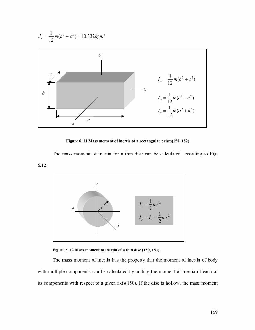
222 332.10)(121 kgmcbmJ c =+=

y

c )(

121 22 cbmI x +=

xb

)(121 22 acmI y +=

)(121 22 bamI z +=

a z

Figure 6. 11 Mass moment of inertia of a rectangular prism(150, 152)

The mass moment of inertia for a thin disc can be calculated according to Fig.

6.12.

y

2

21 mrI x = z r

2

21 mrII zy ==

x

Figure 6. 12 Mass moment of inertia of a thin disc (150, 152)

The mass moment of inertia has the property that the moment of inertia of body

with multiple components can be calculated by adding the moment of inertia of each of

its components with respect to a given axis(150). If the disc is hollow, the mass moment

159

of inertia is calculated by subtracting the outer diameter from the inner diameter as

follows:

)(21 22

ie rrmI −= (6.3.18)

where : is the exterior radius of the disc, : is the interior radius of the disc. er ir

To calculate the moment of inertia of Bearcat Cub wheel Eq. (6.3.18) can be

used, however, the wheel consists of two components a rubber tire and a plastic disc as

shown in Fig. 6.13. The exterior radius re=0.228m, the interior radius ri =0.190m, width

of the tire is 0.076m, the width of the plastic disc 0.0508m, the density of plastic disc is

1g/cc, the density of the rubber tire is 1.5g/cc(153), so the mass of the rubber tire and the

mass of the plastic disc can be calculated as mt=5.73kg, mr=5.67kg, respectively. The

total mass of the wheel is 11.4kg.

wJ

The moment of inertia for the robot wheel is calculated as:

2222 148.021)(

21 kgmrmrrmJ tirtitetw =+−= (6.3.19)

In , substituting the value of Jw from Eq. (6.3.19) and mw = 11.4 kg for

Bearcat Cub, J0 = 0.74kgm

20 rmJJ ww +=

2 is obtained,

Figure 6. 13 Segway tire structure (154)

160

Calculation of the resultant normal force fn

There are two main components in fn as shown in Fig. 6.8 (c). One is the reaction

to the normal friction force between the wheel and the ground; another is the centrifugal

force which represents the tendency of the wheel to leave its curved path.

fn can be calculated as follows:

cn fNf += µ (6.3.20)

where µ is the friction coefficient between the ground and the wheel; N is the normal

force between the wheel and the ground; fc is the centrifugal force.

The normal force N is the reaction to the gravitational forces that is also two

components (as shown in Fig. 6.8 (b).). One component is the weight of the wheel and

another is the portion of the weight of the robot that is carried by the wheel. Bearcat Cub

has three wheels and it is assumed that the weight of the robot is equally distributed on

the three wheels. Hence, N can be calculated as follows:

gmPN w+= (6.3.21)

mgP31

=

where mw: is the total mass of the wheel, and m is the mass of the robot excluding the

wheels.

The centrifugal force fc can be calculated as follows(150):

ρυ 2mfc = (6.3.22)

where v: is the velocity of the robot in the direction toward the center of the circular path.

ρ: is the radius of the circular path. v the velocity of the robot toward the center of the

161

circular path (IC as shown in Fig.6.8 (a)) is very small, and radius of the circular path ρ is

very large, therefore, the centrifugal force fc is very small and can be neglected.

Hence, the resultant normal force fn is only attributed to the reaction to the normal

force as follow:

)31( gmmgf wn += µ (6.3.23)

The value of the frictional coefficient µ between the ground and the wheel

depends on the type of the surface of the ground. µ=0.6 for grass in the calculations is

used since Bearcat Cub usually moves on grass. Substituting the parameters for Bearcat

Cub into equation (6.2.23), the following value is given:

fn = 356.56 N

Substituting the values of m, r, e, d, J0, Jc and fn into Eq. (6.3.17), Bearcat Cub

dynamic model is:

τζζζζζζζζ =++ ),,(),()( &&&&&&& GJM (6.3.24)

where:

⎥⎥⎥

⎦

⎤

⎢⎢⎢

⎣

⎡=

θζ c

c

yx

⎥⎦

⎤⎢⎣

⎡=

l

r

ττ

τ

⎥⎦

⎤⎢⎣

⎡

−−+−

=21.4cossin15.5sin15.5sin20cos2021.4cossin15.5sin15.5sin20cos20

)( 2

2


ζM

⎥⎦

⎤⎢⎣

⎡

+−−+−−

=)cos(sincos15.5cos24.3sin24.3)cos(sincos15.5cos24.3sin24.3

),(θθθθθθθθθθθθθθθθ

ζζ&&&

&&&&J

⎥⎦

⎤⎢⎣

⎡

−−−−−−

=60cossin6cossin660cossin6cossin6

),,(2222

2222

θθθθθθθθθθθθθθ

ζζζ&&&&

&&&&&&&G

6.4 Computed Torques Using MathCad and MatLab

6.4.1 Dynamic model verification using MathCad

162

The Bearcat Cub robot parameters are listed in the following:

mb 147.72:= r 0.2286:= Jo 0.74:= Jc 10.332:= d 0.4191:= es 0.3084:= fn 356.56:=

The following robot path is selected:

θ t( )π sin t( )

2:= 6.4.1( ) x t( ) sin t( ):= y t( ) cos t( ):=

The first derivatives of position are given, which expressed as the robot velocity with respect to the gravity center of the robot:

tθ t( )d

d12

π cos t( )⋅⋅→ tx t( )d

dcos t( )→

ty t( )d

dsin t( )−→ (6.4.2)

2t

x t( )d

d

2sin t( )−→

2ty t( )d

d

2cos t( )−→

2tθ t( )d

d

2 1−

2π sin t( )⋅⋅→ (6.4.3)

The second derivatives of robot position as the robot acceleration with respect to the gravity center of the robot:

The robot position, speed and acceleration are rewritten in the following as variables of the dynamic model:

ξ

x t( )

y t( )

θ t( )

⎛⎜⎜⎝

⎞

⎠

(6.4.4)

ξ t( )

sin t( )

cos t( )

π sin t( )2

⎛⎜⎜⎜⎜⎝

⎞⎟⎟

⎠

:= (6.4.5)

tξ t( )d

d

cost

sin t( )−

πcos t( )

2⋅

⎛⎜⎜⎜⎜⎝

⎞⎟⎟⎠

(6.4.6)

163

2tξ t( )d

d

2sin t( )−

cos t( )−

1− π sin t( )2

⎛⎜⎜⎜⎜⎝

⎞⎟⎟

⎠

(6.4.7)

According to the WMR dynamic model Eq. (6.3.17), we can calculate each component in the dynamic equation in order to obtain the total torques of the robot motion controller :

1. M (mass) component:

According to the dynamic model Eq. (6.3.16), we compute the elements of M component as the following:

M11mb r2⋅ cos θ t( )( )⋅( ) 2 Jo⋅ cos θ t( )( )⋅( )+⎡⎣ ⎤⎦

2 r⋅ (6.4.8)

M11 20 cos12

π sin t( )⋅⋅⎛⎜⎝

⎞⎠

⋅

M12mb r2⋅ sin θ t( )( )⋅( ) 2 Jo⋅ sin θ t( )( )⋅( )+⎡⎣ ⎤⎦

2 r⋅ (6.4.9)

M12 20 sin12

π sin t( )⋅⋅⎛⎜⎝

⎞⎠

⋅

M13mb r2⋅ es⋅ d⋅ sin θ t( )( )( )2

⋅⎡⎣ ⎤⎦ mb r2⋅ es⋅ d⋅ sin θ t( )( )⋅ cos θ t( )( )⋅( )− Jc r2⋅+ 2 Jo⋅ d2⋅+⎡⎣ ⎤⎦

2 r⋅ d⋅

(6.4.10)

M13 5.2 sin12

π sin t( )⋅⋅⎛⎜⎝

⎞⎠

2⋅ 5.2 sin

12

π sin t( )⋅⋅⎛⎜⎝

⎞⎠

cos12

π sin t( )⋅⋅⎛⎜⎝

⎞⎠

⋅⋅− 4.17+

164

(6.4.11) M21 M11

M22 M12

M23mb r2⋅ es⋅ d⋅ sin θ t( )( )2

⋅( ) mb r2⋅ es⋅ d⋅ sin θ t( )( )⋅ cos θ t( )( )⋅( )−⎡⎣ ⎤⎦ Jc r2⋅− 2 Jo⋅ d2⋅−

2 r⋅ d⋅

M23 5.2 sin12

π sin t( )⋅⋅⎛⎜⎝

⎞⎠

2⋅ 5.2 sin

12

π sin t( )⋅⋅⎛⎜⎝

⎞⎠

cos12

π sin t( )⋅⋅⎛⎜⎝

⎞⎠

⋅⋅− 4.17−

(6.4.12)

MM11

M21

M12

M22

M13

M23

⎛⎜⎜⎝

⎞

⎠ (6.4.13)

Now we calculate the torques TM1 and TM2 from M (mass) component:

(6.4.14) TMTM1

TM2⎛⎜⎝

⎞⎠

TM11 t( ) 20 cos12

π sin t( )⋅⋅⎛⎜⎝

⎞⎠

⋅ 2tx t( )d

d

2⎛⎜⎜⎝

⎞

⎠⋅:= (6.4.15)

TM12 t( ) 20 sin12

π sin t( )⋅⋅⎛⎜⎝

⎞⎠

⋅⎛⎜⎝

⎞⎠ 2t

y t( )d

d

2⎛⎜⎜⎝

⎞

⎠⋅:= (6.4.16)

TM13 t( ) 5.2 sin12

π sin t( )⋅⋅⎛⎜⎝

⎞⎠

2⋅ 5.2 sin

12

π sin t( )⋅⋅⎛⎜⎝

⎞⎠

cos12

π sin t( )⋅⋅⎛⎜⎝

⎞⎠

⋅⋅− 4.17+⎛⎜⎝

⎞

⎠ 2tθ t( )d

d

2⎛⎜⎜⎝

⎞

⎠⋅:=

(6.4.17)

TM1 t( ) TM11 t( ) TM12 t( )+ TM13 t( )+:= (6.4.18)

(6.4.19) TM21 t( ) TM11 t( ):=

(6.4.20) TM22 t( ) TM12 t( ):=

165

TM23 t( ) 5.2 sin12

π sin t( )⋅⋅⎛⎜⎝

⎞⎠

2⋅ 5.2 sin

12

π sin t( )⋅⋅⎛⎜⎝

⎞⎠

cos12

π sin t( )⋅⋅⎛⎜⎝

⎞⎠

⋅⋅− 4.17−⎛⎜⎝

⎞

⎠ 2tθ t( )d

d

2⎛⎜⎜⎝

⎞

⎠⋅:=

(6.4.21)

TM2 t( ) TM21 t( ) TM22 t( )+ TM23 t( )+:= (6.4.22)

2. J (Friction and other forces) component:

In the following, we compute the torques generated by friction and other forces except gravity:

J11 1.62− π cos t( ) sin12

π sin t( )⋅⋅⎛⎜⎝

⎞⎠

⋅⋅⋅ (6.4.23)

J12 1.62 π cos t( ) cos12

π sin t( )⋅⋅⎛⎜⎝

⎞⎠

⋅⋅⋅ (6.4.24)

J13 2.6− π cos t( ) cos12

π sin t( )⋅⋅⎛⎜⎝

⎞⎠

sin12

π sin t( )⋅⋅⎛⎜⎝

⎞⎠

cos12

π sin t( )⋅⋅⎛⎜⎝

⎞⎠

+⎛⎜⎝

⎞⎠

⋅⋅⋅⋅ (6.4.25)

J21 J11 J22 J12

J23 J13 (6.4.26)

Here TJ1(t) and TJ2(t) are the torques from J component

(6.4.27) TJTJ1

TJ2⎛⎜⎝

⎞⎠

166

(6.4.28) TJ11 t( ) 1.62− π cos t( ) sin12

π sin t( )⋅⋅⎛⎜⎝

⎞⎠

⋅⋅⋅⎛⎜⎝

⎞⎠ t

x t( )dd

⎛⎜⎝

⎞⎠

⋅:=

TJ12 t( ) 1.62 π cos t( ) cos12

π sin t( )⋅⋅⎛⎜⎝

⎞⎠

⋅⋅⋅⎛⎜⎝

⎞⎠ t

y t( )dd

⎛⎜⎝

⎞⎠

⋅:= (6.4.29)

T J13 t( ) 2.6 π cos t( ) cos12

π sin t( )⋅⋅⎛⎜⎝

⎞⎠

sin12

π sin t( )⋅⋅⎛⎜⎝

⎞⎠

cos12

π sin t( )⋅⋅⎛⎜⎝

⎞⎠

+⎛⎜⎝

⎞⎠

⋅⋅⋅⋅⎡⎢⎣

⎤⎥⎦

−tθ t( )d

d⎛⎜⎝

⎞⎠

⋅:=

(6.4.30)

(6.4.31) TJ1 t( ) TJ11 t( ) TJ12 t( )+ TJ13 t( )+:=

(6.4.32) TJ2 t( ) TJ11 t( ) TJ12 t( )+ TJ13 t( )+:=

3. G (Gravity) component:

Now we calculate the last component in the dynamic model, which is the torques produced by gravity:

G1=G2 TG1=TG2

(6.4.33)

G2 6tθ t( )d

d⎛⎜⎝

⎞⎠

2⋅ sin θ t( )( )( )2

⋅⎡⎢⎣

⎤⎥⎦ t

θ t( )dd

⎛⎜⎝

⎞⎠

2cos θ t( )( )( )2⎡

⎢⎣

⎤⎥⎦

− 6 2tθ t( )d

d

2⎛⎜⎜⎝

⎞

⎠⋅ sin θ t( )( )⋅ cos θ t( )( )⋅

⎡⎢⎢⎣

⎤⎥⎥⎦

− 60−

(6.4.33)

TG2 t( ) 6tθ t( )d

d⎛⎜⎝

⎞⎠

2⋅ sin θ t( )( )( )2

⋅⎡⎢⎣

⎤⎥⎦ t

θ t( )dd

⎛⎜⎝

⎞⎠

2cos θ t( )( )( )2⎡

⎢⎣

⎤⎥⎦

− 6 2tθ t( )d

d

2⎛⎜⎜⎝

⎞

⎠⋅ sin θ t( )( )⋅ cos θ t( )( )⋅

⎡⎢⎢⎣

⎤⎥⎥⎦

− 60−:=

(6.4.33)

167

4. Total torques Now we can get the total torques of the robot motion controller:

Tau1 t( ) TM1 t( ) TJ1 t( )+ TG1 t( )+:=(6.4.34)

Tau2 t( ) TM2 t( ) TJ2 t( )+ TG2 t( )+:=

We calculated each component of the dynamic model in Eq.(6.3.17). The equations verified that we got the correct computation in Eq. (6.3.24). The following are the graphs for the position and torques we obtained above.

t 0 0.1, 10..:=

0 2 4 6 8 102

0

2robot position

x t( )

y t( )

θ t( )

tFigure 6. 14 Robot position vectors

168

0 2 4 6 8 1040

20

0

20

40M component

TM1 t( )

TM2 t( )

t

Figure 6. 15 The torques by mass component

0 2 4 6 8 1020

15

10

5

0

5

10J component

TJ1 t( )

TJ2 t( )

t

Figure 6. 16 The torques by J component

169

0 2 4 6 8 1065

60

55

50G component

TG1 t( )

TG2 t( )

t

Figure 6. 17 The torques by G (gravity) component

0 2 4 6 8 10100

80

60

40

20

0Tau1, Tau2

Tau1 t( )

Tau2 t( )

t

Figure 6. 18 The total torques of the robot motion controller

170

6.4.2 Computed torques using Matlab

We used MatLab to compute the torques the same way as we did with MathCad

in previous section. The results are shown in the following figures (Fig. 6.19 – Fig. 6.23).

Comparing the computed torques using both MathCad and MatLab by using the same

robot trajectory as shown in Fig.19, all the graphs are matched with each other. It is clear

that the plot for the total computed torques Tau1 and Tau2, the mass component Tau1_M

and Tau2_M, J component Tau1_J and Tau2_J and the gravity component Tau1_G and

Tau2_G graphs are the same by using both MathCad and MatLab.

Figure 6. 19 Robot trajectory

171

Figure 6. 20 Computed torques – mass component

Figure 6. 21 Computed component- J component (friction forces related)

172

Figure 6. 22 Computed torques – gravity component

Figure 6. 23 Computed torques Tau1 and Tau2

173

6.5 Summary


mobile robots, which is a part of our current research projects. The scenarios for the

wheeled mobile robot- Bearcat Cub is developed according to the IGVC contest. Bearcat

Cub robot is designed for this challenge, moreover, it can be extended for the applications

such as mining, forest, agriculture, military, firefight, construction and other hazard fields

in unstructured environments.

The kinematics and dynamics analysis are two most important characteristics for

the mobile robot. By analyzing the position and velocity of the wheeled mobile robot

(WMR), the kinematic model of Bearcat Cub is obtained. In deriving the dynamic model

of the robot, the Newton-Euler method was used for dynamic analysis. It is noticed that

the dynamic model of the WMR is similar as the robot arm manipulator as used in the

arm simulation in Chapter 5. Bearcat Cub is one type of mobile robots with two fixed

wheels and one castor wheel. The Bearcat Cub dynamic model derived here is used for

simulation of the robot motion controllers in the next chapter.

In order to further analyze and verify the Bearcat Cub dynamic model, the torques

of each component in dynamic equation are computed by using both MathCad and

MatLab software. The plots of each component by MathCAD match the ones by Matlab.

The graphs of the total computed torques matches with each other as well.

174

CHAPTER 7 CASE STUDIES-WHEELED MOBILE

ROBOTS

The Bearcat Cub robot is a Wheeled Mobile Robots (WMR) as discussed in

Chapter 6. The navigation of WMR can be considered as the tracking problems. Alhaj

Ali’s (150) simulation framework on two-link robot manipulators is used to solve Bearcat

Cub robot (WMR)’s control problems. The simulation of the Bearcat Cub is similar to the

ones of the two-link robot arm manipulators by using different control methods such as

PD control, PID control, digital control and adaptive control. The purpose of the

simulation is to explore the control methods for the WMR Bearcat Cub and verify the

dynamic model of the robot developed in previous chapter.

The simulation results of Bearcat Cub robot are presented in this chapter. Section

7.1 is a brief description on the simulation architecture for the WMR motion controller.

The PD CT controller, PID CT controller, and digital CT controller are simulated in

Section 7.2, 7.3, 7.4 respectively. Section 7.5 addresses adaptive controller. In Section

7.6, an optimal PID controller is developed. The chapter is summarized in Section 7.7.

7.1 Simulation Architecture for WMR (Bearcat Cub)

The dynamics of the WMR robot equation (6.3.13) can be rewritten as:

τ=++ FqqqJqqM &&&& ),()( (7.1.1)

where M, J, F and τ were previously defined in equation (6.3.13) or (6.3.17) by replacing

ξ with q. The similarities between equation (7.1.1) and (5.1.1) make it possible to develop

a CT controller suitable for both two-link robot arm manipulator and WMR.

Now reformulate equation (7.1.1) as:

175

τ=+ ),()( qqNqqM &&& (7.1.2)

or, in the case of the existence of unknown disturbances τd:

ττ =++ dqqNqqM ),()( &&& (7.1.3)

where represents the nonlinear terms. ),( qqN &

The objective of a motion controller is to move the robot along the desired motion

trajectory qd(t). The actual motion trajectory is defined as q(t). The tracking error can be

defined as(11):

)()()( tqtqte d −= (7.1.4)

The Brunovsky canonical form can be developed by differentiating e(t) twice and writing

it in the terms of the state x (11):

uIe

eIee

dtd

⎥⎦

⎤⎢⎣

⎡+⎥

⎦

⎤⎢⎣

⎡⎥⎦

⎤⎢⎣

⎡=⎥

⎦

⎤⎢⎣

⎡ 000

0&& (7.1.5)

where:

)),()((1 τ−+≡ − qqNqMqu d &&&

⎥⎦

⎤⎢⎣

⎡= T

T

ee

x&

Then the torques needed for the motors are computed by using the inverse of the dynamic

equation for the WMR as shown in Eq.(6.3.16).

),())(( qqNuqqM d &&& +−=τ (7.1.6)

The simulation architecture for WMR is very similar to the one for the two-link

robot arm manipulator introduced in Chapter 5. The simulation program computes the

torques of the controller and then calculates the error dynamics of WMR navigation. The

program includes the following main components:

176

2. The first module computes the desired WMR trajectory qd(t) from the input of the

robot navigation system, such that,

⎥⎥⎥

⎦

⎤

⎢⎢⎢

⎣

⎡=

θd

d

d yx

q (7.1.7)

where: xc is the x-axis component of the desired position in terms of the WMR center of

gravity; yc: is the y-axis component of the desired position of the WMR center of gravity;

θ: is the desired orientation of the WMR.

2. The second module calculates the controller input from the tracking error between

the desired trajectory qd(t) and the actual trajectory q(t). The actual trajectory q(t)

is:

⎥⎥⎥

⎦

⎤

⎢⎢⎢

⎣

⎡=

θyx

q (7.1.8)

where: x: is the x-axis component of the actual position in terms of the WMR center of

gravity; y: is the y-axis component of the actual position in terms of the WMR center of

gravity; θ: is the actual orientation of the WMR. Then the inertia term M(q) and the

nonlinear term are computed by the WMR dynamic model described in Eq.

(7.1.1). Finally, the motion control torques is calculated by using Eq. (7.1.6).

),( qqN &

3. The third module calculates the new position of the WMR by using the state-space

equation, , where the state-space position/velocity form is used (11): ),( uxfx =&

⎥⎦

⎤⎢⎣

⎡≡ T

T

qq

x& (7.1.9)

177

τ⎥⎦

⎤⎢⎣

⎡+⎥

⎦

⎤⎢⎣

⎡−

= −− )(0

),()( 11 qMqqNqMq

x&

&&

(7.1.10)

This equation is used to update the WMR actual position.

7.2 PD CT Controller for WMR (Bearcat Cub)

7.2.1 PD CT controller

The Bearcat Cub WMR simulation program structure is similar to the one for the

two-link robot arm manipulator. It has three main modules as described in the previous

section. The inputs to the PD CT controller simulation program are:

• Desired motion trajectory qd(t);

, where c1, c2, c3 are constant ⎥⎥⎥

⎦

⎤

⎢⎢⎢

⎣

⎡

⋅⋅⋅

=⎥⎥⎥

⎦

⎤

⎢⎢⎢

⎣

⎡=

tctctc

yx

q

d

d

d

d

sincossin

3

2

1

θ

• Bearcat Cub robot parameters;

• Controller gain parameters kp and kv.

The outputs of the PD CT controller simulation program are:

• Motor torques τ(t);

• Actual path q(t).

• Robot parameters of Bearcat Cub are listed in Table 7.1.

7.2.2 Simulation results

The simulation is conducted in two cases and the gain matrices are carefully

chosen since the dynamics of the Bearcat Cub WMR is very complicated. A trial-and-

error method is used to achieve optimal simulation results.

178

Bearcat Cub parameters

m 147.72 kg

r 0.2286 m

0J 0.74kgm2

cJ 10.332 kgm2

e 0.3048m

d 0.4191m

nf 356.56 N

Table 7. 1 Bearcat Cub robot parameters.

Case I: Gain parameters for x, y and θ are equal

In the first set of experiments, the same kp and kv values are used for the three

components of the motion trajectory q(x, y, θ) and the results are:

1. Starting with kp=kv=0, the tracking errors are ranged from 0-0.3 as shown in Fig.

7.1. The desired versus actual trajectory is shown in Fig. 7.2. As it is shown in the

figures, the tracking errors are very high and the motion trajectories are unstable.

179

Figure 7. 1 Tracking errors for WMR with a PD CT controller, kp=kv=0: Unstable.

Figure 7. 2 Desired and actual trajectories for WMR with a PD CT controller, kp=kv=0.

3. After increasing with kp= 2, and kv=1, the tracking errors for x and θ are

converged to 0 at time 10sec as shown in Fig. 7.3. It is shown in Fig. 7.4 that the

actual path and desired path matched for x and θ at time 10sec. There is some

improvement on y direction’s performance.

Figure 7. 3 Tracking errors for WMR with a PD CT controller, , kp=2, kv=1: Unstable.

Figure 7. 4 Desired and actual trajectories for WMR with a PD CT controller, , kp=2, kv=1.

3. After increasing kp= 10, and kv= 1, the tracking errors and the desired and actual

trajectory are shown in Figs. 7.5, 7.6. It is shown that it’s faster for x and θ to

converge to 0. Otherwise, there is not much improvement for y- oscillation about

zero.

180


Figure 7. 6 Desired and actual trajectories for WMR with a PD CT controller, kp=10, kv=1.

4. Increasing the value of kp to 20 and the value of kv to 10, the performance of the

controller is shown in Figs. 7.7, 7.8. It is the best result obtained so far. The

tracking errors for x and θ are converged to 0 at less than 2 seconds. However,

there is not much improvement for y.

Figure 7. 7 Tracking errors for WMR with a PD CT controller, kp=20, kv=10.: Unstable.


181

5. Increasing the value of kp to 100 and the value of kv to 10, the simulation results

are shown in Fig. 7.9, 7.10. The tracking errors for x and θ are as good as the

previous simulation results with kp =20, and kv = 10. The performance for y still

remains the same.



Case II: Controller gain parameters for x, y and θ are different

1. Starting with kp1=2, kv1=1, kp2=0, kv2=10, kp3=2, and kv3=1, the simulation

results are shown in Figs.7.11, 7.12. The tracking errors for x and θ are converged

to 0 at time 10sec as shown in Fig. 7.11. It is shown in Fig. 7.12 that the actual

path and desired path matched for x and θ at time 10sec. There is some

improvement on y direction’s performance. The performance is almost the same

as in Case I when using equal gain parameters kp=2, kv=1. It implies that

changing kp2=0, kv2=10 doesn’t affect the performance of x, θ.

182

Figure 7. 11 Tracking errors for WMR with a PD CT controller, kp1=2, kv1=1, kp2=0, kv2=10, kp3=2, and kv3=1. Unstable.

Figure 7. 12 Desired and actual trajectories for WMR with a PD CT controller, kp1=2, kv1=1, kp2=0, kv2=10, kp3=2, and kv3=1.

2. Using kp1=15, kv1=7, kp2=20, kv2=100, kp3=100, and kv3=50, the tracking errors

and desired and actual motion trajectories are shown in Figs. 7.13, 7.14,

respectively. It gave us a good performance except that the tracking error for y

still stays the same- oscillation about zero.



183

3. Keeping kp1=15, kv1=7, changing kp2=10, kv2=5, and increasing kp3=2000, and

kv3=1000, the results of the simulation are shown in Figs. 7.15 and 7.16. These

results are observed to be better than those in the previous two experiments.



4. Increasing kp1=1000, kv1=400, kp2=200, kv2=100 and keeping kp3=2000, and

kv3=1000, the results of the simulation are shown in Figs. 7.17 and 7.18. These

results are almost the same as the previous experiment. The increase of kp1=1000,

kv1=400, kp2=200, kv2=100 doesn’t change the motion trajectory of x, y and θ.

184



7.2.3 Conclusions

As shown in the above figures, selection of the gain parameters is critical to a

good performance of the controller. According to the trial-and-error methods, the

simulation results are summarized as the following:

• Better results are obtained for x, and θ by increasing the value of kp1, kv1, kp3, and kv3

no matter the values of the parameters are the same or different.

• Simultaneously, it sounds that the value of kp1 should set as double of kv1 in order to

achieve better results.

• It is noticed that the values of parameters kp2, and kv2 should not be too large, but it

seems very difficult to select a good set of parameters kp2, and kv2 to obtain the

desired motion trajectory in y direction.

The simulation results above show that changing the gain matrices can obtain better

performance but these changes could be arbitrary if there is no optimal method to do so.

An optimization simulation in obtaining the gain matrices is recommended.

185

7.3 PID CT Controller for WMR (Bearcat Cub)

7.3.1 PID CT controller

The Bearcat Cub WMR simulation program is similar to the one for PD CT

controller in previous section. In PID CT controller, a integral component ki is added in

the PD CT controller. The inputs to the PID CT controller simulation program are:



• PID controller parameters kp, kv, and ki.

The outputs of the PID CT controller simulation program are:


• Actual path q(t).

Bearcat Cub robot parameters are listed in Table 7.1. The simulation is conducted

using two different desired motion trajectories.


The results are summarized in the following.

Case I: Using a sinusoidal desired motion trajectory:

⎥⎥⎥

⎦

⎤

⎢⎢⎢

⎣

⎡

⋅⋅⋅

=⎥⎥⎥

⎦

⎤

⎢⎢⎢

⎣

⎡=

tctctc

yx

q

d

d

d

d

sincossin

3

2

1

θ (7.3.1)

where c1, c2, c3 is constant (150).

1. Starting with small positive values for kp, kv and ki, where kp=1, kv=1 and ki =1,

the tracking errors increase as the simulation goes on and the control system is not

186

stable as shown in Fig. 7.19. The desired versus the actual motion trajectories are

shown in Fig. 7.20. It is obvious that the simulation results, the tracking errors did

not converge to zero so this set of parameters is not acceptable and the controller

is unstable.

Figure 7. 19 Tracking errors for WMR with a PID CT controller, kp=1, kv=1, ki=1. (sin) Unstable.

Figure 7. 20 Desired and actual trajectories for WMR with a PID CT controller, , kp=1, kv=1, ki=1. (sin)

2. In the second of parameters, increasing the values of kp, and k, let kp=2, kv=3 and

keep ki =1, the simulation results for the tracking errors and desired versus actual

motion trajectory are shown in Figs 7.21, 7.22, respectively. The tracking errors x,

y are oscillated around zero but tracking error of θ is converged to zero. The

simulation performance improved comparing to the first set of data.

187


Figure 7. 22 Desired and actual trajectories for WMR with PID controller, kp=2, kv=3, ki=1. (sin)

3. In the third experiment, increasing the values of ki to 2 and keep kp=2, kv=3, the

simulation results for the tracking errors and desired versus actual motion

trajectory are shown in Figs 7.23, 7.24, respectively. The tracking error of θ is

converged to zero but the tracking errors x, y are oscillated and unstable. Thus,

increasing ki to 2 is not a good option.

Figure 7. 23 Tracking errors for WMR with a PID CT controller, kp=2, kv=3, ki=2 (sin). Unstable.

Figure 7. 24 Desired and actual trajectories for WMR with a PID CT controller, , kp=2, kv=3, ki=2 (sin).

188

4. In the forth trial, let kp=2, kv=20 and ki=1. The simulation result is shown in Figs

7.25, 7.26. The tracking errors are ranged from -0.6 -0.6 shown in Fig. 7.25.

None of the tracking errors converged so the controller is not stable. Therefore,

increasing kv to 20 is not a good option.


Figure 7. 26 Desired and actual trajectories for WMR with a PID CT controller, kp=2, kv=20, ki=1 (sin).

5. In the fifth set of experiment, let kp=10, kv=3 and ki=1. The tracking errors are

shown in Fig. 7.27 and the desired versus actual trajectories are shown in Fig.

7.28. Comparing the result with the set of data [kp=2, kv=3 and ki=1], the

tracking error of θ converged to zero faster but the tracking errors of x, y

increased and are not stable. Therefore, only increasing kp to 10 is not a good

option.

189


Figure 7. 28 Desired and actual trajectories for WMR with a PID CT controller, kp=10, kv=3, ki=1 (sin).


⎥⎥⎥

⎦

⎤

⎢⎢⎢

⎣

⎡

⋅⋅+⋅

⋅=

⎥⎥⎥

⎦

⎤

⎢⎢⎢

⎣

⎡=

tctctc

tcyx

q

d

cd

cd

d

sin3

22

1

21

θ (7.3.2)

where c1,c2, and c3 are constants(150).

1. Starting with the set of values [kp=1, kv=1 and ki =1], the tracking errors increase

as the simulation goes on and the control system is not stable as shown in Fig. 7.29.

The desired versus the actual motion trajectories are shown in Fig. 7.30. The

tracking errors did not converge to zero and the controller is not stable. Thus, this

set of parameters is not acceptable.

190

Figure 7. 29 Tracking errors for WMR with a PID CT controller, kp=1, kv=1, ki=1. Unstable.

Figure 7. 30 Desired and actual trajectories for WMR with a PID CT controller, kp=1, kv=1, ki=1..

2. In the second of parameters, increasing the values of kp, and k, let kp=2, kv=3 and

keep ki =1, that is, K=[ kp=2, kv=3, ki =1], the simulation results for the tracking

errors and desired versus actual motion trajectory are shown in Figs 7.31, 7.32,

respectively. The tracking errors of x, y θ are converged to zero at 20 second

moment of time. The desired trajectory and the actual motion trajectory match each

other after 20 second of simulation. The simulation performance obtained the best

results so far. It is an acceptable set of experiment data.

Figure 7. 31 Tracking errors for WMR with a PID CT Figure 7. 32 Desired and actual trajectories for WMR

191

controller, kp=2, kv=3, ki=1. Stable with a PID CT controller, kp=2, kv=3, ki=1..

3. In the third set of experimental parameters, increasing ki to 5, that is, let K=[ kp=2,

kv=3, ki =5], the simulation results for the tracking errors and desired versus actual

motion trajectory are shown in Figs 7.33, 7.34, respectively. Comparing to the

previous experiment, changing ki to 5 is a disaster for the controller. The control

system became unstable.



4. In the fourth set of parameters, increasing kv to 20, that is, let K=[ kp=2, kv=20, ki

=1], the simulation results for the tracking errors and desired versus actual motion

trajectory are shown in Figs 7.35, 7.36, respectively. Comparing to the previous

experiment set [ kp=2, kv=3, ki =1], changing kv to 20 is not a good choice on the

gain matrices of the controller. The performance of the controller did not improve

by increasing kv to 20.

192



5. In the fifth set of parameters, increasing kp to 5, that is, let K= [ kp=5, kv=3, ki =1],

the simulation results for the tracking errors and desired versus actual motion

trajectory are shown in Figs 7.37, 7.38, respectively. The tracking error of θ is

converged to zero but it’s a disaster for x, y. The performance of the controller did

not improve by only changing kp to 5.



193

7.3.3 Conclusions

As shown in the simulation results above, it is clear that the values of kp, kv, and ki

need to be small positive numbers to obtain good results. It is obvious that using very

high, or zeros, values for kp, kv, and ki is not recommended. The integral controller ki can

not be too large the tracking error stable. Each of gain matrices Kp, Kv, and Ki on a

closed-loop system are dependent of each other. In fact, changing one of these variables

can change the effect of the other two. Thus, developing an optimal method on how to

select the gain matrices is recommended.

When choosing K=[kp=2 kv=3 and ki=1] as a set of trial parameters, the

simulation results are acceptable. Therefore, using these values and adjusting them more

or less with a small value is recommended.

7.4 Digital CT Controller for WMR (Bearcat Cub)

7.4.1 Digital controller for WMR

The control law for the WMR is the similar to two-link robot arm manipulator as

described in Eq. (5.4.1). The digital controller simulation program for Bearcat Cub WMR

is developed by using the WMR dynamics derived in the previous chapter. The Bearcat

Cub WMR parameters are listed in table 7.1.

The inputs to the digital controller simulation program are:



• Controller parameters kp, kv.

The outputs of the digital controller simulation program are:

194


• Actual path q(t), and tracking errors.


The simulation is conducted by using two different desired motion trajectories.

The sample period T=20msec are used for all the cases. The results are summarized in the

following.

Case I: Using a sinusoidal desired motion trajectory(150):

⎥⎥⎥

⎦

⎤

⎢⎢⎢

⎣

⎡

⋅⋅⋅

=⎥⎥⎥

⎦

⎤

⎢⎢⎢

⎣

⎡=

ttt

yx

q

d

d

d

d

sin01.0cos01.0sin01.0

θ (7.4.1)

1. Let the controller gain matrix K: [kp =2, kv=1], the simulation results are shown in

Figs 7.39, 7.40. The tracking errors for x and θ are converged to zero but the

tracking error of y is off the center of zero as shown in Fig. 7.39. In Fig. 7.40, we

can see actual trajectories x and θ match their desired trajectories but not for y

direction.

Figure 7. 39 Tracking errors for WMR with a digital Figure 7. 40 Desired and actual trajectories for WMR

195

CT controller, kp=2, kv=1. (sin) Unstable. with a digital CT controller, kp=2, kv=1. (sin)

2. Now increasing the value of kv to 100, so the gain matrix K is [kp =2, kv=100], the

simulation results of the tracking errors and the desired and actual trajectories are

shown in Figs 7.41, 7.42. This change of kv to100 made the controller’s

performance worse. It’s not a set of parameters to be chosen for a controller.

Figure 7. 41 Tracking errors for WMR with a digital CT controller, kp=2, kv=100. (sin) Unstable.

Figure 7. 42 Desired and actual trajectories for WMR with a digital CT controller, kp=2, kv=100. (sin)

Case II: Using the following desired motion trajectories(150):

⎥⎥⎥

⎦

⎤

⎢⎢⎢

⎣

⎡

⋅+

⋅=

⎥⎥⎥

⎦

⎤

⎢⎢⎢

⎣

⎡=

ttt

tyx

q

d

d

d

d

sin001.0008.00005.0

0005.02

2

θ (7.4.2)

1. Let the controller gain matrix K: [kp =2, kv=1], the simulation results are shown in

Figs 7.43, 7.44. The tracking errors are ranged from -0.01 to 0.02. The tracking

errors for x and θ are converged to zero and the tracking error of y reduced to -

0.05 as shown in Fig. 7.43. In Fig. 7.44, it is clear that the actual trajectories x, y

196

and θ are very smooth and tend to match their desired trajectories. This set of

parameters is the best results obtained so far.


Figure 7. 44 Desired and actual trajectories for WMR with a digital CT controller, kp=2, kv=1

2. Now increasing the value of kv to 100, so let the gain matrix K: [kp =2, kv=100],

the simulation results of the tracking errors and the desired and actual trajectories

are shown in Figs 7.45, 7.46. It is clear that the tracking error of x is converged to

-0.01 instead of zero. It implies that when the gain kv is too big, it will increase the

steady state error.

197


Figure 7. 46 Desired and actual trajectories for WMR with a digital CT controller, kp=2, kv=100

3. Now increasing kp to 50, let the gain matrix K: [kp =50, kv=1], the simulation

results of the tracking errors and the desired and actual trajectories are shown in

Figs 7.47, 7.48. Comparing the simulation results by using set of [kp =2, kv=1],

the tracking errors is oscillated around zero and the control system is not settled.


Figure 7. 48 Desired and actual trajectories for WMR with a digital CT controller, , kp=50, kv=1

7.4.3 Conclusions

Increasing the value of kv does not improve the simulation results. However,

increasing the value of does as long as the value maintains in a certain range. When

choosing K=[kp=2 kv=1] as a set of trial parameters, better performance results are

achieved as shown in the simulation results. Therefore, using these values and adjusting

them more or less with a small value is recommended.

pk

198

Comparing the simulation performance of the three controllers discussed above,

namely, PD CT, PID CT, and the digital CT controller, it is observed that the PID CT

controller provides the best results. Therefore, it is recommended for this application.

7.5 Adaptive Controller for WMR (Bearcat Cub)

7.5.1 Adaptive controller architecture

The filtered-error approximation-based adaptive controller for WMR navigation is

developed from Eq. 6.2.12. The regression matrix W(x) can be derived from the WMR

dynamics presented in previous chapter. The regression matrix WR(x) for WMR needs to

be developed from error dynamics Eq. A.78-A.79 (11) and WMR dynamics(150):

ψ)())(,())(()( xWRFEqqqJEqqMxf dd =+Λ++Λ+= &&&&& (7.5.1)

ψ)()(ˆ xWRxf = (7.5.2)

where: [ ]TTd

Td

Td

TT qqqEEx &&&&=

))(( EqqM d&&& Λ+ , ) , are 2x1 matrices, so is a 2x1 matrix. The

regression matrix and the vector of the unknown robot parameters,

)(,( EqqqJ d Λ+&& F )(xf

ψ)(xWR , need to be a

2x1 matrix. There are many options for that. However, it is best to choose the to be

a 2x2 matrix and

)(xWR

ψ to be a 2x1 matrix. The unknown parameter is selected to contain

mass (11). Therefore, m ψ can be set as follows:

⎥⎦

⎤⎢⎣

⎡=

1ˆ

mψ (7.5.3)

The regression matrix can be written as(150):

199

⎥⎦

⎤⎢⎣

⎡=

2221

1211)(WRWRWRWR

xWR (7.5.4)

Now, the matrices must satisfy the following(150): ,,, 211211 WRWRWR 22WR

ψ)()( xWRxf = (7.5.5)

where:

FEqqqJEqqMxf dd +Λ++Λ+= ))(,())(()( &&&&&

⎥⎥⎥

⎦

⎤

⎢⎢⎢

⎣

⎡=

θe

c

yx

q

⎥⎥⎥⎥

⎦

⎤

⎢⎢⎢⎢

⎣

⎡

−−−++

++−++

=

rddJrJedmredmr

rJmr

rJmr

rddJrJedmredmr

rJmr

rJmr

qMc

c

2)2cossinsin(

2)sin2sin(

2)cos2cos(

2)2cossinsin(

2)sin2sin(

2)cos2cos(

)( 20

22220

20

2

20

22220

20

2

θθθθθθθ

θθθθθθθ

⎥⎥⎥⎥

⎦

⎤

⎢⎢⎢⎢

⎣

⎡

+−−

+−−

=

2)cos(sincoscossin

2)cos(sincoscossin

),(00

00

θθθθθθθθ

θθθθθθθθ

&&&

&&&

&mre

rJ

rJ

mrer

Jr

J

qqJ

⎥⎥⎥⎥

⎦

⎤

⎢⎢⎢⎢

⎣

⎡

−

−

=

derf

derf

Fn

n

The elements of matrix can be derived(150): 22211211 ,,, WRWRWRWR )(xWR

derf

Sr

JS

rJ

Srd

dJrJS

rJ

Sr

JWR

SreSrd

edredrSr

rSr

rWR

derf

Sr

JS

rJ

Srd

dJrJS

rJ

Sr

JWR

SreSrd

edredrSr

rSr

rWR

nc

nc

−+−+

−+=

+−

−++=

−+−+

++=

+−

−++=

20

10

3

20

2

20

10

22

33

222

2

2

1

2

21

20

10

3

20

2

20

10

12

33

222

2

2

1

2

11

cossin2

22sin2

2cos2

2)cos(sincos

2cossinsin

2sin

2cos

cossin2

22sin2

2cos2

2)cos(sincos

2cossinsin

2sin

2cos

θθθθθθ

θθθθθθθθθ

θθθθθθ

θθθθθθθθθ

&&&&&

&&&&

&&&&&

&&&&

(7.5.6)

Now, the regression matrix for the WMR can be expressed as(150):

200

⎥⎥⎥⎥

⎦

⎤

⎢⎢⎢⎢

⎣

⎡

−+−+

−++

−−

++

−+−+

+++

−−

++=

derfS

rJS

rJS

rddJrJS

rJS

rJSreS

rdedredrS

rrS

rr

derfS

rJS

rJS

rddJrJS

rJS

rJSreS

rdedredrS

rrS

rr

xWRnc

nc

20

10

3

20

2

20

10

33

222

2

2

1

2

20

10

3

20

2

20

10

33

222

2

2

1

2

cossin2

22sin2

2cos2

2)cos(sincos

2cossinsin

2sin

2cos

cossin2

22sin2

2cos2

2)cos(sincos

2cossinsin

2sin

2cos

)(θθθθθθθθθθθθθθθ

θθθθθθθθθθθθθθθ

&&&&&

&&&&

&&&&&

&&&&

(7.5.7)


Two sets of simulation are performed on WMR adaptive controller. In the first set,

a sinusoidal trajectory is used and a quadratic trajectory is used for the second set. In the

adaptive controller simulation, three critical matrices ,vK Λ , Γ need to be adjusted to

obtain optimal performance.

Case I: Using a sinusoidal desired motion trajectory:

⎥⎥⎥

⎦

⎤

⎢⎢⎢

⎣

⎡

⋅⋅⋅

=⎥⎥⎥

⎦

⎤

⎢⎢⎢

⎣

⎡=

ttt

yx

q

d

d

d

d

sin1.0cos1.0sin1.0

θ (7.5.8)

The simulation robot and controller parameters are listed in tables 7.1, 7.2, respectively.


vK ⎥⎦

⎤⎢⎣

⎡020002

Λ ⎥⎥⎥

⎦

⎤

⎢⎢⎢

⎣

⎡=

⎥⎥⎥

⎦

⎤

⎢⎢⎢

⎣

⎡

300030003

000000

3

2

1

λλ

λ

Γ ⎥⎦

⎤⎢⎣

⎡1000

0100

Table 7. 2 Adaptive controller simulation parameters for WMR.

201

The simulation results are shown in Figs. 7.49-7.51. The tracking errors are in the

range of -2.5 to 0.5 and are not converged to zero as shown in Fig. 7.49. The actual

motion trajectories and desired motion trajectories are not matched with each other as

shown in Fig. 7.50. However, the controller was able to approximate the unknown robot

parameters. The first unknown robot parameter (mass) increases from zero to around 320

kg, and the second unknown robot parameter (1) oscillates around one, which is its actual

value as shown in Fig.7.51.

Figure 7. 49 Adaptive controller tracking errors (2, 3, 100). Unstable.

Figure 7. 50 Adaptive controller desired versus actual motion trajectories. (2, 3, 100)

202

Figure 7. 51 Adaptive controller parameters estimate. (2, 3, 100)

Case II: The following desired motion trajectories are used:

⎥⎥⎥

⎦

⎤

⎢⎢⎢

⎣

⎡

+⋅

=⎥⎥⎥

⎦

⎤

⎢⎢⎢

⎣

⎡=

ttt

tyx

q

d

d

d

d

sin01.001.0

01.02

2

θ (7.5.9)

1. In the first experiment of this case, the following controller parameters are

used:


vK ⎥⎦

⎤⎢⎣

⎡020002

Λ

⎥⎥⎥

⎦

⎤

⎢⎢⎢

⎣

⎡=

⎥⎥⎥

⎦

⎤

⎢⎢⎢

⎣

⎡

300030003

000000

3

2

1

λλ

λ

Γ ⎥⎦

⎤⎢⎣

⎡150015


The results of the simulation are shown in Figs. 7.52-7.54. The integrator works

for three time units for this path. The tracking errors of the adaptive controller are

not converged to zero as shown in Fig. 7.52. It shows that the actual motion

trajectories match with the desired trajectories at first and then grow further apart

as shown in Fig.7.53. The controller is not able to approximate the unknown robot

203

parameters. The control system is not able to reach stable state. Note that the

integrator only runs 3 time units in this simulation.

Figure 7. 52 Adaptive controller tracking errors (2, 3, 15). Unstable.

Figure 7. 53 Adaptive controller desired versus actual motion trajectories.(2, 3, 15)

Figure 7. 54 Adaptive controller parameters estimate (2, 3, 15).

2. To study the effect of increasing, Γ , a second experiment in this set is performed

by using the same controller parameters as in case I :


204

vK ⎥⎦

⎤⎢⎣

⎡020002

Λ

⎥⎥⎥

⎦

⎤

⎢⎢⎢

⎣

⎡=

⎥⎥⎥

⎦

⎤

⎢⎢⎢

⎣

⎡

300030003

000000

3

2

1

λλ

λ

Γ ⎥⎦

⎤⎢⎣

⎡1000

0100


The results of the experiment are shown in Figs. 7.55-7.57. The integrator works

for 6 time units for this simulation. The controller can approximate the unknown

robot parameters, where the first unknown robot parameter (mass) increases from

zero to around 320 kg, while the second unknown robot parameter (1) oscillates

around one, which is its actual value as shown in Fig.7.57. This result is very

close to the result from case I. The tracking errors are in a range of -0.6 to 0.6 as

shown in Fig. 7.55. The tracking error pattern is different from case I even though

the same set of controller parameters are used in the simulation. At first, the actual

trajectories of x, y gradually follows the desired ones around 4 time units but then

go far apart from each other. The controller can not reach stable state.

205

Figure 7. 55 Adaptive controller tracking errors.

(2, 3 ,100) Unstable.


Figure 7. 57 Adaptive controller parameters estimate.

(2, 3, 100)

3. To study the effect of increasing, Γ , a second experiment in this set is performed

by changing to1000 as shown in the following table: Γ

vK ⎥⎦

⎤⎢⎣

⎡020002

206

Λ

⎥⎥⎥

⎦

⎤

⎢⎢⎢

⎣

⎡=

⎥⎥⎥

⎦

⎤

⎢⎢⎢

⎣

⎡

300030003

000000

3

2

1

λλ

λ

Γ ⎥⎦

⎤⎢⎣

⎡10000

01000

Table 7. 5 Adaptive controller simulation parameters for WMR navigation.

The results of the experiment are shown in Figs. 7.58-7.60. The controller can

approximate the unknown robot parameters, where the first unknown robot

parameter (mass) increases from zero to around 320 kg, while the second

unknown robot parameter (1) oscillates around one, which is its actual value as

shown in Fig.7.60. The tracking errors are in a range of -0.1 to 0.5 as shown in

Fig. 7.58. The actual trajectories grow apart from the desired ones before 5 time

units, but the actual trajectories gradually match the desired ones afterwards.

Figure 7. 58 Adaptive controller tracking errors.

(2, 3 ,1000) Unstable.


207

(2, 3, 1000) Figure 7. 60 Adaptive controller parameters

estimate.

4. To study the effect of parameters , another experiment in this case is

performed, with the following controller parameters:

vK


vK ⎥⎦

⎤⎢⎣

⎡050005

Λ

⎥⎥⎥

⎦

⎤

⎢⎢⎢

⎣

⎡=

⎥⎥⎥

⎦

⎤

⎢⎢⎢

⎣

⎡

300030003

000000

3

2

1

λλ

λ

Γ ⎥⎦

⎤⎢⎣

⎡1000

0100


The results of the experiment are shown in Figs. 7.61-7.63. Note that the

integrator only runs 3 time units in this simulation. The controller can not

approximate the unknown robot parameters as shown in Fig.7.63. The tracking

208

errors can not be converged as shown in Fig. 7.61. The actual trajectories grow

apart from the desired ones as shown in Fig. 7.62. Thus, increasing the gain

makes the controller performance worse.

vK

Figure 7. 61 Adaptive controller tracking errors. (5, 3 ,100) Unstable.



(5, 3, 100)

5. To study the effect of parameters Λ , another experiment in this case is performed,

with the following controller parameters:

209


vK ⎥⎦

⎤⎢⎣

⎡020002

Λ

⎥⎥⎥

⎦

⎤

⎢⎢⎢

⎣

⎡=

⎥⎥⎥

⎦

⎤

⎢⎢⎢

⎣

⎡

500050005

000000

3

2

1

λλ

λ

Γ ⎥⎦

⎤⎢⎣

⎡100010



integrator only runs 4 time units in this simulation. The controller can

approximate the unknown robot parameters as shown in Fig.7.66, where the first

unknown robot parameter (mass) increases from zero to around 320 kg, while the

second unknown robot parameter (1) oscillates around one and still need some

time to reach the desired value 1. The tracking errors are in range of -0.2 to 0.2

shown in Fig.7.64. The actual and desired trajectories can not match each other

but it is obvious that the tracking errors become smaller after 3.5 time units. The

controller is not in a stable state in 4 time units.

210




(2, 5, 10)

6. To study the effect of parameters Λ and Γ , another experiment in this case is

performed, with the following controller parameters:


vK ⎥⎦

⎤⎢⎣

⎡020002

211

Λ

⎥⎥⎥

⎦

⎤

⎢⎢⎢

⎣

⎡=

⎥⎥⎥

⎦

⎤

⎢⎢⎢

⎣

⎡

500050005

000000

3

2

1

λλ

λ

Γ ⎥⎦

⎤⎢⎣

⎡1000

0100



integrator only runs 4 time units in this simulation. The controller can

approximate the unknown robot parameters, where the first unknown robot

parameter (mass) increases from zero to around 300 kg, while the second

unknown robot parameter (1) oscillates around one, which is its actual value as

shown in Fig.7.69. The tracking errors are in range of -1 to 0.2 shown in Fig.7.67.

The actual and desired trajectories can not match each other. The results show that

the change of Γ can not improve the tracking errors but improve the performance

of estimating unknown robot parameters.

212




(2, 5, 100)

7.5.3 Conclusions

It’s important to consider the problems with the simulation software Matlab,

which can not conduct 10 time units for adaptive controller as it does with other CT

controllers above. According to the simulation results shown in the figures above, the

simulation parameters in the following are recommended to produce better performance.


vK ⎥⎦

⎤⎢⎣

⎡020002

Λ

⎥⎥⎥

⎦

⎤

⎢⎢⎢

⎣

⎡=

⎥⎥⎥

⎦

⎤

⎢⎢⎢

⎣

⎡

500050005

000000

3

2

1

λλ

λ

Γ ⎥⎦

⎤⎢⎣

⎡100010

213

Table 7. 9 Recommended adaptive controller parameters for WMR.

The observations regarding the controller parameters are summarized in the

following:

• Increasing does not improve the performance of the controller; vK

• Reducing the values of Λ makes the controller unable to approximate the

unknown robot parameters. Thus, using values for Λ lower than diag(5) is

not recommended;

• Decreasing the value of Γ to less than 10 makes the controller unable to

approximate the unknown robot parameters and does not improve the

performance of the controller;

• Increasing the value of Γ improves the performance of the controller. It

seems that there is no limit to how high the value of Γ can be.

7.6 PID Selection by Optimization

A trial-and –error method is used to perform the Bearcat Cub WMR motion

control simulation in the previous sections. As it is shown from the experiment, it is

trickily difficult to select the controller parameters when the robot dynamics is very

complicated. Therefore, it is necessary to develop an optimal method on how to select the

parameters. A PID controller for optimization is studied in this research.

The problem in this simulation is to design a feedback control law that tracks unit

step input to the system (155). First of all, the simulation model of the system was

constructed by using MatLab’s Simulink toolbox according to the Bearcat Cub’s dynamic

214

model. Then the optimization toolbox was used for the PID controller optimization.

Finally, the response plots to the Scope block after running the simulation.

7.6.1 Calculate the inverse of matrix M

To develop a simulation model of the Bearcat Cub, the inverse of the dynamic

model developed in Chapter 6 is used. According to the Bearcat Cub WMR dynamic

model Eq. (6.3.17) and (6.3.24), can be calculated as: ξ&&

⎥⎥⎥

⎦

⎤

⎢⎢⎢

⎣

⎡

+−++−+−++−+−++−

=⎥⎥⎥

⎦

⎤

⎢⎢⎢

⎣

⎡=

)()()()()()(

22321131

22221121

22121111

ττττττ

θξ

NMINMINMINMINMINMI

yx

&&

&&

&&&& (7.6.1)

where:

60))cos())(sin(cos(2.5)cos(24.3)sin(24.3 221 −+−+== θθθθθθθθ &&&&& yxNN

(7.6.2)

⎥⎥⎥

⎦

⎤

⎢⎢⎢

⎣

⎡=−

3231

2221

21111

MIMIMIMIMIMI

M (7.6.3)

Now calculate M-1:

⎥⎦

⎤⎢⎣

⎡=

232221

131211

MMMMMM

M (7.6.4)

Note that the )(ξM matrix is not square, hence, the Moore-Penrose inverse needs to be

calculated for this matrix: 1)( −= TT MMMP

The M (mass) component is from Eq. (6.3.16):

215

⎥⎥⎥⎥

⎦

⎤

⎢⎢⎢⎢

⎣

⎡

−−−++

++−++

=

rddJrJedmredmr

rJmr

rJmr

rddJrJedmredmr

rJmr

rJmr

Mc

c

2)2cossinsin(

2)sin2sin(

2)cos2cos(

2)2cossinsin(

2)sin2sin(

2)cos2cos(

)( 20

22220

20

2

20

22220

20

2

θθθθθθθ

θθθθθθθ

ζ

The transpose of matrix M is:

⎥⎥⎥

⎦

⎤

⎢⎢⎢

⎣

⎡=

2313

2212

2111

MMMMMIM

M T (7.6.5)

The determinant of inverse matrix:

⎟⎟⎠

⎞⎜⎜⎝

⎛

−−−−+++++

=

)222(

1det

231322122313211122122111

222

213

221

213

223

212

221

212

223

211

222

211

MMMMMMMMMMMMMMMMMMMMMMMM

(7.6.6)

Now calculate (M.MT)-1:

⎥⎦

⎤⎢⎣

⎡

++−−−−−−++

⋅=⋅ −2

132

122

11231322122111

231322122111223

222

2211

det1)(

MMMMMMMMMMMMMMMMMM

MM T

The Moore-Penrose inverse matrix P=M-1 is simplified as the following:

⎥⎥⎥⎥⎥⎥

⎦

⎤

⎢⎢⎢⎢⎢⎢

⎣

⎡

−

−

−

=

⎥⎦

⎤⎢⎣

⎡

++−−−−−−++

⋅⎥⎥⎥

⎦

⎤

⎢⎢⎢

⎣

⎡⋅=

=−

42.81

42.81

33683368

33683368

det1

13122312

13112311

213

212

211231322122111

231322122111223

222

221

2313

2212

2111

1

MMMM

MMMM

MMMMMMMMMMMMMMMMMM

MMMMMM

M

(7.6.7)

Now plug the M-1 , the robot dynamic model can be represented as the following:

216

⎥⎥⎥⎥⎥⎥

⎦

⎤

⎢⎢⎢⎢⎢⎢

⎣

⎡

+−++−

+−++−−

+−++−−

=⎥⎥⎥

⎦

⎤

⎢⎢⎢

⎣

⎡=

)(42.81)(

42.81

)(3368

)(3368

)(3368

)(3368

2211

221312

112312

221311

112311

ττ

ττ

ττ

θξ

NN

NMM

NMM

NMM

NMM

yx

&&

&&

&&

&& (7.6.8)

where M11, M12, M13, M23 are calculated in Eq. (6.3.16); N1, N2 are expressed by Eq.

(7.6.2); τ1, τ2 are the input torques.

7.6.2 Design an optimal PID controller

The simulation model of the dynamic system was setup by using MatLab

Simulink toolbox according to the robot dynamic equation by Eq. (7.6.8). The simulation

diagrams are developed using MatLab simulink in the following as shown in Figs 7.70,

7.71. The closed-loop plant is entered in terms of the blocks (as shown in Fig. 7.70)

where the plant and actuator have been placed in a hierarchical Subsystem block as

shown in Fig. 7.71. The input of the simulation model is τ1, τ2 with sine and cosine wave,

respectively. The output trajectories are displayed in three Scope blocks as x, y, θ.

217

Figure 7. 70 Optimal PID controller simulation diagram.

218

Figure 7. 71 Bearcat Cub dynamic model for simulation (Simulink)


Now the PID controller is initiated with the gain matrix [kp, ki, kv] value and then

the simulation is performed with the simulink model described in the previous section.

When it executes properly it iterates toward a final set of PID values. The optimization

results for kp, ki, kv is listed in the following table. We obtained the parameters of the PID

CT controller for Bearcat Cub WMR: [kp, ki, kv] = [150.6742 -46.4074 170.8403]. The

output trajectories on x, y, θ of the PID controller are shown in Figs. 7. 72 - 7.74.

219

pid0 = 1 0 1 Directional Iteration Func-count Residual Step-size derivative Lambda 1 3 95553.5 1 -1.91e+005 2 16 188.012 40.4 -1.01 3.00976 3 24 185.601 2.69 -0.00059 0.814882 Optimization terminated successfully: Gradient in the search direction less than tolFun Gradient less than 10*(tolFun+tolX) pid = 150.6742 -46.4074 170.8403

Table 7. 10 Optimization results for kp, ki, kv

Figure 7. 72 The robot trajectory in x direction

220

Figure 7. 73 The robot trajectory in y direction

Figure 7. 74 The robot trajectory in θ direction

The simulation results obtained are nearly the best approximation for a stable

system because of error minimization. It is a more scientific and logical method which is

better than the current trial and error method. The optimum PID values must be translated

to equivalent digital filter value to be used the wheeled robot system Bearcat Cub.

221

7.7 Summary

This chapter studies the simulation for CT PD control, CT PID control, CT digital

control and adaptive control for the Bearcat Cub WMR. By comparing the response of

the trajectories of WMR and the tracking errors, it is clear that the best simulation

performance is obtained when using CT PID controller. The experimental simulation

conducted above uses several set of values of the parameters for each controller. It is

noticed that a better or worse performance is obtained by using different values of the

parameters for all the controllers. It leads us to another research topic in control field –

optimal control to develop an algorithm on how to choose the values of the parameters of

the controllers. By using MatLab Simulink, an optimization model for the PID controller

for WMR is developed and achieved a set of values for PID controller parameters.

It is recommended that the further simulation system should be developed to

provide global performance established on global knowledge and optimal control.

Moreover, the neurocontroller and adaptive critic controller for the WMR should be

developed in the future study and should integrate the WMR into the creative controller.

222

CHAPTER 8 CONCLUSIONS

8.1 Summary

The primary objective of this thesis was to develop a general learning model – a

creative learning structure that applies to intelligent machines. Creative learning is a

general approach used to solve optimal control problems. The creative learning

architecture was proposed structurally and established on adaptive critic learning system

acted as a component of the learning system. The creative learning structure is also

composed of task control center and dynamic knowledge databases. The task control

center entails the capability of decision-making for the intelligent creative machine

learning system. Dynamic knowledge database integrates the task control center and

adaptive critic learning algorithm into one system and makes adaptive critic learning

adaptable, reconfigurable and enables the flexibility of the network framework. It also

provides a knowledge domain for task command center to perform decision-making by

acting as an information system. The creative learning system can be used to solve the

nonlinear dynamic problems with multiple criteria, multi-models. By learning the domain

knowledge, the system should be able to obtain the global optima and escape local

optima.

When applying creative learning in control theory, a creative controller structure

was presented. The creative controller should have self-tuning functionality and learning

by time. How to implement the creative controller is the most difficult topic in this thesis,

considerable effort will be required in future research projects. Moreover, although

223

stability analysis of the creative control system is considered here, it is necessary to

analyze stability of the system in more detail.

Furthermore, the creative learning technique is used to explore the unpredictable

environment, permit the discovery of unknown problems as addressed on the mobile

robot scenarios. A mobile robot example was built and should be able to apply the

creative learning idea in future study.

The experimental study initiated with the basic two-link robot arm manipulators

simulation from CT PD control, CT PID control to CT digital control followed by

adaptive controller and then neural network controller (neurocontrol) and adaptive critic

control. The simulation was conducted by using a set of values of the controller

parameters. However, it was observed that better or worse performance was obtained by

using different values of the parameters for all the controllers. This lead us to another

research topic in the control field – optimal control to develop an algorithm on how to

choose the values of the parameters of the controllers. Furthermore, the controller for the

two-link robot arm manipulator can be adapted to different types of manipulators by

replacing the dynamic model of the two-link manipulator with that of the new

manipulator, defining the parameters of the desired path for the new manipulator, and

adjusting the controller equations accordingly.

By comparing the response of the trajectory of joint angles and the tracking errors,

one can attain a significant improvement in performance when going from digital control,

adaptive control and neurocontrol to adaptive critic control. The adaptive critic controller

training results demonstrated the important characteristics of adaptive critic control,

which adaptive critic learning is a way to solve dynamic programming in a general

224

nonlinear plant. The simulation was also studied by changing the desired trajectories of

the robot arm manipulator. By changing the paths of the robot arm manipulator, it was

demonstrated that the learning component of the creative controller was adapted to a new

set of criteria.


mobile robots. The scenarios for the wheeled mobile robot- Bearcat Cub was developed

according to the IGVC contest. Bearcat Cub robot is designed for this challenge,

moreover, it can be extended for other applications such as mining, forest, agriculture,

military, firefighting, construction and other hazardous activities in unstructured

environments.

The kinematics and dynamics analysis are two most important characteristics for

the mobile robot. By analyzing the position and velocity of the wheeled mobile robot

(WMR), the kinematic model of Bearcat Cub was obtained. In deriving the dynamic

model of the robot, the Newton-Euler method was used for dynamic analysis. It was

noticed that the dynamic model of the WMR is similar to the robot arm manipulator as

used in the arm simulation. Bearcat Cub is one type of mobile robots with two fixed

wheels and one castor wheel. The Bearcat Cub dynamic model derived here was used for

simulation of the robot motion controllers. In order to further analyze and verify the

Bearcat Cub dynamic model, the torques of each component in the dynamic equation

were computed by using both MathCad and MatLab software. The plot of each

component computed by MathCad matches the ones by Matlab. The graphs of the total

computed torques matches with each other as well.

225

This research also conducted the simulation for CT PD control, CT PID control,

CT digital control and adaptive control for the Bearcat Cub WMR. By comparing the

response of the trajectories of WMR and the tracking errors, it was clear that the best

simulation performance was obtained when using CT PID controller. The experimental

simulation conducted above uses several set of values of the parameters for each

controller. It was noticed that a better or worse performance was obtained by using

different values of the parameters for all the controllers. This lead us to another research

topic in control field – optimal control to develop an algorithm on how to choose the

values of the parameters of the controllers. By using MatLab Simulink, an optimization

model for the PID controller for WMR was developed and achieved a set of values for

PID controller parameters.

8.2 Conclusions

In this thesis, a new term called Creative Learning was introduced. The scope of

application of this method was wider than the adaptive critic control method, especially

while the intelligent mobile robot is in unstructured environments. This method has a

potential for massive parallel computation, resilience to failure of components and

robustness in the presence of disturbances like noise,etc. Modeled and forecasted critic

modules resulted in a faster training network.

In the first experimental study, the simulation results on the robot arm

manipulator showed that the adaptive critic controller obtained the best performance

among all the other controllers including PD CT controller, PID CT controller, digital

controller, adaptive controller and neurocontroller. In the second experimental study, the

kinematic and dynamic models were derived. The simulation was conducted by using the

226

classic controllers but not using adaptive critic controller. This should be done in future

research on this topic. The Bearcat Cub mobile robot is a good example to study the

creative learning theory.

The creative learning algorithm still needs considerable effort to develop the

entire system. However, it is a step towards the development of more human like

intelligent machines. The broader impact of this research is to advance the state of the art

in learning systems. Creative learning could also lead to a new generation of intelligent

systems that have more human like creative behavior that would permit continuous

improvement.

8.3 Recommendations for Future Research

It is recommended that the neurocontroller and adaptive critic controller for the

WMR - Bearcat Cub be developed in the future. If the creative controller can be built into

the Bearcat Cub, it would be a very practical test on the creative control theory. Moreover,

the further simulation system should be developed to provide global performance

established on global knowledge. All the results will be integrated into the creative

controller as known models of the task control center to make a decision for the

intelligent robots in future study.

The creative learning architecture is too broad and complicated to implement in

one research project. It’s a long-term project that can be done in the future. How to

implement the creative controller is the most difficult topic in this thesis and tremendous

effort will need to be put into future research projects. Moreover, although stability

analysis of the creative control system is considered here, it will be necessary to analyze

stability of the system in more detail.

227

Perception is a vital part of human learning. If we want to build a truly creative

machine, it is impossible without perception control. “Such a theory is needed to make it

possible to conceive, design, and construct systems which have a much higher machine

intelligence than those we have today”(156). The perceptual controller for intelligent

mobile robots would be a critical component of a creative controller.

228

REFERENCES 1. P. Werbos, "Learning & Approximation for Better Maximizing Utility Over

Time," in NSF workshop, Playacar, Mexico, pp.2-19 (2002).

2. P. Werbos, "Optimization Methods for Brain-like Intelligent Control," in IEEE

Conference on Decision and Control, pp. 579 -584 (1995).

3. P. Werbos, "New Directions in ACDs: Key to Intelligent Control an

Understanding the Brain," in Proceedings of the International Joint Conference on Neural

Networks, pp. 61-66 (2000).

4. E. L. Hall and B. C. Hall, Robotics: A User-Friendly Introduction, Saunders

College Publishing, Holt, Rinehart and Wilson, Orlando, FL (1985).

5. C. Stergiou and D. Siganos, "Neural Networks," in

http://www.doc.ic.ac.uk/~nd/surprise_96/journal/vol4/cs11/report.html (2005).

6. R. E. Bellman, Dynamic Programming, Princeton Univ., Press, Princeton, NJ

(1957).

7. P. J. Werbos, "A Menu of Designs for Reinforcement Learning Over Time," in

Neural Networks for Control W. T. Miller, R. S. Sutton and P. J. Werbos, Eds., pp. 67-96,

MIT Press, Cambridge, MA (1990).

8. G. K. Venayagamoorthy, R. G. Harley and D. C. Wunsch, "Comparison of

Heuristic Dynamic Programming and Dual Heuristic Programming Adaptive Critics for

Neurocontrol of a Turbogenerator," IEEE Transactions on Neural Networks 13(3),

pp.764-773 (May 2002)

229

9. G. G. Lendaris, T. T. Shannon and A. Rustan, "A Comparison of Training

Algorithms for DHP Adaptive Critic Neurocontrol," in Neural Networks, 1999. IJCNN

'99. International Joint Conference on, pp. 2265 -2270 (1999).

10. NASA, " Spacecraft: Surface Operations: Rover,"

http://marsrovers.jpl.nasa.gov/mission/spacecraft_surface_rover.html, Ed. (2005).

11. F. L. Lewis, S. Jagannathan and A. Yesildirek, Neural Network Control of Robot

manipulators and Nonlinear Systems, Taylor and Francis, Philadelphia (1999).

12. X. Pang and P. Werbos, "Neural Network Design for J Function Approximation

in Dynamic Programming," http://xxx.lanl.gov/PS_cache/adap-org/pdf/9806/9806001.pdf

(1998).

13. T. Kohonen, "Introduction to Neural Computing," Neural Networks 1, pp.3-16

(1988)

14. A. J. Koivo, Fundamentals for Control of Robotic Manipulators, John Wiley &

Sons, Inc., New York, NY. pp. 296-298 (1989).

15. D. Psaltis, A. Sideris and A. A. Yamamura, "A Multilayered Neural Network

Controller," in IEEE Control Systems Magazine, pp. 17-21 (1988).

16. R. P. Lippman, "An Introduction to Computing with Neural Nets," in IEEE ASSP

Magazine, pp. 4-22 (1987).

17. M. Chester, Neural Networks: A Tutorial, Prentice Hall, Englewood Cliffs New

Jersey (1993).

18. D. O. Hebb, The Organization of Behavior: A Neuropsychological Theory, Wiley,

New York NY (1949).

230

19. V. Vemuri, "Artificial Neural Networks: an Introduction," in Artificial Neural

Networks: Theoretical Concepts V. Vemuri, Ed., pp. 1-12, IEEE Computer Society Press

(1988).

20. B. Widrow and M. A. Lehr, "30 Years of Adaptive Neural Networks: Perceptron,

Madaline, and Backpropagation," in Proceedings of IEEE, pp. 1415-1442 (1990).

21. M. L. Minsky and S. A. Papert, Perceptrons, Cambridge MA (1969).

22. J. J. Hopfield and T. W. Tank, "'Neural' Computation of Decisions in

Optimization Problems," Biological Cybernetics 52, pp.141-152 (1985)

23. S. Grossberg, Ed., Neural Networks and Natural Intelligence, The MIT Press,

Cambridge MA (1988).

24. S. Grossberg, "Studies of Mind and Brain," in Boston Studies in the Philosophy of

Science, D. Reidel Publishing Company, Boston MA (1982).

25. T. Kohonen, "Self-organized Formation of Topologically Correct Feature Maps,"

Biological Cybernetics 43, pp.59-69 (1982)

26. B. Kosko, "Bi-directional Associative Memories," IEEE Transactions on System,

Man, and Cybernetics 18(1), pp.49-60 (1988)

27. R. Hecht-Nielsen, Neurocomputing, Addison-Wesley, Reading MA (1990).

28. D. E. Rumelhart, G. E. Hinton and R. J. Williams, "Learning Internal

Representation by Error Propagation," in Parallel distributed processing: exploration in

the microstructure of cognition D. E. Rumelhart and J. L. McClelland, Eds., pp. 318-362,

MIT Press, Cambridge MA (1986).

29. C. Lau, Ed., Neural Networks: Theoretical Foundations and Analysis, IEEE Press,

New York NY (1992).

231

30. P. Chapnick, "Lots of Neural Nets Books," AI Expert, pp. 21-23 (1992)

31. P. Werbos, "Generalization of Backpropagation with Application to a Recurrent

Gas Market Model," Neural Networks 1, pp.339-365 (1988)

32. P. Werbos, The Roots of Backpropagation: From Ordered Derivatives to Neural

Networks and Political Forecasting, Wiley (1994).

33. A. Guez, Z. Ahmad and J. Selinsky, "The Application of Neural Networks to

Robotics," in Neural Networks: Current Applications P. G. J. Lisboa, Ed., pp. 111-122,

Chapman & Hall, London (1992).

34. M. Kuperstein and J. Wang, "Neural Controller for Adaptive Movements with

Unforeseen Payload," IEEE Transactions on Neural Networks 1(1), pp.137-142 (1990)

35. G. Josin, D. Charney and D. White, "Robot Control Using Neural Networks," in

IEEE international conference on neural networks, pp. 625-631 (1988).

36. W. Golnazarian, E. L. Hall and R. L. Shell, "Robot Control Using Neural

Networks with Adaptive Learning Steps," in SPIE Conference Proceedings, Intelligent

Robots and Computer Vision XI: Biological, Neural Net, and 3-D Methods, pp. 122-129

(1992).

37. N. Baba, "A New Approach for Finding the Global Minimum of Error Function

of Neural Networks," Neural Networks 2, pp.367-373 (1989)

38. R. A. Jacobs, "Increased Rates of Convergence Through Learning Rate

Adaptation," Neural Networks 1, pp.295-307 (1988)

39. K. Y. Goldberg and B. A. Pearlmutter, "Using Backpropagation with Temporal

Windows to Learn the Dynamics of the CMU Direct-drive Arm II," in Advances in

232

Neural Information Processing Systems I D. S. Touretzky, Ed., pp. 356-363, Morgan

Haufmann Publishers Inc, Palo Alto CA (1989).

40. F. J. Pineda, "Recurrent Backpropagation and the Dynamical Approach to

Adaptive Neural Computation," Neural Computation 1, pp.161-172 (1989)

41. M. Caudell and C. Butler, "Understanding Neural Networks: Computer

Exploration," in Advanced Networks, pp. 79-112, the MIT Press, Cambridge MA (1992).

42. K. S. Narendra and K. Parthasarathy, "Identification and Control of Dynamical

Systems Using Neural Networks," IEEE Transactions on Neural Networks 1(1), pp.4-27

(1990)

43. T. Yabuta and T. Yamada, "Neural Network Controller Characteristics with

Regard to Adaptive Control," IEEE Transactions on System, Man, and Cybernetics 22(1),

pp.170-176 (1992)

44. A. Guez and J. Selinsky, "A Trainable Neuromorphic Controller," Journal of

Robotic Systems 5(4), pp.363-388 (1988)

45. S. Kung and J. Hwang, "Neural Network Architectures for Robotic Applications,"

IEEE Transactions on Robotics and Automation 5(5), pp.641-657 (1989)

46. F. Chen, "Back-propagation Neural Networks for Nonlinear Self-tuning Adaptive

Control," in IEEE Control Systems Magazine, pp. 44-48 (1990).

47. B. Widrow and G. L. Plett, "Nonlinear Adaptive Inverse Control," in Decision

and Control, Proceedings of the 36th IEEE conference on, pp. 1032-1037 (1997).

48. P. Werbos, "Backpropagation and Neurocontrol: a Review and Prospectus," in

IJCNN Int Jt Conf Neural Network, pp. 209-216 (1989).

233

49. P. J. Werbos, "Backpropagation: Past and Future," in Proc. 1988 Int. Conf. Neural

Nets, pp. I343-I353 (1989).

50. P. Werbos, "Backpropagation Through Time: What it Does and How it Does it,"

in Proceedings of the IEEE, pp. 1550-1560 (1990).

51. P. Werbos, "An Overview of Neural Networks for Control," in IEEE Control

Systems Magazine, pp. 40-42 (1991).

52. P. Werbos, "Optimal Neurocontrol: Practical Benefits, New Results and

Biological Evidence," in Wescon Conference Record, pp. 580-585 (1995).

53. P. J. Werbos, "Approximate Dynamic Programming for Real-Time Control and

Neural Modeling," in Handbook of Intelligent Control A. D. White and D. A. Sofge, Eds.,

pp. 493-525, Van Nostrand Reinhold (1992).

54. P. J. Werbos, "Tutorial on Neurocontrol, Control Theory and Related Techniques:

From Backpropagation to Brain-Like Intelligent Systems," in the Twelth International

Conference on Mathematical and Computer Modelling and Scientific Computing (12th

ICMCM & SC) (1999).

55. M. Kawato, K. Furukawa and R. Suzuki, "A Hierarchical Neural-network Model

for Control and Learning of Voluntary Movement," Biological Cybernetics 57, pp.169-

185 (1987)

56. H. Miyamoto, M. Kawato, T. Setoyama and R. Suzuki, "Feedback Error Learning

Neural Network Model for Trajectory Control of a Robotic Manipulator," Neural

Networks 1, pp.251-265 (1988)

234

57. R. T. Newton and Y. Xu, "Real-time Implementation of Neural Network Learning

Control of a Flexible Space Manipulator," in IEEE International Conference on Robotics

and Automation, pp. 135-141, Atlanta Georgia (1993).

58. F. L. Lewis and A. Yesildirek, "Neural Net Robot Controller with Guaranteed

Tracking Performance," Neural Networks, IEEE Transactions on Neural Networks 6(3),

pp.703-715 (1995)

59. D. Patino, R. Carelli and B. Kuchen, "Stability Analysis of Neural Networks

Based Adaptive Controllers for Robot Manipulators," in Proceedings of the American

Control Conference, pp. 609-613, Baltimore MD (June 1994).

60. W. Golnazarian, "Time-varying Neural Networks for Robot Trajectory Control,

Ph.D," University of Cincinnati (1995).

61. N. Wiener, A comment on Certain Points where Cybernetic Impinges on Religion,

The MIT Press (1964).

62. P. Masani, Robert Wiener 1894-1964, Birkh?user Verlag (1990).

63. P. K. Simpson, Artificial Neural Systems. Foundations, Paradigms, Applications,

and Implementations, Pergamon Press (1990).

64. P. Guda, J. Cao, J. Gailey and E. Hall, "Handbook of Industrial Automation," R.

L. Shell and E. L. Hall, Eds., pp. 408-409, Marcel Dekker, Inc. (2000).

65. S. Haykin, Neural Networks: A Comprehensive Foundation, Prentice-Hall (1999).

66. A. G. Barto, "Reinforcement Learning and Adaptive Critic Methods," in

Handbook of Intelligent Control: Neural, Fuzzy and Adaptive Approaches D. A. White

and D. A. Sofge, Eds., pp. 65-89, Van Nostrand Reinhold, New York, NY (1992).

235

67. B. Widrow, N. Gupta and S. Maitra, "Punish/reward: Learning with a Critic in

Adaptive Threshold Systems," IEEE Trans. Systems, Man, Cybemetics 5, pp.455-465

(1973)

68. R. S. Sutton, A. G. Barto and R. J. Williams, "Reinforcement Learning is Direct

Adaptive Optimal Control," in IEEE Control Systems Mag, pp. 19-22 (1992).

69. R. S. Sutton and A. G. Barto, Reinforcement Learning: An Introduction, MIT

Press, Cambridge, MA (1998).

70. J. Hertz, A. Krogh and R. Palmer, Introduction to the Theory of Neural

Computation, Addison-Wesley, Redwood City, CA (1991).

71. C. Watkins, "Learning from Delayed Rewards," Cambridge Univ., Cambridge,

England (1989).

72. C. Watkins and P. Dayan, "Q-learning," Machine Learning 8, pp.279-292 (1992)

73. D. P. Bertsekas and J. N. Tsitsiklis, "Neuro-Dynamic Programming: an

Overview," in Decision and Control, Proceedings of the 34th IEEE Conference on, pp.

560 -564 (1995).

74. B. V. Roy, D. P. Bertsekas, Y. Lee and J. N. Tsitsiklis, "A Neuro-Dynamic

Programming Approach to Retailer Inventory Management," in Decision and Control,

Proceedings of the 36th IEEE Conference on, pp. 4052 -4057 (1997).

75. K. Papadaki and W. B. Powell, "Exploiting Structure in Adaptive Dynamic

Programming Algorithms for a Stochastic Batch Service Problem," European Journal of

Operational Research 142(1), pp.108-127 (2002)

236

76. W. B. Powell, J. Shapiro and H. P. Simao, "An Adaptive, Dynamic Programming

Algorithm for the Heterogeneous Resource Allocation Problem," Transportation Science

36(2), pp.231-249 (2002)

77. D. White and D. Sofge, Handbook of Intelligent Control, Van Nostrand (1992).

78. D. P. Bertsekas, Dynamic programming and optimal control, Athena Scientific

(2000).

79. D. S. Naidu, Opitmal Control Systems, CRC Press (2002).

80. D. V. Prokhorov, "Adaptive Critic Designs and their Applications," Texas Tech.

Univ. (1997).

81. X. Pang and P. Werbos, "Generalized Maze Navigation: SRN Critics Solve What

Feedforward or Hebbian Nets Cannot," in Systems, Man, and Cybernetics, IEEE

International Conference on, pp. 1764 -1769 (1996).

82. D. Han and S. N. Balakrishnan, "State-Constrained Agile Missile Control with

Adaptive-critic-based Neural Networks," Control Systems Technology, IEEE

Transactions on 10(4), pp.481 -489 (2002)

83. C.-K. Lin, "Adaptive critic autopilot design of Bank-to-turn missiles using fuzzy

basis function networks," Systems, Man and Cybernetics, Part B, IEEE Transactions on

35(2), pp.197- 207 (2005)

84. G. G. Lendaris, L. Schultz and T. Shannon, "Adaptive Critic Design for

Intelligent Steering and Speed Control of a 2-axle Vehicle," in Neural Networks, 2000.

IJCNN 2000, Proceedings of the IEEE-INNS-ENNS International Joint Conference on,,

pp. 73 -78 (2000).

237

85. D. Liu and Y. Zhang, "A Self-Learning Adaptive Critic Approach for Call

Admission Control in Wireless Cellular Networks," in ICC '03. IEEE International

Conference on Communications, 2003., pp. 1853- 1857 (2003).

86. D. Z. Liu, Y.; Zhang, H., "A Self-Learning Call Admission Control Scheme for

CDMA Cellular Networks," Neural Networks, IEEE Transactions on 16(5), pp.1219-

1228 (2005)

87. A. G. Barto, R. S. Sutton and C. W. Anderson, "Neurolike Elements that Can

Sovle Difficult Learning Control Problems," IEEE Transactions. on Systems, Man and

Cybernetics 13, pp.835-846 (1983)

88. D. Prokhorov and D.Wunsch, "Adaptive Critic Designs," Neural Networks 8(5),

pp.997-1007 (1997)

89. R. Zaman and D. C. Wunsch, "Adaptive Critic Design in Learning to Play Game

of Go," in Neural Networks, International Conference on, pp. 1-4 (1997).

90. G. K. Venayagamoorthy, D.C.Wunsch and R. G. Harley, "Adaptive Critic Based

Neurocontroller for Turbogenerators with Global Dual Heuristic Programming," in

Power Engineering Society Winter Meeting, IEEE, pp. 291-294 (2000).

91. D. C. Wunsch, "The Cellular Simultaneous Recurrent Network Adaptive Critic

Design for the Generalized Maze Problem Has a Simple Closed-form Solution,," in

Neural Networks, IJCNN 2000, Proceedings of the IEEE-INNS-ENNS International Joint

Conference on, pp.79-82 (2000).

92. X.Cai and W. D.C. II, "A Parallel Computer-Go player, Using HDP Method," in

Neural Networks, Proceedings of IJCNN '01, International Joint Conference on, pp. 2373

-2375 (2001).

238

93. P. H. Eaton, D. V. Prokhorov and D. C. I. Wunsch, "Neurocontroller Alternatives

for "fuzzy" Ball-and-Beam Systems with Nonuniform Nonlinear Friction," Neural

Networks, IEEE Transactions on Neural Networks 11(2), pp.423-435 (2000)

94. G. K. Venayagamoorthy, R. G. Harley and D. C. Wunsch, "Excitation and

Turbine Neurocontrol with Derivative Adaptive Critics of Multiple Generators on the

Power Grid," in Neural Networks, Proceedings. IJCNN '01, International Joint

Conference on,, pp. 984-989 (2001).

95. D. C. Wunsch, "What's Beyond for ACDs," in NSF Workshop, Playacar, Mexico,

pp.384-391 (Apr. 2002).

96. W. V. Liu, G.K.; Wunsch, D.C., II, "A Heuristic-Dynamic-Programming-Based

Power System Stabilizer for a Turbogenerator in a Single-Machine Power System,"

Industry Applications, IEEE Transactions on 41(5), (2005)

97. G. K. Venayagamoorthy, "Excitation and Turbine Adaptive Critic Based

neurocontrol of Multiple Generators on the Electric Power Grid," in NSF Workshop,

Playacar, Mexico, pp.404-410. (Apr. 2002).

98. G. K. Venayagamoorthy, R. G. Harley and D. C. Wunsch, "Implementation of

adaptive critic-based neurocontrollers for turbogenerators in a multimachine power

system," IEEE Transactions on Neural Networks 14(5), pp.1047- 1064 (2003)

99. S. J.-W. P. H. Mohagheghi, R.G.; Venayagamoorthy, G.K., "Adaptive critic

design based neurocontroller for a STATCOM connected to a power system," in Industry

Applications Conference, 2003. 38th IAS Annual Meeting. Conference Record of the,

pp.749- 754 (2003).

239

100. S. V. Doctor, G.K., "Improving the performance of particle swarm optimization

using adaptive critics designs," in Swarm Intelligence Symposium, 2005. SIS 2005.

Proceedings 2005 IEEE, pp. 393- 396 (2005).

101. R. Padhi and S. N. Balakrishnan, "Proper Orthogonal Decomposition Based

Feedback Optimal Control Synthesis of Distributed Parameter Systems Using Neural

Networks," in American Control Conference, 2002. Proceedings of the 2002, pp. 4389 -

4394 (2002).

102. P. Prabhat, S. N. Balakrishnan and D. C. L. Jr., "Experimental Implementation of

Adaptive-Critic Based Infinite Time Optimal Neurocontrol for a Heat Diffusion System,"

in American Control Conference, 2002. Proceedings of the 2002, pp. 2671 -2676 (2002).

103. R. U. Padhi, N.; Balakrishnan, S.N.;, "Optimal control synthesis of a class of

nonlinear systems using single network adaptive critics," in American Control

Conference, 2004. Proceedings of the 2004, pp. 1592 - 1597 (2004).

104. J. Si and Y. T. Wang, "Neuro-Dynamic Programming Based on Self-organized

Patterns," in Intelligent Control/Intelligent Systems and Semiotics, Proceedings of the

1999 IEEE International Symposium on, pp. 120 -125 (1999).

105. R. Enns and J. Si, "Helicopter Tracking Control Using Direct Neural Dynamic

Programming," in Neural Networks, Proceedings. IJCNN '01. International Joint

Conference on, pp. 1019 -1024 (2001).

106. R. J. S. Enns, "Helicopter trimming and tracking control using direct neural

dynamic programming," Neural Networks, IEEE Transactions on 14(4), pp.929- 939

(2003)

240

107. G. G. Lendaris and C. Paintz, "Training Strategies for Critic and Action Neural

Networks in Dual Heuristic Programming Method," in Neural Networks, International

Conference on, pp. 712 -717 (1997).

108. G. G. Lendaris, C. Paintz and T. Shannon, "More on Training Strategies for Critic

and Action Neural Networks in Dual Heuristic Programming Method," in Systems, Man,

and Cybernetics, Computational Cybernetics and Simulation, 1997 IEEE International

Conference on, pp. 3067-3072 (1997).

109. S. A. Matzner, T. T. Shannon and G. G. Lendaris, "Learning with binary-valued

utility using derivative adaptive critic methods," in Neural Networks, 2004. Proceedings.

2004 IEEE International Joint Conference on, pp. 1805- 1810 (2004).

110. F. L. Lewis, K. Liu and A. Yesildirek, "Neural Net Robot Controller with

Guaranteed Tracking Performance," IEEE Transactions on Neural Networks 6(3),

pp.703-715 (1995)

111. F. L. Lewis, G. Maliotis and C. Abdallah, "Robust Adaptive Control for a Class

of Partially Known Nonlinear Systems," in Decision and Control, 1988, Proceedings of

the 27th IEEE Conference on, pp. 2425 -2427 (1988).

112. F. L. Lewis, A.Yesildirek and K. Liu, "Neural Net Robot Controller: Structure

and Stability Proofs," in Decision and Control, 1993, Proceedings of the 32nd IEEE

Conference on, pp. 2785 -2791 (1993).

113. F. L. Lewis, A.Yesildirek and K. Liu, "Multilayer Neural-Net Robot Controller

with Guaranteed Tracking Performance," Neural Networks, IEEE Transactions on Neural

Networks 7(12), pp.388 -399 (Mar. 1996)

241

114. J. Campos and F. L. Lewis, "Adaptive Critic Neural Network for Feedforward

Compensation," in American Control Conference, pp. 2813 -2818 (1999).

115. Y. H. Kim, F. L. Lewis, v.30, I.1, , Feb. 2000, "Optimal Design of CMAC

Neural-Network Controller for Robot Manipulators," Systems, Man and Cybernetics,

Part C: Applications and Reviews, IEEE Transactions on 30(1), pp.22-31 (Feb. 2000)

116. R. R. Selmic and F. L. Lewis, "Neural-Network Approximation of Piecewise

Continuous Functions: Application to Friction Compensation," Neural Networks, IEEE

Transactions on Neural Networks 13(3), pp.745 -751 (May 2002)

117. S. Ferrari and R. F. Stengel, "Algebraic and Adaptive Learning in Neural Control

Systems," in NSF Workshop, Playacar, Mexico. pp.372-378 (Apr. 2002).

118. W. Powell, "Dynamic Programming for Large-Scale Resource Allocation

Problems: Solving the three curses of dimensionality," in NSF workshop, Playacar,

Mexico. pp.35-84 (Apr. 2002).

119. P. Marbach, O. Mihatsch and J. N. Tsitsiklis, "Call admission Control and

Routing in Integrated Services Networks Using Neuro-dynamic Programming," Selected

Areas in Communications, IEEE Journal on 18(2), pp.197-208 (Feb. 2000)

120. D.P.Bertsekas and J.N.Tsisiklis, Neuro-Dynamic Programming, Athena Scientific,

Belmont, Mass (1996).

121. D. P. Bertsekas, M. L. Homer, D. A. Logan, S. D. Patek and N. R. Sandell,

"Missile Defense and Interceptor Allocation by Neuro-dynamic Programming," Systems,

Man and Cybernetics, Part A, IEEE Transactions on 30(1), pp.42 -51 (Jan. 2000)

242

122. S. S. Shervais, T.T.; Lendaris, G.G., "Intelligent supply chain management using

adaptive critic learning," Systems, Man and Cybernetics, Part A, IEEE Transactions on

33(2), pp.235- 244 (2003)

123. A. O. Esogbue and W. E. H. II, "A Learning Algorithm for the Control of

Continuous Action Set-Point Regulator Systems," NSF Workshop Proceedings, Playacar,

Mexico. pp.213-224 (Apr. 2002)

124. A. O. Esogbue, "Neuro-fuzzy Adaptive Control: Structure, Performance and

Applications," NSF Workshop Proceedings, Playacar, Mexico. pp.226-249 (Apr. 2002)

125. Z. Z. Bien, D. O. Kang and H. C. Myung, "Multiobjective Control Problem by

Reinforcement Learning," NSF WorkshopPproceedings, Playacar, Mexico. pp.88-94

(Apr. 2002)

126. T. Lim and Z. Z. Bien\, "FLC Design for Multi-Objective System," Journal of

Applied Mathematics and Computer Science 6(3), pp.565-580 (1996)

127. G. G. Lendaris, T. T. Shannon, L. J. Schultz, S. Hutsell and A. Rogers, "Dual

Heuristic Programming for Fuzzy Control," in IFSA World Congress and 20th NAFIPS

International Conference, 2001. Joint 9th, pp. 551 -556 (2001).

128. T. T. Shannon and G. G. Lendaris, "Adaptive Critic Based Design of a Fuzzy

Motor Speed Controller," in Intelligent Control, 2001. (ISIC '01), Proceedings of the

2001 IEEE International Symposium on, pp. 359 -363 (2001).

129. S. A. S. Matzner, T.T., "Adaptive critic learning with fuzzy utility," in Fuzzy

Information, 2004. Processing NAFIPS '04. IEEE Annual Meeting of the, pp. 888- 892

(2004).

243

130. R. Jaksa and P. Sinc 醟, "Large Adaptive Critics and Mobile Robotics," (July

2000).

131. X. Liao and E. Hall, "Beyond Adaptive Critic - Creative Learning for Intelligent

Autonomous Mobile Robots," Intelligent Engineering Systems Through Artificial Neural

Networks 12, pp.45-59 (2002)

132. X. Liao, M. Ghaffari, S. A. Ali and E. L. Hall, "Creative Control for Intelligent

Autonomous Mobile Robots," Intelligent Engineering Systems Through Artificial Neural

Networks 13, pp.523-528, ASME Press, New York. (2003).

133. E. L. Hall, X. Liao, M. Ghaffari and S. M. Ali, "Advances in Learning for

Intelligent Mobile Robots," in Proc. of SPIE Intelligent Robots and Computer Vision

XXI: Algorithms, Techniques, and Active Vision, Philadelphia (2004).

134. M. Ghaffari, X. Liao, and E. Hall, "A Model for the Natural Language

Perception-based Creative Control of Unmanned Ground Vehicles," in SPIE Conference

Proceedings (2004).

135. R. Syam, K. Watanabe, K. Izumi and K. Kiguchi, "Control of Nonholonomic

Mobile Robot by an Adaptive Actor-Critic Method with Simulated Experience Based

Value-Functions," in Proc. of the 2002 IEEE International Conference on Robotics and

Automation, pp. 3960-3965 (2002).

136. B. Widrow and M. M. Lamego, "Neurointerfaces," Control Systems Technology,

IEEE Transactions on 10(2), pp.221 -228 (2002)

137. G. G. Yen and P. G. Lima, "Dynamic Database Approach for Fault Tolerant

Control Using Dual Heuristic Programming," in Proceedings of the American Control

Conference, pp. 5080-5085 (May 2002).

244

138. R. Simmons, "Task Control Architecture," http://www.cs.cmu.edu/afs/cs/project/

TCA/www/TCA-history.html (2002)

139. S. Ferrari, "Algebraic and Adaptive Learning in Neural Control System,"

Princeton University (Nov. 2002).

140. A. R. Stubberud and S. C. Stubberud, "Stability," in Handbook of Industrial

Automation R. L. Shell and E. L. Hall, Eds., MARCEL DEKKER, INC., New York

(2000).

141. F. L. Lewis, D. M. Dawson and C. T. Abdallah, Robot Manipulator Control:

Theory and Practice, Marcel Dekker (December 1, 2003) (2003).

142. R. Siegwart and I. Nourbakhsh, Introduction to Autonomous Mobile Robots, The

MIT Press (2004).

143. B. L. Brumitt, "A Mission Planning System for Multiple Mobile Robots in

Unknown, Unstructured, and Changing Environments," Carnegie Mellon University

(1998).

144. C. M. University, "http://www.engin.umich.edu/group/ctm/PID/PID.html," (2005).

145. MatLab, "Matlab/Demo/Toolboxes/Neural Network," mrefrobotarm, Ed.

146. M. J. Randall, "Adaptive Neural Control of Walking Robots," in Engineering

Research Series D. Dowson, Ed. (1999).

147. R. Team, "Bearcat Cub design report," University of Cincinnati, Cincinnati, OH

(2005).

148. www.IGVC.org, "http://www.igvc.org/deploy/rules.htm," (2005).

149. C. C. d. Wit, B. Sicilianov and G. Bastin, Theory of Robot Control, Springer

(1996).

245

150. S. A. Ali, "Technologies for Autonomous Navigation in Unstructured Outdoor

Environments," in Ph. D dissertation, MINE, University of Cincinnati, Cincinnati (2004).

151. W. Wu, H. Chen and P. Woo, "Time optimal path planning for a wheeled mobile

robot," Journal of Robotic Systems 17(11), pp.585-591 (2000)

152. F. P. Beer and J. E. R. Johnston, Vector Mechanics for Engineers: Statics and

Dynamics, McGraw Hill (1997).

153. M. M. Co., "http://www.mcelwee.net/html/densities_of_various_materials.html,"

(2005).

154. www.segway.com, "Segway tires," (2005).

155. E. L. Hall, "L9Robot_ControlOptimization.ppt", Intelligent Systems, Class

lectures, University of Cincinnati. (2005).

156. M. Ghaffari, S. A. Ali and E. L. Hall, "A Perception Based Approach Toward

Robot Control By Natural Language," Intelligent Engineering Systems through Artificial

Neural Networks 14, pp.391-396, ASME Press, New York.(2004).

246

APPENDIX A 2-LINK ARM MANIPULATOR

Appendix A Derivation of the Dynamics of a 2-Link Planar Elbow Arm

Ref: F.L. Lewis, S. Jagannathan and A. Yesildirek, Neural Network Control of Robot

manipulators and Nonlinear Systems, Taylor and Francis, Philadelphia, 1999, pp.131.

A.1 Two-link Planar Robot Arm

The reason for using a 2-link robot arm is that the arm is simple and yet has all

the nonlinear effects common to general robot manipulators.

The dynamic equations will be derived using Lagrange's equations motion to

permit comparisons with computations performed by Lewis, et al, the same

assumptions will be used.

Let the joint variable be q and the joint velocity be ω where:

Figure A. 1 Two-link planar robot arm

qq1

q2

⎛⎜⎝

⎞

⎠

(A.1)

Where q is the joint vector of the two-link robot arm, and q1, q2 is the joint angle of link

1 and link 2, respectively

247

ωω1

ω2

⎛⎜⎜⎝

⎞

⎠

tq1

dd

tq2

dd

⎛⎜⎜⎜⎜⎝

⎞

⎟⎟

⎠

(A.2)

W

here ω is the joint velocity, ω1, ω2 is the velocity of link 1 and link 2, respectively.

The generalized force vector is t where:

ττ1

τ2

⎛⎜⎝

⎞

⎠ (A.3)

Lagrange's equation of motion states that the rate of change of momentum equals the

applied force:

t

ω1Ld

d

ω2Ld

d

⎛⎜⎜⎜⎜⎜⎝

⎞⎟⎟⎟⎠

dd

q1Ld

d

q2Ld

d

⎛⎜⎜⎜⎜⎝

⎞

⎟⎟

⎠

−τ1

τ2

⎛⎜⎜⎝

⎞

⎠

(A.4)

Or in a more concise notation:

t ωLd

ddd q

Ldd

− τ (A.5)

where the Lagrangian, L, is defined in terms of the kinetic energy, K, and potential energy, P, as:

L K P− (A.6)

248

A.2 Kinetic Energy

For link 1, the rotational kinetic energy is K1:

K112

⎛⎝

⎞⎠

I1⋅ ω1( )2⋅ (A.7)

Since the mass is at the distal end of the arm, therefore,

I1 m a1( )2⋅ (A.8)

K112

m⋅ a1( )2⋅tq1

dd

⎛⎜⎝

⎞⎠

2

⋅⎡⎢⎣

⎤⎥⎦

(A.9)

For link 2, the position of the tip (x2, y2) is:

x2 a1 cos q1( )⋅ a2 cos q1 q2+( )⋅+ (A.10)

y2 a1 sin q1( )⋅ a2 sin q1 q2+( )⋅+ (A.11)

The velocities are the derivatives of the positions:

tx.2

dd

a1−tq1

dd

⎛⎜⎝

⎞⎠

⋅ sin q1( )⋅ a2tq1

dd t

q2dd

+⎛⎜⎝

⎞⎠

⋅ sin q1 q2+( )⋅− (A.12)

ty2

dd

a1tq1

dd

⎛⎜⎝

⎞⎠

⋅ cos q1( )⋅ a2tq1

dd t

q2dd

+⎛⎜⎝

⎞⎠

⋅ cos q1 q2+( )⋅+ (A.13)

The velocity squared is:

v22

tx2

dd

⎛⎜⎝

⎞⎠

2

ty2

dd

⎛⎜⎝

⎞⎠

2

+ (A.14)

249

v22 a1

2

tq1

dd

⎛⎜⎝

⎞⎠

2

⋅ a22

tq1

dd t

q2dd

+⎛⎜⎝

⎞⎠

2

⋅+

v22 v2

22 a1⋅ a2⋅

tq1

dd

⎛⎜⎝

⎞⎠

2

tq1

dd

⎛⎜⎝

⎞⎠ t

q2dd

⎛⎜⎝

⎞⎠

⋅+⎡⎢⎣

⎤⎥⎦

⋅ cos q2( )⋅+ (A.15)

Therefore, the kinetic energy for link 2 is:

K212

m2⋅ v22⋅⎛⎜⎝⎞⎠

(A.16)

Therefore,

K212

m2⋅ a12⋅

tq1

dd

⎛⎜⎝

⎞⎠

2

⋅ m2a2

2

2⋅

tq1

dd t

q2dd

+⎛⎜⎝

⎞⎠

2

⋅+

K2 K2 m2 a1⋅ a2⋅tq1

dd

⎛⎜⎝

⎞⎠

2

tq1

dd

⎛⎜⎝

⎞⎠ t

q2dd

⎛⎜⎝

⎞⎠

⋅+⎡⎢⎣

⎤⎥⎦

⋅ cos q2( )⋅+ (A.17)

A.3 Potential Energy

For link 1, the potential energy is:

P1 m1 g⋅ a1⋅ sin q1( )⋅ (A.18)

For link 2:

P2 m2 g⋅ y2⋅ m2 g⋅ a1 sin q1( )⋅ a2 sin q1 q2+( )⋅+( )⋅ (A.19)

Lagrange's Equation of the 2-link planar robot arm is derived as following.

For the entire arm, the total energies are:

K K1 K2+ (A.20)

250

P P1 P2+ (A.21)

L K P− K1 K2+ P1− P2− (A.22)

L112

⎛⎝

⎞⎠

m1 m2+( )⋅ a12⋅

tq1

dd

⎛⎜⎝

⎞⎠

2

⋅12

⎛⎝

⎞⎠

m2⋅ a22⋅

tq1

dd t

q2dd

+⎛⎜⎝

⎞⎠

2

⋅+

L1 L1 m2 a1⋅ a2⋅tq1

dd

⎛⎜⎝

⎞⎠

2

tq1

tq2

dd⋅d

d+

⎡⎢⎣

⎤⎥⎦

⋅ cos q2( )⋅+ (A.23)

L L1 m1 m2+( ) g⋅ a1⋅ sin q1( )⋅ m2 g⋅ a2⋅ sin q1 q2+( )⋅−⎡⎣ ⎤⎦− (A.24)

This can be rewritten as:

K 12

⎛⎝

⎞⎠

m1 m2+( )⋅ a12⋅

tq1

dd

⎛⎜⎝

⎞⎠

2

⋅12

⎛⎝

⎞⎠

m2⋅ a22⋅

tq1

dd t

q2dd

+⎛⎜⎝

⎞⎠

2

⋅+

K K m2 a1⋅ a2⋅tq1

dd

⎛⎜⎝

⎞⎠

2

tq1

tq2

dd⋅d

d+

⎡⎢⎣

⎤⎥⎦

⋅ cos q2( )⋅+ (A.25)

P m1 m2+( ) g⋅ a1⋅ sin q1( )⋅ m2 g⋅ a2⋅ sin q1 q2+( )⋅+ (A.26)

According to eq. (A.6),

L K P−

Partial derivative of the Lagrangian with respect to velocity:

ω1Ld

dm1 m2+( ) a1

2⋅tq1

dd⋅ m2 a2

2⋅tq1

dd t

q2dd

+⎛⎜⎝

⎞⎠

⋅+

ω1Ld

d ω1Ld

dm2 a1⋅ a2⋅ 2

tq1

dd⋅

tq2

dd

+⎛⎜⎝

⎞⎠

⋅ cos q2( )⋅+ (A.27)

251

Time derivative of eq. (A.27):

t ω1L1

dd

⎛⎜⎝

⎞

⎠

dd

m1 m2+( ) a12⋅

2tq1 m2 a2

2⋅2t

q1 2tq2

d

d

2+

⎛⎜⎜⎝

⎞

⎠d

d

2⎡⎢⎢⎣

⎤⎥⎥⎦

⋅+⎡⎢⎢⎣

⎤⎥⎥⎦

d

d

2⋅

t ω1L1

dd

⎛⎜⎝

⎞

⎠

dd t ω1

L1dd

⎛⎜⎝

⎞

⎠

dd

m1 m2+( )a12

2tm2 a1⋅ a2⋅ 2

2tq1

d

d

2⎛⎜⎜⎝

⎞

⎠⋅

2tq2

d

d

2+

⎡⎢⎢⎣

⎤⎥⎥⎦

⋅ cos q2( )⋅⎡⎢⎢⎣

⎤⎥⎥⎦

d

d

2+

(A.28)

t ω1Ld

d

⎛⎜⎝

⎞

⎠

dd t ω1

L1dd

⎛⎜⎝

⎞

⎠

dd

m2 a1⋅ a2⋅ 2tq1

tq2

dd⋅d

d⋅

tq2

dd

⎛⎜⎝

⎞⎠

2

+⎡⎢⎣

⎤⎥⎦

⋅ sin q2( )⋅−

(A.29) And the partial of L with respect to q1:

q1Ld

dm1 m2+( )− g⋅ a1⋅ cos q1( )⋅ m2 g⋅ a2⋅ cos q1 q2+( )⋅− (A.30)

Now compute the partial of L with respect to velocity and position q2:

ω2Ld

dm2 a2

2⋅tq1

dd t

q2dd

+⎛⎜⎝

⎞⎠

⋅ m2 a1⋅ a2⋅tq1

dd

⎛⎜⎝

⎞⎠

⋅ cos q2( )⋅+ (A.31)

And the time t derivative of eq.(A.31):

t ω2Ld

d

⎛⎜⎝

⎞

⎠

dd

m2 a22⋅

2tq1 2t

q2d

d

2+

⎛⎜⎜⎝

⎞

⎠d

d

2⎡⎢⎢⎣

⎤⎥⎥⎦

⋅ m2 a1⋅ a2⋅2t

q1d

d

2⎛⎜⎜⎝

⎞

⎠⋅ cos q2( )⋅+

t ω2Ld

d

⎛⎜⎝

⎞

⎠

dd t ω2

Ldd

⎛⎜⎝

⎞

⎠

dd

m2 a1⋅ a2⋅tq1

dd

⎛⎜⎝

⎞⎠

⋅tq2

dd

⎛⎜⎝

⎞⎠

⋅ sin q2( )⋅− (A.32)

Now the partial of the Lagrangian with respect to q2:

q2Ld

dm2− a1⋅ a2⋅

tq1

dd

⎛⎜⎝

⎞⎠

2

tq1

dd

⎛⎜⎝

⎞⎠ t

q2dd

⎛⎜⎝

⎞⎠

⋅+⎡⎢⎣

⎤⎥⎦

⋅ sin q2( )⋅ m2 g⋅ a2⋅ cos q1 q2+( )⋅−

(A.33)

252

A.4 Two-link Robot Arm Dynamic Equations

Finally, according to Lagrange's equation, the arm dynamics are given by the two

coupled nonlinear differential equations:

τ1.1 m1 m2+( ) a12⋅ m2 a2

2⋅+ 2 m2⋅ a1⋅ a2⋅ cos q2( )⋅+⎡⎣ ⎤⎦ 2tq1

d

d

2⋅ (A.34)

τ1.2 τ1.1 m2 a22⋅ m2 a1⋅ a2⋅ cos q2( )⋅+( )

2tq2

d

d

2⋅+ (A.35)

τ1.3 τ1.2 m2 a1⋅ a2⋅ 2tq1

tq2

dd⋅d

d⋅

tq2

dd

⎛⎜⎝

⎞⎠

2

+⎡⎢⎣

⎤⎥⎦

⋅ sin q2( )⋅− (A.36)

τ1 τ1.3 m1 m2+( ) g⋅ a1⋅ cos q1( )⋅+ m2 g⋅ a2⋅ cos q1 q2+( )⋅+ (A.37)

And for the second torque,

τ2.1 m2 a22⋅ m2 a1⋅ a2⋅ cos q2( )⋅

2tq1

d

d

2⋅+

⎛⎜⎜⎝

⎞

⎠m2 a2

2⋅2t

q2d

d

2⋅+ (A.38)

τ2 τ2.1 m2 a1⋅ a2⋅tq1

dd

⎛⎜⎝

⎞⎠

2

⋅ sin q2( )+ m2 g⋅ a2⋅ cos q1 q2+( )⋅+ (A.39)

These dynamic equations can be used for modeling the system and for practical purposes

such as computing the maximum torques required of the motors.

253

A.5 Manipulator Dynamics

By writing the arm dynamic equations in vector form gives an interesting pattern called

the rigid robot equation.

First collect the second derivative terms.

m1 m2+( ) a12⋅ m2 a2

2⋅+ 2 m2⋅ a1⋅ a2⋅ cos q2( )⋅+

m2 a22⋅ m2 a1⋅ a2⋅ cos q2( )⋅+

m2 a22⋅ m2 a1⋅ a2⋅ cos q2( )⋅+

m2 a22⋅

⎡⎢⎢⎣

⎤⎥⎥⎦

M q( )

(A.40)

Now collect the first derivative terms:

m2 a1⋅ a2⋅ 2tq1

tq2

dd⋅d

d⋅

tq2

dd

⎛⎜⎝

⎞⎠

2

+⎡⎢⎣

⎤⎥⎦

⋅ sin q2( )⋅⎡⎢⎣

⎤⎥⎦

−

m2 a1⋅ a2⋅tq1

dd

⎛⎜⎝

⎞⎠

2

⋅ sin q2( )

⎡⎢⎢⎢⎢⎢⎣

⎤⎥⎥⎥⎥⎥⎦

V qtqd

d,

⎛⎜⎝

⎞⎠

(A.41)

Now collect the gravity terms:

m1 m2+( ) g⋅ a1⋅ cos q1( )⋅ m2 g⋅ a2⋅ cos q1 q2+( )⋅+

m2 g⋅ a2⋅ cos q1 q2+( )⋅

⎡⎢⎣

⎤⎥⎦

G q( ) (A.42)

The torque vector is:

τ1

τ2

⎛⎜⎜⎝

⎞

⎠τ M q( )

2tq1

d

d

2

2tq2

d

d

2

⎛⎜⎜⎜⎜⎜⎝

⎞

⎟⎟⎟

⎠

⋅ V qtqd

d,

⎛⎜⎝

⎞⎠

+ G q( )+ (A.43)

254

A.5.1 Standard Rigid Robot Equations

The manipulator dynamic equations can be written in the standard rigid robot form:

M q( )2t

qd

d

2⋅ V q

tqd

d,

⎛⎜⎝

⎞⎠

+ G q( )+ τ (A.44)

A.5.2 State Space Form

This standard equation may also be written in state space form by first solving for acceleration

2tq M 1− q( ) τ⋅ M 1− q( ) V q

tqd

d,

⎛⎜⎝

⎞⎠

− M 1− q( ) G q( )−⎡⎢⎣

⎤⎥⎦

d

d

2 (A.45)

Then the state vector, x, can be chosen

x q (A.46)

txd

d tqd

d (A.47)

2tx M 1− q( ) τ⋅ M 1− q( ) V q

tqd

d,

⎛⎜⎝

⎞⎠

− M 1− q( ) G q( )−⎡⎢⎣

⎤⎥⎦

d

d

2 (A.48)

To simplify, let

N qtqd

d,

⎛⎜⎝

⎞⎠

V qtqd

d,

⎛⎜⎝

⎞⎠

G q( )+ (A.49)

Then the position velocity state variable form may be written

255

A.5.3 Position/Velocity Form

Define the state an the 2*n vector of position and velocity

x

q

tqd

d

⎛⎜⎜⎜⎝

⎞⎟⎠

x1

x2

⎛⎜⎝

⎞

⎠ (A.50)

Then the dynamic state equation is:

txd

d

tx1

dd

tx2

dd

⎛⎜⎜⎜⎜⎝

⎞

⎟⎟

⎠

tqd

d

M 1−− q( ) N qtqd

d,

⎛⎜⎝

⎞⎠

⎡⎢⎢⎢⎢⎣

⎤⎥⎥⎥⎥⎦

0

M 1− q( )

⎡⎢⎣

⎤⎥⎦

τ⋅+ (A.51)

And the output equation is:

y q x (A.52)

And the input is:

u t( ) τ t( ) (A.53)

256

A.6 General Controller Design Framework Based on Approximations From Lewis, Jagannathan and Yesilderik, pp. 154

A general tracking controller structure for robots that can be used to design adaptive,

robust and learning controllers, as well as neural network controller is derived.

Given the robot dynamics in the special rigid robot form with the multiplicative velocity

terms, V, separated from the friction terms, F and the desired torque added, we can

formulate a special equation:

M q( )2t

qd

d

2⋅ Vm q

tqd

d,

⎛⎜⎝

⎞⎠ t

qdd⋅+ F

tqd

d⎛⎜⎝

⎞⎠

+ G q( )+ τd+ τ (A.54)

A.6.1 Tracking Problem

Suppose the objective is to have the robot follow a desired and defined trajectory,

expressed in joint space as qd(t). The tracking problem design problem can be described

as finding a control input τ(t) that causes the desired trajectory. A general framework for

tracking control that includes many adaptive, robust, learning and neural network

techniques is the approximation based technique that will now be presented.

Given the desired trajectory,qd(t), define the tracking error, e(t), and filtered tracking error, r(t), by:

e qd q− (A.55)

rted

dΛ e⋅+

(A.56)

257

Where Λ is a positive definite design parameter matrix. Common usage is to select Λ as a

diagonal matrix with large positive entries. Then Equation 56 is a stable system so that

e(t) is bounded as long as the controller guarantees that the filtered error, r(t), is bounded.

It may be shown that:

er

σmin Λ( )≤ (A.57)

ted

dr≤ (A.58)

where smin is the minimum singular value of L and the 2-norm is used.

In practical situations, the desired trajectory is specified by the design engineer so that it

always satisfies the following boundness assumptions.

A.6.2 Bounded Trajectory

It is assumed that the desired trajectory is bounded so that

qd t( )

tqd

dd

2tqd

d

d

2

⎛⎜⎜⎜⎜⎜⎜⎝

⎞

⎟⎟⎟⎟

⎠

qb≤ (A.59)

with qb a known scalar bound.

258

Differentiating Equation (A.A.6) gives

trd

d t ted

dΛ e⋅−

⎛⎜⎝

⎞⎠

dd 2t

e Λted

d⋅−

tqd

dd t

qdd

− Λ qd q−( )⋅+⎡⎢⎣

⎤⎥⎦

d

d

2 (A.60)

Multipling by M

Mtrd

d⎛⎜⎝

⎞⎠

⋅ M2t

e M Λ⋅ted

d⋅− M

2tqd M

2tq M Λ⋅

ted

d⋅+

⎛⎜⎝

⎞⎠

d

d

2⋅−

⎡⎢⎢⎣

⎤⎥⎥⎦

d

d

2⋅

⎡⎢⎢⎣

⎤⎥⎥⎦

d

d

2⋅

(A.61) Since

2te

2tqd 2t

qd

d

2−

⎛⎜⎜⎝

⎞

⎠d

d

2⎡⎢⎢⎣

⎤⎥⎥⎦

d

d

2 (A.62)

This can also be written as:

Mtrd

d⎛⎜⎝

⎞⎠

⋅ Vm− r⋅ f x( )+ τd+ τ− (A.63)

Mtrd

d⎛⎜⎝

⎞⎠

⋅ M2t

qd M Λ⋅ted

d⋅+ M

2tqd

d

2⋅−

⎛⎜⎜⎝

⎞

⎠d

d

2⋅ (A.64)

Mtrd

d⎛⎜⎝

⎞⎠

⋅ M2t

qd Λted

d⋅+

⎛⎜⎝

⎞⎠

d

d

2⎡⎢⎢⎣

⎤⎥⎥⎦

⋅ Vmtqd

d⋅+ F

tqd

d⎛⎜⎝

⎞⎠

+ G q( )+ τd+ − τ (A.65)

259

And defining the nonlinear robot function f(x) as

f x( ) M q( )2t

q Λted

d⋅+

⎛⎜⎝

⎞⎠

d

d

2⎡⎢⎢⎣

⎤⎥⎥⎦

⋅ Vm q2t

qd

d

2,

⎛⎜⎜⎝

⎞

⎠ tqd

dd

Λ e⋅+⎛⎜⎝

⎞⎠

⋅+ Ftqd

d⎛⎜⎝

⎞⎠

+ G q( )+

(A.66)

Since

Vmtqd

d⋅ Vm

tqd

dd⋅ Vm

ted

d⋅− (A.67)

Vm r⋅ Vmted

d⋅ Vm Λ⋅ e⋅+ (A.68)

Adding these two equations gives

Vmtqd

d⋅ Vm r⋅+ Vm

tqd

dd⋅ Vm Λ⋅ e⋅+ Vm

tqd

dd

Λ e⋅+⎛⎜⎝

⎞⎠

⋅ (A.69)

Vm− r⋅ Vmtqd

d⋅ Vm

tqd

dd

Λ e⋅+⎛⎜⎝

⎞⎠

⋅− (A.70)

This let's express the filtered error as:

Mtrd

d⋅ Vm− r⋅ f x( )+ τd+ τ− (A.71)

where the vector x contains all the time signals needed to compute f() and may be defined as

260

x

e

ted

d

qd

tqd

dd

2tqd

d

d

2

⎛⎜⎜⎜⎜⎜⎜⎜⎜⎜⎜⎜⎝

⎞⎟⎟⎟⎟⎟⎟⎟⎟⎟⎠

(A.72)

It is important to note that f(x) contains all the potentiall unknown robot arm parameters,

except for the Vmr term which cancels out in controller stability Lyapunov proofs.

In the approximation based control approach given here, it is necessary to select the

correct version of Vm; specifically, one must use the version of Vm that is skew

symmetric.

A block diagram for the approximation based controller that shows these relationships

can be constructed as follows Figure A.2:

261

[Λ Ι] Kv Robotic System

Robust Term

Adaptive Control Term

Feedforward Loop Inner Loop

Tracking Loop

q=[q dq/dt]’

qd =[qd dqd/dt]

e=[e de/dt]’r

f(x)

d2qd/dt2

Kvr

v(t)

τ

-

Figure A. 2 Adaptive control diagram

The input is the desired position and velocity. This is compared to the actual position and

velocity. The difference is the error signal and error derivative. The error vector is filtered

or compensated to give the filtered error, r(t). Note that this is analogous to a

proportional, derivative (PD) compensator.

262

Starting from the left side of the Figure, the error computation is:

e

e

ted

d

⎛⎜⎜⎜⎝

⎞⎟⎠

qd q−

qd

tqd

dd

⎛⎜⎜⎜⎝

⎞⎟

⎠

q

tqd

d

⎛⎜⎜⎜⎝

⎞⎟⎠

− (A.73)

This error signal is filtered or compensated by the linear filter block to compute the filtered term, r(t).

r Λ I( )e

ted

d

⎛⎜⎜⎜⎝

⎞⎟⎠

⋅ted

dΛ e⋅+ (A.74)

Now the architecture depends on the type controller approximation.

A.6.3 Approximation- Based Controller

A general sort of approximation based controller is derived by setting the torque equal to

the sum of an estimate of the nonlinear robot function, the filtered error multiplied by a

gain and subtracting a robust control term as shown below.

τ f→

Kv r⋅+ v t( )− (A.75)

Since

Kv r⋅ Kvted

dΛ e⋅+

⎛⎜⎝

⎞⎠

⋅ Kvted

d⋅ Kv Λ⋅ e⋅+ (A.76)

This term is like a PD compensator.

263

The robotizing signal, v(t), is an auxiliary signal to provide robustness in the face of

disturbances and modeling errors.

The estimate of f(x) and the robustifying signal v(t) are defined differently for adaptive

control, robust control, neural net control, fuzzy logic control, etc. In adaptive control

most of the effort goes into selecting and updating the estimate f(x). In robust control,

most of the effort goes into selecting the control term v(t).

A.6.4 Error Dynamics

Lewis, et al. used nonlinear stability proofs based on Lyapunov or passivity techniques to

show that tracking error stability can be guaranteed by selecting one of a variety of

specific controllers. The controllers are derived and proofs of stability are given based on

the all important closed-loop error dynamics. The closed loop error dynamics are found

by substituting the approximation based controller equation into the filtered error

equation to give:

M

trd

d⋅ Vm− r⋅ f x( )+ τd+ f

→Kv r⋅+ v t( )−⎛

⎝⎞⎠− (A.77)

Defining the function approximation error:

fe f f→−

(A.78)

Mtrd

d⋅ Vm− r⋅ Kv r⋅− fe+ τd+ v t( )+ (A.79)

264

Note that the tracking error dynamics is disturbed by the functional approximation error.

A.7 Controller Design Problem

The controller design problem is to select the estimate of f(x) and the robust term v(t) so

that the error dynamics is stable. Then the filtered tracking error is bounded and that

implies that the tracking error is bounded. Consequently, the robot manipulator follows

the prescribed trajectory qd(t).

Several specific controllers that guarantee stable tracking will now be considered.

Computed Torque Control Variant

One variant of computed torque control can be used if the nonlinear function f(x) is

known. Then, one may select:

f→

x( ) f x( ) (A.80)

Then the control input is:

τ Kv r⋅ M q( )2t

q Λted

d⋅+

⎛⎜⎝

⎞⎠

d

d

2⎡⎢⎢⎣

⎤⎥⎥⎦

⋅+ Vm qtqd

d,

⎛⎜⎝

⎞⎠ t

qddd

Λ e⋅+⎛⎜⎝

⎞⎠

⋅+ Ftqd

d⎛⎜⎝

⎞⎠

+ G q( )+

(A.81) Adaptive Control

Adaptive control has proven successful in dealing with modeling uncertainties in general

linear and nonlinear systems by on-line tuning of parameters. Variants of adaptive control

include the model-reference approach, hyper stability techniques, self-tuning regulators,

gradient-based techniques and others. Some adaptive control applications rely on the

linear-in-the-parameters (LIP) assumption.

265

LIP - Linear in Parameters

The nonlinear robot function is linear in the unknown parameters such as masses and

friction coefficients so that one can write:

f x( ) M q( )2t

q Λted

d⋅+

⎛⎜⎝

⎞⎠

d

d

2⎡⎢⎢⎣

⎤⎥⎥⎦

⋅ Vm qtqd

d,

⎛⎜⎝

⎞⎠ t

qddd

Λ e⋅+⎛⎜⎝

⎞⎠

⋅+ Ftqd

d⎛⎜⎝

⎞⎠

+ G q( )+ W x( ) φ⋅

(A.81)

where W(x) is a matrix of known robot functions and φ is a vector of unknown

parameters such as masses and friction coefficients. The regression matrix W can be

computed for any specified robot arm.

One adaptive controller given by Slotine (1988) is:

τ W x( ) φ→⋅ Kv r⋅+ (A.82)

φ→

Γ WT⋅ x( ) r⋅ (A.83)

where Γ is a tuning parameter matrix, generally selected diagonal with positive elements.

The adaptive controller manufactures an estimate of the unknown parameter vector φ by

dynamic on-line tuning. Thus the controller has its own dynamics.

For comparison, a standard adaptive controller is taken as:

τ Y ψ→⋅ Kv r⋅+ (A.84)

ψ→

F YT⋅ r⋅ (A.85)

266

A.8 Neural Net controller

Lewis et al developed the neural net controllers for a general serial-link rigid robot arm.

y = WT (x) (A.86)

where y is the output vector, x is the input vector, and W is the weight matrix. This is a

one-layer neural net. The neural net control structure is shown in Fig A.3.

[Λ Ι] Kv Robotic System

Robust Term

Feedforward Loop Inner Loop

Tracking Loop

q=[q dq/dt]’

qd =[qd dqd/dt]

e=[e de/dt]’r

f(x)

d2qd/dt2

Kvr

v(t)

τ

-

...

...

...

Figure A. 3 Neural net controller structure

267

One-layer neural network (NN) controller

Control input:

rKxW v+= )(ˆφτ

(A.87)

where (x) is a basis function

Neural net weight/threshold tuning algorithms:

TrxFW )(ˆ φ=&

(A.88)

Where F is a positive definite design matrix

Two-layer NN controller

Two-layer neural network controller

The continuous-time version of the backpropagation algorithm is utilized for the weight

updates of two-layer NN controller. In sigmoid case, two-layer NN controller with

augmented backpropagation tuning can be derived as shown in eq.A.89

Control input:

vrKxVW vTT −+= )ˆ(ˆ στ (A.89)

Robustifying signal v:

rZZKtv BFz )||ˆ(||)( +−= (A.90)

268

Two-layer NN weight tuning algorithms:

WrFxrVFrFW TTT ˆ||||ˆ'ˆˆˆ κσσ −−=& (A.91)

VrGrWGxV TT ˆ||||)ˆ'ˆ(ˆ κσ −=& (A.92)

where design parameter G, F are positive definite matrices, >0 a small scalar design

parameter, VW && ˆ,ˆ are weight updates, is the activation function, r is the filtered error, Kv

is the PD gain, ZB is the bounded ideal target NN weights, ||Z||F is the Frobenius norm of

weight Z.

A.9 Stability Analysis

According to Lewis et al [9], in many situations the simple quadratic Lyapunov functions

do not suffice, it can be extremely difficult to find Lyapunov function for complex

system. However, Lyapunov techniques provided a powerful set of tools for designing

feedback control systems for the systems of the form shown in Eq.(A.93).

uxgxfx )()( +=&

(A.93)

Thus, select a Lyapunov function candidate L(x)>0 and differentiate along the system

trajectories to obtain eq.(A.94):

])()([)( uxgxfxLx

xLxL +

∂∂

=∂∂

= && (A.94)

269

APPEDEX B STABILITY ANALYSIS

The proof of the theorem above is given in the following by Lewis [11,114].

Define the following matrices

⎥⎦

⎤⎢⎣

⎡≡

2

1

ˆ00ˆˆ

WWW and (B.1) ⎥

⎦

⎤⎢⎣

⎡=

Rr

α

Define the Lyapunov function candidate [114]

).~~(21

21 1WWtrL TT −Γ+= αα (B.2)

Differentiating (B.1) and using (B.2) [114]

)~~().~~( 11 WWtrRRrrWWtrL TTTTT &&&&&& −− Γ++=Γ+= αα . (B.3)

Substituting (4.5.15), (4.5.17) and (B.1) in (B.3) [114]

ρχσχσ

ε

&&

&&&

TTTTT

TTTv

T

RRWrW

WWWWtrtvtdxrrKrL

+++

+Γ−Γ−++++−= −−

))(ˆ)(~ˆ~ˆ~()]()()([

1122

21

2211

11

Using and the dynamics in (4.5.15) for the second time rV T && 11 =χ

Using the property tr(AB)=tr(BA) [114]

ρεχσ

χσχσχσχσ

ε

&

&&

&

TTv

TT

TTTTTTT

Tv

T

RRtvtdxrKVW

WRWtrVWRWrWtr

tvtdxrrKrL

++++−+

+Γ−++Γ−+

++++−=−−

})]()()([)(ˆ]~)([ˆ{]})(ˆ)(ˆ)([~{

)]()()([

11'

1

11

11111'

1221

222

Substituting (4.5.18), (4.5.19) on the previous equation and simplifying[114]

.)(ˆ)(ˆ)(

)(ˆ)()()]~(~[

)]()()([])ˆ)([(

11'

111

1111

11

11111

11'

1

rKVWRWRWR

WRRRRWWWtr

tvtdxrRWVrKrL

vTTTTTTT

TTTTTT

TTv

T

χσχσχσ

χσχσχσρ

εχσ

−Γ−Γ+

+Γ−−+−+

+++++−=

−−

&

&

Finally using (4.5.20), we can get a bound on as[114] L&

270

.)(..)(~~)]()()([])ˆ)([(

1122

1

2

max

11'

12

min

χσχσ

εχσ

WRRWWW

tvtdxrRWVrKL TT

+−−+

+++++−≤& (B.4)

Completing squares for WR ~, ,

[ ]

.4)(2

)(42

~

)]()()([)ˆ)((

2max

2

1

max21

2max

2max

11'

12

min

WWR

WWW

tvtdxrRWVrKLTT

+⎥⎥⎦

⎤

⎢⎢⎣

⎡−−+⎥⎦

⎤⎢⎣⎡ −−

+++++−≤

χσχσ

εχσ&

(B.5)

Using robustifying term defined in (4.5.16) we get that as long as[114] 0≤L&

min

2max

2 vKW

r ≥ and 2

21~max

+≥ WW (B.6)

From equations in (B.6), is negative outside a compact set. According to a standard

Lyapunov theorem extension, it can be concluded that the tracking error r(t) and the NN

weights estimates , are Global Uniformly Ultimately Bounded ( GUUB).

L&

0≤L& 0≤L&

271

university of cincinnati center...university of cincinnati. he is the role model i wish to follow in...

Documents