99-23

UNIVERSITY OF CALIFORNIA, SAN DIEGO

DEPARTMENT OF ECONOMICS

WHY IS THERE MONEY?CONVERGENCE TO A MONETARY EQUILIBRIUM IN A GENERAL

EQUILIBRIUM MODEL WITH TRANSACTION COSTS

BY

ROSS M. STARR

DISCUSSION PAPER 99-23NOVEMBER 1999

Why is there Money? Convergence to a Monetary Equilibrium in aGeneral Equilibrium Model with Transaction Costs

(Preliminary)

by Ross M. StarrUniversity of California, San Diego

November 8, 1999

Abstract

This paper presents a class of examples where a nonmonetary economy converges in a tatonnement process to a monetary equilibrium. Exchange takes place in organized marketscharacterized by an array of trading posts where each pair of goods may be traded for oneanother. A barter equilibrium with m commodities is characterized by m(m-1)/2 commodity pairtrading posts, most of which host active trade. A monetary equilibrium with unique money ischaracterized by active trade concentrated on m-1 posts, those trading in 'money' versus the m-1nonmonetary commodities. There are two distinct sources of monetization: absence of doublecoincidence of wants and scale economies in transaction costs. As households discover that somepairwise markets (those dealing in the 'natural' money or those with high trading volumes) havelower transaction costs, they restructure their trades to take advantage of the low cost. Use ofmedia of exchange arises endogenously from their low transaction cost. Uniqueness of themedium of exchange in equilibrium results from scale economies in the transaction technology.

1

I. Introduction: Formalizing Menger's 'Origin of Money'1

Exchange, like production and consumption, is a fundamental economic activity. In practice,trade is overwhelmingly monetary; the monetization of trade is a universal common denominatorof exchange. The monetary instrument varies: gold, government fiat money, private issuebanknotes, cattle, cowrie shells, cigarettes. Money, like language and the wheel, is one of thefundamental discoveries of civilization. Nevertheless, centuries of acculturation should not blindeconomists to the counterintuitive quality of monetary exchange. Monetary trade involves oneparty to a trade giving up something desirable (labor, his production, a previous acquisition) forsomething useless (a fiduciary token or a commonly traded commodity for which he has noimmediate use) in the hope of advantageously retrading this latest acquisition. An essential issueat the foundations of monetary theory is to articulate the elementary economic conditions thatallow this paradox to be sustained as a market equilibrium.

Over a century ago, Carl Menger presented precisely this challenge to monetary theoryand proposed an outline of its solution, a theory of market liquidity and of the economic history ofmoney, Menger (1892):

It is obvious ... that a commodity should be given up by its owner ...for anothermore useful to him. But that every[one] ... should be ready to exchange his goodsfor little metal disks apparently useless as such ... or for documents representing[them] ...is...mysterious....

why...is...economic man ...ready to accept a certain kind of commodity,even if he does not need it, ... in exchange for all the goods he has brought tomarket[?]

The problem ... consists in giving an explanation of a general,homogeneous, course of action ...which ... makes for the common interest, and yetwhich seems to conflict with the ... interests of contracting individuals.

Menger is asking here why monetary trade is an equilibrium, the outcome of the interaction ofagents' optimizing decisions.2 Further, why is the function of mediation in trade concentrated on a1 This paper has benefited from seminars and helpful comments at the University ofCalifornia - Santa Barbara, University of California - San Diego, NSF-NBER Conference onGeneral Equilibrium Theory at Purdue University, Society for the Advancement of BehavioralEconomics meeting at San Diego State University, Econometric Society meeting at the Universityof Wisconsin - Madison, SITE meeting at Stanford University, Federal Reserve Bank of KansasCity, Federal Reserve Bank of Minneapolis, Midwest Economic Theory Conference at theUniversity of Illinois - Urbana Champaign, and from comments of Meenakshi Rajeev. Remainingerrors are the author's. 2 It is useful to distinguish the notion of money as a common medium of exchange frommoney as a government fiat instrument ("little metal disks apparently useless as such ... or ...documents representing [them]"). This paper will develop the foundations of a common mediumof exchange. Fiat money, an easily recognized portable divisible fiduciary instrument with lowtransaction and inventory costs is an ideal medium of exchange if it has positive equilibrium value.Why it should have positive value is treated in Li and Wright(1998), Lerner(1947), Smith(1776),and Starr(1974). Adam Smith comments “A prince, who should enact that a certain proportion ofhis taxes be paid in a paper money of a certain kind, might thereby give a certain value to thispaper money…”

2

unique (or small number of) medium(a) of exchange? It is not a sufficient answer to cite theinconvenience of barter. Inconvenience of barter is the reason why monetization of trade isefficient but it does not explain why monetary trade is a market equilibrium. No agent can chooseindividually to monetize; monetization is the common outcome of the equilibrium of the tradingprocess.

Menger's proposed solution to this puzzle focused on the liquidity of tradingopportunities. "[Call] goods ... more or less saleable, according to the ... facility with which theycan be disposed of ... at current purchasing prices or with less or more diminution." That is, agood is very saleable (liquid) if the price at which a household can sell it (the bid price) is verynear the price at which it can buy (the ask price). "Men ... exchange goods ... for other goods ...more saleable....[which] become generally acceptable media of exchange [emphasis in original]."Hence, Menger suggests that liquid goods, those with narrow spreads between bid and askprices, become principal media of exchange, money: Liquidity creates monetization. This is theinsight that is formalized in the examples below.3

Our model starts out from a visualization due to Walras (1874). He describes the settingof trade in a market equilibrium as a complex of trading posts where goods trade pairwise againstone another.

In order to fix our ideas, we shall imagine that the place which serves as a marketfor the exchange of all the commodities ... for one another is divided into as manysectors as there are pairs of commodities exchanged. We should then have m(m-1)/2 special markets each identified by a signboard indicating the names ofthe two commodities exchanged there as well as their prices or rates of exchange...

Thus, if there are m goods, Walras envisions a large number, m(m-1)/2, of active trading posts.Buyers of good i for good j and buyers of good j for i go to the {i,j} trading post.

This picture is in contrast to the practice in actual economies. In a monetary economy,there are no active trading arrangements for most goods directly for one another. Almost all tradeis of goods for money, a single distinguished commodity that enters into almost all trades."Money buys goods. Goods buy money. Goods do not buy goods," Clower (1967). In amonetary economy, most of the m(m-1)/2 trading posts Walras posits will be inactive. Activetrade will be concentrated on a narrow band of m-1 posts, those trading in 'money' versus the m-1other nonmonetary commodities. In a monetary economy, households with supplies of good i anddemands for good j trade i for j by first trading i for money and then money for j. They do nottrade i for j directly.

How does this concentration of trade on a single intermediary good come about? Prof.Tobin (1980) emphasizes scale economy and a positive external effect:

The use of a particular language or a particular money by one individual increasesits value to other actual or potential users. Increasing returns to scale, in thissense, limits the number of languages or moneys in a society and indeed explainsthe tendency for one basic language or money to monopolize the field.

Tobin is arguing that there is a network externality; increasing activity in one market usinga given medium of exchange enhances the effectiveness of all markets using that medium3 It is not clear whether Menger regards liquidity as an inherent quality of a commodity oras endogenously determined in the market. In the examples below both sources of liquidity arise--- some goods have naturally lower transaction costs than others ceteris paribus, but the bid-askspread is the market price of liquidity, endogenously determined in equilibrium.

3

so that the economy converges on a single common 'money'. This argument is formalizedin section IV.

Einzig (1966, p. 345), writing from an anthropologic perspective suggests "Money tendsto develop automatically out of barter, through the fact that favourite means of barter are apt toarise ... object[s] ... widely accepted for direct consumption." Einzig assumes that liquid goodsare likely to be those goods with high trading volumes, an observation consistent with Tobin'semphasis on scale economy in the transactions process.

Two distinct bases for monetization of trade naturally arise: absence of doublecoincidence of wants and scale economies in transaction cost. Absence of double coincidence ofwants in a barter economy means that each good is traded more than once in going fromendowment to consumption incurring transaction costs at each step. This arrangement favors thedevelopment of specialized media of exchange, low transaction cost goods carrying purchasingpower from one market to the next. Thus, in the absence of double coincidence of wants, a smallnumber of specialized low transaction cost goods become 'money'. Scale economies intransaction costs are a separate source of specialization in the transaction function. Both with andwithout double coincidence of wants, scale economies in transaction cost promote uniqueness ofthe medium of exchange, a unique 'money'.

The research agenda for this paper is then to formulate a class of examples where themonetization of trade (specialization on a unique [or a few] medium[a] of exchange) is anoutcome of market equilibrium. The modeling specification should be parsimonious. Theasymmetric function of money should be endogenously determined from more fundamentalassumptions; no distinctive role for money should be assumed directly.

The model portrays a trading post as a firm. The decision to operate a trading postdepends on the post's ability to cover costs4. To emphasize the pairwise character of trade, themodel posits budget constraints enforced at each transaction separately: the value of eachhousehold's sales to a trading post must equal the value of its purchases from the post. Themultiplicity of budget constraints contrasts with the single budget constraint facing a household ina Walrasian model. The multiple budget constraints create the function of a carrier of valuebetween trading posts and hence for a medium of exchange.

When monetization takes place, households supplying good i and demanding good j areinduced to trade in a monetary fashion, first trading i for 'money' and then 'money' for j, bydiscovering that the transaction costs are lower in this indirect trade than in direct trade of i for j.Starting from a barter array consisting (as Walras posits) of m(m-1)/2 active trading posts, theallocation evolves through price and quantity adjustments to a monetary array where only one [orseveral] subset[s] of m-1 trading posts are active. The impetus for the concentration of thetrading function in a few trading posts (those specializing in trade that includes thecommodity[ies] that is [are] endogenously designated as 'money') in the monetary equilibrium

4 The practice of representing transaction costs in a trading firm or an economy-widetransaction technology (rather than modeling them at the level of the individual transactor)embodies both the notion that there are businesses specializing in the transaction function(retailers, wholesalers, etc.) and a convenient abbreviation. Rather than depict the transactioncosts incurred at the level of the individual transactor separately, those costs are thought to bebundled into the costs of the transacting firm and priced in the difference between buying andselling prices of goods. See for example Foley (1970) and Hahn (1971).

4

comes from pricing the scale economies in transaction technology or from pricing inherently lowtransaction cost.

The class of examples presented in section III focuses on demand systems where doublecoincidence of wants is absent. They posit one [a few] good[s] with a more efficient transactiontechnology --- lower transaction costs than other goods at every trading volume. A moreefficiently transacted good is a 'natural' money. The existence of 'natural' moneys is sufficient toconcentrate trade in those goods but scale economies in the transaction technology are essentialto uniqueness of 'money'. The range of possibilities can be summarized in a table:

Equilibrium Monetary Structure Returns to Scale in Transaction Technology

Demand StructureLinear TransactionTechnology

Increasing ReturnsTransaction Technology

Absence of DoubleCoincidence of Wants

Monetary Equilibrium wherelow transaction cost instrumentbecomes 'money'; Possiblymultiple 'moneys'

Monetary Equilibrium withUnique 'Money'

Full Double Coincidence ofWants

Nonmonetary equilibrium Monetary Equilibrium withUnique 'Money'

Though there are borderline cases, the main outlines are above: Monetization of trade anduniqueness of the medium of exchange depend both on the structure of demand and on the returnsto scale in the transaction technology. Scale economies in transaction technology lead touniqueness of the monetary instrument in equilibrium. The absence of double coincidence ofwants leads to an equilibrium where a low transaction cost instrument is 'money.' If transactioncosts are linear and there are several equally low transaction cost instruments, 'money' may not beunique. With full double coincidence of wants and linear transaction technology, equilibrium willbe nonmonetary.

To treat scale economies at the level of the trading post, this paper will considernonconvex transaction technologies and the resultant nonconvex transaction cost functions.Competitive equilibria are hence unlikely to exist and this paper concentrates on average costpricing equilibria of monopolistic (monopolistically competitive) trading posts.

Section IV starts with an economy of diverse endowments and demands but with a doublecoincidence of wants. The class of examples developed there starts as Einzig suggests with goodsmost "widely accepted for direct consumption." With scale economies in the transactiontechnology, these high volume goods will also be those with the lowest unit transaction cost.Thus they are, in Menger's view, the most saleable, and excellent candidates for "generallyacceptable media of exchange." As they are so adopted by some households, their tradingvolumes increase, reducing their average transaction costs, and making them more saleable still.This process converges to an equilibrium with a unique medium of exchange. Liquidity ofpairwise markets is the essential point here; low combined transaction cost for the medium ofexchange and the goods for which it is traded. As households discover that some pairwisemarkets (those with high trading volumes) have lower transaction costs, they rearrange theirtrades to take advantage of the low cost. That leads to even higher trading volumes and even

5

lower costs at the most active trading posts5. The process converges to an equilibrium where onlythe high volume trading posts dealing in a single intermediary good ('money') are in use. Undernonconvex transaction costs, this implies a cost saving, since only m-1 trading posts need tooperate, incurring significantly lower costs than m(m-1)/2 posts. Scale economies make itcost-saving to concentrate transactions in a few trading posts and a unique 'money'.

A bibliography of the issues involved in this inquiry appears in Ostroy and Starr (1990).In addition, note particularly Banerjee and Maskin (1996), Iwai (1995), Kiyotaki and Wright(1989), Ostroy and Starr (1974). The treatment of transaction costs in this paper resembles thegeneral equilibrium models with transaction cost developed in Foley (1970), Hahn (1971), andStarrett (1973). The structure of bilateral trade here however is more detailed, with a budgetconstraint enforced at each trading post separately, so that their results do not immediatelytranslate to the present setting.

This paper displays results similar to those of Iwai (1995) and Kiyotaki and Wright(1989), where traders are induced to concentrate their transactions on high volume markets by thereduced waiting time for a matching trade made possible by high volume. Indivisibility of traders--- a scale economy --- accounts for this effect. This paper differs in explicitly emphasizingtransaction cost and portraying a dynamic adjustment process that leads from barter to a monetaryequilibrium.

In most of the literature, the locus of economic interaction is the pair of traders(households) coming together to trade. Exchange takes place without the structure of aspecialized transaction function (exchanges, retailers, wholesalers, etc.). The present paper andStarr and Stinchcombe (1999, 1998) emphasize an explicit resource using specialized exchangeactivity, the trading post for trade of a pair of commodities against one another, as the elementaryunit of economic interaction. The market-maker there posts prices with a bid-ask spread to covercosts. It is there that supplies and demands are presented and matched. Starr and Stinchcombe(1999) characterizes monetary trade as the cost minimizing outcome of a centralizedprogramming problem with a nonconvex transaction cost structure. This paper and Starr andStinchcombe (1998) decentralize the problem, characterizing the monetization of trade as amarket equilibrium.

II. An Economy with Pairwise Trade and Transaction Costs: An Average Cost PricingEquilibrium

This section describes a population of households and trading firms, an average cost pricingequilibrium concept, and a tatonnement process to approach equilibrium. The distinctive featuresof the model are (i) transactions exchange pairs of goods, (ii) budget constraints are enforced ateach transaction separately, generating a role for a carrier of value between transactions (amedium of exchange), and (iii) transaction costs may be linear or include scale economies.

Let N be the number of commodities. A typical household h, has endowment rh∈RN+. r

hn

is h's endowment of good n. It is convenient to specify examples where a typical household haseasily identified goods to be supplied and demanded. A typical household may be denoted5 Hahn (1997) describes this situation as "If the number who can gain from trade is ...sufficiently [large] ... , the Pareto improving trade will take place. There is thus an externalityinduced by set-up costs."

6

h=[m,n] where m and n are integers between 1 and N-1 (inclusive). m denotes the good withwhich h is endowed. n denotes the good he prefers; [m,n]'s utility function can then be taken to beu[m,n](x) = Σ xi + 3xn . i≠n

Specify a nonconvex transactions technology for pairwise goods markets so that alltransaction costs accrue in good N. Firm {i,j} is the market maker in trade between goods i and j.The typical transactions of firm {i,j} will consist of purchases of yB ∈ RN

+ and sales of yS∈RN+.

The subscript n denotes the nth co-ordinate. Y{i,j} = { (yB , yS) | yS

n = yBn = 0 for n ≠ i,j,N ; 0 ≤ yS

n ≤ yBn for n=i,j; yS

N=0;yB

N ≥ min[δiyBi, γ

i] + min[δjyBj, γ

j] } where δi, δj, γi, γj > 0 . In words, the transaction technology looks like this: The firm {i,j} makes amarket in goods i and j, buying each good in order to resell it. It incurs transaction costs in goodN. These costs vary directly (in proportions δi, δj) with volume of trade at low volume and thenhit a ceiling after which they do not increase with trading volume. This specification is sufficientlygeneral that it includes both linear and diminishing marginal cost cases. For γi, γj sufficientlylarge, costs are linear in the relevant range. For γi, γj sufficiently small there is a scale economy inthe relevant range of usage; the transaction technology is nonconvex, displaying diminishingmarginal costs. The transaction cost structure is separable in the two principal traded goods. Thefirm {i,j} buys good N to cover the transaction costs it incurs, paying for N in goods i and j.6

Good N is specialized as the input to the transactions process. It is convenient to arrangea special segment of the households, denoted H2, to provide good N. For simplicity we willsuppose that there is just one representative h ∈ H2 . He has an endowment of good N only,

rhN > (N-2)γi, and utility function uh(x) = xi .Σ

i=1

N−1Σi=1

N

Households formulate their trading plans deciding how much of each good to trade ineach pairwise goods market (i.e. with each pairwise market maker). A typical firm (marketmaker) {i,j} is denoted by the pair of goods in which it makes a market. A typical householdh=[m,n] is denoted by the pair of goods it will typically seek to exchange (m for n). This leads tothe rather messy notation

b[m,n]{i,j}l = planned purchase of good l by household [m,n] on market {i,j}

s[m,n]{i,j}l = planned sale of good l by household [m,n] on market {i,j}

The trading firm {i,j} posts buying (bid) prices for goods i and j. The price of i is in unitsof j. The price of j is in units of i. Hence the selling (ask) price of j is the inverse of the bid priceof i (and vice versa). Market conditions facing the typical household are characterized by thebuying (bid) prices for goods traded in {i,j} (bid prices for purchases by the trading firm of i and j---- and the implied selling (ask) prices of the counterpart good), and prices for inputs to thetransaction technology. q{i,j}

i and q{i,j}j are the buying (bid) prices of goods i and j at {i,j} --- the

price at which the holder of i or j can sell for the other good. The price of good i is expressed inunits of good j; the price of good j is expressed in units of good i. Hence (q{i,j}

i)-1 and (q{i,j}

j )-1 are

the ask prices of j and i respectively. The trading post {i,j} covers its costs by the differencebetween the bid and ask prices of i and j, that is by the spread (q{i,j}

j )-1 - q{i,j}

i and the spread(q{i,j}

i)-1-q{i,j}

j . 6 The transaction technology posited here supposes that all trading posts for good j have thesame transaction technology for j. This is in contrast to Banerjee and Maskin (1996) wherevarious traders have differing transaction costs (difficulty in assessing product quality) for thesame good.

7

For example, on the apple-orange market, we might have qorange=4 apples,qapple=(1/6)orange. Then the ask price of orange is (qapple)

-1=6 apples, and the ask price of apple is(qorange)

-1=(1/4) orange. The bid-ask spread on orange=2 apples; the bid-ask spread on apple=(1/12)orange.

q{i,j}(i)N is {i,j}'s buying price of good N in units of i; q{i,j}

(j)N is {i,j}'s buying price of good Nin units of j. In the present simplified model, q{i,j}

(i)N and q{i,j}(j)N are necessarily unity in equilibrium

(when there is active trade). Given q{i,j}

i, q{i,j}

j, for all {i,j} household h then forms its buying and selling plans. Household h faces the following constraints on its transaction plans:

(T.i) bh{i,j}n > 0, only if n=i,j; sh{i,j}

n > 0, only if n=i,j .

(T.ii) bh{i,j}i ≤ q{i,j}

j sh{i,j}j , b

h{i,j}j ≤ q{i,j}

i sh{i,j}i for each {i,j}.

(T.iii) xhn = rh

n + Σ{i,j}bh{i,j}

n - Σ{i,j}sh{i,j}

n ≥ 0, 1 ≤ n ≤ Ν .

For h∈H2 , the constraints are similar:

(T.i) bh{i,j}n > 0, only if n=i,j; sh{i,j}

n > 0, only if n=i,j,N. (T.ii') Decompose sh{i,j}

N into nonnegative elements sh{i,j}(i)N and sh{i,j}

(j)N, so thatsh{i,j}

(i)N+sh{i,j}(j)N

=sh{i,j}N, then we have bh{i,j}

i ≤ q{i,j}

(i)N sh{i,j}(i)N

, and bh{i,j}j ≤ q{i,j}

(j)N sh{i,j}(j)N , for each

{i,j}.

(T.iii) xhn = rh

n + Σ{i,j}bh{i,j}

n - Σ{i,j}sh{i,j}

n ≥ 0, 1 ≤ n ≤ Ν .

Note that condition (T.ii) defines a budget balance requirement at the transaction level,implying the pairwise character of trade. (T.ii) is the source of the demand for a medium ofexchange. Since the budget constraint applies to each pairwise transaction separately, there is ademand for a carrier of value to move purchasing power between successive transactions.Household h's behavior is described then as follows. h faces the array of bid prices q{i,j}

i, q{i,j}

j ,and chooses sh{i,j}

n and bh{i,j}n, n= i, j, N(for h in H2), to maximize uh(xh) subject to (T.i), (T.ii),

(T.iii). That is, h chooses which firms to transact with --- and hence which pairwise markets totransact in --- and a transaction plan to optimize utility, subject to a multiplicity of pairwise budgetconstraints.

The firm {i,j} covers its transaction costs from the bid-ask spread. The firms in thiseconomy have nonconvex transaction technologies, generating a natural monopoly in eachpairwise goods market. A competitive equilibrium is not an appropriate solution concept. Theequilibrium notion I will use is an average cost pricing equilibrium resulting in zero profits for thetypical trading firm (this has the additional technical benefit that trading firms make no net profit,so no account need be taken of their distribution to shareholders). The rationale for this choice ofequilibrium concept is possible entry (by other similar firms) if any economic rent is actually earned. The presence of potential entrants and their actions is not explicitly modeled. There is aunique firm making a market in goods i and j, denoted indiscriminately {i,j} = {j,i}.

8

An average cost pricing equilibrium7 consists of qo{i,j}n , 1≤n≤N, so that :

For each household h, there is a utility optimizing plan boh{i,j}n , s

oh{i,j}n , (subject to T.i,

T.ii [or T.ii' for h∈ H2], T.iii) so that Σhboh{i,j}

n = yo{i,j}Sn, Σhs

oh{i,j}n = yo{i,j}B

n , for each {i,j},each n, where

For each {i,j} there is ( yo{i,j}B, yo{i,j}S) ∈ Y{i,j} , further For i,j≠N, yo{i,j}B

i= soh{i,j}i , y

o{i,j}Bj= soh{i,j}

j Σh∉H2

Σh∉H2

yo{i,j}BN can be divided into two parts, yo{i,j}B

(i)N ≥ 0, yo{i,j}B(j)N≥ 0, so that

yo{i,j}B(i)N+yo{i,j}B

(j)N= yo{i,j}BN .

qo{i,j}Nyo{i,j}B

(i)N = yo{i,j}Bi - q

o{i,j}jy

o{i,j}Bj . q

o{i,j}Nyo{i,j}B

(j)N=yo{i,j}Bj-q

o{i,j}i yo{i,j}B

i .

An equilibrium is said to be monetary with a unique money, µ, if --- for all households ---good µ is the only good that households both buy and sell. There are examples of monetaryequilibria where there are several media of exchange. An equilibrium will be said to be monetarywith multiple moneys, µ1, µ2, ...., if --- for all households --- µ1, µ2, .... are the only goods thathouseholds both buy and sell.

Particularly in the case of scale economies in the transactions technology there is a strongtendency to multiple equilibria. This creates an interest in determining which of the severalequilibria the economy will actually select. One solution to this problem is to posit an adjustmentprocess to equilibrium that makes the choice. Hence we use the following

Tatonnement adjustment process for average cost pricing equilibrium:Prices will be adjusted by an average cost pricing auctioneer. Specify the

following adjustment process for prices. STEP 0: The starting point is somewhat arbitrary. In each pairwise market

the bid-ask spread is set to equal average costs at low trading volume. CYCLE 1STEP 1: Households compute their desired trades at the posted prices and

report them for each pairwise market.STEP 2: Average costs (and average cost prices) are computed for each

pairwise market based on the outcome of STEP 1. Prices are adjusted upward forgoods in excess demand at a trading post, downward for goods in excess supply,with the bid-ask spead adjusted to average cost. A market's (market makingfirm's) nonzero prices are specified only for those goods where the firm has thetechnical capability of being active in the market; other prices are unspecified,indicating no available trade.

7 Meenakshi Rajeev reminds me that a reasonable additional constraint on equilibrium is thatthere should be nonnegative stocks of each good at it's trading post throughout the execution oftrade. Formalizing this notion requires adding a time dimension within the trading process. Analternative interpretation is that the scale economy in transaction cost reflects the cost of acquiringan inventory for each active trading post to maintain nonnegative stocks throughout. The linearcost case can be interpreted that traders accept warehouse receipts for desired goods andcostlessly revisit the trading post to acquire needed stocks that have accumulated there. SeeRajeev (forthcoming).

9

CYCLE 2Repeat STEP 1 (at the new posted prices) and STEP 2.CYCLE 3, CYCLE 4, .... repeat until the process converges.

III. Absence of Double Coincidence of Wants: A Class of Examples where Money is the LowTransaction Cost Instrument

Jevons (1893) reminds us that monetization of trade follows in part from the absence of adouble coincidence of wants. In the present model, that logic is particularly powerful. Absenceof coincidence of wants means that the typical endowment will be traded more than once inmoving from endowment to consumption. Barter trade successfully rearranging the allocation toan equilibrium will transact an endowment first at the trading post where it is supplied and againat a distinct post where it is demanded. Hence the alternative of monetary trade (substituting forthe retrade of nonmonetary goods) can be undertaken without increasing total trading volume ortransaction cost, even without scale economies.

Generations of economists have noted that some goods are more suitable than others asmedia of exchange8. Some of the properties of money --- general acceptability and pricepredictability, for example --- are conferred as part of the monetary equilibrium. Others are theindigenous property of the commodity: durability, portability, cognizibility, divisibility. Thetransaction technology Y{i,j} is sufficiently flexible to distinguish transaction costs differing amongcommodities, for example to distinguish the transactions costs of mint-standardized goldmedallions from those of fresh fish.

We now formalize the classic notion of the absence of double coincidence of wants. LetN be an integer, N≥ 8. A bit of additional notation is helpful to characterize permutations of theN commodities. Let

m⊕i = m+i if m+i < N m+i+1-N if m+i ≥ N

That is, m⊕i denotes m+i mod N with a jump at N (since good N is used primarily as an input tothe transaction process). Recall that [m,n] denotes a household endowed with good m, stronglypreferring good n. Using the notation above, let H3 = {[m,m⊕i] | m=1,2, ..., N-1; i=1,2;r[m,m⊕i]

m=A, for all m}. H3 characterizes a population of 2(N-1) households with the same size ofinitial endowment, so that no pair of them have reciprocal matching endowments and preferencesbut so that their endowments in aggregate can be reallocated to make each one significantly betteroff (roughly by arranging the households clockwise in a circle ordered by endowment good andhaving each household [m,m⊕i] send his endowment i places counterclockwise). Recall thetransactions technology introduced in the previous section:

Y{i,j} = { (yB , yS) | ySn = yB

n = 0 for n ≠ i,j,N ; 0 ≤ ySn ≤ yB

n for n=i,j; ySN=0;

yBN ≥ min[ δiyB

i, γi] + min[ δjyB

j, γj] }

where δi, δj, γi, γj > 0. Let 0 < δi, δj < 1/3 . We will use H3 and this transactions technology topresent a class of examples demonstrating

8 I am indebted to several colleagues --- including Henning Bohn, Harold Cole, JamesHamilton, Harry Markowitz, Chris Phelan and Bruce Smith --- for reminding me how foolish it isto ignore this point.

10

(i) Absent double coincidence of wants and under uniform linear (constant marginal)transaction costs with a natural money (lowest transaction cost instrument) there is a monetaryequilibrium. If there is only a single lowest transaction cost instrument then the 'money' is unique.If there are several equally low cost natural moneys then the monetary instrument need not beunique (Examples III.1 and III.2).

(ii) Absent double coincidence of wants, if there are scale economies in transaction costs,then a tatonnement process can lead to a unique medium of exchange in equilibrium. Uniquenessof the medium of exchange can occur even when there are several natural moneys that can act asmedia of exchange with equivalent low cost transaction technologies (Example III.3).

(iii) Absent double coincidence of wants and without a 'natural' money or scale economiesin transaction cost, there are both barter and monetary equilibria with identical transaction costsand welfare (Examples III.4, III.5).

Example III.1: Let the population of households be H2∪H3. Let 0<δi<1/3 for all i, and 0<δ1<δi,i=2, 3, ... N-1, and let γi > NA all i. Transaction costs are constant and non-trivial for all goodsbut 1; scale economies are not evident in the relevant range. Then the tatonnement processconverges to a monetary equilibrium with 1 as money.

Demonstrating Example III.1: STEP 0: For all 1≤i,j≤N-1, i≠j, q{i,j}

(i)N = q{i,j}(j)N = 1, q{i,j}

i=(1-δi), q{i,j}j=(1-δj).

CYCLE 1, STEP 1: For each [m,n] ∈ H3, set s[m,n]{m,n}m=A, b[m,n]{m,n}

n=q{m,n}mA.

STEP 2: Note that the allocation in STEP 1 is not market clearing. For each {i,j}, i≠j,

j=1,i⊕1,i⊕2, set q{i,j}i= , q{i,j}

j=1, q{i,j}(i)N=1. Note that q{i,1}

i > q{i,j}i for j≠1.9 1−δi

1+δj

CYCLE 2, STEP 1: For each [m,n] ∈ H3, set s[m,n]{m,1}m=A, b[m,n]{m,1}

1=q{m,1}mA

=s[m,n]{n,1}1=b[m,n]{n,1}

n. This allocation is market clearing. STEP 2: Repeat CYCLE 1, STEP 2. CYCLE 3, STEP 1: Repeat CYCLE 2, STEP 1.CONVERGENCE.

In Example III.1 the first round of planned trades is out of equilibrium. Each householdproposes its desired net trade to the trading post specializing in that pair of goods, but this is notmarket clearing in the absence of double coincidence of wants. Trading posts reprice their goodsto reflect the disequilibrium: trading posts' bid prices of households' desired supplies are markeddown to reflect the transaction cost of acquiring the desired match. The bid price of m at each{m,m⊕i} post includes a discount for both the transaction cost of m and for the countertradem⊕i. Similarly at the {m,1} post there is discounting of the bid price of m for transaction costson both m and 1. But this leads to pricing trade at {m,1}, m=2,3,...,N-1, the posts of the lowtransaction cost good 1, more attractively than at those of high transaction cost goods.Households respond to this pricing by rearranging their planned trades to good 1's trading posts.Household [m,m⊕i] sells m for 1 to {m,1} at a bid price discounted for the transaction costs of mand 1 . He then trades 1 at par for m⊕i at {1,m⊕i}. All trade goes through good 1's tradingposts. Good 1 has become 'money.'

9 The tatonnement process requires this price adjustment for {i, i⊕1} and {i, i⊕2}. It isconvenient to extend it to all {i,1}.

11

Example III.2: Let the population of households be H2∪H3. Let 0<δ1 = δ2 = δ3 < δi<1/3 ,

i=4,5,...N-1, and let γi > NA all i. Then there is a continuum of equilibria with 1,2,3 acting as'money' in proportions from 0% to 100%. Consumptions and utilities of all households are thesame as in the equilibrium of Example III.1.

Demonstrating Example III.2: Choose α1, α2, α3 ≥ 0; α1+α2+α3 = 1. For each {i,j}, i≠j,

j=1,2,3,i⊕1,i⊕2, set q{i,j}i= , q{i,j}

j=1, q{i,j}(i)N=1. Note that q{i,l}

i > q{i,j}i for l=1,2,3; j≠1,2,3.1−δi

1+δj

For each [m,n] ∈ H3, each l = 1,2,3, set s[m,n]{m,l}m=αlA, and set

b[m,n]{m,l}l=q{m,l}

mαlA=s[m,n]{n,l}l=b[m,n]{n,l}

n. This allocation is market clearing.

The logic of Example III.2 is merely the multi-money version of III.1. The first round ofplanned trades is out of equilibrium. Each household proposes its desired net trade to the tradingpost specializing in that pair of goods, but this is not market clearing in the absence of doublecoincidence of wants. Trading posts reprice their goods to reflect the disequilibrium: tradingposts' bid prices of households' desired supplies are marked down to reflect the transaction cost ofacquiring the desired match. But this leads to pricing trade at the posts of the low transactioncost goods, 1,2,3 , more attractively than those of high transaction cost goods. Householdsrespond to this pricing by rearranging their planned trades to goods 1, 2, and 3's trading posts.All trade then goes through good 1, 2, 3's trading posts. Goods 1, 2, 3 have become commonmedia of exchange. They can be used however in any proportionate combination from 0% to100% since absent economies of scale there is no reason further to specialize.

Example III.3: Let H4 = {[1, n], [n, 1]| n=2,3,...,N-1; household endowments =A>0}. Let thepopulation of households be H2∪H3∪H4 . Let 0<δ1 = δ2 = δ3 < 1/3 < δ4 = δ5 = ...= δN-1 . For all ilet γi = (1/2)δ

iA. That is, goods 1,2,3 have low transaction costs and all goods' scale economiesenter at a low level of activity. Then the tatonnement process described above leads to amonetary equilibrium with 1 as 'money'.

Demonstrating Example III.3: STEP 0: For all 1≤i,j≤N-1, i≠j, q{i,j}

(i)N = q{i,j}(j)N = 1, q{i,j}

i=(1-δi), q{i,j}j=(1-δj).

CYCLE 1, STEP 1: For each [m,n] ∈ H3∪H4, set s[m,n]{m,n}m=A, b[m,n]{m,n}

n=q{m,n}mA.

STEP 2: Note that the allocation in STEP 1 is not market clearing. For each {i,j}, i,j≠1,

i=1,2,...,N-1, j=2,3,i⊕k, k=1,2, set q{i,j}i= , q{i,j}

j=1, q{i,j}(i)N=1. For j≠N-2,N-1,1,2,3, q{1,j}

j=1−(δi/2)

1+δj

, q{1,j}1=1; q{1,j}

j for j=N-2,N-1,1,2,3, is slightly higher. 1−(δj/2)1+(δ1/2)

CYCLE 2, STEP 1: For each [m,n] ∈ H3∪H4, set s[m,n]{m,1}m=A, b[m,n]{m,1}

1=q{m,1}mA

=s[m,n]{n,1}1=b[m,n]{n,1}

n. This allocation is market clearing.

STEP 2: For each {i,j}, i,j≠1, i=1,2,...,N-1, j=i⊕k, k=1,2, set q{i,j}i= , q{i,j}

j=1,1−δi

1+δj

q{i,j}(i)N=1. q{1,i}

i= , q{1,i}1=1.

1−(δj/6)1+(δ1/6)

CYCLE 3, STEP 1: Repeat Cycle 2, Step 1. CYCLE 3, STEP 2: Repeat Cycle 2, Step 2.CONVERGENCE

12

What's happening in Example III.3? The rabbit goes into the hat when H4 is introduced. Theeconomy starts out with a large volume of trade going through good 1. The scale economy intransaction costs means that the average transaction cost on the typical market including good 1,{1,n} is relatively low. At Cycle 2, Step 1, all agents not currently participating in markets forgood 1 recognize that at prevailing transaction costs, it is advantageous to reallocate trades fromdirect trading markets {i,j} to indirect trade through good 1 as medium of exchange trading on{1,i}, {1,j}. Identical transaction costs can be achieved through good 2 or 3 as the medium ofexchange. However, the starting position where markets including good 1, {1,i},{1,j}, havealready achieved significant scale economies leads the adjustment process to concentrate on good1 as the unique medium of exchange.10

Example III.4: Let the population of households be H2∪H3∪{0} . The household designated 0 is a dummy arbitrageur, with neither positive endowment nor tastes. Let 0<δi<1/3 be the samevalue for all i = 1, 2, 3, ... N-1, and let γi > NA all i. That is, transaction costs are constant,uniform, and non-trivial for all goods; scale economies are not evident in the relevant range. Thenthe economy has a nonmonetary equilibrium.

Demonstrating Example III.4: For each {i,j}, i=1,2,...,N-1, j=i⊕k, k=1,2, set q{i,j}i= ,1−δi

1+δj

q{i,j}j=1, q{i,j}

(i)N=1. Then for each [m,n] ∈ H3, set s[m,n]{m,n}m=A, b[m,n]{m,n}

n=q{m,n}mA. For each {i,j},

i=1,2,...,N-1, j=i⊕k, k=1,2, set s0{i,j}j= A, b0{i,j}

i= A. Trading post {i,j} has a net return1−δi

1+δj1−δi

1+δj

from the trades above of i in the amount A(1- ) which is sufficient to acquire the same volume1−δi

1+δj

of good N from H2 and cover transaction costs. This array of prices and allocation is an averagecost pricing (and competitive) equilibrium.

Example III.5: Let the population of households be H2∪H3. Under the same parameter values asin Example III.4, for any good µ = 1,2,...N-1, there is a monetary equilibrium with µ acting asmoney. Consumptions and utilities of all households are the same as in Example III.4.

Demonstrating Example III.5: For each {µ,j}, j=1,2,...,N-1, j≠µ, set q{µ,j}µ=1, q{µ,j}

j= .1−δj

1+δµ

For each [m,n]∈H3, let s[m,n]{µ,m}m=A, b[m,n]{µ,m}

µ= q{µ,m}mA, s[m,n]{µ,n}

µ=q{µ,m}mA=b[m,n]{µ,n}

n. Example III.5 represents a case where it is pointless to use money, but where a monetary

allocation is nevertheless possible. Absent a natural money or scale economies in transactioncosts there is no price system inducement to monetize or to concentrate on a small number of media of exchange. Money is merely performing --- at no cost saving --- the arbitrage function amiddleman trader can perform in Example III.4.

IV. Scale Economy in Transaction Costs: A Class of Examples where Liquidity Comes fromCommon Usage

10 It is tempting to seek a more subtle example where the initial position is not decisivelydominated by good 1 and where the adjustment takes place more gradually. I have not succeededin formulating that treatment for the absence of double coincidence of wants case.

13

This section uses a class of examples to illustrate convergence from barter to a monetary averagecost pricing equilibrium in a pure exchange economy with full double coincidence of wants, withpairwise goods markets, and nonconvex transaction technology. Define a household populationH1 as follows: Let N be an even integer N≥ 8. Let H1= { [m,n] | 1≤m,n≤N-1, m≠n; r[m,n]

m = A>0,except r[m,1]

m=2A=r[1,m] for m ≠N/2, r[N/2,1]N/2=3A=r[1, N/2]

1 }.

Example IV: Let the population be H1∪H2, let δi=1/2 , γi = (.6)A , all i. Then the tatonnement

process converges to a monetary equilibrium where 1 is the unique money.

Demonstrating Example IV: The endowment and tastes of the household side of the market lookslike this. Good N is held by the household in H2. His tastes are very simple: all goods are perfectsubstitutes. Households in H1 have distinct preferences and endowments. Each is endowed withone good and strongly prefers another. Their tastes are uniformly distributed among goods 1through N-1. For most pairs of goods m,n , the desired net trade is uniformly distributed as well;the desired trade between them is A. For pairs 1,n the desired trading volume is 2A except for thepair 1,N/2 where the desired volume is 3A. This structure of preferences and endowmentscreates a desire for relatively high trading volumes among households trading in good 1.

The scale economy in transactions costs begins to be apparent at trading volumes justslightly larger than the endowment of most households. The scale economy is manifest wellwithin the desired trading volumes of households endowed with or desiring good 1. Thetatonnement is illustrated in Figure 1. Each numbered node in the figure represents a commodity.The chord connecting nodes i and j represents an active market in the pair i,j. If there is no chord,there is no active market. A broken line chord represents a low volume (eventually high cost)market. A solid chord represents a moderate volume (eventually moderate cost) market. A heavychord represents a high volume (low cost) market. The progression from barter to money is thenthe movement from a diffuse array of many active low volume markets to the concentration on aconnected family of high volume (low cost) markets. The tatonnement proceeds as follows:

STEP 0: For all 1≤i,j≤N-1, i≠j, q{i,j}(i)N = q{i,j}

(j)N = 1, q{i,j}i=q{i,j}

j =1/2 .

CYCLE 1, STEP 1: For [m,n] ∈ H1, m ≠ 1≠n, b[m,n]{m,n}

n= (1/2)A=q{m,n}mA, s[m,n]{m,n}

m= A; all other purchasesand sales are nil.

For [m,1] ∈ H1, m≠N/2, b[m,1]{m,1}1= A=q{m,1}

m2A, s[m,1]{m,1}m =2A; all other purchases and

sales are nil. For [1,n] ∈ H1, n≠N/2, b[1,n]{1,n}n= A=q{1,n}

12A, s[1,n]{1,n}1 = 2A; all other purchases and

sales are nil. For the two remaining elements of H1 , [1, N/2] and [N/2, 1], b[1, N/2]{N/2,1}

N/2= (3/2)A=

q{N/2,1}13A, s[1, N/2]{N/2,1}

1 =3A; b[N/2,1]{N/2,1}1= (3/2)A=q{N/2,1}

N/23A, s[N/2,1]{N/2,1}N/2 = 3A; all other

purchases and sales are nil. For h ∈ H2, for i≠1≠j, bh{i,j}

i=bh{i,j}j=A/2, sh{i,j}

N=A; for i or j =1, bh{i,j}i=bh{i,j}

j=γ=(.6)A,

sh{i,j}N=2γ=(1.2)A.

STEP 2:

14

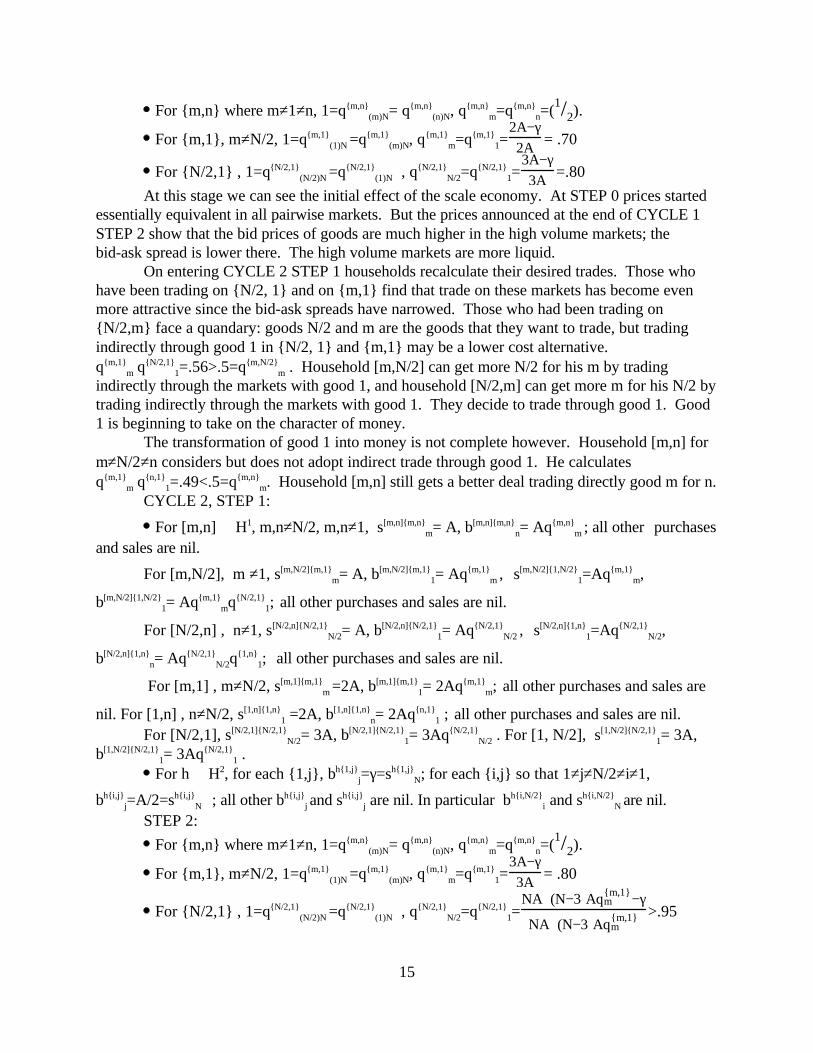
For {m,n} where m≠1≠n, 1=q{m,n}(m)N= q{m,n}

(n)N, q{m,n}m=q{m,n}

n=(1/2). For {m,1}, m≠N/2, 1=q{m,1}

(1)N =q{m,1}(m)N, q{m,1}

m=q{m,1}1= = .70 2A−γ

2A

For {N/2,1} , 1=q{N/2,1}(N/2)N =q{N/2,1}

(1)N , q{N/2,1}

N/2=q{N/2,1}1= =.80

3A−γ3A

At this stage we can see the initial effect of the scale economy. At STEP 0 prices startedessentially equivalent in all pairwise markets. But the prices announced at the end of CYCLE 1STEP 2 show that the bid prices of goods are much higher in the high volume markets; thebid-ask spread is lower there. The high volume markets are more liquid.

On entering CYCLE 2 STEP 1 households recalculate their desired trades. Those whohave been trading on {N/2, 1} and on {m,1} find that trade on these markets has become evenmore attractive since the bid-ask spreads have narrowed. Those who had been trading on{N/2,m} face a quandary: goods N/2 and m are the goods that they want to trade, but tradingindirectly through good 1 in {N/2, 1} and {m,1} may be a lower cost alternative.q{m,1}

m⋅q{N/2,1}1=.56>.5=q{m,N/2}

m . Household [m,N/2] can get more N/2 for his m by tradingindirectly through the markets with good 1, and household [N/2,m] can get more m for his N/2 bytrading indirectly through the markets with good 1. They decide to trade through good 1. Good1 is beginning to take on the character of money.

The transformation of good 1 into money is not complete however. Household [m,n] form≠Ν/2≠n considers but does not adopt indirect trade through good 1. He calculates q{m,1}

m⋅q{n,1}1=.49<.5=q{m,n}

m. Household [m,n] still gets a better deal trading directly good m for n.CYCLE 2, STEP 1:

For [m,n] ∈ H1, m,n≠N/2, m,n≠1, s[m,n]{m,n}m= A, b[m,n]{m,n}

n= Aq{m,n}m ; all other purchases

and sales are nil. For [m,N/2], m ≠1, s[m,N/2]{m,1}

m= A, b[m,N/2]{m,1}1= Aq{m,1}

m , s[m,N/2]{1,N/2}1=Aq{m,1}

m,

b[m,N/2]{1,N/2}1= Aq{m,1}

mq{N/2,1}1; all other purchases and sales are nil.

For [N/2,n] , n≠1, s[N/2,n]{N/2,1}N/2= A, b[N/2,n]{N/2,1}

1= Aq{N/2,1}N/2 , s[N/2,n]{1,n}

1=Aq{N/2,1}N/2,

b[N/2,n]{1,n}n= Aq{N/2,1}

N/2q{1,n}

1; all other purchases and sales are nil.

For [m,1] , m≠N/2, s[m,1]{m,1}m =2A, b[m,1]{m,1}

1= 2Aq{m,1}m; all other purchases and sales are

nil. For [1,n] , n≠N/2, s[1,n]{1,n}1 =2A, b[1,n]{1,n}

n= 2Aq{n,1}1 ; all other purchases and sales are nil.

For [N/2,1], s[N/2,1]{N/2,1}N/2= 3A, b[N/2,1]{N/2,1}

1= 3Aq{N/2,1}N/2 . For [1, N/2], s[1,N/2]{N/2,1}

1= 3A,b[1,N/2]{N/2,1}

1= 3Aq{N/2,1}1 .

For h ∈ H2, for each {1,j}, bh{1,j}j=γ=sh{1,j}

N; for each {i,j} so that 1≠j≠N/2≠i≠1,

bh{i,j}j=A/2=sh{i,j}

N ; all other bh{i,j}j and sh{i,j}

j are nil. In particular bh{i,N/2}i and sh{i,N/2}

N are nil.STEP 2: For {m,n} where m≠1≠n, 1=q{m,n}

(m)N= q{m,n}(n)N, q{m,n}

m=q{m,n}n=(1/2).

For {m,1}, m≠N/2, 1=q{m,1}(1)N =q{m,1}

(m)N, q{m,1}m=q{m,1}

1= = .80 3A−γ3A

For {N/2,1} , 1=q{N/2,1}(N/2)N =q{N/2,1}

(1)N , q{N/2,1}

N/2=q{N/2,1}1= >.95

NA+(N−3)Aqm{m,1}−γ

NA+(N−3)Aqm{m,1}

15

As CYCLE 2 STEP 1 is completed, trade has become partially monetized. All trade ingood N/2 goes through good 1 as a medium of exchange. As STEP 2 is completed, prices reflectthe higher trading volumes on markets including 1. Going into CYCLE 3 STEP 1, typical [m,n]for 1≠m≠N/2≠n≠1, can reconsider whether to trade in goods m and n directly or to trade throughgood 1 as a medium of exchange. In order to make that decision he compares q{m,n}

m to theproduct q{n,1}

1⋅q{m,1}

m. The former is the value of m in terms of n in direct trade, the latter throughtrade mediated by good 1. This is the same comparison [m,n] made at CYCLE 2 STEP 1, anddecided to continue to trade directly. But at the new posted prices we have .5 =q{m,n}

m < .64 = q{n,1}1⋅q

{m,1}m . It is more advantageous to trade indirectly. The outcome of

CYCLE 3 STEP 1 will be full monetization; all trade will go through good 1. CYCLE 3, STEP 1:

For [m,n] ∈ H1, m,n≠1, s[m,n]{m,1}m= A, b[m,n]{m,1}

1= Aq{m,1}m, s[m,n]{1,n}

1= Aq{m,1}m,

b[m,n]{1,n}n=A(q{m,1}

mq{n,1}1); all other purchases and sales are nil.

For [m,1] ∈ H1, m≠1, s[m,1]{m,1}m = 2A, b[m,1]{m,1}

1= 2Aq{m,1}m; all other purchases and sales

are nil. For [1,n] ∈ H1, n≠1, s[1,n]{1,n}1= 2A, b[1,n]{1,n}

n= 2Aq{1,n}1 ; all other purchases and sales are

nil. For [N/2,1], s[N/2,1]{N/2,1}

N/2= 3A, b[N/2,1]{N/2,1}1= 3Aq{N/2,1}

N/2 . For [1, N/2], s[1,N/2]{N/2,1}1= 3A,

b[1,N/2]{N/2,1}1= 3Aq{N/2,1}

1 .

For h ∈ H2, for each {i,j} with i≠1≠j, all transactions are nil. For {1,j}, 2≤ j ≤ N-1, bh{1,j}

j=γ=sh{i,j}N .

STEP 2: For {m,n} where m≠1≠n, 1=q{m,n}

(m)N= q{m,n}(n)N, q{m,n}

m=q{m,n}n=(1/2).

For {m,1}, m≠N/2, 1=q{m,1}(1)N =q{m,1}

(m)N, q{m,1}m=q{m,1}

1= > .914 (N−1)A+(N−3)Aqm{m,1}−γ

(N−1)A+(N−3)Aqm{m,1}

For {N/2,1} , 1=q{N/2,1}(N/2)N =q{N/2,1}

(1)N , q{N/2,1}

N/2=q{N/2,1}1= >.952

NA+(N−3)Aqm{m,1}−γ

NA+(N−3)Aqm{m,1}

CYCLE 4, STEP 1: Repeat Cycle 3, Step 1STEP 2: Repeat Cycle 3, Step 2CONVERGENCE.

What's happening in Example IV? Preferences and endowments are structured so that atroughly the same prices for all goods, there is a balance between supply and demand. Some pairsof goods are more actively traded than others. Good 1 has approximately twice as much activedemand (and supply) than most other goods. Good N/2 has slightly more active trade than mostother goods, and that active trade is concentrated in a supplier who demands good 1 and ademander endowed with good 1.

Here's how trade takes place. The starting point is a barter economy, the full array of(N-1)(N-2)/2 trading posts. For every pair of goods (i,j), where 1≤ i,j ≤ N-1, there is a postwhere that pair can be traded. The starting prices are chosen (somewhat arbitrarily) to coveraverage costs at low trading volume. The bid-ask spread is uniform across trading posts so tradeat each post is as attractive as anywhere else. Then each household computes its demands andsupplies at those prices. It figures out what it wants to buy and sell and to which trading posts it

16

should go to implement the trades. Since all bid-ask spreads start out equal, each household justgoes to the post that trades in the pair of goods that the household wants to exchange for oneanother; demanders of good j who are endowed with good i go to {i,j}. Because of thedistribution of demands and supplies, there is twice the trading volume on posts {1,j} than onmost {i,j} and three times as much on {1,N/2}.

Then the average cost pricing auctioneer responds to the planned transactions. He pricesbid/ask spreads in all markets to cover the costs of the trade on them. Since there is a scaleeconomy in the transactions technology, this leads to slightly narrower bid/ask spreads on the{1,j} markets and an even narrower spread on the {1, N/2} market. The auctioneer announceshis prices.

Households respond to the new prices. Households who want to buy or sell good N/2discover that the bid/ask spread on market {1, N/2} is lower than on any other market tradingN/2. It makes sense to channel transactions through this low cost market, even if the householdhas to undertake additional transactions to do so. Ordinarily households [i,N/2] and [N/2,i]would have gone directly to the market {i,N/2} to do their trading. But the combined transactioncosts on {i,1} and on {1,N/2} are lower than those on {i,N/2}. Households [i,N/2] and [N/2,i]find that they incur lower transaction costs by trading through good 1 as an intermediary. Theyexchange i for 1 and 1 for N/2 (or N/2 for 1 and 1 for i) rather than trade directly. The marketmakers on the many different {i,1} markets, 2 ≤ i ≤ N-1, find their trading volumes increased asthe [i,N/2] and [N/2,i] traders move their trades to {i,1} and {N/2,1}.

The average cost pricing auctioneer responds to the revised trading plans once again.Bid-ask spreads decline on {i,1}, 2 ≤ i ≤ N-1. Now the bid-ask spreads on {i,1} are less than halfthose on {i,j} for i≠1≠j. The auctioneer announces his prices.

Households respond to the new prices. For all households [i,j], it is now less expensive totrade through good 1 as an intermediary than to trade directly i for j or j for i. All [i,j] now tradeon {i,1} and {j,1}; none trade on {i,j}, for i≠1≠j. Trade is fully monetized with good 1 as the'money.'

The average cost pricing auctioneer re-prices the markets. Inactive markets, {i,j} fori≠1≠j, necessarily continue to post their starting prices (which reflected anticipated low tradingvolume). The active markets {i,1} get posted prices reflecting their high trading volumes, withnarrow bid-ask spreads.

Households review the newly posted prices. The narrow bid-ask spreads on the {i,1}markets reinforce the attractiveness of their previous plans, which called for trading through good1 as an intermediary. They leave their monetary trading plans in force. At current prices, it ismuch more economical to trade i for j by first trading i for 1 and then 1 for j than to trade i for jdirectly. High trading volumes on the {i,1} and {j,1} markets ensure low transaction costs andkeep them attractive. All trade takes place at {i,1}, i=2,3,4, ..., N-1. Good 1 has become theunique 'money'.

The economy of Example IV comes to precisely the opposite outcome if γi>NA for all i.Then there are no transaction cost scale economies in the relevant range. The equilibrium will benonmonetary direct barter trade.

17

V. Conclusion

Examples IV and III.3 demonstrate the following conception of the monetization of thetransactions process. Scale economies in the transactions technology mean that high volumemarkets will be low average cost markets. The transition from barter to monetary exchange is thetransition from a complex of many thin markets --- one for trade of each pair of goods for oneanother to an array of a smaller number of thick markets dealing in each good versus a uniquecommon medium of exchange. This transition is resource saving if the scale economies intransactions technology are large enough.

In section IV, with full double coincidence of wants, the emphasis is on scale economiesalone; high volume imparts liquidity and monetization. The example shows that the transitionprogresses through individually rational decisions when prices reflect the scale economy and theinitial condition includes one good (the latent 'money') with a relatively high transaction volume(hence low average transaction cost). Then, as Einzig notes, "favourite means of barter are aptto arise" and a barter economy thus converges incrementally to a monetary economy.

Conversely, section III emphasizes absence of double coincidence of wants. This settingnecessarily generates higher trading volumes to fulfill budget balance (T.ii) and achieve anequilibrium allocation. A demand for carriers of purchasing power between trading postsendogenously arises and focuses on low transaction cost goods, the 'natural' moneys. Absentscale economy there is no impetus for uniqueness of 'money.'

Scale economy is not a necessary condition for uniqueness of the medium of exchange inequilibrium (Example III.1), but scale economy helps to ensure uniqueness. If there is a uniquelow transaction cost instrument in an economy with a linear transaction cost structure, that naturalmoney may be the unique medium of exchange in equilibrium. If there are many equally low costcandidates for the medium of exchange, scale economy in transaction costs will allow one to beendogenously chosen as the unique medium of exchange. Inherent low cost and marketdetermined high volume combine to yield unique monetization. Menger (1892) describes thistransition:

when any one has brought goods not highly saleable to market, the idea uppermostin his mind is to exchange them, not only for such as he happens to be in need of,but...for other goods...more saleable than his own...By...a mediate exchange, hegains the prospect of accomplishing his purpose more surely and economically thanif he had confined himself to direct exchange...Men have been led...withoutconvention, without legal compulsion,...to exchange...their wares...for othergoods...more saleable...which ...have ...become generally acceptable media ofexchange.

Thus, Menger argues that starting from a relatively primitive market setting, some goods will bemore liquid than others. As they are adopted as media of exchange, markets for trade in themversus other goods become increasingly liquid. Eventually they become the common media ofexchange in equilibrium. Examples III.3 and IV formalize this argument emphasizing that theincreasing liquidity develops endogenously as a result of scale economy in the transaction process.

18

References

Banerjee, A. and E. Maskin (1996), "A Walrasian Theory of Money and Barter," QuarterlyJournal of Economics, v. CXI, n. 4, November, pp. 955-1005.

Clower, R. (1967), "A Reconsideration of the Microfoundations of Monetary Theory," WesternEconomic Journal, v. 6, pp. 1 - 8.

Clower, R. (1995), "On the Origin of Monetary Exchange," Economic Inquiry, v. 33, pp.525-536.

Einzig, P. (1966), Primitive Money, Oxford: Pergamon Press.Foley, D. K. (1970), "Economic Equilibrium with Costly Marketing," Journal of Economic

Theory, v. 2, n. 3, pp. 276 - 291.Hahn, F. H. (1971), "Equilibrium with Transaction Costs," Econometrica, v. 39, n. 3, pp. 417 -

439. Hahn, F. H. (1997), "Fundamentals," Revista Internazionale di Scienze Sociali, v. CV,

April-June, pp. 123-138. Iwai, K. (1995), "The Bootstrap Theory of Money: A Search Theoretic Foundation for Monetary

Economics," University of Tokyo, duplicated. Jevons, W. S. (1893), Money and the Mechanism of Exchange, New York: D. Appleton. Kiyotaki, N. and R. Wright (1989), "On Money as a Medium of Exchange," Journal of Political

Economy, v. 97, pp. 927 - 954. Li, Y., and R. Wright (1998), “Government Transaction Policy, Media of Exchange, and Prices,”

Journal of Economic Theory, v.81, pp. 290-313. Lerner, A. P. (1947), “Money as a Creature of the State,” Proceedings of the American

Economic Association, v. 37, pp. 312-317. Menger, C. (1892), "On the Origin of Money," Economic Journal, v. II, pp. 239-255. Translated

by Caroline A. Foley. Reprinted in R. Starr, ed., General Equilibrium Models ofMonetary Economies, San Diego: Academic Press, 1989.

Ostroy, J. and R. Starr (1990), "The Transactions Role of Money," in B. Friedman and F. Hahn,eds., Handbook of Monetary Economics, New York: Elsevier North Holland.

Ostroy, J. and R. Starr (1974), "Money and the Decentralization of Exchange," Econometrica, v.42, pp. 597 -610.

Rajeev, M. (forthcoming), "Marketless Set-Up vs Trading Posts: A Comparative Analysis"Annales d’Economie et de Statistique.

Smith, A. (1776), Wealth of Nations, Volume I, Book II, Chap. II. Starr, R. M. (1974), “The Price of Money in a Pure Exchange Monetary Economy with

Taxation,” Econometrica, v. 42, pp. 45-54. Starr, R. M. and M. B. Stinchcombe (1999), "Exchange in a Network of Trading Posts," in

Markets, Information, and Uncertainty: Essays in Economic Theory in Honor of KennethArrow, G. Chichilnisky, ed., Cambridge University Press.

Starr, R. M. and M. B. Stinchcombe (1998), "Monetary Equilibrium with Pairwise Trade andTransaction Costs," University of California, San Diego, duplicated.

Starrett, D. A. (1973), "Inefficiency and the Demand for Money in a Sequence Economy," Reviewof Economic Studies, v. XL, n. 4, pp. 437 -448.

19

Tobin, J. (1980), "Discussion," in Kareken, J. and N. Wallace, Models of Monetary Economies,Minneapolis: Federal Reserve Bank of Minneapolis.

Tobin, J. with S. Golub (1998), Money, Credit, and Capital, Boston: Irwin/McGraw-Hill. Walras, L. (1874), Elements of Pure Economics, Jaffe translation (1954), Homewood, Illinois:

Irwin.

20