university of california, irvine modeling of multivariate … · 2006-08-18 · university of...

UNIVERSITY OF CALIFORNIA,

IRVINE

Modeling of Multivariate Time Series

Using Hidden Markov Models

DISSERTATION

submitted in partial satisfaction of the requirements

for the degree of

DOCTOR OF PHILOSOPHY

in Information and Computer Science

by

Sergey Kirshner

Dissertation Committee:

Professor Padhraic Smyth, Chair

Professor Rina Dechter

Professor Richard Granger

Professor Max Welling

2005

The dissertation of Sergey Kirshner

is approved and is acceptable in quality

and form for publication on microfilm:

Committee Chair

University of California, Irvine

2005

ii

TABLE OF CONTENTS

LIST OF FIGURES viii

LIST OF TABLES xvii

ACKNOWLEDGMENTS xviii

CURRICULUM VITAE xix

ABSTRACT OF THE DISSERTATION xx

1 Introduction 1

1.1 Application: Multi-Site Precipitation Modeling . . . . . . . . . . . . . 2

1.2 High Level Overview of Related Work . . . . . . . . . . . . . . . . . . 9

1.3 Contributions . . . . . . . . . . . . . . . . . . . . . . . . . . . . . . . 9

1.4 Thesis Outline . . . . . . . . . . . . . . . . . . . . . . . . . . . . . . . 10

2 Preliminaries 13

2.1 Notation . . . . . . . . . . . . . . . . . . . . . . . . . . . . . . . . . . 13

2.2 Brief Introduction to Graphical Models . . . . . . . . . . . . . . . . . 14

2.2.1 Markov Networks . . . . . . . . . . . . . . . . . . . . . . . . . 15

2.2.2 Bayesian Networks . . . . . . . . . . . . . . . . . . . . . . . . 17

2.2.3 Decomposable Models . . . . . . . . . . . . . . . . . . . . . . 19

iii

2.2.4 Notes on Graphical Models . . . . . . . . . . . . . . . . . . . 20

3 A Review of Homogeneous and Non-Homogeneous Hidden Markov

Models 21

3.1 Model Description . . . . . . . . . . . . . . . . . . . . . . . . . . . . 21

3.1.1 Auto-regressive Models . . . . . . . . . . . . . . . . . . . . . . 23

3.1.2 Non-homogeneous HMMs . . . . . . . . . . . . . . . . . . . . 25

3.2 Hidden State Distributions . . . . . . . . . . . . . . . . . . . . . . . . 27

3.2.1 Inference . . . . . . . . . . . . . . . . . . . . . . . . . . . . . . 27

3.2.2 Sampling . . . . . . . . . . . . . . . . . . . . . . . . . . . . . 28

3.2.3 Most Likely Sequences . . . . . . . . . . . . . . . . . . . . . . 30

3.3 Learning . . . . . . . . . . . . . . . . . . . . . . . . . . . . . . . . . . 31

3.3.1 EM Framework for NHMMs . . . . . . . . . . . . . . . . . . . 31

3.4 Modeling Emission Distributions . . . . . . . . . . . . . . . . . . . . 36

3.5 Historical Remarks and Connections to Other Models . . . . . . . . . 40

3.6 Summary . . . . . . . . . . . . . . . . . . . . . . . . . . . . . . . . . 42

4 Parsimonious Models for Multivariate Distributions for Categorical

Data 43

4.1 Independence and Conditional Independence Models . . . . . . . . . 46

4.1.1 Auto-regressive Conditional Independence . . . . . . . . . . . 47

4.2 Tree-based Approximations . . . . . . . . . . . . . . . . . . . . . . . 48

4.2.1 Conditional Chow-Liu Forests . . . . . . . . . . . . . . . . . . 51

4.3 Beyond Trees . . . . . . . . . . . . . . . . . . . . . . . . . . . . . . . 57

4.3.1 Learning Parameters of Maximum Entropy Models . . . . . . 63

4.3.2 Product of Univariate Conditional MaxEnt Model . . . . . . . 68

4.3.3 Connection Between MaxEnt and PUC-MaxEnt Models . . . 71

iv

4.3.4 Selection of Features . . . . . . . . . . . . . . . . . . . . . . . 78

4.3.5 PUC-MaxEnt Models for Bivariate Interactions of Binary Data 80

4.4 Other Possibilities . . . . . . . . . . . . . . . . . . . . . . . . . . . . . 83

4.4.1 Multivariate Probit Model . . . . . . . . . . . . . . . . . . . . 83

4.4.2 Mixtures . . . . . . . . . . . . . . . . . . . . . . . . . . . . . . 88

4.5 Summary . . . . . . . . . . . . . . . . . . . . . . . . . . . . . . . . . 91

5 Models for Multivariate Real-Valued Distributions 92

5.1 Independence . . . . . . . . . . . . . . . . . . . . . . . . . . . . . . . 92

5.1.1 Modeling Daily Rainfall Amounts . . . . . . . . . . . . . . . . 93

5.2 Multivariate Normal Distributions . . . . . . . . . . . . . . . . . . . . 94

5.2.1 Unconstrained Normal Distribution . . . . . . . . . . . . . . . 95

5.2.2 Tree-Structured Normal Distributions . . . . . . . . . . . . . . 97

5.2.3 Learning Structure of Tree-Structured Normal Distributions . 103

5.3 Summary . . . . . . . . . . . . . . . . . . . . . . . . . . . . . . . . . 105

6 Putting It All Together: HMMs with Multivariate Emission Models106

6.1 HMM with Conditional Independence . . . . . . . . . . . . . . . . . . 107

6.1.1 AR-HMM with Conditional Independence . . . . . . . . . . . 110

6.1.2 Application to Multi-Site Precipitation Modeling . . . . . . . 112

6.2 HMM with Chow-Liu Trees . . . . . . . . . . . . . . . . . . . . . . . 114

6.2.1 HMM with Tree-Structured Normals . . . . . . . . . . . . . . 116

6.3 HMM with Emission Models of Higher Complexity . . . . . . . . . . 116

6.3.1 HMM with Full Bivariate MaxEnt . . . . . . . . . . . . . . . . 117

6.3.2 HMM with Saturated Normal Distributions . . . . . . . . . . 118

6.3.3 HMM with Product of Univariate Conditional MaxEnt Distri-

butions . . . . . . . . . . . . . . . . . . . . . . . . . . . . . . . 118

v

6.4 Summary . . . . . . . . . . . . . . . . . . . . . . . . . . . . . . . . . 120

7 Experimental Results: Sensitivity of Learning HMMs for Multivari-

ate Binary Data 123

7.1 Experimental Setup . . . . . . . . . . . . . . . . . . . . . . . . . . . . 124

7.2 Results . . . . . . . . . . . . . . . . . . . . . . . . . . . . . . . . . . . 128

7.2.1 First Set of Experiments . . . . . . . . . . . . . . . . . . . . . 128

7.2.2 Second Set of Experiments . . . . . . . . . . . . . . . . . . . . 133

7.3 Summary . . . . . . . . . . . . . . . . . . . . . . . . . . . . . . . . . 134

8 Experimental Results: Large Scale Study of Precipitation Modeling

for Different Geographic Regions 138

8.1 Related Work on Multi-site Precipitation Occurrence Modeling . . . . 139

8.2 Model Selection and Evaluation of the Results . . . . . . . . . . . . . 141

8.3 Performance Analysis on Geographic Regions . . . . . . . . . . . . . 142

8.3.1 Ceara Region of Northeastern Brazil . . . . . . . . . . . . . . 142

8.3.2 Southwestern Australia . . . . . . . . . . . . . . . . . . . . . . 151

8.3.3 Western United States . . . . . . . . . . . . . . . . . . . . . . 161

8.3.4 Queensland (Northeastern Australia) . . . . . . . . . . . . . . 168

8.4 Summary . . . . . . . . . . . . . . . . . . . . . . . . . . . . . . . . . 173

9 Summary and Future Directions 174

9.1 List of Contributions . . . . . . . . . . . . . . . . . . . . . . . . . . . 174

9.2 Future Directions . . . . . . . . . . . . . . . . . . . . . . . . . . . . . 177

Bibliography 180

Appendices 194

vi

A Conjugate Gradient Algorithm for Optimization . . . . . . . . . . . . 194

A.1 Optimization of Transition Parameters for NHMM . . . . . . 194

A.2 Optimization for Univariate Conditional MaxEnt Models . . . 196

B Proofs of Theorems . . . . . . . . . . . . . . . . . . . . . . . . . . . . 199

C Experimental Setup . . . . . . . . . . . . . . . . . . . . . . . . . . . . 201

vii

LIST OF FIGURES

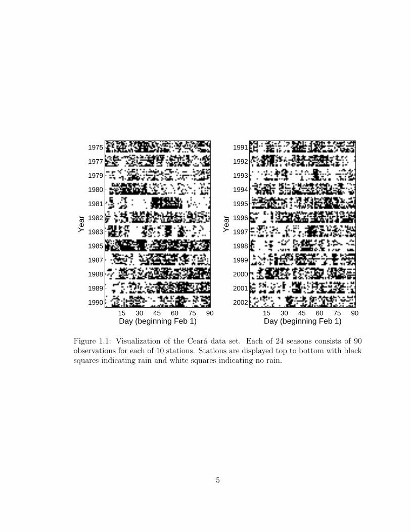
1.1 Visualization of the Ceara data set. Each of 24 seasons consists of

90 observations for each of 10 stations. Stations are displayed top to

bottom with black squares indicating rain and white squares indicating

no rain. . . . . . . . . . . . . . . . . . . . . . . . . . . . . . . . . . . 5

1.2 A map of Ceara region with rainfall station locations (left) and prob-

ability of precipitation (right). The stations are (with elevation): (1)

Acopiara (317 m), (2) Aracoiaba (107 m), (3) Barbalha (405 m), (4)

Boa Viagem (276 m), (5) Camocim (5 m), (6) Campos Sales (551

m), (7) Caninde (15 m), (8) Crateus (275 m), (9) Guaraciaba Do

Norte (902 m), and (10) Ibiapina (878 m). Circle radius denotes the

February–April climatological daily rainfall probability for 1975–2002. 6

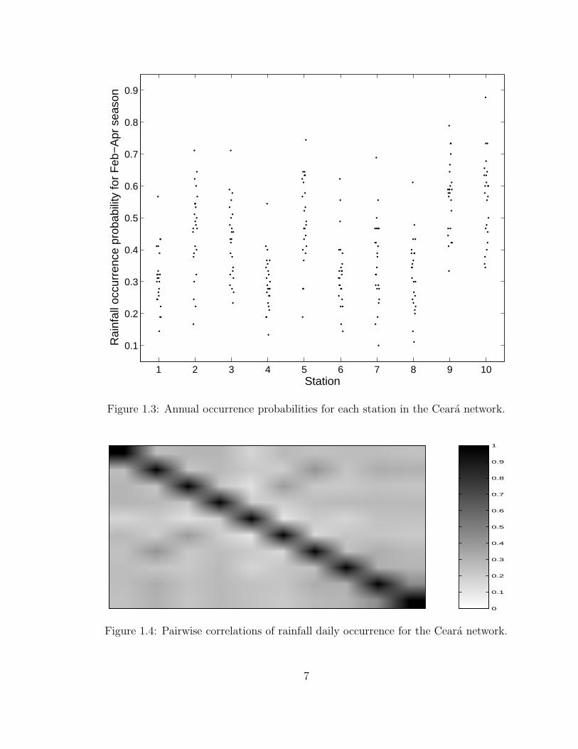
1.3 Annual occurrence probabilities for each station in the Ceara network. 7

1.4 Pairwise correlations of rainfall daily occurrence for the Ceara network. 7

1.5 Spell length distribution per station for the Ceara network. Stations

are displayed left-to-right and top-to-bottom (e.g., first row contains

plots for stations 1,2,3). x-axes indicate spell length; y-axes indicate

probability of spell duration of greater or equal length. Dry spells are

displayed in solid (blue); wet spells are displayed in dashed (red). . . 8

viii

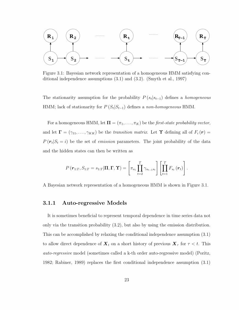
3.1 Bayesian network representation of a homogeneous HMM satisfying

conditional independence assumptions (3.1) and (3.2). (Smyth et al.,

1997) . . . . . . . . . . . . . . . . . . . . . . . . . . . . . . . . . . . . 23

3.2 Bayesian network representation of an AR-HMM satisfying conditional

independence assumptions (3.3) and (3.2). . . . . . . . . . . . . . . . 24

3.3 Bayesian network representation of a non-homogeneous HMM satisfy-

ing the conditional independence assumptions (3.1) (or, seen as dashed

lines, (3.3) for AR model) and (3.4). . . . . . . . . . . . . . . . . . . 25

3.4 Viterbi algorithm for finding most likely sequence of hidden states. . . 30

4.1 General conditional independence model (left) and correspondence

conditional independence model (right). . . . . . . . . . . . . . . . . . 48

4.2 Chow-Liu algorithm (very similar to Meila and Jordan, 2000). . . . . 50

4.3 Conditional Chow-Liu algorithm (Kirshner et al., 2004). . . . . . . . 52

4.4 Conditional CL forest for a hypothetical distribution with (a) 1 com-

ponent (b) 2 components (c) 3 components. . . . . . . . . . . . . . . 56

4.5 Markov Network for the MaxEnt model in (4.13). . . . . . . . . . . . 61

4.6 Efficient updating of MaxEnt parameters (similar to Bach and Jordan,

2002). . . . . . . . . . . . . . . . . . . . . . . . . . . . . . . . . . . . 64

4.7 Markov network for the Example 4.3 (left) and its junction tree (right). 66

4.8 Bayesian network for PUC-MaxEnt distribution in Example 4.4. . . . 76

4.9 Feature selection for exponential models. . . . . . . . . . . . . . . . . 79

4.10 Structure and parameter learning for PUC-MaxEnt. . . . . . . . . . . 82

ix

4.11 Bivariate probit distribution with β1 = 0.5, β2 = −1, and correlation

σ12 = 0.5. The probabilities for each of four pairs of values are equal

to the probability mass of the Gaussian in the corresponding quad-

rant: P (X1 = 1, X2 = 1) = 0.1462, P (X1 = 1, X2 = −1) = 0.5423,

P (X1 = −1, X2 = 1) = 0.0124, and P (X1 = −1, X2 = −1) = 0.2961. 86

4.12 Example of potential benefits of latent variables. If a latent variableXs

is included in the model, the Bayesian network (a) of the distribution

is sparser and requires fewer parameters than if Xs is ignored (network

(b)). . . . . . . . . . . . . . . . . . . . . . . . . . . . . . . . . . . . . 88

5.1 Illustration of the unique path property of the tree. For two nodes

u, v ∈ V, there is a unique neighbor z of u on the path from u to v. . 100

6.1 Bayesian network for a hypothetical (a) HMM-CI; (b) HMM-CL or

HMM-CL-Normal; (c) HMM-Full-MaxEnt or HMM-Full-Normal; (d)

HMM-PUC-MaxEnt . . . . . . . . . . . . . . . . . . . . . . . . . . . 109

6.2 Bayesian network for a hypothetical (a) HMM-Chains; (b) HMM-

CCL; (c) AR-HMM-PUC-MaxEnt . . . . . . . . . . . . . . . . . . . . 111

7.1 Estimated average negated normalized entropy ln P (D)NKLTM

of the test

models as a function of the number of hidden states K for the first

experimental setup. The lines correspond to models HMM-CI and

HMM-CL with high, moderate, and low average estimated entropy

(denoted by h,m, and l, respectively). Also plotted the lower bound

on the negated normalized entropy, − ln 2. . . . . . . . . . . . . . . . 127

x

7.2 Estimated normalized KL-divergences for HMM-CI (top) and HMM-

CL (bottom) with high (left), moderate (center), and low (right) av-

erage estimated entropy as a function of the number of hidden states.

Curves on each plot correspond to different values of the number of

sequences N . . . . . . . . . . . . . . . . . . . . . . . . . . . . . . . . 130

7.3 Contour plots of the probability that KLnorm ≤ τ (τ = 0.005) for

HMM-CI (left) and HMM-CL (right) with high entropy (top), mod-

erate entropy (center), and low entropy (bottom). . . . . . . . . . . . 131

7.4 Upper bounds on the proportion of correctly learned edges for HMM-

CL with high (left), moderate (center), and low (right) entropies as a

function of the number of hidden states. Curves on each plot corre-

spond to different values of the number of sequences N . . . . . . . . . 132

7.5 Estimated normalized KL-divergences for HMM-CI (top left), HMM-

CL(top center), HMM-PUC-MaxEnt (top right), HMM-Chains (bot-

tom left), HMM-CCL (bottom center), and AR-HMM-PUC-MaxEnt

(bottom right) as a function of the number of hidden states. Curves

on each plot correspond to different values of the number of sequences

N . . . . . . . . . . . . . . . . . . . . . . . . . . . . . . . . . . . . . . 135

7.6 Upper bounds on the proportion of correctly learned edges for HMM-

CL (left) and HMM-CCL (right) as a function of the number of hidden

states. Curves on each plot correspond to different values of the num-

ber of sequences N . . . . . . . . . . . . . . . . . . . . . . . . . . . . . 136

7.7 Estimated normalized KL-divergences for different models for estima-

tion the parameters of a HMM-CI based on 24 sequences (left) and 100

sequences (right). Curves on each plot correspond to different models. 136

xi


tion the parameters of a HMM-CL based on 24 sequences (left) and

100 sequences (right). Curves on each plot correspond to different

models. . . . . . . . . . . . . . . . . . . . . . . . . . . . . . . . . . . 137


tion the parameters of a HMM-CCL based on 24 sequences (left) and

100 sequences (right). Curves on each plot correspond to different

models. . . . . . . . . . . . . . . . . . . . . . . . . . . . . . . . . . . 137

8.1 Precipitation persistence for Ceara set. Each point corresponds to a

value for one season. . . . . . . . . . . . . . . . . . . . . . . . . . . . 143

8.2 Ceara data: average out-of-sample log-likelihood obtained by a leave-

one-out cross-validation for various models across a number of hidden

states. . . . . . . . . . . . . . . . . . . . . . . . . . . . . . . . . . . . 145

8.3 Ceara data: average out-of-sample absolute difference between the

statistics of the simulated data and the left-out data as determined

by leave-six-out cross-validation for correlation (top) and persistence

(bottom). . . . . . . . . . . . . . . . . . . . . . . . . . . . . . . . . . 148

8.4 Weather states obtained by training 4-state HMM-CI on the Ceara

set. Circle radii indicate the precipitation probability for each station

given the state. . . . . . . . . . . . . . . . . . . . . . . . . . . . . . . 149

8.5 Ceara data: correlation matrix of rainfall daily occurrence (left), ab-

solute difference between the correlation matrix of the data and the

correlation of the data simulated from a 4-state HMM-CI (middle)

and a 3-state HMM-CL (right). The average absolute difference for

non-diagonal entries is 0.020 for HMM-CI and 0.010 for HMM-CL. . . 150

xii

8.6 Ceara data: scatter plot of the precipitation probabilities (left) and

the persistence (right) for each station of the actual data versus the

simulated data from various models. Straight lines correspond to y = x.150

8.7 Stations in the Southwestern Australia region. Circle radii indicate

marginal probabilities of rainfall (> 0.3mm) at each location. . . . . . 151

8.8 Southwestern Australia data: average out-of-sample log-likelihood ob-

tained by a leave-one-out cross-validation for various models across a

number of hidden states. . . . . . . . . . . . . . . . . . . . . . . . . . 152

8.9 Southwestern Australia data: scatter plot of scaled log-likelihoods

(left) and average prediction error (right) obtained by leaving one-

winter-out cross-validation. Straight lines correspond to y = x. . . . . 153

8.10 Southwestern Australia data: correlation matrix of rainfall daily oc-

currence (left), absolute difference between the correlation matrix of

the data and the correlation of the data simulated from a 3-state

HMM-PUC-MaxEnt (right). The average absolute difference for non-

diagonal entries is 0.025. . . . . . . . . . . . . . . . . . . . . . . . . . 156

8.11 Southwestern Australia data: scatter plot of the precipitation proba-

bilities (left) and the persistence (right) for each station of the actual

data versus the simulated data from various models. Straight lines

correspond to y = x. . . . . . . . . . . . . . . . . . . . . . . . . . . . 156

8.12 Graphical interpretation of the hidden states for a 5-state HMM-CL

trained on Southwestern Australia data. Circle radii indicate the pre-

cipitation probability for each station given the state. Lines between

the stations indicate the edges in the graph while different types of

lines indicate the strength of mutual information of the edges. . . . . 157

xiii

8.13 Graphical interpretation of the hidden states for a 5-state HMM-CI

model trained on Southwestern Australia data. Circle radii indicate

the precipitation probability for each station given the state. . . . . . 158

8.14 Graphical interpretation of the hidden states for a 5-state HMM-PUC-

MaxEnt model trained on Southwestern Australia data. Circle radii

indicate the precipitation probability for each station given the state.

Links between the stations indicate the edges in the graph. . . . . . . 159

8.15 Graphical interpretation of the hidden states for a 5-state HMM-CCL

trained on Southwestern Australia data. Circle radii indicate the pre-

cipitation probability for each station given the state. Lines between

the stations indicate the edges in the graph while different types of

lines indicate the strength of mutual information of the edges. The

left side of the plot corresponds to observations Rt−1 while the right

side to Rt. . . . . . . . . . . . . . . . . . . . . . . . . . . . . . . . . . 160

8.16 Stations in the Western U.S. region. Circle radii indicate marginal

probabilities of rainfall (> 0mm) at each location. . . . . . . . . . . . 161

8.17 Western U.S. data: average out-of-sample log-likelihood for various

models across a number of hidden states. Straight lines correspond

to scaled log-likelihoods of DBNs with transition determined by the

corresponding conditional distribution. . . . . . . . . . . . . . . . . . 163

8.18 Western U.S. data: scatter plot of scaled log-likelihoods (left) and

average prediction error (right) obtained by leaving one-winter-out

cross-validation. Lines correspond to y = x. . . . . . . . . . . . . . . 163

xiv

8.19 Graphical interpretation of the hidden states for a 7-state HMM-CCL

trained on Western U.S. data. Circle radii indicate the precipitation

probability for each station given the state. Lines between the stations

indicate the edges in the graph while different types of lines indicate

the strength of mutual information of the edges. The left side of the

plot corresponds to observations Rt−1 while the right side to Rt. . . . 165

8.20 Graphical interpretation of the hidden states for a 6-state AR-HMM-

PUC-MaxEnt trained on Western U.S. data. Circle radii indicate the

precipitation probability for each station given the state. Edges be-

tween the stations indicate the edges in the graph. The left side of the


8.21 Western U.S. data: correlation matrix of rainfall daily occurrence

(left), absolute difference between the correlation matrix of the data

and the correlation of the data simulated from a 6-state AR-HMM-

PUC-MaxEnt (middle) and a 7-state HMM-CCL (right). The aver-

age absolute difference for non-diagonal entries is 0.019 for AR-HMM-

PUC-MaxEnt and 0.013 for HMM-CCL. . . . . . . . . . . . . . . . . 167

8.22 Western U.S. data: scatter plot of the precipitation probabilities (left)

and the persistence (right) for each station of the actual data versus

the simulated data from various models. Straight lines correspond to

y = x. . . . . . . . . . . . . . . . . . . . . . . . . . . . . . . . . . . . 167

8.23 Stations in the Queensland (Northeastern Australia) region. Circle

radii indicate marginal probabilities of rainfall (≥ 1mm) at each location.168

8.24 Queensland data: average out-of-sample log-likelihood for various mod-

els across different number of hidden states. . . . . . . . . . . . . . . 169

xv

8.25 Queensland data: average out-of-sample absolute difference of corre-

lation (left) and persistence (right) of the simulated data with the

left-out data statistics. . . . . . . . . . . . . . . . . . . . . . . . . . . 170

8.26 Graphical interpretation of the hidden states for a 4-state AR-HMM-

PUC-MaxEnt trained on Queensland data. Circle radii indicate the

precipitation probability for each station given the state. Edges be-

tween the stations indicate the edges in the graph. The left side of the


8.27 Queensland data: correlation matrix of rainfall daily occurrence (left),

absolute difference between the correlation matrix of the data and

the correlation of the data simulated from a 4-state AR-HMM-PUC-

MaxEnt (right). The average absolute difference for non-diagonal en-

tries is 0.013. . . . . . . . . . . . . . . . . . . . . . . . . . . . . . . . 172

8.28 Queensland data: scatter plot of the precipitation probabilities (left)

and the persistence (right) for each station of the actual data versus

the simulated data from various models. Straight lines correspond to

y = x. . . . . . . . . . . . . . . . . . . . . . . . . . . . . . . . . . . . 172

xvi

LIST OF TABLES

1.1 Models for multivariate categorical data. . . . . . . . . . . . . . . . . 12

6.1 Comparison of complexities of HMM models for multivariate time series122

8.1 Performance of HMM-CIs evaluated by leave-six-out cross-validation. 147

8.2 Performance of HMM-CIs evaluated by leave-one-out cross-validation. 147

8.3 Transition parameters for 4-state HMM-CI trained on Ceara data. . . 147

xvii

ACKNOWLEDGMENTS

I wish to thank my advisor Padhraic Smyth for his guidance and unconditional sup-

port during my years at UCI, and for teaching me so much. Padhraic, I do not know

whether anyone else would have gone as far to accommodate me as you did – thank

you! Good portion of the credit also belongs to my collaborator Andy Robertson for

making my research feel so much more tangible. I am very grateful to my commit-

tee, Max Welling, Rina Dechter, and Rick Granger, for insightful suggestions and

making sure I am not completely off-base. Special thanks to my collaborators from

Lawrence Livermore National Laboratory, Chandrika Kamath and Erick Cantu-Paz,

for involving me in their exciting project.

My graduate life would not have been the same without my officemate, Sridevi,

and everyone else in the Datalab, Dima, Dasha, Igor, Xianping, Scott G., Joshua,

Scott W., Seyoung, Naval, Chaitanya, Lucas, just to name a few. Thank you all for

making it great and memorable! I also wish to thank my graduate counselors, Kris

Bolcer and Mylena Wypchlak, for answering a million of repeating questions with

a welcoming smile; David Eppstein, Sandra Irani, and others in the theory group

for welcoming me when I first came to UCI; David Kay for pleasant conversations

and tips on teaching; Mike Dillencourt for memorable pizza nights while grading 6A

exams; staff at the grant and travel offices, especially Patty Jones, for making my

conference travel painless (well, mostly painless).

Finally, I owe a lot to my family; my parents for enduring my constant travel-

ing and just being there for me; my sister and her family for a friendly chat and

support whenever I need it; and most importantly, to my wife Julia for constant

encouragement and just the right amount of nagging.

xviii

CURRICULUM VITAE

Sergey Kirshner

Date of Birth: January 3, 1976 in Odessa, USSR

EducationPh.D. 03/2005 UC Irvine Information and Computer ScienceM.S. 12/2001 UC Irvine Information and Computer ScienceB.A. 05/1998 UC Berkeley Mathematics & Computer Science

Honors and AwardsRIACS Summer Student Research Program Grant, 2000Honorable mention at the 56th William Lowell Putnam Mathematical Competition (top2%), 1995

Professional Experience09/1999–present Research Assistant, School of ICS, UC Irvine, CA06-08/2002 Instructor, School of ICS, UC Irvine, CA09/2000–03/2001 Teaching Assistant, School of ICS, UC Irvine, CA06-09/2000 Student Research Scientist, RIACS/NASA ARC, Moffett Field, CA06/1998–08/1999 Systems Analyst, NASA Ames Research Center, Moffett Field, CA

Peer-Reviewed Publications ListA.W. Robertson, S. Kirshner, and P. Smyth, ’Daily rainfall occurrence over North-east Brazil and its downscalability using a hidden Markov model.’ Journal of Climate,17(22):4407–4424, 2004S. Kirshner, P. Smyth, A.W. Robertson, ’Conditional Chow-Liu tree structures formodeling discrete-valued vector time series,’ UAI-2004, pp. 317-324, 2004S. Kirshner, S. Parise, and P. Smyth, ’Unsupervised learning from permuted data,’ICML-2003, pp. 345-352, 2003S. Kirshner, I.V. Cadez, P. Smyth, and C. Kamath, ’Learning to classify galaxy shapesusing the EM algorithm,’ NIPS-2002, pp. 1497-1504, 2003S. Kirshner, I.V. Cadez, P. Smyth, C. Kamath, and E. Cantu-Paz, ’Probabilistic model-based detection of bent-double radio galaxies,’ ICPR-2002, vol.2, 2002, pp.499-502D. Wolpert, S. Kirshner, C. Merz, and K. Tumer, ’Adaptivity in agent-based routingfor data networks,’ Agents-2000, pp.396-403

xix

ABSTRACT OF THE DISSERTATION

Modeling of Multivariate Time Series

Using Hidden Markov Models

By

Sergey Kirshner

Doctor of Philosophy in Information and Computer Science

University of California, Irvine, 2005

Professor Padhraic Smyth, Chair

Vector-valued (or multivariate) time series data commonly occur in various sciences.

While modeling univariate time series is well-studied, modeling of multivariate time

series, especially finite-valued or categorical, has been relatively unexplored. In this

dissertation, we employ hidden Markov models (HMMs) to capture temporal and

multivariate dependencies in the multivariate time series data. We modularize the

process of building such models by separating the modeling of temporal dependence,

multivariate dependence, and non-stationary behavior. We also propose new meth-

ods of modeling multivariate dependence for categorical and real-valued data while

drawing parallels between these two seemingly different types of data. Since this

work is in part motivated by the problem of prediction precipitation over geographic

regions from the multiple weather stations, we present in detail models pertinent to

this hydrological application and perform a thorough analysis of the models on data

collected from a number of different geographic regions.

xx

Chapter 1

Introduction

High-dimensional multivariate data sets occur in a large number of problem do-

mains. In many cases, these data sets have either sequential or temporal structure.

For example, economics provides us with time series of stock or index prices; speech

and music patterns can be thought of as sequences of signals at different frequen-

cies; atmospheric scientists has been collecting measurements for locations all over

the planet for the last century. Modeling of and forecasting from such data is an

important problem in all of the respective areas. Thus, it is important to develop

efficient, accurate, and flexible data analysis techniques for multivariate time series

data.

While there is a significant volume of literature on time series modeling, the ma-

jority of it concerns with the univariate case. Extensions of real-valued univariate

models to vector observations often involve high-dimensional auto-covariance matri-

ces and are linear in structure (e.g., Brockwell and Davis, 2002; Shumway and Stoffer,

2000; Hamilton, 1994). Direct modeling of multivariate sequences for categorical data

typically requires an even larger number of parameters than the real-valued case since

1

we cannot use smoothness, linearity, or normality property of the real-valued data.

Modeling of vector series for finite domains is a relatively new research area, and tech-

niques such as dynamic Bayesian networks (Murphy, 2002) and dynamic graphical

models (e.g., West and Harrison, 1997) are being explored for this problem. Mixed

(both continuous- and discrete-valued) data modeling is even less explored due to

the difficulty of modeling interactions between finite- and real-valued variables.

The approach in this thesis is to model discrete-time multivariate time series data

using hidden Markov models (HMMs), a special class of dynamic Bayesian networks.

HMMs assume that the observed data is generated via finite-valued latent (unob-

served) process. This unobserved process is assumed to be in one of a finite number

of discrete states at each discrete time point and to transition stochastically in a

Markov fashion given the previous state or states. The observed data at each time

point depends only on the value of the corresponding hidden state and is indepen-

dent of the rest of the data. The HMM can be viewed as separating the temporal

and multivariate aspects of the data, with the Markov dependency capturing the

temporal property, and the static probability distribution of a vector at a given time

given the hidden state capturing multivariate dependencies.

1.1 Application: Multi-Site Precipitation Model-

ing

One of the main applications for the research in this thesis is modeling and predic-

tion of rainfall occurrences and amounts, across networks of locations. Precipitation

prediction is an important problem in hydrology and agriculture and has a long

history of research. Standard atmospheric modeling techniques are not particularly

2

effective for this type of problem since precipitation is a local process and can have

a large variance over time, i.e., precipitation can be unpredictable and have high en-

tropy. General circulation models (GCMs) (e.g., Randall, 2000), the most commonly

used tool for seasonal climate prediction, do not perform well in modeling local pre-

cipitation (e.g. Semenov and Porter, 1995) as they operate on a much coarser grid

(usually, 2.5 × 2.5) than the spatial scale of precipitation. Thus scientists often

employ statistical models based on historical precipitation data (possibly with other

atmospheric measurements and/or GCM predictions) for the task local precipitation

modeling and prediction. A short review of existing statistical method for precipita-

tion modeling can be found in Section 8.1.

One of the goals of this work is to develop tools for building statistical models for

multi-site daily precipitation. Due to high variance, we obviously cannot make accu-

rate predictions for a specific day and a specific location based just on the historical

data. We can, however, build generative models that can produce realistic simu-

lated daily rainfall sequences preserving observed occurrence (and amounts) correla-

tions between the stations, precipitation wet/dry spell durations, and can reasonably

predict how wet the predicted season would be given some additional atmospheric

information. Simulated runs of this model can be used to improve water resource

management or to influence decisions in crop planning. Of particular interest are

seasonal predictions and simulations, where the statistical characteristics of a winter

season (for example) are forecast by the model conditioned on the “state” of the

climate system at the start of the season.

To give a flavor of the problem, we preview a precipitation occurrence data set

collected from 10 rain stations in the Ceara region of Northeastern Brazil over wet

3

seasons of Feb–April (90 days beginning February 1) from 1975–2002, provided by

Fundaco Cearense de Meteorologia (FUNCEME; Figure 1.1). Four of the seasons

(1976, 78, 84, 86) contained significant number of missing observations and were

not considered. Figure 1.2 shows the locations of individual rain stations and their

daily rainfall occurrence probabilities, one of the data statistics we would like our

model to reproduce. As Figure 1.1 suggests, the data has very high variance; some

of the variability can be visualized by looking at seasonal occurrence probabilities

for each station (Figure 1.3). The problem of modeling this interannual variability

recurs throughout atmospheric sciences and is quite important. Another problem of

importance in this general context is modeling of spatial dependence — we employ

correlation1 as one of the measures of co-occurrence of rainfall for pairs of stations.

Figure 1.4 summarizes pairwise correlations collectively for all years in the data

set. Note that it is not sufficient to forecast the seasonal statistics of rainfall at a

single station as the spatial correlation structure should also be retained. Finally,

atmospheric scientists are interested in models matching the distribution of dry (and

sometimes, wet) spell lengths.2 These spell lengths for individual stations often

exhibit geometric behavior (Figure 1.5) as is well known in precipitation modeling

literature (e.g., Wilks and Wilby, 1999). Thus, the challenge is to develop methods

that can take as input data such as that shown in Figure 1.1 and produce predictions

for future seasons that are accurate across multiple statistical criteria (e.g., mean

occurrence, variability, spatial correlations, run lengths).

1Linear (Pearson’s) correlation is defined as ρxy = Cov(X,Y )√V ar(X)V ar(Y )

.

2A dry (wet) spell of length n is an event of n consecutive days without (with) precipitation.

4

Yea

r

Day (beginning Feb 1)15 30 45 60 75 90

1975

1977

1979

1980

1981

1982

1983

1985

1987

1988

1989

1990

Day (beginning Feb 1)

Yea

r

15 30 45 60 75 90

1991

1992

1993

1994

1995

1996

1997

1998

1999

2000

2001

2002

Figure 1.1: Visualization of the Ceara data set. Each of 24 seasons consists of 90observations for each of 10 stations. Stations are displayed top to bottom with blacksquares indicating rain and white squares indicating no rain.

5

318.5 319 319.5 320 320.5 321 321.5 322 322.5−8

−7.5

−7

−6.5

−6

−5.5

−5

−4.5

−4

−3.5

−3

−2.5

1

2

3

4

5

6

7

8

9

10

318.5 319 319.5 320 320.5 321 321.5 322 322.5−8

−7.5

−7

−6.5

−6

−5.5

−5

−4.5

−4

−3.5

−3

−2.5

0.2

0.4

0.6

Figure 1.2: A map of Ceara region with rainfall station locations (left) and probabilityof precipitation (right). The stations are (with elevation): (1) Acopiara (317 m), (2)Aracoiaba (107 m), (3) Barbalha (405 m), (4) Boa Viagem (276 m), (5) Camocim(5 m), (6) Campos Sales (551 m), (7) Caninde (15 m), (8) Crateus (275 m), (9)Guaraciaba Do Norte (902 m), and (10) Ibiapina (878 m). Circle radius denotes theFebruary–April climatological daily rainfall probability for 1975–2002.

6

1 2 3 4 5 6 7 8 9 10

0.1

0.2

0.3

0.4

0.5

0.6

0.7

0.8

0.9

Station

Rai

nfal

l occ

urre

nce

prob

abili

ty fo

r F

eb−

Apr

sea

son

Figure 1.3: Annual occurrence probabilities for each station in the Ceara network.

0

0.1

0.2

0.3

0.4

0.5

0.6

0.7

0.8

0.9

1

Figure 1.4: Pairwise correlations of rainfall daily occurrence for the Ceara network.

7

0 10 20 3010

−4

10−2

100

0 10 20 3010

−4

10−2

100

0 10 20 3010

−4

10−2

100

0 10 20 3010

−4

10−2

100

0 10 20 3010

−4

10−2

100

0 10 20 3010

−4

10−2

100

0 10 20 3010

−4

10−2

100

0 20 4010

−4

10−2

100

0 10 20 3010

−4

10−2

100

0 10 20 3010

−4

10−2

100

Figure 1.5: Spell length distribution per station for the Ceara network. Stations aredisplayed left-to-right and top-to-bottom (e.g., first row contains plots for stations1,2,3). x-axes indicate spell length; y-axes indicate probability of spell durationof greater or equal length. Dry spells are displayed in solid (blue); wet spells aredisplayed in dashed (red).

8

1.2 High Level Overview of Related Work

Table 1.1 provides a crude and somewhat incomplete overview of commonly used

models for multivariate categorical data with latent states. The x-axis in the table

indicates the type of model being used for the hidden states, and the y-axis indicates

the type of multivariate model being used on observations. By decomposing the

problem into (a) temporal latent structure and (b) multivariate observation models,

we can “cover” the space of different modeling possibilities within the general class

of HMM-type models.

Most of the previously studied models fall along the lines of learning of multivariate

structure without temporal component (left side of Table 1.1) or temporal structure

without multivariate component (top part of Table 1.1). The work in this thesis will

focuses on modeling both aspects, as reflected in the table.

1.3 Contributions

The primary novel contributions of this thesis are:

• The conditional Chow-Liu forest model and associated learning algorithm for

conditional probability distributions on multivariate categorical data (Section

4.2.1, Kirshner et al. (2004));

• Hidden Markov models with Chow-Liu trees and conditional Chow-Liu forests

and their learning algorithms for multivariate time series modeling (Section 6.2,

Kirshner et al. (2004));

• Derivation of analytic expressions for covariance matrices for multivariate tree-

structured Gaussian models (Section 5.2.2);

9

• Product of univariate conditional maximum entropy model and associated

learning algorithm for conditional probability distributions on multivariate cat-

egorical data; HMM with the above model for data distribution in each hidden

state (Sections 4.3.2, 4.3.5, 6.3.3);

• A new type of HMM for multi-site precipitation amount modeling (Section

6.1.2).

Other contributions are:

• Derivation of the update rules for the transition component of non-homoge-

neous HMMs (Appendix A.1, Robertson et al. (2003));

• Empirical study of the sensitivity of the parameter estimation to the amount

of training data (Section 7);

• Comprehensive empirical study of HMM performance on the precipitation data

(Chapter 8, Robertson et al. (2004); Kirshner et al. (2004));

1.4 Thesis Outline

Chapter 2 provides the basic notation and concepts of graphical models used

throughout the thesis. Chapter 3 introduces and provides an overview of hidden

Markov models. Chapter 4 describes models for the multivariate categorical data.

Chapter 5 deals with models on multivariate real-valued data concentrating on Gaus-

sian models and touching upon the exponential distributions. Chapter 6 ties up the

results from Chapters 4 and 5 to describe the main result of this thesis, HMM-based

multivariate time series models. Chapter 7 demonstrate the effectiveness of the mod-

els on simulated data while Chapter 8 applies the models to precipitation occurrence

10

data for several geographical regions. Finally, Chapter 9 summarizes the main results

and outlines remaining questions and possible future approaches.

11

Table 1.1: Models for multivariate categorical data.

Latent StructureMultivariateStructure

No Explicit Temporal Component Explicit Temporal Component

No Latent Variables Mixture Non-homogeneousMixture

HMM Non-homogeneousHMM

Univariate(Bernoulli)

e.g., Duda et al.(2000)

e.g., McLachlanand Peel (2000)

Jordanand Jacobs(1994)

Baum et al.(1970); Rabiner(1989)

Bengio and Frasconi(1995); Bengio andBengio (1996); Meilaand Jordan (1996)

ConditionalIndepen-dence

e.g., Duda et al.(2000)

e.g., McLachlanand Peel (2000)

Jordanand Jacobs(1994)

e.g., Zucchiniand Guttorp(1991)

Hughes and Guttorp(1994)

MultivariateProbit (bi-nary only)

e.g., Ashford andSowden (1970);Chib and Greenberg(1998)

Chow-LiuTrees

Chow and Liu (1968) Grim (1984); Meilaand Jordan (2000)

Kirshner et al.(2004), thesis

thesis

MaxEnt (ex-ponential)

Brown (1959); Dar-roch and Ratcliff(1972)

Pavlov et al. (2003) Hughes et al.(1999), thesis

Hughes et al. (1999),thesis

12

Chapter 2

Preliminaries

This chapter defines the notation and briefly describes some of the important

concepts used in the remainder of this thesis.

2.1 Notation

In the interest of consistency and for easier readability, we list here the general

notation adopted in the rest of the thesis. Deviations from this notation will be

mentioned prior to use.

Sets are denoted by calligraphic capital letters (e.g., X ,Y,Z, . . . ) except for when

the sets already have established symbols (e.g., R). Elements or members of sets

are denoted by lowercase roman letters (e.g., a ∈ A), and subsets are denoted by

uppercase roman letters (e.g., A ⊆ A).

All random variables are denoted in capital Roman letters (e.g., X, Y, Z, . . . );

in addition, multivariate or vector random variables are denoted in boldface (e.g.,

X,Y ,Z, . . . ). Values of random variables are denoted by lowercase letters with

13

vectors in boldface (e.g., X = x or X = x). Probability distributions defined on

the discrete-valued domains are denoted by P (e.g., P (X)) while probability den-

sity functions (PDFs) defined over continuous domains are denoted by p (X = x).

A probability distribution P (X) (or p (X)) value at a given point x P (X = x) will

be denoted by P (x) (or, respectively, p (x)) for short. For a vector random variable

X = (X1, . . . , XM), individual components or variables will be indexed by one of

two ways: (1) by a number 1, . . . ,M , e.g., X1 or Xi for i = 1, . . . ,M , or (2) by

an element of a set V consisting of M elements where each v ∈ V corresponds to

exactly one component of X, e.g., u ∈ V corresponds to Xu. The latter notation

also allows us to denote multiple variables from a vector random variable, e.g., if

A = a, b, c , XA = Xa, Xb, Xc. We will also use this index set notation for the

domain X of X, e.g., xA ∈ XA.

All vectors are assumed to be column vectors. A transpose of a vector x is denoted

by x′. A transpose of a matrix A is denoted by A′.

Individual model parameters are denoted by Greek letters (e.g., λ) while vector

model parameters and sets of model parameters are denoted by boldfaced Greek

letters (e.g., θ, Σ, υ).

2.2 Brief Introduction to Graphical Models

Since in this thesis we are dealing with multivariate probability distributions, it

is useful to describe a general framework for specifying the structure of conditional

independencies (and dependencies) between variables. We will use graphs with nodes

corresponding to variables, and edges corresponding to multivariate dependencies, to

represent the structure of the probability distributions. Such graphical models are

14

often called belief networks. We will briefly define a few types of commonly used

graphical models.

Let P be a distribution defined on an M -variate random variable

X = (X1, . . . , XM) where each Xi takes values on the domain Xi, and X takes

values on X = X1 × · · · × XM . Let V = v1, . . . , vM be a set of vertices or nodes

with each vi corresponding to random variable Xi. We will represent dependencies

between the variables in X by a graph G = (V, E) with edges E selected to capture

conditional independence of the variables of X . For disjoint A,B,C ⊆ V, we will say

that A and B are conditionally independent given C, denoted by A ⊥ B | C, if

P (xA,xB|xC) = P (xA|xC)P (xB|xC) , whenever P (xC) > 0.

Alternatively,

P (xA|xB,xC) = P (xA|xC) , when P (xB,xC) > 0.

2.2.1 Markov Networks

First, we briefly describe how to use undirected graphs to describe conditional inde-

pendence relations. Let G = (V, E) be an undirected graph with nodes V correspond-

ing to variables of X and a set of undirected edges E defined on

u, v ∈ V × V : u 6= v. The conditional independence relations of P can be en-

coded using a separation property. For three disjoint subsets A,B,C ⊆ V, C sepa-

rates A from B if any path connecting any a ∈ A and any b ∈ B passes through a

15

node from C. As in Pearl (1988), if ∀A,B,C ⊆ V

A ⊥ B | C =⇒ C separates A from B,

then G is a dependency map or D-map of P . Conversely, if separation in G implies

the conditional independence,

A ⊥ B | C ⇐= C separates A from B,

then G is an independency map or I-map of P . If both conditions hold, then G is a

perfect map of P . Since we are interested in capturing the conditional independency

relations for a distribution without introducing additional dependency assumptions,

we require that undirected graphical models be I-maps of P . Such graph always exists

as a graph with edges connecting all pairs of vertices, otherwise called a complete

graph, is an I-map. We further restrict our graph to be a minimal I-map of P by

requiring that a deletion of any e ∈ E would make G cease to be an I-map. Such G is

called a Markov network of P (Pearl, 1988). Markov networks can be interpreted as

the sparsest undirected graphs not introducing additional conditional independency

assumptions.

We define the set of neighbors for a node v ∈ V, denoted by ne (v) to be the set

of all vertices sharing an edge with v, i.e., ne (v) = u ∈ V : u, v ∈ E. Let the

boundary of a subset A ⊆ V, denoted by bd (A) be the union of neighbors not in A

of all vertices in A, i.e., bd (A) = u ∈ V \ A : ∃v ∈ A, u ∈ ne (v). Under a set of

conditions, the probability of a subset of variables is conditionally independent from

16

the rest of the variables given their boundary:

p(

xA|xV\A

)

= P(

xA|xbd(A)

)

.

If G is an I-map of P , and if P is positive on X , then P factorizes into a product of dis-

tributions on its cliques, complete subsets of G. Let C (G) =

C ⊆ V : C is a clique in G be the set of cliques. Then by the Hammersley-Clifford

theorem (Hammersley and Clifford, 1971) P (x) factorizes as

P (x) ∝∏

C∈C(G)

ψ (xC)

where ψ (xC) > 0 are functions, often called potential functions or just potentials,

defined on the cliques.

2.2.2 Bayesian Networks

Alternatively, we can employ directed acyclic graphs (DAGs) to represent condi-

tional independence relations. These DAGs are also often referred to as Bayesian

networks in computer science. Let G = (V, E) be a DAG with nodes V corresponding

to variables of X and a set of directed edges E as a subset of (u, v) ∈ V × V : u 6= v.

As in the case for undirected graphs, we will define a separation criterion for subsets

of V; however, we need to take the directionality in account. If A,B,C ⊆ V, C d-

separates (“d” stands for directionally) A from B if along any path from every a ∈ A

to every b ∈ B there is a node u ∈ V such that at least one of two conditions hold:

(1) u has converging arrows and none of w’s descendants are in C, or (2) w ∈ C

and w does not have converging arrows (Pearl, 1988). While the rules may appear a

little confusing at first, in practice, d-separation on a graph can be checked by a few

17

simple rules (Shachter, 1998). As with undirected graphs, a DAG G is an I-map of

P , if ∀A,B,C ⊆ V

A ⊥ B | C ⇐= C d-separates A from B.

G is a minimal I-map if removal of any edge removes the I-map property (Pearl, 1988).

Similar to Markov networks, minimal I-maps are the sparsest DAGs not introducing

additional conditional independence assumptions.

Perhaps the most important property of Bayesian networks is the factorization

of the joint probability distribution under G. For a node v ∈ V, let a set of par-

ents, denoted by pa (v), be the set of all nodes in V pointing to v, i.e., pa (v) =

u ∈ V : (u, v) ∈ E. The joint probability P (x) factorizes as

P (x) =∏

v∈V

P(

xv|xpa(v)

)

.

A Bayesian network can be converted into a Markov network by a process of

moralization: first, for each node, all of its parents are connected by undirected

edges; second, all directed edges are made undirected. Conversely, in order to convert

a Markov network into a belief network, one needs to select an ordering on the nodes

of V, and then process the nodes according to the ordering, choosing as parents for

each node a minimal set of nodes preceding it in the ordering, separating it from the

rest of the preceding nodes.

18

2.2.3 Decomposable Models

In general, a distribution might not have a perfect representation as a Markov

network or as a Bayesian network, i.e., I-maps do not capture all of conditional in-

dependence relations present under the distribution. However, the set of models

with conditional independency that can be perfectly represented by both Markov

and Bayesian networks have a special structure with a number of desirable proper-

ties. This class of models is called decomposable. It can be shown that a model is

decomposable if and only if its Markov network is chordal, having no loops of length

4 or more without a chord. Such graph is also called decomposable. Perhaps the

most important property of the decomposable models is that their properties can be

captured by the set of maximal cliques. In a slight abuse of the notation, let C be the

set of maximal cliques of decomposable graph G. A junction tree1 J = (C, EJ) is an

undirected tree with maximal cliques of G as nodes and their pairs as edges selected

to support the running intersection property, that every node of the junction tree

on the path between C1 ∈ C and C2 ∈ C contains all nodes of V in the intersection

C1∩C2. Then the joint probability distribution P (x) can be decomposed as a prod-

uct of the joint probabilities on the maximal cliques and separators, pairwise clique

intersections corresponding to edges EJ of the junction tree:

P (x) =

∏

C∈C P (xC)∏

C1,C2∈EJP (xC1∩C2)

∝∏

C∈C

P (xC) .

This decomposition can be used to speed up inference and learning algorithms for

Markov networks, and we will exploit it whenever possible. However, such decompo-

sition exists only for decomposable models as the junction tree exists if and only if

the graph G is decomposable (or chordal) (Cowell et al., 1999), making decomposable

1Junction trees are sometimes called join trees or clique trees.

19

models a very important special class of models. As we will see later, because of the

efficient inference and learning that exists for tree-structured models, junction trees

are often constructed and used on models with non-decomposable graphs by first

triangulating (adding chords to rid of chordless loops) the corresponding network.

2.2.4 Notes on Graphical Models

In this section, we only briefly covered the concepts essential to the rest of the

thesis. A thorough treatment of graphical models can be found in a number of texts

(e.g., Pearl, 1988; Cowell et al., 1999; Lauritzen, 1996). Markov and Bayesian net-

works are not the only ways to represent conditional independencies in probability

distributions. Both Markov and belief networks can be generalized by chain graphs,

the graphs allowing both directed and undirected edges, and the conditional inde-

pendence relations can be extended to chain graphs as well (Cowell et al., 1999).

Another alternative, factor graphs represent the probability distributions as a prod-

uct of functions on subsets of variables (Kschischang et al., 2001).

20

Chapter 3

A Review of Homogeneous and

Non-Homogeneous Hidden Markov

Models

In this chapter, we describe properties of hidden Markov models (HMMs) and

explain how we are going to use HMMs to model multivariate time series. Most

of the material in this chapter is well-known in the literature (e.g., Rabiner, 1989;

MacDonald and Zucchini, 1997; Bengio, 1999; Ghahramani, 2001) and is included

here for completeness and to provide context for later chapters.

3.1 Model Description

Let Rt be an M -dimensional vector of measurements at time t. Let R1:T =

(R1, . . . ,RT ) be a vector sequence of length T . Let S1:T = (S1, . . . , ST ) be the

corresponding sequence of hidden (latent) states with each of the hidden states

St, t = 1, . . . , T taking on one of K values. A hidden Markov model defines a

21

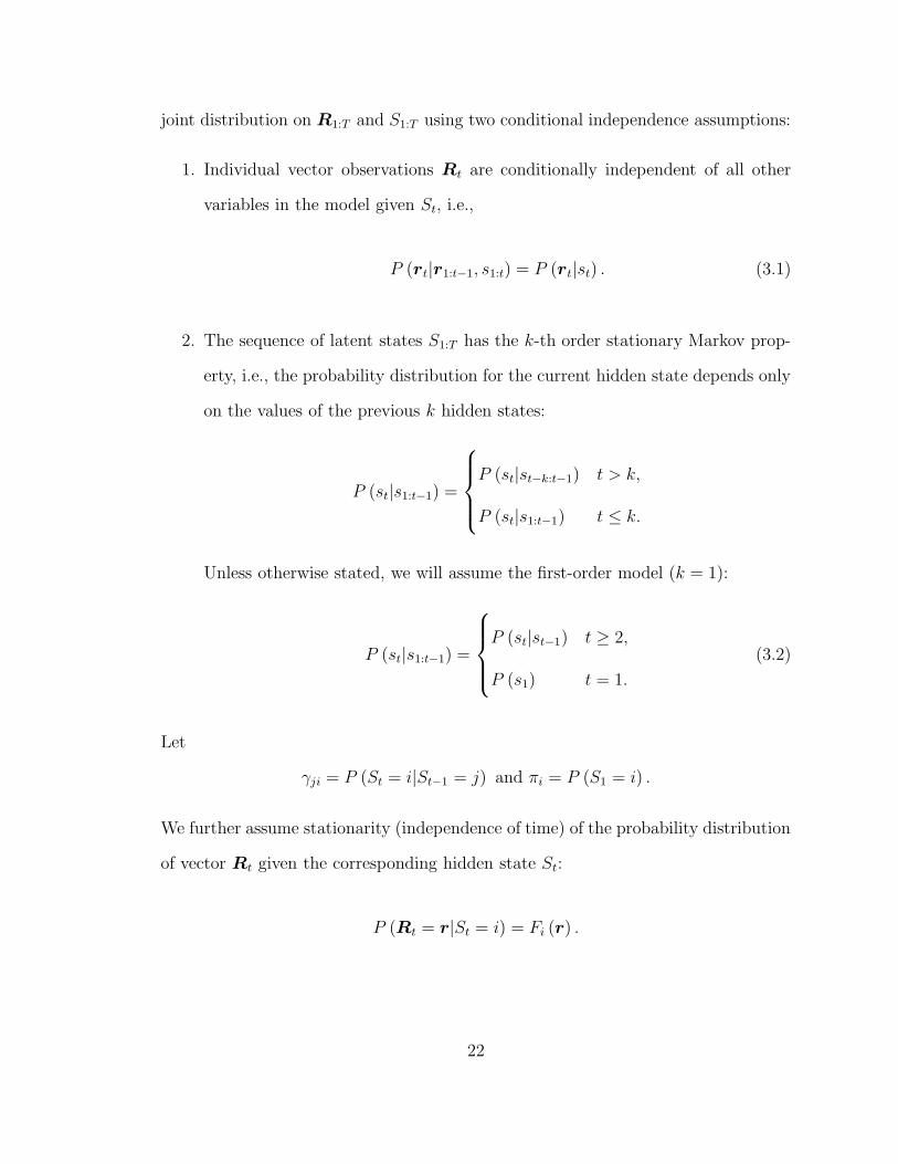
joint distribution on R1:T and S1:T using two conditional independence assumptions:

1. Individual vector observations Rt are conditionally independent of all other

variables in the model given St, i.e.,

P (rt|r1:t−1, s1:t) = P (rt|st) . (3.1)

2. The sequence of latent states S1:T has the k-th order stationary Markov prop-

erty, i.e., the probability distribution for the current hidden state depends only

on the values of the previous k hidden states:

P (st|s1:t−1) =

P (st|st−k:t−1) t > k,

P (st|s1:t−1) t ≤ k.

Unless otherwise stated, we will assume the first-order model (k = 1):

P (st|s1:t−1) =

P (st|st−1) t ≥ 2,

P (s1) t = 1.

(3.2)

Let

γji = P (St = i|St−1 = j) and πi = P (S1 = i) .

We further assume stationarity (independence of time) of the probability distribution

of vector Rt given the corresponding hidden state St:

P (Rt = r|St = i) = Fi (r) .

22

S S1 2

1 2R R

ST

TR

St

tR R

S

T−1

T−1

Figure 3.1: Bayesian network representation of a homogeneous HMM satisfying con-ditional independence assumptions (3.1) and (3.2). (Smyth et al., 1997)

The stationarity assumption for the probability P (st|st−1) defines a homogeneous

HMM; lack of stationarity for P (St|St−1) defines a non-homogeneous HMM.

For a homogeneous HMM, let Π = (π1, . . . , πK) be the first-state probability vector,

and let Γ = (γ11, . . . , γKK) be the transition matrix. Let Υ defining all of Fi (r) =

P (rt|St = i) be the set of emission parameters. The joint probability of the data

and the hidden states can then be written as

P (r1:T , S1:T = s1:T |Π,Γ,Υ) =

[

πs1

T∏

t=2

γst−1st

][

T∏

t=1

Fst(rt)

]

.

A Bayesian network representation of a homogeneous HMM is shown in Figure 3.1.

3.1.1 Auto-regressive Models

It is sometimes beneficial to represent temporal dependence in time series data not

only via the transition probability (3.2), but also by using the emission distribution.

This can be accomplished by relaxing the conditional independence assumption (3.1)

to allow direct dependence of X t on a short history of previous Xτ for τ < t. This

auto-regressive model (sometimes called a k-th order auto-regressive model) (Poritz,

1982; Rabiner, 1989) replaces the first conditional independence assumption (3.1)

23

S S1 2

1 2R R

ST

TR

St

tR R

S

T−1

T−1

Figure 3.2: Bayesian network representation of an AR-HMM satisfying conditionalindependence assumptions (3.3) and (3.2).

replaced with:

1. Individual vector observations Rt are conditionally independent of all other

variables in the model given St and the previous k observations, i.e.,

P (rt|r1:t−1, s1:t) =

P (rt|st, rt−k:t−1) t > k,

P (rt|st, r1:t−1) t ≤ k.

(3.3)

Unless otherwise specified, we consider only the first order (k = 1) auto-regressive

models.

It is trivial to observe that the original conditional independence assumption for

the emission distribution is a special case of the conditional independence assumption

for an auto-regressive model. To consider both models at the same time in the future,

we will denote P (rt|St = i, rt−1) by Fi (rt|rt−1) where for non-auto-regressive model,

Fi (rt|rt−1) = Fi (rt) = P (rt|St = i) for all values of rt−1. For auto-regressive mod-

els, Υ contains parameters for P (rt|st, rt−1), and the joint probability is expressed

as

P (r1:T , S1:T = s1:T |Π,Γ,Υ) =

[

πs1

T∏

t=2

γst−1st

][

T∏

t=1

Fst(rt|rt−1)

]

.

24

1 2R R TRtR RT−1

X X1 2 XTXt XT−1

S S1 2 STSt ST−1

Figure 3.3: Bayesian network representation of a non-homogeneous HMM satisfyingthe conditional independence assumptions (3.1) (or, seen as dashed lines, (3.3) forAR model) and (3.4).

A graphical model for a first order auto-regressive HMM (AR-HMM) is presented

in Figure 3.2. For discrete-valued R, this model is sometimes called a double-chain

Markov model (Berchtold, 1999).

3.1.2 Non-homogeneous HMMs

Sometimes the data R is known (or assumed) to be generated dependent on a set

of observed time series of variables X. For example, precipitation data can be influ-

enced by the values of atmospheric variables like sea surface pressure, wind vector,

and temperature. Homogeneous HMMs can be extended to allow the probability dis-

tribution of the output variables to be dependent on observed input variables. Here,

we adopt the non-homogeneous HMM (NHMM) framework of Hughes and Guttorp

(Hughes and Guttorp, 1994; Hughes et al., 1999). Assume that we have a sequence

of D-dimensional input column vectors X1:T = (X1, . . . ,XT ). The presence of the

input vectors replaces the (homogeneous) Markov assumption of HMMs with the

assumption that the probability for a hidden state St also depends on the value of

25

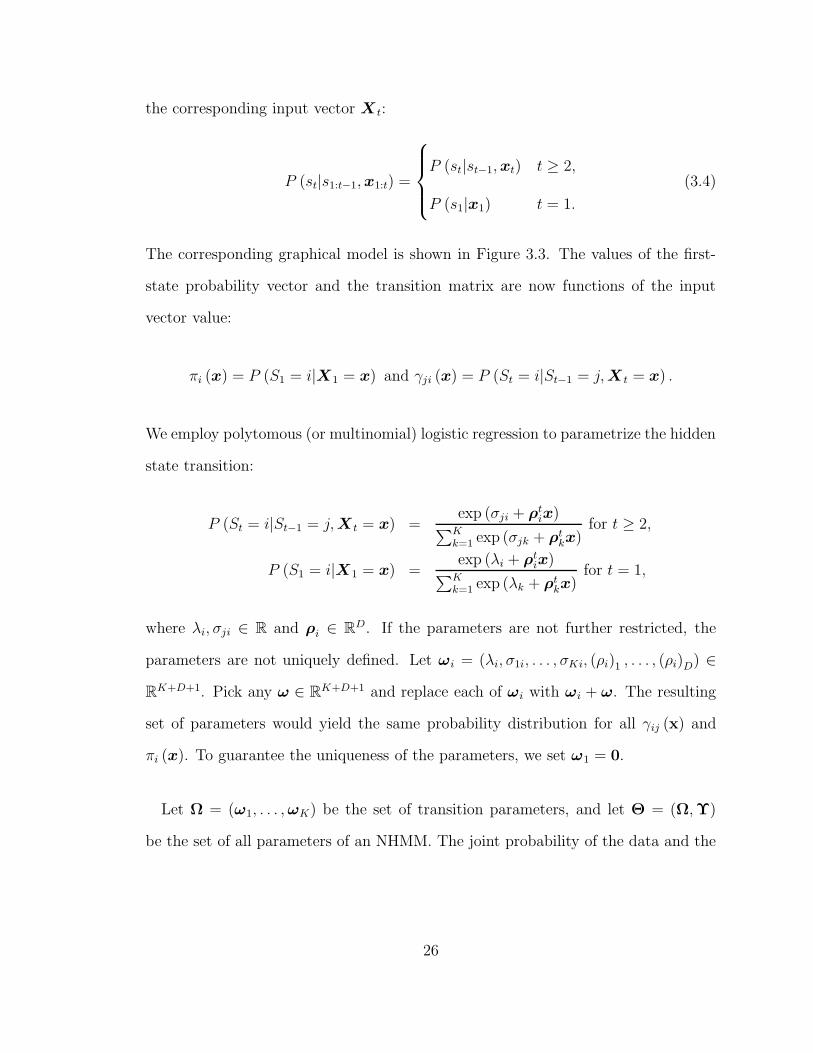
the corresponding input vector X t:

P (st|s1:t−1,x1:t) =

P (st|st−1,xt) t ≥ 2,

P (s1|x1) t = 1.

(3.4)

The corresponding graphical model is shown in Figure 3.3. The values of the first-

state probability vector and the transition matrix are now functions of the input

vector value:

πi (x) = P (S1 = i|X1 = x) and γji (x) = P (St = i|St−1 = j,X t = x) .

We employ polytomous (or multinomial) logistic regression to parametrize the hidden

state transition:

P (St = i|St−1 = j,X t = x) =exp (σji + ρt

ix)∑K

k=1 exp (σjk + ρtkx)

for t ≥ 2,

P (S1 = i|X1 = x) =exp (λi + ρt

ix)∑K

k=1 exp (λk + ρtkx)

for t = 1,

where λi, σji ∈ R and ρi ∈ RD. If the parameters are not further restricted, the

parameters are not uniquely defined. Let ωi = (λi, σ1i, . . . , σKi, (ρi)1 , . . . , (ρi)D) ∈

RK+D+1. Pick any ω ∈ R

K+D+1 and replace each of ωi with ωi + ω. The resulting

set of parameters would yield the same probability distribution for all γij (x) and

πi (x). To guarantee the uniqueness of the parameters, we set ω1 = 0.

Let Ω = (ω1, . . . ,ωK) be the set of transition parameters, and let Θ = (Ω,Υ)

be the set of all parameters of an NHMM. The joint probability of the data and the

26

hidden states can then be expressed as

P (r1:T , s1:T |x1:T ,Θ) =

[

πs1 (x1)T∏

t=2

γst−1st(xt)

][

T∏

t=1

Fst(rt|rt−1)

]

. (3.5)

Note that homogeneous HMMs are just a special case of NHMMs with

πi =exp (λi)

∑Kk=1 exp (λk)

and γji =exp (σji)

∑Kk=1 exp (σjk)

i, j = 1, . . . , K,

or, equivalently, ρi = 0, i = 1, . . . , K.

3.2 Hidden State Distributions

In this section, we assume that the set of parameters Θ is known, and we omit

dependence on Θ in all equations in this section. Given these parameters, we derive

the well-known equations and methods related to estimating the probabilities of the

unobserved states S1:T .

3.2.1 Inference

It is often desirable to calculate a probability distribution over the unobserved

variables given the observed data. In other words, we want to estimate

P (s1:T |r1:T ,x1:T ) =P (s1:T , r1:T |x1:T )

P (r1:T |x1:T )=

P (s1:T , r1:T |x1:T )∑

S1:TP (s1:T , r1:T |x1:T )

.

The numerator can be computed from Equation 3.5. The sum in the denominator,

however, has KT terms and cannot be evaluated directly. To compute the likelihood

of the data P (r1:T |x1:T ), we can employ a recursive procedure called the Forward-

Backward procedure (e.g., Rabiner, 1989). For each value of each hidden state St, we

27

recursively calculate a summary of information preceding the state (αt) and following

the state (βt) as follows:

αt (i) = P (St = i, r1:t|x1:t) and βt (i) = P (rt+1:T |St = i, rt,xt+1:T ) . (3.6)

Then

α1 (i) = P (S1 = i|x1)P (r1|S1 = i) ;

αt+1 (i) = P (rt+1|St+1 = j, rt)K∑

i=1

P (St+1 = j|St = i,xt+1)αt (i) ;

βT (i) = 1;

βt (i) =K∑

j=1

P (St+1 = j|St = i,xt+1)P (rt+1|St+1 = j, rt) βt+1 (j) .

If the computation of Fst(rt|rt−1) has time complexity O (Rtime) and storage require-

ments O (Rspace), then the time complexity of computing α’s and β’s is

O (TK (K +Rtime)) which is linear in T and quadratic in K. Space complexity

O (TK +Rspace). Using the values of α and β we can then easily evaluate the ex-

pressions needed for inference, sampling, and, later, for learning. The likelihood of

the data sequence P (R1:T |X1:T ) can be computed as

P (r1:T |x1:T ) =

K∑

i=1

P (ST = i, r1:T |x1:T ) =

K∑

i=1

αT (i) .

3.2.2 Sampling

It is sometimes necessary to sample sequences of hidden states S1:T from the posterior

distribution P (s1:T |r1:T ,x1:T ) (e.g., for Bayesian learning of the HMM parameters).

Instead of using a direct Gibbs sampler, we can use the Forward-Backward recursion

28

to sample from P (s1:T |r1:T ,x1:T ) more efficiently (Chib, 1996; Scott, 2002). First

note that

P (s1:T |r1:T ,x1:T ) =T∏

t=1

P (st|st+1:T , r1:T ,x1:T ) .

This expansion suggests the following sampling strategy: for t = T, T − 1, . . . , 1

select a sample it according to P (st|St+1:T = it+1:T , r1:T ,x1:T ). The resulting se-

quence (i1, . . . , iT ) would then be a sample from P (s1:T |r1:T ,x1:T ). To compute

P (st|st+1:T , r1:T ,x1:T ), we first notice that

P (St = i, st+1:T , r1:T |x1:T ) =

= P (St = i, r1:t|x1:t)P (st+1:T , rt+1:T |St = i, rt,xt+1:T )

= αt (i) γist+1 (xt+1)Fst+1 (rt+1|rt)P (st+2:T , rt+2:T |st+1, rt+1,xt+2:T ) . (3.7)

It follows from (3.7) that

P (St = i|st+1:T , r1:T ,x1:T ) =P (St = i, st+1:T , r1:T |x1:T )

∑Kk=1 P (St = k, st+1:T , r1:T |x1:T )

=αt (i) γist+1 (xt+1)

∑Kk=1 αt (k) γkst+1 (xt+1)

.

The time complexity of sampling is O (TK (K +Rtime)) to compute the values of

α, plus an additional O (TK) per each simulated sequence. The space complexity

is O (TK +Rspace) to compute α’s plus an additional O (T +K) per each simulated

sequence.

29

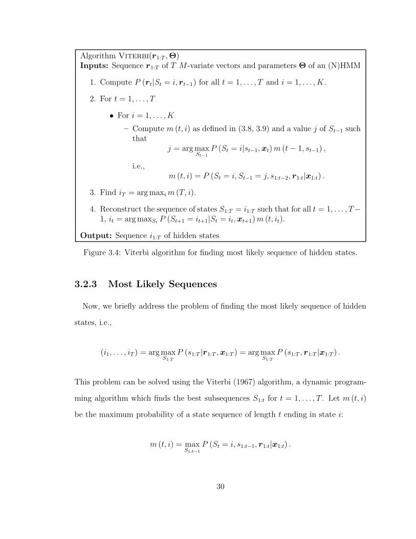
Algorithm Viterbi(r1:T ,Θ)Inputs: Sequence r1:T of T M -variate vectors and parameters Θ of an (N)HMM

1. Compute P (rt|St = i, rt−1) for all t = 1, . . . , T and i = 1, . . . , K.

2. For t = 1, . . . , T

• For i = 1, . . . , K

– Compute m (t, i) as defined in (3.8, 3.9) and a value j of St−1 suchthat

j = argmaxSt−1

P (St = i|st−1,xt)m (t− 1, st−1) ,

i.e.,m (t, i) = P (St = i, St−1 = j, s1:t−2, r1:t|x1:t) .

3. Find iT = argmaxim (T, i).

4. Reconstruct the sequence of states S1:T = i1:T such that for all t = 1, . . . , T−1, it = argmaxSt

P (St+1 = it+1|St = it,xt+1)m (t, it).

Output: Sequence i1:T of hidden states

Figure 3.4: Viterbi algorithm for finding most likely sequence of hidden states.

3.2.3 Most Likely Sequences

Now, we briefly address the problem of finding the most likely sequence of hidden

states, i.e.,

(i1, . . . , iT ) = argmaxS1:T

P (s1:T |r1:T ,x1:T ) = argmaxS1:T

P (s1:T , r1:T |x1:T ) .

This problem can be solved using the Viterbi (1967) algorithm, a dynamic program-

ming algorithm which finds the best subsequences S1:t for t = 1, . . . , T . Let m (t, i)

be the maximum probability of a state sequence of length t ending in state i:

m (t, i) = maxS1:t−1

P (St = i, s1:t−1, r1:t|x1:t) .

30

m (t, i) for t = 1, . . . , T and i = 1, . . . , K can be computed efficiently capitalizing on

the following recursive property:

m (1, i) = P (r1|S1 = i)P (S1 = i|x1) , (3.8)

m (t, i) = P (rt|St = i, rt−1)maxjP (St = i|St−1 = j,xt)m (t− 1, j) . (3.9)

This leads to the algorithm described in Figure 3.4. The algorithm has time com-

plexity of O (TK (K +Rtime)) and space complexity of O (TK +Rspace).

3.3 Learning

In this section, we review approaches for finding a set of NHMM parameters that

best fit a data set.

3.3.1 EM Framework for NHMMs

As we have seen in Section 3.1, the set of NHMM parameters Θ consists of tran-

sition parameters Ω specifying P (s1:T |x1:T ) and emission parameters Υ specifying

P (r1:T |s1:T ).

We assume the data set consists of N sequences each of length T . Let Rnt denote

the t-th data vector of sequence n, and let Xnt and Snt be the corresponding vector of

inputs and the hidden state (respectively) for the same index and sequence. Rn,1:T ,

Sn,1:T , and Xn,1:T denote n-th sequences of data, hidden states, and input vectors,

1 ≤ n ≤ N . We will also use a single symbol R, S, and X to denote all N sequences

of data, hidden states, and input vectors. We assume that the observed sequences

are conditionally independent given the model. We further assume that the data set

31

is complete, i.e., all none of the entries of R and X are missing.

In the Bayesian framework, we are interested in estimating the posterior distri-

bution of the model parameters given the data. To do so, we first assume a fixed

model structure M (for example, for NHMMs M consists of the number of hidden

states and the functional and structural form of P (r|s)), and then we define a prior

distribution P (Θ|M) on the parameters given the model. By Bayes rule

P (Θ|M,R,X) =P (Θ|X,M)P (R|X,Θ,M)

P (R|X,M).

We assume that the prior is independent of the values of the input variables.1 In

this section, we assume M is given2, and we will drop it from further equations. The

posterior distribution can then be written as

P (Θ|R,X) =P (Θ)P (R|X,Θ)

P (R|X).

Instead of looking at the full posterior, we will concentrate on finding its mode.

This maximum a posteriori approach requires finding argmaxΘ P (Θ)P (R|X,Θ).

Unless indicated otherwise, we will assume uniform priors thus utilizing the maximum

likelihood approach of finding argmaxΘ P (R|X,Θ).

1The prior certainly depends on the type of the input variables. For example, in precipitationmodeling, having X as observed sea-surface temperature and having X as observed wind vectorswould yield different priors. We assume M includes the type of X.

2The Bayesian framework allows us to define a prior on M and to study P (M|R,X).

32

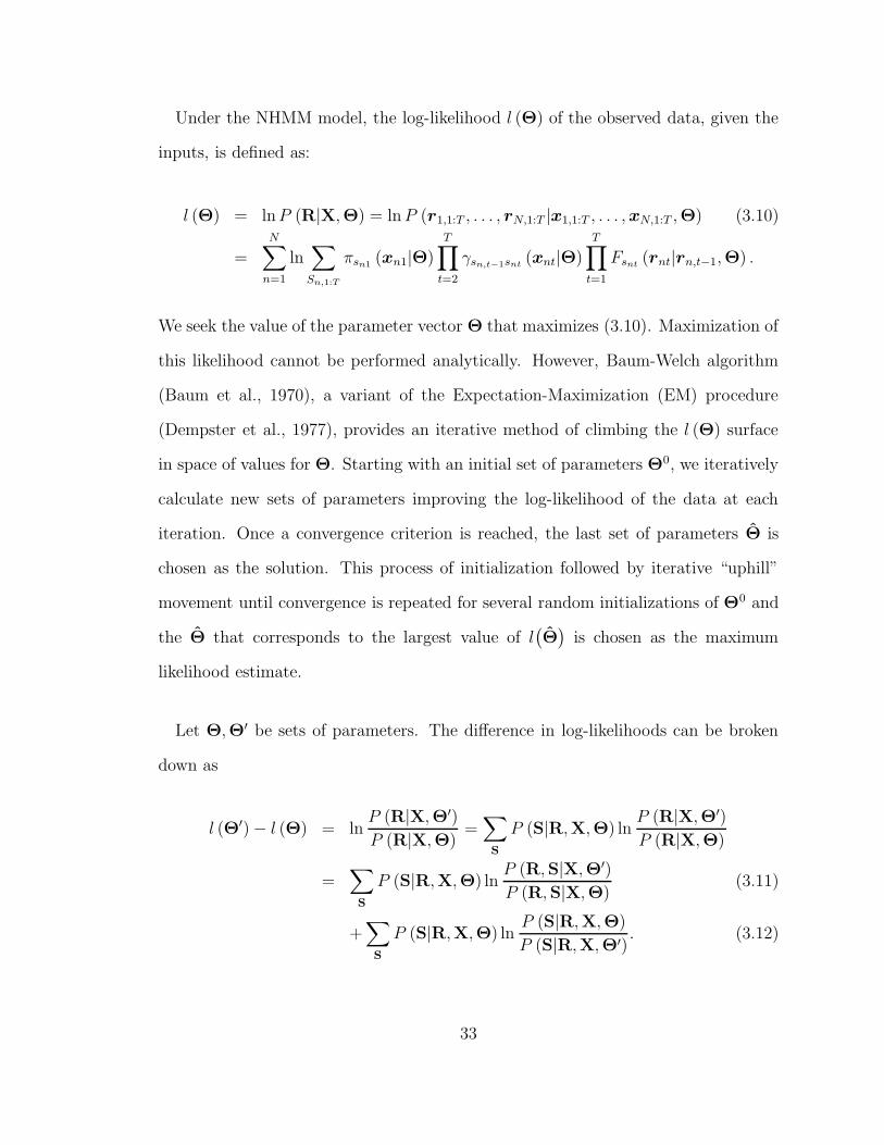
Under the NHMM model, the log-likelihood l (Θ) of the observed data, given the

inputs, is defined as:

l (Θ) = lnP (R|X,Θ) = lnP (r1,1:T , . . . , rN,1:T |x1,1:T , . . . ,xN,1:T ,Θ) (3.10)

=

N∑

n=1

ln∑

Sn,1:T

πsn1 (xn1|Θ)

T∏

t=2

γsn,t−1snt(xnt|Θ)

T∏

t=1

Fsnt(rnt|rn,t−1,Θ) .

We seek the value of the parameter vector Θ that maximizes (3.10). Maximization of

this likelihood cannot be performed analytically. However, Baum-Welch algorithm

(Baum et al., 1970), a variant of the Expectation-Maximization (EM) procedure

(Dempster et al., 1977), provides an iterative method of climbing the l (Θ) surface

in space of values for Θ. Starting with an initial set of parameters Θ0, we iteratively

calculate new sets of parameters improving the log-likelihood of the data at each

iteration. Once a convergence criterion is reached, the last set of parameters Θ is

chosen as the solution. This process of initialization followed by iterative “uphill”

movement until convergence is repeated for several random initializations of Θ0 and

the Θ that corresponds to the largest value of l(

Θ)

is chosen as the maximum

likelihood estimate.

Let Θ,Θ′ be sets of parameters. The difference in log-likelihoods can be broken

down as

l (Θ′) − l (Θ) = lnP (R|X,Θ′)

P (R|X,Θ)=∑

S

P (S|R,X,Θ) lnP (R|X,Θ′)

P (R|X,Θ)

=∑

S

P (S|R,X,Θ) lnP (R,S|X,Θ′)

P (R,S|X,Θ)(3.11)

+∑

S

P (S|R,X,Θ) lnP (S|R,X,Θ)

P (S|R,X,Θ′). (3.12)

33

Expression 3.12 is a relative entropy (or Kullback-Leibler divergence) between

P (S|R,X,Θ) and P (S|R,X,Θ′). Given two distributions p (x) and q (x) on x ∈ X ,

the KL-divergence is defined as

KL (p ‖ q) =∑

x

p (x) lnp (x)

q (x).

KL can be thought of as an asymmetric distance between the distributions since

KL (p ‖ q) ≥ 0 with KL (p ‖ q) = 0 if and only if p ≡ q, and in general, KL (p ‖ q) 6=

KL (q ‖ p). (For more information on the KL-divergence, refer to Cover and Thomas

(1991)). Since (3.12) is non-negative,

l (Θ′) − l (Θ) ≥∑

S

P (S|R,X,Θ) lnP (R,S|X,Θ′)

P (R,S|X,Θ)

=∑

S

P (S|R,X,Θ) lnP (R,S|X,Θ′) −∑

S

P (S|R,X,Θ) lnP (R,S|X,Θ) .

To update the parameters Θr+1 at iteration r, we maximize

Q(

Θr,Θr+1)

= EP (S|R,X,Θr)

[

lnP(

S,R|X,Θr+1)]

= (3.13)

=

N∑

n=1

∑

Sn,1:T

P (sn,1:T |rn,1:T ,xn,1:T ,Θr) lnP

(

sn,1:T , rn,1:T |xn,1:T ,Θr+1)

.

By (3.13), l (Θr+1) − l (Θr) ≥ Q (Θr,Θr+1) − Q (Θr,Θr), so by maximizing

Q (Θr,Θr+1), we guarantee that the log-likelihood will not decrease.

Q (Θr,Θr+1) is maximized in two steps. In the first, the E-step, we calculate

P (sn,1:T |rn,1:T ,xn,1:T ,Θr). In the second, the M-step, we maximize Q (Θr,Θr+1)

with respect to the parameters in Θr+1. It is clearly infeasible to compute and store

probabilities of N×KT possible sequences of hidden states P (sn,1:T |rn,1:T ,xn,1:T ,Θr)

34

as suggested in the E-step. It turns out that only a manageable set of N × T × K

probabilities Ant (i) = P (Snt = i|rn,1:T ,xn,1:T ,Θr) andN×(T − 1)×K2 probabilities

Bnt (i, j) = P (Snt = i, Sn,t−1 = j|rn,1:T ,xn,1:T ,Θr) are needed to perform optimiza-

tion in the M-step:

Q(

Θr,Θr+1)

=N∑

n=1

∑

Sn,1:T

P (sn,1:T |rn,1:T ,xn,1:T ,Θr) lnP

(

sn,1:T , rn,1:T |xn,1:T ,Θr+1)

=N∑

n=1

∑

Sn,1:T

P (sn,1:T |rn,1:T ,xn,1:T ,Θr) ×

(

T∑

t=1

lnP(

rnt|snt, rn,t−1,Θr+1)

+ lnP(

sn1|xn1,Θr+1)

+

T∑

t=2

lnP(

snt|sn,t−1,xnt,Θr+1)

)

=N∑

n=1

T∑

t=1

K∑

i=1

Ant (i) lnP(

rnt|Snt = i, rn,t−1,Θr+1)

(3.14)

+

N∑

n=1

K∑

i=1

An1 (i) lnP(

Sn1 = i|xn1,Θr+1)

(3.15)

+N∑

n=1

T∑

t=2

K∑

i=1

K∑

j=1

Bnt (i, j) lnP(

Snt = i|Sn,t−1 = j,xnt,Θr+1)

. (3.16)

The quantities Ant and Bnt can be calculated using values of α and β (3.6) for

sequence n as computed by the recursive Forward-Backward procedure:

Ant (i) =αnt (i) βnt (i)∑K

k=1 αnT (k)and Bnt (i, j) =

Fi (rnt|rn,t−1) γji (xnt)αn,t−1 (j)βnt (i)∑K

k=1 αnT (k).

For the M-step, we find a set of parameters Θr+1 maximizing Q (Θr,Θr+1) (with

added Lagrangians to adjust for constraints). It helps to notice first that the Expres-

sion 3.14 (we will denote it QR (Υr+1)) and expressions 3.15 and 3.16 (we will denote

their sum QS (Ωr+1)) can be optimized independently of each other. We discuss the

35

optimization of QR with respect to various emission distributions with parameters

Υr+1 in Section 3.4. For the homogeneous case, the updated parameters can be

computed in closed form by solving a system of equations obtained by setting to zero

partial derivatives of QS (Ωr+1) (with added Lagrangians to adjust for constraints)

with respect to parameters of Γ and Π:

π(r+1)i =

∑Nn=1An1 (i)

Nand γ

(r+1)ji =

∑Nn=1

∑Tt=2Bnt (i, j)

∑Nn=1

∑T−1t=1 Ant (j)

.

Unfortunately, in the non-homogeneous case, the parameters of the transition

P (St|St−1,X t) have non-linear partial derivatives, and the system of equations re-

sulting from equating their partial derivatives to zero cannot be solved analytically.

We use a conjugate gradient algorithm to find a set of parameters Ωr+1 making

QS (Ωr+1) ≥ 0. The details are provided in Appendix A.1.

3.4 Modeling Emission Distributions

As was seen earlier in the chapter, the M-step for finding the parameters in an

HMM can be split into maximization with respect to the transition parameters and

maximization with respect to emission parameters, i.e., the optimization of

QR

(

Υr+1)

=

N∑

n=1

T∑

t=1

K∑

i=1

Ant (i) logP(

rnt|Snt = i, rn,t−1,Υr+1)

(3.17)

where Ant (i) = P (Snt = i|rn,1:T ,xn,1:T ,Θr). An intuitive way to interpret this op-

timization problem is to view it as approximating K probability distributions with

weighted or fractional data samples where for a distribution i a data point Rnt has

weight Ant (i). The specifics of the optimization depend on the forms of distribution

for each of the hidden states P (r|S = i, rprevious,Υ), i = 1, . . . , K.

36

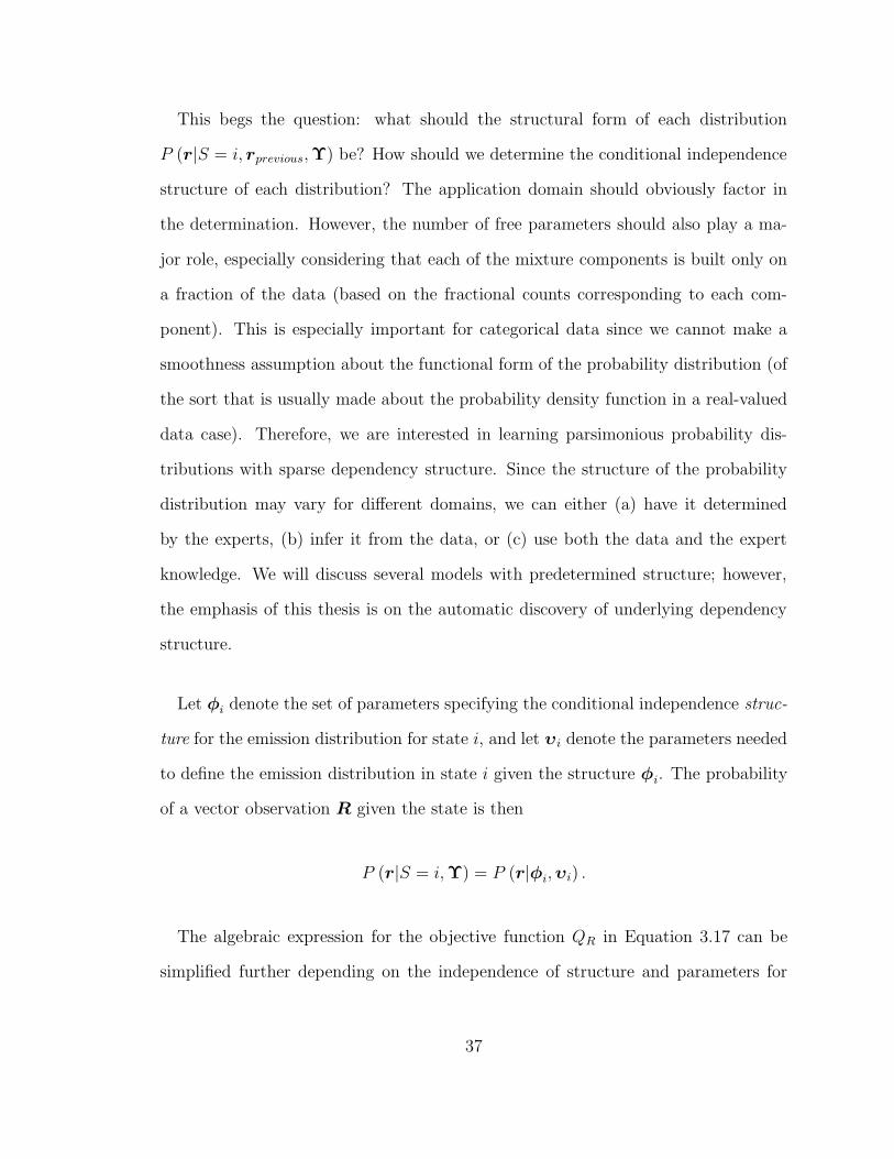
This begs the question: what should the structural form of each distribution

P (r|S = i, rprevious,Υ) be? How should we determine the conditional independence

structure of each distribution? The application domain should obviously factor in

the determination. However, the number of free parameters should also play a ma-

jor role, especially considering that each of the mixture components is built only on

a fraction of the data (based on the fractional counts corresponding to each com-

ponent). This is especially important for categorical data since we cannot make a

smoothness assumption about the functional form of the probability distribution (of

the sort that is usually made about the probability density function in a real-valued

data case). Therefore, we are interested in learning parsimonious probability dis-

tributions with sparse dependency structure. Since the structure of the probability

distribution may vary for different domains, we can either (a) have it determined

by the experts, (b) infer it from the data, or (c) use both the data and the expert

knowledge. We will discuss several models with predetermined structure; however,

the emphasis of this thesis is on the automatic discovery of underlying dependency

structure.

Let φi denote the set of parameters specifying the conditional independence struc-

ture for the emission distribution for state i, and let υi denote the parameters needed

to define the emission distribution in state i given the structure φi. The probability

of a vector observation R given the state is then

P (r|S = i,Υ) = P (r|φi,υi) .

The algebraic expression for the objective function QR in Equation 3.17 can be

simplified further depending on the independence of structure and parameters for

37

different states. Commonly, the emission parameters νi for different states i are

assumed to be independent of each other, and in this thesis we make this assumption

as well. (Kirshner et al. (2003) describe an example of a mixture model with shared

parameters.) We can further assume that the structures φi of emission distributions

for different states i are also independent. Then the objective function QR can be

rewritten as

QR

(

Υr+1)

=

N∑

n=1

T∑

t=1

K∑

i=1

Ant (i) logP(

rnt|φr+1i ,υr+1

i

)

=K∑

i=1

(

N∑

ν=1

T∑

τ=1

Aντ (i)

)

N∑

n=1

T∑

t=1

Ant (i)∑N

ν=1

∑Tτ=1Aντ (i)

logP(

rnt|φr+1i ,υr+1

i

)

=

K∑

i=1

Ci

N∑

n=1

T∑

t=1

Wnt (i) logP(

rnt|φr+1i ,υr+1

i

)

(3.18)

where Ci =∑N

n=1

∑Tt=1Ant (i) and Wnt (i) = Ant(i)

Ci. Note that

N∑

n=1

T∑

t=1

Wnt (i) =

N∑

n=1

T∑

t=1

Ant (i)

Ci=

N∑

n=1

T∑

t=1

Ant (i)∑N

ν=1

∑Tτ=1Aντ (i)

= 1.

By setting

Pi (r) =

N,T∑

n=1,t=1

Rnt=r

Wnt (i) , (3.19)

we define a probability distribution Pi (r) on R. The objective function can then be

rewritten as

QR

(

Υr+1)

=

K∑

i=1

Ci

N∑

n=1

T∑

t=1

Wnt (i) logP(

rnt|φr+1i ,υr+1

i

)

=K∑

i=1

Ci

∑

r∈R

Pi (r) logP(

r|φr+1i ,υr+1

i

)

,

38

and can be optimized by independently finding φr+1i and υr+1

i to maximize∑

r∈R Pi (r) logP(

r|φr+1i ,υr+1

i

)

. This is equivalent to minimizing

KL(

Pi ‖ P(

·|φr+1i ,υr+1

i

))

independently for each i = 1, . . . , K. Both of these op-

timization problems are usually solved by finding zeros of partial derivatives with

respect to the parameters (while checking that the resulting value of the objective

function is a maximum). Chapters 4 and 5 deal with various categorical and real-

valued distributions which can be used to model P (r|S = i,υi).

If the distributions in each hidden state share an unknown conditional indepen-

dence structure φ, QR in the form (3.18) cannot be optimized independently for

different i. (Examples of such models can be found in Meila and Jordan (2000) and

Bilmes (1999).) However, note that

K∑

i=1

Ci =K∑

i=1

N∑

n=1

T∑

t=1

Ant (i) =N∑

n=1

T∑

t=1

(

K∑

i=1

P (Snt = i|rn,1:T ,xn,1:T ,Θr)

)

= NT.

We can recast QR as

QR

(

Υr+1)

=

N∑

n=1

T∑

t=1

K∑

i=1

Ant (i) logP(

rnt|φr+1,υr+1i

)

=K∑

i=1

Ci

N∑

n=1

T∑

t=1

Wnt (i) logP(

rnt|φr+1,υr+1i

)

= NT

K∑

i=1

PS (i)∑

r∈R

Pi (r) logP(

r|φr+1,υr+1i

)

with PS (i) = Ci

NTdefining a distribution over hidden states i = 1, . . . , K. Thus

maximizing QR (Υr+1) is equivalent to minimizing the conditional relative entropy

39

KLΥr+1|S (Pi|P ):

KLΥr+1|S

(

Pi ‖ P(

·|Υr+1))

=

K∑

i=1

PS (i)∑

r∈R

Pi (r) logPi (r)

P(

r|φr+1,υr+1i

) .

The conditional relative entropy has the same property as the relative entropy (also

called Kullback-Leibler divergence):

KL (p (x|y) ‖ q (x|y)) =∑

y

p (y)∑

x

p (x|y) logp (x|y)q (x|y) ≥ 0

with KL (p (x|y) ‖ q (x|y)) = 0 iff p (x|y) ≡ q (x|y).

3.5 Historical Remarks and Connections to Other

Models

Hidden Markov models were known and used for speech processing as early as

1960’s (Baum and Petrie, 1966). While initially mostly used in speech commu-

nity, HMMs and their variations were also found to be useful in other applications,

e.g., biology and bioinformatics (e.g., Krogh et al., 1994; Baldi and Brunak, 2001),

economics (e.g., Bhar and Hamori, 2004), vision task recognition (e.g., Brand et al.,

1997), music segmentation (e.g., Raphael, 1999), freeway traffic modelling (e.g., Kwon

and Murphy, 2000), and the application considered in this thesis, multi-site precip-

itation occurrence modeling (e.g., Hughes and Guttorp, 1994; Hughes et al., 1999).

Non-homogeneous HMMs were first introduced by Hughes and Guttorp (1994) to

model multi-station rainfall occurrences for Washington state. Independently, and

at roughly the same time, Bengio and Frasconi (1995) proposed an Input/Output

HMM (IOHMM) framework allowing not only non-stationary transitions between

40

hidden states, but also modeling output vectors dependent on both hidden states

and input variables. Meila and Jordan (1996) also proposed a type of NHMM as an

extension of the mixture of experts.

There are several well-studied models related to NHMMs. If we make the tran-

sition matrix of a non-AR model to have all rows identical, we arrive at a (non-

homogeneous) mixture model (or a mixture of experts (Jordan and Jacobs, 1994))

without the dependence on time t:

P (St = i|xt) = πi (xt) and P (rt|xt) =

K∑

i=1

πi (xt)Fi (rt) ∀t = 1, . . . , T.

By considering a degenerate case of K = 1 for an AR-HMM, we obtain a first-order

auto-regressive model of the vector series R1:T :

P (r1:T ) = P (r1:T )

T∏

t=2

P (rt|rt−1) .

NHMMs can also be viewed as both a special case of a more general class of

temporal models called dynamic Bayesian networks (DBNs) (e.g., Murphy, 2002).

DBNs define a probability distribution over a time-dependent set of variables. Just

as with NHMMs, the variables or vectors can be broken into three types: R, observed

data (or output) vectors or sets of variables, S, vector or a set of latent or hidden

variables, and X, a set of input data vectors. The joint distribution is based on one

conditional independence assumption, Markov dependency of the consecutive time

slices:

P (rt, st|r1:t−1, s1:t−1,x1:T ) =

P (rt, st|rt−1, st−1,xt) t > 1

P (r1, s1|x1) t = 1.

(3.20)

41

with conditional independencies of probability distributions in both cases of (3.20)

represented by Bayesian networks. Our formulation of NHMMs also allows

P (rt, st|xt) to have a graphical model representation dependent on the value of

St, something standard DBNs do not allow. This can be corrected by representing

P (rt, st|xt) by a Bayesian multinet (Geiger and Heckerman, 1996), a set of Bayesian

nets for different values of some of the variables. (When the structure of the Bayesian

nets differs according to the value of a latent variable (the scenario we consider in the

previous section), the problem is usually treated as a mixture of Bayesian networks or

DAGs (Thiesson et al., 1999).) By combining temporal Bayesian structure of DBNs

with flexibility of multinets, we obtain dynamic Bayesian multinets (Bilmes, 2000).

3.6 Summary

We have defined the NHMM in this chapter and showed how to perform inference

and to learn the parameters of such a model. All of the results in this chapter

are known in the literature with the exception of conjugate gradient method for

learning NHMMs. In the next two chapters we will focus on modeling multivariate

distributions for the emission distribution component of HMMs and NHMMs.

42

Chapter 4

Parsimonious Models for

Multivariate Distributions for

Categorical Data

In this chapter, we discuss modeling joint distributions for vectors of categorical

(finite-valued) data. These models vary in the complexity of their dependence struc-

tures, and we are particularly interested in using them as emission distributions with

HMMs. In the remainder of this chapter, however, we will focus on multivariate

structure and not explicitly refer to the HMM context (models discussed here will

be integrated with HMMs in Chapter 6). Our contributions in this chapter relate

to learning multivariate joint and conditional distributions without a predefined de-

pendence structure. For these models, we will learn both the parameters and the

dependence structure.

43

As in Chapter 2.2, suppose that a multivariate distribution P (x) is defined on

domain X = X1 × · · · × XM .1 By finite-valued, nominal-valued, or categorical we

mean a distribution defined on a finite-valued domain, i.e., |X | <∞. We denote the

number of domain values for each of the variables by Bm = |Xm| <∞, m = 1, . . . ,M .

We further assume that Xm = 0, 1, . . . , Bm − 1. For simplicity, we assume that all

of the variables have the same cardinality B = B1 = · · · = BM . All of the results in

this chapter can be trivially extended to domains of unequal cardinality.

We will also consider modeling conditional probability distributions P (x|y) where

Y is a My-dimensional finite valued vector random variable with domain Y = Y1 ×

. . .YMy. Let Vy be a set of vertices corresponding to variables of Y with |Vy| = My.

We further assume that all of variables of Y have the same domain cardinality B

as variables of X. While some of the conditional distributions discussed in this

section can be applied to general finite valued Y , we will pay special attention to

distributions where the conditioning variable Y is defined on the same domain as X,

i.e., X = Y. We intend to use these distributions to model auto-regressive emission

distributions with HMMs.

Unless otherwise constrained, an M -variate joint probability distribution with each

variable taking onB values requires BM−1 free parameters to specify it. This number

of parameters is intractable to work with even for relatively small values of B and

M due to, among other reasons, insufficient data to learn the parameters of the

distribution accurately. One way to limit the number of free parameters is to restrict

the dependency structure of the distribution. As a result, we may not be able to

capture the multivariate dependencies involving large number of variables. However,

we are often interested primarily in capturing local or low-order (e.g., second-order or

1The notation is overloaded as random variable X is not the same as input vector in Chapter 3

44

pairwise) dependencies. By considering distributions expressible in the form of low-

order distributions, we can drastically reduce the dimensionality of the parameter

space. A distribution modeling only l-variable blocks of the M -variate distribution

will require O((

Ml

)

Bl)

free parameters, manageable for small values of l, as compared

to O(

BM)

free parameters required by an unconstrained distribution. Moreover, we

are often interested in even sparser structures, i.e., where only a small number of

l-variable interactions would be modeled directly, with the rest of the interactions

either modeled indirectly (through interactions with other variables) or by lower order

blocks of variables. For example, a model encoding only univariate and bivariate

variable interactions for M -variate binary data will require only M (M + 1) /2 free

parameters2 as compared to 2M − 1 free parameters needed to define an arbitrary

distribution on an M -variate binary vector. For the case of conditional distributions,

the number of free parameters is even larger since interactions of variables of X

are also dependent on variables Y . Sometimes the number of free parameters can

be reduced by adding unobserved variables (e.g., mixture models); however, this

significantly complicates learning of the structure, and sometimes, of the parameters.

Abstractly, in a maximum likelihood context, we can consider the problem of

approximating a target distribution P (x), where P (x) is usually not defined in a

parametric form but rather empirically, as a set D =

x1, . . . ,xN

of M -dimensional

vectors, possibly with a positive weight assigned to each vector. For example, in the

context of HMMs, the parameter update for emission distribution for state i has

target distribution Pi (r) composed of data points R with corresponding weights

A (i) = Ant (i)n=1,...,N, t=1,...,T . For simplicity, we assume everywhere in this chap-

ter that D is complete, meaning that all M components are observed for all N vectors

2We will see an example of such distribution in Section 4.3.

45

in the set. While we discuss some of more general models, we concentrate on the

models directly capturing only the first- and second-order (univariate and bivariate)

interactions (l = 2). First we consider the simplest model assuming independence of

variables (l = 1) and a simple extension of it to a conditional model (Section 4.1).

The independence model has low time complexity for all operations, and thus is very

practical. After that, we consider second order models of intermediate time com-

plexities. Among them, we consider tree-structured models in Section 4.2 (including

a novel model for conditional distributions, Section 4.2.1) which can be learned with

high efficiency. Then, in Section 4.3 we consider more general exponential mod-

els based on the maximum entropy principle allowing a broad class of conditional

independencies. We also introduce a new factored probability model with factors

expressed in the form of conditional maximum entropy models (Section 4.3.2) and

describe algorithms for estimating both the parameters and the structure. Finally, a

few alternative models are considered in Section 4.4.

4.1 Independence and Conditional Independence

Models

The independence model3 decomposes the joint probability distribution on vari-

ables X = (X1, . . . , XM) into the product of marginal probabilities of individual

variables:

PI (x) =

M∏

m=1

PI (xm) .

3Note: implicit in our discussion is the fact that we are building a model for each state in theHMM. So what is called an “independence model” here is in reality a conditional independencemodel given states.

46

In order to specify the distribution under the independence model, we need to

specify the parameters for each of P (xm). Since each of Xm takes on B values, let

pmb = PI (Xm = b) , b = 0, . . . , B− 1. For each m = 1, . . . ,M,∑B−1

b=0 pmb = 1, so we

need B − 1 free parameters for each PI (xm), and M (B − 1) free parameters total.

Next, we address the parameter estimation. Let

υ = pmbm=1,...,M, b=0,...,B−1 .

Given a distribution P (x) defined on R, we want to find υ to minimize

KL (P ‖ PI (·|υ)):

argminυ

KL (P ‖ PI (·|υ)) = argminυ

∑

X

P (x) logP (x)

∏Mm=1 PI (xm|υ)

=

=M∑

m=1

arg minpm0,...,pm,B−1

KL (P (xm) ‖ PI (xm|pm0, . . . , pm,B−1)) ,

so the parameters for pm0, . . . , pm,B−1 can be estimated independently of other m.

The minimum of KL is reached when the distributions are identical, i.e.,

pmb = P (Xm = b) ∀m = 1, . . . ,M, b = 0, . . . , B − 1. (4.1)

4.1.1 Auto-regressive Conditional Independence

The independence model can be trivially extended to a conditional model given

Y by assuming that individual variables Xm are conditionally independent given Y

(Figure 4.1, left):

PCI (x|y) =M∏

m=1

PCI (xm|y) .

47

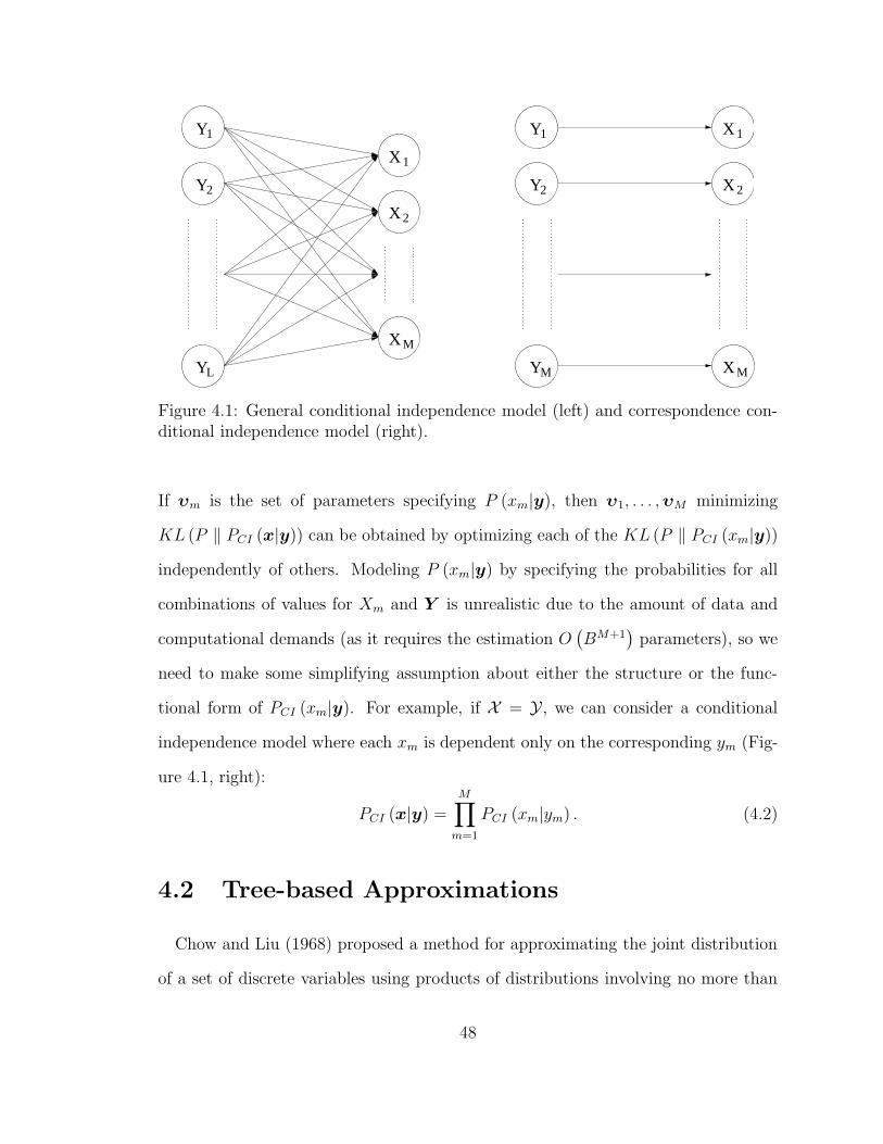
Y

Y

Y

2

1

2

L

1

MX

X

X

Y

Y

Y

2

1

M

1X

2X

MX

Figure 4.1: General conditional independence model (left) and correspondence con-ditional independence model (right).

If υm is the set of parameters specifying P (xm|y), then υ1, . . . ,υM minimizing

KL (P ‖ PCI (x|y)) can be obtained by optimizing each of the KL (P ‖ PCI (xm|y))

independently of others. Modeling P (xm|y) by specifying the probabilities for all

combinations of values for Xm and Y is unrealistic due to the amount of data and

computational demands (as it requires the estimation O(

BM+1)

parameters), so we

need to make some simplifying assumption about either the structure or the func-

tional form of PCI (xm|y). For example, if X = Y, we can consider a conditional

independence model where each xm is dependent only on the corresponding ym (Fig-

ure 4.1, right):

PCI (x|y) =

M∏

m=1

PCI (xm|ym) . (4.2)

4.2 Tree-based Approximations

Chow and Liu (1968) proposed a method for approximating the joint distribution

of a set of discrete variables using products of distributions involving no more than

48

pairs of variables. If P (x) is an M -variate distribution on discrete variables and

V = v1, . . . , vM is a set of nodes corresponding to variables in X , the Chow-Liu

method constructs a distribution T (x) for which the corresponding Bayesian and

Markov network is tree-structured. If GT = (V, ET ) is the Markov network associated

with T , then

T (x) =

∏

u,v∈ETT (xu, xv)

∏

v∈V T (xv)degree(v)

=∏

u,v∈ET

T (xu, xv)

T (xv)T (xu)

∏

v∈V

T (xv) . (4.3)

Chow and Liu showed that in order to minimize KL (P ‖ T ), the edges for the tree

ET have to be selected to maximize the total mutual information∑

u,v∈ETI (xu, xv)

of the edges. Mutual information between variables xu and xv is defined as

I (xu, xv) =∑

Xu

∑

Xv

P (xu, xv) lnP (xu, xv)

P (xu)P (xv). (4.4)

The optimal tree can be found by calculating mutual information I (xu, xv) for all

possible pairs of variables in V, and then solving the maximum spanning tree problem,

with pairwise mutual information from Equation 4.4 as edge weights (e.g., Cormen

et al., 1990). Once the edges are selected, the probability distribution T on the pairs

of vertices connected by edges is defined to be the same as in the target distribution

P :

∀ u, v ∈ ET T (xu, xv) = P (xu, xv) , (4.5)

and the resulting distribution T minimizes KL (P ‖ T ). Figure 4.2 outlines the

algorithm for finding T .

The proof that T is indeed the tree-structured distribution closest to P consists

of two parts. First, for any given tree structure for T , to minimize KL (P ‖ T ),

49

Algorithm ChowLiu(P )Inputs: Distribution P over domain X ; procedure MWST( weights ) that outputsa maximum weight spanning tree over V

1. Compute marginal distributions P (xu, xv) and P (xu) ∀u, v ∈ V

2. Compute mutual information values I (xu, xv) ∀u, v ∈ V

3. ET = MWST (I (xu, xv))

4. Set T (xu, xv) = P (xu, xv) ∀ u, v ∈ ET

Output: T

Figure 4.2: Chow-Liu algorithm (very similar to Meila and Jordan, 2000).

P ≡ T on all pairwise distributions corresponding to an edge in the graph and on all

univariate marginals, so the optimal T must satisfy the property in (4.5). (This will

be shown later, in Corollary 4.3.) For a tree-structured T satisfying (4.5),

KL (P ‖ T ) =∑

X

P (x) lnP (x)

T (x)

= −HP [X] −∑

X

P (x)

∑

v∈V

T (xv) +∑

u,v∈ET

T (xu, xv)

T (xu)T (xv)

= −HP [X] −∑

v∈V

∑

Xv

P (xv) lnP (xv) −∑

u,v∈ET

∑

Xu,Xv

P (xu, xv) lnP (xu, xv)

P (xu)P (xv)

= −HP [X] +∑

v∈V

HP [Xv] −∑

u,v∈ET

I (xu, xv) .

Since entropies HP are independent of the structure of GT , the minimum of

KL (P ‖ T ) corresponds to the structure maximizing∑

u,v∈ETI (xu, xv).

If each of the variables in V takes on B values, finding the optimal tree T has

time complexity O (M 2B2) for the mutual information calculations and O (M 2) for

finding the maximum spanning tree, totalling O (M 2B2). (For the case of sparse

50

high-dimensional data, Meila (1999) showed that the Chow-Liu algorithm can be

sped up.)

The advantages of Chow-Liu trees include (a) the existence of a simple algorithm

for finding the optimal tree 4, (b) the parsimonious nature of the model (the number

of parameters is linear in dimensionality of the space), and (c) the resulting tree

structure T often has a simple intuitive interpretation. While there are other algo-

rithms that retain the idea of a tree-structured distribution, while allowing for more

complex dependencies (e.g., thin junction trees, Bach and Jordan, 2002), these al-

gorithms have higher time complexity than the original Chow-Liu algorithm and do

not guarantee optimality of the structure that is learned. Thus, in the results in this

paper we focus on Chow-Liu trees under the assumption that they are a generally

useful modeling technique in the context of multivariate data.

4.2.1 Conditional Chow-Liu Forests

We now propose an extension of the Chow-Liu method to model conditional distri-

butions (Kirshner et al., 2004). The trivial extension of building a Chow-Liu tree for

each value of the conditioning variable Y is computationally impractical due to the

exponential (in M) number of free parameters. As with Chow-Liu trees, we want the

corresponding probability distribution to be factored into a product of distributions

involving no more than two variables. Pairs of variables are represented as an edge

in a corresponding graph with nodes corresponding to variables in Vxy = V ∪ Vy.

However, since all of the variables in Vy are observed, we are not interested in mod-

eling P (y), and do not wish to restrict P (y) by making independence assumptions

4In fact, if we change the structure to allow cliques of size more than 2 in the graph GT , theproblem of finding optimal approximation distribution becomes NP-hard (Chickering, 1996; Srebro,2003).

51

Algorithm CondChowLiu(P )Inputs: Distribution P over domain X × Y; procedure MWST( Vxy, weights )that outputs a maximum weight spanning tree over Vxy

1. (a) Compute marginal distributions P (xu, xv) and P (xu) ∀u, v ∈ V(b) Compute marginal distributions P (yu) and P (yu, xv) ∀u ∈ Vy,

v ∈ V

2. (a) Compute mutual information values I (xu, xv) ∀u, v ∈ V(b) Compute mutual information values I (yu, xv) ∀u ∈ Vy, v ∈ V(c) Find u (v) = argmaxu∈Vy

I (yu, xv) ∀v ∈ V(d) Let V ′ = V ∪ v′, and set I (xv′ , xv) = I

(

yu(v), xv

)

∀v ∈ V

3. (a) ET ′ = MWST (V ′, I)

(b) Ex = u, v |u, v ∈ V, u, v ∈ ET ′(c) Ey = u (v) , v |v ∈ V, v, v′ ∈ ET ′.

4. (a) Set T (xu, xv) = P (xu, xv) ∀ u, v ∈ Ex

(b) Set T (yu, xv) = P (yu, xv) ∀ u, v ∈ Ey

Output: T

Figure 4.3: Conditional Chow-Liu algorithm (Kirshner et al., 2004).

about the variables in Vy.5 The structure for an approximation distribution T (x|y)

will be constructed by adding edges such as not to introduce paths involving multi-

ple variables from Vy. T can be trivially extended to a joint distribution by setting

T (y) ≡ P (y).

Let GF = (Vxy, EF ) be an undirected forest, a collection of disjoint trees, containing

edges Ex between pairs of variables in V and edges Ey connecting variables in V and

Vy, EF = Ex ∪ Ey. If the probability distribution T (x|y) has forest GF for a Markov

5The graphical model structure not making any conditional independence assumptions is thecomplete graph; we may assume that the nodes in Vy form a clique.

52

network, then similar to Equation 4.3:

T (x|y) =∏

u,v∈Ex

T (xu, xv)

T (xu)T (xv)

∏

v∈V

T (xv)∏

u,v∈Ey

T (yu, xv)

T (yu)T (xv)(4.6)

=∏

u,v∈Ex

T (xu, xv)

T (xu)T (xv)

∏

v∈V

T (xv)∏

u,v∈Ey

T (xv|yu)

T (xv).

We will again use the KL-divergence, this time between conditional distributions

P (x|y) and T (x|y), as an objective function:

KL (P ‖ T ) =∑

Y

P (y)∑

X

P (x|y) lnP (x|y)

T (x|y).

It can be shown that the optimal probability distribution T with corresponding

Markov network GF is

T (xu, xv) = P (xu, xv) ∀ u, v ∈ Ex, (4.7)

and

T (xv|yu) = P (xv|yu) ∀ u, v ∈ Ey. (4.8)

As with the unconditional distribution, we wish to find pairs of variables to minimize

KL (P ‖ T ) =∑

v∈Vx

HP [Xv]−HP [X|Y ]−∑

u,v∈Ex

I (xu, xv)−∑

u,v∈Ey

I (yu, xv) (4.9)

where HP [Xv] denotes the entropy of P (xv), and HP [X|Y ] denotes the conditional

entropy of P (x|y). Both HP [Xv] and HP [X|Y ] are independent of EF , so as in

the unconditional case, we need to solve a maximum spanning tree problem on the

graph with nodes Vxy while not allowing paths between vertices in Vy (alternatively,

assuming all nodes in Vy are connected).

53

The algorithm for learning the conditional Chow-Liu (CCL) distribution is shown

in Figure 4.3. As with the case of joint distribution Chow-Liu trees, the proof of the

algorithm’s correctness consists of two parts. For the first part, we need to show that

Equations 4.7 and 4.8 hold for all T with a forest Markov network GF minimizing

KL (P (x|y) ‖ T (x|y)). The second part describing how to select the edges of the

tree is a direct extension of the original Chow and Liu (1968) proof for the Expression

4.9.

Theorem 4.1. Let X and Y be vectors of categorical random variables defined

on X and Y, respectively, and let P (x,y) be a probability distribution defined on

X×Y. Let T (x|y) be a conditional distribution on X with conditional independencies

represented by a Bayesian network GB = (Vxy, EB) such that there are no arrows from

v ∈ V to u ∈ Vy, and thus the probability distribution factorizes as

T (x|y) =∏

v∈V

T(

xv|xpax(v),ypay(v)

)

(4.10)

where pax (v) and pay (v) are the parents of v from V and Vy, respectively. Let

PB (x|y) be a conditional distribution with the Bayesian network GB matching P on

all conditional factors:

PB

(

xv|xpax(v),ypay(v)

)

= P(

xv|xpax(v),ypay(v)

)

∀v ∈ V

and PB (x|y) =∏

v∈V

PB

(

xv|xpax(v),ypay(v)

)

.

Then

KL (P (x|y) ‖ T (x|y)) = KL (P (x|y) ‖ PB (x|y))

+∑

v∈V

KL(

P(

xv|xpax(v),ypay(v)

)

‖ T(

xv|xpax(v),ypay(v)

))

.

54

See Appendix B for a proof. As a consequence, T ≡ PB minimizes KL (P ‖ T )

over all distributions with given dependency structure GB.

For the modeling of a joint distribution T (as opposed to conditional), we can

obtaining the corresponding result by setting Y = ∅ and Vy = ∅. Directed tree-

structured (or forest-structured) distributions have additional properties.

Theorem 4.2. Let distributions P and T be as defined in Theorem 4.1. Further

assume that GB = (Vxy, EB) is a forest (i.e., |pax (v)| + |pay (v)| ≤ 1) with

T(

xv|xpax(v), ypay(v)

)

= P(

xv|xpax(v), ypay(v)

)

∀v ∈ V

with Y distributed according to P (y). Then ∀v ∈ V,

T (xv) = P (xv) .

See Appendix B for a proof.

Corollary 4.3. For P , T , and GB = (Vxy, EB) defined as in Theorem 4.2,

T (xu, xv) = P (xu, xv) ∀ (u, v) ∈ ED ∩ V × V, and

T (yu, xv) = P (yu, xv) ∀ (u, v) ∈ ED ∩ Vy × V.

Proof. Follows directly from Theorems 4.1 and 4.2.

From Theorem 4.1 and Corollary 4.3, it also follows that if GB is a forest, then

KL (P ‖ T ) = KL (P ‖ PB) +KL (PB ‖ T ) .

55

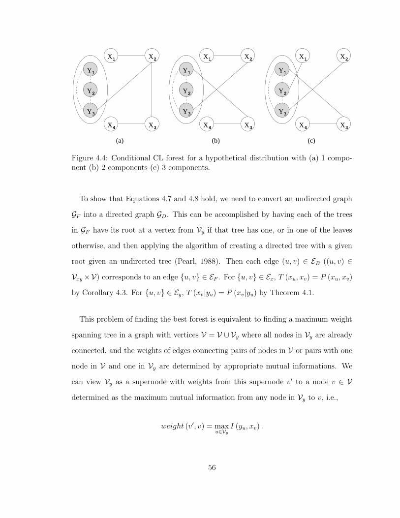
(a) (b) (c)

Y

Y

Y

X

X X

X

Y

Y

Y

X

X X

X

Y

Y

Y

X

X X

X

1

2

3

4

1 2

3

3

2

1

1 2

34 4 3

21

1

2

3

Figure 4.4: Conditional CL forest for a hypothetical distribution with (a) 1 compo-nent (b) 2 components (c) 3 components.

To show that Equations 4.7 and 4.8 hold, we need to convert an undirected graph

GF into a directed graph GD. This can be accomplished by having each of the trees

in GF have its root at a vertex from Vy if that tree has one, or in one of the leaves

otherwise, and then applying the algorithm of creating a directed tree with a given

root given an undirected tree (Pearl, 1988). Then each edge (u, v) ∈ EB ((u, v) ∈

Vxy ×V) corresponds to an edge u, v ∈ EF . For u, v ∈ Ex, T (xu, xv) = P (xu, xv)

by Corollary 4.3. For u, v ∈ Ey, T (xv|yu) = P (xv|yu) by Theorem 4.1.

This problem of finding the best forest is equivalent to finding a maximum weight

spanning tree in a graph with vertices V = V ∪ Vy where all nodes in Vy are already

connected, and the weights of edges connecting pairs of nodes in V or pairs with one

node in V and one in Vy are determined by appropriate mutual informations. We

can view Vy as a supernode with weights from this supernode v′ to a node v ∈ V

determined as the maximum mutual information from any node in Vy to v, i.e.,

weight (v′, v) = maxu∈Vy

I (yu, xv) .

56

Due to the restrictions on the edges, the CCL networks can contain disconnected

tree components (referred to as forests). These CCL forests can consist of 1 to

min |Vy| , |Vx| components. (See Figure 4.4 for an illustration.)

4.3 Beyond Trees

Trees provide flexible and parsimonious distributions for multivariate data; how-

ever, while they are richer than the conditional independence model, the trees are

quite restrictive in structure. This is especially evident in conditional Chow-Liu

forests where due to the restriction of having no more than one parent in a Bayesian

network representation, the conditional distribution splits into multiple subgraphs

and corresponding factors. In this section, we consider models with richer depen-

dency structures, not having the limitations of the tree-structured networks. Poten-

tially, they can be used to model any categorical-valued distribution; however, these

structures lose some of the desirable properties of trees. By leaving the restricted

domain of trees, the search for the optimal structure and the parameters given the

structure are decoupled and cannot be easily performed simultaneously. We also lose

the structure optimality guarantee (Chickering, 1996; Srebro, 2003). As a result,

the algorithms for non-tree structures may have significantly higher computational

complexity than algorithms for tree-structured distributions.

We will utilize Maximum Entropy models, MaxEnt for short, as building blocks

for models when the tree structure for an approximating distribution is undesirable

or insufficient. The MaxEnt model can be viewed as the “smoothest” probability

distribution satisfying constraints on some of its low-dimensional marginals. Consider

an example using the precipitation occurrence modeling as an application.

57

Example 4.1. Assume we have an empirical joint distribution P (x) of occurrence

for five stations with variable Xi corresponding to station i = 1, . . . , 5.6 We want

to approximate our target P with a distribution P (x) which matches all univariate

marginals and also matches the simultaneous rainfall occurrence for a pair of stations

1 and 2, and for a triple of stations 3, 4, and 5:

P (Xi = 1) = P (Xi = 1) , i = 1, . . . , 5,

P (X1 = 1, X2 = 1) = P (X1 = 1, X2 = 1) ,

P (X3 = 1, X4 = 1, X5 = 1) = P (X3 = 1, X4 = 1, X5 = 1) .

Alternatively, the constraints of the marginals can be expressed as

∑

X

P (x) fi (xi) =∑

X

P (x) fi (xi) , i = 1, . . . , 5,

∑

X

P (x) f12 (x1, x2) =∑

X

P (x) f12 (x1, x2) ,

∑

X

P (x) f345 (x3, x4, x5) =∑

X

P (x) f345 (x3, x4, x5)

where functions f called features are defined as

fi (xi) = xi, f12 (x1, x2) = x1x2, and f345 (x3, x4, x5) = x3x4x5.

More generally, we can define features as functions defined on subspaces of X ×Y.

Each feature f is defined as a function f : XDx(f) × YDy(f) → R where Dx (f) ⊆ V

and Dy (f) ⊆ Vy are sets of components of vectors X and Y , respectively, which are

used in defining the feature f . Each feature can be trivially extended to the domain

X × Y by setting f (x,y) = f(

xDx(f),yDy(f)

)

. Let F be the set of features. The

6We are deliberately ignoring the temporal dependence of precipitation in this example.

58

constraint for each feature f ∈ F can be written as

∑

X

∑

Y

P (y) P (x|y) f (x,y) =∑

X

∑

Y

P (x,y) f (x,y) . (4.11)

We will denote a constraint corresponding to a feature f by cf , and the set of such

constraints by C.

Assume that C is consistent. We wish to find a distribution P satisfying all con-

straints in C and also such that P is most similar to some other exponential distribu-

tion Q (x|y), i.e., minimizing KL(

P ‖ Q)

. If Q is uniform on X , this is equivalent to

satisfying C while maximizing the entropy of P , lending the name of the model. Un-

less otherwise specified, we assume thatQ is uniform. By differentiating KL(

P ‖ Q)

with Lagrangians added for constraints in C, we obtain the following functional form

of the solution PME (e.g., see Berger et al., 1996):

PME (x|y) =Q (x|y)

Z (y)exp

(

∑

f∈F

λff (x,y)

)

(4.12)

where Z (y) =∑

X

Q (x|y) exp

(

∑

f∈F

λff (x,y)

)

is a normalization function to enforce∑

X PME (x|y) = 1 with λf ∈ R for all

f ∈ F . Let λ ∈ R|F| be a vector of coefficients λf for this exponential model with

the components of λ indexed by f ∈ F . To specify a MaxEnt model, one needs to

specify the set of features F and then to estimate the set of parameters λ minimizing

KL (P ‖ PME (·|λ,F)).

It is worth pointing out some of the properties of the MaxEnt family of distri-

butions. The set of parameters λ satisfying all of the consistent constraints C also

59

minimizes the relative entropy KL (P ‖ PME), a proxy for a negated log-likelihood

−∑X ,Y P (x,y) lnPME (x|y). This property makes MaxEnt models fit easily in

the maximum likelihood framework of parameter estimation. While the minimum

often cannot be found in closed form, KL (P ‖ PME) is concave as a function of λ,

so the minimum is unique7 (Della Pietra et al., 1997) and can be found by changing

λ in an iterative manner decreasing KL (P ‖ PE) at each iteration.

The dependency network for a distribution from the MaxEnt family can be found

from the domain of its features. The edges E of a Markov network of a distribution

PME (x) or a Conditional Random Field or CRF (Lafferty et al., 2001) for a condi-

tional distribution PME (x|y) consist of pairs of vertices corresponding to variables

of X appearing in at least one feature, i.e.,

E = u, v ∈ V × V : u 6= v and ∃f ∈ F (u ∈ Dx (f) and v ∈ Dx (f)) .

Then features f ∈ F can be seen as specifying potentials on the cliques Dx (f)

with the rest of the cliques (unspecified by features) in the Hammersley-Clifford

decomposition having the potential of 1.

Let us again consider the Example 4.1. The set of features

F = f1, f2, f3, f4, f5, f12, f345 gives rise to the MaxEnt solution

PME (x) =1

Zexp

(

λ1f1 (x1) + λ2f2 (x2) + λ3f3 (x3) + λ4f4 (x4) + (4.13)

+ λ5f5 (x5) + λ12f12 (x1, x2) + λ345f345 (x3, x4, x5))

.

7The distribution satisfying the set of constraints is unique. Depending on the set of constraints,there could be multiple sets of parameters corresponding to the same MaxEnt distribution.

60

v

v

v1

v

v

2

34

5

Figure 4.5: Markov Network for the MaxEnt model in (4.13).

Let V = v1, . . . , v5 with vertex vi corresponding to variable X i, i = 1, . . . , 5.

There are only two constraints, f12 and f345 with domains consisting of more than

two variables. The corresponding Markov network is shown in Figure 4.5.

Tree-structured distributions described in Section 4.2 can also be represented in

the MaxEnt form. Suppose that each variable (either Yu or Xv) can take on one of

B possible values, 0, . . . , B − 1. Let E be the set of edges defined on Vxy × V. The

set of features F would consist of univariate features

fvb (xv) =

1 Xv = b,

0 Xv 6= b,

for v ∈ V and b = 1, . . . , B − 1, and of bivariate features

fuvb1b2 (yu, xv) =

1 Yu = b1 and Xv = b2,

0 otherwise,

∀ (u, v) ∈ E ∩ Vy × V

61

and

fuvb1b2 (xu, xv) =

1 Xu = b1 and Xv = b2,

0 otherwise,

∀ (u, v) ∈ E ∩ V × V

for b1, b2 = 1, . . . , B − 1.

Example 4.2. As another illustration of the models representable in the MaxEnt

form, we consider a model for a joint probability distribution matching all of the

bivariate marginals of the target distribution P (x). We will refer to this model as

a full bivariate MaxEnt model. For simplicity, we assume that X is M -variate with

each variables taking on B values. The set of features F for a MaxEnt model will

consist of B − 1 univariate features

fvb = (xv) =

1 Xv = b,

0 otherwise,

for each of M variables and (B − 1)2 of bivariate features

fuvb1b2 (xu, xv) =

1 Xu = b1 and Xv = b2,

0 otherwise,

for each of M (M − 1) /2 pairs of variables. The Markov network for the model is an

M -vertex clique.

Learning of the MaxEnt model involves the construction of the set of features F

(and the corresponding constraints) and the estimation of the parameters λ. In the

next section (4.3.1), we discuss the estimation of the parameters λ given the set

of features F and the target distribution P (x|y). In Section 4.3.4, we outline an

62

algorithm for the construction of a set of bivariate features and the estimation of its

parameters for a specialized class of distributions built on a MaxEnt model.

4.3.1 Learning Parameters of Maximum Entropy Models

There are a number of algorithms for learning λ by maximizing KL (P ‖ PE) for

a specified set of features F , given the data making up the empirical distribution

P . Early methods optimized the joint probability model (Y = ∅), e.g., iterative

scaling (Brown, 1959; Csiszar, 1975), generalized iterative scaling (GIS) (Darroch

and Ratcliff, 1972); later methods allow the optimization of conditional distributions,

e.g., IS (Jelinek, 1998, page 235), GIS (Rosenfeld, 1994), improved iterative scaling

(IIS) (Berger et al., 1996; Della Pietra et al., 1997), sequential conditional generalized

IS (Goodman, 2002), and a number of methods based on general optimization, e.g.,

gradient descent, conjugate gradient methods (Polak-Ribiere or Fletcher-Reeves), or

second-order methods (e.g., Malouf, 2002). All of the algorithms are computationally

intensive as they require multiple iterations; each iteration requires summation over

all values of Y (which is usually replaced by summing over the Y in the data) and

a summation over all values of X , a number exponential in M . A summation of X

can often be decomposed into lower-dimensional sums (equivalently representable by

message passing methods described later) or replaced by sampling.

We can utilize the structure of the Markov network (or Markov random field) G of

PE to solve the optimization problem by a message passing algorithm that updates

parameters corresponding to the features defined on the cliques of the junction tree

(Jirousek and Preucil, 1995; Bach and Jordan, 2002) and propagates messages with

updates of the probability distributions defined on these cliques to other cliques in

the junction tree. Let J = (CJ , EJ) be a junction tree for G. Recall that the junction

63

Algorithm EfficientMaxEntLearning(P,F ,J )Inputs: Distribution P (X|Y ); a set of features F ; junction tree J capturingconditional independence relationships as assumed by F

1. Initialization:

(a) Assign each λf ∈ λ to one of the cliques C ∈ C such that Dx (f) ⊆ C;

• Denote the set of λf assigned to clique C by λC

• Denote the set of f with λf assigned to C by FC

(b) Set λf = 0 for all f ∈ F

2. Repeat step (3) until convergence

3. Loop through C ∈ C

(a) Set C as the root of J(b) Propagate evidence R from the leaves of J(c) Update λC by decreasing KL (P (xC |y) ‖ PME (xC |y)) (PME from

Equation 4.14) using any of the update algorithms (IIS, GIS, conjugategradients)

Output: Set of coefficients λ minimizing KL (P ‖ PME)

Figure 4.6: Efficient updating of MaxEnt parameters (similar to Bach and Jordan,2002).

tree exists if and only if the corresponding graph G is chordal; if G is not chordal, it

has to be triangulated (made chordal) first. For reasons which will be clear a little

later, we would like to use a triangulation resulting in a decomposable graph with

the smallest total of values of X assignable to each maximal clique. However, the

problem of finding such a triangulation is NP-complete (Arngborg et al., 1987), and

unless the graph is already decomposable (can be efficiently checked by Maximum

Cardinality Search, Tarjan and Yannakakis, 1984), other efficient but possibly subop-

timal algorithms for triangulation are often used instead (e.g., Kjærulff, 1990). After

the maximal cliques are identified, an optimal junction tree can be constructed in a

64

greedy fashion (Jensen and Jensen, 1994). Once the junction tree J for a graph G is

obtained, an update of λ can be performed without summing over all of X but only

over |C| components of X for all maximal cliques C ∈ CJ of G. Bach and Jordan

(2002) described the algorithm for decomposed improved iterative scaling (IIS), but

any algorithm for learning conditional exponential models can be used inside the

loop. A version of this algorithm is shown in Figure 4.6. At the heart of the algo-

rithm is the observation that each update of parameters λ can be decomposed into

updates of subsets of parameters λC corresponding to cliques C ∈ C of the junction

tree. Then each subset of parameters can be updated by first computing evidence

R (xC ,y) =∑

XC

exp(

∑

f 6∈FCλff (x,y)

)

and then updating λC to improve

PME (xC |y) =1

Z (y)R (xC ,y) exp

(

∑

f∈FC

λff (xC ,y)

)

. (4.14)

R (xC ,y) can be computed in a message passing manner by propagating evidence

R from the leaves of the junction tree to the clique C.8 Each evidence propagation

requires summations over all cliques of C; the algorithm can be sped up by not

recomputing the sums for the unchanged paths of J . Updates for each clique requires

summation over all values of X for that clique; this sum has a number of terms

exponential in the size of the clique, so the computational complexity of the algorithm

is at least exponential in the size of the largest clique.

It is worth noting that EfficientMaxEntLearning can also be viewed as a

variation of the Expectation Propagation (EP) algorithm (cf. Minka, 2001).

Example 4.3. To illustrate how the parameter estimation algorithm works, consider

the following setup. Let Y = ∅, X = 0, 16 with corresponding V = a, b, c, d, e, f.8Equation 4.14 can be represented in the form of (4.12) by normalizing R (xC , y).

65

f e

d

cb

a abc

bdf bcf cef

bcbf cf

Figure 4.7: Markov network for the Example 4.3 (left) and its junction tree (right).

Let F = fa, fb, fc, fd, fe, ff , fab, fac, fbc, fbd, fbf , fce, fcf , fdf , fef, and let

PME (x|λ,F) =exp

(

∑

f∈F

)

∑

X exp(

∑

f∈F

)

be a MaxEnt distribution with features defined as fv (x) = xv and fuv (x) = xuxv,

and corresponding parameters

λ = (λa, λb, λc, λd, λe, λf , λab, λac, λbc, λbd, λbf , λce, λcf , λdf , λef). The Markov network

for this distribution is shown in Figure 4.7 (left). This graph is decomposable, and

its junction tree is shown in Figure 4.7 (right).

As the initial step the features and their corresponding parameters are partitioned

into the cliques. For this illustration, we choose the partition

Fabc = fa, fb, fc, fab, fac, fbc, Fbcf = ff , fbf , fcf, Fbdf = fd, fbd, fdf, and Fcef =

fe, fce, fef. For updates, we will set the clique order as (abc, bcf, bdf, cef). To

update λabc = (λa, λb, λc, λab, λac, λbc), we first propagate the unnormalized distribu-

66

tions on the separators of the cliques:

Rbdf (xb, xf ) =∑

Xd

exp

∑

f∈Fbdf

λff (x)

=∑

Xd

exp (λdfd (xd) + λbdfbd (xb, xd) + λdffdf (xd, xf)) ,

Rcef (xc, xf ) =∑

Xe

exp

∑

f∈Fcef

λff (x)

,

Rbcf (xb, xc) =∑

Xf

Rbdf (xb, xf)Rcef (xc, xf ) exp

∑

f∈Fbcf

λff (x)

.

Then λabc is updated to minimize KL(

P (Xabc) ‖ PME (Xabc))

where

PME (Xabc) =Rbcf (xb, xc) exp

(

∑

f∈Fabcλff (x)

)

∑

Xa,Xb,XcRbcf (xb, xc) exp

(

∑

f∈Fabcλff (x)

) .

Next clique to be updated is bcf . First, the evidence is propagated to bcf from the

leaves:

Rabc (xb, xc) =∑

Xa

exp

(

∑

f∈Fabc

λff (x)

)

,

Rbdf (xb, xf) =∑

Xd

exp

∑

f∈Fbdf

λff (x)

(no need to recompute),

Rcef (xc, xf) =∑

Xe

exp

∑

f∈Fcef

λff (x)

(no need to recompute).

67

Then λbcf is updated to minimize KL(

P (X bcf) ‖ PME (Xbcf))

where

PME (Xbcf) =

Rabc (xb, xc)Rbdf (xb, xf)Rcef (xc, xf) exp

(

∑

f∈Fbcf

λff (x)

)

∑

Xb,Xc,Xf

Rabc (xb, xc)Rbdf (xb, xf )Rcef (xc, xf ) exp

(

∑

f∈Fbcf

λff (x)

) .

These updates are applied in sequence to cliques abc, bcf , bdf , and cef until conver-

gence.

4.3.2 Product of Univariate Conditional MaxEnt Model

Let us go back to the original problem of this section. We want to learn a distribu-

tion P (x|y) approximating a distribution P (x|y) without restricting the dependence

structure of P to a tree. In previous subsections, we considered models with undi-

rected representation of the dependence networks. In this subsection, we consider

the directed graph representation for the dependence structure.

Suppose we wish to build an approximation distribution P (x|y) to a target distri-

bution P (x|y) with a given conditional independence structure in the directed graph-

ical form (Bayesian network). As Theorem 4.1 suggests, we can maximize the log-

likelihood or minimize the relative entropy KL(

P ‖ P)

by setting

P(

xv|xpax(v),ypay(v)

)

= P(

xv|xpax(v),ypay(v)

)

thus matching all factors of P to cor-

responding factors of P . Direct application of this approach is often impractical as

the number of parameters needed to specify each factor is exponential in the number

of parent variables thus requiring exponential time complexity in the number of par-

ents for parameter estimation. Also, in practice, P is an empirical distribution com-

puted from data. The number of samples needed to approximate a multi-dimensional

68

grows exponentially with the dimensionality, so a direct assignment of factors of P

is only feasible for small values of |pax (v)| + |pay (v)|. Thus, we may have to resort

to low-dimensional approximation of the factors P(

xv|xpa(v),ypay(v)

)

. Among such

approximations suggested in literature are decision trees (Friedman and Goldszmidt,

1996) and their extension, decision graphs (Chickering et al., 1997). These methods

assume that the entries in the full probability table P(

xv|xpa(v),ypay(v)

)

can be rep-

resented by a small number of values. Thus the conditional probability distribution

for each factor can be represented by these few values and the correspondences of

the values of parent variables to these few values. These models store the above

correspondences in a directed tree or a directed acyclic graph with each leaf node

corresponding to entries in the full probability table of values for parents of the mod-

eled variable in the factor. The graphs are constructed such that the number of

leaves is relatively small compared to the full probability table.

We propose to model each of the factors in the probability distribution by a uni-

variate conditional MaxEnt distribution introduced in the previous subsection. This

representation allows to approximate a full probability table for a conditional dis-

tribution by potentially only a small number of numeric parameters. The MaxEnt

representation does not necessitate the values in the probability table to be mostly

the same; instead, it produces a smooth probability distribution satisfying a num-

ber of constraints imposed by the data. In the remainder of the subsection, we will

describe the model, the estimation of its parameters, and we will point out how the

product of factors of univariate conditional MaxEnt distributions relates to a joint

probability distribution with the collective set of features.

69

We wish to approximate a target distribution P (x|y) by a distribution P (x|y).

Assume that a joint distribution P (x,y) = P (y) P (x|y) has a Bayesian Network

representation GB = Vxy, EB such that there are no edges originating in V and

ending in Vy:

P (x|y) =∏

v∈V

P(

xv|xpax(v),ypay(v)

)

.

Assume that |V| = M . Since GB is a directed acyclic graph, there is an ordering I on

the vertices of V (a bijection of V to 1, . . . ,M) such that the order of all parents

in V of a given node is smaller than the order of that node, i.e., if v = I−1 (i), then

pax (v) ⊆ u = I−1 (k) : k = 1, . . . , i− 1.9 For notational simplicity, let vi denote

the i-th vertex of V under ordering I, i.e., I (vi) = i. We will model each of the

univariate factors P(

xv|xpax(v),ypay(v)

)

as a distribution from the MaxEnt family.

Let Fi be the set of features used to define the above factor. Then ∀f ∈ Fi Dx (f) ⊆

fax (vi) ⊆ v1, . . . , vi and Dy (f) ⊆ pay (vi) ⊆ Vy. Also, vi ∈ Dx (f), or the term

containing f can be cancelled. Each factor can be parametrized as

P(

xvi|xpax(vi),ypay(vi)

)

=exp

(

∑

f∈Fiδff

(

xDx(f),yDy(f)

))

Zi

(

xpax(vi),ypay(vi)

) (4.15)

where Zi

(

xpax(vi),ypay(vi)

)

=∑

Xvi

exp

(

∑

f∈Fi

δff(

xDx(f),yDy(f)

)

)

,

and δf ∈ R. Let δi be the vector of parameters for P(


)

, and let

δ = (δ1, . . . , δM) be the vector of parameters for P (x|y). Let

FPUC = F1 , . . . , FM be the set of feature sets. The functional form of this

9As before, pay (v) ⊆ Vy.

70

Product of Univariate Conditional MaxEnt model (PUC-MaxEnt for short) is then

PPUC−ME (x|y, δ,FPUC) =

M∏

i=1

PME

(

xvi|xpax(vi),ypay(vi), δi,Fi

)

. (4.16)

Given set of features FPUC , the parameter estimation for different factors can be

done independently, i.e., each δi can be estimated independently of other δj, j 6= i.

Any of the iterative algorithms mentioned in Section 4.3.1 can be used to learn the pa-

rameters δi minimizing

KL(

P(


)

‖ PME

(

xvi|xpax(vi),ypay(vi), δi,Fi

))

. However, for this

univariate case, the parameter estimation procedure involves summation only over

the conditioning variables (or data points for empirical distributions) and a single

variable Xvi. A conjugate gradient update algorithm is derived in Appendix A.2.

4.3.3 Connection Between MaxEnt and PUC-MaxEnt Mod-

els

We have described two family of probability distributions, both using MaxEnt

models, to parametrize an approximation to a target conditional distribution

P (x|y). Assume that the total set of features F for both such models is the

same. If we are provided with a Bayesian network and a PUC-MaxEnt distribution

PPUC−ME (x|y, δ,FPUC), we will consider a MaxEnt distribution

PME (x|y,λ,F) with the same set of all features F = ∪Mi=1Fi. If we are pro-

vided with a MaxEnt distribution PME (x|y,λ,F), we can construct a partition

FPUC = F1, . . . ,FM by first choosing an ordering I, and then partitioning F into

M sets by assigning features to the set corresponding to the variable with the highest

order, Fi =

f ∈ F : i = maxu∈Dx(f) I (u)

. The parents of node vi would consist of

71

nodes corresponding to variables appearing in features in Fi:

pax (vi) = u ∈ V \ vi : ∃f ∈ Fv ∧ u ∈ Dx (vi) and

pay (vi) = u ∈ Vy : ∃f ∈ Fv ∧ u ∈ Dy (vi) .

The MaxEnt and PUC-MaxEnt distributions are, respectively,

PME (x|y,λ,F) =exp

(

∑

f∈F λff (x,y))

Z (y)and

PPUC−ME (x|y, δ,FPUC) =exp

(

∑

f∈F δff (x,y))

∏Mi=1 Zi

(

xpax(vi),ypay(vi)

) . (4.17)

In general, a distribution from a PUC-MaxEnt family may not belong to the

MaxEnt family or vice versa as each of the families has certain dependency structure

imposed by the features and the ordering (in the PUC-MaxEnt). This should be

expected as causal models represented by Bayesian (directed) networks and models

represented by Markov (undirected) networks while overlapping do not contain one

another. For the general class of dependence models, the intersection between the

sets of models representable by both Bayesian and Markov networks is the set of

decomposable models with dependencies captured by chordal (decomposable) graphs

(e.g., see Pearl, 1988). For a fixed domain and the total set of features, the space

of models falling into each of PUC-MaxEnt family (directed) and MaxEnt family

(undirected) is even smaller than that of the general models. While their intersection

must also fall within the class of decomposable models, it could possibly be even more

restrictive.

72

In the rest of this subsection, we will briefly investigate the models belonging

to both PUC-MaxEnt and MaxEnt families. We will again consider the setting

of approximating a target distribution P (x|y). Let λ? be the set of parameters

minimizing KL (P ‖ PME (·|λ,F)), and let δ? be the set of parameters minimizing

KL (P ‖ PME (·|δ,FPUC)). By one of the properties of MaxEnt models, parameters

minimizing the relative entropy KL result in a distribution satisfying constraints

associated with each feature. The satisfied constraints are

∑

X

∑

Y

P (y)PME (x|y,λ?,F) f (x,y) =∑

X

∑

Y

P (x,y) f (x,y) (4.18)

for all f ∈ F for MaxEnt model and

∑

Xfax(v)

∑

Y pay(v)

P(

xpax(v),ypay(v)

)

PPUC−ME

(

xv|xpax(v),ypay(v), δ?,FPUC

)

f (x,y)

=∑

X fax(v)

∑

Y pay(v)

P(

xfax(v),ypay(v)

)

f (x,y)

for all v ∈ V for all f ∈ Fi where i = I (v). If a MaxEnt distribution with features

F satisfies constraints in (4.18) for all f ∈ F , then that distribution is the same as

PME (x|y,λ?,F) since such a distribution is unique (e.g., Della Pietra et al., 1997).

By identifying the conditions under which PPUC−ME (x|y, δ?,FPUC) belongs to the

MaxEnt family and satisfies constraints in (4.18) for all f ∈ F = ∪Mi=1Fi, we will

obtain PPUC−ME (x|y, δ?,FPUC) ≡ PME (x|y,λ?,F). The condition of constraint

satisfaction can be addressed under a very strong assumption.

Theorem 4.4. Let I be an ordering of nodes of V as defined on page 70. Assume

73

that satisfying constraints

∑

X

∑

Y

P (y)PPUC−ME (x|y, δ?,FPUC) f (x,y) =∑

X

∑

Y

P (x,y) f (x,y)

for all f ∈ ∪i−1k=1Fk implies P (y)PPUC−ME

(

xpax(v)|y, δ?,FPUC

)

= P(

xpax(v),y)

on

Xpax(vi) × Y, then all of the constraints associated with features in F are satisfied by

PPUC−ME (x|y, δ?,FPUC):

∑

X

∑

Y

P (y)PPUC−ME (x|y, δ?,FPUC) f (x,y) =∑

X

∑

Y

P (x,y) f (x,y) ∀f ∈ F .

The conditions needed for distributions from the PUC-MaxEnt family to belong

also to the MaxEnt family are unclear. For the case of Y = ∅, each of the PUC-

MaxEnt normalization functions Zi

(

xpa(vi)

)

> 0 can be viewed as an unnormalized

probability distributions over Xpa(vi). Let

PZi

(

xpa(vi)

)

= Zi

(

xpa(vi)

)

/

∑

Xpa(vi)

Zi

(

xpa(vi)

)

.

Let Fpa(v) = f ∈ F : D (f) ⊆ pa (v). If for each i = 1, . . . ,M , PZi

(

xpa(vi)

)

can be

represented by a MaxEnt distribution PME

((

xpa(vi)

)

|ξvi,Fpa(vi)

)

, then

PPUC−ME (x|δ?,FPUC) is a member of the MaxEnt family with features F . This

74

result follows from the functional form of the PPUC−ME (Equation 4.17):

PPUC−ME (x|δ,FPUC) =exp

(

∑

f∈F δff (x))

∏Mi=1 Zi

(

xpax(vi)

)

=exp

(

∑

f∈F δff (x))

∏Mi=1 PME

(

xpa(vi)|ξvi,Fpa(vi)

)

M∏

i=1

∑

Xpa(vi)

Zi

(

xpa(vi)

)

−1

=1

Z×

exp(

∑

f∈F δff (x))

∏Mi=1 exp

(

∑

f∈Fpa(vi)

ξvi,ff(

xpa(vi)

)

)

=1

Z× exp

∑

f∈F

δff (x) −M∑

i=1

∑

f∈Fpa(vi)

⊆F

ξvi,ff(

xpa(vi)

)

where

Z =

M∏

i=1

∑

Xpa(vi)

Zi

(

xpa(vi)

)

∑

Xpa(vi)

exp(

∑

f∈Fpa(vi)

ξvi,ff(

xpa(vi)

)

) .

If PPUC−ME (x|δ?,FPUC) satisfies both the condition above and the assumption of

the Theorem 4.4, then

PPUC−ME (x|δ?,FPUC) = PME (x|λ?,F) .

If needed, the correspondence between λ? and δ? can be established as

λ?f = δ?

f −∑

v∈V :D(f)⊆pa(v)

ξv,f ∀f ∈ F .

Example 4.4. Consider the same domain and the same set F of features as in

75

f e

d

cb

a

Figure 4.8: Bayesian network for PUC-MaxEnt distribution in Example 4.4.

Example 4.3. Let

Fa = fa , Fb = fb, fab , Fc = fc, fac, fbc ,

Fd = fd, fbd, fdf , Fe = fe, fce, fef , Ff = ff , fbf , fcf ,

and let FPUC = Fv : v ∈ V. For each variable, we can compute the set of parent

variables by combining the domains of corresponding features and removing the

variable itself: pa (a) = ∅, pa (b) = a, pa (c) = a, b, pa (d) = b, f, pa (e) =

c, f, pa (f) = b, c. A PUC-MaxEnt distribution with a set FPUC of feature sets

is then defined as

PPUC−ME (x|δ,FPUC) =∏

v∈V

PME

(

xv|xpa(v), δv,FPUC

)

with a vector of parameters δ, one parameter per corresponding feature in F . This

PUC-MaxEnt distribution has the conditional independence structure captured by

the Bayesian network shown in Figure 4.8.

76

To check whether PPUC−ME (x|δ,FPUC) can be represented by a MaxEnt distri-

bution, we will examine feature sets Fpa (v) for v ∈ V:

Fpa(a) = ∅, Fpa(b) = fa , Fpa(c) = fa, fb, fab ,

Fpa(d) = fb, ff , fbf , Fpa(e) = fc, ff , fcf , Fpa(f) = fb, fc, fbc .

For this example, each set Fpa(v) can be used with MaxEnt model to model any

probability distribution on Xpa(v). Consider, for example, a bivariate domain Xb,f =

Xpa(d). Any distribution P on Xb,f can be modeled by satisfying constraints

PME (Xb = 1| fb, ff , fbf) =∑

Xb,f

PME (xb, xf | fb, ff , fbf) fb (xb)

=∑

Xb,f

P (xb, xf ) fb (xb) = P (Xb = 1) ,

PME (Xf = 1| fb, ff , fbf) =∑

Xb,f

PME (xb, xf | fb, ff , fbf) ff (xf )

=∑

Xb,f

P (xb, xf ) ff (xf ) = P (Xf = 1) ,

and

PME (Xb = 1, Xf = 1| fb, ff , fbf) =∑

Xb,f

PME (xb, xf | fb, ff , fbf) fbf (xb, xf )

=∑

Xb,f

P (xb, xf ) fbf (xb, xf ) = P (Xb = 1, Xf = 1) .

Thus under this set of features F , the PPUC−ME (x|FPUC) distribution can also be

represented by a MaxEnt distribution PME (x|F). The assumption for Theorem 4.4

holds as well.

77

4.3.4 Selection of Features

Up to this point in this section, we have assumed that the set of features for the

MaxEnt and PUC-MaxEnt models is known. However, for most problems the set of

features is unknown and also has to be learned from the data. Feature selection can

be accomplished by search over the space of allowed feature sets. The objective of the

search is to find the set of features with the highest score, a measure of the goodness

of fit of the resulting distribution to the data. Such a set is usually found by starting

out with an empty set or a random subset of all possible features, and iteratively

changing the set of features until the resulting set is satisfactory. Candidate feature

sets can be obtained from the current ones by simple operations; for example, feature

addition or deletion. The search strategy determines which of the candidates to take

as the new set according to the scores of the candidates.

The algorithm for learning both the structure and the parameters given the struc-

ture can be viewed as two nested loops; the outer loop searches for the structure while

the inner loop optimizes the parameters given the structure (Figure 4.9). There are

a number of possibilities for functions GenerateCandidates, score, and select. The

scoring function should both reflect the goodness of fit of the model with the can-

didate set and to also address potential overfitting. This can be accomplished by

a regularization term. For example, with the Bayesian approach, the regularization

term is a prior on the sets of features possibly penalizing more complex structures

by assigning them a low probability mass. Alternatively, candidate sets can be re-

stricted not to exceed a predefined complexity. Bach and Jordan (2002) consider

sets of features such that the resulting junction tree has bounded width. Finding

the optimal structure is often impractical or intractable (e.g., Chickering, 1996), so a

heuristic approach may be used instead of an exhaustive search. If the set of candi-

78

Algorithm StructureLearning(P,A)Inputs: Distribution P (x,y); a set of all possible features AFunctions:GenerateCandidates () to generate candidate subsets of features;score function Score (); selector Select () to determine which candidate to pickgiven all of the scores; parameter update LearnParameters ()

1. Initialization:

(a) Select initial set of features F ⊆ A(b) Learn parameters λ = LearnParameters (F , P )

2. Loop until convergence

(a) Compute candidate sets CD = GenerateCandidates (λ,F)

(b) For all c ∈ CD• Compute score Score (c,F ,λ, P )

(c) Update set of features F = Select (S) where S = score (c) : c ∈ CD(d) Update the parameters λ = LearnParameters (F , P )

Output: Set of features F and set of coefficients λ

Figure 4.9: Feature selection for exponential models.

dates is constructed in a greedy fashion, new candidates are constructed by adding a

single new feature to the existing set. Alternatively, new candidates can be obtained

by allowing the removal of features from the current set. While we would like the

scoring function to be an accurate predictor for the goodness of fit, we also want

it to be cheap to compute since its computation is inside two nested loops. Some

methods like Minimum Description Length (used by Friedman (1997) for Bayesian

networks structure learning) require parameter learning for each candidate set of

features, a computationally intensive procedure. Methods that only learn the values

of the parameters corresponding to the added features (Della Pietra et al., 1997) are

less accurate but faster computationally. There are many possibilities for selection of

the next set of features; commonly, the next set is selected by choosing a candidate

79

with a highest score (greedy approach).

4.3.5 PUC-MaxEnt Models for Bivariate Interactions of Bi-

nary Data

We illustrate some of the ideas from the previous two subsections by considering a

special case where all of the allowed features are defined on either a single variable or

a pair of binary (0, 1) variables. Multi-site precipitation occurrence modeling (as

described in Section 1.1) serves as one of the motivations as we want our precipitation

occurrence model to capture pairwise interactions between the stations as well as

interactions of observations on consecutive days. We allow three types of features:

• Univariate: v ∈ V fv (xv) = xv;

• Bivariate in X : u, v ∈ V, u 6= v fuv (xu, xv) = xuxv;

• Bivariate in X × Y: u ∈ V, v ∈ Vy fuv (xu, yv) = xuyv.

We will employ PUC-MaxEnt models for this task. One of the reasons for choosing

a model with a causal structure instead of a Markov random field is the need to

model a conditional distribution, so a directed structure is already implied. The set

of features will be constructed in a greedy fashion, adding one feature at a time.

Initially, the set of features will contain only all of the univariate features fv (xv).

Bivariate feature selection problem can then be viewed as edge induction. After the

addition of each edge, only the parameters of the factor affected by the edge need to

be recalculated while the parameters for the other M − 1 factors are left unchanged.

The algorithm is described in Figure 4.10. To score potential directed edges, we use

the Gain function described by Della Pietra et al. (1997). Assume we are considering

80

adding feature f to a set of features Fv for the factor corresponding to node v ∈ V.

Gain is then defined as

Gain (P,FPUC, δ, f)

= maxδf

KL (P ‖ PPUC−ME (·| (FPUC \ Fv) ∪ Fv ∪ f , (δ, δf)))

−KL (P ‖ PPUC−ME (·|FPUC, δ)) ,

the change in divergence between the model with the original set of features, and the

model with the added feature f to Fv where only the corresponding parameter δf is

optimized. Gain is guaranteed to be non-negative as setting δf = 0 makes the diver-

gences equal. Gain is also a lower bound on the change in divergence (log-likelihood)

when all of the parameters are optimized for the new set of features. Gain is reason-

ably fast to compute using an iterative optimization algorithm (Newton-Raphson),

and in practice requires only a small number of iterations. The full parameter up-

date algorithm LearnParameters consists of computing parameters of M univariate

conditional factors. Except for the initialization, only one of the factors requires the

reestimation of its parameters, and this update can be carried out using the equations

in Appendix A.2.

Note that there is no explicit regularization term in the score function. The score

is always non-negative, and by adding extra features to FPUC we are guaranteed not

to decrease the log-likelihood of the data. However, to prevent overfitting, we stop

adding features when the potential improvement in log-likelihood (the Gain score

scaled to the amount of data) becomes too small.

81

Algorithm StructureLearningPUC-MaxEnt(P )Inputs: Distribution P (x,y)Functions: Score function Gain (); parameter update LearnParameters ()

1. Initialization:

(a) Initializing factors: ∀v ∈ Vi. Put univariate features into corresponding factor: Fv = fv (xv)ii. Learn parameters δv = LearnParameters (Fv, P )

(b) Set list of candidate edges to all edges from Vxy to V except for self-loops: C = (u, v) ∈ Vxy × V : u 6= v

(c) Compute scores of the candidates: ∀ (u, v) ∈ Ci. score ((u, v)) = Gain (P,FPUC , δ, fuv)

2. While ∃ (u, v) ∈ C with score ((u, v)) > threshold

(a) Pick best candidate: (u?, v?) = argmax(u,v)∈C score ((u, v))

(b) Update the set of candidates C to remove the loops and repetitionsassociated with adding edge (u?, v?)

(c) Update factor v?:

i. Update the list of features: Fv? = Fv? ∪ fu?v?ii. Update parameters: δv = LearnParameters (Fv, P )

iii. Update scores: ∀ (u, v?) ∈ CA. score ((u, v?)) = Gain (P,FPUC, δ, fuv?)

Output: Set of features FPUC and set of coefficients δ

Figure 4.10: Structure and parameter learning for PUC-MaxEnt.

82

4.4 Other Possibilities

4.4.1 Multivariate Probit Model

Consider a problem related to the setup in Example 4.2. We are given all of the

bivariate marginals of the target distribution P either explicitly or implicitly via a

joint distribution on X = 0, 1M . We want to construct a distribution Q (x) such

that all the bivariate marginals of Q match the corresponding marginals of P , i.e.,

∀ (u, v) ∈ V, P (xu, xv) = Q (xu, xv). Such a distribution Q can then be used to gen-

erate multivariate binary data with specified bivariate distributions. For example, in

precipitation occurrence modeling, this model can be used to simulate multi-site rain-

fall occurrences while preserving pairwise interactions. One possibility is to employ a

maximum entropy model with features ∀u, v ∈ V, f (xu) = xu and f (xu, xv) = xuxv

as described in Example 4.2.10 The drawback of using this maximum entropy

model is that the parameter estimation using iterative proportional fitting or by

another method requires multiple iterations; each iteration requires a re-estimation

of Q (xu, xv) for all u, v ∈ V requiring an exponential number of computations in M

for the exact result. Alternatively, an approximation can be obtained via simulation

or belief propagation, still requiring a large amount of computation. In this section

we consider another type of distribution that can match all bivariate marginal dis-

tributions for the binary-valued multivariate case. This model can be learned very

quickly (in time proportional to M 2), and can be used for generating data that agrees

with P on all pairs of variables.

This model is based on a different parametrization of a binary distribution. We

first consider the univariate case (M = 1). Suppose a random variable X takes

10This model is also sometimes referred to as auto-logistic model.

83

values from −1, 1M .11 There are multiple ways to represent a univariate probability

distribution for the binary domain. The univariate logistic function (a special case

of the exponential model) can be represented as

P (x|λ) =1

1 + exp (xλ)

and can be easily extended to regression. The univariate probit model uses the

cumulative distribution function (CDF) Φ of a univariate normal with zero mean

and unit variance instead:

PPB (x) = Φ (xb) =

∫ b

a

1√2πe−

12t2dt, (4.19)

where

(a, b) =

(−∞, β) for x = 1,

(β,∞) for x = −1.

For the multivariate case, we can model an M -variate binary X using a zero-mean

Gaussian with a unit-diagonal covariance matrix Σ, so for a probit model, the co-

variance matrix of the underlying Gaussian is its correlation matrix. Let ρij be the

correlation between Xi and Xj. Vector β = (β1, . . . , βM) determines the boundaries

of the orthants:

PPB (x) =

∫ b1

a1

. . .

∫ bM

aM

1

(2π)M2 |Σ| 12

e−12t′

Σ−1tdt1 . . . dtM

11It is more convenient for this chapter to use −1, 1 for the binary domain rather than 0, 1used elsewhere in the thesis.

84

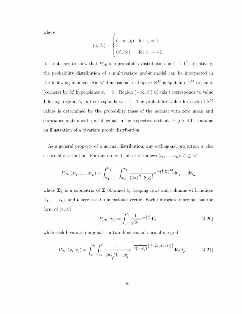
where

(ai, bi) =

(−∞, βi) for xi = 1,

(βi,∞) for xi = −1.

It is not hard to show that PPB is a probability distribution on −1, 1. Intuitively,

the probability distribution of a multivariate probit model can be interpreted in

the following manner. An M -dimensional real space RM is split into 2M orthants

(corners) by M hyperplanes xi = βi. Region (−∞, βi) of axis i corresponds to value

1 for xi; region [βi,∞) corresponds to −1. The probability value for each of 2M

values is determined by the probability mass of the normal with zero mean and

covariance matrix with unit diagonal in the respective orthant. Figure 4.11 contains

an illustration of a bivariate probit distribution.

As a general property of a normal distribution, any orthogonal projection is also

a normal distribution. For any ordered subset of indices (i1, . . . , iL), L ≤ M ,

PPB (xi1 , . . . , xiL) =

∫ bi1

ai1

. . .

∫ biL

aiL

1

(2π)L2 |ΣL|

12

e−12t′

Σ−1L

tdti1 . . .dtiL

where ΣL is a submatrix of Σ obtained by keeping rows and columns with indices

(i1, . . . , iL), and t here is a L-dimensional vector. Each univariate marginal has the

form of (4.19)

PPB (xi) =

∫ bi

ai

1√2πe−

12t2i dti, (4.20)

while each bivariate marginal is a two-dimensional normal integral

PPB (xi, xj) =

∫ bi

ai

∫ bj

aj

1

2π√

1 − ρ2ij

e− 1

2(1−ρ2ij)

(t2i −2ρij titj+t2j)dtidtj. (4.21)

85

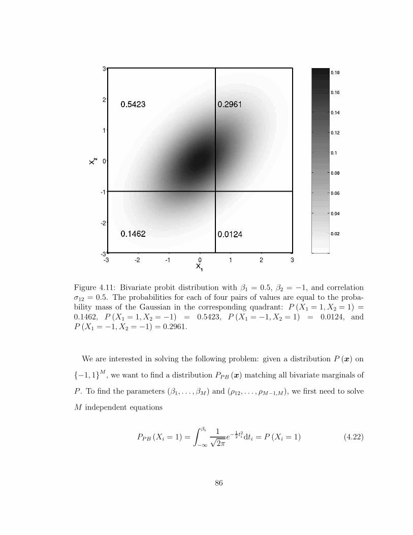
Figure 4.11: Bivariate probit distribution with β1 = 0.5, β2 = −1, and correlationσ12 = 0.5. The probabilities for each of four pairs of values are equal to the proba-bility mass of the Gaussian in the corresponding quadrant: P (X1 = 1, X2 = 1) =0.1462, P (X1 = 1, X2 = −1) = 0.5423, P (X1 = −1, X2 = 1) = 0.0124, andP (X1 = −1, X2 = −1) = 0.2961.

We are interested in solving the following problem: given a distribution P (x) on

−1, 1M , we want to find a distribution PPB (x) matching all bivariate marginals of

P . To find the parameters (β1, . . . , βM) and (ρ12, . . . , ρM−1,M), we first need to solve

M independent equations

PPB (Xi = 1) =

∫ βi

−∞

1√2πe−

12t2i dti = P (Xi = 1) (4.22)

86

to find βi, and then to solve M (M − 1) /2 independent equations

PPB (Xi = 1, Xj = 1) =

∫ βi

−∞

∫ βj

−∞

1

2π√

1 − ρ2ij

e− 1

2(1−ρ2ij)

(t2i −2ρij titj+t2j)dtidtj (4.23)

= P (Xi = 1, Xj = 1) , 1 ≤ i, j ≤M, i 6= j

to find ρij. Equation 4.22 can be solved by taking the inverse of Φ (e.g., Wichura,

1988). Equation 4.23 can be solved as an inverse problem of finding the rectangular

bivariate normal, an integral of a normal distribution over a rectangular region with

boundaries parallel to the coordinate planes; rectangular bivariate normals, in turn,

can be computed with high accuracy (e.g., Genz, 2004).

To sample from PPB (x), we first sample Z ∈ RM from the M -variate normal

N (0,Σ). Then X = (X1, . . . , XM) is determined by

Xi =

1 zi < βi,

−1 zi ≥ βi.

We can employ multivariate probit models to model conditional distributions as

well. For y ∈ RM , we can employ generalized linear models (e.g., McCullagh and

Nelder, 1989) to model PPB (x|y). y can be incorporated into the model by estimat-

ing a matrix Γ such that β = Γy instead of estimating β.

There are a number of problems with using multivariate probit models to ap-

proximate multivariate binary distributions. First, not all multivariate binary dis-

tributions can be represented by a multivariate probit distribution; while all 2 × 2

submatrices of the correlation matrix obtained by selecting i-th and j-th rows and

columns are positive definite, this does not guarantee that the matrix obtained by

87

s

b

d

c

a

b

d

c

a

(a) (b)

Figure 4.12: Example of potential benefits of latent variables. If a latent variable Xs

is included in the model, the Bayesian network (a) of the distribution is sparser andrequires fewer parameters than if Xs is ignored (network (b)).

solving equations 4.22 and 4.23 is positive definite. Second problem, the probit model

does not generalize to domains with more than two values per dimension. Also, the

probability of a vector under the probit model cannot be evaluated exactly except for

a few special cases of the covariance matrix. To evaluate such a probability, we need

to evaluate an M -dimensional rectangular normal integral. While this can be done

accurately for small values of M (e.g., Genz, 1993; Kotz et al., 2000), evaluation of

the integral for larger values of M with good accuracy requires an exponential num-

ber of samples in M . Lastly, while a maximum likelihood estimator for multivariate

probit models exists and is unique (Lesaffre and Kaufmann, 1992), the estimation

cannot be efficiently performed.

4.4.2 Mixtures

As was mentioned in passing, adding hidden variables to the set of observed vari-

ables can sometimes lead to sparser conditional independence structure and, thus, to

fewer free parameters overall. (See Figure 4.12 for an illustration.) In this section,

88

we consider modeling multivariate categorical distributions using nested finite mix-

tures. A finite mixture model for an M -variate categorical random variable X taking

values on X consists of a latent variable Z taking on the values 1, . . . , K, K <∞,

and K mutually independent M -variate categorical probability distributions P iM (x),

i = 1, . . . , K. The probability PM (x) under the mixture model is defined as

PM (x) =

K∑

i=1

P (Z = i)P iM (x) .

The advantage of mixtures is that they allow us to combine probability distribu-

tions with simple dependency structures to create probability distributions capable

of capturing more complex dependency structures. For example, a class of mixtures

of Chow-Liu trees is considerably more expressive than the class models with a sin-

gle tree dependence structure (Meila and Jordan, 2000). Also note that the idea of

mixtures can be extended to allow not one latent variable, but a finite hierarchy of

latent variables; in other words, the categorical probability distributions Pi (x) are

allowed to be mixtures themselves.

Finite mixture models require K parameters π = (π1, . . . , πK to specify

P (Z = i) = πi otherwise called mixing parameters. Since∑K

i=1 πi = 1, only K − 1

of πi are free parameters. Finite mixture models also require parameters ζ =

ζ1, . . . , ζK with ζi specifying P iM (x). Given the parameters, the probability of

a vector X under the mixture model can be expressed as

PM (x|π, ζ) =K∑

i=1

πiPiM (x|ζi) .

Under the framework established earlier in this chapter, we want to learn the

parameters θ = π, ζ to minimize KL (P ‖ PM) where P (x) is the target (and

89

often empirical) probability distribution on X . This can be accomplished by using

the iterative Expectation-Maximization (EM) algorithm (Dempster et al., 1977). In

each iteration of the algorithm, the parameters θ are changed to decrease the objec-

tive function KL (P ‖ PM) (or, alternatively, to increase the log-likelihood l (θ) =

∑

X P (x) lnPM (x|θ)). Given parameters θ and new parameters θ′, the difference

in log-likelihood can be represented as a two component sum (similar to Equations

3.11 and 3.12):

l (θ′) − l (θ) =∑

X

P (x)

K∑

i=1

PM (Z = i|x, θ) lnPM (Z = i,x|θ′)

PM (Z = i,x|θ)

+KL (PM (z|x, θ) ‖ PM (z|x, θ′)) .

Since KL-divergence is always non-negative,

l (θ′) − l (θ) ≥∑

X

P (x)K∑

i=1


PM (Z = i,x|θ),

and l (θ′) − l (θ) can be made non-negative by maximizing

Q (θ′, θ) =∑

X

P (x)

K∑

i=1


= EP

[

EPM(z|x,θ) [lnPM (Z = i,x|θ′)]

]

.

taking into the account constraints imposed on θ′. Each iteration consists of two

steps: E-step, computing PM (Z = i|x, θ) ∝ πiPiM (x|θ) ∀x ∈ X such that P (x) >

0, and M-step, maximizing Q (θ′, θ) with respect to θ′. Under these update rules,

π′i =

∑

X P (x)PM (Z = i|x, θ)∑

X∑K

i=1 P (x)PM (Z = i|x, θ)=∑

X

P (x)PM (Z = i|x, θ) . (4.24)

90

In order to find ζ ′, we need to maximize for each i = 1, . . . , K

∑

X

P (x)PM (Z = i|x, θ) lnP iM (x|ζ ′

i) = C ×∑

X

P i (x) lnP iM (x|ζ′

i) (4.25)

where

C =∑

X

P (x)PM (Z = i|x, θ) and P i (x) =1

CP (x)PM (Z = i|x, θ) . (4.26)

Alternatively, for each i = 1, . . . , K, we can minimize KL (P i ‖ P iM (·|ζ ′

i)) which is

the same form as the original objective function. In practice, P (x) is never explicitly

computed or stored. Instead, each of the of the examples in the original data set is

assigned a weight, and this weight is computed anew for each P i.

4.5 Summary

In this chapter we described models with different degrees of variable dependence

for modeling of multivariate categorical data. Among the contributions of this chap-

ter are several new models for multivariate conditional and joint distributions. Condi-

tional Chow-Liu forests, an extension of Chow-Liu model, is an efficient and provably

optimal in its class model for conditional multivariate distributions. Another new

model, a Bayesian network of conditional maximum entropy models (PUC-MaxEnt)

is an alternative to maximum entropy models for conditional and joint probability

distributions. These and other models presented in this chapter can be used for emis-

sion probability distribution with HMMs as suggested in Section 3.4. Such hidden

Markov models are considered further in Chapter 6.

91

Chapter 5

Models for Multivariate

Real-Valued Distributions

This chapter is a real-valued counterpart to Chapter 4. The emphasis of the

chapter is not to provide a complete overview of methods for modeling multivariate

continuous-valued data, but to show how some of the models in Chapter 4 can be

applied to real-valued data, and to draw contrasts and parallels between categorical

and real-valued cases.

5.1 Independence

Univariate data is usually easier to model than multivariate data. Univariate dis-

tributions have been studied longer; they often have nicer computational properties

than their multivariate extensions, and multivariate counterparts of certain univari-

ate functional forms do not always exist. An easy approach to modeling multivariate

data is to assume independence of individual variables. Assuming a functional form

on each of the marginal probability density functions (PDFs) pI (xi), let θi denote

92

the parameters needed to specify pI (xi), and let us further assume that the θi’s are

mutually independent. Let Θ = (θ1, . . . , θM). Then

pI (x|Θ) =

M∏

i=1

pI (xi|θi) .

If p (x) is a(n) (empirical) PDF defined on RM , then

KL (p (x) ‖ pI (x|Θ)) =

M∑

i=1

KL (p (xi) |pI (xi|θi)) ,

so finding the θi’s minimizing KL (p (x) ‖ pI (x|Θ)) can be done by minimizing

KL (p (xi) ‖ pI (xi|θi)) independently.

5.1.1 Modeling Daily Rainfall Amounts

The functional form of the univariate PDF for each variable depends on the domain

of the data. In the context of precipitation, daily rainfall amounts for a single location

are often modeled using a mixture model consisting of (a) one component, a Dirac’s

delta function δ (x), for zero precipitation, and (b) several other components for non-

zero precipitation. Non-zero daily amounts are often modeled by a K-component

(K ≥ 1) mixture of exponential distributions:

pamounts (x) = π0δ (x) +

K∑

k=1

πkαke−αkx,

where π0, . . . , πK are the mixing probabilities, and αk’s are the parameters of the

exponential distributions. Sometimes, gamma distributions or negative binomial

distributions are used instead of exponentials (Bellone, 2000).

93

5.2 Multivariate Normal Distributions

The multivariate normal distribution is the most studied and most commonly used

probability distribution on multivariate real-valued domains. Among the reasons for

its widespread use are intuition for parameter interpretation, ease of calculation of

marginals, relative ease of parameter estimation.

Suppose that the domain is an M -dimensional space of real numbers R. The

probability density function for a normal distribution is defined in terms of a mean

vector µ ∈ RM and a symmetric positive definite covariance matrix Σ ∈ R

M×M :

pN (x) =1

√

(2π)M |Σ|exp

(

−1

2(x − µ)′ Σ−1 (x − µ)

)

.

It turns out that we can impose conditional independence structure on the variables

of X by constraining the inverse covariance matrix Σ−1 = K = kuvu,v∈V , often

referred to as precision or concentration matrix. Zeros of the concentration matrix

correspond to conditional independence relations of the variables (Lauritzen, 1996,

Proposition 5.2):

kuv = 0 ⇐⇒ pN(

xu, xv|xV\u,v

)

= pN(

xu, |xV\u,v

)

pN(

xv|xV\u,v

)

.

Thus, building a network of conditional independencies for a multivariate Gaussian is

equivalent to selection of zero entries in the concentration matrix, and is often called

covariance selection. Once the selection of zero entries in the concentration matrix

is complete, the non-zero entries in the concentration matrix can either be found in

closed form if the resulting model is decomposable (Lauritzen, 1996, Chapter 5.2),

or by iterative proportional scaling (Speed and Kiiveri, 1986) if the model is not

94

decomposable. For more details, see Lauritzen (1996); Cox and Wermuth (1996);

Whittaker (1990).

In this section, we consider an approximation of a (possibly empirical) PDF p (x)

with a multivariate normal pN (x) subject to minimization of the KL-divergence

KL (p ‖ pN ). We start out with a model with a full covariance matrix (a saturated

model), and then consider a multivariate normal counterpart to Chow-Liu trees, a

tree-structured multivariate normal distribution.

5.2.1 Unconstrained Normal Distribution

If the values of µ and Σ are not constrained (except for the symmetric positive

definite property of Σ), the set of parameters υ = (µ,Σ) consists of M (M + 1) /2

free parameters. Such an unconstrained model has the desirable property of preserv-

ing the correlation between any pair of variables. Also, if bivariate marginals of the

distribution p (x) are bivariate normals, then pN (x) will match them exactly.

To learn the parameters we need to find ν minimizing KL (p ‖ pN (·|ν)), or alter-

natively, maximizing

Q =

∫

M

p (x) ln pN (x|υ) dx

= −1

2

∫

M

p (x)(

M ln (2π) − ln |K| + (x − µ)′ K (x − µ))

dx.

By taking the partial derivative of Q with respect to µ we obtain

∂Q

∂µ=

∫

M

p (x)K (x − µ) dx = K (Ep (X) − µ) . (5.1)

95

By setting the derivative to 0, we obtain a maximum likelihood estimate µ = Ep (X).

Before taking the partial derivative with respect to K, we note that for any A,B ∈

RM×M ,

d |A|dA

= 2A−1 − diag(

A−1)

anddtr (AB)

dA= B + Bt − diag (B) .

Then noticing that (x − µ)′ K (x − µ) = tr(

K (x − µ) (x − µ)′)

, we find

∂Q

∂K=

1

2

∫

M

p (x)

(

∂ ln |K|∂K

− ∂

∂Ktr(

K (x − µ) (x − µ)′)

)

dx

=1

2

∫

M

p (x) (2Σ − diag (Σ)) dx

−1

2

∫

M

p (x)(

2 (x − µ) (x − µ)t − diag(

(x − µ) (x − µ)t))dx.

By setting ∂Q∂K

to zero, and by using µ = Ep (X), we find that

Σ = Covp (X) =

∫

M

p (x) (x − Ep (X)) (x − Ep (X))′ dx.

Assuming p is an empirical distribution collected from N samples, the parameters

of the saturated model can be obtained in time O (NM +NM 2) = O (NM2) with

storage requirements of O (M 2). Curiously, the corresponding problem for M -variate

binary data, finding parameters of a distribution from an exponential family matching

all bivariate marginals, would be much more intensive computationally. Not only

there is no closed form solution for multivariate categorical data, this problem is

usually solved using iterative scaling (see Section 4.3), and each iteration requires

the computation of P (xv) and P (xu, xv) for some pair u, v ∈ V. Unfortunately,

for exponential models for binary data, there is no efficient way to compute these

marginals. The exact computation requires the summation over all other variables

96

of X, an O(

2M−1)

time complexity.

In order to compute pN (x|ν), one needs to compute K and |Σ| first, with time

complexity O (M 3)1, and each evaluation of pN (x|ν) will require O (M 2) operations.

Moreover, if N ≤ M , the resulting estimate Σ would be singular and thus not

positive definite (Lauritzen, 1996, Theorem 5.1). Also, when Σ is close to singular,

the accuracy of the inverse operation is severely hindered by the round-off error.

To sample from pN (x|ν), we first need to compute a Cholesky decomposition

Σ = LL′ where L is a lower-triangular matrix. Then a random sample X ∼ N (µ,Σ)

can be obtained as X = µ+LY where Y ∼ N (0, IM), and IM is the M×M identity

matrix, an O (M 2) operation for each sample.

By discovering conditional independence relations in the variables of X,, otherwise

known as covariance selection, we are able to reduce not only the number of samples

needed to estimate Σ (Lauritzen, 1996, Proposition 5.9), but also the computational

complexity of evaluation of and sampling from pN (x|µ,Σ).

5.2.2 Tree-Structured Normal Distributions

As in Section 4.2, we will use tree-structured dependency between variables to specify

the normal distribution. As with Chow-Liu trees for categorical data, we want the

approximating probability distribution to be represented as a normalized product of

the bivariate probability distributions on its edges. Let pNCL (x) denote a normal

distribution with such tree structure. Assume the dependency tree structure GT =

1The inverse matrix could be computed with better asymptotic complexity by more involvedalgorithms or by algorithms using parallel computation.

97

(V, ET ) is known. Then,

pNCL (x) =

(

∏

v∈V

pN (xv)

)

∏

(u,v)∈ET

pN (xu, xv)

pN (xu) pN (xv)

.

For v ∈ V, assume pN (xv) has mean µv and variance σ2v . For each edge u, v ∈ ET ,

assume pV (xu, xv) has parameters

µuv = (µu, µv)′ and Σuv =

σ2u σuσvruv

σuσvruv σ2v

where ruv ∈ (−1, 1). Then

pN (xu, xv)

pN (xu) pN (xv)

=1

√

1 − r2uv

exp

−r2uv

(

xu−µu

σu

)2

+ r2uv

(

xv−µv

σv

)2

− 2ruv

(

xu−µu

σu

)(

xv−µv

σv

)

2 (1 − r2uv)

.

pNCL (x) is an M -variate Gaussian,

pNCL (x) =∏

v∈V

pN(

xv|µv, σ2v

)

∏

u,v∈ET

pN (xu, xv|µuv,Σuv)

pN (xu|µu, σ2u) pN (xv|µv, σ2

v)

=

(2π)M∏

v∈V

σ2v

∏

u,v∈ET

(

1 − r2uv

)

− 12

× exp

(

−1

2

∑

u∈V

∑

v∈V

Kuv (xu − µu) (xv − µv)

)

,

98

with mean µCL = µvv∈V and covariance matrix ΣCL such that Σ−1 = KCL =

Kuvu,v∈V can be computed as

Kuv =

1σ2

vv

(

1 +∑

u:u,v∈ET

r2uv

1−r2uv

)

u = v,

− ruv

|σuσv |(1−r2uv)

u, v ∈ ET ,

0 u, v 6∈ ET and u 6= v.

The covariance matrix ΣCL can be efficiently computed in closed form. Let RCL

be the correlation matrix of pN−CL, so ΣCL = VRCLV where V is a diagonal

matrix with entries Vvv = |σvv|, and R−1CL = VKCLV.2 We will utilize the tree

property of GT : for any pair of distinct vertices (u, v) ∈ V×V, there is a unique path

Puv = (u, . . . , v) connecting u and v. Let |Puv| be the number of nodes in the path

Puv, and let Puv (i) be the i-th node on the path Puv. We are now ready to compute

the correlation matrix RCL.

Theorem 5.1. The correlation matrix RCL = ruvu,v∈V of a tree-structured multi-

variate normal distribution pNCL (x) is

ruv =

1 u = v,

∏|Puv |−1i=1 rPuv(i)Puv(i+1) u 6= v.

(5.2)

Proof. Let A = auvu,v∈V be a matrix with auv = ruv defined as in (5.2), and let

B = buvu,v∈V = R−1CLA. Since both R−1

CL and A are symmetric, AR−1CL = R−1

CLA =

B. We will show that B = IM which would mean that A = RCL.

Let R−1CL = r′uvu,v,∈V where R−1

CL = VKCLV. First, we compute the entries on

the diagonal of B. Let di (u) = V \ (u ∪ ne (u)) be the set of vertices not adjacent

2We assume |V| > 0.

99

w

zu v

Figure 5.1: Illustration of the unique path property of the tree. For two nodesu, v ∈ V, there is a unique neighbor z of u on the path from u to v.

to u (i.e., distant). Then

buu =∑

v∈V

r′uvauv = r′uuauu +∑

v∈ne(u)

r′uvavu +∑

v∈di(u)

r′uvavu

=

1 +∑

v∈ne(u)

r2uv

1 − r2uv

+∑

v∈ne(u)

(

− ruv

1 − r2uv

)

ruv +∑

v∈di(u)

0 × avu = 1.

Non-diagonal entries are somewhat trickier to compute:

buv =∑

w∈V

r′uwawv = r′uuauv +∑

w∈ne(u)

r′uwawv +∑

w∈di(u)

r′uwawv

=

1 +∑

w∈ne(u)

r2uw

1 − r2uw

auv +∑

w∈ne(u)

(

− ruw

1 − r2uw

)

awv +∑

w∈di(u)

0 × awv.

By the property of the tree, when u 6= v, there is exactly one path Puv connecting

u and v. Among the neighbors ne (u), there is a unique node belonging to Puv.

(Existence of more than one neighbor of the starting point belonging to the path

would result in a cycle.) We will denote that node by z = Puv (2). (See Figure 5.1.)

100

Then

auv =

|Puv |−1∏

i=1

rPuv(i)Puv(i+1) = rPuv(1)Puv(2)

|Puv |−1∏

i=2

rPuv(i)Puv(i+1)

= ρuzζzv.

For other neighbors of u, a path from them to v consists of the edge to u and the

path from u to v (see Figure 5.1):

∀w ∈ ne (u) \ z , Pwv = (w, u, . . . , v) ,

Pwv (i) =

w i = 1,

Puv (i− 1) i = 2, . . . , |Puv| + 1,

awv = rwuauv.

Going back to buv,

buv =

1 +∑

w∈ne(u)

r2uw

1 − ρ2uw

auv −∑

w∈ne(u)

ruw

1 − r2uw

awv

=

1 +∑

w∈ne(u)

r2uw

1 − r2uw

auv −ruzazv

1 − r2uz

+∑

w∈ne(u)\z

ruwawv

1 − r2uw

=

1 +∑

w∈ne(u)

r2uw

1 − r2uw

auv −auv

1 − r2uz

+∑

w∈ne(u)\z

r2uwauv

1 − r2uw

= auv

1 +∑

w∈ne(u)

r2uw

1 − r2uw

− 1

1 − r2uz

+∑

w∈ne(u)\z

r2uw

1 − r2uw

= auv

(

1 +r2uz

1 − r2uz

− 1

1 − r2uz

)

= 0.

Thus B = IM , and A = RCL.

The result can be extended to forests as well. To see this, we can connect the

101

trees in the forest into one tree with added edges having correlations set to 0.

For each v ∈ V, we can convert GT into a directed tree with root v. Then pNCL (x)

can be rewritten as

pNCL (x) = pN (xv)∏

u,pa(u)∈ET

pN(

xu, xpa(u)

)

pN(

xpa(u)

) = pN (xv)∏

u∈V\v

pN(

xu|xpa(u)

)

,

pN(

xu|xpa(u)

)

=1

√

2πσ2u|pa(u)

exp

(

−1

2

(

xu − µu|pa(u)

σu|pa(u)

)2)

,

σ2u|pa(u) = σ2

u

(

1 − r2u,pa(u)

)

, µu|pa(u) = µu −ruvσu (xv − µv)

σv.

The objective function, the KL-divergence between the target distribution and the

tree-structured normal, can be written as

KL (p ‖ pNCL) =

∫

M

p (x) logp (x)

pN (xv)∏

u∈V\v pN(

xu|xpa(u)

)dx

= KL (p (xv) ‖ pN (xv))

+∑

u∈V\v

KL(

p(

xu|xpa(u)

)

‖ pN(

xu|xpa(u)

))

.

Each of the KL-divergences can be optimized independently from others. The re-

sulting maximum likelihood estimate of the mean parameters is µCL = Ep (X);

estimates of univariate variances are σ2v = V arp (Xv) for v ∈ V, and correlations for

edge variables ruv = ρuv = Ep(Xu−µu)(Xv−µv)√σ2

uσ2v

. The rest of the entries in the correlation

matrix can be found using the expression of the Theorem 5.1.

102

5.2.3 Learning Structure of Tree-Structured Normal Distri-

butions

We are now interested in finding a set of edges ET for the Chow-Liu tree to minimize

KL (p ‖ pNCL) =

∫

M

p (x) ln p (x) dx

−∫

M

p (x) ln

∏

v∈V

pN (xv)∏

(u,v)∈ET

pN (xu, xv)

pN (xu) pN (xv)

dx

= −Hp [X] −∑

v∈V

∫

p (xv) ln pN (xv) dxv

−∑

(u,v)∈ET

∫

∫

p (xu, xv) ln

pN (xu, xv)

pN (xu) pN (xv)dxudxv. (5.3)

Expression (5.3) is independent of ET , so to find the set of edges ET , we need to

minimize (5.3) (or to maximize its negative). Let

MIp (xu, xv) =

∫

∫

p (xu, xv) ln

pN (xu, xv)

pN (xu) pN (xv)dxudxv. (5.4)

Just as with the categorical case, to minimize KL (p ‖ pNCL), we need to find

tree edges ET maximizing∑

u,v∈ETMIp (xu, xv) which is equivalent to solving a

maximum spanning tree problem for a complete graph with nodes V and weights

MIp (xu, xv) for edges u, v. It turns out that the mutual information MIp depends

only on the correlation coefficient ρuv. First, we simplify the expression inside the

log:

pN (xu, xv)

pN (xu) pN (xv)(5.5)

=1

√

1 − r2uv

exp

−r2uv

(

xu−µu

σu

)2

+ r2uv

(

xv−µv

σv

)2

− 2ruv

(

xu−µu

σu

)(

xv−µv

σv

)

2 (1 − r2uv)

.

103

Then from (5.4)-(5.5)

MIp (xu, xv) = −1

2ln(

1 − r2)

+ruv

1 − r2uv

Ep

[(

Xu − µu

σu

)(

Xv − µv

σv

)]

− r2uv

2 (1 − r2uv)

(

Ep

[

(

Xu − µu

σu

)2]

+ Ep

[

(

Xv − µv

σv

)2])

= −1

2ln(

1 − ρ2uv

)

+ρuv

1 − ρ2uv

× ρuv −ρ2

uv

2 (1 − ρ2uv)

(1 + 1)

= −1

2ln(

1 − ρ2uv

)

.

Note that for ρuv ∈ [0, 1), −12ln (1 − ρ2

uv) is a strictly increasing function, so we

can use |ρuv| instead of −12ln (1 − ρ2

uv) for the MST problem. We should also note

that the Chow-Liu algorithm chooses the edges to minimize the determinant of the

covariance matrix:

|ΣCL| = minGT

∏

v∈V

σ2v

∏

u,v∈ET

(

1 − ρ2uv

)

.

In order to find the parameters of a tree structure, we need to compute correla-

tions for all pairs of variables, O (NM 2) computational task. Selecting the maximum

spanning tree can be done in the same manner as for categorical data, by Kruskal’s

algorithm, O (M 2) task (Cormen et al., 1990). Pelleg and Moore (2003) suggest ac-

celerating the algorithm by approximating the correlations for low-correlation pairs

while reducing computation by ignoring some of the data entries. Once the param-

eters are computed, the computation of pNCL (x) can be performed in only O (M)

(as compared to O (M 2) for the saturated model.) A generation of a single sample

from pNCL (x) would also require O (M) as we do not need to compute the Cholesky

decomposition of ΣCL explicitly. Instead, we can convert GT into a directed tree

(O (M)), and then generate a sample for each variable given its predecessor using

104

univariate conditional distributions.

5.3 Summary

In this chapter, we presented real-valued counterparts to several models for multi-

variate categorical data. We described conditionally independent mixtures of delta

and exponential distributions, applicable to modeling of rainfall amounts. For con-

trast with full bivariate exponential distribution, we described commonly known

normal distribution with full covariance and listed some of its properties. Finally,

we reintroduced a multivariate normal distribution with tree-structured covariance

matrix and described its advantages over the full covariance model. We also derived

a closed form expression for the covariance matrix of the tree-structured normal

distribution.

Tree-structured normal distributions were first described by Zarutskij (1979, 1980).

While the model is very efficient, does not require large amount of data to train, and

is easy to implement, it is rarely mentioned in the literature (e.g., Raudys, 2001).

The closed form expression for the tree-structured covariance matrix has not been

noted before although Whittaker (1990) considers the functional form of a correlation

matrix with conditional independence with three variables.

105

Chapter 6

Putting It All Together: HMMs

with Multivariate Emission Models

In Chapter 3, we described how HMMs can be thought of as a combination of

models for the transition layer P (S|X) and the emission layer P (R|S) (e.g., Equation

3.5).

As discussed in Chapter 3, the set of HMM parameters Θ consists of transition

parameters Ω and emission parameters Υ. Further, Υ consists of parameters corre-

sponding to each value of the hidden state variable S with P (r|S = i, rprevious,Υ) =

P (r|S = i, rprevious,φi,υi) where φi are the parameters specifying the conditional

independence structure for hidden state i, and υi are the parameters of the proba-

bility distribution specified by φi. Structures φi are fixed for some of the emission

models (e.g., independence, full bivariate MaxEnt), and are learned for others (e.g.,

Chow-Liu trees, PUC-MaxEnt). Further, if the structure is learned, it can either be

learned independently for different hidden states (i.e., it is allowed φi 6= φj for i 6= j)

106

or constrained to be shared across all hidden states (φi = φj for all i, j).1 For the

rest of the thesis, whenever the conditional independence structure for the states is

learned, we assume that it is learned independently for all hidden states.

Parameter estimation is performed by the Baum-Welch algorithm as described in

Section 3.3. Each iteration of the algorithm updates the parameters Θr to Θr+1

maximizing the data log-likelihood from iteration r to r + 1. Iterations consist

of two steps: the E-step, computing posterior distributions P (Snt|Rn,1:T ,Θr) and

P (Snt, Sn,t−1|Rn,1:T ,Θr); the M-step, estimating new parameters Θr+1. For the E-

step of HMM parameter learning, the computational complexity is

O (NTK (K +Rtime)), and the space complexity is O (NTK2 +Rspace). Compu-

tation of P (Rnt|Rn,t−1,Snt,Θr) has computational complexity O (Rtime) and space

complexity O (Rspace), and is determined by the emission probability type. For the

M-step, the estimation of the transition probabilities can be performed in O (NTK2)

time and space2; the estimation of Υr+1 depends on the emission type.

In this chapter, we put together the hidden state models discussed in Chapter 3

with multivariate models discussed in Chapters 4 and 5, and compare their compu-

tational complexities and properties.

6.1 HMM with Conditional Independence

We will denote by HMM-CI (or NHMM-CI) a model which uses the independence

model described in Section 4.1 for the emission distributions P (r|S).3 The indepen-

1This choice can be thought of as a bias-variance trade-off (Bilmes, 2004).2For NHMMs, estimation of the transition parameters depends on the dimensionality of the

input variables and the optimization algorithm.3Independence becomes conditional on the value of the hidden state S.

107

dence structures φi are known (see Figure 6.1 (a) for the Bayesian network structure);

a set υi of emission parameters for state i consist of

υi = pimb = P (Rtm = b|St = i) : m = 1, . . . ,M, b = 0, . . . , B − 1 .

The total number of free emission parameters for an HMM-CI is KM (B − 1). As

was shown in Section 3.4, in order to update the values of the emission parameters

in the E-step of the EM-algorithm, we need to minimize the KL-divergence between

Pi (r) as defined in Equation 3.19 and P(

r|S = i,υr+1i

)

. Combining with (4.1), we

get the following update rules for Υr+1:

pimb = Pi (rm = b) =

∑

rntm=bWnt (i)∑N

n=1

∑Tt=1Wnt (i)

=

∑

rntm=bAnt (i)∑N

n=1

∑Tt=1Ant (i)

where Ant (i) = P (Snt = i|rn,1:T ,xn,1:T ,Θr).

This basic model has two advantages over more complicated models: it has few

parameters, and the M-step update of the emission parameters can be performed

quickly, in O (NTKMB). In addition, it often has a straightforward interpretation

in the application domain. While this model does not explicitly model multivariate

interactions between variables of r and between the variables at different time steps,

it does so indirectly via hidden states. As the results in Chapter 8 show, this simple

model can sometimes be as effective as more complex models while requiring only

a fraction of parameters and training time. On the other hand, models that model

variables interactions directly can often achieve better prediction accuracy and often

obtain so with fewer hidden states (smaller K value) .

108

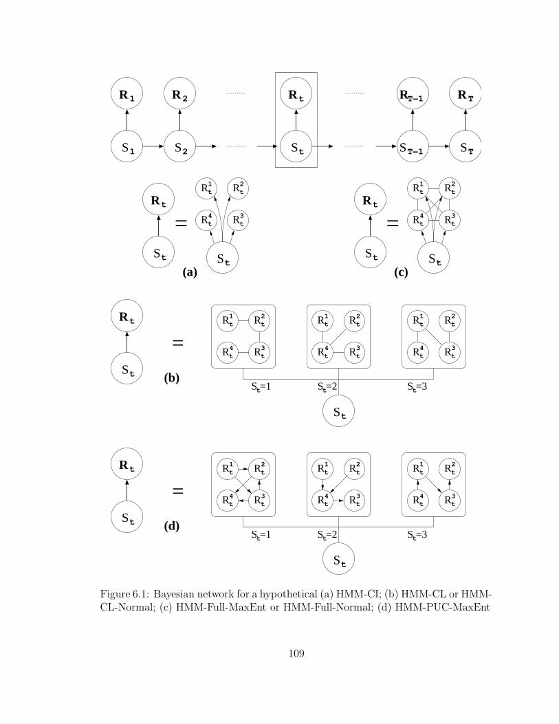
TRRT−1

STST−1

tR

St

2R

S2

tR

St

tR

St

tR

St

1R

S1

St

St

tR

St St St(c)

= R

R1 R2

R3

t

t4t

t

=

S =2 S =3t t t

R1 R2t

3t

1t R2

t

R3t

4t R4

t

R1t R2

t

R3t

S =1(b)

t

Rt4 R

R

R

=

S =2 S =3t t t

R1 R2t

3t

1t R2

t

R3t

4t R4

t

R1t R2

t

R3t

S =1

t

Rt4 R

R

R

(d)

(a)

= R

R1 R2

R3

t

t4t

t

Figure 6.1: Bayesian network for a hypothetical (a) HMM-CI; (b) HMM-CL or HMM-CL-Normal; (c) HMM-Full-MaxEnt or HMM-Full-Normal; (d) HMM-PUC-MaxEnt

109

6.1.1 AR-HMM with Conditional Independence

By combining an autoregressive HMM with the model described in Equation 4.2

(and Figure 4.1, right) we obtain a model for which the Bayesian network is described

by Figure 6.2 (a). We will denote this model by HMM-Chains. Just as with the

HMM-CI, the conditional independence structures φi are known. The set of emission

parameters

υi = pimbb′ = P (Rtm = b|St = i, Rt−1,m = b′) : m = 1, . . . ,M, b, b′ = 0, . . . , B − 1

∪ pimb = P (R1m = b|S1 = i) : m = 1, . . . ,M, b = 0, . . . , B − 1

has M (B2 − 1) free parameters for a total KM (B2 − 1) of free emission parameters.

The E-step update of the parameters is as straightforward as for HMM-CI:

pimbb′ = Pi (rm = b|rprev,m) =

∑

rntm=b

rn,t−1,m=b′Wnt (i)

∑

rn,t−1,m=b′ Wnt (i)=

∑

rntm=b

rn,t−1,m=b′Ant (i)

∑

rn,t−1,m=b′ Ant (i)

and pimb =

∑

rn1m=bAn1 (i)∑N

n=1An1 (i).

If there are only a small number of series available, the probabilities of the first entry

can be estimated from the whole data set:

pimb =

∑

rntm=bAnt (i)

∑Nn=1

∑Tt=1 Ant (i)

.

The E-step update of the emission parameters can be performed in O (NTKMB2)

time, almost the same as for HMM-CI for small B.

110

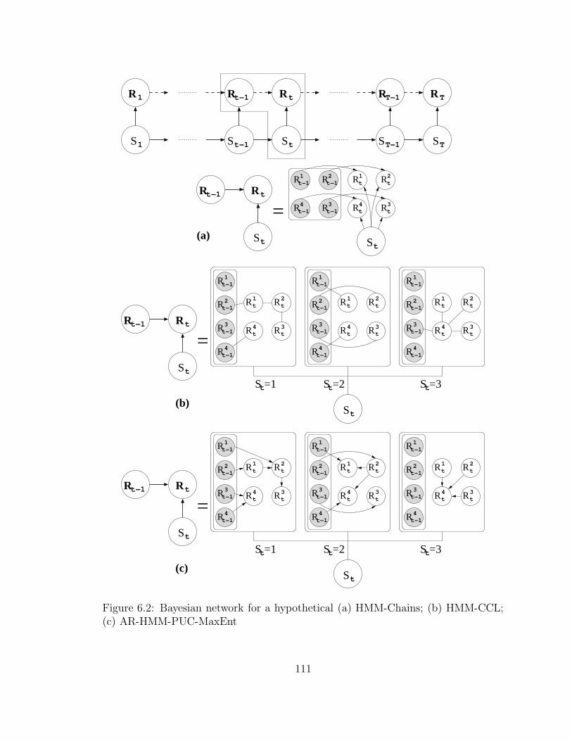
1R

S1

TRRT−1

STST−1

Rt−1

S

tR

Stt−1

R Rt−1 t

St

R R

St

t−1 t

R Rt−1 t

S

St

St

St

t

1

2

3

4

R

R

R

R

t−1

t−1

t−1

t−1

t4R t

3R

t2Rt

1R

1

2

3

4

R

R

R

R

t−1

t−1

t−1

t−1

t4R t

3R

t2Rt

1R

1

2

3

4

R

R

R

R

t−1

t−1

t−1

t−1

t4R t

3R

t2Rt

1R

=

(c)

1

2

3

4

R

R

R

R

t−1

t−1

t−1

t−1

t4R t

3R

t2Rt

1R

Rt

Rt4 R3

Rt2

tRt−13

1t−1

1

Rt−1

t−1R2R

4

(a)

=

1

2

3

4

R

R

R

R

t−1

t−1

t−1

t−1

t4R t

3R

t2Rt

1R

1

2

3

4

R

R

R

R

t−1

t−1

t−1

t−1

t4R t

3R

t2Rt

1R

=

(b)

S =1 S =2t S =3tt

S =1t S =2t S =3t

Figure 6.2: Bayesian network for a hypothetical (a) HMM-Chains; (b) HMM-CCL;(c) AR-HMM-PUC-MaxEnt

111

6.1.2 Application to Multi-Site Precipitation Modeling

As mentioned in Section 5.1.1, rainfall amounts for individual stations are some-

times modeled as a mixture of exponentials. A useful model is a mixture of a Dirac

delta functions and C exponentials (conditionally independent given the state)

p (rnt|Snt = i) =

M∏

m=1

p (rntm|Snt = i) where

p (rntm|Snt = i) =

πim0 rntm = 0

∑Cc=1 πimcαimc exp (−αimcrntm) rntm > 0

with πimc ≥ 0 and∑C

c=0 πimc = 1. This model (from Section 5.1.1) can be used as

the emission model with HMMs, and in this manner we create a model capable of

producing realistic daily precipitation amount simulations. The Bayesian network

for this model is the same as for HMM-CI (Figure 6.1 (a)). Bellone (2000) suggests

using a two-component mixture with a gamma or a negative binomial distribution

instead of the exponential distributions.

The E-step update of π’s and α’s can be performed using the methodology de-

scribed in Section 4.4.2. To compute the updated probabilities in Expressions 4.24

and 4.25, we first need to compute the posterior probabilities of the mixture compo-

112

nents picntm = P (Cntm = c|Snt = i, rntm):

picntm =

πimcp (rntm|Snt = i)∑C

c=0 πimcp (rntm|Snt = i)

=

1 c = 0, rntm = 0,

0 c 6= 0, rntm = 0 or c = 0, rntm > 0,

πimcαimc exp(−αimcrntm) C

c=1 πimcαimc exp(−αimcrntm)c 6= 0, rntm > 0,

and then to update the probability distributions in Equation 4.26. Equivalently, we

update the weights Wnt (i) from Equation 3.18, setting the new weights to Wnt (i)×

picntm. Then the π parameters can be updated as

πimc =

∑Nn=1

∑Tt=1Wnt (i) p

icntm

∑Nn=1

∑Tt=1

∑Cc=0Wnt (i) pic

ntm

=

∑Nn=1

∑Tt=1 Ant (i) p

icntm (i)

∑Nn=1

∑Tt=1Ant (i)

with the mixing probability for zero rainfall identical to the update rule for no pre-

cipitation for the categorical case:

πim0 =

∑

n,t

rnt=0Ant (i)

∑Nn=1

∑Tt=1Ant (i)

.

To update λ’s, we first need to recall that to minimize KL (p (x) ‖ α exp (−αx)),

α = [Ep (X)]−1. Then

αimc =

[

∑Nn=1

∑Tt=1 Wnt (i) p

icntmrntm

∑Nn=1

∑Tt=1Wnt (i) p

icntm

]−1

=

∑Nn=1

∑Tt=1 Ant (i) p

icntm

∑Nn=1

∑Tt=1Ant (i) pic

ntmrntm

.

The computation required for the update is then O (NTMC) to compute picntm,

O (NTMC) to update π’s and α’s. If the data has relatively few precipitation oc-

currences, the computation can be sped up to O (# (rntm = 0) + C × # (rntm = 1)).

113

6.2 HMM with Chow-Liu Trees

The HMM-CI and HMM-Chain models can often be too simplistic in real applica-

tions since they do not capture direct interactions between the components of Rnt.

Chow-Liu trees are designed to capture some such multivariate dependencies. In this

section, we described a model obtained by using Chow-Liu tree distributions as the

emission probability distributions for HMMs. We can use HMMs with Chow-Liu

trees or conditional Chow-Liu forests to model the output variable given the hidden

state. HMMs can model the temporal structure of the data while the Chow-Liu mod-

els can capture “instantaneous” dependencies between multivariate outputs as well as

additional dependence between vector components at consecutive observations over

time that the state variable does not capture.

By combining HMMs with the Chow-Liu tree model and with the conditional

Chow-Liu forest model we obtain HMM-CL and HMM-CCL models, respectively.

The set of parameters Θ for these models with K hidden states and B-valued M -

variate vector sets consists of a K×K transition matrix Γ, a K×1 vector Π of prob-

abilities for the first hidden state in a sequence, and Chow-Liu trees or conditional

forests Ti (r|rprevious) with parameters (φi,υi) for each hidden state i. Examples

of graphical model structures for both the HMM-CL and HMM-CCL are shown in

Figure 6.1 (b) and 6.2 (b), respectively. The likelihood of Θ can then be computed

114

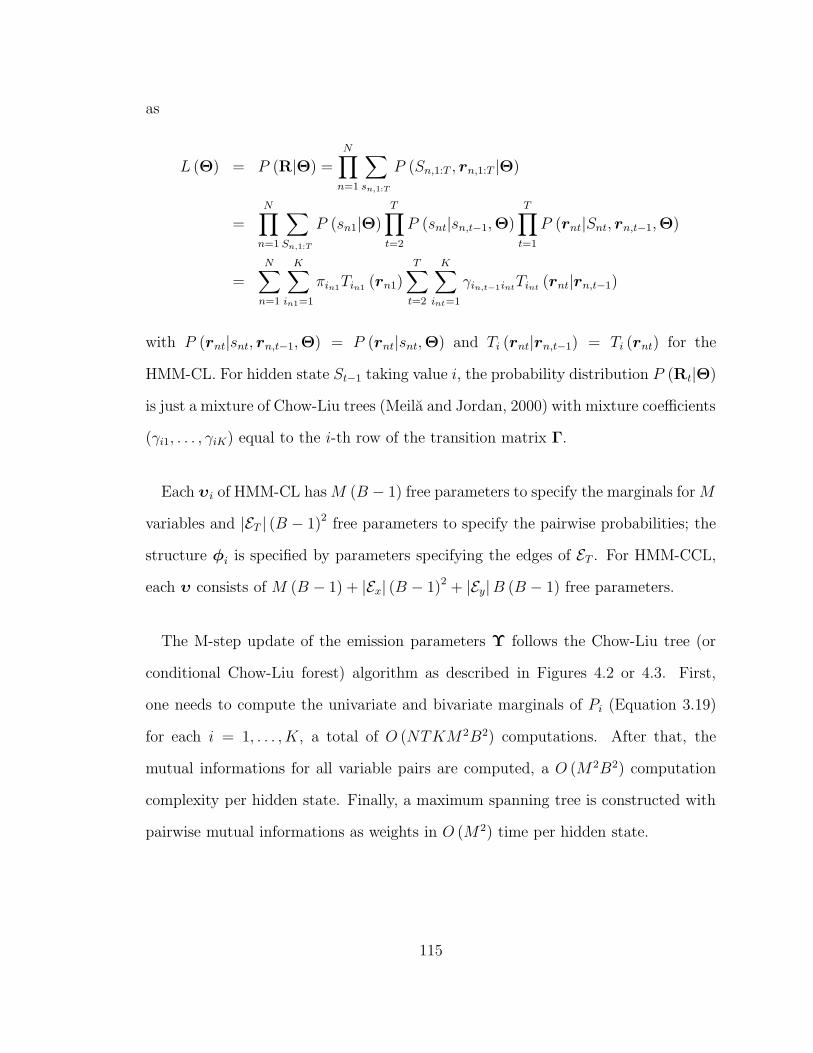
as

L (Θ) = P (R|Θ) =

N∏

n=1

∑

sn,1:T

P (Sn,1:T , rn,1:T |Θ)

=N∏

n=1

∑

Sn,1:T

P (sn1|Θ)T∏

t=2

P (snt|sn,t−1,Θ)T∏

t=1

P (rnt|Snt, rn,t−1,Θ)

=

N∑

n=1

K∑

in1=1

πin1Tin1 (rn1)

T∑

t=2

K∑

int=1

γin,t−1intTint

(rnt|rn,t−1)

with P (rnt|snt, rn,t−1,Θ) = P (rnt|snt,Θ) and Ti (rnt|rn,t−1) = Ti (rnt) for the

HMM-CL. For hidden state St−1 taking value i, the probability distribution P (Rt|Θ)

is just a mixture of Chow-Liu trees (Meila and Jordan, 2000) with mixture coefficients

(γi1, . . . , γiK) equal to the i-th row of the transition matrix Γ.

Each υi of HMM-CL has M (B − 1) free parameters to specify the marginals for M

variables and |ET | (B − 1)2 free parameters to specify the pairwise probabilities; the

structure φi is specified by parameters specifying the edges of ET . For HMM-CCL,

each υ consists of M (B − 1) + |Ex| (B − 1)2 + |Ey|B (B − 1) free parameters.

The M-step update of the emission parameters Υ follows the Chow-Liu tree (or

conditional Chow-Liu forest) algorithm as described in Figures 4.2 or 4.3. First,

one needs to compute the univariate and bivariate marginals of Pi (Equation 3.19)

for each i = 1, . . . , K, a total of O (NTKM 2B2) computations. After that, the

mutual informations for all variable pairs are computed, a O (M 2B2) computation

complexity per hidden state. Finally, a maximum spanning tree is constructed with

pairwise mutual informations as weights in O (M 2) time per hidden state.

115

6.2.1 HMM with Tree-Structured Normals

Similar to distributions for categorical data, we can combine HMMs with tree-

structured multivariate normal distributions, setting

p (rnt|Snt = i,Υ) = pNCL (rnt|µi,Σi) as defined in Section 5.2.2. This model, HMM-

CL-Normal, mirrors HMM-CL in structure (its Bayesian network structure class is

the same as for HMM-CL, Figure 6.1 (b)) and in parameter estimation. υi has

M + |ET | free parameters. The M-step emission update for HMM-CL-Normal is per-

formed following the steps of Figure 4.2. First, we estimate all univariate and bivari-

ate marginal distributions by computing µi and Ri for distributions Pi of Equation

3.19; this can be performed in O (NTKM 2) time. Mutual information estimation

does not require any computation since absolute values of correlations can be used

instead. A maximum spanning tree is obtained by Kruskal’s algorithm (e.g., Cormen

et al., 1990) in O (M 2) time per hidden state. Once the tree is obtained, the concen-

tration matrix entries needed for computation of p (rnt|snt) can be obtained in time

O (M) per hidden state.

6.3 HMM with Emission Models of Higher Com-

plexity

Both HMM-CL and HMM-CCL allow us to model some of the multivariate depen-

dency directly. However, the tree structure of the dependency model for the emissions

may be too restrictive. This is, perhaps, most pronounced in the HMM-CCL model

where emission distributions are broken into multiple independent tree-structured

components. We can use the maximum entropy models from Section 4.3 to relax the

structure restrictions.

116

6.3.1 HMM with Full Bivariate MaxEnt

We consider modeling P (rnt|Snt = i,Υ) as a full bivariate maximum entropy

model. For the binary case, the emission probability distributions can be expressed

as

P (rnt|Snt = i,Υ) =1

Cexp

(

M∑

j=1

αijrntj +

M∑

j=1

M∑

k=j+1

βijkrntjrntk

)

where C =∑

R

exp

(

M∑

j=1

αijrj +M∑

j=1

M∑

k=j+1

βijkrjrk

)

,

and υi = (αi1, . . . , αiM , βi12, . . . , βi,M−1,M) ∈ RM(M+1)/2.

We will call this model HMM-Full-MaxEnt. An example of a resulting Bayesian net-

work is shown in Figure 6.1 (c). This model has M (M + 1) /2 free parameters per

hidden state and captures all of the bivariate variable interactions, but at a signifi-

cant computational cost. In Section 4.3, we saw that the parameters of exponential

models are usually learned via iterative algorithms, and the full bivariate maximum

entropy model is no exception. Each update of υi in the M-step of each Baum-Welch

iteration would, in turn, be iterative. For small values of M , one can use iterative

scaling (IS) (e.g., Jelinek, 1998) to update υi. IS updates the parameters to match

the bivariate distributions of Pi (r) and P (r|υi). Bivariate marginals of Pi can be

precomputed in O (NTKMB2) time. However, the exact computation of each itera-

tion of IS is O(

2M−1)

,4 exponential in the dimensionality of the data vectors. There

are alternative techniques for parameter estimation of the full bivariate maximum en-

tropy distributions (e.g., sampling, belief propagation), all of them computationally

involved.

4Iterative scaling for full bivariate MaxEnt model requires computation of univariate and bivari-ate marginals at each iteration.

117

6.3.2 HMM with Saturated Normal Distributions

The real-valued Gaussian counterpart of the HMM-Full-MaxEnt is the HMM with

emission distributions modeled as normals with a full covariance matrix (Section

5.2.1):

p (rnt|Snt = i,Υ) = pN (rnt|µi,Σi) .

We denote this model HMM-Full-Normal. HMM-Full-Normal has the same graphical

model interpretation as HMM-Full-MaxEnt (Figure 6.1 (c)), and the same number of

free parameters, M (M + 1) /2 per hidden state. In contrast, the update of emission

parameters of HMM-Full-Normal can be done very efficiently, in only O (NTKM 2):

µi = EPi(R) =

∑Nn=1

∑Tt=1Ant (i) rnt

∑Nn=1

∑Tt=1 Ant (i)

and

Σi = V arPi(R) =

∑Nn=1

∑Tt=1 (r − µi) (r − µi)

′

∑Nn=1

∑Tt=1Ant (i)

.

Once the Σi are computed, the concentration matrices Ki needed for computation

of P (rnt|Snt = i,Υ) can be obtained in O (M 3) per hidden state.

6.3.3 HMM with Product of Univariate Conditional Max-

Ent Distributions

As we have seen in Section 4.3.2, we can use PUC-MaxEnt models to learn multi-

variate dependencies from data. Let V be the set of vertices corresponding to vector

variables at time t, and Vy be the set of vertices corresponding to vector variables at

118

time t− 1. Then

P (rnt|Snt = i,Υ) = PPUC−ME (rnt|δi,Fi)

where PPUC−ME (r) =∏

v∈V

1

Z(

rpa(v)

) exp

(

∑

f∈Fiv

δiff (r)

)

.

The structure parameters are the set of functions, φi = Fi. Coefficients δi are

the numeric parameters defining the distribution given the structure, i.e., υi = δi.

We will denote this HMM as HMM-PUC-MaxEnt. We can also similarly model

conditional probability distribution as P (rnt|rn,t−1, Snt = i,Υi) as a PUC-MaxEnt

model, following Equations 4.15 and 4.16:

P (rnt|rn,t−1, Snt = i,Υ) = PPUC−ME (rnt|rn,t−1, δi,Fi)

where PPUC−ME (r|r?) =∏

v∈V

1

Z(

rpax(v), r?pay(v)

) exp

(

∑

f∈Fiv

δiff (r, r?)

)

.

We will denote HMM with PUC-MaxEnt emissions by HMM-PUC-MaxEnt (Figure

6.1 (d)), and AR-HMM with PUC-MaxEnt emissions as AR-HMM-PUC-MaxEnt

(Figure 6.2 (c)).

We will concentrate on univariate and bivariate functions, as described in Section

4.3.5. Algorithm StructureLearningPUC-MaxEnt(Pi) (Figure 4.10) can be

used to update the parameters of the emission parameters at each M-step. To run

the algorithm, one does not require distributions Pi (r), just its bivariate marginals

obtainable in O (NTKM 2) time. Gains for candidate features can be computed in

O (NTM) time per iteration of Newton-Raphson, no more than O (M 2) computed

per iteration of the algorithm. Once a feature is added, each iteration of conjugate

gradient algorithm is performed in O (NTM) time as well. Since there are O (M 2)

119

possible pairwise interactions, no more than O (M 2) features will be added per hidden

state.

6.4 Summary

In this chapter, we introduced hidden Markov models for multivariate tempo-

ral data. The models vary (via the emission probabilities) in terms of the level of

multivariate interactions they encode, from conditional independence (no direct mul-

tivariate interactions) to maximum entropy models (possibly, all direct multivariate

interactions). However, the more complex the model gets, the higher (typically) the

computational complexity of the parameter estimation. Table 6.1 summarizes the

complexities of the models. The trade-off is especially evident for models for categor-

ical data with structures more complex than trees. For these models, the structure

and the numeric parameter learning cannot be performed simultaneously effectively

requiring inner loop iterations to search for the improved dependency structure.

There are a number of novel contributions in this chapter. HMM-CL and HMM-

CCL (Kirshner et al., 2004) offer efficient compromises between the quick but often

simplistic HMM-CI and the computationally intensive HMM-Full-MaxEnt. HMM-

PUC-MaxEnt and AR-HMM-PUC-MaxEnt allow to learn complex interactions be-

tween variables of Rnt given the hidden state. While both of the models are more

computationally demanding than simpler (HMM-CI, HMM-CL and HMM-CCL)

models, HMM-PUC-MaxEnt and AR-HMM-PUC-MaxEnt allow for richer depen-

dency structures, and their computational demands can be reduced by restricting

the complexity of the dependence structure.

120

In terms of related work, Zucchini and Guttorp (1991) explored the HMM-CI

model for precipitation occurrence modeling. As a follow-up, Hughes and Guttorp

(1994) introduced a non-homogeneous version of HMM-CI, and later described a

restricted non-homogeneous HMM-Full-MaxEnt model (Hughes et al., 1999). HMM-

CL and HMM-CCL models (Kirshner et al., 2004) introduce an aspect of learning

the dependence structure between data variables, not commonly seen in the HMM

framework. An exception is the work of Bilmes (1999, 2000) where HMMs are allowed

to learn temporal dependencies between individual output variables.

121

Table 6.1: Comparison of complexities of HMM models for multivariate time series

ModelComplexity ofP (r|rprev, s)

Complexity ofE-step

Complexity of M-step

HMM-CI O (M) O (NTK (K +M)) O (NTKMB)

HMM-Chains

O (M) O (NTK (K +M)) O (NTKMB2)

HMM-CLor HMM-

CCL

O (M) O (NTK (K +M)) O (NTKM2B2)

HMM-CL-Normal

O (M) O (NTK (K +M)) O (NTKM2)

HMM-Full-

MaxEnt

O (M2) O (NTK (K +M2)) O(

KI12M−1 +NTKM2

)

HMM-Full-

Normal

O (M2) O (NTK (K +M2)) O (NTKM2)

HMM-PUC-

MaxEnt orAR-HMM-

PUC-MaxEnt

O (M2) O (NTK (K +M2)) O (NTKM2 (I2M3 + I3M))

Comment: MaxEnt models are assumed binary with univariate or bivariate features.Legend: N – the number of sequences; T – the length of each sequence; K – thenumber of hidden states; M – the number of variables in the data vectors; B – thenumber of values each of the variables take; I1 – the number of iterations neededfor IS to converge; I2 – the number of iterations needed to compute Gain; I3 – thenumber of iterations needed for conjugate gradient algorithm to converge.

122

Chapter 7

Experimental Results: Sensitivity

of Learning HMMs for

Multivariate Binary Data

In this chapter we are addressing the question of the sensitivity of learning the

parameters of models from Chapter 6 for binary data with respect to the amount of

available data. We will demonstrate empirically the ability to learn both the numeric

and structural parameters given sufficient data, and we will also demonstrate that

these models may not recover the original parameters and structure if the amount of

training data is too small. We will also investigate whether a model can sufficiently

approximate another model with different structural properties.

The motivation for this kind of analysis comes from limited historical data available

for many applications. Assuming that we know the correct model type used to

generate the data, can we accurately learn the model parameters given the amount

of data that we have? For example, in the particular application of interest, are

123

24 sequences of 90 daily precipitation occurrence observations at 10 stations enough

data to learn the parameters of a 6-state HMM-CL accurately? We will perform an

empirical study in this chapter to answer this question.

7.1 Experimental Setup

The purpose of the experiment is to find out what amount of data is sufficient to

learn accurately the parameters of a model. Assume for the moment that the type

of the model is fixed and known, and that the set of true parameters of the model,

the target distribution, is known. We will simulate data sets of different sizes from

the target distribution and learn the parameters of the model from these sets. We

can then measure the differences between the learned distributions and the target

distribution.

We still need to define how to measure whether the learned distribution is simi-

lar enough to the target distribution. Since models for both the target and learned

distributions are the same, one possibility is a direct comparison of parameters.

The problem is the order in which emission distributions appear is not known, so a

consideration of all K! permutations of states may be necessary. Alternatively, we

could use one of the information theory measures of difference between distributions,

e.g., KL-divergence. The advantage is that such difference can be computed even

for distributions of different types, as long as they are defined on the same domain.

However, the KL-divergence between distributions with hidden variables usually can-

not be computed in closed form, and HMMs are no exception,1 although there are

1In order to define KL on HMMs, we need to specify the domain. We will assume that thedomain of distributions in question consists of all multivariate sequences of the same length T andthe same vector dimensionality M .

124

possible closed form approximations to KL for HMMs (e.g., Do, 2003). Instead of

using closed form approximations, we will approximate the exact values of the KL by

large sample approximation; we will generate a data set D = r1,1:T , . . . , rNKL,1:T

consisting of NKL sequences (where NKL is large) from target distribution P (r), and

then compute the difference in log-probability of the data under the target model

and the learned model Plearned:

KL (P ‖ Plearned) ≈ 1

NKL

NKL∑

n=1

(lnP (rn,1:T ) − lnPlearned (rn,1:T ))

=1

NKL

lnP (D) − 1

NKL

lnPlearned (D) . (7.1)

The first term on line 7.1 is an approximation of −HP [R], the negated entropy of

the target distribution. We can divide both terms by the number of observation

points in each sequence (T ×M) making the terms independent of the number of

observations (normalizing):

KLnorm (P ‖ Plearned) ≈1

NKLTMlnP (D) − 1

NKLTMlnPlearned (D) . (7.2)

For binary data, this normalized KL can be thought of as a relative entropy per

bit of data. We will call the log-likelihood terms on line 7.2 normalized or scaled

log-likelihoods. A model which assigns each binary observation a probability 0.5 (at

random) would have the scaled log-likelihood of − ln 2 ≈ −0.69315; we expect all of

the models trained on a data set to have scaled log-likelihoods higher than − ln 2.2

Then

0 ≤ KLnorm (P ‖ Plearned) ≤ −HP [R] + ln 2. (7.3)

2− ln 2 is a lower bound of the negative entropy for binary variables.

125

We perform the experiments under the following scheme. First, we choose types

of models to examine (from the models in Chapter 6). For each type, we consider a

range for K, the number of hidden states. For each combination of the model type

and the number of hidden states, we generate multiple sets of parameters (target

distributions) Θ1, . . . ,ΘNmfor the model. For each target distribution, we generate

10 sets of N sequences each of length T of M -dimensional binary (B = 2) vectors.

For each of such sets (with index is = 1, . . . , 10), we learn back the parameters

Θnis. To evaluate the models, we generate a large set from each original model with

NKL = 10000 and compute scaled log-likelihoods (and normalized KL-divergences)

of that set under the corresponding target model and all of the models approximating

that target model.

We perform two sets of experiments. With the first set, we investigate what factors

influence how well one can learn the parameters of an HMM given the correct model

type. We consider HMM-CI and HMM-CL with K = 2, . . . , 8 hidden states. First,

we generate Nm = 20 multiple sets of parameters per model type. We then generate

N = 10, 15, 20, 35, 50, 100, 200 sequences of binary vectors of dimensionality M = 15

for each parameter set, each sequence of length T = 100 (7 × 7 × 20 = 980 models

and 7 × 7 × 20 × 10 = 9800 sets of data for each type of the model). For each

simulated set, we learn back the parameters of the model using the same model

type used to generate that data set. We then evaluate the KL-divergence for each

learned set of parameters3. Since normalized KL-divergence depends on the entropy

of the target distribution (as the results in the next section suggest), we repeat

these experiments for three sets of parameters of target distributions with different

entropies. The average values of the entropies for the models used in this set of

3The settings of the EM algorithm used to estimate the parameters are discussed in AppendixC.

126

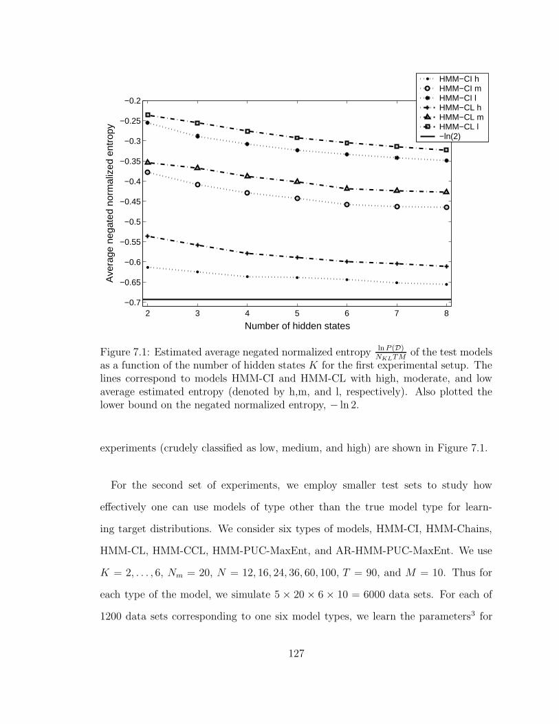
2 3 4 5 6 7 8−0.7

−0.65

−0.6

−0.55

−0.5

−0.45

−0.4

−0.35

−0.3

−0.25

−0.2

Number of hidden states

Ave

rage

neg

ated

nor

mal

ized

ent

ropy

HMM−CI hHMM−CI mHMM−CI lHMM−CL hHMM−CL mHMM−CL l−ln(2)

Figure 7.1: Estimated average negated normalized entropy ln P (D)NKLTM

of the test modelsas a function of the number of hidden states K for the first experimental setup. Thelines correspond to models HMM-CI and HMM-CL with high, moderate, and lowaverage estimated entropy (denoted by h,m, and l, respectively). Also plotted thelower bound on the negated normalized entropy, − ln 2.

experiments (crudely classified as low, medium, and high) are shown in Figure 7.1.

For the second set of experiments, we employ smaller test sets to study how

effectively one can use models of type other than the true model type for learn-

ing target distributions. We consider six types of models, HMM-CI, HMM-Chains,

HMM-CL, HMM-CCL, HMM-PUC-MaxEnt, and AR-HMM-PUC-MaxEnt. We use

K = 2, . . . , 6, Nm = 20, N = 12, 16, 24, 36, 60, 100, T = 90, and M = 10. Thus for

each type of the model, we simulate 5 × 20 × 6 × 10 = 6000 data sets. For each of

1200 data sets corresponding to one six model types, we learn the parameters3 for

127

all six model types with the same K as the true model.

7.2 Results

7.2.1 First Set of Experiments

First, we look at how close the scaled log-likelihoods of learned models approach

the scaled log-likelihoods of target distributions. Figure 7.2 summarizes the KL-

divergence for HMM-CI and HMM-CL models with target distributions having high,

moderate, and low entropies. Each of these plots show averaged scaled log-likelihood

for each number of hidden states K = 2, . . . , 8. From the figures it is apparent

that the learning algorithm can recover the target distribution given a sufficient

amount of data. Also, as expected, the accuracy of the learned model improves with

larger data sets. For the same amount of data, HMM-CI can recover the target

distribution with higher precision than HMM-CL; this is due to HMM-CL having

a higher number of free parameters. It appears that models with higher entropy of

the target distribution are estimated more accurately than same model types with

parameters yielding models with lower entropies. One possible naive explanation is

that if the original model has higher entropy, the learned models have a smaller range

of values for scaled log-likelihood and thus less room to be worse by a fixed margin.

For example, if the target distribution has scaled entropy of 0.65, the range of the

scaled KL-divergence is only [0, 0.0431] while a distribution with scaled entropy of

0.3 has its KL-divergence in the range of [0, 0.3931].

To quantify whether a data set of a certain size is sufficient for learning the param-

eters of the underlying (known) distribution for HMMs, we compute the empirical

probability that KLnorm (P ‖ Plearned) ≤ τ . We chose the value for the threshold

128

τ = 0.005.4 The probability can be computed based on 10× 20 values of KLnorm for

each value of K and N . If the probability is sufficiently high, we would consider the

amount of data sufficient. Figure 7.3 contains contour plots of the probabilities that

KLnorm ≤ τ for HMM-CI (left) and HMM-CCL (right) with high, moderate, and

low entropies. The x-axes are the number of free numeric parameters for the model

rather than the number K of hidden states. The y-axes are the total number of

binary points (in this case, 15×100 = 1500 times the number of sequences). Most of

the level curves are roughly linear on the log-scale. The implication is that we need

the log of the amount of data to be proportional to the number of free parameters to

be able to learn the parameters of the model with accuracy. Also, as the entropy of

the target distribution decreases, more data is needed to learn the model accurately

according to the same threshold τ .

4The value is decided on from looking at the parameter values for the models, but is subjectiveand somewhat arbitrary.

129

2 3 4 5 6 7 80

0.001

0.002

0.003

0.004

0.005

0.006

0.007

0.008

0.009

0.01


Ave

rage

nor

mal

ized

KL

1015203550100200

2 3 4 5 6 7 80

0.001

0.002

0.003

0.004

0.005

0.006

0.007

0.008

0.009

0.01


Ave

rage

nor

mal

ized

KL

1015203550100200

2 3 4 5 6 7 80

0.005

0.01

0.015


Ave

rage

nor

mal

ized

KL

1015203550100200

2 3 4 5 6 7 80

0.005

0.01

0.015

0.02

0.025

0.03

0.035

0.04

0.045


Ave

rage

nor

mal

ized

KL

1015203550100200

2 3 4 5 6 7 80

0.01

0.02

0.03

0.04

0.05

0.06


Ave

rage

nor

mal

ized

KL

1015203550100200

2 3 4 5 6 7 80

0.01

0.02

0.03

0.04

0.05

0.06

0.07

0.08

0.09


Ave

rage

nor

mal

ized

KL

1015203550100200

Figure 7.2: Estimated normalized KL-divergences for HMM-CI (top) and HMM-CL (bottom) with high (left), moderate (center), and low (right) average estimatedentropy as a function of the number of hidden states. Curves on each plot correspondto different values of the number of sequences N .

130

33 53 75 99 125 153 18315

22.5

30

52.5

75

150

300

Number of numeric parameters

Num

ber o

f bin

ary

obse

rvat

ions

(in

thou

sand

s)

0.050.20.35

0.5

0.5

0.65

0.65

0.8

0.8

0.95

0.95

61 95 131 169 209 251 29515

22.5

30

52.5

75

150

300


Num

ber o

f bin

ary

obse

rvat

ions

(in

thou

sand

s)

0.05

0.05

0.05

0.2

0.2

0.2

0.35

0.35

0.35

0.5

0.5

0.5

0.65

0.65

0.65

0.65

0.8

0.8

0.8

0.8

0.95

0.95

0.95

0.95

33 53 75 99 125 153 18315

22.5

30

52.5

75

150

300


Num

ber o

f bin

ary

obse

rvat

ions

(in

thou

sand

s)

0.050.20.2

0.35

0.35

0.5

0.5

0.65

0.65

0.65

0.8

0.8

0.8

0.95

0.95 0.95

0.95

61 95 131 169 209 251 29515

22.5

30

52.5

75

150

300


Num

ber o

f bin

ary

obse

rvat

ions

(in

thou

sand

s)

0.05

0.05

0.05

0.2

0.2

0.2

0.35

0.35

0.35

0.35

0.5

0.5

0.5

0.5

0.65

0.65

0.65

0.65

0.8

0.8

0.8

0.8

0.95

0.95

0.95

33 53 75 99 125 153 18315

22.5

30

52.5

75

150

300


Num

ber o

f bin

ary

obse

rvat

ions

(in

thou

sand

s)

0.050.2

0.2

0.35

0.35

0.5

0.5

0.65

0.65

0.65

0.8

0.8

0.8

0.95

0.95

0.95

0.95

61 95 131 169 209 251 29515

22.5

30

52.5

75

150

300


Num

ber o

f bin

ary

obse

rvat

ions

(in

thou

sand

s)

0.05

0.05

0.05

0.05

0.2

0.2

0.2

0.2

0.35

0.35

0.35

0.35

0.5

0.5

0.5

0.5

0.65

0.65

0.65

0.8

0.8

0.8

0.95

0.95

Figure 7.3: Contour plots of the probability that KLnorm ≤ τ (τ = 0.005) for HMM-CI (left) and HMM-CL (right) with high entropy (top), moderate entropy (center),and low entropy (bottom).

131

2 3 4 5 6 7 80.55

0.6

0.65

0.7

0.75

0.8

0.85

0.9

0.95


Pro

port

ion

of c

orre

ctly

lear

ned

edge

s

1015203550100200

2 3 4 5 6 7 80.55

0.6

0.65

0.7

0.75

0.8

0.85

0.9

0.95


Pro

port

ion

of c

orre

ctly

lear

ned

edge

s

1015203550100200

2 3 4 5 6 7 80.5

0.55

0.6

0.65

0.7

0.75

0.8

0.85

0.9


Pro

port

ion

of c

orre

ctly

lear

ned

edge

s

1015203550100200

Figure 7.4: Upper bounds on the proportion of correctly learned edges for HMM-CLwith high (left), moderate (center), and low (right) entropies as a function of thenumber of hidden states. Curves on each plot correspond to different values of thenumber of sequences N .

Finally, we examine whether HMM-CL can learn back the correct tree structure.

We wish to estimate what proportion of the tree edges in the original distribution

is recovered. To compute this number exactly, we need to match up the states of

the original and the learned models, an unrealistic task. Instead, we can compute

an upper bound to the proportion of recovered edges by lumping all of the edges

in each model together, and then computing the proportion of edges appearing in

both the original and the learned model. This upper bound on the proportion of

correctly learned edges is shown in Figure 7.4. As expected, the structure is learned

better when more data is available. Also, similar to observations from the estimated

KL-divergence, given the same amount of data, the structure of the distribution with

higher entropy can be learned more accurately than the one with the lower entropy.

132

7.2.2 Second Set of Experiments

First, we use the second experimental setup to extend the results in Figure 7.2

to other model types. The estimated values of KL-divergence for learned models

with the same type as the true model are shown Figure 7.5. All plots are consistent

with the intuition that more data will result in more accurate models. The plots

corresponding to HMM-CI (top left) and HMM-CL5 (top center) are consistent with

plots from the first experiment (Figure 7.2). Somewhat surprisingly, HMM-CCL

(bottom center) requires a little fewer data sequences than HMM-CL to learn back

the model parameters. Figure 7.6 further suggests this may be due in part to HMM-

CCL recovering the structure better than HMM-CL. Both HMM-PUC-MaxEnt (top

right) and AR-HMM-PUC-MaxEnt appear to hit a plateau in KL-divergence. This

may be due to the stopping criterion in the algorithm used to learn the feature sets

(Figure 4.10) as no feature adding less than certain improvement in log-likelihood is

added.

Finally, we consider how various models can approximate models of different types

of structure (no structure, multivariate, and temporal). We consider three types for

the true model: HMM-CI (no temporal or multivariate structure for hidden states),

HMM-CL (multivariate structure only), HMM-CCL (both multivariate and temporal

structure). For HMM-CI (Figure 7.7), any of the six HMM types can do a reasonable

job approximating it. However, models other than the true type (HMM-CI) tend to

overfit, especially the models that learn features. For HMM-CL (Figure 7.8), models

learning only the spatial structure, HMM-CL and HMM-PUC-MaxEnt, perform the

5This plot can provide an answer to the question in the beginning of this chapter. The plotsuggests that average KL-divergence for learning back the parameters of a 4-state HMM-CL is closeto 0.007, an acceptable number. However, as we have seen in the previous subsection, the entropyof the true model plays a significant part in a possible answer.

133

best. Models also learning the temporal structure perform reasonably but not as

well as HMM-CL or HMM-PUC-MaxEnt. HMM-CI and HMM-Chains are at a clear

disadvantage since they have no explicit mechanism to learn spatial dependencies.

For HMM-CCL (Figure 7.9), predictably, AR-HMM-PUC-MaxEnt does the best job

(after HMM-CCL) as it can learn both spatial and temporal features. The rest of

the models perform poorly since they cannot model additional temporal or spatial

information.

7.3 Summary

In this chapter, we have shown empirically that HMM-CI, HMM-CL, and HMM-

CCL (both parameters and structures) can be learned accurately given sufficient

data. We defined a measure of accuracy in learning the parameters, and studied how

accurately can the parameters of a multivariate HMM be learned as a function of

the data set size. The empirical plots suggest that the size of the data set needed for

accurate parameter estimation depends not only on the number of free parameters,

but also on the entropy of the target distribution. The experiments also suggest that

models capable of learning the same types of features, spatial and/or temporal, as the

true model can be used as a good approximation although with a risk of overfitting.

134

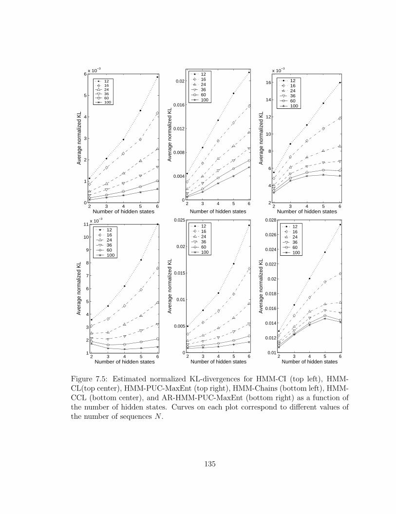
2 3 4 5 60

1

2

3

4

5

6x 10

−3


Ave

rage

nor

mal

ized

KL

1216243660100

2 3 4 5 60

0.004

0.008

0.012

0.016

0.02


Ave

rage

nor

mal

ized

KL

1216243660100

2 3 4 5 62

4

6

8

10

12

14

16

x 10−3


Ave

rage

nor

mal

ized

KL

1216243660100

2 3 4 5 61

2

3

4

5

6

7

8

9

10

11x 10

−3


Ave

rage

nor

mal

ized

KL

1216243660100

2 3 4 5 60

0.005

0.01

0.015

0.02

0.025


Ave

rage

nor

mal

ized

KL

1216243660100

2 3 4 5 60.01

0.012

0.014

0.016

0.018

0.02

0.022

0.024

0.026

0.028


Ave

rage

nor

mal

ized

KL

1216243660100

Figure 7.5: Estimated normalized KL-divergences for HMM-CI (top left), HMM-CL(top center), HMM-PUC-MaxEnt (top right), HMM-Chains (bottom left), HMM-CCL (bottom center), and AR-HMM-PUC-MaxEnt (bottom right) as a function ofthe number of hidden states. Curves on each plot correspond to different values ofthe number of sequences N .

135

2 3 4 5 60.55

0.6

0.65

0.7

0.75

0.8

0.85

0.9

0.95


Pro

port

ion

of c

orre

ctly

lear

ned

edge

s

1216243660100

2 3 4 5 60.55

0.6

0.65

0.7

0.75

0.8

0.85

0.9

0.95


Pro

port

ion

of c

orre

ctly

lear

ned

edge

s

1216243660100

Figure 7.6: Upper bounds on the proportion of correctly learned edges for HMM-CL(left) and HMM-CCL (right) as a function of the number of hidden states. Curveson each plot correspond to different values of the number of sequences N .

2 3 4 5 60

0.001

0.002

0.003

0.004

0.005

0.006

0.007

0.008

0.009

0.01


Ave

rage

nor

mal

ized

KL

HMM−CIHMM−ChainsHMM−CLHMM−CCLHMM−PUC−MaxEntAR−HMM−PUC−MaxEnt

2 3 4 5 60

0.5

1

1.5

2

2.5

3x 10

−3


Ave

rage

nor

mal

ized

KL


Figure 7.7: Estimated normalized KL-divergences for different models for estimationthe parameters of a HMM-CI based on 24 sequences (left) and 100 sequences (right).Curves on each plot correspond to different models.

136

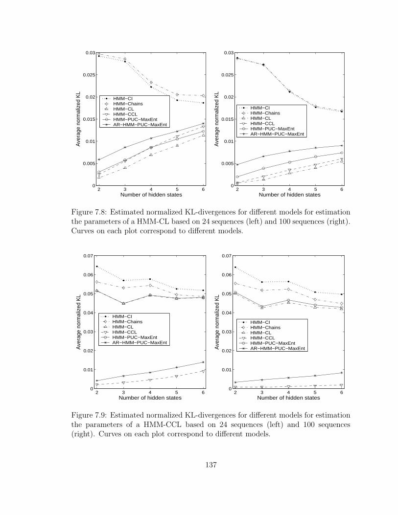
2 3 4 5 60

0.005

0.01

0.015

0.02

0.025

0.03


Ave

rage

nor

mal

ized

KL


2 3 4 5 60

0.005

0.01

0.015

0.02

0.025

0.03


Ave

rage

nor

mal

ized

KL


Figure 7.8: Estimated normalized KL-divergences for different models for estimationthe parameters of a HMM-CL based on 24 sequences (left) and 100 sequences (right).Curves on each plot correspond to different models.

2 3 4 5 60

0.01

0.02

0.03

0.04

0.05

0.06

0.07


Ave

rage

nor

mal

ized

KL


2 3 4 5 60

0.01

0.02

0.03

0.04

0.05

0.06

0.07


Ave

rage

nor

mal

ized

KL


Figure 7.9: Estimated normalized KL-divergences for different models for estimationthe parameters of a HMM-CCL based on 24 sequences (left) and 100 sequences(right). Curves on each plot correspond to different models.

137

Chapter 8

Experimental Results: Large Scale

Study of Precipitation Modeling

for Different Geographic Regions

In this chapter, we apply the methodology developed in Chapters 3-6 to the prob-

lem of modeling daily precipitation occurrence simultaneously at multiple rain sta-

tions for different geographic regions. First, we briefly summarize prior statistical

work for this application (Section 8.1). Then, we describe the analysis methodology

(Section 8.2). After that, we consider four different geographic regions with different

amounts of data (Section 8.3). For each region, we summarize the data, compare the

performance of the models on the data, and consider possible interpretation of the

weather states.

138

8.1 Related Work on Multi-site Precipitation Oc-

currence Modeling

Statistical approaches to precipitation occurrence modeling date back to the 1850’s

(Katz, 1985). However, until recently, most of the work concentrated on modeling

data collected from a single weather station. Wilks and Wilby (1999) provide an

overview of the literature related to early stochastic precipitation modeling. Most

of the described methods model rainfall occurrence as a Markov chain with two

states, wet and dry, sometimes using higher order Markov chains. The run-lengths

of wet and dry spells commonly exhibit near-geometric distributions. Thus, 2-state

Markov chains can often be used to simulate data with run-lengths matching that of

the historical data. However, these single-station models cannot be easily extended

to multiple sites as that requires modeling multivariate (or spatial) dependencies

between the stations. Using an unconstrained Markov chain on the vector of occur-

rences is impractical since the number of parameters required is exponential in the

number of stations (Guttorp, 1995). Wilks (1998) used multivariate probit models to

match the pairwise correlations of daily observations, and later extended the method

to capture some of the climate variability by allowing seasonal atmospheric variables

to influence the parameters of the model (Wilks, 2002). Alternatively, a mathemat-

ical model of the spatial physical process can be used to simulate precipitation at

multiple locations (e.g., Waymire et al., 1984; Goodall and Phelan, 1991; Cox and

Isham, 1988). Yet another alternative is to model multi-site precipitation dependent

only on the finite number of evolving weather states with states either being explicitly

classified based on the atmospheric conditions (e.g., Hay et al., 1991; Wilson et al.,

1992; Bardossy and Plate, 1992) or considered unobserved, the latter resulting in an

HMM. Other alternatives include non-parametric methods, for example, k-nearest

139

neighbor algorithm (Rajagopalan and Lall, 1999), or modeling station dependence

via a Bayesian network (Cofino et al., 2002).1 In some cases, the weather states are

not assumed to be discrete (e.g., Sanso and Guenni, 1999), and can even be viewed

as an evolving random field (Allcroft and Glasbey, 2003).

Hidden Markov models have been successfully applied to multi-site precipitation

modeling since they were introduced by Zucchini and Guttorp (1991). Hughes and

Guttorp (1994) extended the HMM framework to allow the weather states to evolve

dependent on the atmospheric variables. Initially, the occurrences were modeled

conditionally independent given the states, but later models remove this restriction

(Hughes et al., 1999). It is worth noting that the HMM framework can be easily

extended to model multi-site rainfall amounts as well (e.g., Bellone, 2000; Bellone

et al., 2000).

Precipitation modeling has a number of potential uses in water management and

forecasting. (See, for example, Wilks and Wilby, 1999, for more information.) Simu-

lated precipitation data sequences can be used to study interannual climate variability

and possibly be used in forecasting. These simulated sequences can also be used as

inputs in crop models. Historical records for a number of geographic regions (e.g.,

Kenya, India) contain a large quantity of missing data presenting a serious problem

for analysis and forecasting. Stochastic precipitation models could alleviate some of

the problems by estimating or simulating these missing values.

1Bellone (2000) contains an excellent review of the development of statistical methods for pre-cipitation modeling.

140

8.2 Model Selection and Evaluation of the Results

As was mentioned in Chapter 1, we want to develop generative models (based

on the historical data) that can produce realistic simulated daily rainfall occurrence

sequences for networks of stations. Before analyzing possible models, we need to

decide how to evaluate the models and what criteria to use to choose between mod-

els. We employ leave-k-out cross-validation for model selection. Assume we have

a set of N ordered data sequences (typically these correspond to daily sequences

for N different years or seasons). Under leave-k-out cross-validation, we will train

N/k models, one for each set obtained by leaving-out k non-overlapping consecutive

sequences. Each model is then evaluated on the corresponding left-out k sequences.

For evaluation criteria, we use a mix of statistics capturing temporal, spatial, and

interannual variability properties of the data, as well as the fit of the model to the

data, and the ability of the model to fill-in missing observations. Possible criteria

include the difference in linear correlation for observed and simulated data, the dif-

ference in probability of precipitation at a given station for observed and simulated

data, the difference in precipitation persistence (as explained later) for observed and

simulated data, the scaled log-likelihood of the left-out sequences (Chapter 7), and

the average classification error in predicting randomly-selected observations that are

deliberately removed from the left-out data and then predicted by the model. Per-

sistence is defined as the probability of a precipitation occurrence for a particular

station given precipitation event at that station at previous observation. Persistence

can be thought of as a proxy for wet spell run-length distributions (Chapter 1) as

these spells can often be modeled by a geometric distribution with one free param-

eter. Average classification error helps in assessing whether the model can remedy

the common situation of missing station readings in real precipitation records.

141

The parameters for individual hidden states of fitted HMMs can often be visu-

alized (as will be shown in the next section), and these sometimes called “weather

states” are often of direct scientific interest from a meteorological viewpoint. Thus,

in evaluating these models, models that can explain the data with fewer states are

generally preferable.

8.3 Performance Analysis on Geographic Regions

We use the models described earlier in the thesis to analyze four data sets, each

for a distinct geographic region: Ceara region of Northeastern Brazil, Southwestern

Australia, Western U.S., and Queensland region of Northeastern Australia. The

exact setup for the experiments can be found in Appendix C. Some of the analysis

from Subsections 8.3.2 and 8.3.3 appeared in Kirshner et al. (2004).

8.3.1 Ceara Region of Northeastern Brazil

First, we model the data for the Ceara region. (The set was described in detail

in Section 1.1.) We will use leave-one-out and leave-six-out cross-validations for the

Ceara set. By leaving out only one data sequence at a time, we evaluate models

trained on sets almost identical to the whole set, and get an accurate estimate for

the average out-of-sample log-likelihood, an indicator of the predictive power of the

model. However, this method is computationally intensive (as it requires almost N

times the computation of an algorithm run on the whole data). Also, one-sequence

validation sets are too small to evaluate the correlation and the persistence as these

statistics have high variance for individual years (as illustrated for persistence in

Figure 8.1), so larger validation sets are desirable. However, since the data set is

already small, leaving out large number of seasons will leave too little data to train

142

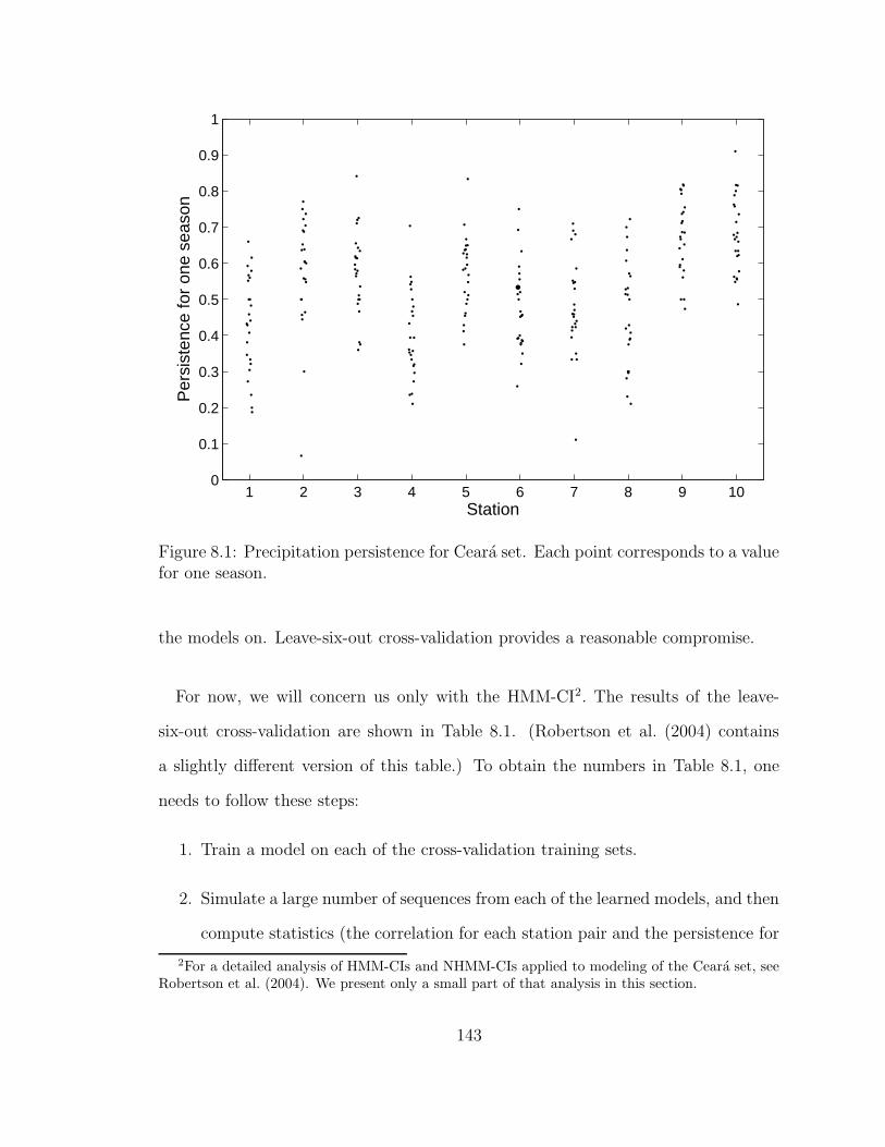
1 2 3 4 5 6 7 8 9 100

0.1

0.2

0.3

0.4

0.5

0.6

0.7

0.8

0.9

1

Station

Per

sist

ence

for

one

seas

on

Figure 8.1: Precipitation persistence for Ceara set. Each point corresponds to a valuefor one season.

the models on. Leave-six-out cross-validation provides a reasonable compromise.

For now, we will concern us only with the HMM-CI2. The results of the leave-

six-out cross-validation are shown in Table 8.1. (Robertson et al. (2004) contains

a slightly different version of this table.) To obtain the numbers in Table 8.1, one

needs to follow these steps:

1. Train a model on each of the cross-validation training sets.

2. Simulate a large number of sequences from each of the learned models, and then

compute statistics (the correlation for each station pair and the persistence for

2For a detailed analysis of HMM-CIs and NHMM-CIs applied to modeling of the Ceara set, seeRobertson et al. (2004). We present only a small part of that analysis in this section.

143

each station) for each simulated set.

3. For each of the left-out sets (as determined by cross-validation):

• Compute the correlation and the persistence; compute the absolute differ-

ence between these statistics and the same statistics of the corresponding

simulated data.

• Compute the scaled log-likelihood (of the corresponding model) and the

average classification error of prediction by leaving out a single observation

and then predicting it with the corresponding model.

4. Average the results across the data sets.

A K-state M -variate binary HMM-CI has K2 − 1 + M ∗ K free parameters, K2 +

10K − 1 for this set. There is no clear improvement in numbers for K > 4, so the

numbers suggest training the model with K = 4. The numbers for the out-of-sample

evaluation for the leave-one-out cross-validation (Table 8.2) are a little better than

their counterparts for the leave-six-out cross-validation case. More accurate models

are the result of training on the 23 sequences (versus 18 with leave-six-out cross-

validation). Again, however, there is no significant improvement past K = 4, so

both cross-validations point to the same conclusion for K.

By overimposing the probabilities of precipitation for each station in each hidden

state over the map of the region, we can visualize the resulting hidden (weather)

states. Figure 8.4 shows these states for 4-state HMM-CI trained on all 24 data

sequences. The transition probabilities for this 4-state model are provided in Table

8.3. The transition matrix suggests that both the “wet” state (state 1) and the “dry”

state (state 2) are somewhat persistent as indicated by values of corresponding self-

transition parameters. The transitions between these two states occur mostly through

144

2 3 4 5 6 7 8−0.59

−0.585

−0.58

−0.575

−0.57

−0.565

−0.56


Ave

rage

sca

led

log−

likel

ihoo

d

HMM−CIHMM−ChainsHMM−CLHMM−CCLHMM−MaxEntHMM−PUC−MaxEntAR−HMM−PUC−MaxEnt

Figure 8.2: Ceara data: average out-of-sample log-likelihood obtained by a leave-one-out cross-validation for various models across a number of hidden states.

the other two “transitional” states with state 3 occurring more frequently than state

4 (Robertson et al., 2004).

Figure 8.2 compares the average out-of-sample log-likelihoods for different mod-

els under leave-one-out cross-validation. Figure 8.3 compares the expected accuracy

of correlation (top) and persistence (bottom) according to the leave-six-out cross-

validation. The measurements are quite noisy as training sets are small, especially

for models with large numbers of parameters (e.g., AR-HMM-PUC-MaxEnt, mod-

els with large numbers of hidden states). For all models, except for HMM-CI, no

significant improvement is noticeable for K > 3. According to the log-likelihood,

145

HMM-MaxEnt clearly overfits3 while the rest of the models have comparable perfor-

mances, with HMM-CI requiring larger number of hidden states to match the per-

formance of other models. As expected, the models with spatial structure perform

the best according to the difference in correlation while the models with temporal

structure perform the best according to the difference in persistence. Thus, HMM-

CCL or AR-HMM-PUC-MaxEnt with K = 3 hidden states would provide a solution

with good performance according to the statistics of interest. However, even without

temporal links between the stations, HMMs can capture statistics of the data; the

data simulated from a 3-state HMM-CL and a 4-state HMM-CI models trained on

all 24 years of the data has statistics resembling the original data set. Probabilities

of precipitation for individual stations obtained from the data simulated from either

of 4-state HMM-CI or 3-state HMM-CL match the corresponding probabilities for

the historical data exactly (Figure 8.6 left). Between-station correlations are also

quite closely matched, especially for 3-state HMM-CL (Figure 8.5). However, the

persistence numbers are somewhat underestimated (Figure 8.6 right) leading to an

underestimation of lengths of the wet spells.

3This is not surprising since HMM-MaxEnt requires M (M − 1) /2 free parameters per hiddenstate. Hughes et al. (1999) suggest reducing the number of free parameters by parametrizing themusing the geo-locations of the stations.

146

Table 8.1: Performance of HMM-CIs evaluated by leave-six-out cross-validation.

Averageout-of-sample Average

Average absolute out-of-sample AverageNumber out-of-sample difference absolute out-of-sampleof hidden scaled in correlation (over difference classification

states log-likelihood all stations pairs) in persistence accuracyK = 2 −0.5855 0.0622 0.0796 69.22K = 3 −0.5742 0.0516 0.0682 71.26K = 4 −0.5709 0.0464 0.0643 71.53K = 5 −0.5683 0.0461 0.0650 71.75K = 6 −0.5685 0.0453 0.0645 71.96K = 7 −0.5697 0.0447 0.0644 71.71K = 8 −0.5699 0.0438 0.0632 71.85

Table 8.2: Performance of HMM-CIs evaluated by leave-one-out cross-validation.

Number Number Average Averageof hidden of free out-of-sample out-of-sample

states parameters scaled log-likelihood classification accuracyK = 2 23 −0.5834 69.15K = 3 38 −0.5712 71.71K = 4 55 −0.5672 71.96K = 5 74 −0.5659 72.09K = 6 95 −0.5646 72.38K = 7 118 −0.5643 72.46K = 8 143 −0.5662 71.94

Table 8.3: Transition parameters for 4-state HMM-CI trained on Ceara data.

ToFrom

State 1 State 2 State 3 State 4State 1 0.6988 0.0115 0.1652 0.1245State 2 0.0238 0.6824 0.1583 0.1355State 3 0.1570 0.1451 0.5884 0.1095State 4 0.2352 0.1918 0.1602 0.4128

147

2 3 4 5 6 7 80.04

0.045

0.05

0.055

0.06

0.065


Ave

rage

abs

olut

e di

ffere

nce

in c

orre

latio

n


2 3 4 5 6 7 80.06

0.065

0.07

0.075

0.08

0.085


Ave

rage

abs

olut

e di

ffere

nce

in p

ersi

sten

ce


Figure 8.3: Ceara data: average out-of-sample absolute difference between the statis-tics of the simulated data and the left-out data as determined by leave-six-out cross-validation for correlation (top) and persistence (bottom).

148

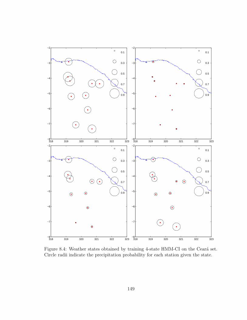
318 319 320 321 322 323−8

−7

−6

−5

−4

−3

−2

0.1

0.3

0.5

0.7

0.9

318 319 320 321 322 323−8

−7

−6

−5

−4

−3

−2

0.1

0.3

0.5

0.7

0.9

318 319 320 321 322 323−8

−7

−6

−5

−4

−3

−2

0.1

0.3

0.5

0.7

0.9

318 319 320 321 322 323−8

−7

−6

−5

−4

−3

−2

0.1

0.3

0.5

0.7

0.9

Figure 8.4: Weather states obtained by training 4-state HMM-CI on the Ceara set.Circle radii indicate the precipitation probability for each station given the state.

149

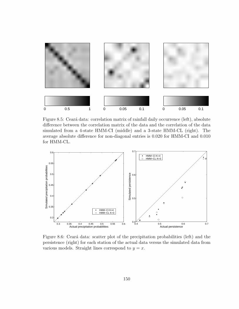
0 0.5 1 0 0.05 0.1 0 0.05 0.1

Figure 8.5: Ceara data: correlation matrix of rainfall daily occurrence (left), absolutedifference between the correlation matrix of the data and the correlation of the datasimulated from a 4-state HMM-CI (middle) and a 3-state HMM-CL (right). Theaverage absolute difference for non-diagonal entries is 0.020 for HMM-CI and 0.010for HMM-CL.

0.3 0.35 0.4 0.45 0.5 0.55 0.6

0.3

0.35

0.4

0.45

0.5

0.55

0.6

Actual precipitation probabilities

Sim

ulat

ed p

reci

pita

tion

prob

abili

ties

HMM−CI K=4HMM−CL K=3

0.4 0.5 0.6 0.70.4

0.5

0.6

0.7

Actual persistence

Sim

ulat

ed p

ersi

sten

ce

HMM−CI K=4HMM−CL K=3

Figure 8.6: Ceara data: scatter plot of the precipitation probabilities (left) and thepersistence (right) for each station of the actual data versus the simulated data fromvarious models. Straight lines correspond to y = x.

150

115 116 117 118 119

−35

−34

−33

−32

−31

−30

=90%

=50%

=10%

Figure 8.7: Stations in the Southwestern Australia region. Circle radii indicatemarginal probabilities of rainfall (> 0.3mm) at each location.

8.3.2 Southwestern Australia

In the experiments below we use data collected from 30 stations over 15 184-day

winter seasons (May–October, 1978–1992).4 Figure 8.7 shows the network of stations.

We use leave-one-out cross-validation to evaluate the predictive accuracy of the

models on this data set. For evaluation, we use two different criteria. We compute the

scaled log-likelihood and the average classification error for seasons not in the training

data. The models considered are the HMM with conditional independence (HMM-

CI), the HMM with dependence on the previous observation for the same station

4This data has been collected by the Commonwealth Bureau of Meteorology of Australia andprovided to us by Dr. Stephen P. Charles of CSIRO (Commonwealth Scientific and IndustrialResearch Organisation) Land and Water, Australia.

151

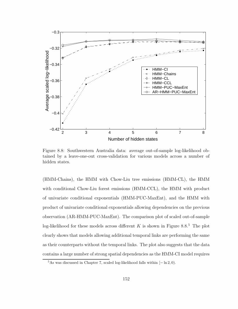
2 3 4 5 6 7 8−0.42

−0.4

−0.38

−0.36

−0.34

−0.32

−0.3


Ave

rage

sca

led

log−

likel

ihoo

d


Figure 8.8: Southwestern Australia data: average out-of-sample log-likelihood ob-tained by a leave-one-out cross-validation for various models across a number ofhidden states.

(HMM-Chains), the HMM with Chow-Liu tree emissions (HMM-CL), the HMM

with conditional Chow-Liu forest emissions (HMM-CCL), the HMM with product

of univariate conditional exponentials (HMM-PUC-MaxEnt), and the HMM with

product of univariate conditional exponentials allowing dependencies on the previous

observation (AR-HMM-PUC-MaxEnt). The comparison plot of scaled out-of-sample

log-likelihood for these models across different K is shown in Figure 8.8.5 The plot

clearly shows that models allowing additional temporal links are performing the same

as their counterparts without the temporal links. The plot also suggests that the data

contains a large number of strong spatial dependencies as the HMM-CI model requires

5As was discussed in Chapter 7, scaled log-likelihood falls within [− ln 2, 0).

152

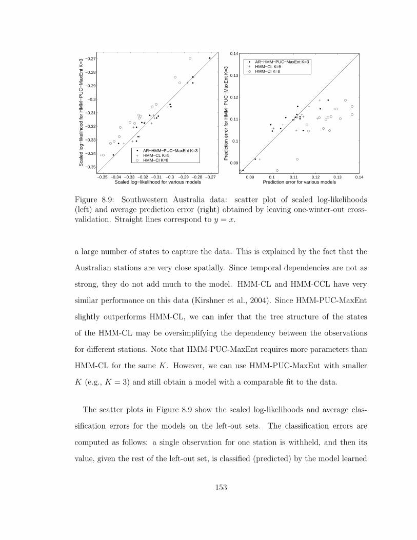
−0.35 −0.34 −0.33 −0.32 −0.31 −0.3 −0.29 −0.28 −0.27

−0.35

−0.34

−0.33

−0.32

−0.31

−0.3

−0.29

−0.28

−0.27

Scaled log−likelihood for various models

Sca

led

log−

likel

ihoo

d fo

r H

MM

−P

UC

−M

axE

nt K

=3

AR−HMM−PUC−MaxEnt K=3HMM−CL K=5HMM−CI K=8

0.09 0.1 0.11 0.12 0.13 0.14

0.09

0.1

0.11

0.12

0.13

0.14

Prediction error for various models

Pre

dict

ion

erro

r fo

r H

MM

−P

UC

−M

axE

nt K

=3

AR−HMM−PUC−MaxEnt K=3HMM−CL K=5HMM−CI K=8

Figure 8.9: Southwestern Australia data: scatter plot of scaled log-likelihoods(left) and average prediction error (right) obtained by leaving one-winter-out cross-validation. Straight lines correspond to y = x.

a large number of states to capture the data. This is explained by the fact that the

Australian stations are very close spatially. Since temporal dependencies are not as

strong, they do not add much to the model. HMM-CL and HMM-CCL have very

similar performance on this data (Kirshner et al., 2004). Since HMM-PUC-MaxEnt

slightly outperforms HMM-CL, we can infer that the tree structure of the states

of the HMM-CL may be oversimplifying the dependency between the observations

for different stations. Note that HMM-PUC-MaxEnt requires more parameters than

HMM-CL for the same K. However, we can use HMM-PUC-MaxEnt with smaller

K (e.g., K = 3) and still obtain a model with a comparable fit to the data.

The scatter plots in Figure 8.9 show the scaled log-likelihoods and average clas-

sification errors for the models on the left-out sets. The classification errors are

computed as follows: a single observation for one station is withheld, and then its

value, given the rest of the left-out set, is classified (predicted) by the model learned

153

on the training test; the error is then averaged over all observations in the hold-out

set. K is chosen subjectively according to the scaled log-likelihood for each model as

we want to select a model providing a good fit with the smallest number of hidden

states. The y-axis is the performance of the HMM-PUC-MaxEnt model, and the x-

axis represents the performance of the other models (shown with different symbols).

Higher implies better performance for log-likelihood (on the left) and worse for error

(on the right). A 3-state HMM-PUC-MaxEnt (249 free real-valued parameters67) is

performing about as well as both a 3-state AR-HMM-PUC-MaxEnt (279 free real-

valued parameters87) and a 5-state HMM-CL (319 free real-valued parameters6), and

noticeably better than an 8-state HMM-CI (303 free parameters). The statistics of

the data simulated from such model (3-state HMM-PUC-MaxEnt) trained on all 15

seasons of data resemble that of the actual data (Figures 8.10 and 8.11), with exact

match for precipitation occurrence probabilities, good match for correlations, and a

slight underestimation of rainfall persistence.

Examples of the Chow-Liu tree structures learned by the model are shown in Fig-

ure 8.12 for the 5-state HMM-CL model trained on all 15 years of Southwestern

Australia data. The states learned by the model correspond to a variety of wet and

dry spatial patterns. The tree structures are consistent with the meteorology and

topography of the region (Hughes et al., 1999). Winter rainfall over SW Australia is

large-scale and frontal, impacting the southwest corner of the domain first and fore-

most. Hence, the tendency for correlations between stations along the coast during

moderately wet weather states. Interesting correlation structures are also identified

6This number does not include the parameters need to specify the features.7Number of parameters is for the model with the highest log-likelihood trained on the set with

all data sequences.8This number does not include the parameters needed to specify the features and the parameters

needed to specify the probabilities for the first observation in each sequence.

154

in the north of the domain even during dry conditions. For comparison, we consider

other HMMs not modeling additional time dependencies, HMM-CI and HMM-PUC-

MaxEnt, with weather states shown in Figures 8.13 and 8.14, respectively. All three

models have easily identifiable wet (top left) and dry (bottom) states with the same

rainfall probabilities for individual stations across the models in these states. HMM-

CL and HMM-PUC-MaxEnt have very similar stations’ precipitation probabilities

for the other three states; the edge structures also exhibit similarities. On the other

hand, HMM-CI’s other weather states do not match well to states of either HMM-CL

or HMM-PUC-MaxEnt. HMM-CCL’s weather states (Figure 8.15) differ very little

from states of HMM-CL in stations’ precipitation and mildly in spatial edges with

very few temporal edges present in HMM-CCL; this indicates that the dependence

in the data is mostly spatial.

155

0 0.02 0.04 0.06 0.08 0.10 0.2 0.4 0.6 0.8 1

Figure 8.10: Southwestern Australia data: correlation matrix of rainfall daily occur-rence (left), absolute difference between the correlation matrix of the data and thecorrelation of the data simulated from a 3-state HMM-PUC-MaxEnt (right). Theaverage absolute difference for non-diagonal entries is 0.025.

0.25 0.3 0.35 0.4 0.45 0.5 0.55 0.6 0.65

0.25

0.3

0.35

0.4

0.45

0.5

0.55

0.6

0.65


Sim

ulat

ed p

reci

pita

tion

prob

abili

ties

HMM−PUC−MaxEnt K=3

0.4 0.5 0.6 0.7 0.80.35

0.4

0.45

0.5

0.55

0.6

0.65

0.7

0.75

0.8

Actual persistence

Sim

ulat

ed p

ersi

sten

ce

HMM−PUC−MaxEnt K=3

Figure 8.11: Southwestern Australia data: scatter plot of the precipitation probabil-ities (left) and the persistence (right) for each station of the actual data versus thesimulated data from various models. Straight lines correspond to y = x.

156

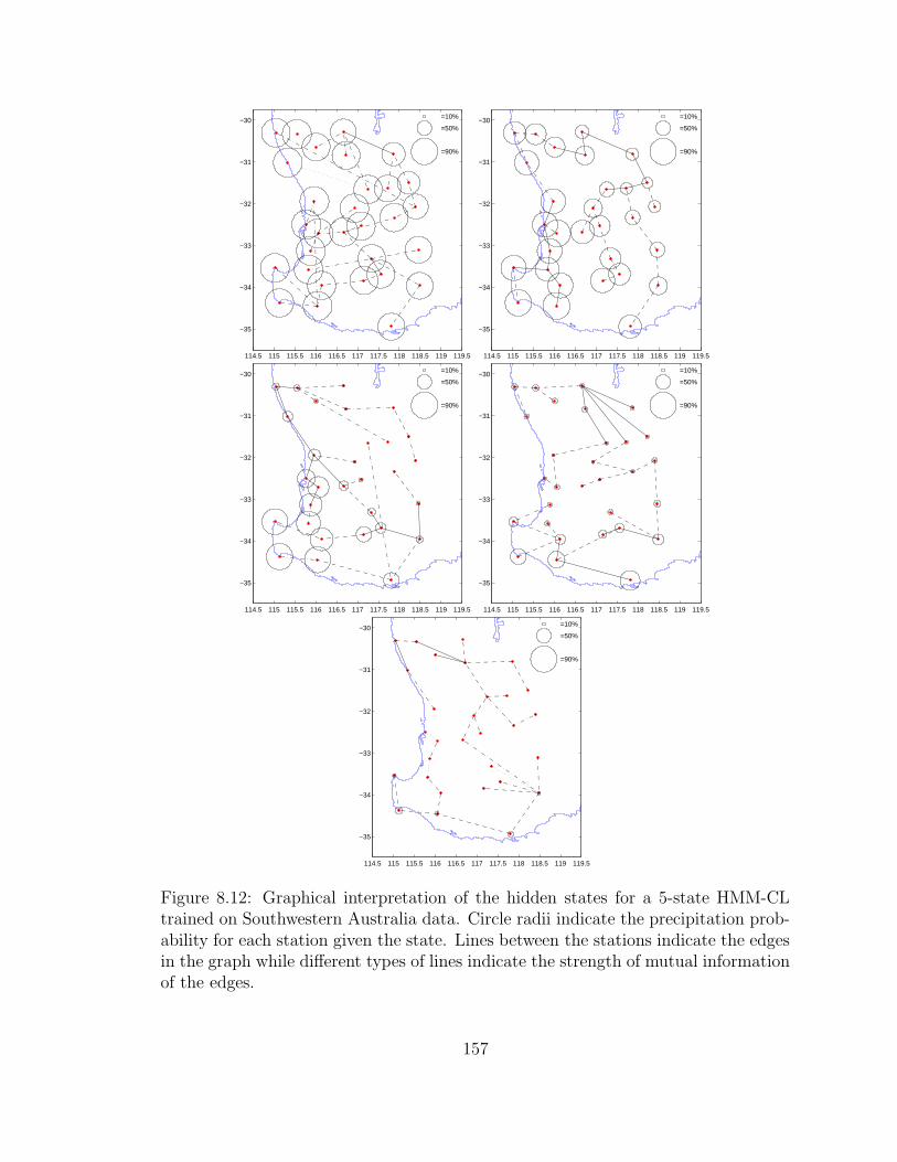
114.5 115 115.5 116 116.5 117 117.5 118 118.5 119 119.5

−35

−34

−33

−32

−31

−30

=90%

=50%

=10%

114.5 115 115.5 116 116.5 117 117.5 118 118.5 119 119.5

−35

−34

−33

−32

−31

−30

=90%

=50%

=10%

114.5 115 115.5 116 116.5 117 117.5 118 118.5 119 119.5

−35

−34

−33

−32

−31

−30

=90%

=50%

=10%

114.5 115 115.5 116 116.5 117 117.5 118 118.5 119 119.5

−35

−34

−33

−32

−31

−30

=90%

=50%

=10%

114.5 115 115.5 116 116.5 117 117.5 118 118.5 119 119.5

−35

−34

−33

−32

−31

−30

=90%

=50%

=10%

Figure 8.12: Graphical interpretation of the hidden states for a 5-state HMM-CLtrained on Southwestern Australia data. Circle radii indicate the precipitation prob-ability for each station given the state. Lines between the stations indicate the edgesin the graph while different types of lines indicate the strength of mutual informationof the edges.

157

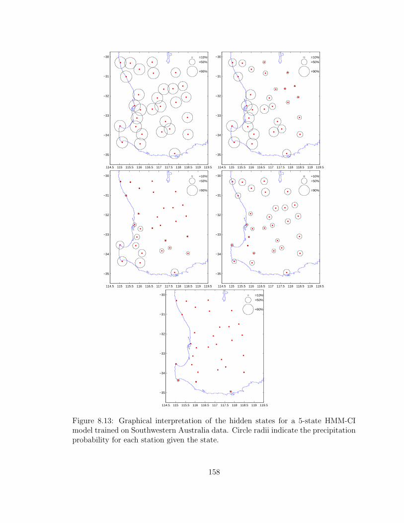
114.5 115 115.5 116 116.5 117 117.5 118 118.5 119 119.5

−35

−34

−33

−32

−31

−30

=90%

=50%

=10%

114.5 115 115.5 116 116.5 117 117.5 118 118.5 119 119.5

−35

−34

−33

−32

−31

−30

=90%

=50%

=10%

114.5 115 115.5 116 116.5 117 117.5 118 118.5 119 119.5

−35

−34

−33

−32

−31

−30

=90%

=50%

=10%

114.5 115 115.5 116 116.5 117 117.5 118 118.5 119 119.5

−35

−34

−33

−32

−31

−30

=90%

=50%

=10%

114.5 115 115.5 116 116.5 117 117.5 118 118.5 119 119.5

−35

−34

−33

−32

−31

−30

=90%

=50%

=10%

Figure 8.13: Graphical interpretation of the hidden states for a 5-state HMM-CImodel trained on Southwestern Australia data. Circle radii indicate the precipitationprobability for each station given the state.

158

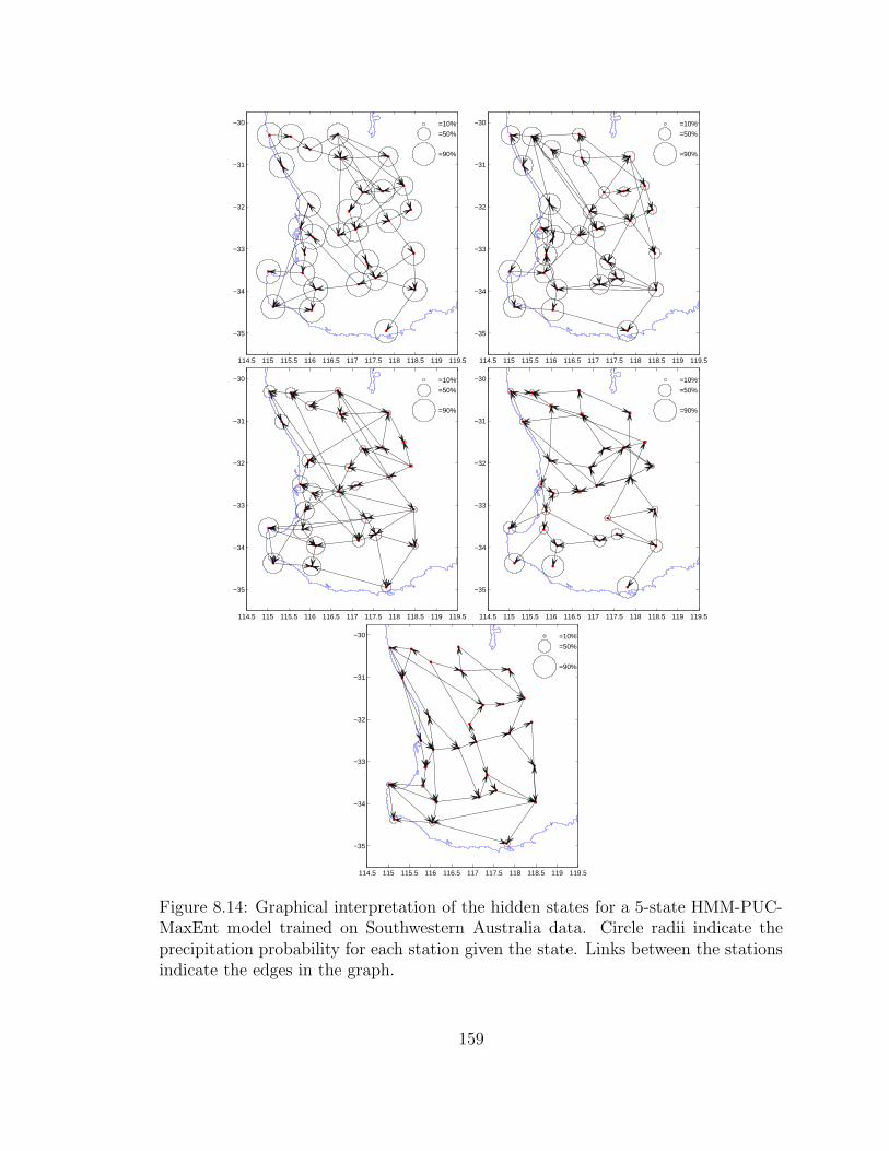
114.5 115 115.5 116 116.5 117 117.5 118 118.5 119 119.5

−35

−34

−33

−32

−31

−30

=90%

=50%

=10%

114.5 115 115.5 116 116.5 117 117.5 118 118.5 119 119.5

−35

−34

−33

−32

−31

−30

=90%

=50%

=10%

114.5 115 115.5 116 116.5 117 117.5 118 118.5 119 119.5

−35

−34

−33

−32

−31

−30

=90%

=50%

=10%

114.5 115 115.5 116 116.5 117 117.5 118 118.5 119 119.5

−35

−34

−33

−32

−31

−30

=90%

=50%

=10%

114.5 115 115.5 116 116.5 117 117.5 118 118.5 119 119.5

−35

−34

−33

−32

−31

−30

=90%

=50%

=10%

Figure 8.14: Graphical interpretation of the hidden states for a 5-state HMM-PUC-MaxEnt model trained on Southwestern Australia data. Circle radii indicate theprecipitation probability for each station given the state. Links between the stationsindicate the edges in the graph.

159

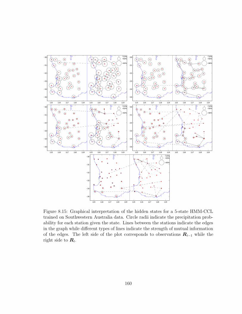
115 116 117 118 119 115 116 117 118 119

−35

−34

−33

−32

−31

−30

=90%

=50% =10%

115 116 117 118 119 115 116 117 118 119

−35

−34

−33

−32

−31

−30

=90%

=50% =10%

115 116 117 118 119 115 116 117 118 119

−35

−34

−33

−32

−31

−30

=90%

=50% =10%

115 116 117 118 119 115 116 117 118 119

−35

−34

−33

−32

−31

−30

=90%

=50% =10%

115 116 117 118 119 115 116 117 118 119

−35

−34

−33

−32

−31

−30

=90%

=50% =10%

Figure 8.15: Graphical interpretation of the hidden states for a 5-state HMM-CCLtrained on Southwestern Australia data. Circle radii indicate the precipitation prob-ability for each station given the state. Lines between the stations indicate the edgesin the graph while different types of lines indicate the strength of mutual informationof the edges. The left side of the plot corresponds to observations Rt−1 while theright side to Rt.

160

−124 −122 −120 −118 −116 −114 −112 −110 −108 −10632

34

36

38

40

42

44

46

48

=90%

=50%

=10%

Figure 8.16: Stations in the Western U.S. region. Circle radii indicate marginalprobabilities of rainfall (> 0mm) at each location.

8.3.3 Western United States

The Western U.S. data was collected from 8 sparsely located stations over 39 90-

day winter seasons (December–February, 1951–1990). Figure 8.16 shows the network

of stations.

The analysis is performed similarly to that of the Southwestern Australia data.

As before, we use leave-one-out cross-validation and the same two different criteria:

the scaled log-likelihood and the average classification error for seasons not in the

training data. Since the stations are sparsely located, we do not expect strong spatial

dependencies; thus, models with additional temporal links are expected to perform

better than the models without them. In addition to the models considered in Sec-

tion 8.3.2 (HMM-CI, HMM-Chains, HMM-CL, HMM-CCL, HMM-PUC-MaxEnt,

and AR-HMM-PUC-MaxEnt), we consider several stateless models with temporal

161

dependencies. These are degenerative cases (K = 1) of the HMM-Chains, HMM-

CCL, and AR-HMM-PUC-MaxEnt; these models are essentially dynamic Bayesian

networks (DBNs) with transitions defined as CI, conditional Chow-Liu forest, and

PUC-MaxEnt distributions, respectively. We will denote these models as DBN

Chains, DBN CCL, and DBN AR-PUC-MaxEnt.9 The comparison plot of scaled log-

likelihood for these models across different K is shown in Figure 8.17. In contrast to

Southwestern Australia data, HMMs with additional temporal links significantly out-

perform HMMs without them. It is also worth noting that AR-HMM-PUC-MaxEnt

achieves high out-of-sample log-likelihood even for small (K = 2, 3) number of hidden

states.

The scatter plots in Figure 8.18 show the scaled log-likelihoods and classification

errors for the models on the left-out sets. K is chosen subjectively according to the

scaled log-likelihood for each model as we want to select a model providing a good

fit with the smallest number of hidden states. The y-axis is the performance of the

AR-HMM-PUC-MaxEnt model, and the x-axis represents the performance of the

other HMMs (shown with different symbols). Higher implies better performance for

log-likelihood (on the left) and worse for error (on the right). The number of hidden

states for the models is chosen to correspond to high average values of out-of-sample

log-likelihood and so that the number of free parameters for different types of models

is about the same. These plots lead us to the same conclusion as Figure 8.17, that

models with temporal links fit this data better as all three models with explicitly

model temporal dependencies outperform the two models without them.

9DBN Chains is just a model with independent Markov chains. Kirshner et al. (2004) used DBNCCL under the name of chain Chow-Liu forests (CCLF).

162

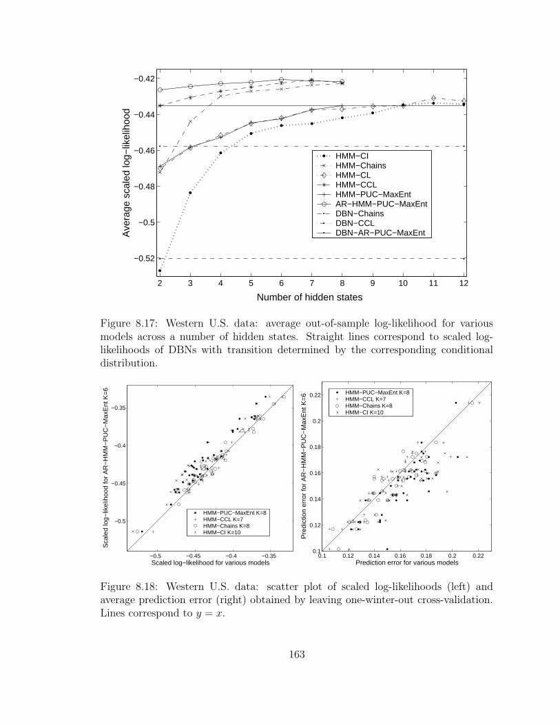
2 3 4 5 6 7 8 9 10 11 12

−0.52

−0.5

−0.48

−0.46

−0.44

−0.42


Ave

rage

sca

led

log−

likel

ihoo

d

HMM−CIHMM−ChainsHMM−CLHMM−CCLHMM−PUC−MaxEntAR−HMM−PUC−MaxEntDBN−ChainsDBN−CCLDBN−AR−PUC−MaxEnt

Figure 8.17: Western U.S. data: average out-of-sample log-likelihood for variousmodels across a number of hidden states. Straight lines correspond to scaled log-likelihoods of DBNs with transition determined by the corresponding conditionaldistribution.

−0.5 −0.45 −0.4 −0.35

−0.5

−0.45

−0.4

−0.35

Scaled log−likelihood for various models

Sca

led

log−

likel

ihoo

d fo

r A

R−

HM

M−

PU

C−

Max

Ent

K=

6

HMM−PUC−MaxEnt K=8HMM−CCL K=7HMM−Chains K=8HMM−CI K=10

0.1 0.12 0.14 0.16 0.18 0.2 0.220.1

0.12

0.14

0.16

0.18

0.2

0.22

Prediction error for various models

Pre

dict

ion

erro

r fo

r A

R−

HM

M−

PU

C−

Max

Ent

K=

6 HMM−PUC−MaxEnt K=8HMM−CCL K=7HMM−Chains K=8HMM−CI K=10

Figure 8.18: Western U.S. data: scatter plot of scaled log-likelihoods (left) andaverage prediction error (right) obtained by leaving one-winter-out cross-validation.Lines correspond to y = x.

163

Examples of the conditional Chow-Liu forest structures learned by the model are

shown in Figure 8.19 for the 7-state HMM-CCL model trained on all 39 years of data.

The states learned by the model correspond to a variety of wet and dry spatial and

temporal patterns. Corresponding plots of the AR-HMM-PUC-MaxEnt with K = 6

are shown in Figure 8.20. The weather states match up remarkably well except for

the third row states of the HMM-CCL being merged into one (third row left) state

of the 6-state AR-HMM-PUC-MaxEnt. Both models generate data with statistics

very similar to the historical data, matching the precipitation probabilities exactly

(Figure 8.22 left), while closely matching both persistence (Figure 8.22 right) and

correlation (Figure 8.21).

164

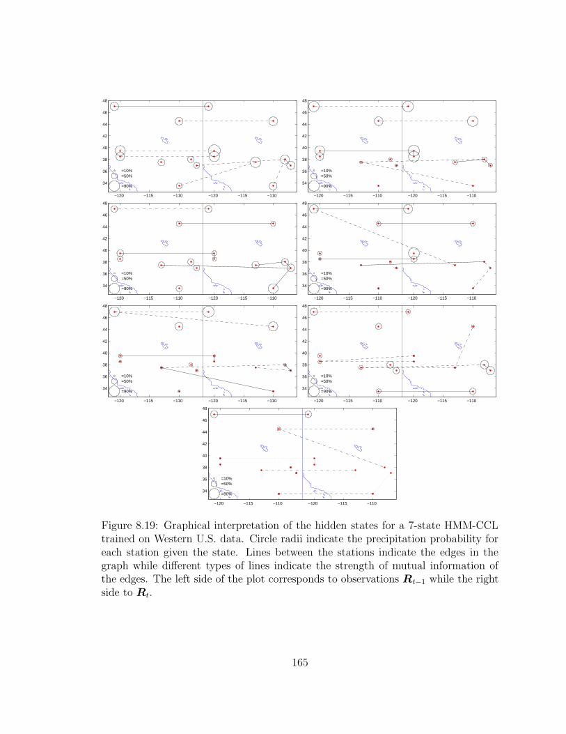
−120 −115 −110 −120 −115 −110

34

36

38

40

42

44

46

48

=90%

=50% =10%

−120 −115 −110 −120 −115 −110

34

36

38

40

42

44

46

48

=90%

=50% =10%

−120 −115 −110 −120 −115 −110

34

36

38

40

42

44

46

48

=90%

=50% =10%

−120 −115 −110 −120 −115 −110

34

36

38

40

42

44

46

48

=90%

=50% =10%

−120 −115 −110 −120 −115 −110

34

36

38

40

42

44

46

48

=90%

=50% =10%

−120 −115 −110 −120 −115 −110

34

36

38

40

42

44

46

48

=90%

=50% =10%

−120 −115 −110 −120 −115 −110

34

36

38

40

42

44

46

48

=90%

=50% =10%

Figure 8.19: Graphical interpretation of the hidden states for a 7-state HMM-CCLtrained on Western U.S. data. Circle radii indicate the precipitation probability foreach station given the state. Lines between the stations indicate the edges in thegraph while different types of lines indicate the strength of mutual information ofthe edges. The left side of the plot corresponds to observations Rt−1 while the rightside to Rt.

165

−120 −115 −110 −120 −115 −110

34

36

38

40

42

44

46

48

=90%

=50% =10%

−120 −115 −110 −120 −115 −110

34

36

38

40

42

44

46

48

=90%

=50% =10%

−120 −115 −110 −120 −115 −110

34

36

38

40

42

44

46

48

=90%

=50% =10%

−120 −115 −110 −120 −115 −110

34

36

38

40

42

44

46

48

=90%

=50% =10%

−120 −115 −110 −120 −115 −110

34

36

38

40

42

44

46

48

=90%

=50% =10%

−120 −115 −110 −120 −115 −110

34

36

38

40

42

44

46

48

=90%

=50% =10%

Figure 8.20: Graphical interpretation of the hidden states for a 6-state AR-HMM-PUC-MaxEnt trained on Western U.S. data. Circle radii indicate the precipitationprobability for each station given the state. Edges between the stations indicate theedges in the graph. The left side of the plot corresponds to observations Rt−1 whilethe right side to Rt.

166

0 0.5 1 0 0.02 0.04 0.06 0.08 0 0.02 0.04 0.06 0.08

Figure 8.21: Western U.S. data: correlation matrix of rainfall daily occurrence (left),absolute difference between the correlation matrix of the data and the correlation ofthe data simulated from a 6-state AR-HMM-PUC-MaxEnt (middle) and a 7-stateHMM-CCL (right). The average absolute difference for non-diagonal entries is 0.019for AR-HMM-PUC-MaxEnt and 0.013 for HMM-CCL.

0.2 0.3 0.4 0.5 0.6 0.70.2

0.3

0.4

0.5

0.6

0.7


Sim

ulat

ed p

reci

pita

tion

prob

abili

ties

AR−HMM−PUC−MaxEnt K=6HMM−CCL K=7

0.5 0.55 0.6 0.65 0.7 0.75 0.8 0.85

0.5

0.55

0.6

0.65

0.7

0.75

0.8

0.85

Actual persistence

Sim

ulat

ed p

ersi

sten

ce

AR−HMM−PUC−MaxEnt K=6HMM−CCL K=7

Figure 8.22: Western U.S. data: scatter plot of the precipitation probabilities (left)and the persistence (right) for each station of the actual data versus the simulateddata from various models. Straight lines correspond to y = x.

167

139 140 141 142 143 144 145 146 147 148 149 150−23

−22

−21

−20

−19

−18

−17

−16

−15

0.1

0.3

0.5

0.7

0.9

Figure 8.23: Stations in the Queensland (Northeastern Australia) region. Circle radiiindicate marginal probabilities of rainfall (≥ 1mm) at each location.

8.3.4 Queensland (Northeastern Australia)

This data was collected from 11 stations over 40 197-day austral summer periods

(October 1–April, 1958–1998). This data set is derived from the Patched Point

Dataset (PPD) (Jeffrey et al., 2001). Figure 8.23 shows the network of stations.

Judging just by the locations of the stations, the data set should be fit best by

models allowing for both temporal and spatial dependencies (HMM-CCL and AR-

HMM-PUC-MaxEnt) as the stations are sparsely located except for the cluster in

the north.

For this set, we use leave-eight-out (five-fold) cross-validation to evaluate the mod-

els. In addition to the scaled log-likelihood, we would also consider out-of-sample

168

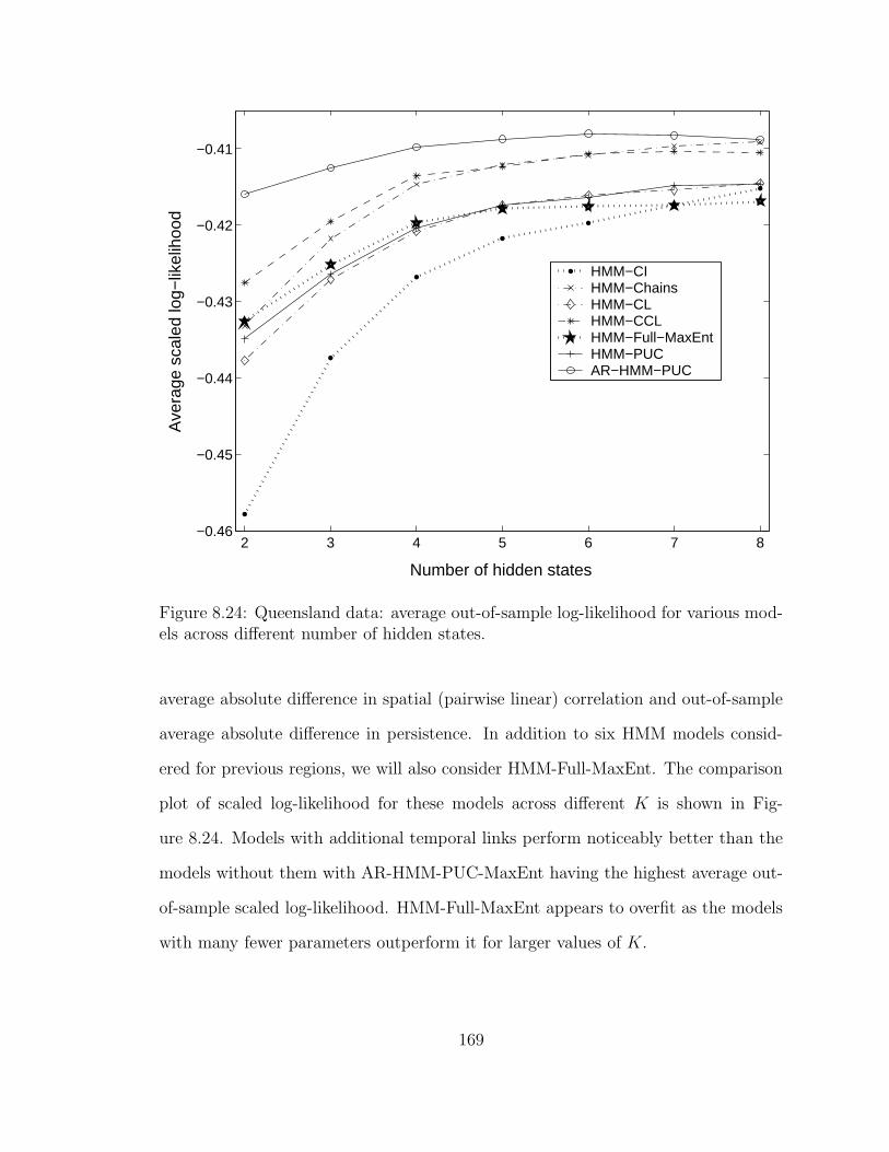
2 3 4 5 6 7 8−0.46

−0.45

−0.44

−0.43

−0.42

−0.41


Ave

rage

sca

led

log−

likel

ihoo

d

HMM−CIHMM−ChainsHMM−CLHMM−CCLHMM−Full−MaxEntHMM−PUCAR−HMM−PUC

Figure 8.24: Queensland data: average out-of-sample log-likelihood for various mod-els across different number of hidden states.

average absolute difference in spatial (pairwise linear) correlation and out-of-sample

average absolute difference in persistence. In addition to six HMM models consid-

ered for previous regions, we will also consider HMM-Full-MaxEnt. The comparison

plot of scaled log-likelihood for these models across different K is shown in Fig-

ure 8.24. Models with additional temporal links perform noticeably better than the

models without them with AR-HMM-PUC-MaxEnt having the highest average out-

of-sample scaled log-likelihood. HMM-Full-MaxEnt appears to overfit as the models

with many fewer parameters outperform it for larger values of K.

169

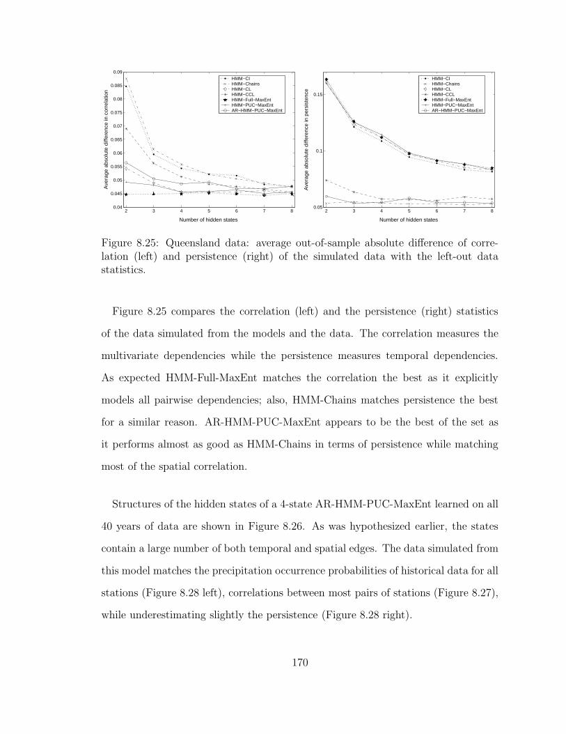
2 3 4 5 6 7 80.04

0.045

0.05

0.055

0.06

0.065

0.07

0.075

0.08

0.085

0.09


Ave

rage

abs

olut

e di

ffere

nce

in c

orre

latio

n

HMM−CIHMM−ChainsHMM−CLHMM−CCLHMM−Full−MaxEntHMM−PUC−MaxEntAR−HMM−PUC−MaxEnt

2 3 4 5 6 7 80.05

0.1

0.15


Ave

rage

abs

olut

e di

ffere

nce

in p

ersi

sten

ce

HMM−CIHMM−ChainsHMM−CLHMM−CCLHMM−Full−MaxEntHMM−PUC−MaxEntAR−HMM−PUC−MaxEnt

Figure 8.25: Queensland data: average out-of-sample absolute difference of corre-lation (left) and persistence (right) of the simulated data with the left-out datastatistics.

Figure 8.25 compares the correlation (left) and the persistence (right) statistics

of the data simulated from the models and the data. The correlation measures the

multivariate dependencies while the persistence measures temporal dependencies.

As expected HMM-Full-MaxEnt matches the correlation the best as it explicitly

models all pairwise dependencies; also, HMM-Chains matches persistence the best

for a similar reason. AR-HMM-PUC-MaxEnt appears to be the best of the set as

it performs almost as good as HMM-Chains in terms of persistence while matching

most of the spatial correlation.

Structures of the hidden states of a 4-state AR-HMM-PUC-MaxEnt learned on all

40 years of data are shown in Figure 8.26. As was hypothesized earlier, the states

contain a large number of both temporal and spatial edges. The data simulated from

this model matches the precipitation occurrence probabilities of historical data for all

stations (Figure 8.28 left), correlations between most pairs of stations (Figure 8.27),

while underestimating slightly the persistence (Figure 8.28 right).

170

140 142 144 146 148 140 142 144 146 148−23

−22

−21

−20

−19

−18

−17

−16

−150.1

0.3

0.5

0.7

0.9

140 142 144 146 148 140 142 144 146 148−23

−22

−21

−20

−19

−18

−17

−16

−150.1

0.3

0.5

0.7

0.9

140 142 144 146 148 140 142 144 146 148−23

−22

−21

−20

−19

−18

−17

−16

−150.1

0.3

0.5

0.7

0.9

140 142 144 146 148 140 142 144 146 148−23

−22

−21

−20

−19

−18

−17

−16

−150.1

0.3

0.5

0.7

0.9

Figure 8.26: Graphical interpretation of the hidden states for a 4-state AR-HMM-PUC-MaxEnt trained on Queensland data. Circle radii indicate the precipitationprobability for each station given the state. Edges between the stations indicate theedges in the graph. The left side of the plot corresponds to observations Rt−1 whilethe right side to Rt.

171

0 0.2 0.4 0.6 0.8 1 0 0.02 0.04 0.06

Figure 8.27: Queensland data: correlation matrix of rainfall daily occurrence (left),absolute difference between the correlation matrix of the data and the correlationof the data simulated from a 4-state AR-HMM-PUC-MaxEnt (right). The averageabsolute difference for non-diagonal entries is 0.013.

0.1 0.15 0.2 0.25 0.3 0.35 0.4 0.450.1

0.15

0.2

0.25

0.3

0.35

0.4

0.45


Sim

ulat

ed p

reci

pita

tion

prob

abili

ties

AR−HMM−PUC−MaxEnt K=4

0.35 0.4 0.45 0.5 0.55 0.6 0.65 0.70.35

0.4

0.45

0.5

0.55

0.6

0.65

Actual persistence

Sim

ulat

ed p

ersi

sten

ce

AR−HMM−PUC−MaxEnt K=4

Figure 8.28: Queensland data: scatter plot of the precipitation probabilities (left)and the persistence (right) for each station of the actual data versus the simulateddata from various models. Straight lines correspond to y = x.

172

8.4 Summary

We applied the models from Chapter 6 to four daily precipitation occurrence data

sets of various strengths of multivariate and temporal dependencies. For each set,

the best model depends on whether spatial or temporal dependence is stronger.

However, the models that learn both temporal and multivariate links perform well

in all cases; from these models, AR-HMM-PUC-MaxEnt fits the data a little better

at the expense of larger number of parameters. However, AR-HMM-PUC-MaxEnt

can be used with smaller number of hidden states cutting the number of parameters

while reducing the fit only marginally.

Novel models allowing to learn multivariate and temporal links (e.g., HMM-CCL,

AR-HMM-PUC-MaxEnt) show a lot of promise for modeling multivariate vector time

series. We believe that their advantages over simpler models would be even more

evident on data sets with vectors of higher dimensionality as these models can extract

the structure corresponding to the strongest dependencies in the data.

173

Chapter 9

Summary and Future Directions

In this thesis we introduced a number of new models and corresponding training

algorithms for modeling multivariate time series or just multivariate data. The ma-

jority of the results address categorical data although some of the models can be

extended, sometimes trivially, to real-valued domains. We have empirically shown

that given sufficient data, the models can correctly estimate the parameters. Finally,

we applied the models to the domain of multi-site precipitation occurrence modeling

and obtained superior predictive accuracy compared to similar models and better

modeled persistence and spatial correlation. In this concluding chapter of the thesis,

we summarize the main contributions and outline future directions and challenges.

9.1 List of Contributions

1. Introduced Chow-Liu trees for use with HMMs and developed a cor-

responding parameter estimation algorithm. The use of Chow-Liu trees

in conjunction with hidden Markov models allows efficient preservation of some

of the multivariate dependencies in the multivariate time series data. Due to

174

the efficiency of the Chow-Liu tree algorithm, the Chow-Liu model can be used

as a probability distribution within each hidden state with only a reasonable

increase in computational complexity. The amount of data need to train the

model is not overly large as only pairwise variable interactions are considered

in each hidden state.

2. Extended Chow-Liu trees to the conditional distribution case and

developed a corresponding AR-HMM together with their parameter

estimation algorithms. The conditional Chow-Liu (CCL) forests allow us to

learn the tree-structure of the conditional distribution with Chow-Liu trees on

the joint distributions as its special case. In most cases, the asymptotic compu-

tational complexity of the conditional Chow-Liu model is the same as that of

the original Chow-Liu model, so the extended model is very efficient. This com-

putational efficiency allows the use of CCL forests with AR-HMMs; the main

advantage is that the new hybrid HMM-CCL model can select automatically

the strongest dependencies from both temporal and multivariate dependencies

thus improving the quality of the model. As with HMMs with Chow-Liu trees,

the combined model can often accurately estimate the parameters with only a

limited amount of data available.

3. Introduced a model allowing joint and conditional distributions with

structures less restrictive than trees; proposed a structure-learning

algorithm for the model. The product of univariate conditional exponen-

tials (PUC-MaxEnt) model allows us to learn a distribution with an arbitrary

Bayesian network on categorical valued data. This model can be thought of as

a generalization of CCL forests although the structure learning and parameter

estimation for this model can be significantly more involved than that in the

175

CCL forests case. One of the most attractive features of this model (as com-

pared to other multivariate exponential models) is the clarity of the parameter

estimation and the ease of its implementation. Since the model is represented as

a product of univariate conditional distributions, the parameter estimation can

be broken down into independent updates of univariate conditional exponential

distributions for each variable and can likely be parallelized. This model also

avoids summing over large number of variables in the parameter estimation.

To estimate the structure of the model, we proposed a greedy algorithm that

uses an approximation to the log-likelihood improvement achieved by adding

each candidate edge.

4. Incorporated PUC-MaxEnt with HMMs. The new model can be used to

model time series with dense multivariate or temporal dependence structures.

This model, however, requires a substantial amount of data and is computa-

tionally quite involved.

5. Analyzed the Gaussian counterpart of the Chow-Liu tree model.

Since pairwise variable dependencies in multivariate normal distributions are

encoded in its covariance matrix, we studied the structure of this matrix for

tree-structured multivariate Gaussian distributions. We have derived a closed

form expression for the covariance matrix, detailed the computational complex-

ities of the operations for this tree-structured matrix, outlining several possible

advantages of this model over the saturated model. Finally, we incorporated

this new model into an HMM for modeling of multivariate real-valued time

series.

6. Introduced a new model for efficient modeling of multi-site precip-

itation amounts. This HMM-CI based model allows us to model multi-site

176

precipitation amounts without learning a categorical data model first. Initial

experimental results suggest that the model produces realistic precipitation

simulation (Robertson et al., in preparation).

7. Applied the model to several historical precipitation occurrence data

sets. The study compared how well the models fit the data based on log-

likelihood and spatial and temporal statistics of the data. The data sets varied

in the amount of data, and strengths of bivariate temporal and spatial depen-

dencies.

8. Conducted an empirical simulation study of how well some of the

described models can estimate the true parameters. The experiments

tested how well can a model recover the parameters given various amounts

of simulated data. The experiment was repeated for models with different

entropies.

9. Developed a software suite for parameter estimation and analysis for

the models in the thesis. I developed Unix-based C++ software for data

modeling using HMMs with multivariate distributions in hidden states. The

software is publicly available, and most of the routines and features are being

used by our scientific collaborators, e.g., at IRI and CSIRO.

9.2 Future Directions

1. Models for multivariate real-valued non-Gaussian time series. The

vast majority of the models described in this thesis deal with multivariate cat-

egorical data. However, a large portion of the real-world data does not fit

this criterion; precipitation data is by nature non-negative real-valued (non-

177

Gaussian as a result) and is modeled as binary data because very few reliable

real-valued models are available. The desired models should preserve univari-

ate marginals of the data while capturing multivariate dependencies. Our at-

tempts to incorporate tree-based models for precipitation amounts were fruit-

less as modeling bivariate exponentials (components of marginals) turned out

to be difficult. One possible future direction is the use of copulas (Joe, 1997;

Nelsen, 1998), multivariate cumulative density functions preserving univariate

marginals. These functions may have the desired characteristics to be used

with HMMs in modeling multivariate non-Gaussian real-valued time series.

2. Feature selection for inputs to be used with non-homogeneous

HMMs. The NHMMs described in Section 3.1.2 require input variables. The

sets of potential input variables can be very large. For example, in precipitation

modeling the input sets are usually the variables simulated from a GCM. These

variables are usually computed on a grid at regular time intervals, so there may

be thousands if not millions of potential variables. Since only a small number

of them are potentially useful (and non-relevant variables can degrade the per-

formance), the importance of selecting the right set of variables is significant.

Variable selection from a large set of candidate input variables in a NHMM is

an open problem.

3. Handling missing data. Most of the real-world data has missing values.

For example, precipitation records have gaps, especially the ones from less

developed regions. One option is just to throw the sequences with missing data

away, but in the presence of only a moderate amount of complete data, this

method may impact the accuracy of the models. More desirable is to change

the learning algorithm to allow for missing data. For example, HMM-CI can be

178

modified in a straightforward manner to allow missing observations. Methods

for incorporating missing observations with other models discussed in this thesis

need to be developed. One possibility is to use a Bayesian approach and to

infer distributions over the missing data in the Bayesian framework.

4. Bayesian framework for HMMs for multivariate time series. There

are advantages to using a Bayesian framework for modeling multivariate time

series. One of the reasons, Bayesian framework allows us to incorporate expert

knowledge into the parameter estimation and model selection. For example, for

multi-site precipitation application, we may use geographical and topographical

information in model selection and estimation, e.g., a spatial prior on which

edges could be included in the model.

179

Bibliography

D. J. Allcroft and C. A. Glasbey. A latent Gaussian Markov random-field model

for spatiotemporal rainfall disaggregation. Journal of the Royal Statistical Society

Series C (Applied Statistics), 52(4):487–498, 2003.

S. Arngborg, D. G. Corneil, and A. Proskurowski. The complexity of finding embed-

dings in a k-tree. SIAM Journal on Algebraic and Discrete Methods, 8(2):277–284,

April 1987.

J. R. Ashford and R. R. Sowden. Multi-variate probit analysis. Biometrics, 26(3):

535–546, 1970.

F. R. Bach and M. I. Jordan. Thin junction trees. In T. G. Dietterich, S. Becker,

and Z. Ghahramani, editors, Advances in Neural Information Processing Systems

14, pages 569–576, Cambridge, MA, 2002. MIT Press.

P. Baldi and S. Brunak. Bioinformatics. MIT Press, 2nd edition, 2001.

A. Bardossy and E. J. Plate. Space-time model for daily rainfall using atmospheric

circulation patterns. Water Resources Research, 28:1247–1259, 1992.

L. E. Baum and T. Petrie. Statistical inference for probabilistic functions of finite

state Markov chains. Annals of Mathematical Statistics, 37(6):1554–1563, 1966.

180

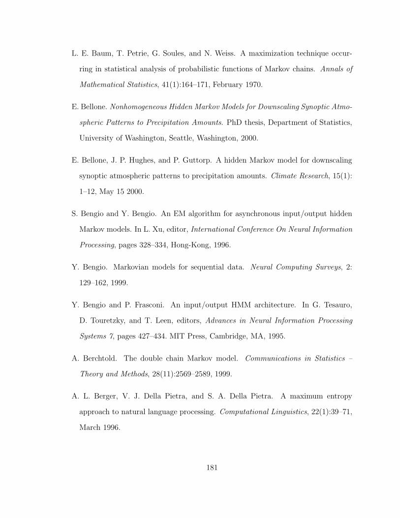
L. E. Baum, T. Petrie, G. Soules, and N. Weiss. A maximization technique occur-

ring in statistical analysis of probabilistic functions of Markov chains. Annals of

Mathematical Statistics, 41(1):164–171, February 1970.

E. Bellone. Nonhomogeneous Hidden Markov Models for Downscaling Synoptic Atmo-

spheric Patterns to Precipitation Amounts. PhD thesis, Department of Statistics,

University of Washington, Seattle, Washington, 2000.

E. Bellone, J. P. Hughes, and P. Guttorp. A hidden Markov model for downscaling

synoptic atmospheric patterns to precipitation amounts. Climate Research, 15(1):

1–12, May 15 2000.

S. Bengio and Y. Bengio. An EM algorithm for asynchronous input/output hidden

Markov models. In L. Xu, editor, International Conference On Neural Information

Processing, pages 328–334, Hong-Kong, 1996.

Y. Bengio. Markovian models for sequential data. Neural Computing Surveys, 2:

129–162, 1999.

Y. Bengio and P. Frasconi. An input/output HMM architecture. In G. Tesauro,

D. Touretzky, and T. Leen, editors, Advances in Neural Information Processing

Systems 7, pages 427–434. MIT Press, Cambridge, MA, 1995.

A. Berchtold. The double chain Markov model. Communications in Statistics –

Theory and Methods, 28(11):2569–2589, 1999.

A. L. Berger, V. J. Della Pietra, and S. A. Della Pietra. A maximum entropy

approach to natural language processing. Computational Linguistics, 22(1):39–71,

March 1996.

181

R. Bhar and S. Hamori. Hidden Markov Models: Applications to Financial Eco-

nomics. Advanced Studies in Theoretical and Applied Econometrics. Kluwer, 2004.

J. Bilmes. Dynamic Bayesian multinets. In Proceedings of the 16th Annual Conference

on Uncertainty in Artificial Intelligence (UAI-00), pages 38–45, San Francisco, CA,

2000. Morgan Kaufmann Publishers.

J. Bilmes, 2004. Personal communications.

J. A. Bilmes. Burried Markov models for speech recognition. In IEEE International

Conference on Acoustics, Speech, and Signal Processing (ICASSP ’99), volume 2,

pages 713–716, 1999.

M. Brand, N. Oliver, and A. Pentland. Coupled hidden Markov models for complex

action recognition. In Proceedings of IEEE Conference on Computer Vision and

Pattern Recognition, pages 994–999, 1997.

P. J. Brockwell and R. A. Davis. Introduction to Time Series and Forecasting.

Springer Texts in Statistics. Springer, second edition, 2002.

D. Brown. A note on approximations to discrete probability distributions. Informa-

tion and Control, 2:386–392, 1959.

S. Chib. Calculating posterior distributions and modal estimates in Markov mixture

models. Journal of Econometrics, 75(1):79–97, November 1996.

S. Chib and E. Greenberg. Analysis of multivariate probit models. Biometrika, 85

(2):347–361, June 1998.

D. Chickering, D. Heckerman, and C. Meek. A Bayesian approach to learning

Bayesian networks with local structure. In Proceedings of Thirteenth Conference

182

on Uncertainty in Artificial Intelligence, pages 80–89. Morgan Kaufmann, August

1997.

D. M. Chickering. Learning Bayesian networks is NP-complete. In D. Fisher and H.-J.

Lenz, editors, Learning from data: AI and statistics V, pages 121–130. Springer-

Verlag, New York, 1996.

C. K. Chow and C. N. Liu. Approximating discrete probability distributions with

dependence trees. IEEE Transactions on Information Theory, IT-14(3):462–467,

May 1968.

A. S. Cofino, R. Cano, C. Sordo, and J. M. Gutierrez. Bayesian networks for prob-

abilistic weather prediction. In Proceedings of the 15th Eureopean Conference on

Artificial Intelligence, ECAI’2002, pages 695–699, 2002.

T. H. Cormen, C. E. Leiserson, and R. L. Rivest. Introduction to Algorithms. The

MIT Electrical Engineering and Computer Science Series. MIT Press/McGraw

Hill, 1990.

T. M. Cover and J. A. Thomas. Elements of Information Theory. Wiley, New York,

1991.

R. G. Cowell, A. P. Dawid, S. L. Lauritzen, and D. J. Spiegelhalter. Probabilistic

Networks and Expert Systems. Statistics for Engineering and Information Science.

Springer-Verlag, New York, 1st edition, 1999.

D. Cox and N. Wermuth. Multivariate Dependencies – Models, analysis and interpre-

tation, volume 67 of Monographs on Statistics and Applies Probability. Chapman

& Hall, 1996.

183

D. R. Cox and V. Isham. A simple spatial-temporal model of rainfall. Proceedings of

the Royal Society of London Series A – Mathematical, Physical, and Engineering

Sciences, 415(1849):317–328, February 1988.

I. Csiszar. I-divergence geometry of probability distributions and minimization prob-

lems. Annals of Probability, 3(1):146–158, 1975.

J. N. Darroch and D. Ratcliff. Generalized iterative scaling for log-linear models.

The Annals of Mathematical Statistics, 43(5):1470–1480, October 1972.

S. Della Pietra, V. Della Pietra, and J. Lafferty. Inducing features of random fields.

IEEE Transactions on Pattern Analysis and Machine Intelligence, 19(4):380–393,

April 1997.

A. P. Dempster, N. M. Laird, and D. B. Rubin. Maximum likelihood from in-

complete data via EM algorithm. Journal of the Royal Statistical Society Series

B-Methodological, 39(1):1–38, 1977.

M. N. Do. Fast approximation of Kullback-Leibler distance for dependence trees

and hidden Markov models. IEEE Signal Processing Letters, 10(4):115–118, April

2003.

R. O. Duda, P. E. Hart, and D. G. Stork. Pattern Classification. John Wiley & Sons,

New York, second edition, 2000.

N. Friedman. Learning belief networks in the presence of missing values and hidden

variables. In Proceedings of the Fourteenth International Conference on Machine

Learning (ICML-97), 1997.

N. Friedman and M. Goldszmidt. Learning Bayesian networks with local structure.

In E. Horvitz and F. V. Jensen, editors, Proceedings of the Twelfth Conference on

184

Uncertainty in Artificial Intelligence, pages 252–262. Morgan Kaufmann, August

1996.

D. Geiger and D. Heckerman. Knowledge representation and inference in similarity

networks and Bayesian multinets. Artificial Intelligence, 82(1-2):45–74, April 1996.

A. Genz. Comparison of methods for the computation of multivariate normal prob-

abilities. Computing Science and Statistics, 25:400–405, 1993.

A. Genz. Numerical computation of rectangular bivariate and trivariate normal and

t probabilities. Statistics and Computing, 14:151–160, 2004.

Z. Ghahramani. An introduction to hidden Markov models and Bayesian networks.

International Journal of Pattern Recognition and Artificial Intelligence, 15(1):9–

42, February 2001.

C. R. Goodall and M. J. Phelan. Edge-preserving smoothing and the assessment of

point process models for Gate rainfall fields. In Statistical Inference in Stochastic

Processes, pages 35–66. Marce Dekker, Inc., 1991.

J. Goodman. Sequential conditional generalized iterative scaling. In Proceedings of

the 40th Annual Meeting of the Association for Computational Linguistics (ACL),

pages 9–16, July 2002.

J. Grim. On structural approximating multivariate discrete probability-distributions.

Kybernetika, 20(1):1–17, 1984.

P. Guttorp. Stochastic Modeling of Scientific Data. Chapman & Hall, 1995.

J. D. Hamilton. Time Series Analysis. Princeton University Press, Princeton, New

Jersey, 1994.

185

J. M. Hammersley and P. E. Clifford. Markov fields on finite graphs and lattices.

Unpublished manuscript, 1971.

L. E. Hay, G. McCabe, D. M. Wolock, and M. A. Ayers. Simulation of precipitation

by weather type analysis. Water Resources Research, 27:493–501, 1991.

J. P. Hughes and P. Guttorp. Incorporating spatial dependence and atmospheric

data in a model of precipitation. Journal of Applied Meteorology, 33(12):1503–

1515, December 1994.

J. P. Hughes, P. Guttorp, and S. P. Charles. A non-homogeneous hidden Markov

model for precipitation occurrence. Journal of the Royal Statistical Society Series

C Applied Statistics, 48(1):15–30, 1999.

S. J. Jeffrey, J. O. Carter, K. B. Moodie, and A. R. Beswick. Using spatial interpo-

lation to construct a comprehensive archive of Australian climate data. Environ-

mental Modelling & Software, 16(4):309–330, 2001.

F. Jelinek. Statistical Methods for Speech Recognition. The MIT Press, 1998.

F. V. Jensen and F. Jensen. Optimal junction trees. In Proceedings of the Tenth

Conference on Uncertainty in Artificial Intelligence, pages 360–366, 1994.

R. Jirousek and S. Preucil. On the effective implementation of the iterative propor-

tional fitting procedure. Computational Statistics & Data Analysis, 19:177–189,

1995.

H. Joe. Multivariate Models and Dependence Concepts, volume 73 of Monographs on

Statistics and Applied Probability. Chapman & Hall/CRC, 1997.

M. I. Jordan and R. A. Jacobs. Hierarchical mixtures of experts and the EM algo-

rithm. Neural Computation, 6:181–214, 1994.

186

R. W. Katz. Probabilistic models. In Probability, statistics and decision making in

the atmospheric sciences, pages 261–288. Westview Press, Boulder, CO, 1985.

S. Kirshner, S. Parise, and P. Smyth. Unsupervised learning with permuted data.

In T. Fawcett and N. Mishra, editors, Proceedings of the Twentieth International

Conference on Machine Learning (ICML-2003), pages 345–352. AAAI Press, 2003.

S. Kirshner, P. Smyth, and A. W. Robertson. Conditional Chow-Liu tree structures

for modeling discrete-valued vector time series. In M. Chickering and J. Halpern,

editors, Proceedings of the Twentieth Conference on Uncertainty in Artificial In-

telligence (UAI-04), pages 317–324. AUAI Press, 2004.

U. Kjærulff. Triangulation of graphs – algorithms giving small total state space.

Technical report, Aalborg University, 1990.

S. Kotz, N. Balakrishnan, and N. L. Johnson. Continuous Multivariate Distributions,

Volume 1: Models and Applications. Wiley Series in Probability and Statistics.

John Wiley & Sons, second edition, 2000.

A. Krogh, M. Brown, I. S. Mian, K. Sj olander, and D. Haussler. Hidden Markov

models in computational biology – applications to protein modeling. Journal of

Molecular Biology, 235(5):1501–1531, February 1994.

F. R. Kschischang, B. J. Frey, and H.-A. Loeliger. Factor graphs and the sum-product

algorithm. IEEE Transactions on Information Theory, 47(2):498–519, February

2001.

J. Kwon and K. P. Murphy. Modeling freeway traffic using coupled HMMs. Technical

report, UC Berkeley, 2000.

187

J. D. Lafferty, A. McCallum, and F. C. N. Pereira. Conditional random fields:

Probabilistic models for segmenting and labeling sequence data. In C. E. Brodley

and A. P. Danyluk, editors, Proceedings of the Eighteenth International Conference

on Machine Learning (ICML 01), pages 282–289. Morgan Kaufmann, 2001.

S. L. Lauritzen. Graphical Models. Oxford Statistical Science Series. Oxford Univer-

sity Press, 1996.

E. Lesaffre and H. Kaufmann. Existence and uniqueness of the maximum-likelihood

estimator for a multivariate probit model. Journal of the American Statistical

Association, 87(419):805–811, September 1992.

I. L. MacDonald and W. Zucchini. Hidden Markov and Other Models for Discrete-

valued Time Series. Number 70 in Monographs on Statistics and Applied Proba-

bility. Chapman & Hall, 1997.

R. Malouf. A comparison of algorithms for maximum entropy parameter estimation.

In Proceedings of the Sixth Conference on Natural Language Learning, pages 49–55,

2002.

P. McCullagh and J. A. Nelder. Generalized Linear Models, volume 37 of Monographs

on Statistics and Applied Probability. Chapman & Hall/CRC, second edition, 1989.

G. McLachlan and D. Peel. Finite Mixture Models. Wiley Series in Probability and

Statistics. John Wiley & Sons, Inc., 2000.

M. Meila. An accelerated Chow and Liu algorithm: Fitting tree distributions to

high-dimensional sparse data. In I. Bratko and S. Dzeroski, editors, Proceedings

of the Sixteenth International Conference on Machine Learning (ICML’99), pages

249–57. Morgan Kaufmann, 1999.

188

M. Meila and M. I. Jordan. Markov mixture of experts. In R. Murray-Smith and

T. A. Johanssen, editors, Multiple Model Approaches to Nonlinear Modelling and

Control. Taylor and Francis, 1996.

M. Meila and M. I. Jordan. Learning with mixtures of trees. Journal of Machine

Learning Research, 1(1):1–48, October 2000.

T. P. Minka. A Family of Algorithms for Approximate Bayesian Inference. PhD

thesis, Massachusetts Institute of Technology, January 2001.

K. P. Murphy. Dynamic Bayesian Networks: Representation, Inference and Learning.

PhD thesis, University of California, Berkeley, Berkeley, CA, July 2002.

R. B. Nelsen. Introduction to Copulas, volume 139 of Lecture Notes in Statistics.

Springer, 1998.

D. Pavlov, A. Popescul, D. M. Pennock, and L. H. Ungar. Mixtures of conditional

maximum entropy models. In T. Fawcett and N. Mishra, editors, Proceedings of

the Twentieth International Conference on Machine Learning (ICML 2003), pages

584–591. AAAI Press, 2003.

J. Pearl. Probabilistic Reasoning in Intelligent Systems: Networks of Plausible Infer-

ence. Morgan Kaufmann Publishers, Inc., San Francisco, California, 1988.

D. Pelleg and A. Moore. Using Tarjan’s red rule for fast dependency tree construc-

tion. In S. T. S. Becker and K. Obermayer, editors, Advances in Neural Information

Processing Systems 15, pages 801–808. MIT Press, Cambridge, MA, 2003.

A. B. Poritz. Linear predictive hidden Markov models and the speech signal. In

Proceedings of the International Conferences on Acoustics, Speech and Signal Pro-

cessing (ICASSP 82), volume 2, pages 1291–1294. IEEE, 1982.

189

W. H. Press, S. A. Teukolsky, W. V. Vetterling, and B. P. Flannery. Numerical

Recipes in C: The Art of Scientific Computing. Cambridge University Press, 2nd

edition, 1992.

L. R. Rabiner. A tutorial on hidden Markov models and selected applications in

speech recognition. Proceedings of IEEE, 77(2):257–286, February 1989.

B. Rajagopalan and U. Lall. A k-nearest-neighbor simulator for daily precipitation

and other weather variables. Water Resources Research, 35(10):3089–3101, Octo-

ber 1999.

D. A. Randall, editor. General Circulation Model Development: Past, Present, and

Future, volume 70 of International Geophysics Series. Academic Press, 2000.

C. Raphael. Automatic segmentation of acoustic musical signals using hidden Markov

models. IEEE Transactions on Pattern Analysis and Machine Intelligence, 21(4):

360–370, April 1999.

S. Raudys. Statistical and Neural Classifiers: An Integrated Approach to Design.

Advances in Pattern Recognition. Springer, 2001.

A. W. Robertson, S. Kirshner, and P. Smyth. Hidden Markov models for modeling

daily rainfall occurrence over Brazil. Technical Report 03-27, School of Information

and Computer Science, University of California, Irvine, 2003.

A. W. Robertson, S. Kirshner, and P. Smyth. Downscaling of daily rainfall occurrence

over Northeast Brazil using a hidden Markov model. Journal of Climate, 17(22):

4407–4424, November 2004.

A. W. Robertson, S. Kirshner, P. Smyth, B. Bates, and S. Charles. Subseasonal-

190

to-interdecadal variability of the Australian monsoon over north Queensland, in

preparation.

R. Rosenfeld. Adaptive Statistical Language Modeling: A Maximum Entropy Ap-

proach. PhD thesis, Carnegie Mellon University, Pittsburgh, PA, April 1994.

B. Sanso and L. Guenni. Venezuelan rainfall data analysed by using a Bayesian space-

time model. Journal of the Royal Statistical Society Series C (Applied Statistics),

48:345–362, 1999.

S. L. Scott. Bayesian methods for hidden Markov models: Recursive computing in

the 21st century. Journal of the American Statistical Association, 97(457):337–351,

March 2002.

M. A. Semenov and J. R. Porter. Climatic variability and the modeling of crop yields.

Agricultural and Forest Meteorology, 73(3-4):265–283, March 1995.

R. D. Shachter. Bayes-Ball: The rational pastime (for determining irrelevance and

requisite information in belief networks and influence diagrams). In G. F. Cooper

and S. Moral, editors, UAI ’98: Proceedings of the Fourteenth Conference on Un-

certainty in Artificial Intelligence, pages 480–487. Morgan Kaufmann, 1998.

R. H. Shumway and D. S. Stoffer. Time Series Analysis and Its Applications. Springer

Texts in Statistics. Springer, 2000.

P. Smyth, D. Heckerman, and M. I. Jordan. Probabilistic independence networks for

hidden Markov probability models. Neural Computation, 9(2):227–269, February

1997.

T. Speed and H. Kiiveri. Gaussian Markov distributions over finite graphs. Annals

of Statistics, 14(1):138–150, March 1986.

191

N. Srebro. Maximum likelihood bounded tree-width Markov networks. Artificial

Intelligence, 143(1):123–138, January 2003.

R. E. Tarjan and M. Yannakakis. Simple linear-time algorithms to test chordality of

graphs, test acyclicity of hypergraphs, and selectively reduce acyclic hypergraphs.

SIAM Journal on Computing, 13(3):566–579, 1984.

B. Thiesson, C. Meek, D. Chickering, and D. Heckerman. Computationally effi-

cient methods for selecting among mixtures of graphical models. In J. Bernardo,

J. Berger, A. Dawid, and A. Smith, editors, Bayesian Statistics 6, pages 631–656.

Oxford University Press, 1999.

A. J. Viterbi. Error bounds for convolutional codes and an asymptotically optimum

decoding algorithm. IEEE Transactions on Information Theory, 13(2):260–269,

1967.

E. Waymire, V. K. Gupta, and I. Rodriguez-Iturbe. A spectral theory of rainfall at

the meso-β scale. Water Resources Research, 20:1453–1465, 1984.

M. West and J. Harrison. Bayesian Forecasting and Dynamic Models. Springer Series

in Statistics. Springer, second edition, 1997.

J. Whittaker. Graphical Models in Applied Multivariate Statistics. John Wiley &

Sons, 1990.

M. J. Wichura. Algorithm AS 241: The percentage points of the normal distribution.

Statistical Algorithms, 37(3):477–484, 1988.

D. S. Wilks. Multisite generalization of a daily stochastic precipitation generation

model. Journal of Hydrology, 210:178–191, 1998.

192

D. S. Wilks. Realizations of daily weather in forecast seasonal climate. Journal of

Hydrometeorology, 3(2):195–207, April 2002.

D. S. Wilks and R. L. Wilby. The weather generation game: a review of stochastic

weather models. Progress in Physical Geography, 23(3):329–357, 1999.

L. L. Wilson, D. P. Lettenmaier, and E. Skyllingstad. A hierarchical stochastic

model of large-scale atmospheric circulation patterns and multiple-station daily

precipitation. Journal of Geophysical Research, 97:2791–2809, 1992.

V. Zarutskij. Ispol’zovanie modelej prostoj zavisimosti v zadachah diskriminatsii.

Statisticheskie Problemy Upravleniya, 38:53–75, 1979. In Russian.

V. Zarutskij. O vydelenii nekotoryh grafov svyazej dlya normal’nyh vektorov v

prostranstve bol’shoj razmernosti. In T. Ryabyshkin, editor, Algoritmicheskoe

i programmnoe obespechenie prikladnogo statisticheskogo analiza, pages 189–208.

Nauka, 1980. In Russian.

W. Zucchini and P. Guttorp. A hidden Markov model for space-time precipitation.

Water Resources Research, 27(8):1917–1923, 1991.

193

Appendices

A Conjugate Gradient Algorithm for Optimiza-

tion

The conjugate gradient method iteratively identifies directions in the space of

the parameters and maximizes the objective function along each of the directions.

The directions are chosen such that each successive direction is orthogonal to the

gradient of the previous estimate of the parameters and conjugate to all previous

directions, thus, reducing the overlap in the optimization space from iteration to

iteration. In order, to apply the conjugate gradient algorithm, we need to be able to

find a gradient vector for a set of parameters and to optimize the objective function

along an arbitrary vector, i.e., to solve a linear search problem.

A.1 Optimization of Transition Parameters for NHMM

As defined in Section 3.1.2, let Ω = (ω1, . . . ,ωK) be the set of transition parame-

ters. A new set of parameters Ωr+1 will be obtained from the old Ωr in an iterative

manner. Starting with Ω0 = Ωr, each successive Ωl+1 is a set of parameters derived

194

from the previous set of parameters Ωl by optimizing QS in a direction Φl, i.e.,

Ωl+1 = Ωl + νlΦl where νl = argmaxν

QS (Ωl + νΦl) . (A.1)

Note that for all l ≥ 0, QS (Ωl+1) ≥ QS (Ωl) ≥ QS (Ω0) = QS (Ωr); thus by choosing

Θr+1S = Θl for any positive l would yield an improvement in log-likelihood. Usu-

ally, the iterations on l continue until the difference QS (Ωl) − QS (Ωl−1) is below a

predefined threshold.

We need to specify how to choose directions Φl. The standard gradient descent

algorithm uses gradients Φl = ∇ (QS (Ωl)); it is, however, usually slow to converge

since each of the new directions could have significant overlap with previously chosen

direction vectors. The conjugate gradient method reduces the overlap between the

optimization directions and can, in turn, speed up convergence to a solution. We

used the Polak-Ribiere variation of the conjugate gradient method (e.g., Press et al.,

1992, Chapter 10.6):

Φ0 = −∇ (QS (Ω0)) ;

Φl+1 = ∇ (QS (Ωl)) − γlΦl;

γl =(∇ (QS (Ωl+1)) −∇ (QS (Ωl))) · ∇ (QS (Ωl+1))

∇ (QS (Ωl)) · ∇ (QS (Ωl)).

All that remains is to perform the line search to find νl in Equation A.1. This can be

accomplished by any line optimization algorithm. We solve it via Newton-Raphson

by finding the zero of the derivative of QS (Ωl + νlΦl) with respect to νl. To do

this, we need to compute the first and the second derivatives of QS (Ωl + νlΦl) with

195

respect to νl. Assuming Φl = (λ1φ, . . . , λKφ, σ11φ, . . . , σKKφ, ρ1φ, . . . , ρKφ),

dQS (Ωl + νlΦl)

dνl=

N∑

n=1

K∑

i=1

An1 (i) ×

×(

λiφ + ρ′iφxn1

)

(1 − P (Sn1 = i|xn1,Ωl + νlΦl))

+N∑

n=1

T∑

t=2

K∑

j=1

K∑

i=1

Bnt (i, j)(

σjiφ + ρ′iφxn1

)

×

× (1 − P (Snt = i|Sn,t−1 = j,xnt,Ωl + νlΦ)) ;

d2QS (Ωl + νlΦl)

dν2l

= −N∑

n=1

K∑

i=1

An1 (i) ×

×(

λiφ + ρ′iφxn1

)2P (Sn1 = i|xn1,Ωl + νlΦl) ×

× (1 − P (Sn1 = i|xn1,Ωl + νlΦl))

−N∑

n=1

T∑

t=2

K∑

j=1

K∑

i=1

Bnt (i, j)(

σjiφ + ρ′iφxn1

)2 ×

×P (Snt = i|Sn,t−1 = j,xnt,Ωl + νlΦl) ×

× (1 − P (Snt = i|Sn,t−1 = j,xnt,Ωl + νlΦl)) .

This completes the information required to implement conjugate gradient algorithm

for the M-step of an EM algorithm for an NHMM model.

A.2 Optimization for Univariate Conditional MaxEnt Mod-

els

In this subsection, we describe a conjugate gradient algorithm for finding param-

eters δ of a univariate conditional MaxEnt distribution

PME (x|y, δ,F) =exp

(

∑

f∈F δff (x,y))

∑

X exp(

∑

f∈F δff (x,y))

196

minimizing

KL (P (x|y) ‖ PME (x|y, δ,F)) = −HP [X|Y ] − l (δ) .

Alternatively we can maximize the log-likelihood

l (δ) =∑

X

∑

Y

P (x,y) lnPME (x|y, δ,F)

=∑

f∈F

δf∑

X

∑

Y

P (x,y) f (x,y) −∑

Y

P (y) ln∑

X

exp

(

∑

f∈F

δff (x,y)

)

;

We update δ iteratively and will denote δ at iteration l by δl. We start with a

random initialization δ0 of the parameters; alternatively, we can start with δ0 = 0.

Just as in Section A.1, we will increase l (δ) at each iteration by choosing a direction

φl and maximizing l (δ) optimizing the parameters in the direction φl:

δl+1 = δl + νlφl where νl = argmaxν

l (δl + νφl) .

We will denote by ∇ (l (δ)) the gradient of log-likelihood. Individual partial deriva-

tives can be computed as

∂l (δ)

∂δf=∑

X

∑

Y

P (x,y) f (x,y) −∑

X

∑

Y

P (y)PME (x|y, δ,F) f (x,y) .

The directions φl can be computed using Polak-Ribiere algorithm by setting

φ0 = −∇ (l (δ0)) , φl = ∇ (l (δl)) − γlφl where

γl =(∇ (l (δl+1)) −∇ (l (δl))) · ∇ (l (δl))

∇ (l (δl)) · ∇ (l (δl)).

197

Linear optimization of δ in the direction φ can be performed by Newton-Raphson

algorithm, iteratively updating ν by setting

νnext = ν −(

dl (δ + νφ)

dν

)

×(

d2l (δ + νφ)

dν2

)−1

untildl(δ+νφ)

dνis sufficiently close to 0. It requires the computation of the first and

the second derivative of l (δ + νφ):

l (δ + νφ) =∑

f∈F

(δf + νφf)∑

X

∑

Y

P (x,y) f (x,y)

−∑

Y

P (y) ln∑

X

exp

(

∑

f∈F

(δf + νφf ) f (x,y)

)

dl (δ + νφ)

dν=

∑

f∈F

φf

∑

X

∑

Y

P (x,y) f (x,y)

−∑

f∈F

φf

∑

X

∑

Y

P (y)PME (x|y, δ + νφ,F) f (x,y) ;

d2l (δ + νφ)

dν2= −

∑

X

∑

Y

P (y)PME (x|y, δ + νφ,F)

(

∑

f∈F

φff (x,y)

)2

−∑

Y

P (y)

(

∑

X

PME (x|y, δ + νφ,F)∑

f∈F

φff (x,y)

)2

.

198

B Proofs of Theorems

Proof of Theorem 4.1:

KL (P ‖ T ) =∑

Y

∑

X

P (x,y) lnP (x|y) −∑

Y

∑

X

P (x,y) lnT (x|y)

=∑

Y

∑

X

P (x,y) lnP (x|y) −∑

Y

∑

X

P (x,y) lnPB (x|y)

+∑

Y

∑

X

P (x,y) lnPB (x|y) −∑

Y

∑

X

P (x,y) lnT (x|y)

= KL (P ‖ PB) +∑

Y

∑

X

P (x,y) ln∏

v∈V

PB

(

xv|xpax(v),ypay(v)

)

−∑

Y

∑

X

P (x,y) ln∏

v∈V

T(

xv|xpax(v),ypay(v)

)

= KL (P ‖ PB) +∑

v∈V

∑

Y

∑

X

P (x,y) lnP(

xv|xpax(v),ypay(v)

)

−∑

v∈V

∑

Y

∑

X

P (x,y) lnT(

xv|xpax(v),ypay(v)

)

= KL (P ‖ PB)

+∑

v∈V

KL(

P(

xv|xpax(v),ypay(v)

)

‖ T(

xv|xpax(v),ypay(v)

))

.

Proof of Theorem 4.2: First, let depth (v) for v ∈ V be the number of ancestors of

v that are members of V. depth (v) can best be defined recursively:

depth (v) =

0 pax (v) = ∅,

depth (u) pax (v) 6= ∅ ∧ ∃!u ∈ pax (v) .

We will prove the statement of the theorem by induction on depth of v ∈ V. For the

case of depth (v) = 0 for v ∈ V either pay (v) = ∅ or |pay (v)| = 1. For the case of

199

pay (v) = ∅,

T (xv) = T(

xv|ypay(v)

)

= P(

xv|ypay(v)

)

= P (xv) .

If |pay (v)| = 1, let u ∈ Y be that one element of pay (v). Since T does not define

probabilities on Y, we assume that Y is sampled from Y according to P .

T (xv) =∑

Yu

P (yu)T (xv|yu) =∑

Yu

P (yu)P (xv|yu) = P (xv) .

Assuming the statement of the theorem holds for all v ∈ V with depth (v) ≤ d, d ≥ 0,

we will show that it holds for v ∈ V with depth (v) = d + 1. Let v be such a vertex

in V. pax (v) contains only one element; let u ∈ V be that element. By definition of

degree (v), degree (u) = d. Then

T (xv) =∑

Xu

T (xu)T (xv|xu) =∑

Xu

P (xu)P (xv|xu) = P (xu) .

Proof of Theorem 4.4: We will prove the statement of the theorem by induction

on ordering index i = 1, . . . ,M . For i = 1, ∀f ∈ F1 Dx (f) = v1. Then for all

f ∈ F1

∑

X

∑

Y

P (y)PPUC−ME (x|y, δ?,FPUC) f (x,y)

=∑

Xv1

∑

Y

P (y)PPUC−ME (xv1 |y, δ?1,F1) f (xv1 ,y) =

∑

Xv1

∑

Y

P (xv1 ,y) f (xv1 ,y)

=∑

X

∑

Y

P (x,y) f (x,y)

200

as δ?1 is obtained by satisfying all of such constraints for features in F1. For the

inductive step, assume that the statement of the theorem is valid for all k = 1, . . . , i−

1. Then ∀f ∈ Fi,

∑

X

∑

Y

P (y)PPUC−ME (x|y, δ?,FPUC) f (x,y)

=∑

Xfax(vi)

∑

Y

P (y)PPUC−ME

(

xfax(vi)|y, δ?,F1, . . . ,Fi

)

f(

xDx(vi),y)

=∑

Xfax(vi)

∑

Y

P (y)PPUC−ME

(

xpax(vi)|y, δ?,F1, . . . ,Fi−1

)

×PPUC−ME

(

xvi|xpax(vi),y, δ

?i ,Fi

)

f(

xDx(vi),y)

(a)=

∑

Xfax(vi)

∑

Y

P(

xpax(vi),y)

PPUC−ME

(

xvi|xpax(vi),y, δ

?i ,Fi

)

f(

xDx(vi),y)

(b)=

∑

Xfax(vi)

∑

Y

P(

xfax(vi),y)

f(

xDx(vi),y)

=∑

X

∑

Y

P (x,y) f (x,y)

where (a) is due to the assumption in the theorem, and (b) is due to the definition

of how δi is obtained.

C Experimental Setup

In this appendix, we list the details of experimental runs of the software for Chap-

ters 7 and 8.

The EM (Baum-Welch) algorithm was run with random restarts until the conver-

gence in scaled log-likelihood (log-likelihood divided by the number of binary obser-

vations in the data). The parameters for the restart with the highest log-likelihood

are chosen as the solution. For experiments in Chapter 7, 10 random restarts were

used for each run of EM. For Chapter 8, 50 random restarts were used for each

201

EM run. For all of the runs of the software, the convergence threshold was set to

5 × 10−5, i.e., the iterations of EM stopped when the difference between the scaled

log-likelihoods of the successive iterations was less than 5 × 10−5.

For the initialization of an HMM, all of the parameters of the first state π and

the transition matrix Γ are drawn from the uniform distribution U (0, 1) and then

renormalized such that all parameters in π and all rows of Γ add up to one. For

HMM-CI, HMM-Chains, HMM-CL, and HMM-CCL, all of free emission parameters

are initialized by being chosen independently and at random from U (0, 1) with CL

and CCL being initialized as conditionally independent (i.e., no edges). For HMM-

MaxEnt, the parameters for full bivariate MaxEnt models are initialized by sampling

from N (·|0, 1). HMM-PUC-MaxEnt and HMM-PUC-MaxEnt are initialized without

any bivariate features for the emission probability distributions. The parameters for

univariate features are initialized by sampling from N (·|0, 1).

In algorithm StructureLearningPuc-MaxEnt (Figure 4.10, the threshold for

adding the features was set to 0.01. The maximum change in Newton-Raphson

algorithm was set to 0.0001.

Chapter 8 contains estimates of correlation and persistence estimates for a large

number of models. These estimates were obtained by simulating data from these

models, 500 data sequences per each sequence of the training data used to learn the

parameters of a model. The length of each sequence was the same as in the training

data set.

202

university of california, irvine modeling of multivariate … · 2006-08-18 · university of...

Documents