UNIVERSITY of CALIFORNIA

SANTA CRUZ

SPECTROSCOPIC GALAXY CLUSTER OBSERVATIONS FOR THEDARK ENERGY SURVEY

A thesis submitted in partial satisfaction of therequirements for the degree of

BACHELOR OF SCIENCE

in

PHYSICS (ASTROPHYSICS)

by

Benjamin E. Stahl

August 2015

The thesis of Benjamin E. Stahl is approved by:

Professor Tesla JeltemaAdvisor

Adriane SteinackerTheses Coordinator

Professor Robert JohnsonChair, Department of Physics

Copyright c© by

Benjamin E. Stahl

2015

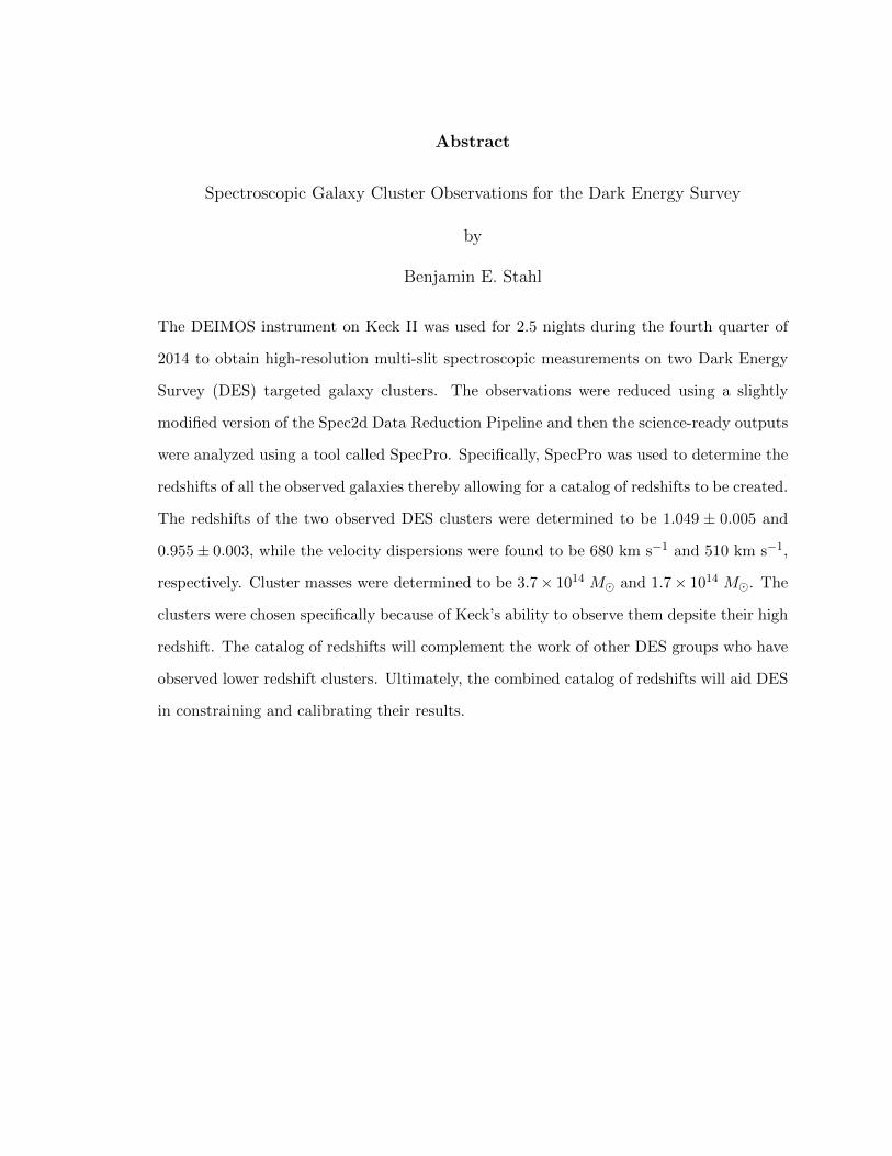
Abstract

Spectroscopic Galaxy Cluster Observations for the Dark Energy Survey

by

Benjamin E. Stahl

The DEIMOS instrument on Keck II was used for 2.5 nights during the fourth quarter of

2014 to obtain high-resolution multi-slit spectroscopic measurements on two Dark Energy

Survey (DES) targeted galaxy clusters. The observations were reduced using a slightly

modified version of the Spec2d Data Reduction Pipeline and then the science-ready outputs

were analyzed using a tool called SpecPro. Specifically, SpecPro was used to determine the

redshifts of all the observed galaxies thereby allowing for a catalog of redshifts to be created.

The redshifts of the two observed DES clusters were determined to be 1.049 ± 0.005 and

0.955 ± 0.003, while the velocity dispersions were found to be 680 km s−1 and 510 km s−1,

respectively. Cluster masses were determined to be 3.7× 1014 M and 1.7× 1014 M. The

clusters were chosen specifically because of Keck’s ability to observe them depsite their high

redshift. The catalog of redshifts will complement the work of other DES groups who have

observed lower redshift clusters. Ultimately, the combined catalog of redshifts will aid DES

in constraining and calibrating their results.

iv

Contents

List of Figures v

List of Tables vi

Acknowledgements vii

1 Introduction 1

2 Observations 42.1 Experimental Apparatus . . . . . . . . . . . . . . . . . . . . . . . . . . . . . 42.2 Calibration & Set Up . . . . . . . . . . . . . . . . . . . . . . . . . . . . . . . 42.3 Science Data Collection . . . . . . . . . . . . . . . . . . . . . . . . . . . . . 5

3 Data 63.1 Spec2d Data Reduction Pipeline . . . . . . . . . . . . . . . . . . . . . . . . 6

3.1.1 Spec2d Version and Modifications . . . . . . . . . . . . . . . . . . . 73.1.2 Plan File . . . . . . . . . . . . . . . . . . . . . . . . . . . . . . . . . 73.1.3 Reduction Process . . . . . . . . . . . . . . . . . . . . . . . . . . . . 8

3.2 Preparation for Analysis . . . . . . . . . . . . . . . . . . . . . . . . . . . . . 10

4 Analysis & Results 114.1 Redshift . . . . . . . . . . . . . . . . . . . . . . . . . . . . . . . . . . . . . . 11

4.1.1 Redshift Determination . . . . . . . . . . . . . . . . . . . . . . . . . 114.1.2 Redshift Results . . . . . . . . . . . . . . . . . . . . . . . . . . . . . 13

4.2 Velocity Dispersion . . . . . . . . . . . . . . . . . . . . . . . . . . . . . . . . 184.3 Cluster Mass . . . . . . . . . . . . . . . . . . . . . . . . . . . . . . . . . . . 18

5 Discussion 19

A Spec2d Modifications 21

B Sample Plan File 22

Bibliography 23

v

List of Figures

3.1 Numbering scheme for the chips in the DEIMOS CCD array as used by theSpec2d Data Reduction Pipeline [13]. . . . . . . . . . . . . . . . . . . . . . . 7

3.2 Arc lamp spectra mapped to four rectangular arrays corresponding to slitletsin the slitmask ‘0223 2’. . . . . . . . . . . . . . . . . . . . . . . . . . . . . . 9

4.1 Screenshot of the SpecPro tool in use analyzing the spectra of a DES0223-0416 member galaxy. The top graph shows the one-dimensional galaxy spec-trum and the bottom shows the two-dimensional spectrum that it was ex-tracted from. Overlayed on the one-dimensional spectrum in magenta is thebest fit of the VVDS S0 template, giving the result of z = 1.043 ± 0.0007.Addionally, specific spectral lines such as OII emission and Ca H, Ca K, andG-band absorption are overlayed to verify the fit of the model to the truespectrum. In the two-dimensional spectrum there is an obvious serendipitousspectrum showing several strong emission features in addition to the that ofthe desired target. . . . . . . . . . . . . . . . . . . . . . . . . . . . . . . . . 13

4.2 The left histogram contains all redshifts of the galaxies observed for DES0223-0416 that were given a quality rating of 3. The histogram on the rightcontains the subset of these galaxies that are suspected member-galaxieswith a fitted Gaussian overlayed. . . . . . . . . . . . . . . . . . . . . . . . . 17

4.3 Histograms of the redshifts of the galaxies observed for DES0215-0458 fol-lowing the same convention as in Figure 4.2. . . . . . . . . . . . . . . . . . . 17

vi

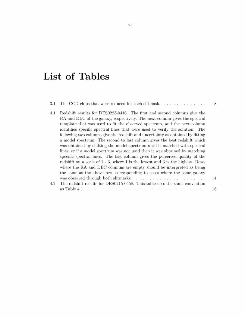
List of Tables

3.1 The CCD chips that were reduced for each slitmask. . . . . . . . . . . . . . 8

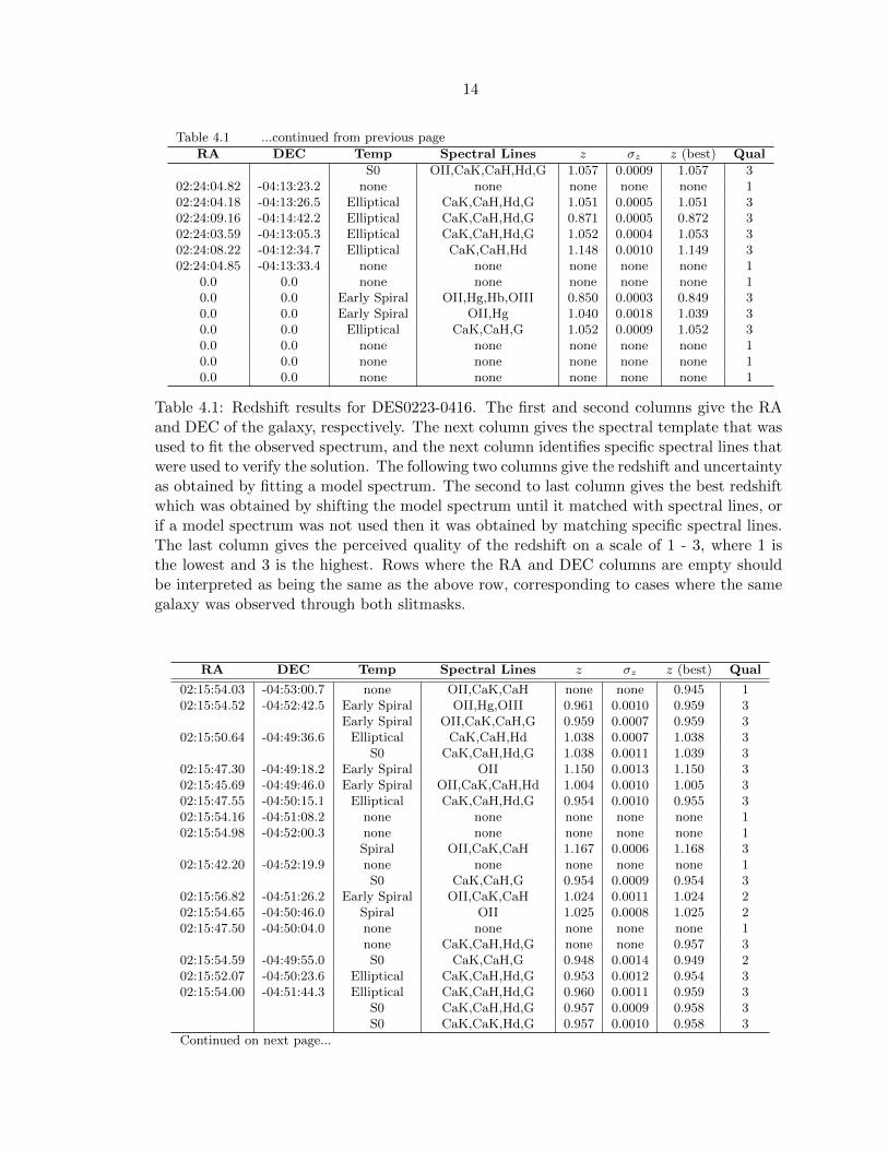
4.1 Redshift results for DES0223-0416. The first and second columns give theRA and DEC of the galaxy, respectively. The next column gives the spectraltemplate that was used to fit the observed spectrum, and the next columnidentifies specific spectral lines that were used to verify the solution. Thefollowing two columns give the redshift and uncertainty as obtained by fittinga model spectrum. The second to last column gives the best redshift whichwas obtained by shifting the model spectrum until it matched with spectrallines, or if a model spectrum was not used then it was obtained by matchingspecific spectral lines. The last column gives the perceived quality of theredshift on a scale of 1 - 3, where 1 is the lowest and 3 is the highest. Rowswhere the RA and DEC columns are empty should be interpreted as beingthe same as the above row, corresponding to cases where the same galaxywas observed through both slitmasks. . . . . . . . . . . . . . . . . . . . . . 14

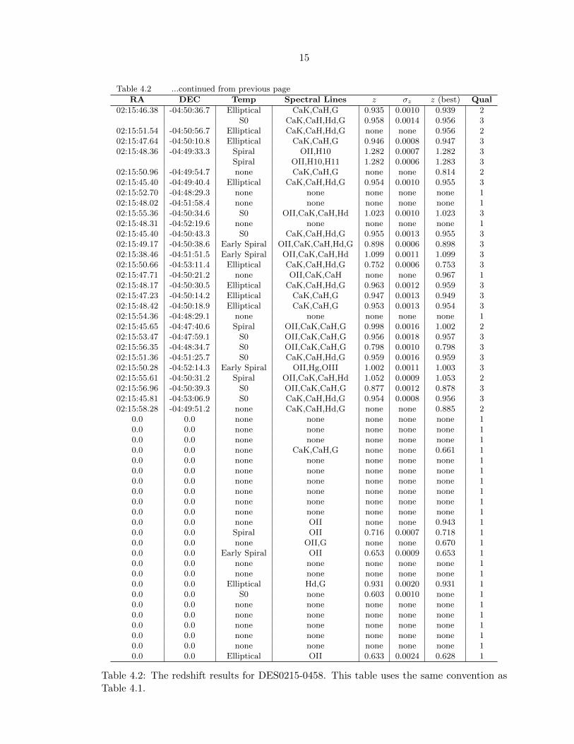
4.2 The redshift results for DES0215-0458. This table uses the same conventionas Table 4.1. . . . . . . . . . . . . . . . . . . . . . . . . . . . . . . . . . . . 15

vii

Acknowledgements

The project presented in this paper would not have been possible without the mentorship,

encouragement, and support of the following people and organizations:

I would like to thank my advisor, Professor Tesla Jeltema, for mentoring me and including

me in her research activities. She helped to define this project for me and really gave me

the freedom to learn and develop my research skills. I am also grateful to her for bringing

me along to Keck in Hawaii for the data collection, and for giving such timely and useful

feedback on the drafts of this thesis. I would like to thank Devon Hollowood for assisting

in the observations and for helping me sort through code and computer issues as they arose

in my work. Dr Bradford Holden also spent many hours meeting with me to help address

problems arising during the reduction of the data. Special thanks go to Michael Cooper

who illuminated and shared the solution to the problem of incorrect wavelength solutions

during data reduction.

This project was supported by funds from the National Science Foundation, the Department

of Energy, and the UCSC Undergraduate Research in Sciences Award.

1

1

Introduction

Current cosmological observations suggest that there is an energy associated with otherwise

empty space on all length scales. Without this ‘Dark Energy’, cosmological theories cannot

successfully explain why the Universe is flat, nor can they explain a host of bizarre effects

that are readily observed such as the fact that the Universe is not only expanding, but

accelerating in its expansion [5]. Alternative explanations have been proposed to account

for these effects, such as the assertion that general relativity may not be accurate on scales

larger than superclusters of galaxies. However, it is broadly held that new physics - the

Dark Energy - will be required to fully explain the observations.

One proposed form for Dark Energy is a scalar field such as quintessence, which is a dynamic

quantity whose energy density need not be constant in space and time. A simpler solution

is a cosmological constant (Λ); this leads to the Lambda Cold Dark Matter (ΛCDM) model,

which is currently the most utilized cosmological theory. The cosmological constant is the

energy density of the vacuum (i.e. empty space) and is uniform throughout space. The

idea was first introduced in 1917 by Einstein to counteract the effects of gravity and make

the Universe static. However, in 1929 Edwin Hubble discovered that all galaxies outside

of the Local group are moving away from one another, thus suggesting that the Universe

is expanding as a whole [4]. Common scientific lore claims that Einstein thought of his

2

cosmological constant as his biggest mistake. Hubble’s discovery led to a paradigm lasting

until the 1990’s that assumed the cosmological constant was zero. In 1998 however, ob-

servations of the relation between distance and redshift (z) for Type Ia supernovae were

published showing that the expansion of the Universe is accelerating [8] [10]. Since these

astonishing results were published, evidence for this ‘cosmic acceleration’ has been found in

measurements of the cosmic microwave background by the WMAP and Planck satellites,

as well as from a host of other sources.

ΛCDM successfully explains these observations and also predicts that Dark Energy is very

homogeneous and extremely low density (∼ 10−30 g/cm3 on mass-energy equivalence ba-

sis) [2]. With such a low density, Dark Energy is likely undetectable in a standard laboratory

experiment and is also not expected to interact with any of the fundamental forces of nature

except for gravity. Dark Energy has an enormous effect on the Universe only because it

uniformly fills all of space. Current results suggest that Dark Energy accounts for 68.3%

of the mass-energy density of the Universe, that Dark Matter accounts for 26.8%, and that

the remaining 4.9% is in ordinary baryonic matter [9].

On the forefront of current observational studies into Dark Energy is an international col-

laboration known as the Dark Energy Survey (DES). Photometric data collection of a 5000

deg2 patch of the Southern sky was commenced by DES in September 2013 as part of a 5

year mission that aims to study the nature of Dark Energy in unprecedented quantitative

detail [12]. DES will use the following four methods to study the nature of Dark Energy:

• Counting galaxy clusters and measuring their spatial distribution at 0 < z < 1.

• Weak lensing on redshift shells up to z ∼ 1.

• Baryon acoustic oscillations.

• Type Ia supernovae at 0.3 < z < 0.8.

Clearly, redshift plays an important role in the methods of the survey and will be funda-

3

mental to some of the studies. Redshift is so integral because it encodes a vast amount of

information about an object including notions of age, distance, velocity, and so on. Given

the relevance, photometric redshifts will be included in DES data products. Such redshifts,

which are calculated from the flux in a handful of photometric filters, are inherently impre-

cise compared to those that are calculated from spectroscopic observations. However, the

technique of photometric redshifts is much more efficient in terms of telescope time, and is

suited to the vast number of observations that DES is making.

Most of the scientific goals of DES will not be hindered by the lower precision, but a

dominant source of systematic error in their galaxy cluster program of study will be the de-

termination of the mass of a cluster [12]. As such there is a need to probe and quantify the

systematic errors as well as calibrate a mass-observable relation. For DES this observable is

cluster richness, which is essentially a measure of the number of member galaxies in a clus-

ter. In order to calibrate the richness-mass relation, two DES galaxy clusters were selected

for follow up spectroscopic observations that will allow for the redshift of member galaxies

and subsequently through dynamics, the mass of each observed cluster to be determined

to a high level of precision. These clusters were chosen specifically for observation on Keck

because their high redshifts (z ∼ 1) make them difficult to observe with other telescopes.

The spectroscopic redshift determinations discussed in this paper will be added to larger

samples of lower redshift clusters that have been observed by other DES groups, which will

ultimately allow DES to constain and calibrate their photometric redshifts.

These follow up spectroscopic observations and the related analysis form the basis of the sci-

entific project detailed in this paper. High resolution spectroscopic measurements of galaxies

within two DES clusters were made at the W.M. Keck Observatory. These observations

were then used to determine the redshift and mass of the clusters. This was accomplished

by completing a series of objectives leading from experimental design, to observation, to

data reduction, to analysis, and ultimately to a conclusion.

4

2

Observations

2.1 Experimental Apparatus

Experimental data was taken using the following instruments and equipment:

Telescope: Keck II 10 m reflecting telescope located at the summit of Mauna Kea, Hawaii.

Detector: Deep Imaging Multi-Object Spectrograph (DEIMOS) [15].

• 8k x 8k detector mosaic utilizing eight MIT/Lincoln Labs CCDs1.

• Located at Nasmyth focus of Keck II

• Slitmasks2: 0223 1, 0223 2, DES215B, DES215 B, & DES215 3

• Grating: 1200G (1200 lines/mm)

• Filter: OG550

2.2 Calibration & Set Up

A total of three observing sessions were completed using the experimental apparatus de-

scribed in Section 2.1. The first session was conducted remotely from the UCSC remote

observations room in the basement of the Natural Sciences building during the second half

1Each of the CCDs is 2k x 4k.2Cluster DES0223-0416 was observed with 0223 1 & 0223 2, DES0215-0458 was observed with the others.

5

of the night of September 21, 2014. The remaining two sessions were conducted from the

W.M. Keck Observatory control room in Waimea, Hawaii on back-to-back full nights start-

ing on October 23, 2014. For each observing session regardless of where the observations

were conducted, the set up and calibration procedures in the DEIMOS manual were fol-

lowed and will be briefly outlined now3 [14].

First the remote desktop software that allows for the instrument to be manipulated and

controlled was started and then the status of DEIMOS was checked. Once reporting ready,

it was started up and then it was verified that the correct slitmasks, gratings, and filters

were in place for the observing run. Next, a test exposure was taken and then a series

of tasks were completed to align the slitmasks to be used during the observing session.

Then a series of exposures were taken to focus the instrument. The flexure compensation

system (FCS) was calibrated. Finally, calibration exposures were taken to later allow for

instrumental bias to be removed from the data. These included internal flat field and arc

lamp4 exposures. Upon completion of these exposures and all of the other intricacies in the

DEIMOS manual, the apparatus was considered ready for scientific data collection.

2.3 Science Data Collection

After completing the calibration and set up procedures as prescribed in Section 2.2 prior

to each session of observation, scientific data collection was commenced. The telescope was

pointed to the coordinates of the target, guiding was enabled, and then a sequence of 30

minute exposures were taken. On the half night, slitmask ‘0223 2’ was used with six science

exposures, then on the first full night (October 23, 2014), slitmasks ‘0223 1’ (6 science

exposures) and ‘DES215B’ (7 science exposures) were used for observing. During the final

session on the following night, the ‘DES215 B’ (6 science exposures) and ‘DES215 3’ (7

science exposures) masks were used for observation.

3It should be noted that the observer using the instrument for the first half of the night preceding thefirst observing session conducted these procures, while the author and collaborators of this paper conductedthe procedures on both of the full night observing sessions.

4The arc lamp exposures were taken with the following arc lamps activated: Kr, Xe, Ar, & Ne.

6

3

Data

Having successfully completed 3 observing sessions in which 5 slit masks were used in the

collection of spectroscopic measurements of the galaxies within two galaxy clusters targeted

by DES, the process of reducing the raw data was then commenced. The process by which

this data reduction, which converted the raw multi-slit spectral images into science ready

data products, was accomplished will be detailed in the following sections.

3.1 Spec2d Data Reduction Pipeline

The bulk of the data reduction process was accomplished using an existing suite of IDL

routines known as the Spec2d Data Reduction Pipeline [3] [7]. This pipeline was developed

for the DEEP2 Galaxy Redshift Survey, which used ∼ 90 nights of observing time on

DEIMOS to collect over 50,000 spectra of galaxies at z ∼ 1. Given that the pipeline was

designed for reducing two-dimensional spectra taken with DEIMOS (and specifically the

1200 line/mm grating) of galaxies at comparable redshifts to those that were observed for

this paper, the Spec2d pipeline was a natural choice for data reduction. The process by

which the pipeline was used to reduce the raw two-dimensional spectra that were obtained

during the observing sessions will be detailed in the following subsections.

7

3.1.1 Spec2d Version and Modifications

Changes to the DEIMOS instrument over the years have made the original pipeline employed

by the DEEP2 team prone to failures. Specifically, a failure mode in which an incorrect

wavelength solution is obtained was experienced during the reduction of the observations

presented in this paper. To rectify the problem, the beta version of the pipline was used

with some slight modifications to the code, which are detailed in Appendix A.

3.1.2 Plan File

The first step in using the Spec2d data reduction pipeline is to create a plain-text file (with

the extension .plan) containing keywords and values that specify how and what data to

reduce. Creating the ‘plan file’, as it is called, can be completed in an automated fashion

by running the IDL routine deimos planfile.pro from an IDL session initiated in the

same directory as the raw data to be reduced. This automated method creates a plan file

that specifies the flat field frames, arc frames, and science frames associated with a given

mask as well as the mask and raw data directory. It also specifies the ‘poly’ wavelength

fitting scheme by default. The plan files that were used to reduce the collected data were

generated using this automated routine and then modified to select only specific CCDs

(chips) to perform the reduction on using the ‘CHIPS’ keyword. Given the configuration

of the CCD array (Figure 3.1) and the shape of the observed clusters, a given slitmask did

not necessarily have slits cut that would allow light to fall on all of the chips.

Figure 3.1: Numbering scheme for the chips in the DEIMOS CCD array as used by theSpec2d Data Reduction Pipeline [13].

Thus, the chips that had no light fall upon them were excluded from the reduction. Further,

8

due to challenges with the data reduction pipeline there were several additional chips that

were not reduced. Table 3.1 shows which chips were reduced for each mask:

Mask Chips

0223 1 3,70223 2 2,3,6,7

DES215B 2,6DES215 B 2,6DES215 3 2,3,6,7

Table 3.1: The CCD chips that were reduced for each slitmask.

Having created plan files1 for each slit mask with the desired chips specified following the

process detailed above, the observations were then run through the pipeline. This was

done by using a master program called domask.pro in a 32-bit IDL session that draws the

information from a specified plan file and then manages the data reduction process.

3.1.3 Reduction Process

The method of data reduction performed by the Spec2d Data Reduction Pipeline is exten-

sively detailed by Newman et al. (2013) but will be outlined now in the fashion that it was

used for the observations reported in this paper [7]. Note that in every step, each CCD is

treated separately.

1. calibSlit: The specified flat field frames are read in and processed to correct for pixel-

to-pixel response variations and reject cosmic rays. Then the slitlets are identified and

located. Next, the combined flat field frame for each chip is mapped into rectangular

arrays corresponding to each slitlet, effectively creating individual, rectangular flat

fields for each slitlet.

2. Pixel-to-Wavelength Solution: The arc frame(s) are read in and corrected for

pixel-to-pixel response variations. Next, a shift in the spatial direction between the

arc data and the original flat field is found using a cross correlation process. After

this, arc spectra for each slitlet are extracted and mapped into rectangular arrays

1A sample plan file is included in Appendix B.

9

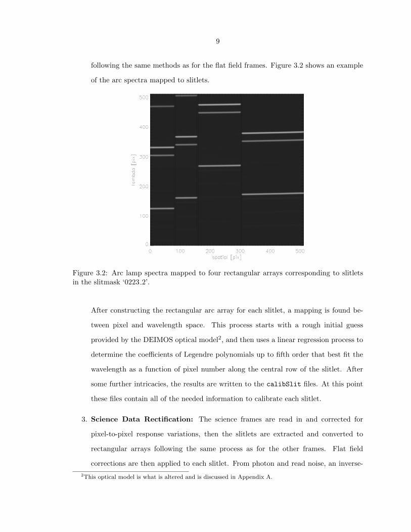
following the same methods as for the flat field frames. Figure 3.2 shows an example

of the arc spectra mapped to slitlets.

Figure 3.2: Arc lamp spectra mapped to four rectangular arrays corresponding to slitletsin the slitmask ‘0223 2’.

After constructing the rectangular arc array for each slitlet, a mapping is found be-

tween pixel and wavelength space. This process starts with a rough initial guess

provided by the DEIMOS optical model2, and then uses a linear regression process to

determine the coefficients of Legendre polynomials up to fifth order that best fit the

wavelength as a function of pixel number along the central row of the slitlet. After

some further intricacies, the results are written to the calibSlit files. At this point

these files contain all of the needed information to calibrate each slitlet.

3. Science Data Rectification: The science frames are read in and corrected for

pixel-to-pixel response variations, then the slitlets are extracted and converted to

rectangular arrays following the same process as for the other frames. Flat field

corrections are then applied to each slitlet. From photon and read noise, an inverse-

2This optical model is what is altered and is discussed in Appendix A.

10

variance image is also produced. Next, a B-spline model is used to fit the sky intensity

as a function of wavelength to the sky regions of each slitlet, thus allowing for sky

lines to be subtracted in the following step. At the completion of this step, a spSlit

file is written for each slitlet that contains the reduced 2D spectra from each science

frame as well as the other generated attributes.

4. Science 2D Spectra: In this step, the science exposures for each slitlet that were

generated in the previous step are combined into one inverse-variance weighted mean,

sky-subtracted, and cosmic ray rejected two dimensional spectrum. The result for

each slitlet is written into a slit file along with the wavelength solution and various

other information pertaining to the reduction. At this point, the two-dimensional

reduction is considered complete.

5. 1D Spectrum Extraction: In this final step, a one-dimensional science ready

spectrum is extracted from the completed and combined two-dimensional spectra

produced in the previous step. Multiple extraction methods are available, and the

default ‘optimal extraction’ method was utilized for all of the data being reported in

this paper. Each extracted one-dimensional spectrum is written to a spec1d file, even

if multiple objects fall on the same slitlet. In such cases where a spSlit file contains

more than one object, the pipeline produces a spec1d file for each object, and labels

suspected serendipitous objects in the file name.

3.2 Preparation for Analysis

As will be discussed in the following sections, an interactive tool called SpecPro was used

to perform significant parts of the analysis such as redshift determination [6]. In order to

use this tool, the science ready products from the Spec2d Pipeline, namely the spec1d and

slit files, were converted using the Keck DEIMOS 1D/2D wrapper [1]. For convenience,

a Python script was written to automate the process of using the wrapper. This script can

be made available by contacting the author.

11

4

Analysis & Results

Having corrected and calibrated the science frames according to the methodologies described

in Section 3, a process of scientific analysis was conducted. The details of this analysis and

the results of it will be presented in the following sections.

4.1 Redshift

The first step in the scientific analysis was to calculate the redshift of each galaxy for

which a one-dimensional object spectrum was extracted. This was accomplished in a semi-

automated fashion that will be detailed in the following section, and then the results from

this analysis will be presented in the subsequent section.

4.1.1 Redshift Determination

The redshift of each observed galaxy was determined using an interactive IDL tool called

SpecPro. Presentation of the full functionality and methodology of SpecPro are deferred to

Masters et al. (2011), but the process by which the software was used to extract redshifts

for this paper will be detailed in the following steps. Prior to starting these steps, the data

must be in SpecPro format as discussed in Section 3.2.

1. Start Up: From a 32-bit IDL session the SpecPro tool is initiated fromt the prompt

by typing specpro, xxx, where xxx denotes the slit number to start on. This will

12

open the SpecPro utility in a new window, if there are multiple spectra for the same

slit (i.e. serendipitous spectra) then a dialog box will open that allows the user to

select which spectrum to use.

2. Configuration: While SpecPro can read in a total of five1 files for a given slit, only

the one and two dimensional spectra were used for the analysis being reported in

this paper. Next, the displayed one-dimensional spectrum was binned and smoothed2

to better visualize the features in the spectrum. Many additional adjustments are

possible, but these were the only ones made at this stage.

3. Model Fitting: After obtaining a good visual representation of the features in the

spectrum, the redshift is obtained by using SpecPro to run a cross-correlation between

a selected spectral template3. The six best fitting solutions are available for each model

that is fit to the spectrum. In infrequent cases where a reasonable fit could not be

obtained with a model, this step was skipped.

4. Verification & Adjustment: Once a solution for the redshift was selected from one

of the fitted models, a verification was performed by overlaying specific spectral lines

on top of the spectrum to verify that there was indeed absorption or emission where

it should be. Should the fit not be perfectly aligned, the model was offset along the

wavelength axis to line up more precisely with the observed spectrum and thus obtain

a more accurate redshift. If no model fitting was used, then the redshift was found

by matching known spectral lines to the observed spectrum.

5. Output: Although SpecPro does provide for output of the results, this feature was

not used because a more thorough accounting of the redshifts and the confidence in

them was desired. Thus for each slitlet, the previous three steps were performed (the

software need not be restarted for each slitlet) and the results for each slitlet were

recorded into a file that contained the results for all the slitlets in a given mask.

11D spectrum, 2D spectrum, stamp image, photometry, information.2Inverse variance weighted average in the vicinity of each pixel to reduce the noise.3The spectral templates that were used for cross-correlation were: VVDS Elliptical, VVDS S0, VVDS

Early Spiral, and VVDS Spiral.

13

Figure 4.1 shows the SpecPro tool in use and serves to illustrate how it was used to determine

the redshift a galaxy.

Figure 4.1: Screenshot of the SpecPro tool in use analyzing the spectra of a DES0223-0416 member galaxy. The top graph shows the one-dimensional galaxy spectrum and thebottom shows the two-dimensional spectrum that it was extracted from. Overlayed on theone-dimensional spectrum in magenta is the best fit of the VVDS S0 template, giving theresult of z = 1.043 ± 0.0007. Addionally, specific spectral lines such as OII emission andCa H, Ca K, and G-band absorption are overlayed to verify the fit of the model to the truespectrum. In the two-dimensional spectrum there is an obvious serendipitous spectrumshowing several strong emission features in addition to the that of the desired target.

4.1.2 Redshift Results

The redshift results obtained using the process described in Section 4.1.1 will be presented,

for each DES cluster, in the following tables which were created using a script4 that pulled

all of the pertinent information together from the results files and the original .fits files

which contained the RA and DEC of the targets.

RA DEC Temp Spectral Lines z σz z (best) Qual

02:24:03.73 -04:13:39.7 Elliptical CaK,CaH,Hd,G 1.051 0.0011 1.052 302:23:58.20 -04:14:20.9 S0 OII,CaK,CaH,G,OIII 1.043 0.0008 1.044 3

S0 OII,CaK,CaH,Hd,G 1.043 0.0007 1.043 302:24:01.87 -04:13:25.3 Elliptical CaK,CaH,Hd,G 1.040 0.0007 1.041 3

S0 CaK,CaH,Hd,G 1.040 0.0014 1.041 302:23:59.70 -04:13:22.1 Elliptical CaK,CaH,Hd,G 1.050 0.0006 1.050 302:24:03.84 -04:13:11.8 Elliptical CaK,CaH,G 1.047 0.0011 1.048 302:23:59.90 -04:12:35.3 Elliptical CaK,CaH,Hd,G 1.057 0.0010 1.057 3

Continued on next page...4This script was also used to format the data for typesetting and is available by contacting the author.

14

Table 4.1 ...continued from previous page

RA DEC Temp Spectral Lines z σz z (best) Qual

S0 OII,CaK,CaH,Hd,G 1.057 0.0009 1.057 302:24:04.82 -04:13:23.2 none none none none none 102:24:04.18 -04:13:26.5 Elliptical CaK,CaH,Hd,G 1.051 0.0005 1.051 302:24:09.16 -04:14:42.2 Elliptical CaK,CaH,Hd,G 0.871 0.0005 0.872 302:24:03.59 -04:13:05.3 Elliptical CaK,CaH,Hd,G 1.052 0.0004 1.053 302:24:08.22 -04:12:34.7 Elliptical CaK,CaH,Hd 1.148 0.0010 1.149 302:24:04.85 -04:13:33.4 none none none none none 1

0.0 0.0 none none none none none 10.0 0.0 Early Spiral OII,Hg,Hb,OIII 0.850 0.0003 0.849 30.0 0.0 Early Spiral OII,Hg 1.040 0.0018 1.039 30.0 0.0 Elliptical CaK,CaH,G 1.052 0.0009 1.052 30.0 0.0 none none none none none 10.0 0.0 none none none none none 10.0 0.0 none none none none none 1

Table 4.1: Redshift results for DES0223-0416. The first and second columns give the RAand DEC of the galaxy, respectively. The next column gives the spectral template that wasused to fit the observed spectrum, and the next column identifies specific spectral lines thatwere used to verify the solution. The following two columns give the redshift and uncertaintyas obtained by fitting a model spectrum. The second to last column gives the best redshiftwhich was obtained by shifting the model spectrum until it matched with spectral lines, orif a model spectrum was not used then it was obtained by matching specific spectral lines.The last column gives the perceived quality of the redshift on a scale of 1 - 3, where 1 isthe lowest and 3 is the highest. Rows where the RA and DEC columns are empty shouldbe interpreted as being the same as the above row, corresponding to cases where the samegalaxy was observed through both slitmasks.

RA DEC Temp Spectral Lines z σz z (best) Qual

02:15:54.03 -04:53:00.7 none OII,CaK,CaH none none 0.945 102:15:54.52 -04:52:42.5 Early Spiral OII,Hg,OIII 0.961 0.0010 0.959 3

Early Spiral OII,CaK,CaH,G 0.959 0.0007 0.959 302:15:50.64 -04:49:36.6 Elliptical CaK,CaH,Hd 1.038 0.0007 1.038 3

S0 CaK,CaH,Hd,G 1.038 0.0011 1.039 302:15:47.30 -04:49:18.2 Early Spiral OII 1.150 0.0013 1.150 302:15:45.69 -04:49:46.0 Early Spiral OII,CaK,CaH,Hd 1.004 0.0010 1.005 302:15:47.55 -04:50:15.1 Elliptical CaK,CaH,Hd,G 0.954 0.0010 0.955 302:15:54.16 -04:51:08.2 none none none none none 102:15:54.98 -04:52:00.3 none none none none none 1

Spiral OII,CaK,CaH 1.167 0.0006 1.168 302:15:42.20 -04:52:19.9 none none none none none 1

S0 CaK,CaH,G 0.954 0.0009 0.954 302:15:56.82 -04:51:26.2 Early Spiral OII,CaK,CaH 1.024 0.0011 1.024 202:15:54.65 -04:50:46.0 Spiral OII 1.025 0.0008 1.025 202:15:47.50 -04:50:04.0 none none none none none 1

none CaK,CaH,Hd,G none none 0.957 302:15:54.59 -04:49:55.0 S0 CaK,CaH,G 0.948 0.0014 0.949 202:15:52.07 -04:50:23.6 Elliptical CaK,CaH,Hd,G 0.953 0.0012 0.954 302:15:54.00 -04:51:44.3 Elliptical CaK,CaH,Hd,G 0.960 0.0011 0.959 3

S0 CaK,CaH,Hd,G 0.957 0.0009 0.958 3S0 CaK,CaK,Hd,G 0.957 0.0010 0.958 3

Continued on next page...

15

Table 4.2 ...continued from previous page

RA DEC Temp Spectral Lines z σz z (best) Qual

02:15:46.38 -04:50:36.7 Elliptical CaK,CaH,G 0.935 0.0010 0.939 2S0 CaK,CaH,Hd,G 0.958 0.0014 0.956 3

02:15:51.54 -04:50:56.7 Elliptical CaK,CaH,Hd,G none none 0.956 202:15:47.64 -04:50:10.8 Elliptical CaK,CaH,G 0.946 0.0008 0.947 302:15:48.36 -04:49:33.3 Spiral OII,H10 1.282 0.0007 1.282 3

Spiral OII,H10,H11 1.282 0.0006 1.283 302:15:50.96 -04:49:54.7 none CaK,CaH,G none none 0.814 202:15:45.40 -04:49:40.4 Elliptical CaK,CaH,Hd,G 0.954 0.0010 0.955 302:15:52.70 -04:48:29.3 none none none none none 102:15:48.02 -04:51:58.4 none none none none none 102:15:55.36 -04:50:34.6 S0 OII,CaK,CaH,Hd 1.023 0.0010 1.023 302:15:48.31 -04:52:19.6 none none none none none 102:15:45.40 -04:50:43.3 S0 CaK,CaH,Hd,G 0.955 0.0013 0.955 302:15:49.17 -04:50:38.6 Early Spiral OII,CaK,CaH,Hd,G 0.898 0.0006 0.898 302:15:38.46 -04:51:51.5 Early Spiral OII,CaK,CaH,Hd 1.099 0.0011 1.099 302:15:50.66 -04:53:11.4 Elliptical CaK,CaH,Hd,G 0.752 0.0006 0.753 302:15:47.71 -04:50:21.2 none OII,CaK,CaH none none 0.967 102:15:48.17 -04:50:30.5 Elliptical CaK,CaH,Hd,G 0.963 0.0012 0.959 302:15:47.23 -04:50:14.2 Elliptical CaK,CaH,G 0.947 0.0013 0.949 302:15:48.42 -04:50:18.9 Elliptical CaK,CaH,G 0.953 0.0013 0.954 302:15:54.36 -04:48:29.1 none none none none none 102:15:45.65 -04:47:40.6 Spiral OII,CaK,CaH,G 0.998 0.0016 1.002 202:15:53.47 -04:47:59.1 S0 OII,CaK,CaH,G 0.956 0.0018 0.957 302:15:56.35 -04:48:34.7 S0 OII,CaK,CaH,G 0.798 0.0010 0.798 302:15:51.36 -04:51:25.7 S0 CaK,CaH,Hd,G 0.959 0.0016 0.959 302:15:50.28 -04:52:14.3 Early Spiral OII,Hg,OIII 1.002 0.0011 1.003 302:15:55.61 -04:50:31.2 Spiral OII,CaK,CaH,Hd 1.052 0.0009 1.053 202:15:56.96 -04:50:39.3 S0 OII,CaK,CaH,G 0.877 0.0012 0.878 302:15:45.81 -04:53:06.9 S0 CaK,CaH,Hd,G 0.954 0.0008 0.956 302:15:58.28 -04:49:51.2 none CaK,CaH,Hd,G none none 0.885 2

0.0 0.0 none none none none none 10.0 0.0 none none none none none 10.0 0.0 none none none none none 10.0 0.0 none CaK,CaH,G none none 0.661 10.0 0.0 none none none none none 10.0 0.0 none none none none none 10.0 0.0 none none none none none 10.0 0.0 none none none none none 10.0 0.0 none none none none none 10.0 0.0 none none none none none 10.0 0.0 none OII none none 0.943 10.0 0.0 Spiral OII 0.716 0.0007 0.718 10.0 0.0 none OII,G none none 0.670 10.0 0.0 Early Spiral OII 0.653 0.0009 0.653 10.0 0.0 none none none none none 10.0 0.0 none none none none none 10.0 0.0 Elliptical Hd,G 0.931 0.0020 0.931 10.0 0.0 S0 none 0.603 0.0010 none 10.0 0.0 none none none none none 10.0 0.0 none none none none none 10.0 0.0 none none none none none 10.0 0.0 none none none none none 10.0 0.0 none none none none none 10.0 0.0 Elliptical OII 0.633 0.0024 0.628 1

Table 4.2: The redshift results for DES0215-0458. This table uses the same convention asTable 4.1.

16

In the results presented in Tables 4.1 & 4.2, there are some rows where the RA and DEC

have the value of 0.0, these are all serendipitous galaxies that happened to be observed

through the slits, but were not the intended targets of observation. Any trustworthy red-

shifts obtained from these will be used, but they are quite likely to be non-member galaxies.

Fields in the table that have ‘none’ simply mean that nothing was used or obtained, depend-

ing on the context. For example, a very small number of the spectra had bad wavelength

solutions, others had no discernable spectral features, others couldn’t be fit with a model

spectrum but had clearly visible features that were used to measure the redshift. Also,

some of the serendipitous galaxies ‘found’ by the pipeline were on the edge of a slit making

them either an artifact of the reduction process or having a signal-to-noise ratio that was

too low. The ranking scheme of 1 - 3 was employed to distinguish trustworthy spectra from

questionable or clearly erronious cases. A rating of 1 was used in any case where there was

a bad wavelength solution, no spectral features, or it was clear that there was a problem

during the data reduction. 2 was used when the fitted model had to be shifted substantially

to line up, or when the fit looked reasonable but not dead on. Cases where the model fitting

lined up tightly, or where only a very minor offset was needed to make the spectral features

line up were given a rating of 3. As can be seen in the above tables, several galaxies where

observed more than once due to the multiple slitmasks that were employed in observing

each of the two clusters. In cases where trustworthy (quality = 3) redshifts are obtained,

they agree very well. Additionally, in cases where one slit mask failed to provide a good ob-

servation of one galaxy, the other often did yield a good observation, and ultimately redshift.

To better visualize the distribution of trustworthy redshifts for each of the two DES clusters

that were observed, the z (best) results were used to construct histograms. These histograms

contain only the redshifts given a quality rating of 3, and cases where the same galaxy was

observed more than once were treated by taking the mean of all measured redshifts for the

galaxy thereby preventing any over-counting.

17

0.80 0.85 0.90 0.95 1.00 1.05 1.10 1.15z

0

1

2

3

4

5

6

Occ

ure

nce

s

1.040 1.045 1.050 1.055 1.060z

0.0

0.5

1.0

1.5

2.0

2.5

3.0

3.5

4.0

4.5

µz = 1.050σz = 0.005

Figure 4.2: The left histogram contains all redshifts of the galaxies observed for DES0223-0416 that were given a quality rating of 3. The histogram on the right contains the subsetof these galaxies that are suspected member-galaxies with a fitted Gaussian overlayed.

0.7 0.8 0.9 1.0 1.1 1.2 1.3z

0

2

4

6

8

10

12

Occ

ure

nce

s

0.940 0.945 0.950 0.955 0.960 0.965 0.970z

0

1

2

3

4

5

6

7

8

µz = 0.955σz = 0.003

Figure 4.3: Histograms of the redshifts of the galaxies observed for DES0215-0458 followingthe same convention as in Figure 4.2.

The suspected member galaxies that are referenced in the right histograms from the above

figures are simply those that were grouped tightly (from a visual inspection) about the

highest bin in the left histogram for each figure. In the case of Figure 4.2 this range was

1.05 < z < 1.06 and for Figure 4.3 it was 0.94 < z < 0.97. The mean and standard deviation

of the redshifts of the suspected member galaxies were taken for each cluster and then used

to overplot the fitted Gaussians shown in the above figures, in this paper these means will

be considered to be the central redshift of each cluster. The redshift of DES0223-0416 was

18

found to be 1.049 ± 0.005 and for DES0215-0458 it was found to be 0.955 ± 0.003.

4.2 Velocity Dispersion

After obtaining the redshift catalog given in Tables 4.1 & 4.2, the proper velocities, vi, of the

suspected member galaxies were obtained for each cluster using the following equation [11]:

vi =zi − z

1 + zc (4.1)

Where zi is the member galaxy redshift, z is the mean redshift for the cluster, and c is the

speed of light.

After performing this calculation for each member galaxy in a cluster, the standard deviation

was taken. This result is called the velocity dispersion, σr. Using this methodology, the

velocity dispersion for DES0223-0416 was found to be 680 km s−1 and for DES0215-0458 it

was found to be 510 km s−1.

4.3 Cluster Mass

The mass of each cluster will be found using the following scaling relation [11]:

M ≈(

σr939z0.33

)2.91

1015M (4.2)

Performing this calculation for each cluster reveals that the mass of DES0223-0416 is approx-

imately 3.7×1014 M and that the mass of DES0215-0458 is approximately 1.7×1014 M.

19

5

Discussion

This paper presents high-resolution multi-slit spectroscopic observations made on two high

redshift DES targeted galaxy clusters and the results obtained from them. The observations

were collected over multiple nights using the DEIMOS instrument on Keck II at the W.M.

Keck Observatory. The pre-existing Spec2d Data Reduction Pipeline was used, with mod-

ification, to reduce the raw data into science-ready one and two-dimensional spectra of the

galaxies in each of the two observed clusters. The science-ready spectra were then analyzed

with the aid of a tool called SpecPro to determine the redshifts of all of the observed galaxies.

For DES0223-0416, a total of 22 spectra were studied with SpecPro. Of these, a total of 13

unique1, quality redshifts were obtained and of these 9 are from suspected member galaxies.

In the case of DES0215-0458, a total of 76 spectra were studied. After averaging together

multiple observations of the same galaxy and rejecting low quality spectra there are 28

unique, quality redshifts of which 16 are suspected to be member galaxies.

By taking the mean of all the redshifts of the suspected member galaxies, the redshift

of DES0223-0416 was found to be 1.049 ± 0.005 and the redshift of DES0215-0458 to be

0.955±0.003. Using these results the velocity dispersion for DES0223-0416 was determined

to be 680 km s−1 and for DES0215-0458 it was found to be 510 km s−1. Finally, the masses of

1This counts galaxies observed through both slitmasks only once

20

DES0223-0416 and DES0215-0458 were calculated to be 3.7× 1014 M and 1.7× 1014 M,

respectively. The catalog of redshifts and the results obtained from it will be added to

catalogs of lower redshift clusters produced by other DES groups, ultimately leading to a

robust sample of redshifts that DES will use to constrain and calibrate their results.

21

Appendix A

Spec2d Modifications

The beta version of the Spec2d Data Reduction Pipeline was modified as follows:

In the deimos mask calibrate.pro routine after the call to deimos omodel (around line

300) the following code was added (the call to deimos omodel is also shown for reference):

; process optical model for this chip

model_lambda = deimos_omodel(chipno, slitcoords, arc_header)

nloop = n_elements(model_lambda)

for ii=0,nloop-1 do begin

if model_lambda[ii].lambda_y[0] gt 0 then begin

model_lambda[ii].lambda_y[0] = model_lambda[ii].lambda_y[0] + 50.

model_lambda[ii].lambda_y_top[0] = model_lambda[ii].lambda_y_top[0] + 50.

model_lambda[ii].lambda_y_bottom[0] = model_lambda[ii].lambda_y_bottom[0] + 50.

endif

endfor

nslits=total(model_lambda.xb gt 0 AND model_lambda.xt gt 0)

In essence, this alteration just moves the optical model guess for the wavelength solution

by 50 angstroms (in this case, though other guesses aside from 50 could be used).

22

Appendix B

Sample Plan File

The plan file (0223 2.plan) used to reduce mask ‘0223 2’ is shown below. Note that the

first two lines are note interpreted by domask.pro because of the escape character (#).

# Plan file auto-generated by deimos_planfile.pro Wed Apr 22 15:01:01 2015

# Grating: 1200G Grangle: 10.1388

MASK: 0223_2

RAWDATADIR: /DES_work/keck_obs/2014sep21/raw

CHIPS: 2,3,6,7

polyflag - use polyflag for fitting lambda

FLATNAME: d0921_0017.fits

FLATNAME: d0921_0018.fits

FLATNAME: d0921_0019.fits

FLATNAME: d0921_0020.fits

FLATNAME: d0921_0021.fits

FLATNAME: d0921_0022.fits

FLATNAME: d0921_0023.fits

FLATNAME: d0921_0024.fits

FLATNAME: d0921_0025.fits

FLATNAME: d0921_0026.fits

ARCNAME: d0921_0015.fits

ARCNAME: d0921_0016.fits

SCIENCENAME: d0921_0029.fits

SCIENCENAME: d0921_0030.fits

SCIENCENAME: d0921_0032.fits

SCIENCENAME: d0921_0033.fits

SCIENCENAME: d0921_0035.fits

SCIENCENAME: d0921_0036.fits

23

Bibliography

[1] Keck DEIMOS 1D/2D wrapper. Available: http://specpro.caltech.edu/specpro_

wrappers.html.

[2] S. Carroll. The Cosmological Constant. Living Rev. Relativity, 4, 2001.

[3] M. C. Cooper, J. A. Newman, M. Davis, D. P. Finkbeiner, and B. F. Gerke. spec2d:

DEEP2 DEIMOS Spectral Pipeline. Astrophysics Source Code Library, March 2012.

[4] Edwin Hubble. A Relation Between Distance and Radial Velocity Among Extra-

Galactic Nebulae. Proceedings of the National Academy of Sciences, 15(3):168–173,

1929.

[5] R. Kallosh and A. Linde. Dark Energy and the Fate of the Universe. JCA, 2:2, Feb

2003.

[6] D. Masters and P. Capak. SpecPro: An Interactive IDL Program for Viewing and

Analyzing Astronomical Spectra. PASP, 123:638–644, May 2011.

[7] J. A. Newman, M. C. Cooper, M. Davis, S. M. Faber, A. L. Coil, P. Guhathakurta,

D. C. Koo, A. C. Phillips, C. Conroy, A. A. Dutton, D. P. Finkbeiner, B. F. Gerke,

D. J. Rosario, B. J. Weiner, C. N. A. Willmer, R. Yan, J. J. Harker, S. A. Kassin,

N. P. Konidaris, K. Lai, D. S. Madgwick, K. G. Noeske, G. D. Wirth, A. J. Connolly,

N. Kaiser, E. N. Kirby, B. C. Lemaux, L. Lin, J. M. Lotz, G. A. Luppino, C. Marinoni,

D. J. Matthews, A. Metevier, and R. P. Schiavon. The DEEP2 Galaxy Redshift Survey:

Design, Observations, Data Reduction, and Redshifts. ApJS, 208:5, September 2013.

24

[8] S. Perlmutter, G. Aldering, G. Goldhaber, R. A. Knop, P. Nugent, P. G. Castro,

S. Deustua, S. Fabbro, A. Goobar, D. E. Groom, I. M. Hook, A. G. Kim, M. Y. Kim,

J. C. Lee, N. J. Nunes, R. Pain, C. R. Pennypacker, R. Quimby, C. Lidman, R. S.

Ellis, M. Irwin, R. G. McMahon, P. Ruiz-Lapuente, N. Walton, B. Schaefer, B. J.

Boyle, A. V. Filippenko, T. Matheson, A. S. Fruchter, N. Panagia, H. J. M. Newberg,

W. J. Couch, and T. S. C. Project. Measurements of Ω and Λ from 42 High-Redshift

Supernovae. ApJ, 517:565–586, June 1999.

[9] Planck Collaboration, P. A. R. Ade, N. Aghanim, M. I. R. Alves, C. Armitage-Caplan,

M. Arnaud, M. Ashdown, F. Atrio-Barandela, J. Aumont, H. Aussel, and et al. Planck

2013 results. I. Overview of products and scientific results. AAP, 571:A1, November

2014.

[10] A. G. Riess, A. V. Filippenko, P. Challis, A. Clocchiatti, A. Diercks, P. M. Garnavich,

R. L. Gilliland, C. J. Hogan, S. Jha, R. P. Kirshner, B. Leibundgut, M. M. Phillips,

D. Reiss, B. P. Schmidt, R. A. Schommer, R. C. Smith, J. Spyromilio, C. Stubbs, N. B.

Suntzeff, and J. Tonry. Observational Evidence from Supernovae for an Accelerating

Universe and a Cosmological Constant. AJ, 116:1009–1038, September 1998.

[11] J. Ruel, G. Bazin, M. Bayliss, M. Brodwin, R. J. Foley, B. Stalder, K. A. Aird, R. Arm-

strong, M. L. N. Ashby, M. Bautz, B. A. Benson, L. E. Bleem, S. Bocquet, J. E.

Carlstrom, C. L. Chang, S. C. Chapman, H. M. Cho, A. Clocchiatti, T. M. Craw-

ford, A. T. Crites, T. de Haan, S. Desai, M. A. Dobbs, J. P. Dudley, W. R. Forman,

E. M. George, M. D. Gladders, A. H. Gonzalez, N. W. Halverson, N. L. Harrington,

F. W. High, G. P. Holder, W. L. Holzapfel, J. D. Hrubes, C. Jones, M. Joy, R. Keisler,

L. Knox, A. T. Lee, E. M. Leitch, J. Liu, M. Lueker, D. Luong-Van, A. Mantz, D. P.

Marrone, M. McDonald, J. J. McMahon, J. Mehl, S. S. Meyer, L. Mocanu, J. J. Mohr,

T. E. Montroy, S. S. Murray, T. Natoli, D. Nurgaliev, S. Padin, T. Plagge, C. Pryke,

C. L. Reichardt, A. Rest, J. E. Ruhl, B. R. Saliwanchik, A. Saro, J. T. Sayre, K. K.

Schaffer, L. Shaw, E. Shirokoff, J. Song, R. Suhada, H. G. Spieler, S. A. Stanford,

25

Z. Staniszewski, A. A. Starsk, K. Story, C. W. Stubbs, A. van Engelen, K. Vander-

linde, J. D. Vieira, A. Vikhlinin, R. Williamson, O. Zahn, and A. Zenteno. Optical

Spectroscopy and Velocity Dispersions of Galaxy Clusters from the SPT-SZ Survey.

ApjJ, 792:45, September 2014.

[12] E Sanchez and the DES Collaboration. The Dark Energy Survey. Journal of Physics:

Conference Series, 259(1):012080, 2010.

[13] UC Irvine. DEEP2 Spec2d Cookbook. Available: http://deep.ps.uci.edu/spec2d/

cookbook.html.

[14] W.M. Keck Observatory, Mauna Kea, Hawaii. DEIMOS Afternoon Checklist. Avail-

able: http://www2.keck.hawaii.edu/inst/deimos/checklist-pm.html.

[15] W.M. Keck Observatory, Mauna Kea, Hawaii. DEIMOS Home Page. Available: http:

//www2.keck.hawaii.edu/inst/deimos/.