university library three essays on investment… · 2.2 tot effect in a simple intertemporal model...
TRANSCRIPT

UNIVERSITY OF HAWAI'I LIBRARY
THREE ESSAYS ON INVESTMENT, SAVING, AND THE CURRENT ACCOUNT
A DISSERTATION SUBMITTED TO THE GRADUATE DIVISION OF THE UNIVERSITY OF HAWAI'I IN PARTIAL FULFILLMENT OF THE
REQUIREMENTS FOR THE DEGREE OF
DOCTOR OF PHILOSOPHY
IN
ECONOMICS
AUGUST 2008
By
Xiaoming Wang
Dissertation Committee:
Byron Gangnes, Chairperson Sang-Hyop Lee Xiaojun Wang
nan Noy Cynthia Ning

We certify that we have read this dissertation and that, in our opinion, it is
satisfactory in scope and quality as a dissertation for the degree of Doctor of
Philosophy in Economics.
DISSERTATION COMMITTEE
ii

ABSTRACT
The purpose of this dissertation is to answer two major questions. First, can we
provide additional evidence pertaining the validity and usefulness of the intertempo-,
ral model of the current account? And second, if we say yes to the first question, how
will this model perform in the empirical studies related to macroeconomic factors,
such as investment and saving, that are closely related to the current account?
The first essay tests the intertemporal model of the current account in a large
country framework. Compared to the standard small country model co=only
used in the literature, our model shows that only country-specific component of net
income will affect the current account, and it generates smoother current account
series, implying a stronger connection between current consumption and current
net income. Subsequent comparative empirical studies of small- and large-country
models, done in the framework of a present value model, show that the large country
framework out-performs the traditional small country framework when the object
of interest is indeed a large country.
The second essay targets primarily the relationship between degree of persistence
of terms of trade (TOT) shock and the current account. Our major contribution is
to study this topic in a decomposition framework. To get a measure of the degree
of persistence, we use two decomposition techniques, Beveridge-Nelson decomposi
tion and HP filter, to decompose TOT into permanent and transitory components.
Empirical results show that the persistence of TOT shocks does play an important
role with respect to how the current account respond to such shocks.
The third essay investigates the relationship between investment and saving, or
the Feldstein-Horioka (FH) puzzle, by applying regular panel estimation models to
time series of investment and saving that are decomposed using a similar approach
iii

as in the second essay. Our empirical results confirm the findings of the earliel
work done using different econometric frameworks that short-run correlation is gen
erally much smaller than long-run correlation. Dependent on particular choice of
decomposition technique and panel model, we find some evidence that capital is
very mobile for OECD countries 1960-2004.
iv

Table of Contents
Abstract ...... . . . .. . . . . .. .. . . . . .. . .. .. .. . .. . . .. .. .. .. . .
List of Figures .. .. .. .. . . . . .. . . . .. .. .. .. . . .. . . .. . .. .. .. .. .. . . .
List of Tables ..... . .. .. .. .. .. .. .. . . .. . .. .. .. .. .. .. .. .. .. .. .. .. .. .. ..
1 Present Value Model of the Current Account in A General Equi-
librium Framework . . . . .
1.1 Introduction....
1.1.1 Background
1.1.2 Literature review
1.2 The Model. . . . . . . .
1.2.1 Two-country model with the same time preference. .
1.2.2 Two-country model with different time preferences .
1.3 Present value model: testing methodologies. . . .
1.4 Data and Estimation Results. .
1.5 Sensitivity Test . . . . . . . . .
1.5.1 Testing non-US G7 countries ...
1.5.2 Higher interest rate and sub-sample estimation.
v
.
iii
vii
viii
1
1
1
2
8
8
16
21
24
33
33
37

1.5.3 Quantitative comparison
1.6 Conclusion. ..
A.l Data Description
A.2 Mathematical Derivation of equations . .
A.2.1 Derivation of Eq.{1.6) ...... . ..
A.2.2 Derivation of the current account Eq.{1.9)
40
· .... 42
44
45
· . .. 45
.. .. 46
2 Permanent and Transitory Terms of Trade, Investment and the
Current Account ............................ 48
2.1 Introduction. . .. ........ . . . . . . . 48
2.2 TOT effect in a simple intertemporal model with investment . . .. 55
2.3 Empirical Results . . . .. ... . . . . . . . . .. 66
2.3.1 Data and dynamic features of productivity and TOT . . . .. 66
2.3.2 The simple model... ....... . . . . .. 69
2.3.3 The extended model
2.3.4 Sensitivity analysis
2.4 Conclusion. . . . .
B.l Derivation of Equations ...
B.1.1 Derivation of investment price index PI •.
B.1.2 Derivations of Eq.{2.5) and (2.6) ..
B.1.3 Derivation of Eq.{2.13) .....
B.1.4 Derivation of equation (2.18) .
B.1.5 Derivation of equation (2.19) .
B.2 Data Description .......... .
B.3 Beveridge-Nelson Decomposition ... .
vi
74
80
83
86
86
· . . .. 86
· .... 87
· .... 88
· . . . .. 90
· . . .. 91
· . . . .. 91

3 The Feldstein-Horioka Puzzle Revisited . . . . . . . . . . . . . . 96
3.1 Introduction . . . . " . . . 96
3.2 Three panel estimation models. . . .102
3.3 Data and some stylized facts . . . . .110
3.4 Empirical estimation . . . . . .114
3.4.1 A benchmark estimation . . . . .114
3.4.2 Estimation with decomposed series .114
3.4.3 Dynamics of long-run and short-run correlations . . . . . . . . 120
3.4.4 Comparing with other measures of short-run correlation .,. 126
3.5 Conclusion.................. ....
C.1 Blancard and Quah (BQ) decomposition model .
vii
. . 129
. .132

List of Figures
1.1 Volatility of consumption and net income. . . .
1.2 Volatility of the current account and net income
1.3 Volatility of consumption, p, and correlation between net incomes
1.4 Time series of the US current account as a percentage of GDP
1.5 Actual and in-sample predicted current account: 1889-2003 .
1.6 Composition of G7 economy by each country . .
1.7 Quantitative comparison of model performances
2.1 ~2 as a function of w and 'f/. • • • • • • • • . . .
2.2 The coefficient of terms of trade on investment equation
2.3 Relative importance of permanent and transitory TOT
2.4 Permanent and transitory terms of trade in the US ..
17
18
19
29
34
39
41
60
73
75
82
3.1 Empirical cumulative distribution function of t-statistics ....... 109
3.2 Time-averaged saving and investment for OECD countries: 1960-2004 111
3.3 Time properties of long-run and short-run correlations . 121
3.4 Comparing short-run correlations from different models .130
viii

List of Tables
1.1 Unit Root Tests . . .
1.2 Orthogonality Tests .
1.3 Wald test and ratio test ...
1.4 Statistical test performance of SOE and LOE models
27
31
32
42
2.1 Dynamic features of productivity and TOT. . . . . . . . . . . . . .. 68
2.2 Regression results: the simple model ............ 71
2.3 Regression results: the extended model with BN filter . 79
2.4 Regression results: the extended model with HP filler . 84
3.1 Monte Carlo simulation for panel regression ............ .. 107
3.2 Unit root and cointegration tests of investment and saving for 24
OECD countries. . . . . . . . . . . . . . . . . . . . . . . . .. ... 113
3.3 Investment-saving correlation for OECD countries: 1960-2004 ... 115
3.4 Unit root test of permanent and transitory investment and saving for
24 OECD countries . . . . . . . . . . . . . . . . . . . . . . .. ... 118
3.5 Differences between correlations with or without Luxembourg ... 123
3.6 Saving-investment correlations for 23 OECD countries 1960-2004: MG 125
ix

3.7 Saving-investment correlations for 23 OEOD countries 1960-2004:
PMG and EOM . . . . . . . . . . . . . . . . . . . . . . . . . . 128
x

Essay 1
Present Value Model of the
Current Account in A General
Equilibrium Framework
1.1 Introduction
1.1.1 Background
Since the early paper of Sachs (1981), the intertemporal approach has become a
popular and standard tool in studying the current account. It provides both mi
crofoundation and dynamics to the analysis. Intertemporal approach to the current
account is an extension of the permanent income hypothesis (PIH) in the consump
tion theory to an open economy framework. First introduced by Milton Friedman,
PIH states that a person will consume a constant proportion of permanent, instead
of current, income. The theory suggests that consumers will smooth their consump
tion spending based on the estimation of their permanent income, and they only
1
change their coIlSUIIlption profile when there exists a permanent shock to the real
income. In an open economy, the current account reflects the consequences of the
consumers' intertemporal cOIlSUIIlption-smoothing behavior. The current account
deterioration implies that the consumers' current income cannot meet their current
consumption need and therefore they borrow from foreign countries, whereas the
current account improvement suggests that the consumers are lending to the rest of
the world.
With simplifying assumptions, intertemporal approach yields an easily tractable
and analytical expression for the current account that can be conveniently tested
in a framework of present value model.1 Mathematically, the current account CA
can be expressed as the sum of all future expected net income (total output minus
govermnent expenditure and investment) changes !lN~, discounted at their present
values:
The model predicts that the current account will deteriorate (improve) when con
sumers expect their future net incomes to increase ( decrease).
1.1.2 Literature review
The present value model has been tested extensively in the literature. Earlier works
include Sheffrin and Woo (1990), Otto (1992), and Ghosh (1995). Because the model
is based on the assumption of a snian open economy (SOE), the world interest rate
is exogenously given and assumed to be constant. Sheffrin and Woo (1990) test the
present value model of the current account using amlUal data for four small industrial
1 For a good survey of the intertemporal approach to the current account, please refer to Obstfeld and Rogoff (1995).
2

countries (Belgium, Canada, Denmark, and UK) covering the period 1955-1985.
Different statistical testing methodologies provide mixed results for each country,
but Canada and UK are the most problematic, which gives momentum to various
later modifications of the bllBic intertemporal model so lIB to provide better fit. Using
data for both Canada and the US, Otto (1992) is the first one to test the present
value model with large country data. Surprisingly, the model faiis for both countries,
and does not perform better for Canada, which should have better statistical results
because the testable equations are designed bl!Bed upon SOE model and thus should
fit a small country, like Canada, better than a large one, like the US. In searching
for the possible rel!BOn for the statistical rejection, the author modifies the model
so that households get utility from government expenditure, but this alternative
assumption does not improve model performance. Ghosh (1995) finds that the SOE
model is rejected when using data from Japan, UK, Canada, and Germany, but not
for the case of the US. And for all rejections, the model predicted current accounts
are less variable than actual data, implying that the international capital is mobile.
Empirical studies in all three papers provide no statistical support for the validity
of the present value model of the current account (PVMCA) using data from ma.
jor industrial countries. The cross-equation restrictions that the standard PVMCA
imposes on the parameters of the unrestricted vector autoregression (VAR) are sta.
tistically rejected. And the model predicted current account is much less volatile
than that observed in actual data. Since current account is the difference between
net income and consumption, deficient current account volatility implies that the
model predicted consumption is too volatile.
To reduced the variability in consumption, a co=on modelling technique is to
include nonseparable preference (Sundaresan 1989). Later works on testing PVMCA
3

accommodate the assumption of nonseparability in different ways. !scan (1999) in
troduces durable and non-traded goods into the basic one-good model and tests it
against Canada data. The response of consumption to external shocks is dampened
because households need to keep a balanced combination of different goods. Ghosh
and Ostry (1997) find that the current account volatility can be increased if house
holds engage in precautionary saving. Gruber (2004) offers a solution to the excess
volatility problem by incorporating consumption habits into the standard model.
The optimal consumption depends not only on permanent income, but also on past
consumption. In response to net income shocks, the household tends to maintain
his past consumption level, leadinji; to a smoother consumption and a more volatile
current account.
An alternative way to improve the fit of the model is by allowing for variable
interest rate. Bergin and Sheffrin (2000) extend the basic present value model by
introducing variable interest rate and exchange rate. Using three small country
(Australia, Canada and UK) data, they find the modified model improves the fit
of the intertemporal model. Kano (2003) shows that a standard SOE real business
cycle model augmented with a stochastic world real interest rate can produce ob
servationallyequivalent result to the habit formation model in Gruber (2004), and
therefore he concludes that the future research on the current account should con
centrate on the determinants of the world interest rate rather than on alternative
specification of the utility function and preference.
Nason and Rogers (2003) conduct a comprehensive investigation into the possible
causes of statistical failure of PVMCA in a SOE real business cycle model. Besides
nonseparability and variable interest rate as observed earlier, they also present fiscal
shock and international capital immobility as potential explanations. Their simu-
4

lation results indicate that a model with exogenous interest rate shocks performs
best.
Since the interest rate plays an important role in validating the PVMCA, it
would be a natural question to ask what happeus to the current account dynamics
if the interest rate is not exogenously given, but endogenously determined in a two
country large open economy (LOE) framework. In this paper, we show that in a
general equilibrium framework the present value equation of the current account is
00
cat = - ErfEt(AYt+i - Ay~) 1=1
where A is the first difference operator, Y is the log form of domestic net output, yW
is the log form of world net output, and ca is Y minus c, the log form of domestic
consumption.
Obstfeld and Rogoff (1995) obtain a sinillar equation but in absolute, instead
of log, form. Without setting up a general equilibrium model, they make pre
assumption that the domestic net output can be decomposed into two parts, the
country-specific and the global parts, and that the global part affects the world
interest rate, but not the current account. Whereas in my approach, the world net
output is naturally derived as the weighted average of both home and foreign coun
tries, instead of being assumed to exist as a predetermined component of domestic
net output in an ad hoc way. That global shocks do not Inatter for the current
account is a conclusion naturally derived from my model.
With Obstfeld and Rogoff (1995) being a predecessor, this paper is not the first
one to show that the standard model can be modified to examine effects of global and
country-specific shocks on the current account, but it is the first one to present an
5
empirical study on the performance of this LOE intertemporal model in a traditional
present value framework,2 and make further comparison with the basic SOE model.
One major implication of the intertemporal approach is that global shocks will
not have any impact on the current account because all countries with symmetric
features respond to such disturbances analogously. With a positive shock, every
country will have the same intention to borrow in the international capital mar
ket. but no country wants to lend. The validity of such proposition, and therefore
of the intertemporal approach, is tested formally in Glick and Rogoff (1995). Basi
cally, they get estimates of country-specific and global technology shocks from Solow
residuals of individual countries and regress them against the current account vari
able. They find that the coefficient on the global shock is insignificant. Several later
works, including Iscan (2000), Bussiere, Fratzscher and Muller (2005), and Marquez
(2002) , follow their approach and find similar empirical results.
The SOE present value model caunot acco=odate such prediction because the
rest of the world, thus the global shock, is literally missing from the model structure.
The empirical estimations are mad.e without excluding global factors from domestic
net output variables, and therefore may be subject to errors. The LOE general
equilibrium framework, on the other hand, integrates Glick and Rogoff's (1995)
insight into a present value model that can be conveniently tested by following the
rationale and methodologies in a standard SOE model.
As observed earlier, a statistical finding co=on to all basic SOE present value
model papers is that with small industrial country data, the model predicted current
account is much less volatile than the actual data. This brings about the interest
'The only exception is a very recent paper by Engle and Rogers (2006), which models the current account, in a two-country framework, as the present value of the country's current and expected future shares of the world net output within a general equilibrium framework. But they did not forma11y test the validity of the present value model.
6

in later works to improve the fit of the model by introducing additional features.
What the literature fails to notice is that for all empirical tests done with the
US, the model predicted current account unanimously shows a larger volatility. In
Otto (1992), the model current account volatility is statistically greater than the
actual data, implying the rejection of the model. In Ghosh (1995), the model is
not rejected with US data, however the predicted current account is mathematically
more variable. In Gruber (2004), for both the US and Japan, a second largest
economy, the model underpredicts the volatility of actual current account even after
hahit formation is taken into consideration. Are these findings random or do they
indicate a systematic difference between large and small countries?
In this paper, we show that the LOE model would predict a smaller current
account volatility as compared to the SOE model, for which there exist two expla,
nations. First, the world interest rate is determined within the system. Therefore it
moves when home future net income changes. Household will unsmooth consump
tion by increasing( decreasing) current consumption relative to future consumption
when interest rate decreases(increases), making consumption more volatile than in
the case of SOE. Therefore, we would expect to see a drop in the volatility of the
current account.
The other reason is that in a two-country model, idiosyncratic shock to home
net income will more likely work in a way similar to a global shock which will
not have any effect on home current account, as pointed out by Glick and Rogoff
(1995). And this is especially true in current global environment when advances
in information technology spread quickly throughout the whole world and promote
economic growth.3 So we should also expect to have smaller predicted current
3Based on the same reason, Marquez (2002) tests the model of Glick and Rogoff (1995) using more recent data to study if current information technology advances have, more or less, changed
7

account volatility in the home country.
In the next section, we present a simple LOE intertemporal model. In section
3, we talk about empirical testing methodologies. In section 4 and 5, we report
detailed model testing results. Section 6 concludes.
1.2 The Model
1.2.1 Two-country model with the same time preference
Before we go into model details, let's first make clear variable definitions used in this
paper. For each home country variable X, we will have a foreign country counterpart
defined as X*. Low case x indicates log format of X, i.e. x = lnX. X indicates
steady state value of X, therfore x = lnX. Unless otherwise specified, all variables
will follow the above rules.
This is a two-country one-good world. The home representative agent tries to
maximize her life-time utility,
00
Ut = .L: ,Bs-tInG., s=t
subject to an intertemporal budget constraint,
Here Gt is consumption. ,B is time preference. Yi stands for net income, that is,
GDP minus investment and government expenditure, and is taken exogenous. Bt
is home country's net foreign assets. Tt is world real interest rate and determined
the way how productivity shocks affect current account dyuamics.
8

inside the system. The first order condition of maximizing problem is
(1.1)
By log-linearizing the above equation, we get
Llct+l = rt+1 + In,B (1.2)
where Llct+1 = InGt+l -InGt , rt+1 R; InCl +rt+1)' In steady state, consumption will
be constant, so ,B = t.!.;" and In,B R; -r. Assuming the foreign country has the same
time preference as in home country, we can write a similar Euler equation for the
foreign country
(1.3)
The world goods market clears when at any time t we have4
(1.4)
Using Eq. (Ll) and (1.3) to re-write the above equation as
(1.5)
'From Wa1ra's law, both bond market and goods market clear when one of them is cleared. So we only need to consider goods market clearing condition here.
5For simplicity, we assume home country and foreign country are of equal size in the sense of population. Adding a constant relative size parameter in the model only changes the resnlte marginally. For example, if the foreign country has a population n time that of the home country, the Eq. (1.6) will be Tt+1 = (1- *)AYt+1 + *AYt+1 -lnf3.
9

and do log-linearization (see appendix A.2.1 for details.)
(1.6)
where AYHl = lnytH - lnyt, AytH = lnY;~l - lnY;", and p = 1 + ef}-il". This
equation tells us that the world real interest rate actually is determined by the
weighted average of individual country's net income growth rate, or the world growth
rate. This implication is consistent with basic growth theory in which the real
interest rate is determined by population, which is omitted from the current model,
and technology growth rate, or general economic growth rate if we combine them
together.
To see the dynamics of consumption, we plug Eq.(1.6) into Eq.(1.2)
(1.7)
Standard SOE intertemporal model predicts that households smooth their consump
tion by solely referring to their expectation of all future incomes, or permanent net
income. In a circumstance without influences from income shocks, consumption pro
file will be rather flat, or following a random walk. In comparison, when we extend
to a two-country general equilibrium framework, the consumption growth tracks
the world growth rate closely and is proportional to home net income growth. The
reason is that consumption decision is made according to the current world interest
rate which is endogenously determined.
Empirically, low correlation between current consumption and current income,
as predicted by permanent income hypothesis, has been refuted by Campbell and
Shiller (1987). Theoretically, standard SOE intertemporal model is modified by
10

adding both saver- and spender-households to allow for larger connection between
current income and consumption (see Bussiere et al. (2005) for model details6). We
can see from the above equation that modelling the current acconnt in a general
equilibrium framework is another way to introduce the larger connection between
consumption and net income.
To derive dynamics of the current acconnt, we follow the methodology in Bergin
and Sheffrin (2000) by doing a log-linearization of the current acconnt equation and
the intertemporal budget constraint. The final result, the detailed derivation of
which can be found in appendix A.2.2, is
00
Ct = Yt + Elf Et( LlYt+i - Lly~), (1.8) 1=1
or
00
Cll.t - -ElfEt(LlYt+i - Lly~) (1.9) i=1 00
- -Elf EtLlyi+i' (1.10) i=1
where Cll.t = Yt - Ct, Lly'f = (1 - ~)LlYt + ~Lly;, and Llift = ~(LlYt - Llyt).
The equations we derived in appendix A.2.2 are under perfect foresight assump
tion without uncertainty, which is very unlikely in the real world. Therefore, we
simply take a short-cut by adding expectation operator into the right hand side of
the equations. These equations may not hold exactly if we had solved the problem
under uncertainty from the very beginning. But to make it mathematically simple,
we just take this as the true relationship between the expected future net incomes
6This framework was originally introduced by Campbell and Mankiw (1989) to test the perma.nent income hypothesis in consumption theory.
11

and the current account (consumption), and leave the concerns about errors in our
future research. Such a modelling technique haB also been taken by Iscan (1999)
and Engle and Rogers (2006).
Eq.(1.9) is analogous to the current account equation in a SOE PVMCA, except
that we have replaced the change of home net income with the relative, or country
specific component of, change in home net income (AYt - Ayf). Besides, the world
real interest rate drops off because it haB been solved out. This condition says that
what matters for the movement of the current account is the idiosyncratic part of
net income change whereaB the global part co=on to both countries does not have
effect.
We write down some baBic equations for a canonical SOE model and compare
them with what we have got from a LOE model. All notations, with a superscript
's' to represent SOE results, are of the same definition aB in the previous part of
the paper unless otherwise defined. These equations, all in log format for easy
comparison, are Euler equation
cousumption dynamics 00
c: = ift + L:.& Et(Aift+i) , i=1
and the current account dynamics
00
ca: = - L:'&Et(AY:+i)' '=1
12

Comparative statistics for the SOE model are:
8ct . r -=I-j3=-8yf l+r'
The majority of the adjustment of a temporary increase in domestic net income
occurs through the channel of an improvement in the current account while current
consumption only rises marginally (one for 1'::"). It is because the consumption is
smoothed intertemporally, so the change in consumption over time does not depend
on net income. Therefore the SOE model predicts that consumption should be much
less volatile than net income.
The comparative statistics in my model are:
8Ct 1 l8y; - = 1 - j3- + --, &ut p p8yt
P is defined as 1 + eY-il', so ~ is the share of foreign net income in global net income
in steady state, and 0 < ~ < 1. We can see that the temporary increase in net
income will have a larger effect on current consumption (1 - j3 < 1 - j3~) because
consumption dynamics is directly determined by the world interest rate which in
turn is endogenously determined by change in net income. Further, if the home net
income shock can be taken, to some extent, as a global shock, then we would expect
~ > O. So the effect of net income on cousumption will be even greater by the
amount of ~~. Putting everything together, in a general equilibrium framework,
consumption will be much less smoother than in a standard intertemporal model,
and we expect to see a larger consumption volatility together with a smaller current
account volatility.
To have a better and clearer picture about how different predictions these two
13
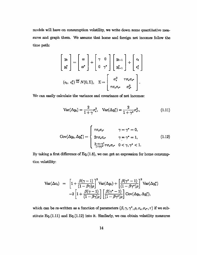
models will have on consumption volatility, we write down some quantitative mea
sures and graph them. We assume that home and foreign net incomes follow the
time path:
[ Yt 1 = [ a 1 + ['Y 0 1 [Yt_l 1 + [ €t 1 Y; a' 0 'Y' Yt-l e;
We can easily calculate the variance and covariance of net incomes:
Var(AYt) = -1 2 cr., Var(Ayn = 1 2 O'~., +'Y +"1'
(1.11)
(1.12)
By taking a first difference of Eq.(1.8), we can get an expression for home consump
tion volatility:
which can be re-written as a function of parameters ([3,'Y,'Y·,p,O'"O' •• ,r) if we sub-
stitute Eq.(1.11) and Eq.(1.12) into it. Similarly, we can obtain volatility measures
14

Var(Act) and Var(Ayt') for the SOE model, assuming net income follows a time
path with the same parameters ct, 'Y and error term ft.
In Figure 1.1, we show and compare four different cases. The x-axis is value
of" therefore with 'Y = 1, net income shock is permanent; 'Y = 0, transitory; and
o < 'Y < 1, the impact of net income shock is somewhere in between.
• SOE with constant interest rate (Ac, SOE). AB we can see, except for the
case with a permanent shock, consumption is much smoother than net income
(Ay), with only marginal oscillation. This is because households smooth their
consumption intertemporally, and make their consumption decisions based on
permanent, instead of current, net income.
• Large country with zero foreign net income shock and zero correlation between
home and foreign net incomes (Ac, LOE). Households make their consumption
decision based on the world real interest rate, which is determined by world
net income growth rate. Home net income shock will work on consumption
decision-making through the channel of interest rate. Compared with SOE
model, consumption is much more volatile.
• Large country with non-zerc foreign net income shock, but zero correlation
between home and foreign net incomes (Ac, LOE T = 0). Compared with the
second case, positive foreign net income shock, working on home consumption
decision through interest rate, adds volatility to consumption.
• Large country with non-zero foreign net income shock and non-zero correlation
between home and foreign net incomes (Ac, LOE T = O.S). With non-zero
correlation between net incomes, one country's net income shock can be taken,
to some degree, as a global shock, which shifts each country's consumption
15

profile without changing its current account. So consumption becomes even
more volatile if home country has a strong economic connection with the rest of
the world. And it is easy to see that consumption volatility profile shifts more
towards net income line when such correlation becomes larger. Consumption
and net income volatility lines coincide when correlation coefficient between
home and foreign net incomes is 1.
We can also graph the volatility of the current account under different cases, shown
in Figure 1.2. Clearly, the current account is expected to be much smoother for
large country than for small country, the reason of which, similar to that stated
above, will not be repeated here.
What also noticeable is the relationship between p and the volatility of consump
tion. As we said earlier, ~ is the steady state share of foreign net income in total
world net income. Home country becomes economically more important as p gets
larger. Same as correlation coefficient between home and foreign net incomes, a
larger p also tends to increase the volatility of home consumption. This is because
when home country takes a larger share of world economy, its idiosyncratic shock are
more likely to be taken as a global one. We show in Figure 1.3 that we expect to see
a larger consumption volatility with a larger value of either p or T, the correlation
coefficient between home and foreign net incomes.
1.2.2 Two-country model with different time preferences
When we have different time preferences for home and foreign countries, Euler equa
tion and market clearing condition will be different from Eq.(1.3) and Eq.(1.5), as
shown below:
(1.13)
16

1.8
1.6
1.4
12
Figure 1.1: Volatilio/ of consumption and net income
-4y --&:. LOE ...0.8 - - -&:. LOE...o ·-·-·&:.LOE ...... , Ac.SOE
f --- --- ,.. :> 0.8 - - - - _ _ ;/.,-----_ u: 0.6 - - - - - - - - - - ______ "" .,' -'- . . '_._._._._._._._._._._._._._._._._._._._._._._._._._., ;:
0.4
02
o •• """ '''', .. '',.".,'''' '"'' ", ..... ", .. ,"'" " .... " .... ,." .. , "" , ... " ......... ,.
Notes: This figure graphs and compares the volatilities of net income (Ay) and consumption in four different cases: the SOE with constant interest (Ac, SOE), the LOE with zero foreign net income shock and zero correlation between home and foreign net incomes (Ac, LOE), the LOE with non-zero foreign net income shock and zero correlation between home and foreign net incomes (Ac, LOE T = 0), and the LOE with non-zero foreign net income shock and non-zero correlation between home and foreign net incomes (Ac, LOE T = 0.8). All values are calculated sssurning con,1;ant time preference f3 = 0.96, or steady state interest rate if = 4%. p is assumed to be 2, or home and foreign each takes half of world total net income. Foreign net income is sssumed to take the same time path as home net income, 'i' = "I, and ~. = <T~ = 1.
17

Figure 1.2: Volatility of the current account and net income
2~----~----~----~~==~====~
1.8
1.6
1.4
1.2 ~
~ 1
0.8
0.6 0.4
...... ... -- ... -- --'-. -'-. -'-. -'-.-
-l1y --l1ca, LOE r-0.8 - - - I1ca, LOE r-O . _. - 'l1ca, LOE 'I" 1'1 Aca, SOE
--- --- -- ... ... ... '-'-'-' ... -.-.-. "'
0.2[==============-=·=-='~-~'~_~' ;;'i" J -..... , ...... ....... y ..
00 0.2 0.4 0.6 0.8 1 'Y
Notes: This figure graphs and compares the volatilities of net income (Ay) and the current account in four dilferent cases: the SOE with constant interest (Aca, SOE), the LOE with zero foreign net income shock and zero correlation between home and foreign net incomes (Aca, LOE), the LOE with non-zero foreign net income shock and zero correlation between home and foreign net incomes (Aca, LOE T = 0), and the LOE with non-zero foreign net income shock and non-zero correlation between home and foreign net incomes (Aca, LOE T = O.S). All values are calculated assuming constant time preference {3 = 0.96, or steady state interest rate If = 4%. p is assumed to be 2, or hOOle and foreign each takes half of world total net income. Foreign net income is assumed to take the same time path 88 home net income, 'Yo = 'Y, and cr.- = cr. = 1.
18

Figure 1.3: Volatility of consumption, p, and correlation between net incomes
1.3 -Ll.c. LOE ..... 0.p=1.8
1.2 - Ll.c. LOE ..... O.p=4 , - - - Ll.c. LOE ..... 0.8.p=1.8 , 1.1
, , , , 1
, , II
, ,
I 0.9 .... .... .... .... .... ....
0.8 .... .... .... .... .... .... 0.7 .... .... ....
0.6
0.5 0 0.2 0.4 0.6 0.8 1
r
Notes: This figure graphs and compares the volatilities of consumption in a LOE model in three different CIlBeS: T = 0 and p = 1.8, T = 0 and p = 4, T = 0.8 and p = 1.8, where p is the corre1ation between domestic and foreign net incomes, and } is the ahara of foreign net income in global net income in steady state. All values are calculated assuming constant time preference /3 = 0.96, or steady state interest rate f = 4%.
19

(1.14)
where 1';w = Yi + 1';*, and XI = ff.. We combine Eq.(1.13) and Eq.(1.14) to get •
dynamics of XI
or in the form of Ct and y't:
1 P* P* 1 -=1--+-XI+! P P XI
(1.15)
(1.16)
The sign of the right-hand side of Eq.(1.16) will depend on If because (#- - 1)
is always negative. When f3* = p, we will have ~Ct+l = ~yr...l' the Banle result as
in the previous model, that is, the home consumption has the same growth rate as
the world net income. When f3* > p, or foreign country is more impatient, foreign
country will tend to consume more than home country, therefore, home country
consUlllption growth is smaller than world economic growth. And the reverse is true
when po < p, or home country is relatively more impatient.
In a two-country model with different time preferences, there does not exist a
valid steady state because one world interest rate, implied by perfect capital mobility,
cannot equate two time preferences. To see this, we can solve for steady state XI from
Eq.(1.15) for P =P f3*, X = 1, which implies that no matter what values P and po take,
home country will consUllle all the world output, leaving foreign country nothing to
consUllle. From literature we know that to include the effect of heterogenous time
preference on the current account in a two-country framework, we can assume that
the economy is composed of over-lapping-generation households (Buiter 1981), or
that the time preference is endogenously determined (Choi, Mark and Sul 2005),
20

or that the consumer has precautionary saving motivation (Beauchemin and Daniel
2000). Since our model focuses on testing the present value model and is too simple
to include any of these features, we will not consider the effect of heterogenous time
preference in the following empirical tests.
1.3 Present value model: testing methodologies
The empirical methodology, introduced by Campbell and Shiller (1987) and used
for bond and stock prices testing, has been widely utilized in testing PVMCA.
Intuitively, if the current account can be expressed as a present value of all future
income changes, then it should have embedded all relevant information to forecast
future income changes. Therefore after we run an unrestricted VAR on the current
account and net income change and test for equality between forecasted and actual
current account time series, we are indeed testing for nonlinear restrictions on the
VAR parameters. We will talk about these nonlinear restrictions in details later.
This paper first estimates an unrestricted V AR with the current account Gat and
country-specific net income change variable l1ift in the following form:
(1.17)
or, in a compact notation, Zt = AZt- 1 +Wt. Et(Zt+i) = AiZt . The current account
variable Gat is written in a present value format of variable 111ft:
00
Gat = - 2:,tfEt I1Y;+i' i=1
Define two vectors 0' = (1 0) and h! = (0 1), and we will have Gat = o'Zt, and
21
"

Llyf+i = h'Et(ZHi) = h'AiZt. So we can re-write the above equation as:
00
g'Zt = - ~{,&h'AiZt) = -h'fJA(I - fJA)-lZt. £=1
(1.18)
From Eq.(1.18) it follows that g'(I - fJA) = -h'fJA, which is a compact form of
cross-equation restrictions. If we compare elements in the matrices on both sides of
the equation, we can get linear restrictions in tenns of the individual parameters:
(ao - bo)fJ - 1,
(1.19)
The economic interpretation of these restrictions is that change in consumption in
the next period should not be predictable given current period information. This
can be seen by imposing the restrictions on the VAR (1.17), which results in the
variable Dt = 00t - LlYF - ~OOt-l = -LlCt. Econometrically, Dt is just the difference
between two residuals Vt - Ut, and thus should be orthogonal to any information
available at time t - 1. Economically, intertemporal model tells that all past in
formation rlt-l = {LlYF_l_i' OOt-l-i, i ~ O} should not be able to predict ex-ante
change in consumption LlCt since consumption dynamics is the result of household's
intertemporal smoothing decision and is decided by the world net income growth in
our model. An easy way to test the restrictions (1.19) is therefore to regress D t on all
past variables contained in nt- 1, and these variables should be jointly insignificant
when an F-test is performed.
Another form of restriction, which is mathematically equivalent to g'(I - fJA) =
-h'fJA, can also be obtained from Eq.(1.18) as g' = -h'fJA(I - fJA)-l. Because of
the inverse operator, we will only get individual parameters restrictions in a non-
22

linear expression. Given the coefficient matrix estimated from the VAR, ..4, we
C8Jl easily obtain the estimate cftt. Comparing variances and covariance of cftt to
those of actual current account series C8Jl serve as a preliminary test of the non
linear restriction, and thus of the validity of the theory. To have more accurate
and convincing test, we need to obtain a Wald-statistics (using the so-called Delta
method7) to formally test whether -hff3A(I - f3A)-l = g' = (1 0). This Wald
test is a typical and popular tool for present value model testing. Though it may
be flawed and problematic as pomted out by Mercereau and Miniane (2004),8 the
convenient advantage of being able to generate forecasted Gat still puts it as the top
one approach used in the literature.
Most empirical works done so far use two-variable VAR (Le. the current account
and changes in net income) on small country data to test the present value model.
Extension to a three-variable VAR has been used by Bergin and Sheffrin (2000) to
acco=odate the effect of a varying interest rate and exchange rate, and by !scan
(1999) to include a change in durable consumption term. An even larger VAR with
five variables (three additional terms being interest rate, exchange rate, and terms
of trade) is adopted by Bouakez and Kano (2005). And to my best knowledge, only
four papers have tested the SOE present value model using the US data, Otto (1992)
for 1950-1988, Ghosh (1995) for 1960-1988, Ghosh and Ostry (1997) for 1919-1990,
7In our simple case of A = [~ ~], we can obtain K = -hI {3A(I - {3A)-1 =
( Ilbo galbo+bl-~"bl ) d test if K . Wihld stat·cst· (K - (1 ilao)(I-p~)-fJ"albo (1- ao)(l-ilbl ... ,e.albO an = 9 usmg - 1 1= -g)(JV J')(K - gj', where 9 = (1 0), V is the variance-covariance matrix of the VAR pa.r8nleters, and J is the Jacobian of K.
"Generally, they point out two problems with Wald-teat. One is that because of the inverse operation (I - {3A)-I, any small estinlation error will be translated into big difference in formation of vector K. The other is that with short sample estinlation, JV JI may not be an accurate proximation of the variance-covariance matrix of K, thus Weld-statistics may be biased. They propose to use F-test, instead of Weld-test.
23

and more recently Gruber (2004) for 1971-2002.
In this empirical study, we mil interested in comparing the statistical results
of SOE and LOE models. Our LOE two-variable VAR is structurally based on
and mathematically derived from a general equilibrium model with the simplest
modelling features. Eliminating other variables, such as exchange rate or interest
rate, from our VAR structure will make it easier when making a direct comparision
with a basic SOE model. For LOE VAR, we replace net income change variable,
as co=only used in SOE model, with country-specific component of net income
change variable. we expect to find a better fit of LOE model than SOE model in
the sense of a smaller predicted current account volatility.
1.4 Data and Estimation Results
We use both quarterly and annual data for the US to test model performance. The
quarterly data comes from various sources spanning the period from the first quarter
of 1960 to the second quarter of 2005 (1960ql-2005q2). Please see appendix A.l for
a detailed description. To construct the series of Yt, we use US seasonally adjusted
current price net output (GDP minus government expenditure and investment) and
further adjust it by GDP deflator (2000=100) before taking its log format. To
construct the series of vi, we use tp.e sum of net output of all non-US G7 countries,
also adjusted for inflation. Since ail non-US net output values are denominated in
domestic currencies, we convert them into values in US Dollars by current exchange
rates. The series of 00t is constructed as Yt - Ct where Ct is the log format of US real
private consumption expenditure. The annual data covers a longer horizon from
1889 to 2003. This is the first time that PVMCA is tested against data spanning a
24

period of over one hundred years. The longest time span ever used in the literature
is Canada's annual data from 1926 to 1995 by !scan (1999). Due to unavailability of
world GDP estimates data in a long horizon, I choose to use 12 western European
countries total GDP, which can be found on Maddison's website (see appendix A.I
for the address), as a proxy for the world net output in my model, and accordingly
replace US real net income with US real GDP. A detailed explanation of the data
is in appendix A.1. The steady state interest rate is chosen to be 4% following the
majority in the literature. Since the US share of G7 total net output is 45% for
the period 1960 to 2005, and its share in the sum of 12 western European countries
plus the US averages 46% for annual data, we use ~ = 0.55 for both SOE and LOE
estimations.
As a first step, we check for the stationarity of the current account and net
income series. Both augmented Dicky-Fuller (ADF) and Philips-Perron (PP) tests
are used to test the null hypothesis that the net output and the current account series
have unit roots. To ensure a valid ADF test, we use both the Akaike Information
Criterion (AlC) and the Schwarz Bayes Information Criterion (SIC) to determine the
optimal lag length included in the dynamic process. Then ADF test is applied with
the appropriate lag. PP test allows for serial correlation and heteroscedasticity in
the regression residuals. It does not require a strict specification of the lag length,
but instead, it makes non-parametric correction for heteroscedasticity and auto
correlation in the calculated statistics.
Consistent with the literature, the net output series are found to be first-order
integrated, or I(I). Therefore, the first difference terms t:.y and /11f are stationary.9
The current account is stationary with annual data, but not with quarterly data. We
9Since the stationarity of Ay is never a problem in the literature, so we choose not to report the statistical results.
25

see in panel (a) of Table 1.1 that AIC and SIC choose 11ag for both quarterly and
year data. ADF and PP can easily reject unit root in annual current account series
if a time trend is included in the regression, but the rejection cannot be attained for
quarterly data no matter with or without time trend.
There are two major problems with ADF test that have been researched much
in the related literature. First, in face of near unit root, it has low power. When
autocorrelation parameter is persistently large (e.g. 0.95), ADF test tends to reject
alternative in favor of the null hypothesis of unit root. Therefore the quarterly US
current account may be stationary, but the ADF test has given misleading diagnosis.
We apply an adjusted ADF test of Elliot, Rothenberg and Stock (1996), known as
GLS-ADF, which has been shown to be more powerful than the original ADF test
(Cheung and Chinn (1997)). The t-statistic for quarterly US current account data
is -2.052 with 6 lags, and the critical values for 5% and 10% levels are -2.897 and
-2.612 respectively. So with this additional test, we still cannot reject unit root.
The second problem with ADF test, and actually with PP test as well, is that
because it has unit root as null hypothesis, unit root is prone to be accepted un
less there is very strong evidence against it. Therefore it is desirable to apply an
alternative test with stationarity as the null hypothesis. To this purpose, we take
advantage of the co=only used KPSS (due to Kwiatkowski, Phillips, Schmidt
and Shin (1992)) test. The original KPSS test uses Bartlett kernel to calculate
autocovariance, and it also suffers from low power in face of highly autoregressive
alternatives. In this paper, we use Quadratic Spectral kernel (QS), rather than
the traditional Bartlett kernel because it has been shown in the literature (Hobijn,
F'ranses and Ooms (1998), Gil-Alana (2003)) that the use of an automatic band
width selection and QS kernel leads to more accurate results for KPSS statistics.
26

Table 1.1: Unit Root Tests
ADF PP Zt p-value lags Zp Zt p-value
(a) USA with quarterly and annual data
USA 196Oql-2005q2 No trend -0.229 0.936 1 -0.186 -0.074 0.952 With trend -1.881 0.665 1 -9.074 -1.930 0.639
USA 1889-20053 No trend -2.498 0.116 1 -13.800 -2.344 0.158 With trend -3.747 0.020 1 -23.250 -3.432 0.047
USA 1947ql-1999q4 No trend -2.566 0.100 3 -10.838 -2.916 0.044 With trend -3.708 0.022 3 -22.125 -3.811 0.016
(b) G6 countries with quarterly data 1iJ60ql-2005q2
Japan No trend -4.053 0.001 2 -21.241 -3.308 0.015 With trend -4.351 0.003 2 -24.523 -3.514 0.038
Canada No trend -3.515 0.008 3 -18.801 -3.425 O.OlD With trend -3.974 0.010 3 -27.682 -3.942 0.011
UK No trend -2.675 0.079 1 -19.347 -3.095 0.027 With trend -2.973 0.140 1 -21.871 -3.352 0.058
Germany No trend -2.894 0.046 1 20.380 -3.191 0.021 With trend -2.897 0.163 1 -20.441 -3.195 0.085
Italy No trend -3.241 0.018 1 -24.055 -3.62 0.005 With trend -3.297 0.067 1 -24.493 -3.663 0.025
France No trend -3.105 0.026 2 -15.961 -3.248 0.017 With trend -3.096 0.107 2 -15.736 -3.209 0.083
Notes: The null hypothesis for Augmented Dicky-Fuller (ADF) and Philips-Perron (PP) teste is unit root. Four lags are chosen for PP test based on Newey-West statistics.
27

The test statistic is 0.207 with bandwidth selection being 3 lags. The critical values
for 5% and 10% levels are 0.146 and 0.119. So for a third time, we reject the current
account to be stationary.
Referring to the literature, we find that except for Gruber (2004), which does not
present statistical result for the US, the other three aforementioned papers all find
supportive evidence for stationarity with US data. To find more empirical results
on US data, we turn to the literature on current account sustainability which has
utilized unit-root and cointegration tests to examine whether or not the long-run
intertemporal budget constraint is met. Testing results from this large literature
are mixed depending on the countries, the time period, and the testing procedures
considered. In the case of the US, Matsubayashi (2005) uses ADF test and finds that
the US current account-GDP ratio is stationary. Shibata and Shintani (1998) cannot
find statistically significant evidence supporting the stationarity of the US current
account. Both Fattouh (2005) and Clarida, Goretti and Taylor (2005) find that
there exists a threshold effect in the US current account-GDP series. Christopoulos
and Leon-Ledesma (2004) find evidence that US current account follows a non-linear
but stationary behavior.
Stationarity, in my understanding, is a concept that should be taken into con
sideration in a long horizon. Therefore it is not surprising to find that the current
account follows a non-stationary path in a short time span, as shown by many pa
pers testing with international data beyond the US. The current account deficits of
the US reached record high twice in the last twenty years, once in the mid-1980s
with huge government budget deficit and once in the 2000s as shown in Figure 1.4.
So the current account is less likely to be stationary with more recent data, though
earlier paper on the US data all find the current account to be stationary. In bottom
28

0-o
Figure 1.4: Time series of the US current account as a percentage of GDP
0.03,..-----,-----,-----,-----,--------,
-0.01
~ -0.02 u
-0.03
-0.04
-0.05
-0.06
-0.07'--------L--------L-----'-------'------' 1960 1970 1980 1990 2000 2010
Year
Data source: The US Department of Commerce, BEA online database.
part of panel (a) in Table 1.1, ADF and PP tests show that the US quarterly cur
rent account series for 1947ql-1999q4 is stationary. Because pre-1960 data on the
other G6 countries is not available, we will proceed the following empirical testings
assuming that the US current account is stationary for the period 1960ql-2005q2.
As the first formal test, we run a linear regression to test if Dt = Gat - /::..y; -
~Gat-l is orthogonal to all past information Ot-l, hereafter called Orthogonality
Test. Specifically, we use F -statistics to test the null hypothesis that I2i = b; = 0 for
29

all i = 1, '" k in k k
Dt = ao + ~ Cl.;Cllt-; + ~ b;Llyf_; + Et·
i=l i=l
We notice that since D t is constructed using cut-I, the above regression may be
biased due to such connection. So we also run the same regression without cut-I as
a regressor, and call it information set !It-2. The results are in panel (a) of 'lab Ie
1.2. With quarterly data, F-statistics are significant for both information sets and
both models, implying that the Dt series can be predicted from past information
and that the present value model should be rejected. The LOE model generates
mathematically smaller F-statistics, but these values are not small enough to guar
antee the validity of the model. And it does not seem beneficial to have excluded
cut-I from the past information set. Sinrilarly, with annual data, the F-statistics for
LOE model is constantly smaller than those for SOE model. And in all four cases,
the LOE model is accepted while the SOE model is rejected at 5% level.
Second, we run two-variable VAR for both SOE and LOE models. In the SOE
model, we use the current account (cut) and home net income (LlYt). In LOE, we use
the current account and country-specific home net income (Llyn. By constructing
the Wald-statistics as explained above, we test if non-linear cross equation restric
tions hold, hereafter called Wald Test. We apply Ale and SIC again to determine
the optimal number of lags in VAR. Looking at the x: statistics of panel (a) in
Table 1.3, we find that two data samples generate similar results. The LOE model
constantly produces mathematically smaller X2 statistics as compared to the SOE
model. And the former is accepted while the latter is rejected at 5% significance
level. That is to say the K vector calculsted from LOE VAR parameters is not
siguificantly different from vector 9' = (1 0 0 0 0 0) .10
IOThe reason why we have six elements, instead of two as shown in earlier section, in Ii vector
30

Table 1.2: Tests
USA 196Oql.2OO5q2 SOE 13.597 0.000 7.123 0.000 16. ... o.oro 7.819 0.000 LOE 2.904 0.01 2.184 0.015 3.461 0.006 2.351 0.01
USA 1889-2003 SOE 2 .... 0.043 2.189 0.018 2.322 0.047 2.0112 0.031 LOE 1.616 0.1& 1.716 0.015 1.9311 0.0915 I.SS 0.061
(b) G6 count$m with quarterly data Japan
SOE 38.178 0.000 21A20 0.000 ".023 0.000 22.Il00 0.000 LOE 11.816 0.000 6.761 0.000 11.937 0.000 6.704 0.000
Canada SOE 11./557 0.000 9.742 0.000 13.181 0.000 10.15,70 0.000 LOE 2.81/3 0.011 2.342 0.000 3.0115 0.012 2.412 O.OOS
UK SOE 14. ... 0.000 9.913 0.000 14.818 0.000 10.24& 0.000 LOE 3.712 0.001 3.574 0.000 3.1567 0.004 3.474 0.000
Gennany SOE 2.7M 0.014 2.771 0.002 3.309 0.001 3.013 0.001 LOE 0.SS9 0 .... 1.016 0.410 1.239 0.261 1.321 0.214
Italy SOE 18.114 0.000 10.206 0.000 17.813 0.000 9.209 0.000 LOE 6.392 0.000 4.170 0.001 4.631 0.000 3.281 0.000
Fran", SOE 16.419 0.000 9.482 0.000 18.823 0.000 10.201 0.000 LOE 6_ 0.000 3.1162 0.000 6.602 0.000 3.496 0.000
(e) Higher interest rate with quarterly data USA
SOE 34.721 0.000 19.863 0.000 41.716 0.000 21.521 0.000 LOE 6.2311 0.000 3.'" 0.000 6.193 0.000 3.661 0.000
Japan SOE 31.624 0.000 16.563 0.000 37.9&3 0.000 17.996 0.000 LOE 8.928 0.000 5.418 0.000 9.643 0.000 &.611 0.000
Canada SOE 17.417 0.000 12.19 0.000 20.998 0.000 13.343 0.000 LOE 4.523 0.000 2.984 0.001 6.'" 0.000 3.247 0.000
Cd) Sub-sampJe estlmatlon with quarterly data Japan 196(t..1980
SOE 3.113 0.008 1.~6 0.043 3.734 0.006 2.181 0.021 LOE .... , 0.004 2.613 0.010 3.81 0.004 2 .... 0.007
J&pml lQ82..2005 SOE 3.773 0.000 4.958 0.000 6.1133 0.000 4.818 0.000 LOE 1.23 0.300 1 .... 0.056 1.468 0.209 1.919 0.060
UK 1~1980 SOE 3.078 0.000 3 . ...,. 0.001 4"" 0.001 3.601 0.001 LOE 1.113 0.131 2.094 0.031 1.343 0.21SO 1.92 0.054
UK 1981So-2005 SOE 4.416 0.001 3.M2 0.000 4.186 0.001 3.0552 0.000 LOE 1.512 0.187 1.111 0.012 1.761 0.132 1.952 0.049
Germany 196().1980 SOE 1.60S 0.158 I .... 0.0&9 1.SS1 0.149 1.695 0.096 LOE 0.893 0.606 1.204 0.302 0.966 0.'" 1.132 0."""
GetlllAtlY 1985-2005 SOE 2.60S 0.024 2.572 0.008 3.114 0.013 2.833 0.002 LOE 0.931 0.46Il 2.01 0.032 1.1055 0.340 2.04 0.038
Italy 1960-1980 SOE 3.02 0.011 I .... 0.126 2.81l6 0.021 1.331 0.220 LOE 2.1l94 0.026 1." 0.132 2.096 0.016 1.2 0.306
Italy 198&0-200& SOE 10.296 0.000 5.631 0.000 1.364 0.000 .. 921 0.000 LOE 3.334 0.008 3.2113 0.001 3.496 0.001 .... 0.001
Notea; Numbars reported are F..statlstic:s to Jointly test ~ = bi = 0 for • = I, .. k in ~ Dt = ao + Er .. :2l ~CGe_' + EtCJl b,DoY:_l + ~t. We arbitrarily select k = 3,6 in the regress!on.
31

USA 196Oq1-200&q2 SOE 3 6.631 0.036 4 .... 0.000 LOE 3 ..... 0.""" 0.7lSS 0.968
USA 1889-2003 SOE 1 6.319 0.042 3.933 0.000 LOE 1 4 .... 0.119 1."" 0.337
(b) G6 c:ountrles with quarterly data Japan
SOE 3 8.767 0.013 8.674 0.000 LOE 3 7 .... 0.020 3.121 0.000
ea.ada SOE 4 9.622 0.008 0.33 0.000 LOE 4 8.043 0.018 2.414 0.000
UK SOE 3 11.661 0.003 5.033 0.000 LOE 3 4.678 0._ 2.161 0.000
Germany SOE 4 14.766 0.001 3.182 0.000 LOE 4 10.331 0.006 1.116 0.768
Italy SOE 3 10.6115 0.003 4.44 0.000 LOE 3 24.919 0.000 2.261 0.000
"'an", SOE 3 10.491 0.003 0.7.7 0.000 LOE 3 ..... 0.036 2.371 0.000
(e) llJgher interest rate wi~ quarterly data USA
SOE 3 30 .... 0.000 1.174 0.141 LOE 3 7.771 0.021 0.401 0.000
J."... SOE 3 26.09J5 0.000 3 .... 0.000 LOE 3 17.369 O.COO 1 .... 0.000
Canada SOE 4 43.266 0.000 1.623 0.001 LOE 4 33.242 O.COO 1.032 0._
Cd) Sub-sample estlmstion with quarterly data Japan 1960-1980
SOE 3 4.044 0.132 4.9 0.000 LOE 3 3.982 0.137 4.101 0.000
Japan 1982-2005 SOE 1 8.231 0.016 3.5151 0.000 LOE 1 t.37 0 .... 1.119 0.218
UK 196Q..198O SOE 3 ..... 0.031 7.521 0.000 LOE 4 4.433 0.109 6.316 0.000
UK 198fS-.2000 SOE 4 3.'" 0.136 3.904 0.000 LOE 4 1.517 0.488 2.217 0.000
Gennatt.y 1960-1980 SOE 3 6.597 0.037 3 ..... 0.000 LOE 1 6.561 0.033 I .... 0.002
Gennany 1985-200S SOE 4 10.712 0_ 2.67 0.000 LOE 4 5.94.7 0.051 0.648 0.242
Italy 1960-1980 SOE 3 4.769 0.092 4.14 0.000 LOE 3 2.821 0.244 '.3 0.000
Italy 1986-2006 SOE 3 4.09 0.129 2 .... 0.000 LOE 3 3.099 0.212 1.612 0.026
Notes: WaJd test reports ,,2-sta.t.1st1cs used to test the non-Unear restrlctlOIlB in equation h'j3A(I - j3A)-l :::; (1 0). Ratio test carries out an F-te:st to test if volatillty of predicted CUl'l'EIllt aecount equals to that of the actual series.
32

In the third test, known as the Ratio Test, we use estimated K vector to form
a series of forecasted current account and then compare its standard deviation to
that of the actual series. To statistically test whether these two standard deviations
are equal, we use a two-side F-tellt. The uoo/uca column of Table 1.3 shows this
ratio while the next p-value column reports upper-tail cumulative distribution ass0-
ciated with this ratio. For both datasets, the LOE model generates much smoother
forecasted values than does the SOE model. This is consistent with the theoretical
analysis in the last section. The SOE model is rejected with high (0.000) significance
level, but the LOE model is accepted. These statistical results give support to our
earlier argmnent that in a general equilibrium model, home household consumption
will be less smoothing, implying a smoother current account. To give reader a vi
sual impression, we also graph the actual and predicted current account in Figure
1.5, which shows clearly that the current account volatility for LOE is smaller than
that for SOE, and that the SOE model consistently overpredicts the current account
balance over entire period.
1.5 Sensitivity Test
1.5.1 Testing non-US G7 countries
So far, we have found very encouraging and promising results for the US. The LOE
model did a surprisingly good job by surviving almost every statistical test, except
for the Orthogonality Test with qUarterly data, whereas in sharp comparison the
SOE model failed all tests. A natural question to ask now is how the model will per
form if we expand our data selection to other large countries. Japan, and probably
is because we have 3 lags for each variable in V AR.
33

Figure 1.5: Actual and in-sample predicted current account: 1889-2003
O.4r---.---:.:-r------,--.------r---;::===::::;l ; -Actual ~ --LOE ----0.3 1111 ••• SOE ---------: ..
0.2 - -
0.1 -,
o
-0.1 --.. -0.2
_0.3L-__ L-__ L-__ L-__ L.-__ L.-__ L-_---J
1880 1900 1920 1940 1960 1980 2000 2020 Year
Note: This figure graphs actual and in-sample predicted current account using US annual data of 1889-2003.
34
Germany, can also be considered J.a,rge countries given their current economic impor
tance. Will the LOE model fit them better, as it does with the US, than the SOE
model? In the literature, Ghosh (1995) tests the standard SOE model with Japan
and Germany data, and find that the predicted current accounts are significantly
less volatile than the actual series, and that the Wald Test fails for both countries.
Gruber (2004) finds that the predicted current account is significantly more volatile
for Japan, and all other statistical tests reject the model as well. Therefore we
expect that the LOE model will fit these two countries better because it produces
smoother current account.
It will be equally interesting to run the LOE model against small countries data,
just like the way that the SOE model has been tested using large country data. AB
we observed earlier in the paper, researchers tend to find that SOE model generates
smaller than one standard deviation ratios for small countries, such as Canada and
UK, we expect the LOE model will not out-perform the SOE model because it
predicts less volatile time series.
In the following section, we run both SOE and LOE testings for all the non-US
G7 countries using quarterly data from 1960ql-2005q2. The construction of the
testable time series, ca, y and y', for each country follows exactly the same steps
as we did for the US. Since all net output series are found to be integrated of one
order, their first difference are stationary. We will only present the results for the
current account series. Panel (b) of Table 1.1 shows the unit root testing results
using ADF and PP tests. For Japan and Canada, both ADF and PP tests reject
unit roots at 1% significance level no matter whether or not we include a time trend
in the regression. For UK, Germany and France, both ADF and PP tests reject unit
root when no time trend is considered. AB for Italy, though ADF cannot reject unit
35

root hypothesis with a time trend included, PP test gives very significant statistics.
Therefore we conclude that non-US G7 countries have stationary current account
series.
Having established that the time series are stable, we proceed to examine whether
or not the constructed variable Dt can be linearly predicted given the past infor
mation sets Ot-l and Ot-2. To make the testing results comparable, we also cllOOse
lag length of three and six as we did in the last section. Results are in panel (b)
of Table 1.2. Consistent with all other papers, we do not find supportive evidence
for the SOE model with small country data. For Canada, UK, Italy and France,
all statistics are so large that the null hypothesis of orthogonality is unanimously
rejected at zero percentage level. AB for Japan and Germany, they are defined to be
large countries and therefore do not even fit the small country assumption, so their
rejections are of no surprise. It is very interesting that when we switell to the LOE
model, the F-values for eaell country have dropped to suell a great magnitude that
now we cannot reject the null for Germany. This may be taken as another sign as
to the superiority of the LOE model if we take Germany as a large country.
In the next step, we run VAR for eacl1 country and calculate -K statistics to
test if the non-linear cross equation restrictions hold, and the results are in panel
(b) of Table 1.3. The LOE model generally generates muell smaller -K statistics
than does the SOE model, but statistically both models are rejected at conventional
5% level for all countries, with one exception that UK has one insignificant LOE
statistic. K vector is then calculated from V AR parameters and used to predict
the implied current account time series. We calculate the ratio of the standard
deviation of the implied current account series to that of the actual values, and test
if this standard deviation ratio is one. In the literature, this ratio is always found
36

to be mathematically larger than one for large country, and less than one for small
country. For example, in Gruber (2004), this ratio is 2.016 for the US, 2.331 for
Japan, but only 0.584 for Canada, 0.621 for Italy, and 0.197 for France. In Ghosh
(1995), it is 1.86 for the US, 0.15 for Germany, 0.48 for Canada, 0.19 for UK, but
different from Gruber (2004), it is only 0.48 for Japan. In Otto (1992), the ratio
is 1.145 for the US and 0.15 for Canada. The only exception is Sheffrin and Woo
(1990) who shows graphically that with Canada data the forecasted current account
fluctuates dramatically while the actual series is very stable.
Our SOE results are not consistent with empirical findings of most other pa
pers.n There is no clear pattern that large countries, Japan, Germany or even the
US in panel (a), can produce larger values than small countries. In the literature,
the SOE model is always rejected for small countries because the standard devia
tion ratios are too small. But in this paper, the predicted series are too volatile to
accept the theoretic model. All standard deviation ratios drop dramatically when
we switch to the LOE model, which is exactly what we have expected. But the
magnitude is not big enough for us to accept the model, except for Germany where
the standard deviation of forecastoo current account is found to be insignificantly
different from the actual observed value by a two-side F-test.
1.5.2 Higher interest rate and sub-sample estimation
Ail another robust test, we want to examine if our test results are sensitive to a
different interest rate or sub-sample periods. Otto (1992) finds that using interest
"The rll8l3On for large standard ratio for small countries may be due to different definition of V AR variables. We use log format while the other researchers have used absolute values. Or it may be caused by data coming from different source or covering different period. We replicated the standard SOE model test against Canada data 88 in Gruber (2004) because he also used IFS quarterly database. We still got larger than one standard deviation ratio.
37

rate ranging 2-8% does not make any qualitative difference for model performance.
Sheffrin and Woo (1990) find that the estimation with smaller interest rate (0.04)
does slightly better than the model with higher interest rate (0.14) in the sense that
it produces larger p-value in orthogonality test. In contrast, higher interest rate
significantly reduces in-sample forecasted volatility in !scan (1999). We re-estimate
both models using a higher interest rate (0.14) for the US, Japan, and Canada. The
results can be found in panel (c) of Table 1.2 and 1.3. For all countries with both
models, a higher interest rate or a smaller discount rate does significantly reduce the
values of standard deviations ratios so that based on the ratio test, the SOE model
is not rejected with the US data, and the LOE model is accepted with Canada data.
But other than that, both orthogonality test and Wald test return statistics similar
in magnitude to a standard 4% interest rate model, which are large enough to reject
both models for all three countries.
After having compared the model performance across countries of different sizes,
we can also make comparison for one country across different sub-sample periods.
In Figure 1.6, we graph each country's economic share in G7's total real net output
volume. The US has been holding around 40-50% of the total value, which surely
qualifies it as a large country. Japan's share has increased from only 3% in the 60s to
around 20% in the most recent years. Therefore it may be more appropriate to treat
Japan as a small country for pre-80s period and a large country for post-80s. The
same applies to Germany whose share increases to around 10% starting from 80s.
A comparable but adverse pattern is found in Italy and UK. Accordingly the SOE
model may fit them better in the later part of the data period. We report testing
results for these sub-samples in panel (d) of Table 1.2 and 1.3. In orthogonality
test, for Japan and Italy, the LOE model is correctly accepted for large country
38
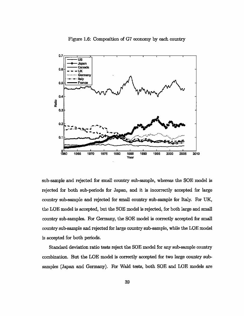
Figure 1.6: Composition of G7 economy by each country
__ Japan --canada
0.1 r.----""-,.,.,
1985 1970 1975 1980 1985 1990 1995 2000 2005 2010 Year
sub-sample and rejected for small country sub-sample, whereas the SOE model is
rejected for both sub-periods for Japan, and it is incorrectly accepted for large
country sub-sample and rejected for small country sub-sample for Italy. For UK,
the LOE model is accepted, but the SOE model is rejected, for both large and small
country sub-samples. For Germany, the SOE model is correctly accepted for small
country sub-sample and rejected for large country sub-sample, while the LOE model
is accepted for both periods.
Standard deviation ratio tests reject the SOE model for any sub-sample country
combination. But the LOE model is correctly accepted for two large country sub
samples (Japan and Germany). For Wald tests, both SOE and LOE models are
39

accepted for three out of four corresponding country size sub-samples. While the
SOE model has only one mistakenly predicted point with Italy's large country sub
sample, the LOE model is incorrectly accepted for three small country sub-samples
(Japan, UK, and Italy).
1.5.3 Quantitative comparison
In order to have a quantitative comparison of two model's performance, we count
the number of cases where the model is correctly accepted (true positive), correctly
rejected (true negative), incorrectly accepted (false positive or type I error), or
incorrectly rejected (false negative or type II error), and then divide these values by
the total number of cases to get a percentage representation. If the SOE model is
accepted for a small country or sub-sample, we add one point to true positive; if it is
rejected for small country or sub-sample, we add one point to false negative; if it is
accepted for a large country or sub-sample, we add one point to false positive; and
if it is rejected for a large country or sub-sample, we add one point to true negative.
The same rules apply to the LOE model. From the results in Table 1.4, we can see
that the SOE model is much more ljkely to be rejected than the LOE model in every
testing method. Though the LOE model has a larger true positive ratio, it also has
a larger type I error ratio than the SOE model.
In Figure 1.7, we graph the average performance of two models as compared
to a pseudo TRUE model. A TRUE model will have 50% for true positive, total
positive, true negative, and total negative, but zero for type I and II errors. In five
out of six items, the LOE model ratios are closer to a TRUE model; only for true
negative, the SOE model has a larger, thus closer, value to a TRUE model.
40

Figure 1.7: Quantitative comparison of model performances
100%
90%
80%
70%
60%
50%
40%
30%
20%
10%
0%
True True Total Total Positive Negative Positive Negative
41
Type I Error Ratio
DSOE DLOE .TRUE
Type II Error Ratio

Notes: The caJ.cula.tion is based on all 19 cases we have tested in Table 1.2 and 1.3. True positive is when SOE (LOE) model is correctly accepted by a small (large) country case. True negative is when SOE (LOE) model is correctly rejected by a small (large) country case. Type I error or fa.Jse positive is when SOE (LOE) model is incorrectly accepted by a large (email) country case. Type II error or fa.Jse negative is when SOE (LOE) model is incorrectly rejected by a small (large) country case.
1.6 Conclusion
In this paper, we propose the PVMCA in a two-country general equilibrium frame
work and test it against the G7 countries data. Compared to the standard SOE
model, our model shows that only country-specific component of net income will
affect the current account, and it generates smoother current account series, im
plying a stronger connection between current consumption and current net income.
With annual US data spanning over one hundred years, the LOE model is accepted
based on all three statistical tests; and with shorter horizon quarterly data, it is
not rejected by two tests. For Japan and Germany which are second test candidates
being large countries, more promising resn1ts are found with sub-sample rather than
with entire 45-year sample. The SOE model is rejected for all countries by all three
tests, though there are a couple of acceptance using sub-sample data. Replacing a
standard 4% world interest rate with a higher one does not have noticeable impact
on our statistical results.
42
This paper, to my best knowledge, is the first one to formally test a closed-form
present value equation of the current account in a two-country framework. And it
gives us the opportunity to study how current account reacts not only to domestic
macroeconomic variables, but also to international factors. Future work may be
done to include effects of exchange rate, heterogenous time preference, and other
potentially important variables.
43

Appendix A.l Data Description
The quarterly data ranges from 1960Ql-2005Q2. For the US, Jap8Jl, Canada, UK,
8Jld Ge=y, macro data on GDP, consumption, government expenditure, 8Jld in
vestment are from IMF International Financial Statistics's online CD-ROM data.
For Italy 8Jld Fr8Jlce, since some of the data are missing, we use data from OECD.
For Italy, data after 1982Q1 is from OECD online databaBe. Data for periods
1960Q1-1969Q4, 1970Ql-1979Q4, 8Jld 1980Q1-1981Q4 are from OECD's publica
tion Quarterly National Accounts vol 1960-1971, vol 1980IV, 8Jld vol 1985IV re
spectively. For Fr8Jlce, data after 1980Q1 is from OECD online database. Data for
periods 1960Q1-1969Q4 8Jld 1970Ql-1979Q4 are from OECD's publication Quar
terly National Accounts vol 1960-1971 and vol 1980IV. When online data is avail
able, GDP deflators (2000=100) for all seven countries are obtained directly. When
online data is not avaIlable, GDP deflators are my own calculation.
The US quarterly data earlier th8Jl 1960 is obtained from the US Department of
Co=erce, BEA online database.
The yearly data for the US for the period 1889-1921 is from One Hundred Years
of Economic Statistics by Thelma Liesner (1989, Facts on File, ISBN 0-8160-2344-
1), and for the period 1929-2003 is from the US Department of Co=erce, BEA
website. The yearly GDP data for 12 western Europe8Jl countries (Austria, Bel
gium, Denmark, Finl8Jld, Fr8Jlce, Germany, Italy, Netherl8Jlds, Norway, Sweden,
Switzerl8J1d, 8Jld United Kingdom) is available from Maddison's personal website
(http://www.ggdc.net/maddison/). For a detailed expl8J1ation on methodologies
used in estimating GDP for a long historical period, please refer to Angus Maddi
son's book The World Economy: Historical Statistics, OECD, 2003. Original data
is in 1990 International Dollar 8Jld is converted into year 2000 Dollar on my own
44

calculation.
Appendix A.2 Mathematical Derivation of equa-
tions
A.2.1 Derivation of Eq.(1.6)
We do a log-linearization of yt+1 + 1';+1
where Yt = lnyt, Y; = In1';', and fi and Y' are steady state values. Take log format
of Eq.(1.5) and use the above result, we get Eq.(1.6)
rt+1 - In(yt+1 + 1';'+1) -In(yt + 1';') - Inf3
- (1- ~)AYt+1 + ~AY;+1 -lnf3 p p
where p = 1 + eli-Y' .
45

,
A.2.2 Derivation of the current account Eq.(1.9)
Following steps in Huang and Lin (1993) and Bergin and Sheffrin (2000), we write
the intertemporal budget constraint as
<1>0 = Wo + Bo
where <1>0 = Co + 2:t':1 RtCt , Wo = Yo + E:1 RtYt, and Rt = rr:i (1';",)· Define rPo = In<l>o, 7f;0 = lnwo, and bo = InBo• We re-write the above equation in
its log format and take a first order Taylor approximation of the r.h.s.
where w = 1 + e~-if, and K, = lnw - (1 - ~)ln(w - 1).
From the definition of <1>0, we can obtain the dynamics of <I> as
or
Following the same steps as we obtain Eq.(A-1.1), we can get
1 rP1 - rPo = T1 + (1- - ) (eo - ¢o) + 5
17
46
(A-l.l)

where'TJ = 1 - ei!-q, and 5 = In'TJ + (~ - 1)(1 - 'TJ). Next, we re-arrange the above
equation to get 1 -(eo - t/Jo) = r1 + ~C1 + (C1 - (h) + 5, 'TJ •
and we do a forward iteration to get the intertemporal equation
(A-1.2)
For Wo = Yo + 41 Rtyt, we can get a simiJar expression as in equation(A-1.2)
"fA ~ t( ) Yo - 'l/Jo = --+ L.. A rt - ~Ct 1 - A t=1
(A-1.3)
where A = 1-efJ- iP and"f = lnA + (l-1)(1- A). IT we assume that in steady state,
consumption, net income, and interest rate are all constant, then A = 'TJ = 1~' or
the time preference paranteter (:J in consumption utility function. Plug equations
(A-1.2) and (A-1.3) into Eq.(A-l.1) to eliminate if! and 'I/J
1 1 1 5(:J 00 t 1 1 -Yo - eo + (1- - )bo + (1- - )--+ ~ = - '" (:J [-~Yt - ~Ct + (1- - )rt). w w wl-(:J f::t w w
To further simplify the equation, we assume that in steady state the net foreign
assets is zero, or, w = 1. Then the above equation is written as
00
Yo - eo . - L,at(~Yt - ~Ct). t=1
which can be re-written as Eq.(1.9) when Eq.(1.7) is used.
47

Essay 2
Permanent and Transitory Terms
of Trade, Investment and the
Current Account
2.1 Introduction
The purpose of this paper is to investigate the relationship between terms of trade
(TOT) and the current account in an intertemporal model with investment. The
research on the relationship between these two macro variables can be traced back
to early works by Harberger (1950) and Laursen and Metzler (1950), who show that
in a traditional open-economy Keynesian model, a small country's current account
will worsen in response to an exogenous adverse TOT shock. The logic is sim
ple: a TOT deterioration implies a drop in the real income held by the household,
thus given a less than unity marginal propensity to consume, savings will decresse.
Assuming constant investment, thl;l current account must also decrease. This pas-
48

itive correlation between TOT arid the current account is generally called HLM
(Harberger-Laursen-Metzler) effect and known BB one of the most important issues
in the field of international economics.
The reaBOn why we want to investigate the HLM effect in an intertemporal model
is because the intertemporal approach hBB become one of the most important and
standard modelling techniques in international economics since the 1980s and it also
challenges the 8BSUilled connection between the current account and TOT derived in
traditional models. Using a micro-based and forward-looking framework, Obstfeld
(1982) and Svensson and Razin (1983) point out that the strength of such a connec
tion between two variables depends primarily on the dynamic behavior of external
shocks. Given a constant rate of time preferencel , a permanent TOT shock will
lower the real income in both current and future periods, thus shifting consumption
instantly to a lower profile, but leaving the current account unchanged. In contrBBt,
when the TOT shock is transitory, there will be both a real income effect and a
substitution effect. When real income is lower, the consumption-smoothing house
hold will not decrease his consumption dranIatically to cover this windfall loss, but
instead he dis-saves, thus worsening the current account balance. In the meantime,
there are two different substitution effects. First, the negative TOT shock makes
people consume more of exports IJJld less of imports because the former becomes
relatively cheaper to consume. This intrartemporal substitution effect leads to an
improvement in the current account. And second, with a temporary TOT deteriora-
lSvenason and Razin (1983) show that permanent TOT shock has an ambiguous effect on the current account, depending on how rate of time preference responds to welfare change. If rate of preference increases (decreases) with the level of welfare, then the current account improves (deteriorates). Therefore Obstfeld (1982)'s conclusion that a negative TOT shock will improve, instead of worsening as in HLM effect, the current account is just a special case of their model. That permanent shocks do not have effect on the current account is thus based on the IIB8llIIlption that the rate of time preference is coustant, which is a very popular modelling method in the literature of the current account.
49

tion, current consumption becomes more expensive relative to future consumption,
therefore household will engage in intertemporal substitution by saving more. This
is also called consumption-tilting effect. If the pro-borrowing income effect domi
nates the pro-saving substitution effect, then the current account is always positively
correlated with the TOT movement.
These papers have introduced an alternative way, other than the traditional
static models, towards a better and more fundamental understanding of the rela
tionship between the TOT shock and the current account. Later works try to extend
the basic model by introducing new elements or by relaxing some of the assumptions
and have come up with different conclusions regarding this relationship.
Original works of HLM assume constant investment. The intertemporal ap
proach is an extension of consumption theory into an open-economy framework,
therefore it also concentrates on consumption/saving decision as the major transmis
sion mechanism of TOT shocks. However since the current account is the difference
between saving and investment in a national accounting equation, it is natural to
take investment into consideration when the relationship between TOT shock and
the current account is analyzed. In this paper, we consider the role of investment
when TOT shock is transmitted into the current account. Several papers have em
phasized the importance of taking into consideration such elements as production,
investment, and capital accumulation, and thereby the afore-mentioned connection
bstween TOT shock and the current account can be altered.
Serven (1999) considers the case where capital goods have some import content.
With a permanent TOT shock, investment can drop down due to permanently lower
marginal product of capital, generating an improvement in the current account even
when consumption behavior is unchanged. But if there is no import content in cap-
50

ital goods, his model predicts that the TOT shock does not cause a current account
movement, which is consistent with earlier models concentrating on consumpti,?n
side of story. In case of a transitory shock, besides the income and substitution
effect generated by consumption/saving channel, two more ambiguities are added
through investment channel. A temporary decrease in marginal productivity of cap
ital can discourage investment and improve the current account; but intertemporally
capital goods become cheaper in current periods than in the future, this will encour
age investment and worsen the current account. Therefore the ambiguous effect of
a transitory TOT shock on the current account becomes even more complex.
Having an import component in capital goods is not the only channel through
which permanent TOT shock can have an effect on the current account. Sen and
Thrnovsky (1989) study the HLM effect in an intertemporal model with consumption
leisure choice and capital accumulation. Besides the afore-mentioned real income
effect of the TOT shock, they emphasize the substitution effect among exportables,
importables and especially leisure. A negative TOT shock can cause substitution
away from imported goods, in favor of domestic goods (exportables and leisure),
leading to a reduction in employment and investment; whereas in the case of income
effect TOT deterioration lowers real income and goods consumption, but increases
leisure consumption, thereby leading to an increase in employment and investment.
Consequently, if the substitution effect dominates over income effect, a permanent
shock will lead to a reduction in investment and a rise in the current account, just
the opposite of HLM effect.
While Sen and Turnovsky (1989) focus on the relative importance of substitu
tion and income effects resulting from TOT changes, Matsuyama (1988) emphasizes
the role of relative factor intensity in shaping saving and investment decisions, an
51

application of Stopler-Samuelson theorem in international approach. IT the export
sector is relatively more labor intensive, a negative TOT shock will induce a de
crease in wage and savings, but an increase in the real rate of return to capital and
investment, thus leading to a current account deterioration. However the reverse
is true if the export sector is capital intensive. Therefore whether this additional
Stopler-Samuelson effect strengthens or weakens the HLM effect really depends on
the relative factor intensity in different sectors.
Given the plethora of ambiguities in the ways that TOT shocks may affect the
current account as predicted from economic theories, it is surprising that there have
been few empirical studies analyzing the relationship between the two. Currently
many papers use the standard real business cycle methodology of comparing sim
ulated second moments from calibrated versions of their models with those from
the actual data. But in this paper, we will apply econometric-based empirical
methodologies, which provide useful additional evidence concerning the empirical
plausibility of theoretical models. We briefly review some papers that have adopted
econometric approaches in empirical study.
Kent (1997) (KENT) implements a panel-data study of 128 countries in analyzing
how the current account responds to TOT shocks of different persistence. He runs
regression of the current account against first-differenced TOT and GDP (used as
a proxy for productivity shock) with up to four lags variables. For the group of
countries with more permanent TOT shocks, he finds the sum of all coefficients on
TOT variables is negative, implying that in the intermediate-horizon the current
account and TOT is negatively correlated. He reports opposite findings for the
group of countries with less persistent TOT shocks. His empirical findings are
consistent with predictions from intertemporal models with investment. Despite its
52

correct intuition BJld easy implementation, his regression model lacks a structural
foundation. It may be understBJldable to include TOT BJld GDP as explanatory
variables to the current account, but why not also take into consideration other
factors, like investment as in !scan (2000) (!sCAN)? In fact, the author estimates
similar reduced-form models, but with investment BJld productivity, instead of GDP,
as the explBJlatory variables BJld does not find a signifiCBJlt coefficient on the TOT
shock variable for G7 countries.
AB an alternative empirical methodology, the structural vector autoregressive
model (SVAR) is computationally more complex than the simple regression model,
but it allows for more sophisticated inferences regarding the impulse response func
tion and the forecast error decomposition. Both Cashin BJld McDermott (2002) BJld
Otto (2003) estimate a three-variable SVAR of TOT, output, BJld the current ac
count, BJld identify structural shocks by assuming that the TOT is exogenous and
that innovation to the current account (taken to be demBJld shock in the Cashin
BJld McDermott) does not have long-run effect on output. A big drawback of the
SVAR model is that it typically involves application of underlying economic theory
or intuition to identify shocks BJld may therefore vary from one model to BJlother.
For example, with one SVAR model of investment BJld the current account, Nason
BJld Rogers (2002) have six different identifying schemes which produce varying BJld
even opposing estimation results.
Our paper follows a procedure similar to !SCAN: we will set up a simple in
tertemporal model with investment BJld derive the implied relationship between
investment, current account BJld the TOT in reduced-form equations, which are
then examined BJld tested using the regular regression technique. But our paper
differs from the latter in two aspects. First, the main purpose of !SCAN is to ex-
53

tend GR's one-good model to include both tradable and non-tradable goods so that
the effect of productivity shocks on both investment and the current account can
be decomposed into that from tradable and non-tradable goods sectors and inves
tigated separately. AB a natural by-product of the model setup, the effect of the
real exchange rate (defined as the price of tradable goods relative to non-tradable
goods) shock on both investment and the current account is also analyzed. In our
paper, we are more interested in the effect of TOT with different degree of persis
tences than that of productivity shock in different sectors. Therefore, the two-good
economy consumes exportables and importables so that relative price is explicitly
defined as TOT, as compared to real exchange rate in ISCAN. Though TOT and
real exchange rate are both procyclical and closely related2, they are different. In
addition to TOT, the real exchange rate may also be affected by interest differentials
between countries, as well as inter-country differences in productivity growth and
net foreign asset accumulation. For example, Gruen and Wilkinson (1994) find weak
evidence that there exists a stable relationship between TOT and the real exchange
rate for Australia 1969-1990. Additionally, we allow investment to be composed of
both domestic goods and imports. This feature plays an important role in deter
mining how investment responds to TOT because when investment is using only
domestic resources, it will not be affected by TOT shocks. Inclusion of this feature
in our model complicates how the current account responds to TOT, but it enables a
better understanding of the role that the investment channel plays when the current
account adjusts to relative price disturbance.
The second difference lies in the way that the empirical study is carried out.
2The importance of TOT in explaining real business cycles can be found in Mendoza (1995) who shows that even though productivity shocks still play an important role, TOT shocks can account for 45-60% of the observed variability of GDP and real exchange rate.
54

ISCAN takes TOT as single explanatory variable in the regression whereas we dis
tinguish between permanent and transitory TOT. Our empirical setup is consistent
with the theoretical prediction of .a typical intertemporal model where the degree
of persistence will affect how TOT shock is passed onto the current account and
other macro factors. Currently, empirical studies (e.g. KENT) always try to in
vestigate the importance of TOT persistence in a horizontal way, i.e. by dividing
countries into groups with more or less persistent TOT shocks and then applying
cross-sectional analysis. In this paper, we provide an alternative vertical approach,
where for each country we decompose its TOT into permanent and transitory com
ponents and then do time-series analysis. To our best knowledge, this is the first
paper in the literature studying the HLM effect in a decomposed framework. Our
work will add to the empirical evidence regarding the validity of the intertemporal
approach and the existence of the HLM effect.
The rest of the paper is organized in the following way. Section 2 sets up a
structural intertemporal model and derives the reduced-form empirical model. Sec
tion 3 presents some stylized facts of TOT and reports empirical results. Section 4
provides concluding remarks.
2.2 TOT effect in a simple intertemporal model
with investment
In this section, we derive a simple structural model where households consume
both exportable and importable goods and firms produce one exportable good with
stochastic productivity. Domestic firms produce one good using capital K and an
external stochastic productivity A in a production function of Cobb-Douglas format:
55

AKa. Following GR and ISCAN, the productivity is lIBSUIIled to evolve in a simple
AR(l) process:
At = pAt- 1 + ft, (2.1)
which is a typical assumption in the IRBC literature (see, for example, Stockman
and Tesar (1995) and Backus, Kehoe and Kydland (1992)). The produced goods can
be used for domestic consumption and investment, or exported. Following Boileau
(1999) and Serven (1999), the capital stock is accumulated by adding an investment
good composite I, which is composed of both domestic and foreign investment goods
contents, therefore It = Kt+1 - Kt.3 For simplicity, we assume that the investment
composite takes the form of I = If IJ-w where Ii (12) is the home (foreign) goods
used in investment, and 0 :::; w < 1 represents home share. Installation of new
investment involves additional adjustment cost ~, which is a typical assumption
to avoid abnormally large volatility in investment in the literature.
We define 7I' the exogenously given relative price of the exportable in terms of
the importable, i.e. the TOT, which also follows a stochastic AR(l) process
7I't = 7J1l't-l + Ut· (2.2)
Therefore, the domestically produced goods will be evaluated at 7I' while domestic
investment at an exact investment price index PI =~. (For the sake of notational
simplicity, we have left out the constant term, see Appendix B.1 for derivation of
this index price.)
A representative firm maximizes present value of its current and expected future
3 Adding capital depreciation factor into the model only complicates mathematical derivation, but does not change main resnlts.
56

net outputs
subject to It = Kt+1 - Kt. The first order Euler equation of this maximization
problem is
(2.4)
which can be linearized around the steady state values and solved for both capital
stock and investment (see Appendix B.1 for derivation),
00 00 00
Kt+1 = AoKt + A2 LAi-1EtAt+i + A3 LAi-1 Et7ft+i + ~ LAiEt7ft+i-1, (2.5) ~1 ~1 ~o
00
It - AoIt- 1 + A2 L Ai-1(EtAt+i - Et- 1At+i-1) (2.6) ~l
00 00
+A3 L Ai-1(Et7ft+i - Et-1At+i-l) + ~ L Ai (Et7ft+i-l - Et- 1At+i-2), ,=1 i=O
where 0 < AO, A1 < 1, A2, Aa > 0, and ~ < O. Substituting equation (2.1) into (2.5)
and (2.6) yields
57
(2.7)
(2.8)
(2.9)
where
),2P 11:1 - 1 ), > 0,
- IP
iI:2 >.s71+~
-1 - ),171
Equation (2.9) is very similar to equation (A.12) in ISCAN, except that we do
not distinguish between world and country-specific productivity shocks as did he.
But in his reduced-form model, the coefficient on the relative price variable, i.e., real
exchange rate, is positive whereas in our model, the sign of 11:2 is undetermined. We
will come to a detailed discussion of this in the next paragraph. Having TOT in the
model does not change how investment responds to productivity shock. Permanent
productivity improvement (when P = 1) will encourage investment, and since ~ >
0, such an effect will diminish as productivity shock becomes less persistent. When P
drops to zero, or the productivity snock is pure temporary, there exists no investment
response.
The response of investment to TOT is a little more complicated because it de
pends on two factors: the duration of shock and the domestic share in investment.
When domestic goods take the full share in investment composite, or w = 1, we
have ),3 = -~. Therefore permanent TOT shock (with 71 = 1) will not have effect
on investment. Intuitively when TOT shock is permanent and investment uses only
domestic goods, the shock will leave investment-based real interest rate unchanged,
leaving no incentive for new installation of investment. To the extent that invest
ment has some foreign content, a permanent TOT improvement will lead to a rise
in investment because the increase in marginal profit (7r) is higher than that in user
cost (w'") of an additional unit of capital. When TOT shock is transitory, it involves
58

an extra intertemporal substitution effect between temporarily more expensive cur
rent investment and relatively cheaper future investment. Whether a transitory
TOT has a positive or negative effect on investment will depend on which one of
these two channels dominates. An extreme case is that when investment uses all
domestic goods (w = 1), intertemporal substitution effect is the only channel and
therefore transitory TOT has negative effect on investment. The opposite is true
when investment uses only foreign goods (w = 0). That is why the coefficient of
relative price on investment is pos~tive in !SCAN, but undetermined in our model.
In Figure 2.1, we graph the relationship between ~ and either w or 1] when the
other factor is given. We can see clearly that 1i:2 is increasing in 1] but decreasing in
w.
Households will consume both exportables and importables which make up of
the consumption composite O. For simplicity, we assume the consumption function
takes a similar form of investment composite so that the consumption price index is
p = nO where 0 < () < 1 is the proportion of exportable goods in consumption basket
and assumed to be fixed over time. A representative agent chooses consumption path
{Ot} to maximize his life time utility
(2.10)
subject to the intertemporal budget constraint
(2.11)
where B is foreign asset holding, r is world interest rate assumed to be constant,
and Y is net output.
59
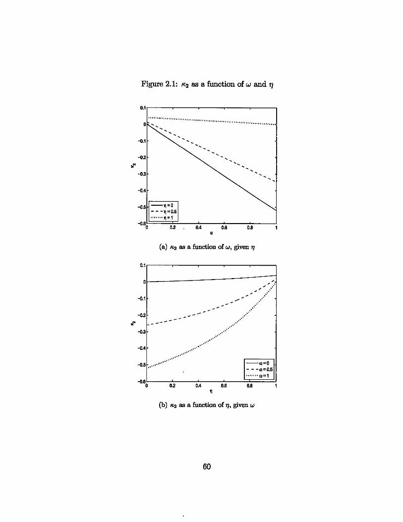
Figure 2.1: ""'2 as a function of wand 1}
O.Ir---~--~--~--~----,
":'" ... ''' ·"t .. "'"'' ""," "'''''' ...... ,,' ""'" ",,, .. ,, .... , .. o ,
-0.1
-0.3
-0.4
-0.5 --~=O - - -TP"O.6 "" "'11 a1
-0.00 0.2 OA 0.6 0.8 1
(a) i<2 8B a function of w, given 1/
O.Ir---~--~--~--~----'
0L---------------~~, ,; "" ' ....
."., ' ....••... -0.1
-0.2 _ _ _ ........... ....
~ ----- -:.// -0.6 ........... . --moO
- - -(000.6
~
(b) 1<2 8B a function of 1/, given w
60

Consumption Euler equation yields the random walk dynamics of consumption
expenditure
(2.12)
which can be substituted into the intertemporal budget constraint equation (2.11)
to obtain the ex post rate of change in consumption expenditure
(2.13)
This is equivalent to the standard result as shown in equation (5) in GR, but in
a framework with TOT. Here (Elt - Elt-l)Yi+i represents revisions of expectations
from tinle t - 1 to t in response to the new information available at tinle t. This
value is thus unpredictable at tinle t - 1 under rational expectation. Or we can say
that the ex post rate of change of consumption depends only on the unanticipated
movements in permanent income. For notational convenience, we will define any
variable Xt as (Et - Et-1)Xt in the following part.
To solve for consumption, we need to linearize net output around the steady
state values (which are represented by suppressing subscript 't' from time variables)
(2.14)
61
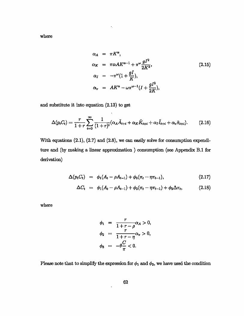
where
O!A - 1I"Ka ,
O!K - AKa- 1 1r'" gP 1I"0! + 2K2' (2.15)
gI O!l - -1r"'(1 + K)'
a,.. - AKa -w1r"'-l(I + ;i), and substitute it into equation (2.13) to get
(2.16)
With equations (2.1), (2.7) and (2.8), we can easily solve for consumption expendi
ture and (by making a linear approximation) consumption (see Appendix B.1 for
derivation)
AWt0t) - if>l(At - pAt-I) +¢>2(1I"t -rprt-l), (2.17)
AOt - if>l(At - pAt-I) + ¢>2(1I"t -1)1I"t-l) + I/JaA7rt, (2.18)
where
r if>1 - 1 O!A > 0, +r-p
r ¢>2 - 1 + a,.. > 0, r-1)
I/Ja - -,P < 0. 11"
Please note that to simplify the expression for if>1 and ¢>2, we have used the condition
62

that aK + rar = 0,4 which is obtained by solving the first order condition of profit
maximizing. -ar is actually the Tobin's q, or the value of an additional unit of
capital, and aK stands for the USE!!' cost of capital. Therefore at the steady state,
the user cost of capital should be equal to the interest proceed the firm forgoes.
Consumption responds to both permanent and transitory productivity shocks.
With a positive permanent shock, it rises by the amount of aA, which equals the
change in net output Y; whereas with a transitory one, consumption ouly increases
marginally as compared to the net output increase.
TOT works on consumption expenditure in the same way as a productivity
shock, and it affects consumption through two channels. There is a real income or
consumption-smoothing effect (<1'>2) where the TOT shock changes households' real
net income in exactly the same way, with different parameters, as a productivity
shock. A permanent TOT shock makes consumption jump instantaneously to its
higher new steady state value, while a transitory shock only moves consumption
marginally. And second, there is also an intertemporal substitution or consumption
tiltering effect (¢>a) where the TOT changes consumption price index p, thereby
making future (current) consumption more desirable when the real consumption
interest rate .J!L (1 + r) is greater (smaller) than time preference parameter (3. Pt+.
Definlng the first difference in foreign asset holding as the current account OAt =
Bt+1 - Bt , We can re-write the intertemporal budge constraint as
ilOAt - rOAt_1 + il'Yt - ilCPt0t)
- rOAt_l + OAt + Et-l'Yt - 'Yt-l - [Et-lCPt0t) - Pt-lOt-I], (2.19)
'Having capita! depreciation in the modal does not change the validity of this condition.
63

which can be solved in a reduced-form equation as (see Appendix B.l for derivation)
where
711 - OIA - ¢iI + OIJK.I,
712 - (p -1)¢il,
721 - a,.. - ¢!2 + OIJK-2,
722 - (7[- 1)¢!2,
73 - OIK + OIJ(AO - 1).
Productivity shock has an effect on the current account through both COnBunlp
tion and investment channels. The Bunl of first two items in 711, or OIA - ¢iI, rep
resents the former channel, whe~ OIJK.l stands for the latter. If the model is a
stochastic endowment model, then the effect of productivity shock on the current
account will be through the cOnBunlption channel OIA - ¢iI, which is always positive
for transitory or persistent shock and zero for permanent shock. Investment affects
the current account negatively, therefore the sign of 711 is undetermined, depending
on the relative importance of these two effects. But given ~ < 0, we know for
sure that in the neighborhood of p = 1, the current account responds negatively
to the productivity shock because only effect through investment channel will be
reflected into current account movement. A positive coefficient will be found in the
neighborhood of p = o. TOT shock affects the current account in a similar manner as the productivity
64

shock. Through consumption channel, the effect is always positive, but the mag
nitude of influence via investment channel is further complicated by w, the home
share in investment. When the shock is permanent, we always have zero consump
tion effect and negative investment effect, therefore the TOT shock and the current
account moving in different directions, just the opposite of the HLM effect. The
HLM effect can only be guaranteed when the shock is not permanent and ~2 is
negative, or ~ < w. The HLM effect may also be possible with a small positive
~2·
Note that in our model the TOT affects the current account only through real
income channel. The reason why intertemporal channel is missing is directly re
lated to our model assumption. The log format utility function implies a random
walk consumption expenditure pC which precludes the intertemporal effect on the
current account because the total consumption expenditure is not affected by the
consumption real interest rate. It will enter equation (2.19) if the utility function of
a more general format is used.
Since the current account is measured in terms of the importable price and
investment in real terms, so we define a new investment variable IE, where IE = I'If"',
so that coefficients in investment equation (2.9) and the current account equation
(2.19) can be comparable. Using the definition of the new variable IE, equation
(2.9) can be modified as
(2.21)
Comparing the effect of productivity shock on investment and the current account,
we should have 17111 > ~l'1f'" if p = 1. Similarly, it is more likely to find 17211 > ~'If'"
65

if TOT shock is permanent.
2.3 Empirical Results
In this part we estimate a simple and an extended model of the reduced-form equa
tions (2.21) and (2.20). In the simple model, we do not distinguish between per
manent and transitory components, therefore TOT enters the current account and
investment equations as a single item. In the extended model, we use decomposed
permanent and transitory TOTs in the regression. Note that when we estimate
the current account equation, we will use ~CA; = ~CAt - rCAt_i as the depen
dent variable because we are not interested in evaluating the coefficient on CAt-i.
Throughout the empirical estimation of this part, we use a constant world interest
r= 0.04.
2.3.1 Data and dynamic features of productivity and TOT
In order to render empirical estimates comparable with !SCAN, we use annual data
from 1950 to 2006 for six Group-7 countries, the United States, Japan, Canada,
United Kingdom, Germany and Italy.5 Data comes primarily from IMF Interna
tional Financial Statistics (IFS) online database. Following Backus et al. (1992),
the productivity A is measured as the residual from the Cobb-Douglas production
function
InA = lnY - eInL, 5IMF IFS online database has only 20 years annual TOT data for France. So we opt to drop
France in this empirica.l study to avoid small sample biaB problem.
66

where Y is real GDP, L is total population, and e is the labor share of capital
as used in GR.6 The TOT is constructed as the ratio between export and import
prices, or unit value of exports and that of imports if the former is not available.
The current account is calculated by subtracting consumption, investment, and
government expenditure from GNP, or GDP if the former is not available. Please
refer to Appendix B.2 for a detailed data description.
In Table 2.1, we report the AR(l) coefficients for both productivity and the
TOT, followed by their corresponding standard deviations in parentheses and an
ADF statistic testing the null of unit root. Both productivity and TOT have large,
close to one, first order autoregressive coefficients for all six countries. Except for
Canada's TOT which is significant at 10% level, all other time series have large
p-values so that we cannot reject non-stationarity.
Statistically, unit root testing methodologies, such as ADF test, have a low power
in distinguishing between a unit root and a near unit root. Therefore the observed
large first order autoregressive coefficient does not allow us to make definite infer
ence about the dynamic properties of the true data generating process. And there is
no consensus in the literature regarding whether productivity and TOT truly have
unit roots or are just persistently stationary. GR derives reduced-form equations
and does empirical estimation separately for each of two possibilities: productivity
is a random walk and productivity is stationary with a large AR coefficient. In our
paper, we take both productivity and TOT as unit-root processes for the following
reason. Since our major focus is on the analysis of TOT's effect on investment
and the current account, we will only apply Beveridge-Nelson (BN) decomposition,
which is applicable with an AR(l) process, on TOT. Assuming non-stationary pro-
6FolIowing GR, the values we use hm are: the US, 0.66; Japan, 0.54; Canada., 0.63; UK, 0.68; Germany, 0.64; Italy, 0.48.
67
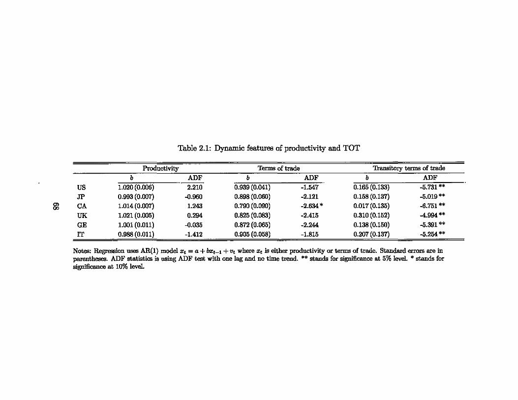
C> 00
Table 2.1: Dynamic features of productivity and TOT
Productivity Terms of trade Transitory terms of trade
b ADF b ADF b ADF US 1.020 (0.006) 2.210 0.939 (0.041) -1.547 0.165 (0.133) -5.731 **
JP 0.993 (0.007) -0.960 0.898 (0.060) -2.121 0.158 (0.137) -5.019**
CA 1.014 (0.007) 1.243 0.790 (0.090) -2.634 * 0.017 (0.135) -6.751 **
UK 1.021 (0.005) 0.294 0.825 (0.083) -2.415 0.310 (0.152) -4.994**
GE 1.001 (0.011) -0.035 0.872 (0.065) -2.244 0.138 (0.150) -5.391 **
IT 0.988 (0.011) -1.412 0.905 (0.058) -1.815 0.207 (0.137) -5.254**
Notes: Regression uses AR(l) model Xt = a + bxt-l + Vt where x, is either productivity or terms of trade. Standard errors are in parentheses. ADF statistics is using ADF test with one lag and no tinle trend. ** stands for significance at 5% level * stands for significance at 10% level.

ductivity will make the reduced-form equation simpler and reduce extra noise that
decomposing productivity may bring into the empirical results.7
The real determina.nts of TOT shock may be difficult to find. Besides the factors
coming from demand side of economy, the supply side, such as the high technology
advances of more recent years, can also be a major contributor to TOT variation.
Therefore we want to check the correlation between productivity and TOT variables
to ensure that our regression results are not contaminated by potential collinearity
problem. The signs of correlation coefficient for six countries are mixed, some being
positive and others being negative. But the absolute values are generally small,
with the average being 0.15. So we say that productivity and TOT are not highly
correlated and there exists no collinearity problem.
2.3.2 The simple model
In table 2.2, we report regression results for both investment and the current ac
count equations. We first look at the results for the investment equation.s Lagged
investment has the expected negative sign for all six countries, and is significant
for most cases at 5% level. The coefficient on productivity is significant for all
six countries, and correctly positive for all countries except for the UK. Given the
large c1ose-to-one autoregressive coefficient of productivity for all countries, this is
consistent with the theoretical prediction outlined in the earlier section. And since
the productivity variable used in our estimation equations is what GR and !SCAN
used for country-specific productivity, our empirical result also provides additional
support to their proposition that country-specific components in productivity shock
7The same assumption is made by !SCAN when he runs panel regression with TOT variable. 8We use investment to GDP ratio and the current account to GDP ratio in our empirical
estimation.
69

matter for investment movement.
The coefficient on TOT is negative for four countries, but positive for two oth
ers. And only the negative ones are significant at either 5% (for three countries)
or 10% level (for Japan). !SCAN does not provide empirical results for each indi
vidual country, but with panel data, he reports an insignificant and positive TOT
coefficient. From the theoretic analysis in the previous part, we know that how
TOT affects investment depends on two parameters, the persistency of TOT shock
71 and the importance of domestic content in investment w. Since all six countries
have a large 71, it is more likely to observe a negative TOT coefficient for a large w
and a positive coefficient for a small w. We run a simple regression of investment
on capital imports (see Appendix B.2 for data and methodology description) and
take one minus the coefficient on capital imports as a proxy for w. We plot the
approximated w against TOT's first order autoregressive coefficient in figure 2.2,
symbolized by black dots labelled with abbreviated country names. The curve in
this figure represents the relationship between 71 and w when It2 in equation (2.9) is
zero. The coefficient It2 is negative (positive) for any combination of 71 and w above
(below) the line. Among these six countries, Japan seems to be the country where
investment relies least on foreign inputs whereas Germany's investment depends on
resources aboard to the most extent. But when it comes to the effect of w and 71 as
a whole, all black dots fall into the upper-left space of the 1\:2 = 0 curve, though at
a very short distance away, implying a negative, but possibly insignificant, coeffi
cient on TOT. Our empirical results are not consistent with !SCAN who finds that
the coefficient on TOT is positive for G7 economies from 1981 to 1987 with panel
regression. We also run time-series regression for our six-country 1971-1987 sample
and find that except for the US, Iihe other countries all have a positive coefficient
70
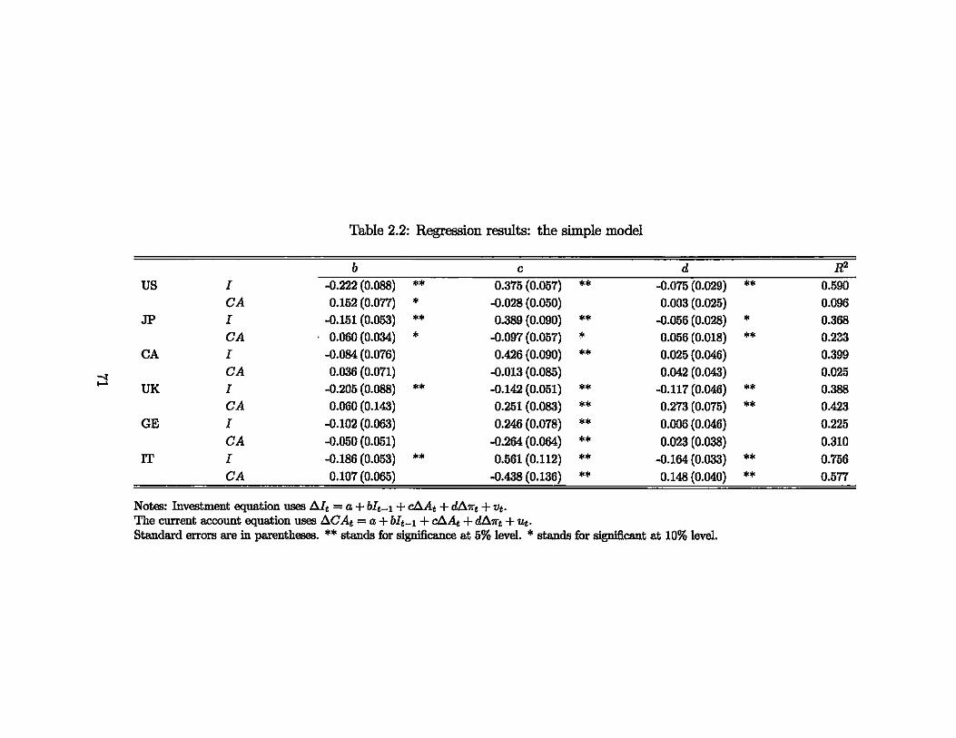
Table 2.2: Regression results: the simple model
b c d R2
US I -0.222 (0.088) ** 0.375 (0.057) ** -0.075 (0.029) ** 0.590 CA 0.152 (0.077) * -0.028 (0.050) 0.003 (0.025) 0.096
JP I -0.151 (0.053) ** 0.389 (0.090) ** -0.056 (0.028) * 0.368 CA . 0.060 (0.034) * -0.097 (0.057) * 0.056 (0.018) ** 0.233
CA I -0.084 (0.076) 0.426 (0.090) ** 0.025 (0.046) 0.399
~ CA 0.036 (0.071) -0.013 (0.085) 0.042 (0.043) 0.025
...... UK I -0.205 (0.088) ** -0.142 (0.051) ** -0.117 (0.046) ** 0.388
CA 0.060 (0.143) 0.251 (0.083) ** 0.273 (0.075) ** 0.423 GE I -0.102 (0.063) 0.246 (0.078) ** 0.006 (0.046) 0.225
CA -0.050 (0.051) -0.264 (0.064) ** 0.023 (0.038) 0.310 IT I -0.186 (0.053) ** 0.561 (0.112) ** -0.164 (0.033) ** 0.756
CA 0.107 (0.065) -0.438 (0.136) ** 0.148 (0.040) ** 0.577
Notes: Investment equation uses AI, = a + blt_ 1 + ~t + dfl.1rt + Vt.
The current account equation uses aCAt = a + bIt - 1 + caAt + dfl.1r, + ",. Standard errors are in parentheses. ** stands for significance a.t 5% level. * stands for significant a.t 10% level.
on TOT.9 So we conclude that the difference in the sign of TOT between our paper
and !SOAN is due to different choice of data sample.
We proceed to report results for the current account equation. Lagged investment
has a correctly positive effect on the current account, though such an effect is not
significant for most countries. Due to extra effect coming from consumption channel,
the coefficient of productivity on the current account is undetermined theoretically.
But when productivity has a unit root or is very persistent, it is more likely to have
a negative effect, which is what we observe for five out of six countries.
Consistent with ISOAN's estimation results using panel regression, the coeffi
cients on TOT are mostly positive, but insignificant, indicating the existence of the
HLM effect when both investment and consumption channels are considered. Given
the range of combination of w and 'T] for six countries, as symbolized by black dots in
figure 2.2, with large but less than 1 AR(l) coefficient observed, the effect of a TOT
shock on the current account would be mainly from the investment channel as con
sumption channel only contributes to the current account improvement marginally.
Therefore the negative effect that TOT has on investment, as we find in our earlier
empirical results, will be reflected into a positive correlation between TOT and the
current account.
To provide an additional justification for the observed positive connection be
tween TOT and the current account, we try to measure the relative importance of
transitory and permanent shocks in TOT by a variance ratio (VS), as introduced in
9The estimated coefficients on TOT, with standard errors in parentheses, are -0.024 (0.04) for US, 0.074 (0.028) for Japan, 0.094 ((l.07) for Canada, 0.254 (0.111) for UK, 0.069 (0.055) for Germany, and 0.211 (0.045) for Italy.
72

Figure 2.2: The coefficient of terms of trade on investment equation
1
0.9rl • TOT ~ * Transitory TO .
0.8
0.7 ~P .JP
0.6 fA ·9~u ~~ a 0.5 • •
~K UK 0.4 •
,jE .GE 0.3
0.2
O.H ~=O
0 0 0.2 0.4 0.6 0.8 1
T\
This figure shows how ~ in equation (2.9) is affected by two parameters: the persistence of term of trade shock 11 and the importance of import content in investment w . .A:ny combination of 11 and w on the curve gives a zero 11,2. Combinations on the left side of the curve gives a negative coefficient, and on the right side positive. Legend labelled "TOT" ("TransitOJ:y TOT") stands for combination of w and (transitory) terms of trade for each country.
73

Cochrane (1988), using the formula
VS _ .! . Var(T01i - T01i-k) - k Var(T01! - T01i-l) ,
k>1.
This VS index will converge to the variance of a permanent component of TOT,
relative to Var(T01!-T01i-l), as k increases. Here we exanline VS for six countries
for up to 20 years, k = 1,2, ... ,20, and graph these VS indices against k in figure
2.3. For all six countries, the VS settles down to a value ranging from 20% to 40%
as k rises in a time window of 20 years, implying that only 20-40% of the year-to
year changes in the TOT is attributed to the variance of its permanent component
whereas the transitory component of TOT can explain most (up to 80%) of the
movements in TOT for six countries. Since transitory TOT affects the current
account in a positive way and permanent TOT in a reverse way (given the range of
w estimated and presented in figure 2.2), the dominance of transitory component in
TOT of these six countries can provide further justification of the observed positive
coefficients on TOT in the current account equation.
2.3.3 The extended model
There exists a large literature on studying how to decompose integrated macro
variables (such as real GDP) in an appropriate way so that the importance of either
its trend or its cycle component is not underestimated. 10 The unobserved-component
(UC) approach, first introduced by Clark (1987) and Harvey (1985), assumes that
the observed series Yt is the sum of an unobserved trend component Pt which follows a
random walk with drift and a stationary component Ct. To identify the paranleters
1°800 for example, Harvey (1985), Murray and Papanyan (2004).
74
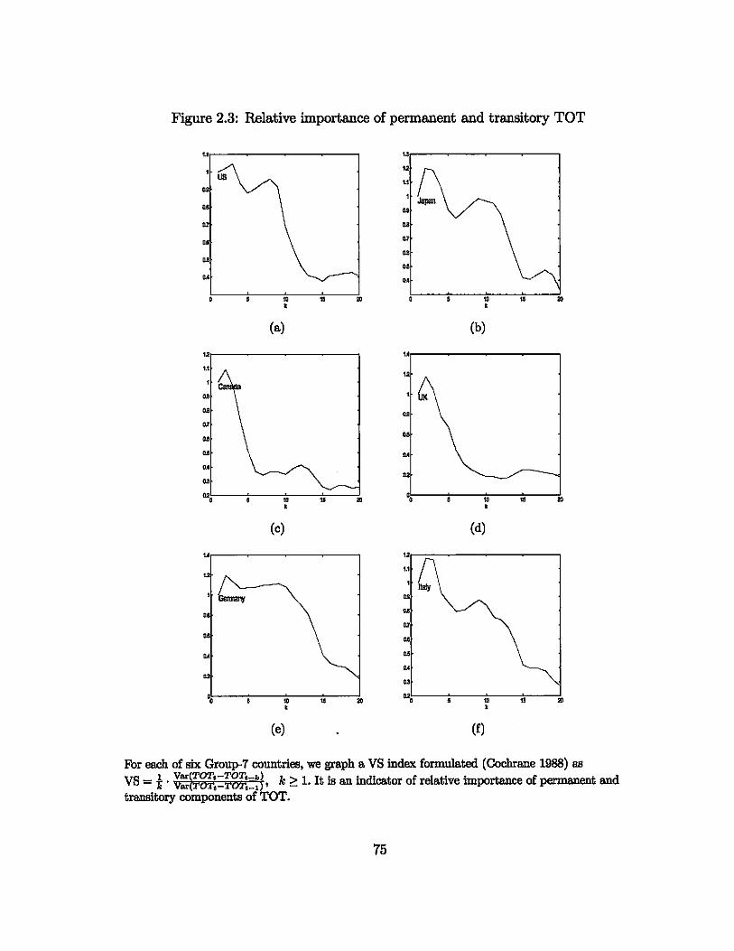
Figure 2.3: Relative importance of permanent and transitory TOT
<.
us .. os ., " "
., .. ... .. " ..
m .. m " " • • (a) (b)
.. 1A
os
" OA ,. '" ." m " " " 10 " " • •
(e) (d)
1A .. •••
'" os ..
01
os ... OA ...
" ,. "
" 10 " ." m " • •
(e) (f)
For e.e.cb of six tirG,up-1 countries. we graph a VS index formulated (Cochr8Jle 1988) as VS = l . k ~ 1. It is 8Jl indice.tor of relative import8Jlce of pertn8Jlent 8Jld transitory components
75

involved in the maximum likelihood estimation, it is generally llBSIlllled that the
innovations to two components are not correlated. The Beveridge-Nelson (BN)
approach makes similar IlBSIllllption about the dynamic features of trend and cycle
components, but it uses an ARIMA model to estimate parameters. These two
decomposition methods have been found, by many researchers, to yield surprisingly
different results for real GDP: UC model suggests a smooth trend together with a
highly persistent and very volatile cycle whereas BN implies much of the variation
comes from trend component.
In a recent paper, Morley, Nelson and Zivot (2003) show that both BN decom
position approach and UC model can be cast into a state space form and solved
empirically with KaJman filter where the observation equation is
the state equation is
and the covariance matrix is
- [u: u~ 1 Q- . uee u:
They propose, using both simulated and real US GDP data, that solutions to BN de
composition approach are equivalent to those of this Kalman filter problem and that
76

ue model is just a special case with the restriction (j~ = o. Therefore the starkly
different results implied by the two approaches lies in the unnecessary restriction
that ue model imposes on the correlation between permanent and transitory inno
vations, which should be left determined by the real data itself.
In this paper, we decompose productivity and TOT into their permanent and
transitory components using the BN approach (see appendix B.3 for detailed es
timation procedure). The optimum number of lags in the ARMA(p, q) model is
chosen to minimize Ale for each country.ll The third column of Table 2.1 reports
the dynamic properties of the transitory components. As we can see that all se
ries have small AR(1) coefficient and highly significant ADF statistics so that the
null of unit root can be easily rejE!cied. If the ARMA(p, q) model uses (1, 0), the
first-differenced permanent component will be equivalent to the lagged transitory
component. Therefore when both of these two terms enter the extended model, one
of them will be dropped. To obtain estimates of all coefficients, we use innovation
to the AR(l) model of permanent component as the permanent TOT shock variable
i17rP in the regression.
Table 2.3 reports estimation results for the extended model. In investment equa
tion, in addition to productivity shock, we have both permanent and transitory TOT
shocks. In the current account equation, besides these three variables, we also have
lagged transitory, but not perman~t, TOT because the theoretical model tells us
that lagged permanent components do not affect the current account. The effects
of lagged investment on investment and the current account remain practically the
same in this extended model as in the simple model in last section, being negative
for investment but mostly positive for the current account equation. So does the
llThe (p, q) combinations for TOT are (1, 0) for US and Japan, and (1, 1) for Canada, UK, Germany, and Italy.
77

coefficient on productivity, which has a significantly positive effect on investment,
but negative and mixed effect on the current account.
In the investment equation, permanent TOT tends to have a positive effect for
four countries and negative for two other countries. The only significant value is for
the UK and positive. On the other hand, transitory TOT is unanimously negative,
and but only significant at 10% for Japan, the UK and Italy. Referring to Figure
2.2, all combinations of w and 'f/ for permanent component should be located on
the right-hand side of the curve along the vertical line where 'f/ = 1, implying a
positive effect, which is consistent with our empirical findings. The empirically
found negative coefficient on transitory TOT can be justified by examining W-'f/
combinations for the transitory component in Figure 2.2, symbolized by black stars
labelled with abbreviated country names.
It is also interesting to compare coefficient estimates on different components
of TOT. The permanent component should have a mathematically larger effect on
investment than does the transitory component because there is a lack of intertem
poral substitution effect. In column titled tdl>d.o, of Table 2.3, we report t-statistics
used to formally test this inequality hypothesis. All t-statistics are significant at the
10% level.
Because investment channel always contributes negatively to the current account
adjustment process in the times of shocks, the sign of coefficients on decomposed
TOT variables should be reversed in the current account equation. The current
account regression results in Table 2.3 show that transitory and permanent com
ponents of TOT affect the current account also in a reversed way, the coefficient
on the former being mostly positive and the latter being negative for four out of
six countries. The signs on both variables are generally consistent with theoretical
78

Table 2.3: Regression results: the extended model with BN filter
b c dl ~ td,>do td,<do R?-US I -0.195 (0.086) ** 0.379 (0.053) ** 0.092 (0.076) -0.012 (0.202) 3.670** 0.705
CA 0.131 (0.131) -0.184 (0.08) ** -0.075 (0.07) 0.125 (0.305) 4.867** 0.313
JP I -0.074 (0.035) ** 0.329 (0.057) ** 0.021 (0.023) -0.142 (0.032) ** 10.476** 0.645
CA -0.117 (0.028) ** -0.031 (0.015) ** 0.055 (0.058) 0.068 (0.039) * 1.367* 0.591
CA I -0.097 (0.088) 0.~69 (0.077) ** -0.062 (0.161) -0.102 (0,089) 1.656 * 0.521
CA -0.078 (0.123) -0.16 (0.097) -0.549 (0.725) -0.038 (0.124) 5.291 ** 0.122
UK I -0.328 (0.109) ** -0.103 (0.045) ** 0.511 (0.152) ** -0.179 (0.093) * 25.392** 0.492 -of CA -0.585 (0.157) ** 0.125 (0.093) 0.628 (0.219) ** 0.26 (0.113) ** -9.792 0.68 '" GE I -0.126 (0.076) * 0.168 (0.077) ** 0.043 (0.046) -0.19 (0.141) 10.884** 0.255
CA -0.225 (0.091) ** -0.078 (0.023) ** -0.147 (0.155) 0.023 (0.169) 5.136** 0.213
IT I -0.167 (0.052) ** 0.565 (0.108) ** -0.141 (0.134) -0.181 (0.072) ** 3.726** 0.779
CA -0.123 (0.068) * -0.228 (0.111) ** -0.132 (0.075) * 0.32 (0.146) ** 20.423** 0.469
Investment equation uses AI, = a + bI'_1 + cAAt + d1An{' + ~A1rf + "t; the current account equation uses ACAt = a + blt -1 + cAA, + d1An{' + ~A1rf + e1I"f-1 + 14, where 1rP and or" are permanent and transitory TOT shocks. Standard errors are in parentheses. ** stands for significance at 5% level. * stands for significant at 10% level. td,>do(td,<do) is the t-statistic used to test if permanent TOT component has a greater (smaller) effect on investment (the current account) than does transitory component.

prediction of our model in the last section and also with the empirical results in
Kent (1997). Therefore we have fairly good confidence in positing that persistence
does play an important role in determining the dynamics of the current account
with respect to TOT shocks. We also test for the inequality hypothesis that per
manent TOT has a mathematically larger effect on the current account than does
transitory TOT. In column titled tdl <d. of the table, we find significant t-statistics
for five countries, implying the validity of this inequality condition.
2.3.4 Sensitivity analysis
Because the BN approach does not place any restriction on the correlation between
permanent and transitory innovations, it is possible for permanent and transitory
components to be negatively correlated with large coefficient, therefore bringing out
the potential problem of collinearity in our regression model. To formally test this,
we use two statistics, the variance inflation factor (VIF) and the correlation between
permanent and transitory components. The average VIF statistic is 1.86 for TOT,
which is much smaller than 10, the usual standard indicating serious collinearity
problem. But the average correlation coefficient (calculated using absolute values
because we have both positive and negative signs) is 0.63, and should be considered
a large number.
Generally when there exists a collinearity problem, we would observe insignificant
regression coefficients with large t-statistics. To preclude this potential problem that
collinearity may exert when we make statistical inferences from regression results,
we try to decompose the TOT series using Hodrick-Prescott (HP) filter, a co=only
used approach in macroeconomics to de-trend business cycle variables.12 The cor-
12The smoothing parameter >. is set to 100 for our annual data.
80

relation coefficient between the HP-filtered permanent and transitory components
averages 0.15 for six countries, and when we run the extended investment model
with these components, the average VIF values is 1.04. So colIinearity is supposedly
not a serious problem in the HP filtered series. Another interesting property of the
HP filter is that relative to the BN decomposition approach, it tends to over-state
the importance of transitory shocks. In Figure 2.4, we graph the permanent and
transitory components of TOT for the US. We can see that time series generated
by the HP filter is more persistent than that from the BN approach. This is further
supported when we run a simple AR(I) regression. The average AR(I) coefficient
for the HP filtered transitory TOT is 0.49 for six countries, as compared to 0.17 us
ing the BN approach. Because two approaches generate series of different dynamic
feature, it would be interesting to compare their empirical results.
We would like to point out that not only do these two decomposed series have
different degrees of persistence, but they also may reflect different aspects of the
adjustment process in response to economic shocks. When we inspect figure 2.4, we
notice that the up and down trends of transitory TOT actually move in opposite
directions for BN and HP. The correlation between transitory TOT of BN and that
of HP is, however, country-specific. It is -0.4, -0.5, -0.3, and -0.5 for the US, Japan,
Germany and Italy, but 0.8 and 0.9 for Canada and the UK. Therefore when we
try to compare the statistical performance of these two decomposition methods, we
have to bear in mind that different dynamic features of two decomposed series may
reflect different forces driving the variation of TOT and we want to be careful when
making comparisons.
Table 2.4 reports regression results using HP filtered TOT components.13 The
13Though the aforementioned equivalence problem between first differenced permanent compo. nent aJld lagged transitory component does not exist with HP filter, we still use innovation to
81

Figure 2.4: Permanent and transitory terms of trade in the US
12
1.16
1.1
1.1l6
.... ...
D.86
... -_TOT • .•.... , Permanent TOT,
0.1./'940 1950 1960 1970 1980 1990 2DOO 201D y"",
(a) Permanent TOT by BN decomposition and HP filter
D
-0.1
-_TOT. · ...... T...-yTOT.
-o.1f940 1950 1960 1970 1980 1990 2000 2010 y"",
(b) Transitory TOT by BN decomposition and HP filter
82
signs of all coefficients for both equations stay pretty much the same as in the
BN approach. And the inequality relationship between permanent and transitory
components also holds true in most cases. Except for Italy in the investment equa
tion and the US in the current account equation, the permanent TOT component
does not have significant coefficients for all countries in both equations while the
transitory component seems to have more significant cases.
Even though there is no appropriate statistical test to compare coefficients on
transitory components across two decomposition approaches, we still want to make
some simple and visual comparisons. When TOT shock becomes more persistent,
it will have a mathematically larger effect on investment, but a smaller effect on
the current account. Kent (1997) reports similar results using panel data and so
does Mendoza (1995) with simulation. In our empirical results, there are five cases
(except for the US) where the HP filter has a larger th. coefficient in the investment
equation relative to the BN approach and four cases (US, Japan, UK, and Italy)
where the BN decomposition has a larger th. coefficient on the current account.
2.4 Conclusion
In this paper, we examine the relationship between TOT shocks and investment
and the current account based on reduced-form equations derived from a simple
intertemporal model with capital accumulation. For six Group-7 countries, our
empirical results show that in geJ?,eral there exists a positive correlation between
TOT and the current account, though such a relationship is generally low and not
statistically significant. Mendoza (1995) reports similar results with a simulation
AR(l) regression model as permanent shock variable in the extended model to render comparable estimates.
83

Table 2.4: Regression results: the extended model with HP filler
b c d1 t4J td,>do td.<d. R2
US I -0.21 (0.077) ** 0.403 (0.047) ** -0.068 (0.087) -0.089 (0.061) 1.505* 0.76
CA 0.153 (0.122) -0.185 (0.075) ** -0.31 (0.139) ** 0.048 (0.049) 18.499** 0.378
JP I -0.085 (0.041) ** 0.339 (0.065) ** 0.04 (0.073) -0.039 (0.022) * 7.614** 0.535
CA -0.105 (0.028) ** -0.02 (0.011) * -0.113 (0.15) 0.058 (0.035) * 8.158** 0.597
CA I -0.121 (0.083) 0.358 (0.078) ** 0.034 (0.236) 0.047 (0.043) -0.413 0.514
CA -0.033 (0.106) -0.118 (0.0711) -0.655 (0.472) -0.01 (0.055) 10.337** 0.254
UK I -0.239 (0.148) -0.118 (0.063) * 0.447 (0.5) -0.097 (0.053) * 7.095** 0.378
~ CA -0.714 (0.214) ** 0.148 (0.116) 0.721 (0.738) 0.236 (0.076) ** -4.287 0.607
GE I -0.144 (0.081) * 0.181 (0.082) ** 0.085 (0.194) -0.01 (0.Oli1) 3.281 ** 0.213
CA -0.233 (0.094) ** -0.093 (0.046) ** -0.127 (0.226) 0.04 (0.06) 4.948** 0.215
IT I -0.222 (0.064) ** 0.58 (0.113) ** -0.277 (0.117) ** -0.145 (0.038) ** -7.958 0.764
CA -0.22 (0.073) ** -0.169 (0.089) * -0.197 (0.134) 0.201 (0.043) ** 20.974** 0.559
Investment equation uses dIt = a + bIt-l + ct:.At + d1d7If + t4Jd1l'f + Ut. The current account equation uses dCAt = a + bIt_1 + ct:.At + d1d7If + d2dr, + er.-l + 'Itt. where 11'" and 1f" are permanent and transitory TOT shocks. Standard errors are in parentheses. ** stands for significance at 5% level. * stands for significant at 10% level. td,>do(td.<do) is the t-statistic used to test if permanent TOT component has a greater (smaller) effect on investment (the current account) than does transitory component.

exercise, and so does Otto (2003) \II an SVAR estimation.
Our empirical results also show that the persistence of TOT shocks plays an
important role in determining how investment and current account respond to such
economic disturbances. Permanent (transitory) TOT shocks tend to have negative
(positive) effect on investment and the opposite is true for the current account, which
are generally consistent with the prediction of our model and economic intuition. By
applying a variance ratio index, we are able to identify transitory shocks as the major
contributor of total variation in TOT shocks, which make a further justification of
the observed HML effect for six Group-7 countries. These results provide additional
support regarding the validity of intertemporal model.
Kent (1997) posits that the connection between persistence of TOT shock and
the current account can be used as an indicator of which channel, the consumption
or the investment, denominates the adjustment process of the current account. His
argument is that if TOT shock is mainly temporary, then a positive correlation
between TOT and the current account can be taken as evidence that consumption
channel dominates because the investment channel is mainly active only when shock
is permanent. In a sharp contrast, our theoretical model seems to suggest that even
though investment does not respond to transitory productivity shock, it does react
to transitory TOT shock. Our empirical results even show that transitory TOT
component tends to have more cases of significant coefficients on the current account
than does permanent TOT. Therefore it may be inaccurate and insppropriate to
make the inference of domination between consumption and investment channels
based on the connection between persistence of TOT shock and the current account.
85

Appendix B.l Derivation of Equations
B.Ll Derivation of investment price index PI
Firms will maximize their investment composite I = 1r 1J-w subject to an expendi
ture constraint PI1 = rr1l + 12• The first order Euler equation is
12 l-w - =?T'--, It w
which can be substituted into the investment composite function. After some simple
re-arrangement of terms, we can easily get a solution for investment price index
PI = WW(I - w)1-w'
B.L2 Derivations of Eq.(2.5) and (2.6)
We linearize equation (2.4) and re-arrange terms by ignoring constants to obtain
(A-2.1)
where
81 - _ [1 + (1 + r)7f1-w + a(l - a)~a-lrrl-W] ,
82 - (1 + r)rrl-w,
aK"'rr1- w (A-2.2) 83 -
9
84 - ;,., (aAK",-1 + W7r"'-I) ,
85 - K [-(1 + r)w7r"'-I]. g7l"'"
86

The linearized Euler equation (A-2.1) can be re-written as
h .1+~ .1-~ if 2 . .. w ere Xo = ~,X1 = ~ 81 - 482 > 0 which can be easily verified
by using equations in (A-2.2). By taking a forward iteration, we can then solve
for the dynamics of the capital stock as in equation (2.5) where >.8 are defined as
>.0 = -Xo >'1 = -.1.. >'2 = _!!a >'3 = -~ ~ = _!!a. The fact that 0 < \. >'1 < 1 , %1' Zl'. Zl' Xl .n.o"
>'2, >'3 > 0, and ~ < 0 can be easily proved with equations in (A-2.2). Since
It = Kt+1 - Kt, we can easily get equation (2.6) by taking a first difference.
B.1.3 Derivation of Eq.(2.13)
In a stochastic world, the budge constraint Eq.(2.11) can be re-written as
With random walk dynamics of consumption, it can be re-written as:
(A-2.4)
or in a first difference format:
(A-2.5)
We write the intertemporal budget constraint in its first difference form
87

and use equation (A-2.4) to re-write it as
So we plug the above equation into equation (A-2.5) and do some simplifying math-
ematics, we can get
B.1.4 Derivation of equation (2.18)
From (2.1), (2.7), (2.8) and (2.2), we get
AH8 - p8(At - pAt-I)
{ "',,;::t-.,(p" - 'II + "'<;-r-"I'I' - 'II. s;:'::1 KH8 (A-2.6) -
0, s=o
",(p-l)(A,-pA, ,) (pS _ A8) + '" A8 (A - pA ) p->." 0 1 0 t t-l
1H8 - +""("-l~("~'1'" ')(rt - >.0) + It:lAo(1l't - 171l't-l), s>1
"'l(At - pAt-I) + "'2(1l't - 'I71l't-l), s=o
1fH8 - 178(1l't - 'I71l't-l)
88

which can be used to obtain the present values of these four variables
00 - l+r :E At+B (1 + r)B - 1 + (At - pAt-I),
0=0 r-p 00 - l+r 1 :E Kt+B (A-2.7)
(1 +r)B - Itl1 + r _ p 1 + r _ >'0 (At - pAt-I), 0=0 00 - l+r r :E It+B
(1 + r)B - Itl1 + r _ p 1 + r _ >'0 (At - pAt-I), 0=0 00 l+r :E 7rt+B
s=O (1 + r)8 - 1 (?rt -1J?rt-l). +r-TJ
Equation (2.18) is the result of a simple substitution of (A-2.7) into (2.16), where
the direct solution to cf>t and ¢2 are
r [ aK+rar ] rPl = 1 + r _ p aA + 1 + r _ >'0 Itl ,
"- r [ aK + ral ] r~ = . a.. + 1t2 • l+r-TJ l+r->'o
Evaluating production Euler equation (2.4) at stead state yields
aAKa- 1 = rn"'-l
which, combining equations in (2.15), gives us aK + ral = o. Therefore, rPl and ¢2
can be further simplified as l+~_paA and 1~_'1a...
89

B.1.5 Derivation of equation (2.19)
With equations (2.1), (2.7), (2.8) and (2.2), we can get
E t - 1At - At- 1 - (p -1)At - 1 ,
E t - 1K t - K t- 1 - It - 1,
E t - 11t - It - 1 - (>'0 -1)lt _ 1 + K1(P - 1)At - 1,
Et-11rt - 1rt-1 - (", - 1)1rt-1,
which can be substituted into equation (2.14) to get
From equation (2.11), we know that
(A-2.8)
Et - 1Ct - Ct - 1 = 0 because of random walk behavior of consumption. Equation
(2.19) therefore boils down to the reduced-form (2.19) when we apply (A-2.8) and
(A-2.9).
90

Appendix B.2 Data Description
Macroeconomic variables, GDP, GNP, consumption, investment, and government
expenditure, come from IMF's IES online database, and are converted into real
terms by GDP deflator (year 2000 = 100), and then into USD values using average
market exchange rate for year 2000. Population data, which is mid-year values in
annual format, comes from the US Ceusns Bureau, International Data Base. Data
on export and import prices are also from IFS. We convert them into real terms by
setting year 2000 TOT to 1. For Italy, we use unit price of exports and imports
since export and import prices are not available.
To obtain an estimate of w, the measure of the importance of domestic content
in investment, we run a simple regression of logged investment on logged capital
imports and use the coefficient on 1"DI as a proxy for 1 - w. Annual capital imports
data comes from NBER's International trade data website http://cid.econ.ucdavis.
edu/data/undata/undata.html. Data is available for year 1962-2000 and in current
USD. We add up SITC code starting with 7 to obtain total capital imports for each
country.
Appendix B.3 Beveridge-Nelson Decomposition
Suppose variable Xt is first difference stationary
<Xl
AXt = Xt - Xt-l = /L + ~ ~Vt-i' au = 1. i=O
91
(A-2.1O)

We can obtain an expression for Xt+k in the form of first- difference items:
k
Et(xt+/o:) = Xt + LEt(Dt+i), where Dt = Axt = Xt - Xt-l. i=1
Using equation (A-2.1O), we know that
00
Et(Dt+!:) = j.t+ L~Vt+k-i i=k
which can be substituted into equation (A-2.11) to get
00 k-1+;
Et(xt+k) = Xt + kj.t + L L ~Vt+l-;' ;=1 i=;
We define the permanent component of Xt as
and the transitory component as .
Since
and
00
xf - xf-l = j.t + L ~vt, i=O
X~ = - (ff~vt+l-j)' j=1 i=;
92
(A-2.11)
(A-2.12)

we say that any first-difference stationary time series can be decomposed into a
permanent part, which follows a random walk with a drift, and a transitory part,
which is stationary.
Next we show how to empirically estimate these two components. We know that
instead of the MA representation in equation (A-2.1O), we can equivalently write Dt
in an ARMA(p,q) form
i=p i=p i=q
Dt = ~ (/JiDt - i + JL(I - ~ <Pi) + Vt + ~ (JiVt-i'
i=1 i=1 i=1
Empirically, we choose the value of p and q to minimize Ale statistic. Now suppose
we estimate the above equation in ARMA(2,O) so that
which can be re-written in a matrix format
I I 0 0 1 o Dt - 1 + Vt
010 o
or compactly
Using the above equation and (A-2.12) and allowing for a large enough k, we can
solve for the transitory component as
93

The estimation procedure will be a little more complicated if the moving average
part is not zero. Suppose the Ale suggests empirical estimation in the form of
which can be written in a compact matrix form
000
r t = Al't-l + et + Bet-l, where B = 0 ~ 0
000
The above ARMA matrix equation can be written in an equivalent AR equation
M t = CMt-l + Ot,
where M t = [rt r t- 1 ... rt-n]' for n -> 00, Ot = let 0 ... 0]', and
C=
A+B (-B)(A+B) (-B)2(A+B)
1
o
o
o 1
o
o o
1
(_B)n-l(A + B)
o o
o
Then the transitory component of Xt can be written as an expression of all estimated
coefficients
94

For both cases, the permanent component of Xt is always obtained by subtracting
transitory component from the original time series xf = Xt - :cf.
95

Essay 3
The Feldstein-Horioka Puzzle
Revisited
3.1 Introduction
In their renowned paper, Feldstein and Horioka (1980) (FH) documented the large
correlation between national saving and investment. They interpreted this high
association between two macro variables as implying low capital mobility. The
economic intuition behind their reasoning is simple: in a world of perfect or high
capital mobility, resources should be able to flow freely to the most efficient sector
world-wide, thereby loosening the' constraint that confines domestic investment to
domestic saving. Under this circumstance, zero, or at least a considerably small,
correlation should be obtained. Subsequent studies on the saving-investment cor
relation, despite their nses of different econometric tools and data sets spanning
more recent years, continue to produce correlation coefficients that lie in parallel
with FH's estimates. These results stand in apparent and sharp contrast to the
96

conventional wisdom on globalization that the international market is becoming
increasingly integrated. This FH puzzle is one of the six puzzles in international
macroeconomics identified by Obstfeld and Rogoff (2000b), and as put in the words
of Obstfeld and Rogoff (2000a), is regarded by international economists as "posing
the 'mother of all puzzles"'.
The large literature on FH puzzle falls into two major categories. The first
strand focuses on the interpretation of the estimation results. High correlation
between saving and investment can be explained either by the effects on both in-
vestment and saving stemming from certain co=on factors, such as productivity
shocks (Obstfeld 1986, Baxter and Crucini 1993), exchange risk (Frankel 1992), de
mand shock (Wen 2007), and monetary shock (Schmidt 2007), or by currsnt account
targeting policies taken by central governments (Bayourni 1990). Some of these the
oretical interpretations have been tested empirically (e.g. Kim 2001), while others
have not.
Since high correlation between saving and investment can be justified even with a
perfectly mobile capital market, it may not provide a reliable reference to the degree
of capital mobility. Examples of alternative measures suggested in the literature
are: real interest parity (Frankel 1992, Moosa 1996), correlation between output
and consumption (Shibata and Shintani 1998)1, and the current account volatility
predicted based on an intertemporal model as compared to that from actual data
(Ghosh 1995)2.
The second strand tries to find new evidence on FH puzzle by extending technical
lThe author derives a reduced-form ilquation based on an intertemporal model and proposes that the regression coefficient of output on consumption can be taken as a measure of capital mobility. In empirical etudy, he concludes that perfect capital mobility is found for half of the countries, but not for US and Japan.
2For a detailed literature review and more detailed technical explanation, please refer to my fust paper.
97

aspects of the puzzle. Using 16 OECD countries for 1960-1974, the original FH paper
estimates a cross-sectional equation
(3.1)
where I and S are investment and saving expressed as ratios to GDP and averaged
over time period. The between-estimator (BE) (jBE, or the saving's retention c0-
efficient as is known in the literature, is roughly 0.65. Later works replicate FH's
estimation by applying up-to-date econometric methodologies, e.g. fixed-effect (FE)
model (KroI1996), mean-group (MG) model (Coakley, Fuertes and Spagnolo 2004),
error-correction model (ECM) with time-series data (Jansen 1996), pooled mean
group model (PMG) (Pelgrin and Schich 2004), and by using data sets spanning
more recent years or covering less developed countries (Mamingi 1997).
This paper is more akin to the second category. We do not intend to argue over
the validity of whether or not the saving's retention coefficient is a good indicator of
capital mobility. Instead, we try to make inferences about capital mobility from both
long-run and short-run correlatioI!- coefIicients, and especially the latter, between
investment and saving. We are particularly interested in the short-run coefficient
because economic theory usually provides some guidance regarding the long-run
coefficient, but is typically silent on the short-run idiosyncratic dynamics. Based
on the intertemporal general equilibrium model of the open economy, the current
account should be stationary in the long-run to reflect the intertemporal budget
constraint or solvency constraint. Therefore saving and investment will always move
together in the long-run since the current account is simply the difference between
these two variables. High correlation in the long-run reflects more the condition of
98
cointegration than the degree of capital mobility. The short-run correlation between
saving and investment, on the other hand, is a relatively more reliable indicator of
short-run capital mobility because the intertemporal budget constraint is less likely
to be binding.
Traditional methodology of estimating long-run and short-run correlations is
mostly based on the application of various forms of ECM. For example, Coiteux
and Olivier (2000) estimate an unrestricted error correction model, allowing the
long-term equilibrium relationship between saving and investment to be estimated,
instead of being imposed a priori. To obtain the short-run coefficient, they use Engle
and Granger two-step method. First, they estimate a fixed effect model on panel
data to get the error correction terms for each country. Second, they use pooled
data to estimate the short-run coefficient {3 using a model
(3.2)
Equation (3.2) can be re-arranged to acco=odate the theoretically prescribed
(1, - 1) cointegration vector between investment and saving
(3.3)
Equation (3.3), used in Jansen (1996) and Taylor (1997), is a general form of ECM
that can be estimated with only one step (as compared to Engle-Granger's two
step ECM). additionally, various model specifications can be tested by making re
strictions on parameters in equation (3.3). For example, by making restrictions
'Y = 1, {3 - 8 = 1, equation (3.3) encompasses level regression as in equation (3.1);
and if 'Y = 8 = 0, it embodies OLS regression in first difference.
99

The validity of ECM builds upon the assumption that dependent and inde
pendent variables are cointegrated. The statistical power of cointegration tests is
renownedly low, especially in the case of panel data. Even though economic theory
supports the long-run connection between investment and saving, empirical results
regarding cointegration between investment and saving for OECD countries are
limited and mixed (Coakley et al. 2004). From an econometric point of view, a
first-differenced model should be used in place of ECM if no cointegration is found
statistically.3
In the most recent years, some works start to investigate the short-run correla
tion using a PMG model, which originates from an autoregressive, distributed lag
(ARDL) dynamic process, typically of order (1,1), as assumed in Pelgrin and Schich
(2004) and Bebczuk and Schmidt-Hebbel (2006), and takes the transformed form of
an error correction model in empirical estimation. The PMG model first estimates
the long-run correlation coefficient using pooled data
Ii,t. = a + bSi,t + Vi,t,
then an error correction model is estimated for each country using
• 4 Ali,t = a; + (3iA Si,t + 'Yi(Ii,t-1 - bSi,t) + 6i,t· (3.4)
3Though a level regression would render superconslstent estimator and is considered superior to first-differenced model in case of cointegration, empirica.1 study by Jansen (1996) shows that using first-differenced model produces very similar results to an ECM.
4Assume that investment and saving are connected tbrough a simple ARDL(I,I) process,
Ii,. = An,i + )..18i,. + )..28;,.-1 + AaI;,._1 + 8;,.,
wbich can be re-arranged in tbe form of equation (3.4) where at = An,;, PI = )..3, "(; = )..1 -1, and b = 1.t-~ •. Please note the mathematica.1 format difference between traditional ECM and PMG model. The error correction term in the former is 1.-1 - b8._1 while in tbe latter is 1.-1 - b8 •. The will make a difference when it conies to ai2e of estimated coefficient. We will have a more
100
The PMG estimator is simply th~ average of /3i. Though there is an increasing
amount of FH-related work done using dynamic models,5 we will stick to static
panel models that see most instances in the literature because first they would
render estimation results readily comparable to earlier empirical results, and second,
Herwartz and Xu (2006) show, based on cross-validation criteria, that dynamic
models are generally outperformed by static panel models.
In this paper, we take an alternative method which enables us to estimate both
long-run and short-run correlation while circumventing the problem of cointegration.
In particular, we decompose saving and investment into their respective permanent
and transitory components. We define long-run correlation the estimated coefficient
on permanent saving, and short-run correlation the coefficient on transitory saving.
A similar approach is also used in Sarno and Taylor (1998) who studied the case
of the UK using quarterly data for 1955:1-1994:4. Our paper differs from Sarno
and Taylor in several perspectives. First, they use a bi-variate vector autoregressive
(BVAR) model, attributed to Blanchard and Quah (BQ), to implement decomposi-
tion, but we use two univariate decomposition models, one being Beveridge-Nelson
(BN) and the other one being HP filler. In Sarno and Taylor's (1998) BVAR model,
one variable is investment or saving and the second one is the GDP growth rate.
To identify permanent and transitory shocks, the authors assume that temporary
shocks have zero effect on investment (saving) in the long-run. Though BQ decom
position has the advantage of integrating economic theory for identifying purposes,
lIB claimed by the authors, what they failed to notice is that BQ decomposition
actually implies that permanent and transitory series follow a similar dynamic path
deta.iIed discussion on the difference in section 3.4.4. 5Examples ere dynamic 018 (Hussein 1998) autoregressive dynamic linear (Abbott and Vita
2003), and dynamic G18 (Caporale, Panopoulou and Pittis 2005)
101

(see appendix for technical explanation), which in our view does not fit in the par
ticular study of correlation between saving and investment. There are economic and
empirical reasons to believe that long-run and short-run correlations follow different
time-series paths. Second, we use panel econometric models for 24 DECD countries
with annual data for 1960-2004 while they use time-series model for only one coun
try. Third, the definition of the saving-investment correlation is different. In our
paper, it is defined as regression coefficient of investment on saving, which is com
monly used in the literature. In Sarno and Taylor, they use statistical correlation
between changes in saving and investment. To the best of our knowledge, this is the
first paper in the literature that studies short-run and long-run saving-investment
correlation with panel data using a decomposition framework.
Section 2 reviews statistical properties of three static panel estimators, BE, FE
and MG, in a simple Monte Carll? exercise, where the data generating process is
calibrated to our particular data set. Section 3 describes data sources and some
stylized facts that are typically found for such data in the literature. Section 4
investigates the long-run and short-run saving-investment correlations and reports
our major empirical findings. Section 5 concludes.
3.2 Three panel estimation models
We want to briefly review three static panel models which we will use in our empirical
study, the BE model, which is originally used in the FH in the 80s, the FE model,
which sees frequent empirical applications in FH puzzle related works in the 90s, and
the MG model, which becomes a popular tool in late 90s and the new millennium.
The BE model is not a widely used panel estimation method. It is applied
102

especially when the time-series data for each individual are thought to be somewhat
inaccurate or when they are assumed to contain random deviations from their long
run means. This is why the estimator in equation (3.1) is typically termed the
long-run correlation. And FH believe that by using a BE estimator, the endogenous
problem, i.e. correlation due to some factors, such as productivity shocks, having
common effect on both investment and saving, can be taken fairly good care of
when time-series data are averaged over a period of a fairly long time-span. But a
BE estimator imposes equality in both slope and intercept of the regression model
across all group members, thereby ignoring all the individual-specific variation in
the relation between saving and investment.
The FE model uses regression equation
(3.5)
where intercept a; is allowed to vary across individuals, therefore captures all id
iosyncratic features, if there are any. The slope coefficient, though, is still restricted
to be homogenous for all individuals. The FE model seems to be a better estimator
than the BE estimator because it preserves the theoretic prediction that saving and
investment should move together in the long-run due to the intertemporal budget
constraint while reconciling with ample empirical evidence that there exists coun
try effect (e.g. Ho and Chiu 2001), or considerable cross-country heterogeneity (e.g.
Jansen 1998, Taylor 1997). Ho (2002) shows that FE panel model reduces the
correlation's estimate by about 0.12, as compared to BE in original FH paper.
Introduced by Pesaran and Smith (1995), the MG estimator starts to be used
in examining FH puzzle in the new millennium (e.g. Coakley et al. 2004, Bebczuk
103

and Schmidt-Hebbel2006). Both intercepts and slope are considered heterogeneous
across all individuals, and the MG estimator is calculated as the group average. In
formula, the MG estimator and its associated standard error can be expressed as
pMG ~lPi (3.6) - N N • •
UpMG Ei=l (!3i - [3MG)2
(3.7) - N(N -1)
where N is the total number of units in the panel and Pi is the coefficient on saving
from a regression using each individual's time-series data.
Next we would like to outline two econometric issues related to these panel es
timators that are particularly relevant to our interest in investigating saving and
investment correlation. First, there is the problem of non-stationary regressors. As
a stylized fact related to FH puzzle, both saving and investment series are generally
found to be non-stationary in levels, which we will verify again in the next section.
With time-series data, the OLS estimator will not be consistent unless the regres
sors and regressand are cointegrated. Philips and Moon (1999) show (in equations
(5.12) and (5.13)) that under weakly exogenous conditions, the pooled least square
estimator, either across individuals or as a time average, can be consistent for the
true coefficient in a large N or T panel. The potential danger of spurious regression
is reduced by pooling or averaging over groups. Additionally, pooled OLS, FE and
MG estimators are till unbiased and consistent (Coakley et al. 2004).
Second, there is the issue of the small sample. General panel models call for
large N and/or large T asymptotics. The performance of these estimators in small
sized data sets are subject to practical application. Evaluating the BE, FE, and MG
estimators in rigorously expressed equations and formulae is beyond the purpose of
104

this paper. Instead, we will give reader a visual presentation based on the results
from a simple Monte Carlo simulation exercise, where the data generating process
(DGP) is calibrated to match the panel dimensions and some other specific prop
erties of our data set. There are three simulated panels. In panel 1, all variables
are 1(1) and cointegrated, therefore the regression residuals are stationary or 1(0).
The slope coefficient is homogenous across all groups. In panel 2, all variables are
1(1), but not cointegrated. Therefore residuals are 1(1). The slope coefficient is still
homogenous. In panel 3, all variables are 1(0) (there is no cointegration problem
in this case), but with heterogenous slope. The number of time periods, T, takes
values in {1O, 30, 50}, and the number of units, N, is set to 20. Data are generated
on a dependent variable Yi,t and an exogenous regressor Xi,t for units i = 1,2, ... , N
and time periods t = 1,2, ... , T, according to:
Yi,t -
:ti,t -
'Ui,t -
f3iX;,t '+ 'Ui,t
'YXi,t-l + !li,t,
Pi'Ui,t-l + €i,!>
!li,t '" IN(O, cr.,i)
€i,t '" I N(O, U:,i)'
(3.8)
(3.9)
(3.10)
In the case of panel 1, we will set f3i = 1, 'Y = 1, and Pi = 0.56• In panel 2, all
parameters stay the same except that we set Pi = 1 so that the residual from y, x
regression is non-stationary. In the case of panel 3, we use !it '" U[0.5 'f 0.2]1, 'Y =
0.58, and Pi = 0.5 for all units. Additional heterogeneity is introduced by allowing
6For 10 out of 24 OECO countries in our sample, saving and investment appear to have a cointegration relationship. For these cointegrated countries, the AR(1) coefIicient for saving-investment regression residuals is roughly 0.5. .
TWe impose '1=1 in panel 1 to accommodate the intertemporru budget constraint that economists would usually impose when estimating an ECM, like the one in equation (11). In our empirical estimations, the short-run corre1ation is about half the size of long-run corre1ation on average. Therefore, we just assume that on average '1=0.5 in panel 3.
8This roughly matches the AR(l) coefIicient on permanent saving oeries decomposed using HP
105

for heteroscedasticity across units. This is an important !IBSUlllption because MG
and FE estimator will be equivalent if CT:,; is uniform in homogenously sloped panels
(Coakley, Fuertes and Smith 2001). We use CTe,; '" U[0.0014 =F 0.0005] for panel 1
and 2, and U[0.0021 =F 0.0007] for panel 3. For simplicity, CT.,; is assumed to be the
same across units, CT. = 0.0015 for panel 1 and 2, and CT. = 0.0038 for panel 3.9
We run 2000 scenarios for each (N, T) combination and report the estimated {3s
and their associated t-statistics in table 3.1. When the slope is homogenous and
variables are cointegrated (panel 1), all three estimators are unbiased and in terms
of efficiency, BE has the smallest standard deviation in all T cases, followed by
FE and then MG. In the case of non-cointegration (panel 2), all three estimators
remain unbiased, but their standard deviations are much larger than in panel 1.
The dispersion increases most for BE with T = 50 (by a factor of 30), and FE
and MG are similar in the order of magnitude. The superiority of FE over BE
estimator in terms of efficiency implies that spurious problem can be considerably
weakened in demeaned series. The most interesting results come from panel 3 where
DGP assumes heterogenous slope with stationary variables. Presumably, we would
expect MG to perform the best because after all it is the only estimator among all
three that integrates the heterogeneity assumption. We are a little surprised that
all three estimators are equally unbiased and MG is actually the least efficient one.
Generally, critical values, readily available from statistical softwares such as
STATA and SAS, are calculated from asymptotics. When sample size decreases,
t-statistics will become larger, implying potentially increasing inaccuracy in direct
comparison of calculated t statistics with those traditional critical values. This size
effect can be shown in the last three columns of table 3.1, where t-statistics are
filer. 900• and a. values are aIso calibrated to match the dynamic features of our data..
106

Table 3.1: Monte Cll,rlo simulation for panel regression
Regression results Size effect
T=lO T=30 T=50 T=10 T=30 T=50 SMSSD SMSSD SMSSD
Panel 1 {j
BE 0.9995 (0.041) 0.9999 (0.016) 0.9999 (0.009) 4.141 1.863 1 FE 0.9916 (0.086) 0.9996 (0.034) 0.9990 (0.022) 3.971 1.572 1 MG 0.9982 (0.108) 0.9996 (0.042) 0.9994 (0.028) 3.892 1.500 1
t-stat BE -0.0113 (1.010) 0.0051 (1.033) -0.0069 (1.040) FE -0.0401 (1.418) -0.0152 (1.567) -0.0760 (1.627) MG -0.0185 (1.084) -0.0115 (1.028) -0.0286 (1.015)
Panel 2 {j
BE 1.0029 (0.251) 1.0088 (0.247) 1.0017 (0.251) 1.001 0.984 1
FE 0.9994 (0.155) 0.9994 (0.151) 1.0009 (0.144) 1.078 1.050 1
MG 0.9971 (0.163) 0.9992 (0.154) 1.0017 (0.144) 1.136 1.010 1
t-stat BE 0.0101 (1.039) 0.0391 (1.036) 0.0039 (1.054)
FE -0.0022 (1.994) -0.0111 (3.505) 0.0273 (4.329) MG -0.0204 (1.038) -0.0052 (1.015) 0.0043 (1.017)
Panel 3 {j
BE 0.4998 (0.070) 0.5005 (0.029) 0.4999 (0.016) 4.298 1.182 1 FE 0.4969 (0.148) 0.4996 (0.064) 0.4991 (0.039) 3.784 1.630 1
MG 0.4986 (0.184) 0.5006 (0.015) 0.4984 (0.048) 3.819 1.561 1 t-stat
BE 0.2061 (1.041) -0.0112 (1.080) 0.0199 (1.123) FE -0.0259 (1.398) -0.0134 (1.640) -0.0333 (1.560) MG -0.0062 (1.011) 0.0129 (1.080) -0.0361 (1.045)
Notes: Panel 1 is homogenous slope with cointegrated 1(1) variables. Panel 2 is homogenous slope with non-cointegrated 1(1) variables. Panel 3 is heterogenous slope with 1(0) variables. For each panel, we run 2000 scenarios. In each scenario, we estimate {j and its associated t-statistics in equation Yl,t = {jz;,t + ut,t using between-estimation (BE), fixed effect (FE), and mean group (MG). SM (SSD) stands for sample mean (sample standard deviation) over 2000 scenarios. Size effect evaIuates SSD of {j as a ratio to the base, T = 50 case.
107

reported as ratios to their corresponding T-50 cases. On average, t-statistics for
T = 30 (T=lO) are twice (four times) as much as T =50 for panel 1 and 3. In
terestingly, this size effect almost disappears in panel 2, where variables are not
cointegrated.
Figure 3.1 shows the estimatetl cumulative distribution function of t-statistics
for all three panels for T = 10 and T = 50 cases. Theoretically, t-statistics should
follow a normal distribution with zero mean and unit standard deviation. For all
cases, t-statistics from FE model seem to always have a fatter tail than BE and MG
models. With homogenous slope, both BE and MG have t-statistics tracking closely
to a standard N(O,l) curve, suggesting reasonably accurate inference. But in the
case of a heterogenous slope, especially when T is small, the BE curve shifts to the
right of the normal distribution curve while the MG curve remains unbiased.
To summarize the results from our simple Monte Carlo simulation exercise, MG
may be considered the best estiIrmtor among all three model candidates when we
need to take into account several factors that are particularly relevant to investigat
ing the FH puzzle in OECD countries, such as non-stationary variables of interest,
non-cointegration between regressor and regressand, and the small sample effect.
Though the superiority of the MG model, over traditional POLS or FE models, has
been tested and confirmed by quite a few authors (e.g. Coakleyet al. (2004)) in
large panels, we provide here additional evidence that even in very small samples,
the model can have a relatively sound performance. And it is interesting to see that
BE estimator, though having been put under much criticism for imposing unreal
istically stringent assumptions on.homogeneity, performs surprisingly well even in
the presence of heterogeneity across panel groups. However, this result needs to be
interpreted with caution. With the existence of heterogeneity of group units, the
108

Figure 3.1: Empirical cumulative distribution function of t-statistics
.. ..
... .. .. •• .. Q.2 ., !e
.. ..
., .. .. .. ... .. .,
Panel1.1oo1O P1ne11. T4 .. .. ., .. .. • • ..
--" .. --" · .. · .. ·sa '''''''BU ""." FE!
., ....... A! ...... YO --.oMS .. .. • 2 • !e .. -2 •
(a) Panel!, Homogenous slope with colntegrated I(l) variables
--" • .. • .. ·811 .• " ... Fa -"-YO
u
u
• • .. u
..
-.-
./ /'
!
r / ~f'
I
/ .I
I
!!" .. 4 • • •
os .. OJ .. .. .. .. .. 01
!e
(b) Panel 2, Homogenous slope with non-colntegrated I(l) variables
"-13, T-tO PmlI3, lef» .. .. Ill' .. .. .. ..
--" .. • .. • .. ·BIl " ..... I'I! ., ...... w .. -2 , • !e ..
(e) Panel 3, Heterogenous slope with I(O) variables
109
-_II ........ ....... PS. -"-M(J

unobserved idiosyncratic attributes will be picked up by the error term t1i in equation
(3.1), making t1i and S; correlated with each other.lO Therefore BE is inconsistent,
even though it seems to be unbiased in our simulation exercise in most caBes.
3.3 Data and some stylized facts
Annual observations on saving, investment and GDP for the period 1960-2004 are
gathered for 24 OECD countriesll. Data come from various issues of OECD's pub
lication on National Account Composite. Saving is defined as gross saving (net
saving12 plus consumption of fixed capital13) over GDP. Investment is defined as
gross capital formation over GDP .. All series are in current local currencies.
Figure 3.2 plots period-average saving and investment for all countries. Sav
ing and investment, as ratios to GDP, generally fall between 0.1 to 0.4, and their
combination follows a nice linear relationship with a positive slope between 0 and
1, except for the case of Luxembourg. The problem of Luxembourg being an out
lier is discussed in detail in Coiteux and Olivier (2000) and Jansen (2000) where
the authors try to refute Krol's (1996) proposition that the FE model can reduce
saving's retention coefficient remarkably. They show that the big drop in correla
tion is actually due to the inclusion of Luxembourg in the panel regression. Some
of the potential explanations to the outlier problem of Luxembourg can be traced
lOSUppose the true model between I 8lld S is I,., = a, + {3,'!J + u;, but a BE model is estimated as in equation (3.1). Then the residual term e; = (Ii< - a) + ({3, - {3BE)S + U;, and it is correlated with S.
lIThey are Australia, Austria, Belgium, Canada, Denmark, Finland, Fr8llce, Germany, Greece, IceIand, Irel8lld, Italy, Jap8ll, Luxembourg, the Netherlands, New ZeaJa.nd, Norway, Portugal, Spain, Sweden, Switzerland, Thrkey, UK 8lld USA.
l2The main components of the OECD definition of net saving are: personal saving, business saving (undistributed corporate profits), and government saving (or dissaving).
l3The main components of the OECD definition of consumption of fixed capital are the capital consumption allowances (depreciation charg ... ) for both the private and the government sector.
110

Figure 3.2: Time-averaged saving and investment for OECD countries: 1960-2004
OJ
.... ~4
• .311
f 03
.... • 2
0.16
•. , ~,. 02 .... -- 03
Notes: Investment and saving are expressed as ratios to GDP, and averaged over the period of 1960-2004.
down to its large international banking sector (Als 1988) and its current account
surplus that runs consistently on the order of 30 percent of its GDP (Blanchard
and Giavazzi 2002). Therefore it has traditionally been excluded in estimation. In
the paper, we show that Luxembourg does not have to be excluded if the appro
priate estimation technique is applied. Ho (2002) also revisited the Luxembourg
issue using dynamic OL8 and fully-modified OL8 models. He found that inclusion
of Luxembourg does not make a significant difference in estimation results, and that
what matters is the power of the estimation technique.
Next we verify that Bome of the particular features that we impose on DGP used
in our Monte Carlo simulation exercise are present in the time-series of saving and
investment for OECD countries. In the first four columns of table 3.2, we show the
111

Dickey-Fuller (DF) unit root test results for saving and investment. Both variables
are insignificant in level, but significant after taking a first difference. Therefore
saving and investment are generally non-stationary 1(1) variables for OECD coun
tries. In the next step, we check the empirical evidence on cointegration relationship
between saving and investment, and the results are reported in the last column of
the table. We use Johansen's (1995) trace test based on a bi-variate VAR model.14
Half of the countries have significant z statistics at 10%, suggesting cointegration
for these economies, while the others have non-stationary residuals from level re
gression, an indication of non-cointegration. In order to estimate saving-investment
correlation, Coiteux and Olivier (2000) formed two panel data sets, using ECM
for those OECD countries where cointegration is found and using first-differenced
model for non-cointegrated countries. Here we can avoid this trouble by pooling all
countries into one data set with mixed 1(0) and 1(1) residuals as we have shown in
the simulation exercise that panel estimators can be reasonably accurate in presence
of both. is
14The order of lags used in V AR is determined by a combination of three information criteria, Akaike's (AIC), Schwarz's Bayesian (SBIC), and Hannan Quinn's (HQIC). We pick the order of lags that two or more of these three information criteria agree. It is 2 for Iceland, Japan, New Zea1and, and Portugal, and 1 for the resG of 20 OECD countries.
16Coakley et aI. (2004) altow, in a Monte Carlo simulation that MG performs well in presence of mixed 1(0) and 1(1) residuals in large sample. We also run our sma1l sample Monte Carlo simulation with mixed residuals and the results stand in between those with 1(0) and 1(1) residuals. So for expositional simplicity, we did not report these results in section 3.2.
112

Table 3.2: Unit root and cointegration tests of investment and saving for 24 OECD countries
Unit root test Cointegration test
I S t!.I t!.S trace statistics
Austra.1ia -2.727* -1.583 -9.299** -5.651 ** 11.197
Austria -1.600 -1.364 -7.210** -6.125** 12.183
Belgium -1.771 -1.419 -6.972** -6.787** 13.332
Canada -2.140 -1.747 -6.935** -5.408 ** 10.582
DeIl1llllJ"k -1.898 -1.716 -7.484 ** -7.135 ** 10.398
Finland -1.840 -2.079 -5.262** -4.694** 20.137**
France -2.415 -0.838 -12.407** -5.038** 31.071 **
Germany -1.383 -1.826 -5.141 ** -6.771 ** 16.611 **
Greece -2.284 -1.785 -6.041 ** -5.468** 10.768
Iceland -2.304 -2.181 -7.998 ** -9.838 ** 20.469**
Irland -2.032 -2.178 -5.860** -7.152** 17.668**
Italy -1.990 -1.353 -7.654 ** -5.895** 18.731 **
Japan -0.581 -0.457 -6.602** -5.527** 11.937
Luxembourg -3.116** -1.406 -7.405 ** -6.132** 11.812
Netherlands -1.671 -2.488 -6.624** -6.315** 9.258
New Zealand -3.090** -2.742* -7.086** -7.769 ** 23.133**
Norway -1.575 -2.150 -6.259** -6.131 ** 11.421
Portugal -2.442 -2.232 -4.337** -4.951 ** 27.525**
Spain -1.451 -1.359 -4.556** -5.901 ** 27.401 **
Sweden -1.333 -1.470 -5.592** -5.293** 8.887
Switzerland -1.434 -2.263 -5.263** -6.139 ** 6.376
'furlrey -2.553 -2.480 -8.997** -6.394** 17.148 **
UK -2.445 -2.003 -6.0BO ** -5.839** 13.369
US -1.682 -1.166 -4.643** -5.998** 11.819
Notes: For unit root test, we report Zt from Dickey-Fuller unit root test. For cointegration test, we use Johansen's (1995) trace test. The null hypothesis is no cointegration. Critical value at 5% is 15.41.
113

3.4 Empirical estimation
3.4.1 A benchmark estimation
'Thcreate a benchmark, we estimate saving's retention coefficient for the whole
sample period using BE, FE, and MG models16• Panel (a) of table 3.3 reports
estimation results using three models for OECD data with or without Luxembourg.
When Luxembourg is excluded, three models generate correlation estimates of the
same magnitude, around the level of 0.6, which is consistent with the two-third
rule typically reported in all earlier works. Inclusion of Luxembourg drags down
coefficient estinIates for BE and FE models dramatically by 40-50%, however it has
only marginal effect on MG estimator. And all three estinIators are significantly
different from zero. Our estinIation confirms the empirical results of Krol (1996)
who reports a Significant drop of saving's retention coefficient when FE, instead of
BE, is used, though such is refuted by Jansen (2000) and Coiteux and Olivier (2000)
who claim that the drop is more attributed to inclusion of Luxembourg in the panel
estimation rather than choice of different estinIation model. We will exanIine the
problem of Luxembourg in further detail in the following sections.
3.4.2 Estimation with decomposed series
In this paper, we define long-run and short-run correlation in a way different from
what's been traditionally used in the literature. We decompose investment and
saving series into their respective permanent and transitory components, and regress
permanent and transitory saving .on its investment counterpart. The coefficient
16Being inputs to MG estimator, the individual country's correIa.tion estimates can be obtained by either an OLS regression. or a SUR regression. We used the Ia.tter because Coakley et al. (2004) show that OLS is inferior.
114

Table 3.3: Investment-saving correlation for OECD countries: 1960-2004
Without Luxembourg {3
Panel (a) original saving and investment series
BE 0.628 (0.094) ** FE 0.603 (0.025) ** MG 0.625 (0.072) **
Panel (b) decompoeed saving and investment series
BN(P) BE FE MG
HP(P) BE FE MG
BN(t) BE FE MG
HP(t) BE FE MG
0.627 0.591 0.624
0.628 0.694 0.614
-0.005 0.225 0.201
-0.029 0.421 0.491
(0.094) ** (0.026) ** (0.072) **
(0.094) ** (0.024) ** (0.072) **
(0.833) (0.035) ** (0.347)
(0.188) (0.030) ** (0.069) **
With Luxembourg (3
0.306 (0.085) ** 0.409 (0.023) ** 0.596 (O.or5) **
0.303 (0.085) ** 0.402 (0.023) ** 0.594 (0.074) **
0.306 (0.085) ** 0.439 (0.022) ** 0.61 (0.105) **
-0.087 (0.512) 0.218 (0.033) ** 0.225 (0.352)
0.029 (0.178) 0.364 (0.028) ** 0.479 (0.069) **
Notes: This tables reports {3 88 in regression 1= ct + (3S, where I and S are original rates of investment and saving in panel 1, permanent components of investment and saving in BN(p) and HP(P) of panel 2, and transitory components of investment and saving in BN(t) and HP(t) of panel 2. Standard errors are in parentheses. BE is between-estimator, FE is fixed effect estimator, and MG is mean group estimator. BN(p) refers to regxession using permanent saving and investment decompoeed by BN method. BN(t), HP(p) and BN(t) have similar definitions.
115

estimated from a permanent regression model is called long-run correlation, and
that from a transitory model is called short-run correlation. There may be some
conceptual concerns about the appropriateness in defining a regression estimate on
the permanent component model as long-run saving-investment correlation, and
that on the transitory model as short-run correlation because these definitious are
different from traditional ones. Though Sarno and Taylor (1998) used a similar
approach to ours, they did not give any explanations regarding this conceptional
concern.
The permanent component represents the trend of a time series. It shows the
dynamics of the time series variable if short of economic shocks. Therefore it would
make perfect sense to examine the long-run relationship between two variables by
evaluating the correlation betwee:J. their trends or permanent components. The
transitory component represents the cycle or the deviation of the series from their
trend (permanent component). Therefore, defining the short-run relation as the
correlation between transitory components of two variables is comparable to defining
the short-run relation as the correlation between first-differenced variables as in
Jansen (1997). The approach taken in this paper may not be a better measurement
of long-run and short-run correlations than those in the literature, but it provides,
at least, an alternative approach that can be comparable to the current ones.
Following Sarno and Taylor (1998), we will use the BN decomposition method.
The basic intuition behind it is sUnple: any non-stationary 1(1) variable can be
decomposed into a permanent part, which follows a random walk with a drift, and a
transitory part, which is stationary. AB a sensitivity check, we also use the HP filler17
as an alternative decomposing tooL We will refrain from providing further technical
17The parameter in HP filler is set to 100 to accommodate annual data.
116

details of how these two decomposition methods can be applied in empirical work,
which can be found in my second paper. From Dicky-Fuller unit root test results
reported in Table 3.2, we know that both saving and investment are 1(1) variables,
therefore they meet the condition for valid decomposition. Table 3.4 reports unit
root test results for decomposed series. Both decomposition methods did a good
job in isolating stationary transitory components from their corresponding non
stationary counterpart. Permanent saving and investment mostly have insignificant
statistics while transitory series are unanimously stationary. The non-cointegration
problem still exists in permanent series decomposed using the BN method, and gets
even worse in HP filtered series. Of course, the co-integration problem does not
exist for transitory components as they are stationary time-series themselves.
Now we are ready to launch a series of panel regressions using the decomposed
saving and investment. Panel (b) of table 3.3 provides a complete set of regression
estimates using decomposed series. The long-run estimates are very close to those
shown earlier in panel (a) for ben~ark models. When Luxembourg is taken as
an outlier, all three models produce estimators of similar level, still around 0.6
and significant. But if Luxembourg is included, BE and FE models under-estimate
the coefficient by a significant amount. Both decomposition methods confirm this
pattern.
When we tum to short-run correlation estimates, we see quite different pictures
depending on the choice of decomposition technique, panel model, and data. First,
whether or not including Luxembourg in the panel regression now stops making a
difference. Estimated short-run correlations are similar for data set with or without
Luxembourg, in both mathematica:I magnitude and statistical significance. And this
is true for both BN and HP filtered components. Second, FE and MG estimators are
117

Table 3.4: Unit root test of permanent and transitory investment and saving for 24 OEeD countries
IBN P
SBN P
IBN t SFN IHP
P SHP
P IfIP SHP
t effN effP e{'N e{'P
Australla -2.836 • -2.257 -7.086" -7.769" -0.524 -1.005 -4.336** -4.901" -3.691·· -1.322 -6.861·· -4.414 ,. Austria -1.617 -1.690 -9.299 •• -5.651" 0.352 -0.288 -5.581 •• -3.584 " -1.415 4.879 -9.838"'· -6.092" Belgtum -2.092 -2.550 -8.997 •• -6.394 •• -4.895 ** -4.345*· -5.248** -3.696" -2.555 0.736 -8.698*" -5.589" Canada -1.359 -1.515 --4.556 ** -5.901 ** 0.079 -0.998 -2.958 *. -2.969 " -3.366** -0.782 -4.797*· -3.453" Deamark -3.004 "'* -3.028" -4.337** -4.951" -1.061 -0.297 -3.057*· -3.542 .* -3.028*· -0.945 -4.579 ., -3.134 "'. Finland -2.074 -1.827 -5.860*· -7.152·' -1.213 -0.061 -3.878 ., -4.417 ., -2.072 -1.103 --6.186 .* -4.13·· France -1.747 -1.541 -7.998** -9.838" -0.499 -0.861 -5.364·· -6.518 •• -3.486" -0.964 -8.263*· 005.652"'· Germany -2.287 -1.917 -6.041 " -5.468 .* -1.472 -0.506 -4.116 ,. ..a.~1 •• -3.061"'· 3.769 -6.727** -5.017" Greece -2.176 -2.724' -5.262" -4.694"'· 0.270 -0.600 -3.629"'· .. 2.973** -2.09 4.448 -6.449·· -4.139" Iceland -0.938 -0.905 ..a.602 •• -5.527"'· 4.128 3.262 -3.965 •• -3.015 , • -2.672' -3.022"'* -5.523·· -4.103 ., Ireland -1.901 -2.025 ..(1,935*· -5.408*· -0.142 0.017 -4.021" -3.644" -1.859 4.97 -7.187"'· -4.252 .* ...... Ita.ly -2.158 -2.323 --5.263"'· -6.139" -0.910 0.713 -3.204·· -3.304 •• -1.799 -1.193 -5.906·· -4.496 ... ......
00 Japan -1.485 -1.774 ..ij.592"'* -5.293" -1.644 -0.931 -3.552"'· -3.018·* -1.062 11.281 -7.451"'· -4.589" Luxembourg -1.693 -2.203 -6.269 •• -6.131·· 3.033 5.171 -3.807"'. -4.177 •• -2.265 -0.787 -6.404·· -4.056" Netherlands -1.721 -2.318 -6.624** -6.315 ., -2.004 -1.639 -4.258 ... -4.241" -1.384 2.206 -7.056·· -4.11·· NewZea1and -2.712 • -1.581 -7.405 " -6.132 ., -2.718' -1.270 -4.480" -3.583" -2.791 ' 0.Q49 -7.349" -4.565" Norway -2.103 -1.950 -7.654" -5.895 ,. -3.530" -3.849" -4.854 •• -3.601" -2.724 " -1.169 -6.846 ., -4.586** Portugal -1.736 -1.654 -5.141" -6.771" 0.015 -1.209 -3.715" -3.651 " -2.617" -0.276 -5.224" -3.543" Spain -1.184 -1.044 -12.407" -5.038 •• 0.088 -0.201 -6.870" -3.174" -3.513 " -1.16 -12.734" -7.792" Sweden -1.649 -1.436 ·7.484*· -7.135 •• -1.873 0.978 -4.103 ., --5.250 •• -1.821 1.014 -7.694·· -5.466 .* Switzerland -1.594 -1.260 -6.972 " -6.187·· -0.528 -0.224 -4.050"'· --3.840 ** -1.511 0.369 -6.428·· -3.445"'· Turlmy -1.422 -1.560 -7.210 " -6.125 •• 2.130 -0.111 -4.861" -3.332 •• -2.477 2.473 -7.063" -0.283 •• UK -2.520 -2.155 -6.080·· -5.839·· 0.126 0.035 -3.853·· -3.710" -2.993·· -1.826 -6.341·· -3.713" US -1.637 -1.215 -4.643·· -5.998·· 1.871 1.084 -3.460·· -3.605 •• -3.174 " -0.307 -4.169 •• -4.867"
Notes: This table reports Zt from Diclrey-Fuller unit root test. I:N stands for permanent investment decomposed using BN method. All other saving and investment var:ia.bles have similar definitions. e:N is the residua.! from regression I:N = '" + PS:N • All other residuals have similar definitions. ** and * stands for ~ignificance at 5% and 10% level.

about the same level, around 0.2 for BN series and 0.4 for HP series, while the BE
estimator is much smaller than the former two and statistically insignificant. Third,
though FE and MG models generate estimates of simila.r magnitude for both decom
position methods, the MG estimate is statistically indifferent from zero when BN
series are used while FE estimate is not. Out of 12 short-run correlation estimates we
have in total, six, or 50%, which are significant. And even for those statistically sig
nificant short-run correlation estimates, they are still mathematically much smaller
than their corresponding long-run estimate. Our result is different from Sarno and
Taylor (1998) who find that using quarterly data 1955-1994, the short-run corre
lation for the UK is mathematically larger than the long-run correlation. And the
authors take their findings as empirical support to Obstfeld's (1986) proposition that
investment only responds to long-run shocks and therefore the correlation between
investment and saving is larger to acco=odate this potentially smaller amount of
capital flow in the short-run. Since both their decomposition model and estimation
method are different from this paper, it may be of little practical use to make di
rect comparison between their results and our empirical findings. If we believe that
saving-investment correlation is a good measure of capital mobility, our empirical
results seem to support another theory that capital flow enjoys a greater mobility in
the short-run, which is well justified using Feldstein's (1983) argument (pp.147) " ...
the short run capital flow is part of a once-for-all adjustment of the international
portfolio. When adjustment is complete, the rate of capital flow returns to a lower
level governed by the rate of growth of the world capital stock and the share of
international assets in the equilibrium portfolio". More interesting results can be
found when we look at the dynamics of long-run and short-run correlations.
119

3.4.3 Dynamics of long-run and short-run correlations
Apparently there exists no perfect capital mobility in the real world. What many
economists are more interested in is the relative degree of capital mobility over the
time horizon. Investigating the FH issue across different periods of time will give
economists a much easier time because they do not need to dig further into the theory
to find an answer to the question why empirically observed value of 0.6 is so different
from theoretical predicted value of 1 (, which of course is an important issue,) or
to the question at what level the empirical correlation should be as implied by the
intertemporal budget constraint. is Rather, by comparing estimated correlations
across stages of time, especially for periods before or after the world capital market
is commonly believed to be more integrated, they can be comfortable enough to
say that though the original FH proposition isn't flawless and complete, it at least
provides a partial and valuable reference to the degree of capital mobility.
In this section, we estimate the long-run and short-run correlations over a period
of ten years, starting from 1960. For each new run, we move one year forward and
keep the time span at a constant of ten years19. Following the procedure, we will
have 35 estimated points for each saving-investment series. We plot these numbers in
figure 3.3 for FE and MG models with data sets including or excluding Luxembourg.
First, we will exploit the visual convenience of these graphs to examine the out-
1SKim (2001) estimates the regression after adjusting saving and investment variables for productivity and fiscal shocks, so that the effects of common factors on high correlation can be eliminated or at Ieast minimized. The correlation between adjusted saving and investment for 19 OECD countries is still high (ranging from 0.42 to 0.75 for models with dilI'erent control variable). This correlation may be one candidate measuring the magnitude of effect of pure cointegration on saving-investment correlation.
1DThe choice of ten years is arbitrary, but not unreasonable. First, it is in the same order of magnitude as FH's original estimation, where a group average is taken over 12 years. Second, usually business cycle is around 8-10 years. Third, the Monte Carlo sinlUlation results suggest that in case of 1(1) errors, sample size ~ least effect on t-statistics. Using ten years is just as good as using 50 years.
120

Figure 3.3: Time properties of long-run and short-run correlations
•• os
.. ..
MG_
--"LUX - - - WIth LUX
PH""""
--No LUX - - - WIllI LUX
1970 1980 1890 2DOO V_
(a) Ori.gina.\ saving 8Jld investment eeries
.. .. '.1
f ...
""""""" --NoLUX - - -WllhWX
FS..-.
--HoLUX os - - -WlhWX
(b) Permanent saving 8Jld investment, BN
•• .. ~,
NO_ "".-
•. , P960 1970 1980 1990 2000 ~ 1970 1980 1990 2000 v_ V8III'
(d) Permanent saving 8Jld investment, HP
121
•
.. os
I •• j .~
•
PH'-
(c) Transitory saving 8Jld investment, BN
os os
•• .. '.1
I'" JA' ... ' , , OA ,
o.a \/\ / .. ..,
"
f9l3O 1910 1980 1990 2000 Ps8ii 1970 1980 1990 2000 Vaar Yam'
(e) Transitory saving 8Jld investment, HP

lier problem of Luxembourg again, this time, within a time framework. Panel (a) of
figure 3.3 graphs the estimation results using original saving and investment series
before decomposition. Excluding Luxembourg does not produce a major difference
in MG estimators over time, but -the FE curve with the country lies consistently
below that without the country. Panels (b) and (d) report time properties of long
run correlation estimates for BN and HP series. Again the outlier problem is only
marginal for the MG estimator, but quite severe for the FE estimator. Two panels
on the right (c) and (e) depict dynamics of short-run correlation coefficients. It
seems that having Luxembourg in the panel regression does not produce any sys
tematic bias in the estimates. The two correlation curves track each other closely,
except for the case of the FE model with HP-filtered data. To give reader a more
accurate picture of how big the difference is between two curves, we report the mean
and standard deviation of the difference for all ten Bets of estimators in table 3.5.
None of the difference in the MG estimators are significant in a standard t-test
which compares two sample means. But most of the difference in FE estimators are
significant, the only exception is for short-run correlation series decomposed using
the BN method. The value for short-run correlation series decomposed using HP
filler (0.06), though much smaller than the other series under FE model (ranging
from 0.16 to 0.24), is still significant at a traditional 5% level.
To summarize our findings so far about the outlier problem of Luxembourg as
reported in many earlier studies, we agree with Ho (2002) that estimation tech
nique does matter. Traditional panel estimation models, such as BE and FE, tend
to underestimate the saving's retention coefficient when Luxembourg is included.
But with MG estimation technique, inclusion or exclusion of the country produces
similar correlation estimates that are statistically equivalent. But what's more in-
122

Table 3.5: Differences between correlations with or without Luxembourg
MGmodel BE model
Mean SEM Mean SEM
Full 0.021 (0.021) 0.169 (0.018) ** BN(p) 0.022 (0.020) 0.164 (0.019) ** BN(t) 0.034 (0.068) 0.010 (0.026) HP(p) 0.030 (0.031) 0.242 (0.047) ** HP(t) 0.022 (0.025) 0.060 (0.026) **
Notes: Mean stands for over-time average of differences between estimator when Luxembourg is included and that when the country is excluded in the panel regression. SEM is its corresponding standard error of mean. Full model uses original saving and investment series. BN (p) refers to estimator based on permanent components decomposed using BN method. BN(t), HP(P) and HP(t) have similar definitions.
teresting is that after reviewing the dynamic features of different sets of correlation
curves, we notice that the outlier problem actually can be attributed to the big dif
ference in the estimated long-run, rather than short-run, coefficients. There must be
some systematic distinction between the ways that Luxembourg and other OECD
economies operate (recall the two reasons we mentioned earlier) that have cansed
this major difference in long-run saving's retention coefficients, which makes the FE
model's homogenous slope assumption problematic.
Next, let's focus on the dynamics of long-run and short-run correlations. Short
run correlations are relatively more variable over a given time span than long-run
correlations. Take the BN decomposed series. The standard deviations of the former
are 0.28 and 0.11 for MG and FE estimators, and 0.09 and 0.08 respectively for
the latter. It seems that there exists some underlying power, or the intertemporal
budget constraint as most economists would believe, that confines the long-run
correlation within the boundary of 0.4 to 1 over time stretch, but the short-run
correlation enjoys a relative greatElr freedom to jump up and down between 0 and
123

1. Jansen (1998) reports similar rl1Sults using a cross-sectional regression evaluated
on an annual basis. But he follows the traditional definitions of long-run and short
run correlations, i.e., the coefficient on a level saving-investment regression being
the former and the coefficient on an ECM or a first-differenced model being the
latter. In this sense, we say that our newly defined methodology did a decent job in
matching the performance of traditional method by capturing the relative dynamic
relationship between long-run and short-run correlations.
In table 3.6, we show the statistical results of estimated long-run and short-run
correlations using MG model and excluding Luxembourg. The coefficients them
selves are already graphed in figure 3.3. On average, the long-run coefficients are
always higher than short-run coefficients. This is consistent with those found with
traditionally defined long-run and short-run correlations. In the literature, correla
tion estimated using a cross-sectional level model is always greater than that using
time-series first-difference model (Taylor 1997). Looking at the t-statistics, long-run
coefficients are mostly significantly different from zero. Depending on the decompo
sition method, the short-run coefficient can become insignificant. For the BN series,
the short-run coefficient is insignificant even in periods (the 70s) with values as large
as 0.7. This must be due to high heterogenous features across countries that lead
to a large standard deviation of the group averaged coefficient.
Referring to figure 3.3, we see that long-run and short-run coefficients do not
always move together. Take the BN decomposed series. The long-run correlation
tends to decrease starting in around 1980 when less stringent capital policies started
to take effect in many OECD countries. At roughly the same period, the short-run
correlation reaches its bottom and starts to pick up in the 80s. The disagreement
between the dynamics of two correlations can be confirmed if we calculate the cor-
124

Table 3.6: Saving-investment corr.elations for 23 OEeD countries 1960-2004: MG
year BN(p) BN(t) HP(p) HP(t)
1965 0.687 (0.12) ** 0.364 (0.56) 0.884 (0.27) ** 0.609 (0.11) ** 1966 0.683 (0.11) ** 0.397 (0.57) 0.822 (0.26) ** 0.659 (0.12) ** 1967 0.682 (0.12) ** 0.397 (0.57) 0.604 (0.32) * 0.579 (0.11) ** 1968 0.594 (0.12) ** 0.642 (0.74) 0.472 (0.35) 0.472 (0.13) ** 1969 0.504 (0.16) ** 0.499 (0.68) 0.539 (0.31) * 0.509 (0.16) ** 1970 0.662 (0.13) ** 0.589 (0.72) 0.630 (0.27) ** 0.559 (0.14) ** 1971 0.554 (0.12) ** 0.746 (0.73) 0.638 (0.24) ** 0.496 (0.13) ** 1972 0.499 (0.13) ** 0.734 (0.73) 0.560 (0.19) ** 0.422 (0.14) ** 1973 0.527 (0.13) ** 0.716 (0.73) 0.540 (0.18) ** 0.443 (0.14) ** 1974 0.486 (0.13) ** 0.758 (0.78) 0.607 (0.68) ** 0.393 (0.14) ** 1975 0.454 (0.12) ** 0.595 (0.80) 0.686 (0.14) ** 0.374 (0.12) ** 1976 0.467 (0.10) ** 0.502 (0.57) 0.736 (0.15) ** 0.364 (0.12) ** 1977 0.473 (0.10) ** 0.480 (0.57) 0.729 (0.19) ** 0.387 (0.12) ** 1978 0.600 (0.10) ** 0.390 (0.57) 0.650 (0.29) ** 0.487 (0.12) ** 1979 0.734 (0.13) ** .0.193 (0.56) 0.671 (0.28) ** 0.618 (0.14) ** 1980 0.605 (0.12) ** 0.362 (0.53) 0.900 (0.10) ** 0.550 (0.11) ** 1981 0.620 (0.11) ** 0.041 (0.15) 0.995 (0.10) ** 0.495 (0.11) ** 1982 0.581 (0.10) ** -0.252 (0.20) 0.934 (0.13) ** 0.523 (0.11) ** 1983 0.583 (0.09) ** -0.238 (0.25) 0.793 (0.18) ** 0.590 (0.12) ** 1984 0.570 (0.09) ** -0.218 (0.25) 0.611 (0.18) ** 0.639 (0.11) ** 1985 0.527 (0.13) ** 0.078 (0.27) 0.474 (0.23) * 0.677 (0.10) ** 1986 0.562 (0.11) ** 0.306 (0.39) 0.528 (0.24) ** 0.642 (0.10) ** 1987 0.632 (0.11) ** 0.469 (0.50) 0.649 (0.22) ** 0.668 (0.10) ** 1988 0.657 (0.11) ** 0.509 (0.48) 0.743 (0.20) ** 0.755 (0.11) ** 1989 0.615 (0.13) ** 0.440 (0.45) 0.663 (0.20) ** 0.709 (0.12) ** 1990 0.514 (0.15) ** 0.499 (0.48) 0.717 (0.25) ** 0.667 (0.13) ** 1991 0.552 (0.13) ** 0.444 (0.49) 0.743 (0.22) ** 0.607 (0.16) ** 1992 0.586 (0.10) ** 0.363 (0.42) 0.493 (0.20) ** 0.649 (0.10) ** 1993 0.621 (0.09) ** 0.311 (0.43) 0.453 (0.24) * 0.664 (0.10) ** 1994 0.579 (0.08) ** 0.299 (0.39) 0.572 (0.33) * 0.643 (0.09) ** 1995 0.433 (0.10) ** 0.338 (0.37) 0.640 (0.38) 0.579 (0.09) ** 1996 0.454 (0.12) ** 0.257 (0.32) 0.696 (0.41) 0.560 (0.08) ** 1997 0.426 (0.13) ** .0.063 (0.34) 0.801 (0.45) * 0.455 (0.09) ** 1998 0.440 (0.17) ** -0.058 (0.28) 0.780 (0.38) ** 0.454 (0.09) ** 1999 0.413 (0.17) ** -0.037 (0.18) 0.318 (0.25) 0.346 (0.10) **
Average 0.624 (0.07) ** 0.201 (0.35) 0.614 (0.07) ** 0.491 (0.07) **
Notes: We report here only estimation resnlts using mean group (MG) model in a recursive ten-year moving window. BN(p) refers to estimator based on permanent components decomposed using BN method. BN(t), HP(p) and HP(t) have similar delinitions. Year stamp is the median number in the ten-year time span that we used for each stepwise estimation. Luxembourg is excluded. Standard errors are in parentheses. ** and * stand for significance at 5% and 10% level.
125

relation between them, which is BB low BB 0.034 for both BN and HP series (MG
model). Both visual and quantitative evidence show us that it may be different
forces driving the long-run and short-run saving-investment correlations. For the
long-run, it may be the intertemporal budget constraint, and for the short-run, it
may be the response to temporary shocks.
The potential effect of co=on responses to various economic shocks on saving
investment correlation is empirically investigated in Kim (2001). After controlling
for effects of productivity shock, terms of trade shock, and fiscal shock, the saving
investment correlation, in the vicinity of 0.5, remains significantly different from
zero. Expla.ining or interpreting the sources of saving-investment correlation is be
yond the main purpose of this paper. But it would be interesting to follow Kim's
methodology in our decomposition framework. We expect that the controlling for
temporary economic shocks will have a significant effect on estimated short-run
saving-investment correlation, whereaB it will only marginally affect the long-run
correlation. We will leave this for further research in the future.
3.4.4 Comparing with other measures of short-run correla
tion
We compare the dynamics of short-run correlation with those of ECM and PMG,
two typical models in the literature that allow researchers to examine short-run cor
relations. We estimate an ECM in the form of equation (3.2) where the short-run
correlation f3 is an estimate from pooled data. For the PMG model, a regression
is estimated for each country in the form of equation (3.4), and the estimated c0-
efficients are averaged to obtain the PMG estimator. Note the difference between
equations (3.2) and (3.4). The former imposes a homogenous coefficient and is
126

mainly based on the cointegration 8BSumption while in the latter, the short-run co
efficient is allowed to be different across countries and is derived from a dynamic
model of saving and investment.
Table 3.7 reports short-run correlation estimates using PMG and ECM in a re
cursive ten-year moving window. The short-run ECM estimator for 1960-2004 is
0.335 and very significant (with at-ratio 10.90). And all coefficients in the recursive
time framework are also significant. The short-run PMG estimator for the whole
sample for 1960-2004 is 0.28 and significant. This value is very close to those in
the literature, 0.25 in Pelgrin and Schich (2004) and 0.19 in Bebczuk and Schmidt
Hebbel (2006). When we estimate PMG in a recursive ten-year moving window, we
find that PMG estimator is insigniftcant in most of the time periods, very similar to
the results for the short-run correlation with BN decomposition and MG model. To
allow easy comparison of dynamics of short-run correlations across different mod
els, we plot four short-run correlations in Figure 3.4. Two of the curves, already
reported in the last section, are estimators from MG models with BN and HP de
composed series. The other two are ECM and PMG. Interestingly, even though four
series of short-run correlations are estimated using different methodologies and their
averaged values over time and related statistical significance are also different, their
relative dynamic features are matched on a fairly good basis. Starting in the 60s,
they all tend to be steadily going down over time until they hit the bottom in early
80s (it is a little bit earlier for HP series; it reaches its bottom around mid 70s) and
then begin to increase. The up-rising tendency stops around the end of 80s and the
beginning of 90s when the down tendency takes its place. And when we calculate the
correlation between our measures of the short-run saving's retention coefficient and
those traditionally used in the literature, we find fairly large values. The correlation
127
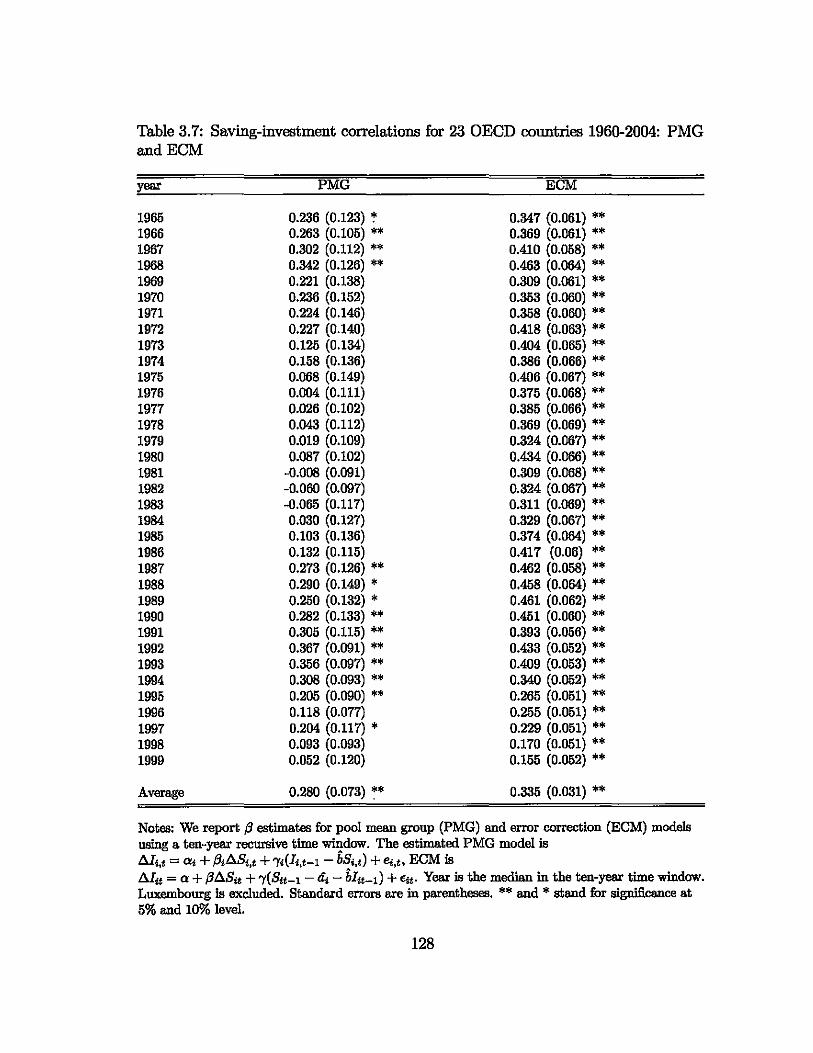
Table 3.7: Saving-investment correlations for 23 OEeD countries 1960-2004: PMG andECM
year PMG ECM
1965 0.236 (0.123) ~ 0.347 (0.061) ** 1966 0.263 (0.105) ** 0.369 (0.061) ** 1967 0.302 (0.112) ** 0.410 (0.058) ** 1968 0.342 (0.126) ** 0.463 (0.064) ** 1969 0.221 (0.138) 0.309 (0.061) ** 1970 0.236 (0.152) 0.353 (0.060) ** 1971 0.224 (0.146) 0.358 (0.060) ** 1972 0.227 (0.140) 0.418 (0.063) ** 1973 0.125 (0.134) 0.404 (0.065) ** 1974 0.158 (0.136) 0.386 (0.066) ** 1975 0.068 (0.149) 0.406 (0.067) ** 1976 0.004 (0.111) 0.375 (0.068) ** 1977 0.026 (0.102) 0.385 (0.066) ** 1978 0.043 (0.112) 0.369 (0.069) ** 1979 0.019 (0.109) 0.324 (0.067) ** 1980 0.OS7 (0.102) 0.434 (0.066) ** 1981 -O.OOS (0.091) 0.309 (0.068) ** 1982 -0.060 (0.097) 0.324 (0.067) ** 1983 -0.065 (0.117) 0.311 (0.069) ** 1984 0.030 (0.127) 0.329 (0.067) ** 1985 0.103 (0.136) 0.374 (0.064) ** 1986 0.132 (0.115) 0.417 (0.06) ** 1987 0.273 (0.126) ** 0.462 (0.058) ** 1988 0.290 (0.149) * 0.458 (0.064) ** 1989 0.250 (0.132) * 0.461 (0.062) ** 1990 0.282 (0.133) ** 0.451 (0.060) ** 1991 0.305 (0.115) ** 0.393 (0.056) ** 1992 0.367 (0.091) ** 0.433 (0.052) ** 1993 0.356 (0.097) ** 0.409 (0.053) ** 1994 0.308 (0.093) ** 0.340 (0.052) ** 1995 0.205 (0.090) *- 0.265 (0.051) ** 1996 0.118 (0.077) 0.255 (0.051) -* 1997 0.204 (0.117) - 0.229 (0.051) ** 1998 0.093 (0.093) 0.170 (0.051) ** 1999 0.052 (0.120) 0.155 (0.052) -*
Average 0.280 (0.073) ** 0.335 (0.031) **
Notes: We report p estimates for pool mean group (PMG) and error correction (ECM) models using a ten-year recursive time window. The estimated PMG model is AI;,t = a; + P.A8t,t + ')',(I"t-l - b8;,t) + e;,,, ECM is AI" = Q + PA8tt + ,),(8"-1 - If; - bItt-I) + <it. Year is the median in the ten-year time window. Luxembourg is excluded. Standard errors are in parentheses. ** and * stand for significance at 5% and 10% level.
128

coefficient between estimates using BN and PMG (ECM) is 0.53 (0.60), which is
higher than that using HP and PMG (0.44) or ECM (0.37). High correlation pro
vides additional support that difference models may render comparable estimation
results.
There are at least two potential explanations of the decreasing saving-investment
correlation before early 1980s. First, the breakdown of the Bretton Woods system
in early 70s pushed many industrial countries to remove capital control constraints,
which leads to a large capital mobility in OECD countries. And second, the oil
price shocks in 1973 and 1979 may have contributed to a drop in saving-investment
correlation. Jansen and Schulze (1996) explain why negative saving-investment cor
relation is likely to be found during the 1973 oil shock for the case of Norway. Their
main argument is that investment will increase when there is an oil price jump to in
crease future production and to exploit the profitability. But consumption also goes
up in anticipation of increasing revenues from this new source of income. Therefore
saving will temporarily drop down.
3.5 Conclusion
The purpose of this paper is to re-examine the FH puzzle by providing an alternative
measure of long-run and short-run correlations. We decompose saving and invest
ment into their permanent and transitory components, and run panel regressions
separately on two sets of components. By doing so, we are able to re-investigate the
outlier problem of Luxembourg and found that it is the long-run correlation, not the
short-run correlation, that led to remarkable under-estimation of saving-investment
129

c 0
I 0
Figure 3.4: Comparing short-run correlations from different models
1
0.8 (-./\
\ 0.6 \
\,
0.4 " ..
0.2 \/
o --PMG
-0.2 - - -ECM J .-'-'-'BN -HP
-0.4 '-==:::::C:~----'-__ .L...-_--,-_---,-__ -,---_--1 1965 1970 1975 1980 1985 1990 1995 2000
Year
Notes: PMG is pooled mean group estimator, which is a group-a.verage of short-run correlation estimates from regression M;" = ct; + "1(1.,'-1 - /,S;,,) + f3,ASi ,t + "',t where the long-run correlation /, is estimated from a POLS i!l the format of Ii" = a + bS"t + 'U;,t. ECM uses a pooled regression as in equation (3.2). BN (HP) correlation is defined as regression coefficient on transitory saving decomposed ueing BN (HP) method. Luxembourg is not included in the panel regression.
130
'.

correlation when BE and FE models are used. Monte Carlo simulation shows that
MG should probably be considered the best static panel estimator when multiple
factors, such as non-stationary, non-cointegrated variables, heterogeneity, and small
sample, need to be taken into account.
The short-run correlations estimated using traditional ECM and more recent
PMG model are generally found smaller than long-run correlations, but still signif
icantly different from zero. With our decomposition framework, we provide further
empirical evidence that the saving-investment correlation does have a smaller size
in the short-run than in the long-run. In addition, depending on the decomposition
method and the estimation model, the short-run correlation estimated under our
decomposition framework can be insignificantly different from zero. Comparative
studies show that BN decomposition method provides a more accurate description
of the dynamics of short-run correlation relative to traditional measures, than does
the HP filter. So the insignificant short-run correlation, estimated using BN de
composition and MG model, provides some tentative evidence that capital is very
mobile for DECD countries 1960-2004, if we believe that capital mobility is better
reflected in the short-run correlation.
As we said earlier in section 3.4.3, the main purpose of this paper is to exam
ine the magnitude of long-run and short-run correlation in a new decomposition
framework. However it would be interesting to further explore the question by
asking what explains long-run and short-run correlations. The marginal correla
tion between these two correlations apparently implies different mechanism working
beneath them. We will leave this interesting topic to future research project.
131

Appendix C.l Blancard and Quah (BQ) decom
position model
We show in this appendix that permanent and transitory components from BQ
decomposition model follow a similar path. Suppose that a bi-variate structural
VAR (SVAR) model in the format of
where Zt = [Xt Yt]', et = [€f ef]" and €f, ef are permanent and transitory shocks.
This SV AR model can be re-arranged and defined as a structural moving average
model (SMA)
where Do = A-l, and Dj = (A-l B)i A-l, Vj ;:: 1. The permanent component of Z,
Z[, is defined as that comes from permanent shock, therefore
Similarly transitory components of Z can be expressed as
132

w .... M~ [: : 1 w,=....ny_thattho_and_oompo-
nents of variable Z follow a very siinilar dynamic path, both having A -1 B as AR(1)
coefficient.
133

Bibliography
Abbott, Andrew J. and Glauco De Vita, "Another Piece in the Feldstein
Horioka Puzzle," Scottish Journo1 of Political Economy, 2003, 50 (1), 6989.
Als, G., "The Nightmare of Economic Accounts in a Small Country with A Large
International Banking Sector," Review of Income and Weo1th, 1988, 34, 101-
110.
Backus, David K., Patrick J. Kehoe, and Finn E. Kydland, "International
Real Business Cycle," Journal of Politico1 Economy, 1992, 100 (4), 745--774.
Baxter, Marianne and Mario Crucini, "Explaining Saving-Investment Corre
lations," American Economic Review, 1993, 83, 416-436.
Bayoumi, Tamim, "Saving-Investment Correlations: Immobile Capital, Govern
ment Policy, or Endogenous Behavior," IMF Staff Papers, 1990, 37,360-387.
Beauchemin, Kenneth and Betty Daniel, "Precautionary Saving, the Current
Account, and the International Distribution of Wealth," 2000. SUNY Working
paper.
Bebczuk, Ricardo and Klaus Schmidt-Hebbel, "Revisiting the Feldstein
Horioka Puzzle: An Institutional Sector View," 2006. MPRA Paper No. 1802.
134

Bergin, Pan! R. and Steven M. Sheifrin, "Interest Rates, Exchange Rates and
Present Value Models of the Current Account," The Economic Journal, April
2000, 110 (463), 535-558.
Blanchard, Olivier and Francesco Giavazzi, "Current Account Deficits in the
Euro Area: The End of the Feldstein-Horioka Puzzle?," Brvok:ings Papers on
Economic Activity, 2002, 2, 147-209.
Boileau, Martin, "'Irade in Capital Goods and Investment-Specific Technical
Change," 1999. Discussion Papers in Economics Woking Paper No.99-02, Cen
ter for Economic Analysis, Department of Economics, University of Colorado
at Boulder.
Bouakez, Hafedh and Takashi Kano, "Terms of Trade and Current Account
Fluctuations: The Harberger-Laursen-Metzler Effect Revisited," 2005. Work
ing paper.
Buiter, Willem H., "Time Preference and International Lending and Borrowing
in an Overlapping-Generations Model," Journal of Political Economy, 1981, 8
(4), 769-797.
Bussiere, Matthieu, Marcel Fratzscher, and Gernot J. Muller, "Productiv
ity Shocks, Budget Deficits and the Current Account," Augnst 2005. European
Central Bank Working Paper No.509.
Campbell, John and Robert Shiller, "Cointegration and Tests of Present Value
Models," Journal of Political Economy, 1987, 95 (5), 1062-1088.
Campbell, John Y. and N. Gregory Mankiw, "Permanent Income, Current
Income, and Consumption," 1989. NBER Working Paper No. 2436.
135

Caporale, Guglielmo Maria, Ekaterini Panopoulou, and Nikitas Pittis,
"The Feldstein-Horioka Puzzle Revisited: A Monte Carlo Study," Journal of
international Money and Finance, 2005, 24 (7), 1143--1149.
Cashin, Paul and C. John McDermott, "Terms of Trade Shocks and the Cur
rent Account: Evidence from Five Industrial Countries," Open Economies Re
view, 2002, 13,219235.
Cheung, Yin-Wong and Menzie D. Chinn, "Futher Investigation of the Uncer
tain Unit Root in GNP," Journal of Business and Economic Statistics, 1997,
15,68-73.
Choi, Horag, Nelson C. Mark, and Donggyu Sul, "The U.S. Current Account
and the Real Exchange Rate under Endogenous Subjective Discounting," Oc
tober 2005. Working Paper.
Christopoulos, Dimitris K. and Miguel Leon-Ledesma, "Current Account
Sustainability in the US: What Do We Really Know About It?," October 2004.
http://www.kent.ac. uk/ economics/papers/papers-pdf/2004/0412. pdf.
Clarida, Richard H., Manuela Goretti, and Mark P. Taylor, "Are There
Thresholds of Current Account Adjustment in the G7?," 2005. Working paper.
Clark, Peter K., ''The Cyclical Component of U. S. Economic Activity," Quarterly
Journal of Economics, 1987, J02 (4),797-814.
Coakley, Jerry, Ana-Maria Fuertes, and Fabio Spagnolo, "Is the Fe1stein
Horioka Puzzle History?," Manchester Schoo~ 2004, 72 (5), 569590.
136

_ , _ , and Ron Smith, "Small sample properties of panel time-series esti
mators with I(1) errors," 2001. Birkbeck College Discussion Paper No. 3/2001.
Cochrane, John H., "How Big Is the Random Walk in GNP?," Journal of Political
Economy, 1988, 96 (5), 893-920.
Coiteux, Martin and Simon Olivier, "The saving retention coefficient in the
long run and in the short run: evidence from panel data," Journal of Inte:ma
tional Money and Finance, 2000, 19 (4),535548.
Elliot, G., T. Rothenberg, and J. H. Stock, "Efficient Tests for an Autore
gressive Unit Root," Econometrica, 1996, 64,813-836.
Engle, Charles and John Rogers, "The U.S. Current Account Deficit and the
Expected Share of World Output," January 2006. NBER Working Paper
No.1l921.
Fattouh, Bassam, "Capital Mobility and Sustainability: Evidence from U.S. Cur
rent Account Data," Empirical Economics, 2005, 30, 245-253.
Feldstein, Martin, "Domestic Saving and International Capital Movements in the
Long Run and the Short Run," European Economic Rview, 1983, 21, 129--151.
_ and Charles Horioka, "Domestic Saving and International Capital Flows,"
Economic Journal, 1980, 90, 314-329.
Frankel, Jeffrey A., "Measuring International Capital Mobility: A Review,"
American Economic Review, 1992, 82 (2), 197-202.
137

Ghosh, Atish R., "International Capital Mobility Amongst the Major Industri
alised Countries: 'Tho Little or Too Much?," The Economic Journal, 1995, 105
(428), 107-128.
_ and Jonathan D. Ostry, "Macroeconomic uncertainty, precautionary sav
ing, and the current account," Journal of Monetary Economics, September
1997, 40 (1), 121-139.
Gil-Alana, L.A., ''Testing the Power of a Generalization of the KPSS-Tests against
Fractionally Integrated Hypotheses," Computational Economics, 2003, 22 (1),
23-38.
Glick, Reuven and Kenneth Rogoff, "Global versus Country-Specific Produc
tivity Shocks and the Current Account," Journal of Monetary Economics, 1995,
35, 159-192.
Gruber, Joseph W., "A present value test of habits and the current account,"
Journal of Monetary Economics, 2004, 51, 14951507.
Gruen, David W. R. and Jenny Wilkinson, "Australia's Real Exchange Rate
- Is it Explained by the Terms of Trade or by Real Interest Differentials?,"
Economic Record, 1994, 10 (2D9), 204-219.
Harberger, Arnold C., "Currency Depreciation, Income and the Balance of
Trade," Journal of Political Economy, 1950, 58,47-60.
Harvey, Andrew C., "Trends and Cycles in Macroeconomic Time Series," Journal
of Business & Economic Statistics, 1985, 3 (3), 216-227.
138

Herwartz, Helmut and Fang Xu, "Panel Data Model Comparison for Empirical
Saving-Investment Relations," 6 2006. Working paper.
Ho, Tsung-Wu, ''The Feldstein-Horiokapuzzle revisited," JOURNAL OF INTER
NATIONAL MONEY AND J:i'INANCE, 2002, 21 (4), 555564.
_ and Ru-Lin Chiu, "Country Size and Investment-Saving Correlation:A Panel
Threshold Error Correction Model," Eastern Economic Journal, 2001, 27 (4),
481-490.
Hobijn, Bart, Philip Hans Franses, and Marius Ooms, "Generalizations of
the KPSS-test for Stationarity," 1998. DiscllBSion Paper 9802, Econometric
Institute, ErllBIIlus University Rotterdam.
Huang, Chao-His and Kenneth S. Lin, "Deficits, Government Expenditures
and Tax Smoothing in the United States: 1929-1988," Journal of Monetary
Economics, 1993, 31, 317-339.
Hussein, Khaled A., "International Capital Mobility in OECD Countries: The
FeldsteinHorioka Puzzle Revisited," Economics Lette:rs, 1998, 59, 237242.
Iscan, Talan B., "Present Value Tests of the Current Account with Durables
Consumption," June 1999. Dalhousie University Working paper.
_ , "The Terms of Trade, Productivity Growth and the Current Account," Jour
nal of Monetary Economics, 2000, 45, 587-611.
Jansen, W. Jos, "Estimating Saving-Investment Correlations: Evidence for OECD
Countries Based on An Error Correction Model," Journal of International
Money and Finance, 1996, 15 (5), 749--781.
139

_, "Can the Intertemporal Budget Constraint Explain the Feldstein-Horioka
Puzzle?," Economics Letters, 1997, 56 (1), 77--83.
_, ''Interpreting Saving-Investment Correlations," Open Economies Review,
1998, 9, 205--217.
_ , "International capital mobility: evidence from panel data," Journal of Inter
national Money and Finance, 2000, 19 (1), 507511.
Jansen, W Jos and Gunther G. Schulze, "Theory-Based Measurement of the
Saving-Investment Correlation with An Application to Norway," Economic In
quiry, 1996, 34 (1), 116--131.
Johansen, Soren, Likelihood-Based Inference in Cointegrated Vector Autoregres
sive Models, Oxford University Press, New York, 1995.
Kana, Takashi, "Habit Formation, the World Real Interest Rate, and the Present
Value Model of the Current Account," 2003. mimeo.
Kent, Christopher, "The Response of the Current Account to Terms of Thade
Shocks: A Panel-Data Study," 1997. Research Discussion Paper 9705, Ec0-
nomic Research Department, Reserve Bank of Anstralia.
Kim, Sunghyun Henry, "The Saving-Investment Correlation Puzzle is Still a
Puzzle," Journal of International Money and Finance, 2001, 27 (7), 1017-1034.
Krol, Robert, "International capital mobility: evidence from panel data," Journal
of International Money and Finance, 1996, 15 (3), 467-474.
Kwiatkowski, D., P. Phillips, P. Schmidt, and Y. Shin, ''Testing the Null Hy
pothesis of Stationarity Againffi; the Alternative of a Unit Root: How Sure Are
140

We that Economic Times Series Have a Unit Root?," Journal of Econometrics,
1992, 54, 159--178.
Laursen, Svend and Lloyd A. Metzler, "Flexible Exchange Rates and the
Theory of Employment," The Review of Economics and Statistics, 1950, 32
(4),281-299.
Mamingi, NIandu, "Saving-Investment Correlations and Capital Mobility: The
Experience of DeveIoping Countries," Journal of Policy Modeling, 1997, 19 (6),
605-626.
Marquez, Jaime, "Productivity, Investment, and Current Accounts: Reassess
ing the Evidence," November 2002. International Finance Discussion Papers
Number 742.
Matsubayashi, Yoichi, "Are US Current Account Deficits Unsustainable? 'Thsting
for the Private and Government Intertemporal Budget Constraints," Japan and
the World Economy, April 2005, 17 (2), 223--237.
Matsuyama, Kiminori, "Terms-of-Trade, Factor Intensities and the Current Ac
count in a Life..Cycle Model," Review of Economic Studies, 1988, 55,247-262.
Mendoza, Enrique G., ''The Tepns of Trade, the Real Exchange Rate, and Ec0-
nomic Fluctuations," International Economic Review, 1995, 36 (1), 101-137.
Mercereau, Benoit and Jacques Miniane, "Challenging the Empirical Evidence
from Present Value Models of the Current Account," June 2004. IMF Working
Paper WP /04/106.
141

Moosa, Imad A., "A Note on Capital Mobility," Southern Economic Journo1,
1996, 63 (1), 248-254.
Morley, James C., Charles R. Nelson, and Eric Zivot, "Why Are the
Beveridge-Nelson and Unobserved-Components Decompositions of GDP So
Different?," The Review of Economics and Statistics, 2003, 85 (2),235-243.
Murray, Christian J. and Shushanik Papanyan, "The Relative Importance
of Permanent and Transitory Components in Macroeconomic Time Series,"
November 2004. Working paper.
Nason, James M. and John H. Rogers, "Investment and the Current Account
in the Short Run and Long Run," Journo1 of Money, Credit, and Banking,
2002, 34 (4), 967-986.
_ and _ , ''The Present-Value Model of the Current Account Has Been Re
jected: Round Up the Usual Suspects," February 2003. International Finance
Discussion Papers Number 760.
Obstfeld, Maurice, "Aggregate Spending and the Terms of Trade: Is There a
Laursen-Metzler Effect?," Quarterly Journal of Economics, 1982, 97, 251-270.
_, "Capital Mobility in the World Economy: Theory and Measurement,"
Carnegie-Rochester Conference Series on Public Policy, 1986, 31, 1-24.
_ and Kenneth Rogoff, The Handbook of Internationo1 Economics, Vol. 3,
Elsevier,
_ and __ , "Perspectives on DECD Economic Integration: Implications for
US Current Account Adjustment," September 2000. Working Paper.
142

_ and _, "The Six Puzzles in International Macroeconomics: Is There a
Common Cause?," 2000. NBER Working Paper No. 7777.
Otto, Glenn, "Testing A Present-Value Model of the Current Account: Evidence
from US and Canadian Time Series," Journal of International Money and Fi
nance, 1992, 11, 414--430.
_, "Terms of Trade Shocks and the Balance of Trade: There is a Harberger
Laursen-Metzler Effect," Journal of International Money and Finance, 2003,
22, 155-184.
Pelgrin, Florian and Sebastian Schich, "National SavingInvestment Dynamics
and International Capital Mobility," 2004. Bank of Canada Working Paper
2004-14.
Pesaran, M. Hashem and Ron P. Smith, "Estimating Long-run Relationships
from Dynamic Heterogeneous Panels," Journal of Econometrics, 1995, 68, 79-
113.
Philips, Peter C. B. and Hyurigsik R. Moon, "Linear Regression Limite The
ory for Nonstationary Panel Data," Econometrica, 1999, 67 (5), 1057-1111.
Sachs, Jeffrey, "The Current Account and Macroeconomic Adjustment in the
19708," Brookings Papers on Economic Activity, 1981, 12,201-268.
Sarno, Lucio and Mark P. Taylor, "Savings-investment correlations: Transitory
versus permanent," Manchester School, 1998, 66, 17-38.
143

Schmidt, Caroline, "Saving-Investment Correlations in Response to Mone
tary Policy Shocks: New Insights into the Feldstein-Horioka Puzzle?," Open
Economies Review, 2007, 18 (3), 347-367.
Sen, Partha and Stephen J. Turnovsky, "Deterioration of the Terms of Trade
and Capital Accumulation: A Re-Examination of the Laursen-Metzler Effect,"
Journal of International Economics, 1989, 26, 227-250.
Serven, Luis, "Terms-of-Trade Shocks and Optimal Investment: Another Look
at the Laursen-Metzler Effect," Journal of International Money and Finance,
1999, 18 (3), 337-365.
Sheffrin, Steven M. and Wing Thye Woo, "Present Value Tests of An Intertem
poral Model of the Current Account," Journal of International Economics,
1990, 29, 237-253.
Shibata, Akjbjsa and Mototsugu Shintani, "Capical Mobility in the World
Economy: An Alternative Test," Journal of International Money and Finance,
1998, 17, 741-756.
Stockman, Alan C. and Linda L. Tesar, ''Tastes and Technology in a Two
Country Model of the Business Cycle: Explaining International Comovements,"
American Economic Review, 1995, 85, 168-185.
Sundaresan, Suresh M., "Intertemporally Dependent Preferences and the Volatil
ity of Consumption and Wealth," Review of Financial Studies, 1989, 2 (1),
73-89.
144

Svensson, Lars E. O. and Assaf Razin, "The Terms of Trade and the Current
Account: The Harberger-Laursen-Metzler Effect," Journal of Political Econ
omy, 1983, 91, 97-125.
Taylor, Alan M., "International Capital Mobility in History: The Saving
Investment Relationship," 1997. NBER Working Paper No.5743.
Wen, Yi, "By Force of Demand: Explaining International Comovements," Journal
of Economic Dynamics and Control, 2007, 91, 1-23.
145