Universita degli Studi di Roma ‘Tor Vergata’Dottorato di ricerca in Matematica (XV ciclo)

PhD Thesis

Diffusive behaviorand asymptotic self similarity

for fluid models

Author: Marco Di Francesco

Advisor: Pierangelo Marcati

June 2004

Abstract

The present PhD thesis deals with diffusive relaxation limits and long timeasymptotics for several partial differential equations or systems of equationsof hyperbolic or parabolic type. Most of the models considered arise fromcompressible gas dynamics; some of them take into account of heat radiationphenomena, some others involve the presence of porous media. We make useof classical techniques, such as Friedrichs symmetrization for quasi linear hy-perbolic systems and energy estimates, as well as of more recently developedtools, such as the entropy dissipation method and the optimal transportationapproach.

i

Acknowledgments

This PhD thesis owes a lot to many people. I mention above all Piero Marcatiand Corrado Lattanzio, who both have helped me with stimulating discus-sions and useful comments and ideas to improve my work. Then, I wouldlike to thank Bruno Rubino and Donatella Donatelli for frequent and usefuldiscussions with them.

I had the honor and the pleasure to be introduced in the study of thetopics in chapters 5 and 7 by Peter A. Markowich, Giuseppe Toscani andJose A. Carrillo.

I am grateful to Piero Marcati for having introduced me in the study ofapplied mathematics.

ii

Contents

1 Introduction 11.1 General outline . . . . . . . . . . . . . . . . . . . . . . . . . . 11.2 Relaxation limits for hyperbolic models. . . . . . . . . . . . . 21.3 The Euler equations for compressible gas dynamics . . . . . . 51.4 Diffusive relaxation model for a system of viscoelasticity . . . 81.5 The Hamer model for radiating gases . . . . . . . . . . . . . . 101.6 Nonlinear diffusion phenomena. The porous medium equation. 141.7 The entropy dissipation method . . . . . . . . . . . . . . . . . 161.8 The viscous Burgers’ equation . . . . . . . . . . . . . . . . . . 191.9 The Wasserstein distance . . . . . . . . . . . . . . . . . . . . . 20

I Relaxation limits 22

2 The compressible Euler equations with damping 232.1 Statement of the problem and results . . . . . . . . . . . . . . 232.2 The Proof of the main Theorem . . . . . . . . . . . . . . . . . 27

3 A one dimensional model for viscoelasticity 393.1 Global existence and singular convergence of H1 solutions . . . 393.2 Rate of convergence in L2 norm . . . . . . . . . . . . . . . . . 443.3 Travelling waves . . . . . . . . . . . . . . . . . . . . . . . . . . 47

4 The Hamer model for radiating gases 534.1 Global existence of solutions . . . . . . . . . . . . . . . . . . . 53

4.1.1 Well–posedness via nonlinear semigroups . . . . . . . . 624.1.2 Extension to L∞ . . . . . . . . . . . . . . . . . . . . . 67

4.2 Relaxation Limits . . . . . . . . . . . . . . . . . . . . . . . . . 684.2.1 Hyperbolic-hyperbolic relaxation limit . . . . . . . . . 684.2.2 Hyperbolic-parabolic relaxation limit . . . . . . . . . . 74

iii

II Long time asymptotics 80

5 Nonlinear diffusion equations 815.1 Preliminaries . . . . . . . . . . . . . . . . . . . . . . . . . . . 815.2 The relative entropy method . . . . . . . . . . . . . . . . . . . 84

5.2.1 Statement of the problem and result . . . . . . . . . . 845.2.2 Proof of Theorem 5.2.3 . . . . . . . . . . . . . . . . . . 88

5.3 Evolution of the 1-d Wasserstein distances . . . . . . . . . . . 905.3.1 Preliminaries and results . . . . . . . . . . . . . . . . . 905.3.2 Proof of Theorem 5.3.1 . . . . . . . . . . . . . . . . . . 94

6 A small perturbation result for nonlinear diffusion far fromvacuum 986.1 Statement of the problem and result . . . . . . . . . . . . . . 986.2 The Proof of the Theorem 6.1.1 . . . . . . . . . . . . . . . . . 100

7 The viscous Burgers Equation 1037.1 The Hopf–Cole Transformation . . . . . . . . . . . . . . . . . 103

7.1.1 The classical setting . . . . . . . . . . . . . . . . . . . 1037.1.2 Intermediate asymptotics and zero–viscosity

regime . . . . . . . . . . . . . . . . . . . . . . . . . . . 1057.1.3 The time–dependent scaling . . . . . . . . . . . . . . . 107

7.2 Trend to equilibrium in relative entropy . . . . . . . . . . . . . 1097.3 Evolution of the Wasserstein metric . . . . . . . . . . . . . . . 119

8 A stability result for radiating gases 1248.1 Statement of the problem and result . . . . . . . . . . . . . . 1248.2 Proof of the main theorem . . . . . . . . . . . . . . . . . . . . 128

A Uniqueness and regularity of Hs solutions for a hyperbolic–parabolic system 132

B Local existence for the vanishing viscosity approximation ofthe Hamer model for radiating gases 137

References 141

iv

Chapter 1

Introduction

1.1 General outline

The present PhD thesis is concerned with the asymptotic analysis of hyper-bolic and parabolic partial differential equations and systems of equations,mainly models in continuum mechanics and physics such as compressiblegas–dynamics, flow through porous media, motion of radiating gases, vis-coelastic materials, general nonlinear diffusion phenomena. The present the-sis is devoted to investigate qualitative properties of the solutions of initialvalue problems for the previously mentioned models, in one or several spacedimension. More precisely, we focus our attention mainly on two kinds ofproblems:

(i) The former regards the analysis of the limiting behavior of solutionswith respect to some singular parameter appearing in the model. Thisparameter may arise either from relaxation phenomena or as a result ofan internal rescaling. In both the cases, our strategy is to determine anequilibrium or limit problem, then to justify rigorously the convergenceprocess.

(ii) The latter concerns with the analysis of the long time behavior of thesolutions and the appearance of intermediate asymptotic states enjoy-ing a self–similar structure. In most of the models studied, we will bealso interested in determining the optimal rate of convergence in someLp or Sobolev spaces.

The link between (i) and (ii) can be intuitively understood by meansof the following example, representing a simplified model for radiation gas

1

dynamics (we will analyze this model in Chapters 4 and 8)ut + uux = −qx−qxx + q = −ux.

(1.1)

In this case (as in many more cases throughout our work), the rescalingprocess we perform in order to detect the an asymptotic approximation is ofthe form

uε(x, t) =1

εu

(x

ε,t

ε2

), qε(x, t) =

1

ε2u

(x

ε,t

ε2

). (1.2)

Here the formal limit is represented by the viscous Burgers’ equation forthe variable u (we skip the details, see Chapter 4). Hence, since the scalingfactor for the time variable t grows faster than the scaling factor for thespace variable x as ε approaches zero, one can pose the problem of detecting adiffusive limiting behavior also in a framework of pure long time asymptotics.

This introductive chapter is organized as follows. In the section 1.2 weexplain some basic ideas of relaxation limits for hyperbolic problems, by fo-cusing in particular on the diffusive relaxation limits. In the section 1.3 weshall discuss one of the most classical models which motivates the study ofdiffusive relaxation hyperbolic systems, namely the Euler equations of com-pressible fluids thorugh of porous media. In the section 1.4 we introduce arelaxation model for viscoelasticity, and in the section 1.5 we shall give abrief introduction to the mathematical theory for the models in radiationgas dynamics. The section 1.6 is devoted to the porous medium equation,while the section 1.7 will provide an outline of the entropy methods recentlyused to analyze the long time asymptotics for nonlinear diffusion equations.The section 1.8 contains an introduction to another simplified model forcompressible gas dynamics, i.e. the viscous Burgers’ equation. Finally, thesection 1.9 is devoted to another tool used recently in the study nonlineardiffusion, i.e. the Wasserstein distance. In our introduction, the most im-portant results contained in the present thesis will be presented and framedinto their natural context. We remark that the references reported here areobtained as the result of a selection done in relation with the topics and withthe results contained in this thesis. Hence, the literature presented later willbe not complete and will not appropriately describe the general subject.

1.2 Relaxation limits for hyperbolic models.

Relaxation phenomena arise typically in cases of perturbations of an equi-librium state for a given physical model. The simplest cases is the following

2

linear hyperbolic systemut + vx = 0

vt + λux = 1ε(αu− v) ,

where the equilibrium is represented by the equation

ut + αux = 0

and by the relationαu− v = 0.

In this simple case a straightforward computation shows that the convergencetowards equilibrium occurs if and only if λ2 ≥ α2 (this is known as the sub-characteristic condition). The typical general form for a hyperbolic systemswith relaxation in the framework of smooth solutions is the following,

∂tU +d∑j=1

Aj(U)∂xjU =

1

εQ(U) (1.1)

where the unknown U is a function of x ∈ Rd and t ≥ 0 with values in an opensubset A of Rk, Aj and Q are smooth functions of U . The quasi linear systemabove is usually supposed to be symmetrizable hyperbolic in the sense ofFriedrichs (see [Fri54, Maj84]), i.e. there exists a symmetric positive definitematrix valued function A0(U) that symmetrizes simultaneously Aj(U) for allj = 1, . . . , d (see [Fri54, Lax57, Kat75, Maj84]).

The source term 1εQ(U) is often referred to as the relaxation term. This

term is supposed to be endowed with two operators. The first one, whichwe denote by P , is called the projection on the momenta. In a simplifiedsituation, P can be assumed to be a constant linear operator from Rk to Rn

with n < k, such that PQ(U) = 0 for all U ∈ A. This structural assumptionexpress the fact that n equations in system (1.1) can be rewritten in thehomogeneous form

∂tPU +d∑j=1

PAj(U)∂xjU = 0.

The second operator is a map M defined on an open set of Rn with valuesin Rk (often called the Maxwellian operator) such that QM(u) = 0 andPM(u) = u. Under certain hypothesis (see [Nat99] for further details), onemay expect that the unknown U converges in some sense, as ε → 0, to the

3

equilibrium M(u) where the vector valued function u satisfies the reducedsystem

∂tu+d∑j=1

PAj(M(u))∂xjM(u) = 0.

A quite general theory for these kinds of systems has been recently developedby W.A. Yong (see [Yon99]). There exist then a large variety of interestingphysical examples where relaxation schemes can be applied, such as singu-lar perturbations of the wave equation, traffic flow models, and the kineticBroadwell model. For a detailed explanations of these models we refer tothe survey paper by Natalini [Nat99], where also a huge list of referencescan be found, together with detailed proofs of more recent and advancedresults on these topics. One of the main scopes of relaxation schemes is toconstruct admissible weak solutions to the reduced hyperbolic equations orsystems. A typical case is the relaxation towards a scalar conservation laws(see [Nat99, Daf00] and the references therein). In this sense, this approachis quite similar to the kinetic formulation of a conservation law (see [Daf00]).For the basic theory of linear relaxation schemes we refer to the pioneeringbook by Whitham [Whi74]. The corner stone for the nonlinear theory is thefundamental paper by Tai Ping Liu [Liu87] (see also [CLL94]).

In the recent years, hyperbolic systems relaxing towards diffusive modelshave been the subject of a wide investigation. A very simple (linear) examplein this sense is provided by the dissipative wave equation

utt −∆u+1

εut = 0.

By rescaling a solution to that equation as follows

u(x, t) =1

εv

(x,t

ε

),

it can be proven that v converges (e.g. in Hs) to the solutions of the linearheat equation vt = ∆v. We explain hereafter the basic ideas of diffusiverelaxation processes, without taking care of all the structural assumptionsand the technical details, for which we refer to the paper by Marcati andRubino [MR00]. Let us consider a quasi linear hyperbolic system in vectorform

Ut + F (U, V )x = 0

Vt +G(U, V )x = H(U, V )

We then perform the parabolic scaling

U ε(x, t) = U

(x√ε,t

ε

)V ε(x, t) =

1√εV

(x√ε,t

ε

)(1.2)

4

for any ε > 0. Then, by substituting the new variables into the originalsystem and by taking the formal limit as ε → 0 (under more structuralassumptions), see [MR00]), one recovers the reduced system

Ut + (FV (U, 0)V )x = 0

G(U, 0)x = HV (U, 0)V

Under the extra assumption detHV (U, 0) 6= 0, one can rewrite the abovereduced system as

Ut +(FV (U, 0) (HV (U, 0))−1G(U, 0)x

)x

= 0,

which is a parabolic system in the sense of Petrowski (see the book of Kreissand Lorentz [KL89]).

The parabolic scaling we use here is the classical transformation one needsto apply to a nonhomogeneous hyperbolic system to detect its parabolic be-havior time–asymptotically. Among all, in this framework, we recall thepapers of Kurtz [Kur73] and McKean [McK75], where for the first time thisfeature for hyperbolic systems has been put into evidence. Afterwards, werecall the papers of Marcati with various collaborators (see [MR00, DM00]and the references therein), where the above scaling has been used for severalsystems and the convergence has been obtained for weak solutions with theaid of the compensated compactness. Moreover, we recall the paper of Lionsand Toscani [LT97], where the same parabolic behavior has been pointed outfor Boltzmann kinetic models with a finite number of velocities, proving inparticular the convergence towards the porous media equation. In [LN02],the authors proposed a BGK approximation for strongly parabolic systemsverifying certain conditions and they proved the convergence of weak solu-tions, again using compensated compactness. The study of Hs solutions,with a detailed analysis of the initial layer phenomenon, has been carriedout in [LY01], for hyperbolic relaxation systems with a strongly parabolicequilibrium system.

1.3 The Euler equations for compressible gas

dynamics

The inviscid flow of a compressible fluid is described by the Euler equationsρt + div(ρu) = 0

(ρu)t + div(ρu⊗ u+ pI) = 0ρ(e+ |u|2

2

)t+ div

ρu(e+ |u|2

2

)+ pu

= 0,

(1.1)

5

where the three equations express conservation of mass, momentum and en-ergy respectively. We refer to the book of Courant and Friedrichs [CF48] fora detailed derivation of several models in compressible gas–dynamics. Thestudy of system (1.1) is a classical topic. Such system enjoys a quasi–linearsymmetric hyperbolic structure, in such a way that the local–in–time ex-istence of Hs solutions is guaranteed by the existence of a Friedrichs typesymmetrizer (see Friedrichs [Fri54] and the book of Majda [Maj84]). Then,the formation of shock waves in finite time may occur. This phenomenon isbest understood in one space dimension, where the method of characteris-tics can be employed (see Courant–Friedrichs [CF48] and Whitham [Whi74]).The formation of singularities in several space variables has been the topic ofmore recent investigations, see [Sid85, Sid91, Sid97, MUK86, Ali93, Ali95].

In Chapter 2 we will concern with a class of smooth solutions to the oned-imensional isentropic compressible inviscid Euler equations through porousmedia. In this case, a dissipative nonhomogeneous term in the balance lawof the momentum appears, because of the friction due to the presence of aporous medium. The model then readsρτ + (ρu)x = 0

uτ + uux +p(ρ)xρ

= −uε.

(1.2)

As was first proven by Nishida (see [Nis68]), the presence of the damping term−uε

prevents the formation of singularities for small initial data belonging incertain Sobolev spaces (of course the smallness needed to preserve regularitydepends on the amplitude of the positive parameter ε). This result has beenonly recently extended to the three dimensional case in the paper [STW03].In both cases, to ensure global existence and smoothness of the solutions, anabstract continuation principle must be satisfied (see [Maj84] for its preciseformulation), which is basically a global (w.r.t. to time) energy estimatefor the space derivatives of the solutions up to a certain order. In Chapter2 we will show, in particular, that the global–in–time existence of smoothsolutions for system (1.2) can be extended to small perturbations of a specialclass of diffusion waves (see Remark 2.1.3).

After the scaling

ρε(x, t) = ρ(x, t/ε) uε(x, t) =1

εu(x, t/ε),

system (1.2) can be rewritten as followsρεt + (ρεuε)y = 0

uεt + uεuεy +p(ρε)yε2ρε

= −uε

ε2.

(1.3)

6

Hence, the density ρε formally converges as ε → 0 to a solution of the non-linear diffusion equation ρt = p(ρ)xx. This was first proven by Marcati andMilani in [MM90] in a framework of weak solutions, by means of techniquesbased upon compensated compactness tools. This paper provided a contri-bution in understanding the hyperbolic nature of porous media flows. Let usremark that the previous scaling, even though apparently different from theusual parabolic scaling (1.2), gives raise to the same reduced system even inthe general framework of diffusive relaxation limits (see the introduction to[MR00]).

The study developed in Chapter 2 goes in the same direction as [MM90],but in a context of smooth solutions, as already pointed out before. Inthe present case, we have to do with solutions far from vacuum, i.e. suchthat ρ ≥ ρ > 0. In particular, the initial data must satisfy certain limitingconditions at ±∞ in order to ensure absence of vacuum for large x. We willstudy the behavior of the solutions as the parameter ε goes to zero, and showthat, under some assumption on the initial data and on the limiting statesat infinity, the density in (1.3) converges in a suitable norm to a caloric selfsimilar solution to the generalized Porous Medium equation (see also Section1.6)

ρt = p(ρ)yy. (1.4)

Such solutions depend only on the similarity variable x/t1/2, and satisfy thesame limiting conditions as the density in (1.3). The existence of such caloricself–similar solutions has been the subject of many papers starting from theseventies, see [AP71, AP74, vDP77, vDP77]. We will show in Chapter 6 thatthese caloric profiles are asymptotically stable states for equation (1.4) if theinitial datum is a small perturbation of them.

We remark that our result holds in a well–prepared initial data regime,i.e. the initial data satisfy the equilibrium relation

p(ρ)x = −ρu,

which in this case is known as Darcy’s law. In this sense, we do not deal withthe so called initial layer problem, which is one of the main issues of someother papers in the literature (see Lattanzio and Yong [LY01] e.g.).

Besides what mentioned above for the compressible Euler system, a par-allel study of the asymptotic behavior for large times for the damped com-pressible Euler flow, both in Lagrangian and in Eulerian coordinates, hasbeen developed by Hsiao and Liu [HL92], [HL93] and by Nishihara [Nis96],where the above mentioned caloric self similar profiles were recovered to beasymptotically stable states under small perturbations for the damped oned-

7

imensional p–system ut − vx = 0

vt − p(u)x = −v(1.5)

Moreover, a result concerning the 2-D perturbation of this problem wasproved by Lattanzio and Marcati in [LM99]. Recently in [NWY00], Nishi-hara, Wang and Yang proved a sharper result on the Lp–convergence (2 ≤p ≤ ∞) by means of a Green function technique. We also mention [MP01],in which an analogous result is proven for a compressible adiabatic flow, and[MN03], where the authors recover sharp Lp–Lq estimates for the dampedwave equation and apply them to the asymptotic study of the damped p–system (1.5). The book by Hsiao [Hsi97] collects many results in these di-rections, most of them are based on energy estimate and Green functionstechniques and hold in a small perturbation setting. In Eulerian coordi-nates, the first convergence result to self similar solutions including vacuumhas been carried out in [HMP]. We remark that although in both the Eule-rian and the Lagrangian case the limiting profiles satisfy the Porous Mediaequation, the two cases cover different physical situations.

The results in Chapter 2 are contained in the author’s paper (joint withMarcati) [DFM02]. In particular, a convergence result in Sobolev norm hasbeen proven under the assumption of well prepared initial data. The tech-nique used is based on the standard symmetric hyperbolic systems frameworkdeveloped by Friedrichs, Lax, Majda and many more in [CF48, Lax57, KM81,KM82, Maj84].

1.4 Diffusive relaxation model for a system

of viscoelasticity

We analyze here the following semilinear hyperbolic system with relaxationterm

Us − Vy = 0

Vs − Zy = 0

Zs − µVy = −Z + ε2σ(U),

(1.1)

where U , V , Z ∈ R, y ∈ R, s > 0, µ is a strictly positive parameter and ε > 0denotes the relaxation time. Our goal is to detect the diffusive relaxationlimit for the system (1.1) as ε ↓ 0. To perform this task, we scale both thedependent and the independent variables with respect to the relaxation time

8

ε in the following way

u(x, t) = U

(x

ε,t

ε2

)v(x, t) =

1

εV

(x

ε,t

ε2

)z(x, t) =

1

ε2Z

(x

ε,t

ε2

).

With the above diffusive scaling, the system (1.1) becomesut − vx = 0

vt − zx = 0

ε2zt − µvx = −z + σ(u),

(1.2)

which, with ε = 0, formally reduces tout − vx = 0

vt − σ(u)x = µvxx.(1.3)

In Chapter 3 we will prove that solutions of (1.2) converge to solutions of(1.3), giving in this way a rigorous justification of the relaxation limit.

We shall assume the function σ in the relaxation term of (1.2) to beglobally Lipschitz, namely

supu∈R

|σ′(u)| < +∞. (1.4)

We recall that condition (1.4) represents the soft hardening condition forthe stress–strain function σ in system (1.3). Moreover, at this stage we donot need to require the positivity of σ′, namely we can approximate alsoincompletely parabolic systems where the corresponding inviscid first ordersystem is not necessarily hyperbolic. We emphasize this is the first rigorousproof of a relaxation limit from a hyperbolic toward an hyperbolic parabolicsystem.

This semilinear relaxation approximation has another physical interpre-tation in terms of mathematical models in the study of viscoelastic materials[RHN87]. Indeed, the system (1.2) can be rewritten as follows

ut − vx = 0

vt − zx = 0(z − µ

ε2u)t= − 1

ε2(z − σ(u)) ,

(1.5)

that is, a system of viscoelasticity with memory. In the system (1.5), thestress function z is given by the following relation

z =µ

ε2u−

∫ t

−∞

1

ε2e−

t−τ

ε2

( µε2u− σ(u)

)(τ)dτ,

9

while in the limit (1.3), the stress is given by the relation

z = σ(u) + µvx,

which is the case of viscoelasticity of the rate type. Therefore, our relaxationlimit can be viewed as the passage from the viscosity of the memory type tothe viscosity of the rate type in the study of viscoelastic materials. To detectthis phenomenon, in the definition of the stress z, we scale either the kernelof the memory, and the (linear) elastic response of the material at initialtime. Here we recall that the case of a fixed response of the material, whichcorresponds to a hyperbolic scaling of the relaxation approximation, has beenstudied in [Tza99], where the convergence toward the 2×2 hyperbolic systemof elasticity has been proved.

The results collected in Chapter 3 are the subject of the author’s paper(joint with Lattanzio) [DFL].

1.5 The Hamer model for radiating gases

A quite general model for compressible gas dynamics where heat radiativetransfer phenomena are taken into account is given by the hyperbolic ellipticcoupled model

ρt + div(ρu) = 0

(ρu)t + div(ρu⊗ u+ pI) = 0ρ(e+ |u|2

2

)t+ div

ρu(e+ |u|2

2

)+ pu+ q

= 0

−∇ div q + aq + b∇T 4 = 0.

(1.1)

As usual, in (1.1), ρ, u, p, e and T are respectively the mass density, velocity,pressure, internal energy and absolute temperature of the gas, while q isthe radiative heat flux and a and b are given positive constants dependingon the gas itself. We give here a sketch of the physical motivation of thefourth equation in (1.1) (see the books by Vincenti and Kruger [VK65] andby Zel’dovich and Raizer [ZR66] for a detailed explanation), the first threeequations being motivated as for the usual Euler system (see [CF48]).

We start from the physical observation that high temperature gases emitenergy in the form of electromagnetic radiation. This is due both to transi-tions from upper to lower energy levels of the atoms or molecules of the gasand from transitions that involve free electrons. We consider radiation fieldsas composed by photons, each one of them has energy and moves with lightspeed c. The spectral radiation intensity, then, can be expressed as

Iν(r,Ω, t)dνdΩ = hνcf(ν, r,Ω, t)dνdΩ,

10

where f(ν, r,Ω, t) is the number of photons in the frequency interval [ν, ν +dν], in the unit volume dr, within the solid angle dΩ, at time t, and h is thePlanck constant. The spectral energy flux reads

qν(r, t) =

∫IνΩdΩ.

Hence, by writing down the kinetic equation for Iν one recovers the followingradiative heat transfer equation

1

c

[∂Iν∂t

+ cΩ · ∇Iν]

= jν

(1 +

c2

2hν3Iν

)− kνIν , (1.2)

where the gradient is taken with respect to r and where the right hand sideis the difference between the emitted radiation and the absorbed radiation.Since the photons obey to Bose–Einstein statistics at the equilibrium, thestationary distributions in the equation (1.2) are represented by

I∗ν =2hν3

c2

(1

ehν/kT − 1

),

where k is the Boltzmann constant and T the temperature. Under the as-sumption of quasi equilibrium approximation, equation (1.2) reads

div (ΩIν) = αν [I∗ν − Iν ] ,

with α = ρkν(1− e−hν/kT

). After integration with respect to Ω ∈ S2 and

with respect to ν ∈ [0,+∞) we obtain

div q = −α(I − 4σT 2

),

where we have set

I =

∫ ∫Iν(Ω)dνdΩ, q =

∫ ∫ΩIν(Ω)dνdΩ,

for suitable constants α and σ. Under another extra assumption on themodel, namely the so called Milne–Eddington approximation∫ ∫

ΩiΩjIν(Ω)dνdΩ =1

3δij

∫ ∫IνdΩ

(see [VK65, ZR66]), we finally obtain

−∇ div q + 3α2q + 4σα∇T 4 = 0, (1.3)

11

which is exactly the fourth equation in the system (1.1).The model (1.1) has a simplified version, namely

ut + a · ∇u2 = − div q

−∇ div q + q = −∇u(1.4)

where u = u(x, t) ∈ R, q = q(x, t) ∈ R3 x ∈ R3, t ≥ 0 and a is a constant vec-tor. The simplified model (1.4) was first recovered by Hamer (see [Ham71]).The most convenient approach to such system is to solve the elliptic equa-tion satisfied by the term div q in terms of u and substitute it into the firstequation in order to get the scalar balance law

ut + a · ∇u2 = −u+K ∗ u, (1.5)

where the kernel K is given by the Bessel potential

K(x) =1

(4π)d/2

∫ +∞

0

e−s−|x|24s

sd/2ds

In one space dimension, equation (1.5) was first studied in [ST92], where theauthors referred to it as the Rosenau–Chapman–Enskog equation, and succes-sively in [LM03]. In particular, it has been proven that this equation inducesa contraction semigroup in Lp, p ∈ [1,∞] for all positive times, and it has acritical threshold (in terms of Sobolev norms) below which it preserves theregularity of the initial datum. This is essentially proven by taking advantageof the dissipative nature of the inhomogeneous term −u +K ∗ u. Concern-ing the general model (1.1) and its simplified version (1.4), the study of theexistence of smooth solutions, together with the existence and stability ofshock profiles in one space dimension has been perfomed by Kawashima andvarious collaborators in the general context of quasi linear hyperbolic ellipticcoupled systems (see [KN98, KN99a, KN99b, KNN99, KN02, KNN03]), andby Serre (see [Ser, Ser03]). In Chapter 4 we extend the global well–posednessof the model to the case of several space variables, and we provide an abstractproof of the global existence in L1 ∩ L∞ by means of the Crandall–Liggetttheory of nonlinear semigroups (see [CL71, Cra72, Daf00]).

As already pointed out in the first section, this model represents a goodexample of diffusive behavior both in a relaxation sense and in a pure time–asymptotic framework. Concerning the long time asymptotic diffusive be-havior (in one space dimension), this feature has been one of the subjectsof the research by Kawashima and collaborators (see [KNN99, KN02]). Themain tool used to analyze this kind of models in those papers are the classi-cal energy estimates. Hence, under suitable stability conditions, it is proved

12

global existence in Hs for solutions to those systems with initial data thatare small perturbation od constant states, and the convergence of such solu-tions towards the superposition of diffusion waves of the reduced paraboliclimit system. This theory has been significatively improved in [IK02], byconsidering the pointwise estimates for the Green function of the linearizedsystem together with the classical energy estimates. This technique yieldsLp convergence results for p ∈ [1,+∞], for initial data in Hs ∩L1 but with asmaller regularity than in the papers quoted before. In the particular case ofour scalar model (1.5) in one space dimension, the results in [IK02] providethe convergence for large times towards self similar solutions to the viscousBurgers’ equation

ut + uux = uxx,

with a non optimal rate. More recently, the relaxation limit of the rescaledsolutions of (1.5) in one space dimension towards the solutions of the viscousBurgers’ equation has been improved in [Lau] to include also sequences ofinitial data approaching to Dirac masses. This allows to interpret the relax-ation limit as an asymptotic convergence toward the diffusion wave of theviscous Burgers’ equation, thanks to a rescaling method and thanks to theself–similarity of the limit. The proof is performed for large initial data inL∞ ∩ L1 and it doesn’t give rate of convergence in L1. In Chapter 8 we fillthe gap in the optimality of the rate by means of relative entropy methods,under regularity assumption (namely, small data in Sobolev norms) requiredto employ the decay properties results in [IK02].

Concerning the aspect of relaxation limits, the scalar equation (1.5) canbe rescaled in two different ways, in order to get as a formal limit an invis-cid and a viscous conservation law respectively (hyperbolic–hyperbolic andhyperbolic–parabolic relaxation respectively). More precisely, let us consideragain our model with a general flux f(u), namely

ut + div f(u) = − div q

−∇ div q + q = −∇uu(·, 0) = u0,

(1.6)

After the hyperbolic scaling (x, t) →(xε, tε

)of the independent variables, we

get formally in the limit as ε→ 0 the inviscid scalar conservation law

ut + div f(u) = 0,

13

while, under the scaling

uε(x, t) =1

εu

(x

ε,t

ε2

)qε(x, t) =

1

ε2q

(x

ε,t

ε2

),

the sequence uε converges to the solution of the viscous equation

ut +1

2f ′′(0) · ∇u2 = ∆u.

Both these relaxation limits are analyzed and rigorously justified in Chapter4 by means of standard compactness tools, in a similar fashion to [LM03].

The content of Chapter 4 is the subject of the paper [DF], while theasymptotic stability result of diffusive waves contained in Chapter 8 is partof a work in preparation by the author in collaboration with Lattanzio.

1.6 Nonlinear diffusion phenomena. The po-

rous medium equation.

In this section we change our point of view and we start treating the asymp-totic behavior as t→∞ of solutions to some nonlinear parabolic equations.Our point of departure is the famous Porous medium equation (PME inshort)

ut = ∆um, (1.1)

where u ≥ 0 is a scalar function of x ∈ Rd and t ≥ 0, and m is a constantlarger than 1. By rewriting the PME in the divergence form

ut = div(mum−1∇u),

one realizes that it is a parabolic equation only in the region where u > 0.In this sense, the PME is said to be a degenerate parabolic equation.

There exist a variety of physical situation which may be described prop-erly by the PME. They are described very carefully in the survey paper byVazquez [Vaz90]. Here we put in evidence two of them. The first one is (assuggested by the name of the equation) the flow of a polytropic gas througha porous medium, for which we refer to [Mus37]. The variables describingthis phenomenon are the density of the gas u, its pressure v and its velocityV . They are related by the mass balance

ρut +∇ · (uV ) = 0,

14

the Darcy’s lawµV = −k∇v,

and the equation of statev = v0u

γ.

The constants ρ, µ, k and v0 are supposed to be positive, while the adiabaticexponent γ is larger than one. Easy calculations then yield

ut = c∆um

with m = 1 + γ, and c a suitable positive constant. We observe that in theabove application the exponent m is larger than 2.

The second physical application of the PME occurs in the theory ofheat propagation. The general equation for this phenomenon, in absenceof sources, is

cρ∂T

∂t= div (k∇T ) ,

where T is the absolute temperature, c the specific heat at constant temper-ature, ρ the density of the medium (solid, fluid or plasma) and k the thermalconductivity. In case where the variation of c, ρ and k are small, one obtainsthe linear heat equation. However, in case of large perturbations of the tem-perature, this model is not any longer reasonable. In the simplest cases, theconductivity k becomes a function of the temperature

k = φ(T ).

Thus, we obtain the equation

Tt = ∆Φ(T ), (1.2)

where

Φ(T ) =1

cρ

∫ T

0

φ(s)ds.

Equation (1.2) is often referred to as the Nonlinear filtration equation. Incase φ(T ) is a power law, we obtain again the PME.

The mathematical theory of the PME started around the fifties, whenZel’do– vich and Kompaneets [ZK66] and Barenblatt [Bar52] found the spe-cial source type solutions (successively called Barenblatt solutions)

U(x, t) = t−λ[C − k

|x|2

t2µ

] 1m−1

+

,

15

where

λ =d

d(m− 1) + 2µ =

λ

dk =

λ(m− 1)

2md

and C > 0 is an arbitrary constant. These solutions approach a Dirac deltain the sense of distributions as t→ 0.

It is immediately seen that the Barenblatt solutions are compactly sup-ported for all times. This fact, together with more properties of the PMEsuch as local comparison and maximum principle, leads to detect a basic gen-eral property for this equation, i.e. the finite speed of propagation, which isin contrast with the typical infinite speed of propagation property of the heatequation. This phenomenon gives raise to the appearance of a free boundary,which is the d− 1 surface where the solution attains the value zero. At thefree boundary the solution ceases to be smooth.

The systematic theory of existence of weak solutions for the PME wasbegun by Oleinik and her collaborators around 1958, and continued by Sabin-ina and Kamin (see [Kam76, Kam76]) who studied the asymptotic behavior.Starting from 1970, PME has inspired the interest of many mathematicians.We mention among the others Kalashnikov, Friedman, Aronson, Peletier,Benilan, Crandall, Caffarelli, Vazquez, Kenig. There exist nowadays a quitecomplete theory about the existence and regularity theory of the solutions,together with a large variety of results on the regularity and the asymp-totic behavior of the free boundary (see [Ben76, AB79, Ver, Vaz83, Vaz84b,Vaz84a, BV87, CVW87, LV03] the surveys by Kalashnikov [Kal87], Aronson[Aro86] and Vazquez [Vaz90]).

1.7 The entropy dissipation method

One of the classical problems related with the PME is the L1 convergenceof integrable solutions for large times towards the Barenblatt profiles. Theproblem of determining the optimal rate of convergence for general L1 datahas found only recently a natural solution via the so called entropy dissipationmethod. This result is due to Carrillo and Toscani [CT00], Felix Otto [Ott01]and Del Pino and Dolbeault [DPD02a] at the same time. Here we explain thisprocedure in a simpler case, that is the linear heat equation, where of coursethe Barenblatt profiles are replaced by Gaussian kernels and the solution canbe explicitly represented via convolution. Hence, let us consider the Cauchyproblem for the heat equation on Rd

ut = ∆u

u(x, 0) = u0(x) ≥ 0.

16

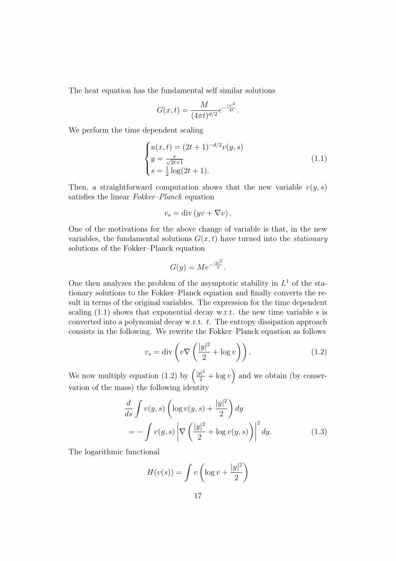
The heat equation has the fundamental self similar solutions

G(x, t) =M

(4πt)d/2e−

|x|24t .

We perform the time dependent scalingu(x, t) = (2t+ 1)−d/2v(y, s)

y = x√2t+1

s = 12log(2t+ 1).

(1.1)

Then, a straightforward computation shows that the new variable v(y, s)satisfies the linear Fokker–Planck equation

vs = div (yv +∇v) .

One of the motivations for the above change of variable is that, in the newvariables, the fundamental solutions G(x, t) have turned into the stationarysolutions of the Fokker–Planck equation

G(y) = Me−|y|22 .

One then analyzes the problem of the asymptotic stability in L1 of the sta-tionary solutions to the Fokker–Planck equation and finally converts the re-sult in terms of the original variables. The expression for the time dependentscaling (1.1) shows that exponential decay w.r.t. the new time variable s isconverted into a polynomial decay w.r.t. t. The entropy dissipation approachconsists in the following. We rewrite the Fokker–Planck equation as follows

vs = div

(v∇(|y|2

2+ log v

)). (1.2)

We now multiply equation (1.2) by(|y|22

+ log v)

and we obtain (by conser-

vation of the mass) the following identity

d

ds

∫v(y, s)

(log v(y, s) +

|y|2

2

)dy

= −∫v(y, s)

∣∣∣∣∇( |y|22+ log v(y, s)

)∣∣∣∣2 dy. (1.3)

The logarithmic functional

H(v(s)) =

∫v

(log v +

|y|2

2

)17

is called relative entropy (because of its evident relation with the classicalkinetic entropy functional). The Dirichlet type integral on the right handside of (1.3) is called Fisher information or entropy production. It is relatedto the relative entropy via the celebrated logarithmic Sobolev inequality (see[Gro75, AMTU01])∫

v(y, s)

(log v(y, s) +

|y|2

2

)dy

≤ 1

2

∫v(y, s)

∣∣∣∣∇( |y|22+ log v(y, s)

)∣∣∣∣2 dy. (1.4)

Hence, (1.4) and (1.3) yield the exponential decay for the relative entropy

d

ds

∫v(y, s)

(log v(y, s) +

|y|2

2

)dy

≤ e−2s

∫v(y, 0)

(log v(y, 0) +

|y|2

2

)dy. (1.5)

The following Csiszar–Kullback inequality

‖v(s)−G‖2L1 ≤ H(v(s))

provides then the exponential decay of the L1 difference between the solutionv and the gaussian equilibriumG with rate e−s, which in terms of the old vari-ables u(x, t) turns into an L1 polynomial decay towards the fundamental solu-tions with the optimal rate of t−1/2 (the optimality is immediately checked bytesting the relative entropy functional with shifted Gaussian kernels). This isdone by reasonable extra assumptions on the initial datum, namely L1 logL1

and finite second moment. The standard references for the above procedure,together with its generalizations to variable coefficient cases and the use ofalternative entropy functionals, are [AMTU00, AMTU01, MV00]. One im-portant remark is that, under few extra technical assumptions, the validityof a logarithmic Sobolev type inequality and the exponential decay in rela-tive entropy are equivalent. Hence, the use of different entropy functionalsyields to the proof of a huge variety of generalized Sobolev inequalities (thisequivalence is known as the Bakry–Emery point of view).

The above idea has been successfully generalized to nonlinear diffusionequations. In particular, the already mentioned results by Carrillo andToscani [CT00], Felix Otto [Ott01] and Del Pino and Dolbeault [DPD02a],allowed to obtain optimal rates of convergence in L1 for solutions to the PMEtowards Barenblatt profiles. These results hold also in cases of d−2

d< m < 1,

18

for which the nonlinear diffusion equation (1.1) is called fast diffusion equa-tion. After those results, a lot of generalization have been carried out for gen-eral parabolic equations and systems (see [CJM+01a]), p–laplacian equation(see [DPD02b]), convection–diffusion equations (see [CF03]), fourth–orderequations (see [CCT]).

The present thesis contains two contribution to this theory. The first oneconcerns with nonlinear diffusion equations of the form

ut = ∆φ(u),

where the function φ behaves like a power at the origin. In this case aresult was already present in the literature (namely [BDE02]). In Chapter5 we used an alternative entropy method in order to relax the hypothesison the nonlinearity present in [BDE02] in order to obtain the optimal rateof convergence towards Barenblatt profiles. The content of Chapter 5 is thesubject of a work in preparation of the author in collaboration with J. A.Carrillo and G. Toscani. In the next section we describe the second result inthis context, concerning with the one–dimensional viscous Burgers’ equation.

Finally, we remark that the entropy dissipation approach has been re-cently used outside of the context of diffusion equations. The first resultfor scalar conservation laws is due to Dolbeault and Escobedo in [DE]. Ourresult in Chapter 8 for the radiating gas model represents a new step in thisdirection.

1.8 The viscous Burgers’ equation

The simplest model describing both nonlinear convection and diffusive be-havior is the viscous Burgers’ equation

ut + uux = µuxx.

The study of this equation (introducted by Burgers in 1940), has been the keypoint for the development of the theory of shock waves and diffusion wavesfor viscous and non–viscous systems of conservation laws. A first detailedanalysis of this phenomena was performed by Hopf ([Hop50]) and succes-sively by Whitam ([Whi74]), who both constructed the typical intermediateasymptotic states for this equation (with summable initial data), namely, thediffusive N-waves and the nonnegative diffusive waves, and studied the trendtowards these profiles for solutions having initial datum in L1.

The study of the viscous Burgers’ equation is naturally related to that ofthe inviscid Burgers’ equation

ut + uux = 0. (1.1)

19

Indeed, it is well known that one of the most intuitive criterion for the se-lection of the unique entropy solution of the Cauchy problem for the inviscidcase is the µ→ 0 limit of the solutions of the viscous case.

At the stage of time–asymptotics, it is also well–known that the diffusionwaves of the viscous system are replaced by the N–waves (which are thepointwise limit of a diffusion wave as the viscosity tends to zero, in case ofpositive data) in the inviscid case (see the important paper by Tai Ping Liu[Liu85] and the paper by Liu and Pierre [LP84]). We refer to the introductionto [Liu85] for a clear explanation of the asymptotic stability of nonlinearwaves for viscous conservation laws.

This study is also related to the asymptotic self similar behavior for ageneral convection–diffusion equation. There are many important results onthis subject, see [EZ91, DZ92, Zua93, Zua94, EVZ93, EZ97, EZ99].

In Chapter 7, the long time asymptotics for the viscous Burgers’ equationis studied with the help of the entropy dissipation techniques described in theprevious section. In particular, the optimal rate of convergence in L1 towardsdiffusive waves is obtained. This was already known for this simple example(the solution is obtained via the Hopf Cole formula which turns the viscousBurgers’ equation into the linear heat equation). However, this is the firstcase where entropy dissipation has been employed to obtain optimal ratesof convergence to self–similarity for convection–diffusion equations (almostat the same time of [CF03] for the diffusion dominant cases). Moreover, itmust be remarked that the description of the evolution of such systems viathe entropy functionals is more significant from a thermodynamical point ofview than the classical Lp estimates. The results in Chapter 7 are containedinto the author’s paper [DFM] (joint work with Markowich).

1.9 The Wasserstein distance

The entropy dissipation machinery developed in the above mentioned papersis closely related to the so–called Wasserstein distance. This distance is de-fined on the space of probability measures with finite second moment andcomes as the minimal quadratic cost in the variational Monge–Kantorovichproblem of optimal mass tranportation (see [Vil03]). Its relation with theabove mentioned entropy functionals has been recently clarified by Felix Otto([Ott01]) in the context of gradient flows. More precisely, the porous mediumequation (and the linear heat equation as a special case) can be viewed asthe gradient flow of an entropy–type functional with respect to a Dirichletintegral type metric defined on the space of probability measures, which isendowed with a Riemannian structure. The Wasserstein metric comes as

20

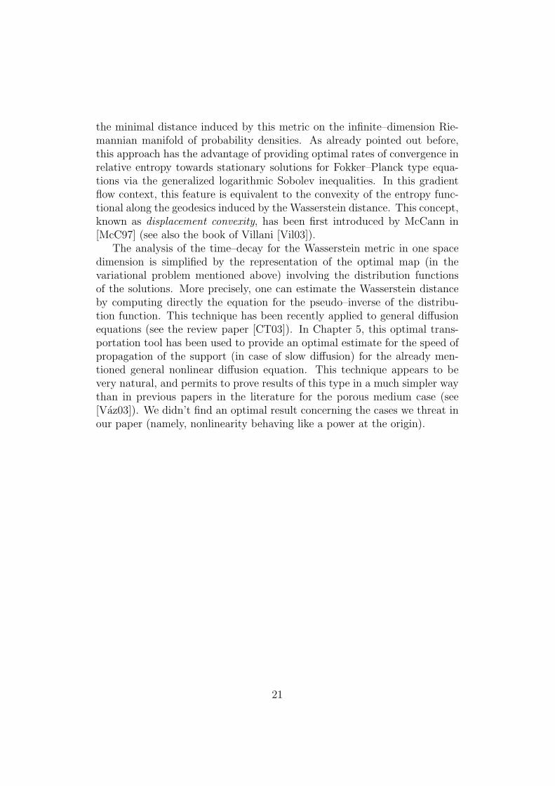
the minimal distance induced by this metric on the infinite–dimension Rie-mannian manifold of probability densities. As already pointed out before,this approach has the advantage of providing optimal rates of convergence inrelative entropy towards stationary solutions for Fokker–Planck type equa-tions via the generalized logarithmic Sobolev inequalities. In this gradientflow context, this feature is equivalent to the convexity of the entropy func-tional along the geodesics induced by the Wasserstein distance. This concept,known as displacement convexity, has been first introduced by McCann in[McC97] (see also the book of Villani [Vil03]).

The analysis of the time–decay for the Wasserstein metric in one spacedimension is simplified by the representation of the optimal map (in thevariational problem mentioned above) involving the distribution functionsof the solutions. More precisely, one can estimate the Wasserstein distanceby computing directly the equation for the pseudo–inverse of the distribu-tion function. This technique has been recently applied to general diffusionequations (see the review paper [CT03]). In Chapter 5, this optimal trans-portation tool has been used to provide an optimal estimate for the speed ofpropagation of the support (in case of slow diffusion) for the already men-tioned general nonlinear diffusion equation. This technique appears to bevery natural, and permits to prove results of this type in a much simpler waythan in previous papers in the literature for the porous medium case (see[Vaz03]). We didn’t find an optimal result concerning the cases we threat inour paper (namely, nonlinearity behaving like a power at the origin).

21

Part I

Relaxation limits

22

Chapter 2

The compressible Eulerequations with damping

In this chapter we will concern with a class of smooth solutions to the one-dimensional isentropic compressible Euler equations through porous mediaintroduced in section 1.3. As already pointed out in the introduction, af-ter a parabolic scaling we analyze the singular convergence towards caloricsolutions to the porous medium equation. The machinery developed hereholds far from vacuum, and it could be easily generalized to limiting profilessatisfying suitable decay estimates. In section 2.1 we describe the problemin details and we collect the main results in theorems 2.1.1 and 2.1.4. Theresult in 2.1.4 is closely related to the asymptotic stability result in chapter6. Section 2.2 is devoted to the proof of the main theorem 2.1.1.

2.1 Statement of the problem and results

Let us consider the one-dimensional, isentropic, compressible Euler equa-tions through a porous medium in eulerian coordinates. In case of smoothsolutions, with ρ > 0, the system may be written as∂τρ+ u∂xρ+ ρ∂xu = 0

∂τu+ u∂xu+p′(ρ)

ρ∂xρ = −u

ε.

(2.1.1)

Here, ρ > 0 is the density, u is the velocity, x ∈ R, τ > 0, p : R → R+ is asmooth function such that p′ > 0, and ε > 0 is a small parameter. After thetime scaling τ = t

ε, ρε(x, t) = ρ(x, t

ε), uε(x, t) = 1

εu(x, t

ε), the system (2.1.1)

23

becomes ∂tρε + uε∂xρ

ε + ρε∂xuε = 0

∂tuε + uε∂xu

ε +p′(ρε)

ε2ρε∂xρ

ε = −uε

ε2.

(2.1.2)

Thus, as ε goes to 0, we expect the solutions to (2.1.2) to be described bythe solutions to the following system

∂tρ+ ∂x(ρu) = 0

∂xp(ρ) = −ρu,(2.1.3)

which is equivalent to the Porous Medium equation

ρt = p(ρ)xx, (2.1.4)

where the relation between the pressure p and the velocity u is given by thewell known Darcy’s law

u = −p(ρ)xρ

. (2.1.5)

For the system (2.1.2), we prescribe the following limiting conditions at in-finity

ρε(±∞, t) = ρ± for any t ≥ 0

uε(±∞, 0) = u±,

with ρ+, ρ− > 0. Since we expect the inertial terms of the second equation in(2.1.2) to decay faster than the others, in addition we require

uε(±∞, t) = e−t/ε2

u± for any t ≥ 0.

Therefore, we assume the following behaviour at x → ±∞ for the system(2.1.3)

ρ(±∞, t) = ρ±

u(±∞, t) = 0,

for any t ≥ 0. The initial datum on the density of the hyperbolic problem(2.1.2) is assumed to be the same of (2.1.4), namely

ρε(x, 0) = ρ(x, 0) = ρ0(x),

where ρ0 is a bounded smooth function (e.g. ρ0 ∈ H3(R)) such that

0 < µ0 ≤ ρ0(x) ≤ µ1.

24

Moreover, we require the initial datum on the velocity uε to be given by theinitial value of u in the system (2.1.3) (which is determined by the Darcy’slaw) plus a small corrector, needed to match the limiting conditions, namely

uε0(x) = −p′(ρ0(x))

ρ0(x)ρ′0(x) + wε(x, 0). (2.1.6)

The expression for the corrector wε is

wε(x, t) = e−t/ε2

[u− + (u+ − u−)ψ(x)] , (2.1.7)

where

ψ(x) =

∫ x

−∞φ(y)dy∫ +∞

−∞φ(y)dy

,

for some φ ∈ C∞c (R), φ ≥ 0. We observe that wε satisfies the equation

∂twε = − 1

ε2wε.

This corrector doesn’t affect the asymptotic analysis since it decays expo-nentially fast. The well-prepared initial data condition (2.1.6) is prescribedin order to avoid the problem of the initial layer.

As a consequence of the boundedness of ρ0 and of the comparison principlefor the parabolic equation (2.1.4), we have

µ0 ≤ ρ(x, t) ≤ µ1. (2.1.8)

We will consider solutions (ρ, u) to (2.1.4) satisfying the time-asymptoticestimates ∣∣∣∣∂α+β ρ(t)

∂xα∂tβ

∣∣∣∣∞

=O(δ)1

(t+ 1)α2+β

α, β > 0∫ +∞

−∞

∣∣∣∣∂α+β ρ(x, t)

∂xα∂tβ

∣∣∣∣2dx =O(δ2)1

(t+ 1)α+2β− 12

α, β > 0 (2.1.9)∣∣∣∣∂α+βu(t)

∂xα∂tβ

∣∣∣∣∞

=O(δ)1

(t+ 1)α2+β+ 1

2

α, β ≥ 0∫ +∞

−∞

∣∣∣∣∂α+βu(x, t)

∂xα∂tβ

∣∣∣∣2dx =O(δ2)1

(t+ 1)α+2β+ 12

, α, β ≥ 0

whereδ = |ρ+ − ρ−|+ |u+ − u−|. (2.1.10)

25

In particular, these estimates are satisfied both by the caloric self-similarsolutions of (2.1.4) described in [HL92][Nis96] and by a small perturbationof these solutions w.r.t. initial datum (as we will show in the Theorem 6.1.1of Chapter 6).

Our first risult concerns the asymptotic behaviour as ε 0 of the scaledhyperbolic system (2.1.2) with Sobolev norms. The time interval where theasymptotic analysis is valid, is given by the condition εTα 1, for someconstant α > 0, which allows, for small ε, to include the solutions at largetime.

Theorem 2.1.1 Let 0 < ν < 1/2 be arbitrary. Suppose εT1+ν2 1, ε 1

and δ 1; then, there exists a fixed constant ∆ > 0 such that

sup0≤t≤T

1

(t+ 1)ν

[1

ε2‖ρε(t)− ρ(t)‖2

H3θ + ‖uε(t)− u(t)− wε(t)‖2H3θ+

1

ε2

∫ t

0

‖uε(s)− u(s)− wε(s)‖2H3θds

]≤ ∆, (2.1.11)

for any θ ∈ (0, 1).

Corollary 2.1.2 Let t > 0 be arbitrary. Let β > 0 be arbitrarily small.Then, for small values of δ, we have

‖ρε(t)− ρ(t)‖2L∞ + ‖ρεx(t)− ρx(t)‖2

L∞ ≤ O(ε2−β). (2.1.12)

Remark 2.1.3 Another simple consequence of Theorem 2.1.1 is the global–in–time existence of smooth solution for system (2.1.2) with fixed ε > 0 whenthe initial data are chosen to be small perturbations of the initial datum ofthe caloric profile ρ. This comes from Theorem 6.1.1 in Chapter 6 and fromthe continuation principle for quasi linear hyperbolic systems (see [Maj84]).

The proof of the Theorem (2.1.1) will be given in the Section 2.2. As aconsequence of the stability result in chapter 6, the result in Theorem 2.1.1 isalso true when the initial datum for ρ is replaced by a small perturbation ofthe initial datum of a caloric self similar profile. Moreover, as a consequenceof both Theorem 2.1.1 and Theorem 6.1.1 in chapter 6, we have the followingasymptotic result.

Theorem 2.1.4 Let ρ(x, t) be the caloric self-similar solution toρt = p(ρ)xx

ρ(x, 0) = ρ0(x)

ρ(±∞, t) = ρ±.

26

Let (ρε(x, t), uε(x, t)) be the solution to

ρεt + (ρεuε)x = 0

uεt + uεuεx +p(ρε)xε2ρε

= −uε

ε2

ρε(x, 0) = ρ0(x) = ρ(x+ x0) + r0(x)

uε(x, 0) = −p(ρ0(x))xρ0(x)

+ wε(x, 0)

ρε(±∞, t) = ρ±

uε(±∞, t) = e−t/ε2

u±,

with wε(x, t) given by (2.1.7), x0 given by (6.1.3). Suppose that ‖R(0)‖25, δ

and ε are sufficiently small (R(0) defined by (6.1.4)). Then, there exists afixed Γ > 0 such that

supγT (ε)≤t≤ΓT (ε)

‖ρε(t)− ρ(t)‖L∞(R) ≤ O(ε1

1+ν ), (2.1.13)

whereT (ε) = ε−

21+ν ,

ν > 0 is arbitrary small and γ is an arbitrary constant such that 0 < γ < Γ.

The proof of the theorem (2.1.4) is straightforward.

2.2 The Proof of the main Theorem

We prove Theorem 2.1.1 by means of an iteration scheme. Let us define anapproximating sequence (ρε(n), u

ε(n)) by setting,

ρε0 = ρ , uε0 = u+ wε,

and let, for any n > 1, (ρε(n), uε(n)) be the solution to the system

∂tρε(n) + ρε(n−1)∂xu

ε(n) + uε(n−1)∂xρ

ε(n) = 0

∂tuε(n) + uε(n−1)∂xu

ε(n) +

p′(ρε(n−1))

ε2ρε(n−1)

∂xρε(n) = −

uε(n)

ε2

ρε(n)(x, 0) = ρ0(x)

uε(n)(x, 0) = −p′(ρ0(x))

ρ0(x)ρ′0(x) + wε(x, 0)

ρε(n)(±∞, t) = ρ±

uε(n)(±∞, t) = e−t/ε2

u±.

(2.2.1)

27

We will prove the convergence of the approximating sequence (ρε(n), uε(n)) to

the solution of the system (2.1.2) via the uniform boundedness of this se-quence in some weighted high Sobolev norm (namely H3(R)) and the con-traction in some weighted L2-norm. Thus, we obtain the desired estimatevia interpolation. This strategy is used in [KM81][KM82][Maj84].

Denote, for any T > 0,

Enε (T ) = sup0≤t≤T

1

(t+ 1)ν

[1

ε2‖(ρε(n) − ρ)(t)‖2

H3+

+‖(uε(n) − u− wε)(t)‖2H3 +

1

ε2

∫ t

0

‖(uε(n) − u− wε)(s)‖2H3ds

]. (2.2.2)

Hence, we have the following result

Proposition 2.2.1 Let us suppose that δ + ε + εT1+ν2 ≤ λ, where λ 1.

Then, there exists a positive constant ∆ > 0 such that, for any n ∈ N,

Enε (T ) ≤ ∆. (2.2.3)

Proof. From now on, we denote

ρ = ρε(n) u = uε(n) ρ = ρε(n−1) u = uε(n−1)

ρ = ρ− ρ u = u− wε − u ρ = ρε(n−2)u = uε(n−2)

¯ρ = ρ− ρ ¯u = u− wε − u ¯u = u− u− w π(z) = p′(z)z, for anyz ∈ R+.

The system (2.2.1) becomes

ρt + uρx + ρux =− (¯u+ w)ρx − ¯ρux − ρwx (2.2.4)

ut + uux +1

ε2π(ρ)ρx =−ut−u(ux+wx)−

1

ε2(π(ρ)−π(ρ))ρx−

u

ε2. (2.2.5)

We now assume that the estimate (2.2.3) holds for (ρ, u) and show that it istrue for (ρ, u). In particular, we assume

sup0≤t≤T

1

(t+1)ν

[1

ε2‖ ¯ρ(t)‖2

H3+‖¯u(t)‖2H3+

1

ε2

∫ t

0

‖¯u(s)‖2H3ds ≤ ∆

], (2.2.6)

for any T > 0, ε > 0 and δ > 0 (δ defined by (2.1.10)) such that

δ + ε+ εT1+ν2 ≤ λ , λ 1. (2.2.7)

As usual in this framework, we determine the conditions on the constant∆ in the estimate at the n−th step. As we will see, this constant depends

28

only on the constant λ in (2.2.7). Let us multiply (2.2.4) by (1/ε2)π(ρ)ρand (2.2.5) by ρu. Then, via standard energy identity (as a consequence ofsymmetrization), we get

d

dt

∫ +∞

−∞

[1

ε2π(ρ)

ρ2

2+ ρ

u2

2

]dx =

=

∫ +∞

−∞(π′(ρ)(ρt + ρxu)+π(ρ)ux)

ρ2

2ε2dx+

∫ +∞

−∞(ρt + ρxu+ ρux)

u2

2dx+

+

∫ +∞

−∞

1

ε2p′′(ρ)ρxρudx−

∫ +∞

−∞

1

ε2π(ρ)ρ(¯u+w)ρxdx−

∫ +∞

−∞

1

ε2π(ρ)ρ ¯ρuxdx+

−∫ +∞

−∞

1

ε2π(ρ)ρρwxdx−

∫ +∞

−∞ρutudx−

∫ +∞

−∞ρuu(ux + wx)dx+

−∫ +∞

−∞

1

ε2ρu(π(ρ)− π(ρ))ρxdx−

∫ +∞

−∞ρu2

ε2dx =

=:3∑

k=1

Jk(t) +6∑

k=1

Ik(t)−∫ +∞

−∞ρu2

ε2dx. (2.2.8)

Remark 2.2.2 We remark that the function π(z) satisfies

0 < c0 ≤ π(z) ≤ c1, as z ∈ (c2, c3),

for some positive constants c0, c1, c2, c3. Now, from the assumption (2.2.6)and from (2.1.8), it follows that ρ satisfies

0 <µ0

2≤ ρ(x, t) ≤ µ1 +

µ0

2, for any x ∈ R, 0 ≤ t ≤ T. (2.2.9)

(where µ0, µ1 are defined in (2.1.8)) provided that

ε(T + 1)ν/2 ≤ ∆−1/2µ0

2,

(with ∆ as in (2.2.6)). Thus, from the condition (2.2.7) and by requiring

∆ < 1 and λν

1+ν ε1

1+ν < µ0

2(i.e. ε + λ 1), there exist C1, C2 fixed positive

constants such thatC1 ≤ π(ρ) ≤ C2. (2.2.10)

Moreover, from (2.2.9) it follows that

π′(ρ) + p′′(ρ) ≤ C3, (2.2.11)

for some positive fixed C3.

29

Now, from (2.2.9), (2.2.10), (2.2.11), and after time integration of (2.2.8) in[0, t], for 0 < t ≤ T , T satisfying (2.2.7), it follows that

1

ε2‖ρ(t)‖2 + ‖u(t)‖2 +

1

ε2

∫ t

0

‖u(s)‖2ds ≤

≤O(1)

∫ t

0

[|ρt|∞ + |ρxu|∞ + |ux|∞]

[‖ρ(s)‖2

ε2+ ‖u(s)‖2

]ds+

+O(1)

ε2

∫ t

0

|ρx|∞‖ρ(s)‖‖u(s)‖ds+

∫ t

0

6∑k=1

Ik(s)ds =

=:2∑

h=1

Jh(t) +6∑

k=1

∫ t

0

Ik(s)ds. (2.2.12)

We devote ourselves to the estimate of the terms∫ t

0Ik(t)ds, k = 1, . . . 6.

In what follows, we exploit (2.2.6), (2.2.7), the time asymptotic estimates(2.1.9) and the estimates (2.1.8), (2.2.10), (2.2.11).∫ t

0

I1ds ≤O(δ)

ε2

∫ t

0

‖¯u(s)‖‖ρ(s)‖ 1

(s+ 1)1/2ds+

+O(1)

ε2

∫ t

0

e−s

ε2 ‖ρ(s)‖‖ρx(s)‖ds ≤

≤O(δ)

ε2

∫ t

0

‖¯u‖2ds+O(δ)

ε2

∫ t

0

‖ρ(s)‖2

s+ 1ds+

+O(1)

ε2

∫ t

0

e−s

ε2[‖ρ(s)‖2 + ‖ρx(s)‖2

]ds ≤

≤O(δ)

(∆(t+ 1)ν +

∫ t

0

En(s)(s+ 1)1−ν ds+ 1

)+ En(t)(t+ 1)νε2 ≤

≤O(δ) (∆(t+ 1)ν + 1) + En(t)(t+ 1)ν(O(δ) +O(ε2)). (2.2.13)

∫ t

0

I2ds ≤O(δ)

ε2

∫ t

0

‖ρ(s)‖‖ ¯ρ(s)‖ 1

s+ 1ds ≤

≤O(δ)

ε2

∫ t

0

[‖ρ(s)‖2 + ‖ ¯ρ(s)‖2

] 1

s+ 1ds ≤

≤O(δ)

∫ t

0

En(s)(s+ 1)1−ν ds+O(δ)

∫ t

0

∆1

(s+ 1)1−ν ds ≤

≤O(δ)En(t)(t+ 1)ν +O(δ)∆(t+ 1)ν . (2.2.14)

30

∫ t

0

I3ds =

∫ t

0

∫ +∞

−∞

π(ρ)

ε2ρ ¯ρwxdxds+

∫ t

0

∫ +∞

−∞

π(ρ)

ε2ρρwxdxds ≤

≤O(δ)

ε2

∫ t

0

‖ρ(s)‖‖ ¯ρ(s)‖e−s

ε2 ds+O(δ)

ε2

∫ t

0

∫supp(φ)

ρe−s

ε2 dxds ≤

≤O(δ)En(t)(t+ 1)ν +O(δ)∆(t+ 1)ν +O(δ)

ε2

∫ t

0

|ρ|∞e−s

ε2 ds ≤

≤O(δ) + En(t)O(δ)(1 + (t+ 1)ν) +O(δ)∆(t+ 1)ν ,

where in the second inequality we have used the estimate for∫ t

0I2.∫ t

0

I4ds ≤ O(1)

∫ t

0

[‖ut(s)‖2 + ‖u(s)‖2

]ds ≤

≤O(δ2)

∫ t

0

1

(s+ 1)5/2ds+O(ε2)En(t)(t+ 1)ν ≤

≤O(δ2) +O(ε2)En(t)(t+ 1)ν .

∫ t

0

I5ds ≤∫ t

0

∫ +∞

−∞¯uρu(ux+wx)dxds+

∫ t

0

∫ +∞

−∞(u+ w)(ux+ wx)ρudxds≤

≤O(1)

∫ t

0

[‖¯u(s)‖2 + ‖u(s)‖2

]ds+O(1)

∫ t

0

[‖ux(s)‖2 + ‖u(s)‖2

]ds+

+O(1)

∫ t

0

[‖wx(s)‖2 + ‖u(s)‖2

]ds ≤

≤O(ε2)(∆(t+1)ν+En(t)(t+1)ν+O(δ2)

)+O(δ2)

∫ t

0

1

(s+ 1)3/2ds≤

≤O(δ2) +O(ε2)(∆(t+ 1)ν + En(t)(t+ 1)ν +O(δ2)

).

∫ t

0

I6ds ≤O(δ)

ε2

∫ t

0

‖ ¯ρ(s)‖‖u(s)‖ 1

(s+ 1)1/2ds ≤

≤O(δ)

ε2

∫ t

0

‖ ¯ρ(s)‖2 1

s+ 1ds+

O(δ)

ε2

∫ t

0

‖u(s)‖2ds ≤

≤O(δ)(t+ 1)ν (∆ + En(t)) .

Thus, by requiring ∆ < 1 and λ 1, the estimates of these terms yields

6∑k=1

∫ t

0

Ik(t) ≤ O(λ) (∆ + En(t)) (t+ 1)ν +O(λ)(t+ 1)ν .

31

Hence, we compute the integrals denoted by Jh, h = 1, 2.

J1(t) ≤ O(1)

∫ t

0

[|ρ(s)|∞|ux(s)|∞ + |u(s)|∞|ρx(s)|∞+

+ |ρx(s)|∞|u(s)|∞ + |ux(s)|∞] [‖ρ(s)‖2

ε2+ ‖u(s)‖2

]ds ≤

≤O(1)

∫ t

0

[|ux(s)|∞+|ρx(s)|∞

(|u(s)|∞+ |u(s)|∞)][‖ρ(s)‖2

ε2+‖u(s)‖2

]ds ≤

≤O(1)En(t)∫ t

0

[|ux(s)|∞+|ρx(s)|∞

(|u(s)|∞+ |u(s)|∞)] (s+ 1)νds ≤

≤O(1)En(t)∫ t

0

[|¯ux(s)|∞+|ux(s)|∞+|wx(s)|∞+ (| ¯ρx(s)|∞+|ρx(s)|∞) ·

·(|¯u(s)|∞ + | ¯u(s)|∞ + |u(s)|∞ + |w(s)|∞

)](s+ 1)νds. (2.2.15)

We now estimate separately the following terms.∫ t

0

|¯ux(s)|∞(s+ 1)νds ≤∫ t

0

(λ|¯ux(s)|2∞

ε2+

1

λε2(s+ 1)2ν

)ds ≤

≤λ∆(t+ 1)ν+1

λε2(t+ 1)1+2ν ≤ O(λ)(t+ 1)ν (2.2.16)

where λ is the fixed constant in (2.2.7).∫ t

0

(| ¯ρx(s)|∞+|ρx(s)|∞)(|¯u(s)|∞ + | ¯u(s)|∞

)(s+ 1)νds ≤

≤∫ t

0

(ε∆1/2(s+ 1)

3ν2 +O(δ)(s+ 1)−1/2+ν

) (|¯u(s)|∞ + | ¯u(s)|∞

)≤

≤(O(λ)+O(δ))

∫ t

0

(|¯u(s)|∞ + | ¯u(s)|∞

)≤ (O(λ) +O(δ))(t+ 1)ν (2.2.17)

where the last inequality is justified by the preceding estimate (2.2.16), andwhere we used ν < 1/2 and ∆ < 1.∫ t

0

(| ¯ρx(s)|∞+|ρx(s)|∞) (|u(s)|∞ + |w(s)|∞) (s+ 1)νds ≤

≤∫ t

0

(ε∆1/2(s+ 1)

3ν2 +O(δ)(s+ 1)−1/2+ν

)O(δ)(s+ 1)−1/2ds+

+O(ε)∆1/2(t+ 1)ν/2 +O(δ)O(ε2) ≤ (O(λ) +O(δ))(t+ 1)ν . (2.2.18)

32

Now we can complete the estimate of the integral J1 in (2.2.15), and obtain

J1(t) ≤(O(δ) +O(λ) +O(ε2)

)(t+ 1)νEn(t).

Let us estimate J2(t);

J2(t) ≤ O(1)

∫ t

0

[| ¯ρx(s)|∞ + |ρx(s)|∞]1

ε2‖ρ(s)‖‖u(s)‖ds ≤

≤O(1)

∫ t

0

[ε∆1/2(s+ 1)ν/2 +O(δ)(s+ 1)−1/2

] 1

ε2‖ρ(s)‖‖u(s)‖ds ≤

≤O(1)ε∆1/2

∫ t

0

[‖ρ(s)‖2

λε(s+ 1)ν + λ

‖u(s)‖2

ε3

]ds+

+O(δ)

∫ t

0

‖ρ(s)‖2

ε2(s+ 1)−1ds+O(δ)

∫ t

0

‖u(s)‖2

ε2ds ≤

≤O(1)ε2

λ(t+ 1)1+2νEn(t) + (O(λ) +O(δ)) En(t)(t+ 1)ν . (2.2.19)

By combining all these estimates, dividing both sides of (2.2.12) by (t+ 1)ν ,taking the sup0≤t≤T and by suitably choosing ∆ and λ such that

0 < ∆ < 1, ∆ > Cλ,

for a fixed constant C, we obtain the following

Lemma 2.2.3 Suppose δ+ε+εT1+ν2 ≤ λ 1. Then, there exists a positive

fixed constant ∆ such that

sup0≤t≤T

1

(1 + t)ν

[1

ε2‖ρ(t)‖2 + ‖u(t)‖2 +

1

ε2

∫ t

0

‖u(s)‖2ds

]≤ ∆

4, (2.2.20)

In a similar fashion, we can derive L2 estimates for the derivatives of ρand u. By differentiatiting (2.2.4)-(2.2.5) w.r.t. x, we obtain

ρxt + uρxx + ρuxx =−uxρx−ρxux−(¯ux+wx)ρx−(¯u+w)ρxx+

− ¯ρxux − ¯ρuxx − ρxwx − ρwxx, (2.2.21)

uxt + uuxx +1

ε2π(ρ)ρxx =− uxux−

1

ε2π′(ρ)ρxρx − uxt − ux(ux+wx)+

− u(uxx + wxx)−1

ε2(π(ρ)− π(ρ)) ρxx+

− 1

ε2(π′(ρ)ρx − π′(ρ)ρx) ρx −

1

ε2ux. (2.2.22)

33

It is clear that the system (2.2.21)-(2.2.22) has the same stucture as system(2.2.4)-(2.2.5). Thus, by multiplying the first equation by 1

ε2π(ρ)ρx and the

second equation by ρux, we obtain an energy identity similar to (2.2.8). Then,by integrating w.r.t. time, and from the same considerations as those in theremark 2.2.2, we obtain

1

ε2‖ρx(t)‖2 + ‖ux(t)‖2 +

1

ε2

∫ t

0

‖ux(s)‖2ds ≤

≤O(1)

∫ t

0

[|ρt|∞ + |ρxu|∞ + |ux|∞]

[‖ρx(s)‖2

ε2+ ‖ux(s)‖2

]ds+

+O(1)

ε2

∫ t

0

|ρx|∞‖ρx(s)‖‖ux(s)‖ds+

∫ t

0

G(s)ds+

∫ t

0

F (s)ds,

where we denoted all the integrals involving ρ, u and w by∫ t

0F (s)ds, and

where∫ t

0

G(s)ds =O(1)

ε2

∫ t

0

∫ +∞

−∞uxρ

2xdxds+

O(1)

ε2

∫ t

0

∫ +∞

−∞ρxuxρxdxds+

+O(1)

∫ t

0

∫ +∞

−∞uxu

2xdxds. (2.2.23)

The terms (2.2.23) are to be treated as the terms∑2

h=1 Jh of the previous

lemma. The integrals denoted by∫ t

0F (s)ds are made up by bilinear terms (in

the variables marked by and ), where the terms estimated in L∞ dependsonly on the corrector w and on the derivatives of asymptotic profile ρ, as inthe estimates of the integrals

∫ t0Ik(s) of the previous lemma (we also have a

faster decay for these terms, which involve second order derivatives). Hence,we easily obtain the following

Lemma 2.2.4 Suppose δ+ε+εT1+ν2 ≤ λ 1. Then, there exists a positive

fixed constant ∆ such that

sup0≤t≤T

1

(1 + t)ν

[1

ε2‖ρx(t)‖2 + ‖ux(t)‖2

+1

ε2

∫ t

0

‖ux(s)‖2ds

]≤ ∆

4, (2.2.24)

Remark 2.2.5 To complete the proof of the theorem 2.1.1, we differentiatew.r.t. x in order to get estimates for second and third derivatives of (ρ, u).The analogous of terms (2.2.23) behave the same as above (there is always acoefficient with order of derivation less then or equal to 2, to be estimated in

34

L∞(R)). Since these computations are very similar to those concerning thepreceding L2 estimates, we skip the details about them. Hence, the proof ofthe proposition is complete.

We now prove the contraction of the sequence (ρε(n), uε(n)) in the following

Proposition 2.2.6 Let us denote, for any ε > 0, n ∈ N, 0 < ν < 1/2,

Fnε (T )= sup

0≤t≤T

1

(t+1)ν

[1

ε2‖ρε(n)(t)−ρε(n−1)(t)‖2

L2+‖uε(n)(t)−uε(n−1)(t)‖2

L2+

+1

ε2

∫ t

0

‖uε(n)(s)− uε(n−1)(s)‖2L2ds

].

Then, under the condition δ + ε + εT1+ν2 ≤ λ, for λ 1, there exists a

positive constant µ < 1 such that

Fnε (T ) ≤ µFn−1

ε (T ). (2.2.25)

Proof. We denote

ρε(n−2) = ρ ρε(n−1) = ρ ρε(n) = ρ

uε(n−2) = u uε(n−1) = u uε(n) = u

ρ = ρ− ρ ¯ρ = ρ− ρ u = u− u ¯u = u− u.With this notation, we can write system (2.2.1) asρt + ρux + uρx = − ¯ρux − ¯uρx

ut + uux +1

ε2π(ρ)ρx = −¯uux −

(1

ε2π(ρ)− 1

ε2π(ρ)) ρx − u

ε2.

(2.2.26)

As in the preceding proposition, we symmetrize the system (2.2.26) by[1ε2π(ρ) 0

0 ρ

]

35

and obtain the standard enegy identity

d

dt

∫ +∞

−∞

[p′(ρ)

ε2ρ

ρ2

2+ ρ

u2

2

]dx =

=

∫ +∞

−∞

[(π′(ρ)(ρt + ρxu) + π(ρ)ux)

ρ2

2ε2

]dx+

+

∫ +∞

−∞

[(ρt + ρxu+ ρux)

u2

2+

1

ε2p′′(ρ)ρxρu

]dx+

−∫ +∞

−∞π(ρ)ρ¯uρxdx−

∫ +∞

−∞π(ρ)ρ ¯ρuxdx+

−∫ +∞

−∞ρu¯uuxdx−

∫ +∞

−∞ρu(π(ρ)− π(ρ))ρxdx− ∫ +∞

−∞ρu2

εdx. (2.2.27)

As a consequence of the proposition (2.2.1), after some considerations aboutthe symmetrizing coefficients (same as those in the remark 2.2.2), we obtainthe same estimates as (2.2.9), (2.2.10), (2.2.11), under the condition (2.2.7).After time integration in the interval [0, t] for 0 < t < T , we obtain

1

ε2‖ρ(t)‖2 + ‖u(t)‖2 +

1

ε2

∫ t

0

‖u(s)‖2ds ≤

≤O(1)

∫ t

0

[|ρt|∞ + |ρxu|∞ + |ux|∞]

[‖ρ(s)‖2

ε2+ ‖u(s)‖2

]ds+

+O(1)

ε2

∫ t

0

|ρx|∞‖ρ(s)‖‖u(s)‖ds+O(1)

ε2

∫ t

0

∫ +∞

−∞ρ ¯ρuxdxds+

+O(1)

ε2

∫ t

0

∫ +∞

−∞ρ¯uρx +O(1)

∫ t

0

∫ +∞

−∞¯uuxudxds+

O(1)

ε2

∫ t

0

∫ +∞

−∞¯ρuρxdxds =

=6∑

k=1

Lk(t).

We now consider each term separately, using the result of the proposition(2.2.1).

L1(t) ≤O(1)Fn(t)

∫ t

0

[|ρx(s)|∞

(|u(s)|∞+|u(s)|∞

)+|ux(s)|∞

](s+ 1)νds≤

≤O(1)Fn(t)

∫ t

0

[|(u− u− w)x(s)|∞+|ux(s)|∞+|wx(s)|∞+

+(|(ρ− ρ)x(s)|∞+|ρx(s)|∞

)(|(u− u− w)(s)|∞+

+ |(u− u− w)(s)|∞ + |u(s)|∞ + |w(s)|∞)]

(s+ 1)νds.

36

We estimate this term as in (2.2.16), (2.2.17), (2.2.18) of the proposition(2.2.1) and obtain

L1(t) ≤(O(δ) +O(λ) +O(ε2)

)(t+ 1)νFn(t).

Then, in a similar fashion, we estimate the term L2(t) as in (2.2.19). Let uscompute the remaining terms;

L3(t) ≤O(1)

ε2

∫ t

0

|ux(s)|∞‖ρ(s)‖‖ ¯ρ(s)‖ds ≤

≤O(1)

ε2

∫ t

0

[‖ρ(s)‖2

(s+ 1)ν+‖ ¯ρ(s)‖2

(s+ 1)ν

]|ux(s)|∞(s+ 1)νds ≤

≤O(1)[Fn(t)+Fn−1(t)

] ∫ t

0

[λ|(u− u− w)x|2∞

ε2+ε2(s+1)2ν

λ+

+O(δ)(s+1)ν−1

]ds≤ [O(λ) +O(δ)] (t+ 1)ν

(Fn(t) + Fn−1(t)

),

where we have used the condition (2.2.7).

L4(t) ≤O(1)

ε2

∫ t

0

|ρx(s)|∞‖ρ(s)‖‖¯u(s)‖ds ≤

≤O(1)

∫ t

0

[λ‖¯u(s)‖2

ε2+|ρx(s)|2∞‖ρ(s)‖2

λε2(s+ 1)ν(s+ 1)ν

]ds ≤

≤O(λ)Fn−1(t)(t+ 1)ν+O(1)1

λFn(t)

∫ t

0

[|(ρ− ρ)x(s)|2∞(s+ 1)ν+

+ O(δ)(s+ 1)ν−1]ds ≤

≤ [O(λ) +O(δ)] (t+ 1)ν(Fn(t) + Fn−1(t)

).

The integrals L5(t) and L6(t) can be treated as above. Thus, by suitablychoosing δ and λ small, the proof is complete.

We finally arrive to the convergence of the approximating sequence. Letν, ε and T be fixed in the usual way. Since (ρnε , u

nε ) is a Cauchy sequence in

the norm expressed by Fn, by interpolation we have

sup0≤t≤T

1

(t+ 1)ν

[1

ε2‖(ρε(n) − ρε(m))(t)‖2

H3θ + ‖(uε(n) − uε(m))(t)‖2H3θ+

+1

ε2

∫ t

0

‖(uε(n) − uε(m))(t)‖2H3θds

]→ 0 as n,m→∞. (2.2.28)

37

for any θ ∈ (0, 1). Thus, the approximating sequence (ρnε , unε ) converges in

the norm expressed by (2.2.28) to (ρ∗, u∗). By choosing θ ∈ (0, 1) big enough,we obtain

(ρnε , unε ) → (ρ∗, u∗) in L∞([0, T ];H2(R)). (2.2.29)

Hence, we can identify the limit as the solution (ρε, uε) to the system (2.1.2)and carry out the limit as n→∞ in the estimate (2.2.3), with H3θ in placeof H3, and the proof of the theorem (2.1.1) is complete.

38

Chapter 3

A one dimensional model forviscoelasticity

The present chapter is devoted to the study of the diffusive relaxation modelfor viscoelasticity described in section 1.4. The next section 3.1 contains thefirst rigorous justification of the relaxation scheme in theorem 3.1.1, which isproved via standard symmetrization and compactness arguments. In section3.2 we provide a rate of convergence in L2 norm. Finally, in section 3.3 weprove a result concerning travelling waves for the model considered.

3.1 Global existence and singular convergen-

ce of H1 solutions

In this section we study the global existence of H1 solutions and the relax-ation limit for the nonhomogeneous strictly hyperbolic system

ut − vx = 0

vt − zx = 0

ε2zt − µvx = −z + σ(u),

(3.1.1)

where (x, t) ∈ R×R+ are the independent variables, u, v and z take values inR, µ is a positive constant, ε > 0 is the relaxation parameter and σ : R → Ris a smooth function. We rewrite the semilinear system (3.1.1) as follows

Wt +AεWx = Qε(W ), (3.1.2)

where

W =

uvz

Aε(W ) =

0 −1 00 0 −10 − µ

ε20

Qε(W ) =1

ε2

00

−z + σ(u)

.

39

We recall that, for system (3.1.2) with fixed ε and µ, a local existence re-sult holds. More precisely, if the initial datum (u(·, 0), v(·, 0), z(·, 0)) be-longs in L∞(R), then there exists a positive time T such that the solution(u(t), v(t), z(t)) exists in L∞(R) for t ∈ [0, T ]. Since the matrix Aε is con-stant, the solution to (3.1.1) is global in time once the following estimate isverified

limt↑T ∗

[‖u(·, t)‖L∞(R) + ‖v(·, t)‖L∞(R) + ‖z(·, t)‖L∞(R)

]< +∞, (3.1.3)

where [0, T ∗] is the maximal time interval of existence of the solution. Theestimate (3.1.3) and the global existence of solutions to (3.1.1) for ε > 0 fixedare well known, provided that the following globally Lipschitz condition onthe function σ holds

supu∈R

|σ′(u)| < +∞. (3.1.4)

However, we shall obtain this a priori L∞ bound, which guarantees the globalexistence of solutions, as a consequence of the following theorem, which ac-tually provides a stronger estimate, namely an estimate for the H1–normof the solutions, with initial datum (u(·, 0), v(·, 0), z(·, 0)) ∈ H1(R), uniformwith respect to the parameter ε.

Theorem 3.1.1 Let (u, v, z)(·, t) be the solution to the system (3.1.1) withinitial data (u, v, z)(·, 0) ∈ H1(R). Suppose that the function σ satisfies con-dition (3.1.4). Then, the following inequality holds for any t > 0

ε2‖z(t)‖2H1(R) + ‖u(t)‖2

H1(R) + ‖v(t)‖2H1(R) +

∫ t

0

‖z(s)‖2H1(R)ds

≤[ε2‖z(0)‖2

H1(R) + ‖u(0)‖2H1(R) + ‖v(0)‖2

H1(R)

]eCt, (3.1.5)

where C is a positive constant depending only on supu∈R

|σ′(u)|.

Proof. We prove estimate (3.1.5) by means of energy estimates. To thisaim, we employ that system (3.1.1) admits a symmetrizer, which is positivedefinite for small values of ε, namely

Bε =

µε2

0 −10 µ

ε2− 1 0

−1 0 1

.

Hence, we define the energy

Eε (W ) = (BεW,W )L2(R) =

∫ +∞

−∞

[ µε2u2 − 2uz +

( µε2− 1)v2 + z2

]dx

40

and we observe that, for ε2 ≤ µ3,

Eε (W ) ≥ 1

2

∫ +∞

−∞

[ µε2u2 +

µ

ε2v2 + z2

]dx. (3.1.6)

Thus, (3.1.2) and integration by parts yields

d

dtEε (W (t)) = −2

∫ +∞

−∞BεAεWxWdx+ 2

∫ +∞

−∞BεQε (W )Wdx

= 2

∫ +∞

−∞BεQε (W )Wdx.

After integration over the time interval [0, t], we get

Eε (W (t))− Eε (W (0)) = 2

∫ t

0

∫ +∞

−∞BεQε (W (s))W (s)dxds =: I (W ) .

(3.1.7)We now estimate the term I (W ) in (3.1.7) as follows

I (W ) =2

ε2

∫ t

0

∫ +∞

−∞

[zu− uσ(u)− z2 + zσ(u)

]dxds

≤ − 1

ε2

∫ t

0

‖z(s)‖2L2(R)ds+

3

ε2

∫ t

0

[‖u(s)‖2

L2(R)

+

∫ +∞

−∞|σ(u(x, s))|2dx

]ds

≤ − 1

ε2

∫ t

0

‖z(s)‖2L2(R)ds+

3

ε2

(1 + sup

u|σ′(u)|2

)∫ t

0

‖u(s)‖2L2(R)ds,

if we assume, without loss of generality, σ(0) = 0. Thus, combining (3.1.7)and (3.1.6) one has

ε2‖z(t)‖2L2(R) + ‖u(t)‖2

L2(R) + ‖v(t)‖2L2(R) +

∫ t

0

‖z(s)‖2L2(R)ds

≤ C1

(ε2‖z(0)‖2

L2(R) + ‖u(0)‖2L2(R) + ‖v(0)‖2

L2(R)

)+ C2

∫ t

0

‖u(s)‖2L2(R)ds,

(3.1.8)

where C1 and C2 are fixed positive constant with C2 depending on σ′. We nowperform a similar estimate for the spatial derivative Wx. By differentiating(3.1.2) with respect to x, we get

Wxt +AεWxx = Qε(W )x,

41

Thus, proceeding as before, we get

Eε (Wx(t))− Eε (Wx(0)) = 2

∫ t

0

∫ +∞

−∞BεQε (W (s))xWx(s)dxds =: J (Wx) .

(3.1.9)We estimate the integral term J (Wx) as follows

J (Wx) =2

ε2

∫ t

0

∫ +∞

−∞BεQε (W )xWxdxds

=2

ε2

∫ t

0

∫ +∞

−∞

[−z2

x − σ′(u)u2x + (σ′(u) + 1)uxzx

]dxds

≤ − 1

2ε2

∫ t

0

‖zx(s)‖2L2(R)ds+ C3

∫ t

0

‖ux(s)‖2L2(R)ds, (3.1.10)

with C3 depending only on σ′, as in the previous estimate. From (3.1.6),(3.1.9) and (3.1.10), we get

ε2‖zx(t)‖2L2(R) + ‖ux(t)‖2

L2(R) + ‖vx(t)‖2L2(R) +

∫ t

0

‖zx(s)‖2L2(R)ds

≤ C4

(ε2‖zx(0)‖2

L2(R) + ‖ux(0)‖2L2(R) + ‖vx(0)‖2

L2(R)

)+ C5

∫ t

0

‖ux(s)‖2L2(R)ds, (3.1.11)

with C4 and C5 positive constants, C5 depending on σ′. Thus, from (3.1.8),(3.1.11) and from the Gronwall Lemma, we recover the estimate (3.1.5) andthe proof is complete.

The following estimates for the time derivatives of u, v and z are animmediate consequence of (3.1.5)

‖ut(t)‖2L2(R) +

∫ t

0

‖vt(s)‖2L2(R)ds ≤ KeCt, (3.1.12)∫ t

0

‖εzt(s)‖2L2(R)ds ≤ KeCt,

with K positive constant depending on the initial datum. In particular,(3.1.5) and (3.1.12) imply that the solution (u, v, z) verifies u ∈ H1([0, T ]×R),v ∈ H1([0, T ] × R) and εz ∈ H1([0, T ] × R). Hence, as a first consequenceof the above estimates, we have obtained the well known relation (3.1.3),and thus the global existence of solutions to (3.1.1) in L∞, for ε > 0 fixed.Moreover, since our estimates are uniform in ε, we can prove a first result ofconvergence for our semilinear relaxation approximation.

42

Corollary 3.1.2 Let (uε, vε, zε)(·, t) be the solution to the system (3.1.1)with initial data (u, v, z)(·, 0) ∈ H1(R). Suppose that the function σ satisfiescondition (3.1.4). Then,

uε → u, strongly in Lploc([0, T ]× R), 2 ≤ p < +∞,

vε → v, strongly in Lploc([0, T ]× R), 2 ≤ p < +∞,

and (u, v) is the solution ofut − vx = 0

vt − σ(u)x = µvxx

with (u0, v0) as initial condition.

Proof. Since estimates (3.1.5) and (3.1.12) are uniform in ε, the family ofsolutions uε, vε, zεε>0 to system (3.1.1) satisfies the following properties,for any T > 0,

uε uniformly bounded in H1([0, T ]× R), (3.1.13)

vε uniformly bounded in H1([0, T ]× R), (3.1.14)

zε uniformly bounded in L2([0, T ];H1(R)). (3.1.15)

Hence, from (3.1.13) and (3.1.14) we deduce that the sequence uε and vεis compact in Lploc([0, T ] × R) for any 2 ≤ p < +∞. Therefore, as ε ↓ 0, weobtain, passing if necessary to subsequences,

uε → u, vε → v, strongly in Lploc([0, T ]× R), 2 ≤ p < +∞.

Finally, by taking advantage of (3.1.15), we pass in the limit as ε ↓ 0 intosystem (3.1.1) with initial datum (u0, v0, z0) ∈ H1(R), and we recover thatthe limit functions u and v satisfy

ut − vx = 0

vt − σ(u)x = µvxx

u(·, 0) = u0

v(·, 0) = v0

(3.1.16)

in distributional sense.Now, for any T > 0, the initial value problem (3.1.16) admits a unique

solution (u, v) ∈ L∞([0, T ], H1(R)) (see Appendix A). Therefore, all thesequence (uε, vε) converges to (u, v) strongly in Lploc, for any 2 ≤ p < +∞and the proof is complete.

43

3.2 Rate of convergence in L2 norm

In the previous section we proved the strong convergence of H1 solutionsof the semilinear relaxation approximation (3.1.1) toward the solutions ofthe limit (3.1.16) via compactness arguments. Here, we shall prove suchconvergence by showing directly the L2 norm of the difference between theapproximating and the limit solutions tends to zero as ε ↓ 0, with a poly-nomial rate of convergence w.r.t. ε. To this aim, let (uε, vε)ε>0 be anysolution of

uεt − vεx = 0

vεt − zεx = 0

ε2zεt − µvεx = −zε + σ(uε),

(3.2.1)

and (u, v) be the solution of the hyperbolic–parabolic system (3.1.16) withinitial data in H2(R). We assume the initial data for the hyperbolic system(3.2.1) to be “well–prepared” in the following sense: we require (uε, vε, zε) |t=0

to converge in L2 to (u, v, z) |t=0 , where z is determined by the relation

z = σ(u) + µvx. (3.2.2)

Let us first denote, for fixed ε > 0,

u = uε − u, v = vε − v, z = zε − z,

where z is given by (3.2.2). The vector (u, v, z) satisfies the system of equa-tions

ut − vx = 0

vt − zx = 0

zt − µε2vx = −zt − 1

ε2

[z − (σ(u+ u)− σ(u))

].

(3.2.3)

Again, we use the vectorial notation

W =

uvz

Aε(W ) =

0 −1 00 0 −10 − µ

ε20

Pε(W,u, z) =1

ε2

00

−zt − 1ε2

[z − (σ(u+ u)− σ(u))

] .

Hence, system (3.2.3) becomes

W t −AεW x = Pε(W,u, z). (3.2.4)

We state the convergence result in following theorem.

44

Theorem 3.2.1 Let (u, v) be the solution of the parabolic system (3.1.16)with initial data u0, v0 ∈ H2(R). For fixed ε > 0, let (uε, vε, zε) be anysolution of the hyperbolic system (3.2.1) with initial data (uε0, v

ε0, z

ε0) satisfying

the condition

‖uε0 − u0‖L2(R) + ‖vε0 − v0‖L2(R) + ε‖zε0 − z0‖L2(R) ≤ ω(ε), as ε→ 0, (3.2.5)

for some continuous function ω such that ω(0) = 0, with z0 given by

z0 = σ(u0)− µv0,x.

Moreover, let the function σ satisfies condition (3.1.4). Then, for any fixedt > 0, the following estimate holds

ε2‖zε(t)− z(t)‖2L2(R) + ‖uε(t)− u(t)‖2

L2(R) + ‖vε(t)− v(t)‖2L2(R)

+

∫ t

0

‖zε(s)− z(s)‖2L2(R)ds ≤ CeCσt

(ω(ε)2 + ε4C0

), (3.2.6)

for some positive constants C, C0, Cσ, with C0 depending on (u0, v0) and ont, and Cσ depending on σ.

Proof. We prove (3.2.6) by means of the same energy method as in theproof of Theorem 3.1.1. We employ once again the symmetrizer

Bε =

µε2

0 −10 µ

ε2− 1 0

−1 0 1

.

We apply Bε to system (3.2.3). Therefore, we end up with the same energyof the previous section

Eε(W)

=(BεW,W

)L2(R)

.

We have, as in the proof of Theorem 3.1.1, for small ε,

Eε(W)≥ 1

2

∫ +∞

−∞

[ µε2u2 +

µ

ε2v2 + z2

]dx. (3.2.7)

Then, integration by parts yields

d

dtEε(W (t)

)= 2

∫ +∞

−∞BεPε

(W (t)

)W (t)dx.

45

After integration over the time interval [0, t], we get

Eε(W (t)

)− Eε

(W (0)

)= 2

∫ t

0

∫ +∞

−∞BεPε

(W (s)

)W (s)dxds =: H

(W).

(3.2.8)We estimate the integral term H

(W)

as follows

H(W)

= 2

∫ t

0

∫ +∞

−∞ztudxds− 2

∫ t

0

∫ +∞

−∞ztzdxds+

∫ t

0

∫ +∞

−∞z udxds

− 2

ε2

∫ t

0

∫ +∞

−∞z2dxds− 2

ε2

∫ t

0

∫ +∞

−∞[σ(u+ u)− σ(u)]u dxds

+2

ε2

∫ t

0

∫ +∞

−∞[σ(u+ u)− σ(u)] zdxds

≤ ε2

∫ t

0

∫ +∞

−∞z2t dxds+

1

ε2

∫ t

0

∫ +∞

−∞u2dxds+ 4ε2

∫ t

0

∫ +∞

−∞z2t dxds

+1

4ε2

∫ t

0

∫ +∞

−∞z2dxds+

1

ε2

∫ t

0

∫ +∞

−∞u2dxds+

1

4ε2

∫ t

0

∫ +∞

−∞z2dxds

− 2

ε2

∫ t

0

∫ +∞

−∞z2dxds+

2 sup |σ′|ε2

∫ t

0

∫ +∞

−∞u2dxds

+1

4ε2

∫ t

0

∫ +∞

−∞z2dxds+

4 sup |σ′|ε2

∫ t

0

∫ +∞

−∞u2dxds.

Hence, since sup |σ′| <∞ and in view of (3.2.7), we obtain

ε2‖z(t)‖2L2(R) + ‖u(t)‖2

L2(R) + ‖v(t)‖2L2(R) +

∫ t

0

‖z(s)‖2L2(R)ds

≤ C

[ε2‖z(0)‖2

L2(R) + ‖u(0)‖2L2(R) + ‖v(0)‖2

L2(R)

+Cσ

∫ t

0

‖u(s)‖2L2(R)ds+ ε4

∫ t

0

‖zt(s)‖2L2(R)ds

],

for fixed constants C, Cσ > 0 with Cσ depending on σ′. Therefore, Gronwallinequality implies

ε2‖z(t)‖2L2(R) + ‖u(t)‖2

L2(R) + ‖v(t)‖2L2(R) +

∫ t

0

‖z(s)‖2L2(R)ds

≤ C

[ε2‖z(0)‖2

L2(R) + ‖u(0)‖2L2(R) + ‖v(0)‖2

L2(R) + ε4

∫ t

0

‖zt(s)‖2L2(R)ds

]eCσt.

We then employ the estimate for the term zt in Appendix A and thus theproof is complete.

46

3.3 Travelling waves

In the previous sections we studied the convergence as ε ↓ 0 in Lp norms ofsolutions to the hyperbolic system

ut − vx = 0

vt − zx = 0

ε2zt − µvx = −z + σ(u).

(3.3.1)

In this section we analyze the behavior as ε ↓ 0 of travelling–wave–typesolutions to the same model and we obtain a pointwise convergence of suchsolutions. To this aim, we restrict ourselves to the case σ′ > 0, that is whenthe system

ut − vx = 0

vt − σ(u)x = 0(3.3.2)

is strictly hyperbolic, but we do not require the function σ to satisfy theglobally Lipschitz condition (3.1.4).

Let us consider the viscous profiles

(U(ξ), V (ξ)) , ξ = x− st

for the model ut − vx = 0

vt − σ(u)x = µvxx,(3.3.3)

with given condition at ±∞. These limiting conditions and the speed s of ourprofile are chosen in agreement with the Rankine–Hugoniot conditions andthe Lax conditions of the system (3.3.2). Then, we show that these solutionsare limits, as ε ↓ 0, of travelling–wave–type solutions to (3.3.1) with the samelimiting conditions. More precisely, we consider solutions to (3.3.3) of theform

u(x, t) = U(ξ), v(x, t) = V (ξ), ξ = x− st, s ∈ R,

with limiting conditions

U(±∞) = u±, V (±∞) = v±. (3.3.4)

Thus, U and V satisfy the following second–order system of ordinary differ-ential equations

−sU ′ − V ′ = 0

−sV ′ − σ′(U)U ′ = µV ′′.(3.3.5)

47

Let us now establish the conditions at infinity. The Rankine–Hugoniot con-ditions for the discontinuity ((u−, v−) ,(u+, v+) ,s) of system (3.3.2) are givenby

s(u+ − u−) = v− − v+

s(v+ − v+) = σ(u−)− σ(u+). (3.3.6)

The Lax conditions for the 1–shock for the same system are given by

−√σ′(u+) < s < −

√σ′(u−). (3.3.7)

Thus, if the function σ is convex on the range of the profile of the variableu, then we must require u− < u+ to get the existence of the correspondingadmissible shock profile. Conversely, if σ is concave, then u− > u+. Similarly,in the case of a 2–shock, Lax conditions read√

σ′(u+) < s <√σ′(u−) (3.3.8)

and we have u− > u+ whenever σ is convex, u− < u+ whenever σ is concave.We observe that in the cases of physical interest, the function σ may changeits convexity. A typical example is given by the function u + αu3. In thiscase, for positive (negative, respectively) values of u− and u+, we must chooseu− < u+ (u− > u+, respectively) in case of 1–shock, u− > u+ (u− < u+,respectively) in case of 2–shock. In order to treat the general case, one hasto consider the Oleinik chord condition, besides the Lax conditions quotedabove. For the sake of clearness, we treat the case of convex σ with u− < u+

(1–shock), but the remaining cases can be handled similarly. Thus, (3.3.7)implies in particular s < 0, which combined with (3.3.6) gives v− < v+.The existence of profiles U and V satisfying (3.3.5), with infinity data (3.3.4)obeying the conditions established above, is equivalent to the global existenceof solutions to the ordinary differential equation

V ′ = −sV + c2 − σ

(1

s(c1 − V )

), (3.3.9)

with the profile of the variable u given by

U =1

s(c1 − V ),

where we have set

c1 = su+ + v+ = su− + v−

c2 = sv+ + σ(u+) = sv− + σ(u−). (3.3.10)

48

Thus, the global existence of profiles U and V is a consequence of the strictmonotonicity of V , which comes directly from the Rankine–Hugoniot condi-tions (3.3.6) and the Lax conditions (3.3.7) (see, for instance, [Ser99]). Inparticular, both functions U and V are strictly increasing. Moreover, due tothe monotonicity of the profiles, the following estimates hold(

u+ − U(ξ))≤(u+ − U(0)

)e−Cξ for ξ > 0(

U(ξ)− u−)≤(U(0)− u−

)eCξ for ξ < 0,

where C is a strictly positive constant depending only on u−, u+, U(0), µ, s,for ε 1. The above estimate implies also∫ 0

−∞

[U(ξ)− u−

]dξ +

∫ +∞

0

[u+ − U(ξ)

]dξ < +∞.

Similar estimates hold for the variable V as well. The profile (U, V ) is notunique, since if (U, V )(ξ) is a solution to (3.3.4)–(3.3.5), so is (U, V )(ξ + k)for any constant k ∈ R. We will prove that any of these solutions is the limit,as the relaxation parameter vanishes, of a family of travelling wave profileswhich solve (3.3.1).

Let us then consider travelling wave type solutions to the hyperbolicsystem (3.3.1) where ε > 0 is fixed, namely

uε(x, t) = U ε(x− st), vε(x, t) = V ε(x− st), zε(x, t) = Zε(x− st), s ∈ R.

Hence, the profiles of U ε, V ε and Zε satisfy the following system−s(U ε)′ − (V ε)′ = 0

−s(V ε)′ − (Zε)′ = 0

−s(Zε)′ − µε2

(V ε)′ = − 1ε2

(Zε − σ(U ε)) .

(3.3.11)

The limiting conditions are given by

U ε(±∞) = u±, V ε(±∞) = v±, Zε(±∞) = σ(u±). (3.3.12)

As in the parabolic case, we require the end states (u±, v±) and the velocityof propagation s of the profile (U ε, V ε, Zε) satisfies the Rankine–Hugoniotconditions (3.3.6) and the Lax condition for the 1–shock (3.3.7). The globalwell posedness of system (3.3.11) with limiting conditions (3.3.12) is equiv-alent to the global existence of solutions to the single first order differentialequation (

µ− ε2s2)(Zε)′ = −s (Zε − σ (U ε)) , (3.3.13)

49

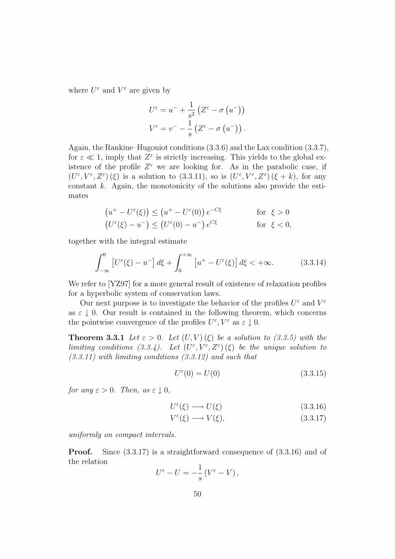
where U ε and V ε are given by

U ε = u− +1

s2

(Zε − σ

(u−))

V ε = v− − 1

s

(Zε − σ

(u−)).

Again, the Rankine–Hugoniot conditions (3.3.6) and the Lax condition (3.3.7),for ε 1, imply that Zε is strictly increasing. This yields to the global ex-istence of the profile Zε we are looking for. As in the parabolic case, if(U ε, V ε, Zε) (ξ) is a solution to (3.3.11), so is (U ε, V ε, Zε) (ξ + k), for anyconstant k. Again, the monotonicity of the solutions also provide the esti-mates (

u+ − U ε(ξ))≤(u+ − U ε(0)

)e−Cξ for ξ > 0(

U ε(ξ)− u−)≤(U ε(0)− u−

)eCξ for ξ < 0,

together with the integral estimate∫ 0

−∞

[U ε(ξ)− u−

]dξ +

∫ +∞

0

[u+ − U ε(ξ)

]dξ < +∞. (3.3.14)

We refer to [YZ97] for a more general result of existence of relaxation profilesfor a hyperbolic system of conservation laws.

Our next purpose is to investigate the behavior of the profiles U ε and V ε

as ε ↓ 0. Our result is contained in the following theorem, which concernsthe pointwise convergence of the profiles U ε, V ε as ε ↓ 0.

Theorem 3.3.1 Let ε > 0. Let (U, V ) (ξ) be a solution to (3.3.5) with thelimiting conditions (3.3.4). Let (U ε, V ε, Zε) (ξ) be the unique solution to(3.3.11) with limiting conditions (3.3.12) and such that

U ε(0) = U(0) (3.3.15)

for any ε > 0. Then, as ε ↓ 0,

U ε(ξ) −→ U(ξ) (3.3.16)

V ε(ξ) −→ V (ξ), (3.3.17)

uniformly on compact intervals.

Proof. Since (3.3.17) is a straightforward consequence of (3.3.16) and ofthe relation

U ε − U = −1

s(V ε − V ) ,

50

it suffices to prove (3.3.16). Writing (3.3.13) in terms of U ε gives

(U ε)′ =1

s(µ− ε2s2)

[s2(u+ − U ε

)−(σ(u+)− σ (U ε)

)]. (3.3.18)

The equation for the viscous profile U is given by

U ′ =1

sµ

[s2(u+ − U

)−(σ(u+)− σ (U)

)]. (3.3.19)

We now integrate both (3.3.18) and (3.3.19) in the interval (0, ξ), for ξ > 0.Then, by employing the condition (3.3.15), we obtain the following integralequation for the difference U ε − U

U ε(ξ)− U(ξ) =

[1

s(µ− ε2s2)− 1

sµ

] ∫ ξ

0

[s2(u+ − U ε(η)

)−(σ(u+)− σ (U ε(η))

)]dη +

1

sµ

∫ ξ

0

[s2 (U ε(η)− U(η))

− (σ (U ε(η))− σ (U(η)))] dη =: I1 + I2.

Now, since the quantity [1

sµ− 1

s(µ− ε2s2)

]is an O (ε2), from the continuity of σ′ and from the estimate

u− < U ε(ξ) < u+,

we obtain

|I1| ≤ O(ε2) ∫ +∞

0

(u+ − U ε(η)

)dη.

Thus, from the integral estimate (3.3.14) we get I1 = O (ε2). Similarly, weobtain

|I2| ≤ O(1)

∫ ξ

0

|U ε(η)− U(η)| dη.

Hence, we apply Gronwall Lemma to obtain the pointwise estimate

|U ε(ξ)− U(ξ)| ≤ C1ε2eC2ξ,

where C1 is a positive constant depending on the limiting conditions, onthe values of U ε and U at ξ = 0 and on the function σ. By means of therelations (3.3.10) we can write the equations (3.3.18) and (3.3.19) in termsof u−. Hence, by integrating on (ξ, 0) for ξ < 0 and by performing the samecalculations of the previous case, we obtain a similar estimate for negative ξand the proof is complete.

51

Remark 3.3.2 The condition

U ε(0) = U(0), (3.3.20)

is to be interpreted as follows. As it is known, in the case of hyperbolic–hyperbolic relaxation (namely in case of ε2µ instead of µ in the third equationof system (3.3.1)), the relaxation profiles are of the form

U ε(x− st) = U

(x− st

ε2

), (3.3.21)

where U solves the same system with ε = 1. Hence, the mass condition∫ 0

−∞

[U ε(ξ + k)− u−

]dξ +

∫ +∞

0

[u+ − U ε(ξ + k)

]dξ = 0,

which select a unique profile among those admissible (here U is the shockprofile of the problem with ε = 0), is automatically satisfied for any ε > 0,

once we require the same condition to be satisfied by U instead of U ε. Inthe present case we cannot express the travelling wave profiles in the form(3.3.21) for a fixed U . Hence, we must require (3.3.20) for any ε > 0.

52

Chapter 4

The Hamer model for radiatinggases

This chapter describes the well–posedness theory and the relaxation limitsfor the radiating gas model presented in the section 1.5 of the introduction.In the following section we describe the global existence theory in L1 ∩ L∞.We also provide an alternative way of determining the well–posedness viathe theory of nonlinear semigroups in the subsection 4.1.1. In section 4.2 weanalyze both the hyperbolic to hyperbolic and the hyperbolic to parabolicrelaxations for this model.

4.1 Global existence of solutions

In this section, we study the existence and uniqueness of weak, entropy so-lutions to the Cauchy problem for the hyperbolic-elliptic coupled system

ut + div f(u) = − div q

−∇ div q + q = −∇u(4.1.1)

where (x, t) ∈ Rd×R+ are the independent variables, u and q are dependentvariables with values in R and Rd respectively and f is a smooth mappingfrom R into Rd, which we assume, without loss of generality, to satisfy f(0) =f ′(0) = 0. We first suppose that the initial datum to the variable u is givenby a function u0 in the space L∞(Rd)∩L1(Rd). The case of L∞ data will becovered later on. We start by rewriting the system (4.1.1) as a scalar balancelaw of the form

ut + div f(u) = −u+K ∗ u, (4.1.2)

53

where the kernel K is given by the Bessel potential

K(x) =1

(4π)d/2

∫ +∞

0

e−s−|x|24s

sd/2ds.

As it is well-known, a bounded measurable function u is a weak solution to(4.1.2) if it verifies the equation in distributional sense and the test functionsare smooth functions with compact support, intersecting the line t = 0. Aweak solution is said to be entropic if, in addition, it verifies the inequality∫ T

0

∫Rd

[η(u)ψt + q(u) · ∇ψ]dxdt+

∫Rd

η(u0(x))ψ(x, 0)dx

≥∫ T

0

∫Rd

η′(u)[u−K ∗ u]ψdxdt, (4.1.3)

for any convex entropy η with flux q : R → Rd given by

qα(u) =

∫ u

f ′α(s)η′(s)ds (4.1.4)

and for any nonnegative Lipschitz continuous test function ψ on Rd × [0, T ]with compact support, intersecting the line t = 0.

In order to show the existence of weak entropy solutions to the equation(4.1.2) with initial datum u0 ∈ L∞(Rd) ∩ L1(Rd), we apply the method ofvanishing viscosity, namely, we study the behavior of the solutions to theparabolic approximation

ut + div f(u) = −u+K ∗ u+ µ∆u (4.1.5)

as µ ↓ 0. We state the following theorem of local existence and uniquenessof solutions to the equation (4.1.5) with initial datum in L1(Rd) ∩ L∞(Rd).The proof of this theorem is contained in the Appendix B.

Theorem 4.1.1 Let the parameter µ > 0 be fixed. Let u0 ∈ L∞(Rd) ∩L1(Rd). Then, there exist a positive time T0 > 0 (depending on µ, u0 and f)such that the equation (4.1.5) has an unique solution u ∈ C([0, T0];L

1(Rd)∩L∞(Rd)) with u0 as initial datum. Moreover, the spatial derivatives of anyorder of u are also in L∞(Rd) ∩ L1(Rd).

We start the analysis of the limit as µ ↓ 0 by proving the followingtheorem.

54

Theorem 4.1.2 Let u and u be solutions to (4.1.5) with initial data u0,u0 ∈ L1(Rd) ∩ L∞(Rd). Then, for any t > 0,∫

Rd

(u(x, t)− u(x, t))+dx ≤∫

Rd

(u0(x)− u0(x))+dx; (4.1.6)

‖u(·, t)− u(·, t)‖L1(Rd) ≤ ‖u0(·)− u0(·)‖L1(Rd). (4.1.7)

Moreover, if u0(x) ≤ u0(x) a.e. on Rd, then u(x, t) ≤ u(x, t) a.e. on Rd ×[0, T ]. In addition, the range of both u and u is contained in [−a, a], where

a = max‖u0‖L∞(Rd), ‖u0‖L∞(Rd).

Proof. Let 0 < T < T0, where T0 is the time of existence of the solutiongiven by the Theorem 4.1.1. We prove the relation (4.1.6) for any t ∈ [0, T ].For ε > 0, we define

ηε(ξ) =

0 if −∞ < ξ ≤ 0ξ2

4εif 0 < ξ ≤ 2ε

ξ − ε if 2ε < ξ < +∞.

We multiply the equation for (u− u) by η′ε(u− u) and obtain

ηε(u− u)t + div[η′ε(u− u)(f(u)− f(u))]− η′′ε (u− u)(f(u)− f(u)) · ∇(u− u)

= µ∆ηε(u− u)− µη′′ε (u− u) |∇(u− u)|2 − η′ε(u− u)[u− u−K ∗ (u− u)].(4.1.8)

Integrating (4.1.8) in x and t, and since η′′ε > 0, we have the following in-equality∫

Rd

ηε(u(x, t)− u(x, t))dx ≤∫

Rd

ηε(u0(x)− u0(x))dx

+

∫ t

0

∫Rd

η′′ε (u− u)(f(u)− f(u)) · ∇(u− u)dxds

−∫ t

0

∫Rd

η′ε[u− u−K ∗ (u− u)]dxds. (4.1.9)

Now, as ε ↓ 0, we have, pointwise,

ηε(u(x, t)− u(x, t)) → (u(x, t)− u(x, t))+

η′ε(u(x, t)− u(x, t)) → sgn(u(x, t)− u(x, t))+

η′′ε (u(x, t)− u(x, t))(f(u)− f(u)) → 0.

55

Now, since f is a smooth mapping (in particular, f is Lipschitz continuous),the quantity

η′′ε (u(x, t)− u(x, t))|f(u)− f(u)|is bounded uniformly in ε. Therefore, letting ε ↓ 0 in (4.1.9), we obtain∫

Rd

(u− u)+dx ≤∫

Rd

(u0 − u0)+dx

−∫ t

0

∫Rd

[(u− u)+ − sgn(u− u)+K ∗ (u− u)]dxds. (4.1.10)

We now estimate the convolution term in the above relation as follows∫ t

0

∫Rd

sgn(u− u)+K ∗ (u− u)dxdτ

=

∫ t

0

∫Rd

sgn(u− u)+

∫Rd

K(x− y)(u− u)(y, τ)dydxdτ

≤∫ t

0

∫Rd

∫Rd

K(x− y)(u− u)+(y, τ)dydxdτ

=

∫ t

0

∫Rd

(u− u)+(y, s)dydτ,

where we have used the property of the convolution kernel∫Rd

K(z)dz = 1.

Thus, the integral inequality (4.1.10) reduces to∫Rd

(u− u)+dx ≤∫

Rd

(u0 − u0)+dx

which is exactly (4.1.6). Interchanging the roles of u and u we derive a similarinequality which added to (4.1.6) yields (4.1.7). The monotonicity propertystated in the theorem is again a consequence of (4.1.6). To prove the lastassertion of the theorem, namely the bound of the solutions in L∞(Rd), weperform an uniform control of the Lp norms of the solutions. For ε > 0, letθε(ξ) be a convex regularization of the function |ξ|p, 1 < p <∞. We multiplythe equation (4.1.5) by θ′ε(u) to obtain

θε(u)t + div (F (u)) = −θ′ε(u) (u−K ∗ u) + µ∆ (θε(u))− µθ′′ε (u) |∇u|2 ,

where

Fj(ξ) =

∫ ξ

θ′ε(s)f′j(s)ds,

56

for j = 1, ..., d. Integrating in x and t and letting ε ↓ 0 we obtain∫Rd

|u|pdx ≤∫

Rd

|u0|pdx

−∫ t

0

∫Rd

p|u|pdxds+

∫ t

0

∫Rd

p|u|p−1|K ∗ u|dxds. (4.1.11)

We estimate the convolution integral as follows∫Rd

|u|p−1|K ∗ u|dx ≤ ‖u‖p−1Lp ‖K ∗ u‖Lp ≤ ‖u‖p−1

Lp ‖u‖Lp‖K‖L1 = ‖u‖pLp ,

where again we used the identity∫

Rd K(x)dx = 1. Hence, (4.1.11) becomes

‖u‖Lp ≤ ‖u0‖Lp ≤ ‖u0‖p−1

p

L∞ ‖u0‖1p

L1 .

Thus we estimate the L∞ norm of u as follows

‖u‖L∞ ≤ lim supp→+∞

‖u‖Lp ≤ limp→+∞

‖u0‖p−1

p

L∞ ‖u0‖1p

L1 = ‖u0‖L∞

and the last assertion of the theorem follows. Finally, both this last L∞

estimate and the L1 estimate coming from (4.1.7) imply in particular thatthe local-in-time solution provided by the Theorem 4.1.1 is indeed global andall the estimate we have proved are satisfied for any t > 0.

In the following lemma we provide the estimate (uniformly with respectto µ) of the L1-modulus of continuity of the solution uµ to (4.1.5) withu0 ∈ L∞(Rd) ∩ L1(Rd).

Lemma 4.1.3 Let uµ be the solution to (4.1.5) with u0 ∈ L1(Rd) ∩ L∞(Rd)as initial datum. In particular∫

Rd

|u0(x+ h)− u0(x)|dx ≤ ω(|h|), for any h ∈ Rd, (4.1.12)

for some nondecreasing function ω on [0,+∞) with ω(r) ↓ 0 as r ↓ 0. Thenthere exists a constant C, depending on ‖u0‖L∞(Rd) and on the mapping fsuch that, for any t > 0,∫

Rd

|uµ(x+ h, t)− uµ(x, t)|dx ≤ ω(|h|), for any h ∈ Rd (4.1.13)

and∫Rd

|uµ(x, t+k)−uµ(x, t)|dx ≤ C(k+k23 +µk

13 )‖u0‖L1(Rd)+4ω(k

13 ), (4.1.14)

for any k > 0.

57

Proof. Fix t > 0. Applying (4.1.7) with u(x, t) = u(x + h, t), we obtain(4.1.13).

Now, let k > 0 be fixed and let φ be a smooth, bounded function onRd. Then, multiplying the equation (4.1.5) by φ and integrating by parts theresulting equation on the domain Rd × (t, t+ k), we get∫

Rd

φ(x)[u(x, t+ k)− u(x)]dx

=

∫ t+k

t

∫Rd

[∇φ(x) · f(u(x, τ)) + µ∆φ(x)u(x, τ)

+ φ(x)(−u(x, τ) + (K ∗ u)(x, τ))]dxdτ. (4.1.15)

We now set φ to be a suitable regularization of the function sgn[u(x, t +k)−u(x, t)], in order to get the desired estimate (4.1.14). More precisely, wechoose

φ(x) =

∫Rd

k−d3

d∏j=1

ρ

(xj − ξj

k13

)sgn(u(ξ, t+ k)− u(ξ, t))dξ,

where ρ is a smooth, nonnegative function on R with support contained in[−1, 1] and total mass one. Since |φ| ≤ 1, |∇φ| ≤ c1k

− 13 and |∆φ| ≤ c2k

− 23 ,

from (4.1.15) we obtain∫Rd

φ(x)(u(x, t+ k)− u(x, t))dx ≤ C(k + k23 + µk

13 )‖u0‖L1(Rd), (4.1.16)

where the constant C depends on ‖u0‖L∞ and on the Lipschitz constant ofthe mapping f . Then, we observe that

|u(x, t+ k)− u(x, t)| − φ(x)(u(x, t+ k)− u(x, t))

=

∫Rd

k−d3

d∏j=1

ρ

(xj − ξj

k13

)[|u(x, t+ k)− u(x, t)|

− (u(x, t+ k)− u(x, t)) sgn(u(ξ, t+ k)− u(ξ, t))]dξ

≤ 2

∫Rd

k−d3

d∏j=1

ρ

(xj − ξj

k13

)|u(x, t+ k)− u(x, t)− (u(ξ, t+ k)− u(ξ, t))|dξ.

Therefore, after integration on Rd and from (4.1.13), we obtain the inequality∫Rd

[|u(x, t+ k)− u(x, t)| − φ(x)(u(x, t+ k)− u(x, t)] dx ≤ 4ω(k13 )

58

which, combined with (4.1.16), implies (4.1.14).

By virtue of Lemma 4.1.3, the family uµ is compact in L1loc(Rd×[0,∞)),

and then, passing if necessary to a subsequence, it converges strongly (andboundedly almost everywhere in Rd× [0,∞), from Theorem 4.1.2) to a func-tion u ∈ L1(Rd × [0, T ]) ∩ L∞(Rd × [0, T ]). Moreover, due to the strongconvergence of the sequence and due to its boundedness in L∞, it is easy toverify that the limit function u is an entropy solution to (4.1.2) with u0 asinitial datum. Hence, the following theorem holds.

Theorem 4.1.4 Let uµ be the solution to (4.1.5) with u0 ∈ L1(Rd)∩L∞(Rd)as initial datum. Then, as µ ↓ 0 (passing if necessary to a subsequence), forany T > 0,

uµ −→ u, strongly in Lploc(Rd × [0, T ]), p < +∞,

and u ∈ L1(Rd × [0, T ]) ∩ L∞(Rd × [0, T ]) is an entropy solution to (4.1.2)with u0 as initial datum.

We now pass to the study of the uniqueness of the weak, entropy solutionsto (4.1.2) with initial datum u0 ∈ L1(Rd)∩L∞(Rd). As in the homogeneouscase (see [Kru70], [Daf00]), we have the following theorem.

Theorem 4.1.5 Let u, u ∈ L∞([0, T ];L1(Rd) ∩ L∞(Rd)) be weak entropysolutions to (4.1.2) with initial data u0, u0 ∈ L1(Rd) ∩ L∞(Rd). Then, forany t ∈ [0, T ],∫

Rd

(u(x, t)− u(x, t))+dx ≤∫

Rd

(u0(x)− u0(x))+dx; (4.1.17)

‖u(·, t)− u(·, t)‖L1(Rd) ≤ ‖u0(·)− u0(·)‖L1(Rd). (4.1.18)

Moreover, if u0(x) ≤ u0(x) a.e. on Rd, then u(x, t) ≤ u(x, t) a.e. on Rd ×[0, T ]. In addition, the essential range of both u and u is contained in [−a, a],where

a = max‖u0‖L∞(Rd), ‖u0‖L∞(Rd).

Proof. We proceed by using the following relation, as in the homogeneouscase, ∫ T

0

∫Rd

[ψt(u− u)+ + sgn(u− u)+∇ψ · (f(u)− f(u))]dxdt

+

∫Rd

ψ(x, 0)(u0 − u0)+dx

≥∫ T

0

∫Rd

ψ[(u− u)+ − sgn(u− u)+K ∗ (u− u)]dxdt, (4.1.19)

59

for any nonnegative Lipschitz continuous test function ψ on Rd× [0, T ] withcompact support, intersecting the line t = 0. The inequality (4.1.19) isobtained by considering the entropy (u(x, t)−u(y, s))+ either in the (x, t) andin the (y, s) variables, and by choosing a suitable test function, convergingto δ functions centered at y = x and at t = s (see [Kru70] and [Daf00]).Now, we employ (4.1.19) as follows. Let R > 0, t ∈ [0, T ) and ε > 0 be fixed,and let us write (4.1.19) with the test function given by ψ(x, τ) = χ(x, τ)θ(τ),where

χ(x, τ) =

1 if 0 ≤ τ < T, 0 ≤ |x| < R + s(t− τ)1ε[R + s(t− τ)− |x|] + 1 if 0 ≤ τ < T,

R + s(t− τ) ≤ |x| < R + s(t− τ) + ε

0 if 0 ≤ τ < T, |x| ≥ R + s(t− τ) + ε,

θ(τ) =

1 if 0 ≤ τ < t1ε(t− τ) + 1 if t ≤ τ < t+ ε,

0 if t+ ε ≤ τ < T,

and

s = max

|f(u)− f(u)||u− u|

, (4.1.20)

for u and u in the range of solutions. Computing explicitly the derivativesof ψ (see [Daf00]), we get

1

ε

∫ t+ε

t

∫|x|<R+s(t−τ)

(u− u)+dxdτ ≤∫|x|<R+st

(u0 − u0)+dx

−1

ε

∫ T

0

∫R+s(t−τ)≤|x|<R+s(t−τ)+ε

[s(u− u)++ sgn(u− u)+ x

|x|· (f(u)−f(u))

]dxdτ

−∫ T

0

∫Rd

χ(x, τ)θ(τ)[(u− u)+ − sgn(u− u)+K ∗ (u− u)]dxdτ +O(ε)

≤∫|x|<R+st

(u0 − u0)+dx− I(u− u) +O(ε). (4.1.21)

The last inequality is due to the special choice of the constant s, which implies[s(u− u)+ +

x

|x|· (f(u)− f(u)) sgn(u− u)+

]> 0.

Moreover, we denoted the contribution due to the source term by I(u − u).The special form of the function ψ yields to

I(u− u) =

∫ t

0

∫|x|<R+s(t−τ)

[(u− u)+ − sgn(u− u)+K ∗ (u− u)]dxdτ +O(ε).

60

Hence, letting ε ↓ 0, we have∫|x|<R

(u− u)+dx ≤∫|x|<R+st

(u0 − u0)+dx−

∫ t

0

∫|x|<R+s(t−τ)

(u− u)+dxdτ

+

∫ t

0

∫|x|<R+s(t−τ)

sgn(u− u)+K ∗ (u− u)]dxdτ. (4.1.22)

From the above inequality, with R→∞, we obtain∫Rd

(u− u)+dx ≤∫

Rd

(u0 − u0)+dx−

∫ t

0

∫Rd

(u− u)+dxdτ

+

∫ t

0

∫Rd

sgn(u− u)+K ∗ (u− u)]dxdτ. (4.1.23)

We estimate the convolution term as follows∫ t

0

∫Rd

sgn(u− u)+K ∗ (u− u)]dxdτ

=

∫ t

0

∫Rd

sgn(u− u)+

∫Rd

K(x− y)(u− u)(y, τ)dydxdτ

≤∫ t

0

∫Rd

∫Rd

K(x− y)(u− u)+(y, τ)dydxdτ

=

∫ t

0

∫Rd

(u− u)+(y, τ)dydτ.

Hence, (4.1.17) is proved. As usual, interchanging the roles of u and u weobtain the L1-contraction property (4.1.18), while the monotonicity propertystated in the theorem is again a direct consequence of (4.1.17). Now, as inthe case of the viscous approximation, we perform the L∞ estimate by meansof a uniform bound for the Lp norms. As in the Theorem 4.1.2, we obtain∫

Rd

|u|pdx ≤∫

Rd

|u0|pdx−∫ t

0

∫Rd

p|u|pdxds+

∫ t

0

∫Rd

p|u|p−1|K ∗ u|dxds,

which yields to the desired L∞ estimate, and the proof is complete.

As a consequence of the last theorem, we have the following

Corollary 4.1.6 There exists at most one entropy solution of (4.1.2), be-longing in the space L∞([0, T ];L1(Rd) ∩ L∞(Rd)), having initial datum inL1(Rd) ∩ L∞(Rd).

61

Remark 4.1.7 As a consequence of the uniqueness result we have estab-lished, we can conclude that any weak, entropy solution to (4.1.2) belongingin the space L∞([0, T ];L1(Rd) ∩ L∞(Rd)) verifies the estimate∫

Rd

|u(x, t+ k)− u(x, t)|dx ≤ C(k + k23 )‖u0‖L1(Rd) + 4ω(k

13 )

(where ω represents the L1–modulus of continuity of the initial datum),which can be easily obtained by sending µ → 0 in (4.1.14). Thus, u ∈C([0, T ];L1(Rd)) for any T > 0.

4.1.1 Well–posedness via nonlinear semigroups

In view of the previous results, the solutions to (4.1.2) may be viewed as thetrajectories of a contraction semigroup S(t), t > 0 defined on the spaceL∞(Rd) ∩ L1(Rd) endowed with the L1–norm. Our next aim is to show thatthe existence and uniqueness of weak, entropy solutions to the balance law(4.1.2), together with its contraction properties, can be obtained through thetheory of nonlinear contraction semigroups in Banach spaces ([Cra72, CL71]).

To construct the semigroup, we should realize (4.1.2) as an abstract dif-ferential equation

du

dt+ A(u) 3 0, (4.1.24)

for a suitably defined transformation A, with domain D(A) and range R(A)both contained in L1(Rd). This operator may, in general, be multivalued,even though, for u smooth one should expect A(u) = div f(u) + u −K ∗ u.However, while performing the extension of A to those function that arenot smooth, we must consider the admissibility condition encoded in therelation (4.1.3). This leads us to the following abstract definition of the

transformation A. We first define the simpler extension A.

Definition 4.1.8 The (possibly multivalued) transformation (A,D(A)), with

domain D(A) contained in L1(Rd), is determined by u ∈ D(A) and w ∈ R(A)if u, w and f(u) are all in L1(Rd) and if the inequality∫

Rd

∇ψ(x) · q(u(x)) + η′(u(x)) [−u(x) + (K ∗ u)(x)]ψ(x)

+ ψ(x)η′(u(x))w(x) dx ≥ 0, (4.1.25)

holds for any convex entropy function η, such that η′ is bounded on R, withassociated entropy flux q : R → Rd determined as in (4.1.4) and for all non-negative Lipschitz continuous test functions ψ on Rd with compact support.

62

Applying (4.1.25) for the pairs (±u,±f(u)), we recover that

A(u) = div f(u) + u−K ∗ u

in the sense of distributions for any u ∈ D(A). In particular, A is a single–valued transformation. Moreover, the relation (4.1.4) implies, for any u ∈C1

0(Rd) and for any nonnegative test function ψ,∫Rd

∇ψ · q(u) + ψη′(u) div f(u) dx = 0,

which yields∫Rd

∇ψ · q(u) + ψη′(u)[A(u)− u+K ∗ u]

dx = 0.

Hence, C10(Rd) ∈ D(A) and, in particular, D(A) is dense in L1(Rd). Thus,

we finally define the transformation A as follows

Definition 4.1.9 The (possibly multivalued) transformation (A,D(A)), with

domain D(A) contained in L1(Rd), is the graph closure of A, i.e., u ∈ D(A)and w ∈ A(u) iff (u,w) is the limit in L1(Rd) × L1(Rd) of a sequence

(uk, wk) such that uk ∈ D(A) and wk ∈ A(uk).

We now establish the properties of A which guarantee that it is the gen-erator of a contraction semigroup.

Theorem 4.1.10 The transformation A is accretive, that is, if u and u arein D(A), then, for any λ > 0, w ∈ A(u), w ∈ A(u), the following inequalityholds

‖(u+ λw)− (u+ λw)‖L1(Rd) ≥ ‖u− u‖L1(Rd). (4.1.26)

Proof. It is sufficient to prove (4.1.26) for u, u ∈ D(A). Thus, let w = A(u),w = A(w). We proceed by considering the following relation, as in thehomogeneous case (see [Daf00]),∫

Rd

∫Rd

sgn(u(x)− u(x)) (∇x +∇x)φ(x, x) · (f(u(x))− f(u(x)))

−2 [u(x)− u(x)− (K ∗ u)(x) + (K ∗ u)(x)]φ(x, x)

+φ(x, x)[w(x)− w(x)] dxdx ≥ 0, (4.1.27)

63

which holds for any test function φ ≥ 0 on Rd ×Rd. The inequality (4.1.27)is obtained by writing the relation (4.1.25) for the entropy–entropy flux pairs

η(u; u(x)) = |u− u(x)|,q(u; u(x)) = sgn(u− u(x))(f(u)− f(u(x)))

and by interchanging the roles of u and u. We now choose the test functionφ as follows, for fixed ε > 0,

φ(x, x) = ε−dψ

(x+ x

2

) d∏α=1

ρ

(xα − xα

2ε

),

where ρ is a standard mollifier as in the proof of Lemma 4.1.3 and ψ is asmooth function on Rd such that ψ(x) = 1 for |x| < R, and ψ(x) = 0 for|x| > R + 1. Since∫

Rd

∫Rd

[u(x)− u(x)− (K ∗ u)(x) + (K ∗ u)(x)] dxdx ≥ 0,

by explicitly computing the derivatives of φ, by letting ε ↓ 0 and then bysending R→∞, we obtain∫

Rd

sgn(u(x)− u(x))[w(x)− w(x)]dx ≥ 0.

Now, let λ > 0. From the last inequality we recover

‖(u+ λw)− (u+ λw)‖L1(Rd)

≥∫

Rd

sgn(u(x)− u(x))u(x)− u(x) + λ[w(x)− w(x)]dx

≥∫Rd

sgn(u(x)− u(x))[u(x)− u(x)]dx = ‖u− u‖L1(Rd).

The proof is complete.

Theorem 4.1.11 The transformation A is maximal, that is

R(I + λA) = L1(Rd), for any λ > 0.

Proof. It will suffice to show that R(I + λA) is dense in L1(Rd); indeed, wewill prove L1(Rd) ∩ L∞(Rd) ⊂ R(I + λA). Let g ∈ L1(Rd) ∩ L∞(Rd). We

seek solutions u ∈ D(A) of the equation

u+ λA(u) = g (4.1.28)

64

We construct solutions to this equation as the µ ↓ 0 limit of the ellipticequations

u(x) + λ div f(u(x)) + u(x)− (K ∗ u)(x) − µ∆u(x) = g(x), x ∈ Rd.(4.1.29)

From the standard theory of elliptic equations, (4.1.29) admits a solution inH2(Rd). The convergence of uµ to some function u which is the solution to(4.1.28) comes from the following two lemmas.

Lemma 4.1.12 Let u, u be solutions to (4.1.29) with respective source termsg and g that are in L1(Rd) with range contained in the interval [a, b]. Then∫

Rd

[u(x)− u(x)]+dx ≤∫

Rd

[g(x)− g(x)]+dx,

‖u− u‖L1(Rd) ≤ ‖g − g‖L1(Rd). (4.1.30)

Moreover, ifg(x) ≤ g(x), on Rd

thenu(x) ≤ u(x), on Rd.

Moreover, the range of both u and u is contained in [a, b].

We skip the detail of the proof of this lemma, which are very similar tothose in the proof of Theorem 4.1.2. Once again, the contraction propertiesof the source term −u+K ∗u are employed. Hence, in a similar way as in thecase of the vanishing viscosity approximation, we obtain the compactness ofthe sequence uµ needed to pass the limit as µ ↓ 0 in the equation (4.1.29).

Lemma 4.1.13 Let uµ denote the solution of (4.1.29), with source termgiven by g ∈ L∞(Rd) ∩ L1(Rd). Then, as µ ↓ 0, uµ converges boundedlya.e. to the solution u of (4.1.28).

Proof. By applying (4.1.30) with g(x) = g(x+ y), we obtain∫Rd

|uµ(x+ y)− uµ(x)|dx ≤∫

Rd

|g(x+ y)− g(x)|dx.

Thus the family uµ is compact in L1loc. Hence, passing if necessary to

subsequences, uµ → u boundedly a.e. on Rd. To complete the proof, wehave to show that u is the unique solution to (4.1.28). Consider any smooth

65

convex entropy η(u) with associated entropy flux q determined by (4.1.4).Then uµ satisfies the identity

η′(uµ)uµ + λ div q(uµ) + λη′(uµ)(u− (K ∗ u))− µ∆η(uµ)

+ µη′′(uµ) |∇uµ|2 = η′(uµ)g.

Hence, multiplying the last identity by any nonnegative smooth test functionψ on Rd, with compact support, and integrating over Rd yields∫

Rd

λ∇ψ · q(uµ) + ψη′(uµ)(g − uµ − λ(uµ − (K ∗ uµ))) dx

≥ −µ∫

Rd

∆ψηdx.

Finally, by sending µ ↓ 0 we get∫Rd

∇ψ · q(u) + ψη′(u)

[1

λ(g − u)− (u− (K ∗ u))

]≥ 0,

which means that u is a solution to (4.1.28). Now, as a consequence of theprevious theorem, the solution u to (4.1.28) is unique. Therefore, the entiresequence uµ converges to u as µ ↓ 0. This completes the proof of the lemmaand the proof of Theorem 4.1.11.

Finally, once we have established accretiveness and maximality for thetransformation A, we can employ the Crandall–Liggett theory of semigroupsin nonreflexive Banach spaces to obtain that A generates a contraction semi-group S(·) on D(A) = L1(Rd). We summarize the properties of the S(·) inthe following theorem, whose proof can be found in [Cra72, CL71].

Theorem 4.1.14 The transformation A generates a contraction semigroup

S(·) : L1(Rd) → L1(Rd), t ∈ [0,+∞)

which is continuous with respect to t. Moreover, for any u0, u0 ∈ L1(Rd) suchthat

u0 ≤ u0 a.e. on Rd,

we haveS(t)u0 ≤ S(t)u0, a.e. on Rd.

Moreover, for 1 ≤ p ≤ ∞, the sets Lp(Rd) ∩ L1(Rd) are positively invariantunder S(t) and, for any t ≥ 0,

‖S(t)u0‖Lp(Rd) ≤ ‖u0‖Lp(Rd), for all u0 ∈ Lp(Rd) ∩ L1(Rd).

If u0 ∈ L∞(Rd)∩L1(Rd), then S(·)u0 is the admissible weak, entropy solutionof (4.1.2) with initial datum u0.

66

4.1.2 Extension to L∞

We now conclude this section by discussing the general case of initial data inL∞(Rd). More precisely, we extend the semigroup S(t) to the space L∞(Rd)endowed with the following norm

‖|u‖| =∫

Rd

φ(x)|u(x)|dx, (4.1.31)

where φ is a positive, smooth function on Rd satisfying

φ(x) = e−|x| for any |x| ≥ 2,

φ(x) = 1 for any |x| ≤ 1.

We remark that the uniqueness of solutions with initial data in L∞ has beenproved only in the one–dimensional case (see [Ser03]). This problem is stillopen in the multi–dimensional case. The extension of the semigroup to L∞

leaves entirely open the question of uniqueness in L∞. We show the continuityof the semigroup St on the space (L∞ ∩ L1, ‖| · ‖|), which is a dense subspaceof(L∞(Rd), ‖| · ‖|

). We also observe that the following procedure extends

the semigroup St to the Banach space L1(Rd, φdx) which is the closure of ourspace

(L∞(Rd), ‖| · ‖|

)with respect to the norm ‖| · ‖|.

Theorem 4.1.15 Let u, u ∈ L∞([0, T ];L1(Rd) ∩ L∞(Rd)) be weak entropysolutions of (4.1.2) with initial data u0, u0 ∈ L1(Rd) ∩ L∞(Rd). Then, forany t ∈ [0, T ],

‖|u(·, t)− u(·, t)‖| ≤ eCt‖|u0 − u0‖|, (4.1.32)

where the constant C depends on φ, on the mapping f and on ‖u0‖L∞,‖u0‖L∞.

Proof. Due to the uniqueness result, we can view the solutions u, u as thelimit of their viscous approximations uµ, uµ respectively. We then multiplythe equation for uµ − uµ by the weight function φ to obtain

[φ(uµ − uµ)]t + div [φ(f(uµ)− f(uµ))]

= −φ [uµ − uµ −K ∗ (uµ − uµ)]

+∇φ · (f(uµ)− f(uµ))+µφ∆(uµ − uµ). (4.1.33)

Let ηε(ξ) be a convex regularization of the function |ξ| (in the spirit of thefunction used in the proof of Theorem 4.1.2. Multiplying (4.1.33) by η′ε(u

µ−

67

uµ) we obtain

φηε,t + div [φη′ε(f(uµ)− f(uµ))]

= −φη′ε [uµ − uµ −K ∗ (uµ − uµ)]

+ φη′′ε (f(uµ)− f(uµ)) · ∇(uµ − uµ)

+ η′ε∇φ · (f(uµ)− f(uµ))

+ µ div [φη′ε∇(uµ − uµ)]−µη′ε∇φ · ∇(uµ − uµ)

− µη′′εφ |∇(uµ − uµ)|2 . (4.1.34)

Thus, proceeding as in the proof of Theorem 4.1.2 we integrate (4.1.34) indx and dt and we let ε ↓ 0 to obtain (after integration by parts)∫

Rd

φ(x)|uµ − uµ|dx ≤∫

Rd

φ(x)|u0 − u0|dx

+ C

∫ t

0

∫Rd

(|∇φ|+ |∆φ|) |uµ − uµ|dsdx, (4.1.35)

where the constant C depends on ‖u‖∞, ‖u0‖∞ and on the mapping f , forµ < 1. Since (|∇φ| + |∆φ|) ≤ C1φ, from (4.1.35) and from the Gronwalllemma, we obtain (4.1.32) as µ ↓ 0.

4.2 Relaxation Limits

In this section we analyze the convergence of the relaxation limits for ourmodel

Us + div f(U) = − divQ

−∇ divQ+Q = −∇U,(4.2.1)

where (y, s) ∈ Rd × R+ are the independent variables.

4.2.1 Hyperbolic-hyperbolic relaxation limit

We start the analysis with the hyperbolic-hyperbolic relaxation. Therefore,in order to obtain an hyperbolic-type limit, we perform the following scaling

uε(x, t) = U

(x

ε,t

ε

)qε(x, t) = Q

(x

ε,t

ε

).

68

Thus, the system (4.2.1) becomesuεt + div f(uε) = − div qε

−ε2∇ div qε + qε = −ε∇uε.(4.2.2)

We give an initial datum u0(x) ∈ L1(Rd) ∩ L∞(Rd). We postpone the dis-cussion of L∞ initial data at the end of the subsection.

Remark 4.2.1 In the construction of the Cauchy problem for (4.2.2), wescale only the terms for t > 0, without scaling the initial datum, which isgiven a posteriori as a fixed function in L1(Rd)∩L∞(Rd). Indeed, the scaledinitial datum is given by the sequence uε0(x) = U0

(xε

), which converges to zero

strongly in L1(Rd) because U0 ∈ L1(Rd). Thus, in this way we can recoverat the limit only the null solution. In other words, we do not investigate therelaxation limit of the scaled solution, but we use the scaling only to detectthe terms which are physically negligible in the equations and we study thesingular limit of the new Cauchy problem, with fixed datum.

Letting ε ↓ 0 in the system (4.2.2), we see that formally we obtain q = 0 andthe limit equation is given by

ut + div f(u) = 0. (4.2.3)

To justify rigorously this limit, it is convenient once again to write the system(4.2.2) as the balance law

uεt + div f(uε) = −1

ε(uε −Kε ∗ uε) , (4.2.4)

where the convolution kernel is given by

Kε(x) =1

εdK(xε

),

and K is again

K(x) =1

(4π)d/2

∫ +∞

0

e−s−|x|24s

sd/2ds.

We observe that the new convolution kernel Kε is scaled such that ‖Kε‖L1 =‖K‖L1 = 1. Thus, the contraction properties of the source term we employedin the previous section are still valid. Therefore, the same properties estab-lished in the Theorem 4.1.2 for the viscous approximation are satisfied bythe family uε, as we state in the following result. We skip the details ofthe proof, which follows the same ideas of Theorem 4.1.2.

69

Theorem 4.2.2 Let ε > 0. Let uε, uε ∈ L∞([0, T ];L1(Rd) ∩ L∞(Rd)) beweak entropy solutions of (4.2.4) with initial data u0, u0 ∈ L1(Rd)∩L∞(Rd).Then, for any t ∈ [0, T ],∫

Rd

(uε(x, t)− uε(x, t))+dx ≤∫

Rd

(u0(x)− u0(x))+dx;

‖uε(·, t)− uε(·, t)‖L1(Rd) ≤ ‖u0(·)− u0(·)‖L1(Rd).

Moreover, if u0(x) ≤ u0(x) a.e. on Rd, then uε(x, t) ≤ uε(x, t) a.e. on Rd ×[0, T ]. In addition, the essential range of both uε and uε is contained in[−a, a], where

a = max‖u0‖L∞(Rd), ‖u0‖L∞(Rd).

Again, as in the study of the vanishing viscosity approximation, we carry outthe following estimates for the L1– modulus of continuity of the solutions.

Lemma 4.2.3 Let uε ∈ L∞([0, T ];L1(Rd) ∩ L∞(Rd)) be the weak, entropysolution to (4.2.4) with u0 ∈ L1(Rd)∩L∞(Rd) as initial datum. In particular∫

Rd

|u0(x+ h)− u0(x)|dx ≤ ω(|h|), for any h ∈ Rd,

for some nondecreasing function ω on [0,+∞) with ω(r) ↓ 0 as r ↓ 0. Thenthere exists a constant C, depending only on ‖u0‖L∞(Rd) and on the mappingf such that, for any t > 0,∫

Rd

|uε(x+ h, t)− uε(x, t)|dx ≤ ω(|h|), for any h ∈ Rd (4.2.5)

and ∫Rd

|uε(x, t+ k)− uε(x, t)|dx ≤ Ck23‖u0‖L1(Rd) + 4ω(k

13 ), (4.2.6)

for any k > 0.

Proof. As in the proof of Lemma 4.1.3, the results of Theorem 4.2.2 implies(4.2.5). Now, due to the time regularity of the weak, entropy solution uε (seethe Remark 4.1.7), we have∫

Rd

φ(x)[uε(x, t+ k)− uε(x)]dx =

∫ t+k

t

∫Rd

[∇φ(x) · f(uε(x, τ))

+φ(x)

ε(−uε(x, τ) + (Kε ∗ uε)(x, τ))

]dxdτ, (4.2.7)

70

where φ is the same regularization of the sign function considered in the proofof Lemma 4.1.3. The only difference with the case of the vanishing viscosityapproximation stands in the source terms, which, however, can be controlledin a similar way, due to its good contraction properties. Indeed, we have

− 1

ε

∫ t+k

t

∫Rd

φ(x) (uε −Kε ∗ uε) dxdτ

= −1

ε

∫ t+k

t

∫Rd

φ(x)

∫Rd

K(ξ) (uε(x, τ)− uε(x− εξ, τ)) dξdxdτ

= −1

ε

∫ t+k

t

∫Rd

∫Rd

(φ(x+ εξ)− φ(x))K(ξ)uε(x, τ)dxdτdξ

= ε1

ε

∫ t+k

t

∫Rd

∫Rd

K(ξ)uε(x, τ)∇φ(ζ) · ξdxdtdξ

≤ Ck23‖u0‖L1(Rd),

where the constant C is independent from ε. Finally, the relation (4.2.6) canbe proved as before starting from (4.2.7) and the proof is complete.

Now we can prove our first relaxation result.

Theorem 4.2.4 Let uε ∈ L∞([0, T ];L1(Rd) ∩ L∞(Rd)) be the weak, entropysolution of (4.2.4) with initial datum u0 ∈ L1(Rd)∩L∞(Rd). Then, as ε ↓ 0,

uε −→ u, strongly in Lploc(Rd × [0, T ]), p < +∞.

Moreover, u ∈ L∞([0, T ];L1(Rd)∩L∞(Rd)) is the unique entropy solution to(4.2.3) with u0 as initial datum.

Proof. Applying the results of Lemma 4.2.3 and of the Theorem 4.2.2, weobtain the compactness of the sequence uε in L1

loc and its boundedness inL∞. Thus, passing to subsequence, we have

uε −→ u, strongly in Lploc(Rd × [0, T ]), p < +∞,

and boundedly almost everywhere on Rd × [0,∞). Now, as usual in thisframework, this conditions guarantee that the first-order terms in the weak,entropy formulation of (4.2.4) converge, as ε ↓ 0, to the distribution ut +div f(u). Hence, we can conclude that the limit function u is the uniqueentropy solution of (4.2.3) if, as ε ↓ 0,

−1

ε(uε −Kε ∗ uε) −→ 0 (4.2.8)

71

in the sense of distributions. We remark that once we prove that u is theunique entropy solution to (4.2.3), the whole sequence uε will converge tou. To analyze the convergence of the source term, let ψ(x, t) be a smooth,compactly supported test function. Then, we have

− 1

ε

∫ T

0

∫Rd

ψ(x, t) (uε −Kε ∗ uε) dxdτ

= −1

ε

∫ T

0

∫Rd

ψ(x, t)

∫Rd

K(ξ) (uε(x, τ)− uε(x− εξ, τ)) dξdxdτ

= −1

ε

∫ T

0

∫Rd

∫Rd

(ψ(x+ εξ)− ψ(x, t))K(ξ)uε(x, τ)dxdτdξ.

Now, we observe that

|ψ(x+ εξ, t)− ψ(x, t)− ε∇ψ(x, t) · ξ| ≤ 1

2ε2 |ξ|2 ‖ψ‖C2

0

and hence we have∣∣∣∣1ε∫ T

0

∫Rd

ψ(x, t) (uε −Kε ∗ uε) dxdτ∣∣∣∣

≤∣∣∣∣ε1ε

∫ T

0

∫Rd

∫Rd

K(ξ)uε(x, t)ξ · ∇ψ(x, t)dxdψdt

∣∣∣∣+ε

2‖ψ‖C2

∫ T

0

∫Rd

|uε(x, t)|dxdt∫

Rd

|ξ|2K(ξ)dξ := I1 + I2.

Now, since ∫Rd

K(ξ)ξjdξ = 0, j = 1, ..., d,

then, I1 = 0. Moreover, since the function K(ξ)|ξ|2 has finite mass, the termI2 is bounded by O(ε)T‖ψ‖C2‖u0‖L1(Rd). This proves (4.2.8).

Remark 4.2.5 In the proof of the hyperbolic–hyperbolic relaxation limit,we take advantage of the L1 contraction of the source of (4.2.4), which aredue solely to the property of the convolution kernel Kε, namely

• Kε(x) = Kε(|x|);

• Kε ≥ 0;

• ‖Kε‖L1 = 1.

72

Moreover, the above conditions imply also that the first momenta of Kε arezero and this feature allows to control the singular limit of the source in thesense of distribution (see the last line in the proof of Theorem 4.2.4). Thus,the results we obtained are still valid for any equation of the form (4.2.4),with a convolution kernel satisfying the above conditions.

We conclude this subsection with the case of L∞ initial data. Althoughwe cannot state a relaxation result for any solution in L∞ (because of thelack in the well–posedness in the multi–dimensional case), we can restrictourselves to the case of L∞ solutions defined via the extended semigroupdetermined by the result in Theorem 4.1.15. In other words, given u0 ∈ L∞,we consider the L∞ solution with initial datum u0 defined via the densityargument performed at the end of the previous section. As we pointed outbefore, the only difference with the non-scaled equation lies in the sourceterm, due to the singular coefficient 1

εand the scaled kernel Kε. However,

these changements do not affect the monotonicity properties of the sourceterm and therefore we can repeat the argument of the previous section toprove the following theorem.

Theorem 4.2.6 Let uε, uε ∈ L∞([0, T ] × Rd) be weak entropy solutions of(4.2.4) with initial data u0, u0 ∈ L∞(Rd), uε, uε determined by the extendedsemigroup defined by Theorem 4.1.15. Then, for any t ∈ [0, T ],

‖|uε(·, t)− uε(·, t)‖| ≤ eCt‖|u0 − u0‖|, (4.2.9)

where the constant C depends only on φ and on ‖u0‖L∞, ‖u0‖L∞ and ‖| · ‖|is the norm defined (4.1.31).

Finally, once we have the property (4.2.9), we can easily obtain the results ofLemma 4.2.3 even for the norm (4.1.31) and therefore we get the convergenceof the relaxation limit for the L∞ solutions of (4.2.4) determined by theextended semigroup defined above.

Remark 4.2.7 As we pointed out in Remark 4.2.1, we consider only re-laxation limits with fixed initial data, without scaling the function at t = 0.However, if we choose the initial data U0 of (4.2.1) only in L∞(Rd), then wecan consider the genuine relaxation limit of the corresponding weak solution,by scaling also the initial datum uε0(x) = U0

(xε

). Indeed, this time the se-

quence uε0 is only bounded in L∞ and therefore the solutions uε of (4.2.2) willconverge to the solution of its formal limit (4.2.3) with the weak-* limit inL∞ of uε0 as initial condition, provided u0 is also in BV(Rd). Indeed, in thiscase, the estimate (4.2.9) gives the necessary uniform control of the modulusof continuity of the sequence uε in the L1–weighted norm even for the scaledinitial data uε0(x) = U0

(xε

).

73

4.2.2 Hyperbolic-parabolic relaxation limit

In this section we analyze the hyperbolic-parabolic relaxation limit for thesystem (4.2.1). We perform the transformation

uε(x, t) =1

εU

(x

ε,t

ε2

)qε(x, t) =

1

ε2Q

(x

ε,t

ε2

).

Hence, the system (4.2.1) becomesuεt + 1

ε2div f(εuε) = − div qε

−ε2∇ div qε + qε = −∇uε.(4.2.10)

As in the previous case, we start by taking initial datum u0 ∈ L1(Rd) ∩L∞(Rd) and postpone the L∞ case to the end of this subsection.

Remark 4.2.8 As we pointed out in Remark 4.2.1, we perform the abovescaling only to show which terms are negligible in the equations and wedo not consider also the scaled initial datum. With this scaling, namely,in the parabolic regime, it turns out that the negligible term is ∇ div q, asproposed in [KNN99] in the one dimensional case. Once again, we do notscale the initial datum, because, in this way, the sequence we end up is givenby 1

εU0

(xε

), which is uniformly bounded in L1(Rd), but not in L∞(Rd), if

U0 ∈ L1(Rd) ∩ L∞(Rd), without further restrictions.

Letting ε ↓ 0, we recover that the formal limit of the second equation in(4.2.10) is given by q = −∇u. Moreover, since we supposed the mapping fto be smooth and such that f(0) = f ′(0) = 0, we obtain, at a formal level,the following limit equation

ut +1

2f ′′(0) · ∇(u2) = ∆u. (4.2.11)

Once again, we rewrite the scaled system (4.2.10) as a nonhomogeneous con-servation law, namely

uεt +1

ε2div f(εuε) = − 1

ε2(uε −Kε ∗ uε) , (4.2.12)

with the same convolution kernel of the previous case. To simplify the aspectof equation (4.2.12) for small ε, we set

f(εuε) = ε2f′′(0)

2(uε)2 + ε3g(uε),

74

where g is a smooth function such that g(0) = g′(0) = g′′(0) = 0. Hence,(4.2.12) becomes

uεt +f ′′(0)

2· ∇(uε)2 + ε div g(uε) = − 1

ε2(uε −Kε ∗ uε) , (4.2.13)

Hence, with the exception of the extra term ε div g(uε), which doesn’t affectthe asymptotic analysis, we recover the same structure as in the hyperbolic-hyperbolic relaxation limit. Thus, the following theorem holds.

Theorem 4.2.9 Let uε, uε ∈ L∞([0, T ];L1(Rd) ∩ L∞(Rd)) be weak entropysolutions of (4.2.13) with initial data u0, u0 ∈ L1(Rd) ∩ L∞(Rd). Then, forany t ∈ [0, T ],∫

Rd

(uε(x, t)− uε(x, t))+dx ≤∫

Rd

(u0(x)− u0(x))+dx;

‖uε(·, t)− uε(·, t)‖L1(Rd) ≤ ‖u0(·)− u0(·)‖L1(Rd).

Moreover, if u0(x) ≤ u0(x) a.e. on Rd, then uε(x, t) ≤ uε(x, t) a.e. on Rd ×[0, T ]. In addition, the essential range of both uε and uε is contained in[−a, a], where

a = max‖u0‖L∞(Rd), ‖u0‖L∞(Rd).

Once again, the above results yield the compactness of the relaxation ap-proximations.

Lemma 4.2.10 Let uε ∈ L∞([0, T ];L1(Rd) ∩ L∞(Rd)) be the weak, entropysolution to (4.2.13) with u0 ∈ L1(Rd)∩L∞(Rd) as initial datum. In particular∫

Rd

|u0(x+ h)− u0(x)|dx ≤ ω(|h|), for any h ∈ Rd,

for some nondecreasing function ω on [0,+∞) with ω(r) ↓ 0 as r ↓ 0. Thenthere exists a constant C, depending on ‖u0‖L∞(Rd) and on the mapping fsuch that, for any t > 0,∫

Rd

|uε(x+ h, t)− uε(x, t)|dx ≤ ω(|h|), for any h ∈ Rd (4.2.14)

and∫Rd

|uε(x, t+ k)− uε(x, t)|dx ≤ C(k23 + k

13 )‖u0‖L1(Rd) + 4ω(k

13 ), (4.2.15)

for any k > 0.

75

Proof. As in the proof of Lemma 4.2.3, (4.2.14) follows from Theorem 4.2.9.Moreover, our weak, entropy solution verifies∫

Rd

φ(x)[uε(x, t+ k)− uε(x)]dx =

∫ t+k

t

∫Rd

[∇φ(x) ·

(f ′′(0)

2(uε)2 + εg(uε)

)+φ(x)

ε2(−uε(x, τ) + (Kε ∗ uε)(x, τ))

]dxdτ, (4.2.16)

where φ(x) stands for the smooth function considered in the proofs of Lemma4.1.3 and Lemma 4.2.3. Once again, we must control the singularity of thesource term. This can be done using the second derivatives of the smoothfunction φ. Indeed,

− 1

ε2

∫ t+k

t

∫Rd

φ(x) (uε −Kε ∗ uε) dxdτ

= − 1

ε2

∫ t+k

t

∫Rd

φ(x)

∫Rd

K(ξ) (uε(x, τ)− uε(x− εξ, τ)) dξdxdτ

= − 1

ε2

∫ t+k

t

∫Rd

∫Rd

(φ(x+ εξ)− φ(x))K(ξ)uε(x, τ)dxdτdξ

= −ε1ε

∫ t+k

t

∫Rd

∫Rd

K(ξ)uε(x, τ)∇φ(ζ) · ξdxdτdξ

− ε2

2ε2

∫ t+k

t

∫Rd

∫Rd

K(ξ)uε(x, τ)(D2φ(ζ)ξ

)· ξdxdξdτ

≤ Ck13‖u0‖L1(Rd),

since, as we pointed out before,∫Rd

K(ξ)ξjdξ = 0, j = 1, ..., d,

and the function K(ξ)|ξ|2 has finite mass. As before, the constant C isindependent from ε and therefore the relation (4.2.15) is an easy consequenceof (4.2.16). The proof is complete.

Finally, the convergence result is contained in the next theorem.

Theorem 4.2.11 Let uε ∈ L∞([0, T ];L1(Rd)∩L∞(Rd)) be the weak, entropysolution of (4.2.13) with initial datum u0 ∈ L1(Rd)∩L∞(Rd). Then, as ε ↓ 0,

uε −→ u, strongly in Lploc(Rd × [0, T ]), p < +∞,

and u is the unique solution to (4.2.11) with u0 as initial datum.

76

Proof. As for the proof of Theorem 4.2.4, we obtain, up to subsequences,

uε −→ u, strongly in Lploc(Rd × [0, T ]), p < +∞,

and boundedly almost everywhere in Rd × [0,+∞), where u ∈ L1(Rd ×[0, T ])∩L∞(Rd× [0, T ]), thanks to the compactness coming from the resultsof Lemma 4.2.10. Once again, these conditions allow us to pass to the limitinto the weak, entropy formulation of (4.2.13) as ε ↓ 0, as in the previous case.In particular, the additional term ε div g(uε) tends to zero in distributionalsense. Hence, to conclude that u is the unique solution to (4.2.11) with u0

as initial datum, we need to prove

− 1

ε2(uε −Kε ∗ uε) −→ ∆u (4.2.17)

in the sense of distributions, as ε ↓ 0. We proceed as in the proof oh Lemma4.2.10. Also in this case, the uniqueness of solutions to this Cauchy problemimplies that the whole sequence uε will converge. Let ψ(x, t) be a smooth,compactly supported test function. Since

ψ(x+ εξ, t)− ψ(x, t)

= ε∇ψ(x, t) · ξ +1

2ε2(D2ψ(x, t)ξ

)· ξ +

1

6ε3ξ ·

((D3ψ(ζε, t)ξ) · ξ

)we have

− 1

ε2

∫ T

0

∫Rd

ψ(x, τ) (uε −Kε ∗ uε) dxdτ

= − 1

ε2

∫ T

0

∫Rd

ψ(x, τ)

∫Rd

K(ξ) (uε(x, τ)− uε(x− εξ, τ)) dξdxdτ

= − 1

ε2

∫ T

0

∫Rd

∫Rd

(ψ(x+ εξ, τ)− ψ(x, τ))K(ξ)uε(x, τ)dxdτdξ

= −ε1ε

∫ T

0

∫Rd

∫Rd

K(ξ)uε(x, τ)∇ψ(x, τ) · ξdxdτdξ

− ε2

2ε2

∫ T

0

∫Rd

∫Rd

K(ξ)uε(x, τ)(D2ψ(x, τ)ξ

)· ξdxdξdτ

− ε3

6ε2

∫ T

0

∫Rd

∫Rd

K(ξ)uε(x, τ) ξ ·((D3ψ(ζε, τ)ξ) · ξ

)dξdxdτ := J1 + J2 + J3.

Once again, since ∫Rd

K(ξ)ξjdξ = 0, j = 1, ..., d,

77

we have J1 = 0. Moreover, since the function K(ξ)|ξ|3 has finite mass, theintegral J3 is controlled by εCT‖ψ‖C2‖u0‖L1 . We write the term J2 as follows

1

2

∫ T

0

∫Rd

∫Rd

K(ξ)uε(x, τ) T ξD2ψ(x, t)ξdxdξdτ

=1

2

d∑i,j=1

∫ T

0

∫Rd

∫Rd

uε(x, τ)ξiξjK(ξ)∂2ψ

∂xi∂xj(x, τ)dξdxdτ

=

∫ T

0

∫Rd

∫Rd

uε(x, τ)∆ψ(x, τ)dξdxdτ,

because of the properties of the kernel K

1

2

∫Rd

ξ2iK(ξ)dξ = 1 i = 1, ..., d∫

Rd

ξiξjK(ξ)dξ = 0 for i, j = 1, ..., d, i 6= j.

Hence, passing into the limit in the above relation, we recover (4.2.17) andthe proof is complete.

Remark 4.2.12 As we pointed out in Remark 4.2.5, the results establishedabove are valid for any nonnegative convolution kernel K such that K(x) =

K(|x|) and such that ‖Kε‖L1(Rd) = 1. In this case, the fact that the first mo-menta of Kε are zero guarantees the control of the L1 modulus of continuityin the t variable (see the proof of Lemma 4.2.10). The matrix of the secondmomenta of Kε, necessarily diagonal and positive, gives the double of theviscosity tensor in the limit equation (see the relations above).

We treat now the case of L∞ initial data. The same remarks given atthe and of the previous subsection about the well–posedness in L∞ are validhere. Once again, our parabolic scaling introduces a singular coefficient infront of the source term, namely 1

ε2, and it scales the kernel K, but, as in the

previous case, it preserves the monotonicity of the source itself. Therefore,repeating step by step the procedure in the proof of the Theorem 4.1.15,we can prove Lipschitz continuity in the weighted norm considered in theprevious section. Hence, we have the following theorem.

Theorem 4.2.13 Let uε, uε ∈ L∞([0, T ]×Rd) be weak entropy solutions of(4.2.13) with initial data u0, u0 ∈ L∞(Rd), uε, uε determined by the extendedsemigroup defined by Theorem 4.1.15. Then, for any t ∈ [0, T ],

‖|uε(·, t)− uε(·, t)‖| ≤ eCt‖|u0 − u0‖|, (4.2.18)

78

where ‖| · ‖| is the norm defined (4.1.31) and the constant C depends only onthe weight φ and on ‖u0‖L∞, ‖u0‖L∞.

Once we have proved (4.2.18), we can recover the result of Lemma 4.2.10in terms of the norm (4.1.31) and hence we obtain the convergence of therelaxation limit even in the case of the L∞ solutions of (4.2.4) determined bythe extended semigroup defined in the previous section.

79

Part II

Long time asymptotics

80

Chapter 5

Nonlinear diffusion equations

In this chapter we use the entropy dissipation method described in section1.7 of the introduction in order to detect asymptotic self similar profiles asthe typical intermediate asymptotic states for a class of general nonlineardiffusion equations. In section 5.1 we recall some preliminary results andperform the basic time dependent scaling which allows to view intermediateasymptotic profile as stationary states. In section 5.2 we prove the resultconcerning convergence in relative entropy. In the last section we use thep–Wasserstein distances in order to find an optimal estimate for the speed ofpropagation of the support of the solutions.

5.1 Preliminaries

We consider the Cauchy problem for a general nonlinear diffusion equation,namely

∂u

∂t= ∆φ(u)

u(·, 0) = u0.(5.1.1)

Here, (x, t) ∈ RN ×R+, while the initial datum u0 is taken to be nonnegativeand belonging in L1(RN). We shall assume throughout this chapter that thenonlinearity function φ satisfies the following assumptions

(NL1) φ′(u) > 0 for all u > 0

(NL2) φ(u) = umψ(u) for some m > N−2N

, where the ‘perturbation’ func-tion ψ satisfies the following properties

(P1) ∃ limu→0+ ψ(u) = l ∈ (0,+∞) (for simplicity we assume l = 1)

81

(P2) ψ ∈ C[0,+∞) ∩ C1(0,+∞)

(P3) ψ′(u) = O(uk) as u→ 0+, for some k > −1.

Under the above assumptions, it is well–known that the Cauchy problem(5.1.1) is well–posed for any initial datum in L1

+(RN). Moreover, the followingconservation law holds ∫

RN

u(x, t)dx =

∫RN

u0(x)dx.

The unique solution to (5.1.1) may not be classical in general. This factleads to a definition of generalized solution (see, for instance [Vaz90] andthe references therein, for the porous medium case φ(u) = um). We referto [Ben76, Ver] for the existence and regularity theory for equation (5.1.1)with initial data in L1, obtained by means of the Crandall–Ligget formulafor nonlinear semigroups. In case of slow diffusion, i.e. in case φ′(0) = 0,the support of the solution travels with finite speed. This is due to thedegeneracy of the parabolic operator as u approaches zero (see [Kal87, Kne77]and the references therein for the general diffusion equation 5.1.1; see alsothe extremely complete survey paper by Vazquez [Vaz03] and the referencestherein for the porous medium equation). Concerning the evolution of theintegral norms, the equation (5.1.1) induces a contraction with respect to allthe Lp norms. More precisely, if u0 ∈ Lp(RN), so is the solution u(·, t) at anytime t > 0, and we have

‖u(·, t)‖Lp(RN ) ≤ ‖u0‖Lp(RN ). (5.1.2)

Moreover, under an extra assumption on the nonlinearity φ, namely

(NL3) ∃C > 0 such that φ′(u) ≥ Cum−1 for all u > 0,

the equation (5.1.1) enjoys an L1–L∞ regularizing property. Indeed, itwas proved that the solution to (5.1.1) with intial datum in L1 satisfies thefollowing temporal decay estimate (see [AB79, Vaz90] for the power law case,[Ver] for the general nonlinear case).

Theorem 5.1.1 (L1–L∞ regularizing effect) Let u(x, t) be the solutionto the Ca– uchy problem (5.1.1), with u0 ∈ L1

+(RN). Let the nonlinearity φsatisfy the assumption (NL3) above. Then, at any t > 0, u(x, t) ∈ L∞(RN)and the following estimate hold

‖u(·, t)‖L∞(RN ) ≤ Ct−N

N(m−1)+2‖u0‖L1(RN ). (5.1.3)

82

We are interested in the study of the time–asymptotic behaviour of thesolution to (5.1.1). It is already known that such behaviour is well describedby the Barenblatt–Prattle self–similar solutions to the porous medium equa-tion ut = ∆um (where m is the same exponent as in condition (NL2) above,see [Kam76, BDE02]). We now perform the following time–dependent scal-ing, in order to put in evidence the role of the term um in the nonlinearityfunction φ.

u(x, t) = R(t)−Nλv(y, s) y = xR(t)−λ s = λ logR(t)

R(t) =

(1 +

t

λ

)λ =

1

N(m− 1) + 2(5.1.4)

As usual in this framework, equation (5.1.1) turns into the following nonlinear (time–dependent) Fokker–Planck type equation

∂v

∂s= ∇ · (yv) + eNms∆φ(e−Nsv), (5.1.5)

with initial datum v(y, 0) = u0(y). In the sequel it will be useful to writeequation (5.1.5) as follows

∂v

∂s= ∇ ·

[v∇(|y|2

2+ eN(m−1)sh(e−Nsv)

)], (5.1.6)

where h(u) is the generalized enthalpy

h(u) =

∫ u

1

φ′(η)

ηdη. (5.1.7)

The function h is well defined on (0,+∞), and it may eventually have asingularity at u = 0 (e.g. in case of fast diffusion, that is φ′(0) > 0). Inorder to define a generalized entropy functional we will need afterwards, werequire the natural condition

(NL4) h(·) ∈ L1loc([0,+∞)).

We close this section by re–stating the contraction property (5.1.2) andtemporal decay estimate (5.1.3) in terms of the new unknown function vand the new independent variables (y, s). The estimate for the Lp–norm, forp ∈ [1,+∞), follows by interpolation.

83

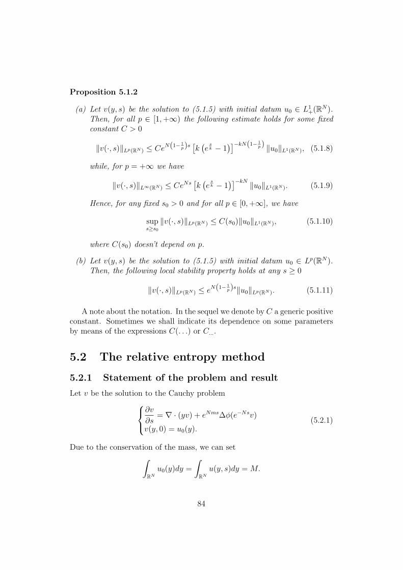
Proposition 5.1.2

(a) Let v(y, s) be the solution to (5.1.5) with initial datum u0 ∈ L1+(RN).

Then, for all p ∈ [1,+∞) the following estimate holds for some fixedconstant C > 0

‖v(·, s)‖Lp(RN ) ≤ CeN(1− 1p)s[k(e

sk − 1

)]−kN(1− 1p) ‖u0‖L1(RN ), (5.1.8)

while, for p = +∞ we have

‖v(·, s)‖L∞(RN ) ≤ CeNs[k(e

sk − 1

)]−kN ‖u0‖L1(RN ). (5.1.9)

Hence, for any fixed s0 > 0 and for all p ∈ [0,+∞], we have

sups≥s0

‖v(·, s)‖Lp(RN ) ≤ C(s0)‖u0‖L1(RN ), (5.1.10)

where C(s0) doesn’t depend on p.

(b) Let v(y, s) be the solution to (5.1.5) with initial datum u0 ∈ Lp(RN).Then, the following local stability property holds at any s ≥ 0

‖v(·, s)‖Lp(RN ) ≤ eN(1− 1p)s‖u0‖Lp(RN ). (5.1.11)

A note about the notation. In the sequel we denote by C a generic positiveconstant. Sometimes we shall indicate its dependence on some parametersby means of the expressions C(. . .) or C....

5.2 The relative entropy method

5.2.1 Statement of the problem and result

Let v be the solution to the Cauchy problem∂v

∂s= ∇ · (yv) + eNms∆φ(e−Nsv)

v(y, 0) = u0(y).(5.2.1)

Due to the conservation of the mass, we can set∫RN

u0(y)dy =

∫RN

u(y, s)dy = M.

84

We expect the solution v(y, s) to behave like the rescaled Barenblatt similar-ity function

v∞(y) =

(CM − λ

|y|2

2

) 1m−1

+

if m 6= 1

CMe− |y|2

2 if m = 1,

(5.2.2)

as s→ +∞, where the constant CM is chosen in such a way that∫RN

v∞(y)dy = M,

and λ depends only on m and on the space dimension N . We emphasizethat v∞ is not a solution to equation (5.2.1). Let us then define our entropyfunctional

H(v) =

1

m− 1

∫RN

v(y)mdy +1

2

∫RN

|y|2v(y)dy if m 6= 1∫RN

v(y) log v(y)dy +1

2

∫RN

|y|2v(y)dy if m = 1.(5.2.3)

Here m is the exponent describing the behaviour of the nonlinearity in zero,given by condition (NL2). We recall that the convex functional H(v) attainsits minimum over L1

+(RN), under the constraint∫

RN v = constant, at thestate v∞ with mass M (see [CT00]). The relative entropy is defined, as usual,by

H (v|v∞) = H(v)−H(v∞).

The above functional H (v|v∞) is related to a Dirichlet–type integral, theso–called entropy production or generalized Fisher information, by means ofthe following Sobolev–type inequality (see [CT00, AMTU00, Gro75]).

Theorem 5.2.1 Let v ∈ L1+(RN) such that

∫RN v(y)dy = M , let v∞ be the

ground state defined in (5.2.2) with mass M . Then, the following inequalityholds,

H(v)−H(v∞) ≤ 1

2I(v|v∞), (5.2.4)

where

I(v|v∞) =

∫RN

v

∣∣∣∣∇( m

m− 1vm−1 +

|y|2

2

)∣∣∣∣2 dy,where m is the same exponent as in the definition (5.2.3) of the entropyfunctional .

85

We also recall the generalized Csiszar–Kullback inequality, which providesan upper bound of the L1 norm of the difference between any positive densityv and the ground state v∞ having the same mass as v, in terms of their relativeentropy. More precisely, we have

Theorem 5.2.2 Let v ∈ L1+(RN), with

∫RN v(y)dy =

∫RN v

∞(y)dy. Then,the following holds

‖v − v∞‖αL1(RN ) ≤ C[H(v)−H(v∞)], (5.2.5)

where

α =

2 if m ≤ 2

m if m ≥ 2,(5.2.6)

where m is again the exponent in the definition (5.2.3) of the entropy func-tional.

In the sequel we shall also need the modified entropy functional (see[BDE02])

E(v, s) = emNs∫

RN

F (e−Nsv)dy +1

2

∫RN

|y|2vdy, (5.2.7)

where

F (u) =

∫ u

0

h(θ)dθ, (5.2.8)

and h is the enthalpy defined in (5.1.7). The function F is well–definedthanks to condition (NL4) in the previous section; moreover, F is everywherenonnegative. We observe that the following identity holds

F (u) = uh(u)− φ(u).

In what follows, we shall assume the solution to enjoy enough regularityin order to be treated as a classical solution; this can be justified, for instance,by supposing that the initial datum u0 is strictly positive. In that case, thesolution u(y, s) is C∞ at any s > 0. The rigorous justification of our resultfor general data then follows by a standard density argument (see [Vaz90]).Let us then state the main result of this section.

Theorem 5.2.3 Let v(y, s) be the solution to the Cauchy problem (5.2.1).Let the initial datum v0 ∈ L1

+(RN) be such that∫RN

F (v0(y))dy +1

2

∫RN

|y|2v0(y)dy +

∫RN

v0(y)mdy < +∞, (5.2.9)

86

where F is defined in (5.2.8). Then, the entropy functional H(v(s)|v∞) sat-isfies

H(v(s)|v∞) ≤ Ce−δs, for all s ≥ 0, (5.2.10)

where δ = min2, N(k + 1), k is the exponent in the structural condition(NL2), and C > 0 is a constant depending on the mass of v0 and on thebounded quantity in (5.2.9).

The Csiszar Kullback inequality (5.2.5) above and the time dependentscaling (5.1.4), then, provides the rate of convergence in L1 for the solutionto the original problem (5.1.1) towards the Barenblatt self–similar functions

u∞(x, t) =

(C − λ

|x|2

t2

N(m−1)+2

) 1m−1

+

. (5.2.11)

Corollary 5.2.4 Let u(x, t) be the solution to the Cauchy problem (5.1.1),with initial datum u0 ≥ 0 such that∫

RN

[um0 (x) + |x|2u0(x) + F (u0(x))

]dx < +∞.

Let u∞(x, t) be the Barenblatt self–similar function given by (5.2.11) with theconstant C such that

∫u∞ =

∫u0. Then, the following estimate holds for all

t ≥ 0‖u(t)− u∞(t)‖L1(RN ) ≤ C(t+ 1)−

λδα , (5.2.12)

where λ is defined in (5.1.4) and α is defined by (5.2.6).

Remark 5.2.5 The hypotesis on the initial data 5.2.9 can be relaxed in casea further assumption on the nonlinearity φ holds, namely φ′(u) ≤ Cum−1 for

some C > 0. This comes by direct computation of the evolution of the secondmoment.

Remark 5.2.6 The rate of convergence in (5.2.12) has been already ob-tained in [BDE02]. However, our result includes more general nonlinearityfunctions. In particular, we don’t need to require the technical condition(m − 1)uh(u) − mf(u) ≤ 0. Moreover, our approach seems to be muchsimpler than that in [BDE02], since we make use the usual nonlinear ver-sion of the Log–Sobolev inequality, and we use directly the Csiszar–Kullbackinequality (5.2.5) in order to get a rate of convergence in L1.

87

5.2.2 Proof of Theorem 5.2.3

In order to prove theorem 5.2.3, we first perform an estimate for large timess, which is obtained basically by means of the regularizing effect (5.1.9) andof the Sobolev–type inequality (5.2.4). Then we use the modified entropyfunctional E defined above in (5.2.7) in order to control the evolution of theentropy in a finite time interval.

Proposition 5.2.7 Under the assumptions (N1)–(N2)–(N3) on the non-linearity φ, there exist an s0 > 0 and a positive constant C(s0) depending ons0 such that, if H(v(s0)) < +∞, then we have

H(v(s)|v∞) ≤ C(s0)e−min2,N(k+1)s. (5.2.13)

Proof. We recall that the equation (5.2.1) can be written in the alternativeway (5.1.6). Then, integration by parts yields

d

dsH(v(s)) =

∫RN

[m

m− 1vm−1 +

|y|2

2

]∇·[v∇(|y|2

2+ eN(m−1)sh(e−Nsv)

)]dy

=−∫

RN

v∇(

m

m− 1vm−1 +

|y|2

2

)·∇(|y|2

2+ eN(m−1)sh(e−Nsv)

)dy.

Hence, we employ the structural condition (NL2) to obtain

d

dsH(v(s)) =−

∫RN

ψ(e−Nsv)

∣∣∣∣∇( m

m− 1vm−1 − |y|2

2

)∣∣∣∣2 dy+−me−Ns

∫RN

v2m−2ψ′(e−Nsv) |∇v|2 dy+

− e−Ns∫

RN

vmψ′(e−Nsv)y · ∇(

m

m− 1vm−1

)dy

=−∫

RN

v

(ψ(e−Nsv)+

1

mψ′(e−Nsv)e−Nsv

)∣∣∣∣∇( m

m− 1vm−1−|y|

2

2

)∣∣∣∣2dy++ eNms

∫RN

(e−Nsv

)mψ′(e−Nsv)y · ∇(e−Nsv)dy+

+1

me−Ns

∫RN

v2ψ′(e−Nsv)|y|2dy =3∑j=1

Ij. (5.2.14)

We first compute the term I2. We observe that, from the hypothesis (P3)on the nonlinearity, the function g(u) = umψ′(u) is is summable over anyinterval [0, L), L > 0. Hence, the primitive

G(u) =

∫ u

0

θmψ′(θ)dθ

88

is well defined on [0,+∞). As a consequence of that, and after integrationby parts, I2 may be written as follows

I2 = −NeNms∫

RN

G(e−Nsv)dy.

Again from the structural hypothesis (P3), it follows easily that G(u) is a(m+k+1)–Holder function on a neighborhood of u = 0. This fact, togetherwith estimate (5.1.9), yields

I2 ≤ C(M, s0)e−N(k+1)s

∫RN

vm+k+1dy

≤ C(M, s0)‖v‖k+1L∞(RN )

e−N(k+1)s

∫RN

vmdy

≤ C(M, s0)e−N(k+1)sH(v(s)),

for some s0 > 0 (chosen in order to have e−Nsv small) and for any s ≥ s0. Ina very similar way, we estimate I3

I3 ≤ C(M, s0)e−N(k+1)

∫RN

v2+k|y|2 ≤ C(M, s0)e−N(k+1)H(v(s)),

for s0 large and s ≥ s0.The integral term I1 may be written as follows.

I1 = −∫

RN

α(s)v

∣∣∣∣∇( m

m− 1vm−1 +

|y|2

2

)∣∣∣∣2 dy,where α(s) = ψ(e−Nsv) + 1

mψ′(e−Nsv)e−Nsv. By means of the structural

condition (NL2) and the first order Taylor expansion, we have

α(s) = 1 + e−Nsvψ′(e−Nsη) +1

me−Nsvψ′(e−Nsv), η ∈ [0, v(s)].

We employ once again the regularizing effect (5.1.9) to get

α(s) ≥ 1− C(M, s0)e−N(k+1)s, s ≥ s0,

and we can choose s0 large enough in order to have α(s) ≥ 0 for any s ≥ s0.Hence, we put the above estimates into (5.2.14) and we use the Sobolev–typeinequality (5.2.4) to recover

d

dsH(v(s)|v∞) ≤ −2

(1− C(M, s0)e

−N(k+1))H(v(s)|v∞)+

+ C(M, s0)e−N(k+1)sH(v(s))

≤ −2(1− C(M, s0)e

−N(k+1))H(v(s)|v∞)+

+ C(M, s0)e−N(k+1)sH(v∞).

89

Finally, we use the variation of constants formula and obtain the desiredestimate (5.2.13).

We now perform a local–in–time estimate of the entropy, in order tocontrol the constant C(s0) in the inequality (5.2.13).

Lemma 5.2.8 Suppose that the initial datum u0 satisfies (5.2.9). Then, thefollowing inequality holds at any s ≥ 0,

E(v(s)) ≤ e(m−1)sE(v0), (5.2.15)

where E(u) is defined in (5.2.7). In particular, the entropy H(v(s)) is uni-formly bounded on any finite time interval [0, s0].

Proof. We calculate the evolution in time of the functional E(v(s), s)defined in (5.2.7) (see [BDE02]). After integration by parts, we get

d

dsE(v(s)) = −

∫RN

v∣∣y + e(m−1)Ns∇h(e−Nsv)

∣∣2 dy++ emNs

∫RN

[(m− 1)ve−Nsh(e−Nsv)−mφ(e−Nsv)

]dy

≤ emNs(m− 1)

∫F (e−Nsv)dy ≤ (m− 1)E(v(s)),

which proves (5.2.15). The last assertion comes directly from (5.1.11).

Remark 5.2.9 The entropy dissipation method has been successfully usedin [CF03] in order to prove convergence towards Barenblatt solutions fordiffusion dominated convection–diffusion equations. By means of the sameapproach in the present chapter, one can generalized the results in [CF03] toa generalized convection–diffusion model where the power law in the diffusionterm is replaced by a more general φ satisfying the hypothesis above.

5.3 Evolution of the 1-d Wasserstein distances

5.3.1 Preliminaries and results

In this section we analyze the Cauchy problem (5.1.1) in one space dimension,i.e.

ut = φ(u)xx

u(x, 0) = u0(x),(5.3.1)

where the initial datum u0 is taken in L1+(R).

90

We require the nonlinearity function φ to satisfy the conditions (NL1)and (NL2) stated at the beginning of section 5.1. To simplify the calculationsbelow, we can express condition (NL2) in the following alternative way

(NL2) φ(u) = um+ψ(u), where ψ(u) = O(un) as u→ 0, for some n > m,ψ ∈ C1((0,+∞)).

Moreover, we restrict ourselves to the slow diffusion cases by requiring

(SD) φ′(0) = 0 iff m > 1.

As in the previous section, we perform the time dependent scaling (5.1.4),which turns equation (5.3.1) into

vs = (yv + emsφ(e−sv)y)yv(y, 0) = u0(y).

(5.3.2)

In the sequel we shall assume for simplicity that∫ +∞−∞ u0(x)dx = 1. Our

aim is to study, for any p ∈ [1,+∞], the dynamic induced by the aboveequation (5.3.2) on the metric space

M2p = U(·) ∈ L1+(R),

∫ +∞

−∞|x|2pu(x)dx <∞

endowed with the p–Wasserstein distance

W2p(U, V ) = inf

[∫ +∞

−∞|x− Tx|2pU(x)dx

] 12p

, (5.3.3)

where the infimum is taken over the admissible maps T : R → R such that∫ +∞

−∞ψ(x)V (x)dx =

∫ +∞

−∞ψ(Tx)U(x)dx, for all ψ ∈ C0(R). (5.3.4)

The condition (5.3.4) is often referred as T being a push–forward of themeasure Udx onto the measure V dx (notation: V = T]U).

The precise definition of the Wasserstein distances comes from a relaxedvariational problem, the so–called Monge–Kantorowich mass transportationproblem. More precisely, the set of admissible maps defined in (5.3.4) isembedded into the set of all probability measures π on R2 with marginalsgiven by Udx and V dx. The cost defined in the definition (5.3.3) is thenconverted into [∫ ∫

R2

(x− y)2pµ(dx, dy)

] 12p

.

91

It has been proved (in a much more general context! See [Vil03] and thereferences therein), that the optimal measure π∗, which minimizes the relaxedvariational problem, is supported on the graph of a map T ∗ : R → R. Hence,the infimum in (5.3.3) is actually a minimum. We refer to [Vil03] for adetailed explanation of these topics. For further reference, we only recall theproperty

p ≤ q ⇒ W2p(U, V ) ≤ W2q(U, V ). (5.3.5)

In one space dimension, the optimal mat T ∗ can be expressed in a very simpleway (see also [CT03, CGT03]). Given two probability measures Udx, V dx ∈M2p, we define the distribution functions

F (x) =

∫ x

−∞U(y)dy G(x) =

∫ x

−∞V (y)dy,

and their pseudo–inverses F−1, G−1 : [0, 1] → R

F−1(ρ) = infω : F (ω) > ρ G−1(ρ) = infω : G(ω) > ρ

(eventually F−1 and G−1 may attain the values ±∞ at ρ = 0 or at ρ = 1).Then, it can be easily proved that the optimal map T ∗ between Udx andV dx is

T ∗ = G−1 F.

Hence, by writing down the definition (5.3.3) of Wasserstein distance in termsof the optimal T ∗, and after a change of variable, we get

W2p(U, V ) =

[∫ 1

0

∣∣F−1(ρ)−G−1(ρ)∣∣2p dρ] 1

2p

. (5.3.6)

Thanks to the monotonicity property (5.3.5), one can eventually send p→∞to obtain

W∞(U, V ) = supρ∈(0,1)

∣∣F−1(ρ)−G−1(ρ)∣∣

One can easily see that, whenever U and V have compact support, the abovequantity W∞(U, V ) controls the ‘distance’ between the supports of U and Vrespectively. More precisely, we have (see [CT03])

|infsupp U − infsupp V | ≤W∞(U, V )

|supsupp U − supsupp V | ≤W∞(U, V ) (5.3.7)

Let us now turn back to the rescaled equation (5.3.2). From the results inthe previous section, we already know (in some sense), that the evolution of

92

the solution v for large s is dominated by the power nonlinearity um. Thus,we also expect that the Wasserstein distance between the solution v(·, s) ofequation (5.3.2) and the corresponding Barenblatt profile v∞ with mass 1(defined in (5.2.11)) tends to zero as s goes to +∞. In order to study theevolution of such a quantity, because of all the above observations about theone–dimensional case, we set

F (y, s) =

∫ y

−∞v(z, s)dz

G(y, s) =

∫ y

−∞v∞(z)dz.

Let F−1, G−1 : (0, 1) → R be the pseudo–inverses of F and G respectively.Then, F−1 satisfies the following equation (similar computations can be foundin [CT03, CGT03]),

∂F−1

∂s= −F−1 − ∂

∂ρ

[∂F−1

∂ρ

]−m+ emsψ

(e−s(∂F−1

∂ρ

)−1)

, (5.3.8)

while G−1 satisfies

G−1 +∂

∂ρ

[(∂G−1

∂ρ

)−m]= 0. (5.3.9)

We next state our result concerning Wasserstein distances.

Theorem 5.3.1 Let φ(u) satisfy conditions (NL1), (NL2), and (SD)above.

(a) Let v(y, s) be the solution to (5.3.2) with u0 ∈ L1+(R) having mass 1

and finite second moment. Let v∞ be the rescaled Barenblatt profilewith mass 1 defined by (5.2.2). Then, for any p ≥ 1, the followingholds

W2p(v(s), v∞) =

[∫ 1

0

∣∣F−1(ρ)−G−1(ρ)∣∣2p dρ] 1

2p

≤ Ce−s, (5.3.10)

where C = C0 +W2p(u0, v∞) and C0 depends only on φ.

(b) Let v(y, s) be the solution to (5.3.2) with u0 ∈ L1+(R) having mass 1

and compact support. Let v∞ be the rescaled Barenblatt profile withmass 1 defined by (5.2.2). Then

W∞(v(s), v∞) ≤ Ce−s, (5.3.11)

where C = C0 +W∞(u0, v∞) and C0 depends only on φ.

93

In the original variables (5.3.1), the part (b) of the previous theoremprovides our result concerning with the speed of propagation of the supportof any solution u(x, t) having compactly supported initial datum u0. Indeed,

since the support of the Barenblatt profile is a ball of radius C(t+ 1)1

m+1 forsome fixed constant C > 0, we easily obtain the following result.

Corollary 5.3.2 Let u(x, t) be the solution to (5.3.1) with u0 ∈ L1+(R) hav-

ing compact support. Then, there exist two positive constants C1 < C2 suchthat

|infsupp u(t) − infsupp u∞(t)| ≤ C1

|supsupp u(t) − supsupp u∞(t)| ≤ C2 (5.3.12)

Remark 5.3.3 We found a lot of references in the literature concerning thefinite speed of propagation property in slow diffusion equations (see [Kne77,Kal87] for the general nonlinear case). Most of them are based on heavyanalytic tools. Our result is more complete in general nonlinear case, andcovers a wide class of nonlinearities. Moreover, our technique seems to beapplied to this problem in a very natural way.

5.3.2 Proof of Theorem 5.3.1

To perform the proof of theorem 5.3.1, we compute the evolution of theWasserstein distance W2p(v(s), v

∞) by means of the one–dimensional repre-sentation formula (5.3.6). The calculations below are formal, in the sensethat we should need the pseudo–inverse function F−1 to be smooth enough.We observe that this occurs when the initial datum u0 is supported on ainterval. We could make this argument rigorous by means of standard ap-proximation tools (see [CGT03]). We skip these details and suppose thatF−1 is smooth. Moreover, we need to know a priori that the speed of propa-gation of the support of the solution is finite. This property, which actuallycharacterizes slow diffusion equations, was proved by Kalashnikov, Oleinikand Yiu–Lin (see [Kal87] and the references therein). Using the notations ofthe previous subsection, thanks to (5.3.9) and after integration by parts, we

94

have

d

ds

∫ 1

0

[F−1 −G−1

]2pdρ = 2p

∫ 1

0

[F−1 −G−1

]2p−1 ∂

∂sF−1(ρ, s)dρ

= 2p

∫ 1

0

[F−1 −G−1

]2p−1

[−F−1− ∂

∂ρ

((∂F−1

∂ρ

)−m+ emsψ

(e−s(∂F−1

∂ρ

)−1))

+

+G−1 +∂

∂ρ

((∂G−1

∂ρ

)−m)]

= −2p

∫ 1

0

[F−1 −G−1

]2pdρ− 2p(2p− 1)

∫ 1

0

[F−1 −G−1

]2p−2(∂F−1

∂ρ−∂G

−1

∂ρ

)×

× ems

[φ

(e−s(∂F−1

∂ρ

)−1)− φ

(e−s(∂G−1

∂ρ

)−1)]

dρ

− 2p

∫ 1

0

[F−1 −G−1

]2p−1 ∂

∂ρ

(emsψ

(e−s(∂G−1

∂ρ, s

)−1))

. (5.3.13)

We observe that, due to the compact support of the solutions, the boundaryterm coming from integration by parts disappears (see [CT03, CGT03]). Infact, this boundary term is given by

∑i=0,1

(−1)i2p[F−1(i, s)−G−1(i)

]2p−1

[(∂F−1

∂ρ

)−m(i, s)+

emsψ

(e−s(∂F−1

∂ρ

)−1)

(i, s)−(∂G−1

∂ρ

)−m(i, s)

].

The first bracket is bounded at any s because of the finite speed of prop-agation property of the solutions. The second bracket is a sum of positivepowers of the solution v and of the Barenblatt function v∞ evaluated at theboundary of their support respectively. Hence, this second bracket equalszero.

Now, since the function φ is increasing, the second integral at the end of(5.3.13) is nonnegative. This observation is the key point in this computation(see again [CGT03]). In fact, thanks to this we can get rid of the nonlinearityterm, and we have only to estimate the term depending on the Barenblattprofile, which is known. Indeed, after some calculations in the very last term

95

of (5.3.13), due to (5.3.9), we obtain the following inequality

d

ds

∫ 1

0

[F−1 −G−1

]2pdρ ≤ −2p

∫ 1

0

[F−1 −G−1

]2pdρ

− 2p

me(m−1)s

∫ 1

0

[F−1 −G−1

]2p−1G−1ψ′

(e−s(∂G−1

∂ρ

)−1)(

∂G−1

∂ρ

)m−1

dρ.

Because of the condition (NL2) on ψ, we can assume that ψ(u) = ung(u),with g′(u) = O(uk), k > −1, as u → 0. Then, it follows that ψ′(u) =O(un−1), as u → 0. Hence, thanks to Holder inequality, the last integralabove can be estimated from above by the term

C(v∞)pe−(n−m)s

(∫ 1

0

∣∣F−1 −G−1∣∣2p−1

dρ

) 2p−12p

,

where the constants C(v∞) is given by

C(v∞) = ‖v∞‖L∞(R) max| infsupp v∞|, | supsupp v∞|

(this quantity depends only on the mass and on the exponent m). We nowapply the variation of constants formula in order to get the rate of conver-gence to zero of Wp(v(s), v

∞). In order to perform this task, we set forsimplicity

Xp(s) =

∫ 1

0

[F−1(ρ, s)−G−1(ρ)

]2pdρ.

Hereafter, C denotes a fixed positive constant independent on p and s. Sofar we have proved that

d

dsXp(s) ≤ −2p Xp(s) + 2p Ce−(n−m)sXp(s)

2p−12p . (5.3.14)

By Young inequality we get

d

dsXp(s) ≤ −2p

(1− Ce−(n−m)s

)Xp(s) + Ce−(n−m)s.

In a similar fashion to the computation of the entropy in the previous section,by means of the variation of constants formula we easily obtain

Xp(s) ≤ (Xp(0) + C) e−min2p,(n−m)s. (5.3.15)

In case that n − m < 2p, the exponential rate of convergence in (5.3.15)can be improved iteratively by substituting the above inequality in the lastaddend of (5.3.14), until it reaches the value e−2ps. Obviously, the number ofsteps depends on p. We have thus proved (5.3.10). The inequality (5.3.11),then, easily follows by sending p→∞.

96

Remark 5.3.4 It is worth to remark that in the above computation wedon’t need the hypothesis (NL3) on the nonlinearity, since we don’t needthe apriori estimates (5.1.8)–(5.1.9) on the solution v (which are consequencesof the L1–L∞ regularizing effect), which was one the tools in the proof of theentropy dissipation result in the previous section.

97

Chapter 6

A small perturbation result fornonlinear diffusion far fromvacuum

This chapter contains a stability under small perturbation result for theporous medium equation far from vacuum.

6.1 Statement of the problem and result

In this chapter we prove the asymptotic stability of certain caloric self–similarsolutions to the generalized porous medium equation

ρt = p(ρ)xx, (6.1.1)

where the pressure p is smooth and strictly increasing. By caloric self–similarsolutions we mean a class of similarity solutions of the form

ρ(x, t) = f

(x2

t+ 1

)satisfying the limiting conditions

ρ(±∞, t) = ρ±,

for strictly positive ρ+, ρ−. For the existence of such solutions we refer to[AP71, AP74, vDP77, vDP77]. We recall here that for the caloric profile ρ

98

the following estimates hold∣∣∣∣∂α+β ρ(t)

∂xα∂tβ

∣∣∣∣∞

=O(δ)1

(t+ 1)α2+β

α, β > 0∫ +∞

−∞

∣∣∣∣∂α+β ρ(x, t)

∂xα∂tβ

∣∣∣∣2dx =O(δ2)1

(t+ 1)α+2β− 12

α, β > 0, (6.1.2)

where δ = |ρ+ − ρ−|. Let us denote by ρ the solution to the same equation(6.1.1) with the same limiting conditions at infinity and with the initial datumgiven by a small perturbation of ρ(x, 0). Let us denote

r(x, t) = ρ(x, t)− ρ(x+ x0, t),

where x0 will be determined later on. By integrating w.r.t. x the equationsatisfied by r, we get

d

dt

∫ +∞

−∞r(x, t)dx =

[p(ρ(x, t))− p(ρ(x+ x0, t))

]x

∣∣∣∣+∞−∞

= 0 ,

Thus, if one has ∫ +∞

−∞

[ρ0(x)− ρ0(x+ x0)

]dx = 0 ,

it follows both

x0 =1

ρ+ − ρ−

∫ +∞

−∞[ρ0(x)− ρ0(x)] dx (6.1.3)

and ∫ +∞

−∞r(x, t)dx = 0.

Let us define the primitive variable

R(x, t) =

∫ x

−∞r(ξ, t)dξ , (6.1.4)

which satisfies the following problemRt = p(ρ+Rx)x − p(ρ)x

R(x, 0) =

∫ x

−∞[ρ0(ξ)− ρ0(ξ + x0)]dξ

R(±∞, t) = 0.

(6.1.5)

Then, the small perturbation analysis with respect to the caloric self-similarsolution is given by the following result.

99

Theorem 6.1.1 Let us suppose that ‖R(0)‖25 is sufficiently small. Then, for

any t ≥ 0, we have

5∑k=0

(t+ 1)k‖R(k)(t)‖2 +

∫ t

0

(τ + 1)k‖R(k+1)(τ)‖2dτ ≤ C‖R(0)‖25. (6.1.6)

The proof of the Theorem (6.1.1) will be given in the next section.

6.2 The Proof of the Theorem 6.1.1

In this section we proof the asymptotic stability result (6.1.6) by means of acontinuation principle. We start with the a priori condition

sup0≤t≤T

5∑k=0

(1 + t)k‖R(k)(t)‖2 ≤ σ. (6.2.1)

Lemma 6.2.1 Suppose σ 1. Then

‖R(t)‖2 +

∫ t

0

‖Rx(s)‖2ds ≤ O(1)‖R0‖2. (6.2.2)

Proof. By multiplying the first equation in (6.1.5) by R and after integra-tion over R, we get

d

dt

1

2‖R(t)‖2 =

∫ +∞

−∞[p(ρ+Rx)x − p(ρ)x]Rdx =

=−∫ +∞

−∞[p(ρ+Rx)− p(ρ)]Rxdx =

=−∫ +∞

−∞

[p′(ρ)R2

x +R1(p, ρ, Rx)Rx

]dx ≤

≤−O(1)‖Rx(t)‖2 +O(σ)‖Rx(t)‖2.

We denoted by R1(p, ρ, Rx) the remainder in the first order Taylor expansionof p′ around ρ. The last inequality is due to the uniform boundedness of thecoefficient p′′(ζ) when ζ ∈ (ρ, ρ + Rx) (as a consequence of the maximumprinciple). Then, we integrate over [0, t] and get the desired estimate (6.2.2).

Lemma 6.2.2 Suppose σ 1. Then we have

(1 + t)‖r(t)‖2 +

∫ t

0

(1 + s)‖rx(s)‖2ds ≤ O(1)‖R0‖21. (6.2.3)

100

Proof. By differentiating the equation (6.1.5) w.r.t. x, we get

rt =p(ρ)xx − p(ρ)xx = (p′(ρ)ρx − p′(ρ)ρx)x =

= [p′(ρ)rx + (p′(ρ)− p′(ρ)) ρx]x . (6.2.4)

We multiply (6.2.4) by (1 + t)r and integrate over R to obtain

d

dt

[(1 + t)

‖r(t)‖2

2

]− ‖r(t)‖2 =

=(1 + t)

∫ +∞

−∞(p′(ρ)rx)x rdx+ (1 + t)

∫ +∞

−∞((p′(ρ)− p′(ρ)) ρx)x rdx

=− (1 + t)

∫ +∞

−∞p′(ρ)r2

xdx− (1 + t)

∫ +∞

−∞(p′(ρ)− p′(ρ)) ρxrxdx.

Finally, by integrating w.r.t. to time, we get

(1 + t)1

2‖r(t)‖2 +

∫ t

0

(1 + s)‖rx(s)‖2ds ≤ O(1)‖r(0)‖2+

+O(1)

∫ t

0

‖r(s)‖2ds+O(δ)

∫ t

0

(1 + s)1/2‖r(s)‖‖rx(s)‖ds ≤

≤O(1)‖R(0)‖21 +O(1)

∫ t

0

[‖r(s)‖2 +O(δ)(1 + s)‖rx(s)‖2

]ds ≤

≤O(1)‖R(0)‖21 +O(δ)

∫ t

0

(1 + s)‖rx(s)‖2ds,

where we have used (6.1.2) and Lemma 6.2.1. Thus, for δ 1, we have thedesired estimate (6.2.3).

Let us write the equation satisfied by rx:

rxt = (p′(ρ)ρx − p′(ρ)ρx)xx . (6.2.5)

Hence, we obtain the following Lemma.

Lemma 6.2.3 Let σ 1. Then

(1 + t)2‖rx(t)‖2 +

∫ t

0

(1 + s)2‖rxx(s)‖2ds ≤ O(1)‖R(0)‖22. (6.2.6)

Proof. From (6.2.5) we have

rxt − (p′(ρ)rx)xx = [(p′(ρ)− p′(ρ)) ρx]xx .

101

We multiply by (1 + t)2rx and integrate over R to get

d

dt

[(1 + t)2 1

2‖rx(t)‖2

]− (1 + t)‖rx(t)‖2

+(1 + t)2

∫ +∞

−∞p′(ρ)r2

xxdx = −(1 + t)2

∫ +∞

−∞[p′′(ρ)ρxrxrxx

+ (p′(ρ)− p′(ρ)) ρxxrxx + (p′(ρ)− p′(ρ))x ρxrxx] dx.

Then, by integrating w.r.t. time, we obtain

(1 + t)2‖rx(t)‖2 +

∫ t

0

(1 + s)2‖rxx(s)‖2ds ≤

≤O(1)‖rx(0)‖2 +O(1)

∫ t

0

(1 + s)‖rx(s)‖2ds

+O(1)

∫ t

0

(1 + s)2

∫ +∞

−∞

[r2xrxx + ρxrxrxx + rrxxρxx

+ rxρxrxx + rρ2xrxx

]dxds ≤ O(1)‖R(0)‖2

2

+O(1)

∫ t

0

(1 + s)1/2|rx(s)|∞[(1 + s)‖rx(s)‖2 + (1 + s)2‖rxx(s)‖2

]ds

+O(δ)

∫ t

0

[(1 + s)‖rx(s)‖2 + (1 + s)2‖rxx(s)‖2

+ ‖r(s)‖2 + (1 + s)2‖rxx(s)‖2 +O(δ)(1 + s)‖rxx(s)‖2]ds,

where we have used Young inequality. Thus, using (6.2.1), (6.2.2) and (6.2.3),together with δ 1, we get

(1 + t)2‖rx(t)‖2 +

∫ t

0

(1 + s)2‖rxx(s)‖2ds ≤ O(1)‖R(0)‖22+

+O(σ)

∫ t

0

[(1 + s)2‖rxx(s)‖2 + (1 + s)‖rx(s)‖2

]ds.

Finally, by means of (6.2.3) and since σ 1, we get the desired result(6.2.6).

In order to complete the energy estimate (6.1.6) we have to carry out thetime dacay estimates for the higher order derivatives rxx, rxxx, rxxxx, , whichcan be done by following the same technique as above. We omit the detailsabout this calculations.

102

Chapter 7

The viscous Burgers Equation

This chapter has to do with the classical viscous Burgers’ equation describedin section 1.8 of the introduction. We use the entropy dissipation approachto recover optimal rates of convergence towards diffusive waves. In the nextsection 7.1 we show how this equation inherits the gradient flow structureof the heat equation (cfr. section 1.7) by means of the famous Hopf–Coletransformation. Section 7.2 is devoted to the statement and the proof of theresults concerning with the relative entropy approach. In the last section weprove a simple stability result for the 2–Wasserstein distance.

7.1 The Hopf–Cole Transformation

The time–asymptotic analysis for the viscous Burgers’ equation

ut + uux = uxx, (7.1.1)

is based on the classical Hopf–Cole transformation, which reduces (7.1.1) tothe linear heat equation. In this section, we first explain the classical processused to obtain the typical intermediate–asymptotic states for this equation(see [Hop50]). Afterwards, we set up a different framework of notations, inorder to convert (7.1.1) into the linear Fokker–Planck equation.

7.1.1 The classical setting

We consider the initial value problemut +

(u2

2

)x

= uxx

u(x, 0) = u0(x)(7.1.2)

103

where x ∈ R, t > 0, u ∈ R and u0 is a given function in L1(R). It is wellknown (see [Hop50]) that, if u(·, t) is the solution of (7.1.2) at a positive timet, then the following conservation property holds∫ +∞

−∞u(x, t)dx =

∫ +∞

−∞u0(x)dx.

We denote in the following ∫ +∞

−∞u0(x)dx = M. (7.1.3)

The unique solution of (7.1.2) can found explicitely by means of the Hopf–Cole tranformation

φ(x, t) = exp

(−1

2

∫ x

−∞u(y, t)dy

)u(x, t) = −2

φx(x, t)

φ(x, t), (7.1.4)

which reduces (7.1.2) to the linear heat equation φt = φxx. Indeed, via theconvolution formula for the heat equation, one obtains

u(x, t) =

∫ +∞−∞

x−yte−

|x−y|22t

−∫ y−∞ u0(z)dxdy∫ +∞

−∞ e−|x−y|2

2t−

∫ y−∞ u0(z)dxdy

. (7.1.5)

Moreover, one can construct a diffusion wave type solution UM for (7.1.2)with mass M , corresponding to the solution

ΦM(x, t) = 1− CM

∫ x(2t+1)−1/2

−∞e−

ζ2

2 dζ (7.1.6)

of the heat equation. The costant CM in the above formula is determined inorder to match condition (7.1.3).

To construct ΦM , we observe that the spatial derivative z(x, t) = −φx(x, t)(φ given by (7.1.4)) satisfies again the heat equation zt = zxx and it has aninitial datum z0 ∈ L1(R). Hence, one can consider the gaussian solution ofthe heat equation with the same mass as z0, namely

ZM(x, t) = CM(2t+ 1)−1/2e−x2

2(2t+1) , (7.1.7)

and write the corresponding ΦM by taking the spatial primitive of ZM (thelimiting conditions for Φ are determined by the conservation of mass). Fi-nally, by replacing φ with ΦM into (7.1.4), one obtains the diffusion wave

UM(x, t) = 2CM(2t+ 1)−12

exp(− x2

2(2t+1)

)1− CM

∫ x(2t+1)−1/2

−∞ e−ζ2

2 dζ. (7.1.8)

104

7.1.2 Intermediate asymptotics and zero–viscosityregime

Let us consider equation (7.1.1) with a small viscosity parameter µ > 0, i. e.ut +

(u2

2

)x

= µuxx

u(x, 0) = u0(x),(7.1.9)

with initial datum u0 ∈ L1(R) eventually sign–changing. In the limit asµ → 0, one recovers the unique entropy solution of the Cauchy problem forthe inviscid Burgers’ equation

ut +(u2

2

)x

= 0

u(x, 0) = u0(x).(7.1.10)

It is well–known that the quantities

p = − infx∈R

∫ x

−∞u0(y)dy q = sup

x∈R

∫ +∞

x

u0(y)dy

are invariant for equation (7.1.10). Hence one can construct the N–wavetype solution

Np,q(x, t) =

xt

if −√

2pt ≤ x ≤√

2qt

0 otherwise,(7.1.11)

which turns out to be the an attractor in the L1 norm for any solutionof (7.1.10) with initial datum having compact support and negative andpositive masses given by p and q respectively (see [Lax57, DP75]). In case ofnonnegative data with mass M , (7.1.11) becomes

NM(x, t) =

xt

if 0 ≤ x ≤√

2Mt

0 otherwise.(7.1.12)

As we pointed out before, in the case of a nonnegative initial datum u0 for theviscous Burgers’ equation (7.1.2), the mass M =

∫u0 is the only information

needed to construct the asymptotic diffusive wave UM given in (7.1.8). Withthe small viscosity parameter µ as in (7.1.9), this solution becomes

UM,µ(x, t) = 2µCM,µ(2t+ 1)−12

exp(− x2

2µ(2t+1)

)1− CM,µ

∫ x(2t+1)−1/2

−∞ e−ζ2

2µdζ, (7.1.13)

105

with CM,µ = 1 − e−12µ . It can be easily checked that, for any fixed (x, t) ∈

R× R+,UM,µ(x, t) −→ NM(x, t+ 1/2) as µ→ 0,

where NM is given by (7.1.12), that is, the diffusive wave UM,µ approximatesa positive N–wave in the zero–viscosity limit. As pointed out by T.P. Liu inhis introduction to [Liu85], this situation is an example of how the behaviorof a nonlinear conservation law, at the level of diffusion waves, changes con-siderably with the presence of the viscosity (even when this is small). In thecase the of Burgers’ equation, an intermediate state for the viscous case (forgeneral possibly sign-changing initial data) is provided by

U(x, t) = −2µφ(x, t)

1−∫ x−∞ φ(y, t)dy

, (7.1.14)

where

φ(x, t) =a√

2πµte−

x2

2µt − b√2πµt

e−x2

2µt

and

a =1

2µ

∫ +∞

−∞u−0 (y)e−

12µ

∫ y−∞u0(z)dzdy b =

1

2µ

∫ +∞

−∞u+

0 (y)e−12µ

∫ y−∞u0(z)dzdy.

For fixed (x, t), the function U tends to the N–wave defined in (7.1.11) asµ tends to zero. The very interesting paper by Kim and Tzavaras ([KT01])provides a quantitative understanding of the long–time–small–viscosity in-terplay for the Burgers’ equation. It turns out that that, when the viscosityis fixed small, at a first asymptotic stage the solution tends to take the shapeof an approximate N–wave of the type (7.1.14) (thus, its behavior is mainlygoverned by convection). Then, at a very long time stage, the diffusion pro-duces an interaction between the positive and the negative masses, and thesmallest between them is consumed, while the profile of the solution tendsto that of the diffusive wave UM defined in (7.1.13).

In the present chapter we do not deal with the zero viscosity limit, eventhough an interesting problem could be the understanding of the limitingbehavior of the estimates carried out in our work as µ approaches to zero.

We also mention that the entropy approach for the inviscid Burgers’ equa-tion has been recently used by Dolbeault and Escobedo in [DE], where the au-thors use a time–dependent scaling in order to view the N–wave type solutionas a stationary state. The convergence towards equilibrium is then provenby means of an entropy functional which provides a decay in a weightedL1–norm.

106

7.1.3 The time–dependent scaling

We are now interested in the study of the asymptotic convergence of thesolution u of (7.1.2) towards UM given by (7.1.8) as t→∞. To perform thistask, we consider a time-dependent scaling which transforms this problemof the study of the asymptotic stability of a stationary state. This idea hasbeen frequently employed in the study of the time–asymptotics for nonlineardiffusion equations (see, for instance, the pioneering paper by Barenblatt[Bar52]). More precisely, we set

y = y(x, t) = xR(t)−1

s = s(t) = logR(t) (7.1.15)

u(x, t) = R(t)−1ρ(y(x, t), s(t)),

whereR(t) = (2t+ 1)1/2.

With this notation, (7.1.2) turns into the following Cauchy problem for theBurgers–Fokker–Plank equation

∂ρ

∂s=

∂

∂y

(∂ρ

∂y+ yρ− ρ2

2

)ρ(y, 0) = ρ0(y) = u0(y).

(7.1.16)

The equation (7.1.16) is often referred to as the viscous Burgers’ equation insimilarity variables. Obviously, we have again the conservation of the mass∫ +∞

−∞ρ(y, s)dy =

∫ +∞

−∞ρ0(y)dy = M.

To recover the suitable stationary solution with mass M of (7.1.16), we em-ploy once again the Hopf–Cole transformation

τ(y, s) = exp

(−1

2

∫ y

−∞ρ(ζ, s)dζ

), (7.1.17)

which converts (7.1.16) into

∂τ

∂s=∂2τ

∂y2+ y

∂τ

∂y.

Hence, the spatial derivative

ψ(y, s) = −∂τ∂y

(y, s) =1

2ρ(y, s) exp

(−1

2

∫ y

−∞ρ(ζ, s)dζ

)(7.1.18)

107

satisfies the Cauchy problem for the linear Fokker–Planck equation∂ψ

∂s=

∂

∂y

(∂ψ

∂y+ yψ

)ψ(y, 0) = ψ0(y) = 1

2ρ0(y) exp

(−1

2

∫ y−∞ ρ0(ζ)dζ

).

(7.1.19)

The inverse transformation of (7.1.18) is given by

ρ(y, s) = −2ψ(y, s)

1−∫ y−∞ ψ(ζ, s)dζ

. (7.1.20)

An easy computation gives∫ +∞

−∞ψ0(y)dy = −

∫ +∞

−∞

∂

∂y

(exp

(−1

2

∫ y

−∞ρ0(ζ)dζ

))dy = 1− e−

M2 =: m.

Hence, conservation of the total mass for the Fokker–Planck equation (7.1.19),implies ∫ +∞

−∞ψ(y, s)dy = m

for any s > 0. It is well known that (7.1.19) has the unique Gaussianequilibrium Ψm with mass m, namely

Ψm(y) =m√2πe−

y2

2 . (7.1.21)

By putting Ψm into (7.1.20), we recover our steady state for the Burgers–Fokker–Planck equation (7.1.16)

ρ∞M(y) =

2m√2πe−

y2

2

1− 2m√2π

∫ y−∞ e−

ζ2

2 dζ. (7.1.22)

By returning back to the original variables x, t, u, it turns out that the sta-tionary state ρ∞M corresponds precisely to the diffusion wave UM defined in(7.1.8).

We close this section by recalling an easy estimate for the function τ(y, t),defined by the Hopf–Cole transformation (7.1.17), which will be useful in thesequel. Since the initial datum for the original Burgers’ equation u0 belongsin L1(R), the quantities

p = − infx∈R

∫ x

−∞u0(y)dy (7.1.23)

q = supx∈R

∫ +∞

x

u0(y)dy = M + p

108

are then finite. In terms of τ , relations (7.1.23) provide the following propertyfor τ(·, 0)

e−(M+p)

2 ≤ τ(y, 0) ≤ ep2 ,

for any y ∈ R. Hence, by simple maximum principle, we obtain the estimate

e−(M+p)

2 ≤ τ(y, t) ≤ ep2 , (7.1.24)

for all (y, t) ∈ R× R+.As it was first proved by Hopf ([Hop50]), the large time behavior of so-

lutions of the original problem (7.1.2) is described by the diffusion wave UMdefined by (7.1.8). Our purpose here is to investigate the large time behaviorof u(x, t) in terms of solutions of equation (7.1.16). Hence, hereafter we shalldiscuss the asymptotic stability of the stationary solution ρ∞M of equation(7.1.16).

7.2 Trend to equilibrium in relative entropy

In this section we analyze the convergence towards the stationary profile ρ∞Mdefined by (7.1.22) for the solution ρ of equation (7.1.16) with initial datumρ0 ∈ L1(R). We start by treating the case of non–negative initial data u0.The general case will be covered later on. Our choice of the functionals usedto control the distance between u and u are the relative entropy functionals

He(ρ(s)|ρ∞M) =

∫ +∞

−∞e

(ρ(y, s)

ρ∞M(y)

)ρ∞M(y)dy, (7.2.1)

where e : R+ → R+ is a smooth function satisfying the following conditions

e(1) = 0

e′′(h) ≥ 0 for any h ∈ R+, e′′ not identically 0

(e′′′)2 ≤ 1

2e′′e(IV ). (7.2.2)

Such functions are called entropy generating functions, and the correspondingfunctionals He are called admissible relative entropies (see [AMTU01]). Inparticular, one can prove that functions e satisfying the above conditionsare strictly convex. Moreover, since ρ and ρ∞m have the same mass, we canobtain the same functional He by “normalizing” the generating function e insuch a way that e′(1) = 0. As a consequence of the above conditions, eachgenerating function satisfies (see [AMTU01], Lemma 2.6)

χ(h) ≤ e(h) ≤ ϕ(h), (7.2.3)

109

where we have denoted

χ(h) = α(h+ β) logh+ β

1 + β− α(h− 1), ϕ(h) = µ2(h− 1)2,

with µ2, α, β nonnegative constants depending on e′′(1) and e′′′(1), namely

µ2 = e′′(1), α = −e′′(1)2

e′′′(1), β = −e

′′(1) + e′′′(1)

e′′′(1). (7.2.4)

The constants (7.2.4) are well defined if e′′′(1) 6= 0. In the case e′′′(1) = 0, onehas to set χ(h) = µ2

2(h−1)2. Hence, the admissible relative entropy approach

allows us to cover a large range of functionals, including the physical relativeentropy

∫ρ log ρ

ρ∞mdx. We refer to [AMTU01] for a detailed explanation of

the mathematical properties of the relative entropies and their generatingfunctions.

By means of so–called Csiszar–Kullback inequalities, one can control theL1 norm of the difference ρ− ρ∞M in terms of the relative entropy functionalsdefined in (7.2.1).

Theorem 7.2.1 (Csiszar–Kullback) There exists a positive constant Csuch that, for all functions ρ1, ρ2 ∈ L1

+(R), with∫Rρ1(x)dx =

∫Rρ2(x)dx (7.2.5)

and for all admissible generating functions e, we have

‖ρ1 − ρ2‖2L1(R) ≤ CHe(ρ1|ρ2). (7.2.6)

Moreover, in case of the quadratic generating function

e(h) = ϕ(h) = (h− 1)2,

the relation (7.2.6) holds for all ρ1 ∈ L1(R) (eventually sign–changing andwithout requiring the integral condition (7.2.5)) and ρ2 ∈ L1

+(R).

We refer to [AMTU00] for a detailed analysis of Csiszar–Kullback type in-equalities.

Let us state our first result of convergence in relative entropy. In whatfollows we denote the primitives

F (y, s) :=

∫ y

−∞ρ(ζ, s)dζ, F∞(y, s) :=

∫ s

−∞ρ∞M(ζ, s)dζ. (7.2.7)

110

Theorem 7.2.2 Let ρ be the solution of (7.1.16) with ρ0 ∈ L1+(R). Let ρ∞M

be given by (7.1.22). Let He be the admissible relative entropy functional gen-erated by the function e. Then, there exists a positive constant C dependingon the mass M such that the following estimate holds:

He(ρ(s)|ρ∞M) ≤ Ce−2s[He(ρ0|ρ∞M) + ‖F (·, 0)− F∞(·, 0)‖2

L∞(R)

+‖F (·, 0)− F∞(·, 0)‖2L1(R)

]. (7.2.8)

Remark 7.2.3 An easy computation shows that the condition

F (·, 0)− F∞(·, 0) ∈ L1(R),

needed to control the bracket in the r.h.s. of (7.2.8), is equivalent to theconditions ∫ 0

−∞

∫ x

−∞ρ0(y)dydx < +∞ (7.2.9)

and ∫ +∞

0

∫ +∞

x

ρ0(y)dydx < +∞. (7.2.10)

The conditions (7.2.9)–(7.2.10) are satisfied, for instance, in the case of initialdata with finite second moment, i. e.∫ +∞

−∞|y|2ρ0(y)dy < +∞. (7.2.11)

Now, it turns out that whenever ρ0 has finite relative logarithmic entropy,then (7.2.11) holds (see [ABM96]). Hence, for all generating functions e wehave

He (ρ0|ρ∞M) < +∞ ⇒∫ +∞

−∞|y|2ρ0(y)dy < +∞.

Therefore, the decay rate statement of Theorem 7.2.2 is valid for initial datain L1

+(R) with finite relative entropy, without further assumptions.

To prove theorem 7.2.2, we recall more concepts concerning relative en-tropies. Let ρ, γ ∈ L1

+(R) such that∫ +∞−∞ ρ(x)dx =

∫ +∞−∞ γ(x)dx and let us

denote h(x) = ρ(x)/γ(x). The entropy dissipation generated by e is definedas

Ie(ρ|γ) =

∫ +∞

−∞e′′(h(y, s))(hy(y, s))

2ρ∞M(y)dy.

Then, we recall the following generalized logarithmic Sobolev inequality (see[AMTU01, MV00]).

111

Theorem 7.2.4 Let He be an admissible relative entropy with generatingfunction e. Let ρ, γ ∈ L1

+(Rd) be such that∫ρ(x)dx =

∫γ(x)ds = M.

Then, the following inequality holds

He(ρ|γ) ≤1

2Ie(ρ|γ). (7.2.12)

In the quadratic case, inequality (7.2.12) becomes a generalized Poincare–type inequality. More precisely, if we set h = ρ/γ, we obtain∫ +∞

−∞(h− 1)2γdx ≤ C

∫ +∞

−∞|hx|2γdx. (7.2.13)

We remark that positivity of ρ is not needed for (7.2.13), i.e. it holds forh = ρ/γ with ρ ∈ L1(R), γ ∈ L1

+(R) and∫ρdx =

∫γdx. Inequalities (7.2.12)

and (7.2.13) are crucial in the proof of the following theorem, which is themain ingredient for our results. Again, we refer to [AMTU01] for the proof.

Theorem 7.2.5 Let ψ be the solution to the Cauchy problem for the FokkerPlanck equation (7.1.19) with ψ0 ∈ L1

+(R). Let Ψm be the stationary solutiongiven in (7.1.21). Then, for any generating function e, the correspondingrelative entropy functional He(ψ(s)|Ψm) satisfies the following estimate

He(ψ(s)|Ψm) ≤ He(ψ0|Ψm)e−2s. (7.2.14)

Moreover, in the quadratic case ψ(h) = (h− 1)2, (7.2.14) is also valid for aneventually sign–changing initial datum v0 ∈ L1(R).

The following lemma is also proved in [AMTU01] (Lemma 2.9) and will beused in the sequel.

Lemma 7.2.6 The generator e of any relative entropy functional He satisfies

a) e(σ) ≤ e(σ0)

(σ

σ0

)2

+ µ

(σ

σ0

− 1

)(σ − 1), σ ≥ σ0 > 0

b) e(σ) ≤ e(σ0)

(σ

σ0

)+ µ

(σ

σ0

− 1

)(σ − 1), σ0 ≥ σ > 0,

where µ = e′′(1).

112

Now we can provide the proof of Theorem 7.2.2.

Proof of theorem 7.2.2. We write inequality (7.2.14) in terms of ρ andρ∞M by means of identity (7.1.18). We observe that

ρ(y, s) =2ψ(y, s)

τ(y, s)

ρ∞M(y) =2Ψm(y)

τm(y),

where τ is given by (7.1.17) and τm(y) = 1−∫ y−∞ Ψm(ζ)dζ. Thus, we have∫ +∞

−∞e

(ρ(y, s)τ(y, s)

ρ∞M(y)τm(y)

)ρ∞M(y)τm(y)dy

≤ e−2s

∫ +∞

−∞e

(ρ0(y)τ(y, 0)

ρ∞M(y)τm(y)

)ρ∞M(y)τm(y)dy. (7.2.15)

We employ lemma 7.2.6 with

σ(y, s) =ρ(y, s)

ρ∞M(y), σ0(y, s) =

ρ(y, s)τ(y, s)

ρ∞M(y)τm(y).

We observe that estimate (7.1.24) (p = 0 in case of positive solutions) implies

supy,s

max

(σ(x, t)

σ0(x, t)

),

(σ(x, t)

σ0(x, t)

)2≤ eM .

Hence, we have

He(ρ(s)|ρ∞M(s)) =

∫ +∞

−∞e

(ρ(y, s)

ρ∞M(y)

)ρ∞M(y)dy

≤ e3M2

∫ +∞

−∞ψ

(ρ(y, s)τ(y, s)

ρ∞M(y)τm(y)

)ρ∞M(y)τm(y)dy

+ µ

∫ +∞

−∞(τm(y)− τ(y, s)) (ρ(y, s)− ρ∞M(y)) τ(y, s)−1dy := I1 + I2.

We estimate the term I1 by means of (7.2.15),

I1 ≤ e3M2 e−2s

∫ +∞

−∞e

(ρ0(y)τ(y, 0)

ρ∞M(y)τm(y)

)ρ∞M(y)τm(y)dy.

113

By using again Lemma 7.2.6 with σ(y) =ρ0(y)τ(y, 0)

ρ∞M(y)τm(y), σ0(y) =

ρ0(y)

ρ∞M(y), we

obtain

I1 ≤ e2Me−2s

[∫ +∞

−∞e

(ρ0(y)

ρ∞M(y)

)ρ∞M(y)dy

+µ

∫ +∞

−∞

τ(y, 0)

τm(y)(τ(y, 0)− τm(y)) (ρ0(y)− ρ∞M(y)) dy

+µ

∫ +∞

−∞

ρ∞M(y)

τm(y)(τ(y, 0)− τm(y))2 dy

]≤ e−2sC(M,µ)

[He(ρ0|ρ∞M)

+‖ρ0 − ρ∞M‖L1‖τ(·, 0)− τm‖L∞(R) + ‖τ(·, 0)− τm‖2L∞(R)

]≤ C(M,µ)e−2s

[He(ρ0|ρ∞M) + ‖τ(·, 0)− τm‖2

L∞(R)

], (7.2.16)

where we have used the estimate (7.1.24) and the inequality (7.2.6). Theconstant C(M,µ) depends on M and µ. Let us estimate the integral term I2as follows,

I2 ≤ µeM∫ +∞

−∞|τm(y)− τ(y, s)| |ρ(y, s)− ρ∞M(y)| dx

≤ µeM

2

[1

ε‖τm − τ(s)‖2

L∞(R) + ε‖ρ(s)− ρ∞M‖2L1(R)

]≤ µeM

2

[1

ε‖τm − τ(s)‖2

L∞(R) + CεHψ(ρ(s)|ρ∞M)

], (7.2.17)

where we have used once again inequality (7.2.6) and ε > 0 shall be fixedlater on. The first term in the bracket of (7.2.17) is to be treated as follows.Using the notation in (7.1.15), we observe that

τ(y, s) = e−12

∫ y−∞ ρ(ζ,s)dζ = e−R(t(s)) 1

2

∫ y−∞ u(R(t(s))ζ,t(s))dζ

= e−12

∫ yR(t)−∞ u(ζ,t(s))dζ =: φ(x(y, s), t(s)).

As we have seen in the previous section, the function φ(x, t) above satisfiesthe heat equation φt = φxx. We denote

φ(x, t) = e−12

∫ x−∞ UM (ζ,t)dζ = τm(y(x, t), s(t)),

φ = φ− φ.

114

Hence, φ satisfies φt = φxx with initial datum φ0(x) = τ(x, 0)− τm(x). Therepresentation formula for the solution of the one–dimensional heat equationyields ∣∣φ(x, t)

∣∣ =C√t

∣∣∣∣∫ +∞

−∞φ0(y)e

− (x−y)2

4t dy

∣∣∣∣ ≤ C√t‖φ0‖L1(R). (7.2.18)

Now, by (7.1.4) and since 0 ≤∫ x−∞ u0(y)dy ≤M , there exists a constant KM

depending only on M such that

|φ0(x)| ≤ KM |F (x, 0)− F∞(x, 0)|, (7.2.19)

where F and F∞ are defined by (7.2.7). Hence, there exists a fixed constantK ′M such that

‖φ(t)− φ(t)‖2L∞(R) ≤

K ′M

t‖F (·, 0)− F∞(·, 0)‖2

L1(R).

Moreover, since‖φ(t)− φ(t)‖2

L∞(R) ≤ ‖φ0‖2L∞(R),

we have, from (7.2.19),

‖φ(t)− φ(t)‖2L∞(R) ≤

CM2t+ 1

[‖F (·, 0)− F∞(·, 0)‖2

L1(R) + ‖φ0‖2L∞(R)

]≤ KM

2t+ 1

[‖F (·, 0)− F∞(·, 0)‖2

L1(R) + ‖F (·, 0)− F∞(·, 0)‖2L∞(R)

], (7.2.20)

for constants CM , KM depending on M . In terms of the rescaled time s,(7.2.20) reads

‖τm − τ(s)‖2L∞(R) ≤ e−2sKM

[‖F (·, 0)− F∞(·, 0)‖2

L1(R)

+‖F (·, 0)− F∞(·, 0)‖2L∞(R)

]. (7.2.21)

Hence, by choosing a sufficiently small ε = ε(µ,M) > 0 in (7.2.17) and inview of (7.2.16), we obtain

He(ρ(s)|ρ∞M) ≤ Ce−2s[He(ρ0|ρ∞M) + ‖F (·, 0)− F∞(·, 0)‖2

L∞(R)

+‖F (·, 0)− F∞(·, 0)‖2L1(R)

]and the proof is complete.

The result in Theorem 7.2.2 is restricted to the case of positive initialdata ρ0 because the relative entropy functionals He(ρ|ρ∞M) are not defined for

115

negative values of ρ, except for the one generated by the quadratic functionϕ(h) = (h − 1)2. It is possible to obtain a similar result for general sign–changing solutions and for the only case of quadratic entropy Hϕ(ρ|ρ∞M) =∫ +∞−∞ ρ∞M

(ρρ∞M− 1)2

dx. We observe that we cannot employ lemma 7.2.6 in

the quadratic case, since it is valid only for positive values of ρ.

Theorem 7.2.7 Let ρ(y, s) be the solution of the IVP (7.1.16) with∫ρ2

0(y)ey2

2 dy <∞, (7.2.22)

(ρ0 eventually sign–changing). Let ρ∞M be given by (7.1.22). Then, the fol-lowing estimate holds∫ +∞

−∞(ρ(y, s)− ρ∞M(y))2 e

y2

2 dy

≤ Ce−2s[‖F (·, 0)− F∞(·, 0)‖2

L1(R) + ‖F (·, 0)− F∞(·, 0)‖2L∞(R)

+

∫ +∞

−∞|ρ0(y)− ρ∞M(y)|2 e

y2

2 dy

], (7.2.23)

with a constant C depending on the initial datum.

Proof.From the estimate (7.1.24) (we recall that τ is expressed by (7.1.17)), we

obtain ∫ +∞

−∞(ρ(y, s)− ρ∞M(y))2 e

y2

2 dy

≤ eM+p

∫ +∞

−∞(ρ(y, s)τm(y)− ρ∞M(y)τm(y))2 e

y2

2 dy

≤ eM+p

∫ +∞

−∞ρ(y, s)2(τ(y, s)− τm(y))2e

y2

2 dy

+ eM+p

∫ +∞

−∞(ρ(y, s)τ(y, s)− ρ∞M(y)τm(y))2 e

y2

2 dy

:= J1 + J2. (7.2.24)

We now employ the same argument as in the proof of the previous theoremto recover estimate (7.2.21). Hence, we estimate the term J1 as follows

J1 ≤ C0e−2s[‖F (·, 0)− F∞(·, 0)‖2

L1(R)

+‖F (·, 0)− F∞(·, 0)‖2L∞(R)

] ∫ +∞

−∞ρ(y, s)2e

y2

2 dy.

116

Then, inequality (7.2.14) in the case of quadratic entropy gives

J1 ≤ C1e−2s[‖F (·, 0)− F∞(·, 0)‖2

L1(R) + ‖F (·, 0)− F∞(·, 0)‖2L∞(R)

],

where C1 depends on the initial datum. By writing again inequality (7.2.14)in terms of ρ, ρ∞M in the case of quadratic entropy, we obtain the estimate forthe term J2,

J2 ≤ CHϕ (ψ(s)|Ψm) ≤ Ce−2sHϕ (ψ0|Ψm) ,

for a constant C depending on the mass M . Now, we have

Hϕ (ψ0|Ψm) =

∫ +∞

−∞(ψ0(y)−Ψm(y))2Ψm(y)−1dy

≤ 1

4

∫ +∞

−∞|ρ0(y)τ(y, 0)− ρ∞M(y)τm(y)|2CMe

y2

2 dy

≤ C1M

∫ +∞

−∞|ρ0(y)− ρ∞M(y)|2 e

y2

2 dy

+ C2M

∫ +∞

−∞|τ(y, 0)− τm(y)|2 ρ∞M(y)2e

y2

2 dy

≤ C0M

[∫ +∞

−∞|ρ0(y)− ρ∞M(y)|2 e

y2

2 dy + ‖τ(·, 0)− τm(·, 0)‖2L∞(R)

],

where all the constants above depend on the mass M . Hence, because of(7.2.19), we have

J2 ≤ Ce−2s

[∫ +∞

−∞|ρ0(y)− ρ∞M(y)|2 e

y2

2 dy + ‖F (·, 0)− F∞(·, 0)‖2L∞(R)

].

Thus, by substituting the estimates for the terms J1 and J2 into (7.2.24), weobtain (7.2.23).

We remark that in the previous theorem condition (7.2.22) is sufficient tocontrol the terms involving the primitive F in (7.2.23). This assertion followsfrom the observations in remark 7.2.3 and from the obvious inequality∫ +∞

−∞ρ0(y)y

2dy ≤ C

(∫ +∞

−∞ρ2

0(y)ey2

2 dy

) 12

.

The results in Theorems 7.2.2 and 7.2.7 can be easily converted in termsof L1 decay for the solution ρ to equation (7.1.16) towards the stationarysolution ρ∞M , by means of the Csiszar–Kullback inequality. Moreover, asusual in this framework, by returning to the original variable u one getsa polynomial rate of convergence towards diffusion waves for the viscousBurgers’ equation. We collect all these results in the following two corollaries.

117

Corollary 7.2.8 Let ρ(y, s) be the solution to the Cauchy problem (7.1.16)with ρ0 ∈ L1(R). Let ρ∞M be given by (7.1.22). Suppose that one of thefollowing two conditions is satisfied:

i) ρ0 ≥ 0,

∫Ry2ρ0(y)dy < +∞, and

∫Rρ0(y) log ρ0(y)dy < +∞

ii)

∫Rρ0(y)

2ey2

2 dy < +∞.

Then, the following estimate holds

‖ρ(s)− ρ∞M‖L1(R) ≤ CMe−s,

where CM depends on the mass M of the initial datum.

Corollary 7.2.9 Let u be the solution to (7.1.2) with initial datum u0 ∈L1(R). Let UM given by (7.1.8). Suppose that one of the following twoconditions is satisfied

i) u0 ≥ 0,

∫Rx2u0(x)dx < +∞, and

∫Ru0(x) log u0(x)dx < +∞

ii)

∫Ru0(x)

2ex2

2 dx < +∞

Then, for all t ≥ 0, the following inequality holds

‖u(t)− UM(t)‖L1(R) ≤ C(t+ 1)−12 ,

where C depends on the initial datum.

Remark 7.2.10 We mention here an alternative entropy dissipation ap-proach to the Burgers’–Fokker–Planck equation (see [Cav00])

∂ρ

∂s=

∂

∂y

(∂ρ

∂y+ yρ− ρ2

2

).

We denote

ρ(y, s) = ρ(y, s)e−y2

2

ρ∞M(y) = ρ∞M(y)e−y2

2 ,

where ρ∞M is given in (7.1.22), as usual. Hence, the above equation becomes

e−y2

2 ρs =

(e−

y2

2 ρy −1

2e−y

2

ρ2

)y

.

118

Since

−e− y2

2

2=

(1

ρ∞M

)y

,

we have

e−y2

2 ρs =

(e−

y2

2 ρ2

(1

ρ∞M− 1

ρ

)y

)y

and finally we can rewrite the Burgers–Fokker–Planck equation in the fol-lowing way

ρs =

(e

y2

2 ρ2

(e−

y2

2

(1

ρ∞M− 1

ρ

))y

)y

.

This suggests the use of an alternative entropy, namely

H(ρ|ρ∞M) =

∫ +∞

−∞e−

y2

2

[ρ(y)

ρ∞M(y)− 1− log

ρ(y)

ρ∞M(y)

]dy.

Indeed, the entropy production I = − ddsH is given by

I(ρ|ρ∞M) =

∫ +∞

−∞ρ(y)2e

y2

2

[(e−

y2

2

(1

ρ∞M(y)− 1

ρ(y)

))y

]2

dy > 0.

The use of the above entropy allows us to require less restrictive conditionson the initial data in order to obtain convergence to equilibrium. However,in this case no exponential decay is proven, and both functional H(ρ) andI(ρ) blow up if evaluated at a density ρ(y) with a much ‘faster’ behaviorthan ρ∞M at |y| → ∞. Nevertheless, this approach can be generalized toconvection diffusion equations with general nonlinear convection, since itdoes not require the use of the Hopf–Cole transformation.

7.3 Evolution of the Wasserstein metric

This section is devoted to the study of the Wasserstein metric of solutions ofthe Burgers–Fokker–Planck equation

∂ρ

∂s=

∂

∂y

(∂ρ

∂y+ yρ− ρ2

2

)ρ(y, 0) = ρ0(y) = u0(y),

(7.3.1)

119

with initial datum ρ0 ∈ L1+(R) with finite second moment. Let us recall

briefly some concepts concerning the Wasserstein metric. We denote by M2

the space of all probability densities on R with finite second moment, i. e.

M2 =

ρ ∈ L1

+(R),

∫ +∞

−∞ρ(y)dy = 1,

∫ +∞

−∞y2ρ(y)dy <∞

.

The Wasserstein metric d2(·, ·) on the space M2 is defined as follows,

d22(ρ1, ρ2) = inf

ρ2=T]ρ1

∫ +∞

−∞(y − T (y))2 ρ1(y)dy

, (7.3.2)

where the notation ρ2 = T]ρ1 means that the admissible maps T are thepush–forwards between the two densities ρ1 and ρ2, i. e. the T ’s satisfy∫ +∞

−∞ϕ(y)ρ2(y)dy =

∫ +∞

−∞ϕ(T (y))ρ1(y)dy,

for any ϕ ∈ C0c (R). The precise definition of the Wasserstein metric comes

from a relaxed variational problem. More precisely, the set of admissiblemaps is embedded into the set of all probability measures µ on R2 withmarginals given by ρ1 and ρ2. The quadratic cost defined above is convertedinto ∫ ∫

R2

(y0 − y1)2µ(dy0, dy1).

It turns out that the optimal measure µ∗, which minimizes the relaxed vari-ational problem, is supported on the graph of a map T ∗ : R → R, whichis exactly the optimal map of the original variational problem (7.3.2). Therelaxed problem above is a version of the Monge–Kantorovich mass transferproblem.

In the one dimensional case, the optimal map T ∗ can be expressed in thefollowing simple way. Let us define the distribution functions

Fi(y) =

∫ y

−∞ρi(y)dy i = 1, 2

and their pseudo–inverses F−1i : (0, 1) → R

F−1i (η) = infω : Fi(ω) > η.

Then, it can be easily proven that the optimal map T ∗ between ρ1 and ρ2 is

T = F−12 F1.

120

Hence, by definition of Wasserstein metric, we have

d22(ρ1, ρ2) =

∫ +∞

−∞

(y −

(F−1

2 F1

)(y))2ρ1(y)dy =

∫ 1

0

(F−1

1 (η)− F−12 (η)

)2dη.

(7.3.3)Let us now discuss the asymptotic behavior of the Wasserstein metric d2

between a solution ρ(y, s) of equation (7.3.1) with initial datum ρ0 ∈ M2

and the stationary solution ρ∞1 defined in (7.1.22). To simplify the notation,we denote by ρ∞ the stationary state with unit mass. We observe thatall the computations below can be generalized to the case of

∫ρ0 = M

for any positive M . As in the previous section, we employ the Hopf–Coletransformation

ψ(y, s) =1

2ρ(y, s) exp

(−1

2

∫ y

−∞ρ(ζ, s)dζ

), (7.3.4)

which reduces (7.3.1) to the linear Fokker–Planck equation∂ψ

∂s=

∂

∂y

(∂ψ

∂y+ yψ

)ψ(y, 0) = ψ0(y) = 1

2ρ0(y) exp

(−1

2

∫ y−∞ ρ0(ζ)dζ

).

(7.3.5)

We recall that the initial datum ψ0 has total mass equal to m = 1 − e−12 .

Also, we recall the following theorem by Otto (see [Ott01]), giving a resultof exponential decay of the Wasserstein metric for the linear Fokker–Planckequation. This result is a special case of a more general one for nonlineardiffusion equations contained in [Ott01].

Theorem 7.3.1 Let ψ(y, s) be the solution to (7.3.5) with initial datum ψ0 ∈L1

+(R),∫ψ0(y)dy = m, m = 1−e−1/2. Let Ψm be the corresponding gaussian

state defined in (7.1.21). Then the Wasserstein distance d2(ψ,Ψm) satisfies

d22(ψ(s),Ψm) ≤ e−2sd2

2(ψ0,Ψm). (7.3.6)

We now state our result for equation (7.3.1).

Theorem 7.3.2 Let ρ(y, s) be the solution to (7.3.1), with initial datumρ0 ∈ L1

+(R),∫ρ0(y)dy = 1. Let ρ∞ be the stationary solution

ρ∞(y) =

2m√2πe−

y2

2

1− 2m√2π

∫ y−∞ e−

ζ2

2 dζ, (7.3.7)

121

with m = 1− e−1/2. Then the Wasserstein distance d2(ρ(s), ρ∞) satisfies the

exponential decay estimate

d22(ρ(s), ρ

∞) ≤ Ce−2sd22(ρ0, ρ

∞), (7.3.8)

where C is a fixed constant.

Proof.Let ρ be the solution to (7.3.1), we define the corresponding ψ by means

of the transformation (7.3.4), i.e.

ψ(y, s) =1

2ρ(y, s) exp

(−1

2

∫ y

−∞ρ(ζ, s)dζ

). (7.3.9)

We also recall that

Ψm(y) =1

2ρ∞(y) exp

(−1

2

∫ y

−∞ρ∞(ζ)dζ

).

Let us now define the distribution functions

F (y, s) =

∫ y

−∞ρ(ζ, s)dζ

F∞(y) =

∫ y

−∞ρ∞(ζ)dζ

G(y, s) =

∫ y

−∞ψ(ζ, s)dζ

G∞(y) =

∫ y

−∞Ψm(ζ)dζ.

Hence, since ψ and Ψm satisfy the Fokker–Planck equation, Theorem 7.3.1and the representation (7.3.3) of the Wasserstein metric in one space dimen-sion imply∫ m

0

(G−1(η, s)−G−1

∞ (η))2dη ≤ e−2s

∫ m

0

(G−1(η, 0)−G−1

∞ (η))2dη,

(7.3.10)where the symbol −1 stands for pseudo–inversion. Now, because of (7.3.9), itis possible to write F in terms of G (and similarly F∞ in terms of G∞). Wehave

G(η, s) =

∫ y

−∞ψ(ζ, s)dζ =

∫ y

−∞

1

2ρ(ζ, s) exp

(−1

2

∫ ζ

−∞ρ(ξ, s)dξ

)dζ

= −∫ y

−∞

∂

∂y

(exp

(−1

2

∫ ζ

−∞ρ(ξ, s)dξ

))dζ

= 1− exp

(−1

2

∫ y

−∞ρ(ζ, s)dζ

)= 1− exp

(−1

2F (y, s)

).

122

We denote by α : (0, 1) → (0,m) the bijective function

α(t) = 1− e−t/2,

which has inverse α−1(τ) = −2 log(1− τ). Hence, we can write

G = α F G−1 α = F−1.

Therefore, by simple change of variable, we obtain∫ 1

0

(F−1(η, s)− F−1

∞ (η))2dη =

∫ 1

0

(G−1(α(η), s)−G−1

∞ (α(η)))2dη

=

∫ m

0

(G−1(ξ, s)−G−1

∞ (ξ))2 2

1− ξdξ

≤ 2√e

∫ m

0

(G−1(ξ, s)−G−1

∞ (ξ))2dξ

≤ 2√e e−2s

∫ m

0

(G−1(ξ, 0)−G−1

∞ (ξ))2dξ

= 2√e e−2s

∫ m

0

(F−1(α−1(ξ), 0)− F−1

∞ (α−1(ξ)))2dξ

=√e e−2s

∫ 1

0

(F−1(η, 0)− F−1

∞ (η))2e−

η2 dη

≤√e e−2s

∫ 1

0

(F−1(η, 0)− F−1

∞ (η))2dη,

which concludes the proof.

In the original variables (7.1.2), the above theorem is converted into astability result for the Wasserstein metric, as stated in the following corollary.

Corollary 7.3.3 Let u be the solution of (7.1.2) with nonnegative initialdatum u0 ∈ L1(R) with finite second moment. Let UM given by (7.1.8).Hence, there exists a fixed positive constant C (depending on the mass) suchthat

d2(u(t), UM) ≤ Cd2(u0, UM). (7.3.11)

We remark that such a result cannot be improved in order to obtaina decay at the level of the original variables, because of the translation–invariance and the representation (7.3.3) of the Wasserstein metric.

123

Chapter 8

A stability result for radiatinggases

This last chapter deals with the asymptotic stability of diffusive waves forthe Hamer model for radiating gases widely discussed in chapter 4. Weuse here the relative entropy method described in section 1.7 and developedin chapters 5 and 7, in order to detect the optimal rate of convergence inL1 norm. The importance of such result lays on the fact that it is one ofthe first results involving entropy methods applied outside of the context ofdiffusion equations (see also [DE]). The next section is devoted to the precisestatement of the problem and of the main result in theorem 8.1.4. In section8.2 we prove such theorem.

8.1 Statement of the problem and result

In this section we analyze the time–asymptotic behaviour of the solutions tothe Cauchy problem

ut +12(u2)x = −u+K ∗ u

u(x, 0) = u0(x),(8.1.1)

with u0 ∈ L1(R) and the convolution kernel K is given by K(x) =1

2e−|x|.

We recall that the kernel K satisfies

(i)

∫ +∞

−∞K(x)dx = 1

(ii) K(−x) = K(x).

124

It can be easily checked that, if u(·, t) is the solution to (8.1.1) at a positivetime t, then the following mass conservation property holds∫ +∞

−∞u(x, t)dx =

∫ +∞

−∞u0(x)dx.

As pointed out in the introduction, it is well know that the behavior ofthe solutions to (8.1.1) for large times is described by the viscous Burgers’equation

ut +1

2(u2)x = uxx. (8.1.2)

The typical asymptotic states for (8.1.2) are given by the self–similar waves

UM(x, t) = 2(1− e−M/2)(2t+ 1)−12

exp(− x2

2(2t+1)

)1− CM

∫ x(2t+1)−1/2

−∞ e−ζ2

2 dζ, (8.1.3)

where the parameter M is the integral of UM(·, t) over R for all t > 0. Theexpression above for the unique self–similar wave with mass M is obtainedvia the Hopf–Cole transformation

φ(x, t) =1

2u(x, t) exp

(−1

2

∫ x

−∞u(z, t)dz

), (8.1.4)

which reduces (8.1.2) to the linear heat equation. Indeed, this transforma-tion provides an explicit formula for the solution to (8.1.2). The diffusivewave (8.1.3) corresponds (in (8.1.4)) to a gaussian solution to the linear heatequation.

In order to view the asymptotic self–similar profile (8.1.3) as a stationaryprofile (in a similar fashion to many papers about self–similar asymptotics,see [Bar52, CT00, Ott01] e.g.), we consider the time–dependent scaling

y = y(x, t) = xR(t)−1/2

s = s(t) =1

2logR(t) (8.1.5)

u(x, t) = R(t)−1/2ρ(y(x, t), s(t)),

whereR(t) = (2t+ 1).

Then, equation (8.1.1) turns into

ρs +

(ρ2

2− yρ

)y

= −e2s (ρ−Ks ∗ ρ) , (8.1.6)

125

where the rescaled convolution kernel Ks is given by Ks(ξ) = esK(esξ). Now,it is known that the nonhomogeneous term −e2s (ρ−Ks ∗ ρ) in (8.1.6) be-haves like ρyy as s → ∞ for sufficiently smooth solutions ρ (see [LM03]).Hence, one can expect the solution to (8.1.6) to be described asymptoticallyby the Burgers’–Fokker–Planck equation

ρs =

(ρy + yρ− ρ2

2

)y

, (8.1.7)

also called Burgers’ equation in similarity variables. The solutions to (8.1.7)converge as s → ∞ (e.g. in L1) to the unique stationary profile ρ∞M (withthe same mass as the initial datum) satisfying the relation

ρy + yρ− ρ2

2= 0, (8.1.8)

i.e.

ρ∞M(y) =

2m√2πe−

y2

2

1− 2m√2π

∫ y−∞ e−

ζ2

2 dζ, (8.1.9)

where m = 1 − e−M/2 and M =∫ +∞−∞ u0(x)dx (We recall that the time–

dependent scaling (8.1.5) is mass preserving). Such profile is again obtainedvia the Hopf–Cole transformation

ψ(y, s) =1

2ρ(y, s) exp

(−1

2

∫ y

−∞ρ(ζ, s)dζ

), (8.1.10)

which turns (8.1.7) into the Fokker–Planck equation

ψs = (ψy + yψ)y (8.1.11)

and the stationary profile satisfying (8.1.8) corresponds to a gaussian equi-librium of equation (8.1.11) via the relation (8.1.10).

Let us now return back to the equation (8.1.1) in the original variables.Our asymptotic analysis will include only solutions to that equations whichare obtained as small perturbation in Sobolev norm of the zero state. How-ever, the motivation of this restriction will come from the need of providingan a priori estimate of some error terms we will encounter in the computa-tions. Therefore, our result can be extended to all those solution satisfyingthese a priori estimates, which are true in particular in a small perturba-tion setting (see [IK02]). For the sake of completeness we recall here theexistence and regularity properties for the class of solutions we will consider.The proof of the following theorem can be found in the paper by Schochetand Tadmor [ST92], where equation (8.1.1) is referred to as the Rosenau–Chapman–Enskog equation.

126

Theorem 8.1.1 (Existence and regularity) The unique entropy solutionto the equation (8.1.1) remains as smooth as the initial datum u(x, 0) = u0(x)(in Hs sense) provided the initial datum u0 is sufficiently small so that

2‖u0‖1/2L∞ + ‖u′0‖L∞ < 1. (8.1.12)

We then state the following theorem by Iguchi and Kawashima [IK02],which holds in the more general framework of elliptic–hyperbolic coupledsystems, as pointed out in the introduction.

Theorem 8.1.2 (Solutions with small initial datum) Let s ≥ 3 be aninteger, β ≥ 0. There exists a positive constant C1 = C1(s, β) such that, if‖u0‖H3 + ‖u0‖L1 ≤ C1, then for all 0 ≤ l ≤ s − 2 the solution u to (8.1.1)satisfies the following pointwise estimates∣∣∂lxu(x, t)∣∣ ≤ Cl,s(1 + t)−(1/2)(l+1)φβ(x, t), (8.1.13)

where

φβ(x, t) =

(1 +

x2

1 + t

)−β/2(8.1.14)

and

Cl,s = C (1 + ‖u0‖Hs + ‖u0‖L1)l∑

k=1

∥∥(1 + |x|)β|∂kxu0(x)∥∥L∞x

. (8.1.15)

Next, we reformulate the above results in terms of the new variables ρ, yand s.

Corollary 8.1.3 The solution ρ(y, s) to equation (8.1.6) with initial datumρ0 remains as smooth as ρ0 in Hs norm provided rho0 satisfies

2‖ρ0‖1/2L∞ + ‖ρ′0‖L∞ < 1. (8.1.16)

Moreover, given t ≥ 3 integer, β ≥ 0, there exists a positive constant C1 =C1(t, β) such that, if

‖ρ0‖H3 + ‖ρ0‖L1 ≤ C1, (8.1.17)

then for all 0 ≤ l ≤ t − 2 the solution ρ to (8.1.6) satisfies the followingpointwise estimates ∣∣∂lyρ(y, s)∣∣ ≤ Cl,tψβ(y, s), (8.1.18)

whereψβ(y, s) =

(1 + y2

)−β/2(8.1.19)

and

Cl,t = C (1 + ‖ρ0‖Ht + ‖ρ0‖L1)l∑

k=1

∥∥(1 + |y|)β|∂kyρ0(y)∥∥L∞y

. (8.1.20)

127

We shall prove that the solution to the rescaled equation (8.1.6) withinitial datum ρ0 in L1

+(R) with mass M satisfying the hypothesis (8.1.16)and (8.1.17) of corollary 8.1.3 and such that the constant C4,6 in the above(8.1.20) is finite, converge exponentially fast to the profile ρ∞M . To performthis task, we employ the entropy dissipation method developed in some ofthe previous chapters (see [CT00, Ott01, DFM]) in order to obtain the sharprate of convergence in L1 norm via Csiszar–Kullback inequality. This willimprove the rate of convergence towards diffusive wave proven in [IK02] inour simpler scalar model.

We collect the above statements in the following

Theorem 8.1.4 Let ρ(y, s) be the solution to the equation (8.1.6) with initialdatum ρ0 ∈ L1

+(R) ∩H6(R) having mass M . Let us suppose that ρ0 satisfies(8.1.16) and (8.1.17) of corollary 8.1.3 and such that the constant C4,6 in(8.1.20) is finite. Then, there exists a positive fixed constant C such that theinequality

‖ρ(·, s)− ρ∞M(·)‖L1(R) ≤ Ce−s (8.1.21)

is satisfied for any s ≥ 0. As a consequence of (8.1.21), the solution u to theoriginal problem (8.1.1) with u0 = ρ0 satisfies the inequality

‖u(·, t)− UM(·)‖L1(R) ≤ C(t+ 1)−12 (8.1.22)

for all times t ≥ 0.

8.2 Proof of the main theorem

We prove Theorem 8.1.4 via the entropy dissipation method already devel-oped above. We recall the admissible relative entropy functionals of chapter7, namely

He(ρ(s)|ρ∞M) =

∫ +∞

−∞e

(ρ(y, s)

ρ∞M(y)

)ρ∞M(y)dy, (8.2.1)

where e : R+ → R+ is a smooth function satisfying the following conditions

e(1) = 0

e′′(h) ≥ 0 for any h ∈ R+, e′′ not identically 0

(e′′′)2 ≤ 1

2e′′e(IV ). (8.2.2)

We perform here a special choice of the generating function e, this choicebeing justified by technical reasons. We set

e(h) = (h+ 1) logh+ 1

2− (h− 1).

128

As a simple consequence of Lemma 7.2.6 in the previous chapter, we statethe following lemma, the proof of which employs the uniform bound for u forbounded data.

Lemma 8.2.1 Let ψ and ρ as in (8.1.10). Then we have

He(ρ) ≤ C1He(ψ) ≤ C2He(ρ), (8.2.3)

where the constants C1 and C2 depend on the masses M and m defined above.

Hereafter, we will work with the functional He(ψ(s)) where ψ(s) is relatedto the solution ρ(s) of equation (8.1.6) via (8.1.10). We recall that thefunctional He(ψ) above attains its minimum at the gaussian state

ψ∞m (y) =m√2πe−

y2

2 ,

with m = 1 − e−M/2 (see [AMTU01]). To simplify the notation, we willdenote in the following

Σ(y, s) =

∫ y

−∞ρ(ξ, s)dξ.

The evolution of Σ and ψ are governed by the relations

Σs +1

2(Σy)

2 − yΣy = −e2s (Σ−Ks ∗ Σ) (8.2.4)

ψs − (yψ)y = e−12Σ

[−ρρy −

1

4ρ3 − e2s (ρ−Ks ∗ ρ) + e2s

ρ

2(Σ−Ks ∗ Σ)

](8.2.5)

Since we are dealing with nonnegative initial data, both ρ and ψ remainnonnegative by comparison principle (see Chapter 4). Hence, the functional

He(ψ(s)) is well defined. Moreover, the term e−12Σ(y,s), which will appear

very frequently in the calculations below, satisfies the estimate

0 < c ≤ e−12Σ(y,s) ≤ C

uniformly w.r.t. s. We then compute the evolution of He(ψ(s)). We have

d

dsHe(ψ(s)) =

∫ +∞

−∞e′(ψ(y, s)

ψ∞m (y)

)ψsdy =

∫ +∞

−∞e′(ψ(y, s)

ψ∞m (y)

)(yψ)y

+e−12Σ

[−ρρy −

1

4ρ3 − e2s (ρ−Ks ∗ ρ) + e2s

ρ

2(Σ−Ks ∗ Σ)

]dy (8.2.6)

We then employ the following general relation (see Chapter 4 for theproof),

129

Lemma 8.2.2 For any smooth function f(y), the following expansion for-mula holds

− f(y) +Ks ∗ f(y) =

∫ +∞

−∞K(ξ)

[−e−sξfy(y) +

e−2s

2ξ2fyy(y)

−e−3s

6ξ3fyyy(y) +

1

24

∫ ξe−s

0

θ4fyyyy(y − ξe−s − θ)dθ

]dξ. (8.2.7)

We then observe that the term e′ in (8.2.6) can be estimated as follows.∣∣∣∣e′(ψ(y, s)

ψ∞m (y)

)∣∣∣∣ ≤ 1 +

∣∣∣∣∣log

( ψ(y,s)ψ∞m (y)

+ 1

2

)∣∣∣∣∣ ≤ C(1 + |y|2), (8.2.8)

where we have used the nonnegativity and uniform bound from above for ψand the explicit expression for ψ∞m (y). The above constant C is independenton y and depends on the initial datum. We then apply (8.2.7) both to ρ andto Σ into (8.2.6) to obtain

d

dsHe(ψ(s)) =

∫ +∞

−∞

∫ +∞

−∞K(ξ)e′

(ψ(y, s)

ψ∞m (y)

)(yψ)y + e−

12Σ

[−ρρy −

1

4ρ3+(

−esξρy(y) +1

2ξ2ρyy(y)−

e−s

6ξ3ρyyy(y) +

e2s

24

∫ ξe−s

0

θ4ρyyyy(y − ξe−s + θ)dθ

)

−e2sρ2

(−e−sξρ(y) +

e−2s

2ξ2ρy(y)−

e−3s

6ξ3ρyy(y)+

1

24

∫ ξe−s

0

θ4ρyyy(y − ξe−s + θ)dθ

)]dξdy = −

∫ +∞

−∞e′′(ψ(y, s)

ψ∞m (y)

)(ψ(y, s)

ψ∞m (y)

)2

ψ∞m (y)dy

+O(1)e−2s

∫ +∞

−∞

∫ +∞

−∞K(ξ)(1 + |y|2)ξ4×

× supθ∈[0,ξe−s]

[∣∣ρyyyy(y − ξe−s + θ)∣∣+ ∣∣ρyyy(y − ξe−s + θ)

∣∣] dξdywhere we have used integration by parts, the estimate (8.2.8), the properties

K(−ξ) = K(ξ),

∫K(ξ)dξ = 1

and the relation

ψyy =1

2e−

12Σ

(−3

2ρρy +

ρ3

4+ ρyy

).

130

We then use estimate (8.1.18) to control the terms ρyyy and ρyyyy above.After simple calculations, by means of the properties of K, one can provethat the last integral above is finite and it can be controlled uniformly w.r.t.to s. We then obtain

d

dsHe(ψ(s)) ≤ −

∫ +∞

−∞e′′(ψ(y, s)

ψ∞m (y)

)(ψ(y, s)

ψ∞m (y)

)2

ψ∞m (y)dy +O(1)e−2s.

Hence, we apply the generalized Sobolev inequality

He(ψ(s)) ≤ 1

2Ie(ψ(s)),

where

Ie(ψ(s)) =

∫ +∞

−∞e′′(ψ(y, s)

ψ∞m (y)

)(ψ(y, s)

ψ∞m (y)

)2

ψ∞m (y)dy

is called generalized Fisher information or generalized entropy production.The– refore, we get

d

dsHe(ψ(s)) ≤ −2He(ψ(s)) +O(1)e−2s,

and, by variation of constants formula, the exponential decay

He(ψ(s)) ≤ O(1)e−2s.

By (8.2.3) we then recover

He(ρ(s)) ≤ O(1)e−2s.

Finally, we employ the following generalized Csiszar–Kullback inequality (seee.g. [AMTU00])

‖ρ(s)− ρ∞M‖2L1 ≤ CHe(ρ(s))

and return back to the original variables u, x, t. Hence, the proof of thetheorem is complete.

131

Appendix A

Uniqueness and regularity ofHs solutions for ahyperbolic–parabolic system

In this section we prove some results concerning uniqueness and regularityof solutions in Sobolev spaces to the hyperbolic–parabolic system

ut − vx = 0

vt − σ(u)x = µvxx

u(x, 0) = u0(x)

v(x, 0) = v0(x),

(A.0.1)

under the assumptionsupu∈R

|σ′(u)| < +∞. (A.0.2)

Theorem A.0.3 Let (u1, v1), (u2, v2) be two solutions to the Cauchy problem(A.0.1) belonging in the space L∞ ([0, T ], H1(R)), with u0, v0 ∈ H1(R) andlet the function σ satisfies condition (A.0.2). Then, u1 = u2, v1 = v2 almosteverywhere on [0, T ]× R.

Proof. Let u = u1 − u2, v = v1 − v2. Then, u and v satisfyut − vx = 0

vt − [σ(u1)− σ(u2)]x = µvxx.(A.0.3)

132

Multiplying the first equation in (A.0.3) by u and the second one by v andintegrating in dx, after integration by parts, we get the energy identity

d

dt

1

2

[‖u(t)‖2

L2(R) + ‖v(t)‖2L2(R)

]=

∫ +∞

−∞vxudx

−∫ +∞

−∞

[σ(u1)− σ(u2)

]vx − µ‖vx(t)‖2

L2(R).

Hence, after time integration, from conditions (A.0.2) and from weightedHolder inequality, we obtain

‖u(t)‖2L2(R) + ‖v(t)‖2

L2(R) ≤ C

∫ T

0

‖u(s)‖2L2(R)ds,

where the constant C depends on σ′. Finally, by applying Gronwall Lemma,we recover

‖u(t)‖2L2(R) + ‖v(t)‖2

L2(R) = 0,

which proves the theorem.

We now perform an estimate in Sobolev norm for the hyperbolic–parabolicsystem (A.0.1), again under the assumption (A.0.2). Moreover, we require,without loss of generality, σ(0) = 0.

Theorem A.0.4 Let (u, v) be the solution to the hyperbolic–parabolic sys-tem (A.0.1) with initial data u0, v0 belonging in the space H2(R) and let thefunction σ satisfies condition (A.0.2). Then, for any 0 < t < T with T > 0fixed, we have

‖u(t)‖2H2(R) + ‖v(t)‖2

H2(R) +

∫ t

0

‖vx(s)‖2H2(R)ds ≤ C0, (A.0.4)

for a constant C0 depending on T , sup |σ′| and on the initial data.

Proof. Hereafter we denote by C a general positive constant dependingon σ, T and on the H2–norm of the initial data u0, v0. We compute, for0 < t < T ,

1

2

d

dt

[‖u(t)‖2

L2(R) + ‖v(t)‖2L2(R)

]=

∫ +∞

−∞utudx+

∫ +∞

−∞vtvdx

=

∫ +∞

−∞vxudx+

∫ +∞

−∞σ(u)xvdx+ µ

∫ +∞

−∞vxxvdx

=

∫ +∞

−∞vxudx−

∫ +∞

−∞vxσ(u)− µ

∫ +∞

−∞v2xdx

≤ −c∫ +∞

−∞v2xdx+ C

∫ +∞

−∞u2dx, (A.0.5)

133

where c > 0 and we have used σ(0) = 0 and the condition (A.0.2). Hence,integration over the time interval [0, t] and Gronwall inequality yields

‖u(t)‖2L2(R) + ‖v(t)‖2

L2(R) +

∫ t

0

‖vx(s)‖2L2(R)ds

≤ C[‖u(0)‖2

L2(R) + ‖v(0)‖2L2(R)

]eCt. (A.0.6)

We now write the system for the first spatial derivatives (ux, vx)uxt − vxx = 0

vxt − σ(u)xx = µvxxx.(A.0.7)

As above, we compute

1

2

d

dt

[‖ux(t)‖2

L2(R) + ‖vx(t)‖2L2(R)

]=

∫ +∞

−∞uxtuxdx+

∫ +∞

−∞vxtvxdx

=

∫ +∞

−∞vxxuxdx+

∫ +∞

−∞σ(u)xxvxdx+ µ

∫ +∞

−∞vxxxvxdx

=

∫ +∞

−∞vxxuxdx−

∫ +∞

−∞vxxσ

′(u)ux − µ

∫ +∞

−∞v2xxdx

≤ −c∫ +∞

−∞v2xxdx+ C

∫ +∞

−∞u2xdx, (A.0.8)

where, as before, c > 0 and thanks to the condition (A.0.2). Hence, Gronwallinequality gives

‖ux(t)‖2L2(R) + ‖vx(t)‖2

L2(R) +

∫ t

0

‖vxx(s)‖2L2(R)ds

≤ C[‖ux(0)‖2

L2(R) + ‖vx(0)‖2L2(R)

]eCt. (A.0.9)

As final step, we consider the system for the second spatial derivativesuxxt − vxxx = 0

vxxt − σ(u)xxx = µvxxxx.(A.0.10)

134

Then we have, as above

1

2

d

dt

[‖uxx(t)‖2

L2(R) + ‖vxx(t)‖2L2(R)

]=

∫ +∞

−∞uxxtuxxdx+

∫ +∞

−∞vxxtvxxdx

=

∫ +∞

−∞vxxxuxxdx+

∫ +∞

−∞σ(u)xxxvxxdx+ µ

∫ +∞

−∞vxxxxvxxdx

=

∫ +∞

−∞vxxxuxxdx−

∫ +∞

−∞vxxxσ

′′(u)u2xdx

−∫ +∞

−∞vxxxσ

′(u)uxxdx− µ

∫ +∞

−∞v2xxxdx.

We now employ estimates (A.0.6), (A.0.9), the smoothness of function σ andthe Sobolev inequality

‖f‖L∞(R) ≤ ‖f‖H1(R) (A.0.11)

to obtain

1

2

d

dt

[‖uxx(t)‖2

L2(R) + ‖vxx(t)‖2L2(R)

]≤ −µ

2

∫ +∞

−∞v2xxxdx+ C

∫ +∞

−∞uxxvxxxdx+ C

∫ +∞

−∞u4xdx

≤ −c∫ +∞

−∞v2xxxdx+ C

∫ +∞

−∞

[u2xx + u2

x

]dx, (A.0.12)

with c > 0. Hence, by taking the sum of estimates (A.0.5), (A.0.8) and(A.0.12) and by Gronwall inequality, we obtain

‖u(t)‖2H2(R) + ‖v(t)‖2

H2(R) +

∫ t

0

‖vx(s)‖2H2(R)ds

≤ C[‖u(0)‖2

H2(R) + ‖v(0)‖2H2(R)

]eCt (A.0.13)

and the proof is complete.

As a straightforward consequence of the previous theorem, we have thefollowing

Corollary A.0.5 Let z = σ(u) + µvx, where (u, v) is the solution of thesystem (A.0.1) with initial data u0, v0 ∈ H2(R) and let the function σ satisfiescondition (A.0.2). Then, for any T > 0, the function zt(·, ·) belongs inthe space L2 ([0, T ]× R). More precisely, there exists a constant C0 > 0,depending on T and on the initial data u0 and v0, such that∫ t

0

∫ +∞

−∞zt(x, s)

2dxds ≤ C0. (A.0.14)

135

Proof. We have

zt = µvxt + σ′(u)ut = σ′(u)vx + µσ(u)xx + µ2vxxx

= σ′(u)vx + µσ′′(u)u2x + µσ′(u)uxx + µ2vxxx.

Hence, the assertion follows from the previous theorem and from the Sobolevinequality (A.0.11).

136

Appendix B

Local existence for thevanishing viscosityapproximation of the Hamermodel for radiating gases

We prove here the local-in-time existence of solutions to the equation

ut + div f(u) = −u+K ∗ u+ µ∆u (B.0.1)

when the initial data u0 is chosen in L1(Rd)∩L∞(Rd). We show in particularthat the time of existence depends on the L1 and L∞ norms of the initial data,on the Lipschitz norm (Sup norm plus Lipschitz seminorm) of the mapping fover the range of the solution and on the constant µ. As usual in this kind ofproblems (see, for instance, [Smo94]), we shall use a fixed point argument toprove the existence of such solutions. Therefore, let us consider the Banachspace

C([0, T0];L1(Rd) ∩ L∞(Rd))

with the norm

‖|u‖| = sup0≤t≤T0

max ‖u(·, t)‖L1 , ‖u(·, t)‖L∞

and let us consider its closed subset

B =u ∈ C([0, T0];L

1(Rd) ∩ L∞(Rd)) such that ‖|u−Gµ ∗ u0‖| ≤ ‖|u0‖|,

where

Gµ =1

(4πµt)d2

e−|x|24µt

137

and hence Gµ ∗ u0 is the solution of the linear heat equation ut = µ∆u withu0 as initial datum. We will obtain the solution of (B.0.1) as fixed point ofthe following operator, defined on B

T u =

∫Rd

Gµ(x− y, t)u0(y)dy +

∫ t

0

∫Rd

Gµ(x− y, t− s) div f(u(y, s))dyds

−∫ t

0

∫Rd

Gµ(x− y, t− s) [u(y, s)− (K ∗ u)(y, s)] dyds

= I1 + I2(u) + I3(u). (B.0.2)

Remark B.0.6 Since ‖|Gµ ∗ u0‖| ≤ ‖|u0‖|, 0 ∈ B and ‖|u‖| ≤ 2‖|u0‖| forany u ∈ B.

The local existence for the solutions to (B.0.1) comes from the next theorem.

Theorem B.0.7 There exists a positive time T0 > 0 such that the operatorT : B → B is a contraction. In particular, there exists an unique solutionu ∈ C([0, T0];L

1(Rd) ∩ L∞(Rd) to (B.0.1) with u0 ∈ L1(Rd) ∩ L∞(Rd) asinitial datum.

Proof. In order to prove the theorem, we must find constants T0 > 0 andc0 < 1 such that

(i) T u ∈ B for any u ∈ B;

(ii) ‖|T u− T v‖| ≤ c0‖|u− v‖| for any u, v ∈ B.

Let us consider u ∈ B. In order to control ‖|T u − Gµ ∗ u0‖|, we have toestimate the L1 and the L∞ norms of I2 and I3 in the definition of T . Wehave

‖I2(u)‖L∞ ≤ ‖f(u)‖L∞C√µ

√t ≤ Cµ

√t‖f ′‖L∞(I)‖u‖L∞ ,

where we denoted I = [−‖u‖L∞ , ‖u‖L∞ ]. Moreover

‖I2(u)‖L1 ≤ ‖f(u)‖L1

Cõ

√t ≤ Cµ

√t‖f ′‖L∞(I)‖u‖L1 ,

where Cµ depends only on µ and the L1 norms of K(x) and K(x)x. Therefore

‖|I2(u)‖| ≤ Cµ√T0‖f ′‖L∞(I)‖|u‖| ≤ 2Cµ

√T0‖f ′‖L∞(J)‖|u0‖|.

where J = [−2‖|u0‖|, 2‖|u0‖|]. Moreover,

‖I3(u)‖L∞ ≤ 2t‖u‖L∞

138

and‖I3(u)‖L1 ≤ 2t‖u‖L1 ,

that is‖|I3(u)‖| ≤ 2T0‖|u‖| ≤ 4T0‖|u0‖|.

Thus, if2Cµ

√T0‖f ′‖L∞(J)‖|u0‖|+ T04‖|u0‖| ≤ ||u0‖|, (B.0.3)

(i) is satisfied. In order to fulfill (B.0.3), it is sufficient to choose

T0 = min

1

8,

1

16C2µ

1

‖f ′‖2L∞(J)

.

To show (ii), we have to estimate

‖|T u− T v‖| ≤ ‖|I2(u)− I2(v)‖|+ ‖|I3(u)− I3(v)‖|,

for any u, v ∈ B. Since I3(u) is linear in u, we have

‖|I3(u)− I3(v)‖| = ‖|I3(u− v)‖| ≤ 2T0‖|u− v‖|.

Moreover,

‖I2(u)− I2(v)‖L∞ ≤ ‖f(u)− f(v)‖L∞C√µ

√t ≤ Cµ

√t‖u− v‖L∞‖f ′‖L∞(J),

where again J = [−2‖|u0‖|, 2‖|u0‖|]. Moreover

‖I2(u)− I2(v)‖L1 ≤ ‖f(u)− f(v)‖L1

Cõ

√t ≤ Cµ

√t‖u− v‖L1‖f ′‖L∞(J),

with Cµ as before. Hence,

‖|I2(u)− I2(v)‖| ≤ Cµ√T0‖f ′‖L∞(J)‖|u− v‖|.

Therefore,

‖|T u− T v‖| ≤(Cµ√T0‖f ′‖L∞(J) + 2T0

)‖|u− v‖| ≤ 1

2‖|u− v‖|,

provided

T0 = min

1

8,

1

16C2µ

1

‖f ′‖2L∞(J)

.

Finally, the theorem is proved with the choice

T0 = min

1

8,

1

16C2µ

1

‖f ′‖2L∞(J)

.

139

Remark B.0.8 The smoothness of the solution u provided by the previoustheorem comes easily from the integral representation of the equation givenby (B.0.2) with T u replaced by u, thanks to the smoothing properties of thekernel Gµ.

140

Bibliography

[AB79] D. G. Aronson and P. Benilan, Regularite des solutions del’equation des milieux poreux dans RN , C. R. Acad. Sci. ParisSer. A-B 288 (1979), no. 2, A103–A105.

[ABM96] A. Arnold, L.L. Bonilla, and P.A. Markowich, Lyapunov func-tionals and large time asymptotics of mean–field nonlinearfokker–planck equation, Transport Theory and Stat. Phisycs 25(1996), no. 7, 733–752.

[Ali93] S. Alinhac, Temps de vie des solutions regulieres des equationsd’Euler compressibles axisymetriques en dimension deux, Invent.Math. 111 (1993), no. 3, 627–670.

[Ali95] , Blowup for nonlinear hyperbolic equations, Progressin Nonlinear Differential Equations and their Applications, 17,Birkhauser Boston Inc., Boston, MA, 1995.

[AMTU00] A. Arnold, P. Markowich, G. Toscani, and A. Unterreiter, Ongeneralized Csiszar-Kullback inequalities, Monatsh. Math. 131(2000), no. 3, 235–253.

[AMTU01] , On convex Sobolev inequalities and the rate of conver-gence to equilibrium for Fokker-Planck type equations, Comm.Partial Differential Equations 26 (2001), no. 1-2, 43–100.

[AP71] F. V. Atkinson and L. A. Peletier, Similarity profiles of flowsthrough porous media, Arch. Rational Mech. Anal. 42 (1971),369–379.

[AP74] , Similarity solutions of the nonlinear diffusion equation,Arch. Rational Mech. Anal. 54 (1974), 373–392.

[Aro86] D. G. Aronson, The porous medium equation, Nonlinear diffusionproblems (Montecatini Terme, 1985), Lecture Notes in Math.,vol. 1224, Springer, Berlin, 1986, pp. 1–46.

141

[Bar52] G. I. Barenblatt, On self-similar motions of a compressible fluidin a porous medium, Akad. Nauk SSSR. Prikl. Mat. Meh. 16(1952), 679–698.

[BDE02] P. Biler, J. Dolbeault, and M. J. Esteban, Intermediate asymp-totics in L1 for general nonlinear diffusion equations, Appl.Math. Lett. 15 (2002), no. 1, 101–107.

[Ben76] P. Benilan, Operateurs accretifs et semi–groupes dans les espacesLp, (1 ≤ p ≤ ∞), France–Japan Seminar, Tokyo (1976).

[BV87] P. Benilan and J. L. Vazquez, Concavity of solutions of theporous medium equation, Trans. Amer. Math. Soc. 299 (1987),no. 1, 81–93.

[Cav00] R. Cavazzoni, Metodi cinetici nello studio qualitativo di problemidi evoluzione non lineari con convezione e diffusione, Ph.D. the-sis, Universita di Firenze, 2000.

[CCT] M. J. Caceres, J. A. Carrillo, and G. Toscani, Long-time behav-ior for a nonlinear fourth order parabolic equation, to appear intrans. amer. math. soc.

[CF48] R. Courant and K. O. Friedrichs, Supersonic Flow and ShockWaves, Interscience Publishers, Inc., New York, N. Y., 1948.

[CF03] J. A. Carrillo and K. Fellner, Long–time asymptotics via entropymethods for diffusion dominated equations, Tech. report, 2003.

[CGT03] J.A. Carrillo, M.P. Gualdani, and G. Toscani, Finite speed ofpropagation in porous media by mass transportation methods,preprint, 2003.

[CJM+01a] J. A. Carrillo, A. Jungel, P. A. Markowich, G. Toscani,and A. Unterreiter, Entropy dissipation methods for degenerateparabolic problems and generalized sobolev inequalities, MOnats.Math. 133 (2001), 1–81.

[CJM+01b] J. A. Carrillo, A. Jungel, P. A. Markowich, G. Toscani,and A. Unterreiter, Entropy dissipation methods for degenerateparabolic problems and generalized Sobolev inequalities, Monatsh.Math. 133 (2001), no. 1, 1–82.

142

[CL71] G. Crandall and T.M. Liggett, Generation of semi–groups ofnonlinear transformations of general banach spaces, Amer. J.Math. 93 (1971), 265–298.

[CLL94] G. Q. Chen, C. D. Levermore, and T. P. Liu, Hyperbolic conser-vation laws with stiff relaxation terms and entropy, Comm. PureAppl. Math. 47 (1994), no. 6, 787–830.

[Cra72] G. Crandall, The semigroup approach to first–order quasilinearequations in several space variables, Israel J. Math. 12 (1972),108–132.

[CT00] J. A. Carrillo and G. Toscani, Asymptotic L1-decay of solutionsof the porous medium equation to self-similarity, Indiana Univ.Math. J. 49 (2000), no. 1, 113–142.

[CT03] J.A. Carrillo and G. Toscani, Wasserstein metric and large–timeasymptotics of nonlinear diffusion equations, preprint, 2003.

[CVW87] L. A. Caffarelli, J. L. Vazquez, and N. I. Wolanski, Lipschitz con-tinuity of solutions and interfaces of the N-dimensional porousmedium equation, Indiana Univ. Math. J. 36 (1987), no. 2, 373–401.

[Daf00] C. M. Dafermos, Hyperbolic conservation laws in contin-uum physics, Grundlehren der Mathematischen Wissenschaften[Fundamental Principles of Mathematical Sciences], vol. 325,Springer-Verlag, Berlin, 2000.

[DE] J. Dolbeault and M. Escobedo, l1 and l∞ intermediate asymp-totics for scalar conservation laws, preprint.

[DF] M. Di Francesco, Initial value problem and relaxation limits otthe hamer model for radiating gases in several space variables,Preprint.

[DFL] M. Di Francesco and C. Lattanzio, Diffusive relaxation 3 × 3model for a system of viscoelasticity, Tech. report, accepted forpubblication on Asymptotic Analysis.

[DFM] M. Di Francesco and P. A. Markowich, Entropy dissipation andwasserstein metric methods for the viscous burgers equation:convergence to diffusive waves., Partial Differential Equationsand Inverse Problems, Contemporary Mathematics AMS (to ap-pear).

143

[DFM02] M. Di Francesco and P. Marcati, Singular convergence to non-linear diffusion waves for solutions to the Cauchy problem forthe compressible Euler equations with damping, Math. ModelsMethods Appl. Sci. 12 (2002), no. 9, 1317–1336.

[DM00] D. Donatelli and P. Marcati, Convergence of singular limits formulti-d semilinear hyperbolic systems to parabolic systems, Tech.Report 12, Scuola Normale Superiore, Pisa, 2000.

[DP75] R. J. Di Perna, Decay and asymptotic behaviour of solutions tononlinear hyperbolic systems of conservation laws, Indiana Univ.Math. J. 24 (1975), no. 11, 1047–1071.

[DPD02a] M. Del Pino and J. Dolbeault, Best constants for Gagliardo-Nirenberg inequalities and applications to nonlinear diffusions,J. Math. Pures Appl. (9) 81 (2002), no. 9, 847–875.

[DPD02b] , Nonlinear diffusions and optimal constants in Sobolevtype inequalities: asymptotic behaviour of equations involving thep-Laplacian, C. R. Math. Acad. Sci. Paris 334 (2002), no. 5,365–370.

[DZ92] J. Duoandikoetxea and E. Zuazua, Moments, masses de Dirac etdecomposition de fonctions, C. R. Acad. Sci. Paris Ser. I Math.315 (1992), no. 6, 693–698.

[Eva98] L. C. Evans, Partial differential equations, Graduate Studies inMathematics, vol. 19, American Mathematical Society, Provi-dence, RI, 1998.

[EVZ93] M. Escobedo, J. L. Vazquez, and E. Zuazua, Asymptotic be-haviour and source-type solutions for a diffusion-convectionequation, Arch. Rational Mech. Anal. 124 (1993), no. 1, 43–65.

[EZ91] M. Escobedo and E. Zuazua, Large time behavior for convection-diffusion equations in RN , J. Funct. Anal. 100 (1991), no. 1,119–161.

[EZ97] , Long-time behavior for a convection-diffusion equationin higher dimensions, SIAM J. Math. Anal. 28 (1997), no. 3,570–594.

[EZ99] , Long-time behaviour of diffusion waves for a viscoussystem of conservation laws in RN , Asymptot. Anal. 20 (1999),no. 2, 133–173.

144

[Fri54] K. O. Friedrichs, Symmetric hyperbolic linear differential equa-tions, Comm. Pure Appl. Math. 7 (1954), 345–392.

[Gro75] L. Gross, Logarithmic sobolev inequalities, Amer. J. of Math. 97(1975), 1061–1083.

[Ham71] K. Hamer, Nonlinear effects on the propagation of sound wavesin a radiating gas, Quart. J. Mech. Appl. Math. 24 (1971), 155–168.

[HL92] L. Hsiao and T. P. Liu, Convergence to nonlinear diffusion wavesfor solutions of a system of hyperbolic conservation laws withdamping, Comm. Math. Phys. 143 (1992), no. 3, 599–605.

[HL93] , Nonlinear diffusive phenomena of nonlinear hyperbolicsystems., Chin. Ann. Math. Ser. B 14 (1993), 465–480.

[HMP] F. Huang, P. Marcati, and R. Pan, Convergence to barenblattsolution for the compressible euler equations with damping andvacuum, preprint.

[Hop50] E. Hopf, The partial differential equation ut + uux = µuxx,Comm. Pure Appl. Math. 3 (1950), 201–230.

[Hsi97] L. Hsiao, Quasilinear hyperbolic systems and dissipative mech-anisms, World Scientific Publishing Co. Inc., River Edge, NJ,1997.

[IK02] T. Iguchi and S. Kawashima, On space-time decay properties ofsolutions to hyperbolic-elliptic coupled systems, Hiroshima Math.J. 32 (2002), no. 2, 229–308.

[Kal87] A. S. Kalashnikov, Some problems of the qualitative theory ofsecond-order nonlinear degenerate parabolic equations, RussianMath. Surveys 42 (1987), no. 2(254), 169–222.

[Kam76] S. Kamin, Some estimates for solution of the Cauchy problem forequations of a nonstationary filtration, J. Differential Equations20 (1976), no. 2, 321–335.

[Kam76] , Similar solutions and the asymptotics of filtration equa-tions, Arch. Rational Mech. Anal. 60 (1975/76), no. 2, 171–183.

145

[Kat75] T. Kato, The Cauchy problem for quasi-linear symmetric hy-perbolic systems, Arch. Rational Mech. Anal. 58 (1975), no. 3,181–205.

[KL89] H. O. Kreiss and J. Lorenz, Initial-boundary value problems andthe Navier-Stokes equations, Pure and Applied Mathematics,vol. 136, Academic Press Inc., Boston, MA, 1989.

[KM81] S. Klainerman and A. Majda, Singular limits of quasilinear hy-perbolic systems with large parameters and the incompressiblelimit of compressible fluids, Comm. Pure Appl. Math. 34 (1981),no. 4, 481–524.

[KM82] , Compressible and incompressible fluids, Comm. PureAppl. Math. 35 (1982), no. 5, 629–651.

[KN98] S. Kawashima and S. Nishibata, Weak solutions with a shock to amodel system of the radiating gas, Proceedings of the Symposiumon Applied Mathematics (Sakado, 1997), no. Special issue 5,1998, pp. 119–130.

[KN99a] , Cauchy problem for a model system of the radiating gas:weak solutions with a jump and classical solutions, Math. ModelsMethods Appl. Sci. 9 (1999), no. 1, 69–91.

[KN99b] , Shock waves for a model system of a radiating gas, SIAMJ. Math. Anal. 30 (1999), 95–117.

[KN02] Y. J. Kim and W. M. Ni, On the rate of convergence and asymp-totic profile of solutions to the viscous Burgers equation, IndianaUniv. Math. J. 51 (2002), no. 3, 727–752.

[Kne77] Barry F. Knerr, The porous medium equation in one dimension,Trans. Amer. Math. Soc. 234 (1977), no. 2, 381–415.

[KNN99] S. Kawashima, Y. Nikkuni, and S. Nishibata, The initial valueproblem for hyperbolic-elliptic coupled systems and applicationsto radiation hydrodynamics, Analysis of systems of conservationlaws (Aachen, 1997), Chapman & Hall/CRC Monogr. Surv. PureAppl. Math., vol. 99, Chapman & Hall/CRC, Boca Raton, FL,1999, pp. 87–127.

[KNN03] , Large-time behavior of solutions to hyperbolic-ellipticcoupled systems, Arch. Ration. Mech. Anal. 170 (2003), no. 4,297–329.

146

[Kru70] S. N. Kruzkov, First order quasilinear equations with several in-dependent variables., Mat. Sb. (N.S.) 81 (123) (1970), 228–255.

[KT01] Y. J. Kim and A. E. Tzavaras, Diffusive N-waves and metasta-bility in the Burgers equation, SIAM J. Math. Anal. 33 (2001),no. 3, 607–633 (electronic).

[Kur73] T. G. Kurtz, Convergence of sequences of semigroups of nonlin-ear operators with an application to gas kinetics, Trans. Amer.Math. Soc. 186 (1973), 259–272 (1974).

[Lau] P. Laurencot, Asymptotic self–similarity for a simplified modelfor radiating gases, Preprint.

[Lax57] P. D. Lax, Hyperbolic systems of conservation laws. II, Comm.Pure Appl. Math. 10 (1957), 537–566.

[Liu85] T. P. Liu, Nonlinear stability of shock waves for viscous conser-vation laws, Mem. Amer. Math. Soc. 56 (1985), no. 328, v+108.

[Liu87] , Hyperbolic conservation laws with relaxation, Comm.Math. Phys. 108 (1987), no. 1, 153–175.

[LM99] C. Lattanzio and P. Marcati, Asymptotic stability of plane diffu-sion waves for the 2-D quasilinear wave equation, Nonlinear par-tial differential equations (Evanston, IL, 1998), Contemp. Math.,vol. 238, Amer. Math. Soc., Providence, RI, 1999, pp. 163–182.

[LM03] , Global well-posedness and relaxation limits of a modelfor radiating gas, J. Differential Equations 190 (2003), no. 2,439–465.

[LN02] C. Lattanzio and R. Natalini, Convergence of diffusive BGK ap-proximations for nonlinear strongly parabolic systems, Proc. Roy.Soc. Edinburgh Sect. A 132 (2002), no. 2, 341–358.

[LP84] T. P. Liu and M. Pierre, Source-solutions and asymptotic be-havior in conservation laws, J. Differential Equations 51 (1984),no. 3, 419–441.

[LSU67] O. A. Ladyzenskaja, V. A. Solonnikov, and N. N. Ural’ceva, Lin-ear and quasilinear equations of parabolic type, Translated fromthe Russian by S. Smith. Translations of Mathematical Mono-graphs, Vol. 23, American Mathematical Society, Providence,R.I., 1967.

147

[LT97] P. L. Lions and G. Toscani, Diffusive limit for finite velocityBoltzmann kinetic models, Rev. Mat. Iberoamericana 13 (1997),no. 3, 473–513.

[LV03] K. A. Lee and J. L. Vazquez, Geometrical properties of solutionsof the porous medium equation for large times, Indiana Univ.Math. J. 52 (2003), no. 4, 991–1016.

[LY01] C. Lattanzio and W. A. Yong, Hyperbolic-parabolic singular lim-its for first-order nonlinear systems, Comm. Partial DifferentialEquations 26 (2001), no. 5-6, 939–964.

[Maj84] A. Majda, Compressible fluid flow and systems of conservationlaws in several space variables, Applied Mathematical Sciences,vol. 53, Springer-Verlag, New York, 1984.

[McC97] R. J. McCann, A convexity principle for interacting gases, Adv.Math. 128 (1997), no. 1, 153–179.

[McK75] H. P. McKean, The central limit theorem for Carleman’s equa-tion, Israel J. Math. 21 (1975), no. 1, 54–92.

[MM90] P. Marcati and A. J. Milani, The one-dimensional Darcy’s law asthe limit of a compressible Euler flow, J. Differential Equations84 (1990), no. 1, 129–147.

[MMS88] P. Marcati, A. J. Milani, and P. Secchi, Singular convergenceof weak solutions for a quasilinear nonhomogeneous hyperbolicsystem, Manuscripta Math. 60 (1988), no. 1, 49–69.

[MN03] P. Marcati and K. Nishihara, The lp–lq estimates of solutionsto one-dimensional damped wave equations and their applicationto the compressible flow through porous media, J. DifferentialEquation 191 (2003), 445–469.

[MP01] P. Marcati and R. Pan, On the diffusive profiles for the systemof compressible adiabatic flow through porous media, SIAM J.Math. Anal. 33 (2001), no. 4, 790–826 (electronic).

[MR00] P. Marcati and B. Rubino, Hyperbolic to parabolic relaxation the-ory for quasilinear first order systems, J. Differential Equations162 (2000), no. 2, 359–399.

148

[MUK86] T. Makino, S. Ukai, and S. Kawashima, Sur la solution a sup-port compact de l’equations d’Euler compressible, Japan J. Appl.Math. 3 (1986), no. 2, 249–257.

[Mus37] M. Muskat, The flow of homogeneous fluids through porous me-dia, McGraw Hill, New York, 1937.

[MV00] P. A. Markowich and C. Villani, On the trend to equilibrium forthe Fokker-Planck equation: an interplay between physics andfunctional analysis, Mat. Contemp. 19 (2000), 1–29, VI Work-shop on Partial Differential Equations, Part II (Rio de Janeiro,1999).

[Nat99] R. Natalini, Recent results on hyperbolic relaxation problems,Analysis of systems of conservation laws (Aachen, 1997), Chap-man & Hall/CRC Monogr. Surv. Pure Appl. Math., vol. 99,Chapman & Hall/CRC, Boca Raton, FL, 1999, pp. 128–198.

[Nis68] T. Nishida, Global solution for an initial-boundary value problemof a quasilinear hyperbolic systems, Proc. Japan Acad. 44 (1968),642–646.

[Nis96] K. Nishihara, Convergence rates to nonlinear diffusion waves forsolutions of system of hyperbolic conservation laws with damping,J. Differential Equations 131 (1996), no. 2, 171–188.

[NWY00] K. Nishihara, W. Wang, and T. Yang, Lp-convergence rate tononlinear diffusion waves for p-system with damping, J. Differ-ential Equations 161 (2000), no. 1, 191–218.

[Ott01] F. Otto, The geometry of dissipative evolution equations: theporous medium equation, Comm. Partial Differential Equations26 (2001), no. 1-2, 101–174.

[Pel75] L. A. Peletier, A necessary and sufficient condition for the exis-tence of an interface in flows through porous media, Arch. Ra-tional Mech. Anal. 56 (1974/75), 183–190.

[RHN87] M. Renardy, W.J. Hrusa, and J.A. Nohel, Mathematical problemsin viscoelasticity, John Wiley and Longmann Press, 1987.

[Ser] D. Serre, Stabilite L1 des chocs et de deux types de profils, pourdes lois de conservation scalaires, Tech. report.

149

[Ser99] , Systems of conservation laws. 1. hyperbolicity, en-tropies, shock waves, Cambridge University Press, 1999.

[Ser03] , L1-stability of constants in a model for radiating gases,Commun. Math. Sci. 1 (2003), no. 1, 197–205.

[Sid85] T. C. Sideris, Formation of singularities in three-dimensionalcompressible fluids, Comm. Math. Phys. 101 (1985), no. 4, 475–485.

[Sid91] , The lifespan of smooth solutions to the three-dimensional compressible Euler equations and the incompressiblelimit, Indiana Univ. Math. J. 40 (1991), no. 2, 535–550.

[Sid97] , Delayed singularity formation in 2D compressible flow,Amer. J. Math. 119 (1997), no. 2, 371–422.

[Smo94] J.A. Smoller, Shock Waves and Reaction-Diffution Equations,second ed., Springer–Verlag, 1994.

[ST92] S. Schochet and E. Tadmor, The regularized Chapman-Enskogexpansion for scalar conservation laws, Arch. Rational Mech.Anal. 119 (1992), no. 2, 95–107.

[STW03] T. C. Sideris, B. Thomases, and D. Wang, Long time behavior ofsolutions to the 3D compressible Euler equations with damping,Comm. Partial Differential Equations 28 (2003), no. 3-4, 795–816.

[Tza99] A. E. Tzavaras, Materials with internal variables and relaxationto conservation laws, Arch. Ration. Mech. Anal. 146 (1999),no. 2, 129–155.

[Vaz83] J. L. Vazquez, Asymptotic behaviour and propagation propertiesof the one-dimensional flow of gas in a porous medium, Trans.Amer. Math. Soc. 277 (1983), no. 2, 507–527.

[Vaz84a] , Behaviour of the velocity of one-dimensional flows inporous media, Trans. Amer. Math. Soc. 286 (1984), no. 2, 787–802.

[Vaz84b] , The interfaces of one-dimensional flows in porous me-dia, Trans. Amer. Math. Soc. 285 (1984), no. 2, 717–737.

150

[Vaz90] , An introduction to the mathematical theory of the porousmedium equation, Shape optimization and free boundaries (Mon-treal, PQ, 1990), NATO Adv. Sci. Inst. Ser. C Math. Phys. Sci.,vol. 380, 1990, pp. 347–389.

[Vaz03] , Asymptotic beahviour for the porous medium equationposed in the whole space, J. Evol. Equ. 3 (2003), no. 1, 67–118,Dedicated to Philippe Benilan.

[vDP77] C. J. van Duyn and L. A. Peletier, Asymptotic behaviour of so-lutions of a nonlinear diffusion equation, Arch. Ration. Mech.Anal. 65 (1977), no. 4, 363–377.

[vDP77] , A class of similarity solutions of the nonlinear diffusionequation, Nonlinear Anal. 1 (1976/77), no. 3, 223–233.

[Ver] L. Veron, Effets regularisants de semi-groupes non lineaires dansdes espaces de Banach, Ann. Fac. Sci. Toulouse Math. (5).

[Vil03] C. Villani, Topics in optimal transportation, Graduate Studiesin Mathematics, vol. 58, American Mathematical Society, Prov-idence, RI, 2003.

[VK65] W.G. Vincenti and C. H. Kruger, Introduction to Physical GasDynamics, A Wiley & Sons, New York, 1965.

[Whi74] G. B. Whitham, Linear and nonlinear waves, Wiley-Interscience[John Wiley & Sons], New York, 1974, Pure and Applied Math-ematics.

[Yon99] W. A. Yong, Singular perturbations of first-order hyperbolicsystems with stiff source terms, J. Differential Equations 155(1999), no. 1, 89–132.

[YZ97] W.-A. Yong and K. Zumbrun, Existence of relaxation shock pro-files for hyperbolic conservation laws, Tech. Report 24, Mittag-Leffler Institute, 1997.

[ZK66] Ya. B. Zel’dovich and A. S. Kompaneets, Theory of heat transferwith temperature dependent thermal conductivity, Akad. Nauk.SSSR Moscow, 1966.

[ZR66] Ya. B. Zel’dovich and Yu. P. Raizer, Physics of shock waves andhigh-temperature hydrodynamic phenomena, Academic Press,1966.

151

[Zua93] E. Zuazua, Weakly nonlinear large time behavior in scalarconvection-diffusion equations, Differential Integral Equations 6(1993), no. 6, 1481–1491.

[Zua94] , A dynamical system approach to the self-similar largetime behavior in scalar convection-diffusion equations, J. Differ-ential Equations 108 (1994), no. 1, 1–35.

152