universita degli studi di padova` -...
TRANSCRIPT

Universita degli Studi di PadovaScuola di Dottorato in Scienze matematiche
Indirizzo: Matematica Computazionale
Ciclo: XXVII
Sciences mathematiques de Paris Centre - ED 386These en cotutelle pour l’obtention du
Diplome de Docteur de l’Universite Paris Diderot
A Study Of Arbitrage OpportunitiesIn Financial Markets
Without Martingale MeasuresCandidat / Candidato: CHAU Ngoc Huy
Directeurs de these / Relatori di tesi: Prof. Wolfgang RUNGGALDIER,Prof. Peter TANKOV
Direttore della Scuola : Prof. Pierpaolo SORAVIACoordinatore dindirizzo: Prof. Michela REDIVO ZAGLIA
Rapporteurs / Referees: Prof. Monique JEANBLANC, Dr. Johannes RUF
Jury/Commissione:
Sara BIAGINI Prof. Associato - Univ. LUISS “Guido Carli” - RomaWolfgang RUNGGALDIER Prof. Emerito - Univ. PadovaMonique JEANBLANC Professeur - Universite d’Evry Val D’EssonnePeter TANKOV Professeur - Universite Paris-Diderot

Acknowledgments
First and foremost, I would like to express my sincerest gratitude to ProfessorWolfgang Runggaldier and Professor Peter Tankov for serving as my advisorsin my doctoral studies. I thank them for always sharing their excellence ideas,helpful suggestions, constructive feedbacks, for introducing me to such interestingproblems. I have had many enlightening discussions with them over the course ofmy graduate studies, which sharpened my understanding of the subject matter ofthis thesis.
I am very thankful to Professor Monique Jeanblanc and Dr. Johannes Ruffor spending time for reading my manuscript and giving useful comments. I amalso deeply indebted to the members of my dissertation committee. Without thefinancial supports of the scholarship from Padova for three years and of Natixisfor the last year, I would never have completed my doctoral studies. I am verythankful to their supports.
I am very grateful to all the staff and postgraduates of Department of Mathe-matics, Padova University and LPMA, University Paris Diderot, who have beenunfailingly helpful and friendly.
Finally, I thank my family and my wife for their support. They have alwaysgiven me unconditional support in all of my endeavors and their faith in me hasalways been a driving and influential force in my life. Nothing in this thesis wouldhave been written without them.
i

Contents
1 Review of literature and new results 71.1 Markets with heterogeneous investors . . . . . . . . . . . . . . . 71.2 Overview of arbitrage pricing theory . . . . . . . . . . . . . . . . 81.3 Studies of arbitrages in literature . . . . . . . . . . . . . . . . . . 101.4 General settings of the thesis . . . . . . . . . . . . . . . . . . . . 12
1.4.1 No arbitrage conditions . . . . . . . . . . . . . . . . . . . 141.4.2 Utility maximization . . . . . . . . . . . . . . . . . . . . 16
1.5 Contributions of the thesis . . . . . . . . . . . . . . . . . . . . . 191.5.1 Arbitrages arising when agents have non-equivalent beliefs 201.5.2 Optimal investment with intermediate consumption under
no unbounded profit with bounded risk . . . . . . . . . . . 211.5.3 Optimal arbitrage for initial filtration enlargement . . . . . 24
2 Arbitrages arising when agents have non-equivalent beliefs 292.1 Introduction . . . . . . . . . . . . . . . . . . . . . . . . . . . . . 302.2 General setting . . . . . . . . . . . . . . . . . . . . . . . . . . . 312.3 Optimal arbitrage . . . . . . . . . . . . . . . . . . . . . . . . . . 33
2.3.1 Optimal arbitrage and the superhedging price . . . . . . . 342.4 Constructing market models with optimal arbitrage . . . . . . . . 36
2.4.1 A construction based on a nonnegative martingale . . . . . 362.4.2 A construction based on a predictable stopping time . . . . 40
2.5 Examples . . . . . . . . . . . . . . . . . . . . . . . . . . . . . . 422.5.1 A complete market example . . . . . . . . . . . . . . . . 422.5.2 A robust arbitrage based on the Poisson process . . . . . . 48

2.5.3 Extension to incomplete markets . . . . . . . . . . . . . . 512.5.4 A variation: building an arbitrage from a bubble . . . . . . 522.5.5 A joint bet on an asset and its volatility . . . . . . . . . . 522.5.6 A variation: betting on the square bracket . . . . . . . . . 54
3 Optimal investment with intermediate consumption under no un-bounded profit with bounded risk 553.1 Introduction . . . . . . . . . . . . . . . . . . . . . . . . . . . . . 563.2 Setting and main results . . . . . . . . . . . . . . . . . . . . . . . 59
3.2.1 Setting . . . . . . . . . . . . . . . . . . . . . . . . . . . . 593.2.2 No unbounded profit with bounded risk . . . . . . . . . . 603.2.3 Optimal investment with intermediate consumption . . . . 61
3.3 Proofs . . . . . . . . . . . . . . . . . . . . . . . . . . . . . . . . 63
4 Optimal arbitrage for initial filtration enlargement 714.1 Introduction . . . . . . . . . . . . . . . . . . . . . . . . . . . . . 724.2 Preliminaries on initial enlargement of filtrations . . . . . . . . . . 744.3 Optimal arbitrage . . . . . . . . . . . . . . . . . . . . . . . . . . 774.4 Initial enlargement with a discrete random variable . . . . . . . . 78
4.4.1 NUPBR and log-utility maximization . . . . . . . . . . . 794.4.2 Superhedging and optimal arbitrage . . . . . . . . . . . . 844.4.3 A complete market example . . . . . . . . . . . . . . . . 864.4.4 An incomplete market example . . . . . . . . . . . . . . . 90
4.5 Initial enlargement with a general random variable . . . . . . . . . 974.5.1 Arbitrage of the first kind . . . . . . . . . . . . . . . . . . 984.5.2 An example with a Levy process with two-sided jumps . . 1004.5.3 An approximation procedure . . . . . . . . . . . . . . . . 1034.5.4 NUPBR and Log-utility . . . . . . . . . . . . . . . . . . . 1054.5.5 Superhedging and optimal arbitrage . . . . . . . . . . . . 112
4.6 Successive initial enlargement of filtrations . . . . . . . . . . . . . 1164.6.1 NUPBR and Log-utility . . . . . . . . . . . . . . . . . . . 1174.6.2 Superhedging . . . . . . . . . . . . . . . . . . . . . . . . 118

4.6.3 An example with time of supremum on fixed time horizon 123
5 Appendix 127

Introduction in English
This Ph.D. thesis consists of four dependent chapters and is devoted to a sys-tematic study of arbitrage opportunities, with particular attention to general andincomplete market models with cadlag semimartingales.
In Chapter 1, we state our motivation, and then briefly review the theory of no-arbitrage, and the previous studies of arbitrage opportunities in the literature. Weintroduce a general framework, which will be used throughout this dissertation.We discuss no-arbitrage conditions, utility optimization problems and recall re-sults from the literature. Finally, we state three research questions and summarizenew results.
Chapter 2 solves the problem of finding arbitrages when investors are hetero-geneous in the sense that their beliefs correspond to non-equivalent probabilities.Optimal arbitrage profit and the corresponding strategy are carefully investigatedby techniques of non-equivalent measure changes. We also discuss the financialimplications of this study and give some meaningful examples. In contrast totypical Brownian models in which arbitrages (if exist) are fragile, some of ourarbitrage examples are shown to be robust if market’s frictions such as transactioncosts and model misspecification are taken into account.
In Chapter 3, we study the problem of optimal investment with the possibilityof intermediate consumption and stochastic field utility. We show that the nounbounded profit with bounded risk condition suffices to establish the key dualityrelations of utility maximization.
In Chapter 4, we investigate insider trading activities. Suppose that there existsan insider, who has access to some private information at the beginning of trading.
1
Chapter
Financial mathematics uses the terminology ”initial enlargement of filtration” toexplain this circumstance. We first consider the problem of logarithmic utility op-timization for the insider. We are able to characterize the insider’s expected utilityby duality method and hence give a new sufficient condition for the condition nounbounded profit with bounded risk. Thanks to the tools of non-equivalent mea-sure changes in Chapter 2, we compute the superhedging price of any claim in theview of the insider and examine the question of optimal arbitrage profit.
2

Introduzione in Italiano
La presente tesi di dottorato e costituita da quattro capitoli tra loro dipendenti ed ededicata allo studio sistematico di opportunita d’arbitraggio, con particolare atten-zione a modelli di mercato generali e incompleti, in presenza di semimartingalecadlag.
Nel Capitolo 1 sono riportate le motivazioni al presente lavoro di ricerca, in-sieme ad un breve riepilogo della teoria del non arbitraggio e della letteraturariguardante le opportunita di arbitraggio. Introduciamo nozioni e concetti gen-erali, che saranno utilizzati ovunque nella tesi. Discutiamo condizioni di nonarbitraggio e problemi di ottimizzazione dell’utilita, richiamando risultati noti inletteratura. Infine, enunciamo tre problemi aperti e riassumiamo i risultati nuoviottenuti nella tesi.
Nel Capitolo 2 forniamo una soluzione al problema di determinare arbitraggiquando gli investitori sono eterogenei, nel senso che le loro aspettative sono de-scritte tramite misure di probabilita non equivalenti. Il profitto derivante da unarbitraggio ottimale e la corrispondente strategia sono studiati attentamente permezzo di tecniche legate al cambio di misura non equivalente. Discutiamo inoltrele implicazioni finanziarie di tale studio e forniamo alcuni esempi significativi.Contrariamente a quanto accade nei modelli browniani, in cui gli arbitraggi (se es-istono) sono “fragili”, alcuni degli arbitraggi forniti nei nostri esempi sono robustiquando le frizioni del mercato, come i costi di transazione oppure l’errata specifi-cazione del modello (“model misspecification”), sono presi in considerazione.
Nel Capitolo 3 studiamo il problema di investimento ottimale con possibilitadi consumo intertemporale. Mostriamo che la condizione ”no unbounded profit
3

Chapter
with bounded risk” e sufficiente a stabilire le relazioni di dualita fondamentali perla massimizzazione dell’utilita.
Nel Capitolo 4 analizziamo le attivita di ”insider trading”. Supponiamo cheesista un insider, il quale ha accesso ad alcune informazioni private nel momentoin cui inizia l’attivita di trading. In finanza matematica si utilizza la terminologia”allargamento iniziale della filtrazione” per denotare questa circostanza. Consid-eriamo innanzitutto il problema di ottimizzazione con utilita logaritmica per uninsider. Siamo in grado di caratterizzare l’utilita attesa dell’insider attraverso ilmetodo di dualita e, quindi, di fornire una nuova condizione sufficiente per ”nounbounded profit with bounded risk”. Grazie alle tecniche di cambio di misuranon equivalente presentate nel Capitolo 2, calcoliamo il prezzo ”superhedging”per l’insider di qualsiasi prodotto derivato ed esaminiamo il profitto derivante daun arbitraggio ottimale 1.
1Thanks to Andrea Cosso for his help on this translation
4
Introduction en Francais
Cette these de doctorat constituee de quatre chapitres dependants est dediee al’etude systematique des opportunites d’arbitrage dans les marches financiers in-complets modelises par les semi-martingales generales.
Dans le Chapitre 1, nous enoncons nos motivations, puis faisons un bref rappelde la theorie d’absence d’arbitrage et des precedentes etudes sur les opportunitesd’arbitrage dans la litterature. Nous presentons ensuite le cadre theorique generalde cette dissertation et les differentes conditions de non-arbitrage proposees dansla litterature, ainsi que leur lien avec les problemes d’optimisation d’utilite. Enfin,nous formulons trois problemes de recherche resolus dans cette these et donnonsun resume des resultats obtenus.
Chapitre 2 est consacre aux opportunites d’arbitrages apparaissant en presencedes investisseurs heterogenes, dans le sens que leurs croyances correspondent ades probabilites non-equivalentes. Le profit d’arbitrage optimal et la strategiecorrespondante sont etudies par des techniques de changement de mesure non-quivalent. Nous discutons egalement les implications financieres de cette etudeet donnons quelques exemples pertinents. Contrairement aux modeles browniensclassiques, pour lesquels les arbitrages (s’ils existent) sont fragiles, nous montronsque certains de nos exemples sont robustes en presence des frictions du marche,comme les couts de transaction et les erreurs de specification de modele.
Dans le Chapitre 3, nous etudions le probleme d’investissement optimal avecla possibilite de consommation intermediaire. Nous montrons que la condition”no unbounded profit with bounded risk” est suffisante pour etablir les relationsde dualite classiques de maximisation d’utilite.
5

Chapter
Dans le Chapitre 4, nous etudions les strategies d’arbirtage des agents possedantune information privee. Nous supposons qu’un agent initie a acces a une informa-tion privee des le debut de trading. En termes mathematiques cette situation estdecrite par un grossissement initial de filtration (par opposition au grossissementprogressif, lorsque l’information privee devient disponible au fur et a mesure detrading). Nous considerons d’abord le probleme d’optimisation d’utilite logarith-mique pour l’agent initie. La caracterisation de l’utilite esperee de l’initie parla methode de dualite nous permet de donner une nouvelle condition suffisantepour la condition ”no unbounded profit with bounded risk”. Grace aux outils dechangement de mesure non-equivalente du Chapitre 2, nous calculons le prix desur-couverture d’un actif contingent du point de vue de l’initie et examinons laquestion de profit optimal d’arbitrage 2.
2Thanks to David Krief for his help on this translation
6

Chapter 1
Review of literature and new results
1.1 Markets with heterogeneous investors
Financial mathematics literature typically assumes that all investors are homoge-neous in the sense that they share the same set of information, the same level ofrisk aversion, the same beliefs of market’s structure, etc. This assumption hasbeen the basis for fruitful development in finance. However, one can easily arguethat this homogeneous assumption is too restrictive if one wants to model realisticmarkets. For example, it is common that people take different views on every-thing, from very significant issues to very simple ones. Hence, a more satisfactorymodel should take into account discrepancies among investors because it is a factof life.
Plenty of important phenomena (such as bubbles, arbitrages, speculation) canbe better perceived when all investors are not identical. Such formulations havebeen introduced in literature a long time ago. For example, Harrison and Kreps[1978] use heterogeneous expectation to explain the behavior of speculative in-vestors, Scheinkman and Xiong [2003] propose a model in which each agent isoverconfident on the informativeness of her own signal to get an aspect of bub-bles. An incomplete list of studies on the topic of heterogeneous investors in-cludes: Jarrow [1980], Constantinides and Duffie [1996], Scheinkman and Xiong[2003], Basak [2000, 2005], Jouini and Napp [2007], Nishide and Rogers [2011],
7

Chapter 1.2. Overview of arbitrage pricing theory
Cvitanic et al. [2012], Larsson [2013], etc.
Models with heterogeneous investors can be classified into two main cate-gories: heterogeneous beliefs and asymmetric information. In the first category,investors form different (or opposite) views about the future performance of theworld and bet against each other. In the second category, investors differ in theirinformation. Some investors might know more than others, and even if all in-vestors hear the same news from public announcements, they still might interpretit differently.
Heterogeneity is a natural source of mispricings, which are documented insome empirical studies. For example, Yadav and Pope [1994] provide evidenceon stock index futures and conclude that potential arbitrage opportunities are ex-ploitable and economically significant. Financial literature studies optimal behav-ior in the presence of mispricings, but says little on arbitrage opportunities. Ourobjective is to continue along this path by developing a structural framework toaddress fascinating questions of arbitrages.
1.2 Overview of arbitrage pricing theory
The concept of arbitrage plays a very crucial role in the theory of modern finance.Informally speaking, an arbitrage opportunity is the possibility of making moneyout of nothing without taking any risk. Clearly, such strategies should be excludedin order to ensure market viability. The link between theories of no arbitrage andasset pricing has a long history and was established through seminal works (withno claim of being complete) of Black and Scholes [1973], Harrison and Kreps[1979], Kreps [1981], Harrison and Pliska [1981], Dalang et al. [1990]... The firstrigorous formulation with general semimartingale models is given in Delbaen andSchachermayer [1994, 1998]. The authors prove the equivalence between theNo Free Lunch with Vanishing Risk (NFLVR) condition and the existence of anequivalent sigma-martingale measure, i.e. a new probability measure under whichthe discounted asset price process is a sigma-martingale. We refer to the book ofDelbaen and Schachermayer [2006] for the notion of NFLVR and all results in
8

Chapter 1.2. Overview of arbitrage pricing theory
this theory.
The NFLVR condition provides a sound theoretical framework to solve prob-lems of pricing, hedging or portfolio optimization. However, for some applica-tions, requiring total absence of free lunches turns out to be too restrictive and itseems reasonable to assume that limited arbitrage opportunities exist in financialmarkets. This is one of the reasons why market models with arbitrage opportuni-ties have appeared in the literature, starting with the three-dimensional Bessel pro-cess model of Delbaen and Schachermayer [1995a]. Without relying on the con-cept of equivalent martingale measure, Platen [2006], see also Platen and Heath[2006], developed the Benchmark Approach, a new asset pricing theory in whichthe physical measure becomes the main ingredient. In the context of StochasticPortfolio Theory [Karatzas and Fernholz, 2009], the NFLVR condition is not im-posed and arbitrage opportunities arise in relative sense. These works suggest thatNFLVR condition can be replaced by another weaker notion while preserving thesolvability of the economics problems mentioned above.
Numerous studies are devoted to proposing some new notions of arbitrage.We do not discuss all of these concepts here and refer to Fontana [2013] foran overview. If one is interested in utility maximization, Karatzas and Kardaras[2007] and Choulli et al. [2012] prove that the minimal no free lunch type condi-tion making this problem well posed is the No Unbounded Profit with BoundedRisk (NUPBR) condition. This condition has also been referred to as BK in Ka-banov [1997] and it is also equivalent to the No Asymptotic Arbitrage of the 1stkind (NAA1) condition of Kabanov and Kramkov [1994] taken with respect to afixed probability measure. It is known that the NFLVR is equivalent to NUPBRplus the classical no arbitrage assumption (see Corollary 3.4 and Corollary 3.8 ofDelbaen and Schachermayer [1994] or Proposition 4.2 of Karatzas and Kardaras[2007]). This means that markets satisfying only NUPBR may admit arbitrageopportunities. It is naturally thought that the existence of arbitrage is inconsistentwith market’s viability. However, it is not the case because these riskless profitsare not scalable and arbitrageurs are financially constrained. In other words, ar-bitrageurs face a certain amount of risk before making money so that they cannot
9

Chapter 1.3. Studies of arbitrages in literature
invest into arbitrage positions as much as they want.
The starting point of this dissertation is the gap between NFLVR and NUPBR.Assume a market only satisfies NUPBR, what conclusions could we make aboutarbitrage opportunities? This thesis contributes to a better understanding of thisgap in some interesting situations.
1.3 Studies of arbitrages in literature
Delbaen and Schachermayer [1995a] discuss arbitrages and strict local martin-gales in the three dimensional Bessel model. They show that with respect tosimple integrands, the three dimensional Bessel process satisfies the no-arbitrageproperty. However, the process in its natural filtration permits arbitrage with re-spect to general admissible integrands. It is very interesting to note that its inverseprocess is a (strict) local martingale and hence is arbitrage free. The situationwhere the inverse of an arbitrage-free asset admits arbitrage opportunities couldhappen in foreign exchange markets. Let us recall the comments from their paper.Assume that the price of one Euro in dollars is modeled by the inverse of threedimensional Bessel process, which yields that there are no arbitrage opportunitiesfor European traders. However, there are such possibilities for American traders.The reason is that the admissibility of investment strategies depends on whichcurrency is used as numeraire. It means that agents in one country can use somestrategies that agents in the other country cannot. Furthermore, in order to excludethis circumstance, Delbaen and Schachermayer [1995c] give some criteria for thestability of no arbitrage conditions under a change of numeraire.
The three dimensional Bessel model is further studied in Karatzas and Kar-daras [2007]. Although the market permits arbitrage, it still viable in the sensethat one can find solutions for utility optimization problems. This property is thenconnected with the weaker no arbitrage condition NUPBR. Unlike in Delbaen andSchachermayer [1995a], where the presence of arbitrage relies on the predictablerepresentation property, the authors are able to construct an arbitrage strategy (seeExample 4.6 therein), which corresponds to a solution of a pricing PDE. Finally,
10

Chapter 1.3. Studies of arbitrages in literature
optimal arbitrage is given in Ruf [2013] also by the PDE method. This is due tothe fact that the pricing equation in this situation has multiple solutions.
In the context of Stochastic Portfolio Theory, see Fernholz et al. [2009], twoportfolios define a relative arbitrage when one portfolio outperforms the other. InFernholz et al. [2005], relative arbitrage is linked with weak diversity, a marketproperty which means that no single stock is allowed to dominate the entire mar-ket in terms of relative capitalization, or with volatility-stabilized markets as inFernholz and Karatzas [2005].
To benefit from potential arbitrage, one needs to characterize explicitly the ar-bitrage strategy, and also to devise a method to compare different strategies, so asto exploit the arbitrage opportunity in the most efficient way. An important step inthis direction was made in Fernholz and Karatzas [2010]. In this paper, the authorsintroduce the notion of optimal relative arbitrage with respect to the market portfo-lio and characterize the optimal relative arbitrage in continuous Markovian marketmodels in terms of the smallest positive solution to a parabolic partial differentialinequality. The idea is then extended in Fernholz and Karatzas [2011] by consid-ering market models with uncertainty regarding the relative risk and covariancestructure of its assets, or in Bayraktar et al. [2012] when an investor wants to beatthe market portfolio with a certain probability. Optimal relative arbitrage turnsout to be related to the minimal cost needed to superhedge the market portfolio inan almost sure way. In continuous diffusion settings, the problem of hedging inmarkets with arbitrage opportunities is studied in detail in Ruf [2013]. That papershows in particular that delta hedging is still the optimal hedging strategy in con-tinuous Markovian markets which admit no equivalent local martingale measurebut only a square-integrable market price of risk.
Arbitrages appear naturally in models of insider trading, in particular in en-largement of filtration theory. The seminal work of Pikovsky and Karatzas [1996]is devoted to analyzing the additional logarithmic utility for an insider when hegains some private information from the beginning of trading. Imkeller [2003];Imkeller et al. [2001] use Malliavin calculus to derive the preservation of the semi-martingale property and construct explicit arbitrage strategies. In Imkeller [2002],
11

Chapter 1.4. General settings of the thesis
Zwierz [2007], an insider possesses some additional knowledge which allows himto stop at a random time τ which is not accessible to regular agents. The authorsshow that for a class of random times, the market price of risk for the insider isnot square integrable on a set of positive measure and thus prove the existenceof arbitrage opportunities. In Fontana et al. [2014], explicit constructions of arbi-trages are given if the market for regular agent is complete. Aksamit et al. [2013]study various kinds of honest times and non honest times. Other studies focusedon arbitrage include: Elliott and Jeanblanc [1999], Grorud and Pontier [1998],Grorud and Pontier [2001], Kohatsu-Higa [2007]; Kohatsu-Higa and Yamazato[2008, 2011], etc.
1.4 General settings of the thesis
The notation in this section will be used throughout the dissertation. For the theoryof stochastic process and stochastic integration, we refer to Jacod and Shiryaev[2002] and Protter [2003].
Let (Ω,F ,F,P) be a given filtered probability space, where the filtration F=
(Ft)t≥0 is assumed to satisfy the condition of right-continuity. For any adaptedRCLL process S, we denote by S− its predictable left-continuous version andby ∆S := S− S− its jump process. For a d-dimensional semimartingale S and apredictable process H, we denote by H ·S the vector stochastic integral of H withrespect to S. We fix a finite planning horizon T < ∞ (a stopping time) and assumethat after T all price processes are constant and equal to their values at T .
On the stochastic basis (Ω,F ,F,P), we consider a financial market with anRd-valued nonnegative semimartingale process S = (S1, ...,Sd) whose compo-nents model the prices of d risky assets. The riskless asset is denoted by S0 andwe assume that S0 ≡ 1, that is, all price processes are already discounted. Wesuppose that the financial market is frictionless, meaning that there are no tradingrestrictions, transaction costs, or other market imperfections.
Let L(S) be the set of all Rd-valued S-integrable predictable processes. It isthe most reasonable class of strategies that investors can choose, but another con-
12

Chapter 1.4. General settings of the thesis
straint, which is described below, is needed in order to rule out doubling strategies.
Definition 1.4.1. Let x ∈ R+. An element H ∈ L(S) is said to be an x-admissiblestrategy if H0 = 0 and (H ·S)t ≥−x for all t ∈ [0,T ] P-a.s. An element H ∈ L(S) issaid to be an admissible strategy if it is an x-admissible strategy for some x ∈R+.
Remark 1.4.2. • We would like to emphasize that H ·S has to be understoodas the vector stochastic integral of H with respect to S, see the discussion ofthis concept in Shiryaev and Cherny [2002]. The notion of vector stochasticintegral is a generalization of the notion of componentwise stochastic inte-gral ∑
di=1 H i ·Si in order to obtain a closed space of stochastic integrals. It
should not to be confused with the notion of vector-valued stochastic inte-gral (H1 ·S1, ...,Hd ·Sd).
• The vector-valued integral is introduced in Shiryaev and Cherny [2002]without the assumption of completeness of the filtration. Moreover, Ap-pendix A in Perkowski and Ruf [2013] argues that the completeness as-sumption usually does not matter.
For x ∈ R+, we denote by Ax the set of all x-admissible strategies and byA the set of all admissible strategies. As usual, Ht is assumed to represent thenumber of risky asset held at time t. For (x,H) ∈R+×A , we define the portfoliovalue process V x,H
t := x+(H · S)t . This is equivalent to requiring that portfoliosare only generated by self-financing admissible strategies.
Given the semimartingale S, we denote by Kx the set of all outcomes that onecan realize by x-admissible strategies starting with zero initial cost:
Kx := (H ·S)T |H is x-admissible (1.1)
and by Xx the set of outcomes of x-admissible strategies with initial cost x:
Xx := x+(H ·S)T |H is x-admissible .
Remark that all elements in Xx are nonnegative. The unions of Kx and all Xx
over all x ∈ R+ are denoted by K and X , respectively. All bounded claims
13

Chapter 1.4. General settings of the thesis
which can be superreplicated by admissible strategies with zero initial cost arecontained in
C :=(K −L0
+
)∩L∞.
1.4.1 No arbitrage conditions
Now, we recall some no-free-lunch conditions, which are studied in the works ofDelbaen and Schachermayer [1994], Karatzas and Kardaras [2007] and Kardaras[2012].
Definition 1.4.3 (NA). We say that the market satisfies the No Arbitrage (NA)condition with respect to general admissible integrands if
C ∩L∞+ = 0 .
Definition 1.4.4 (NFLVR). We say that the market satisfies the No Free Lunchwith Vanishing Risk (NFLVR) property, with respect to general admissible inte-grands, if
C ∩L∞+ = 0 ,
where the bar denotes the closure in the supnorm topology of L∞.
We recall the concept of sigma-martingales.
Definition 1.4.5 (Sigma-martingale). A Rd-valued semimartingale X = (Xt)t∈R+
is called a sigma-martingale if there exists an Rd -valued martingale M and an M-integrable predictable R+-valued process ϕ such that X = ϕ ·M.
Theorem 1.4.6 (Fundamental Theorem of Asset Pricing (FTAP), Delbaen andSchachermayer [1994, 1998]). The asset S satisfies the NFLVR condition if andonly if there exists a probability measure Q∼ P such that S is a sigma-martingalewith respect to Q.
By FTAP, the NFLVR condition is equivalent to the existence of an equiva-lent sigma-martingale measure, see Theorem 1.1 of Delbaen and Schachermayer
14

Chapter 1.4. General settings of the thesis
[1998]. However, nonnegative sigma-martingales are local martingales, see forexample Exercise 41, page 241 of Protter [2003]. Thus, the limitation to non-negative processes allows us to work with local martingales instead of sigma-martingales.
If one is interested in utility maximization, it has been shown [Choulli et al.,2012; Karatzas and Kardaras, 2007] that the minimal no free lunch type conditionmaking this problem well posed is the NUPBR condition.
Definition 1.4.7 (NUPBR). There is No Unbounded Profit With Bounded Risk(NUPBR) if the set K1 is bounded in L0, that is, if
limc→∞
supH∈A1
P[V 0,H
T > c]= 0
holds.
This condition has also been referred to as BK in Kabanov [1997] and it is alsoequivalent to the No Asymptotic Arbitrage of the 1st kind (NAA1) condition ofKabanov and Kramkov [1994] taken with respect to a fixed probability measureor to the condition No Arbitrage of The First Kind (NA1) of Kardaras [2012].
Definition 1.4.8 (NA1). An FT -measurable random variable ξ is called an arbi-trage of the first kind if P[ξ ≥ 0] = 1,P[ξ > 0]> 0, and for all x > 0, there existsH ∈ Ax such that V x,H
T ≥ ξ . If there exists no arbitrage of the first kind in themarket, we say that condition NA1 holds.
It is known that the NFLVR is equivalent to NUPBR plus the classical no arbi-trage assumption (see Corollary 3.4 and Corollary 3.8 of Delbaen and Schacher-mayer [1994] or Proposition 4.2 of Karatzas and Kardaras [2007]). This meansthat markets satisfying only NUPBR may admit arbitrage opportunities.
The economic interpretation of no arbitrage type conditions above can be de-scribed as follows. Classical arbitrage means that one can make something out ofnothing without risk. If there is a FLVR, starting with zero capital, one can finda sequence of wealth processes such that the terminal wealths converge to a non-negative random variable which is not identical to zero and the risk of the trading
15

Chapter 1.4. General settings of the thesis
strategies becomes arbitrarily small. If an UPBR exists, one can find a sequence ofwealth processes with bounded (or indeed arbitrarily small) risk whose terminalwealths are unbounded with a fixed probability.
Definition 1.4.9. An equivalent local martingale deflator (ELMD) is a nonnega-tive process Z with Z0 = 1 and ZT > 0 such that ZV x,H is a local martingale forall H ∈Ax,x ∈ R+.
In particular, an ELMD is a nonnegative local martingale. Fatou’s Lemmaimplies that it is also a supermartingale and its expectation is less or equal toone. Hence, if there exists an ELMD with constant expectation one, the NFLVRcondition holds. It is worth to remark that the situation when the ELMD is a strictlocal martingale is very different from a market with a bubble. Indeed, an assetprice is said to be a bubble if it is a strict local martingale under the risk-neutralmeasure, see Heston et al. [2007], Cox and Hobson [2005], Jarrow et al. [2007],Jarrow et al. [2010], which means that the NFLVR condition is valid.
The following result has recently been proven in Kardaras [2012] in the one di-mensional case. An alternative proof in the multidimensional case has been givenin Takaoka and Schweizer [2014] by a suitable change of numeraire argument inorder to apply the classical results of Delbaen and Schachermayer [1994], and inSong [2013] by only using the properties of the local characteristics of the assetprocess.
Theorem 1.4.10. The NUPBR condition is equivalent to the existence of at leastone ELMD.
As discussed, the condition NUPBR is the minimal requirement for market’sviability. In this dissertation, it is always observed that our market models satisfythis condition. In the next subsection, we will recall some optimization problemswhich are important in theoretical as well as practical purposes.
1.4.2 Utility maximization
One can say that one of the most important problems in mathematical finance isthe utility maximization: an investor who wants to invest and consume in a way
16

Chapter 1.4. General settings of the thesis
that maximizes his expected utility.In the seminal work, Merton [1969] explicitly solved an optimal investment
problem via dynamic programing arguments. The notion of equivalent martin-gale measures introduced martingale duality method for solving such optimiza-tion problems. Karatzas et al. [1987] developed this method under the assumptionof complete markets. The difficult case with incomplete markets was studied inKaratzas et al. [1991] for Brownian settings, and in Kramkov and Schachermayer[1999, 2003] for general semimartingale settings. Karatzas and Zitkovic [2003]and Zitkovic et al. [2005] obtain sufficient condition with the possibility of inter-mediate consumption and stochastic utility for incomplete markets. An incom-plete list of studies in this theory includes: Cvitanic, Schachermayer and Wang(2001), Hugonnier and Kramkov (2004), Mostovyi [2015], etc.
Maximization of expected utility from terminal wealth
The agent’s preferences are described by a utility function: that is a concave andstrictly increasing function U : (0,∞) 7→ R. We define U(0) = U(0+) by conti-nuity. Starting with initial capital x > 0, the investor wants to solve the followingproblem
u(x) := supH∈Ax
E[U(V x,HT )]. (1.2)
We use the usual convention E[U(V x,HT )] = −∞ whenever E[(U(V x,H
T ))−] = ∞.The optimization problem (1.2) makes sense only if u(x) < ∞. Also note thatu(x)>−∞ for every x > 0 because u(x)≥U(x). Among all possible utility func-tions, an interesting one is probably the logarithmic utility function U(x) = logx.
Definition 1.4.11. An element V x,H log ∈Kx is called log-optimal portfolio if
E[logV x,HT ]≤ E[logV x,H log
T ]
for all V x,H ∈Kx such that E[(logV 1,H)−T ]< ∞.
The log-optimal portfolio maximizes the instantaneous growth rate (definedas the drift of a portfolio at log scale) among all portfolios. In long term, it will
17

Chapter 1.4. General settings of the thesis
have higher growth rate than any other strategies. For more historical facts anddetails about log-optimal portfolio, we refer to Christensen [2005].
Finding the log-optimal strategy is not always an easy task. When asset pricesare continuous, an explicit solution is possible. For example, for continuous dif-fusion cases, the problem is much easier and was solved by Merton [1971]. Theoptimal portfolio fraction turns out to relate to the market price of risk. This how-ever cannot be extended to general cases with discontinuous assets. In Goll andKallsen [2003], the optimal solution is provided explicitly in terms of the semi-martingale characteristics of the price process.
Definition 1.4.11 does not include the case with infinite expected growth rate.The definition is then modified as follows in order to cover interesting cases inwhich log-investor can trade to infinity but the modified definition is still well-defined.
Definition 1.4.12. A portfolio Hgo is called growth-optimal portfolio (GOP) orrelatively log-optimal if
E
[log
V 1,HT
V 1,Hgo
T
]≤ 0, ∀H ∈A1. (1.3)
If the log-optimal portfolio exists and finite, then GOP exists. Nevertheless,the converse implication is not true and we will see it soon. The GOP enjoysimpressive properties of log-optimal portfolios as well as the so-called numeraireproperty. The GOP is understood as the best investment decision that an investorcan make, so that other portfolios cannot dominate its performance. In terms ofmathematics, any portfolio is a supermartingale when discounted by GOP.
Now, we summarize some connections between the existence of solutions ofthese optimization problems and no-arbitrage conditions. If the condition NFLVRholds, then GOP and the log-optimal portfolio coincide, see for example in Propo-sition 4.3 of Becherer [2001]. However, if only the condition NUPBR holds, thegap between GOP and log-optimal portfolio appears: GOP coincides with therelatively log-optimal portfolio, as in Proposition 3.19 of Karatzas and Kardaras[2007], and the log-optimal portfolio does not necessarily exist. This point is
18
Chapter 1.5. Contributions of the thesis
illustrated in Example 4.3 of Christensen and Larsen [2007] with the three dimen-sional Bessel process. In their example, the condition NUPBR holds (GOP exists)but the log-investor can trade to infinite utility. Also in Example 20 of Karatzasand Kardaras [2007], the classical log-utility optimization problem is not well-posed (infinite utility) but NUPBR holds. To conclude, NUPBR condition doesnot imply that the log-utility is finite.
Conversely, if the log-utility problem is finite, what conclusion should wemake about the markets? It is proved in Proposition 4.19 of Karatzas and Kar-daras [2007] that if the condition NUPBR fails, then u(x) = ∞ for all x > 0. Theconverse implication means if there exists x > 0 such that u(x) is finite then thecondition NUPBR holds. We will often use this result in the dissertation.
1.5 Contributions of the thesis
In this thesis, we propose to analyze financial markets with two possible sourcesof heterogeneity among agents: they may differ in their beliefs, or in their levelof information. In the following, we state three research questions, which will bediscussed in detail.
Question 1. Assume that the insider has been informed that a certain eventcannot happen. How could she extract profit from this private information in anefficient way?
Question 2. Does the condition NUPBR suffice to establish the key dualityrelations of the utility maximization problem?
Question 3. Assume that the insider knows the terminal value of the under-lying asset, for example ST at time 0. Is there an optimal way to use this kind ofinformation? Can the insider make an arbitrage profit? What about the optimalstrategy?
In conjunction with literature, especially with Section 1.3, answering theseproposed questions will considerably improve our knowledge about arbitrages inmany directions. First, most previous studies about arbitrage focus on restrictivesettings. For example, one usually assumes that the market is complete or asset
19
Chapter 1.5. Contributions of the thesis
prices are continuous (Brownian settings), which makes things easier, see for ex-ample Imkeller et al. [2001], Imkeller [2002], Fontana et al. [2014], Aksamit et al.[2013] and others. Second, arbitrage opportunities often appear implicitly, in thesense that one establishes the existence of such arbitrage profits without giving aconstructive way to exploit them. In rare special cases, one can use simple buyand hold strategies to make profits, or may use market’s completeness or other fineproperties of the market to guess arbitrage strategies. Third, arbitrages found inthese ways are far from being optimal. In this thesis, we propose a systematic wayfor exploiting optimal arbitrage profits and the corresponding strategies in fullygeneral semimartingale settings with particular attention to incomplete markets.Finally, the positive answer of Question 2 will meaningfully improve the existingresults on optimization. More precisely, we show that the key conclusions of theutility maximization theory hold under NUPBR in full generality.
1.5.1 Arbitrages arising when agents have non-equivalent be-liefs
Chapter 2 of the thesis, based on Chau and Tankov [2015], aims at giving theanswer to Question 1. We consider an economy in which agents have differentbeliefs about the world. For simplicity, assume that there are two agents acting inthe economy: an ordinary agent and an insider. The ordinary agent is assumedto be risk neutral and choose investment on the probability basis (Ω,F,Q,S).The insider, who has different belief about the market, makes her decisions on(Ω,F,P,S), where P Q. As in Larsson [2013], we employ the idea that het-erogeneity in beliefs is pushed to an extreme degree: agents do not agree aboutzero probability events, i.e. certain events are possible in the view of one agentbut not the other. In mathematical terms, we say that the measure P is absolutelycontinuous with respect to Q but not equivalent to it. Let M be the density of Pwith respect to Q
dPdQ
∣∣∣∣Ft
= Mt , t ∈ [0,T ].
The following theorem is the main result of this chapter.
20
Chapter 1.5. Contributions of the thesis
Theorem 1.5.1. If the density M does not jump to zero, then the insider satisfiesNUPBR condition. Furthermore, the superhedging price of a nonnegative claimf for the insider equals to the superhedging price of the claim f 1MT>0 for theordinary agent.
Because P Q, it may happen that some events have positive probabilityunder Q but zero probability under P. As a consequence, the insider does notneed to replicate the claim f on the events which are assigned measure zero (i.ethe event MT = 0). Obviously, the price of f for the insider is smaller than theprice of f for the ordinary agent. The theorem allows us to compute exactly theprice for the insider as the price of f 1MT>0 in the view of the ordinary agent. Thistransformation is interesting because martingale pricing theory is applicable forthe ordinary agent. Furthermore, optimal hedging strategy for the insider is thehedging strategy for the ordinary agent with the corresponding claim.
In particular, we provide some meaningful examples when the martingale Mis associated with a predictable stopping time, for example a default time, or ahitting time of the asset’s volatility. We also comment about fragility/robustnessof arbitrages with respect to small transaction costs or model misspecification.We show that arbitrages in some of our examples are robust, in contrast to modelssatisfying conditions of Guasoni and Rasonyi [2015].
1.5.2 Optimal investment with intermediate consumption un-der no unbounded profit with bounded risk
Chapter 3, based on joint work with Andrea Cosso, Claudio Fontana and OleksiiMostovyi, gives the positive answer to Question 2.
There are some papers which point out that the problem of utility maximiza-tion from terminal wealth could be studied without relying on the existence ofequivalent local martingale measures. Indeed, Karatzas et al. [1991] studied thisproblem in an incomplete Ito process setting under a finite time horizon and es-tablished a duality theory which does not require the full strength of the NFLVRcondition. In a continuous semimartingale setting, the results of Kramkov and
21

Chapter 1.5. Contributions of the thesis
Schachermayer [1999] have been extended in Larsen [2009] by weakening theNFLVR requirement. Finally, in a general semimartingale setting, Larsen andZitkovic [2013] have established a general duality theory for the problem of max-imizing expected utility from terminal wealth (for a deterministic utility function)in the presence of trading constraints without the full strength of the NFLVR con-dition.
As discussed, the condition NUPBR cannot be relaxed in order to solve theproblem of utility maximization, see Proposition 4.19 of Karatzas and Kardaras[2007]. In this chapter, we show that the key duality relations of the utility maxi-mization theory hold under the minimal assumptions of NUPBR and of the finite-ness of both primal and dual value functions. We adopt the setting of Mostovyi[2015] which allows a stochastic field utility and intermediate consumption oc-curring according to some stochastic clock in order to include certain classicalproblems. The result does not rely on the asymptotic elasticity of the utility.
We fix a stochastic clock κ = (κt)t≥0 which is a nondecreasing, cadlag adaptedprocess such that
κ0 = 0, P(κ∞ > 0)> 0 and κ∞ ≤ A, (1.4)
for some finite constant A. The stochastic clock κ represents the notion of timeaccording to which consumption occurs.
We consider a stochastic utility field U = U(t,ω,x) : [0,∞)×Ω× [0,∞)→R∪−∞ satisfying the following assumption (see Assumption 2.1 of Mostovyi[2015])
Assumption 1.5.2. For every (t,ω) ∈ [0,∞)×Ω, the function x 7→U(t,ω,x) isstrictly concave, strictly increasing, continuously differentiable on (0,∞) and sat-isfies the Inada conditions
limx↓0
U ′(t,ω,x) = +∞ and limx→+∞
U ′(t,ω,x) = 0,
with U ′ denoting the partial derivative of U with respect to its third argument.By continuity, at x = 0 we have that U(t,ω,0) = limx↓0U(t,ω,x) (note this valuemay be +∞). Finally, for every x≥ 0, the stochastic process U(·, ·,x) is optional.
22

Chapter 1.5. Contributions of the thesis
For a given initial capital x > 0, the associated value function is denoted by
u(x) := supc∈A (x)
E[∫
∞
0U(t,ω,ct)dκt
], (1.5)
where c = (ct)t≥0 is a nonnegative optional process representing the consumptionand A (x) is the set of all admissible consumption rates. The stochastic field Vconjugate to U is defined as
V (t,ω,y) := supx>0
(U(t,ω,x)− xy
), (t,ω,y) ∈ [0,∞)×Ω× [0,∞).
We define the set of equivalent local martingale deflators (ELMD) as follows:
Z :=
Z > 0 : Z is a cadlag local martingale such that Z0 = 1 and
ZX is a local martingale for every X ∈X.
We also denote
Y (y) := cl
Y : Y is cadlag adapted and
0≤ Y ≤ yZ (dκ⊗P)-a.e. for some Z ∈Z,
where the closure is taken in the topology of convergence in measure (dκ⊗P) onthe space of real-valued optional processes. For y > 0, the value function of thedual optimization problem is defined as
v(y) := infY∈Y (y)
E[∫
∞
0V (t,ω,Yt)dκt
]. (1.6)
We are now in a position to state the following theorem, which establishes a fullduality theory for a general optimal investment/consumption problem under thecondition NUPBR.
Theorem 1.5.3. Assume that conditions 1.4 and NUPBR hold true and let U be autility stochastic field satisfying Assumption 3.2.3. Suppose that
v(y)< ∞ for all y > 0 and u(x)>−∞ for all x > 0. (1.7)
Then the value function u and the dual value function v defined in (3.2) and (3.3),respectively, satisfy the following properties:
23

Chapter 1.5. Contributions of the thesis
(i) u(x)<∞, for all x> 0, and v(y)>−∞, for all y> 0. Moreover, the functionsu and v are conjugate, i.e.,
v(y) = supx>0
(u(x)− xy
), y > 0,
u(x) = infy>0
(v(y)− yx
), x > 0;
(ii) the functions u and −v are continuously differentiable on (0,∞), strictlyconcave, strictly increasing and satisfy the Inada conditions
u′(0) := limx↓0
u′(x) = +∞, −v′(0) := limy↓0− v′(y) = +∞,
u′(∞) := limx→+∞
u′(x) = 0, −v′(∞) := limy→+∞
− v′(y) = 0.
Moreover, for every x > 0 and y > 0, the solutions c(x) to (3.2) and Y (y) to (3.3)exist and are unique and, if y = u′(x), we have the dual relations
Yt(y)(ω) =U ′(t,ω, ct(x)(ω)
), dκ⊗P-a.e.,
and
E[∫
∞
0ct(x)Yt(y)dκt
]= xy.
Finally, the dual value function v can be equivalently represented as
v(y) = infZ∈Z
E[∫
∞
0V (t,ω,yZt)dκt
], y > 0. (1.8)
1.5.3 Optimal arbitrage for initial filtration enlargement
Chapter 4, based on joint work with Prof. Peter Tankov and Prof. Wolfgang Rung-galdier, investigates Question 3. Again, we suppose there are an ordinary agentand an insider as in Chapter 2. Instead of having different probability measures,the investors here are assumed to possess different levels of information. The or-dinary agent chooses investments on the financial market (Ω,F,P,S) while theinsider decides hers on (Ω,G,P,S) where F ⊂ G. We assume that at time zero
24

Chapter 1.5. Contributions of the thesis
the insider knows the realization of a random variable G which is observed by theordinary agent only at the end of trading. This idea is formulated in mathematicalterms by Gt = Ft ∨σ(G) for all t ∈ [0,T ]. To begin, we recall some technicalassumptions.
Assumption 1.5.4. (Jacod’s Condition) For all t ∈ [0,T ), the regular conditionaldistribution of G given Ft is absolutely continuous with respect to the law of G,i.e. we have
P[G ∈ dx|Ft ](ω) P[G ∈ dx], for all ω ∈Ω. (1.9)
Let (pxt )t∈[0,T ) be the densities extracted from the relation (1.9). Assumption
1.5.4 ensures a F-local martingale remains a G-semimartingales. The process px
plays an important role in the semimartingale decomposition, see in Proposition4.2.3, and then in theory of initial enlargement of filtration. It is worth to noticethat our setting is different from previous studies in two directions.
First, we do not require the equivalence in (1.9), i.e. we weaken the followingassumption
P[G ∈ dx|Ft ](ω)∼ P[G ∈ dx], for all ω ∈Ω. (1.10)
which is used in most of previous discussion. An important message from thestronger formulation (1.10) is that there exists a probability measure PG equiv-alent to P such that under PG the sigma algebra Ft and σ(G) are independent.Under (1.10), Amendinger [2000] shows martingale representation theorems forthe filtration G and deduce that in complete markets, there can be no free lunchwith vanishing risk and that the insider has no possibilities of exercising arbitrage.Or in Amendinger et al. [2003a], utility indifference prices of the additional infor-mation is computed for common utility functions.
Second, we do not even require the relation (1.9) holds at time T . Thus, theprocess px is not well-defined at time T and things get much difficult. However,we cannot avoid this issue in order to cover interesting cases, for example whenthe insider knows the value of ST .
The following condition is crucial in our discussion, and its meaning is ex-plained before Section 4.3.
25

Chapter 1.5. Contributions of the thesis
Assumption 1.5.5. For every x, the process px does not jump to zero.
We make use of techniques from nonequivalent measure changes and our con-tributions in this chapter are:
• A representation of the expected log-utility of the insider by duality. It helpsus to explain an observed phenomenon that the insider’s utility is usuallyinfinite. Furthermore, it leads to a new sufficient condition to check NUPBRfor the insider.
• A tractable formula of superhedging prices for the insider and an explicitapproach for associated strategies even in quite general incomplete marketmodels with cadlag semi-martingales. Hence, optimal arbitrage is obtainedin a systematic way.
More precisely, if G is a discrete random variable, the results read as the following.
Theorem 1.5.6. Under Assumption (1.5.5), the (G,P)-market satisfies NUPBR.The expected log-utility of the insider is
supH∈A G
1
EP[logV 1,HT ] =−
n
∑i=1
P[G = gi] logP[G = gi],
+n
∑i=1
infZ∈ELMM(F,P)
EP[
1G=gi log1
ZT
].
For any claim f ≥ 0, the superhedging price of f for the insider is given by
xG,P∗ ( f ) =
n
∑i=1
xF,P∗ ( f 1G=gi)1G=gi,
and the associated hedging strategy on the event G = gi is HF,i1G=gi , whereHF,i is the suphedging strategy for f 1G=gi in the (F,P)-market, i.e.
xF,P∗ ( f 1G=gi)1G=gi +(HF,i1G=gi ·S)T ≥ f 1G=gi,P−a.s.
The result leads to some interesting consequences. First, it points out the keyfactor which draws the insider’s profit to infinity. That is the additional term,
26

Chapter 1.5. Contributions of the thesis
involving the entropy of G, which appears in the duality result. In order to getfinite utility, the second term of the RHS (which depends on the market’s structure)should compensate the first term of the RHS (which depends only on G, not themarket) in the duality relation. The insider’s utility is the sum of the two terms.This hints at a way to understand the value of initial information: in some markets,the information is more advantageous rather than in others. Second, superhedgingprices can be computed by tools of the ordinary agents. In this discrete case,initial enlargement can be viewed as a combination of non-equivalent change ofmeasures.
The case when G is not a purely atomic is more difficult. We first show that ifthe set of all equivalent local martingale measures for regular agents is uniformlyintegrable, then the condition NUPBR always fails under G, i.e. the insider hasunbounded profits. Next, we turn to the case where the condition NUPBR holdsfor the insider. We then approximate G by a sequence of increasing filtration(Gn)n∈N so that each Gn is obtained by enlarging F with a discrete random vari-able. Now, we apply Theorem 1.5.6 to the market with the filtration Gn and takethe limit as n tends to infinity. The main result is reported as follows.
Theorem 1.5.7. Under Assumption 1.5.5, and suppose that NUPBR holds for G,the expected log-utility in the market with the filtration Gn tends to the expectedlog-utility in the market with filtration G
limn→∞
supH∈A Gn
1
EP[logV 1,HT ] = sup
H∈A G1
EP[logV 1,HT ].
For any claim f ≥ 0, the superhedging price of f in the market with the filtrationGn tends to the superhedging price of f under G,
limn→∞
xGn,P∗ ( f ) = xG,P
∗ ( f ) := x∗.
27

Chapter 1.5. Contributions of the thesis
28

Chapter 2
Arbitrages arising when agents havenon-equivalent beliefs
Abstract: We construct and study market models admitting optimal arbitrage.We say that a model admits optimal arbitrage if it is possible, in a zero-interestrate setting, starting with an initial wealth of 1 and using only positive portfolios,to superreplicate a constant c > 1. The optimal arbitrage strategy is the strategyfor which this constant has the highest possible value. Our definition of optimalarbitrage is similar to that in Fernholz and Karatzas [2010], where optimal relativearbitrage with respect to the market portfolio is studied. In this work we present asystematic method to construct market models where the optimal arbitrage strat-egy exists and is known explicitly. We then develop several new examples ofmarket models with arbitrage, which are based on economic agents views con-cerning the impossibility of certain events rather than ad hoc constructions. Wealso explore the robustness of arbitrage strategies with respect to small perturba-tions of the price process and provide new examples of arbitrage models whichare robust in this sense.
Key words: optimal arbitrage, no unbounded profits with bounded risk, strictlocal martingales, incomplete markets, robustness of arbitrage
29

Chapter 2.1. Introduction
2.1 Introduction
The goal of this study is to propose a new methodology for building models ad-mitting optimal arbitrage, with an explicit characterization of the optimal arbitragestrategy. To do so, we start with a probability measure Q under which the NFLVRcondition holds. We then construct a new probability measure P, not equivalentto Q, under which NFLVR no longer holds but NUBPR is still satisfied. Thisprocedure is not new and goes back to the construction of the Bessel process byDelbaen and Schachermayer [1995a]. However, we extend it in two directions.
First, from the theoretical point of view, we provide a characterization of thesuperhedging price of a claim under P in terms of the superhedging price of arelated claim under Q. This allows us to characterize the optimal arbitrage profitunder P in terms of the superhedging price under Q, which is much easier tocompute using the equivalent local martingale measures.
Second, from the economic point of view, we provide an economic intuitionfor the new arbitrage model as a model implementing the view of the economicagent concerning the impossibility of certain market events. In other words, ifan economic agent considers that a certain event (such as a sovereign default) isimpossible, but it is actually priced in the market, our method can be used to con-struct a new model incorporating this arbitrage opportunity, and to compute theassociated optimal arbitrage strategy. Note that the presence of such heteroge-neous beliefs is compatible with an economic equilibrium, as shown in a recentpaper [Larsson, 2013]. It may of course happen that the economic agent incor-rectly believes that a certain event is impossible while in reality it has a non-zeroprobability. This agent would then see an ’illusory’ arbitrage opportunity in themarket. In this case, the strategies given in this paper will lead to a loss if theevent deemed impossible by the agent is realized.
We then combine these two ideas to develop several new classes of examplesof models with optimal arbitrage, allowing for a clear economic interpretation,with a special focus on incomplete markets. We also discuss the issue of ro-bustness of these arbitrages to small transaction costs / small observation errors,related to the notion of fragility of arbitrage introduced in Guasoni and Rasonyi
30

Chapter 2.2. General setting
[2015], and show that some of our examples are robust in this sense.The chapter is organized as follows. In Section 2.2, we state the main assump-
tions and discuss about robustness/fragility of arbitrages. In Section 2.3, optimalarbitrage profit is introduced and related to a superhedging problem. In Section2.4, we use an absolutely continuous measure change to build markets with op-timal arbitrage. Finally, several new examples built using this construction aregathered in Section 2.5.
2.2 General setting
We recall the general setting in Chapter 1. The financial market consists of afiltered probability space (Ω,F ,F,P) and a d-dimensional semimartingale S. Thefollowing assumption is forced to be true throughout this chapter.
Assumption 2.2.1. The market satisfies the condition NUPBR under the physicalmeasure P.
Fragile and robust arbitrages. Assume that one has come up with a modelfor the financial market which does not admit an equivalent local martingale mea-sure and therefore admits unscalable arbitrage opportunities. The next step is toexploit these unscalable arbitrage opportunities. Here, two situations may arise:
• The arbitrage is robust with respect to small perturbations of the price pro-cess. This means that even if small market frictions are present, or the pricesare recorded with small observation errors, the arbitrage strategy will stillyield a profit with zero initial investment and no risk.
• The arbitrage is not robust with respect to small perturbations of the priceprocess. This means that in the presence of transaction costs or observa-tion errors, however small, the risk-free profit may disappear. The arbitragestrategy may still be attractive from the practical point of view, as it maystill generate a high profit with low risk, but it is no longer an arbitrage inthe mathematical sense of this word.
31

Chapter 2.2. General setting
It is clearly important to distinguish between the above two situations, althoughboth types of trading strategies may be of interest to practitioners. This type ofrobustness was studied in Guasoni and Rasonyi [2015] and can be characterizedthrough the following two definitions.
Definition 2.2.2. For ε > 0, two strictly positive processes S, S are ε-close if
11+ ε
≤ St
St≤ 1+ ε a.s. for all t ∈ [0,T ].
Definition 2.2.3 (Fragility/Robustness). We say that the (P,S)-market with arbi-trage opportunities is fragile if for every ε > 0 there exists a process S, which isε-close to S, such that the (P, S)-market satisfies NFLVR. If the (P,S)-market isnot fragile we say that it is robust.
[Guasoni and Rasonyi, 2015, Theorems 1 and 2] show that in a diffusion mar-ket model, if the coefficients of the log-price process are locally bounded, thenthe market with arbitrages is fragile. For instance, when we introduce small fric-tions in the Bessel process example of Delbaen and Schachermayer [1995a], thearbitrage disappears.
Bender [2012] defines a simple obvious arbitrage as a buy and hold strategy,which guarantees the investor a profit of at least ε > 0 if the investor trades at all.It can be shown that if a market admits simple obvious arbitrage strategies, whichare in K (see (1.1)), then the market is always robust. Indeed, assume that thereexists a simple obvious arbitrage, i.e. there is a stopping time σ , an ε > 0 and anFσ -measurable random variable H such that P[σ < T ]> 0 and
P
[σ < T∩ sup
t∈[σ ,T ]H(St−Sσ )< ε
]= 0.
Without loss of generality, one may assume that |HSσ |< N for some N < ∞ (wedo not trade when this condition is not fulfilled). Let S be a process which is
32

Chapter 2.3. Optimal arbitrage
δ -close to S for some δ > 0. Then, on the event σ < T ,
supt∈[σ ,T ]
H(St− Sσ )
≥ 1H>0 supt∈[σ ,T ]
(HSt
1+δ−HSσ (1+δ ))+1H≤0 sup
t∈[σ ,T ](HSt(1+δ )− HSσ
1+δ)
≥ 1H>0(HSσ + ε
1+δ−HSσ (1+δ ))+1H≤0((HSσ + ε)(1+δ )− HSσ
1+δ)
≥ ε
1+δ−2Nδ ≥ ε
2
for δ small enough.
2.3 Optimal arbitrage
It is well known that NFLVR holds if and only if both NUPBR and NA hold,see Corollary 3.4 and 3.8 of Delbaen and Schachermayer [1994] or Proposition4.2 of Karatzas and Kardaras [2007]. Moreover, Lemma 3.1 of Delbaen andSchachermayer [1995b] shows that if NA fails then the market admits an arbitragecreated by a strategy either in A P
0 or in A Px with x > 0. An arbitrage created by
a strategy H in A P0 can be freely scaled to obtain the sequence of strategies
(nH) ⊂ A0 which produces arbitrarily large levels of profit. Therefore, from theeconomic point of view it makes sense to exclude such scalable arbitrages byimposing our Assumption 2.2.1. Thus, in our market, it is only possible to exploitunscalable arbitrages, which are generated by strategies in the set A P
x with x > 0.For a given line of credit, the gains from such an unscalable arbitrage are limitedand the question of optimal arbitrage profit arises naturally.
Definition 2.3.1. For a fixed time horizon T , we define
U(T ) := sup
c > 0 : ∃H ∈A P1 ,V 1,H
T ≥ c,P−a.s≥ 1.
If U(T )> 1, we call U(T ) optimal arbitrage profit.
The quantity U(T ) is the maximum deterministic amount that one can realizeat time T starting from unit initial capital. Obviously, this value is bounded from
33

Chapter 2.3. Optimal arbitrage
below by 1. This definition goes back to the paper of Fernholz and Karatzas[2010]. In diffusion setting, these authors characterize the following value
sup
c > 0 : ∃H ∈A P
1 ,V 1,HT ≥ c
d
∑i=1
SiT ,P−a.s.
,
which is the highest return that one can achieve relative to the market capitaliza-tion.
2.3.1 Optimal arbitrage and the superhedging price
Definition 2.3.2. Given a claim f ≥ 0, we define
SPP+( f ) := inf
x≥ 0 : ∃H ∈A P
x ,V x,HT ≥ f ,P−a.s
,
that is the minimal amount starting from which one can superhedge f by a non-negative wealth process.
Let us compare this definition with the usual definition of the superhedgingprice found in the literature. The superhedging price of a given claim f is com-monly defined using wealth processes which may be negative but are uniformlybounded from below:
SPP( f ) := inf
x≥ 0 : ∃H ∈A P,V x,HT ≥ f ,P−a.s
.
Clearly,
SPP( f )≤ SPP+( f ). (2.1)
In markets that satisfy NA, SPP+( f ) = SPP( f ). Indeed, if NA holds, for every
admissible integrand H we have ‖(H ·S)−t ‖∞≤‖(H ·S)−T ‖∞, see Proposition 3.5 inDelbaen and Schachermayer [1994]. If x+(H ·S)T ≥ f then (H ·S)T ≥ f −x≥−xso that ‖(H · S)−T ‖∞ ≤ x. This implies that ‖(H · S)−t ‖∞ ≤ x or (H · S)t ≥ −x, forall t ∈ [0,T ].
On the other hand, in our market model with arbitrage, the inequality in (2.1)may be strict. The difference between the two superhedging prices is discussed inKhasanov [2013].
The following lemma is simple but useful to our problem.
34

Chapter 2.3. Optimal arbitrage
Lemma 2.3.3. U(T ) = 1/SPP+(1).
Proof. Take any c > 0 such that there exists a strategy H which satisfies
• V 1,HT = 1+(H ·S)T ≥ c,P−a.s.
• (H ·S)t ≥−1 for all 0≤ t ≤ T .
Scaling this strategy by a factor 1/c, we get an admissible strategy allowing tosuperhedge 1 at cost 1/c, which shows that
U(T )≤ 1SPP
+(1).
The converse inequality can be proved by the same argument.
The above lemma has two consequences. First, the knowledge of SPP+(1) is
enough to find optimal arbitrage profit. Second, one should find the strategy tosuperhedge 1 in order to realize optimal arbitrage.
Obviously, SPP+(1)≤ 1. If SPP
+(1)< 1, there is optimal arbitrage. If SPP+(1) =
1, optimal arbitrage does not exist, but arbitrages may still exist. In Example 9 ofRuf [2011], the cheapest price to hold 1 is 1, but we can achieve a terminal wealthlarger than 1 with positive probability.
Remark 2.3.4. Under the NUPBR assumption, it is necessary that SPP+(1) > 0.
Indeed, let x be a nonnegative number and assume that we can find a strategyH ∈A P
x such thatx+(H ·S)T ≥ 1, P−a.s..
Multiplying both sides of the above inequality with an ELMD Z and using itssupermartingale property, we have that
x≥ E [ZT (x+(H ·S)T )]≥ E[ZT ]> 0.
The last inequality is due to the fact that ZT > 0,P− a.s.. Therefore, SPP+(1) ≥
E[ZT ]> 0.Furthermore, Khasanov [2013] shows that SPP
+(1) = supZ E[ZT ], where thesup is taken over all ELMD. However, if we do not restrict ourselves to nonneg-ative wealth processes, it may be possible to superhedge 1 at zero price, that is,SPP(1) may be equal to zero.
35
Chapter 2.4. Constructing market models with optimal arbitrage
2.4 Constructing market models with optimal arbi-trage
In this section we present a construction of market models with optimal arbitrage.It works by starting with a probability measure Q under which the price processsatisfies NFLVR and making a non-equivalent measure change to construct a newmeasure P allowing for arbitrage. Arbitrage opportunities constructed with anabsolutely continuous measure change have been studied in earlier works. Thefirst example of this kind of technique is the Bessel model, which is given in Del-baen and Schachermayer [1995a]. This technique is generalized in Osterriederand Rheinlander [2006] and Ruf and Runggaldier [2013]. The same idea is usedin Kardaras et al. [2015], Pal and Protter [2010] for the construction of strict localmartingales. However, we push this idea further by characterizing the superhedg-ing price under P in terms of the superhedging price under Q, which enables us todescribe optimal arbitrages as well as the corresponding optimal strategy (underP).
2.4.1 A construction based on a nonnegative martingale
Let Q be a probability measure on the filtered measure space(Ω,F ,(Ft)t≥0
)described in the beginning of Section 2.2, and assume that under Q, the followingare true:
• The risky asset process S satisfies NFLVR.
• There exists a nonnegative RCLL martingale M with M0 = 1,
Q[τ ≤ T ]> 0 and Q[τ ≤ T∩Mτ− > 0] = 0, (2.2)
where τ := inft ≥ 0 : Mt = 0 with the convention that inf /0 =+∞.
Since M is right-continuous, condition (2.2) means that M may only hit zero con-tinuously on [0,T ]. Using M as a Radon-Nikodym derivative, we define a new
36

Chapter 2.4. Constructing market models with optimal arbitrage
probability measure viadPdQ
∣∣∣Ft
:= Mt .
Then P is only absolutely continuous (but not equivalent) with respect to Q. Infact, M can reach zero under Q but it is always positive under P (up to negligibleset), because P[τ ≤ T ] = EQ[MT 1τ≤T ] = 0.
Theorem 2.4.1. Assume that the (Q,S)-market satisfies the condition NFLVRand the condition (2.2) holds true. Then the (P,S)-market satisfies the conditionNUPBR, and for any FT -measurable claim f ≥ 0, we have
SPP+( f ) = SPQ
+ ( f 1MT>0).
Corollary 2.4.2. Denote by ELMM(Q,S) the set of all equivalent local martin-gale measures for the (Q,S)-market. Under the assumptions of the theorem let
supQ∈ELMM(Q,S)
EQ[1MT>0]< 1. (2.3)
Then the (P,S)-market admits optimal arbitrage and the optimal arbitrage strat-egy is a multiple of the superhedging strategy of the claim 1MT>0 in the (Q,S)-market, as shown in the proof of Lemma 2.3.3. The existence of the hedging strat-egy for the claim 1MT>0 starting from the capital in (2.3) is given in Corollary 10of Delbaen and Schachermayer [1995c].
Proof. By the standard super-replication theorem under absence of arbitrage (The-orem 5.12 of Delbaen and Schachermayer [1998]) ,
SPQ+ (1MT>0) = SPQ(1MT>0) = sup
Q∈ELMM(Q,S)EQ[1MT > 0].
The first equality is due to the fact that NA holds with respect to Q. The optimalarbitrage strategy is given as in Lemma 2.3.3.
Remark 2.4.3. The condition (2.3) is exactly the condition introduced in Propo-sition 2.8 of Osterrieder and Rheinlander [2006] in order to obtain an arbitrageopportunity under the new measure. However, our approach not only allows us toshow the existence of arbitrage opportunities, but also of an optimal arbitrage.
37

Chapter 2.4. Constructing market models with optimal arbitrage
Proof of Theorem 2.4.1. Let Q be a local martingale measure equivalent to Q, anddenote by Z its density with respect to Q.Step 1: we prove that the (P,S)-market satisfies NUPBR by showing that Z/M isan ELMD. The strategy of this step of the proof is similar to the proof of Theorem5.3 in Fontana [2014]; for an analogous result, see also Proposition 2.3 of Carret al. [2014].
We defineτn := inft ≥ 0 : Mt <
1n
with the convention inf /0 = +∞. Since, by condition (2.2), M does not jump tozero, we have that Mt∧τn > 0 ∀t ≥ 0 Q-a.s.
We remark that Q P on Ft∧τn . Indeed, take any A∈Ft∧τn such that P(A) =0, we compute
Q[A] = EQ[
1AMt∧τn
Mt∧τn
]= EP
[1A
1Mt∧τn
]= 0.
This means P is equivalent to Q on Ft∧τn .By Corollary 3.10, page 168 of Jacod and Shiryaev [2002], to prove that a
process N is a P-local martingale with localizing sequence (τn), we need to provethat (NM)τn is a Q-local martingale for every n≥ 1.
Let V be a P-admissible wealth process. Since P and Q are equivalent onFt∧τn , we obtain that V τn is a Q-admissible wealth process. Therefore, for eachn, we have that ZV τn and so also (ZV )τn is a Q-local martingale. This shows thatZVM is a local martingale under P.
Step 2: we prove the equality SPP+( f ) = SPQ
+ ( f 1MT>0).
(≤) Take any x > 0 such that there exists a strategy H ∈A Qx which satisfies VT =
x+(H · S)T ≥ f 1MT>0,Q− a.s. Since P Q, Theorem 25, page 170 of Protter[2003] shows that H ∈ L(S) under P as well and HQ ·S = HP ·S,P−a.s.. We alsosee that x+ (H · S)t ≥ 0,P− a.s and x+ (H · S)T ≥ f 1MT>0 = f ,P− a.s. Thismeans that
SPP+( f )≤ SPQ
+ ( f 1MT>0). (2.4)
(≥) For the converse inequality, take any x > 0 such that there exists a strategyH ∈A P
x and VPT = x+(H ·S)T ≥ f ,P−a.s. We will show that x≥ SPQ
+ ( f 1MT>0).
38

Chapter 2.4. Constructing market models with optimal arbitrage
Define Hn := H1t≤τn , then Hn is S-integrable and x-admissible under Q. FromStep 1, we see that τn ∧T T , P-a.s. and therefore V n
T := x+(Hn · S)T → VPT ,
P-a.s. or V nT 1MT>0 → VP
T 1MT>0 ≥ f 1MT>0, Q-a.s. The following convergenceholds
V nT −V n
T 1MT=0 =V nT 1MT>0→VP
T 1MT>0 ≥ f 1MT>0,Q−a.s.
The sequence V nT − x−V n
T 1MT=0 = (Hn · S)T −V nT 1MT>0 is in the set K − L0
+
(under Q) and uniformly bounded from below by −x. Because the (Q,S)-marketsatisfies NFLVR condition, the set K −L0
+ is Fatou-closed (see Theorem 3.1 ofKabanov [1997]) and we obtain VP
T 1MT>0−x ∈K −L0+ or x≥ SPQ
+ ( f 1MT>0). Inother words,
SPP+( f )≥ SPQ
+ ( f 1MT>0). (2.5)
From (2.4) and (2.5), the proof is complete.
Remark 2.4.4. If the martingale used to construct the probability measure P doesnot satisfy condition (2.2), that is, may reach zero by a jump, the NUPBR propertymay or may not hold under the measure P. More precisely, it is shown in Propo-sition 5.4 of Fontana [2014] that when the martingale M with the predictablerepresentation property under Q is the price process itself, that is, Mt = St forall t, the failure of the condition (2.2) implies that the condition NUPBR is notsatisfied under P. On the other hand, one can construct examples when M jumpsto zero yet the NUPBR property holds in the P-market. A trivial example of thissituation is when M and S are Q-independent. Another example (where M = S)might be constructed in the spirit of Example 4.7 of Fisher et al. [2015] by com-bining a Brownian motion with an independent jump. We leave a detailed studyof this question for further research.
Remark 2.4.5 (A connection with Follmer’s exit measure for local martingales).A number of authors [Carr et al., 2014; Delbaen and Schachermayer, 1995a;Fernholz and Karatzas, 2010; Pal and Protter, 2010] analyze financial modelsbased on strict local martingales using Follmer’s exit measure for supermartin-gales [Follmer, 1972; Meyer, 1972]. In particular, given a nonnegative localmartingale X under the measure P, there exists, under certain assumptions, a
39

Chapter 2.4. Constructing market models with optimal arbitrage
unique measure Q, such that 1/X is the density of P with respect to Q, and Xexplodes under Q in finite time if and only if it is P-strict local martingale.
In the framework of Theorem 2.4.1, let Z be the density of an equivalent localmartingale measure. Then, as shown in the proof of this theorem, Z
M is a localmartingale under P and therefore, the equivalent martingale measure Q is theFollmer’s exit measure for ( Z
M ,P). In particular, Z/M is a true martingale underP if and only if Q[MT/ZT = 0] = 0, in other words, M does not hit zero under theoriginal measure Q. Under our assumption Q[τ ≤ T ] > 0, therefore, Z/M is astrict local martingale deflator for every ELMM Q.
If one assumes that ELMM(Q,S) is a singleton (contains only one measureQ), then optimal arbitrage exists if and only if Q[MT > 0] < 1, or, equivalently,Q[MT = 0]> 0. Therefore, in this context, optimal arbitrage exists whenever Z/Mis not a true martingale under P; in other words, either NFLVR holds under P orthere is an optimal arbitrage.
It is also possible to turn the construction around, that is, start with the prob-ability P under which the financial market satisfies NUPBR and admits a strictlocal martingale deflator M, and construct a “generalized martingale measure”as the Follmer’s exit measure for (1/M,P). This approach, which is taken forexample in Fernholz and Karatzas [2010], yields the optimal arbitrage profit di-rectly in terms of Follmer’s exit measure. However, this representation dependscrucially on the martingale representation property (Assumption A in Fernholzand Karatzas [2010]); in our incomplete market setting one would have to con-sider Follmer’s exit measure with respect to every possible local martingale de-flator, which makes this approach less appealing in general. It’s remarked thatin continuous Markovian models, this approach is still useful because only onedeflator has to be checked, even if the model is incomplete, see Proposition 3.1 ofRuf [2013].
2.4.2 A construction based on a predictable stopping time
As before, we consider a measure Q on the space (Ω,F ,(F )t≥0). Let σ be astopping time such that Q(σ > T ) > 0. We define a new probability measure,
40

Chapter 2.4. Constructing market models with optimal arbitrage
absolutely continuous with respect to Q, by
dPdQ
∣∣∣∣Ft
=Q [σ > T |Ft ]
Q [σ > T ]= Mt . (2.6)
Under the new measure, P(σ > T ) = EQ (MT 1σ>T ) = 1.
This construction has the following economic interpretation. Consider anevent (E), such as the default of a company or a sovereign state, whose occur-rence is characterized by a stopping time σ . Given a planning horizon T , we areinterested in the occurrence of this event (E) before the planning horizon. Sup-pose that the market agents have common anticipations of the probability of futurescenarios, which correspond to the arbitrage-free probability measure Q, and thatunder this probability, the event (E) has nonzero probabilities of occurring bothbefore and after the planning horizon. Consider now an informed economic agentwho believes that the event (E) will not happen before the planning horizon T . Forinstance, the agent may believe that the company or the state in question will bebailed out in case of potential default. Our informed agent may then want to con-struct an alternative model P, in which the arbitrage opportunity due to mispricingmay be exploited and the arbitrage strategy may be constructed in a rigorous man-ner.1 The following corollary provides a method for constructing such a model.
Corollary 2.4.6. Assume that the following conditions hold
• The risky asset process S satisfies NFLVR under Q.
• The filtration F is quasi-left continuous.
• σ is a predictable stopping time such that for any stopping time θ ,
EQ [1σ>T |Fθ ]> 0,Q−a.s. on σ > θ .1The “informed agent” interpretation of our arbitrage construction hints at possible connections
with the research on arbitrage opportunities arising from enlargement of the underlying filtrationwith additional information, see e.g. Fontana et al. [2014]; Imkeller et al. [2001] and section 7 ofLarsson et al. [2014] as well as the discussion at the end of Section 2.5.1 of the present chapter.
41

Chapter 2.5. Examples
Then the (P,S)-market satisfies NUPBR. Given a FT -measurable claim f ≥ 0,we have
SPP+( f ) = SPQ
+ ( f 1σ>T ).
In addition, ifSPQ
+ (1σ>T ) = supQ∈ELMM(Q,S)
EQ[1σ>T ]< 1,
then the (P,S)-market admits optimal arbitrage.
Proof. This result will follow from Theorem 2.4.1 after checking the condition(2.2) on M. Let τ = inft > 0 : Mt = 0. By construction, Mσ = 0 on σ ≤ Tand Mt > 0 for t < σ . This means that
τ =
σ , σ ≤ T
+∞, otherwise.
Since the filtration F is quasi left continuous and σ is a predictable stopping time,M does not jump at σ (see Protter [2003], page 190). This means that
Q[τ ≤ T∩Mτ− > 0] = 0
and condition (2.2) is satisfied.
2.5 Examples
2.5.1 A complete market example
Let WQ be a Brownian motion and let F be its natural filtration. We assume thatthe price of a risky asset evolves as follows
St = 1+WQt
and define a predictable stopping time by σ = inft > 0 : St ≤ 0. Using the lawof infimum of Brownian motion, we get
Q[σ > T ] =Q[ inf0≤t≤T
WQt >−1] = 1−2N
(− 1√
T
)> 0,
42

Chapter 2.5. Examples
where N denotes the standard normal distribution function.
Next, by the Markov property we compute
EQ[1σ>T |Ft ] =Q[ inf0≤t≤T
WQt >−1|Ft ] =
0 on σ ≤ t
1−2N(− St√
T−t
)> 0 on σ > t.
(2.7)
Hence, on σ > t, we obtain EQ[1σ>T |Ft ]> 0. This means that the constructionof Section 2.4.2 applies and we may define a new measure P via (2.6). Since the(Q,S)-market is complete and ELMM(Q,S) = Q, the superhedging price of theclaim 1σ>T is
Q[σ > T ] = 1−2N
(− 1√
T
)< 1,
which means that the P-market admits optimal arbitrage.
Applying the Ito formula to (2.7), we get the martingale representation:
EQ[1σ>T |Ft ] =Q[σ > T ]+
√2π
σ∧t∫0
1√T − s
e−S2s
2(T−s) dWQs . (2.8)
Therefore,
Ht =
√2π
1√T − t
e−S2t
2(T−t) 1t≤σ
is the optimal arbitrage strategy, that is, the hedging strategy for 1σ>T in the(Q,S)-market as well as the hedging strategy for 1 in the (P,S)-market.
Let us now compute the dynamics of S under P. By Girsanov’s Theorem (see,e.g., Theorem 41 on page 136 of Protter [2003]),
WPt =WQ
t −2
Q[σ > T ]√
2π
σ∧t∫0
1Ms
e−S2s
2(T−s)1√
T − sds
43

Chapter 2.5. Examples
is a P-Brownian motion. The dynamics of S under P are therefore given by
St = 1+WPt +
2Q[σ > T ]
√2π
σ∧t∫0
e−S2s
2(T−s)
Ms√
T − sds (2.9)
= 1+WPt +
√2π
σ∧t∫0
1
1−2N(− Ss√
T−s
) e−S2s
2(T−s)
√T − s
ds (2.10)
Fragility and robustness Now, let us discuss the robustness of the (P,S)-marketin this example in the sense of Guasoni and Rasonyi [2015]. The optimal arbitrageconstructed using the predictable stopping time σ = inft > 0 : St ≤ 0 is not ro-bust. Indeed, from (2.9) we can write the dynamics of Xt := logSt as follows
dXt = e−Xt dWPt +
[2
Q[σ > T ]√
2πe−Xt
1Mt
e−S2t
2(T−t)1√
T − t− 1
2e−2Xt
]dt (2.11)
Since in (2.11), the drift is locally bounded and the volatility is continuous andnonsingular, by Theorem 2 of Guasoni and Rasonyi [2015], we conclude that the(P,S)-market is fragile.
However, we can slightly modify the stopping time σ to construct an arbitragewhich is not destroyed by small perturbations of the price process as above. Moreprecisely, we choose the predictable stopping time σ as the first time when St hitsa line with positive slope, that is
σ = inft ≥ 0 : St ≤ αt
with α > 0. By Proposition 3.2.1.1 in Jeanblanc et al. [2009],
Q[σ > T ] =Q[
inf0≤t≤T
(WQt −αt)>−1
]= N
(1−αT√
T
)− e2αN
(−1−αT√
T
)∈ (0,1),
and we can define a measure P admitting optimal arbitrage via (2.6). We aregoing to compute the dynamics of logS in this case and compare to the results of
44

Chapter 2.5. Examples
Guasoni and Rasonyi [2015]. By the Markov property and the law of infimum ofBrownian motion with drift, we compute the conditional probability
EQ[1σ>T |Ft ] =
0 if σ ≤ t
N(
St−αT√T−t
)− e2α(St−αt)N
(−St+2αt−αT√
T−t
)if σ > t.
Denoting
Y 1t =
St−αT√T − t
, Y 2t =−St +2αt−αT√
T − tand applying the Ito formula, we obtain the dynamics of the conditional law onσ < t:
dEQ[1σ>T |Ft ] =
1√2π
e−(Y 1
t )2
2√
T − t+
e2α(St−αt)√
2π
e−(Y 2
t )2
2√
T − t−N (Y 2
t )2αe2α(St−αt)
dWQt ,
and the dynamics of Mt :
dMt =1
Q[σ > T ]
1√2π
e−(Y 1
t )2
2√
T − t+
e2α(St−αt)√
2π
e−(Y 2
t )2
2√
T − t−N (Y 2
t )2αe2α(St−αt)
dWQt .
By Girsanov’s Theorem,
dWPt = dWQ
t −1
MtQ[σ > T ]
1√2π
e−(Y 1
t )2
2√
T − t+
e2α(St−αt)√
2π
e−(Y 2
t )2
2√
T − t−N (Y 2
t )2αe2α(St−αt)
dt
is a P-Brownian motion. Finally, the dynamic of S under P is
dSt = dWPt +
1MtQ[σ > T ]
1√2π
e−(Y 1
t )2
2√
T − t+
e2α(St−αt)√
2π
e−(Y 2
t )2
2√
T − t−N (Y 2
t )2αe2α(St−αt)
dt.
Applying Ito’s formula once again, we see that Xt = logSt satisfies
dXt = e−Xt dSt−12
e−2Xt dt
=e−Xt
MtQ[σ > T ]
1√2π
e−(Y 1
t )2
2√
T − t+
e2α(St−αt)√
2π
e−(Y 2
t )2
2√
T − t−N (Y 2
t )2αe2α(St−αt)
dt
− 12
e−2Xt dt + e−Xt dWPt . (2.12)
45

Chapter 2.5. Examples
The drift in (2.12) can be written as a function of (t,Xt), and it is not locallybounded, for example, 1/M is unbounded in a neighborhood of (t, log(αt)). Sothe result of Guasoni and Rasonyi [2015] breaks down. Hence, Theorem 2 ofGuasoni and Rasonyi [2015] cannot be applied.
It is easy to see that ST > αT , P-a.s. This allows to construct a simple buy-and-hold arbitrage strategy.
• If αT > 1, buy one unit of S in the beginning and hold it until T . Thisstrategy yields a profit of αT −1 with probability 1.
• If αT ≤ 1, introduce the stopping time σ1 := inft > 0 : St =αT2 . If σ1≤ T
2 ,buy one unit of S at σ1 and hold it until T . Otherwise, do nothing. It is easyto see that P[σ1 ≤ T/2] =Q[σ1 ≤ T/2,σ > T ]> 0, which means that thisstrategy yields a profit ST −Sσ1 ≥ αT
2 with positive probability.
This strategy is always admissible and a simple obvious arbitrage in the sense ofBender [2012], which means that the market is robust and not fragile (see discus-sion at the end of section 2.2). Note however that the strategy which realizes theoptimal arbitrage is different from the robust buy-and-hold strategy. This meansthat the profit from the strategy which realizes the optimal arbitrage may decreaseor even disappear after a small perturbation of the price process.
A connection with initial enlargement of filtrations. Let us consider againthe case σ = inft > 0 : St ≤ 0. The ability to know that the asset is alwaysnonnegative under Q is similar to the knowledge of the FT -measurable randomvariable L := 1inf0≤t≤T St>0 = 1σ>T at the beginning of trading. Motivated by thisobservation, we investigate the enlarged market (Ω,G ,G,Q) where Gt = Ft ∨σ(L).
Because L is a discrete random variable, Jacod’s condition is fulfilled and ev-ery (F,Q)-semimartingale is also a (G,Q)-semimartingale, see for example The-orem 10, page 363 of Protter [2003]. The conditional probability of the event
46

Chapter 2.5. Examples
L = 1 given Ft is exactly given by (2.7). We define
p1t :=
Q[σ > T |Ft ]
Q[σ > T ]=
1σ>t
Q[σ > T ]
(1−2N
(− St√
T − t
)),
p0t :=
Q[σ ≤ T |Ft ]
Q[σ ≤ T ]=
1σ>t
Q[σ ≤ T ]2N
(− St√
T − t
)+
1σ≤t
Q[σ ≤ T ].
Using (2.8), we get
p1t = 1+
1Q[σ > T ]
√2π
σ∧t∫0
1√T − s
e−S2s
2(T−s) dWQs , (2.13)
p0t = 1− 1
Q[σ ≤ T ]
√2π
σ∧t∫0
1√T − s
e−S2s
2(T−s) dWQs , (2.14)
and then pLt = p1
t 1σ>T + p0t 1σ≤T . Because WF,Q is a (F,Q)-martingale, we have
that
WG,Qt =WF,Q
t −t∫
0
d⟨
pL,WF,Q⟩s
pLs
=WF,Qt −1σ>T
t∫0
1p1
s
1Q[σ > T ]
√2π
1√T − s
e−S2s
2(T−s) ds
+1σ≤T
t∧σ∫0
1p0
t
1Q[σ ≤ T ]
√2π
1√T − s
e−S2s
2(T−s) ds
is a (G,Q)-martingale. To simplify notations, we denote
µGt := 1σ>T
1p1
s
1Q[σ > T ]
√2π
1√T − s
e−S2s
2(T−s)
−1σ≤T 1t≤σ
1p0
t
1Q[σ ≤ T ]
√2π
1√T − s
e−S2s
2(T−s) .
The process µG is called the information drift corresponding to the insider infor-mation G, see for example Imkeller [2003]. Thus, the evolution of S under the
47

Chapter 2.5. Examples
filtration G follows easily
SGt = 1+WG,Qt −
t∫0
µGs ds. (2.15)
Let us make some comments. In this example, the initial enlargement of filtra-tions argument can be interpreted as a combination of two absolutely continuousmeasure changes.
• The martingale M used for the absolutely continuous change of measure in(2.6) is exactly the density process pL in Jacod’s condition when restrictedon 1σ>T in (2.13).
• The evolutions for the asset price S in (2.9) and in (2.15) are the same,although they are defined on different probability spaces: (F,P) and (G,Q),respectively.
• The superhedging price of 1 can be found on each event σ > T and σ ≤T separately . From (2.13) and (2.14) we have that
1 = 1σ>T
Q[σ > T ]+
√2π
σ∧t∫0
1√T − s
e−S2s
2(T−s) dSs
+1σ≤T
Q[σ ≤ T ]−√
2π
σ∧t∫0
1√T − s
e−S2s
2(T−s) dSs
.
2.5.2 A robust arbitrage based on the Poisson process
Another way to ensure robustness of arbitrage with respect to small perturbationsis to introduce jumps into the price process dynamics. Let N be a standard Pois-son process under Q and assume that F = FN , which is a quasi left-continuousfiltration. Then St = 1+Nt − t is a Q-martingale. We define a predictable stop-ping time τ = inft > 0 : St ≤ 0 and a new probability measure P Q viadP|Ft = St∧τdQ|Ft . The (P,S)-market admits optimal arbitrage provided T > 1,because in this case SPQ(1ST>0) =Q[ST > 0]< 1.
48
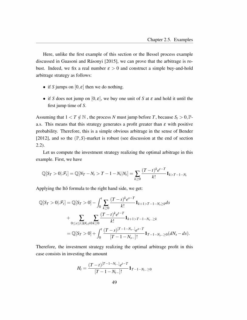
Chapter 2.5. Examples
Here, unlike the first example of this section or the Bessel process examplediscussed in Guasoni and Rasonyi [2015], we can prove that the arbitrage is ro-bust. Indeed, we fix a real number ε > 0 and construct a simple buy-and-holdarbitrage strategy as follows:
• if S jumps on [0,ε] then we do nothing.
• if S does not jump on [0,ε], we buy one unit of S at ε and hold it until thefirst jump time of S.
Assuming that 1 < T /∈ N , the process N must jump before T , because St > 0,P-a.s. This means that this strategy generates a profit greater than ε with positiveprobability. Therefore, this is a simple obvious arbitrage in the sense of Bender[2012], and so the (P,S)-market is robust (see discussion at the end of section2.2).
Let us compute the investment strategy realizing the optimal arbitrage in thisexample. First, we have
Q[ST > 0|Ft ] =Q[NT −Nt > T −1−Nt |Nt ] = ∑k≥0
(T − t)ket−T
k!1k>T−1−Nt
Applying the Ito formula to the right hand side, we get:
Q[ST > 0|Ft ] =Q[ST > 0]−∫ t
0∑k≥0
(T − s)kes−T
k!1k+1>T−1−Ns≥kds
+ ∑0≤s≤t:∆Ns 6=0
∑k≥0
(T − t)ket−T
k!1k+1>T−1−Ns−≥k
=Q[ST > 0]+∫ t
0
(T − s)[T−1−Ns−]es−T
[T −1−Ns−]!1T−1−Ns−≥0(dNs−ds).
Therefore, the investment strategy realizing the optimal arbitrage profit in thiscase consists in investing the amount
Ht =(T − t)[T−1−Nt−]et−T
[T −1−Nt−]!1T−1−Nt−≥0
49

Chapter 2.5. Examples
into the risky asset at every date t ∈ [0,T ]. This strategy is not buy-and-hold, butit is of finite variation, which means that a small perturbation of the price processwill correspond to a small modification of the arbitrage gain, showing that notonly the mere presence of the arbitrage is robust to frictions, but also the strategyrealizing the optimal arbitrage is robust.
The optimal wealth. In this example, the optimal wealth process can be com-puted explicitly. By Markov property, we have
EQ [1τ>T |Ft ] = Q [St +Ns−λ s > 0,0≤ s≤ T − t] := h(t,St) .
Next, we denote τx = inft > 0 : Nt ≤−x+λ t and the quantity h(t,x) becomesQ [τx > T − t]. We observe that τx is a discrete random variable with values in x
λ, x+1
λ, ...
and its distribution is given below,
Q[τx =
xλ
]= Q
[N x
λ= 0]= e−λ
xλ = e−x,
Q[
τx =x+1
λ
]= Q
[Nx+1
λ
= 1,N xλ= 1]
= Q[
Nx+1λ
−N xλ= 0∣∣∣N x
λ= 1]
Q[N x
λ= 1]
= Q[N 1
λ
= 0]
Q[N x
λ= 1]= e−λ
1λ e−λ
xλ λ
xλ= xe−x−1, ...
Remark 2.5.1. Arbitrage opportunities can be exploited by a differential-differenceequation. We consider the following function
h(t,x) = EQ [1x+NT−t−λ (T−t)≥0]=
∞
∑k=0
e−λ (T−t) (λ (T − t))k
k!1x+k−λ (T−t)≥0.
The function h is not continuous on the lines x+ k−λ (T − t) = 0. Outside theselines, h is differentiable. The equation for h is
∂h∂ t− ∂h
∂xλ +h(t,x+1)−h(t,x)λ = 0
h(T,x) = 1x≥0.
50
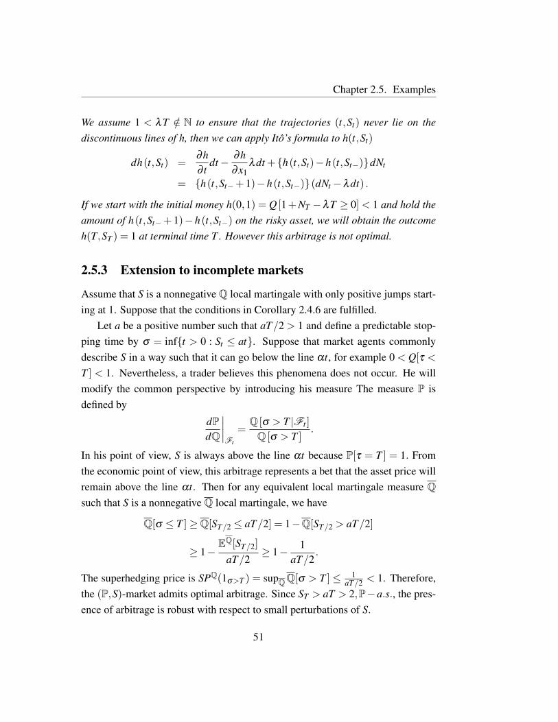
Chapter 2.5. Examples
We assume 1 < λT /∈ N to ensure that the trajectories (t,St) never lie on thediscontinuous lines of h, then we can apply Ito’s formula to h(t,St)
dh(t,St) =∂h∂ t
dt− ∂h∂x1
λdt +h(t,St)−h(t,St−)dNt
= h(t,St−+1)−h(t,St−)(dNt−λdt) .
If we start with the initial money h(0,1) = Q [1+NT −λT ≥ 0]< 1 and hold theamount of h(t,St−+1)−h(t,St−) on the risky asset, we will obtain the outcomeh(T,ST ) = 1 at terminal time T . However this arbitrage is not optimal.
2.5.3 Extension to incomplete markets
Assume that S is a nonnegative Q local martingale with only positive jumps start-ing at 1. Suppose that the conditions in Corollary 2.4.6 are fulfilled.
Let a be a positive number such that aT/2 > 1 and define a predictable stop-ping time by σ = inft > 0 : St ≤ at. Suppose that market agents commonlydescribe S in a way such that it can go below the line αt, for example 0 < Q[τ <
T ] < 1. Nevertheless, a trader believes this phenomena does not occur. He willmodify the common perspective by introducing his measure The measure P isdefined by
dPdQ
∣∣∣∣Ft
=Q [σ > T |Ft ]
Q [σ > T ].
In his point of view, S is always above the line αt because P[τ = T ] = 1. Fromthe economic point of view, this arbitrage represents a bet that the asset price willremain above the line αt. Then for any equivalent local martingale measure Qsuch that S is a nonnegative Q local martingale, we have
Q[σ ≤ T ]≥Q[ST/2 ≤ aT/2] = 1−Q[ST/2 > aT/2]
≥ 1−EQ[ST/2]
aT/2≥ 1− 1
aT/2.
The superhedging price is SPQ(1σ>T ) = supQQ[σ > T ] ≤ 1aT/2 < 1. Therefore,
the (P,S)-market admits optimal arbitrage. Since ST > aT > 2,P−a.s., the pres-ence of arbitrage is robust with respect to small perturbations of S.
51

Chapter 2.5. Examples
2.5.4 A variation: building an arbitrage from a bubble
Let S be a nonnegative Q local martingale with no positive jumps, satisfying S0 =1 and St ≤ ε < 1, Q-a.s for t ≥ T . Because the process S is a strict local martingaleunder Q (its expectation at time T is less than 1), the market admits a bubble.
We define σ = inft ≥ 0 : St > K for K > 1. In this example, a trader believesthat the price of S may not exceed an upper bound K. As in previous examples, thistrader may construct an arbitrage model P as in (2.6), provided that the conditionsin Corollary 2.4.6 are fulfilled. Under any ELMM Q, Sσ∧t is a bounded Q localmartingale and hence a Q martingale. So we get
1 = EQ[Sσ∧T ] = KQ[σ ≤ T ]+EQ[ST 1σ>T ],
and therefore
Q[σ ≤ T ] =1−EQ[ST 1σ>T ]
K>
1− ε
K.
The superhedging price of 1σ>T is
supQ∈ELMM(Q,S)
EQ[1σ>T ]< 1− 1− ε
K< 1.
2.5.5 A joint bet on an asset and its volatility
Let S and ξ be continuous Ito processes with dynamics,
dSt = ξtdWQt , S0 = 1,
dξt = a(t,ξt)ξtdt +b(t,ξt)ξtdWQt ,
where (WQ,WQ) is a standard two-dimensional Brownian motion and the coef-
ficients a and b are such that the equation for ξ admits a strong solution and inaddition
K−1 < b(t,x)< K and a(t,x)< K
for all t, all x > 0 and some constant K > 1. We assume that the filtration F =
(Ft)0≤t≤T is given by Ft = FWQt ∨FWQ
t .
52

Chapter 2.5. Examples
Let ξ < ξ0 and define stopping times as follows:
σ1 := inft > 0 : St ≤ 0, σ2 := inft > 0 : ξt ≤ ξ, σ = σ1∧σ2.
This choice of the stopping time represents a bet that S will not hit 0 and itsvolatility will stay above ξ up to time T .
Let us check the conditions in Corollary 2.4.6. Given that S and ξ are contin-uous, the only nontrivial part is to show that for every stopping time θ ∈ [0,T ],
Q[σ > T |Fθ ] =Q[σ1 > T ,σ2 > T |Fθ ]> 0 (2.16)
on σ > θ.By Theorem 3.2 in Pakkanen [2010], logξ has the FWQ
-conditional full sup-port property, which implies (by Lemma 2.1 in the above reference), that the prob-ability that logξ stays in a small ball around any continuous function between timet and time T , conditional on FWQ
t is strictly positive. This in turn means that
Q[σ2 > T |FWQ
θ ]> 0
on σ2 > θ. Since WQ is independent from ξ , by Theorem 3.1 in the above ref-erence, S has the conditional full support property also with respect to the filtrationFt ∨σ(ξs,0≤ s≤ T ), i.e.
Q[σ1 > T |Fθ ∨σ(ξs,0≤ s≤ T )]> 0
on σ > θ. Together with the full support property of logξ , this implies (2.16),i.e. on σ > θ
Q[σ1 > T,σ2 > T |Fθ ] = E [E[1σ1>T |Ft ∨σ(ξs,0≤ s≤ T )]1σ2>T |Fθ ]> 0.
Then, under any equivalent local martingale measure Q, we have
Q[σ ≤ T ] =Q[σ1 ≤ T,σ2 > T ]+Q[σ2 ≤ T ]
≥Q[ inf0≤u≤ξ
2TBu ≤−1,σ2 > T ]+Q[σ2 ≤ T ]≥Q[ inf
0≤u≤ξ2T
Bu ≤−1]> 0,
53
Chapter 2.5. Examples
where B is the Brownian motion such that
t∫0
ξudWQu = B∫ t
0 ξ 2u du
a.s. for all t ≥ 0. Thus, Q[σ ≤ T ] is bounded from below by the quantityQ[inf0≤u≤ξ
2T Bu ≤−1]. This quantity is positive and does not depend on Q, since
B is a Brownian motion under Q. Therefore supQQ[σ > T ] is bounded away fromone and the superhedging price satisfies SPQ(1σ>T ) = supQQ[σ > T ]< 1.
2.5.6 A variation: betting on the square bracket
The construction in Example 2.5.5 can be modified as follows. Let S be a contin-uous Q-local martingale with S0 = 1. We define
σ1 := inft > 0 : St ≤ 0, σ2 := inft > 0 : [S]t ≤−a+bt, σ = σ1∧σ2,
where a,b are positive constants. Suppose that the conditions in Corollary 2.4.6are fulfilled (they can be checked under suitable assumptions using the conditionalfull support property similarly to how this was done in the previous example).Then under any ELMM Q, we compute
Q[σ ≤ T ] =Q[σ1 ≤ T,σ2 > T ]+Q[σ2 ≤ T ]
=Q[ inf0≤u≤[S]T
Bu ≤−1,σ2 > T ]+Q[σ2 ≤ T ]≥Q[ inf0≤u≤bT−a
Bu ≤−1]> 0,
where B is the Brownian motion such that St = B[S]t a.s. for all t ≥ 0. Thus thesuperhedging price satisfies SPQ(1σ>T ) = supQQ[σ > T ]< 1.
54

Chapter 3
Optimal investment withintermediate consumption under nounbounded profit with bounded risk
Abstract: We consider the problem of optimal investment with intermediate con-sumption in a general semimartingale model of an incomplete market, with pref-erences being represented by a utility stochastic field. We show that the key con-clusions of the utility maximization theory hold under the assumptions of no un-bounded profit with bounded risk (NUPBR) and of the finiteness of both primaland dual value functions.
Key words: utility maximization, unbounded profit with bounded risk, arbi-trage of the first kind, local martingale deflator, duality theory, semimartingale,incomplete markets.
This chapter is based on joint work with Andrea Cosso, Claudio Fontana andOleksii Mostovyi.
55

Chapter 3.1. Introduction
3.1 Introduction
Since the pioneering work of Harrison and Kreps [1979], equivalent local/sigmamartingale measures play a prominent role in the problems of pricing and portfoliooptimization. Their existence is equivalent to the absence of arbitrage in the senseof no free lunch with vanishing risk (NFLVR) and this represents the crucial no-arbitrage-type assumption in the classical duality approach to optimal investmentproblems (see e.g. Karatzas and Zitkovic [2003]; Kramkov and Schachermayer[1999, 2003]; Zitkovic et al. [2005]). In a general semimartingale setting, nec-essary and sufficient conditions for the validity of the key assertions of the utilitymaximization theory (with the possibility of intermediate consumption) have beenrecently established in Mostovyi [2015]. More specifically, such assertions havebeen proven in Mostovyi [2015] under the assumptions that the primal and dualvalue functions are finite and that there exists an equivalent martingale deflator.In particular, in a finite time horizon, the latter assumption is equivalent to thevalidity of NFLVR.
In this chapter, we consider a general semimartingale setting in an infinite timehorizon where preferences are modeled via a utility stochastic field, allowing forintermediate consumption. Building on the abstract theorems of Mostovyi [2015],our main result shows that the standard assertions of the utility maximization the-ory hold true as long as there is no unbounded profit with bounded risk (NUPBR)and both primal and dual value functions are finite. In general, NUPBR is weakerthan NFLVR and can be shown to be equivalent to the existence of an equivalentlocal martingale deflator. Our results give an affirmative answer to a widespreadconjecture in the mathematical finance community stating that the key conclusionsof the utility maximization theory hold under NUPBR.
The proofs rely on certain characterizations of the dual feasible set. Thus, inLemma 3.3.2 we give a polarity description, show its closedness under countableconvex combinations in Lemma 3.3.3, and demonstrate in Proposition 3.2.1 thatnonemptyness of the set that generates the dual domain is equivalent to NUPBR.Upon that, we prove the bipolar relations between primal and dual feasible setsand apply the abstract theorems from Mostovyi [2015]. As an implication of
56

Chapter 3.1. Introduction
the bipolar relations, we also show how Theorem 2.2 in Kramkov and Schacher-mayer [1999] can be extended to hold under NUBPR (instead of NFLVR), seeRemark 3.2.5 below for details.
Neither NFLVR, nor NUPBR by itself guarantee the existence of solutions toutility maximization problems, see [Kramkov and Schachermayer, 1999, Exam-ple 5.2] and [Christensen and Larsen, 2007, Example 4.3] for counterexamples.This is why finiteness of the value functions is needed in the formulation of ourmain result. However, it is shown in Choulli et al. [2015] that NUPBR holds ifand only if, for every sufficiently nice deterministic utility function, the problemof maximizing expected utility from terminal wealth admits a solution under anequivalent probability measure, which can be chosen to be arbitrarily close to theoriginal measure (see [Choulli et al., 2015, Theorem 2.8] for details). Besides,no unbounded profit with bounded risk represents the minimal no-arbitrage-typeassumption that allows for the standard conclusions of the theory to hold for theutility maximization problem from terminal wealth. Indeed, by [Karatzas andKardaras, 2007, Proposition 4.19], the failure of NUPBR implies that there existsa time horizon such that the corresponding utility maximization problem eitherdoes not have a solution, or has infinitely many. Our work complements thesepapers by providing the convex duality results under NUPBR, also allowing forstochastic preferences as well as intermediate consumption.
The problem of utility maximization without relying on the existence of mar-tingale measures has already been addressed in the literature. In the very first pa-per Merton [1969] on expected utility maximization in continuous time settings,an optimal investment problem is explicitly solved even though an equivalent mar-tingale measure does not exist in general in the infinite time horizon case. In anincomplete Ito process setting under a finite time horizon, Karatzas et al. [1991]have considered the problem of maximization of expected utility from terminalwealth and established the existence results for an optimal portfolio via convexduality theory without the full strength of NFLVR (see also [Fernholz et al., 2009,Section 10.3] and [Fontana and Runggaldier, 2013, Section 4.6.3]). In particu-lar, in view of [Kardaras, 2010, Theorem 4], Assumption 2.3 in Karatzas et al.
57

Chapter 3.1. Introduction
[1991] is equivalent to the nonemptyness of the set of equivalent local martingaledeflators. Passing from an Ito process to a continuous semimartingale setting, theresults of Kramkov and Schachermayer [1999] have been extended by weakeningthe NFLVR requirement in Larsen [2009] (note that [Larsen, 2009, Assumption2.1] is equivalent to NUPBR). In a general semimartingale setting, Larsen andZitkovic [2013] have established convex duality results for the problem of max-imizing expected utility from terminal wealth (for a deterministic utility func-tion) in the presence of trading constraints without relying on the existence ofmartingale measures. In particular, in the absence of trading constraints, the no-arbitrage-type requirement adopted in Larsen and Zitkovic [2013] turns out tobe equivalent to NUPBR. Indeed, [Larsen and Zitkovic, 2013, Assumption 2.3]requires the L0
+-solid hull1 of the set of all terminal wealths generated by admis-sible strategies with initial wealth x, denoted by C (x), to be convexly compact2
for all x ∈ R and nonempty for some x ∈ R. In the absence of trading constraints,[Kardaras, 2010, Theorem 2] shows that the boundedness in L0 of C (x) alreadyimplies its closedness in L0, thus in such a framework the convex compactness ofC (x) holds if and only if the NUPBR condition does.
The chapter is structured as follows. Section 3.2 begins with a description ofthe general setting (Subsection 3.2.1), introduces and characterizes the NUPBRcondition (Subsection 3.2.2) and then proceeds with the statement of the mainresults (Subsection 3.2.3). Section 3.3 contains the proofs of our results.
1As usual, L0 denotes the space of equivalence classes of real-valued random variables on theprobability space (Ω,F ,P), equipped with the topology of convergence in probability; L0
+ is thepositive orthant of L0.
2See [Zitkovic, 2010, Definition 2.1] for the definition of convex compactness, a convenientcharacterization of which is given by [Zitkovic, 2010, Theorem 3.1]: “a closed and convex subsetof L0
+ is convexly compact if and only if it is bounded in probability”.
58
Chapter 3.2. Setting and main results
3.2 Setting and main results
3.2.1 Setting
Let (Ω,F ,(Ft)t∈[0,∞),P) be a complete stochastic basis, with F0 being the com-pletion of the trivial σ -algebra, and S = (St)t≥0 an Rd-valued semimartingale 3,representing the discounted prices of d risky assets. We fix a stochastic clockκ = (κt)t≥0 which is a nondecreasing, cadlag adapted process such that
κ0 = 0, P(κ∞ > 0)> 0 and κ∞ ≤ A, (3.1)
for some finite constant A. The stochastic clock κ represents the notion of timeaccording to which consumption occurs. By suitably specifying the clock processκ , several different formulations of investment problems, with or without interme-diate consumption, can be recovered from the present setting (compare e.g. with[Zitkovic et al., 2005, Section 2.8] and [Mostovyi, 2015, Examples 2.5-2.9]).
A portfolio is defined by a triplet Π = (x,H,c), where x ∈ R represents aninitial capital, H = (Ht)t≥0 is an Rd-valued predictable S-integrable process rep-resenting the holdings in the d risky assets and c = (ct)t≥0 is a nonnegative op-tional process representing the consumption rate. The discounted value processV = (Vt)t≥0 of a portfolio Π = (x,H,c) is defined as
Vt := x+∫ t
0Hu dSu−
∫ t
0cu dκu, t ≥ 0.
We let X be the collection of all nonnegative value processes associated to port-folios of the form Π = (1,H,0), i.e.,
X :=
X ≥ 0 : Xt = 1+∫ t
0Hu dSu, t ≥ 0
.
For a given initial capital x > 0, a consumption process c is said to be x-admissible(written as c ∈ Ax) if there exists an Rd-valued predictable S-integrable process
3It’s remarked that the assumptions of this present chapter is slightly different from the generalsetting introduced in Section 1.4.
59

Chapter 3.2. Setting and main results
H such that the value process V associated to the portfolio Π = (x,H,c) is non-negative. For brevity, we let A := A1. We remark that the set A in this presentchapter involves a property for consumption processes, not for strategies as in thegeneral setting in Section 1.4.
3.2.2 No unbounded profit with bounded risk
In this paper, we shall assume the validity of the following no-arbitrage-type con-dition:
the set X (T ) :=
XT : X ∈X
is bounded in probability, for all T ≥ 0.(NUPBR)
For each T ≥ 0, the boundedness in probability of the set X (T ) has been namedno unbounded profit with bounded risk in Karatzas and Kardaras [2007] and, asshown in Proposition 1 of Kardaras [2010], is equivalent to the absence of arbi-trages of the first kind on [0,T ]. Hence, condition NUPBR is equivalent to theabsence of arbitrages of the first kind in the sense of Definition 1 of Kardaras[2014].
We define the set of equivalent local martingale deflators (ELMD) as follows:
Z :=
Z > 0 : Z is a cadlag local martingale such that Z0 = 1 and
ZX is a local martingale for every X ∈X.
The following result is already known in the one-dimensional case in finitehorizon (see e.g. [Kardaras, 2012, Theorem 2.1]). Since we could not find aspecific reference for our formulation in the multi-dimensional case in infinitehorizon, we provide a detailed proof in Section 3.3. The condition (NUPBR) ininfinite horizon is also discussed in Definition 2.1 and Remark 2.2 of Aksamitet al. [2014].
Proposition 3.2.1. NUPBR holds if and only if Z 6= /0.
Remark 3.2.2. In Mostovyi [2015], it is assumed that the set
Z ∈Z : Z is a martingale 6= /0.
60

Chapter 3.2. Setting and main results
In view of Proposition 3.2.1, the latter condition is stronger than NUPBR. Aclassical example where NUPBR holds but Z ∈ Z : Z is a martingale = /0 isprovided by the three-dimensional Bessel process (see e.g. Delbaen and Schacher-mayer [1995a] and Example 4.6 of Karatzas and Kardaras [2007]).
3.2.3 Optimal investment with intermediate consumption
We now proceed to show that the key conclusions of the utility maximizationtheory can be established under condition (NUPBR). We assume that preferencesare represented by a utility stochastic field U =U(t,ω,x) : [0,∞)×Ω× [0,∞)→R∪−∞ satisfying the following assumption (see Assumption 2.1 of Mostovyi[2015]).
Assumption 3.2.3. For every (t,ω) ∈ [0,∞)×Ω, the function x 7→U(t,ω,x) isstrictly concave, strictly increasing, continuously differentiable on (0,∞) and sat-isfies the Inada conditions
limx↓0
U ′(t,ω,x) = +∞ and limx→+∞
U ′(t,ω,x) = 0,
with U ′ denoting the partial derivative of U with respect to its third argument.By continuity, at x = 0 we have that U(t,ω,0) = limx↓0U(t,ω,x) (note this valuemay be +∞). Finally, for every x≥ 0, the stochastic process U(·, ·,x) is optional.
To a utility stochastic field U satisfying Assumption 3.2.3, we associate theprimal value function, defined as
u(x) := supc∈Ax
E[∫
∞
0U(t,ω,ct)dκt
], x > 0, (3.2)
with the convention E[∫
∞
0 U(t,ω,ct)dκt ] :=−∞ if E[∫
∞
0 U−(t,ω,ct)dκt ] = +∞.In order to construct the dual value function, we define as follows the stochas-
tic field V conjugate to U :
V (t,ω,y) := supx>0
(U(t,ω,x)− xy
), (t,ω,y) ∈ [0,∞)×Ω× [0,∞).
61

Chapter 3.2. Setting and main results
We also introduce the following set of dual processes:
Y (y) := cl
Y : Y is cadlag adapted and
0≤ Y ≤ yZ (dκ⊗P)-a.e. for some Z ∈Z,
where the closure is taken in the topology of convergence in measure (dκ ⊗P)on the space of real-valued optional processes. We write Y := Y (1) for brevity.The value function of the dual optimization problem (dual value function) is thendefined as
v(y) := infY∈Y (y)
E[∫
∞
0V (t,ω,Yt)dκt
], y > 0, (3.3)
with the convention E[∫
∞
0 V (t,ω,Yt)dκt ] :=+∞ if E[∫
∞
0 V+(t,ω,Yt)dκt ] = +∞.We are now in a position to state the following theorem, which is the main
result of this chapter.
Theorem 3.2.4. Assume that conditions (3.1) and (NUPBR) hold true and let Ube a utility stochastic field satisfying Assumption 3.2.3. Suppose that
v(y)< ∞ for all y > 0 and u(x)>−∞ for all x > 0. (3.4)
Then the value function u and the dual value function v defined in (3.2) and (3.3),respectively, satisfy the following properties:
(i) u(x)<∞, for all x> 0, and v(y)>−∞, for all y> 0. Moreover, the functionsu and v are conjugate, i.e.,
v(y) = supx>0
(u(x)− xy
), y > 0,
u(x) = infy>0
(v(y)− yx
), x > 0;
(ii) the functions u and −v are continuously differentiable on (0,∞), strictlyconcave, strictly increasing and satisfy the Inada conditions
u′(0) := limx↓0
u′(x) = +∞, −v′(0) := limy↓0− v′(y) = +∞,
u′(∞) := limx→+∞
u′(x) = 0, −v′(∞) := limy→+∞
− v′(y) = 0.
62

Chapter 3.3. Proofs
Moreover, for every x > 0 and y > 0, the solutions c(x) to (3.2) and Y (y) to (3.3)exist and are unique and, if y = u′(x), we have the dual relations
Yt(y)(ω) =U ′(t,ω, ct(x)(ω)
), dκ⊗P-a.e.,
and
E[∫
∞
0ct(x)Yt(y)dκt
]= xy.
Finally, the dual value function v can be equivalently represented as
v(y) = infZ∈Z
E[∫
∞
0V (t,ω,yZt)dκt
], y > 0. (3.5)
Remark 3.2.5. A close look at the proof of Theorem 3.2.4 reveals that for κ cor-responding to utility maximization from terminal wealth, the sets A and Y satisfythe assumptions of Proposition 3.1 in Kramkov and Schachermayer [1999]. Thisimplies that for a deterministic utility U satisfying the Inada conditions and suchthat AE(U)< 1 (in the terminology of Kramkov and Schachermayer [1999]), un-der an additional assumption of finiteness of u(x) for some x > 0, the assertionsof Theorem 2.2 in Kramkov and Schachermayer [1999] hold under (NUPBR)(and possibly without NFLVR). This is a consequence of “abstract” Theorem 3.1in Kramkov and Schachermayer [1999].
3.3 Proofs
Proof of Proposition 3.2.1. Suppose that NUPBR holds. Then, for every n ∈ N,the set Xn is bounded in L0 and, by [Takaoka and Schweizer, 2014, Theorem 2.6],there exists a strictly positive cadlag local martingale Zn such that Zn
0 = 1 (sinceF0 is trivial) and the Rd-valued process ZnS is a sigma-martingale on [0,n]. As aconsequence of [Ansel and Stricker, 1994, Corollary 3.5] (see also [Choulli et al.,2015, Remark 2.4]), it holds that ZnX is a local martingale on [0,n], for everyX ∈X and n ∈ N. For all t ≥ 0, let then n(t) := minn ∈ N : n > t and definethe cadlag process Z = (Zt)t≥0 via
Zt :=n(t)
∏k=1
Zkk∧t
Zk(k−1)∧t
, t ≥ 0.
63

Chapter 3.3. Proofs
We now claim that Z ∈Z . Since X ≡ 1 ∈X and in view of [Jacod and Shiryaev,2002, Lemma I.1.35], it suffices to show that, for every X ∈X , the process ZXis a local martingale on [0,m], for each m ∈ N. Fix m ∈ N. Consider an arbitraryX ∈X and let τn
k k∈N be a localizing sequence for the local martingale ZnX on[0,n], for each n ∈ 1, . . . ,m. Let τ
jk τ j
k< j:= τ
jk Iτ j
k< j+∞Iτ jk= j (which is a
stopping time by [Jacod and Shiryaev, 2002, §I.1.15]), for j = 1, . . . ,m and k ∈N,and define the stopping times
T mk := min
τ
1k τ1
k <1, . . . ,τmk τm
k <m,m, k ∈ N.
Similarly as in [Fontana et al., 2015, proof of Theorem 4.10], it can be readilyverified that the stopped proces (ZX)T m
k is a martingale on [0,m], for all k ∈ N.Since limk→+∞P(T m
k = m) = 1, this shows that ZX is a local martingale on [0,m].By the arbitrariness of m, this proves the claim.
To prove the converse implication, note that, for any X ∈ X and Z ∈ Z ,the process ZX is a supermartingale and, hence, for every T ≥ 0, it holds thatE[ZT XT ] ≤ 1. This shows that the set ZT XT is bounded in L1 and, hence, inL0. Since the multiplication by the finite random variable ZT does not affect theboundedness in L0, this implies that XT is bounded in L0, for all T ≥ 0.
Let us now turn to the proof of Theorem 3.2.4. Together with the abstractresults established in [Mostovyi, 2015, Section 3], the key step is represented bythe following lemma, which generalizes [Mostovyi, 2015, Lemmata 4.2 and 4.3]by relaxing the no-arbitrage-type requirement into condition NUPBR.
As a preliminary, for a semimartingale S, let us denote by H (S) the set of alladmissible integrands, in the sense of [Delbaen and Schachermayer, 1994, Defi-nition 2.7], and define the following sets of equivalent probability measures:
Mσ (S) :=Q∼ P : S is a Q-sigma-martingale
,
Mloc(S) :=Q∼ P :
∫H dS is a Q-local martingale for every H ∈H (S)
,
Ms(S) :=Q∼ P :
∫H dS is a Q-supermartingale for every H ∈H (S)
.
64

Chapter 3.3. Proofs
Lemma 3.3.1. Let S be a semimartingale. Then it holds that
Mσ (S)⊆Mloc(S)⊆Ms(S).
Moreover, if Ms(S) 6= /0, then Mσ (S) 6= /0 and the set Mσ (S) is dense in Ms(S)with respect to the norm of L1(Ω,F ,P).
Proof. Since the class of sigma-martingales is stable with respect to stochastic in-tegration (see [Jacod and Shiryaev, 2002, Proposition III.6.42]), the first inclusionfollows from [Ansel and Stricker, 1994, Corollary 3.5]. The second inclusionfollows from the fact that any local martingale bounded from below is a super-martingale. Finally, the last assertion follows from [Delbaen and Schachermayer,1998, Proposition 4.7], by noting that, if Ms(S) 6= /0, then S satisfies NFLVR, sothat Mσ (S) 6= /0 by [Delbaen and Schachermayer, 1998, Theorem 1.1].
The following lemma provides a polarity characterization of attainable con-sumption streams.
Lemma 3.3.2. Let c be a nonnegative optional process and κ a stochastic clock.Under assumptions (3.1) and NUPBR, the following conditions are equivalent:
(i) c ∈A ;
(ii) supZ∈Z E[∫
∞
0 ctZt dκt ]≤ 1.
Proof. If c ∈ A , there exists an Rd-valued predictable S-integrable process Hsuch that
1+∫ t
0Hu dSu ≥
∫ t
0cu dκu ≥ 0, t ≥ 0.
We define Ct :=∫ t
0 cu dκu, for t ≥ 0, and observe that C is an increasing process.For an arbitrary Z ∈Z , the process (
∫ t0 Cu− dZu)t≥0 is a local martingale and we let
τnn∈N be a localizing sequence such that (∫
C− dZ)τn is a uniformly integrablemartingale, for all n ∈ N. Using the supermartingale property of Z(1+
∫H dS),
we obtain for every n ∈ N
1≥ E[
Zτn
(1+
∫τn
0Hu dSu
)]≥ E [ZτnCτn] = E
[∫τn
0Zu dCu +
∫τn
0Cu− dZu
],
65

Chapter 3.3. Proofs
where the last equality follows by integration by parts (see [Jacod and Shiryaev,2002, Proposition I.4.49]). Since τnn∈N is a localizing sequence for
∫C− dZ, it
holds that E[∫
τn0 Cu− dZu] = 0, for all n ∈ N. Hence:
1≥ E[∫
τn
0Zu dCu
], for all n ∈ N.
By the monotone convergence theorem, we get that 1 ≥ limn→∞E[∫
τn0 Zu dCu] =
E[∫
∞
0 Zu dCu]. Since Z ∈Z is arbitrary, this proves the implication (i)⇒(ii).Suppose now that supZ∈Z E[
∫∞
0 ctZt dκt ]≤ 1. Take an arbitrary Z ∈Z and letρnn∈N be a sequence of stopping times increasing P-a.s. to infinity such thatZρn is a uniformly integrable martingale, for all n ∈ N. By Lemma 3.3.1, it holdsthat Mσ (Sρn) 6= /0, for all n ∈ N. For n ∈ N, let Q ∈Mσ (Sρn) and denote byM = (Mt)t≥0 its density process (i.e., dQ|Ft = Mt dP|Ft , for all t ≥ 0). LettingZ′ := MρnZ(Zρn)−1, the same arguments of [Stricker and Yan, 1998, Lemma 2.3]imply that Z′ ∈ Z . For an arbitrary stopping time τ ∈ T (with T denoting theset of all finite stopping times), it then holds that
EQ[Cτ∧ρn] = E[Mτ∧ρnCτ∧ρn] = E[Z′τ∧ρnCτ∧ρn]≤ 1,
where the last inequality follows from the assumption that supZ∈Z E[∫
∞
0 ctZt dκt ]≤1 by the same arguments used in the first part of the proof together with an appli-cation of Fatou’s lemma. By the arbitrariness of Q∈Mσ (Sρn) and τ ∈T togetherwith the denseness of Mσ (Sρn) in Ms(Sρn) (see Lemma 3.3.1), it then follows that
supQ∈Ms(Sρn)
supτ∈T
EQ[Cτ∧ρn] = supQ∈Mσ (Sρn)
supτ∈T
EQ[Cτ∧ρn ]≤ 1.
[Follmer and Kramkov, 1997, Proposition 4.2] (together with Examples 2.2 and4.1 therein) then gives the existence of an adapted cadlag process V n such thatV n
t ≥Ct∧ρn , for all t ≥ 0, and admitting a decomposition of the form
V nt =V n
0 +∫ t
0Hn
u dSρnu −An
t , t ≥ 0,
where Hn is an Rd-valued predictable Sρn-integrable process, An is an adapted in-creasing process with An
0 = 0 and V n0 = supQ∈Ms(Sρn),τ∈T EQ[Cτ∧ρn ]≤ 1. There-
66

Chapter 3.3. Proofs
fore, for every n ∈ N, we obtain
1+∫ t
0Hn
u dSu ≥V n0 +
∫ t
0Hn
u dSu =V nt +An
t ≥V nt ≥Ct , 0≤ t ≤ ρn.
Let Hn := HnI[[0,ρn]], for all n ∈ N. By [Follmer and Kramkov, 1997, Lemma5.2], we can construct a sequence of processes Y nn∈N, with Y n ∈ conv(1 +
Hn · S,1+ Hn+1 · S, . . .), n ∈ N, and a cadlag process Y such that ZY nn∈N isFatou-convergent 4 to a supermartingale ZY , for every strictly positive cadlag localmartingale Z such that ZX is a supermartingale for every X ∈X . Note that Yt ≥Ct , for all t ≥ 0, and Y0 ≤ 1. Similarly as above, applying then [Follmer andKramkov, 1997, Theorem 4.1] to the stopped process Y ρn , for n ∈ N, we obtainthe decomposition
Y ρnt = Y0 +
∫ t
0Gn
u dSρnu −Bn
t , t ≥ 0,
where Gn is an Rd-valued predictable Sρn-integrable process and Bn is an adaptedincreasing process with Bn = 0, for n ∈ N. Without loss of generality, we canassume that GnI]]ρn,+∞[[ = 0, for all n ∈ N. Letting G := G1 + ∑
∞n=1(G
n+1 −Gn)I]]ρn,+∞[[ = G1 +∑
∞n=1 Gn+1I]]ρn,ρn+1]], it follows that 1+
∫ t0 Gu dSu ≥Ct , for all
t ≥ 0, thus establishing the implication (ii)⇒(i).
We are now in a position to complete the proof of Theorem 3.2.4, which gen-eralizes the results of [Mostovyi, 2015, Theorems 2.3 and 2.4] to the case whereonly (NUPBR) is assumed to hold. As a preliminary, we need the following resulton the set Z .
Lemma 3.3.3. Under (NUPBR), the set Z is closed under countable convexcombinations. If in addition (3.1) holds, then for every c ∈A , we have
supZ∈Z
E[∫
∞
0ctZt dκt
]= sup
Y∈YE[∫
∞
0ctYt dκt
]≤ 1. (3.6)
4See [Follmer and Kramkov, 1997, Definition 5.2] for the definition of Fatou convergence ofstochastic processes.
67

Chapter 3.3. Proofs
Proof. Let Znn∈N be a sequence of processes belonging to Z and λ nn∈N asequence of positive numbers such that ∑
∞n=1 λ n = 1. Letting Z := ∑
∞n=1 λ nZn, we
need to show that Z ∈ Z . For each N ∈ N, define ZN := ∑Nn=1 λ nZn. For every
X ∈X , ZNXN∈N is an increasing sequence of nonnegative local martingales(i.e. ZN+1
t Xt ≥ ZNt Xt , for all N ∈N and t ≥ 0), such that ZN
t Xt converges a.s. to ZtXt
as N→ +∞, for every t ≥ 0, and Z0X0 = 1. The local martingale property of ZXthen follows from [Klein et al., 2014, Proposition 5.1] (note that its proof carriesover without modifications to the infinite horizon case), whereas [Dellacherie andMeyer, 1982, Theorem VI.18] implies that ZX is a cadlag process. Since X ∈X
is arbitrary and X ≡ 1 ∈X , this proves the claim.Finally, relation (3.6) follows by the same arguments used in [Mostovyi, 2015,
Lemma 4.3].
We denote by L0(dκ ×P) be the linear space of equivalence classes of real-valued optional processes on the stochastic basis (Ω,F ,(Ft)t∈[0,∞),P), equippedwith the topology of convergence in measure (dκ ×P). Let L0
+(dκ ×P) be thepositive orthant of L0(dκ×P).
Proof of Theorem 3.2.4. It is clear that the sets A and Y are convex solid subsetsof L0
+(dκ × P). By definition, Y is closed in the topology of convergence inmeasure (dκ ×P). As in [Mostovyi, 2015, part (i) of Proposition 4.4], a simpleapplication of Fatou’s lemma together with Lemma 3.3.2 allows to show that A
is also closed in the same topology. Moreover, by the same arguments used in[Mostovyi, 2015, part (ii) of Proposition 4.4], Lemma 3.3.2 together with thebipolar theorem of Brannath and Schachermayer [1999] implies that A and Y
satisfy the bipolar relations
c ∈A ⇐⇒ E[∫
∞
0ctYt dκt
]≤ 1 for all Y ∈ Y , (3.7)
Y ∈ Y ⇐⇒ E[∫
∞
0ctYt dκt
]≤ 1 for all c ∈A . (3.8)
Since X ≡ 1 ∈X and Z 6= /0, both A and Y contain at least one strictly positiveelement. In view of Lemma 3.3.3, Theorem 3.2.4 then follows directly from theabstract results of [Mostovyi, 2015, Theorems 3.2 and 3.3].
68

Chapter 3.3. Proofs
Acknowledgement
Oleksii Mostovyi’s work is supported by the National Science Foundation un-der award number DMS-1600307. Huy N. Chau’s work is supported by NatixisFoundation for Quantitative Research.
69

Chapter 3.3. Proofs
70

Chapter 4
Optimal arbitrage for initialfiltration enlargement
Abstract: This chapter studies optimal trading for an insider who has someadditional information at the beginning of the trading. Using the technique ofnon-equivalent measure change, we are able to provide a new criterion ensuringthat the market for the insider satisfies the condition No Unbounded Profit withBounded Risk (NUPBR), which excludes ’scalable’ arbitrages. Furthermore, ifthe condition NUPBR holds, we present a systematic way to exploit optimal arbi-trage opportunities.
Key words: No Unbounded Profits with Bounded Risk, optimal arbitrage,initial enlargement of filtration, incomplete markets, hedging.
This chapter is based on joint work with Peter Tankov and Wolfgang Rung-galdier.
Acknowledgement
Huy N. Chau’s work is supported by Natixis Foundation for Quantitative Re-search.
71

Chapter 4.1. Introduction
4.1 Introduction
In financial mathematics, theory of filtration enlargement is often used to modelinsider trading activities. This theory was developed in the seminal works of Ito,Barlow, Jacod, Jeulin and Yor and we refer to the book of Mansuy and Yor [2006]for an overview. By definition, an insider is a person who can access the privateinformation that others cannot. Consequently, the insider quickly incorporatessuch information to her trading strategies. One of the first papers on this topicis Pikovsky and Karatzas [1996], where the authors study the logarithmic utilityoptimization problem for the insider, who is able to anticipate the future, i.e. theterminal values of asset’s prices in Brownian settings. Whenever the logarithmicutility maximization problem for the insider is finite, the authors are able to com-pute it explicitly and give the optimal portfolio in closed form. Grorud and Pontier[1998] also compute logarithmic utility of the insider with consumption and pro-pose a statistical test whether or not a trader is an insider. Amendinger et al. [1998]relate the insider’s additional expected logarithmic utility with a relative entropy.This relation is then extended in Ankirchner et al. [2006]. For further references,we refer to Elliott and Jeanblanc [1999], Amendinger et al. [2003b], Hillairet[2005], Ankirchner et al. [2006], Ankirchner and Zwierz [2011], Danilova et al.[2010]... and others.
Apart from portfolio optimization, the question of arbitrage has also receivedconsiderable attention. Amendinger [2000] studies martingale representation prop-erties in the larger filtration. Imkeller et al. [2001] and Imkeller [2003] make useof Malliavin’s calculus in order to find semimartingale decompositions for someclasses of additional information which do not satisfy Jacod’s condition. In ad-dition, they prove that arbitrage opportunities exist in dramatic manners, in thesense that the so-called information drift has possibility of explosion. However,we will see later that the exploding information drift violates NUPBR (no un-bounded profit with bounded risk) condition. Recently, Acciaio et al. [2014] in-vestigated the stability of NUPBR for the insider with infinite horizon settings.They give a sufficient condition for the stability of NUPBR under initial filtrationenlargement. Basically, it is shown that if the risky asset and the density process
72

Chapter 4.1. Introduction
in Jacod’s condition do not jump at the same time, then the enlarged market sat-isfies NUPBR. However, Jacod’s condition is required at all times in their results,which cannot be always satisfied in finite horizon settings.
In this chapter, we focus on incomplete markets and examine the logarithmicutility maximization problems by using duality approach, rather than using theinformation drift or relative entropy as in all previous studies. By the techniqueof non-equivalent measure change as in Chapter 2, we are able to give a new dualrepresentation for the insider’s expected log-utility in quite general market mod-els. This duality result differs from classical results (see for example, Kramkovand Schachermayer [1999]) as it contains an extra term involving the entropy ofthe information. It is usually observed that the extra factor is the main reasonsuch that the insider’s expected utility blows up at the time when the private infor-mation becomes public. This new finding allows us to introduce a new criterionfor checking the condition NUPBR in the enlarged market with finite horizon set-tings. To do this, we first show that NUPBR always fails if the set of all martingaledensities for regular agents is uniformly integrable and an explicit construction ofunbounded profits is also given. Hence, the non-uniform integrability property is anecessary condition for the finiteness of the insider’s expected log-utility. It helpsto compensate explosive profits coming from the additional information, which inturn ensures NUPBR.
In the case NUPBR holds but not NFLVR, we present a new systematic ap-proach to find optimal arbitrage for the insider. We first study the case with dis-crete information, i.e. when the private information is given by a discrete randomvariable. The case with continuous random variable is treated by an approximat-ing procedure. Some illustrative examples are given.
The chapter is organized as follows. In Section 4.2, we provide some prelim-inaries on initial enlargement of filtrations. Section 4.3 introduces the notion ofsuperhedging and optimal arbitrage. Section 4.4 computes log-utility and optimalarbitrage when the information is given by a discrete random variable. Finally,the same questions for the case with continuous random variables are discussed inSection 4.5.
73

Chapter 4.2. Preliminaries on initial enlargement of filtrations
4.2 Preliminaries on initial enlargement of filtrations
Assume that the filtration F models the public information based on which ordi-nary agents make their decisions. We also suppose that the ordinary agents arerisk neutral, i.e. the (F,P)-market satisfies the condition NFLVR. The filtrationF is not necessarily the natural filtration of the stock prices. Suppose that thereis an insider who possesses from the beginning an additional information aboutthe value of some FT -measurable R-valued random variable G. In mathematicalterms, we model her knowledge by the enlarged filtration G= (Gt)t∈[0,T ] where
Gt :=⋂ε>0
(Ft+ε ∨σ(G)).
Note that we assume both that G is FT -measurable and that trading is possibleup to the terminal time T . This situation is known to be “difficult” (see e.g., theintroduction of Grorud and Pontier [1998]) and often leads to arbitrages of thefirst kind Amendinger et al. [1998]; our aim is to explore this setting in detail andidentify the cases where the NUPBR holds and optimal arbitrage strategies maybe found.
Because the semimartingale property is widely accepted in financial modeling,we first recall a condition of Jacod [1985] which ensures that a F-local martingaleremains a G-semimartingale. For all t ∈ [0,T ), let νt : Ω×R→ [0,1] be a regularversion of the Ft -conditional law of G and ν be the law of G. The followingassumption plays an important role in most studies in this theory.
Assumption 4.2.1. (Jacod’s Condition) For all t ∈ [0,T ), the regular conditionaldistribution of G given Ft is absolutely continuous with respect to the law of G,i.e. we have
νt ν , P−a.s. (4.1)
In particular, this assumption implies that G /∈Ft for all t < T . We emphasizethat this is a “weak” version of Jacod’s condition in the following sense.
• The absolute continuity of the measure νt with respect to the law of G isimposed only before the terminal time T . Of course, in our setting when
74

Chapter 4.2. Preliminaries on initial enlargement of filtrations
G ∈FT the absolute continuity cannot hold at the terminal date. When G /∈FT and νT ν , the NUPBR property can often be shown by constructinga local martingale deflator from the density process of νt with respect to ν ;in our setting this method is not avaiable.
• Only absolute continuity is imposed, rather than equivalence. If νt ∼ ν forall t ∈ [0,T ], then the density of νt with respect to ν is strictly positiveand one can show that NFLVR property holds by constructing an equiva-lent martingale measure from the density process. See Grorud and Pontier[1998], Theorem 3.2 of Amendinger [2000] or Follmer and Imkeller [1993]for details and related results. The situation when νt ∼ ν for t ∈ [0,T ) andνT ν is not fundamentally different from the situation when only absolutecontinuity is imposed on [0,T ].
The density of νt with respect to ν in Assumption 4.2.1 plays an importantrole in enlargement of filtration theory. Let O(F) be the F-optional sigma field onΩ×R+. It is shown in Lemme 1.8 and Corollaire 1.11 of Jacod [1985] that wecan even choose a nice version of the densities extracted from (4.1).
Lemma 4.2.2. Under Assumption 4.2.1, there exists a nonnegative B⊗O(F)-measurable function R×Ω×R+ 3 (x,ω, t) 7→ px
t (ω) ∈ [0,∞), cadlag in t suchthat
1. for every t ∈ [0,T ), we have νt(dx) = pxt (ω)ν(dx).
2. for each x ∈ R, the process (pxt (ω))t∈[0,T ) is a (F,P)-martingale.
3. The processes px, px− are strictly positive on [0,τx) and px = 0 on [τx,T ),
where
τx := inft ≥ 0 : px
t− = 0 or pxt = 0∧T.
Furthermore, if we define τG(ω) := τG(ω)(ω) then P[τG = T ] = 1.
The conditional density process pG is the key to find the semimartingale de-composition of a F-local martingale in the enlarged filtration G.
75

Chapter 4.2. Preliminaries on initial enlargement of filtrations
Proposition 4.2.3. Under Assumption 4.2.1, every F-local martingale X is a G-semimartingale on [0,T ) with decomposition
Xt = XGt +
t∫0
d⟨X , pG
.
⟩Fs
pGs−
(4.2)
where XG is a G-local martingale.
Passing a F-local martingale to the filtration G introduces a drift, i.e. a finitevariation term, in its semimartingale decomposition. This extra term measures thedifference of the information in the two filtrations.
Definition 4.2.4 (Information drift, Ankirchner et al. [2006]). Assume that S hasF-semimartingale decomposition S = M+α · 〈M,M〉. The G-predictable processµ satisfying
M−µ · 〈M,M〉 is a G-local martingale
is called information drift of M in the filtration G with respect to the filtration F.
In order to better understand the insider’s activities, we also need to study herstrategies. The structure of G-optional and G-predictable processes is given inProposition 2.3.1 of Jeanblanc [2010], reproduced below (this result was estab-lished in Jeulin [1980b] for discrete random variables and in Jeulin [1980a] forprogressive enlargement with a stopping time).
Proposition 4.2.5. Every G-optional process Y is of the form Yt(ω)= yt(ω,G(ω))
for some F⊗B(R)-optional process yt(ω,u).Every G-predictable process Y is of the form Yt(ω) = yt(ω,G(ω)) where
(t,ω,u) 7→ yt(ω,u) is a P(F)⊗B(R)-measurable function.
Finally, we make the following technical assumption.
Assumption 4.2.6. For every x, the process px does not jump to zero, i.e.
P[τx < T, pxτx− > 0] = 0.
76

Chapter 4.3. Optimal arbitrage
This assumption is introduced in Kardaras et al. [2015] for a general construc-tion of strict local martingales, in Ruf and Runggaldier [2013] for a constructionof markets with arbitrages and in Chapter 2 for the study of optimal arbitrage. Ac-ciaio et al. [2014] also use this assumption to prove the preservation of NUPBRunder the enlarged market. Basically, it requires that the conditional density px
goes to zero continuously. The meaning of this assumption can be interpreted asfollows. Let us consider an event G ∈ dx for some x ∈ R. This information isgiven for the insider at time zero, but not for regular agents, who can observe itat time T . However, regular agents can estimate the possibility of its occurrence,given their information. Hence, their perception is formulated by the density pro-cess px
t = P[G ∈ dx|Ft ]/P[G ∈ dx]. If the process px jumps to zero at time τx,it means that strictly before time τx, regular agents think that the event G ∈ dxis possible but at time τx, they suddenly realize that they are totally wrong. Inthe view of the insider, the event G ∈ dx is overestimated by regular agents andhence, the insider could make a profit by trading against them. Conversely, if thedensity px goes to zero continuously, regular agents realize that the probability ofthe event G ∈ dx gets smaller and smaller. The insider may gain some profitby trading against regular agents, however, the insider’s profit is not big (whichimplies no unbounded profit) because regular agents have time to correct theirbeliefs.
4.3 Optimal arbitrage
In Chapter 2, it is shown that optimal arbitrage is the inverse of the superhedgingprice of the claim 1. However, in the present chapter, we will emphasize that thereis a little difference in these concepts. First, we slightly adapt the definition ofsuperhedging price.
Definition 4.3.1. Let H∈F,G and let f ≥ 0 be a given claim. A H0-measurablerandom variable x∗( f ) is called the superhedging price of f with respect to H if
77

Chapter 4.4. Initial enlargement with a discrete random variable
there exists a H-predictable strategy H such that
x∗( f )+(H ·S)t ≥ 0, P−a.s,∀t ∈ [0,T ], (4.3)
x∗( f )+(H ·S)T ≥ f , P−a.s. (4.4)
and for each x ∈H0 which satisfies
x+(H ·S)t ≥ 0, P−a.s,∀t ∈ [0,T ],
x+(H ·S)T ≥ f , P−a.s,
one has x∗( f )≤ x,P−a.s.
In other words, the superhedging price of f is the minimal amount startingfrom which one can superhedge f by a nonnegative wealth process. However, theprice can be a true random variable if H0 is nontrivial. The definition of optimalarbitrage is given as follows, in conjunction with Lemma 2.3.3 of Chapter 2.
Definition 4.3.2 (Optimal arbitrage). We say that there is optimal arbitrage inthe market if x∗(1) ≤ 1 and P[x∗(1) < 1] > 0. If x∗(1) < 1,P− a.s., the optimalarbitrage is strong.
The condition NUPBR implies that x∗(1) is strictly positive, see Remark 2.3.4.The converse implication is not true. Indeed, we can find a market which satisfiesNA but not NUPBR, see Section 4 of Levental and Skorohod [1995]. Becausethe condition NA implies that x∗(1) > 0, the fact x∗(1) > 0 does not imply thatNUPBR holds.
4.4 Initial enlargement with a discrete random vari-able
Let us assume that G is a discrete random variable taking a finite number of valuesg1, ...,gn with nonzero probability. This is a “classical” case of initial filtrationenlargement, studied, e.g., in Aksamit [2014]; Jeulin [1980a,b]; Meyer [1978].
78

Chapter 4.4. Initial enlargement with a discrete random variable
In particular, it is known that every F-local martingale is a G-semimartingale on[0,T ] with decomposition
Xt = XGt +
n
∑i=1
1G=gi
∫ t
0
d〈X , pgi〉Fspgi
s−,
where XG is a G-local martingale. Therefore, it is not necessary to impose Ja-cod’s condition in this section. However, the additional assumption 4.2.6 will beimposed unless stated otherwise.
When the insider is informed that G will take the value gi where i ∈ 1, ...,n,she recognizes that all scenarios for the market’s evolution are contained in theevent G = gi. Consequently, she has no reason to keep using the original belief(probability measure P) in order to determine her investment strategy. The insiderwould like to update her belief by doing a measure change, i.e by dismissing allscenarios contained in G = g j for all j 6= i. To make this more concrete, weconsider the following measure transformation
dQi
dP
∣∣∣∣Ft
=P[G = gi|Ft ]
P[G = gi]:= pgi
t , i = 1, ...n. (4.5)
The measure Qi gives total mass to the event G = gi and is absolutely con-tinuous with respect to P but not equivalent to it. We shall use the techniquesdeveloped in Chapter 2 in this initial enlargement setting. In Section 4.4.1, wecompute the expected log-utility of the insider and then study under which cir-cumstances, the market for the insider satisfies the condition NUPBR. Next, wefind superhedging prices for the insider in Section 4.4.2. In Section 4.4.3 we givean example with a complete market where all computations are carried out. Sec-tion 4.4.4 gives an incomplete market example.
4.4.1 NUPBR and log-utility maximization
In this section, we will compute the insider’s expected log-utility. First, we relatethe expected utility of the insider to the expected utility of regular agents whenrestricted to an event G = gi.
79
Chapter 4.4. Initial enlargement with a discrete random variable
Lemma 4.4.1. The expected logarithmic utility for the insider can be representedas follows
supH∈A G
1
EP[logV 1,HT ] =
n
∑i=1
supH∈A F
1
EP[logV 1,HT 1G=gi]. (4.6)
Proof. The proof is easy and only requires representation of G-predictable pro-cesses as in Proposition 4.2.5. We do not use Assumption 4.2.6 here.(≤) Let HG ∈A G be a G-predictable strategy. By Proposition 4.2.5, the processHG is of the form HG
t (ω) = ht(ω,G(ω)) where ht(ω,x) is a P(F)×B(R)-measurable function. Then, HF,i = h(ω,gi) is F-predictable and HG1G=gi =
HF,i1G=gi a.s. Hence, we have that HG = ∑ni=1 HF,i1G=gi and therefore
∫ T
0HG
t dSt =n
∑i=1
1G=gi
∫ T
0HF,i
t dSt ,
where the equality follows from the fact that S is a G-semimartingale.We then compute
EP[logV 1,HG
T ] =n
∑i=1
EP[1G=gi logV 1,HF,i
T
].
Taking the supremum over the set of all G-admissible strategies we obtain theinequality (≤) in (4.6).(≥) For all HF,i, the following inequality holds true
n
∑i=1
EP[1G=gi logV 1,HF,i
T
]= EP[logV 1,HG
T ]≤ supH∈A G
1
EP[logV 1,HT ].
So, the proof is complete.
The usefulness of this lemma is that it transforms the insider’s maximizationproblem to many problems of regular agents under measure changes as in (4.5),up to a constant. As in the framework of NFLVR, it would be interesting to relatethe problem of maximizing log-utility under Qi to the problem of minimizing anappropriate function of deflators by duality. However, the equivalence between P
80
Chapter 4.4. Initial enlargement with a discrete random variable
and Qi is not preserved and it is no longer true that the condition NFLVR holdsunder Qi. The classical results, see for example Kramkov and Schachermayer[1999, 2003], cannot be applied here. This is not really bad news because as soonas Assumption 4.2.6 is valid, it can be proved that the (F,Qi)-market satisfiesthe condition NUPBR and the duality approach is still applicable, see Chapter 3.Nevertheless, coming back to the original measure P introduces an extra term, asseen in the next lemma.
Lemma 4.4.2. Under Assumption 4.2.6,
supH∈A F
1
EP[1G=gi logV 1,HT ] =−P[G = gi] logP[G = gi]
+ infZ∈ELMM(F,P)
EP[
1G=gi log1
ZT
], i ∈ 1, ...n.
Proof. For each i ∈ 1, ...,n, the (F,Qi)-market is obtained from the (F,P)-market by an absolutely continuous measure change, see Equation (4.5). Fur-thermore, the density process pgi does not jump to zero, by Assumption 4.2.6.Theorem 2.4.1 in Chapter 2 shows that the (F,Qi)-market satisfies the conditionNUPBR and for any local martingale density Z ∈ ELMM(F,P), the process Z/pgi
is a local martingale deflator for the (F,Qi)-market (note that on G= gi, pgit > 0
for all t). Let us introduce the following subsets of L0+
C (x) := v ∈ L0+ : 0≤ v≤ xV 1,HF
T , for some HF ∈A1,D(y) :=
z ∈ L0
+ : 0≤ z≤ yZT , for some Z ∈ ELMM(F,P),
D i(y) :=
zi =z
pgiT,z ∈D(y)
.
Because the (F,P)-market satisfies NFLVR, Proposition 3.1 of Kramkov and Schacher-mayer [1999] implies that C and D are convex with the following properties
v ∈ C (1) ⇐⇒ EP[vz]≤ 1, for all z ∈D(1),
z ∈D(1) ⇐⇒ EP[vz]≤ 1, for all v ∈ C (1).
81

Chapter 4.4. Initial enlargement with a discrete random variable
These imply that
v ∈ C (1) ⇐⇒ EQi[vzi]≤ 1, for all zi ∈D i(1),
zi ∈D i(1) ⇐⇒ EQi[vzi]≤ 1, for all v ∈ C (1)
and thus the condition (3.1) of Mostovyi [2015] holds under the measure Qi. Inaddition, C and D i contain at least one strictly positive element. For all y > 0, thefiniteness of the dual optimization
infzi∈D i(y)
EQi[
log1zi
]is deduced from infZ∈ELMM(F,P)EP[log(1/ZT )] < ∞. Furthermore, for all x >
0, we have that supv∈C (x)EQi[logv] > −∞. An application of Theorem 3.2 of
Mostovyi [2015] shows that
supH∈A F
1
EQi[logV 1,H
T ] = infZ∈ELMM(F,P)
EQi[
logpgi
TZT
]and both sides of the equality are attainable. Hence,
supH∈A F
1
EP[1G=gi logV 1,HT ] = inf
Z∈ELMM(F,P)EP[
1G=gi logpgi
TZT
]= inf
Z∈ELMM(F,P)EP[
1G=gi log pgiT +1G=gi log
1ZT
]=−P[G = gi] logP[G = gi]+ inf
Z∈ELMM(F,P)EP[
1G=gi log1
ZT
].
The proof is complete.
Remark 4.4.3. Because the (F,Qi)-market satisfies the condition NUPBR, onecan use the results in Chapter 3 for the log-utility optimization problem under(F,Qi), i.e. the set of local martingale deflators of the (F,Qi)-market will beconcerned. However, we would like to represent the insider’s value function interms of ordinary agents’ martingale densities. So we use the abstract results ofMostovyi [2015].
82

Chapter 4.4. Initial enlargement with a discrete random variable
Lemma 4.4.1 and Lemma 4.4.2 lead to a new characterization of the expectedlog-utility of the insider in terms of the additional information G and the set of alllocal martingale densities of the (F,P)-market.
Theorem 4.4.4. Under Assumption (4.2.6),
supH∈A G
1
EP[logV 1,HT ] =−
n
∑i=1
P[G = gi] logP[G = gi],
+n
∑i=1
infZ∈ELMM(F,P)
EP[
1G=gi log1
ZT
]. (4.7)
It is remarked that whenever each optimization problem under Qi is attainablethen the optimization for the insider is also attainable. This theorem is useful forseveral reasons. First, it shows how to compute the insider’s profit. Let us con-sider the two components in the RHS of (4.7). The first component, which is theentropy of G, always contributes to the profit of the insider and does not dependon the structure of the (F,P)-market. The second component can be interpretedas the value of G with respect to the (F,P)-market. The expected log-utility forthe insider is finite if each component is finite, or if the second component com-pensates the first component. As a result, this theorem provides a tool to checkNUPBR under G.
Let us compare our results with the results in Amendinger et al. [1998]. Theadditional expected log-utility of the insider is denoted by
∆(F,G) := supH∈A G
1
EP[logV 1,HT ]− sup
H∈A F1
EP[logV 1,HT ].
In their approach, the quantity ∆(F,G) is represented by the information drift, seeDefinition 3.6 in their paper, and in our approach, it can be expressed as
−n
∑i=1
P[G = gi] logP[G = gi]+n
∑i=1
infZ∈ELMM(F,P)
EP[
1G=gi log1
ZT
]− inf
Z∈ELMM(F,P)EP[
log1
ZT
]. (4.8)
83
Chapter 4.4. Initial enlargement with a discrete random variable
If the market is complete, the two approaches end up with the same result: thequantity in (4.8) reduces to the entropy of G, which is exactly what is stated inTheorem 4.1 of Amendinger et al. [1998].
4.4.2 Superhedging and optimal arbitrage
In this section, we turn to the problem of superhedging for the insider. Under G,we note that the initial capital is a G0-measurable random variable, which meansthat we do not start with the same capital for all scenarios since G0 is not a trivialsigma algebra. However, it is not surprising that the capital is constant on eachevent G = gi.
Theorem 4.4.5. Under Assumption 4.2.6, the (G,P)-market satisfies NUPBR andthe superhedging price of a claim f in this market is given by
xG,P∗ ( f ) =
n
∑i=1
xF,P∗ ( f 1G=gi)1G=gi,
and the associated hedging strategy is HF,i1G=gi, where HF,i is the suphedgingstrategy for f 1G=gi in the (F,P)-market, i.e.
xF,P∗ ( f 1G=gi)1G=gi+(HF,i1G=gi ·S)T ≥ f 1G=gi,P−a.s.
Proof. The first statement is proved by contradiction, noticing that NUPBR isequivalent to NA1. Assume that there is an arbitrage of the first kind in the (G,P)-market, i.e. we can find a FT -random variable ξ (because FT = GT ) such thatP[ξ ≥ 0] = 1,P[ξ > 0]> 0 and for all ε > 0, there exists a G-predictable strategyHG,ε which satisfies
ε +(HG,ε ·S)T ≥ ξ ,P−a.s. (4.9)
Choose an index i such that P[ξ > 0∩G = gi]> 0. The inequality (4.9) stillholds true under Qi
ε +(HG,ε1G=gi ·S)T ≥ ξ ,Qi−a.s. (4.10)
84

Chapter 4.4. Initial enlargement with a discrete random variable
Let us look at the hedging strategy HG,ε1G=gi under Qi. Using the argumentas in the proof of Lemma 4.4.1, we have that HG,ε1G=gi = HF,i,ε1G=gi, whereHF,i,ε is a F-predictable strategy. Thus, (4.10) implies that ξ is an arbitrage ofthe first kind in the (F,Qi)-market, which is equivalent to the failure of NUPBR.However, by Theorem 2.4.1 of Chapter 2, the condition NUPBR holds for the(F,Qi)-market, see the argument in the proof of Lemma 4.4.2. This contradictionmeans that the first statement is proved.
For the second statement, we compute the superhedging prices of f under thenew measures Qi, i = 1..,n, again by using Theorem 2.4.1 of Chapter 2
xF,Qi
∗ ( f ) = xF,P∗ ( f 1G=gi).
For each i, we denote by HF,i the F- strategy which superhedges f under the(F,Qi)-market, that is
xF,Qi
∗ ( f )+(HF,i ·S)T ≥ f ,Qi−a.s.
This inequality holds also under P when restricted on G = gi
xF,P∗ ( f 1G=gi)1G=gi+(HF,i1G=gi ·S)T ≥ f 1G=gi,P−a.s.
Summing up these inequalities we obtain(∑
ixF,P∗ ( f 1G=gi)1G=gi
)+
(∑
iHF,i1G=gi
)·ST ≥ f ,P−a.s.
The hedging strategy(∑i HF,i1G=gi
)is G-predictable.
Finally, we prove that the initial capital ∑i xF,P∗ ( f 1G=gi)1G=gi is exactly thesuperhedging price of f in the (G,P)-market. Assume that y is a G0-measurablerandom variable such that
y+(HG ·S)T ≥ f ,P−a.s.
where HG is a G-predictable strategy. Hence,
y1G=gi+(HG1G=gi ·S)T ≥ f 1G=gi,P−a.s.
85

Chapter 4.4. Initial enlargement with a discrete random variable
and because Qi P with Qi[G = gi] = 1, we obtain
y+(HG1G=gi ·S)T ≥ f ,Qi−a.s.
By using the same argument as in the proof of the first statement, we can replaceHG by a F-predictable strategy HF,i and then
y+(HF,i ·S)T ≥ f ,Qi−a.s.
By definition, the superhedging price of f under Qi is smaller than y. We concludethat ∑i xF,P∗ ( f 1G=gi)1G=gi ≤ y,P−a.s..
It could also be useful to stress that, while Theorem 4.4.5 guarantees that underAssumption 4.2.6, the (G,P)-market satisfies NUPBR, it does not exclude thatthis market also satisfies NFLVR. However, if the insider could exploit arbitrageopportunities, then her riskless profits are deduced immediately from Theorem4.4.5.
Corollary 4.4.6. If there exists an index i such that xF,P∗ (1G=gi) < 1, then theinsider has an optimal arbitrage on the event G = gi. If xG,P
∗ (1) < 1,P− a.s.then the insider has strong optimal arbitrage.
4.4.3 A complete market example
Let us assume that the risky asset is a geometric Brownian motion
dSt = StdWt , t ∈ [0,1], S0 = 1
and the public information F is the natural filtration generated by the Brownianmotion W . The insider knows at time t = 0 whether W1 will be above or belowa real number c. In mathematical terminology, the additional information of theinsider is given by the discrete random variable G = 1[c,∞)(W1). This example isconsidered in Pikovsky and Karatzas [1996] and we further study it by applyingour results.
86

Chapter 4.4. Initial enlargement with a discrete random variable
We first check Jacod’s condition. Because G takes only two possible values, itis easy to see that the conditional laws of G given Ft are given by
p1t =
P[G = 1|Ft ]
P[G = 1], p0
t =P[G = 0|Ft ]
P[G = 0].
Let us denote by Φ(u) =u∫−∞
1√2π
e−x2
2 dx the standard normal distribution function.
The densities p1, p0 can be computed explicitly for all t ∈ [0,1)
p1t =
11−Φ(c)
1√2π(1− t)
∞∫c
exp(−(u−Wt)
2
2(1− t)
)du =
11−Φ(c)
Φ
(Wt− c√
1− t
),
(4.11)
p0t =
1Φ(c)
1√2π(1− t)
c∫−∞
exp(−(u−Wt)
2
2(1− t)
)du =
1Φ(c)
Φ
(c−Wt√
1− t
)(4.12)
At time 1, we have
p11 =
1W1≥cP[W1 ≥ c]
, p01 =
1W1<cP[W1 < c]
.
Here, the conditional law of G is absolutely continuous w.r.t the law of G fort ∈ [0,1] and equivalent to the law of G only for t ∈ [0,1). Applying Ito’s formulato (4.11) and (4.12) gives the dynamics of p1 and p0
d p1t =
11−Φ(c)
1√2π(1− t)
e−(c−Wt )2
2(1−t) dWt , (4.13)
d p0t =−
1Φ(c)
1√2π(1− t)
e−(c−Wt )2
2(1−t) dWt . (4.14)
Let us denote
αt =
1
Φ
(Wt−c√(1−t)
) 1√2π(1−t)
exp(− (c−Wt)
2
2(1−t)
), W1 ≥ c,
− 1
Φ
(c−Wt√(1−t)
) 1√2π(1−t)
exp(− (c−Wt)
2
2(1−t)
), W1 < c.
(4.15)
87

Chapter 4.4. Initial enlargement with a discrete random variable
The process α is taken from the martingale representation of pG, that is d pGt =
pGt αtdWt . Proposition 4.2.3 implies that α is the information drift of G with re-
spect to F,d⟨
pG,W⟩
t
pGt
= αtdt.
Assumption 4.2.6 is satisfied because p1, p0 are continuous. Hence, by Theorem4.4.5, the insider’s market satisfies the NUPBR condition.
We now compute the expected log-utility of the insider. Because the (F,P)-market is complete with the unique martingale density Z ≡ 1, this quantity maybe deduced from Theorem 4.4.4,
supH∈A G
1
EP[logV 1,H1 ] =−P[W1 ≥ c] logP[W1 ≥ c]−P[W1 < c] logP[W1 < c]
+EP[
1W1≥c log1Z1
]+EP
[1W1<c log
1Z1
]=−P[W1 ≥ c] logP[W1 ≥ c]−P[W1 < c] logP[W1 < c].
Next, by applying Theorem 4.4.5 and the standard superreplication theorem (seeTheorem 5.12 of Delbaen and Schachermayer [1998]), we compute the superhed-ing price of 1 under G as follows
xG,P∗ (1) = 1W1≥cxF,P∗ (1W1≥c)+1W1<cx
F,P∗ (1W1<c)
= 1W1≥cP[W1 ≥ c]+1W1<cP[1W1<c].
Now, we turn to hedging strategies. The wealth processes that replicate the twoclaims 1W1≥c and 1W1<c in the (F,P)-market are respectively given by
E[1W1≥c|Ft ] = P[W1 ≥ c]E[p1
1|Ft]= P[W1 ≥ c]p1
t ,
E[1W1<c|Ft ] = P[W1 < c]E[p0
1|Ft]= P[W1 < c]p0
t .
From (4.13) and (4.14), it is deduced that
1W1≥cp1t = 1W1≥c
1+t∫
0
p1uαudWu
, 1W1<cp0t = 1W1<c
1+t∫
0
p0uαudWu
.
88

Chapter 4.4. Initial enlargement with a discrete random variable
Thus, the insider needs to follow the wealth processes p1 or p0 to exploit optimalarbitrage,
1W1≥cP[W1 ≥ c]p1t +P[W1 < c]1W1<cp
0t = 1W1≥c
P[W1 ≥ c]+P[W1 ≥ c]t∫
0
p1uαu
SudSu
+1W1<c
P[W1 < c]+P[W1 < c]t∫
0
p0uαu
SudSu
.
(4.16)
Remark 4.4.7. We cannot exploit arbitrage before 1. The process 1/pG is a G-strict local martingale on [0,1] and a G-martingale on [0,1). For a fixed t ∈ [0,1),we can define an ELMM Q such that
dQdP
∣∣∣∣Gt
=1
pGt,
and so the NFLVR condition holds before time 1.
Remark 4.4.8 (PDE characterization). The approach with PDE is still relevanthere. In this example, the dynamics of S under G are dSt = St(dWG
t +αtdt).Theorem 4.1 of Ruf [2013] suggests that the pricing equation for the claim 1 is
∂h∂ t
+12
x2 ∂ 2h∂x2 = 0
h(1,x) = 1. (4.17)
From (4.11) and (4.16) we observe that on the set W1 ≥ c, the portfolio processcorresponding to the optimal arbitrage is
p1t
p11= Φ
(lnSt +
12t− c
√1− t
).
Now, we check whether the function g(t,x) :=Φ
(lnx+ 1
2 t−c√1−t
)satisfies (4.17). Straight-
89

Chapter 4.4. Initial enlargement with a discrete random variable
forward calculations show
∂g∂ t
= Φ′
(lnx+ 1
2t− c√
1− t
)[1
2√
1− t+
12
lnx+ 12t− c
(1− t)3/2
],
∂g∂x
= Φ′
(lnx+ 1
2t− c√
1− t
)1
x√
1− t,
∂ 2g∂x2 = Φ
′′
(lnx+ 1
2t− c√
1− t
)1
x2(1− t)−Φ
′
(lnx+ 1
2t− c√
1− t
)1
x2√
1− t,
=−Φ′
(lnx+ 1
2t− c√
1− t
)lnx+ 1
2t− c√
1− t1
x2(1− t)−Φ
′
(lnx+ 1
2t− c√
1− t
)1
x2√
1− t.
It is then easy to see that the function g satisfies (4.17). The case W1 < c iscomputed similarly. We note that the drift does not fulfill the condtion (A1) of Ruf[2013] at time T = 1 and so we cannot apply Theorem 4.7 therein.
Remark 4.4.9 (Multiplicity of solutions). The equation (4.17) has a trivial solu-tion h(t,x) = 1. Intuitively, two distinct solutions which exactly replicate a payoffat different costs will generate an arbitrage. Hence, the multiplicity of solutions iseasily observed if there exist relative arbitrages or classical arbitrages. In assetpricing theory with bubbles, the multiplicity of solutions is discussed in Cox andHobson [2005], Heston et al. [2007], Ekstrom and Tysk [2009] and others.
4.4.4 An incomplete market example
Suppose that N1 and N2 are two independent standard Poisson processes. Weconsider a financial market with the risky asset St = eN1
t −N2t whose dynamics is
given by
dSt = St−((e−1)dN1
t +(e−1−1)dN2t), S0 = 1, t ∈ [0,T ].
The public information F is generated by the two Poisson processes N1,N2. The(F,P)-market satisfies the NFLVR condition, and any martingale density Z is ofthe form
dZt = Zt−((α1
t −1)(dN1t −dt)+(α2
t −1)(dN2t −dt)
), (4.18)
90

Chapter 4.4. Initial enlargement with a discrete random variable
where α1,α2 are positive and α1t = e−1α2
t in order for ZS to be a local martingale.Let us define Nt := N1
t −N2t and assume that the insider possesses the knowledge
of NT , and hence ST , at the beginning of trading. The insider’s filtration is Gt =
Ft ∨σ(NT ) = Ft ∨σ(ST ). Because the random variable NT takes values in Z,Jacod’s condition is satisfied. An easy computation shows that for all t ∈ [0,T ),
pxt =
P[NT = x|Ft ]
P[NT = x]=
∑k≥0 e−(T−t) (T−t)k
k! e−(T−t) (T−t)k+x−Nt
(k+x−Nt)!1k+x−Nt≥0
∑k≥0 e−T T k
k! e−T T x+k
(x+k)!
> 0
and for t = T
pxT =
1NT=x
∑k≥0 e−T T k
k! e−T T x+k
(x+k)!
.
The filtration F is quasi-left continuous, which means that the density px does notjump to zero at the predictable stopping time T and thus Assumption (4.2.6) isfulfilled.NUPBR and the expected log-utility. Theorem 4.4.5 allows us to conclude thatthe (G,P)-market satisfies NUPBR and the expected log-utility of the insider is
supH∈A G
1
EP[logV 1,HT ] =−∑
x∈ZP[NT = x] logP[NT = x]
−∑x∈Z
supZ∈ELMM(F,P)
EP [1NT=x logZT].
Because the first term of the RHS in the above equation is explicit, we need tocompute the second term, i.e. supZ∈ELMM(F,P)EP [1NT=x logZT
]for each x ∈ Z.
Using the general formula of Z in (4.18) and taking the conditional expectationwith respect to G0, we have that
EP[1NT=x logZT ] = EP
1NT=xEP
2
∑i=1
T∫0
logαit dNi
t − (α it −1)dt
∣∣∣∣∣∣G0
= EP
1NT=x
2
∑i=1
T∫0
(λG,it logα
it − (α i
t −1))
dt
, (4.19)
91

Chapter 4.4. Initial enlargement with a discrete random variable
where λG,1,λG,2 are intensities of N1,N2 under G, respectively. In order to maxi-mize this term, we substitute α2
t = eα1t and differentiate with respect to α1 to find
the equation for optimal candidate
1α1
t(λG,1
t +λG,2t ) = e+1.
This equation gives us a solution α1t = λ
G,1t +λ
G,2t
e+1 . Plugging the solution into theexpectation (4.19), we obtain
supZ∈ELMM(F,P)
EP [1NT=x logZT]
= EP
1NT=x
T∫0
(log
(λG,1t +λ
G,2t
e+1
)(λG,1
t +λG,2t )−λ
G,1t +2
)dt
.(4.20)
Now we need to compute the intensities λG,1 and λG,2 explicitly. To do this, weintroduce a further larger filtration Ht = Ft ∨σ(N1
T ,N2T ). Under H, we obtain
that
dN1t −
N1T −N1
tT − t
dt, dN2t −
N2T −N2
tT − t
dt (4.21)
are martingales under H, see Theorem 3, page 356 of Protter [2003]. Now, Lemma5.0.14 implies that the processes
dN1t −E
[N1
T −N1t
T − t
∣∣∣∣Gt
]dt, dN2
t −E[
N2T −N2
tT − t
∣∣∣∣Gt
]dt (4.22)
are martingales under G. This implies that
λG,1t = E
[N1
T −N1t
T − t
∣∣∣∣Gt
]=
1T − t
E[N1T−t |N1
T−t−N2T−t ].
On the event N1T−t−N2
T−t = y, the random variable λG,1 becomes
λG,1t =
1T − t
E[N1T−t |N1
T−t−N2T−t = y] =
1T − t
E[N1T−t1N1
T−t−N2T−t=y]
P[N1T−t−N2
T−t = y].
92

Chapter 4.4. Initial enlargement with a discrete random variable
The computation can be done explicitly. For example, if y > 0, we compute
E[N1T−t1N1
T−t−N2T−t=y]
P[N1T−t−N2
T−t = y]=
∑k≥0(y+ k)P[N2T−t = k]P[N1
T−t = y+ k]
∑k≥0P[N2T−t = k]P[N1
T−t = y+ k]
=∑k≥0(y+ k) (T−t)2k+y
k!(y+k)!
∑k≥0(T−t)2k+y
k!(k+y)!
=(T − t)Iy−1(2(T − t))
Iy(2(T − t)),
where Iα(x) is the modified Bessel functions of the first kind 1. If y = 0,
E[N1T−t1N1
T−t−N2T−t=0]
P[N1T−t−N2
T−t = 0]=
∑k≥0 kP[N2T−t = k]P[N1
T−t = k]
∑k≥0P[N2T−t = k]P[N1
T−t = k]
=(T − t)2
∑k≥0(T−t)2k
k!(k+1)!
∑k≥0(T−t)2k
(k!)2
=(T − t)I0(2(T − t))
I0(2(Tt)).
The case y < 0 is treated similarly. Finally, we have obtained explicit formulas forthe intensities λG,1,λG,2 and then the expectation in (4.20) can be computed bynumerical integration.
We remark that this argument only gives us the expected log-utility of theinsider. In the following, we study the optimal strategy by a different approach.A direct computation of the expected log-utility. Let πG be a G-predictablestrategy and denote by V 1,πG
the corresponding wealth process whose dynamicsare
dV 1,πG
t
V 1,πGt−
= πGt
dSt
St−= π
Gt((e−1)dN1
t +(e−1−1)dN2t).
The logarithm of V 1,πGsatisfies
d logV 1,πG
t = log(
1+(e−1)πGt
)dN1
t + log(
1+(e−1−1)πGt
)dN2
t
=(
log(
1+(e−1)πGt
)λG,1t + log
(1+(e−1−1)πG
t
)λG,2t
)dt +martingale parts.
1The modified Bessel functions of the first kind is given by the series representation Iα(x) =
∑m≥01
m!(m+α)!
( x2
)2m+α , for a real number α .
93

Chapter 4.4. Initial enlargement with a discrete random variable
Taking the expectation of both sides, we obtain that
EP[logV 1,πG
T
]=EP
T∫0
(log(
1+(e−1)πGt
)λG,1t + log
(1+(e−1−1)πG
t
)λG,2t
)dt
.Differentiating with respect to πG in the above formula, we get the equation
11+(e−1)πG
t(e−1)λG,1
t +1
1+(e−1−1)πGt(e−1−1)λG,2
t = 0
Solving this equation, we obtain
πGt =
λG,1t (e−1)+λ
G,2t (e−1−1)
(e−1)(1− e−1)(λG,1t +λ
G,2t )
and the solution also satisfies the constraint − 1e−1 < πG
t < 11−e−1 for the positivity
of the wealth process. The expected log-utility for the insider is now computed byusing the formulas of λG,1 and λG,2 as above.Optimal arbitrage. By Theorem 4.4.5, the superhedging price of 1 under G is
xG,P∗ (1) = ∑
x∈ZxF,P∗ (1NT=x)1NT=x.
Now, we need to compute the quantity xF,P∗ (1NT=x) = supP∈ELMM(F,P)P[NT = x]for every x ∈ Z in order to find optimal arbitrage.
Proposition 4.4.10. If x≤ 0, we have
xF,P∗ (1NT=x) = supP∈ELMM(F,P)
P[NT = x] = 1
and there is no arbitrage in the (G,P)-market. If x > 0, we have that
xF,P∗ (1NT=x) = supP∈ELMM(F,P)
P[NT = x] =1ex
and the optimal arbitrage strategy in the (G,P)-market is the strategy which buysone unit of the risky asset and holds it until maturity.
94

Chapter 4.4. Initial enlargement with a discrete random variable
Proof. First, we consider the case x ≤ 0. Let us define τ := inft : Nt = x. Wechoose α1
t =m1t≤τ and denote by Pm the corresponding martingale measure. Thischoice of α1 makes the Poisson processes N1 and N2 jump more frequently. How-ever, when N1
t −N2t = x, the two Poisson processes will not jump anymore. In
other words, the measure Pm concentrates on the event NT = x. For any m > 0,we have the following inequality
supP∈ELMM(F,P)
P[NT = x]≥ EPm[1NT=x] = Pm
[τ ≤ T ].
Under Pm, the intensities of N1 and N2 are α1 and α2. We use the fact that aPoisson process with stochastic intensity λt can be viewed as a time change of astandard Poisson process N t∫
0λsds
and α2 = eα1, then
Pm[τ ≤ T ] = P
[inf
0≤t≤mT(N1
t − N2t )≤ x
]where N2 is a Poisson process with parameter e. Letting m go to infinity and usingthe Dominated Convergence theorem, we obtain
supP∈ELMM(F,P)
P[NT = x]≥ P[
inft≥0
(N1t − N2
t )≤ x]= 1,
because N1t − N2
t →−∞ as t→ ∞. So, the first statement holds true. For the casex > 0, we notice that e−x is an upper bound for the supremum. Indeed, for anyELMM P, it holds that
P[NT = x]≤ P[ST ≥ ex]≤ EP[ST ]
ex ≤ 1ex .
We repeat the computations as in the first case
supP∈ELMM(F,P)
P[NT = x]≥EPm[1NT=x] =Pm
[τ ≤T ] =P
[sup
0≤t≤mT(N1
t − N2t )≥ x
].
It suffices to show that
P
[supt≥0
(N1t − N2
t )≥ x
]=
1ex .
95

Chapter 4.4. Initial enlargement with a discrete random variable
Indeed, let us denote f (x) = P[supt≥0(N
1t − N2
t )≥ x]. Let τ1,τ2 be the first jump
times of N1 and N2, respectively. Because τ1 ∼ Exp(1) and τ2 ∼ Exp(e) areindependent, the random variable τ1
eτ2has the density 1
(1+t)2 , thanks to Lemma5.0.12, and thus,
P[τ1 < τ2] = P[
τ1
eτ2<
1e
]=
1/e∫0
1(1+ t)2 dt =
11+ e
.
From its definition, we have f (0) = 1 and for x≥ 1 it then follows that
f (x) = P
[supt≥0
(N1t − N2
t )≥ x|τ1 > τ2
]P[τ1 > τ2]
+P
[supt≥0
(N1t − N2
t )≥ x|τ1 ≤ τ2
]P[τ1 ≤ τ2]
=f (x−1)
1+ e+
e f (x+1)1+ e
.
Therefore, we obtain f (x+1)− f (x) = f (x)− f (x−1)e and thus
f (x) = 1− (1− f (1))1− e−x
1− e−1 .
Because limx→∞ f (x) = 0, we have that f (1) = e−1 and then f (x) = e−x.
Now, we show that the buy and hold strategy is optimal. Because the insiderknows the value of ST , the buy and hold strategy gives her the wealth processwhich superreplicates the claim 1,
1ST
+1
ST
T∫0
1dSu = 1.
It is clear that the insider needs the initial capital e−x on the event NT = x.
96

Chapter 4.5. Initial enlargement with a general random variable
4.5 Initial enlargement with a general random vari-able
In this section, we investigate the finiteness of insider’s expected log-utility (thenNUPBR) and the question of optimal arbitrage when the FT -measurable randomvariable G is not purely atomic by analogy with Section 4.4.
It is usually observed that in these settings, the value of logarithmic utility ofthe insider is infinite, for example in Theorem 4.4 of Pikovsky and Karatzas [1996]where the insider has exact information about at least one stock’s terminal price,or in Amendinger et al. [1998] where the insider’s additional expected logarithmicutility is related to the entropy of G. This difficulty appears at T , the time when theconditional law of G given FT is a Dirac measure and hence Jacod’s conditionfails. Because NUPBR is the minimal condition for well-posed maximizationproblems, Acciaio et al. [2014] give a sufficient condition so that NUPBR holdsunder G in infinite time horizon settings. Their idea is that if the processes px andS do not jump to zero at the same time, then one can construct an ELMD underG. However, in finite horizon settings, it may happen that the process px is notwell-defined at T , making it impossible to define an ELMD because px appears inthe denominator of such an ELMD.
In Section 4.5.1, we show that if G is not atomic and the set of local mar-tingale densities ELMM(F,P) is uniformly integrable then there always exists anarbitrage of the first kind, and thus NUPBR fails. This negative message impliesthat the non-uniform integrability of ELMM(F,P) is a necessary condition forNUPBR under G. In Section 4.5.3, we introduce an approximation procedurewhich allows us to use the techniques from the case with discrete information inSection 4.4. In Section 4.5.4, we investigate the log-utility optimization prob-lem in detail and give a new criterion for the validity of NUPBR for the insiderin incomplete markets. In Section 4.5.5, we study superhedging prices and opti-mal arbitrage profit. Furthermore, some new examples are given to illustrate ourpoints.
97

Chapter 4.5. Initial enlargement with a general random variable
4.5.1 Arbitrage of the first kind
Assuming that the set ELMM(F,P) is uniformly integrable, we will give an easyand explicit construction of arbitrages of the first kind in the next proposition. Itis worth noticing that we do not use Assumption 4.2.6 in the proof.
Proposition 4.5.1. (Arbitrage of the first kind) Assume that
• The law of G is not purely atomic,
• The set ZT = dPdP : P ∈ ELMM(F,P) is uniformly integrable.
Then there exists an arbitrage of the first kind for the insider. In particular, if themarket (F,P) is complete, then NUPBR always fails under G.
Proof. Let us choose B ⊂ R such that B does not contain any atoms of G andP[G ∈ B] = c > 0. For each n, we find a partition (Bn
i )1≤i≤n of B such thatP[G ∈ Bn
i ] = c/n and we show that 1G∈B is an arbitrage of the first kind asfollows. First, we can compute the superhedging price of 1G∈Bn
i and its associ-ated hedging strategy HF,i in the (F,P)-market, see Corollary 10 of Delbaen andSchachermayer [1995c],
supZ∈ELMM(F,P)
EP[ZT 1G∈Bni ]+ (HF,i ·S)T ≥ 1G∈Bn
i .
Therefore,
n
∑i=1
supZ∈ELMM(F,P)
EP[ZT 1G∈Bni ]1G∈Bn
i +
(n
∑i=1
HF,i1G∈Bni
)·ST ≥ 1G∈B.
(4.23)Becasue the set of all local martingale densities ZT : Z ∈ ELMM(F,P) is uni-formly integrable, for any ε > 0 there exists K > 0 such that
supZ∈ELMM(F,P)
EP[ZT 1ZT>K]≤ ε.
98

Chapter 4.5. Initial enlargement with a general random variable
Then the initial capital in in (4.23) can be estimated by
n
∑i=1
supZ∈ELMM(F,P)
(EP[ZT 1Z>K1G∈Bn
i ]+EP[ZT 1ZT≤K1G∈Bni ])
1G∈Bni
≤n
∑i=1
(ε +KP[G ∈ Bni ])1G∈Bn
i
=n
∑i=1
(ε +K
cn
)1G∈Bn
i .
We can choose ε and n such that the initial capital in (4.23) is arbitrarily smalland thus the random variable 1G∈B is an arbitrage of the first kind, in the senseof Definition 1.4.8.
Remark 4.5.2 (A comparison to Amendinger et al. [1998]). We recover their The-orem 4.4 by using a different approach. More precisely, in that paper the authorsshow that the insider’s additional expected logarithmic utility up to time T be-comes infinite and then NUPBR fails. However, their results apply only to contin-uous processes and require an even stronger condition than market completeness,namely that the inverse of pG may be represented as a stochastic integral, seecondition (45) therein. In our result, we are able to construct unbounded profitsin general market settings. In particular, the following example shows that theproperty of uniform integrability holds also for some incomplete market models.
An example with UI martingale densities in an incomplete market. We con-sider a risky asset whose price evolves as
dSt = St−σ(t)(θdN1t +(1−θ)dN2
t −dt)
where θ ∈ (0,1) and σ(t) is a non-constant continuous function. The filtrationF is generated by two independent standard Poisson processes N1 and N2. Anymartingale density has this form
ZT = E
(∫ T
0(φ 1
t −1)(dN1t −dt)
)E
(∫ T
0(φ 2
t −1)(dN2t −dt)
),
99

Chapter 4.5. Initial enlargement with a general random variable
where φ 1 and φ 2 are positive predictable processes satisfying θφ 1t +(1−θ)φ 2
t =
1,P−a.s. Therefore,
0≤ φ1 ≤ 1
θ, 0≤ φ
2 ≤ 11−θ
.
These inequalities lead to an upper bound for all martingale densities
ZT = e−∫ T
0 (φ 1t +φ 2
t −2)dtN1
T
∏i=1
φ1ti
N2T
∏j=1
φ2t j≤C(θ)
1
θ N1T
1
(1−θ)N2T≤C(θ)
1minθ ,1−θ
where C(θ) is a constant depending on θ . As a result, the set of martingale den-sities is uniformly integrable. Let (T 1
i )i≥1 and (T 2j ) j≥1 be the jump times of N1
and N2 respectively. Because σ is a continuous function, the random variablesσ(T 1
i ),σ(T 2j ) are continuous. This means that the information
G = ST = exp
− T∫0
σ(s)ds
N1T
∏i=1
(1+θσ(T 1
i )) N2
T
∏j=1
(1+(1−θ)σ(T 2
j ))
is a nonatomic random variable and hence the market of the insider does not sat-isfy the NUPBR condition.
In the following, we give an example in which the additional information is acontinuous random variable and the insider has no unbounded profit with boundedrisk. This example ensures that the questions of NUPBR and optimal arbitragemake sense. The answers of these questions are introduced in Section 4.5.4 andSection 4.5.5 by using an approximating procedure illustrated in Section 4.5.3.
4.5.2 An example with a Levy process with two-sided jumps
The idea of this example comes from Kohatsu-Higa and Yamazato [2011]. Be-cause of the presence of non-predictable jumps, stock prices incorporate higherrisks than that in Brownian motion, the optimal strategy of the insider is not highlyoscillating. Consequently, the utility of the insider may be finite.
We assume that the public information F is the natural filtration generated by aBrownian motion W and two independent Poisson processes N1,N2 with intensity
100

Chapter 4.5. Initial enlargement with a general random variable
λ = 1. The risky asset is St = exp(Mt) where Mt =Wt +N1t −N2
t is a F-martingale.The dynamic of S under F is
dSt = St−
(dWt +
12
dt +(e−1)dN1t +(e−1−1)dN2
t
), S0 = 1.
Let HF be a F- self-financing strategy. We denote by πF the fraction of wealthinvested in the stock, that is πF
t := HFt St
V HFt
. The associated wealth can be expressedas
dV πFt
V πFt−
= πFt
dSt
St−, V πF
0 = v.
The strategy πF is admissible if for all t ∈ [0,T ] we have that V v,πF
t ≥ 0,P− a.s.This requirement is equivalent to
− 1e−1
< πFt <
11− e−1 .
Now, we study the market of an insider with the additional information given bythe final value of S, that is Gt =Ft∨σ(ST )=Ft∨σ(MT ). First, we check Jacod’scondition. We compute by using the Markov property
P[MT ∈ dx|Ft ] = P[MT −Mt ∈ dx−Mt ]
= ∑i≥0, j≥0
P[N1T−t = i]P[N2
T−t = j]P[WT−t ∈ dx−Mt− i+ j]
= ∑i≥0, j≥0
e−2(T−t) (T − t)i+ j
i! j!1√
2π(T − t)e−
(x−Mt−i+ j)2
2(T−t) dx,
P[MT ∈ dx] = ∑i≥0, j≥0
e−2T T i+ j
i! j!1√2πT
e−(x−i+ j)2
2T dx,
and hence,
pxt =
P[MT ∈ dx|Ft ]
P[MT ∈ dx]=
∑i≥0, j≥0 e−2(T−t) (T−t)i+ j
i! j!1√
2π(T−t)e−
(x−Mt−i+ j)2
2(T−t)
∑i≥0, j≥0 e−2T T i+ j
i! j!1√2πT
e−(x−i+ j)2
2T
.
101

Chapter 4.5. Initial enlargement with a general random variable
The Jacod condition is satisfied. Now, the public filtration is quasi left-continuous,the F-martingale px is positive if t < T and it cannot jump at the predictablestopping time T . Thus, Assumption 4.2.6 is fulfilled.
We will compute the dynamics of S under G and then study the logarith-mic utility maximization problem for the insider, which will also allow us toverify the NUPBR condition. First, we introduce a larger filtration Ht := Ft ∨σ(WT ,N1
T ,N2T ). By Theorem 3, page 356 of Protter [2003], the processes
dWt−WT −Wt
T − tdt, dN1
t −N1
T −N1t
T − tdt, dN2
t −N2
T −N2t
T − tdt
are martingales under H. Lemma 5.0.14 shows that the processes
dWGt := dWt−λ
Wt dt, dN1
t −λG,1t dt, dN2
t −λG,2t dt
are martingales under G, where
λWt = E
[WT −Wt
T − t
∣∣∣∣Gt
], λ
G,1t = E
[N1
T −N1t
T − t
∣∣∣∣Gt
], λ
G,2t = E
[N2
T −N2t
T − t
∣∣∣∣Gt
].
We rewrite the dynamic of S under G as the sum of local martingales and a finitevariation part
dSt =St−(
dWGt +(e−1)(dN1
t −λG,1t dt)+(e−1−1)(dN2
t −λG,2t dt)
)+St−
(12+λ
Wt +(e−1)λG,1
t +(e−1−1)λG,2t
)dt.
For a self-financing strategy πGt , which is defined as πF, the corresponding wealth
process isdV πG
t
V πGt−
= πGt
dSt
St−, V πG
0 = v.
In the (G,P)-market, the jump sizes do not change, so a G-admissible strategy isalso bounded from above and from below,
− 1e−1
< πGt <
11− e−1 .
102

Chapter 4.5. Initial enlargement with a general random variable
By Ito’s formula, we have
d logV πGt = π
Gt
(dWG
t +(e−1)(dN1t −λ
G,1t dt)+(e−1−1)(dN2
t −λG,2t dt)
)+π
Gt
(12+λ
Wt +(e−1)λG,1
t +(e−1−1)λG,2t
)dt
− 12(πG
t )2dt +(
log(1+(e−1)πGt )− (e−1)πG
t
)dN1
t
+(
log(1+(e−1−1)πGt )− (e−1−1)πG
t
)dN2
t .
All admissible strategies are bounded and the expected logarithmic utility for aninsider is finite, because for any πG it holds that
E[logV πGT ]≤ E
T∫0
|πGt |(
12+λ
Wt +(e−1)λG,1
t +(e−1−1)λG,2t
)dt
+
12E
T∫0
(πGt )2dt
+E
T∫0
(log(1+(e−1)πG
t )− (e−1)πGt
)λG,1t dt
+E
T∫0
(log(1+(e−1−1)πG
t )− (e−1−1)πGt
)λG,2t dt
<+∞.
In conclusion, the (G,P)-market satisfies NUPBR. Furthermore, the insider hasarbitrage opportunities because she knows the final value of S. For example, shecould buy the asset S (with S0 = 1) and hold it until maturity if ST > 1 for a risklessprofit.
4.5.3 An approximation procedure
We have seen that the absence of uniform integrability is a necessary conditionfor NUPBR under G. In the sequel, we introduce an approximation procedure tocompute the log-utility of the insider and then a sufficient condition for NUPBR.
Let gni , i = 1, ...,n be a finite increasing partition of R+ and denote
σ(Gn) = σ (G ∈ gni , i = 1, ...,n) .
103

Chapter 4.5. Initial enlargement with a general random variable
Motivated by the results in Section 4.4, we now approximate σ(G) by the increas-ing sequence of sigma algebras σ(Gn)
σ(Gn)⊂ σ(Gn+1)⊂ ...σ(G) = σ
(⋃n≥1
σ(Gn)
).
Now, we define an increasing sequence of filtrations Gn = (G nt )t∈[0,T ], where
G nt :=
⋂ε>0 Ft+ε ∨σ(Gn). The information from G is revealed from coarser lev-
els to finer ones and we show how to use this additional information effectively ateach level. For each n, we then proceed as in Theorem 4.4.4 and Theorem 4.4.5 tocompute the log-utility value and superhedging prices under Gn, the informationof level n. Then, convergence results are applied to find solutions under G.
To begin, we prepare some preliminary results by showing that for any G-predictable strategy HG, there exists a sequence of (Gn)-predictable strategies(HGn
)n which converge to HG almost surely. The proof of this claim is brokeninto several lemmas, for the purpose of clear presentation.
Lemma 4.5.3. Assume that HG is a simple bounded G-strategy. Then there is asequence of Gn-predictable strategies (HGn
)n such that HGnconverges uniformly
to HG a.s.
Proof. We assume that HGt has the representation ∑
ki=1 hTi1]Ti,Ti+1](t) where hTi are
bounded GTi-measurable random variables, i.e. |hTi| ≤ K, i = 1, ...,k . We define
HGn
t :=k
∑i=1
E[hTi|GnTi]1]Ti,Ti+1](t).
The process HGnis Gn-predictable. Using Levy’s ”Upward” Theorem (see The-
orem 50.3 of Rogers and Williams [1979]), we obtain E[hTi|G nTi]→ hTi,P− a.s.
Because there are a finite number of indicator functions in the representation ofHG, we can choose n such that
supt∈[0,T ]
|HGn
t −HGt | → 0,P−a.s., n→ ∞.
Thus, the proof is complete.
104

Chapter 4.5. Initial enlargement with a general random variable
Lemma 4.5.4. For any G-predictable strategy HG, there exists a sequence of Gn-predictable admissible strategies HGn
such that for all t ∈ [0,T ]
HGn
t → HGt , P−a.s.
Proof. We can find a sequence of bounded simple predictable processes (HG,n)n∈Nsuch that
∀t ∈ [0,T ], HG,nt → HG
t ,P−a.s. (4.24)
For each n, Lemma 4.5.3 shows that there exists a sequence of Gm-strategiesHn,Gm
such that
fn,m := supt∈[0,T ]
|Hn,Gm
t −HG,nt | → 0,P−a.s. m→ ∞.
Applying Lemma 5.0.11 to the sequences fm,n and fn = f = 0, there exists asequence (mn)⊂ N such that
fn,mn = supt∈[0,T ]
|Hn,Gmn
t −HG,nt | → 0,P−a.s. n→ ∞. (4.25)
Finally, (4.24 and (4.25) imply that Hn,Gmn
t → HGt ,P−a.s. for all t ∈ [0,T ].
4.5.4 NUPBR and Log-utility
By analogy to the discrete case, we prove NUPBR under Assumption 4.2.6 usingthe finiteness of log-utility. To begin with, we show the following result.
Lemma 4.5.5. Under Assumption 4.2.6, for every a < b, the F-martingale
p(a,b)t (ω) :=P[G ∈ (a,b)|Ft ](ω)
P[G ∈ (a,b)]=
1P[G ∈ (a,b)]
b∫a
pxt (ω)P[G ∈ dx]
does not jump to zero.
105

Chapter 4.5. Initial enlargement with a general random variable
Proof. The martingale p(a,b) is bounded by 1P[G∈(a,b)] . Because limst px
s(ω) =
pxt−(ω), and limst p(a,b)s (ω) = p(a,b)t− (ω) the reverse Fatou lemma implies that
1P[G ∈ (a,b)]
b∫a
pxt−(ω)P[G ∈ dx]≥ 1
P[G ∈ (a,b)]limsup
st
b∫a
pxs(ω)P[G ∈ dx]
= p(a,b)t− (ω).
We deduce that if p(a,b)t = 0 then we have that pxt = 0 for a.a. x except for a set
having measure zero w.r.t the measure induced by G. Furthermore, if p(a,b)t− > 0then px
t− > 0 on some set J ⊂ (a,b) with positive measure (w.r.t the measureinduced by G). Thus, if p(a,b) jumps to zero then px jumps to zero for all x ∈ J.On the other hand Assumption 4.2.6. requires px not to jump to zero for all x.Hence, the process p(a,b) does not jump to zero.
Theorem 4.5.6. We have that
limn→∞
supH∈A Gn
1
EP[logV 1,HT ] = sup
H∈A G1
EP[logV 1,HT ].
Proof. Let HG be an arbitrary G-strategy and ε be a positive number and (HGn)n
be a sequence of Gn-predictable processes which tend to HG almost surely. Wedenote
A(n,ε) := ω : supt∈[0,T ]
|(HGn·S)t− (HG ·S)t | ≤ ε.
We now have the following estimation on A(n,ε)
(HGn·S)t = (HG ·S)t +(HGn
·S)t− (HG ·S)t
≥ (HG ·S)t− ε, ∀t ∈ [0,T ]. (4.26)
Denoting τεn := inft ∈ [0,T ] : 1+ 2ε +(HGn · S)t ≤ 0, we see that the strategy
HGn
t∧τεn
with initial capital 1+2ε is admissible. The following inequality holds
1+2ε +(HGn·S)T ≥ 1A(n,ε)V
1,HG
T
106
Chapter 4.5. Initial enlargement with a general random variable
and soEP[log(
1+2ε +(HGn·S)T
)]≥ EP
[1A(n,ε) logV 1,HG
T
]or equivalently
EP[
log(
1+1
1+2ε(HGn
·S)T
)]+ log(1+2ε)≥ EP
[1A(n,ε) logV 1,HG
T
].
By construction, the stopped strategy HGn
·∧τεn
is (1+ ε)-admissible. From that, thestrategy 1
1+2εHGn
·∧τεn
is (1+ ε)/(1+ 2ε)-admissible and hence 1-admissible. Wededuce that
supH∈A Gn
1
EP [log(1+(H ·S)T )]+ log(1+2ε)≥ EP[1A(n,ε) logV 1,HG
T
]By Dominated convergence theorem (see Theorem 32, page 174 of Protter [2003]),there exists a number N(ε) such that for all n > N(ε), it holds that P[A(n,ε)] >1− ε . Letting n tend to infinity, we obtain
limn→∞
supH∈A Gn
1
EP [log(1+(H ·S)T )]+ log(1+2ε)≥ EP[logV 1,HG
T
]for any strategy HG and thus
limn→∞
supH∈A Gn
1
EP[logV 1,H
T
]+ log(1+2ε)≥ max
H∈A G1
EP[logV 1,HT ].
The conclusion follows easily.
We will extend Theorem 4.4.4 in the next corollary.
Corollary 4.5.7. Assumption 4.2.6 holds. Let G be a random variable with con-tinuous density f and finite entropy. The insider’s expected log-utility is
supH∈A G
1
EP[logV 1,HT ] =−
∫f (x) log f (x)dx
+ limn→∞
n
∑i=1
(− log |gn
i |P[G ∈ gni ]+ inf
Z∈ELMM(F,P)EP[
1G∈gni log
1ZT
]).
(4.27)
107

Chapter 4.5. Initial enlargement with a general random variable
Proof. Theorem 4.5.6 and Theorem 4.4.4 show that
supH∈A G
1
EP[logV 1,HT ] = lim
n→∞
n
∑i=1
(−P[G ∈ gn
i ] logP[G ∈ gni ]+ inf
Z∈ELMM(F,P)EP[
1G∈gni log
1ZT
])(4.28)
Now we consider the first term in the RHS. Using mean value theorem, we havethat P[G ∈ gn
i ] = f (xni )|gn
i | for some xni ∈ gn
i . Thus,
−P[G ∈ gni ] logP[G ∈ gn
i ] =−P[G ∈ gni ] log( f (xn
i )|gni |)
=−P[G ∈ gni ] log f (xn
i )−P[G ∈ gni ] log |gn
i |=− f (xn
i ) log f (xni )|gn
i |−P[G ∈ gni ] log |gn
i |.
Letting n tend to infinity, we get the result.
As a consequence, the insider’s log-utility problem is finite if G has finiteentropy and for every event G ∈ gn
i , there exists a martingale density ZT suchthat the quantity EP[1G∈gn
i log(1/ZT )] can compensate the term − log |gni |P[G ∈
gni ]. In complete markets, it is impossible to find such a martingale density for each
event, implying that expected log-utility of the insider is infinite. In incompletemarkets, the result provides us with a new criterion for NUPBR under G.
Corollary 4.5.8. Under Assumption 4.2.6, if there exists a constant C < ∞ suchthat for all a and all ε small enough,
supZ∈ELMM
E[1G∈(a,a+ε) logZT ]≥−P[G ∈ (a,a+ ε)] logP[G ∈ (a,a+ ε)]
−CP[G ∈ (a,a+ ε)] (4.29)
then the condition NUPBR holds under G.
Proof. The equation (4.28) is still valid. Now, we apply (4.29) to (4.28) andobtain
supH∈A G
1
EP[logV 1,HT ] = lim
n→∞
n
∑i=1
(−P[G ∈ gn
i ] logP[G ∈ gni ]+ inf
Z∈ELMM(F,P)EP[
1G∈gni log
1ZT
])≤ lim
n→∞
n
∑i=1
CP[G ∈ gni ] =C.
108
Chapter 4.5. Initial enlargement with a general random variable
The expected log-utility of the insider is bounded and hence the condition NUPBRholds under G.
A counterexample
Assumption 4.2.6 cannot be dropped. We will illustrate this point by an example.
Proposition 4.5.9. Let
St = 1+Y 10.5≤t , t ∈ [0,1]
where Y > −1 is a continuous random variable with bounded density 0 < m ≤f (y)≤M and E[Y ] = 0. We assume that the support of f is (−1,L), where L > 1.Then the criterion (4.29) holds. In this case, the insider with the information ST
has infinite expected utility.
Proof. Letting a ∈ (0,L+1) such that 1 /∈ (a,a+ ε), we choose
Z1 = A1Y∈(a−1,a−1+ε)+B1Y∈(b−1,b−1+ε)(Y )+δ1Y /∈(a−1,a−1+ε)∪(b−1,b−1+ε)
where 0< b< L+1, 1 /∈ (b,b+ε) and (a−1)(b−1)< 0. Now, we choose A,B,b,0 < δ < 1 satisfying the following properties:
1) Z is a local martingale density, i.e. Z1 > 0, E[Z1] = 1 and E[Z1S1] = 1,
2) the inequality (4.29) holds for the chosen Z1.
Let us explain the meaning of this choice. Because the support of Y is (−1,L), thesupport of Y under an equivalent local martingale measure is also (−1,L). Thismeans that Z1 is defined appropriately. Furthermore, under the local martingalemeasure defined by Z1, the random variable Y concentrates at two points a−1 andb− 1. This implies the quantity E[1S1∈(a,a+ε) logZ1] = E[1Y∈(a−1,a−1+ε) logA]likely satisfies the condition (4.29) if A is big enough. Finally, the requirement(a−1)(b−1)< 0 is for the martingale property of S1.
109

Chapter 4.5. Initial enlargement with a general random variable
We define
q1 := E[1Y∈(a−1,a−1+ε)], q2 := E[1Y∈(b−1,b−1+ε)],
k1 := E[Y 1Y∈(a−1,a−1+ε)], k2 := [Y 1Y∈(b−1,b−1+ε)].
The requirement i) for Z1 implies that
Aq1 +Bq2 +δ (1−q1−q2) = 1, Ak1 +Bk2 +δ (−k1− k2) = 0.
Solving these equations, we obtain
A =k2(1−δ )
q1k2−q2k1+δ , B =
−k1(1−δ )
q1k2−q2k1+δ ,
which are positive. Indeed, there are two possible cases:
• if a> 1,b< 1, then q1 > 0,q2 > 0,k1 > 0,k2 < 0. We compute q1k2−q2k1 <
0 and hence A and B are positive.
• if a< 1,b> 1, it holds that q1 > 0,q2 > 0,k1 < 0,k2 > 0 and q1k2−q2k1 > 0.Thus, A and B are positive.
We turn to the requirement ii). Because E[1S1∈(a,a+ε) logZ1] =E[1Y∈(a−1,a−1+ε) logA],we will show that there exists a constant C such that for all a and all ε > 0 smallenough then
logA≥ log1
P[Y ∈ (a−1,a−1+ ε)]−C = log
1eCP[Y ∈ (a−1,a−1+ ε)]
or equivalently, eCAP[Y ∈ (a− 1,a− 1+ ε)] ≥ 1. Using the formula of A, weobtain the inequality
eCq1
(k2(1−δ )
q1k2−q2k1+δ
)≥ 1.
It suffices to choose C such that
eC(1−δ )q1k2
q1k2−q2k1≥ 1.
110

Chapter 4.5. Initial enlargement with a general random variable
or equivalently
1− eC(1−δ )≤ q2k1
q1k2≤ 1. (4.30)
For ε small enough, the mean value theorem implies that the condition (4.30) isequivalent to
1− eC(1−δ )≤ f (b−1+ ε1)(a−1+ ε2) f (a−1+ ε2)
f (a−1+ ε3)(b−1+ ε4) f (b−1+ ε4)≤ 1, (4.31)
where 0 ≤ εi ≤ ε, i ∈ 1,2,3,4. The second inequality in (4.31) is satisfied be-cause the quantity in the middle of (4.31) is negative when (a− 1)(b− 1) < 0.Now, we consider the first inequality in (4.31). There are two possible cases.
• If 0 < a < 1,1 < b < L+1: in this case, we estimate
−2M2
m2 ≤ (a−1+ ε2)f (b−1+ ε1) f (a−1+ ε2)
f (a−1+ ε3) f (b−1+ ε4).
Thus, it suffices to choose C and b such that
(1− eC(1−δ ))(b−1+ ε4)≤−2M2
m2 . (4.32)
If we choose C big enough then (4.32) is satisfied.
• If 1 < a < L+1,0 < b < 1: we estimate
LM2
m2 ≥ (a−1+ ε2)f (b−1+ ε1) f (a−1+ ε2)
f (a−1+ ε3) f (b−1+ ε4),
the condition (4.31) implies we will choose C such that
(1− eC(1−δ ))(b−1+ ε4)≥ LM2
m2 .
This step can be done by choosing C big enough.
We conclude that the inequality (4.29) is satisfied. However, the condition NUPBRfails because the insider gains unbounded profits by holding a large amount of Sif S1 > 1.
111
Chapter 4.5. Initial enlargement with a general random variable
4.5.5 Superhedging and optimal arbitrage
Let f ≥ 0 be a given claim. We recall that xF,P∗ ( f 1G∈gni ) and HF,n,i are the
superhedging price and the associated superhedging strategy for the claim f 1G∈gni
under (F,P), i.e.
xF,P∗ ( f 1G∈gni )+(HF,n,i ·S)T ≥ f 1G∈gn
i ,P−a.s.
It is important to note that xF,P∗ ( f 1G∈gni ) and HF,n,i are computed under (F,P),
where NFLVR holds. An application of Theorem 4.4.5 shows that the superhedg-ing price of f under Gn is
xGn,P∗ ( f ) = ∑
ixF,P∗ ( f 1G∈gn
i )1G∈gni
and the corresponding wealth process
xGn,P∗ ( f )+
(∑
iHF,n,i1G∈gn
i
)·ST ≥ f ,P−a.s.
In particular, if f = 1 and if xF,P∗ (1G∈gni )< 1 for some i, then the insider has an
arbitrage opportunity.We observe that (xG
n,P∗ ( f ))n is a nonincreasing sequence and bounded from
below by xG,P∗ ( f ) := x∗. So the sequence converges to a limit and limn→∞ xG
n,P∗ ( f )≥
xG,P∗ ( f ). In the sequel, we will show that this limit is actually the G-superhedging
price.Let HG be a superhedging strategy for f starting from x∗ in the (G,P)-market,
that isx∗+(HG ·S)T ≥ f ,P−a.s.
By Lemma 4.5.4, there exists a sequence of Gn-predictable processes (HGn)n
which tend to HG almost surely. Fixing ε > 0, we denote
A(n,ε) := ω : supt∈[0,T ]
|(HGn·S)t− (HG ·S)t | ≤ ε
and Cn := A(n,ε)∩E[x∗|G n0 ] ≥ x∗− ε. We now have the estimation (4.26) on
A(n,ε), that is
(HGn·S)t ≥ (HG ·S)t− ε, ∀t ∈ [0,T ].
112

Chapter 4.5. Initial enlargement with a general random variable
Lemma 4.5.10. The following inequality holds true
2ε +E[x∗|G n0 ]≥ xG
n,P∗ ( f 1Cn) (4.33)
Proof. Denoting τεn := inft ∈ [0,T ] : 2ε +E[x∗|G n
0 ]+(HGn ·S)t ≤ 0, we see thatthe strategy HGn
t∧τεn
with initial capital 2ε +E[x∗|G n0 ] is admissible. Furthermore,
we deduce from (4.26) that on Cn,
2ε +E[x∗|G n0 ]+ (HGn
·S)t ≥ x∗+(HG ·S)t ≥ 0, ∀t ∈ [0,T ]. (4.34)
Thus τεn = T on the set Cn (recall that by definition, τε
n ≤ T ). Now, from (4.34)we have that
2ε +E[x∗|G n0 ]+ (HGn
·S)T ≥ f 1Cn
By definition of superhedging price, we conclude that for every n, the inequalityin (4.33) holds true.
Lemma 4.5.11. Let f be a nonnegative claim satisfying
P[ f > 0]> 0, supZ
E[ZT f ]< ∞.
We fix ω and for each n, let i be the index such that ω ∈ G ∈ gni . There exists a
subsequence (nk)k≥1 such that
limk→∞
supZ
EP[ZT f 1G∈gnki
1Cnk] = lim
k→∞sup
ZEP[ZT f 1G∈g
nki
]. (4.35)
Proof. Obviously, the LHS of (4.35) is smaller than the RHS of (4.35) for anysubsequence. We now consider the reverse inequality. For any δ > 0, for all n,there exists an equivalent local martingale density Zn such that
supZ
EP[ZT f 1G∈gni ]−δ ≤ E[Zn
T f 1G∈gni ]. (4.36)
In order to prove (4.35), we need to prove there exists a subsequence (nk)k≥1 suchthat
limk→∞
E[ZnkT f (1G∈g
nki −1G∈g
nki
1Cnk)] = 0. (4.37)
113

Chapter 4.5. Initial enlargement with a general random variable
Indeed, if (4.37) holds true, then
E[ZnkT f 1G∈gnk]≤ E[Znk
T f 1G∈gnk1Cnk]+δ , if k is big enough. (4.38)
From (4.36) and (4.38), we get
supZ
EP[ZT f 1G∈gnki
]−δ ≤ E[ZnkT f 1G∈g
nki
]≤ E[ZnkT f 1G∈gnk1Cnk
]+δ
≤ supZ
E[ZT f 1G∈gnk1Cnk]+δ , if k is big enough.
Letting k to infinity and using the arbitrariness of δ , we obtain (4.35).Now, we prove (4.37). As n tends to infinity, Dominated convergence theorem
(see Theorem 32, page 174 of Protter [2003]) implies that
supt∈[0,T ]
|(HGn·S)t− (HG ·S)t | → 0, in probability.
This means that there exists a subsequence, which is still denoted by (n), suchthat supt∈[0,T ] |(HGn · S)t − (HG · S)t | → 0,a.s. On the other hand, Levy’s ”Up-ward” Theorem (see Theorem 50.3 of Rogers and Williams [1979]) shows thatE[x∗|G n
0 ]→ x∗,P− a.s. Therefore, for each ω , there exists a number N(ω) suchthat ω ∈Cn, for all n > N(ω). Thus,
Xn := ZnT f (1G∈gn
i −1G∈gni 1Cn)→ 0, P−a.s.
Because 0≤E[Xn]≤E[ZnT f ]≤ supZ[Z f ], for all n, Bolzano−Weierstrass theorem
shows that we can find convergent subsequences
limk→∞
E[Xnk ] := e1, and limk→∞
E[ZnkT f ] := e2. (4.39)
We observe that Xnk ≤ ZnkT f . Furthermore, by the property of f , we have that
supkE[ZnkT f ]< ∞. Komlos theorem, see Theorem 5.0.19, implies that there exists
a random variable Z f such that 0 ≤ Z f ∈ L1 and a subsequence, which is stilldenoted by (nk) such that
1k
(Zn1
T + ...+ZnkT)
f → Z f , P−a.s. (4.40)
114
Chapter 4.5. Initial enlargement with a general random variable
From (4.39) and Lemma 5.0.15, we have that
limk→∞
1kE[Zn1
T f + ...+ZnkT f]= e2.
From (4.40) and Lemma 5.0.17, we obtain that E[Z f ] = e2. By Lemma 5.0.15,the sequence
(1k ∑
ki=1 Xni
)k≥1 converges to zero almost surely. Applying the Ex-
tended dominated convergence theorem (see Theorem 5.0.18) to the sequences(1k ∑
ki=1 Xni
)k≥1 and
(1k ∑
ki=1 Zni
T f)
k≥1, we obtain
limk→∞
1k
k
∑i=1
E[Xni] = 0. (4.41)
From (4.39), (4.41) and Lemma 5.0.16, we deduce that e1 = 0 and hence (4.37)holds true.
Theorem 4.5.12. Under Assumption 4.2.6, suppose that NUPBR holds for G. Letf ≥ 0 be a given claim such that P[ f > 0]> 0 and supZ∈ELMM E[ZT f ]< ∞. Thenthe following convergence holds
limn→∞
xGn,P∗ ( f ) = x∗,P−a.s. (4.42)
Proof. By Theorem 4.4.5, the quantity in the RHS of (4.33) and the quantityxG
n,P∗ ( f ) can be computed by the following formulas
xGn,P∗ ( f 1Cn)(ω) = ∑
i1G∈gn
i (ω)supZ
EP[ZT f 1G∈gni 1Cn], (4.43)
xGn,P∗ ( f )(ω) = ∑
i1G∈gn
i (ω)supZ
EP[ZT f 1G∈gni ]. (4.44)
Fixing ω , Lemma 4.5.10 and Lemma 4.5.11 imply that there exists a sequence(nk) such that
2ε + limk→∞
E[x∗|G nk0 ](ω)≥ lim
k→∞xG
nk ,P∗ ( f 1Cnk
)(ω) = limk→∞
xGnk ,P∗ ( f )(ω)≥ x∗(ω).
Applying Levy’s ”Upward” Theorem again, we obtain
2ε + x∗(ω)≥ limk→∞
xGnk ,P∗ ( f )(ω)≥ x∗(ω).
By the arbitrariness of ε , this proves the result.
115

Chapter 4.6. Successive initial enlargement of filtrations
This limiting procedure allows us to compute the superhedging price of theclaim f = 1 for the insider with tools from theory of martingale pricing. Theoret-ically, if it happens that G(ω) = x, the insider needs to compute
limεn→0
supP∈ELMM(F,P)
EP[1G∈(x−εn,x+εn)]
for his initial capital in order to superhedge 1, and thus obtain optimal arbi-trage. However, the corresponding strategy is more difficult to compute explic-itly. From the practical point of view, a nearly optimal arbitrage is still good. Forexample, the insider can use an initial capital supP∈ELMM(F,P)E
P[1G∈(x−ε,x+ε)]
for some ε small enough and the corresponding strategy HF which superhedges1G∈(x−ε,x+ε) in the (F,P)-market:
supP∈ELMM(F,P)
EP[1G∈(x−ε,x+ε)]+ (HF ·S)T ≥ 1G∈(x−ε,x+ε).
It is remarked that the strategy is computed under F, where NFLVR holds, and wehave tools to find such strategies.
4.6 Successive initial enlargement of filtrations
In this section, we will investigate the case when the insider receives informa-tion successively at deterministic fixed times. The additional information is repre-sented by a random time τ , which is assumed to be FT -measurable. This situationcan be considered a discrete version of the progressive enlargement of filtrationsetting. We refer to the thesis Aksamit [2014] for a study of progressive enlarge-ment of filtrations with random times. In her thesis, some arbitrage profits areprovided explicitly.
Let ∆n be a partition of [0,T ], that is ∆n := 0 = T0 ≤ T1 ≤ ...≤ Tn = T. Weassume that the insider gains private information about τ only at Ti, for i = 1, ...n.In other words, her filtration is G= (Gt)t , where
Gt := Ft ∨σ(1τ≤T0, ...,1τ≤Ti), t ∈ [Ti,Ti+1), i = 0, ...,n−1.
116

Chapter 4.6. Successive initial enlargement of filtrations
We observe that at the end of each period, the insider receives more informationthan what she has at the beginning of that period. This situation is slightly differentfrom initial enlargement of filtration setting. We also define a further larger fil-tration Hn = (H n
t )t∈[0,T ], where H nt := Ft ∨σ(1τ≤T0, ...,1τ≤Tn),∀t ∈ [0,T ]. The
filtration H is initially enlarged by the set of information τ ≤ Ti, i= 0, ...,(n−1).The study under the filtration H was developed in previous sections.
4.6.1 NUPBR and Log-utility
The following result is similar to Lemma 4.4.1. However, we only have an upperbound for the expected log-utility of the insider.
Lemma 4.6.1. The expected log-utility of the insider under G is bounded by
supH∈A G
1
EP[logV 1,HT ]≤
n
∑i=0
supH∈A F
1
EP[1Ti<τ≤Ti+1 logV 1,HT ].
Proof. First, we note that a G-strategy is of the form
HGt = HF,1
t 1t≤T1 +(HF,2,1t 1τ≤T1 +HF,2,2
t 1τ>T1)1T1<t≤T2 + ...
= (HF,1t 1t≤T1 +HF,2,1
t 1T1<t≤T2 + ...)1τ≤T1
+(HF,1t 1t≤T1 +HF,2,2
t 1T1<t≤T2 + ...)1T1<τ≤T2 + ...
= HF,1t 1τ≤T1 + HF,2
t 1T1<τ≤T2 + ...+HF,nt 1Tn−1<τ≤Tn + HF,n+1
t 1Tn<τ ,
where HF,i, i = 1...(n+ 1) are F-predictable. It means that a G-strategy is also aH-strategy. The proof continues as in Lemma 4.4.1 for the part (≤).
Remark 4.6.2. The inverse inequality in Lemma 4.6.1 does not holds because ingeneral, a H-predictable strategy is not a G-predictable strategy. Hence, we donot have the inverse inequality.
By analogy to Theorem 4.4.4, we obtain an upper bound for the expected log-utility of the insider. Hence, if the upper bound is finite then the condition NUPBRfor the insider holds true.
117

Chapter 4.6. Successive initial enlargement of filtrations
Proposition 4.6.3. Under Assumption (4.2.6), we have that
supH∈A G
1
EP[logV 1,HT ]≤−
n
∑i=0
P[Ti < τ ≤ Ti+1] logP[Ti < τ ≤ Ti+1]
+n
∑i=0
infZ∈ELMM(F,P)
EP[
1Ti<τ≤Ti+1 log1
ZT
]. (4.45)
Proof. Using similar arguments as in Lemma 4.4.2, we obtain for i∈ 0, ...n that
supH∈A F
1
EP[1Ti<τ≤Ti+1 logV 1,HT ] = − P[Ti < τ ≤ Ti+1] logP[Ti < τ ≤ Ti+1]
+ infZ∈ELMM(F,P)
EP[
1Ti<τ≤Ti+1 log1
ZT
].
The proof is complete by using Lemma 4.6.1.
4.6.2 Superhedging
Unlike the case with initial information, the additional information here is re-vealed progressively as time goes on. Thus, the insider has possibilities to updatehis strategy when new information is available. We now find a way to compute thesuperhedging price. Then, the concept of optimal arbitrage is defined in a similarway to Definition 4.3.2.
The usual superhedging price at time s of a Gt-measurable claim ft is definedas follows
xG∗,s,t( ft) := inf
x is Gs-measurable : ∃HG ∈A Gx : x+
t∫s
HGu dSu ≥ ft ,P−a.s.
.
We first notice that the superhedging price can be computed by using backwardrecursion. More precisely, in order to superhedge f at time Tn, we replicate thecapital needed for the claim f at time Tn−1, and so on. The following argumentworks well in general, not only for the filtration G.
Lemma 4.6.4. It holds that xG∗,T0,Tn( f ) = xG∗,T0,T1
(....(xG∗,Tn−1,Tn( f ))), where f is a
GT -measurable claim.
118
Chapter 4.6. Successive initial enlargement of filtrations
Proof. First, we find the initial capital and the corresponding strategy which are
used at time Tn−1 in order to hedge the claim f , i.e. xG∗,Tn−1,Tn( f )+
Tn∫Tn−1
HGu du≥ f .
Next, we find the initial capital and the strategy to hedge the claim xG∗,Tn−1,Tn( f ) at
the time Tn−2, i.e. xG∗,Tn−2,Tn−1(xG∗,Tn−1,Tn
( f ))+Tn∫
Tn−1
HGu du≥ xG∗,Tn−1,Tn
( f ). We repeat
this argument and easily deduce that xG∗,T0,T1(....(xG∗,Tn−1,Tn
( f )))≥ xG∗,T0,Tn( f ).
For the converse inequality, let xG∗,T0,Tnbe the initial capital and HG be the
hedging strategy of f at time T0, i.e. xG∗,T0,Tn( f )+
Tn−1∫T0
HGu dSu +
Tn∫Tn−1
HGu dSu ≥ f .
Therefore,
xG∗,T0,Tn( f )+
Tn−1∫T0
HGu dSu ≥ xG∗,Tn−1,Tn
( f ).
We rewrite the inequality as follows
xG∗,T0,Tn( f )+
Tn−2∫T0
HGu dSu +
Tn−1∫Tn−2
HGu dSu ≥ xG∗,Tn−1,Tn
( f ).
Repeating this argument leads to xG∗,T0,Tn( f ) ≥ xG∗,T0,T1
(....(xG∗,Tn−1,Tn( f ))) and we
get the result.
Lemma 4.6.4 gives us a dynamic way to compute superhedging prices. Theadvantage of this approach is that it allows us to update our strategies at each pe-riod. We now apply it to our successive enlargement setting with the discretization∆n.
At time Tn−1, since τ is FT -measurable, we have no problem when computingthe superhedging price at time Tn−1 of the claim f . The insider is informed bythe random variables 1τ≤T1,1T1<τ≤T2, ...,1Tn−1<τ≤Tn−2 and 1Tn−1<τ . We define newprobability measures
dQi
dP
∣∣∣∣Ft
=P[Ti−1 < τ ≤ Ti|Ft ]
P[Ti−1 < τ ≤ Ti]:= Mi
t , t ∈ [0,T ], i = 1, ...,n−1. (4.46)
dQn
dP
∣∣∣∣Ft
=P[Tn−1 < τ|Ft ]
P[Tn−1 < τ]:= Mn
t t ∈ [0,T ].
119

Chapter 4.6. Successive initial enlargement of filtrations
Theorem 4.4.5 gives us the price of f at time Tn−1
xG,P∗,Tn−1,Tn
( f ) =n−2
∑i=1
xF,P∗,Tn−1,Tn( f 1Ti−1<τ≤Ti)1Ti−1<τ≤Ti (4.47)
+ xF,P∗,Tn−1,Tn( f 1Tn−2<τ≤Tn−1)1Tn−2<τ≤Tn−1 + xF,P∗,Tn−1,Tn
( f 1Tn−1<τ)1Tn−1<τ
where xF,P∗,Tn−1,Tn( f 1Ti−1<τ≤Ti) = supP∈ELMM(F,P)E
P[ f 1Ti−1<τ≤Ti|FTn−1].At time Tn−2, i.e. on the period [Tn−2,Tn−1), we need to super-replicate the
random variable xG,P∗,Tn−1,Tn
( f ). This situation differs from the case of initial en-largement in many aspects. First, the random variables 1τ≤T1,1T1<τ≤T2, ... and1Tn−2<τ are not FTn−1-measurable. Second, the GTn−1-measurable random vari-able 1τ≤Tn−1 (at the end of the period) is not measurable with respect to GTn−2
(the beginning of the period) and this implies our present setting is not the sameas in the initial enlargement case. Furthermore, the results in Section 4.4.2 al-low us to superhedge the claims which are measurable with respect to FTn−1 ∨σ(1τ≤T1, ...,1τ≤Tn−2)(GTn−1 and it is noticed that xG,P
∗,Tn−1,Tn( f ) is GTn−1-measurable.
To conclude, the results in Section 4.4.2 can not be applied directly here and it isnecessary to find another way to get rid of this measurability issue.
Let fn−1 be the minimal random variable satisfying two conditions: it domi-nates xG,P
∗,Tn−1,Tn( f ) and has to be FTn−1 ∨σ(1τ≤T1, ...,1τ≤Tn−2)-measurable.
Lemma 4.6.5. We have that xG,P∗,Tn−2,Tn−1
(xG,P∗,Tn−1,Tn
( f ))= xG,P∗,Tn−2,Tn−1
( fn−1) .
Proof. The inequality (≤) is obvious because xG,P∗,Tn−1,Tn
( f ) ≤ fn−1. For the con-verse inequality (≥), let x be any GTn−2-measurable random variable such thatthere exists a strategy HG satisfying
x+
Tn−1∫Tn−2
HGu dSu ≥ xG,P
∗,Tn−1,Tn( f ).
We observe that the quantity in the LHS is FTn−1∨σ(1τ≤T1, ...,1τ≤Tn−1)-measurableand it can not be smaller than fn−1,
x+
Tn−1∫Tn−2
HGu dSu ≥ fn−1.
120
Chapter 4.6. Successive initial enlargement of filtrations
It implies that x≥ xG,P∗,Tn−2,Tn−1
( fn−1) and the proof is complete.
Lemma 4.6.5 tells us that in order to compute the price at time Tn−2 of theclaim xG,P
∗,Tn−1,Tn( f ), we need to compute the price at time Tn−2 of the claim fn−1.
The first (n−2) components in the RHS of ( 4.47) are FTn−1∨σ(1τ≤T1, ...,1τ≤Tn−2)-measurable but not the two last components. The claim fn−1 takes the followingform
fn−1 =n−2
∑i=1
xF,P∗,Tn−1,Tn( f 1Ti−1<τ≤Ti)1Ti−1<τ≤Ti + f n−1
Tn−11Tn−2<τ (4.48)
:=n−2
∑i=1
f iTn−1
1Ti−1<τ≤Ti + f n−1Tn−1
1Tn−2<τ (4.49)
where f n−1Tn−1
= max(
xF,P∗,Tn−1,Tn( f 1Tn−2<τ≤Tn−1),x
F,P∗,Tn−1,Tn
( f 1Tn−1<τ)).
Now, we compute the superhedging price of the claim fn−1 in (4.48) at timeTn−2. This step is done by the same argument as the one used at time Tn−1
with small modifications, however, we will make a clear discussion because ofproblems with measurability. To do so, we keep using the probability measureQi, i = 1, ...,(n− 2) and define a new probability measure which works for theunion of Tn−2 < τ ≤ Tn−1 and Tn−1 < τ,
dQn−1
dP
∣∣∣∣Ft
=P[Tn−2 < τ|Ft ]
P[Tn−2 < τ]:= Mn−1
t , t ∈ [0,T ].
Proposition 4.6.6. The price of fn−1 at time Tn−2 is
xG,P∗,Tn−2,Tn−1
( fn−1) =n−2
∑i=1
xF,P∗,Tn−2,Tn−1
(f iTn−1
1MiTn−1
>0
)1Ti−1<τ≤Ti
+ xF,P∗,Tn−2,Tn−1
(f n−1Tn−1
1Mn−1Tn−1
>0
)1Tn−2<τ .
Proof. Using techniques of non-equivalent measure changes, we compute theprice of fn−1 under the probability measures Qi, i = 1, ...,(n− 2) and Qn−1. Fori = 1, ...,(n− 2) and under Qi, the claim fn−1 becomes f i
Tn−1and its price is
121

Chapter 4.6. Successive initial enlargement of filtrations
xF,Qi
∗,Tn−2,Tn−1( f i
Tn−1). The case with Qn−1 is computed similarly. Thus, repeating
the argument in the proof of Theorem 4.4.5, the price of fn−1 under G is
xG,P∗,Tn−2,Tn−1
( fn−1) =n−2
∑i=1
xF,Qi
∗,Tn−2,Tn−1( f i
Tn−1)1Ti−1<τ≤Ti + xF,Q
n−1
∗,Tn−2,Tn−1
(f n−1Tn−1
)1Tn−2<τ .
By using Theorem 2.4.1 in Chapter 2, we obtain
xF,Qi
∗,Tn−2,Tn−1
(f iTn−1
)= xF,P∗,Tn−2,Tn−1
(f iTn−1
1MiTn−1
>0
), i = 1, ...,(n−2) (4.50)
xF,Qn−1
∗,Tn−2,Tn−1
(f n−1Tn−1
)= xF,P∗,Tn−2,Tn−1
(f n−1Tn−1
1Mn−1Tn−1
>0
),
and the proof is complete.
Remark 4.6.7. Let us discuss the optimal superhedging strategy. Let HF,i be thehedging strategy for the claim f i
Tn−11Mi
Tn−1>0 under P, that is
xF,P∗,Tn−2,Tn−1( f i
Tn−11Mi
Tn−1>0)+
Tn−1∫Tn−2
HF,iu dSu ≥ f i
Tn−11Mi
Tn−1>0,P−a.s.
By Proposition 4.6.6, this hedging strategy is used on the event Ti−1 < τ ≤ Ti,
1Ti−1<τ≤Ti
xF,P∗,Tn−2,Tn−1( f i
Tn−11Mi
Tn−1>0)+
Tn−1∫Tn−2
HF,iu dSu
≥ f iTn−1
1MiTn−1
>01Ti−1<τ≤Ti
In order to superhedge the claim fn−1, we will prove that
f iTn−1
1MiTn−1
>01Ti−1<τ≤Ti = f iTn−1
1Ti−1<τ≤Ti,P−a.s.
By the minimum principle for nonnegative supermartingales, see Proposition II.3.4of Revuz and Yor [1999], if the martingale Mi reaches zeros at time s, then Mi
t = 0for all t ≥ s and hence, 1Mi
Tn−1>01Mi
Tn>0 = 1MiTn>0 = 1Ti−1<τ≤Ti . Therefore, the in-
sider will use the initial capital xF,P∗,Tn−2,Tn−1( f i
Tn−11Mi
Tn−1>0) and the strategy HF,i in
order to hedge fn−1 on the event Ti−1 < τ ≤ Ti,
1Ti−1<τ≤Ti
xF,P∗,Tn−2,Tn−1( f i
Tn−11Mi
Tn−1>0)+
Tn−1∫Tn−2
HF,iu dSu
≥ f iTn−1
1Ti−1<τ≤Ti.
122

Chapter 4.6. Successive initial enlargement of filtrations
The following theorem is the main result of this section.
Theorem 4.6.8. The superhedging price of f at time zero is obtained by applyingLemma 4.6.5 and Proposition 4.6.6 recursively.
4.6.3 An example with time of supremum on fixed time horizon
Assume that the risky asset is a geometric Brownian motion dSt = StdWt , t ∈ [0,T ]with S0 = 1. We consider the random time τ = supt ≤ T : St = sup[0,t] Su. Let∆3 = T0 = 0 < T1 < T2 < T3 = T be a partition of the interval [0,T ]. The insiderwill be informed about τ at T1 and T2. Her filtration is given by
Gt =
Ft , if 0≤ t < T1
Ft ∨σ(1τ≤T1), if T1 ≤ t < T2
Ft ∨σ(1τ≤T1,1τ≤T2), if T2 < t ≤ T3.
We denote
dQ1
dP
∣∣∣∣Ft
=P[τ ≤ T1|Ft ]
P[τ ≤ T1]= M1
t ,dQ2
dP
∣∣∣∣Ft
=P[T1 < τ ≤ T2|Ft ]
P[T1 < τ ≤ T2]= M2
t ,
dQ3
dP
∣∣∣∣Ft
=P[T2 < τ|Ft ]
P[T2 < τ]= M3
t , t ∈ [0,T ].
We compute the price of the claim f = 1 at time T2 using Theorem 4.4.5
xG,P∗,T2,T (1) = xF,P∗,T2,T (1M1
T>0)1τ≤T1 + xF,P∗,T2,T (1M2T>0)1T1<τ≤T2 + xF,P∗,T2,T (1M3
T>0)1T2<τ
= P[τ ≤ T1|FT2]1τ≤T1 +P[T1 < τ ≤ T2|FT2]1T1<τ≤T2 +P[T2 < τ|FT2 ]1T2<τ .
The price of xG,P∗,T2,T (1) is computed backward by using the approach in Section
4.6.2. Let us denote
f2 = P[τ ≤ T1|FT2 ]1τ≤T1 +max(P[T1 < τ ≤ T2|FT2],P[T2 < τ|FT2])1T1<τ
anddQ2
dP
∣∣∣∣Ft
=P[T1 < τ|Ft ]
P[T1 < τ]:= M2
t , t ∈ [0,T ].
123

Chapter 4.6. Successive initial enlargement of filtrations
The price of the claim 1 at time T1 can be computed by Proposition 4.6.6
xG,P∗,T1,T2
( f2) = EP[P[τ ≤ T1|FT2]1M1
T2>0|FT1
]1τ≤T1
+EP[max(P[T1 < τ ≤ T2|FT2],P[T2 < τ|FT2])1M2
T2>0|FT1
]1T1<τ .
Finally, the price of the claim 1 at time 0 is
xG,P∗,0,T ( f ) = EP
[max
(EP[P[τ ≤ T1|FT2]1M1
T2>0|FT1
],
EP[max(P[T1 < τ ≤ T2|FT2],P[T2 < τ|FT2 ])1M2
T2>0|FT1
])].
The computation can be made explicitly. For example, we have
P[τ > T1|FT2 ] = 1sup(T1,T2]Su>sup[0,T1]
Su +1sup(T1,T2]Su≤sup[0,T1]
SuP
[sup[T2,T ]
Su > sup[0,T1]
Su
]
= 1sup(T1,T2]Su>sup[0,T1]
Su +1sup(T1,T2]Su≤sup[0,T1]
SuP
[sup
[0,T−T2]
Su >S∗T1
ST2
],
P[τ ≤ T1|FT2] = 1−P[τ > T1|FT2] = 1sup(T1,T2]Su≤sup[0,T1]
Su
(1−P
[sup
[0,T−T2]
Su >S∗T1
ST2
]),
P[T1 < τ ≤ T2|FT2] = P[τ > T1|FT2]−P[τ > T2|FT2] = 1sup(T1,T2]Su>sup[0,T1]
Su
+1sup(T1,T2]Su≤sup[0,T1]
SuP
[sup
[0,T−T2]
Su >S∗T1
ST2
]−P
[sup
[0,T−T2]
Su >S∗T2
ST2
],
= 1sup(T1,T2]Su>sup[0,T1]
Su
(1−P
[sup
[0,T−T2]
Su >S∗T2
ST2
]),
P[τ > T2|FT2] = P
[sup
[0,T−T2]
Su >S∗T2
ST2
]...
These conditional probabilities can be computed by using the law of drifted Brow-nian motion in Section 3.2.2 of Jeanblanc et al. [2009] 2. Other quantities can be
2For x≥ 1, the law of drifted Brownian motion in Section 3.2.2 of Jeanblanc et al. [2009] givesus
P
[sup[0,t]
Su > x
]= P
[sup[0,t]
(Wu−
12
u)> lnx
]= N
(− lnx− 1
2 t√
t
)− xN
(− lnx+ 1
2 t√
t
).
124

Chapter 4.6. Successive initial enlargement of filtrations
computed similarly.
125

Chapter 4.6. Successive initial enlargement of filtrations
126

Chapter 5
Appendix
Definition 5.0.9 (Almost uniform convergence). Let (X ,B,µ) be a measurablespace. We say that a sequence of measurable functions fn converges to f almostuniformly if for every ε > 0, there exists a measurable set E ∈ B of measureµ(E)< ε such that fn converges uniformly to f on X\E.
If µ(X) is finite, then we have a nice result as below.
Theorem 5.0.10 (Egorov’s theorem). Let (X ,B,µ) be a measurable space so thatµ(X) < ∞. Let fn, f : X → R be measurable functions. Then fn converges to fpointwise almost everywhere if and only if fn converges to f almost uniformly.
Lemma 5.0.11. Let (X ,B,µ) be a measurable space, let fn : X → R be a se-quence of measurable functions converging pointwise almost everywhere as n→∞ to a measurable limit f : X →R and for each n, let fn,m : X →R be a sequenceof measurable functions converging pointwise almost everywhere as m→ ∞ tofn. If µ(X) is finite, there exists a sequence (mn)n≥1 such that fn,mn convergespointwise almost everywhere to f .
Proof. Fixing ε > 0, we will find a sequence (mn) such that fn,mn converges to falmost uniformly. Then we completes the proof by using Theorem 5.0.10.
Because fn converges to f pointwise almost everywhere, Theorem 5.0.10 im-plies that fn converges to f almost uniformly. There exists a measurable set
127

Chapter
E ∈B,µ(E)< ε such that fn converges to f uniformly on X\E, i.e.
there exists Nε such that | fn(x)− f (x)|< ε, ∀n≥ Nε ,∀x ∈ X\E. (5.1)
For each n, since fn,m converges to fn pointwise almost everywhere, the sameargument shows that there exists En ∈B,µ(En)< ε/2n such that fn,m convergesto fn uniformly on X\En, i.e.
there exists Mn such that | fn,m(x)− fn(x)|< 1/n, ∀m≥Mn,∀x ∈ X\En.
(5.2)Let us choose the sequence (Mn)n≥maxNε ,1/ε and a measurable set F such that
X\F = (X\E)∩⋂
n≥maxNε ,1/ε(X\En).
From (5.1) and (5.2), we have the following estimation
| fn,Mn(x)− f (x)| ≤ | fn,Mn(x)− fn(x)|+ | fn(x)− f (x)|≤ 2ε, ∀n≥maxNε ,1/ε, ∀x ∈ X\F.
We now compute F = E ∪(⋃
n≥maxNε ,1/εEn
)and
µ(F)≤ µ(E)+ ∑n≥maxNε ,1/ε
µ(En)≤ ε + ∑n≥maxNε ,1/ε
ε/2n ≤ 2ε.
This implies that the sequence fn,Mn converges to f almost uniformly.
Lemma 5.0.12. Assume that X ,Y are two independent exponential random vari-ables with parameters α,β , respectively. Then the random variable Z = αX
βY hasdensity 1/(1+ z)2.
Proof. For z > 0. we compute the cumulative distribution of Z
P[Z ≤ z] = P[Y ≥ αX
β z
]=
∞∫0
∞∫(αx)/(β z)
βe−βydy
αe−αxdx
=
∞∫0
e−αx
z αe−αxdx =z
1+ z.
128

Chapter
The density of Z is obtained by taking derivative of the cumulative distribution ofZ with respect to z.
Definition 5.0.13 (Optional projection - Definition 5.2.1 of Jeanblanc et al. [2009]).Let X be a bounded (or positive) process, and F a given filtration. The optionalprojection of X is the unique optional process o which satisfies
E[Xτ1τ<∞] = E[oXτ1τ<∞]
for any F-stopping time τ.
The following result helps us to find the compensator of a process when pass-ing to smaller filtrations.
Lemma 5.0.14. Let G,H be filtrations such that Gt ⊂Ht , for all t ∈ [0,T ]. Sup-
pose that the process Mt := Xt−t∫
0λudu is a H-martingale, where λ ≥ 0. Then the
process MGt :=Xt−
t∫0
oλudu is a G-martingale, where oλ is the optional projection
of λ onto G.
Proof. Since λu ≥ 0, the optional projection oλ exists and for fixed u, it holds thatoλu = E[λu|Gu] almost surely. If 0 ≤ s < t and H is bounded and Gs-measurable,then, by Fubini’s Theorem
E[H(MGt −MG
s )] = E[H(Xt−Xs)]−t∫
s
E[HE[λu|Gu]]du
= E[H(Xt−Xs)]−t∫
s
E[Hλu]du
= E[H(Mt−Ms)] = 0.
Hence MG is a G-martingale.
We provide some useful results which are used in the proof of Theorem 4.5.12.
129

Chapter
Lemma 5.0.15. If limn→∞ xn = x, then
limk→∞
1k(x1 + ...+ xk) = x.
Proof. For every ε > 0, there exists N such that |xn− x| ≤ ε, for all n ≥ N. Wehave the following estimation for k > N∣∣∣∣1k (x1 + ...+ xk)− x
∣∣∣∣= 1k
∣∣∣∣∣ N
∑i=1
(xi− x)+k
∑i=N+1
(xi− x)
∣∣∣∣∣≤ 1
k
∣∣∣∣∣ N
∑i=1
(xi− x)
∣∣∣∣∣+ (k−N)
kε.
Let us choose K ≥ N such that 1K
∣∣∑Ni=1(xi− x)
∣∣≤ ε then∣∣∣∣1k (x1 + ...+ xk)− x∣∣∣∣≤ 2ε
for all k ≥ K. The proof is complete.
Lemma 5.0.16. If the sequence (xn)n≥1 has the following properties
• for every n, xn ≥ 0,
• limn→∞ xn = x∗1,
• limk→∞1k (x1 + ...+ xk) = x∗2.
Then we have x∗1 = x∗2.
Proof. First, we assume that x∗1 > x∗2. Because xn → x∗1, there exists a numberN > 0 such that xn ≥ (x∗1 + x∗2)/2, for all n≥ N. We estimate as follows if k > N
1k(x1 + ...+ xk)≥
1k(xN+1 + ...+ xk)≥
x∗1 + x∗22
(k−N)
k.
It means thatlimk→∞
1k(x1 + ...+ xk)≥
x∗1 + x∗22
> x∗2,
which is a contradiction.
130
Chapter
Second, we assume that x∗1 < x∗2. Because xn → x∗1, there exists a number Nsuch that xn≤ (x∗1+x∗2)/2 for all n≥N. The following estimation holds for k >N,
1k(x1 + ...+ xk) =
1k(x1 + ...+ xN)+
1k(xN+1 + ...+ xk)
≤ 1k(x1 + ...+ xN)+
(k−N)
k(x∗1 + x∗2)
2.
It means that
limk→∞
1k(x1 + ...+ xk)≤
x∗1 + x∗22
< x∗2,
which is also a contradiction. Finally, it holds that x∗1 = x∗2.
Lemma 5.0.17. Let (Xn) be a sequence of random variable such that Xn→ X ,a.s.and limn→∞E[Xn] = x. Then we have E[X ] = x.
Proof. It is proved that convergence almost surely implies convergence in dis-tribution. Let Fn and F be the cumulative distribution functions of the randomvariables Xn and X . For every number t at which F is continuous, we have thatlimn→∞ Fn(t) = F(t). Dominated convergence theorem implies
x = limn→∞
E[Xn] = limn→∞
∞∫0
(1−Fn(t))dt =∞∫
0
(1− limn→∞
Fn(t))dt
=
∞∫0
(1−F(t))dt = E[X ].
Theorem 5.0.18 (The extended dominated convergence theorem). Let (Ω,F ,µ)
be a measure space and let fn,gn : Ω→ R be measurable functions such that| fn| ≤ gn, a.e. for all n≥ 1. Suppose that
• gn→ g,a.e and fn→ f ,a.e.
• gn,g ∈ L1(Ω) and∫|gn|dµ →
∫|g|dµ as n→ ∞.
131

Chapter
Then f ∈ L1(Ω),
limn→∞
∫fndµ =
∫f dµ, and lim
n→∞
∫| fn− f |dµ = 0.
Proof. See Theorem 2.3.11 of Athreya and Lahiri [2006].
Theorem 5.0.19 (Komlos Theorem, Komlos [1967]). If (ξn) is a sequence ofrandom variables for which
liminfn→∞
E[|ξn|]<+∞,
then there exists a subsequence (nk) and an integrable random variable η , forwhich
1k(ξn1 +ξn2 + ...+ξnk)→ η , a.s.
132

Bibliography
Acciaio, B., Fontana, C., and Kardaras, C. (2014). Arbitrage of the first kindand filtration enlargements in semimartingale financial models. arXiv preprintarXiv:1401.7198.
Aksamit, A. (2014). Random times, enlargement of filtration and arbitrages. PhDthesis, Universite Evry-Val d’Essonne.
Aksamit, A., Choulli, T., Deng, J., and Jeanblanc, M. (2013). Arbitrages in a pro-gressive enlargement setting. Preprint of University of Alberta and UniversiteEvry-Val d’Essonne.
Aksamit, A., Choulli, T., Deng, J., and Jeanblanc, M. (2014). Non-arbitrage up torandom horizon for semimartingale models. arXiv:1310.1142.
Amendinger, J. (2000). Martingale representation theorems for initially enlargedfiltrations. Stochastic Processes and their Applications, 89(1):101–116.
Amendinger, J., Becherer, D., and Schweizer, M. (2003a). A monetary value forinitial information in portfolio optimization. Finance and Stochastics, 7(1):29–46.
Amendinger, J., Becherer, D., and Schweizer, M. (2003b). A monetary value forinitial information in portfolio optimization. Finance and Stochastics, 7(1):29–46.
133

Chapter Bibliography
Amendinger, J., Imkeller, P., and Schweizer, M. (1998). Additional logarithmicutility of an insider. Stochastic Processes and their Applications, 75(2):263–286.
Ankirchner, S., Dereich, S., and Imkeller, P. (2006). The Shannon informationof filtrations and the additional logarithmic utility of insiders. The Annals ofProbability, 34(2):743–778.
Ankirchner, S. and Zwierz, J. (2011). Initial enlargement of filtrations and entropyof Poisson compensators. Journal of Theoretical Probability, 24(1):93–117.
Ansel, J.-P. and Stricker, C. (1994). Couverture des actifs contingents et prixmaximum. In Annales de l’IHP Probabilites et statistiques, volume 30, pages303–315.
Athreya, K. B. and Lahiri, S. N. (2006). Measure theory and probability theory.Springer Science & Business Media.
Basak, S. (2000). A model of dynamic equilibrium asset pricing with heteroge-neous beliefs and extraneous risk. Journal of Economic Dynamics and Control,24(1):63–95.
Basak, S. (2005). Asset pricing with heterogeneous beliefs. Journal of Banking& Finance, 29(11):2849–2881.
Bayraktar, E., Huang, Y.-J., and Song, Q. (2012). Outperforming the marketportfolio with a given probability. The Annals of Applied Probability, pages1465–1494.
Becherer, D. (2001). The numeraire portfolio for unbounded semimartingales.Finance and Stochastics, 5(3):327–341.
Bender, C. (2012). Simple arbitrage. The Annals of Applied Probability,22(5):2067–2085.
134

Chapter Bibliography
Black, F. and Scholes, M. (1973). The pricing of options and corporate liabilities.The journal of political economy, pages 637–654.
Brannath, W. and Schachermayer, W. (1999). A bipolar theorem for L0+(Ω,F ,P).
In Azema, J., Emery, M., Ledoux, M., and Yor, M., editors, Seminaire de Prob-abilites XXXIII, volume 1709 of Lecture Notes in Mathematics, pages 349–354.Springer, Berlin - Heidelberg.
Carr, P., Fisher, T., and Ruf, J. (2014). On the hedging of options on explodingexchange rates. Finance and Stochastics, 18(1):115–144.
Chau, H. N. and Tankov, P. (2015). Market models with optimal arbitrage. SIAMJournal on Financial Mathematics, 6:66–85.
Choulli, T., Deng, J., and Ma, J. (2012). The fundamental theorem of utilitymaximization and numeraire portfolio. arXiv preprint arXiv:1211.4598.
Choulli, T., Deng, J., and Ma, J. (2015). How non-arbitrage, viability andnumeraire portfolio are related. Finance and Stochastics, 19(4):719–741.
Christensen, M. M. (2005). On the history of the growth optimal portfolio.Preprint, University of Southern Denmark, 389.
Christensen, M. M. and Larsen, K. (2007). No arbitrage and the growth optimalportfolio. Stochastic Analysis and Applications, 25(1):255–280.
Constantinides, G. M. and Duffie, D. (1996). Asset pricing with heterogeneousconsumers. Journal of Political economy, pages 219–240.
Cox, A. M. G. and Hobson, D. (2005). Local martingales, bubbles and optionprices. Finance and Stochastics, 9(4):477–492.
Cvitanic, J., Jouini, E., Malamud, S., and Napp, C. (2012). Financial marketsequilibrium with heterogeneous agents. Review of Finance, 16(1):285–321.
135

Chapter Bibliography
Dalang, R. C., Morton, A., and Willinger, W. (1990). Equivalent martingale mea-sures and no-arbitrage in stochastic securities market models. Stochastics: AnInternational Journal of Probability and Stochastic Processes, 29(2):185–201.
Danilova, A., Monoyios, M., and Ng, A. (2010). Optimal investment with insideinformation and parameter uncertainty. Mathematics and Financial Economics,3(1):13–38.
Delbaen, F. and Schachermayer, W. (1994). A general version of the fundamentaltheorem of asset pricing. Mathematische Annalen, 300(1):463–520.
Delbaen, F. and Schachermayer, W. (1995a). Arbitrage possibilities in Bessel pro-cesses and their relations to local martingales. Probability Theory and RelatedFields, 102(3):357–366.
Delbaen, F. and Schachermayer, W. (1995b). The existence of absolutely contin-uous local martingale measures. The Annals of Applied Probability, 5(4):926–945.
Delbaen, F. and Schachermayer, W. (1995c). The no-arbitrage property under achange of numeraire. Stochastics and Stochastic Reports, 53(3-4):213–226.
Delbaen, F. and Schachermayer, W. (1998). The fundamental theorem of as-set pricing for unbounded stochastic processes. Mathematische Annalen,312(2):215–250.
Delbaen, F. and Schachermayer, W. (2006). The mathematics of arbitrage.Springer Science & Business Media.
Dellacherie, C. and Meyer, P.-A. (1982). Probabilities and Potential B. North-Holland.
Ekstrom, E. and Tysk, J. (2009). Bubbles, convexity and the Black-Scholes equa-tion. The Annals of Applied Probability, pages 1369–1384.
136

Chapter Bibliography
Elliott, R. J. and Jeanblanc, M. (1999). Incomplete markets with jumps and in-formed agents. Mathematical Methods of Operations Research, 50(3):475–492.
Fernholz, D. and Karatzas, I. (2010). On optimal arbitrage. The Annals of AppliedProbability, 20(4):1179–1204.
Fernholz, D. and Karatzas, I. (2011). Optimal arbitrage under model uncertainty.The Annals of Applied Probability, 21(6):2191–2225.
Fernholz, E., , and Karatzas, I. (2009). Stochastic portfolio theory: A survey. inhandbook of numerical analysis: Mathematical modeling and numerical meth-ods in finance.
Fernholz, R. and Karatzas, I. (2005). Relative arbitrage in volatility-stabilizedmarkets. Annals of Finance, 1(2):149–177.
Fernholz, R., Karatzas, I., and Kardaras, C. (2005). Diversity and relative arbi-trage in equity markets. Finance and Stochastics, 9(1):1–27.
Fisher, T., Pulido, S., and Ruf, J. (2015). Financial models with defaultablenumeraires. arXiv:1511.04314.
Follmer, H. (1972). The exit measure of a supermartingale. Probability Theoryand Related Fields, 21(2):154–166.
Follmer, H. and Imkeller, P. (1993). Anticipation cancelled by a Girsanov transfor-mation: a paradox on Wiener space. Annales de l’IHP Section B, Probabiliteset Statistiques, 29(4):569–586.
Follmer, H. and Kramkov, D. (1997). Optional decomposition under constraints.Probability Theory and Related Fields, 109(1):1–25.
Fontana, C. (2013). Weak and strong no-arbitrage conditions for continuous fi-nancial markets. arXiv:1302.7192.
137

Chapter Bibliography
Fontana, C. (2014). No-arbitrage conditions and absolutely continuous changes ofmeasure. In Hillairet, C., Jeanblanc, M., and Jiao, Y., editors, Arbitrage, Creditand Informational Risks. World Scientific.
Fontana, C., Jeanblanc, M., and Song, S. (2014). On arbitrages arising with honesttimes. Finance and Stochastics, 18(3):515–543.
Fontana, C., Øksendal, B., and Sulem, A. (2015). Market viability and martingalemeasures under partial information. Methodology and Computing in AppliedProbability, 17(1):15–39.
Fontana, C. and Runggaldier, W. (2013). Diffusion-based models for finan-cial markets without martingale measures. In Biagini, F., Richter, A., andSchlesinger, H., editors, Risk Measures and Attitudes, EAA Series, pages 45–81. Springer, London.
Goll, T. and Kallsen, J. (2003). A complete explicit solution to the log-optimalportfolio problem. Annals of Applied Probability, pages 774–799.
Grorud, A. and Pontier, M. (1998). Insider trading in a continuous time marketmodel. International Journal of Theoretical and Applied Finance, 1(03):331–347.
Grorud, A. and Pontier, M. (2001). Asymmetrical information and incom-plete markets. International Journal of Theoretical and Applied Finance,04(02):285–302.
Guasoni, P. and Rasonyi, M. (2015). Fragility of arbitrage and bubbles in localmartingale diffusion models. Finance and Stochastics, 19(2):215–231.
Harrison, J. M. and Kreps, D. M. (1978). Speculative investor behavior in a stockmarket with heterogeneous expectations. The Quarterly Journal of Economics,pages 323–336.
Harrison, J. M. and Kreps, D. M. (1979). Martingales and arbitrage in multiperiodsecurities markets. Journal of Economic theory, 20(3):381–408.
138

Chapter Bibliography
Harrison, J. M. and Pliska, S. R. (1981). Martingales and stochastic integrals inthe theory of continuous trading. Stochastic processes and their applications,11(3):215–260.
Heston, S. L., Loewenstein, M., and Willard, G. A. (2007). Options and bubbles.Review of Financial Studies, 20(2):359–390.
Hillairet, C. (2005). Comparison of insiders optimal strategies depending onthe type of side-information. Stochastic Processes and their Applications,115(10):1603–1627.
Imkeller, P. (2002). Random times at which insiders can have free lunches.Stochastics An International Journal of Probability and Stochastic Processes,74(1):465–487.
Imkeller, P. (2003). Malliavin’s calculus in insider models: additional utility andfree lunches. Mathematical Finance, 13(1):153–169.
Imkeller, P., Pontier, M., and Weisz, F. (2001). Free lunch and arbitrage possibili-ties in a financial market model with an insider. Stochastic Processes and theirApplications, 92(1):103–130.
Jacod, J. (1985). Grossissement initial, hypothese (H′) et theoreme de Girsanov. InGrossissements de filtrations: exemples et applications, pages 15–35. Springer.
Jacod, J. and Shiryaev, A. N. (2002). Limit Theorems for Stochastic Processes.Springer, 2nd edition.
Jarrow, R. (1980). Heterogeneous expectations, restrictions on short sales, andequilibrium asset prices. The Journal of Finance, 35(5):1105–1113.
Jarrow, R., Protter, P., and Shimbo, K. (2007). Asset price bubbles in completemarkets. Advances in Mathematical Finance, pages 97–121.
Jarrow, R. A., Protter, P., and Shimbo, K. (2010). Asset price bubbles in incom-plete markets. Mathematical Finance, 20(2):145–185.
139
Chapter Bibliography
Jeanblanc, M. (2010). Enlargements of filtrations.
Jeanblanc, M., Yor, M., and Chesney, M. (2009). Mathematical Methods forFinancial Markets. Springer, 2009 edition.
Jeulin, T. (1980a). Comportement des semi-martingales dans un grossissement defiltration. Probability Theory and Related Fields, 52(2):149–182.
Jeulin, T. (1980b). Semi-Martingales et Grossissement dune Filtration, volume833 of Lecture Notes in Mathematics. Springer.
Jouini, E. and Napp, C. (2007). Consensus consumer and intertemporal asset pric-ing with heterogeneous beliefs. The Review of Economic Studies, 74(4):1149–1174.
Kabanov, Y. M. (1997). On the FTAP of Kreps-Delbaen-Schachermayer. Statis-tics and Control of Random Processes. The Liptser Festschrift, pages 191–203.
Kabanov, Y. M. and Kramkov, D. O. (1994). Large financial markets: asymptoticarbitrage and contiguity. Theory of Probability and Its Applications, 39(1):182–187.
Karatzas, I. and Fernholz, R. (2009). Stochastic portfolio theory: an overview.In Ciarlet, P. G., editor, Handbook of Numerical Analysis, volume 15, pages89–167. Elsevier.
Karatzas, I. and Kardaras, C. (2007). The numeraire portfolio in semimartingalefinancial models. Finance and Stochastics, 11(4):447–493.
Karatzas, I., Lehoczky, J. P., and Shreve, S. E. (1987). Optimal portfolio andconsumption decisions for a small investor on a finite horizon. SIAM journalon control and optimization, 25(6):1557–1586.
Karatzas, I., Lehoczky, J. P., Shreve, S. E., and Xu, G.-L. (1991). Martingaleand duality methods for utility maximization in an incomplete market. SIAMJournal on Control and optimization, 29(3):702–730.
140

Chapter Bibliography
Karatzas, I. and Zitkovic, G. (2003). Optimal consumption from investmentand random endowment in incomplete semimartingale markets. The Annalsof Probability, 31(4):1821–1858.
Kardaras, C. (2010). Finitely additive probabilities and the fundamental theoremof asset pricing. In Contemporary Quantitative Finance, pages 19–34. SpringerBerlin Heidelberg.
Kardaras, C. (2012). Market viability via absence of arbitrage of the first kind.Finance and Stochastics, 16(4):651–667.
Kardaras, C. (2014). A time before which insiders would not undertake risk. InInspired by Finance, pages 349–362. Springer.
Kardaras, C., Kreher, D., and Nikeghbali, A. (2015). Strict local martingales,bubbles. The Annals of Applied Probability, 25(4):1827–1867.
Khasanov, R. V. (2013). On the upper hedging price of contingent claims. Theoryof Probability and Its Applications, 57(4):607–618.
Klein, I., Lepinette, E., and Perez-Ostafe, L. (2014). Asymptotic arbitrage withsmall transaction costs. Finance and Stochastics, 18(4):917–939.
Kohatsu-Higa, A. (2007). Models for insider trading with finite utility. In Paris-Princeton Lectures on Mathematical Finance 2004, pages 103–171. Springer.
Kohatsu-Higa, A. and Yamazato, M. (2008). Enlargement of filtrations with ran-dom times for processes with jumps. Stochastic Processes and their Applica-tions, 118(7):1136–1158.
Kohatsu-Higa, A. and Yamazato, M. (2011). Insider Models with Finite Utility inMarkets with Jumps. Applied Mathematics & Optimization, 64(2):217–255.
Komlos, J. (1967). A generalization of a problem of steinhaus. Acta MathematicaHungarica, 18(1-2):217–229.
141

Chapter Bibliography
Kramkov, D. and Schachermayer, W. (1999). The asymptotic elasticity of utilityfunctions and optimal investment in incomplete markets. Annals of AppliedProbability, pages 904–950.
Kramkov, D. and Schachermayer, W. (2003). Necessary and sufficient conditionsin the problem of optimal investment in incomplete markets. Annals of AppliedProbability, pages 1504–1516.
Kreps, D. M. (1981). Arbitrage and equilibrium in economies with infinitely manycommodities. Journal of Mathematical Economics, 8(1):15–35.
Larsen, K. (2009). Continuity of utility-maximization with respect to preferences.Mathematical Finance, 19(2):237–250.
Larsen, K. and Zitkovic, G. (2013). On utility maximization under convex port-folio constraints. The Annals of Applied Probability, 23(2):665–692.
Larsson, M. (2013). Non-equivalent beliefs and subjective equilibrium bubbles.arXiv:1306.5082.
Larsson, M. et al. (2014). Filtration shrinkage, strict local martingales and theFollmer measure. The Annals of Applied Probability, 24(4):1739–1766.
Levental, S. and Skorohod, A. V. (1995). A necessary and sufficient condition forabsence of arbitrage with tame portfolios. The Annals of Applied Probability,pages 906–925.
Mansuy, R. and Yor, M. (2006). Random Times and Enlargements of Filtrations ina Brownian Setting, volume 1873 of Lecture Notes in Mathematics. Springer-Verlag, Berlin/Heidelberg.
Merton, R. C. (1969). Lifetime portfolio selection under uncertainty: Thecontinuous-time case. The review of Economics and Statistics, pages 247–257.
Merton, R. C. (1971). Optimum consumption and portfolio rules in a continuous-time model. Journal of economic theory, 3(4):373–413.
142

Chapter Bibliography
Meyer, P. A. (1972). La mesure de H. Follmer en theorie des surmartingales.In Seminaire de Probabilites VI Universite de Strasbourg, pages 118–129.Springer.
Meyer, P.-A. (1978). Sur un theoreme de j. jacod. Seminaire de probabilites deStrasbourg, 12:57–60.
Mostovyi, O. (2015). Necessary and sufficient conditions in the problem of op-timal investment with intermediate consumption. Finance and Stochastics,19(1):135–159.
Nishide, K. and Rogers, L. (2011). Market selection: hungry misers and bloatedbankrupts. Mathematics and Financial Economics, 5(1):47–66.
Osterrieder, J. R. and Rheinlander, T. (2006). Arbitrage opportunities in diversemarkets via a non-equivalent measure change. Annals of Finance, 2(3):287–301.
Pakkanen, M. S. (2010). Stochastic integrals and conditional full support. Journalof Applied Probability, 47(3):650–667.
Pal, S. and Protter, P. (2010). Analysis of continuous strict local martingales viah-transforms. Stochastic Processes and their Applications, 120(8):1424–1443.
Perkowski, N. and Ruf, J. (2013). Supermartingales as radon-nikodym densitiesand related measure extensions. arXiv:1309.4623.
Pikovsky, I. and Karatzas, I. (1996). Anticipative portfolio optimization. Advancesin Applied Probability, 28(4):1095–1122.
Platen, E. (2006). A benchmark approach to finance. Mathematical Finance,16(1):131–151.
Platen, E. and Heath, D. (2006). A benchmark approach to quantitative finance.Springer, Berlin; New York.
143

Chapter Bibliography
Protter, P. (2003). Stochastic Integration and Differential Equations. Springer,2nd edition.
Revuz, D. and Yor, M. (1999). Continuous martingales and Brownian motion,volume 293. Springer Science & Business Media.
Rogers, L. and Williams, D. (1979). Diffusion, Markov processes and martin-gales, volume I.
Ruf, J. (2011). Optimal trading strategies under arbitrage. PhD thesis, ColumbiaUniversity.
Ruf, J. (2013). Hedging under arbitrage. Mathematical Finance, 23(2):297–317.
Ruf, J. and Runggaldier, W. (2013). A systematic approach to constructing marketmodels with arbitrage. Arbitrage, Credit and Informational Risks. Proceedingsof the Sino-French Research Program in Financial Mathematics Conference,Beijing.
Scheinkman, J. A. and Xiong, W. (2003). Overconfidence and speculative bub-bles. Journal of political Economy, 111(6):1183–1220.
Shiryaev, A. N. and Cherny, A. S. (2002). Vector stochastic integrals and thefundamental theorems of asset pricing. Proceedings of the Steklov Institute ofMathematics-Interperiodica Translation, 237:6–49.
Song, S. (2013). An alternative proof of a result of Takaoka. arXiv:1306.1062.
Stricker, C. and Yan, J.-A. (1998). Some remarks on the optional decompositiontheorem. In Seminaire de Probabilites XXXII, pages 56–66. Springer.
Takaoka, K. and Schweizer, M. (2014). A note on the condition of no unboundedprofit with bounded risk. Finance and Stochastics, 18(2):393–405.
Yadav, P. K. and Pope, P. F. (1994). Stock index futures mispricing: profit oppor-tunities or risk premia? Journal of Banking & Finance, 18(5):921–953.
144

Chapter Bibliography
Zitkovic, G. (2010). Convex compactness and its applications. Mathematics andFinancial Economics, 3(1):1–12.
Zitkovic, G. et al. (2005). Utility maximization with a stochastic clock and an un-bounded random endowment. The Annals of Applied Probability, 15(1B):748–777.
Zwierz, J. (2007). On existence of local martingale measures for insiders who canstop at honest times. Bulletin of the Polish Academy of Sciences. Mathematics,55:183–192.
145