UNIVERSITA DEGLI STUDI DITORINO

Corso di Laurea in Fisica delle Interazioni

Fondamentali

Tesi di Laurea

Physical Modelling of MechanicalProperties of Natural and

Bio-inspired Hierarchical Materials

Relatori:prof. Maria Benedetta Barbaroprof. Nicola M. Pugno

Candidato:Jacopo Durandi

Dicembre 2009

Contents

1 Natural Materials: hierarchy 41.1 Strength versus Toughness . . . . . . . . . . . . . . . . . . . . 41.2 Natural Materials: Mechanical properties and the Role of

Hierarchy . . . . . . . . . . . . . . . . . . . . . . . . . . . . . 71.2.1 The first example of hierarchy: glass sponge skeletons 91.2.2 Tendon: hierarchies of structure – hierarchies of de-

formation . . . . . . . . . . . . . . . . . . . . . . . . . 111.2.3 Spider silk . . . . . . . . . . . . . . . . . . . . . . . . . 171.2.4 Synthetic Materials: Properties of carbon nanotube /

polymer composites . . . . . . . . . . . . . . . . . . . 26

2 Elements of Fracture Mechanics and Statistics 312.1 The Energy Release Rate, G . . . . . . . . . . . . . . . . . . . 31

2.1.1 The Weibull Statistics . . . . . . . . . . . . . . . . . . 35

3 Carbon Nanotube Bundles 403.1 The goals of the simulations . . . . . . . . . . . . . . . . . . . 403.2 The first model: Carbon Nanotubes . . . . . . . . . . . . . . 41

4 Elastoplastic Behaviour: Energetic Aspects 46

5 Hysteresis 525.1 The computer program . . . . . . . . . . . . . . . . . . . . . . 52

6 Percolative Crack Propagation 62

7 An application: the case of tendon fibrils 71

8 Experimental results. 74

Bibliography 77

1

Abstract

Natural materials often possess astounding mechanical properties, in spiteof the weakness of their constituents, prevalently polymers. This is due totheir particular assemblage: in fact, different size scales correspond to dif-ferent material organizations , each with a specific function. As an example,tendons are constituted of fasciculae, that is, smaller fibres; in turn, fasci-culae are made up of even smaller fibres, and this structure repeats downto five levels of hierarchy. The other way upwards, each fibre is a bundle,and each bundle is assembled with other bundles of the same size to createa bigger one, and so on.

Other structures are possible, and hierarchy comes up, for example, inwood, tendons, bones, dentin, nacre and even spider silk. All of them areat the same time strong and tough. This is a remarkable achievement, sincethese two properties are normally mutually exclusive in man-made materials.In fact, strength is the property of resisting applied stresses, which impliesa low degree of deformation; on the other hand, toughness is the propertyof absorbing energy, usually by means of deformations in the material itself.Moreover, they show self-healing properties, such the welding together ofbroken bones.

Therefore, great effort has been made to study the way Nature assemblesits basic components, in search of inspiration for the designing of new, super-strong and -tough materials. Technical advances provide new opportunities:as an example, when thinking of new composites, carbon nanotubes, whoseproduction has still to reach the industrial level, are obvious candidates.They are the stiffest material known, having Young modulus of ∼ 1 TPa,and possible uses range form the construction of megacables to the realiza-tion of cages to be filled with DNA strands or other molecules for medicalapplications.

The thesis focuses on the modelling, by means of simple computer sim-ulations, of the behaviour under tensile stress of fiber bundle hierarchicalmaterials. This is of interest because it can give, at least qualitatively, anexplanation of the tactics Nature adopts when dissipating energies and in-creasing fracture toughness. Moreover, it can be used as an operative model,when facing the issue of the realization of new composites, such as carbonnanotubes/polymer ones.

2

The thesis is structured as follows:

• In chapter 1 the concept of hierarchy is introduced as the solutionNature adopts for reconciliating strength and toughness and some ex-amples of natural hierarchical materials are given: the skeleton cageof the see sponge Euplectella Aspergillum, tendons and spider silk.Eventually, a brief summary of the most recent developements in thefield of carbon-nanotubes/polymer composites is presented.

• In chapter 2 some basic aspects of fracture mechanics used later arebriefly introduced, and a quick overview of Weibull’s statistics is given.

• Chapter 3 introduces a simple fiber bundle model with elastic fibres –the starting point for the further development of the presented model–and some scaling effects of hierarchy are shown.

• Chapter 4 deals with the energetic aspects involved during the crackopening in a fiber bundle.

• Chapter 5 presents the model in detail, explaining its characteristics:a bundle made up of elastoplastic fibres along with stiffer elastic in-clusions. It further deals with the fibre elastoplastic behaviour underload hysteresis cycles and with the geometrical characteristics of in-clusions: that is, their shape and their staggering disposition. This iswhat determines the toughness of a material, since it influences thepossible paths a propagating crack can follow.

• In chapter 6 a possible application of the model is presented, the studyof tendon hierarchy.

• In chapter 7 some preliminary tensile tests on deer tendons are shownand confronted with the numerical results.

3

Chapter 1

Natural Materials: hierarchy

1.1 Strength versus Toughness

A fundamental tenet of materials science is that the mechanical properties ofmaterials are a function of their structure, specifically their short- and long-range atomic structure and, at higher dimensions, their nano/microstructure.In this regard, there has been much activity in recent years focused on devel-oping materials with much higher strength, for example through the use offinerscale structures and/or reinforcements (nanomaterials, nanostructures,nanocomposites, etc.). The motivation for this is to be able to use smallersection sizes, with a consequent reduction in weight or fuel consumption orwhatever the application happens to be. However, as it is often the case,there is a ”gulf” between scientific deliberations and engineering practice -few (bulk) materials that we currently use in critical structural applicationsare specifically chosen for their strength; more often than not, a much moreimportant concern is their toughness, i.e., their resistance to fracture. Un-fortunately, although these properties may seem to be similar, changes inmaterial structure often affect the strength and toughness in very differentways.

From the perspective of atomic structure and bonding, it has long beenknown that high strength can be associated with strong directional bondingand limited dislocation mobility (in crystalline solids), yet this invariablyis a recipe for brittle behavior and poor toughness. Similarly, at largersize-scales, microstructures which restrict plasticity (or more generally in-elasticity) will display high strength properties, but this again can lead tolower toughness by minimizing the local relief of high stresses, e.g., by crack-tip blunting. Indeed, although there are exceptions, toughness is usually in-versely proportional to strength [1], such that the design of strong and toughmaterials is inevitably a compromise. Since structural materials are oftenused in applications where catastrophic fracture is not an option, such asfor nuclear containment vessels, aircraft jet engines, gas pipelines, even crit-

4

ical medical implants like cardiovascular stents and heart valve prostheses,it can be usefully argued that the property of toughness is far more im-portant than strength. Accordingly, recognizing the necessary trade-offs inmicrostructures, one would expect that research on modern (bulk) structuralmaterials would be increasingly tailored to achieving an optimum combina-tion of these two properties. Unfortunately, this is rarely the case, and muchphysics- and materials-based research is still too focused on the quest forhigher strength without any corresponding regard for toughness. A notableexception here is in the ceramics community, where the extreme brittlenessof ceramic materials has necessitated a particular emphasis on the issue offracture resistance and toughness.

In ductile materials such as metals and polymers, strength is a mea-sure of the resistance to permanent (plastic) deformation. It is defined,invariably in uniaxial tension, compression or bending, either at first yield(yield strength) or at maximum load (ultimate strength). The general rulewith metals and alloys is that the toughness is inversely proportional tothe strength. A notable exception is certain aluminum alloys, e.g., Al-Lialloys, which are significantly tougher at liquid helium temperatures (wherethey naturally display higher strength). This results from their tendencyat low temperatures to form delamination cracks in the through-thickness(short-transverse) direction; the toughness is then elevated by ”delaminationtoughening” in the longitudinal (crack-divider) orientation, where the ma-terial effectively splits in several higher toughness, plane-stress sections, andby crack arrest at the delamination cracks in the transverse (crack-arrester)orientation.

In brittle materials such as ceramics, where at low homologous temper-atures macroscopic plastic deformation is essentially absent, the strengthmeasured in uniaxial tension or bending is governed by when the samplefractures. Strength, however, does not necessarily provide a sound assess-ment of toughness as it cannot define the relative contribution of flaws anddefects from which fracture invariably ensues. For this reason, strength andtoughness can also be inversely related in ceramics. By way of example,refining the grain size can limit the size of pre-existing microcracks, whichis beneficial for strength, yet for fracturemechanics based toughness mea-surements, where the test samples already contain a worst-case crack, thesmaller grain size provides less resistance to crack extension, generally byreducing the potency of any grain bridging, which lowers the toughness.

Such flaws in materials are either microstructural in origin, e.g., micro-cracks/voids formed at inclusions, brittle second-phase particles and grain-boundary films, or introduced during handing, synthesis and processing,such as porosity, shrinkage cavities, quench cracks, grinding and stamp-ing marks (such as gouges, burns, tears, scratches, and cracks), seams andweldrelated cracks. Their relevance and statistical consequence was firstdemonstrated several centuries ago by Leonardo da Vinci. He measured

5

the strength of brittle iron wires and found that the fracture strength wasnot a constant like the yield strength but rather varied inversely with wirelength, implying that flaws in the material controlled the strength; a longerwire resulted in a larger sampling volume and thus provided a higher prob-ability of finding a significant flaw. This dependence of strength on thepreexisting flaw distributions has several important implications for brittlematerials. In particular, large specimens tend to have lower strengths thansmaller ones, and specimens tested in tension tend to have lower strengthsthan identically-sized specimens tested in bending because the volume (andsurface area) of material subjected to peak stresses is much larger; in bothcases, the lower strength is associated with a higher probability of finding alarger flaw.

Corresponding quantitative descriptions of the toughness fall in the realmof fracture mechanics, which in many ways began with the work of Griffithon fracture in glass in the 1920s, but was formally developed by Irwin andothers from the late 1940s onwards. As opposed to the strength of mate-rials approach, fracture mechanics considers the flaw size as an additionalstructural variable, and the fracture toughness replaces strength as the rel-evant material property. With certain older measures of toughness, suchas the work to fracture or Charpy V-notch energy, which are determinedby breaking an unnotched or rounded notched sample, the toughness andstrength in a brittle material are essentially evaluating the same property(although the units may be different). The conclusion here is that for allclasses of materials, the fracture resistance does not simply depend uponthe maximum stress or strain to cause fracture but also on the ubiquitouspresence of crack-like defects and their size. Since the pre-existing defectdistribution is rarely known in strength tests, the essence of the fracture-mechanics description of toughness is to first pre-crack the test sample tocreate a known (nominally atomically-sharp) worst-case crack, and then todetermine the stress intensity or energy required, i.e., the fracture toughness,to fracture the material in the presence of this worst-case flaw. Specifically,under linear elastic deformation conditions, the fracture toughness, Kc, isthe critical value of the stress intensity K for unstable fracture at a pre-existing crack, i.e., when K = Y σapp(πa)

12 = Kc. where σapp is the applied

stress ( equal to the fracture stress, σF at criticality), a is the crack length(equal to the critical crack size, ac, at criticality), and Y is a function (oforder unity) of crack size and geometry. Alternatively, the toughness canbe expressed as a critical value of the strain energy release rate, Gc, definedas the change in potential energy per unit increase in crack area, i.e., whenGc = K2

c /E′, where E′ is the appropriate elastic modulus. Under nonlinearelastic conditions, where the degree of plasticity is more extensive, an anal-ogous nonlinear elastic fracture mechanics approach may be used based onthe J-integral, which is the non linear elastic energy release rate and henceequivalent to G under linear elastic conditions.

6

1.2 Natural Materials: Mechanical properties andthe Role of Hierarchy

Now we turn to the description of some natural materials, in particularbones, tendons and spider silk. These materials, alongside with others suchas teeth, nacre or wood, exhibit astounding properties that make them ahuge source of inspiration for the designing of new materials. In particular,their organization into hierarchical levels enables them not only to maximizeat the same time both strength (or hardness) and fracture toughness (orductility), but to show self-healing capabilities for crack repairing as well.Bone, teeth, shell and antler are composites of protein and mineral, but areas tough as protein and as stiff as mineral: it is quite a marvel that Natureproduces hard and tough materials out of protein as soft as human skin andmineral as brittle as classroom chalk. As an example , the following tablesshow typical mechanical properties of biocomposites (bones and shells) andtheir constituents.

Volume fraction Young’s modulus Strength (MPa) Fracture toughnessProtein 1-5 % 50 - 100 MPa 20 -Mineral 95-99% 50 - 100 GPa 30 ¿ 1 MPa m1/2

Shell - 50 GPa 100 - 300 3-7 MPa m1/2

Table 1.1: Mechanical properties of shell and its constituents [2]

Volume fraction Young’s modulus Strength (MPa) Fracture toughnessCollagen 55-60 % 50 - 100 MPa 20 -Mineral 40-45 % 50 - 100 GPa 30 ¿ 1 MPa m1/2

Bone - 10 - 20 GPa 100 2-7 MPa m1/2

Table 1.2: Mechanical properties of bone and its constituents. [2]

One can readily observe that, while the stiffness of biocomposites is sim-ilar to that of the mineral constituent, their fracture strength and toughnessare significantly higher than those of the mineral. For instance, monolithicCaCO3 (calcium carbonate) shows a work of fracture that is about 3000times less than that of the composite shell (nacre).

These materials, as well as everything Nature produces, are bottom-updesigned systems formed from billions of years of natural evolution. In thelong course of Darwinian competition for survival, nature has evolved ahuge variety of hierarchical and multifunctional systems from nucleic acids,proteins, cells, tissues, organs, organisms, animal communities to ecologicalsystems. Multilevel hierarchy is a rule of nature. The complexities of biology

7

provide an opportunity to study the basic principles of hierarchical andmultifunctional systems design, a subject of potential interest not only tobiomedical and life sciences, but also to nanosciences and nanotechnology.Systematic studies of how hierarchical structures in biology are related totheir functions and properties can lead to better understanding of the effectsof ageing, diseases and drugs on tissues and organs, and may help developinga scientific basis for tissue engineering to improve the standard of living. Atthe same time, such studies may also provide guidance on the developmentof novel nanostructured hierarchical materials via a bottom-up approach,i.e. by tailor-designing materials from atomic scale and up. Currently webarely have any theoretical basis on how to design a hierarchical materialto achieve a particular set of macroscopic properties. The new effort aimingto understand the relationships between hierarchical structures in biologyand their mechanical as well as other functions and properties may providechallenging and rewarding opportunities for mechanics in the 21st century[4].

Anyway, for now, it is not evident at all that the lessons learned fromhierarchical biological materials will be applicable immediately to the designof new engineering materials. The reason arises from striking differences be-tween the design strategies common in Engineering and those used by Nature[5]. These differences are contributed by the different sets of elements usedby Nature and the Engineer - with the Engineer having a greater choice ofelements to choose from in the “toolbox”. Elements such as iron, chromium,nickel, etc. are very rare in biological tissues and are certainly not used inmetallic form as, for example, in steels. Iron is found in red blood cells as anindividual ion bound to the protein hemoglobin: its function is certainly notmechanical but rather chemical, to bind oxygen. Most of the structural ma-terials used by Nature are polymers or composites of polymers and ceramicparticles. Such materials would not be the first choice of an engineer who in-tends to build very stiff and long-lived mechanical structures. Nevertheless,Nature makes the best out of the limitations in the chemical environment,adverse temperatures and uses polymers and composites to build trees andskeletons. Another major difference between materials from Nature and theEngineer is in the way they are made. While the Engineer selects a materialto fabricate a part according to an exact design, Nature goes the oppo-site direction and grows both the material and the whole organism (a plantor an animal) using the principles of (biologically controlled) self-assembly.Growth implies that “form” and “microstructure” are created in the sameprocess. The shape of a branch is created by the assembly of molecules tocells, and of cells to wood with a specific shape. Hence, at every size level,the branch is both form and material - the structure becomes hierarchical.Moreover, biological structures are even able to remodel and adapt to chang-ing environmental conditions during their whole lifetime. This control overthe structure at all levels of hierarchy is certainly the key to the successful

8

use of polymers and composites as structural materials.Different strategies in designing a material result from the two paradigms

of “growth” and “fabrication”. In the case of engineering materials, a ma-chine part is designed and the material is selected according to the functionalprerequisites taking into account possible changes in those requirements dur-ing service (e.g. typical or maximum loads, etc.) and considering fatigueand other lifetime issues of the material. Here the strategy is a static one,where a design is made in the beginning and must satisfy all needs duringthe lifetime of the part. The fact that natural materials are growing ratherthan being fabricated leads to the possibility of a dynamic strategy. Takinga leaf as an example, it is not the exact design that is stored in the genes, butrather a recipe to build it. This means that the final result is obtained byan algorithm instead of copying an exact design. This approach allows forflexibility at all levels. Firstly, it permits adaptation to changing functionduring growth. A branch growing into the wind may grow differently thanagainst the wind without requiring any change in the genetic code. Secondly,it allows the growth of hierarchical materials, where the microstructure ateach position of the part is adapted to the local needs. Functionally gradedmaterials are examples of materials with hierarchical structure. Biologicalmaterials use this principle and the functional grading found in Nature maybe extremely complex. Thirdly, the processes of growth and “remodeling”(this is a combination of growth and removal of old material) allow a con-stant renewal of the material, thus reducing problems of material fatigue. Achange in environmental conditions can be (partially) compensated for byadapting the form and microstructure to new conditions. One may thinkabout what happens to the growth direction of a tree after a small land-slideoccurs. In addition to adaptation, growth and remodeling, processes occurwhich enable healing allowing for self-repair in biological materials.

1.2.1 The first example of hierarchy: glass sponge skeletons

Glass is widely used as a building material in the biological world despiteits fragility [5]. Organisms have evolved means to effectively reinforce thisinherently brittle material. It has been shown that spicules in siliceoussponges exhibit exceptional flexibility and toughness compared with brittlesynthetic glass rods of similar length scales. The mechanical protection ofdiatom cells is suggested to arise from the increased strength of their silicafrustules. The individual spicules of the glass sponge Euplectella, a deep-sea,sediment-dwelling sponge from the Western Pacific have optical propertiescomparable to man-made optical fibers, but they are also structurally resis-tant [6]. The individual spicules are, however, just one structural level in ahighly sophisticated, nearly purely mineral skeleton of this siliceous sponge.Fig. 1.1a is a photograph of the entire skeletal system obtained from Eu-plectella sp., showing the intricate, cylindrical cage-like structure (20–25 cm

9

Figure 1.1: Structural analysis of the mineralized skeletal system of Eu-plectella: (a) Photograph of the entire skeleton, showing cylindrical glasscage. Scale bar (SB) 1 cm; (b) Fragment of the cage structure, showing thesquare grid lattice of vertical and horizontal struts with diagonal elementsarranged in a “chess-board” manner. SB 5 mm; (c) Scanning electron micro-graph (SEM) showing that each strut (enclosed by a bracket) is composedof bundled multiple spicules (the arrow indicates the long axis of the skele-tal lattice). SB 100 µm; (d) SEM of a fractured and partially HF-etchedsingle beam revealing its ceramic fiber-composite structure. SB 20 µm; (e)SEM of the HF-etched junction area showing that the lattice is cementedwith laminated silica layers. SB 25 µm; (f) Contrast-enhanced SEM imageof a cross-section through one of the spicular struts revealing that they arecomposed of a wide range of different-sized spicules surrounded by a lami-nated silica matrix. SB 10 µm; (g) SEM of a cross-section through a typicalspicule in a strut showing its characteristic laminated architecture. SB 5µm; (h) SEM of a fractured spicule, revealing an organic interlayer. SB 1µm; (i) Bleaching of biosilica surface reveals its consolidated nanoparticulatenature. SB 500 nm. [8]

10

long, 2–4 cm in diameter) with lateral (so-called, oscular) openings (1–3 mmin diameter). The diameter of the cylinder and the size of the oscular open-ings gradually increase from the bottom to the top of the structure. Thebasal segment of Euplectella is anchored into the soft sediments of the seafloor and is loosely connected to the rigid cage structure, which is exposedto ocean currents and supports the living portion of the sponge responsiblefor filtering and metabolite trapping. The characteristic sizes and construc-tion mechanisms of the Euplectella sp. skeletal system are expected to befine-tuned for these functions.

At the macroscale, the cylindrical structure is reinforced by externalridges that extend perpendicular to the surface of the cylinder and spiralthe cage at an angle of 45A (shown by arrows in Fig. 1.1b). The pitch ofthe external ridges decreases from the basal to the top portion of the cage.The surface of the cylinder consists of a regular square lattice composed of aseries of cemented vertical and horizontal struts (Fig. 1.1b), each consistingof bundled spicules aligned parallel to one another (Fig. 1.1c), with diagonalelements positioned in every second square cell. Cross-sectional analysesof these beams at the micrometer scale reveal that they are composed ofcollections of silica spicules (5–50 µm in diameter) embedded in a layeredsilica matrix (Fig. 1.1d–f). he constituent spicules have a concentric lamellarstructure with the layer thickness decreasing from ca. 1.5 µm at the centerof the spicule to ca. 0.2 µm at the spicule periphery (Fig. 1.1g). Theselayers are arranged in a cylindrical fashion around a central proteinaceousfilament and are separated from one another by organic interlayers (Fig.1.1h). Etching of spicule layers and the surrounding cement showed thatat the nanoscale the fundamental construction unit consists of consolidatedhydrated silica nanoparticles (50–200 nm in diameter) (Fig. 1.1i).

1.2.2 Tendon: hierarchies of structure – hierarchies of defor-mation

Tendon displays up to six hierarchical levels, as showed in fig 1.4, if weneglect the molecular structure of the tropocollagen molecule, which is con-stituted by a triple-helix, where each of the three chains, called α-chains,are made up of amminoacid sequences.

It is evident that, at each level, hierarchy consists of fibers made up offibers of the lower hierarchical level. Fibers are the most frequent motives inthe design of natural materials. They can be based on very different chem-ical substances, such as sugars, for example. Indeed, the polysaccharidescellulose and chitin are the most abundant polymers on earth. The firstreinforces most plant cell walls and the second is found for example, in thecarapaces of insects. Other types of strong fibers are based on proteins, suchas collagen, keratin or silk. The first is found, for example, in skin, tendons,ligaments and bone, the second in hair or horn. Spider silk is among the

11

Figure 1.2: α-chain Structure

Figure 1.3: Hierarchical structure of collagene

12

Figure 1.4: Hierarchical structure of tendon

toughest polymer filaments known to date. Clearly, constructing with fibersrequires a special design, as fibers are usually strong in tension, but ratherweak in compression (as they have a tendency to buckle). Such design prin-ciples are well known in the engineering of fiber composites and it is quiteinteresting to see how Nature uses some of these principles to construct stiffand tough materials. A simplified model, compared to the true structure oftendon in fig 1.5 can account for the its behaviour.

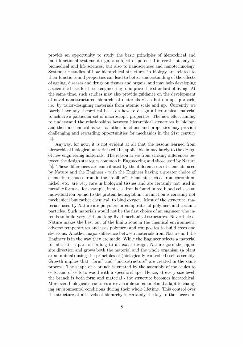
Tendon is based on the same type of collagen fibrils as bone, with thedifference that tendon is not normally mineralized (with some notable ex-ceptions, like the mineralized turkey leg tendon). Collagen fibrils in tendonshave a diameter of typically a few hundred nanometers and are decoratedwith proteoglycans, which form a matrix between fibrils (Fig. 1.5b and c).Fibrils are assembled into fascicles and, finally, into a tendon (Fig. 1.5a).

The outstanding mechanical properties of tendons are due to the opti-mization of their structure (see Fig. 1.5) on many levels of hierarchy. One ofthe challenges is to work out the respective influence of these different lev-els. A sketch of the stres–strain curve of tendon is shown in Fig. 1.6. Mostremarkably, the stiffness increases with strain up to an elastic modulus inthe order of 1–2 GPa. The strength of tendons is typically around 100 MPa.Moreover, tendons are viscoelastic and their deformation behavior dependson the strain rate as well as on the strain itself. The maximum strain reachesvalues in the order of 8–10% for slow stretching. In vivo, it is very likely

13

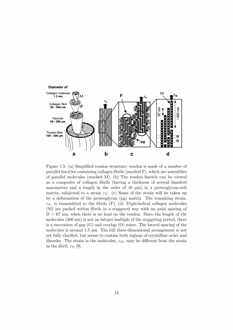
Figure 1.5: (a) Simplified tendon structure: tendon is made of a number ofparallel fascicles containing collagen fibrils (marked F), which are assembliesof parallel molecules (marked M). (b) The tendon fascicle can be viewedas a composite of collagen fibrils (having a thickness of several hundrednanometers and a length in the order of 10 µm) in a proteoglycan-richmatrix, subjected to a strain εT . (c) Some of the strain will be taken upby a deformation of the proteoglycan (pg) matrix. The remaining strain,εF , is transmitted to the fibrils (F). (d) Triple-helical collagen molecules(M) are packed within fibrils in a staggered way with an axial spacing ofD = 67 nm, when there is no load on the tendon. Since the length of themolecules (300 nm) is not an integer multiple of the staggering period, thereis a succession of gap (G) and overlap (O) zones. The lateral spacing of themolecules is around 1.5 nm. The full three-dimensional arrangement is notyet fully clarified, but seems to contain both regions of crystalline order anddisorder. The strain in the molecules, εM , may be different from the strainin the fibril, εF [9].

14

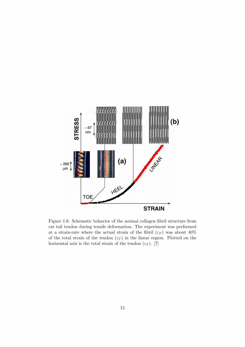
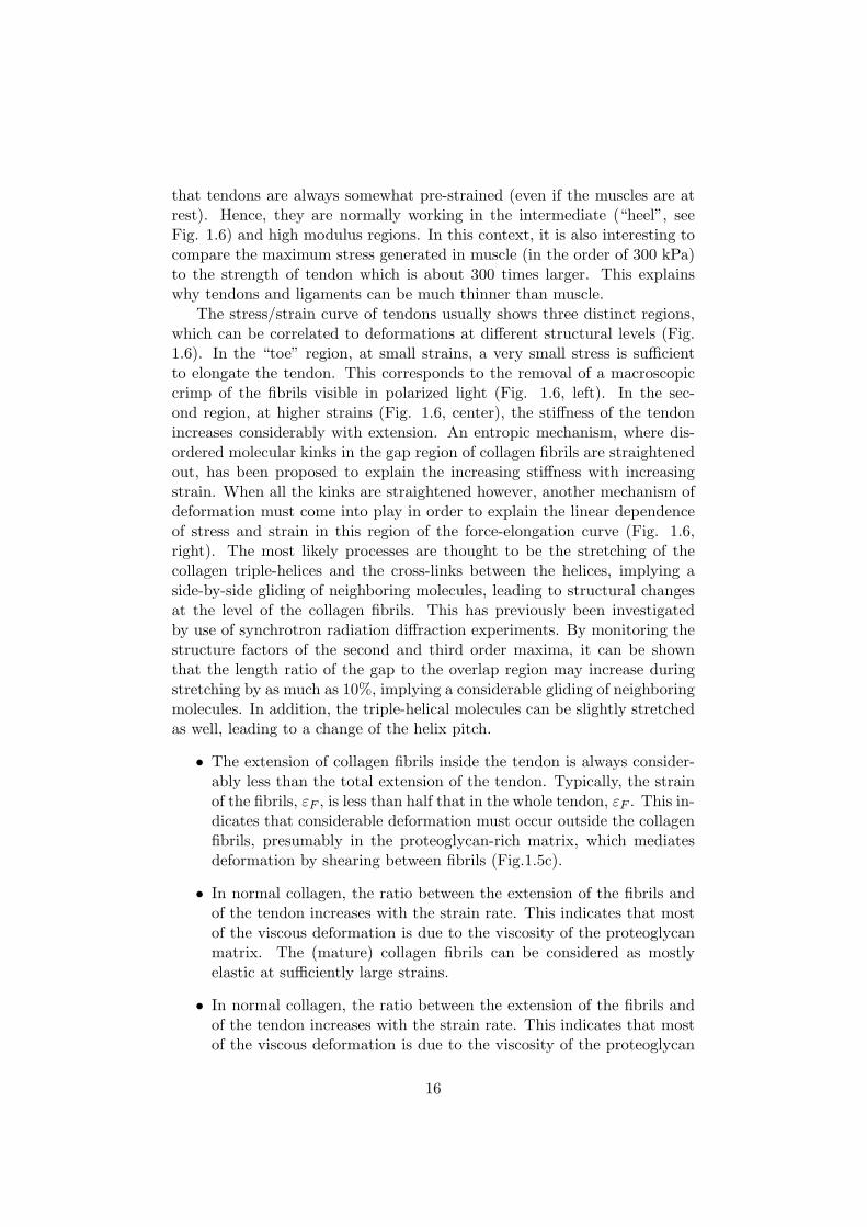
Figure 1.6: Schematic behavior of the normal collagen fibril structure fromrat tail tendon during tensile deformation. The experiment was performedat a strain-rate where the actual strain of the fibril (εF ) was about 40%of the total strain of the tendon (εT ) in the linear region. Plotted on thehorizontal axis is the total strain of the tendon (εT ). [7]

15

that tendons are always somewhat pre-strained (even if the muscles are atrest). Hence, they are normally working in the intermediate (“heel”, seeFig. 1.6) and high modulus regions. In this context, it is also interesting tocompare the maximum stress generated in muscle (in the order of 300 kPa)to the strength of tendon which is about 300 times larger. This explainswhy tendons and ligaments can be much thinner than muscle.

The stress/strain curve of tendons usually shows three distinct regions,which can be correlated to deformations at different structural levels (Fig.1.6). In the “toe” region, at small strains, a very small stress is sufficientto elongate the tendon. This corresponds to the removal of a macroscopiccrimp of the fibrils visible in polarized light (Fig. 1.6, left). In the sec-ond region, at higher strains (Fig. 1.6, center), the stiffness of the tendonincreases considerably with extension. An entropic mechanism, where dis-ordered molecular kinks in the gap region of collagen fibrils are straightenedout, has been proposed to explain the increasing stiffness with increasingstrain. When all the kinks are straightened however, another mechanism ofdeformation must come into play in order to explain the linear dependenceof stress and strain in this region of the force-elongation curve (Fig. 1.6,right). The most likely processes are thought to be the stretching of thecollagen triple-helices and the cross-links between the helices, implying aside-by-side gliding of neighboring molecules, leading to structural changesat the level of the collagen fibrils. This has previously been investigatedby use of synchrotron radiation diffraction experiments. By monitoring thestructure factors of the second and third order maxima, it can be shownthat the length ratio of the gap to the overlap region may increase duringstretching by as much as 10%, implying a considerable gliding of neighboringmolecules. In addition, the triple-helical molecules can be slightly stretchedas well, leading to a change of the helix pitch.

• The extension of collagen fibrils inside the tendon is always consider-ably less than the total extension of the tendon. Typically, the strainof the fibrils, εF , is less than half that in the whole tendon, εF . This in-dicates that considerable deformation must occur outside the collagenfibrils, presumably in the proteoglycan-rich matrix, which mediatesdeformation by shearing between fibrils (Fig.1.5c).

• In normal collagen, the ratio between the extension of the fibrils andof the tendon increases with the strain rate. This indicates that mostof the viscous deformation is due to the viscosity of the proteoglycanmatrix. The (mature) collagen fibrils can be considered as mostlyelastic at sufficiently large strains.

• In normal collagen, the ratio between the extension of the fibrils andof the tendon increases with the strain rate. This indicates that mostof the viscous deformation is due to the viscosity of the proteoglycan

16

matrix. The (mature) collagen fibrils can be considered as mostlyelastic at sufficiently large strains.

Recent modeling work suggests that the design of collagen fibrils in a stag-gered array of ultralong tropocollagen molecules provides large strength andenergy dissipation during deformation. The mechanics of the fibril can beunderstood quantitatively in terms of two length scales, which characterizewhen, firstly, deformation changes from homogeneous intermolecular shearto propagation of slip pulses, and when, secondly, covalent bonds within thetropocollagen molecules start to fracture. Single molecule experiments on(type I) collagen molecules employing atomic force microscopy or opticaltweezers and fitting the data with a worm-like chain model, resulted in apersistence length of about 15 nm, a value close to the predictions of atom-istic simulation of (type XI) collagen molecules. These results confirm thatcollagen molecules are flexible rather than rigid, rod-like molecules.

1.2.3 Spider silk

Spider capture silk is a natural material that outperforms almost any syn-thetic material in its combination of strengthand elasticity. The structureof this remarkable material is still largely unknown, because spider-silk pro-teins have not been crystallized. Capture silk is the sticky spiral in the websof orb-weaving spiders. The major protein of these threads is flagelliformprotein, a variety of silk fibroin.

The spider’s capture silk has tensile strength of ∼ 1 GPa, comparable instrength to Kevlar1 or steel.Unlike those two man-made materials, however,spider capture silk is also extremely elastic and stretches as much as 500–1000% [10]. Stretchy proteins are particularly interesting from a materialspoint of view, given the value of elasticity in the design of fabrics, coatings,ropes and fibers, and structural materials. Some strtchy proteins, such aselastin, stretch and relax without any net enrgy dissipation. This proteinsare highly resilient. Othe stretchy proteins dissipate energy as heat in theprocess of stretching and relaxing and are thus less resilient. One advantageof this is that there is less rebound when the elastic protein relaxes. This isdesirable in spider capture silk, because excessive rebound would propel theinsect away from the web, as if it were on a trampoline.

The two models presented in the following show very clearly how themacroscopic mechanical properties of materials rely on the underlying molec-ular structure.

First model: silk from the synthetic protein pS(4+1).

This model tries to give a description of a soluble synthetic protein fromdragline silk, pS(4+1). This protein provides a test system for establishing

17

the relationships between protein structure and mechanical properties inspider silk.

Spider dragline silk can be pictured as a composite material consisting ofa semiamorphous matrix filled with tiny (< 10 nm) nano-crystalline-like par-ticles. The amino acid (aa) sequence for spider dragline silk proteins is com-prised of poly(A) [poly-(alanine)], for some silks substituted by poly(GA)[poly(glycy-alanine)], and glycine-rich sequences. The 4- to 10-residue-longpoly(A) and poly(GA) motifs are thought to be involved in the formation ofβ-sheet nano-crystalline-like particles. Glycine-rich sequences are thought tofold into some non-α-helical helical structure for GGX 1 or into β-turns forGPGGX, thus forming the semiamorphous matrix. On the other hand, atleast part of these glycine-rich motifs can probably fold into β-sheets and/orform an interphase between crystalline-like objects and a semiamorphousmatrix. NMR and x-ray diffraction experiments show that the crystalline-like particles are well oriented along the silk fiber with polypeptide chainsparallel and alanine residues perpendicular to the fiber axis. These find-ings suggest that protein molecules are overall well oriented in the silk fiber.This high degree of molecular orientation, together with structural organi-zation of dragline silk proteins, is a prerequisite for the unique mechanicalproperties of the whole silk fiber [11].

Two consensus sequences, SPI and SPII, represent major repetitive ele-ments from spider dragline silk proteins The SPI sequence consists of 38 aaand includes 16-aa-long poly(A) and poly(GA) stretches, flanked on bothsides with a total of 22 aa forming glycine-rich GGX motifs. The SPIIsequence consists of a 12 aa representing two GPGGX motifs (fig 1.7).

Almost two thirds of the secondary structure of (SPI)n modular proteinsis made of β-sheets and the rest is mostly β-turns or similar structures withno significant amount of α-helical structure. This observation is in goodagreement with data obtained previously on native spider dragline silk fibersand suggests that recombinant synthetic modular SPI/SPII proteins have astructural organization very similar (if not identical) to native dragline silkproteins. The protein in fig 1.7 has the formula [(SPI)4 + SPII]4, denoted forbrevity pS(4+1). This protein naturally organizes in nanofibers, as shownin fig. 1.8.

The pS(4+1) nanofiber morphology, as well as its mechanical unfold-ing pattern, can be explained by the model in Fig. 1.9. In this model,a single pS(4+1) protein molecule folds into a well defined structure inwhich β-strands of poly(A/GA) sequences in SPI modules form four H-bond-stabilized β-sheets (Fig. 1.9A). These β-sheets alternate with thenon-β (GGX)n sequences of the SPI modules, which form random coils ornon-α-helices.

1(GGX)n denotes repeating aa sequences glycine-glycine-X, where X is usally leucine,tyrosine or glutamine, represented as loose or tight spirals in fig 1.9A and B

18

Figure 1.7: The sequence of pS(4+1) recombinant silk protein, with selectedSPI and SPII modules identified, as well as poly(A/GA) sequences and(GGX)n sequences. N’ and C’ indicate the N-terminal and C-terminal aminoacids respectively [11].

19

Figure 1.8: Silk nanofibers formed from pS(4+1) silk protein deposited onmica; AFM height images. (A) pS(4+1) silk protein is present primarily asaggregates of nanofibers. (B and C) Close-up AFM images of the pS(4+1)nanofibers show segmented substructure. Fat arrows indicate isolated blobsthat are predicted to be segments of nanofibers, based on their sizes. Thinarrows indicate bulges, which often occur at branch points on nanofibersand may be due to nanofibers overlapping. [11]

20

Figure 1.9: A model for pS(4+1) silk nanofiber organization. (A) Thesingle pS(4+1) protein molecule’s polypeptide chain folds into a flat slab-like structure in which four hydrophobic β-sheets of poly(A/GA) (zig-zags)are separated by hydrophilic non-α-helical GGX structures (spirals). Fourpoly(A/GA)-strands form each of the β-sheets that compose the crystalline-like structures of spider dragline silk. The (GGX)n sequences are randomcoils or helices or other non-α-helical helical structures. (B) Approximately30 of these slab-like molecules form a “stack” or “nanofiber segment” be-cause of hydrophobic interactions between β-sheets in aqueous environment.These nano-fiber segments are thought to bind to each other through specific“fiber- forming” signals/structures at their ends. Alternate segment mod-els show either perfect or imperfect (staggered) alignment. (C) The wholepS(4+1) protein nanofiber can be viewed as a chain of segments with eachsegment representing a single pS(4+1) protein “stack” [11].

21

These folded molecules have the shape of an elongated slab with a patternof alternating hydrophobic and hydrophilic regions formed by β-sheets andby non-β (GGX)n regions, correspondingly. Each slab is a single pS(4+1)molecule, as in Figs. 1.7 and 1.9A . The calculated dimensions of a slab are∼ 0.54 nm high × 2 nm wide × 40 nm long. The height and width comefrom the spacing between typical antiparallel β-sheets (estimated as 0.53–0.55 nm) and the interchain distance along the H-bond direction (estimatedas 0.47 nm). The length comes from the length of four folded SPI domains,calculated from their amino acid sequences [0.32–0.35 nm/aa in β-strandpoly(A/GA) and ∼0.2 nm/aa in non-α-helical (GGX)n sequences]. Thecalculated length of the slabs–∼ 40 nm– is close to the measured segmentlength in AFM images of pS(4+1) silk nanofibers, which is 35± 9 nm.

In an aqueous environment, these molecular slabs will tend to aggregate,because of intermolecular hydrophobic interactions between their β-sheets.This aggregation is modeled in Fig. 1.9B as a stack of pS(4+1) molecularslabs. The silk protein molecules are aligned along the axis of the β-strands,as is known from NMR and x-ray diffraction. In the diagram of Fig. 1.9B,these stacks are six slabs high and five slabs wide, based on the dimensionsand estimated molecular weight of nanofiber seg ments in AFM images (Fig.1.8 B and C). Because of strong and uniform hydrophobic interactions andH-bonds, the β-sheets in these slabs will form crystalline three-dimensionalstructures like those found in native spider dragline silks. The H-bondsbetween β-strands in a β-sheet (and the hydrophobic interactions betweenβ-sheets to a lesser degree) can be viewed as the major stabilizing forces insuch structures. The ends of each stack seem to carry signals/structures thatfacilitate pS(4+1) nanofiber formation. Thus, it is likely that each nanofibersegment corresponds to a separate pS(4+1) stack (Fig. 1.9 B and C). Thedraw-down process, occurring as one of the last steps in a silk fiber pro-duction pathway, causes major structural rearrangements in silk proteins,resulting in a significant improvement in the fiber mechanical strength. Dur-ing this draw-down step, the glycine-rich part of silk proteins can partiallytransition from random coil or non-α-helical to the more extended struc-tures, such as 31-helix or β-strand. Similar structural rearrangements occurin the silk fibers when they are under a force load.

Spider dragline silk, like lustrin in abalone shell and titin in muscle, thusappears to derive much of its combination of strength and toughness fromits modular sacrificial bonds. Detailed structural and mechanical studies onspider dragline silk proteins should be performed in the future and, for now,this model remains highly speculative.

Second model: spider dragline silk

After conducting observations of spider dragline silk, it can be noted that,the silk thread, having a diameter of 4–5 µm, consists of a number of silk fib-

22

rils with diameter 40–80 nm. According to AFM images, a silk fibril is not acylindrical fibril but some of its segments are interlinked with each other. Asthe imaging of AFM is based on the force profile, segments represent the re-gions that may have harder materials, such as protein polypeptide networksthat are interlinked by rather soft or flexible polypeptide chains. In themodel shown in Fig. 1.10 several β-sheets (crystalline domains) connectedby non-β-structure (noncrystalline domains) form one silk fibril segment (asindicated by the dashed circle, Fig. 1.10, b and c). Many of these silkfibril segments are interlinked with each other, so as to compose one singlesilk fibril along the silk thread axis. The size and orientation of the crys-tallites as well as the intercrystallite distance within the silk fibril can bedetermined by x-ray diffraction. This allows us to establish the correlationbetween the structure and the mechanical properties of the silk obtained atdifferent reeling speeds [12].

The formation of β-sheet crystallites is controlled by nucleation andgrowth processes. The study of the silk secretion of Bombyx mori andNephila clavipes when the silk secretion is put on a glass slide indicatesthat a liquid crystalline phase occurs quickly followed by a slow formationof the crystalline phase. This suggests that the amorphous-to-crystallinephase transition much depends on the initial concentration and subsequentdrying rate, i.e., supersaturation of the silk protein solution. Before the silkis extruded, it passes through a long thin duct. The shearing of the fluid inthe duct compels the protein chains to extend in the direction of the flow,and compels them to come closer to each other. This process increases theconcentration (supersaturation) of the protein chain. When the silk is ex-truded at the spinneret orifice, the supersaturation increases rapidly withevaporation. It has been found that, up to a reeling speed of the silk of∼ 10 mm/s, the higher the reeling speed, the larger the distance betweenthe crystallites along both the meridional and equatorial directions. Thisis because the amorphous chains are in a relaxed state and loosely packedat low reeling speed. When the silk is stretched at high speed, the chainsare easily extended in the direction of fiber axis under high shearing force.Consequently, the intercrystallite distance becomes larger. When the silk isstretched at still higher reeling speed (> 10 mm/s), the silk fibril segmentsstart merging together while the diameter of the silk thread drops an hollowregions begin to appear. Hence the distance between crystallites decreases(Fig 1.11)

It is interesting to find that Young’s modulus and the yield stress attaintheir maximum values at the same reeling speed (increased ∼10 times forYoung’s modulus and 7 times for yield stress at 10–20 mm/s compared withthose at 1 mm/s). This may imply a direct relationship between crystalliteorientation and Young’s modulus/yield stress. The yield stress appears toincrease substantially linearly with increasing orientation. Moreover, thebreaking stress increases with increasing degree of orientation as well. The

23

Figure 1.10: Hierarchical structure of spider dragline silk N. pilipes. (a) SEMimage of spider dragline silk. Scale bar, 1 mm. (b) AFM image showing thesilk fibril structure as the dashed lines indicate. Each silk fibril is composedof interconnected “silk fibril segments” as indicated by the dashed circleof size 40–80 nm. (c) Model for the silk fibril structure: the “silk fibrilsegment” consists of several β-sheets connected by random coil or α-helixforming a protein polypeptide chain network. The mesh size of the networkis the intercrystallite distance. (d) The crystallites in silk fibril have a β-sheet structure. The crystallite size and orientation can be determined byx-ray diffraction. (e) Unit cell of silk crystallite has an antiparallel β-sheetconfiguration. (Dashed lines indicate the hydrogen bonds between proteinchains within one β-sheet.) [12]

24

Figure 1.11: Topographic AFM image of spider dragline silk N. pilipes atdifferent reeling speeds and the proposed model for the corresponding struc-ture change with increasing reeling speed: (a) at 2.5 mm/s, (b) at 25 mm/s,and (c) at 100 mm/s. The direction of thread is indicated by the arrow.(d) At low reeling speed (<2 mm/s, crystallites are less well- oriented andthe amorphous chains are relaxed. (e) With increasing reeling speed, thecrystallites are smaller and better oriented. At the same time, the inter-crystallite distance becomes larger. (f) Further increase of the reeling speed(>10 mm/s) causes nanofibrils to merge further together, and the observed“particle size” as indicated by a dashed circle becomes larger, thus the dis-tance between the crystallites becomes smaller. [12]

25

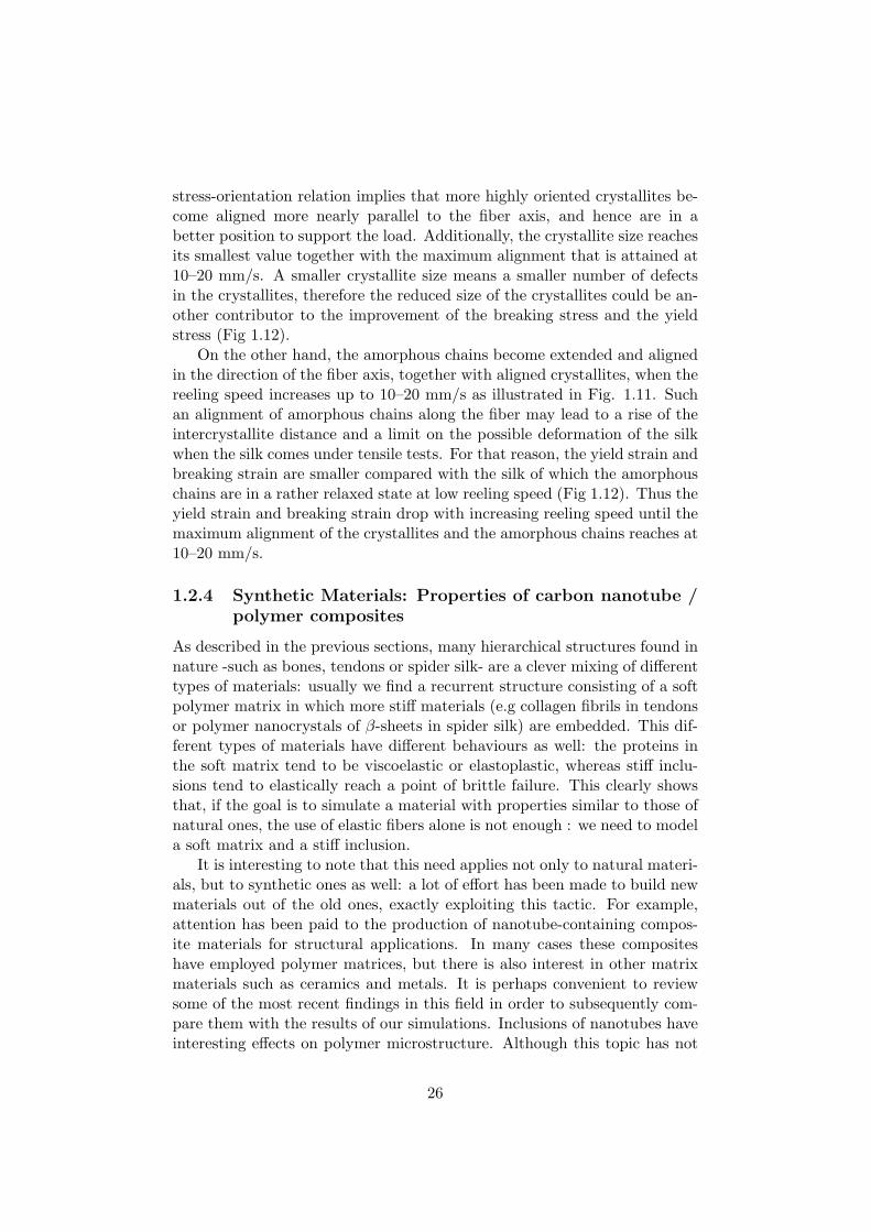
stress-orientation relation implies that more highly oriented crystallites be-come aligned more nearly parallel to the fiber axis, and hence are in abetter position to support the load. Additionally, the crystallite size reachesits smallest value together with the maximum alignment that is attained at10–20 mm/s. A smaller crystallite size means a smaller number of defectsin the crystallites, therefore the reduced size of the crystallites could be an-other contributor to the improvement of the breaking stress and the yieldstress (Fig 1.12).

On the other hand, the amorphous chains become extended and alignedin the direction of the fiber axis, together with aligned crystallites, when thereeling speed increases up to 10–20 mm/s as illustrated in Fig. 1.11. Suchan alignment of amorphous chains along the fiber may lead to a rise of theintercrystallite distance and a limit on the possible deformation of the silkwhen the silk comes under tensile tests. For that reason, the yield strain andbreaking strain are smaller compared with the silk of which the amorphouschains are in a rather relaxed state at low reeling speed (Fig 1.12). Thus theyield strain and breaking strain drop with increasing reeling speed until themaximum alignment of the crystallites and the amorphous chains reaches at10–20 mm/s.

1.2.4 Synthetic Materials: Properties of carbon nanotube /polymer composites

As described in the previous sections, many hierarchical structures found innature -such as bones, tendons or spider silk- are a clever mixing of differenttypes of materials: usually we find a recurrent structure consisting of a softpolymer matrix in which more stiff materials (e.g collagen fibrils in tendonsor polymer nanocrystals of β-sheets in spider silk) are embedded. This dif-ferent types of materials have different behaviours as well: the proteins inthe soft matrix tend to be viscoelastic or elastoplastic, whereas stiff inclu-sions tend to elastically reach a point of brittle failure. This clearly showsthat, if the goal is to simulate a material with properties similar to those ofnatural ones, the use of elastic fibers alone is not enough : we need to modela soft matrix and a stiff inclusion.

It is interesting to note that this need applies not only to natural materi-als, but to synthetic ones as well: a lot of effort has been made to build newmaterials out of the old ones, exactly exploiting this tactic. For example,attention has been paid to the production of nanotube-containing compos-ite materials for structural applications. In many cases these compositeshave employed polymer matrices, but there is also interest in other matrixmaterials such as ceramics and metals. It is perhaps convenient to reviewsome of the most recent findings in this field in order to subsequently com-pare them with the results of our simulations. Inclusions of nanotubes haveinteresting effects on polymer microstructure. Although this topic has not

26

Figure 1.12: Effect of the reeling speed on the mechanical property of spiderdragline silk. (a) The effect on stress. (b) The effect on strain. [12]

27

yet been widely studied, a number of groups have demonstrated that thecrystallization and morphology of the polymers can be strongly affected bysmall additions of nanotubes. it has been found (2006) that arc-producedMWNTs increased the crystallinity of PVA. Fig. 1.13 shows HRTEM im-ages with well resolved PVA lattice fringes oriented parallel to the nanotubeaxes. Nanotube-induced crystallization has also been observed in a num-ber of other polymers, and may be an important factor in determining theproperties of composites.

The first studies of the mechanical properties of nanotube/polymer com-posites were carried out in 1999, with pretty poor results. The tensile elasticmoduli of the composite films were assessed as a function of nanotube load-ing and temperature. For the theory developed for short-fibre composites,a nanotube elastic modulus of 150 MPa was obtained from the room tem-perature experimental data. This low value may have more to do with poorstress transfer than with the weakness of the nanotubes themselves. Abovethe glass transition temperature of the polymer (∼ 85 C), the nanotubeshad a more significant effect on the properties of the composite.

Rather better results were achieved in 2002 with composites made fromPVA and arc-produced MWNTs. The composites were prepared by solution-mixing and films were formed on glass substrates by drop casting. Thepresence of 1 wt% of nanotubes increased the Young’s modulus and hardnessof a PVA by factors of 1.8 and 1.6 respectively. This improvement over theearlier results reflects both the superior quality of the tubes and strongerinterfacial bonding. Evidence for the latter was provided by TEM studies,and in more recent works a 4.5-fold increase in the Young’s Modulus ofa PVA with the addition of carbon nanotubes was reported. It was foundthat the enhancement of the Young’s modulus was partly due to a nonatube-promoted increase in polymer crystallinity.

The mechanical properties of nanotube/polystyrene composites were stud-ied in the year 2000 as well. During the experiments two samples of catalytically-produced MWNTs were used, one with an average length of ∼ 15µm, theother with an average length of ∼ 50µm. With the addition of 1% of nan-otubes by weight they achieved a 36% and 42% increase in the elastic stiffnessof the polymer for short and long tubes respectively (the neat polymer mod-ulus was ∼ 1.2 GPa). In both cases a 25% increase in the tesile strength wasobserved. Theoretical calculations, carried out assuming a nanotube mod-ulus of 450 GPa, produced increases of a 48% and 62% in the stiffness ofthe polymer for short and long tubes. The close agreement, within ∼ 10%,between the experimental data and the theoretically predicted compositemoduli indicated that the external tensile loads were succesfully transmit-ted to the nanotubes across the tube-polymer interface. At higher nanotubeconcentrations, the changes in the mechanical properties of the compositeswere more pronounced. For MWNT/polystyrene composites containing fron2.5% to 25vol.% nanotubes, Yoiung’s modulus increased progressively from

28

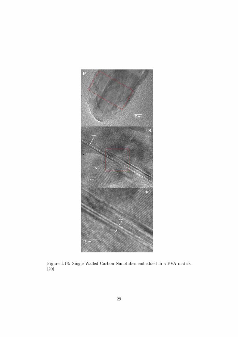
Figure 1.13: Single Walled Carbon Nanotubes embedded in a PVA matrix[20]

29

1.9 to 4.5 GPa, with the major increases occurring when the MWNT contentwas at or above about 10 vol.% However, the dependence of tensile strengthon nanotube concentration was more complex. At the lower concentrations(≤ 10 vol.%), the tensile strength decreased from the neat polymer value of∼ 40MPa, only exceeding it when the MWNT content was above 15 vol.%.

In a 2007 study of nanotube-reinforced polyethylene, the Young’s mod-ulus and tensile strength were found to increase by 89% and 56%, respec-tively, when the nanotube loading reached 10 wt%. An other study foundthat the tensile modulus of PE fiber was improved from 0.65 to 1.25 GPawith the addition of 5 wt% SWNT. Excellent results were also reported withSWNT/nylon composites: the incorporation of 2 wt% SWNTs produced a214% improvement in elastic modulus and a 162% increase in yield strengthover pure nylon. Perhaps the most impressive mechanical properties wereobserved with the SWNT/PVA fibres: these had Young’s moduli of up to80 GPa, tensile strengths of 1.8 GPa and a very high toughness, suggestingapplications such as bullet-proof vests. Moreover, it has been showed thata kind of SWNT/PVA fibres had excellent shape-memory characteristics.

30

Chapter 2

Elements of FractureMechanics and Statistics

Since in our simulations G has been exploited in order to calculate the energydissipated, some basic concepts are introduced in the following.

2.1 The Energy Release Rate, G

Assume that we have a solid body, acted on by a set of tractions and bodyforces. Assume that this body contains one or more cracks, and that theloads are held constant even if the cracks grow. The tractions t and thebody force b could in this case be scaled by a scalar, Q, such that t = Qtand b = Qb. Q is known as the generalized load with dimension [F]. If thedisplacements would change by δu then the work done by the forces on thebody would be

δU =∫

St · δudS +

∫

Vb · δudV =

∫

SQt · δudS +

∫

VQb · δudV. (2.1)

Since the loads remain fixed, the above could be written as

δU = Qδ

∫

St · δudS +

∫

Vb · δudV

.

This can be simplified by defining a generalized displacement, q, with di-mension [L]

q ≡∫

St · udS +

∫

Vb · udV,

then the work done can be simply written as the product of a force anddisplacement increment,

δU = Qδq. (2.2)

31

Any loading applied to the body may now be represented by a single gen-eralized force Q with corresponding generalized displacement q as sketchedin fig. ....

The generalized force and displacement may also be defined for the caseof prescribed displacements: if we scale the prescribed displacement by au = qu, where q is the generalized displacement with dimension [L], thenthe work done due to an increment of displacement δu = δqu is

δU =∫

St · δqudS +

∫

Vb · δqudV

δU = δq

∫

St · udS +

∫

Vb · udV

.

Defining the generalized force, Q, by

Q ≡∫

St · udS +

∫

Vb · udV,

the work increment is once again given by equation (2.2), U = Qδq.The elastic strain energy density is given by

W =∫ γ

0σijdγij ,

so that the stress can be found from

σij =∂W

∂γij.

The total strain energy of the body is

Ω =∫

VWdV. (2.3)

The increment of strain energy density due to a displacement increment δuproducing a strain increment δγ is δW = σijδγij and thus the increment intotal strain energy is δΩ =

∫V δWdV.

From equations (2.1) and (2.2), in the absence of crack growth the workdone on a solid due to a displacement increment is:

δU = Qδq =∫

St · δudS +

∫

Vb · δudV.

Using indicial notation and replacing ti by σijnj we can write:

δU =∫

SσijnjδuidS +

∫

VbiδuidV.

Applying the divergence theorem to the first of the above integrals we have:

δU =∫

Vσij,jδui + σijδui,j + biδui dV.

32

Applying the equilibrium equation σij,j + bi = 0 and noting that σijδui,j =σijδγij = δW, we get:

δU =∫

VσijδγijdV =

∫

VδWdV = δΩ. (2.4)

Thus we have shown that in the absence of crack growth, the increment ofwork done is equal to the increment in strain energy of the body.

For a prescribed displacement problem the total strain energy will bea function of the displacement, q and of the crack configuration, simplifiedhere as being represented by a crack area s. Thus we can write Ω = Ω(q, s).If the crack does not grow, then the change in strain energy for an incrementδq of displacement is

δΩ =∂Ω∂q

δq.

Knowing from equation (2.4) that δΩ = δU = Qδq we can infer that

Q =∂Ω∂q

, (2.5)

i.e, the generalized force is the derivative of the total strain energy withrespect to the generalized displacement.

To propagate a crack, energy must be supplied to the crack tip. Thisenergy flows to the crack tip through the elasticity of the body and is dissi-pated via irreversible deformation, heat, sound and surface energy.

In the following the energy release rate, G is defined as the energy dissi-pated by fracture per unit new fracture surface area, ds. We will start withtwo specific cases, then develop the general definition of energy release rate.

Let’s consider first the case of prescribed displacement: if the crack isallowed to propagate, increasing the fracture surface area by an amount δs,then the change in strain energy is:

δΩ =∂Ω∂s

δs +∂Ω∂q

δq. (2.6)

As the crack grows, in the case of fixed (during crack growth) displacementsδq = 0, thus

δΩ =∂Ω∂s

δs,

i.e. even though no external work is done on the body during crack growth,the strain energy changes in proportion to the increment of crack area. Theenergy change per unit area is called the energy release rate, G, with unitsof energy per area or [F·L/L2 ], and is defined by

G = −∂Ω∂s

, (2.7)

33

thus the change in total strain energy for an increment δs of crack surfacearea is

δΩ = −Gδs.

It will be shown that G is always positive and hence that the body losesenergy during crack growth. All of the energy dissipated during fractureflows to the crack from strain energy stored in the body prior to fracture.

For the case of prescribed loading q = q(Q, s), and δq will not be zeroduring an increment of crack growth. Substituting eqns. (2.5) and (2.7),eqn (2.6) ca be written as:

δΩ = Qδq −Gδs.

In words, this tells us that change in stored energy equals the energy inputminus the energy dissipated by the fracture. The above can be rewritten as:

δΩ = δ(Qq)− δQq −GδS.

Noting that, in a prescribed loading problem, δQ = 0,

δ(Ω−Qq) = −Gδs,

from which it can be inferred that

G = − ∂

∂s(Ω−Qq) . (2.8)

Before going on with the general loading case, it can be noted that, for abody of surface S, it is possible to divide its boundary into two parts, oneover which tractions are prescribed, St, and one over which displacementsare prescribed, Su, such that S = St ∪ Su. Using the definitions of thegeneralized force and displacement for the case of prescribed loading, andnoting that in this case S = St, eq. (2.8) is

G = − ∂

∂s

[Ω−Q

∫

St · udS +

∫

Vb · udV

]

= − ∂

∂s

[Ω−

∫

St

t · udS +∫

Vb · udV

].

The quantity in square brackets is the potential energy.For the case of prescribed displacement, noting in this case that b = 0

and S = Su, (or∫St

(·)dS = 0), eqn. (2.7) can be written as

G = −∂Ω∂s

= − ∂

∂s

[Ω−

∫

St

t · udS +∫

Vb · udV

].

Denoting the potential energy by Π, we can write:

Π = Ω−∫

St

t · udS +∫

Vb · udV

, (2.9)

34

where the total strain energy, Ω, is defined in equation (2.3), the energyrelease rate can be written in common form as

G ≡ −∂Π∂s

,

i.e. energy release rate is the change of potential energy per unit crack area.This is taken to be the fundamental definition of G. Any other loading,for example loading by a spring or with mixed boundary conditions (loadprescribed on part of the boundary and displacement on other parts) willfall in between the two extreme cases of prescribed loading or prescribeddisplacement.

2.1.1 The Weibull Statistics

Weibull statistics is often used since it was originally derived exactly for casessuch as the failure probability of a chain of several links, or for phenomenasuch as electrical insulation breakdowns, life of electric bulbs, and in general,for cases where the occurence of an event may be said to have occurred inthe object as a whole. The following will clarify the point in a very simpleway [15].

If a variable X is attributed to the individuals of a population, thedistribution function of X, denoted F (x), may be defined as the numberof all the individuals having a X ≤ x, divided by the total number of theindividuals. This function also gives the probability P of choosing at randoman individual having a value of X equal to or less than x, and thus we have:

P (X ≤ x) = F (x).

Any distribution function may be written in the form 1

F (x) = 1− e−ϕ(x). (2.10)

Although this seems to be a complication, the advantage of this formaltransformation depends on the relationship:

(1− P )n = e−nϕ(x).

1This is immediate, if we consider that:

F (x) = 1− e−ϕ(x) =

Z x

−∞f(X)dX,

being f a finite function such thatR∞−∞ f(X)dX = 1. We can then write :

ϕ(x) = − ln

»1−

Z x

−∞f(X)dX

–.

Since 1− R x

−∞ f(X)dX ∈ (0, 1), ϕ(x) is real, ∀ x ∈ (−∞,∞).

35

Let’s assume now to have a chain consisting of several links. If we have found,by testing, the probability of failure P at any load x applied to a single link,and if we want to find the probability of failure Pn of a chain consistingof n links, we have to base our deductions upon the proposition that thechain as a whole has failed, if anyone of its parts has failed. Accordingly, theprobability of nonfailure of the chain, (1−Pn), is equal to the probability ofthe simultaneous nonfailure of all links. Thus we have (1− Pn) = (1− P )n.If then the distribution function of a single link takes the form of equation(2.10), we obtain:

Pn = 1− e−nϕ(x). (2.11)

Equation (2.11) gives the appropriate mathematical expression for the prin-ciple of the weakest link in the chain, or, more generally, for the size effecton failures in solids.

Now we have to specify the function ϕ(x). The only necessary generalcondition this function has to satisfy is to be a positive, nondecreasing func-tion, vanishing at a value xu which is not necessarily equal to zero. Themost simple function satisfying this condition is

(x− xu)m

x0,

so that we can put:

F (x) = 1− e− (x−xu)m

x0 . (2.12)

The only merit of this distribution function is that it is the simplest math-ematical expression in the form of equation (2.10) which satisfies the neces-sary general conditions. It has been prooved that, in many cases, it fits theobsevations better than other distribution functions. Since it is not possi-ble to find any theoretical basis justifying the form of a given distributionof random variables such as strength properties of materials, the only waythat can be undertaken is to choose a simple function, test it empirically,and stick to it as long as none better has been found.

Equation (2.12) can be easily generalized if we consider the probabilityof failure F (σ) for a specimen of volume V under uniaxial stress σ(x), wherex is a point in the volume V , to have the form:

F (σ) = 1− exp−

∫

V

[σ(x)σ0V

]m

dV

, (2.13)

or, equivalently,

F (σ) = 1− exp[−V ∗

(σ

σ0V

)m], (2.14)

where σ0V and m are respectively the Weibull’s scale and shape parameters,and V ∗ is an equivalent volume that refers to a reference (e.g., the maximum)

36

Figure 2.1: Weibull statistics for strength of carbon nanotubes [17]

stress σ in the specimen, defined by comparing Eqs. (2.13) and (2.14). Ifthe specimen is under uniform tension, σ(x) ≡ σ and V ∗ ≡ V.

If we consider, instead of the failure probability of a given volume, thefailure probability of a given surface, then Eqs. (2.13) and (2.14) take theform:

F (σ) = 1− exp−

∫

S

[σ(x)σ0S

]m

dS

(2.15)

and

F (σ) = 1− exp[−S∗

(σ

σ0S

)m]. (2.16)

As the exponents in the previous equations have to be dimensionless, σ0V

and σ0S need to have the anomalous physical dimensions of a stress timesrespectively a volume or a surface raised to 1/m. When considering thefracture of the external wall of nanotubes under nearly uniform tension,the two approaches are identical, since V = St = πDLt, where t is theconstant spacing between two concentric nanotube walls - it is ∼ 0.34 nm,so that we can consider it as constituting the shell thickness- whereas D andL are, respectively, the nanotube diameter and length. Moreover, since weconsider, at least to a first approximation, the applied tension to be uniform,S∗ ≡ S and V ∗ ≡ V. As shown in Fig. 2.1 , experiments carried out ina series of tensile tests have found, when applying the standard Weibullstatistics, that the Weibull modulus reaches a value ∼ 3, but show a verypoor correlation coefficient R2 = 0.67

A better understanding of failure processes occuring in carbon nanotubesmay come from numerical simulations based on molecular mechanics and ab

37

initio quantum mechanics [16]. The existence of a fracture “quantum” hasbeen proposed, with the further hypothesis that even very small defects cancause the failure of a nearly defect-free structure. For example, a singleatomic vacancy in an infinitely large graphene sheet has been calculated toreduce the strength of the sheet by nearly 20% of its ideal strength! Thus,at the nanoscale, even few defects can be responsible for the failure of thespecimen, regardless of its volume or surface. Moreover, if, instead of consid-ering the value the stress σ reaches at each point of the specimen, a criticalfailure threshold is assigned to the stress mean value σ∗ evaluated alongthe fracture quantum, theory agrees in a much more satisfactory way withthe experimental results, as shown in Fig 2.2, with a correlation coefficientR2 = 0.93. Correspondingly, instead of taking into account the volumesand surfaces, as in Eqs. (2.13) and (2.15), the following nanoscale Weibullstatistical distribution has been proposed:

F (σ∗) = 1− exp

−

∑n

[σ∗(n)

σ0

]m

,

which, following the steps in Eqs. (2.14) and (2.16), can be rewritten as

F (σ∗) = 1− exp[−n∗

(σ∗

σ0

)m],

where σ0 and m are two constant, and n∗ can be considered as an equivalentnumber of defects. If we consider the nanotubes to be under uniform tension,σ∗(n) ≡ σ∗ ≡ σ and n∗ ≡ n, where σ is the applied load and n the numberof critical defects. After setting n = 1 and σ0 = 31 GPa , the value m ∼ 2.7has been found. These have been the values used in our simulations.

38

Figure 2.2: Modified Weibull statistics for strength of carbon nanotubes[17].

39

Chapter 3

Carbon Nanotube Bundles

We now turn to the description of the developed computer program, outlin-ing its characteristics and the simulation goals.

3.1 The goals of the simulations

This program was written using Matlab, which has the great advantage tobe a flexible, reliable and easy-to-use programming language.The goal was twofold: firstly, the designing of the most simple model ableto explain some constitutive features of the previously described naturalmaterials: this means that the model should account, for instance, for thehigh strength and toughness of bones, tendons or spider silk; moreover, sincethese materials have developed their properties by choosing a hierarchicalstructure, some kind of hierarchy needs to be implemented in the programas well.Secondly, to analyse the role played by inclusions within and throughoutall levels of hierarchy: by referring to inclusions, we mean that we need toconsider that each level of hierarchy may be made up of different materialswith different mechanical properties. A good example is spider silk, wherestiff nano-crystals are embedded in a matrix polymer: this type of stiffinclusions is one of the key reasons of its toughness and need therefore to bepart of the simulation. Their percentage within the soft matrix, their form,their disposition and their elastic modulus are essential characteristics thathave to be investigated.

As previously reported, the way inclusions are scattered within the softmatrix determines the possible paths cracks follow during their propagation:the longer the crack, the bigger the crack surface area: this implies greateramount of energy needed to create the surface, that is, greater capability ofenergy absorption or, equivalently, enhanced toughness.It is important to underline that the aim was not the exact modelling ofa specific structure among those described in the previous chapter: rather,

40

we focused on the outlining of common characteristics all of them share:namely, hierarchy and presence of inclusions. Moreover, a simple model isnot just a tool good for simplifying a problem while still trying to get a roughunderstanding of the original case, but it can also show how to build newsynthetic materials out of the type of hierarchy introduced in the simulation.In order to clarify this point, we introduce, as an example, the simple modelwe began with and the basic ideas it rests upon.

3.2 The first model: Carbon Nanotubes

The starting point has been the recently carried out study of a highly hy-pothetical space elevator, consisting basically of a very long cable attachedto the Earth’s surface and of the related climbers, similarly to a traditionalelevator [13]. The most critical component, when designing the whole struc-ture, would definitely be the cable, which requires a material with both veryhigh strength and low density. Considering Carbon, the maximum stressreached at the Earth’s geosynchronous orbit would be ≈ 63 GPa: only afterthe discovery of Carbon Nanotubes (CNT) such a large stress failure hasbeen experimentally measured in nanotensile tests on CNTs, which are ex-pected to have an ideal strength of ≈ 100 GPa. It is interesting to remarkthat the maximum expected stress inside the cable in the case of steel wouldbe ≈ 383 GPa, whereas for kevlar it would reach ≈ 70 GPa: these valuesare much higher than their strength (respectively 250 GPa for A36 steel and3.6 GPa for kevlar). However, theoretically, such a cable could be made upof any material whatsoever if, instead of a constant cross-sectional area, weconsider a cross-sectional area varying according to a uniform tensile stressprofile alongside the cable itself. In this case, the important parameter tomonitor would be the taper ratio, that is, the ratio between the maximumcross-sectional area at the geosynchronous orbit and the minimum one atthe Earth’s surface. Problems arise since a giant and unrealistic taper ra-tio would be needed in the case of steel or kevlar, in the order of ≈ 1033

and ≈ 108 respectively, whereas the ratio would only be ≈ 2 in the case ofdefect-free CNTs!

If we temporarily assume the making of such a huge cable (about 100000Km long) possible, it would be important to understand how this couldbe realized out of tiny CNTs, each about 0.7 µm long: hierarchy has topop up in some way, since we span throughout 15 orders of magnitude.The following scheme has been adopted for our simulations as well, and,therefore, it will be described in detail.

The cable is modelled as a Nxk by Nyk ensemble of subvolumes (prac-tically springs), arranged in parallel sections, as shown in figure 3.1. Eachof the primary subvolumes is in turn constituted by Nx(k−1) by Ny(k−1)

secondary subvolumes, arranged in parallel as before. This scheme is re-

41

Figure 3.1: CNTs hierarchical structure

peated k times down to the first level subvolume, which comprises a Nx1

by Ny1 arrangement of springs (or, more generally, of fibers), represent-ing the actual nanotube (Fig 3.1). A scale-invariant approach has beenadopted, whereby the simulated structure appears the same at any givenscale level. (i.e., the length/width ratio is constant), and therefore we chooseNx1 = Nx2 = · · · = Nxk ≡ Nx and Ny1 = Ny2 = · · · = Nyk ≡ Ny. The cableas a whole comprises a total number of nanotubes Ntot = (NxNy)k and, inorder to get close to the estimated number of CNTs in the space-elevator,≈ 1023, the values k = 5, Nx = 40 and Ny = 1000 have been chosen. It isinteresting to remark that this very simple model ressembles very much thehierarchical structure of natural materials such as tendons, where polymericfibre bundles are in turn organized into bigger fibre bundles. At level 1the behaviour of single nanotubes is modelled: a fixed elastic modulus anda failure strength distributed according to the (nanoscale) Weibull densityfunction are assigned to each one, according to observations from nanoten-sile tests. Linearly increasing strains are applied to the fiber bundle, and ateach code iteration the number of fractured fibers is computed (fracture oc-curs when local stress exceeds the nanotube failure strength) and the strainsuniformly redistributed among the remaining intact fibers in each section.Such uniform redistribution is plausible for indipendent nanotubes. Variousquantities are monitored during the simulation: for example, stress-strain,

42

Young’s Modulus, number and location of fractured fibers, kinetic energyemitted, fracture energy absorbed, and so on. The simulation ends whenall fibers in one of the sections become fractured, dividing the cable intotwo pieces: the above procedure is repeated many times in order to obtainreliable statistics for the computed quantities, usually 103 − 104 times foreach level.

The second-level fibers are those characterized in level 1 simulations, thatis, their stiffness and strength distribution are derived from level 1 results.The same is true for level 3 simulations depending on level 2 results, and soon. This means that the elastic modulus and the statistical distribution ofthe failure stress of level i fibers are assigned according to those emergingfrom level i−1 simulations. Again, repeated displacement-controlled virtualexperiments are carried out at each level, with the same procedure as thatoutlined for level 1, leading hierarchically, at level 5, to results for the full-scale space elevator cable. Results for the strength distributions p(σfi) atthe various levels are shown by histograms in Figure 2.

The level 1 distribution (Fig. 3.2) is centered around 15 GPa and ismuch narrower than the assumed distribution for the nanotube strengths,and can be adequately fitted with a Weibull distribution using σ0 = 13.14GPa and m = 36.53 as Weibull parameters (Fig. 3.2a). The latter can bedetermined by introducing the variables Y = ln(− ln(1− P )) and X = ln σand linearly fitting Y with respect to X, with the correlation coefficient ofthe fit taken as the evaluating parameter for the reliability of the fit. The fit-ting parameters allow the determination of σ0 and m as X = m−1Y + lnσ0.The simulations to determine the subvolume strength at level 2 are thusbased on this distribution. Results of repeated simulations are shown ina typical histogram in Fig. 3.2b. The distribution, which is the result ofmore than 104 repeated simulations, is again narrower than those at previ-ous levels, and is centered around 11.13 GPa. In this case, some variationappears in the distribution form, with more than one peak appearing, anda Weibull function no longer correctly describes the dispersion of the data(continuous line in Fig. 3.2b). To avoid this problem, the choice is made touse the actual distribution obtained in level 2 simulations (plotted by thehistograms) as an input for level 3 simulations, that is, the strengths of thelevel 2 subvolumes constituting a level 3 subvolume are randomly selectedfrom the distribution in Fig. 3.2b. The same procedure is adopted in thesimulations

for levels 4 and 5, and results are shown in Fig. 3.2c–e.In each case, a decrease in the mean subvolume strength is noticed with

respect to the previous level, with the main decrease occurring from level 1to level 2 and a further decay in the higher levels. Also, there is a decreasein the dispersion of results, with increasingly narrow distributions. The finalstrength at level 5 can be evaluated at approximately 10.20 GPa, that is,less than 30% of the original mean nanotube strength and reduced to ∼ 10%

43

Figure 3.2: Simulation results for the subvolume strength distribution fromlevel 1 to 5 (a to e, respectively). Only level 1 results can be adequatelyfitted with a Weibull distribution.

44

Figure 3.3: Results of simulations for the rescaled cable strength versuscable length using three different simulation parameters (m) in the assumedWeibull distribution.

of the theoretical nanotube strength.Results are plotted in Fig. 3.3 for σf/σ0 versus subvolume length L.

45

Chapter 4

Elastoplastic Behaviour:Energetic Aspects

The simulations carried out with this program had proved to be extremelyuseful in understanding the behaviour of hypothetical megacables made upof CNTs, in particular in understanding how much defects can affect thestrength of the whole structure. The main characteristics of the the pro-gram were: 1) the first hierarchical level constituted only of totally elasticfibers,whose failure strength was distributed according to the Weibull statis-tics; 2) defects were modelled as holes in the fiber structure: this means thatsome fibers were missing, randomly or clustered in order to shape a greatervacancy with a specific form (Fig. 4.1).

However, if we want to model some different kind of materials, or, moreprecisely, to come closer to more realistic simulations of both natural andsynthetic materials, we need to make a step further and add new ingredients,that is, new parameters in the simulation.

The basic ideas that have been followed are very simple. First of all,we want to study how the crack propagates through a sample made up ofdifferent materials, each one endowed with a different constitutive law. Infact, as previously said, if we want to try to model some aspects of naturalor synthetic materials, and, moreover, if we want to exploit a simple fibrebundle model, as that depicted in Fig. 3.1, then considering only fibers withelastic behaviour is no longer adequate, and we have to add other types offibers with other consitutive laws. In particular, it has been tried to modelmaterials, such as carbon nanotubes/polymer composites, which consist ofmatrices including stiffer inclusion, that is, carbon nanotubes. The modelis depicted in fig. 4.2.

Simulations are carried out in what amounts to the numerical equiv-alent of crack opening displacement control, i.e. the simulation proceedsby fracturing one fibre at a time, based on the respective yield or fracturestrengths and the stresses acting on the fibres, then setting the overall stress

46

Figure 4.1: Defective cable configurations considered in simulations: a-b)circular defect having a width of respectively 1/10th and 1/4th of thespecimen width; c) vertical elliptical defect; d)horizontal elliptical defect; e)distributed circular defects; f) distributed point defects.

Figure 4.2: Schematic representation of mixed fragile-plastic fibre bundlemodel: constitutive laws are shown for fragile (left) and plastic (right) fibres,respectively.

47

and strain to the appropriate values. This gives rise to stress-strain curvesas those pictured in Fig. 2, which include ”softening” phases with recedingstresses and/or strains. The corresponding branches can be captured exper-imentally only by controlling a monotonically increasing variable (e.g. thesoftening with negative slope by controlling the strain) and thus the soft-ening with positive slope (curve for p=0) can be observed only controllingthe crack opening; accordingly, also controlling the strain would lead to aundesired catastrophic failure of the specimen (see Catastrophe Theory).Energetic aspects of the simulated tensile tests are also accounted for. Ateach level, variations in external work ∆W , accumulated elastic energy ∆U ,and dissipated energy ∆Ω in plastic deformation and crack surface forma-tion) are computed for each fibre failure. The external work ∆W is givenby:

∆W = F∆x + x∆F,

where F and x are the applied force and displacement, respectively, and ∆Fand ∆x their variation at the considered loading step. The accumulatedelastic energy ∆U is given by

∆ =12x2∆k + kx∆x,

where ∆k is the variation in the overall bundle rigidity due to the fractureor yielding of the relevant fibre. As mentioned above, the dissipated energyis composed of a contribution due to fragile fibre failure and a contributiondue to the deformation of yielded plastic fibres:

∆Ω = (GcAf )fragile + Af lf

∑

j

σyj

∣∣∆εj

∣∣

plastic

,

whereGc is the material fracture energy, Af the fibre cross-sectional area, lfthe length, σyj the yield stress of the j-th yielded fibre, ∆εj the variationin its strain, and the sum is carried out over yielded fibres only. Finally,energy balance considerations allow the determination of the variation inthe released kinetic energy ∆T (e.g., in stress waves and acoustic emissions)as:

∆T = ∆W −∆U −∆Ω.

First we wish to evaluate the qualitative behaviour of the proposed model.One of the possible applications is to evaluate the influence of the relativevolume fractions of the components on the mechanical behaviour of a carbonnanotube based composite. This is of practical importance for the designof composites with tailor-made properties, as is often required in materialscience. Typical results are shown in 4.3.

It is interesting to notice that in the case of 100% fragile fibres, the spec-imen fractures after a softening phase with positive slope. This corresponds

48

Figure 4.3: Typical level 1 stress-strain curves for varying plastic fibre per-centage p. The catastrophic behaviour (softening with positive slope, p=0)disappears for about p >0.2.

49

to a catastrophic behaviour, i.e. controlling in force or displacement wouldresult in a abrupt failure with large emission of kinetic energy. This unde-sired effect does not occur when a ∼ 20% of plastic fibres are present. Whilethere is little effect on the overall strength of the model specimen, failurestrains increase considerably with p. It is therefore clear that an increasingpercentage of plastic fibres implies a greater energy dissipation. This is dueto the fact that plastic fibres continue to support stresses after yielding, andtherefore continue to dissipate energy when fragile fibres would have ceasedto. This effect is particularly interesting for engineering applications, wherea considerable energy as well as stress is required to bring a specimen tofailure. The effect is indeed exploited in carbon nanotube based composites,modelling the behaviour seen in nature, e.g. in the case of spider silk.

Figure 4.4 illustrates the variation of external work W , elastic energy U ,dissipated energy Ω and released energy T for a typical simulation. It mustbe stressed that the abscissae do not correspond to time, as one would havein a displacement- or force-controlled experiment, rather to a simulation stepthat corresponds to the failure or yielding of a single fibre composing thechain of bundles. It is noticeable that the external work carried out to deformthe specimen is only partially accumulated in elastic energy in the specimenor dissipated due to crack surface formation or plastic deformation. Thismeans that at each fibre fracture part of the remaining energy is releasedin the form of stress waves. As the simulation advances and more andmore plastic fibres reach their yield point, the dissipated energy becomesproportionally more significant, leading to a decrease in released energy.The final part of the simulation, with decreasing W and U , corresponds tothe softening branch of the stress-strain curve.

50

Figure 4.4: Example of energetic analysis for a level 1 simulation up to spec-imen failure: variation of external work (W ), potential elastic energy (U),dissipated energy (Ω), and released energy (T ) as a function of simulationstep number. All energies are expressed per unit mass (in grams).

51

Chapter 5

Hysteresis

5.1 The computer program

To be clear, let’s consider for the moment a fibre bundle model consistingonly of a series of elastic fiber sections, each one piled up on the previous oneas in Fig. 5.1. We assume that we can find out, at least qualitatively, themechanical properties of a material by means of such a simple model: weapply a force F on both ends of the bundle: each section will extend accord-ing to the stiffness of the fibres it is made of. Namely, at the equilibrium,the i-th section will extend according to the obvious law:

F =Nyi∑

j=1

kij xi,

where Nyi is the number of fibres of the i-th section, kij is the stiffness ofthe (i,j)-th fibre, and xi is the deformation of the whole section. We candescribe exactly the same situation by using, instead of F , kij and xi, thetotal stress σ = F

A (being A the cross sectional area of the bundle), the fiberYoung’s modulus Eij = kij l

Af(where l is the fibre length and Af its cross

Figure 5.1: A Fiber Bundle Model of elastic fibres

52

Figure 5.2: Constitutive law of an elastic fibre

sectional area) and the section strain εi = xi/l:

σ =Nyi∑

j=1

Eijεi. (5.1)

We associate to each elastic fibre a failure strength σf according to theWeibull statistic: when the load exerted on the (i,j)-spring reaches its failurestrength σij , then it breaks, that is, it breaks when it is extended up toεf ij = σij/Ei,j . (Fig. 5.2)

We want to study the strength and toughness of a hierarchical material,that is, the force we have to apply before a crack opens and propagates,and the work spent for the propagation to take place. The correspondingprocess we have to analyse, when considering a fibre bundle, is the extensionthe bundle reaches before the breaking of a fibre, and the force needed ateach subsequent step to break another spring anywhere else in the bundle.In this way, a propagating crack is equivalent to many adjacent springs thatbreak one after the other.

If, besides elastic fibres, elasto-plastic ones are considered, then we haveto take into account their effect on the whole bundle. They have a differentconstitutive law: after an elastic part, reached the yield strain εy , they keepelongating at the same applied stress until the failure point εp is reached(Fig. 5.3).

Equation (5.1) needs then to be modified, in order to keep track of theyielded fibres in the section:

F = Af

Nyi∑

j=1

[Eijεi + σyij

], (5.2)

∀ i = 1, . . . , Nx, where σyij are the yield stresses of yielded fibers. If theapplied force F and the σyij are known, i = 1, . . . , Nx, j = 1, . . . , Ny, then

53

Figure 5.3: Constitutive law of an elasto-plastic fibre

we can find out the strain of the i-th section. Having the strain of eachsection of the budle , then we can find the elongation of the whole bundle.

The program is aimed at modelling a crack opening, so that at each stepof the simulation an event occurs. Since the bundle is now made up of bothelastic and elastoplastic fibres, three different events are possible: 1) thebrittle failure of an elastic fibre; 2) the yielding of an elasto-plastic one; 3)the rupture of a yielded fibre. The simulation begins with no force applied.Then the smallest possible force is exerted on the bundle, to induce one ofthe three possible events above. In other words, this corresponds to pullingthe bundle until the weakest fibre either breaks or yields, depending on itsconstitutive law. The problem is to determine the force to apply and whichis the fibre that breaks first.

To begin with, we have to define exactly the characteristics of the fi-bres of the bundle. Depending on the desired percentage of the elastic andelastoplastic fibres, different parameters are assigned to them. Namely:

• if the fibre (i, j) is elastic, the failure strength σf ij , following theWeibull distribution with nominal fracture stress σ0f and Weibullmodulus mf ;

• if the fibre (i, j) is elasto-plastic, the yield strength σyij , and the ulti-mate strain εrij . Both yield strength and ultimate strain are Weibulldistributed, with, respectively, nominal yield stress σ0y and Weibullparameter my and nominal ultimate strain ε0 and Weibull parametermε.

• The state of the fibre has to be known, that is, if it is in the elasticregion, if it has yielded, or if it has already broken. This is done byassigning a number to each fibre, namely 0 for an elastic one, 1 for ayielded one and 2 for a broken one.

54

All these informations are what we need to find out where the first eventtakes place. In fact, we can compute, for each section, the failure (in thecase of an elastic behaviour) or the yield and ultimate (in the case of anelasto-plastic behaviour) strains of the fibres, respectively εf , εy and εr; wethen choose the smallest one. This means that we imagine to pull the sectionuntil an event occurs, at εi,min = minεf ij , εyij , εrij , j = 1 . . . , Ny. Thenthe force needed to reach that point is calculated. At the beginning of thesimulation all fibres are elastic, so we can use equation (5.1):

Fi,min(εi,min) = Af

Ny∑

j=1

Eij εi,min,

i = . . . , Nx. At successive steps, when some fibres have already yielded,

Fi,min(εi,min) = Af

Ny∑

j=1

[Eij εi,min + σyij

].

In this way we have a set of Nx forces, one for each section: each forcerepresents the load to be applied to let the weakest fibre in the sectioneither yield or break. The smallest value in the set is the force to be appliedto the whole bundle, so that only the weakest fibre undergoes a change. Inthis way, we are able to control at each step the cracks taking place and howthey develop. The following graphs show the results obtained for bundlesmade up of different percentages of elastic and elastoplastic fibres. Thenominal failure and yield stresses σ0f and σ0y have been set respectively to34 MPa, and the Weibull parameters mf and my have been set to 2.

There are two aspects to remark: the first, that the overall behaviourof a bundle constituted only of linear elastic fibers, Fig. 5.5, is no longerlinear. The second, that, for bundles made up of half or more elastoplasticfibres (Figgs. 5.7 and 5.8), non-physical stress-strain curves appear. In fact,it is not possible that, after some springs have broken and many more haveyielded, the bundle is stiffer than at the beginning.

The reason is the following: if we consider the strain of each section afterhaving exerted a force F on the bundle, some of them have negative values,as if, when being pulled, they were compressed instead of elongated. Thiscan be understood by looking at the way the strains εi are computed. Fromeq. (5.2), we get:

εi =1

∑Ny

j=1 Eij

F

Af−

Ny∑

j=1

σyij

.

It could then be the case that the contribution of the yielded fibresin a section,

∑Ny

j=1 σyij , is greater than the applied stress FAf

. Since, at

55

0 0.2 0.4 0.6 0.8 1 1.2 1.4 1.6 1.80

0.5

1

1.5

2

2.5

3x 10

8

εin

σ in

Figure 5.4: Stress-strain curve for a bundle made up of 100% elastic fibres

10 20 30 40 50 60 70 80 90 100

5

10

15

20

25

30

35

40

45

50

Figure 5.5: Crack propagation for a bundle made up of 100% elastic fibres.

56

0 0.2 0.4 0.6 0.8 1 1.2 1.4 1.6 1.80

0.5

1

1.5

2

2.5

3x 10

8

εin

σ in

Figure 5.6: Stress-strain curve for a bundle made up of 80% elastic, 20%elasto-plastic fibres

0 0.5 1 1.5 20

0.5

1

1.5

2

2.5

3x 10

8

εin

σ in

Figure 5.7: Stress-strain curve for a bundle made up of 50% elastic, 50%elasto-plastic fibres

57

−0.5 0 0.5 1 1.5 2 2.50

0.5

1

1.5

2

2.5

3

3.5x 10

8

εin

σ in

Figure 5.8: Stress-strain curve for a bundle made up of 50% elastic, 50%elasto-plastic fibres

equilibrium, each section will react with a force equal and opposed to theforce F exerted on the ends of the bundle, such a contribution has to becorrected in some way: otherwise, in case of negative εi, we would haveF < Af

∑Ny

j=1 σyij . Problems get solved if we consider that an elasto-plasticmaterial undergoes a hysteresis cycle (Fig. 5.9): that is, when a fibre elon-gation reduces because of the reduction of the applied force F , then it getselastic again, but its yield point, where σ = σy, changes: its elastic be-haviour is no longer given by σ = Eε, but rather by σ = E(ε− ε0), so thatεy = ε0 + σy

E and σy = E(εy − ε0).

Figure 5.9: Hysteresis loops in case of cyclic softening

58

0 0.002 0.004 0.006 0.008 0.01 0.012 0.014 0.0160

2

4

6

8

10

12

14x 10

9

εin

σ in

Figure 5.10: Stress-strain curve for a bundle made up of 100% elastic fibreswith hysteresis cycles.

0 0.01 0.02 0.03 0.04 0.050

2

4

6

8

10

12

14x 10

9

εin

σ in

Figure 5.11: Stress-strain curve for a bundle made up of 80% elastic fibreswith hysteresis cycles.

59

0 0.01 0.02 0.03 0.04 0.050

2

4

6

8

10

12

14

16

18x 10

9

εin

σ in

Figure 5.12: Stress-strain curve for a bundle made up of 60% elastic fibreswith hysteresis cycles.

0 0.005 0.01 0.015 0.02 0.025 0.03 0.035 0.04 0.0450

2

4

6

8

10

12

14

16

18x 10

9

εin

σ in

Figure 5.13: Stress-strain curve for a bundle made up of 40% elastic fibreswith hysteresis cycles.

60

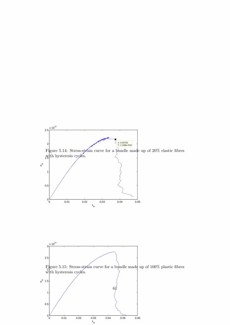
0 0.01 0.02 0.03 0.04 0.050

0.5

1

1.5

2

2.5x 10

10

X: 0.03752Y: 2.158e+010

εin

σ in

Figure 5.14: Stress-strain curve for a bundle made up of 20% elastic fibreswith hysteresis cycles.

0 0.01 0.02 0.03 0.04 0.05 0.060

0.5

1

1.5

2

2.5

3x 10

10

εin

σ in

Figure 5.15: Stress-strain curve for a bundle made up of 100% plastic fibreswith hysteresis cycles.

61

Chapter 6

Percolative CrackPropagation

Two different constitutive laws have been introduced in the model, but,alone, they are not sufficient to describe a real material in terms of fibresand bundles. In fact, if we take tendons as example, even by looking justat the simplified model in Fig. 1.5, it can be seen they are made up ofmaterials, proteoglycan proteins, in which stiffer elastic collagen moleculesare embedded. At the present state, in the simulation, we have elasto-plasticmaterials and elastic ones, but the latter are no stiffer than the first. So whatwe need to do is to draw the geometry of stiff inclusions, analysing how theyare scattered and how this affects the mechanical properties of the bundle.The following figures show some possible choices of the geometry.

Stiff inclusions affect the path cracks can follow through the material:the more staggered inclusions are, the longer the path of the crack. To see it,we can compare the crack path of Fig. 5.5, developed inside a bundle whereno inclusions are present, with that of Fig. 6.3, which is longer because ofthe configuration of inclusions as in Fig. 6.2. The crack is represented bybrown squares, whereas the blue area corresponds to the unbroken fibres;the simulation ends when the crack spans from one side to the other of thebundle.

By looking at Figs 6.7–6.16, it can be noted that, as the number ofplastic fibres within the matrix increases, failure strength and ultimate strainincrease as well, as expected.

62

10 20 30 40 50 60 70 80 90 100

5

10

15

20

25

30

35

40

45

50

Figure 6.1: Parallel inclusions. Their percentage is 20 % of the area of thewhole bundle.

Figure 6.2: Hysteresis loops in case of cyclic softening

63

Figure 6.3: Crack path for a composite with staggered stiff inclusions as inFig. 6.2

0 0.01 0.02 0.03 0.04 0.05 0.06 0.070

2

4

6

8

10

12

14

16

18x 10

9

εin

σ in

Figure 6.4: Stress-Strain curve of a bundle made up of 100% elastic fibersmatrix and 20% inclusions.

64

10 20 30 40 50 60 70 80 90 100

5

10

15

20

25

30

35

40

45

50

Figure 6.5: Crack propagation in the bundle where 100% of fibers in thematrix are elastic: brown squares represent the broken fibres, the blue onesthe intact.

Figure 6.6: Total stress vs time and Total strain vs time for the previousbundle.

65

0 0.01 0.02 0.03 0.04 0.05 0.06 0.07 0.080

0.5

1

1.5

2

2.5x 10

10

εin

σ in

Figure 6.7: Stress-Strain curve of a bundle made up of 80% elastic fibersmatrix and 20% inclusions.

10 20 30 40 50 60 70 80 90 100

5

10

15

20

25

30

35

40

45

50

Figure 6.8: Crack propagation in the bundle where 80% of fibers in thematrix are elastic: brown squares represent the broken fibres, the dark blueones the intact, the light blue the yielded ones.

66

0 0.01 0.02 0.03 0.04 0.05 0.06 0.07 0.08 0.090

0.5

1

1.5

2

2.5

3x 10

10

εin

σ in

Figure 6.9: Stress-Strain curve of a bundle made up of 60% elastic fibersmatrix and 20% inclusions.

10 20 30 40 50 60 70 80 90 100

5

10

15

20

25

30

35

40

45

50

Figure 6.10: Crack propagation in the bundle where 60% of fibers in thematrix are elastic: brown squares represent the broken fibres, the dark blueones the intact, the light blue the yielded ones. It can be seen how the stifferinclusions remain unbroken, whereas the number of yielded fibers increases.

67

0 0.1 0.2 0.3 0.4 0.5 0.6 0.70

2

4

6

8

10

12x 10

10

εin

σ in

Figure 6.11: Stress-Strain curve of a bundle made up of 40% elastic fibersmatrix and 20% inclusions.

10 20 30 40 50 60 70 80 90 100

5

10

15

20

25

30

35

40

45

50

Figure 6.12: Crack propagation in the bundle where 40% of fibers in thematrix are elastic.

68

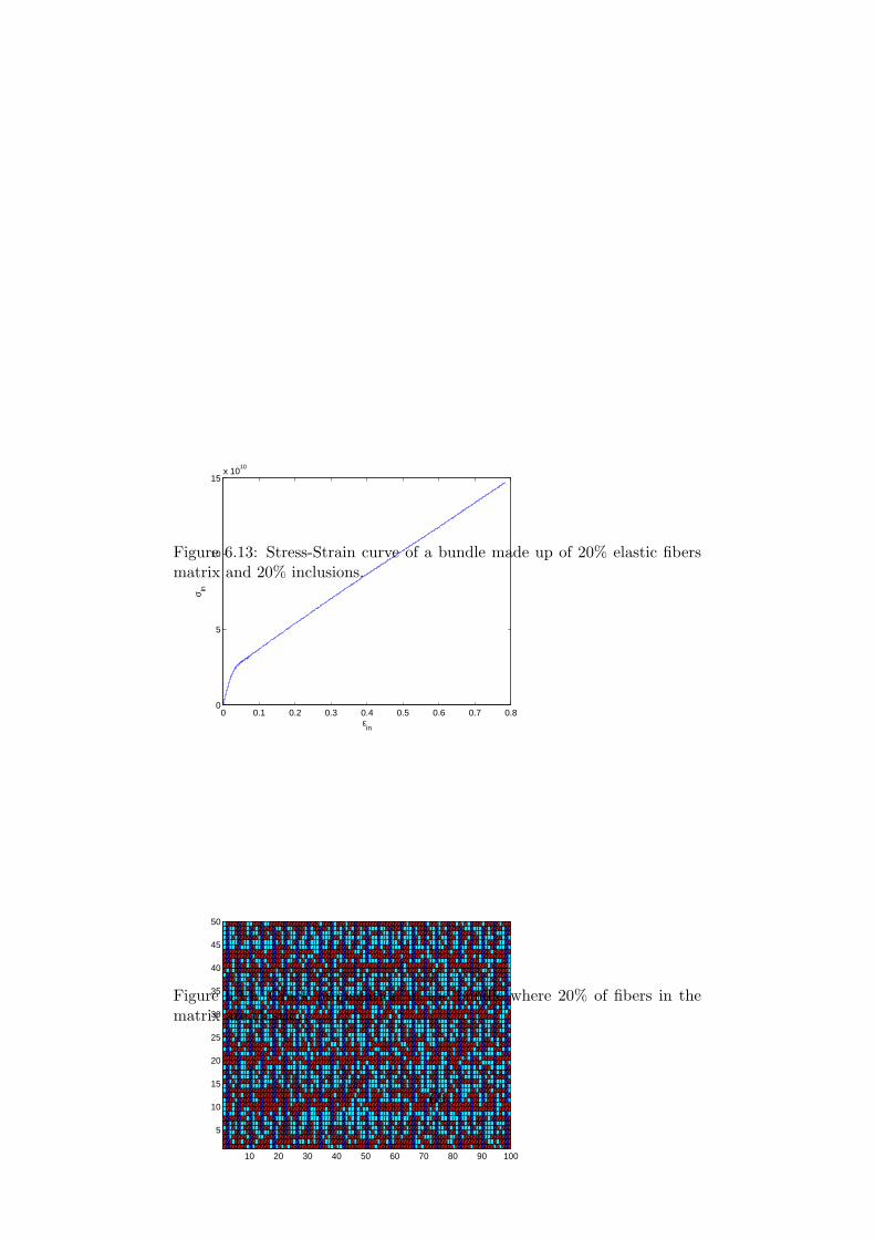
0 0.1 0.2 0.3 0.4 0.5 0.6 0.7 0.80

5

10

15x 10

10

εin

σ in

Figure 6.13: Stress-Strain curve of a bundle made up of 20% elastic fibersmatrix and 20% inclusions.

10 20 30 40 50 60 70 80 90 100

5

10

15

20

25

30

35

40

45

50

Figure 6.14: Crack propagation in the bundle where 20% of fibers in thematrix are elastic.

69

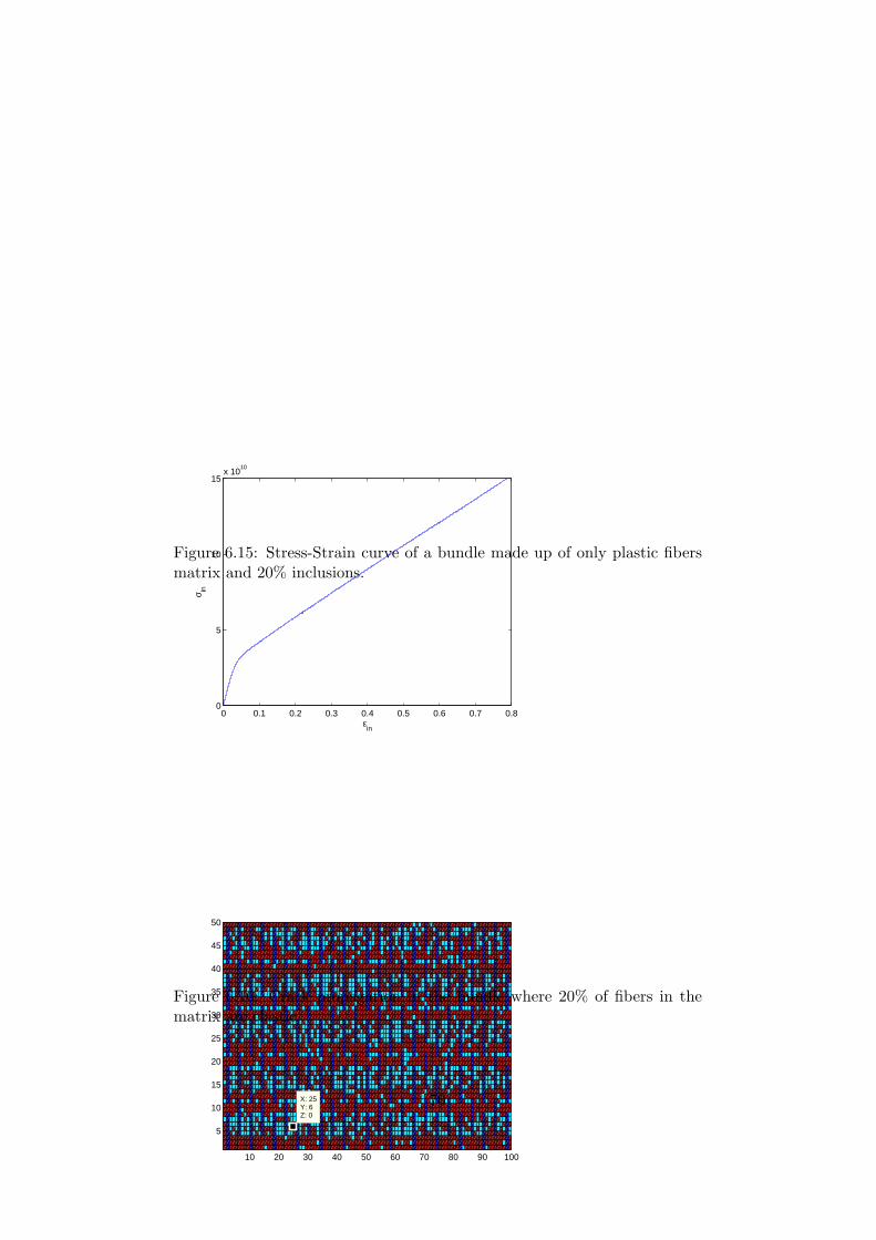
0 0.1 0.2 0.3 0.4 0.5 0.6 0.7 0.80

5

10

15x 10

10

εin

σ in

Figure 6.15: Stress-Strain curve of a bundle made up of only plastic fibersmatrix and 20% inclusions.

10 20 30 40 50 60 70 80 90 100

5

10

15

20

25

30

35

40

45

50

X: 25Y: 6Z: 0

Figure 6.16: Crack propagation in the bundle where 20% of fibers in thematrix are elastic.

70

Chapter 7

An application: the case oftendon fibrils

The computer program has been tested on a real case, to check whetherit can give some results not too far away from experiments. Subsequently,some measures of tendon failure stresses have been carried out in order tocompare them with the obtained numerical results.

We considered, in our simulation, the tendon as consisting of two hier-archical structures, so as to follow the already mentioned model of Fig. 1.5,which we report again.

First of all it is important to correctly define the way inclusions are scat-tered in the first hierarchical level. Contrary to the previously describedmodel, where we have an elasto-plastic matrix and stiff inclusions, the firstlevel of the hierarchy is made up exclusively of elastic fibres, which corre-spond to collagen molecules.

It can be seen from Fig. 7.2 that molecules have a rather fixed struc-ture, where the gap between two molecules in series plus the overlap of two

Figure 7.1: Simplified model of the structure of tendon

71

Figure 7.2: Tendon molecular structure

molecules in parallel amounts to D = 67 nm. In our simulation we setD ∼ 70 nm. The overlap zone is about 40% of D, that is, about 30 nm, thegap zone 60%, that is, about 40 nm.

Moreover, the length of a single molecule is approximately 280 nm,whereas the collagen fibril reaches ∼ 1µm (Fig. 7.3). This means thatone collagen fibril is made up of three collagen molecules in series.

The cross-sectional area of a single collagen molecule, the triple helix ofα-chains, is about 1.5 nm, and the same length distance divides one moleculefrom the other.

In our simulation, we have taken into account these quantities by dividingthe bundle into rectangles and assigning to each one a length of 10 nm anda with of 1.5 nm. This allows to reconstruct, from proper assembly of aninteger number of rectangles, the same structure as in Fig. 7.1. The bundleis composed of 67×96 rectangles (Fig. 8.4). Each molecule chain, depictedin Fig. 8.4 with a specific colour, is monitored. When the chain breaks, itscontribution to the fibril strength vanishes.

72

Figure 7.3: Dimension of the different components of tendon hierarchicallevels [18].

10 20 30 40 50 60

10

20

30

40

50

60

70

80

90

Figure 7.4: Structure of the collagen fibril of Figgs. 7.1c–d as reconstructedin the simulation. Each rectangle corresponds to an area of 10×1.5 nm2.

73

Chapter 8

Experimental results.

Alongside numerical simulations, experiments on deer tendons have beencarried out. Thanks to Professor Bollo and colleagues of the Facolta diVeterinaria of Turin University, Grugliasco, the collection and testing of truetendons has been made possible. Deers that are run over in car accidents aretaken to the Veterinary University for postmortem examination, in order tomonitor the healthiness of the regional deer population. Results from tensileloading experiments on a MTS machine, with precision 1 KgForce are shownbelow. Further Tests will need to be carried out, for a better comparisonwith numerical results.

74

Figure 8.1: Our samples: a deer tendon

Figure 8.2: First Test carried out on a Tendon fiber of ∼ 0.1mm of diameter.

75

Figure 8.3: Other sets of tests: fiber of ∼ 1.5mm of diameter. It was notpossible to break it under 10 N loading.

Figure 8.4: OLast set of measures with another fiber of the same diameterof the previous one. As in the previous case, it has not been possible toreach the breaking point.

76

Bibliography

[1] M. E. Launey, R.O. Ritchie, Adv. Mater. 2009, 21, 2103-2110.

[2] I. Jager, P. Fratzl, Biophys. J 2000, 79, 1737-1746.

[3] B. Ji H. Gao, J. Mech. Phys. Solids 52 (2004) 1963 -1990.

[4] B. Ji H. Gao, Int. J. Frac. (2006) 138, 101-137.

[5] P. Fratzl, R. Weinkamer, Progr. Mat. Sc. 52 (2007) 1263-1334.

[6] J. Aizenberg, V. C. Sundar, A. Yablon, J. Weaver, G. Chen, PNAS,March 9 2004, 101, 10.

[7] P. Fratzl, K. Misof, I. Zizak, G. Rapp, H. Amenitsch, S. Bernstoff, J.Struct. Biol., 1997, 122, 119-122.

[8] J. Aizenberg, J.C. Weaver, M. S. Thanawala, V. C. Sundar, D. E. Morse,P. Fratzl, Science, 2005, 309, 275-8

[9] P. Fratzl, Curr. Opin. Colloid Interface Sci. 2003, 8, 32-9

[10] N. Becker, E. Oroudjev, S. Mutz, J. P. Cleveland, P. K. Hansma, C.Y. Hayashi, D. E. Makarov, H. G. Hansma, Nature Materials, 2003, 2,278-283

[11] E. Oroudjev, J. Soares, S. Arcidiacono, J. B. Thompson, S. A. Fossey,H. G. Hansma

[12] N. Du, X. Y. Liu, J. Narayanan, L. Li, M. Lek Min Lim, D. Li, Biophys.J., 2006, 91, 4528-4535

[13] N. M. Pugno, F. Bosia, A. Carpinteri, small, 2008, 8, 1044-1052

[14] F. Bosia, N. M. Pugno, G. Lacidogna, A. Carpinteri

[15] W. Weibull, J. Appl. Mech., 1951, 293-297

[16] N. M. Pugno, R. S. Ruoff, J. Appl. Phys. 99, 2006

[17] N. M. Pugno, R. S. Ruoff, J. Aer. Engrg, 2007, 97-101

77

[18] M. Buehler, PNAS, 2006,103 33 12285-12290

[19] A. T. Zehnder, Lecture Notes on Fracture Mechanics

[20] M. L. Minus, H. G. Chae, S. Kumar, Polymer, 2006

[21] P. J. F. Harris, Carbon Nanotube Science, Cambridge University Press,2009.

78