universita degli studi di bari - infn.it i am very grateful to ashok kumar (du, india), who have...
TRANSCRIPT

UNIVERSITA DEGLI STUDI DI BARIAldo Moro
Dipartimento Interateneo di Fisica ‘M. Merlin’
Scuola di Dottorato di Ricerca in Fisica
Ciclo XXV
Settore scientifico disciplinare: FIS/01
Background Estimation for the Search of the
Standard Model Higgs Boson in the Decay
Channel H→ ZZ∗ → 4` with the CMSexperiment at
√s = 7 TeV and 8 TeV
Dottorando: Coordinatore:Dott. Gurpreet Singh Chiar.mo Prof. Salvatore Vitale Nuzzo
Supervisore:Chair.mo Giorgio Pietro Maggi Dott. Nicola De Filippis
Esame Finale 2013


To all those who continuously seek the truth . . .


“Our judge is not God or governments, but Nature.”
- Tejinder Singh Virdee


Acknowledgements
I would like to begin by thanking my Ph.D. supervisor, Nicola De Filippis, whose
insistence on expressing problems in the most simplistic terms and enthusiastic sci-
entific attitude, helped me to guide towards the core and fundamental issues of
physics problems. I am extremely grateful for the fundamental and social support,
that I have received from Giorgio Pietro Maggi, who has served as a second advisor
for me. Additionally, I want to thank to Marcello Maggi, who have given numerous
sharp and critical suggestions during my Ph.D. period. I am sincerely thankful to
Lucia Silvestris, Anna Colaleo, Donato Creanza, Alexis Pompili, Director of INFN
Bari, Director of Department of Physics and to the whole CMS Bari community for
their continuos support and cooperation.
I owe the deepest thanks to referees of this thesis: Francesco Conventi (Universita
e INFN Napoli) and Roberto Bellotti (Bari) for their careful reading and valuable
suggestions to improve the quality of my thesis’ content.
I thank Giacinto Donvito for his cooperation and always being available. I also
wish to thank to Anna Massarelli and all members of administrative staff of INFN
and Physics department.
I want to thank all the people for their help and support, who have worked
with me on this analysis or indirectly helped in my work: Joe Bochenek, Marco
Meneghelli, Paolo Giacomelli, Mario Masciovecchio, Cristina Botta, Roberto Salerno,
Adish Vartak, Lorenzo Bianchini, Simranjit Singh Chhibra, Piet Verwilligen.
I am very grateful to Ashok Kumar (DU, India), who have motivated me to join

particle physics and always helped in every possible way.
I want to thank, in particular, the friends who have made my stay a wonder-
ful and memorable in Bari during last three years: Mahinder, Gurpreet Selopal,
Nicola tritto, Francesco Barille, Giacomo, Nicola pacifico, Liliana, Giorgia, Mas-
simo, Mario, Cessare, Rosamaria, Raffaella, Emilia. Finally, I thank to all of my
fellow students, postdocs and all colleagues from Bari and CERN for all of their
support through the years.
I owe the great gratitude to my mother Charanjeet Kaur and my father Wassan
Singh for giving me life and guiding me to where I am today. I thank them and my
younger brother Harpreet Singh for their unconditional love and support.
Last but not least, the Chain of my gratitude would be definitely incomplete if
I would forget to thank the first and the major cause of this chain, The Almighty
“God”. My deepest and sincere gratitude for inspiring and guiding this humble
being.
Gurpreet Singh
February 11, 2013

Contents
Introduction 1
1 The Standard Model 5
1.1 The Standard Model of Elementary Particles . . . . . . . . . . . . . . 5
1.2 The Higgs mechanism . . . . . . . . . . . . . . . . . . . . . . . . . . 7
1.3 Z and Higgs Boson Production in p-p collisions . . . . . . . . . . . . 12
1.3.1 Z boson production . . . . . . . . . . . . . . . . . . . . . . . . 12
1.3.2 Z → 4` process . . . . . . . . . . . . . . . . . . . . . . . . . . 14
1.3.3 Higgs boson production . . . . . . . . . . . . . . . . . . . . . 15
1.3.3.1 Gluon-Gluon Fusion . . . . . . . . . . . . . . . . . . 15
1.3.3.2 Vector Boson Fusion (VBF) . . . . . . . . . . . . . . 17
1.3.3.3 Associated Production . . . . . . . . . . . . . . . . . 17
1.3.3.4 Decay modes of the SM Higgs boson . . . . . . . . . 18
1.4 The SM Background Processes . . . . . . . . . . . . . . . . . . . . . . 19
1.4.1 Irreducible backgrounds . . . . . . . . . . . . . . . . . . . . . 19
1.4.2 Reducible backgrounds . . . . . . . . . . . . . . . . . . . . . . 20
1.4.3 Instrumental backgrounds . . . . . . . . . . . . . . . . . . . . 22
2 Experimental Apparatus 25
2.1 The Large Hadron Collider . . . . . . . . . . . . . . . . . . . . . . . . 25
2.1.1 The LHC design concept . . . . . . . . . . . . . . . . . . . . . 27
2.1.1.1 LHC Collision Detectors . . . . . . . . . . . . . . . . 28
2.1.2 Performance Goals and Constraints . . . . . . . . . . . . . . . 29
2.2 The CMS detector . . . . . . . . . . . . . . . . . . . . . . . . . . . . 31
2.2.1 Inner Tracking System . . . . . . . . . . . . . . . . . . . . . . 34
2.2.1.1 The Silicon Pixel Detector . . . . . . . . . . . . . . . 35
2.2.1.2 The Silicon Strip Tracker . . . . . . . . . . . . . . . 36
2.2.2 Electromagnetic Calorimeter . . . . . . . . . . . . . . . . . . . 37
2.2.2.1 Lead Tungstate Crystals . . . . . . . . . . . . . . . . 39
i

2.2.2.2 Calorimeter Resolution . . . . . . . . . . . . . . . . . 39
2.2.3 The Hadron Calorimeter . . . . . . . . . . . . . . . . . . . . . 40
2.2.4 CMS Magnet . . . . . . . . . . . . . . . . . . . . . . . . . . . 43
2.2.5 The Muon System . . . . . . . . . . . . . . . . . . . . . . . . 44
2.2.5.1 Drift Tube Chambers . . . . . . . . . . . . . . . . . 45
2.2.5.2 Cathode Strip Chambers . . . . . . . . . . . . . . . . 46
2.2.5.3 Resistive Plate Chambers . . . . . . . . . . . . . . . 47
2.2.6 Trigger System and Data Acquisition . . . . . . . . . . . . . . 48
2.2.6.1 The Level-1 Trigger . . . . . . . . . . . . . . . . . . 48
2.2.6.2 The High Level Trigger . . . . . . . . . . . . . . . . 49
2.2.6.3 The Data Acquisition System . . . . . . . . . . . . . 51
2.2.7 CMS Computing Model . . . . . . . . . . . . . . . . . . . . . 52
3 Event Simulation and Reconstruction 55
3.1 Physics Event Generation . . . . . . . . . . . . . . . . . . . . . . . . 55
3.1.1 Hard Scattering Process . . . . . . . . . . . . . . . . . . . . . 56
3.1.2 Parton Shower, Underlying Event and Hadronization . . . . . 56
3.1.3 MC Generator Programs . . . . . . . . . . . . . . . . . . . . . 58
3.1.3.1 PYTHIA . . . . . . . . . . . . . . . . . . . . . . . . 58
3.1.3.2 POWHEG . . . . . . . . . . . . . . . . . . . . . . . 58
3.1.3.3 gg2ZZ . . . . . . . . . . . . . . . . . . . . . . . . . . 59
3.1.3.4 MADGRAPH . . . . . . . . . . . . . . . . . . . . . . 59
3.1.4 K-factors . . . . . . . . . . . . . . . . . . . . . . . . . . . . . . 59
3.2 Detector Simulation . . . . . . . . . . . . . . . . . . . . . . . . . . . . 60
3.2.1 Simulation of Multiple Interactions . . . . . . . . . . . . . . . 60
3.3 Datasets and Triggers . . . . . . . . . . . . . . . . . . . . . . . . . . . 61
3.3.1 Experimental Data . . . . . . . . . . . . . . . . . . . . . . . . 61
3.3.2 Simulated Samples . . . . . . . . . . . . . . . . . . . . . . . . 62
3.3.2.1 Signal: H→ ZZ∗ → 4` . . . . . . . . . . . . . . . . . 63
3.3.2.2 Background: qq → ZZ∗ → 4` . . . . . . . . . . . . . 65
3.3.2.3 Background: gg → ZZ∗ → 4` . . . . . . . . . . . . . 66
3.3.2.4 Background: W/Z+jets→ 2`+jets . . . . . . . . . . . 66
3.3.2.5 Background: tt→ 2`2ν2b . . . . . . . . . . . . . . . 66
3.4 Lepton Selection . . . . . . . . . . . . . . . . . . . . . . . . . . . . . 67
3.4.1 Electron Reconstruction . . . . . . . . . . . . . . . . . . . . . 68
3.4.1.1 Momentum Estimation . . . . . . . . . . . . . . . . . 68
3.4.2 Electron Identification . . . . . . . . . . . . . . . . . . . . . . 69
3.4.2.1 Working Point Optimization . . . . . . . . . . . . . . 71

3.4.3 Muon Reconstruction . . . . . . . . . . . . . . . . . . . . . . . 72
3.4.3.1 Momentum Estimation and Corrections . . . . . . . 73
3.4.3.2 Ghost Muon Removal . . . . . . . . . . . . . . . . . 73
3.4.4 Muon Identification . . . . . . . . . . . . . . . . . . . . . . . . 74
3.4.5 Leptons Isolation . . . . . . . . . . . . . . . . . . . . . . . . . 76
3.4.6 Pile up Corrections . . . . . . . . . . . . . . . . . . . . . . . . 77
3.5 Studies about the MC Simulation . . . . . . . . . . . . . . . . . . . . 79
3.5.1 Key Observables from MC Simulation . . . . . . . . . . . . . . 80
4 Event Selection & Background Control 85
4.1 General Event Selection . . . . . . . . . . . . . . . . . . . . . . . . . 85
4.1.1 Final State Radiation Recovery . . . . . . . . . . . . . . . . . 87
4.1.2 Z Boson Reconstruction . . . . . . . . . . . . . . . . . . . . . 89
4.2 Irreducible ZZ and Higgs signal Phase space . . . . . . . . . . . . . . 92
4.3 Background Evaluation and Control . . . . . . . . . . . . . . . . . . . 96
4.3.1 Evaluation of the ZZ∗ Continuum . . . . . . . . . . . . . . . . 96
4.3.1.1 ZZ Event Yield . . . . . . . . . . . . . . . . . . . . . 97
4.3.1.2 Model for ZZ continuum background . . . . . . . . . 97
4.3.2 Reducible & Instrumental Background Estimation . . . . . . . 99
4.3.2.1 Fake Rate Method . . . . . . . . . . . . . . . . . . . 100
4.3.2.2 Control Regions . . . . . . . . . . . . . . . . . . . . 105
4.3.2.3 Extraction to the Signal Region . . . . . . . . . . . . 105
4.3.2.4 MC Correction Factors . . . . . . . . . . . . . . . . . 106
4.4 Alternate Event Selection Methodology . . . . . . . . . . . . . . . . . 111
4.4.1 Skimming . . . . . . . . . . . . . . . . . . . . . . . . . . . . . 113
4.4.2 Event selection . . . . . . . . . . . . . . . . . . . . . . . . . . 113
4.4.3 Results . . . . . . . . . . . . . . . . . . . . . . . . . . . . . . . 114
4.5 H→ ZZ∗ → 4` analysis by Bayesian Approach . . . . . . . . . . . . . 118
5 Results and Statistical Interpretation 119
5.1 ZZ Continuum . . . . . . . . . . . . . . . . . . . . . . . . . . . . . . . 119
5.1.1 Uncertainties in ZZ measurement . . . . . . . . . . . . . . . . 120
5.2 Reducible and Instrumental Backgrounds . . . . . . . . . . . . . . . . 120
5.2.1 Relative Uncertainties . . . . . . . . . . . . . . . . . . . . . . 120
5.3 The H→ ZZ∗ → 4` Phase Space . . . . . . . . . . . . . . . . . . . . 122
5.4 ZZ Cross Section Measurement . . . . . . . . . . . . . . . . . . . . . 127
Conclusions 129

Bibliography 131

List of Figures
1.1 The SM fermions and bosons grouped in generations . . . . . . . . . 6
1.2 Z boson production mechanisms in hadron colliders. . . . . . . . . . . 13
1.3 The qq → Z → 4` decay process. . . . . . . . . . . . . . . . . . . . . 14
1.4 Higgs boson production mechanisms at tree level in proton-proton
collisions: (a) gluon-gluon fusion, (b) vector boson fusion, (c) W and
Z associated production (or Higgsstrahlung), and (d) tt associated
production. . . . . . . . . . . . . . . . . . . . . . . . . . . . . . . . . 16
1.5 Cross sections for the different Higgs boson production modes, as
functions of the Higgs boson mass, at LHC’s centre-of-mass energy
equal to 7 TeV (a) and 8 TeV (b) (see Ref. [12]). . . . . . . . . . . . 16
1.6 The SM Higgs boson decay branching fractions as a function of the
Higgs mass. . . . . . . . . . . . . . . . . . . . . . . . . . . . . . . . . 18
1.7 Lowest order diagrams for the qq → ZZ∗/Zγ∗ process (a) and for the
gg → ZZ∗/Zγ∗ process (b). . . . . . . . . . . . . . . . . . . . . . . . 20
1.8 Some of the probable decay modes for Zcc (a) and Zbb (b), which can
give 2` + 2 heavy flavor jets. . . . . . . . . . . . . . . . . . . . . . . . 21
1.9 One of the expected decay mode of tt. . . . . . . . . . . . . . . . . . 21
1.10 One of the probable decay modes for WZ+jet(s) decaying to 3` + 1
jet + 1 ν final state (a) and Z+uu (b). . . . . . . . . . . . . . . . . . 22
1.11 Probable decay modes for Z+dd (a) and Z+ss (b). . . . . . . . . . . 23
2.1 Integrated luminosity versus time delivered to, and recorded by CMS
(see Sec. 2.2) during stable beams for pp running at 8 TeV centre-of-
mass energy. . . . . . . . . . . . . . . . . . . . . . . . . . . . . . . . . 26
2.2 Total integrated luminosity vs. time since the startup of the LHC. . . 26
v

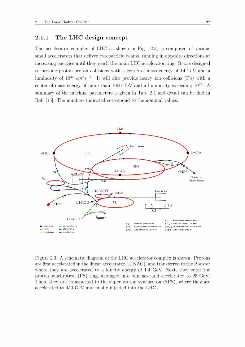
2.3 A schematic diagram of the LHC accelerator complex is shown. Pro-
tons are first accelerated in the linear accelerator (LINAC), and trans-
ferred to the Booster where they are accelerated to a kinetic energy of
1.4 GeV. Next, they enter the proton synchrotron (PS) ring, arranged
into bunches, and accelerated to 25 GeV. Then, they are transported
to the super proton synchroton (SPS), where they are accelerated to
450 GeV and finally injected into the LHC. . . . . . . . . . . . . . . . 27
2.4 An overview of the CMS detector. . . . . . . . . . . . . . . . . . . . . 33
2.5 The CMS detector’s transverse section. . . . . . . . . . . . . . . . . . 34
2.6 Hit coverage of the Silicon pixel detector. . . . . . . . . . . . . . . . . 36
2.7 Schematic cross section of the CMS silicon tracker. Each line corre-
sponds to a detector module while double lines correspond to back to
back modules. . . . . . . . . . . . . . . . . . . . . . . . . . . . . . . . 37
2.8 Layout of the CMS ECAL showing the arrangement of crystals, su-
permodules and endcaps with the preshower in front. . . . . . . . . . 38
2.9 A schematic cross sectional diagram of the ECAL, showing the ge-
ometrical arrangement of the barrel ECAL, the endcap ECAL, and
the preshower detector. The interaction point is located at the lower
left edge of the diagram. The dotted lines show the values of the
pseudorapidity at the given angle. . . . . . . . . . . . . . . . . . . . . 38
2.10 Longitudinal view of the CMS detector. The locations of the hadron
barrel (HB), the endcap (HE), the outer (HO) and the forward (HF)
calorimeters. . . . . . . . . . . . . . . . . . . . . . . . . . . . . . . . . 41
2.11 An r-z cross-section of a quadrant of the CMS detector with the axis
parallel to the beam (z) running horizontally and radius (r) increas-
ing upward. The interaction region is at the lower left corner. Shown
are the locations of the various muon stations and the steel disks (red
areas). The four drift tube (DT) stations are labeled MB (“muon bar-
rel”) and the cathode strip chambers (CSC) are labeled ME (“muon
endcap”). Resistive plate chambers (RPC, in green) are in both the
barrel and the endcaps of CMS. . . . . . . . . . . . . . . . . . . . . . 44
2.12 The individual drift tube cell and operation principle.. . . . . . . . . 45
2.13 Working principle of a CSC chamber. . . . . . . . . . . . . . . . . . . 46
2.14 A schematic diagram of the RPC double gap chamber. . . . . . . . . 47
2.15 Schematic representation of the CMS L1 trigger system. . . . . . . . 49
2.16 The structure of the CMS DAQ system. . . . . . . . . . . . . . . . . 51
2.17 Overview of CMS computing framework. . . . . . . . . . . . . . . . . 52

3.1 The basic structure of a showering and hadronization generator event
is shown schematically. . . . . . . . . . . . . . . . . . . . . . . . . . . 57
3.2 Cross-section for SM Higgs in H → 4`, H → 2e2mu and H → 4e (or
4µ) as a function of mH in pp collisions at√s = 7 (a). Cross-section
enhancement due to the interference of amplitudes with permutations
of identical leptons originating from different Z-bosons, as a function
of mH (b). . . . . . . . . . . . . . . . . . . . . . . . . . . . . . . . . 65
3.3 Electron identification efficiencies computed with the tag-and-probe
method as a function of the probe pT in two different η bins: (a) |η| <1.442 (barrel), (b) 1.556 < |η| < 2.5 (endcap). Results are for 8 TeV
data. . . . . . . . . . . . . . . . . . . . . . . . . . . . . . . . . . . . . 72
3.4 Muon reconstruction and identification efficiency for particle flow
muons, measured with the tag-and-probe method on 2012 data as
function of muon pT , in the barrel (left) and endcaps (right). . . . . . 76
3.5 Muon reconstruction and identification efficiency for Particle Flow
muons, measured with the tag-and-probe method on 2012 data as
function of the number of reconstructed primary vertices. . . . . . . . 78
3.6 Four lepton’s invariant mass distribution for significant background
processes in context of H→ ZZ∗ → 4` along with 3 Higgs signal samples. 82
3.7 The transverse momentum distribution of four lepton candidates for
relevant background processes in context of H→ ZZ∗ → 4` along with
3 Higgs signal samples. . . . . . . . . . . . . . . . . . . . . . . . . . . 82
3.8 Transverse momentum distributions of 4 highest pT leptons in an
event for mH = 125 GeV/c2 (a), mH = 200 GeV/c2 (b), mH = 350 GeV/c2
(c), WZ + jets (d), tt (e), Z + light jets (u, d, s) (f), Zbb (g) and Zcc
(h). . . . . . . . . . . . . . . . . . . . . . . . . . . . . . . . . . . . . . 83
4.1 Comparison of Z1 invariant mass in (a) ee 7 TeV, (b) µµ, 7 TeV (c) ee
8 TeV, (d) µµ, 8 TeV, between data and Monte Carlo expectations.
The samples correspond to data collected in 2011 (L = 5 fb−1 @ 7
TeV) and 2012 (L = 12.21 fb−1 @ 8 TeV) . . . . . . . . . . . . . . . 91
4.2 Event yields in the (a) 4e, (b) 4µ and (c) 2e2µ channels as a function
of the event selection steps. The MC yields are not corrected for
background expectation. The samples correspond to data collected
in 2011 L = 5.05 fb−1 @ 7 TeV. . . . . . . . . . . . . . . . . . . . . . 94
4.3 Event yields in the (a) 4e, (b) 4µ and (c) 2e2µ channels as a function
of the event selection steps. The MC yields are not corrected for
background expectation. The samples correspond to data collected
in 2012 L = 12.21 fb−1 @ 8 TeV. . . . . . . . . . . . . . . . . . . . . . 95
4.4 Probability density functions describing the NLO ZZ (left) and gg
→ ZZ (right) background shape for 4e (top), 4µ (middle), and 2e2µ
(bottom) final states. The distributions correspond to√s = 7 TeV. . 98
4.5 Fake rate measured for a probe lepton which satisfy loose selection,
in the Z(``) + e (left) and Z(``) +µ (right) samples as defined in the
text. The fake rates correspond to data collected in 2011(A+B) (a)
and (b), 2012 (A+B) (c) and (d), 2012 (C) (e) and (f). . . . . . . . . . 102
4.6 Fake rate measured for a probe lepton which satisfy loose selection,
in the Z(``) + e (left) and Z(``) + µ (right) samples as defined in
the text. The fake rates correspond to data collected in 2012 (A+B+C)
data taking periods. . . . . . . . . . . . . . . . . . . . . . . . . . . . . 103
4.7 DATA-MC comparison of the SS-SF (on the left) and OS-SF (on
the right) samples in the Z+X background control samples. (a) and
(b) represents 4e, (c) and (d) shows 4µ final states.The distributions
correspond to data collected in 2011 (L = 5 fb−1 @ 7 TeV). . . . . . . 107
4.8 DATA-MC comparison of the SS-SF (on the left) and OS-SF (on the
right) samples in the Z+X background control samples. (a) and (b)
represents 2e2µ, (c) and (d) shows 2µ2e final states. The distributions
correspond to data collected in 2011 (L = 5 fb−1 @ 7 TeV). . . . . . . 108
4.9 DATA-MC comparison of the SS-SF (on the left) and OS-SF (on the
right) samples in the Z+X background control samples. (a) and (b)
represents 4e, (c) and (d) shows 4µ final states. The distributions
correspond to data collected in 2012 (L = 12.21 fb−1 @ 8 TeV). . . . 109
4.10 DATA-MC comparison of the SS-SF (on the left) and OS-SF (on the
right) samples in the Z+X background control samples. (a) and (b)
represents 2e2µ, (c) and (d) shows 2µ2e final states. The distributions
correspond to data collected in 2012 (L = 12.21 fb−1 @ 8 TeV). . . . 110
4.11 (a) Invariant mass distribution of reconstructed Z boson (4µ) after
best Z1 selection (left) in accord with event selection methodology
of Ref. [69], whereas (b) shows the invariant mass distribution of
second reconstructed Z boson (4µ) as best Z2 after full event selection.
Shaded histogram displays MC samples and solid points represent
data corresponding to L = 4.71fb−1 @√s = 7 TeV. . . . . . . . . . 112

4.12 Distribution of reconstructed mass of Z1, Z2 and 4` in case of 4e (left)
and 4µ (right) final state. Shaded histogram displays MC samples and
solid points represent data corresponding to L = 4.71fb−1 @√s = 7
TeV. . . . . . . . . . . . . . . . . . . . . . . . . . . . . . . . . . . . . 115
4.13 Signal selection efficiencies for Higgs masses, 4e (a) and 4µ (b). Shaded
histogram displays MC samples and solid points represent data cor-
responding to L = 4.71fb−1 @√s = 7 TeV. . . . . . . . . . . . . . . 116
5.1 Distribution of the four-lepton reconstructed mass, (a) represents low
mass region and (b) is displaying full mass range considered in the
analysis. Region m4l < 100 GeV/c2 is shown but not used in analysis.
The sample correspond to an integrated luminosity of L = 5.1 fb−1
of 2011 data and L = 12.21 fb−1 of 2012 data. . . . . . . . . . . . . . 124
5.2 Fig. (a) and (b) are showing invariant mass distributions of Z1 and
Z2 respectively. The sample correspond to an integrated luminosity
of L = 5.1 fb−1 of 2011 data and L = 12.21 fb−1 of 2012 data. . . . . 124
5.3 Observed and expected 95% CL upper limit on the ratio of the pro-
duction cross section to the SM expectation with the 2D fit. 2011
and 2012 data-samples are used. The 68% and 95% ranges of expec-
tation for the background-only model are also shown with green and
yellow bands, respectively. (a) represents lower mass range only and
(b) shows full mass range. . . . . . . . . . . . . . . . . . . . . . . . . 125
5.4 Significance of the local fluctuations with respect to the standard
model expectation as a function of the Higgs boson mass for an inte-
grated luminosity of 5.1 fb−1 at 7 TeV and 12.21 fb−1 at 8 TeV in the
low mass range (110 - 180 GeV/c2) in (a) and in the mass range (110
-1000 GeV/c2) in (b). Dashed line shows mean expected significance
of the SM Higgs signal for a given mass hypothesis. . . . . . . . . . . 126


List of Tables
1.1 Fundamental interactions . . . . . . . . . . . . . . . . . . . . . . . . . 6
2.1 Design parameters of the Large Hadron Collider. . . . . . . . . . . . . 28
2.2 Contributions to the energy resolution of ECAL. . . . . . . . . . . . . 40
2.3 A summary of the main features of the CMS magnet. . . . . . . . . . 43
3.1 Datasets and trigger paths used in the analysis. CaloTrk
= CaloIdT CaloIsoVL TrkIdVL TrkIsoVL . . . . . . . . . . . . . . . 62
3.2 Trigger selections in 2012 data analysis. CaloTrk=CaloIdT CaloIsoVL TrkIdVL TrkIsoVL
and CaloTrkVT=CaloIdVT CaloIsoVT TrkIdT TrkIsoVT . . . . . . 63
3.3 Monte Carlo simulation datasets used for the signal and background
processes; Z stands for Z, Z∗, γ∗; ` means e, µ or τ ; V stands for W
and Z; pT is the transverse momentum for 2 → 2 hard processes in
the rest frame of the hard interaction. Comment: qq → ZZ∗ samples
at 8 TeV have lower cut in mll, 4 GeV instead of 12 GeV at 7 TeV.
TuneZ2 is used for 7 TeV, while TuneZ2star is used for 8 TeV analysis.
The low mass Drell-Yann was produced with a filter for the 8 TeV
analysis. . . . . . . . . . . . . . . . . . . . . . . . . . . . . . . . . . . 64
3.4 Filter efficiency for two different Drell-Yan samples. . . . . . . . . . . 80
4.1 Rate, purity and efficiency gain for signal and ZZ background. . . . 88
4.2 Definition of loose selection criteria for muon-like objects used for the
measurement of muon fake ratio. . . . . . . . . . . . . . . . . . . . . 99
4.3 Definition of loose selection criteria for electron-like objects used for
the measurement of electron fake ratio. . . . . . . . . . . . . . . . . 99
4.4 Muon Fake ratio’s over 2011(A+B) data . . . . . . . . . . . . . . . . . 103
4.5 Electron Fake ratio’s over 2011(A+B) data . . . . . . . . . . . . . . . . 104
4.6 Muon Fake ratio’s over 2012(A+B+C) data . . . . . . . . . . . . . . . . 104
4.7 Electron Fake ratio’s over 2012(A+B+C) data . . . . . . . . . . . . . . 104
4.8 (OSSS
)MC correction factor. . . . . . . . . . . . . . . . . . . . . . . . . 106
xi

4.9 The cut wise status of event yields of contributing samples in 4µ final
state . . . . . . . . . . . . . . . . . . . . . . . . . . . . . . . . . . . . 117
4.10 The cut wise status of event yields of contributing samples in 4e final
state . . . . . . . . . . . . . . . . . . . . . . . . . . . . . . . . . . . . 117
5.1 Number of ZZ background events expected and relative uncertainties
in the signal region estimated from Monte Carlo simulation, for 5.1
fb−1 at 7 TeV and 12.21 fb−1 at 8 TeV data. Uncertainty on the yields
due to QCD scale and the choice of parton distribution functions is
also reported. Only the Monte Carlo statistical uncertainty is shown. 119
5.2 The number of events from Z+X expected and the relative systematics
and statistical errors in the signal region in a mass range from m1 =
100 GeV/c2 to m2 = 600 GeV/c2. . . . . . . . . . . . . . . . . . . . . 121
5.3 The number of event candidates observed in 2011 data at L = 5.05 fb−1,
compared to the mean expected background and signal rates for each
final state for 100 < m4` < 1000 GeV/c2. For the Z + X background,
the estimations are based on data. . . . . . . . . . . . . . . . . . . . . 123
5.4 The number of event candidates observed in 2012 data at L = 12.21 fb−1,
compared to the mean expected background and signal rates for each
final state for 100 < m4` < 1000 GeV/c2. For the Z + X background,
the estimations are based on data. . . . . . . . . . . . . . . . . . . . . 123

Introduction
Physics is a scientific discipline and its primary aim is to describe all naturally oc-
curring phenomena in terms of the matter content of the universe and mutual inter-
action of matter, which results in inventions of numerous applications for mankind
from best available understanding of nature. Elementary particle physics addresses
these goals at the most fundamental level and attempts to comprehend the most
basic building blocks of matter to elucidate the basic interactions between them. In
the 20th century, a new experimental branch known as high energy physics (HEP)
evolves from this theoretical branch, which studies the interactions between elemen-
tary particles at very high energy. By using particle accelerators and colliders, these
high energy interactions allow the production of new particles which generally don’t
exist in nature under ordinary conditions.
Historically, progress in particle physics has followed a reductionist path, whereby
layers of complexity have been successfully explained in terms of ever more basic
building blocks. Atoms were reduced to electrons, protons and neutrons, and protons
and neutrons were in turn reduced to quarks and gluons. Similarly, the electric and
magnetic forces were combined into the electromagnetic force, which was in turn
combined with the weak force to give us the combined description of the electroweak
forces. These successes have converged, at the current state of our understanding,
to the theory of elementary particles and interactions known as the standard model
(SM) of particle physics. The SM predicts the existence of a unique physical Higgs
scalar boson associated to the spontaneous electroweak symmetry breaking, the so
called Higgs mechanism.
The SM is the quantum field theory (QFT), which has the greatest number of
experimental verifications till date. In particular, the Higgs boson mass, like those of
quarks, leptons and gauge bosons, is a free parameter of the theory. Direct searches
for the SM Higgs boson have been already performed at the e+e− collider LEP and
at the pp collider Tevatron. A lower bound of mH ≥ 114.4 GeV/c2 at 95% CL
(Confidence Level) has been set for the Higgs mass at LEP [1], while the D0 and
CDF experiments at Tevatron excluded the mass range 162 ≤ mH ≤ 166 GeV/c2
1

(95% CL) and reported an excess of events in the range 120-135 GeV/c2 [2]. Despite
the success of best available theoretical and experimental understanding of Particle
Physics, still we have some open fundamental questions as:
• What is the mechanism for electroweak gauge symmetry breaking, which gen-
erates the masses of the W and Z bosons ?
• What are the masses of the neutrinos and what is the mechanism that gener-
ates them [3] ?
• What is the origin of dark energy and dark matter, accounting for more than
95 % of the energy density of the universe and more than 80 % of its matter
[4] & [5] ?
The work presented in this thesis will contribute to get an answer of the first
question by using data collected with the CMS detector. The search for the SM
Higgs boson is one of the main goal of the CMS experiment at the Large Hadron
Collider (LHC) of CERN. The current analysis has been performed over proton-
proton collision data collected by the CMS detector in years 2011 (Lint = 5.05 fb−1
@√s = 7 TeV) and 2012 (Lint = 12.21 fb−1 @
√s = 8 TeV).
The searches for the SM Higgs boson has to cope with several SM or electroweak
processes that may have similar final states as those of the Higgs signal 1 and gen-
erally known as ‘background processes’. The development of accurate background
estimation techniques will lead to more confident experimental observation about
the existence or exclusion of the Higgs boson in that particular decay mode. An
experimental methodology has been developed to estimate all background processes
in a particular decay mode of the SM Higgs boson, when it decays as H → ZZ∗
and each Z boson further decays into a muon pair or electron pair.
In chapter 1, a short theoretical introduction to the SM Higgs physics and SM
background processes is given in context of H → ZZ∗ → 4` decay mode. The
production mechanism of relevant background processes and Higgs boson will be
briefly presented in the same. The chapter 2 contains a comprehensive description
of the LHC and CMS experiment. The reconstruction, identification and isolation
techniques for leptons are presented briefly in chapter 3. The key information about
Monte Carlo samples, event generators and data samples used in current analysis is
discussed in the same chapter.
1In accord with current work, the phase space populated by signatures of the SM Higgs boson-like events, is called ‘signal phase space’ and corresponding events are called ‘signal events’. Thesignal phase space is dedicated to examine the leptons coming from H→ ZZ∗ decay chain.
2

The studies about important physics observables over Monte Carlo simulations
are presented in the same, which helps to understand and finalize better working
points to differentiate between Higgs signal and background processes.
The chapter 4 will discuss background estimation methodologies in context of
H → ZZ∗ → 4` analysis. The principal sources of background come from almost
irreducible ZZ continuum, instrumental backgrounds such as Z+jets or WZ+jet(s)
where jets are misidentified as leptons and reducible background Zbb/Zcc, tt pro-
cesses, where Z and W’s undergoes leptonic decays and two secondary leptons pro-
duced within b-jets. Individual control regions (CR) are defined for the estimation
of corresponding backgrounds in Higgs signal phase space.
In addition, an alternate event selection methodology has been presented to
increase the event selection efficiency for Higgs signal.
The estimated values of contributing background processes along with relevant
sources of uncertainties are described in chapter 5. It also contains the complete
results about four lepton mass spectrum, the event yields of contributing signal and
background processes in signal phase space and statistical results of H → ZZ∗ →4` decay mode. The contribution of background estimation results in ZZ cross
section measurement and for H → ZZ∗ → 4` analysis by Bayesian approach will be
discussed briefly.
3

4

Chapter 1
The Standard Model
The fundamental components of matter and their interactions are described by the
standard model (SM) of particle physics, which is based upon two separate quantum
field theories (QFT) [6], describing the electroweak interaction (Glashow-Weinberg-
Salam model or GWS) and the strong interaction (Quantum Chromo-Dynamics or
QCD). Theoretical and experimental studies in particle physics for more than fifty
years have led to the development of the current SM of particle physics. Although it
is still incomplete, the SM is widely accepted as the most reliable theory to describe
all observed particles and their mutual interactions. In first half of current chapter,
a brief introduction to the theoretical base of the SM will be presented. For more
details, extensive bibliography is available in this subject as Ref. [7]. The production
mechanisms of the SM Higgs signal and relative background processes are discussed
briefly in second half of this chapter.
1.1 The Standard Model of Elementary Particles
The four fundamental forces that we observe in nature are the electro-magnetic
force, the weak force, the strong force and the gravitational force. The SM describes
all of these forces with the exception of the gravitational force because gravity is
extremely weak to have visible effects at the ‘TeV’ scale. In the SM, the interactions
between particles are described in terms of the exchange of bosons, integer-spin
particles which are carriers of the fundamental interactions. Each fundamental force
is associated with spin 1 mediator particles. The strong force is mediated by 8
colored gluons and the electromagnetic force is mediated by the photon, while the
weak interactions are mediated by the W± and Z bosons. The main characteristics
of fermions, bosons and corresponding interactions are summarized in Tab. (1.1)
and Fig. (1.1).
5

1.1. The Standard Model of Elementary Particles 6
Table 1.1: Fundamental interactions
Electromagnetic Weak Strong
Quantum Photon (γ) W±, Z GluonsMass (GeV
c2 ) 0 80, 90 0Coupling constant α(Q2 = 0) ≈ 1
137GF
(hc)3≈ 1.2 · 10−15(GeV
c2 ) α(mZ) ≈ 0.1
Range (cm) ∞ 10−16 10−13
Self-interaction No Yes Yes
The SM describes the matter as composed by twelve elementary particles, fermions
(6 quarks and 6 leptons) grouped in three generations. The higher generation par-
ticles decay via weak interactions to lower generation particles, explaining why the
low energy world (as it is known today) consists only of particles of the first gener-
ation. For each fermion, there exists also a corresponding anti-fermion which carry
same mass but opposite electric charge.
Figure 1.1: The SM fermions and bosons grouped in generations
The three leptons e−, µ−, τ− have charge of -1 while the corresponding neutrinos
are neutral. Neutrinos were introduced in the SM as massless particles however
recent results from neutrino oscillation experiments points that neutrinos having
1.2. The Higgs mechanism 7
very small but non- zero masses. Quarks are subject to both strong and electroweak
interactions and do not exist as free states, but only as constituents of a wide
class of particles, the hadrons, such as protons and neutrons. On the other hand,
leptons only interact through electromagnetic and weak forces. The three charged
leptons are identical with respect to interaction with all known fundamental forces
irrespective to their differences in mass.
The standard model is formulated mathematically as a field theory under the
SU(3) ⊗ SU(2)L ⊗ U(1) symmetry. SU(3) describes color and interactions
between gluons and quarks, while SU(2)L ⊗ U(1) describes electroweak interactions.
By Noethers theorem, each symmetry corresponds to a conservation law yielding
a conserved quantity, which, in the case of the standard model, are color, weak
isospin and hypercharge for the three symmetry groups mentioned respectively. In
the unbroken SU(2)L ⊗ U(1) symmetry, gauge bosons and fermions are required
to be massless. The mass of the weak bosons (W± & Z) is explained by breaking
of the symmetry between the electromagnetic and weak interactions via the Higgs
mechanism described in the next section.
1.2 The Higgs mechanism
The gauge bosons and fermions are massless by the electroweak unification theory
but experimentally it is not found true. This section describes spontaneous symme-
try breaking which is the mechanism through which weak gauge bosons are believed
to acquire their masses [6], [8]. To illustrate spontaneous symmetry breaking two
examples are studied, a global gauge symmetry and a local gauge symmetry applied
to U(1) and SU(2) symmetry groups. First we start from a complex scalar field
φ = (φ1 + iφ2)/√
2 described by the Lagrangian:
L = (∂µφ) ∗ (∂µφ)− µ2φ∗φ− λ(φ∗φ)2 (1.1)
where the first term is the kinetic energy term, the second term is the mass term
and the third term is an interaction term. This Lagrangian is invariant under global
gauge transformation φ → eiαφ with α independent on spatial coordinates. The
Lagrangian is
L =1
2(∂µφ1)2 +
1
2(∂µφ2)2 − 1
2µ2(φ2
1 + φ22)− 1
4λ(φ2
1 + φ22)2. (1.2)
If the case where λ > 0 and µ2 < 0 is considered, a circle of minima of the
potential V(φ) is observed in the φ1, φ2 plan of radius v, such that

1.2. The Higgs mechanism 8
φ21 + φ2
2 = v2 with v2 = −µ2
λ. (1.3)
The fact that the minimum is not at φ = 0 is very interesting for perturbation
theory to work; the Lagrangian has to be defined around the global minimum, that
is now at v. Therefore the field needs to be translated to the new minimum by
redefining it as:
φ(x) =
√1
2(v + η(x) + iξ(x)). (1.4)
Substituting the new field into the Lagrangian gives:
L′ = 1
2(∂µξ)
2 +1
2(∂µη)2 + µ2η2 +O(η3, ξ3, η4, ξ4). (1.5)
The third term shows that the new Lagrangian has acquired a new mass term for
the field η with mass µη =√−2µ2, however there is no term like that for the field
ξ. This is a consequence of the Goldstone theorem, which states that whenever a
continuos symmetry is spontaneously broken, always massless scalars occur in the
new theory (the field ξ in this case).
The next step is to repeat the same process in a local gauge invariant U(1) sym-
metry. So let’s assume a scalar field interacting with an electromagnetic field. The
theory is described by the Lagrangian:
L = |Dµφ|2 − µ2φ∗φ− λ(φ∗φ)2 − 1
4FµνF
µν (1.6)
where Dµ = ∂µ − ieAµ is the covariant derivative and the transformation is φ →eiα(x)φ. For µ2 < 0 the field has a new minimum v exactly as before. Translating
the Lagrangian to the new minimum gives:
L′ = 1
2(∂µξ)
2 +1
2(∂µη)2 + (−v2λη2) +
1
2e2v2AµA
µ
− evAµ∂µξ −1
4FµνF
µν + other interaction terms (1.7)
In this new Lagrangian, the field η has acquired a mass of mη =√
2λv2 but even
more important is the fact that the field Aµ has also acquired a mass mA = ev,
which implies that the gauge boson of this theory became massive. The residual
issue is that the field ξ is still massless, which implies that the Goldstone theorem
could still stand. In addition, the presence of a term Aµ∂µξ introduces a coupling
of the Aµ field to the scalar field. In terms of physics, the mass acquired by field
Aµ results as creation of one more polarization degrees of freedom i.e. longitudinal
1.2. The Higgs mechanism 9
polarization.
The additional term Aµ∂µξ provides the term needed to make the polarization
transverse because simply translating the field variables as in eq. 1.4, does not cre-
ate a new degree of freedom. Therefore the particle spectrum in the Lagrangian is
not correct and one of the fields in the Lagrangian doesn’t correspond to a particle.
The gauge invariance of the Lagrangian can be used to redefine it in a way that the
particle content is more understandable. The complex field was defined as:
φ =
√1
2(v + η + iξ) ≈
√1
2(v + η)e
iξv (1.8)
It implies that the gauge can be picked differently so that
φ→√
1
2(v + h(x))e
iθ(x)v (1.9)
Aµ → Aµ +1
ev∂µθ (1.10)
This particular choice of gauge transformation is known as the unitary gauge
and is designed to make h(x) real. Since θ appears as a phase factor, it will not
appear in the final Lagrangian. Substituting into eq. 1.6 gives the final Lagrangian
as:
L′′ = 1
2(∂µh)2 − λv2h2 +
1
2e2v2A2
µ − λvh3 − 1
4λh4
+1
2e2A2
µh2 + ve2A2
µh−1
4FµνF
µν (1.11)
In this new Lagrangian, the field Aµ has acquired a mass via the term 12e2v2A2
µ
and there is no massless Goldstone boson in the Lagrangian but a new scalar h with
a mass of m =√
2λv2 called the Higgs boson. So with this procedure the mass-
less Goldstone boson has been converted to the additional longitudinal polarization
degree of freedom so that the field acquires mass resulting in a Lagrangian with
a scalar massive particle, a massive field and interaction terms. This procedure is
known as the Higgs mechanism. For this mechanism to be the way for vector bosons
to acquire mass in nature, a new particle must exist. The Higgs boson has not
been yet discovered and the purpose of this thesis is to contribute in this quest by
estimating the background processes of H → ZZ∗ → 4` decay channel.

1.2. The Higgs mechanism 10
The last step is to apply the Higgs mechanism to the electroweak model based
on SU(2)L ⊗ U(1)Y symmetry and create mass for the vector bosons and fermions.
We use the covariant derivative:
Dµ = ∂µ + igTaWaµ + i
g′
2BµY, (1.12)
which corresponds to gauge invariance for the SU(2)L ⊗ U(1)Y symmetry. Substi-
tution of eq. 1.12 in the Lagrangian of the scalar field (i.e. eq. 1.1 ) gives:
L =
∣∣∣∣(i∂µ − gTa ·W aµ − g′Bµ
Y
2
)φ
∣∣∣∣2 − V (φ) (1.13)
For this Lagrangian to be invariant, φ must be invariant under SU(2)L ⊗U(1)Y
symmetry. A choice satisfying this is using an isospin doublet with Y=1:
φ =
(φ+
φ0
)(1.14)
whereφ+ ≡ (φ1 + iφ2)/
√2
φ0 ≡ (φ3 + iφ4)/√
2
The new field will have a vacuum expectation value of
φ0 ≡1√2
(0
v
)(1.15)
Expanding the kinetic term of the scalar field and using the Pauli matrices as
the generators of SU(2) gives:∣∣∣∣(−igTa2 W aµ − i
g′
2Bµ
)φ
∣∣∣∣2 =
1
8
∣∣∣∣∣(
gW 2µ + g′Bµ g(W 1
µ − iW 2µ)
g(W 1µ + iW 2
µ) −gW 3µ + g′Bµ
)(0
v
)∣∣∣∣∣2
=
(1
2vg
)2
W+µ W
−µ +v2
8(W 3
µ , Bµ)
(g2 −gg′
−gg′ g′2
)(W 3µ
Bµ
)
where we used theW raising and lowering operators, defined asW±µ =
(W 1µ ∓ iW 2
µ
)/√
2.
The first term in this expression corresponds to a massive W boson with mass of

1.2. The Higgs mechanism 11
MW = vg/2. The matrix term can be expressed as a function of the fields A and Z
by finding a transformation between W 3, B and A,Z that diagonalizes the matrix
so that the elements in the diagonal are the mass terms 12M2
ZZ2µ,
12M2
AA2µ, for Z and
A respectively. The transformation is:
Aµ =g′W 3
µ + gBµ√g2 + g′2
(1.16)
Zµ =gW 3
µ − g′Bµ√g2 + g′2
(1.17)
from which is derived that MA = 0 (the photon remains massless) and MZ =v2
√g2 + g′2. Therefore all gauge bosons gained mass, the photon mass is zero and
there is one additional scalar particle. The two couplings g and g′ are related by
electroweak unification via the weak mixing angle θw as tanθw = g′/g. The final step
is to give mass to the fermions. The problem in SU(2)L⊗U(1)Y was that the mass
term mψψ was not invariant. This can be solved by introducing a fermion coupling
to the Higgs. In case of electrons, a term can be added in the Lagrangian of the form:
Le = −K
[(νe e−)
L
(φ+
φ
)eR + e−R (φ− φ0)
(νe
e
)L
](1.18)
Substituting the form of the Higgs field in the unitary gauge the Lagrangian
becomes
Le = − K√2v(e−LeR + e−ReL)− K√
2v(e−LeR + e−ReL)h (1.19)
Picking the constant K such as that me = Kv/√
2 gives a fermion mass term in the
Lagrangian:
Le = −mee−e− me
ve−eh, (1.20)
Therefore the electron has acquired mass and a new coupling has been introduced
between the Higgs boson and the fermions proportional to the ratio of the electron
and W mass, which is very small since me is small.

1.3. Z and Higgs Boson Production in p-p collisions 12
1.3 Z and Higgs Boson Production in p-p colli-
sions
The standard model describes all interactions between quarks and leptons. Those
interactions result in production and decay of the W±, Z and Higgs bosons. However
to study scalar and vector boson production in proton collisions, the hard interaction
between quarks and gluons has to be separated from the proton substructure. The
quarks inside the proton are not free but are strongly bound, exchanging colored
gluons. The continuous interactions between the quarks makes them virtual particles
lying off their mass shell. Gluons are carrying about 50% of the proton momentum
and can produce additional quark-antiquark pairs (e.g. bb). The quark content of
the proton is separated into the valence quarks (u, d), the sea quarks (u, d, s, c) and
the gluons, together called partons.
Therefore, in a proton collision, any quark or gluon combination can contribute
to the hard scattering process. The probabilities for a specific parton with a given
momentum fraction of the proton to participate in the hard process are known as
parton distribution functions and measured by using data from deep inelastic scat-
tering experiments. Therefore the center of mass energy√s for each hard scattering
process is related to the center of mass energy of the two colliding protons√S as:
s = xyS (1.21)
where x, y are the momentum fractions of the contributing partons. One im-
portant aspect of hadron colliders is that those parton distribution functions make
them versatile machines for discovery although the hard scattering center of mass
is not well defined. If the center of mass energy of the protons is high enough, de-
pending on the parton momentum fractions, every collision will create particles of
different masses and the possibility to observe new physics increases. This section
describes the phenomenology of Z, a rare decay process of Z→ 4` and Higgs bosons
production mechanism in proton collisions.
1.3.1 Z boson production
The Z boson is produced in proton-proton collisions at leading order by fusion of
quark- antiquark pairs. The simplest diagram that can create a Z boson is shown
in Fig 1.2 (a). In this process, the Z boson has no transverse momentum but is
created and moving along the beamline. This process can create a virtual photon

1.3. Z and Higgs Boson Production in p-p collisions 13
that will decay to a fermion pair or a Z boson or a W+W− boson or ZZ. Neglecting
the virtual photon part and assuming massless fermions, the matrix element for the
Z production is:
Figure 1.2: Z boson production mechanisms in hadron colliders.
|M|2 = (s√
2gZ)2 (gV )2 + (gA)2
2M2
Z = 32GF√
2(g2V + g2
A)M4Z (1.22)
and the differential cross section at parton level is:
σ = 8πGF√
2(g2V + g2
A)M4Zδ(s−M2
Z), (1.23)
where s is the center of mass energy of the colliding quarks. This formula implies
that to create a Z boson, the two quarks must have a center of mass energy equal to
the mass of Z boson. In lepton colliders where elementary particles are colliding, the
energy of the beams is set to the Z mass to create a Z boson. In hadron colliders the
situation is different. In the LHC, protons are colliding at a large constant energy of√s = 7 TeV in 2011 and
√s = 8 TeV in 2012. For the Z to be created, two partons
from the proton should interact. Those partons must be a quark-antiquark with
suitable momentum fractions x, y such that s = xyS. Then the parton distribution
functions are integrated for x, y to give the full cross section:

1.3. Z and Higgs Boson Production in p-p collisions 14
σ =8π
3
GF√2
∫dxdy
∑(g2V + g2
A)xySfq(x)fq(y) (1.24)
where the integration is performed under the constraint xyS = M2Z and fq are
the parton distribution functions (PDF). The sum runs over all quarks.
There is a significant contribution from higher order diagrams such as one shown
in Fig 1.2 (b) resulting in an additional parton in the final state that hadronizes
to a jet. Those types of events are also observed and constitute very important
background in Higgs searches as it is described in next sections.
In terms of the Z decay signature, the Z boson decays primarily to hadrons or
lepton pairs according to the V −A couplings. Z decays to a pair of leptons about
3% of the time for each lepton flavor and the most straightforward final state for Z
measurement is a muon or electron pair.
1.3.2 Z → 4` process
This process is referred as single-resonant four-lepton production. The leading order
(LO) Feynman diagram for the production and decay of qq → Z → 4` is displayed
in Fig. 1.3. It has been shown in Ref. [9] that the Z → 4` decay gives a clean
resonant peak in the four-lepton invariant mass distribution and number of events
in the Z → 4` peak at m4` = mZ is an order of magnitude larger than the expected
number of events for the SM Higgs boson with a mass mH anywhere in the remaining
allowed range of 117.5 - 118.5 GeV/c2 and 122.5 - 127.5 GeV/c2 (see Ref. [10, 11]).
Figure 1.3: The qq → Z → 4` decay process.

1.3. Z and Higgs Boson Production in p-p collisions 15
Therefore, the Z→ 4` peak can be used for a direct validation for understanding
the four-lepton mass scale and the four-lepton mass resolution in the phase space to
the Higgs boson four-lepton decays.
1.3.3 Higgs boson production
The main processes contributing to the Higgs boson production at a proton-proton
collider are represented by the Feynman diagrams in Fig. 1.4. The corresponding
cross sections are shown in Fig. 1.5 for centre-of-mass energies of 7 TeV and 8 TeV
[12]. The 7 TeV is the energy provided by the LHC during the 2010 - 2011 runs and
8 TeV energy corresponds to runs collected in 2011 - 2012. The total production
cross section at 7 TeV is lower than at 8 TeV as shown in Fig. 1.5.
The Higgs boson couples with a strength proportional to the mass, therefore, it
has large couplings to W and Z boson pairs. In terms of the fermions, the introduced
Yukawa couplings impose a dependence of the coupling as m2f , therefore the Higgs
coupling is enhanced for heavy quarks (especially t) and leptons (especially τ). The
dominant production modes of Higgs boson are discussed below:
1.3.3.1 Gluon-Gluon Fusion
The gluon fusion [12] through a heavy quark loop is the dominating mechanism for
the Higgs boson production at the LHC over the entire mass range 1 due to high
luminosity of gluons. The process is shown in Fig. 1.4 (a) with a t quark-loop, which
is the main contribution due to its large Yukawa coupling to the Higgs boson. The
dynamics of the gluon-fusion mechanism is controlled by strong interactions, which
require detailed studies of the effect of QCD radiative corrections and evaluation of
electroweak (EW) corrections to obtain accurate theoretical predictions.
The latest results in the computation of the cross section for this process are
shown in Fig. 1.5 and used in the analysis presented in this thesis, include next-
to-next-to-leading order (NNLO) QCD contributions, complemented with next-to-
next-to-leading log (NNLL) re-summation, and next-to-leading order (NLO) elec-
troweak corrections.
An uncertainty of 15-20% on the calculation of this partonic cross section is
assumed, mostly depending on the choice of the parton density functions (PDFs),
implementation of the EW corrections, missing terms in the perturbative expansion
and on the uncalculated higher-order QCD radiative corrections.
1100 GeV/c2 ≤MH ≤ 1 TeV/c2 being investigated at LHC.

1.3. Z and Higgs Boson Production in p-p collisions 16
(a) (b)
(c) (d)
Figure 1.4: Higgs boson production mechanisms at tree level in proton-proton col-lisions: (a) gluon-gluon fusion, (b) vector boson fusion, (c) W and Z associatedproduction (or Higgsstrahlung), and (d) tt associated production.
(a) (b)
Figure 1.5: Cross sections for the different Higgs boson production modes, as func-tions of the Higgs boson mass, at LHC’s centre-of-mass energy equal to 7 TeV (a)and 8 TeV (b) (see Ref. [12]).

1.3. Z and Higgs Boson Production in p-p collisions 17
1.3.3.2 Vector Boson Fusion (VBF)
The production of the standard model Higgs boson via fusion of a pair of W or Z
bosons in association with two hard jets in the forward and backward regions of
the detector, frequently quoted as the vector-boson fusion (VBF) channel [12] and
shown in Fig. 1.4 (b). It is second most dominant production mechanism of the
Higgs-boson at the LHC. Higgs-boson production in the VBF channel plays also an
important role in the determination of Higgs-boson couplings at the LHC. Bounds on
non-standard couplings between Higgs and electroweak (EW) gauge bosons can be
imposed from precision studies in this channel. In addition this channel contributes
in a significant way to the inclusive Higgs production over the full Higgs-mass range.
The production of a Higgs boson + 2 jets receives two contributions at hadron
colliders. The first type, where the Higgs boson couples to a weak boson that links
two quark lines, is dominated by t- and u-channel-like diagrams and represents the
genuine VBF channel. The hard jet pairs have a strong tendency to be forward-
backward directed in contrast to other jet-production mechanisms, offering a good
background suppression (transverse-momentum and rapidity cuts on jets, jet rapid-
ity gap, central-jet veto etc.).
The presence of two spectator jets with high invariant mass in the forward region
provides a powerful tool to tag the signal events and discriminate the backgrounds,
thus improving the signal to background ratio, despite the low cross section. More-
over, both leading order and next-to-leading order cross sections for this process
are known with small uncertainties and the higher order QCD corrections are quite
small. It is about one order of magnitude lower than gg fusion for a large range
of mH values and the two processes become comparable only for very high Higgs
masses (O(1 TeV)).
1.3.3.3 Associated Production
The production of the SM Higgs boson in association with a W± and Z bosons is
usually defined as Higgsstrahlung processes, which can be used to tag the event.
The process is shown in Fig. 1.4 (c) and is several orders of magnitude lower than
those of gg-fusion and VBF. It have been considered mainly by exploiting two decay
modes, H → W+W− and H → bb. The former is examined as it could contribute
to the measurement of the Higgs boson coupling to W bosons and the latter decay
mode might contribute to the discovery of a low-mass Higgs boson and allow to
measure the coupling of the Higgs boson to b quarks. The cross section for this
process is known at the NNLO QCD and NLO EW level. The inclusion of these
available contributions increases the LO cross section by about 20-25%.

1.3. Z and Higgs Boson Production in p-p collisions 18
The last process, illustrated in Fig. 1.4 (d), is the associated production of a
Higgs boson with a tt pair. Also for this process, the cross section is orders of
magnitude lower than those of gluon and vector boson fusion. The presence of the
tt pair in the final state can provide a good experimental signature. For this cross
section, NLO QCD calculations are available.
1.3.3.4 Decay modes of the SM Higgs boson
The SM Higgs boson decays primarily to fermion or boson pairs and the branching
ratio is enhanced for heavier particles. The Higgs boson decay branching fractions
as a function of the Higgs mass are presented in Fig. 1.6.
For low Higgs mass, the primary decays are via bb and ττ while for higher masses
the WW and ZZ final states dominate. For mH ≈ 2mt, the Higgs decay to top pairs
also contributes. Despite the structure of the couplings, the most sensitive modes
for the Higgs boson depends upon the experimental reasons. For example, at low
mass, the bb final state can only contribute via associated production (WH,ZH)
since the pp→ bb background is overwhelming.
Figure 1.6: The SM Higgs boson decay branching fractions as a function of the Higgsmass.

1.4. The SM Background Processes 19
In the same sense, H → ττ dominantly contributes via V BF topologies due to
the overwhelming Z → ττ background from other production mechanisms. On the
other hand, ZZ and WW decay modes also contribute to lower mass Higgs searches
because of the clean experimental signatures as leptonic decays i.e. ZZ → 4` and
WW → 2l2ν. Finally H → γγ has very low branching ratio but the relatively clean
two photon signature provides the best sensitivity at low mass.
1.4 The SM Background Processes
The background processes are described in context of H→ ZZ∗ → 4` decay mode.
Here and henceforward, Z stands for Z,Z∗ and γ∗ (wherever applicable). For the
event generation, ` is to be understood as being any charged lepton, e, µ or τ . The
predominant source of backgrounds giving 4 leptons as final state are:
• irreducible ZZ continuum, which gives 4 lepton in final state as qq→ ZZ∗ → 4`
and gg→ ZZ∗ → 4`.
• reducible backgrounds as Zbb, Zcc & tt processes.
• instrumental backgrounds such as Z+jets or WZ+jet(s).
The analysis will focus on reconstructed final states with electrons or muons only
and considered final states are: 4µ, 4e, 2µ2e. The production mechanism of some
of the main backgrounds is discussed briefly in following sections.
1.4.1 Irreducible backgrounds
The four-lepton events from non resonant di-boson production constitute the
main source of background events. This background is called ‘ZZ continuum’ for
simplicity throughout the succeeding sections and will be considered in the category
of irreducible backgrounds, as the event topology and kinematics is very similar to
those of Higgs signal events.
The lowest order production mechanism is the one represented in Fig. 1.7a as
qq → ZZ∗/Zγ∗. In case of SM Higgs boson production via the gluon fusion mech-
anism, the gluon-induced ZZ background, although technically of NNLO compared
to the first order Z-pair production, amounts to a non-negligible fraction of the total
irreducible background at masses above the 2mZ threshold. The associated diagram
gg → ZZ∗/Zγ∗ is represented in Fig. 1.7b.

1.4. The SM Background Processes 20
(a)
(b)
Figure 1.7: Lowest order diagrams for the qq → ZZ∗/Zγ∗ process (a) and for thegg → ZZ∗/Zγ∗ process (b).
1.4.2 Reducible backgrounds
The instrumental & reducible backgrounds are contributing in 4 lepton signal
phase space because jets can be misidentified as leptons, Z & W’s undergoes leptonic
decays and b-jets can produce other two leptons from secondary vertices. In addi-
tion, the multiple jet production from QCD hard interactions can also contribute
in early stages of the analysis, as well as other di-boson (WW,WZ,Zγ) and single
top backgrounds.
In the category of reducible backgrounds, those with final state leptons coming
from b (c) decays are the most important. The main source of background events
of this type are the associated production of Zbb/Zcc with Z → `+`− decays, as
shown in Fig 1.8. In addition, the production of top quark pairs in the decay
mode tt→ W+bW−b→ `+`−ννbb have a considerable contribution among reducible
backgrounds and shown in Fig 1.9. The B mesons can decay semi-leptonicaly in three
different ways:
• with a direct decay (b→ `, BR ≈ 10.7%),
• with a cascade decay (b→c→ `, BR ≈ 8%),
• with a ‘wrong sign’ cascade decay (b→c→ `, BR ≈ 1.6%).

1.4. The SM Background Processes 21
So these processes with two b/c quarks decaying leptonicaly can lead to 4` final
state events. These backgrounds are called reducible as the experimental signature
of leptons from b/c decay can be separated from that of leptons from W and Z
decays because those are prompt leptons, which gives different kinematical behavior
of final decay products.
(a) (b)
Figure 1.8: Some of the probable decay modes for Zcc (a) and Zbb (b), which cangive 2` + 2 heavy flavor jets.
Figure 1.9: One of the expected decay mode of tt.

1.4. The SM Background Processes 22
1.4.3 Instrumental backgrounds
The category of instrumental backgrounds is used to indicate background events
with final state leptons from mis-identification of other particles like jets, e.g. Z
+ light flavor jets (u,d,s), QCD multi-jets and WZ + jets processes where leptons
mainly comes from jets faking leptons.
In WZ + jets, the jets can originate from the hadronisation of both light (u, d,
s) and heavy (c, b) quarks. Fig 1.10a represents WZ + jets→ `±ν`′+`
′−(`, `′= e, µ
where one jet in final state can be mis-identified as lepton. Similarly in case of
Z + jets decays (see Fig 1.10b, 1.11a & 1.11b) as 2` + 2 light jets where these 2
additional jets can fake leptons.
(a)
(b)
Figure 1.10: One of the probable decay modes for WZ+jet(s) decaying to 3` + 1 jet+ 1 ν final state (a) and Z+uu (b).

1.4. The SM Background Processes 23
More precisely this is the general case for electrons, while reconstructed muons
in these processes, in addition to those from the Z and W decay, mainly comes from
decay in fight of light primary hadrons.
(a)
(b)
Figure 1.11: Probable decay modes for Z+dd (a) and Z+ss (b).

1.4. The SM Background Processes 24
Chapter 2
Experimental Apparatus
The Large Hadron Collider, LHC [13, 14] has been built by using the existing LEP
tunnel at CERN under French and Swiss territory, to carry on research in fundamen-
tal physics. This machine is an excellent scientific and technical milestone towards
understanding nature and the SM Higgs physics. It is the largest circular collider
and the highest energy particle accelerator ever built because a large amount of
energy is required in order to produce heavier fermions, which can couple stronger
with the Higgs boson or can boost its production.
2.1 The Large Hadron Collider
The design of the LHC started in 1981, but the project was not approved by CERN
council until December 1994. The building and commissioning of the LHC was a
huge technological effort. The magnitude of the experiment, the biggest ever built,
caused some unpredictable delays and during fifteen years the design has consid-
erably evolved and matured but the original idea stayed untouched. In the years
to come, LHC will reach its design energy and luminosity, and particle physics will
enter new territories that have never been explored before by previous colliders. The
total integrated luminosity delivered by LHC in different time spans since beginning
is shown in Fig. 2.1 & 2.2.
The LHC started providing pp collisions on 23 November 2009, at the centre-of-
mass energy of√s = 900 GeV. This energy was then raised to
√s = 2360 GeV and
later, on 30 March 2010, the first collisions at a centre-of-mass energy of 7 TeV, the
highest ever reached at a particle collider, were recorded by the four experiments
[15]: ALICE, ATLAS, CMS and LHCb.
25

2.1. The Large Hadron Collider 26
Figure 2.1: Integrated luminosity versus time delivered to, and recorded by CMS(see Sec. 2.2) during stable beams for pp running at 8 TeV centre-of-mass energy.
Figure 2.2: Total integrated luminosity vs. time since the startup of the LHC.
2.1. The Large Hadron Collider 27
2.1.1 The LHC design concept
The accelerator complex of LHC as shown in Fig. 2.3, is composed of various
small accelerators that deliver two particle beams, running in opposite directions at
increasing energies until they reach the main LHC accelerator ring. It was designed
to provide proton-proton collisions with a center-of-mass energy of 14 TeV and a
luminosity of 1034 cm2s−1. It will also provide heavy ion collisions (Pb) with a
center-of-mass energy of more than 1000 TeV and a luminosity exceeding 1027. A
summary of the machine parameters is given in Tab. 2.1 and detail can be find in
Ref. [15]. The numbers indicated correspond to the nominal values.
Figure 2.3: A schematic diagram of the LHC accelerator complex is shown. Protonsare first accelerated in the linear accelerator (LINAC), and transferred to the Boosterwhere they are accelerated to a kinetic energy of 1.4 GeV. Next, they enter theproton synchrotron (PS) ring, arranged into bunches, and accelerated to 25 GeV.Then, they are transported to the super proton synchroton (SPS), where they areaccelerated to 450 GeV and finally injected into the LHC.

2.1. The Large Hadron Collider 28
Table 2.1: Design parameters of the Large Hadron Collider.
Large Hadron Collider
circumference 26659 mdepth 50 - 175 m
total number of magnets 9600number of main dipoles 1232number of quadrupoles 392
temperature 1.9 K (-271.3 C)beam vacuum pressure 10−13atm
nominal p energy 7 TeVcenter-of-mass energy 14 TeV
design luminosity 1034 cm2s−1
bunches per proton beam 2808protons per bunch 1.1 ×10¹¹
turns per second 11245collisions per second 600 milionslength of each dipole 15 mweight of each dipole ≈ 35 t
dipole field 8.33 T
2.1.1.1 LHC Collision Detectors
The detectors are installed in the collision points all around the LHC ring. There are
six experiments installed at the LHC, in alphabetical order: ALICE (A Large Ion
Collider Experiment), ATLAS (A Toroidal LHC Apparatus), CMS (Compact Muon
Solenoid), LHCb (Large Hadron Collider beauty), LHCf (Large Hadron Collider
forward) and TOTEM (TOTal Elastic and diffractive cross-section Measurement).
ALICE, ATLAS, CMS and LHCb are installed in four huge underground caverns
build around the four collision points of the LHC, while LHCf and TOTEM are close
to the main detectors, ATLAS and CMS respectively. ATLAS and CMS are the main
experiments in the LHC, made for general purposes with the same physics goals but
different technical solutions and design; the rest of the experiments are smaller and
specialized in different topics.
This thesis have been realized in context of the CMS experiment. The main
details about the CMS detector will be discussed in the following sections.

2.1. The Large Hadron Collider 29
2.1.2 Performance Goals and Constraints
The LHC is designed to reach a center of mass energy up to 14 TeV. For any physics
process the number of events generated by the LHC collisions is given by:
Nevent = Lσevent (2.1)
where L is the instantaneous machine luminosity and σevent is the production
cross section for this specific physics process. The machine luminosity depends on
the beam parameters and for a Gaussian distributed beam is given by:
L = FN2b nbfrevγr4πεnβ∗
(2.2)
where F is the geometric luminosity reduction factor due to the crossing angle
at the interaction point (IP), Nb is the number of particles per bunch, nb is the
number of bunches per beam, frev represents the revolution frequency, γr is rela-
tivistic gamma factor, εn the normalized transverse beam emittance and β∗ is the
beta function at the collision point. The beam emittance and the β∗ are determined
from the single particle transverse motion described by the equation:
x(s) = A√β(s)cos[ψ(s) + δ] (2.3)
where s is the path along beam direction and A, δ are constants of integration
defined by boundary conditions. The amplitude function, β, describes the amplitude
of the motion in the beam line. The phase depends on β and advances as dψ/ds =
1/β. The amplitude function at the IPs, where magnets are configured to focus the
beams is designated as β∗. The number of transverse oscillations per rotation is
denoted as the tune (ν). The phase space of the motion in the transverse plane is
described by an ellipse in the (x, x′) plane where x′ = dx/ds. This ellipse has a
total area of πA2. If we consider a particle ensemble populating the phase space, we
define as emittance the area populated by this particle ensemble. This area depends
only on the beam energy. For a Gaussian one dimensional beam, the emittance is
defined as :
ε = πσ2
β(2.4)
The geometric luminosity reduction factor is given by:
F =
(1 +
(θcσz2σ∗
)2)−1/2
(2.5)

2.1. The Large Hadron Collider 30
where θc is the full crossing angle in the IP, σz is the RMS bunch length and σ∗ the
transverse RMS beam size at the IP. The LHC is designed to operate at a maximum
luminosity of the order of L = 1034cm−2s−1. That implies nominal operation with
large number of bunches (2,808 per beam) and bunch crossings spaced by 25 ns. To
reach this luminosity, very large proton density is required. Therefore, proton-proton
beams are used providing the highest beam currents.
The limitations to the maximum instantaneous luminosity come from several fac-
tors. The particle density per bunch is mainly limited by the non-linear beam-beam
interactions between particles when beams collide with each other. Beam-beam in-
teractions result in modification of the tune of the particles. which is expressed via
the linear tune shift given by:
ξ =Nbrp4πεn
. (2.6)
In this equation, rp is the classical radius of the proton (rp = e2/4πε0mpc2). The
linear tune shift should not exceed 0.015 when summed over all IPs in the machine.
Another parameter that affects luminosity is the mechanical aperture which is given
by the beam screen dimensions. The beam screen in the LHC has a width of 2 ×22 mm and a height of 2 ×17.3 mm. Setting the aperture at 10σ in terms of the
RMS beam size and accounting for imperfections in design and alignment results in
a maximum nominal beam size of 1.2 mm. Combined with a maximum β-function of
180 m in the arcs, this implies a maximum emitance of ε = 3.75 µm. This parameter
in combination with the linear beam-beam tune shift, limits the particle density to
Nb = 1.15× 10¹¹.
Furthermore, the mechanical aperture limits the β∗ value at the IPs resulting
in lower peak luminosity. Other design parameters that affect the peak luminosity
are related to the maximum dipole field, the maximum energy that can be stored
in the machine, the heat load, the quality of the magnetic field and the beam in-
stabilities due to electromagnetic interactions between particles and the conducting
boundaries of the vacuum. The dipole field corresponding to a beam energy of 7
TeV is 8.33 T. However, the operating dipole field depends on the heat load and
temperature margins inside the cryo-magnets and therefore on beam losses, causing
high dipole field to require very low beam losses during operation. Heat load refers
to heat deposition that is absorbed by the cryogenic system and it is usually due to
energy losses and synchrotron radiation. Synchrotron radiation is given by Larmors
formula:
P =1
6πε0
e2α2
c3γ4. (2.7)

2.2. The CMS detector 31
where α is the centripetal acceleration. Although the LHC is a proton collider,
7 kW have to be removed at 1.8K around the ring due to heating from synchrotron
radiation which is an experimental challenge for the LHC.
Other parameters that limit the peak luminosity are related to the operation of
the machine. The most important metric for LHC Physics program is the integrated
luminosity for a run which is defined as:
Lint = L0τL[1− e−Trun/τL ] (2.8)
where L0 is the initial instantaneous luminosity, τL is the net luminosity lifetime
and Trun is the total length of the luminosity run. The luminosity lifetime depends
on collisions that can degrade the beam and other effects like beam-beam interac-
tions, radiation and scattering of particles in the residual gas. The average design
luminosity lifetime for LHC is
τL = 14.9 h (2.9)
The LHC is designed for long term operation. It will operate for about 200
days per year. One significant parameter for high integrated luminosity is the turn-
around time, which is the time from the end of the run to the beginning of a new one.
Ideally this time is about 1.15 hr due to magnet hysteresis, however experience in
the operation of LHC and other accelerators has shown that a more realistic value is
of the order of 7 hr. All those parameters limit the maximum integrated luminosity
that the LHC provides in design conditions to 80 to 120 fb−1 per year.
2.2 The CMS detector
The CMS detector has been built to reconstruct precisely the final states including
muons, electrons, photons and jets, which will lead towards detection or exclusion of
the SM Higgs boson and discovery of new physics. Neutrinos and other very weakly
interacting particles escape without leaving signals, they can only be measured in-
directly through the determination of missing transverse energy, which requires a
hermetic detector. Therefore CMS must cover the solid angle as much as possible.
For this purpose, new forward detectors have been added to the original CMS design.
The structure of the CMS detector is sketched in Fig. 2.4. Two endcaps close a
cylindrical barrel part. The overall diameter is 14.6 m, the length 21.6 m, the weight
about 12500 tons. The thickness of the electromagnetic calorimeter, expressed in
radiation lengths, is larger than 25 X0, while the one of the hadronic calorimeter,

2.2. The CMS detector 32
expressed in interaction lengths1, ranges from 7 to 11 λ1 depending on η.
The CMS cartesian coordinate system is a right-handed reference frame with
the x-axis pointing towards the centre of the LHC ring, the y-axis pointing up-
wards and the z-axis parallel to the beam. The origin is located at the nominal
interaction point. In this reference frame, let the quadri-momentum of a particle
be (E, px, py, pz). The longitudinal momentum is pz, the transverse momentum is
pT =√p2x + p2
y. The rapidity is defined as:
y =1
2· ln(E + pzE − pz
)(2.10)
If a particle is ultra-relativistic (p � m), its rapidity can be approximated by
the pseudo srapidity η, defined as:
η = −ln(tan
θ
2
)(2.11)
θ being the angle between the +z semi-axis and the particle momentum vector
~p.
From the interaction point outwards, the CMS layout can be described as an
‘onion-like’ sequence of subdetectors as shown in Fig. 2.4. The innermost one is the
Inner Tracking System (see Sec. 2.2.1), made up of a silicon pixel vertex detector
and of a silicon strip tracker. The former has 3 layers in the barrel and 2 disks
in each endcap, the latter consists of 10 layers in the barrel region and 12 disks
in the endcaps. The main goal of the tracker is the precise reconstruction of the
position of primary and secondary vertices and the accurate measurement of the
impact parameter of charged tracks. This is possible even in the case of a high track
multiplicity, because of the very fine segmentation of the sensors.
The electromagnetic calorimeter (ECAL) (see Sec. 2.2.2) is located outside of the
tracker volume. It is a homogeneous detector consisting of lead tungstate (PbWO4)
scintillating crystals that are read out by avalanche photo diodes or vacuum pho-
totriodes. Its aim is the precise measurement of the energy and position of electrons
and photons. The pseudo-rapidity coverage reaches |η| < 3.0. In the endcap re-
gion, a lead/silicon pre-shower detector is installed in front of ECAL in order to
improve the resolution of electron and photon direction measurements and to help
discriminate between photons and neutral pions. The hadronic calorimeter (HCAL)
1Nuclear interaction length is defined as the mean path length in which the energy of relativisticcharged hadrons is reduced by the factor of 1/e as they pass through matter.

2.2. The CMS detector 33
Figure 2.4: An overview of the CMS detector.
(see Sec. 2.2.3) surrounds ECAL. It is a sampling calorimeter consisting of brass
absorber plates interspersed with scintillator layers. It is designed to reconstruct
energy and position of hadrons and jets. The barrel (HB) and endcap (HE) parts
have the same η coverage as ECAL, while a very forward calorimeter (HF) extends
up to |η| = 5.3.
A superconducting solenoidal magnet (CB) encompasses all of these subdetec-
tors. It is 13 m long, its diameter is 5.9 m and it provides a uniform magnetic field
of 3.8 T. It is cooled with liquid helium. The muon spectrometer is embedded in the
iron return yoke (YB, YE) of the magnet. Drift tube (DT) detectors are installed
in the barrel region, cathode strip chambers (CSC) in the endcaps, and resistive
plate chambers (RPC) are placed both in the barrel and in the endcaps to increase
the robustness of the muon trigger system and to provide bunch-crossing timing
measurements. The overall pseudo-rapidity coverage of the muon detectors is |η| <2.4.
Fig. 2.5 describes the interactions of various kinds of particles with the CMS
subdetectors. Muons with sufficient transverse momentum (pT > 3 GeV) can cross
the entire detector and their tracks are reconstructed both in the inner tracker and

2.2. The CMS detector 34
Figure 2.5: The CMS detector’s transverse section.
in the muon chambers. They behave as minimum ionizing particles (MIPs) in the
calorimeters, i.e. they deposit little energy (few hundreds of MeV) in them.
Electrons and photons loose all their energy in the ECAL crystals, producing
electromagnetic showers. Electrons are charged particles, therefore their tracks are
reconstructed in the tracker, unlike photons. Hadrons such as pions or neutrons
produce large showers in the calorimeters. Unless they are very energetic, they
release all their energy before reaching the muon chambers.
Details about the subdetectors and the online selection system are presented in
the succeeding sections.
2.2.1 Inner Tracking System
The inner tracker is designed to reconstruct tracks of charged particles with high
efficiency and momentum resolution and to allow the reconstruction of secondary
vertices. It has a length of 5.8 m and a diameter of 2.5 m around the interaction
point. It covers a pseudorapidity range of |η| < 2.5. Since it is located directly
around the collision point, the tracker material must be very resistant to radiation.
The trajectory of a particle with transverse momentum pT and charge q moving
through a magnetic field of strength B is a helix of radius R. These quantities are
related by the following formula:
pT [GeV ] = 0.3 · q ·B[T ] ·R[m] (2.12)
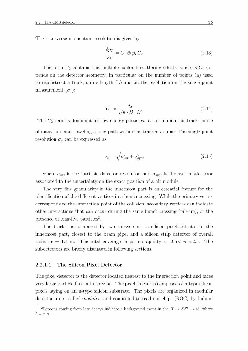
2.2. The CMS detector 35
The transverse momentum resolution is given by:
δpTpT
= C1 ⊗ pTC2 (2.13)
The term C2 contains the multiple coulomb scattering effects, whereas C1 de-
pends on the detector geometry, in particular on the number of points (n) used
to reconstruct a track, on its length (L) and on the resolution on the single point
measurement (σx):
C1 ∝σx√
n ·B · L2(2.14)
The C2 term is dominant for low energy particles. C1 is minimal for tracks made
of many hits and traveling a long path within the tracker volume. The single-point
resolution σx can be expressed as
σx =√σ2int + σ2
syst (2.15)
where σint is the intrinsic detector resolution and σsyst is the systematic error
associated to the uncertainty on the exact position of a hit module.
The very fine granularity in the innermost part is an essential feature for the
identification of the different vertices in a bunch crossing. While the primary vertex
corresponds to the interaction point of the collision, secondary vertices can indicate
other interactions that can occur during the same bunch crossing (pile-up), or the
presence of long-live particles2.
The tracker is composed by two subsystems: a silicon pixel detector in the
innermost part, closest to the beam pipe, and a silicon strip detector of overall
radius r = 1.1 m. The total coverage in pseudorapidity is -2.5< η <2.5. The
subdetectors are briefly discussed in following sections.
2.2.1.1 The Silicon Pixel Detector
The pixel detector is the detector located nearest to the interaction point and faces
very large particle flux in this region. The pixel tracker is composed of n-type silicon
pixels laying on an n-type silicon substrate. The pixels are organized in modular
detector units, called modules, and connected to read-out chips (ROC) by Indium
2Leptons coming from late decays indicate a background event in the H → ZZ∗ → 4`, where` = e, µ

2.2. The CMS detector 36
bump-bonds. It contributes precise tracking points in r, φ, z and therefore respon-
sible for a small impact parameter resolution that is important for good secondary
vertex reconstruction. The pixel system has a zero-suppressed analog pulse height
read-out scheme that improves position resolution and helps separating signal and
noise hits as well as identifying large hit clusters from overlapping tracks. To achieve
this resolution, a pixel cell size of 100×150 µm2 is utilized and the total number of
pixels is 47923200 in the barrel, 17971200 in the endcaps.
Figure 2.6: Hit coverage of the Silicon pixel detector.
The layout of the pixel system is shown in Fig. 2.6, where it consists of three
layers of pixel modules placed at radii of 4.4, 7.3 and 10.2 cm and two endcap
discs extending from 6 to 15 cm in radius placed at 34.5 cm and 46.5 cm from the
nominal interaction point. The pseudorapidity range covered is -2.5< η <2.5 and
the arrangement of the barrel layers and endcap disks ensures the existence of three
measurement points almost over full covered range.
2.2.1.2 The Silicon Strip Tracker
The particle flux is much lower outside the pixel detector so silicon micro-strip de-
tectors are utilized. The silicon strip tracker (SST) is displayed in Fig. 2.7 and
consists of three different sub-systems and 10 layers of silicon microstrip detectors.
The tracker inner barrel and disks (TIB/TID), extending in a radius of 55 cm, are
composed of four barrel layers and three disks at each end. The SST provides up to
4 r − φ measurements with a position resolution of 23 µm in the two inner layers
and 35 µm in the two outer layers. The TIB and TID are surrounded by the tracker
outer barrel system (TOB). TOB consists of 6 barrel layers, providing a resolution

2.2. The CMS detector 37
of 53 µm in the first four layers and 35 µm for the two outer layers.
Figure 2.7: Schematic cross section of the CMS silicon tracker. Each line correspondsto a detector module while double lines correspond to back to back modules.
It extends up to z = 118 cm and beyond this z range, the tracker endcaps
(TEC+,TEC-) provide the additional forward coverage up to η <2.5. Each TEC
provides 9 φ measurements per trajectory and extends to z = 282 cm. In addition
the first two layers of TIB/TID and TOB, as well as rings 1, 2 and 5 of the TEC,
carry a second micro-strip module with sensors in both sides with an angle of 100
mrad in order to provide a measurement of the second coordinate z or r in the barrel
and discs respectively. Both sub detectors have wedge shaped modules arranged in
rings, centered on the beam line, with strips pointing towards the beam line.
2.2.2 Electromagnetic Calorimeter
The calorimeters measure the energy of both neutral and charged particles. Elec-
trons, positrons and photons deposit all their energy through electromagnetic in-
teractions, by producing showers in the innermost calorimeter i.e. ECAL. It is a
hermetic homogeneous calorimeter, made of 61200 lead tungstate (PbWO4) crystals
mounted in the central barrel part accompanied by 7324 crystals in each of the two
endcaps.
The layout of the CMS ECAL is presented in Fig. 2.8 & 2.9. A preshower
detector is installed at the face of each of the two endcaps. Avalanche photo-diodes

2.2. The CMS detector 38
Figure 2.8: Layout of the CMS ECAL showing the arrangement of crystals, super-modules and endcaps with the preshower in front.
Figure 2.9: A schematic cross sectional diagram of the ECAL, showing the geo-metrical arrangement of the barrel ECAL, the endcap ECAL, and the preshowerdetector. The interaction point is located at the lower left edge of the diagram. Thedotted lines show the values of the pseudorapidity at the given angle.

2.2. The CMS detector 39
(APDs) are used as photo-detectors in the barrel and vacuum photo-triodes (VPT)
in the endcaps.
The choice of high density crystals allowed CMS to build a compact calorimeter
which provides fast response, high granularity and good energy resolution. The
design of the electromagnetic calorimeter is motivated by the search for Higgs bosons
in the di-photon final state where optimal position and energy resolution for photons
is essential for Higgs discovery.
2.2.2.1 Lead Tungstate Crystals
The choice of the material for crystals is very important for the performance of an
electromagnetic calorimeter. For precise measurement of the energy, leakage outside
the crystals has to be minimized. This is achieved by choosing a crystal material with
low radiation length and moliere radius. Lead tungstate crystals provide a radiation
length of 0.89 cm and their high density leads to a compact design resulting in 25.8
radiation lengths in 23 cm crystals. The position resolution is optimized by requiring
small transverse size of the electromagnetic shower.
The transverse profile of electromagnetic showers is expressed by the Moliere
radius3 About 90% of the electromagnetic energy of a shower lies within a cylinder
with radius equal to RM . The Moliere radius of the lead tungstate crystals is 2.2
cm and combined with a barrel crystal front face of 2.2×2.2 cm2 ensures that the
core of the shower will be included in a 2×2 crystal area. Lead tungstate provides
optimal scintillation time since about 80% of the light is emited in 25 ns which is
the nominal beam crossing time separation.
2.2.2.2 Calorimeter Resolution
For energies of electromagnetic showers below 500 GeV, where energy leakage from
the end of the calorimeter is negligible, the resolution of the electromagnetic calorime-
ter can be modeled in three terms:( σE
)2
=
(S√E
)2
+
(N
E
)2
+ C2, (2.16)
3The Moliere radius Rµ (RM ) is a characteristic constant of a material, giving the scale ofthe transverse dimension of the fully contained electromagnetic showers initiated by an incidenthigh energy electron or photon. It is defined as the mean deflexion of an electron of critical energyafter crossing a width 1X0, where X0 is defined as the radiation length, i.e. the average distancecovered by an electron in a material through which it loose a fraction of its energy equal to 1/e.A cylinder of radius Rµ contains on average 90% of the shower’s energy deposition.

2.2. The CMS detector 40
where S is the stochastic term, N is the noise term and C is constant term. The
stochastic term describes statistics related fluctuations such as intrinsic shower fluc-
tuations, photoelectron statistics, dead material in front of the calorimeter and
sampling fluctuations.
The main contribution to the constant term C are detector non-uniformity, cali-
bration uncertainty, radiation damage to the calorimeter and leakage from the out-
side of a crystal. The constant term can be reduced by utilizing radiation hard
media and performing in-situ calibration. The CMS calorimeter accounts for both
factors by utilizing a laser monitoring and calibration system.
The noise term is related to the electronics noise and estimated by measuring
the contribution from electronics noise after summing over some Moliere radii. One
additional noise factor can come from pile-up where remnant energy from a previous
crossing can be accounted in the measurement. The values of these three constants,
measured with test beams, are listed in Tab. 2.2.
Table 2.2: Contributions to the energy resolution of ECAL.
Contribution Barrel (η = 0) Endcap (η =2)
Stochastic term 2.7% 5.7 %Constant term 0.55 % 0.55%
Noise (low luminosity) 0.155 GeV 0.155 GeVNoise (high luminosity) 0.210 GeV 0.245 GeV
The crystals response depends strongly on their temperature, which must there-
fore be kept constant as a function of time. This is obtained with a cooling system
capable of collecting the heat dissipated by the read-out electronics and of ensuring
thermal stability. The nominal ECAL operating temperature is 18o.
2.2.3 The Hadron Calorimeter
The hadron calorimeter (HCAL) plays a major role in the detection of hadron jets,
especially the neutral ones since pions and kaons are detected by also estimating
their momenta with the silicon tracker. In addition, for adequate measurement of
the missing transverse energy, hermetic coverage is needed up to |η| <5. The CMS
HCAL is a brass/scintillator sampling calorimeter. It is mostly installed between the
ECAL and the solenoid magnet while its small part is installed outside the magnet
and it consists of four different subsystems:

2.2. The CMS detector 41
• Barrel Hadron Calorimeter (HB): located between ECAL barrel and the
magnet covering up to |η| <1.4.
• Endcap Hadron Calorimeter (HE): located inside the magnet, consisting
of two endcaps complementing HB and extending the coverage up to |η| <3.0.
• Outer Hadron Calorimeter (HO): located outside the magnet, in the bar-
rel using the magnet as additional absorber providing the additional absorber
length required for the barrel region.
• Forward Hadron Calorimeter (HF): placed 11.2 m from the nominal in-
teraction point extending the coverage from |η| >3 up to |η| <5.2.
The layout of the CMS HCAL is displayed in Fig. 2.10. The length scale of
hadronic calorimetry is designated as the interaction length (λI )4. The HB ab-
sorber consists of a 40 mm thick front steel plate, followed by eight 50.5 mm thick
brass plates, six 56.5 mm thick brass plates and a 75 mm thick steel plate. The total
absorber thickness at incident angle of 90o is 5.82λI while at η = 1.3 it is 10.6λI .
The electromagnetic calorimeter adds about 1.1 λI of additional material.
HF
HE
HB
HO
Figure 2.10: Longitudinal view of the CMS detector. The locations of the hadronbarrel (HB), the endcap (HE), the outer (HO) and the forward (HF) calorimeters.
4Nuclear interaction length is defined as the mean path length in which the energy of relativisticcharged hadrons is reduced by the factor of 1/e as they pass through matter.

2.2. The CMS detector 42
The endcap part uses the same absorber but the plates have a thickness of 79
mm. The plastic scintillator tiles are placed between the absorber layers, resulting
in 70000 tiles for the whole detector. The granularity of the tiles corresponds to
∆η × ∆φ of 0.087×0.087 in the range of |η| <1.6 and 0.17×0.17 in the region of
|η| >1.6. The HO utilizes the magnet as additional absorber corresponding to an
additional 1.4λI of material at normal incidence and it consists of two scintillator
layers with the same granularity as HB. The total depth in the central region sums
to about 11.8λI .
The light produced in the HB scintillators is transferred to the hybrid photo
diodes (HPDs) via optical fibers. HPDs consist of a photo-cathode held at a HV-8
kV at a distance of approximately 3 mm from a pixelated silicon photo-diode and
can provide a gain of 2000. The forward calorimeter (HF) design is very challenging,
since in the LHC environment on average 760 GeV of energy are deposited in the
forward calorimeters, compared to an average of 100 GeV in the rest of the detector.
This flux introduces the need for radiation hard design. CMS opted for a Cherenkov
based calorimeter using quartz fibers as an active material embedded in a steel ab-
sorber. The signal is generated when charged shower particles above the Cherenkov
threshold generate light that is captured by photo-multipliers tubes (PMT). The
HF is therefore more sensitive to the electromagnetic showers and some relativistic
charged pions.
In contrast to the electromagnetic calorimetry, in case of hadronic calorimetry,
the best achievable energy resolution is limited due to the nature of the hadronic
interactions. During a hadronic interaction, a part of the energy is purely electro-
magnetic due to the presence of πo and η mesons decaying to photon pairs and it
is measured directly by the photo-detectors. Charged particles, on the other hand
produce signal by ionization, excitation and nuclear interactions. In most of the
cases, a significant fraction of the energy of the order of 20 - 35%, deposited in a
sampling calorimeter is not visible resulting in degraded resolution. For the CMS
hadronic calorimeter, the resolution is described as:
( σE
)2
=
(99%√E
)2
+ (4.5%)2, (2.17)
for the HB, HO and HE and
( σE
)2
=
(172%√E
)2
+ (9.0%)2, (2.18)
for the HF.

2.2. The CMS detector 43
2.2.4 CMS Magnet
The CMS superconducting magnet provides a large bending power, allowing a pre-
cise measurement of the transverse momentum of charged particles. A further and
independent pT measurement outside the solenoid is possible due to the bending
power in the iron yoke. It has been designed to generate a uniform 3.8 T field in the
inner region, with a stored energy of 2.6 GJ at full current. The magnet is operated
at the temperature of 4 K, as low as to make a flat NiTb cable superconducting and
to produce a 20 kA current not subject to any appreciable loss. A vacuum cylinder
isolates the magnet from the external environment. A 10000 t return yoke closes the
B-field lines. It consists of 5 barrel layers and of 3 disks in each of the two endcaps.
The ratio between stored energy and cold mass is large (11.6 KJ/kg), which causes
a large mechanical deformation (0.15%) during the ramp-up phase. The parameters
of the CMS magnet are summarized in Tab. (2.3).
Table 2.3: A summary of the main features of the CMS magnet.
General Parameters
Eta Interaction length(λI)Magnetic Length 12.5 m
Cold bore diameter 6.3 mCentral magnetic induction 4 T
Total Ampere-turns 41.7 MA - turnsNominal current 19.14 kA
Inductance 14.2 HStored energy 2.6 GJ
Cold MassRadial thickness of cold mass 312 mm
Radiation thickness of cold mass 3.9 Xo
Weight of cold mass 220 tMaximum induction on conductor 4.6 T
Temperature margin wrt operating temperature 1.8 KStored energy/unit cold mass 11.6 kJ/kg
Iron JokeOuter diameter of the iron flats 14 m
Length of Barrel 13 mThickness of the iron layers in Barrel 300, 630, 630 mm
Mass of iron in Barrel 6000 tThickness of iron disks in Endcaps 250, 600, 600 mm
Mass of iron in each Endcap 2000 tTotal mass of iron in return yoke 10000 t

2.2. The CMS detector 44
2.2.5 The Muon System
The efficient and precise muon identification is one of the main requirements that
influenced the design of CMS detector. Muons have a lifetime of about 2.19 ×10⁻⁶s
[16], even longer at relativistic speed. Therefore they cross the full detector before
decaying. In addition, bremmstrahlung is suppressed by a factor of (me/mµ)2 with
respect to electrons for muons below 100 GeV, which implies that the muon does
not stop in the calorimeters but rather interacts via ionization. Muons are therefore
expected to produce a track in the CMS tracker and then escape the calorimeter
by depositing very small energy in it. In addition, for very energetic muons, the
tracker cannot provide sufficient momentum resolution. It creates the need of a
special muon system outside the calorimeters that can provide identification and
momentum measurement.
Figure 2.11: An r-z cross-section of a quadrant of the CMS detector with the axisparallel to the beam (z) running horizontally and radius (r) increasing upward. Theinteraction region is at the lower left corner. Shown are the locations of the variousmuon stations and the steel disks (red areas). The four drift tube (DT) stations arelabeled MB (“muon barrel”) and the cathode strip chambers (CSC) are labeled ME(“muon endcap”). Resistive plate chambers (RPC, in green) are in both the barreland the endcaps of CMS.

2.2. The CMS detector 45
The muon spectrometer has been designed to provide an efficient muon trigger
and a precise measurement of muon momentum and charge, even without relying
on information from the tracking system. Muon detectors are embedded in the iron
return yoke of the magnet, as shown in Fig. 2.11. Particles other than muons and
even muons with transverse momentum lower than ' 3 GeV, do not reach the muon
chambers. Three subsystems compose the spectrometer are explained below:
2.2.5.1 Drift Tube Chambers
In the CMS barrel, where the muon rate is under control, four layers of muon stations
are used, occupied by drift tube (DT) Chambers covering up to |η| <1.2; where the
residual magnetic field and the track occupancy are low. The DTs are divided in
five wheels along the z-coordinate, each including 12 azimuthal sectors. Along the
radial coordinate, four stations (MB1, MB2, MB3, MB4) are made of 12 chambers
each (see Fig. 2.11), one per φ sector, except for MB4, which contains 14 chambers.
The basic constituent of a DT chamber is a cell, as shown in Fig. 2.12, having
size of 42×13 mm2. A cell is bounded by two parallel aluminium planes and by
‘I − shaped′ aluminium beams serving as cathodes. The anodes are 50 µm stainless
steel wires located in the centre of the cells. Muons passing through a cell ionise the
gas mixture that fills the cell volume.
Figure 2.12: The individual drift tube cell and operation principle..

2.2. The CMS detector 46
The drift time of the resulting electrons is used to measure the distance between
the muon track and the wire. The linearity of relation between time and distance
is enhanced by means of an additional field shaping, given by two positively biased
insulated strips glued on the planes in correspondence to the wire.
The gas mixture within a cell is composed of Ar (85%) and CO2 (15%). It
guarantees good quenching properties and the saturation of the drift velocity, which
is ≈ 5.4 cm/µs. This corresponds to a maximum drift time of ≈ 390 ns, or 15 bunch
crossings. The efficiency of a single cell is ≈ 99.8%, its spatial resolution is ≈ 180
µm. Each chamber has a resolution of 100 µm in the r-φ plane and of ≈ 1 mrad
along the φ coordinate.
2.2.5.2 Cathode Strip Chambers
The cathode strip chambers (CSCs) are installed in the endcaps (see Fig. 2.11),
providing full muon coverage up to |η| <2.4. The CSCs are multi-wire proportional
chambers consisting of six planes of anode wires interleaved among seven cathode
panels. Wires run azimuthially, defining the tracks radial component, while strips
are equipped on cathode panels and run lengthwise at a constant ∆φ width.
Figure 2.13: Working principle of a CSC chamber.
The angular position φ of the track is estimated by extrapolating the charge that
is induced on the strips as shown in Fig. 2.13. The nominal gas mixture is 40 % Ar,

2.2. The CMS detector 47
50 % CO2 and 10 % CF4. The addition of CF4 is used to avoid polymerization of
the wires. The wires give very fast signals that provide very good time resolution.
A charged track passing through a chamber generates an avalanche that induces
a charge on several cathode strips which gives very good position resolution. By
interpolating among these strips one reaches a very fine spatial resolution of 50 µm.
The resolution along the φ coordinate is 10 mrad.
The CSCs consist of four stations (ME1 to ME4) as shown in Fig. 2.11, the
innermost one including three concentric rings, the other ones only two. The inner
rings of stations ME2 to ME4 contain 18 chambers, all the other ones include 36
chambers. The CSCs can operate at high rates and in large and non-uniform mag-
netic fields without requiring precise monitoring of gas, pressure or temperature and
can provide trigger and precision position measurement in the same device.
2.2.5.3 Resistive Plate Chambers
The resistive plate chambers (RPC) are gaseous parallel plate detectors that com-
bine adequate position resolution with very high speed. RPCs are located both in
the barrel and in the endcaps as displayed in Fig. 2.11, which covers |η| <2.1.
Figure 2.14: A schematic diagram of the RPC double gap chamber.
Their spatial resolution is limited, but their time resolution is very good, about 1
ns, a shorter time than the 25 ns i.e. LHC bunch spacing. Therefore RPC detectors
are used to identify unambiguously a bunch crossing and to provide prompt trigger
decisions. RPCs are made of two parallel plates of bakelite, a high-resistivity plastic
material, with a few mm thick gas gap in between them and a graphite coat outside

2.2. The CMS detector 48
of them and shown in Fig. 2.14. Aluminum strips, separated from the graphite
layers by an insulating PET (polyethylene terephtalate) film, read out the signals.
The gas mixture filling the gap consists of C2H2F4 (95%) and of i-C4H10(5%).
The geometrical layout of the RPC chambers depends on their position. In the
barrel region, six layers of RPCs are there: four of them are attached to each side of
the MB1 and MB2 DT chambers, the other two to the inner side of MB3 and MB4.
In the endcaps, four disks of trapezoidal RPC are attached to the CSCs.
2.2.6 Trigger System and Data Acquisition
The trigger system and integrated data acquisition (DAQ) is active in CMS to record
data quickly and efficiently. The LHC provides proton collisions at high interaction
rates with a designed bunch crossing rate of 40 MHz. Each recorded event in CMS
has a nominal size of 0.5 -1MB which makes impossible to store and process this
huge number of events.
Therefore, a drastic rate reduction is achieved in real time using the trigger
system. In CMS, this is achieved by splitting the whole workflow in three steps or
‘levels′: L1, L2, L3. Each of them reads out and processes only a limited fraction
of the available information. The level-one step is totally hardware-based, whereas
L2 and L3 are sets of software requirements and are usually referred to as high level
trigger (HLT). The HLT algorithm takes as input relatively few events, therefore it
can analyze them in a more detailed way.
2.2.6.1 The Level-1 Trigger
The L1 Trigger uses coarse information from the calorimeter and the muon system,
while holding the high resolution data in pipelined memories in the front-end elec-
tronics until the trigger decision is taken. It consists of mostly custom-designed,
programmable hardware capable of bringing down the event rate from the initial 40
MHz to 100 kHz. The maximum allowed latency is 3.2 µs, after which, if the L1
accepts the event, the data starts being processed by the HLT. Since it would not
be possible to read out and analyze the whole information contained in an event,
mostly because of the time needed by tracking algorithms, only calorimeters and
muon chambers are involved in the L1 step, as shown in Fig. 2.15.
The calorimeter trigger finds out the four ‘best’ candidates of each of the following
categories: electrons and photons, central jets, forward jets and jets identified on
the basis of the shape of the deposited energy. These candidates are handed over to
the global calorimeter trigger (GCT), along with the measured missing transverse

2.2. The CMS detector 49
energy.
The muon trigger is performed independently by DTs, CSCs and RPCs. The
DT and CSC triggers carry out a local muon reconstruction by comparing the slopes
of track segments built in subsequent detector layers. The RPC trigger compares
a given muon track with predefined hit patterns depending on the track pT . The
four best muon candidates are passed to the global muon trigger system, which is
in charge of matching those from DTs and CSCs with those from RPCs and of
discarding low-quality tracks. The L1 electronics is installed partly directly on the
detectors, partly in the underground control room about 20 m far from the experi-
mental cavern.
Figure 2.15: Schematic representation of the CMS L1 trigger system.
2.2.6.2 The High Level Trigger
The HLT is a software system running on a farm of about 1000 commercial proces-
sors, designed to reduce the event rate down to the final output of ≈100 Hz that can
be written on tape. The HLT processes all events accepted by the Level-1 trigger in
a single processor farm. The reconstruction and selection in the HLT takes place in
steps and the selection is optimized step by step in order to reject events as quickly

2.2. The CMS detector 50
as possible.
The basic idea is to reconstruct those part of each physics object that can be
used for selection while minimizing the overall CPU usage e.g. the reconstruction of
a muon includes the reconstruction of a track in the muon spectrometer, the search
of a matching tracker track, and the global track reconstruction. After each step, a
set of selection criteria results in the rejection of a significant fraction of the events
accepted by the previous step, which results in to reduction of required CPU time
for forthcoming steps. Reconstruction and selection are therefore closely intertwined
in the online environment of the filter farm.
As a convention, the term Level-2 Trigger is used to refer to algorithms and
requirements of the first selection step in the HLT process. Typically, a Level-2
trigger, which has the full Level-1 rate as input, uses only information from the
calorimeter and muon detectors. In contrast, Level-3 Trigger refers to a further
selection step that includes the reconstruction of full tracks in the tracker. Because
of the high number of channels, the complex pattern recognition and higher combi-
natorics, track reconstruction is a process that demands large amount of CPU time.
Thus tracker-tracks are used only for the Level-2 pre-selected events.
The CMS detector hosts partial reconstruction of the information to minimize the
CPU time required by the HLT. In many cases, the event acceptance decision by the
HLT involves the reconstruction of quantities in only a limited region of the detector
e.g. for an event accepted by the Level-1 trigger in the inclusive muon stream, only
the parts of the muon chambers indicated by the Level-1 trigger results, and the
corresponding region in the tracker, need to be considered for the validation of the
muon. In HLT, the reconstruction of physics object is driven by the corresponding
candidates identified by the Level-1 trigger. This approach leads to significant CPU
savings.
A list of reconstruction algorithms and filters for one or more physics objects that
starts any time, a Level-1 bit is enabled is called HLT path. For each luminosity
scenario the set of trigger paths that, if enabled, contribute to a final OR of decisions
which determines whether to reject or store an event, is called HLT Menu. A single
trigger path can require the presence of one or more physics objects of a particular
type that pass specific kinematic thresholds, and it can also mix different type of
physics objects (cross triggers). The rate of expected events for a particular set of
trigger paths given a luminosity scenario is studied on simulation. By increase in
luminosity, the requirements on the trigger paths are becoming more stringent due
to rate constraints, and the selection algorithms becomes more complex to cope with
the requests of each physics analysis. Trigger paths with lower threshold than those

2.2. The CMS detector 51
necessary to face the event rate are kept in the HLT Menu with a prescale factor
applied. This is done to have on storage the data sample required to measure and
monitor the efficiency of the higher threshold trigger paths.
2.2.6.3 The Data Acquisition System
The CMS data acquisition (DAQ) is responsible for conveying the data from about
650 read-out modules to the filter units that will process the events. Each module
provides event fragments with a size of ≈ 2 kB. The CMS DAQ structure is outlined
in Fig. 2.16. The detector sensors are read out by the so-called Front−End Drivers(FEDs) through a builder network having a bisectional bandwidth of 100 GB/s. The
FEDs are situated in the underground counting room, ≈ 70 m far from the detector.
Events are passed to the event filter systems at a maximum rate of 100 kHz. This
large rate, corresponding to the L1 one, is due to the design choice of building the
full event already after the L1 trigger stage, unlike in the standard multi-level trigger
systems.
Figure 2.16: The structure of the CMS DAQ system.

2.2. The CMS detector 52
2.2.7 CMS Computing Model
One of the great challenge for the CMS experiment is to manage the data storage
and computational resources that are needed to achieve the physics goals of the
experiment. The data volume that the experiment collects, and the computing re-
sources that are needed to analyze the data are more than an order of magnitude
larger than previous high energy physics experiments. The development of grid com-
puting in the past ten years have allowed the choice of distributed computing as a
solution to meet the challenge. The CMS computing model partitions the aggregate
computing resources into three different tiers that serve specific purposes.
Figure 2.17: Overview of CMS computing framework.
The Tier-0 center consists of a single large computing farm along with a mass
storage system situated at the CERN Meyrin site. It is responsible for receiving
the raw data from the storage manager system and converting it into the RAW
data format to be stored permanently on the mass storage system at CERN. It also
performs a prompt reconstruction, using the best available information on calibra-
tion and alignments at the time. The first copy of the RAW data and the prompt
reconstruction is stored at the Tier-0 for custodial storage. A second permanently
stored copy is transferred to one pre-designated Tier-1 site for custodial archiving.
The eight Tier-1 centers currently in existence serve primarily two purposes.
The first purpose is to archive the custodial copy of the data on their tape mass

2.2. The CMS detector 53
storage systems. The second purpose is to provide computing resources for repro-
cessing of the data. As a result, the Tier-1 sites are almost exclusively used for this
purpose and analysis activities are severely restricted.
The roughly fifty Tier-2 centers are primarily dedicated to performing physics
analysis. They do not have any tape storage systems and have limited storage space.
Roughly 50% of the computing resources of the Tier-2 centers are used for centralized
monte carlo production, while the remaining resources are for user analysis. The
centrally produced monte carlo data samples are subsequently transferred to a pre-
designated Tier-1 center for custodial storage.

2.2. The CMS detector 54

Chapter 3
Event Simulation and
Reconstruction
The physics and detector simulation is necessary in high energy physics to model
complex physics processes, optimize analysis techniques and comprehend the per-
formance of the numerous and complex sub-detectors of an apparatus such as CMS.
Physics event generation and detector response simulation is performed using the
monte carlo (MC) method [17]. The MC method uses random sampling applied to
a theoretical model to predict its expected behavior in realistic conditions. It relies
on computer simulations and can give correct solutions especially in cases where a
deterministic solution cannot be derived.
Examples in high energy physics include event simulation where particles are
produced in random direction and position but obey the theoretical constraints and
also detector simulation, where the detector behavior during passage of particles
through it, is modeled precisely including any external parameters such as elec-
tronic noise, noise of neighboring sub-detectors and other effects (e.g. temperature
changes).
3.1 Physics Event Generation
The first step in the simulation process is the event generation, which refers
to the procedure of simulating a collision using programs known as MC generators
[18]. It is usually performed in many steps following a modular approach, often
using different MC programs for each step.
55

3.1. Physics Event Generation 56
3.1.1 Hard Scattering Process
The event generation is initiated by simulation of the hard scattering process. To
illustrate the generation process we assume Z production at tree level and decay to
lepton pairs, pp → Z → ``. This process has a matrix element M(qq → Z → ``)
and the total cross section taking into account the parton distribution functions is:
dσ =1
3fqfq
1
2(xys)2|M(qq → Z → ``)|2 dcosθ dφ dx dy
8(2π)2(3.1)
where fq, fq are the parton distribution functions of the proton for each quark q
and s is the square of the center of mass energy of the LHC, where√s= 7 & 8 TeV
in accord with present analysis. The momentum fractions that each quark carries
from the original proton are denoted as x and y. For the calculation of the cross
section, eq. 3.1 is integrated using MC method by picking uniform random numbers
(θ, φ, x, y, q) and calculating the average < dσ > which is an approximation of the
cross section integral. Each element dσ is referred to as the event weight.
In case of the event generation, the purpose is not the calculation of the cross
section but the creation of particles produced by a random collision due to the pro-
cess under test, in this case Z production. To achieve this goal, the maximum event
weight dσMAX is calculated by scanning the phase space and then each infinitesimal
element dσ is normalized by calculating dσ/dσMAX . For each candidate event, the
ratio of event weight over the maximum event weight dσ/dσMAX is compared to a
random number g generated uniformly in the interval (0,1). Events for which the
ratio exceeds the random number (dσ/dσMAX > g) are accepted; the others are
rejected. Before the output is converted to particles that will be simulated within
the detector, additional processes, e.g. NLO effects, (radiation of gluons, quarks
and photons ), evolution of jets (explained in succeeding section as hadronization)
etc. need to be performed.
3.1.2 Parton Shower, Underlying Event and Hadronization
The next step is to add higher order effects by ‘evolving’ the event using par-
ton shower simulation, which allows partons to split in pairs of other partons
(i.e g → qq, q → gq). The resulting partons can branch further, resulting in a
large number of final quarks and gluons that are not allowed to exist in isolation
due to color confinement. The succeeding act is the modeling of the underlying

3.1. Physics Event Generation 57
event (UE). The UE refers to the beam remnants of the proton after the partons
contributing to the hard scattering have been pulled out. The beam remnants recoil
against a very small transverse momentum, present due to the motion of the partons
inside the proton. The resulting partons are then grouped together into color sin-
glet composite hadrons using a phenomenological model known as ‘hadronization’.
Fig. 3.1 shows the different steps in the event generation by using an example of a
proton collision resulting in two quarks followed by parton shower and hadronization.
Figure 3.1: The basic structure of a showering and hadronization generator event isshown schematically.
The hadronization scale is in the non-pertubative regime. Therefore, crude phe-
nomenological models which contain several parameters tuned with experimental
data are used. The impact of the choice of the hadronization model is small for
most physics processes because the hadronization scale is much smaller than the
hard scales. Any resonances created during the hadronization process are decayed.
Finally the possibility of multi-parton interactions where two or more partons per
proton can interact is taken into account and is added to the simulated event.

3.1. Physics Event Generation 58
3.1.3 MC Generator Programs
Several MC simulation programs are used to model the SM Higgs signal and back-
ground processes in this analysis according to the peculiarities of the different final
states under study. A brief description of the respective generators is described in
the following sections.
3.1.3.1 PYTHIA
PYTHIA is a general multi-purpose MC event generator for lepton and hadron col-
liders and discussed in Ref. [19]. It consists of a sub-process library containing about
240 different 2 → n sub-processes, all at leading order. The standard processes in-
clude SM vector boson and vector boson pair production, QCD multijet production,
SUSY, Higgs production and exotic physics. Initial and final state showers are added
to provide more realistic configurations especially for the internal structure of jets.
The hadronization is also performed by using a phenomenological model known
as the ‘Lund model’ and the underlying event is simulated by 2 → 2 scatterings
between the remaining partons. PYTHIA serves either to generate a given hard
process at leading order (LO), or, in cases where the hard processes are generated
at higher orders, it is used only for the showering, hadronization, decays, and for
adding the underlying event; the parton shower and hadronization code developed
for PYTHIA is also used when interfaced to other generators such as POWHEG
and MadGraph [20] [23].
3.1.3.2 POWHEG
The POWHEG program is an improvement to PYTHIA since it utilizes NLO cal-
culations combined with parton shower. The main idea of the POWHEG method is
that the hardest emission (the one with the highest pT ) is simulated in accord with
the exact NLO cross section. The hardest emission is excluded during the parton
shower and subsequent emissions are vetoed if they are harder than the hardest
emission. The POWHEG method provides a much better description of basic pro-
cesses as compared to PYTHIA, such as vector boson and SM Higgs production and
is used explicitly to describe final states with low multiplicity such as inclusive W/Z
production. In addition, the tt → 2`2ν2b samples are generated with POWHEG
by using the CTEQ6M PDF [24] and it has been also used for generation of ‘single
top’ [25] and qq → ZZ∗ → 4` background processes.

3.1. Physics Event Generation 59
3.1.3.3 gg2ZZ
The gg2ZZ is used to generate the gg → ZZ → 4` (see Fig. 1.7b) contribution to
the ZZ cross section, which provides an important background for the SM Higgs
boson searches in the H→ZZ channel at the LHC. It calculates the loop-induced
gluon-fusion process gg→ Z∗(γ∗)Z∗(γ∗) → ` ¯′ ¯′ and discussed in Ref. [21].The
gg-induced process yields a correction of about 15% (at√s = 14 TeV) relative to
the NLO QCD prediction for the qq-induced process when only a M``, M`′ ¯′ > 5
GeV cut is applied. The gg→ ZZ∗ → 4` events are then showered and hadronized
using PYTHIA.
3.1.3.4 MADGRAPH
MADGRAPH program is used to generate multi-parton amplitudes and events for
some important background processes. One example is the WZ+jets background in
current analysis where one lepton is produced from the W decay, 2 leptons from Z
decay and one jet is eventually faking a 4th lepton.
PYTHIA is very effective when describing simple 2→ 2 processes but with mul-
tiple partons, MadGraph generator provides a better description for final states with
multiple partons utilizing calculations of diagrams of multiple final state objects at
tree level. Given a user process, MadGraph automatically generates the amplitudes
for all relevant sub-processes and produces the mappings for the iteration over the
phase space. Once the events are generated, they are passed to PYTHIA for the
parton shower and hadronization procedures. MadGraph has been used to produce
‘W + jets’, Z + jets (m`` > 50), Z + jets (10 < m`` < 50), WW → 2`2ν and WZ
→ 3`ν background processes.
3.1.4 K-factors
Even if event generators are becoming more and more sophisticated, there are usually
several calculations performed in higher orders that affect observable quantities in
the experiment. To account for those additional effects, the specific observables of
a generator are re-weighted to match the spectra of the observables of the higher
order calculation. The weights that are produced via this process are referred as
‘K-factors’. One example is the re-weighting of the pT of the Higgs boson to match
the spectrum obtained by NNLO calculations.

3.2. Detector Simulation 60
3.2 Detector Simulation
The complexity of the CMS Detector requires very sophisticated simulation to
properly reproduce the detector behavior in the presence of particles from proton
collisions. The detailed simulation is performed using the GEANT4 [22] toolkit.
GEANT4 relies on the accurate detector description including the full geometry,
the materials of the detecting devices and the dead material (e.g. cables, support,
cooling ) to simulate the particle response.
It takes input as particles from the event generator and then propagates them
through the detector taking into account the measured magnetic field map (for
charged particles) and any interactions between particle and material such as bremm-
stralung, multiple scattering and photon conversions. At the final stage, GEANT4
produces a set of simulated hits in the active material such as the energy loss of a
particle in the sensitive volume of a detector. The simulated hits are then fed to
emulators of the readout and trigger electronics to simulate the event and provide it
in digitized format which is equivalent to the digital information produced by real
data events. All subsequent stages, such as event reconstruction, use the same input
collection and are the same when running on simulated events or data.
3.2.1 Simulation of Multiple Interactions
The number of interactions per crossing can significantly affect the performance
of identification of interesting events. Therefore, the effects of pileup need to be
simulated properly to account for the changes in performance and allow for studies
to improve the performance for operation on higher luminosities. Pileup is simulated
by over-laying events at the hit level.
The hard interaction events are mixed with additional simulated minimum bias
events 1 by combining the hits between them. Both in-time (multiple vertices per
event) and out-of-time (detector response remnants from previous crossings) are
simulated. For out-of-time pileup, the time information is shifted by one bunch
crossing allowing the slower detectors to be affected by the information in the other
crossings. Along with the simulated hits, the generator information is also provided
to allow for studies of the merged event.
The distribution of pile-up interactions in the data depends on the run period
and the respective LHC configuration. However, the production of the simulated
1Minimum bias is a generic term which refers to events that are selected with a ‘loose’ triggerthat accepts a large fraction of the overall inelastic cross section. All triggers produce some biasand the term ‘minimum bias’ is meaningful when one specifies the precise trigger used to collectthe data.

3.3. Datasets and Triggers 61
samples is performed centrally before or during the data collection. To avoid multiple
simulation production runs, the simulated samples are produced with a poissonian
distribution of pile up interactions and that distribution is re-weighted to match the
distribution of interactions in data.
3.3 Datasets and Triggers
3.3.1 Experimental Data
The analysis relies on data samples which are centrally organized in primary datasets
(PDs) and its definition in terms of HLT paths (see Sec. 2.2.6.2) has been changing
along with the increasing instantaneous luminosity delivered by the LHC. The data
sample used in this analysis was recorded by the CMS experiment during 2011 for
the run range from 160431 to 180252 and during 2012 for the run range from 190645
to 203002.
In other words, the analysis has been performed over data collected in years
2011 (L = 5.05 fb−1 @√s = 7 TeV) and 2012 (L = 12.21 fb−1 @
√s = 8 TeV).
The absolute pp luminosity is known with a precision of 2.2% in 2011 and 4.4% in
2012. The CMS standard selection of runs and luminosity sections is applied which
requires high quality data with a good functioning of the different sub-detectors.
Thus, similar detector operation conditions are imposed for the validation of the
data to be used for the analysis of the 4e, 4µ and 2e2µ channels.
For the 2011 data, the analysis relies on the so-called ‘DoubleElectron’ and ‘Dou-
bleMuon’ PDs [26]. These latter PDs are formed by an ‘OR’ between various trigger
selections with symmetric or asymmetric trigger thresholds for the two leptons, with
or without additional identification and isolation requirements. They also include
triggers requiring three leptons above a low pT threshold.
In 2012, electron-muon cross-triggers are added to recover few percent of ineffi-
ciency in the 2e2µ channel at low Higgs boson masses, forming the so-called ‘MuEG’
PDs. In addition, tri-electron triggers for both 2011 and 2012 data has been used.
The PDs and trigger paths used for this analysis are summarized in Tab. 3.1 and
corresponds to different data taking periods. Tab. 3.2 shows all the trigger paths
used with 2012 data. The naming convention of trigger paths displays the infor-
mation about set of selection cuts used, named as very loose (VL), tight (T), very
tight (VT) over lepton’s isolation (Iso), identification (Id) in calorimeters (Calo) and
trackers (Trk). Some additional comments:
• In 2011, when applying double muon triggers other then HLT_Mu17_Mu8 one

3.3. Datasets and Triggers 62
has to require 2 offline reconstructed muons having pT > 17 GeV and pT > 8
GeV.
• While running on data, 4µ channel is obtained from DoubleMu datasets, 4e
channel is obtained from DoubleElectron datasets and 2e2µ channel have been
obtained from DoubleElectron & DoubleMu PDs by vetoing DoubleElectrons
triggers for 2011 data, while for 2012, MuEG dataset has been used in addition
by vetoing DoubleElectrons and DoubleMuons triggers.
Table 3.1: Datasets and trigger paths used in the analysis.CaloTrk = CaloIdT CaloIsoVL TrkIdVL TrkIsoVL
Datasets2011 2012/DoubleElectron/Run2011A-16Jan2012-v1 /DoubleElectron/Run2012A-13Jul2012-v1/DoubleMu/Run2011A-16Jan2012-v1 /DoubleMu/Run2012A-13Jul2012-v1/DoubleElectron/Run2011B-16Jan2012-v1 /MuEG/Run2012A-13Jul2012-v1//DoubleMu/Run2011B-16Jan2012-v1 /DoubleElectron/Run2012A-recover-06Aug2012-v1
/DoubleMu/Run2012A-recover-06Aug2012-v1/MuEG/Run2012A-recover-06Aug2012-v1/DoubleElectron/Run2012B-13Jul2012-v1/DoubleMu/Run2012B-13Jul2012-v4/MuEG/Run2012B-13Jul2012-v1/DoubleElectron/Run2012C-24Aug2012-v1/DoubleElectron/Run2012C-PromptReco-v2/DoubleMu/Run2012C-24Aug2012-v1/DoubleMu/Run2012C-PromptReco-v2/MuEG/Run2012C-24Aug2012-v1/MuEG/Run2012C-PromptReco-v2
Muon triggersHLT_DoubleMu7 HLT_Mu17_Mu8
OR HLT_Mu13_Mu8
OR HLT_Mu17_Mu8
Electron triggersHLT_Ele17_CaloTrk_Ele8_CaloTrk HLT_Ele17_CaloTrk_Ele8_CaloTrk
OR HLT_Ele17_CaloTrk_Ele8_CaloTrk HLT_Ele15_Ele8_Ele5_CaloIdL_TrkIdVL
OR HLT_TripleEle10_CaloIdL_TrkIdVL
Cross triggersHLT_Mu17_TkMu8
OR HLT_Mu8_Ele17_CaloTrk
OR HLT_Mu17_Ele8_CaloTrk
Integrated luminosity5.05 fb−1 12.21 fb−1
3.3.2 Simulated Samples
The SM Higgs boson signal samples, as well as samples for a large variety of elec-
troweak and QCD-induced SM background processes, have been obtained using de-
tailed MC simulations. All datasets were subject to full reconstruction. The signal
and background samples have been used for the optimization of the event selection
strategy prior to the analysis of the experimental data (see Sec. 3.5). They are
further used in this analysis for the comparisons with the measurements, the evalu-
ation of acceptance corrections and systematics, and for the background evaluation

3.3. Datasets and Triggers 63
Table 3.2: Trigger selections in 2012 data analy-sis. CaloTrk=CaloIdT CaloIsoVL TrkIdVL TrkIsoVL andCaloTrkVT=CaloIdVT CaloIsoVT TrkIdT TrkIsoVT
# Channel Purpose HLT path L1 seed prescale
4e main HLT_Ele17_CaloTrk_Ele8_CaloTrk L1_DoubleEG_13_7 1HLT_Ele15_Ele8_Ele5_CaloIdL_TrkIdVL L1_TripleEG_12_7_5 1
4µ main HLT_Mu17_Mu8 L1_Mu10_MuOpen 1OR HLT_Mu17_TkMu8 L1_Mu10_MuOpen 1
2e2µ main HLT_Ele17_CaloTrk_Ele8_CaloTrk L1_DoubleEG_13_7 1OR HLT_Mu17_Mu8 L1_Mu10_MuOpen 1OR HLT_Mu17_TkMu8 L1_Mu10_MuOpen 1OR HLT_Mu8_Ele17_CaloTrk L1_MuOpen_EG12 1OR HLT_Mu17_Ele8_CaloTrk L1_Mu12_EG6 1
Trigger paths used for lepton’s measurements via tag & probe method [28], [29]
4e and 2e2µ Z T&P HLT_Ele17_CaloTrkVT_Ele8_Mass50 L1_DoubleEG_13_7 54e and 2e2µ Z T&P low pT HLT_Ele20_CaloTrkVT_SC4_Mass50_v1 L1_SingleIsoEG18er 104µ and 2e2µ Z T&P HLT_IsoMu24_eta2p1 L1_SingleMu16er
4µ and 2e2µ J/psi T&P HLT_Mu7_Track7_Jpsi
HLT_Mu5_Track3p5_Jpsi
HLT_Mu5_Track2_Jpsi
procedure where measurements in a ‘background control’ region are extrapolated to
the ‘signal’ region. The various type of backgrounds contributing in current analysis
has been briefly discussed in Sec. 1.4.
The individual Monte Carlo simulation datasets used for this analysis has been
summarized in Tab. 3.3 along with MC simulation programs and respective cross-
sections. All the signal and background processes cross sections are re-weighted to
the NLO. In the case of SM Higgs boson production via the gluon fusion mechanism,
the most recent NNLO+NNLL calculations of the cross sections are included in Ref.
[27]. More details on the event generators and the background samples used in this
analysis, as well as indications on the procedures used to re-weight the MC events
where needed, are provided in the following section.
3.3.2.1 Signal: H→ ZZ∗ → 4`
The Higgs boson samples used in the current analysis are generated with POWHEG
which incorporates NLO gluon fusion (gg → H) and vector boson fusion qq → qqH.
The CTEQ6M parton distribution (PDF) set is used for generation with the Higgs
boson widths taken from Ref. [27]. Additional samples with WH, ZH and ttH
associated production are produced with PYTHIA. The Higgs boson is forced to decay
to two Z-bosons, which are allowed to be off-mass shell, and both Z-bosons are forced
to decay via Z → 2`. Generator level events are re-weighted according to the total
cross section σ(pp→ H) which comprises the gluon fusion contribution up to NNLO
and NNLL taken from Refs. [27, 33, 34, 35, 36, 37, 38, 39, 41, 42] and the weak-boson
fusion contribution at NNLO computed in Refs. [27, 43, 44, 45, 46, 47] The total
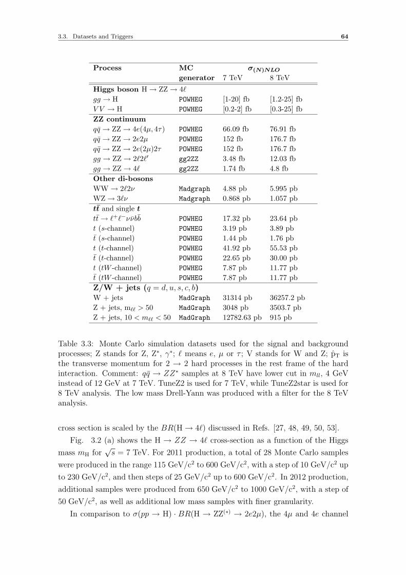
3.3. Datasets and Triggers 64
Process MC σ(N)NLO
generator 7 TeV 8 TeV
Higgs boson H→ ZZ→ 4`gg → H POWHEG [1-20] fb [1.2-25] fbV V → H POWHEG [0.2-2] fb [0.3-25] fbZZ continuumqq → ZZ→ 4e(4µ, 4τ) POWHEG 66.09 fb 76.91 fbqq → ZZ→ 2e2µ POWHEG 152 fb 176.7 fbqq → ZZ→ 2e(2µ)2τ POWHEG 152 fb 176.7 fbgg → ZZ→ 2`2`′ gg2ZZ 3.48 fb 12.03 fbgg → ZZ→ 4` gg2ZZ 1.74 fb 4.8 fbOther di-bosonsWW→ 2`2ν Madgraph 4.88 pb 5.995 pbWZ→ 3`ν Madgraph 0.868 pb 1.057 pbtt and single ttt→ `+`−ννbb POWHEG 17.32 pb 23.64 pbt (s-channel) POWHEG 3.19 pb 3.89 pbt (s-channel) POWHEG 1.44 pb 1.76 pbt (t-channel) POWHEG 41.92 pb 55.53 pbt (t-channel) POWHEG 22.65 pb 30.00 pbt (tW -channel) POWHEG 7.87 pb 11.77 pbt (tW -channel) POWHEG 7.87 pb 11.77 pbZ/W + jets (q = d, u, s, c, b)W + jets MadGraph 31314 pb 36257.2 pbZ + jets, m`` > 50 MadGraph 3048 pb 3503.7 pbZ + jets, 10 < m`` < 50 MadGraph 12782.63 pb 915 pb
Table 3.3: Monte Carlo simulation datasets used for the signal and backgroundprocesses; Z stands for Z, Z∗, γ∗; ` means e, µ or τ ; V stands for W and Z; pT isthe transverse momentum for 2 → 2 hard processes in the rest frame of the hardinteraction. Comment: qq → ZZ∗ samples at 8 TeV have lower cut in mll, 4 GeVinstead of 12 GeV at 7 TeV. TuneZ2 is used for 7 TeV, while TuneZ2star is used for8 TeV analysis. The low mass Drell-Yann was produced with a filter for the 8 TeVanalysis.
cross section is scaled by the BR(H→ 4`) discussed in Refs. [27, 48, 49, 50, 53].
Fig. 3.2 (a) shows the H → ZZ → 4` cross-section as a function of the Higgs
mass mH for√s = 7 TeV. For 2011 production, a total of 28 Monte Carlo samples
were produced in the range 115 GeV/c2 to 600 GeV/c2, with a step of 10 GeV/c2 up
to 230 GeV/c2, and then steps of 25 GeV/c2 up to 600 GeV/c2. In 2012 production,
additional samples were produced from 650 GeV/c2 to 1000 GeV/c2, with a step of
50 GeV/c2, as well as additional low mass samples with finer granularity.
In comparison to σ(pp → H) · BR(H → ZZ(∗) → 2e2µ), the 4µ and 4e channel

3.3. Datasets and Triggers 65
[GeV]HM
100 200 300 400
[fb]
4l
→ Z
Z*
→ H
→
pp
σ
0
1
2
3
4
5
6
7
8
-e+e-e+ e→H
)µ (l=e,-l+l-l+ l→H
-µ+µ-e+ e→H
(a)
[GeV]HM100 200 300 400 1000
4f)
ff) /
Br(H
(V
2
Br
× V
V)
Br(H
0.7
0.8
0.9
1
LHC
HIG
GS
XS W
G 2
010
-e+e-e+ eH
-µ+µ-e+ eH
)µ (l=e,-l+l-l+ lH
[GeV]HM100 200 300 400 1000
4f)
ff) /
Br(H
(V
2
Br
× V
V)
Br(H
0.95
1
1.05
1.1
LHC
HIG
GS
XS W
G 2
010
e - ee + eH
µ -µ e + eH
),µ,e
=, µ (l=e, - l + lH
[GeV]HM100 200 300 400 1000
4f)
ff) /
Br(H
(V
2
Br
× V
V)
Br(H
0.96
0.98
1
1.02
1.04
LHC
HIG
GS
XS W
G 2
010
q=udscb)µ (l=e,qq-l+ lH
q=udscb)µ (l=e,qq± lH
[GeV]HM100 200 300 400 1000
4f)
ff) /
Br(H
(V
2
Br
× V
V)
Br(H
0.96
0.98
1
1.02
1.04
LHC
HIG
GS
XS W
G 2
010
, q=udscb),µ,e= (qq H
(q=udscb)qqq qH
(b)
Figure 3.2: Cross-section for SM Higgs in H→ 4`, H→ 2e2mu and H→ 4e (or 4µ)as a function of mH in pp collisions at
√s = 7 (a). Cross-section enhancement due
to the interference of amplitudes with permutations of identical leptons originatingfrom different Z-bosons, as a function of mH (b).
cross-sections are enhanced in the case of off-shell Z boson due to an interference
of amplitudes with permutations of identical leptons originating from different Z-
bosons, as shown in Fig. 3.2 (b). This is correctly taken into account by Prophecy4f,
discussed in Refs. [27, 48, 49].
The POWHEG MC program used to simulate the gg → H process results in a Higgs
boson pT spectrum that differs significantly from the best theoretical calculation
which is available at NNLL+NLO. A theoretical estimate of this pT spectrum is
computed using the HqT [51] program, which implements such NNLL+NLO calcu-
lation. A re-weighting procedure has been studied to be applied to the simulated
events but the effect is very small for this analysis in which no direct constraints are
imposed on the transverse momentum of the 4` system, or on the hadronic recoil
against this system (e.g. no jet veto or missing transverse momentum cut).
In the current analysis, only samples for gluon fusion production mechanism
have been used and rescaled to the total cross section including all other production
processes (weak-boson fusion, WH, ZH and ttH associated production).
3.3.2.2 Background: qq → ZZ∗ → 4`
The qq → ZZ∗ → 4` samples have been produced with POWHEG, that include the
complete NLO simulation, interfaced to PYTHIA for showering, hadronization, decays
and the underlying event.

3.3. Datasets and Triggers 66
3.3.2.3 Background: gg → ZZ∗ → 4`
The gluon-induced ZZ background, although technically of NNLO compared to the
first order Z-pair production, amounts to a non-negligible fraction of the total irre-
ducible background at masses above the 2MZ threshold. A full NNLO calculation for
the ZZ production which would also take these gluon-induced diagrams into account
is not available. Therefore the contributions are estimated by using the dedicated
tool gg2ZZ, which computes the gg → ZZ at LO, which is of order α2s , compared
to α0s for the LO qq → ZZ. The hard scattering gg → ZZ∗ → 4` events are then
showered and hadronized using PYTHIA.
The gg2ZZ tools provide the functionality to compute the cross-section after
applying a cut on the mimimally generated invariant mass of the same-flavour lepton
pairs (which can be interpreted as the Z/γ invariant mass) mmin`` = 10 GeV/c2.
The gg2ZZ generator gives the contribution for final states with unlike flavours
of the lepton pairs, but it was also used to estimate the like-flavour background.
This is an approximation which is only strictly valid when m4` ≥ 2mZ. Below this
threshold the relative amount of like-flavour events increases compared to unlike-
flavour events.The differential cross-section for gg → ZZ(∗) as a function of the four
lepton invariant mass for different flavour lepton pairs was provided in Ref. [54].
3.3.2.4 Background: W/Z+jets→ 2`+jets
Z+jets→ 2`+jets sample was generated with MadGraph, with a statistics of ≈ 40M
events representing an equivalent integrated luminosity well above O(10) fb−1. Both
light (q = d, u, s) and heavy-flavor (q = c, b) jets are included in the sample. A
generation cut on two-lepton invariant mass of m2` > 50 GeV/c2 is imposed in the
simulation. A total NNLO cross section of 3048 (3503.7) pb−1 is used at 7 (8) TeV.
To separate the contribution of light flavor jets from heavy-flavor jets (from now
on referred to as the Zbb/Zcc sample), the Madgraph Z+jets sample was partitioned
in Z+light jets and Z+heavy flavor jets using a filter selecting events with two b-jets
or two c-jets in the final state. More detail is given in Sec. 3.5.
3.3.2.5 Background: tt→ 2`2ν2b
A tt → 2`2ν2b sample is generated with POWHEG event generator using CTEQ6M.
The theoretical NLO cross-section for the process is σNLO(pp → tt → 2`2ν2b) =
17.32 (23.64) pb−1 at 7 (8) TeV [55].
3.4. Lepton Selection 67
3.4 Lepton Selection
The reconstruction of the SM Higgs boson in the decay chain H→ ZZ∗ → 4` imposes
high-performance lepton reconstruction, identification and isolation as well as excel-
lent lepton energy-momentum measurements. The identification of isolated leptons
emerging from the event primary vertex allows for a drastic reduction of QCD-
induced sources of misidentified ‘fake’ leptons. The precision in energy-momentum
measurements translates in a precise measurement of Higgs boson mass (m4`), one
of the most discriminating observable for the Higgs boson search and background
control.
In view of the modest fraction of the total production cross-section observable
in the decay channel having 4 leptons in the final state, a very high lepton recon-
struction efficiency is mandatory. For Higgs boson having mass mH < 2mZ , one
lepton pair at least couples to an off-shell Z∗ boson. The softest lepton in that pair
typically has p`T < 10 GeV/c for masses mH < 140 GeV/c2. To ensure sufficient
discrimination against hadronic jets while preserving the highest possible recon-
struction efficiency, is especially challenging for the reconstruction of leptons at very
low p`T . Such very low p`T values lie at the extreme edge of the domain which is
controlled at the LHC using tag-and-probe [28], [29] methods and the efficiencies for
reconstruction, identification and trigger for electrons and muons is measured with
data based on a selection of events of inclusive single Z production.
The tag-and-probe technique combines the requirements of a mass constraint
from a pair of basic objects (e.g. tracks for muons, or clusters of calorimetry cells
for electrons) with a tight lepton selection applied on one leg (the ‘tag′), so to ensure
sufficient purity. The other leg (the ‘probe′) is used to measure the efficiency of a
given reconstruction algorithm or identification criterium. The efficiency is defined
as the ratio of the number of passing probes to the total number of probes before
the cut.
In the case of the muons, this can be complemented by tag-and-probe using J/Ψ
production. In the low pT range, a full combination of information provided by the
tracker and electromagnetic calorimetry (for electrons) or by the tracker and muon
spectrometer (for muons) becomes essential for the reconstruction, identification and
isolation of leptons. Otherwise, the single Z production is an ideal candle for this
analysis, covering leptons in the pT range from O(10) to O(100) GeV/c.
For the completeness of present work, a brief overview of electrons/muons re-
construction, identification and isolation techniques has been presented in following
sections. Their detailed explanation can be found in Ref. [62].

3.4. Lepton Selection 68
3.4.1 Electron Reconstruction
The electron reconstruction procedure is discussed in Ref. [56], which combines
ECAL and tracker information. Electron candidates are reconstructed from clus-
ters of energy deposits in the electromagnetic calorimeter (ECAL), which are then
matched to hits in the silicon tracker. The standard CMS electron reconstruction
algorithm is used from Refs. [56, 57, 58] for this analysis.
The energy deposited in the ECAL is measured in clusters of clusters (superclus-
ters) which collect bremsstrahlung photons emitted in the tracker volume. Super-
clusters are used to search for hits in the innermost tracker layers which are used to
seed electron tracks. This procedure is complemented by a tracker-driven approach
allowing to improve the reconstruction efficiency at low pT . Trajectories in the
tracker volume are reconstructed using a dedicated modeling of the electron energy
loss and fitted with a gaussian sum filter (GSF). A cleaning is performed to resolve
ambiguous cases where several tracks are reconstructed due to the conversion of
radiated photons in the tracker material. Electron candidates are preselected using
loose cuts on track-cluster matching observables so to preserve the highest possible
efficiency while removing part of the QCD background.
For the physics analysis, the electron candidates are required to have transverse
momentum peT > 7 GeV/c and should be within detector’s geometrical acceptance
having |ηe| < 2.5. The reconstruction efficiency for isolated electrons is expected to
be above ≈ 90% over the full ECAL acceptance, apart from some narrow ‘crack’
regions. Electron charge mis-identification has been measured on 2010 data using
Z events and a charge mis-ID of 0.004 ± 0.001 (0.028 ± 0.003) was measured in
the ECAL barrel (ECAL endcaps) in very good agreement with the simulation,
described in Ref. [59]. No significant pT dependency was observed in the range of
on-shell Z boson decays, also in agreement with the expectation.
3.4.1.1 Momentum Estimation
The four-momenta for an electron is obtained by taking angles from the associated
GSF track, and the energy from a combination of tracker and ECAL information, as
explained in Ref. [56]. The information from the track is measured at the distance-
of-closest approach to the beam spot position in the transverse plane. Electron
tracks are not re-fitted to the common primary vertex. In this analysis, the ECAL
information is obtained via a Regression technique, described in Ref. [62]. The
electron momentum scale and resolution can be controlled using Z boson (and J/ψ)
decays to electrons.
Some discrepancies with respect to simulation are observed, especially in the low

3.4. Lepton Selection 69
pT part of the electron spectrum and in the endcaps. Based on Z → ee data and
simulated events, these discrepancies are dealt by correcting the energy scale in data
and then by determining the smearing needed to apply to the simulated samples so
as to have the best match between data and simulation. The procedure consists of
two steps:
Absolute scale corrections for data: The supercluster energy scale is tuned
and corrected varying the scale in the data to match the Monte Carlo in Z→ee events.
The data-MC difference is time dependent; moreover the time dependence is not the
same in different pseudorapidity regions while it is very similar for showering and
non showering electrons. This is done in two R9 bins, since this variable categorizes
two different kinds of clusters. The final energy scale correction is then derived as
the product of the two corrections in n(run range) × 4(pseudorapidity region) ×2(R9) categories.
MC energy smearing: A method which applies direct smearing to the MC
energies estimates more efficiently the effective resolution of the ECAL. The electron
supercluster energy is modified by applying a Gaussian multiplicative factor centered
in 1 + ∆P and with a ∆σ resolution, where ∆P is the energy scale correction and
∆σ is the additional constant term in the energy resolution.
Both the data scale corrections and the smearings have been obtained by fits to
the high statistics Z→ee control sample. The spectrum for electrons from Z is typi-
cally peaking at pT ≈ 45 GeV/c, while the electrons from H→ZZ→ 4` typically span
from 7 to 50 GeV/c (higher for the high mH hypotheses). It has been demonstrated
that a multivariate regression approach for determining the energy of an electron
can significantly improve the resolution of the measurement. A technique has been
employed for the analysis to improve the mass resolution for final states involving
electrons. Details of the method and performance can be found in reference Ref.
[62].
3.4.2 Electron Identification
The purity of the sample of electron candidates is enhanced for the analysis by
applying identification requirements on top of the basic collection of reconstructed
electron objects. Electron candidates are selected by using the newly developed
electron identification tool using multivariate techniques mentioned in Ref. [70]. It
makes use of three main categories of variables: observables that match the informa-
tion of the calorimeters and the tracker including the preshower, purely-calorimetric
and purely-tracking observables. The complete list of track-ECAL matching vari-

3.4. Lepton Selection 70
ables is presented below:
• Etot/pin, where Etot is the supercluster energy and pin is the track momentum
at the innermost track position;• Ee/pout, where Ee is the energy of the cluster closest to the electron track
extrapolation to ECAL and pout the track momentum at the outermost track
position;• ∆ηin = ηsc − ηextrap.in , where ηsc is the energy weighted position in η of the
supercluster and ηextrap.in is the η coordinate of the position of the closest ap-
proach to the supercluster position, extrapolating from the innermost track
position and direction;• ∆φin = φsc − φextrap.in , where ∆φin is a quantity similar to the former one but
in azimuthal coordinates.• ∆ηout = ηe − ηextrap.out , where ηe is the η position of the cluster closest to the
electron track extrapolation to ECAL (ηextrap.out ).• 1./Etot − 1./p4−mom which measures the deviation of the supercluster energy
and electron momentum obtained by combining the tracker and ECAL infor-
mation p4−mom.
In order to improve the electron-pion discrimination, the energy measured in the
HCAL and in the preshower (ES) is also compared with the supercluster energy
by using the ratios: EHCAL/Etot and EES/Etot. In addition, several shower shapes
variables are used:
• σiηiη the width of the ECAL cluster along the η direction computed in the 5×5
block of crystals centered on the highest energy crystal of the seed cluster.
• σiφiφ as the former but in azimuthal coordinates.
• η − width supercluster η width.
• φ− width supercluster φ width.
• (E5×5 − E5×1)/E5×5, where E5×5 is the energy computed in block of crystals
and E5×1 is the energy computed in the strip of crystals containing the cluster
seed.
• R9 = E3×3/Etot energy sum of 3 × 3 crystal centered on the most energetic,
divided by the supercluster energy.
Finally, to further improve the separation between electrons and charged hadrons,
pure tracking observables are also used, both using the dedicated CMS electron
tracking (GSF) or the standard KF tracks:
• fbrem = (pin − pout)/pin with the GSF track, which measures very well the
bremsstrahlung emission which helps in discriminating against charged-hadron
particles.

3.4. Lepton Selection 71
• χ2GSF , hitsKF , χ2
KF
The information carried out by these variables is maximized by using a multivari-
ate analysis (boosted decision trees or BDT) [70] where the signal and background
samples for the training have been carefully chosen.
3.4.2.1 Working Point Optimization
The identification of electrons relies on BDT multivariate technique that combines
observables sensitive to the amount of bremsstrahlung along the electron trajectory,
the geometrical and momentum matching between the electron trajectory and as-
sociated clusters, as well as shower-shape observables. An optimization procedure
was performed in order to find the BDT working point to be used in this analysis.
The multivariate identification was trained using a Higgs boson MC sample for the
signal and a W + 1-fake electron data sample for background. The working point
was optimized using a Z + 1-fake electron data sample. The cut values on the BDT
output resulting from the optimization procedure are summarized below:
• 5 < pT < 10 GeV:
– |η| < 0.8 : BDT > 0.47
– 0.8 < |η| < 1.479 : BDT > 0.004
– |η| > 1.479 : BDT > 0.295
• pT > 10 GeV
– |η| < 0.8 : BDT > 0.5
– 0.8 < |η| < 1.479 : BDT > 0.12
– |η| > 1.479 : BDT > 0.6
The electron identification efficiencies for single electrons as a function of the
electron probe pT (with pT >7 GeV/c) are measured for data collected in 2011 and
2012 and shown in Fig. 3.3 for 8 TeV (2012) data, together with MC efficiencies.
This is obtained by fitting signal simulation, where the probe electron is matched
with a generated electron. In addition, the tail in data is constrained by what is
obtained from MC. The efficiencies are computed in bins of η coverage and all data
taking periods are considered together. An overall good data/MC agreement in the
barrel and the endcaps is observed. Only statistical errors are reported on the plots.
The differences observed at low pT and in the endcaps between data and MC are
mostly due to the background estimation (with higher background in the low pT
and high η regions) and the known discrepancies between data and MC of some of
the variables used in the electron ID.

3.4. Lepton Selection 72
(a) (b)
Figure 3.3: Electron identification efficiencies computed with the tag-and-probemethod as a function of the probe pT in two different η bins: (a) |η| < 1.442(barrel), (b) 1.556 < |η| < 2.5 (endcap). Results are for 8 TeV data.
3.4.3 Muon Reconstruction
In the standard CMS reconstruction for pp collisions, muon tracks are first recon-
structed independently in the inner tracker (tracker track) and in the muon system
(standalone-muon track). Based on these objects, two reconstruction approaches
are used in accord with Ref. [28] and briefly discussed below:
• Global Muon reconstruction (outside-in). For each standalone-muon
track, a matching tracker track is found by comparing parameters of the two
tracks propagated onto a common surface, and a global-muon track is fitted
combining hits from the tracker track and standalone-muon track, using the
Kalman-filter technique [64]. At large transverse momenta, pT ≥ 200 GeV/c,
the global-muon fit can improve the momentum resolution compared to the
tracker-only fit [65, 66].
• Tracker Muon reconstruction (inside-out). In this approach, all tracker
tracks with pT > 0.5 GeV/c and the total momentum p > 2.5 GeV/c are con-
sidered as possible muon candidates and are extrapolated to the muon system
taking into account the magnetic field, the average expected energy losses, and
multiple scattering in the detector material. If at least one muon segment (i.e.
a short track stub made of DT or CSC hits) matches to the extrapolated track,
the corresponding tracker track qualifies as a Tracker Muon. Track-to-segment
matching is performed in a local (chamber) coordinate system, where local x is
the best-measured coordinate (in the r-φ plane) and local y is the coordinate
orthogonal to it. The extrapolated track and the segment are considered to

3.4. Lepton Selection 73
be matched if the distance between them in local x is less than 3 cm or if the
value of the pull for local x is less than 4, where the pull is defined as the
difference between the position of the matched segment and the position of
the extrapolated track, divided by their combined uncertainties.
The tracker muon reconstruction is more efficient than the global muon recon-
struction at low momenta, p ≤ 5 GeV/c because it requires only a single muon
segment in the muon system, whereas global muon reconstruction is designed to
have high efficiency for muons penetrating through more than one muon station
and typically requires segments in at least two muon stations.
Due to the high tracker-track efficiency [67] and a very high efficiency of recon-
structing segments in the muon system, about 99% of muons produced in pp col-
lisions and having sufficiently high momentum are reconstructed either as a global
muon or a tracker muon, and very often as both. Candidates found both by the
global muon and the tracker muon approaches that share the same tracker track
are merged into a single candidate. Muons reconstructed only as standalone-muon
tracks have worse momentum resolution and less favorable collision muon to cosmic-
ray muon ratio than the global and tracker muons and are usually not used in physics
analyses.
3.4.3.1 Momentum Estimation and Corrections
In this analysis, momentum scale calibrations are applied to muons both in data
and in simulations, derived from the 1/pT distributions of muons from Z decays
[68]. The corrections are designed to calibrate the overall momentum scale and to
remove any dependency of the scale on the pT , η, φ and charge of the muon, thereby
improving also the momentum resolution. In addition, on simulation a smearing of
the momentum measurement is applied to better match the momentum resolution
in data. Detailed comparisons between data and MC, after mu-scale corrections on
DATA and smearing on MC, is shown in Sec. 7.4.12 of Ref. [62].
3.4.3.2 Ghost Muon Removal
The most recent changes in tracking techniques in official software framework of
CMS results as an evolution of new class of muons, known as ‘bad’ or ‘ghost’ muons
[62]. They appeared as following two flavors:
• Split tracks: the tracker track of a muon is broken in two, both are identified
as muons. The signature is as follows: shared muon segments, small ∆R, same
sign.

3.4. Lepton Selection 74
• Mismatch tracks: the track of another particle in the event is also found to
be compatible with the same muon hits. The signature is shared segments.
These ‘ghost muons’ have almost no influence in the signal region due to the
application of particle flow muon identification criteria (see next section) that reject
most of them. However, in the background control region where these criteria are
relaxed, thus allowing ‘ghost muons’ to enter in this phase space, they could perturb
the estimation of reducible background. A simple criteria was applied to reject ‘ghost
muons’:
• Require a ∆R > 0.02 between the muons. It rejects split tracks (and some
low mass resonances).
• Require the non-global tracker muon to be arbitrated. It removes a large
fraction of the mismatch tracks.
After these cuts, the residual contamination of ‘ghost muons’ in the background
control region was estimated to be from 4 to 9% of the total events. It was decided
to stay with this contamination, knowing that the overall background is low in µ-
channels and that a large uncertainty is assigned. For this analysis, we added an
additional requirement, targeted to kill the remaining ‘mismatch tracks’ events:
• a muon is tagged as ‘ghost’ if it has more than 50% of shared segments.
• preference is always given to the muons passing the particle flow muon iden-
tification criteria.
• for same-sign muons with ∆R < 0.03 we pick the best according to σ(pT )/pT .
For other cases, we pick the muon with the largest number of segments. Final
ambiguities, if any, are resolved by choosing the muon with highest pT .
• a global muon or tracker muon with with two arbitrated matches is never
cleaned.
It has been checked that the impact of all these ‘ghost muons’ cleaning require-
ments have an impact on H→ZZ→ 4µ of the order of 0.03%, thus negligible.
3.4.4 Muon Identification
The combination of different algorithms provides a robust and efficient muon re-
construction. A given physics analysis can achieve the desired balance between
identification efficiency and purity by applying a selection based on various muon
identification variables. For this analysis, the particle flow muon selection has
been used. The CMS particle-flow event reconstruction is explained in Ref. [73],

3.4. Lepton Selection 75
which combines the information from all sub-detectors to identify and reconstruct
individual particles produced in the collision.
The particle-flow event reconstruction has been done after muon reconstruction.
The reconstructed muons, referred to as ‘reco muons’ contains a significant amount
of misidentified (un-decayed) charged hadrons. In order to have a pure sample of
muon candidates, identification requirements must be applied to the original ‘reco
muon’ (tracker and global muons) collection. A standard choice of possible selections
is presented in Ref. [74] and referred as soft, global and tight muon selections. The
particle-flow algorithm makes use of some of these identification tools and together
with the use of the measurement of energy released in the calorimeter, defines an
alternative set of selections which are appropriate for and needed by the particle-
flow algorithm. These selections have been optimized to identify muons in jets with
high efficiency and low fake rate, as missed or fake muons can seriously bias jet and
MET measurements.
As a consequence, this selection is able to retain non-isolated muons, including
hadron decays in flight, usually considered as a background in typical muon analy-
ses. It is loose enough to preserve the muon efficiency, both for low-pT and high-pT
muons and also emphasizes that additional muon selections can be performed after
particle-flow reconstruction without any residual bias. This is achieved by applying
selection criteria, which differ in strictness depending on whether the muon candi-
date is isolated or not, and whether its momentum is compatible with the energy
deposition in the calorimeters assigned to the candidate by the particle-flow event
reconstruction.
For muons that are successfully reconstructed as a track in the inner tracker,
the performance of the reconstruction in the muon system and the identification
criteria for particle flow muons has been measured in 2011 and 2012 data using the
tag-and-probe method using di-muons from Z (for pT > 15 GeV) and J/ψ decays
(for pT < 15 GeV). The reconstruction and identification efficiency for particle flow
muons measured from data, and the corresponding values obtained applying the
same procedure on simulated Z and J/ψ events are shown in Fig. 3.4 for 8 TeV
data. The simulated events used for comparisons in the all data taking periods have
been reconstructed with the same software algorithms as the data, and are weighted
as function of the number of reconstructed primary vertices to match the multiplicity
observed in data. The efficiencies are computed in bins of η coverage and all data
taking periods are considered together. An overall good data/MC agreement in the
barrel and the endcaps is observed.

3.4. Lepton Selection 76
(a) (b)
Figure 3.4: Muon reconstruction and identification efficiency for particle flow muons,measured with the tag-and-probe method on 2012 data as function of muon pT , inthe barrel (left) and endcaps (right).
3.4.5 Leptons Isolation
Lepton isolation is a powerful tool to determine whether a lepton is inside or very
close to a jet, and therefore to discriminate between signal and background events.
In general, the muons and electrons from the H → ZZ decays are well isolated
with respect to other tracks in the event. The prime idea at the base of the isolation
technique is that, if one considers a certain region around the track of a reconstructed
lepton, one can define an observable that quantifies the amount of energy of the
particles detected into this region. Then a cut is applied on this variable.
A particle-based approach is used for the isolation of electrons and muons and
particles reconstructed by the PF algorithm are used to calculate the isolation de-
posits around muons and electrons. Charged particles, photons and neutral hadrons
are used to define the isolation variable. The relative particle flow isolation is de-
fined by performing the scalar sum of the transverse momentum of the particle flow
candidates reconstructed in a cone of ∆R = 0.4, where ∆R =√
∆η2 + ∆φ2 in (η, φ)
space and defined as:
RelPFiso =
∑chargedhadron pT +∑neutralhadron ET +
∑photon ET
pleptonT
(3.2)
3.4. Lepton Selection 77
The isolation can get worsened from the extra energy from pileup entering the
isolation cone due to the multiple interactions per bunch-crossing in ideal LHC
conditions.
In case of electrons, the optimal efficiency in the barrel of the association of
the brem clusters particle flow photons to the reconstructed particle flow electrons
make possible to exploit the full cone area, while in the endcap some inefficiency in
the particle flow electron identification makes necessary the usage of some internal
vetoes to remove the electron footprint. Then, the particle-based isolation of a GSF
electron requires the following vetoes on the candidates in the cone:
• barrel and endcap:
1. veto all the reconstructed particle flow electrons (in the most of the cases,
this requirement removes the particle flow electron correspondent to the
GSF electron, with all its brem clusters).
2. veto all the charged hadrons that share the same GSF track or the closest
CTF track with the electron.
• endcap:
1. veto all the charged hadrons in a cone ∆R=0.015 around the electron.
2. veto all the photons in a cone ∆R=0.08 around the electron.
with these vetoes the footprint of the electron in both barrel and endcap is
reduced to less than 1%, given in Ref. [70]. The best working point for both
electrons and muons over the whole η range was RelPFiso < 0.4.
The isolation efficiency has been measured on data using the tag-and-probe
method for muons and electrons. The probes are identified electrons satisfying
the BDT requirements as described in previous sections and muons should pass
the Particle Flow identification. The passing criterion for probes is Riso < 0.4 and
|SIP3D| < 4, where |SIP3D| is the significance of 3D impact parameter with re-
spect to primary vertex. An overall good agreement observed between data and
expectations from MC simulation as discussed in Ref. [62].
3.4.6 Pile up Corrections
Isolation variables are among the most pile-up sensitive variables in this analysis.
Pile-up causes the mean energy deposited in the detector to increase, leading to the
rise of the mean isolation values. Thus, the efficiency of a cut on isolation variables
strongly depends on pile-up conditions.

3.4. Lepton Selection 78
In order to have a pile-up robust analysis, the isolation variable has to be cor-
rected. The degradation of isolation performances due to pile-up can be partly
mitigated associating the charged particle flow candidates to the primary vertices.
It has been done by filtering the sample of charged particle flow candidates associ-
ated with the other primary vertices excluding the one with the highest∑p2T of the
associated tracks.
However, the neutral component (neutral hadron and photons), for which this
association can not be trivially done, need a special treatment. Among several
correction methods, the one using FastJet [60, 61] energy density (ρ) in the event
has been chosen to estimate the mean pile-up contribution within the isolation cone
of a lepton. A ρ variable is defined for each jet in a given event and the median of
the ρ distribution for each event is taken. The correction to the neutral component
of the isolation variable is then applied in accord with the formula:
corr∑neutral
pT = max
(uncorr∑neutral
pT − ρ · Aeff , 0 GeV
)(3.3)
where the effective area (Aeff ) of a given component is defined as the ratio
between the slope of the average isolation iso and ρ as a function of number of
vertices. The latest recommendations by electron and muon physics groups has been
used regarding computation of ρ and Aeff . The methodology has been discussed in
more detail in Sec. 3 of Ref. [62]. The muon identification efficiency as a function
of the number of reconstructed primary vertices in the pile-up scenario of 2012 data
taking is shown to be stable for data & MC as shown in Fig. 3.5.
Figure 3.5: Muon reconstruction and identification efficiency for Particle Flowmuons, measured with the tag-and-probe method on 2012 data as function of thenumber of reconstructed primary vertices.

3.5. Studies about the MC Simulation 79
3.5 Studies about the MC Simulation
MC generator level study has been performed over the most relevant background pro-
cesses and the Higgs signal, which results to comprehend topological and kinematical
differences among various Higgs signal and background processes of individual final
states (4e, 4µ, 2e2µ) by understanding the signatures of relevant decays. Due to
unavailability of official exclusive Zbb, Zcc MC samples, a filter was developed to get
these samples exclusively from inclusive Drell-Yan Z+jets samples. It differentiates
heavy flavor jets (b & c) and light flavor jets (u, d, s) samples because Z+jets gives
different end products depending upon the ancestral nature of jets. Basically, filter
works by dealing with MC PdgId’s 2 and selects at least one pair of Zbb or Zcc or
Z+light jet from Drell-Yan Z+jets samples.
The efficiency of filter to select Zbb, Zcc or Z+light jets from two Drell-Yan
samples having different cut on invariant mass of dileptons, is reported in Tab. 3.4.
It shows that contribution of Z + heavy flavor jets (b/c) is directly proportional
to cut on invariant mass of di-leptons, that is applied while generating the events,
so the Z + heavy flavor contribution increases with increasing the invariant mass
of di-leptons. The use of exclusive samples result as more precise understanding or
measurements of the individual background processes in 4` signal region. The filter
considers partons 3 from following ancestral origins:
• Matrix Element
- status 3 parent with precisely 2 ‘grandparents’ that has the same identity as
the status 2 parton in question. This is not the actual ultimate progenitor,
but this is the signature of matrix element decays. The ultimate progenitor is
the parent of the status 3 parton.
• Flavor Excitation
- almost the same as the matrix element classification, but has only one out-
going parton product instead of two.
• Gluon Splitting
- parent is a quark of a different flavor than the parton in question, or a gluon,
which can come from either initial state radiation or final state radiation.
2It is a particle identity number assigned by Particle Data Group in cooperation with MonteCarlo authors.
3In current study, it is a status 2 quark, typically b or c. The status convention can change inaccord with MC generator used.

3.5. Studies about the MC Simulation 80
• True Decay
- decays from a resonance like top, Higgs, etc.
Table 3.4: Filter efficiency for two different Drell-Yan samples.
DYJetsToLL-TuneZ2-M-50 7TeVmadgraph-tauola
Flavor Efficiency (%)Zbb 4.45Zcc 24.65
Z + jets 70.88
DYJetsToLL M-10To50 TuneZ2 7TeV-madgraph
Zbb 2.06Zcc 25.47
Z + jets 72.45
3.5.1 Key Observables from MC Simulation
The production mechanism of background samples contributing in 4` signal phase
space has been explained briefly in Sec. 1.4. The detailed understanding of various
kinematical observables at MC generator level is required to understand and esti-
mate the background contribution in Higgs signal phase space. The comprehensive
review of various physics observables helps to find effective discriminants for signal
to background rejection or it can lead to the development of new observables which
can be used to get better control over backgrounds.
The MC generator level analysis have contributed to design the analysis strategy.
In order to comprehend the final state topologies and distributions of important
physics observables, I have studied the Zbb, Zcc, Z+jets, tt, WZ+jets and the Higgs
signal samples individually.
Each sample was divided in different classes corresponding to their individual
decay modes and relevant final state topologies. In order to build four leptons
candidates from the Higgs signal, ZZ, Zbb, Zcc and Z + light jet(s) events, I have
defined main classes of events as follows:
• In case of Higgs signal and irreducible ZZ background, each Z is decaying to
di-leptons, giving four leptons as final state.
• The two opposite sign same flavor (OSSF) leptons came from Z in case of
reducible backgrounds (Zbb & Zcc) while other 2 leptons were considered from
bb, cc decay chain. In case of tt, two OSSF leptons came from W+/W− and
other two leptons taken from decay chain of bb.

3.5. Studies about the MC Simulation 81
• The heavy flavor quarks (b, b, c or c) don’t decay directly to leptons so de-
pending upon their branching ratio to end up as leptons, other two leptons
have been considered from decay chain of D+, D−, D0, D+, D+s , D−s , B+, B−,
B0, B0s mesons for the formation of four lepton candidate.
• In case of WZ+jets, two OSSF leptons considered from Z decay, 3rd lepton from
W+/W− and 4th lepton is selected as any stable lepton without any ancestral
requirement. Z+light jets can give four leptons at MC level by considering
two OSSF leptons from Z decay and other two leptons were selected similarly
as 4th lepton of WZ+jets.
One of the main focus was to understand mutual differences of important kinematical
observables (pT, φ, η, energy, invariant mass of di-leptons & four leptons etc.) in case
of background and Higgs signal samples.
The invariant mass distribution of four lepton candidates built from individual
background processes and Higgs signal is shown in Fig. 3.6. The contribution of
each signal and background process is normalized to unity. The long tails displayed
by contributing samples towards low mass region are due to the contribution of
underlying events, which can give more than one 4` combinations from an event.
Secondly, the leptons considered to make 4` candidates are not required to cross any
pT threshold, so low pT leptons results as the formation of low mass 4` candidate.
In low mass range, the four lepton mass spectrum is mostly populated with 4`
candidates coming from individual background processes. It makes very challenging
task to differentiate the signatures of Higgs signal from corresponding background
processes for low mass Higgs searches.
In parallel, it displays the impulse to development of effective background esti-
mation methodologies by paying particular attention to low mass Higgs searches,
where mass of four lepton candidate can act as an important discriminant. On the
way to the development of effective discriminators to get better signal to background
rejection, additional physics observables have been studied for SM or electroweak
processes contributing in H → ZZ∗ → 4` phase space, as given below:
• Transverse momentum distribution of four lepton candidates built from corre-
sponding background and Higgs Signal samples is shown in Fig. 3.7 but it is
not offering better signal to background rejection.
• Fig. 3.8 shows the transverse momentum distributions of the four highest
pT leptons in an event for all considerable background processes along with
3 Higgs signal samples, having masses mH = 125 GeV/c2, mH = 200 GeV/c2,

3.5. Studies about the MC Simulation 82
mH = 350 GeV/c2. It is observed that leptons coming from direct Z decays
or W decays have highest pT as compared to other leptons which are actually
mis-identified jets or coming from long decay chains of b, b, c or c quarks.
Figure 3.6: Four lepton’s invariant mass distribution for significant backgroundprocesses in context of H→ ZZ∗ → 4` along with 3 Higgs signal samples.
Figure 3.7: The transverse momentum distribution of four lepton candidates forrelevant background processes in context of H→ ZZ∗ → 4` along with 3 Higgs signalsamples.
MC studies contributed to select most efficient physics observables like pT , invari-
ant mass of four leptons etc. These physics observables are used as discriminating
tools while reconstructing the Higgs signal or background final states for getting bet-
ter signal to background rejection and to improve the relative Higgs signal selection
efficiency as well.

3.5. Studies about the MC Simulation 83
(a) (b)
(c) (d)
(e) (f)
(g) (h)
Figure 3.8: Transverse momentum distributions of 4 highest pT leptons in an eventfor mH = 125 GeV/c2 (a), mH = 200 GeV/c2 (b), mH = 350 GeV/c2 (c), WZ + jets(d), tt (e), Z + light jets (u, d, s) (f), Zbb (g) and Zcc (h).

3.5. Studies about the MC Simulation 84

Chapter 4
Event Selection & Background
Control
The accurate control and evaluation of considerable background processes in respec-
tive decay mode of Higgs boson plays a key role to derive the reliable results. On
the way to the estimation of background processes in H→ ZZ∗ → 4` decay channel,
proper understanding of the properties of the Higgs signal is equally important for
the precise evaluation of background processes in signal phase space.
The prime motive of current chapter is to get a better signal to background
rejection as well as to increase the Higgs signal selection efficiency. It will present
the development of event selection strategy to analyze the real data events like
backgrounds of H→ ZZ∗ → 4` decay channel and to estimate their contribution in
signal phase space. In parallel, the event selection technique for physics analysis of
the data in context of Higgs signal phase space of H→ ZZ∗ → 4` will be presented.
The studies presented in succeeding sections have been performed over proton-
proton collision data recorded by the CMS detector at the LHC, corresponding to
integrated luminosities of 5.05 fb−1 @√s = 7 TeV (2011) and 12.21 fb−1 @
√s = 8
TeV (2012) collected by the CMS detector during 2011 & 2012. More details about
Data & MC samples have been presented in Sec. 3.3.
4.1 General Event Selection
Some important distributions of physics observables in context of Higgs signal and
background processes have been shown in Chapter 3. Those studies have contributed
in the development of event selection strategy for Higgs signal and background
phase spaces along with dedicated studies about leptons reconstruction, isolation,
identification and measurements (see Sec. 3.4 & Sec. 3 of [62]).
85

4.1. General Event Selection 86
The event selection starts by the requirement of at least one good primary vertex
(PV) fulfilling the following criteria:
• high number of degree of freedom (NPV > 4),
• collisions restricted along the z−axis (zPV < 24 cm),
• small radius of the PV (rPV < 2 cm).
On the basis of the studies performed over the lepton’s performances on simu-
lation and data, choices have been made to define the ‘leptons candidates’ that will
be used in the current analysis. The analysis selections will act over loose leptons
and good leptons as described below:
Good leptons: Some additional quality selections have been imposed over loose
leptons to extract good leptons, which gives leptons whose ancestral origin could be
most likely a Higgs signal. The uses of good leptons contributes to reject leptons
from background-like ancestral origins. The corresponding quality selections are
given below:
• electrons should pass the electron identification criteria as described in Sec.
3.4.2 and muons should meet the particle flow muons requirements (see Sec.
3.4.4).
• relative particle flow isolation should be less than 0.4 (see Sec. 3.4.5).
• the significance of the impact parameter to the event vertex, SIP3D, is required
to satisfy SIP3D = |IP|σIP
< 4 for each lepton, where IP is the lepton impact
parameter in three dimensions at the point of closest approach with respect
to the primary interaction vertex and σIP is the associated uncertainty.
Loose leptons: The lepton’s quality criterion have been relaxed to get loose lep-
tons. This class of leptons is used in the estimation of reducible & instrumental
backgrounds (see Sec. 4.3.2) and should fulfill below mentioned requirements:
• electrons should be within the geometrical acceptance of |ηe| < 2.5, with
peT > 7 GeV/c having 0 or 1 expected missing inner hits.
• muons (global or tracker) should satisfy |ηµ| < 2.4, pµT > 5 GeV/c.
• both electrons and muons should satisfy loose requirements on the transverse
(dxy < 0.5 cm) and longitudinal (dz < 1 cm) impact parameter with respect
to the primary vertex.

4.1. General Event Selection 87
• non-global tracker muons must be arbitrated1.
• it is required that ∆R > 0.02 between the leptons to be sure that they are
well separated.
An e/µ cross cleaning procedure is applied before building good leptons candidates.
Loose electrons are discarded if they satisfy ∆R(e, µ) < 0.05, where the muons
considered are loose muons passing Particle Flow or Global muons criterion.
The event selection sequence have to run on those events which are passing the
above mentioned selection cuts. The objective of this selection sequence is:
• to preserve the Higgs signal as much as possible.
• to bring down the QCD multi-jets and Z/W + light jets contributions to a
level comparable to, or below, the contribution of the main backgrounds in
this analysis, namely the reducible (tt, Zbb/Zcc) and the irreducible ZZ∗.
This has to be done while preserving the maximal signal selection efficiency as well as
developing the phase space to define control regions enriched in background events
for the evaluation of background processes. By reducing the number of extra leptons
in signal-like events, it allows to solve the problem of combinatorial ambiguities
caused by the presence of more than four leptons in an event. It consists of a
selection of the final set of four leptons through minimal identification and transverse
momentum requirements, loose isolation and kinematic cuts.
4.1.1 Final State Radiation Recovery
A Z decay into a lepton pair can be accompanied by final state radiation (FSR),
Z → `+`−γ. If the photon transverse momentum, pγT > 2 GeV/c then about 8%
(15%) of the Z decays in to muons (electrons) are affected. The detailed methodol-
ogy of FSR recovery technique, including photon reconstruction, identification and
isolation has been mentioned in detail in Sec. 5 of Ref. [62]. As the photon emission
is most often collinear with one of the leptons, electron measured energies automat-
ically include the energy of a large fraction of the emitted photons in the associated
electromagnetic super-cluster because of electron’s reconstruction algorithm.
On the other hand, muon measured momenta do not include the contribution
coming from emitted photons. Final state radiation is therefore expected to degrade
1Arbitration is a set of selections, which is developed to solve the pattern recognition problemof assigning segments to tracks because sometimes two (or more) tracks are very near to eachother and it is quite possible that the same segment or set of segments is associated to more thanone track. This can happen for muons in jets. The methodology about ‘Arbitration algorithm’ isdiscussed in Ref. [63]

4.1. General Event Selection 88
the Z mass resolution when measured with the sole muon pairs, and in turn degrade
the Higgs boson mass resolution when measured with the four leptons momenta,
especially in the 4µ and in the 2e2µ final states and, to a lesser extent, in the 4e
final state. It is also expected to reduce the efficiency of the lepton isolation cut
when the emitted photon is in the lepton isolation cone.
An excellent Higgs boson mass resolution and a large selection efficiency are es-
sential ingredients in view of the small production cross section in the 4` channels,
in particular to discriminate the Higgs boson signal from the ZZ continuum. It is
necessary to recover the FSR photons with large efficiency and purity, to remove
the energy of the recovered photons from the lepton isolation cones, and to measure
the mass of the Higgs boson candidate from the momenta of the leptons and the
recovered photons. An efficient recovery thus requires photon identification and re-
construction in the vicinity of other particles, down to photon transverse momenta
of the order of the Higgs mass core resolution, i.e. down to a couple of GeV/c2.
Less energetic photons are expected to degrade the mass resolution in an insignif-
icant manner, and are increasingly difficult to reconstruct and separate from the
background.
The way to build Z candidates with or without FSR photon is defined in Sec.
4.1.2. The FSR algorithm have been studied in detail over data in context of Z
decays in two or four leptons and in topologies compatible with the Z + X reducible
background hypothesis (see Sec. 5 of Ref. [62]). Significant improvement is observed
in the reconstruction of the Z peak from data as it becomes steeper. The observed
rate on Z→ `` events is 1.9% while the efficiency gain is 0.9%. The performance of
the FSR recovery algorithm in accord with individual final states is shown in Tab.
4.1 with corresponding rate, purity and efficiency gain for signal and background.
Table 4.1: Rate, purity and efficiency gain for signal and ZZ background.
final state rate (%) purity (%) efficiency gain
H→ ZZ(all) 6.0 80 2.0H→ ZZ→ 4µ 9.1 82 3.0H→ ZZ→ 2e2µ 5.0 78 0.6H→ ZZ→ 4e 1.4 72 1.8SM ZZ (all) 6.7 81 2.1SM ZZ → 4µ 10.1 83 3.0SM ZZ → 2e2µ 6.5 77 0.6SM ZZ → 4e 1.8 72 1.8

4.1. General Event Selection 89
4.1.2 Z Boson Reconstruction
In accord with present analysis and production modes of contributing SM and elec-
troweak processes (see Sec. 1.4), at least one Z boson can be reconstructed in each
sample. The event selection methodology begins by reconstructing a Z boson by
following two approaches in accord with FSR photon availability:
Without FSR Photon: It is also known as the ‘default way’ to get Z boson and
it is reconstructed from:
• a pair of ‘good lepton’ candidates having opposite charge and matching flavor
(e+e−, µ+µ−).
• reconstructed mass m`` should be closest to the nominal Z boson mass (taken
here to be 91.2 GeV/c2) and denoted as Z1.
• the invariant mass of selected di-lepton pair should be more than 40 GeV/c2
and less than 120 GeV/c2.
With FSR Photon: If a FSR photon candidate is selected in an event, the isolation
sum may have to be modified and FSR recovery technique (see Sec. 4.1.1) needs to
be implemented for the Z boson reconstruction. In the present work, only photons
with pγT > 2 GeV/c and well in the tracker acceptance (|η| < 2.4) are considered,
and tentatively assigned to a lepton and to a Z candidate. The association to a
lepton goes as follows:
• photons are considered only if the minimum ∆R distance with respect to any
of the Z leptons is smaller than < 0.5.
• if the distance of the photon to the closest lepton is between 0.07 and 0.5,
the probability that this photon arise from pile-up or, to a lesser extent, from
an underlying event, becomes appreciable, because of the large annulus area.
To enrich the photon sample in genuine FSR photons, the pγT cut is tightened
to 4 GeV/c and the photon is required to be somewhat isolated from other
particles:
– the relative PF isolation including pileup contribution is required to be
smaller than 1.0.
• for selecting pair with m`` closest to nominal Z mass, make di-lepton pairs
from leptons passing ID and SIP cuts, but not yet isolation cut.
• for each photon attached that has either lepton of the Z candidate as closest
lepton, test if the ``+ γ candidate would satisfy the two criteria:
– the invariant mass of m``γ should be more than 4 GeV/c2 and less than
100 GeV/c2.
4.1. General Event Selection 90
– |m``γ − 91.188| < |m`` − 91.188|.• if multiple photons satisfy these criteria, then best one is selected in accord
with below mentioned logic:
– if there’s at least one photon with pT > 4 GeV/c, pick the one with
highest pT.– if all photons have pT < 4 GeV/c, pick the one that has the smallest ∆R
to its closest lepton.
• if a FSR photon was selected, exclude that photon from the photon isolation
sum of the lepton of that Z, if it was in the isolation cone and outside the
isolation veto.
• both leptons should pass the isolation requirement and corresponding Z→``or Z→``γ will be considered as Z boson for further analysis.
• it implies that the choice of the best Z1 is done only out of Z1 candidates for
which both leptons satisfy the isolation criteria, and the same happens for Z2.
• the invariant mass of mZ should be more than 40 GeV/c2 and less than 120
GeV/c2.
The Z boson reconstruction in above mentioned way ensures that the leptons
in the preselected events are on the high efficiency plateau for the trigger. The
reconstructed Z mass peak (Z→ ee and Z→ µµ) has been shown in Fig. 4.1 for
7 & 8 TeV, which is displaying a good Data-MC agreement. The contribution of
Z+light jet sample is higher in Z→ee case as compared to Z→ µµ because the
probabilities of electrons to be faked by jets is higher as compared to muons, which
results as a wider Z peak in case of Z→ee decay. The background control samples
for the Z+jet, Zbb/cc and tt backgrounds are obtained as subsets of the event sample
that remain after the Z boson reconstruction. In other words, after this step, the
analysis strategy is divided in methods for two different phase space as:
• Irreducible ZZ and Higgs signal (see Sec. 4.2).
• Reducible & Instrumental backgrounds (see Sec. 4.3.2).

4.1. General Event Selection 91
(a) (b)
(c) (d)
Figure 4.1: Comparison of Z1 invariant mass in (a) ee 7 TeV, (b) µµ, 7 TeV (c) ee8 TeV, (d) µµ, 8 TeV, between data and Monte Carlo expectations. The samplescorrespond to data collected in 2011 (L = 5 fb−1 @ 7 TeV) and 2012 (L = 12.21 fb−1
@ 8 TeV).

4.2. Irreducible ZZ and Higgs signal Phase space 92
4.2 Irreducible ZZ and Higgs signal Phase space
It has been shown in Sec. 1.4 that experimental signatures of ZZ continuum are
similar with the Higgs boson signal samples, so the ZZ continuum will be esti-
mated directly in Higgs signal phase space. The analysis rely on MC simulation to
evaluate the ZZ background contribution in signal phase space. After getting one
reconstructed Z boson (as given in Sec. 4.1.2), the further analysis will follow the
below mentioned selection steps:
1. Three or more leptons: another good lepton candidate of any flavor or
charge is required.
2. Four or more leptons and a matching pair: a fourth good lepton candidate
with the flavor of the third lepton candidate from the previous step, and with
opposite charge is added.
3. Choice of the ‘best 4`’ and Z1, Z2 assignments: make a second lepton
pair known as Z2 from all the `+`− combinations remaining after Z1 selection.
• the invariant mass of selected pair should be more than 4 GeV/c2 and
less than 120 GeV/c2.
• if more than one Z2 combination satisfies above criteria, the one built
from leptons of highest pT is chosen.
• it is required that any two leptons from the four selected should have
pT,i > 20 GeV/c and pT,j > 10 GeV/c.
4. QCD suppression: the reconstruction mass of opposite-sign and same-flavor
lepton pairs must satisfy m`` > 4 GeV/c2.
5. m4`,Z and Z(∗) kinematics: In accord with various ranges of cuts over
m4`, mZ1 and mZ2, three sets of kinematic cuts are introduced to maximize the
sensitivity in different ranges of Higgs boson mass hypothesis and to measure
ZZ continuum as well:
• Z → 4` phase space: The invariant mass of mZ1 should be more than
40 GeV/c2 and less than 120 GeV/c2, whereas mZ2 is required to stay in
4 GeV/c2 to 120 GeV/c2. The mass window for m4` is from 70 GeV/c2
to 110 GeV/c2.
• Baseline Higgs phase space: It is defined by requiring mass window
over mZ1 from 40 GeV/c2 to 120 GeV/c2 and mZ2 should stay in between
12 GeV/c2 and 120 GeV/c2. The corresponding m4` should be greater
than 100 GeV/c2. This selection provides the best sensitivity for masses
mH < 130 GeV/c2

4.2. Irreducible ZZ and Higgs signal Phase space 93
• High-mass phase space: This region is sensitive for ZZ cross section
measurement and high mass Higgs searches. It is defined by requiring
mZ1 and mZ2 between 60 GeV/c2 to 120 GeV/c2. The corresponding m4`
should be greater than 100 GeV/c2.
The first step allows for control of the three-lepton event rates which include
WZ di-boson production events. The first three steps are designed to reduce the
contribution of the instrumental backgrounds from QCD multi-jets and Z + jets,
whilst preserving the maximal signal selection efficiency and the phase space for the
evaluation of background systematics.
One of the main focus to select 3rd and 4th leptons as good leptons is to reject
leptons coming from the decays of the heavy flavor jets (b,c). Such leptons are likely
to be accompanied by hadronic products from the fragmentation and decay processes
initiated in the b-quark jets. Moreover, because of the long lifetime of b-hadrons,
they are likely to have a large impact parameter with respect to the primary vertex.
In general, lepton isolation and lepton impact parameter measurements allow for a
powerful rejection of reducible backgrounds.
By reducing the number of jets misidentified as leptons, fewer combinatorial
ambiguities arise when assigning the leptons to candidate Z bosons. The choice of
the best combination of four leptons completes the first three steps. The step four
contributes for killing low mass resonances as well as multiple hadron decays.
The events satisfying the high-mass selection are a subset of those satisfying
the baseline selection. The enlarged phase space of the baseline selection for the
Higgs boson signal is needed at very low masses given the very small cross section
× branching ratio, at the price of a larger background. The increased acceptance
for the signal becomes small for mass (< 10% in relative compared to the baseline
selection) above ≈ 130 GeV/c2 where reducing the phase space to better suppress
the background become advantageous. For Higgs boson masses above ≈ 2 × mZ,
further restricting the phase space of the pair of Z boson can be made without
significant loss of acceptance for the signal, with the benefit of a slight reduction of
the ZZ∗ background.
Fig. 4.2 and 4.3 are showing the status of all dominant background processes
along with Higgs signal in accord with selection chain as described above for 4e, 4µ,
2e2µ final states at 7 and 8 TeV respectively. A continuos decrement of contributing
background processes is observed with each selection cut and a reasonable agreement
is achieved between data and simulated samples of signal and background for three
final states.

4.2. Irreducible ZZ and Higgs signal Phase space 94
(a) (b)
(c)
Figure 4.2: Event yields in the (a) 4e, (b) 4µ and (c) 2e2µ channels as a functionof the event selection steps. The MC yields are not corrected for background ex-pectation. The samples correspond to data collected in 2011 L = 5.05 fb−1 @ 7TeV.

4.2. Irreducible ZZ and Higgs signal Phase space 95
(a) (b)
(c)
Figure 4.3: Event yields in the (a) 4e, (b) 4µ and (c) 2e2µ channels as a functionof the event selection steps. The MC yields are not corrected for background ex-pectation. The samples correspond to data collected in 2012 L = 12.21 fb−1 @ 8TeV.

4.3. Background Evaluation and Control 96
4.3 Background Evaluation and Control
The low branching ratio of H → ZZ∗ → 4` decay channel and small number of ob-
served events in Higgs signal region, requires a precise evaluation of the background
processes. The analysis relies on other methods, based on experimental data, for the
control of the background and the evaluation of associated systematic uncertainties.
In accord with the event yields evaluated from MC simulations, the background
is overwhelmingly composed of the ZZ∗ continuum. Only a small contamination
remains from the reducible and instrumental backgrounds. The tt and WZ back-
grounds appear negligible, i.e. they both represent < 1% of the total background
rate expected for the baseline selection. The MC event yields in Higgs signal region
do not allow to conclude on the situation for Z+light jets, and Zbb/Zcc backgrounds
because of less MC statistics. These backgrounds must be evaluated from data. In
particular the small contamination from Z + light jets and Zbb/Zcc which is expected
to be concentrated mostly at low m4` is considered (see Fig. 3.6).
The typical procedure to evaluate background from data, consists of choosing a
wide background control region outside the signal phase space, which gets populated
by relaxing the event selection cuts and verifies that the event rates in data change
according to the expectation from simulation. If a specific background contribution
has to be determined, the corresponding control region must be chosen carefully
since any of the other reducible backgrounds might rapidly become dominant if the
event selection is relaxed, thus making the extrapolation to the signal phase space
difficult.
4.3.1 Evaluation of the ZZ∗ Continuum
The number of expected events from continuum production of ZZ, from the pro-
cesses qq → ZZ and gg → ZZ, are estimated from simulation as well as their PDFs
for the 4 lepton invariant mass that is used in the fit to extract the signal. The
NLO cross sections has been used for these processes, which are reported in Tab.
3.3. The analysis selection was implemented on these simulated processes to get the
expected event yields, separately for 7 TeV and 8 TeV.

4.3. Background Evaluation and Control 97
4.3.1.1 ZZ Event Yield
The expected rate in any given four leptons mass range [m1,m2] is obtained directly
from the absolute rate predicted by the MC model simulation:
NZZexpect [m1,m2] =
∫ m2
m1
(dN
dm4`
)MC
dm4` (4.1)
When used for comparisons with data, the method is affected by the full system-
atics uncertainties on the pp integrated luminosity and the theory errors as well as
systematic errors on acceptance within analysis cuts.
4.3.1.2 Model for ZZ continuum background
For ZZ background estimation, a functional form has been used as described in Ref.
[62], that models the raising of the phase space at the kinematical threshold of the
two Z bosons, and the flat phase space below such threshold. So the pp→ ZZ → 4`
backgrounds are modeled using the functional form very similar to that of the signal:
qq → ZZ@NLO :dN
dm4`
= C(m4`) ·NMC(m4`) · FZZNLO(m4`), (4.2)
gg→ ZZ :dN
dm4`
= C(m4`) ·NMC(m4`) · Fgg2ZZ(m4`). (4.3)
where the overall data-to-MC correction factors C(m4`) are assumed to be the
same as for the Higgs events with mH = m4`. The validity of this assumptions is
addressed later in section on systematic errors (see Sec. 5.1.1).
The functions FZZNLO(m4`) and Fgg2ZZ(m4`) are parameterized separately for
4e, 4µ, and 2e2µ using the simulated distributions as follows:
f1(m,~a) =
(0.5 + 0.5erf
(m− a1
a2
))· a4
1 + e(m−a1)/a3(4.4)
f2(m,~b) =
(0.5 + 0.5erf
(m− b1
b2
))·(
b4
1 + e(m−b1)/b3+
b6
1 + e(m−b1)/b5
)(4.5)
f3(m,~c) =
(0.5 + 0.5erf
(m− c1
c2
))· c4
1 + e(m−c1)/c3(4.6)
FZZNLO(m,~a,~b,~c) = f1 + f2 + f3 (4.7)
Fgg2ZZ(m,~a,~b,~c) = f1 + f2 (4.8)
The studies about ZZ background shape fits are shown in Fig. 4.4; which didn’t

4.3. Background Evaluation and Control 98
find any systematic uncertainties that would distort the ZZ → 4` mass distributions
in a substantial way over the mass range corresponding to the Higgs boson width.
Therefore, all uncertainties on the ZZ-background are included as uncertainties in
normalization, whose absolute scale may depend on the Higgs boson mass mH being
probed in the search. The results and relevant uncertainties in ZZ estimation are
mentioned in Sec. 5.1 .
(a) (b)
(c) (d)
(e) (f)
Figure 4.4: Probability density functions describing the NLO ZZ (left) and gg→ ZZ(right) background shape for 4e (top), 4µ (middle), and 2e2µ (bottom) final states.The distributions correspond to
√s = 7 TeV.

4.3. Background Evaluation and Control 99
4.3.2 Reducible & Instrumental Background Estimation
The production mechanism of these backgrounds have been discussed in Sec. 1.4.
The inclusive method here presented allows for an inclusive measurement of all
the main instrumental and reducible backgrounds, that remain after the first Z
boson reconstruction, at the same time. The reducible backgrounds for the H →ZZ → 4` analysis are processes which contain one or more non-prompt leptons in
the four-lepton final state. The main sources of non-prompt leptons are non-isolated
electrons and muons coming from decays of heavy-flavour mesons, mis-reconstructed
jets (usually originating from light-flavour quarks) and electrons from γ conversions.
In succeeding sections, their contribution will be measured via fake rate method by
considering fake leptons. The ‘fake lepton’ represents any jet mis-reconstructed as a
lepton and any lepton originating from a heavy meson decay. In a similar way, any
electron originating from a photon conversion will be considered as ‘fake electron’.
In particular, the rate of these background processes is estimated by measuring
the probability for fake electrons fe and fake muons fµ which do pass predefined
loose selection criteria to also pass the final selection criteria. These probabilities
are applied in dedicated control samples in order to extract the background yield
expected in the signal region and referred as ‘fake ratios’. The loose lepton selection
criteria are defined in Tab. 4.2 & 4.3 and obtained from the final lepton selection
criteria by relaxing the identification and isolation criteria.
Table 4.2: Definition of loose selection criteria for muon-like objects used for themeasurement of muon fake ratio.
Parameter Selection
Type Global OR (Tracker & arbitrated)Ghost muon cleaning Yes|SIP3D| <100|dZ | < 1.0|d0| < 0.5pT ≥ 5 GeV/c|η| ≤ 2.4
Table 4.3: Definition of loose selection criteria for electron-like objects used for themeasurement of electron fake ratio.
Parameter Selection
Type GSF Electronse/µ cross object cleaning cone ∆R 0.05Missed inner pixel hits < 2|SIP3D| <100|dZ | < 1.0|d0| < 0.5pT ≥ 7 GeV/c|η| ≤ 2.5

4.3. Background Evaluation and Control 100
4.3.2.1 Fake Rate Method
In order to measure the lepton fake ratios fe, fµ another phase space have been
defined as Z(``) + ` region, whereas samples of Z(``) + e and Z(``) + µ events are
expected to be completely dominated by final states which include Z boson and fake
leptons. This phase space has been built in accord with below mentioned selection:
• One Z boson is reconstructed from two opposite charge same flavor leptons as
given in Sec. 4.1.2.
• FSR recovery included in Z reconstruction, wherever needed.
• The invariant mass of reconstructed Z boson (mZ) should be close to nominal
Z mass and it should follow: 40 GeV/c2 < mZ < 120 GeV/c2.
• The two leptons from Z should have pT > 20/10 GeV/c.
• Exactly one additional reconstructed lepton which satisfies loose selection cri-
teria as defined in Tab. 4.2 and 4.3 in accord with its leptonic flavor.
• The missing transverse energy EmissT < 25 GeV/c.
The events are required to have a low missing transverse energy in order to
suppress the contamination from WZ and tt processes. In case of this selection, it is
expected to measure the fake ratios in a sample with a composition of background
processes that is similar to the composition of backgrounds present in the signal
region. Since the third lepton is expected to dominantly be a fake lepton it is
used as a probe lepton to measure the fake ratio and known as fakeable object. For
calculating fake rate probability the fakeable object should satisfy following cuts:
• identification and isolation requirements in accord with its leptonic nature.
• ∆R > 0.05 from all reconstructed muons.
• invariant mass of 3rd lepton with opposite charged lepton from Z should be >
4 GeV/c2.
Then single-lepton fake rate is defined as the ratio of the number of fakeable
object passing these cuts to the total number of fakeable objects. This ratio is
computed as a function of the lepton pT in Barrel and Endcap regions, in accord
with their η distribution. The fake ratios have been calculated for individual data
taking periods (assigned as A and B for 2011 and A, B and C for 2012).

4.3. Background Evaluation and Control 101
The studies have been performed over electron and muons separately (in case of
Endcap and Barrel regions) to comprehend the effect of increasing luminosity over
fake rate measurements. It can be appreciated in Fig. 4.5c, 4.5d, 4.5e and 4.5f that
the fake ratios are not showing significant difference between 2012(A+B) and 2012 C
data taking periods and are stable for electrons and muons. The final estimation of
reducible background in the 8 TeV analysis is therefore performed using fake ratios
measured on the full 2012(A+B+C) period.
It can be observed from Fig. 4.5 and 4.6 that the fake ratios have shown depen-
dance on the lepton pT - in particular, the fake ratios increase in the region of high
pT . This effect is caused by the fact that the criteria used to suppress the WZ and
tt processes is not sufficient in this region of pT . It has been taken into account as
one of the source of systematic uncertainty.
The fake ratios are observed higher in Endcap region as compared to Barrel
region because the probability for leptons to be misidentified by jets increase with
increase in |η| values. This behavior is not well satisfied in some pT bins because of
less statistics in those particular bins, which leads to fluctuations in fake rate values.
The corresponding values of error bars associated to fake rate values increases in
higher pT bins. This effect is more conspicuous in case of muons as compared to
electrons because the probability of muons to be misidentified by jets is lower as
compared to the probability of electrons to be misidentified by jets. It results as less
statistics in case of muons and higher error bars in corresponding pT bins.
The final numerical values of fake ratios both for electrons and muons in differ-
ent pT ranges have been shown over 2011 (A+B) and 2012 (A+B+C) data in Tab. 4.4,
4.5, 4.6, 4.7. These values are applied over 3rd and 4th leptons in dedicated control
regions as studied in Sec. 4.3.2.2.

4.3. Background Evaluation and Control 102
(a) (b)
(c) (d)
(e) (f)
Figure 4.5: Fake rate measured for a probe lepton which satisfy loose selection, inthe Z(``) + e (left) and Z(``) + µ (right) samples as defined in the text. The fakerates correspond to data collected in 2011(A+B) (a) and (b), 2012 (A+B) (c) and (d),2012 (C) (e) and (f).

4.3. Background Evaluation and Control 103
(a) (b)
Figure 4.6: Fake rate measured for a probe lepton which satisfy loose selection, inthe Z(``) + e (left) and Z(``) + µ (right) samples as defined in the text. The fakerates correspond to data collected in 2012 (A+B+C) data taking periods.
Table 4.4: Muon Fake ratio’s over 2011(A+B) data
(a) Z(``)+µ (Barrel)
pT range Fake ratio
pT [5-7] 0.065pT [7-10] 0.056pT [10-15] 0.050pT [15-20] 0.029pT [20-25] 0.054pT [25-30] 0.038pT [30-40] 0.047pT [40-50] 0.025pT [50-80] 0.125
(b) Z(``)+µ (Endcap)
pT range Fake ratio
pT [5-7] 0.075pT [7-10] 0.066pT [10-15] 0.045pT [15-20] 0.047pT [20-25] 0.039pT [25-30] 0.051pT [30-40] 0.055pT [40-50] 0.033pT [50-80] 0.197

4.3. Background Evaluation and Control 104
Table 4.5: Electron Fake ratio’s over 2011(A+B) data
(a) Z(``)+e (Barrel)
pT range Fake ratio
pT [7-10] 0.010pT [10-15] 0.015pT [15-20] 0.015pT [20-35] 0.026pT [25-30] 0.029pT [30-40] 0.027pT [40-50] 0.047pT [50-80] 0.055
(b) Z(``)+e (Endcap)
pT range Fake ratio
pT [7-10] 0.025pT [10-15] 0.044pT [15-20] 0.055pT [20-25] 0.064pT [25-30] 0.074pT [30-40] 0.091pT [40-50] 0.096pT [50-80] 0.123
Table 4.6: Muon Fake ratio’s over 2012(A+B+C) data
(a) Z(``)+µ (Barrel)
pT range Fake ratio
pT [5-7] 0.052pT [7-10] 0.047pT [10-15] 0.042pT [15-20] 0.039pT [20-25] 0.042pT [25-30] 0.059pT [30-40] 0.047pT [40-50] 0.077pT [50-80] 0.1033
(b) Z(``)+µ (Endcap)
pT range Fake ratio
pT [5-7] 0.058pT [7-10] 0.060pT [10-15] 0.053pT [15-20] 0.040pT [20-25] 0.034pT [25-30] 0.054pT [30-40] 0.072pT [40-50] 0.114pT [50-80] 0.189
Table 4.7: Electron Fake ratio’s over 2012(A+B+C) data
(a) Z(``)+e (Barrel)
pT range Fake ratio
pT [7-10] 0.0138pT [10-15] 0.017pT [15-20] 0.019pT [20-25] 0.021pT [25-30] 0.029pT [30-40] 0.035pT [40-50] 0.040pT [50-80] 0.058
(b) Z(``)+e (Endcap)
pT range Fake ratio
pT [7-10] 0.021pT [10-15] 0.035pT [15-20] 0.060pT [20-35] 0.073pT [25-30] 0.087pT [30-40] 0.103pT [40-50] 0.120pT [50-80] 0.140

4.3. Background Evaluation and Control 105
4.3.2.2 Control Regions
The current background estimation method performs an inclusive treatment of all
the main reducible backgrounds at the same time. A control region is defined as
a subset of the events that satisfy the first step of the event selection i.e. first Z
reconstruction. This control region have also to satisfy below mentioned conditions
to populate the background-like events:
• to avoid the signal contamination in this control region, it requires an addi-
tional pair of loose leptons of same sign and same flavor (SS-SF: e±e±, µ±µ±).
• SS-SF leptons are requested to pass SIP3D cut but lepton identification or
isolation requirements are not imposed so that we can select more background-
like events.
• reconstructed invariant mass of the SS-SF leptons & mZ1 have to satisfy the
baseline or the high-mass selections as given in Sec. 4.2 and the reconstructed
four-lepton invariant mass is required to satisfy m4` > 100 GeV/c2.
From this set of events the inclusive number of reducible backgrounds in the
signal region is obtained by taking into account the probability for the two additional
leptons to pass the isolation and identification analysis cuts, which is obtained from
the fake rate measurement.
4.3.2.3 Extraction to the Signal Region
By starting from the control sample described above, the final reducible background
contribution expected in the signal region is calculated by the following expression:
NZ+Xexpect = NDATA × (OS
SS)MC× ε1(pT , η)× ε2(pT , η) (4.9)
where:
• NDATA is the number of events in the control region,
• X represents pair of fakeable leptons,
• (OSSS
)MC is a correction factor between opposite sign and same sign control sam-
ples. The MC correction factor is applied to consider the effect of signal-like
fakeable lepton pairs, which are having opposite sign and same flavor (OS-SF)
but not considered in background control region to avoid signal contribution.
• εi(pT , η) is the fake rate probability for each of additional pair of loose leptons
(i = 1, 2) in function of pT and η.

4.3. Background Evaluation and Control 106
4.3.2.4 MC Correction Factors
It is calculated individually for 7 and 8 TeV by defining one more control region,
which is dedicated to select signal-like fakeable lepton pairs. The second control
region is defined in same manner as explained in Sec. 4.3.2.2 but it will consider Z
+ OS-SF leptons instead of Z + SS-SF.
Fig. 4.7, 4.8, 4.9 and 4.10 are showing the comparison between data and MC
for samples selected with Z + SS-SF and Z + OS-SF in accord with all final states
at 7 and 8 TeV of data. The four lepton mass spectrum having electrons as final
states have more number of events because electrons have more possibility to be
misidentified by jets as compared to muons and a reasonable agreement is achieved
between data and MC. Similarly in case of Fig. 4.8 and 4.10 2µ2e final state have
more events than 2e2µ.
The differences in rates has been taken from MC by subtracting the ZZ contri-
bution because ZZ continuum will results into augmentation of signal like events
(OS-SF lepton pairs). The total number of events in Z + OS-SF and Z + SS-SF
samples are divided to compute the correction factor in eq. 4.9 for the final estima-
tion of backgrounds via data-driven method. The calculated values of MC correction
factors at 7 and 8 TeV are reported in Tab. 4.8.
Table 4.8: (OSSS
)MC correction factor.
sample 7 TeV 8 TeV
4e 0.99 1.154µ 1.16 1.182µ2e 1.03 1.122e2µ 1.28 1.24

4.3. Background Evaluation and Control 107
(a) (b)
(c) (d)
Figure 4.7: DATA-MC comparison of the SS-SF (on the left) and OS-SF (on theright) samples in the Z+X background control samples. (a) and (b) represents 4e,(c) and (d) shows 4µ final states.The distributions correspond to data collected in2011 (L = 5 fb−1 @ 7 TeV).

4.3. Background Evaluation and Control 108
(a) (b)
(c) (d)
Figure 4.8: DATA-MC comparison of the SS-SF (on the left) and OS-SF (on theright) samples in the Z+X background control samples. (a) and (b) represents 2e2µ,(c) and (d) shows 2µ2e final states. The distributions correspond to data collectedin 2011 (L = 5 fb−1 @ 7 TeV).

4.3. Background Evaluation and Control 109
(a) (b)
(c) (d)
Figure 4.9: DATA-MC comparison of the SS-SF (on the left) and OS-SF (on theright) samples in the Z+X background control samples. (a) and (b) represents 4e,(c) and (d) shows 4µ final states. The distributions correspond to data collected in2012 (L = 12.21 fb−1 @ 8 TeV).

4.3. Background Evaluation and Control 110
(a) (b)
(c) (d)
Figure 4.10: DATA-MC comparison of the SS-SF (on the left) and OS-SF (on theright) samples in the Z+X background control samples. (a) and (b) represents 2e2µ,(c) and (d) shows 2µ2e final states. The distributions correspond to data collectedin 2012 (L = 12.21 fb−1 @ 8 TeV).

4.4. Alternate Event Selection Methodology 111
4.4 Alternate Event Selection Methodology
The current section is focussed to examine the possibility for increasing the Higgs
signal selection efficiency. The studies are performed in accord with Ref. [69],
which reconstructs Z1 from two OS-SF lepton pairs and ‘mZ1’ is required to be
close to nominal Z mass. The invariant mass distribution of ‘mZ1’ for contributing
background and Higgs signal process is presented in Fig. 4.11a, which shows a
perfect Data-MC agreement. Later on, Z2 is reconstructed from 2 other highest pT
leptons in that event. The invariant mass distribution of ‘mZ2’ is displayed in Fig.
4.11b and it shows a lack of events at Z mass peak. This behavior is confirmed by
Data and MC samples.
The reason is that if we found any Z boson having ‘mZ ’ close to nominal Z mass
(or an on mass shell Z), it is assigned as Z1. It decreases the possibility to get second
on mass shell Z also as Z2. So selection criterion of Z1 and Z2 leads to a deficiency
of events in invariant mass spectrum of ‘mZ2’ exactly at Z mass peak. It is shown
in Fig. 4.11b that the effect becomes visible for Higgs mass ≈ ZZ di-boson mass
but stays permanently for higher masses as well. Conceptually this effect presents
at lower Higgs mass too, where two Z bosons can not be on mass shell.
This observation have shown a logical space for refinement and impulsed to
improve the event selection methodology by changing the selection criterion of Z1
and Z2.
The alternative approach that I proposed is devoted to study the effect of dealing
with 4` candidates built with any possible combination of good leptons, so not using
the above mentioned way of selecting Z1 and Z2. If we bypass the ‘mZ1 close to nom-
inal Z mass criterion’, it can results to increase the Higgs signal selection efficiency,
which will be followed by partial increase in relative background contributions as
well.
In particular for current section, analysis have been performed over proton-
proton collision data recorded by the CMS detector at the LHC, corresponding
to integrated luminosities of 4.71 fb−1 @√s = 7 TeV (2011). It starts from trigger
selection (see Tab. 3.1), that requires
• pair of electrons with EeT,1 > 17 GeV and Ee
T,2 > 8 GeV, or
• pair of muons with pµT,1 > 17 GeV/c and pµT,2 >8 GeV/c,
where ET is transverse energy. The trigger is found fully efficient for the 4e, 4µ
and 2e2µ channels within the acceptance of current analysis.
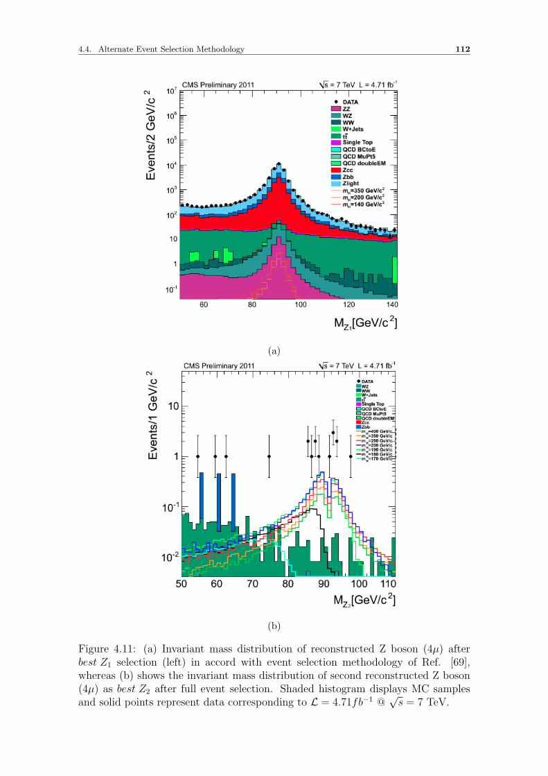
4.4. Alternate Event Selection Methodology 112
(a)
(b)
Figure 4.11: (a) Invariant mass distribution of reconstructed Z boson (4µ) afterbest Z1 selection (left) in accord with event selection methodology of Ref. [69],whereas (b) shows the invariant mass distribution of second reconstructed Z boson(4µ) as best Z2 after full event selection. Shaded histogram displays MC samplesand solid points represent data corresponding to L = 4.71fb−1 @
√s = 7 TeV.

4.4. Alternate Event Selection Methodology 113
4.4.1 Skimming
A preliminary selection of events, referred to as a skim, is designed to reduce the data
set to a manageable size while preserving high signal selection efficiency. The skim
is common to all 4` channels, requires the HLT selection described in the previous
section, the requirement of at least one same flavor di-lepton candidate selected with
the following criteria on the component leptons:
• leptons of opposite charge, reconstructed with either the electron basic track-
supercluster objects, global muon objects, or tracker muon objects.
• electrons and muons should be within the geometrical acceptance of |ηe| < 2.5,
|ηµ| < 2.4 with peT > 7 GeV/c, pµT > 5 GeV/c.
• invariant mass of at least one di-lepton pair (made from OS-SF leptons) should
be greater than 40 GeV/c2.
4.4.2 Event selection
The leptons should be loosely isolated lepton candidates. A lepton is defined as
loosely isolated if the sum∑
i piT,track of the transverse momentum of the tracks
divided by p`T is less than 0.7. The tracks are lying in a cone of radius ∆R =√∆η2 + ∆φ2 < 0.3 around the lepton ` with axis along the lepton candidate di-
rection, excluding a central inner ‘veto’ region of width ∆η < 0.015 (electron) or
∆R < 0.015 (muon), which contains the lepton candidate track footprint. The ∆φ
is the difference between azimuthal angles of two leptons (i.e. φ1 and φ2), which
are lying outside inner veto of 0.015 and within ∆R < 0.3. The lepton isolation
efficiency for identified leptons within this very loose isolation is found to be greater
than 99%. Once an event satisfies the above mentioned quality criterion, the 4
lepton signal selection strategy implemented as given below:
• Each 4` candidate in an event is treated individually by checking the quality
parameters of its daughters.
• 4` daughters should have plT1 > 20, plT2 >10, plT,3,4 > 7 GeV/c (5 GeV/c) for
electrons (muons).
• Baseline: The mass cuts over Z boson have been lowered to make the anal-
ysis strategy compatible to low mass Higgs searches. One Z should have mZ
between 50 GeV/c2 to 120 GeV/c2 and mZ for second Z should be within 12
GeV/c2 to 120 GeV/c2.

4.4. Alternate Event Selection Methodology 114
• Intermediate: This region is compatible to Higgs searches in intermediate
mass range, where invariant mass of one Z should lie between 60 GeV/c2 to
120 GeV/c2 and mZ for second Z should be within 20 GeV/c2 to 120 GeV/c2.
• High mass: This class is used for ZZ cross-section measurement as it’s suit-
able for high mass Higgs searches, where possibility increases to get both on
mass shell Z boson. The corresponding selection range over invariant mass of
Z for both Z bosons is 60 < mZ < 120 GeV/c2.
• significance of the impact parameter to the event vertex, SIP3D, is required to
satisfy SIP3D = |IP|σIP
< 4 for each lepton.
• The combined relative isolation should be < 0.35 for each lepton.
• The invariant mass of four lepton candidate (m4` ) should be greater than 100
GeV/c2.
• In case of more than one 4 lepton candidates, select one having at least one Z
particle whose mass is close to real Z mass.
4.4.3 Results
The expected improvement is shown in Fig. 4.12, which represents the invariant
mass distributions of mZ1, mZ2, m4e and m4µ. It is observed that asymmetry over Z
mass peak in case of mZ2 is resolved and invariant mass spectrum of Z boson is well
reproduced by Data and MC for 4e and 4µ final states. All plots are obtained after
applying full selection criterion described above. The large error bars associated to
data points are caused by the less number of events surviving full selection.
The signal selection efficiency for each step of selection is shown in Fig. 4.13a
and 4.13b for 4e and 4µ final states respectively. The X-axis represents Higgs signal
selection efficiency and simulated Higgs masses (mH) are represented along Y-axis.
The signal selection efficiency is calculated as follows:
ε =AeventsBevents
(4.10)
where:
• ε is the Higgs signal selection efficiency.
• Aevents represents total number of events satisfying the |η| < 2.5 (2.4) for
electrons (muons) and pT > 7 GeV/c (5 GeV/c) for electrons (muons).
• Bevents is the total number of events surviving corresponding selection cut.
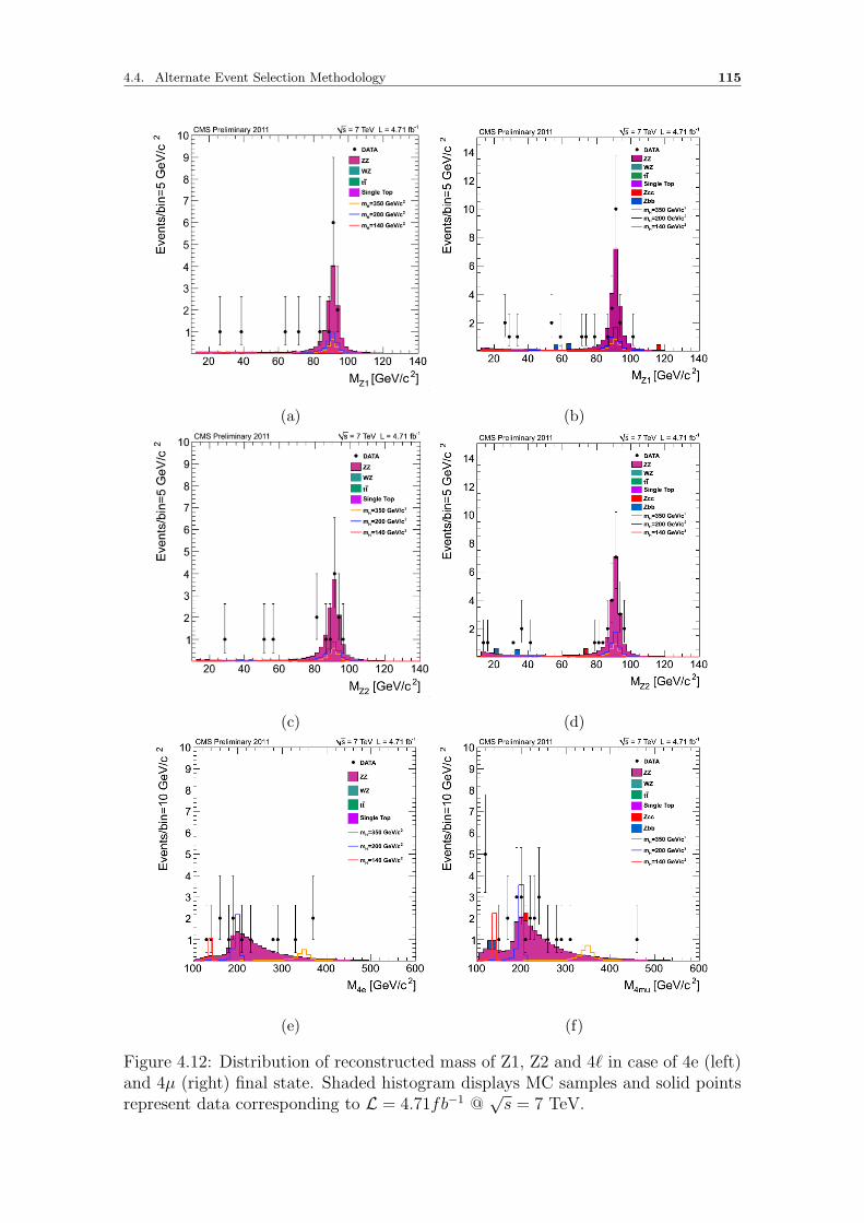
4.4. Alternate Event Selection Methodology 115
(a) (b)
(c) (d)
(e) (f)
Figure 4.12: Distribution of reconstructed mass of Z1, Z2 and 4` in case of 4e (left)and 4µ (right) final state. Shaded histogram displays MC samples and solid pointsrepresent data corresponding to L = 4.71fb−1 @
√s = 7 TeV.

4.4. Alternate Event Selection Methodology 116
The overall small signal selection efficiency for lower Higgs masses can be under-
stood from Fig. 3.6 and 3.8a, which shows that analysis cuts like m4` > 100 GeV/c2
and pT cut over leptons can decrease the number of signal events considerably along
with background events after full selection.
Moreover, it is observed that selection efficiency for Higgs signal is increased
by 4% (10%) in case of 4e (4mu) for Higgs mass 120 GeV/c2 as compared to Ref.
[69]. This increase in signal selection efficiency is followed by relative increase in
background contribution as well. The cut wise status of event yield of contributing
samples has been shown in Tab. 4.9 and 4.10 for 4e and 4mu final states.
(a) (b)
Figure 4.13: Signal selection efficiencies for Higgs masses, 4e (a) and 4µ (b). Shadedhistogram displays MC samples and solid points represent data corresponding toL = 4.71fb−1 @
√s = 7 TeV.

4.4. Alternate Event Selection Methodology 117
Table 4.9: The cut wise status of event yields of contributing samples in 4µ finalstate
Sample Skimm 4l SIP Riso Baseline Intermediate High mass
QCD 769631 0 0 0 0 0 0tt 11013 11.16 1.46 0.04 0.04 0.03 0.008Z+ jets 1.5e+06 0.4 0 0 0 0 0Zbb 124526 25.4 5.2 0.8 0.8 0.4 0Zcc 578439 0.8 0.4 0.4 0.4 0.4 0.4WZ 642.04 0.16 0.08 0.025 0.025 0.023 0.005ZZ 197.94 29.36 24.6 22.9 22.9 21.02 17.61H 200 32.63 5.34 5.12 4.74 4.74 4.72 4.37Total 2975069 67.28 31.73 24.19 24.19 21.87 18.02
Data 3312214 168 36 27 27 24 15
Table 4.10: The cut wise status of event yields of contributing samples in 4e finalstate
Sample Skimm 4l SIP Riso Baseline Intermediate High mass
QCD 48614 0 0 0 0 0 0tt 6167 2.82 0.69 0.016 0.016 0.008 0.008Z+ jets 1.3 e+06 2.38 0.8 0 0 0 0Zbb 108234 3.17 0 0 0 0 0Zcc 511890 2.38 0.4 0 0 0 0WZ 578.6 0.28 0.18 0.069 0.069 0.061 0.02ZZ 174.3 18.99 16.02 14.36 14.36 13.76 11.9H 200 28.8 4.0 3.7 3.2 3.2 3.14 2.87Total 1.9e+06 30.04 18.08 14.44 14.44 13.83 11.93
Data 2146946 39 19 14 14 14 9

4.5. H→ ZZ∗ → 4` analysis by Bayesian Approach 118
4.5 H→ ZZ∗ → 4` analysis by Bayesian Approach
The search of the SM Higgs boson in the H→ ZZ∗ → 4` decay channel is also per-
formed by using a multivariate technique [77] known as Bayesian neural networks
(BNNs) [78]. Signal and background discriminants are derived and the results are
compared to the baseline cut-based method. A detailed treatment of H→ ZZ∗ → 4`
decay channel via BNN approach have been reported in Refs. [79], [80].
The analysis have been performed over proton-proton collision data recorded by
the CMS detector at the LHC, corresponding to integrated luminosities of 4.71 fb−1
@√s = 7 TeV (2010 & 2011) and 5.26 fb−1 @
√s = 8 TeV (2012).
A “multivariate discriminant” function D(x) is used to classify objects charac-
terized by a vector of properties x. In our case, we use D(x) to classify events as
signal s(x) or background b(x) with minimum classification error 2. The consistently
Bayesian method uses a binned likelihood constructed from a multivariate discrimi-
nant D(x) and a 4` mass distribution created from a comprehensive set of simulated
events for signal and background.
I have estimated the reducible background contribution in signal region by using
methodology explained in previous sections. The estimated values of background are
used for training of the BNN events to get input histogram for background samples,
which are used to calculate the binned likelihood D(x) vs. m4`. The 4µ, 4e and 2e2µ
decay channels were trained separately.
2In principle, the discriminant should be chosen to minimize directly the quantity of interest.Experience suggests, however, that a discriminant that minimizes classification error performs wellin practice.

Chapter 5
Results and Statistical
Interpretation
The first half of current chapter will reveal the background estimation results in
respective control regions and relative uncertainties over their measurements will be
briefly discussed. While the second half will cover results obtained by using esti-
mated values of corresponding backgrounds in signal region i.e. about mass mea-
surements and statistical results.
5.1 ZZ Continuum
The total number of events in Higgs signal region and relative uncertainties from
ZZ∗ → 4` have been estimated from Monte Carlo simulation. The corresponding
event yield and uncertainties are described in following Tab. 5.1.
Table 5.1: Number of ZZ background events expected and relative uncertainties inthe signal region estimated from Monte Carlo simulation, for 5.1 fb−1 at 7 TeV and12.21 fb−1 at 8 TeV data. Uncertainty on the yields due to QCD scale and the choiceof parton distribution functions is also reported. Only the Monte Carlo statisticaluncertainty is shown.
(a) 7 TeV
qq NZZ→4e 13.3 ± 0.06NZZ→4µ 20.77 ± 0.08NZZ→2e2µ 31.8 ± 0.3
gg NZZ→4e 0.91 ± 0.01NZZ→4µ 1.28 ± 0.01NZZ→2e2µ 2.15 ± 0.08
(b) 8 TeV
qq NZZ→4e 36.9 ± 0.2NZZ→4µ 56.2 ± 0.2NZZ→2e2µ 89.8 ± 0.6
gg NZZ→4e 2.22 ± 0.01NZZ→4µ 3.06 ± 0.02NZZ→2e2µ 6.51 ± 0.20
119

5.2. Reducible and Instrumental Backgrounds 120
5.1.1 Uncertainties in ZZ measurement
The theoretical uncertainties have been calculated over event yield as a function
of m4` in Ref. [62]. These are briefly discussed here for completeness. PDF+αs
and QCD scale uncertainties for pp → ZZ → 4` at NLO and gg → ZZ → 4` are
evaluated using MCFM [75]. The 2e2µ final state has been used with following
fiducial cuts for leptons:
• electrons should have pT > 7 GeV/c and |η| < 2.5.
• muon’s pT should be greater than 5 GeV/c and |η| < 2.4.
• invariant mass of di-electron and di-muon pairs must be greater than 12
GeV/c2.
The cross sections are calculated inclusively in the number of jets found at NLO.
The uncertainties are assessed both for 7 TeV and 8 TeV and assumed to be 100%
correlated. The PDF+αs and QCD scale uncertainties are treated as uncorrelated.
The shape uncertainties in m4` distribution imply the knowledge of correlations
between possible event yield variations at different m4` points. For simplicity, 100%
correlation is assumed between errors across the entire m4` mass range. With O(70)
observed ZZ → 4` events, the statistical error is about 12%, which is larger than
the current theoretical error of O(5%).
5.2 Reducible and Instrumental Backgrounds
The number of events along with corresponding expected event yield from Z+X and
the relative systematic and statistical errors in the signal region in a mass range
from m1 = 100 GeV/c2 to m2 = 600 GeV/c2 for the baseline selections are listed in
Tab. 5.2.
The statistical error quoted represents the number of events in the control region,
while the systematics one is extracted by varying the fake rates by ±1 sigma and
inflated by 10% according to the WZ underestimation.
5.2.1 Relative Uncertainties
The assessment of statistical and systematic uncertainties over reducible background
prediction method and various sources of uncertainties are discussed below:

5.2. Reducible and Instrumental Backgrounds 121
Table 5.2: The number of events from Z+X expected and the relative systematicsand statistical errors in the signal region in a mass range from m1 = 100 GeV/c2 tom2 = 600 GeV/c2.
Analysis over 7 TeV data
Sample Baseline (full range)
NZ→X→4e 1.7 ± 0.07 (4%) (stat., 649 events) ±0.85 (50%) (syst.)NZ→X→4µ 0.5 ± 0.06 (12%) (stat., 87 events)±0.25 (50%) (syst.)NZ→X→2µ2e 2.0 ± 0.06 (3%) (stat., 839 events)±1.0 (50%) (syst.)
Analysis over 8 TeV data
Sample Baseline (full range)
NZ→X→4e 5.5 ± 0.1 (2%) (stat., 1932 events)±2.75 (50%) (syst.)NZ→X→4µ 1.6 ± 0.1 (6%) (stat., 204 events)±0.8 (50%) (syst.)NZ→X→2µ2e 7.9 ± 0.16 (2%) (stat., 2685 events)±3.95 (50%) (syst.)
• The dependance of fake ratios on the exact composition of background pro-
cesses in a region of interest is one of the main source of systematic uncertain-
ties of the method. The statistical uncertainty of 50% is assigned due to less
statistics in signal region.
• The current method can underestimate the reducible background containing
three real leptons and one jet faking lepton like WZ. While MC studies have
shown that the overall contribution of WZ to the total reducible background
is small (between 5 and 10%). The total reducible background estimated with
the Z+X method may therefore be underestimated by a small amount (about
7%). This is taken into account by increasing the systematic of the Z+X
method by 10%.
• The compositions of reducible background processes (DY , tt, WZ, Zγ(∗))
in the region where fake ratios are measure and applied, are typically not the
same. The dominating statistical uncertainty is driven by the number of events
in the control region and is typically in the range of 5-10%.
• The functional form for the invariant mass (m4`) shape that is used to ex-
trapolate from the full range of m4` to the range of interest is another source
of the systematic uncertainty. The respective differences between the shapes
of predicted background distributions for all three channels have been exam-
ined in order to estimate it. The envelope of differences between these shapes
of distributions is used as a measure of the uncertainty of the shape. The
uncertainty is estimated to be up to 10 - 15%.

5.3. The H→ ZZ∗ → 4` Phase Space 122
5.3 The H→ ZZ∗ → 4` Phase Space
The number of candidates observed in 2011 and 2012 data are reported in Tab.
5.3 and 5.4 for the baseline selection in accord with the three final states. These
numbers are accompanied by estimated background contributions in the signal re-
gion. The reconstructed four-lepton invariant mass distribution is shown in Fig.
5.1 for the full dataset, where different mass ranges are shown, including the mass
below 100 GeV/c2 (not used for analysis). The SM background distributions are
obtained by combining the rate normalization from data-driven methods and knowl-
edge on shapes taken from the MC samples. Fig. 5.2 is showing the invariant mass
distribution of reconstructed Z1 and Z2.
The statistical procedure followed to derive upper limits on the SM Higgs boson
cross section times branching ratio is the so-called CLs method, described in Ref.
[71]. The expected and observed upper limits at 95% confidence level on the signal
strength modifier µ = σ/σSM are shown in Fig. 5.3. In other words, the plot shows
the factor by which the SM Higgs boson cross section times branching ratio must be
scaled to be excluded at 95% CL, as a function of the Higgs mass. The dashed line
has been obtained by tossing toy Monte Carlo pseudo experiments, whereas the solid
line shows the results obtained from real data. The green and yellow bands indicate
the µ ranges in which an additional measurement would lie with a probability of
68% and 95%, respectively. An upper limit at 95% confidence level exclude the
ranges 113 - 116 GeV/c2 and 129 - 720 GeV/c2 while the expected exclusion range
for the standard model Higgs boson is 118 - 670 GeV/c2.
The compatibility of the observed excesses of data events with the background-
only hypothesis can be quantified by the p-value. The p-value is the probability
of observing an upwards fluctuation of the background event yield at least as large
as the one measured in data. It is estimated by tossing a large number of toy MC
pseudo-datasets. Its trend as a function of the SM Higgs boson mass is plotted
in Fig. 5.4. A local significance above the expected background of 4.5 standard
deviations is observed at mH ≈ 126 GeV/c2.

5.3. The H→ ZZ∗ → 4` Phase Space 123
Table 5.3: The number of event candidates observed in 2011 data at L = 5.05 fb−1,compared to the mean expected background and signal rates for each final state for100 < m4` < 1000 GeV/c2. For the Z + X background, the estimations are basedon data.
Channel 4e 4µ 2e2µ
Z + X 1.88+2.45−1.13 0.99+1.49
−0.6 2.97+2.97−1.49
ZZ background 15.06 ±1.71 22.58 ±2.23 35.66 ±3.64
All background expected 16.94+2.99−2.05 23.58+2.68
−2.31 38.63+4.7−3.93
mH = 125 GeV 0.65 ±0.1 1.2 ±0.13 1.54 ±0.18mH = 126 GeV 0.72 ±0.11 1.3 ±0.14 1.71 ±0.2mH = 200 GeV 4.12 ±0.48 5.86 ±0.59 9.84 ±1.02mH = 350 GeV 2.34 ±0.28 3.21 ±0.34 5.59 ±0.61mH = 500 GeV 0.81 ±0.1 1.08 ±0.12 1.89 ±0.21Observed 14 20 43
Table 5.4: The number of event candidates observed in 2012 data at L = 12.21 fb−1,compared to the mean expected background and signal rates for each final state for100 < m4` < 1000 GeV/c2. For the Z + X background, the estimations are basedon data.
Channel 4e 4µ 2e2µ
Z+X 4.46+7.58−3.12 2.08+2.29
−1.04 7.04+11.26−4.22
ZZ background 40.2 ±4.7 60.14 ±6.66 98.35 ±10.71
All background expected 44.66+8.92−5.64 62.22+7.04
−6.74 105.39+15.54−11.51
mH = 125 GeV 1.8 ±0.25 3.47 ±0.41 4.52 ±0.54mH = 126 GeV 1.99 ±0.28 3.79 ±0.44 4.99 ±0.6mH = 200 GeV 12.68 ±1.52 17.82 ±2.02 30.4 ±3.38mH = 350 GeV 7.66 ±0.94 10.27 ±1.19 18.2 ±2.07mH = 500 GeV 2.8 ±0.35 3.68 ±0.43 6.51 ±0.75Observed 45 75 119

5.3. The H→ ZZ∗ → 4` Phase Space 124
(a) (b)
Figure 5.1: Distribution of the four-lepton reconstructed mass, (a) represents lowmass region and (b) is displaying full mass range considered in the analysis. Regionm4l < 100 GeV/c2 is shown but not used in analysis. The sample correspond to anintegrated luminosity of L = 5.1 fb−1 of 2011 data and L = 12.21 fb−1 of 2012 data.
(a) (b)
Figure 5.2: Fig. (a) and (b) are showing invariant mass distributions of Z1 and Z2respectively. The sample correspond to an integrated luminosity of L = 5.1 fb−1 of2011 data and L = 12.21 fb−1 of 2012 data.

5.3. The H→ ZZ∗ → 4` Phase Space 125
(a)
(b)
Figure 5.3: Observed and expected 95% CL upper limit on the ratio of the produc-tion cross section to the SM expectation with the 2D fit. 2011 and 2012 data-samplesare used. The 68% and 95% ranges of expectation for the background-only modelare also shown with green and yellow bands, respectively. (a) represents lower massrange only and (b) shows full mass range.

5.3. The H→ ZZ∗ → 4` Phase Space 126
(a)
(b)
Figure 5.4: Significance of the local fluctuations with respect to the standard modelexpectation as a function of the Higgs boson mass for an integrated luminosity of5.1 fb−1 at 7 TeV and 12.21 fb−1 at 8 TeV in the low mass range (110 - 180 GeV/c2)in (a) and in the mass range (110 -1000 GeV/c2) in (b). Dashed line shows meanexpected significance of the SM Higgs signal for a given mass hypothesis.

5.4. ZZ Cross Section Measurement 127
5.4 ZZ Cross Section Measurement
The initial event selection strategy for ZZ cross section measurement is same as
described in Sec. 4.2 but events are constrained to follow mass cuts over Z1, Z2 and
m4` in accord with High-mass phase space only to get both on mass shell Z bosons.
The background contributions extrapolated in signal region for high mass region
contributed in cross section measurement as well, which is reported individually for
7 TeV and 8 TeV in Refs. [81] and [82] respectively. The measured values of ZZ
cross section with√s = 7 TeV & 8 TeV data are reported as:
• σ(pp→ ZZ) = 6.24+0.86−0.80(stat)+0.41
−0.32(syst.)± 0.14(lumi.) pb at 7 TeV.
• σ(pp→ ZZ) = 8.4± 1.0(stat.)± 0.7(syst.)± 0.4(lumi.) pb at 8 TeV.

5.4. ZZ Cross Section Measurement 128

Conclusions
The search of the SM Higgs boson has to encounter with various SM and electroweak
background processes that have similar final states as those of the signal. On the
way to the SM Higgs boson search in H→ ZZ∗ → 4` decay channel, the current
thesis have reported results from analysis of the background-like real data events in
accord with H→ ZZ∗ → 4` decay mode. The contribution of all SM and electroweak
background processes, contributing in signal phase space have been estimated. In
parallel, the proper understanding of the Higgs signal is equally important to com-
prehend the status of various background events in signal phase space, which leads
to the methodological developments for their precise evaluation in signal region.
The analysis have been presented over proton-proton collision data recorded by
the CMS detector at the LHC, corresponding to integrated luminosities of 5.05 fb−1
@√s = 7 TeV (2011) and 12.21 fb−1 @
√s = 8 TeV (2012) to perform cut based
analysis in two different phase spaces i.e. background and Higgs signal.
The major part of research activities was devoted to examine the feasible de-
velopments of new techniques for background measurements and to improve the
efficiency of existing ones. The multiple ways were checked and studied for back-
ground estimation and most efficient techniques are reported in current work.
The very initial tenure of my analysis studies was devoted to comprehend the
signatures of predominant source of backgrounds giving 4 leptons as final state.
These were categorized as irreducible ZZ continuum, reducible backgrounds (Zbb,
Zcc & tt) and instrumental backgrounds (Z+jets or WZ+jet(s)) in accord with
their experimental signatures. The preliminary analyses of all these background
processes including Higgs signal samples have been performed over MC generator
level samples and contributed to comprehend the topologies of individual final states
by understanding the signatures of the relevant decays. The important kinematic
distributions (m4l, m``, pT of leptons etc.) obtained at MC level have shown the
inherent challenges to get a clear Higgs signal signature in low mass range. It dis-
plays the impulse to development of effective background estimation methodologies
by paying particular attention to low mass Higgs searches and contributed in the de-
129

velopment of event selection strategy for background and Higgs signal phase spaces.
The present work have contributed in the development and improvement of the
techniques to reconstruct H→ ZZ∗ → 4` final sates in accord with individual lepton
flavor (4e, 4µ, 2e2µ), by keeping higher efficiency to select Higgs signal.
The irreducible ZZ continuum have been measured from MC to get its estimate
in Higgs signal phase space. On the other hand, to cop with low MC statistics
problem in case of instrumental (Z + light jets, WZ + jets) & reducible (Zbb, Zcc,
tt) backgrounds, an inclusive approach has been accomplished for their measurement
directly from data by applying fake rate probabilities over leptons to be misidentified
by jets. The event rates measured in the background control region are extrapolated
to the signal region to evaluate their contribution in Higgs signal phase space.
In addition, the feasible improvements in the H→ ZZ∗ → 4` event selection
methodology to increase the Higgs signal selection efficiency has been examined.
The studies presented in this thesis over background estimations have contributed
in below mentioned research:
• The combined results at√s = 7 TeV & 8 TeV data in context of H→ ZZ∗ → 4`
analysis have resulted in an observation of a new boson with a local signifi-
cance above the expected background of 4.5 standard deviations as shown in
Ref. [76]. It could be the SM Higgs boson but it’s not yet confirmed. A mea-
surement of its mass gives 126.2 ± 0.6 (stat) ± 0.2 (syst) GeV/c2. No other
significant excess is found, and upper limits at 95% confidence level exclude
the mass ranges 113 - 116 GeV/c2 and 129 - 720 GeV/c2 while the expected
exclusion range for the standard model Higgs boson is 118 - 670 GeV/c2.
• The ZZ cross section measurement at√s = 7 TeV & 8 TeV data.
130

Bibliography
[1] ALEPH, DELPHI, L3, OPAL Collaborations, and LEP Working Group for
Higgs Boson Searches, “Search for the standard model Higgs boson at LEP ”,
Phys. Lett. B, 565 (2003) 61.
[2] The Tevatron New-Phenomena and Higgs Working Group, for the CDF and
D0 Collaborations, “Combined CDF and D0 Search for Standard Model Higgs
Boson Production with up to 10 fb−1 of Data”, FERMILAB-CONF-12-065-E,
CDF Note 10806, D0 Note 6303.
[3] K. Nakamura et al., “Review of particle physics”, J.Phys.G,vol. G37, p. 075021,
2010.
[4] G. Bertone, D. Hooper, and J. Silk, “Particle dark matter: Evidence, candidates
and constraints”, Phys.Rept., vol. 405, pp. 279-390, 2005.
[5] N. Jarosik, C. Bennett, J. Dunkley, B. Gold, M. Greason, et al., “Seven-Year
Wilkinson Microwave Anisotropy Probe (WMAP) Observations: Sky Maps,
Systematic Errors, and Basic Results,”. Astrophys.J.Suppl., vol. 192, p. 14,
2011.
[6] A. D. Martin F. Halzen. “Quarks Leptons: An Introductory Course in Modern
ParticlePhysics”. Wiley, 1984.
[7] D. H. Perkins. “Introduction To High Energy Physics”. Cambridge University
Press, 2000.
[8] S. Dawson, “Introduction to Electroweak Symmetry Breaking”, hep-
ph/9901280.
[9] S. Chatrchyan et al. [CMS Collaboration], “Observation of Z decays to four
leptons with the CMS detector at the LHC”, arXiv:1210.3844, [hep-ex].
[10] ATLAS Collaboration, “An update to the combined search for the Standard
Model Higgs boson with the ATLAS detector at the LHC using up to 4.9 fb−1
131

of pp collision data at√s = 7 TeV”, ATLAS Conference Report, ATLAS-
CONF-2012-019, (2012).
[11] CMS searchesCollaboration, “ Combination of SM, SM4, FP Higgs boson”,
CMS Physics Analysis Summary, CMS-PAS-HIG-12-008, (2012).
[12] LHC Higgs Cross Section Working Group, S. Dittmaier, C. Mariotti, G. Pas-
sarino, and R. Tanaka (Eds.), “Handbook of LHC Higgs Cross Sections: 1.
Inclusive Observables”, CERN-2011-002, CERN, Geneva, 2011.
[13] The LHC Study Group Collaboration. “LHC-the Large Hadron Collider accel-
erator project”. Technical report, CERN-AC-93-03, 2003.
[14] The LHC Study Group Collaboration. “LHC-the Large Hadron Collider con-
ceptual design”. Technical report, CERN-AC-95-05, 2005.
[15] L. Evans, P. Bryant [LHC Collaboration]. “LHC - Machine“. JINST, 3, 2008.
[16] K Nakamura and Particle Data Group, “Review of particle physics.”, of Physics
G: Nuclear and Particle Physics, 37(7A):075021, 2010.
[17] Roger Eckhardt. Stan Ulam, John Von Neumann, and the Monte Carlo method.
Los Alamos Science, Special Issue 15, 15:131-137, 1987.
[18] M.A. Dobbs et al., “Les houches guidebook to monte carlo generators for
hadron collider physics”, hep-ph/0403045, 2004.
[19] T. Sjostrand, S. Mrenna, and P. Skands, “PYTHIA 6.4 Physics and Manual”,
JHEP, 05(026), 2006.
[20] S. Alioli et al., “A general framework for implementing nlo calculations in
shower monte carlo programs: the powheg box”, JHEP, 1006:043, 2010.
[21] T. Binoth, N. Kauer, and P. Mertsch. “Gluon-induced QCD corrections to
pp→ ` ¯ ′ ¯′”, 2008.
[22] The Geant4 Collaboration, “GEANT-Detector Description and Simulation
Tool, http://geant4.web.cern.ch/geant4/..
[23] J. Alwall et al., “MadGraph/MadEvent v4: The New Web Generation”, JHEP
09 (2007) 028.
[24] H.-L. Lai et al., “Uncertainty induced by QCD coupling in the CTEQ global
analysis of parton distributions”, Phys. Rev. D, 82 (2010) 054021.
132

[25] M. Mohammadi Najafabadi, “Single Top production at LHC”, arXiv:hep-
ex/0605034, 2006.
[26] Pierini, M., “talk at the Joint PVT/PO Meeting”,
https://twiki.cern.ch/twiki/bin/viewauth/CMS/PdwgMain, 2011.
[27] C. Mariotti et al. LHC Higgs Cross Section Working Group, S. Dittmaier.
“Handbook of LHC Higgs Cross Sections:1. Inclusive Observables”. Technical
report, CERN, Geneva., 2011.
[28] CMS Collaboration, “ MUO-10-004: Performance of CMS muon reconstruction
in pp collision events at√s = 7 TeV”, Technical report, In preparation to JINST
(2010).
[29] G. Daskalakis et al., “Measuring Electron Efficiencies at CMS with Early Data”,
CMS Analysis Note 2007/019, 2007.
[30] Hung-Liang Lai et al. “New parton distributions for collider physics“. Phys.
Rev., D82, 2010.
[31] R. D. Ball, L. Del Debbio, S. Forte, A. Guffanti, J. I. Latorre, J. Rojo and M.
Ubiali, “A first unbiased global NLO determination of parton distributions and
their uncertainties”, Nucl. Phys B (2010), no. 838, 136.
[32] A. D. Martin, W. J. Stirling, R. S. Thorne and G. Watt, “Parton distributions
for the LHC”, Eur. Phys. J C, (2009), no. 63, 189.
[33] C. Anastasiou, R. Boughezal, and F. Petriello, “Mixed QCD-electroweak cor-
rections to Higgs boson production in gluon fusion”, JHEP, 04 (2009) 003.
[34] D. de Florian and M. Grazzini, “Higgs production through gluon fusion: up-
dated cross sections at the Tevatron and the LHC”, Phys. Lett. B 674 (2009)
291.
[35] S. Dawson, “Radiative corrections to Higgs boson production”, Nucl. Phys. B,
359 (1991) 283.
[36] M. Spira et al., “Higgs boson production at the LHC”, Nucl. Phys. B, 453
(1995) 17.
[37] R. V. Harlander and W. B. Kilgore, “Next-to-next-to-leading order Higgs pro-
duction at hadron colliders”, Phys. Rev. Lett., 88 (2002) 201801.
133

[38] C. Anastasiou and K. Melnikov, “Higgs boson production at hadron colliders
in NNLO QCD”, Nucl. Phys. B, 646 (2002) 220.
[39] V. Ravindran, J. Smith, and W. L. van Neerven, “NNLO corrections to the
total cross section for Higgs boson production in hadron-hadron collisions”,
Nucl. Phys. B, 665 (2003) 325.
[40] Y. Gao, A. V. Gritsan, Z. Guo et al., “Spin determination of single-produced
resonances at hadron colliders”, Phys.Rev. D81 (2010) 075022.
[41] S. Catani et al., “Soft-gluon resummation for Higgs boson production at hadron
colliders”, JHEP, 07 (2003) 028.
[42] S. Actis et al., “NLO Electroweak Corrections to Higgs Boson Production at
Hadron Colliders”, Phys. Lett. B, 670 (2008) 12.
[43] M. Ciccolini, A. Denner, and S. Dittmaier, “Strong and electroweak corrections
to the production of Higgs + 2-jets via weak interactions at the LHC”, Phys.
Rev. Lett., 99 (2007) 161803.
[44] M. Ciccolini, A. Denner, and S. Dittmaier, “Electroweak and QCD corrections
to Higgs production via vector-boson fusion at the LHC”, Phys. Rev. D, 77
(2008) 013002.
[45] T. Figy, C. Oleari, and D. Zeppenfeld, “Next-to-leading order jet distributions
for Higgs boson production via weak-boson fusion”, Phys. Rev. D, 68 (2003)
073005.
[46] K. Arnold et al., “VBFNLO: A parton level Monte Carlo for processes with
electroweak bosons”, Comput. Phys. Commun., 180 (2009) 1661.
[47] P. Bolzoni et al., “Higgs production via vector-boson fusion at NNLO in QCD”,
Phys. Rev. Lett., 105 (2010) 011801.
[48] A. Bredenstein et al., “Precise predictions for the Higgs-boson decay
H→WW/ZZ→4 leptons”, Phys. Rev. D 74 (2006) 013004.
[49] S.Dittmaier et al. A. Bredenstein, A. Denner. “Radiative corrections to
the semileptonic and hadronic Higgs-boson decays H→WW/ZZ→4 fermions”.
JHEP, 0702(080), 2007.
[50] A. Djouadi, J. Kalinowski, M. Muhlleitner et al. “An update of the program
HDECAY“. In The Les Houches 2009 workshop on TeV colliders:The tools and
Monte Carlo working group summary report, 2010.
134

[51] G. Bozzi, S. Catani, D. de Florian et al., “Transverse-momentum resummation
and the spectrum of the Higgs boson at the LHC”, Nucl. Phys. B 737 (2006)
73.
[52] I. Pulljak et al. A. Denner, S. Heinemeyer. “Standard Model Higgs-Boson
Branching Ratios with Uncertainties”. Eur. Phys. J., C71(1753), 2011.
[53] S. Actis, G.Passarino, C. Sturm et al. “NNLO Computational Techniques: the
Cases H → γγ and H → gg“. Nucl. Phys., B811:182–273, 2009.
[54] S. Baffioni et al. “Search strategy for the Higgs boson in the ZZ∗ decay channel
with the CMS experiment”, CMS-AN, 2010/237, 2008.
[55] M. Cacciari, S. Frixione, M. Mangano et al., “Updated predictions for the total
production crosssections of top and of heavier quark pairs at the Tevatron and
at the LHC”.
[56] W. Adam, S. Baffioni, F. Beaudette et al. “Electron Reconstruction in CMS“.
CMS AN-2009/164, November 2009.
[57] CMS Collaboration, “ Electron reconstruction and identification at√s = 7 7
TeV”, CMS Physics Analysis Summary, CMS-PAS-EGM-10-004 (2010).
[58] CMS Collaboration, “ Electron commissioning results at at√s = 7 TeV“, CMS
Detector Performance Summaries 2011/003 (2011).
[59] S. Baffioni et al, “ Electron Charge Determination Commissioning from 7 TeV
Data”, CMS-AN, 2010/468 (2010).
[60] M. Cacciari and G. P. Salam, “Pileup subtraction using jet areas”, Phys. Lett.
B659 (2008) 119-126.
[61] M. Cacciari, G. P. Salam, and G. Soyez, “The Catchment Area of Jets, JHEP
04 (2008) 005.
[62] CMS Collaboration, “Updated results on the new boson discovered in the
search for the standard model Higgs boson in the H → ZZ → 4l channel in pp
collisions at√s = 7 and 8 TeV”, CMS-AN, 2012/367 (2012).
[63] G. Abbiendi, N. Adam et al. “Muon Recostruction in the CMS Detector“. CMS
AN 2008/097, July 2009.
[64] K. Fruhwirth, “Application of Kalman filtering to track and vertex fitting”,
Nucl.Instrum.Meth. A, 262 (1987) 444.
135

[65] CMS Collaboration, “Performance of CMS muon reconstruction in cosmic-ray
events”, JINST, 5 (2010) T03022.
[66] CMS Collaboration, “CMS Physics Technical Design Report, volume I: Detec-
tor performance and software “, CERN/LHCC, 2006-001 (2006).
[67] CMS Collaboration, “Measurement of tracking efficiency”, CMS Physics Anal-
ysis Summary, CMS-PAS-TRK-10-002 (2010).
[68] A. Bodek and J. Han, “Improved Rochester Misalignment and Muon Scale Cor-
rections Extracted for 2011A, 2011B CMS Data”, CMS-AN 2012/298 (2012).
[69] CMS Collaboration, “Search for the standard model Higgs boson in the decay
channel H to ZZ to 4 leptons in pp collisions at√
(s) = 7 TeV”, Phys.Rev.Lett.,
108 (2012) 111804, February 2012.
[70] https://twiki.cern.ch/twiki/bin/view/CMS/MultivariateElectronIdentification
[71] A. L. Read. “Modified Frequentist analysis of search results (the CLs method)”.
Yellow Report 81, CERN-2000-005, 2000.
[72] S. Alekhin et al., “The PDF4LHC working group interim report, arXiv:hep-
ph/1101.0536..
[73] CMS Collaboration, “Commissioning of the particle-flow event reconstruction
with leptons from J/Psi and W decays at 7 TeV, CMS Physics Analysis Sum-
mary, CMS-PAS-PFT-10-003 (2010).
[74] CMS Collaboration, “Performance of CMS muon reconstruction in pp collisions
at√s = 7 TeV”, CMS PAS , MUO-10-002 (2010).
[75] K. Ellis C.W J. Campbell. “MCFM-Monte Carlo for FeMtobarn process”, 2011.
[76] CMS Collaboration, “Updated results on the new boson discovered in the
search for the standard model Higgs boson in the H → ZZ → 4l channel in pp
collisions at√s = 7 and 8 TeV”, CMS-PAS-HIG-12-041, November 2012.
[77] “https://twiki.cern.ch/twiki/bin/view/TMVA/WebHome”.
[78] “http://www.cs.toronto.edu/ radford/fbm.software.html”.
[79] J. Bochenek, P.C. Bhat, N. De Filippis, K.F. Johnson, H.B. Prosper, G. Singh,
S.Tentindo, “ Bayesian Search for a Higgs Boson in the Decay Channel H →ZZ → 4l”, CMS-AN-2012/334, September 2012.
136
[80] J. Bochenek, P.C. Bhat, D. Charles, N. De Filippis, K.F. Johnson, H.B. Prosper,
G.Singh, S. Tentindo, “Search for the Standard Model Higgs Boson in the Decay
Channel H → ZZ → 4l: a Bayesian Approach”, CMS-AN-2012/129, August
2012.
[81] CMS Collaboration, “Measurement of the ZZ production cross section and
search for anomalous couplings in 2l2l’ final states in pp collisions at√s = 7
TeV data”, CERN-PH-EP-2012-336,
[82] CMS Collaboration, “of ZZ production cross section in ZZ→ 2l2l’ decay channel
in pp collisions at√s = 8 TeV”, CMS-PAS-SMP-12-014, July 2012.
gluon fusion“.
137