universit at augsburg

Universitat Augsburg

Using Token Analysis to Transform

Graph-Oriented Process Models to

BPEL

Gotz, Roser, Lautenbacher & Bauer

Report 2008-08 Juni 2008

Institut fur InformatikD-86135 Augsburg

Copyright c© Mathias Gotz, Stephan Roser, Florian Lautenbacher & Bernhard BauerInstitut fur InformatikUniversitat AugsburgD–86135 Augsburg, Germanyhttp://www.Informatik.Uni-Augsburg.DE— all rights reserved —

In Business Process Management, graph-based models facilitate convenient process mod-elling. Current workflow engines are commonly based on mainly block-structured languages,such as WS-BPEL, that differ structurally and semantically from process graphs. Recentwork has accomplished elaborate mappings between both representations. Although mostmappings strongly depend on the segmentation of the graph-model into components, the nec-essary graph-decomposition itself is not described in these works. This article presents anapproach based on Token Analysis to automatically identify components. The technique en-ables simple integration of further improvements steps in the translation of process graphs toexecutable workflows and yields general results in graph-theory, that might also be of interestin related fields, such as workflow analysis for compilers and multi-threaded processors.

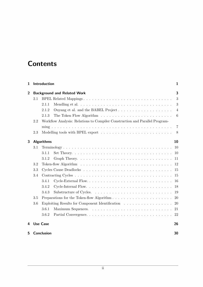
Contents

1 Introduction 1

2 Background and Related Work 3

2.1 BPEL Related Mappings . . . . . . . . . . . . . . . . . . . . . . . . . . . . . . . 32.1.1 Mendling et al. . . . . . . . . . . . . . . . . . . . . . . . . . . . . . . . . 32.1.2 Ouyang et al. and the BABEL Project . . . . . . . . . . . . . . . . . . . 42.1.3 The Token Flow Algorithm . . . . . . . . . . . . . . . . . . . . . . . . . 6

2.2 Workflow Analysis: Relations to Compiler Construction and Parallel Program-ming . . . . . . . . . . . . . . . . . . . . . . . . . . . . . . . . . . . . . . . . . . 7

2.3 Modelling tools with BPEL export . . . . . . . . . . . . . . . . . . . . . . . . . 8

3 Algorithms 10

3.1 Terminology . . . . . . . . . . . . . . . . . . . . . . . . . . . . . . . . . . . . . . 103.1.1 Set Theory. . . . . . . . . . . . . . . . . . . . . . . . . . . . . . . . . . . 103.1.2 Graph Theory. . . . . . . . . . . . . . . . . . . . . . . . . . . . . . . . . 11

3.2 Token-flow Algorithm . . . . . . . . . . . . . . . . . . . . . . . . . . . . . . . . 123.3 Cycles Cause Deadlocks . . . . . . . . . . . . . . . . . . . . . . . . . . . . . . . 153.4 Contracting Cycles . . . . . . . . . . . . . . . . . . . . . . . . . . . . . . . . . . 15

3.4.1 Cycle-External Flow. . . . . . . . . . . . . . . . . . . . . . . . . . . . . . 163.4.2 Cycle-Internal Flow. . . . . . . . . . . . . . . . . . . . . . . . . . . . . . 183.4.3 Substructure of Cycles. . . . . . . . . . . . . . . . . . . . . . . . . . . . 19

3.5 Preparations for the Token-flow Algorithm . . . . . . . . . . . . . . . . . . . . . 203.6 Exploiting Results for Component Identification . . . . . . . . . . . . . . . . . 20

3.6.1 Maximum Sequences. . . . . . . . . . . . . . . . . . . . . . . . . . . . . 213.6.2 Partial Convergence. . . . . . . . . . . . . . . . . . . . . . . . . . . . . . 22

4 Use Case 26

5 Conclusion 30

ii

1 Introduction

Graph-based models – commonly expressed in the Business Process Modelling Notation (BPMN,OMG (2006)) – enable intuitive modelling of processes: they are readily understandable with-out the need for learning abstract programming languages. A process is described as a state-transition system by vertex elements representing activities, events, gateways for decisions orparallel execution, and the connecting flow between them, represented by arcs. Implementa-tion concerns are covered in-depth in Jablonski & Bussler (1996). The expressive power ofgraph-based languages, however, also has some disadvantages. Graphs can be inconsistent orhave no defined meaning. The integrity of the model cannot be ensured on a syntactic level,as done in imperative programming, but requires further analysis.

Current workflow engines are very often based on imperative block-structured languages.The Business Process Execution Language for Web Services (WS-BPEL, OASIS (2003)) isa block-oriented language, but also includes graph-based control links. Language elements,like invoke, sequence or while, are composed in a tree-structure that differs essentially fromarbitrary, possibly cyclic graphs; while providing better control over semantics and misuseof syntax, the block structure requires experience in programming. This is not suitable forbusiness analysts and designers.

Recker & Mendling (2006) discusses the conceptual discrepancy between BPMN andBPEL. Originating from different backgrounds, the languages differ in their semantic ex-pressiveness because of the different paradigms in technical and business analysis. Second,BPMN is relevant at an early stage of BPM design, and BPEL in the late stage of execution.

To close the gap between ease of description and execution, recent work presents transfor-mation strategies. Mendling et al. (2006) and Ouyang, Dumas, ter Hofstede & van der Aalst(2006a) provide mappings from sub-graphs of BPMN models – henceforth called components1–to equivalent BPEL code. Automatic translation requires to determine all components andchose the best mapping strategies for them. For large scaled input, a structured and efficientapproach is needed.

OMG (2006) informally outlines in its BPMN specification a translation from BPMN toBPEL based on a technique called Token Analysis. Conceptual tokens flowing along the arcs

1In some fields of Compiler Theory and Parallel Programming, these subgraphs are referred to as hammockgraphs, see Sect. 2.2

1

1 Introduction

are used to identify the boundaries of structured components which are then mapped to BPELelements. The method depends on manual interaction for the identification of the structuredcomponents, so it is not suitable for an automatic export filter.

Existing techniques for automatic graph decomposition into components from relatedfields, in workflow analysis for compilers and multi-threaded processor design, are complexand not well adjusted to producing BPEL code. The objective of this work is to develop thebasic Token Analysis idea into a convenient segmentation algorithm, customised to businessprocess diagrams (BPDs, see OMG (2006)), that does not require human input.

This aims at building a bridge between the ideas proposed in the articles on Token Flowby OMG (2006) and the mapping routines by Ouyang, Dumas, ter Hofstede & van der Aalst(2006a). From the given informal description of the Token concept, we derive a machineexecutable algorithm. This involves investigating cyclic graph structures and their meaningto the analysis.

The overall result is an automatic and efficient algorithm for the segmentation of (process)graphs into components. The results further improve the translation procedure: we introducea new method called partial token convergence to detect additional components that onlybecome available through gateways splitting. This enhances the readability of the producedcode and is one major advantage of the algorithm introduced in this work, that is currentlynot supported by related techniques.

The benefits of the extended Token Analysis approach are:

• it works for arbitrary graphs,

• improvements in the translations procedure,

• enhanced readability of generated code.

Furthermore, our implementation of the Token Analysis algorithm, including automaticmapping to BPEL code, has proven that the algorithm successfully integrates in the overalltransformation. The developed Java framework can be used to enhance existing modellingtools with BPEL export. Furthermore, the algorithm and theoretical results convey insightsinto cyclic structures and their reduction to acyclic flow.

This article is structured as follows: Chapter 2 gives an overview of transformation strate-gies from graph to block structured models. The extended token analysis algorithm in Chap-ter 3 is presented as pseudo code and backed up by a proof-of-concept implementation, whichis applied to an example graph in Chapter 4. Finally, Chapter 5 concludes and discussesfuture work.

2

2 Background and Related Work

Recent work explores transformation strategies from graph structured process models to blockstructure. The mapping concepts involve a trade-off between readability of the output codeand completeness, that is the ability to transform arbitrary input models.

The mapping approaches described in 2.1.1 and 2.1.2 are the most specific to BPEL. 2.1.3introduces the Token Flow idea. Sect. 2.2 lists some alternate graph segmentations proceduresfrom compiler construction and parallel programming. Finally, 2.3 tries to capture the stateof BPEL export in current workflow modelling tools.

2.1 BPEL Related Mappings

The following mapping strategies are customised to produce BPEL code.

2.1.1 Mendling et al.

A process graph PG is represented in an EPC-like notation, consisting of a directed graphthat has special vertex types (called functions and connectors). Depending on the type,there are restrictions on input and output cardinalities, and some connector types have guardexpressions. For the transformation from PGs to BPEL we are concerned with here,

Mendling et al. (2006) uses an annotated graph, that is annotations at special vertices thatrefer to portions of successively translated BPEL code. In succeeding steps, subgraphs trans-late to BPEL. The article describes four different mapping strategies: Element-Preservationtranslates the whole graph to one BPEL <flow> activity. The graph must be acyclic be-cause of BPEL’s dead path elimination mechanism. Activities and start events map to BPELbasic activities, connectors (gateways) map to empty activities. Flow is uniformly mod-eled by control-links. This strategy produces less readable code and many undesired nodeswhich are reduced by Element-Minimization. Superfluous empty activities created by theformer method are replaced by direct links. Structure-Identification iteratively identifies andtranslates structured sub-graphs of the process graph to BPEL code and replaces sub-graphswith annotated vertices, carrying the corresponding translation. Structured sub-graphs have

3


a direct BPEL translation including sequences, pairs of connectors matching <flow> and<switch> activities and while and repeat loops. This method covers graphs that can beiteratively reduced to one annotated vertex. Finally, Structure-Maximization combines allstrategies by applying Structure-Identification until all possible structured activities havebeen translated, then ElementPreservation and Minimization for the remaining graph. Thisimproves readability while still working on a broader class of input graphs. The mappings aredescribed algorithmically, but in Structure-Maximization the best strategy has to be chosenmanually. Implementation details are not given, and many steps are described informally.The strategies do not work for arbitrary cyclic graphs.

2.1.2 Ouyang et al. and the BABEL Project

The BABEL group, that some of the authors of Ouyang, Dumas, ter Hofstede & van derAalst (2006a) belong to, is aimed at language heterogeneity and coherence, and has producedreference-implementations of their algorithms. The described techniques offer the most com-prehensive capabilities. van der Aalst & Lassen (2007) describes a semi-automatic pattern-based approach which is based on Petri nets. Ouyang, Dumas, Breutel & ter Hofstede (2006)instead shows a fully automatic approach based on event-condition-action rules which is ap-plied to BPMN as input producing BPEL code. The article describes event-action rules,using BPEL event handlers that represent unbounded parallelism by an unbounded numberof threads within a <scope> running simultaneously. <invoke> operations provide goto-likestructures. The strategy is further improved in Ouyang, Dumas, ter Hofstede & van derAalst (2006a) to a compact representation that can be directly implemented. Although themappings provide translations for arbitrary graphs, the produced code severely lacks read-ability. As a remedy, Ouyang, Dumas, ter Hofstede & van der Aalst (2006a) suggests thecombination with another translation type for well-structured sub-graphs on the same basisas Structure-Identification in Mendling et al. (2006). Sub-graphs having one single entry-pointand one exit-point are called components. The reduction of components to a single vertex iscalled folding and formalised in detail. Based on the decomposition of a process graph intocomponents, the article presents an incremental bottom-up overall translation.

The algorithm chooses the next component and transforms is using the best possible trans-formation strategy. Maximal sequence components are preferred to well-structured compo-nents. Unstructured (possibly cyclic) components are only transformed if no other optionis available using Event-Condition-Action-rules. This can enable the identification of newwell-structured components in the next iteration. The approach selects the best trade-offbetween readability and completeness for the two algorithms. Although the procedures aregiven algorithmically, no details are given on how to decompose a graph into its components.Ouyang et al. (2007) further extends the translation by mappings for components that are

4


not well-structured but can be translated without the use of event-handlers. Quasi-structuredpatterns describes a method to temporarily extend the graph structure by splitting gate-ways. This creates further components for pairs of gateways that make them match to one<switch>, <flow> or <pick> activity. (Ouyang et al. 2007, p.10) argues that the refinementof the guard conditions might become complicated and error-prone. In this thesis, we proposea solution on how the idea of gateway-splitting can be extended to work for XOR gateways.In Sect. 3.6.2 we show how to use Token Analysis to identify and create those components.Generalised flow-pattern translation uses one <flow> activity together with control links andworks for acyclic components that have no sub-components, only contain AND gateways andare safe and sound, that is guarantee not to cause any deadlocks during execution. First,several simple reduction steps are applied. Next, if sequence patterns or quasi-flow patternsexist, they are translated and folded remaining within the <flow>. If not, links through ANDgateways are replaced with direct control links inside the flow. Again, the process continuesiteratively, until everything has been translated.

The overall translation is similar as in Ouyang, Dumas, ter Hofstede & van der Aalst(2006a) but has an extended priority list:

1. maximal sequence components

2. well-structured components

3. quasi-structured components

4. generalised flow pattern

5. unstructured components

Furthermore, a technical report Ouyang, Dumas, ter Hofstede & van der Aalst (2006b)from the same group exists, in which another translation method is presented, called controllink-based translation algorithm. It is similar to the generalised flow-pattern, but can inaddition contain XOR gateways. Unfortunately, there exist some inconsistencies within thealgorithm.

It works for arbitrary cyclic sub-graphs, using event-handlers by event-action rule-basedtranslation. The work also includes a bottom-up procedure, called folding to automaticallytranslate process graphs. In succeeding steps the next component enabling the best trade-offis translated and folded to a single task object for the next iteration.

In Koehler & Hauser (2004), a control flow normalisation algorithm (described by Ammar-guellat (1992)) is used for process-graph to BPEL transformation. The graph is transformedinto a set of continuation equations consisting of a label, an instruction (invoke or if-branch) orgoto-like references to labels; they can be concatenated via a sequence operator. A set of rulesiteratively transforms the equations until only one remains. The remaining construct then has

5


a straightforward mapping to BPEL using <while>, <sequence> and <switch> activities andvariable assignments. Two issues within the transformation exist: first, the transformation isnot confluent, meaning a different order in rule applications result in output of differing, andsecond, non-reducible input models result in duplicate BPEL code fragments. Concerningconfluence, a heuristic transformation strategy is proposed, that picks a transformation ruleaccording to rule priorities, and how often each goto destination occurs on the right handside of the equations. Code duplicates, however, are unavoidable by this method. The articleconsiders non-concurrent business process models only, parallel flow is unsupported.

2.1.3 The Token Flow Algorithm

OMG (2006) describe a mapping based on Token Analysis. The token concept is related toPetri Nets but rather different in its realisation. The tokens are not indistinguishable but haveindividual markings. Furthermore, Token Flow is not used to express parallel execution butis used for the analysis of graph properties. Conceptual tokens traverse along the flow of theprocess. They are used to identify the boundaries of fragments of the graph that map to BPELactivities. The segmentation of the graph is a main aspect of the strategy and the techniqueis described by a set of informal rules. Tokens are created at vertices with multiple out-flowand then propagate downstream along the arcs of the process graph, carrying informationon their origin and the number of paths being traced. They recombine with tokens from thesame origin. This serves to determine the boundaries of components. The beginning of anactivity is “. . . usually a gateway. . . ” and the end is at the object where “. . . all the Tokens[...] can be recombined.”

For loops, the section of the graph is taken from where “. . . the loops first merge back(upstream) into the flow until all the paths have merged back to normal flow.” (OMG 2006,pp. 202ff). Simple loops with an out-degree of two map to while activities. Multiple out-degree is matched to a <while>/<switch> combination. For interleaved loops, the wholeblock containing the loops is mapped to a new process. Nested gateways translate to switchactivities where branches connecting upstream are handled by goto-like <invoke> operations.The idea has similarities with Ouyang et al.’s Event-action rules and also with Mendlinget al.’s Element preservation. Infinite loops translate to <while> statements with a falseloop condition.The article and the additional example White (2005) make it clear, that theapproach relies on human interaction.

Token flow is different to control flow: is does not describe the course of events but ratherproduces a static labelling at the arcs that enables the identification of components. Sect. 3extends this concept to work automatically. Unlike in OMG (2006), the method does not stopwhenever a component can be identified, but calculates the labelling in one run (token flow)from which component boundaries are deduced (token analysis). Quasi-structured patterns

6


in Ouyang et al. (2007) can be identified by introducing Partial Token Convergence. Allconcepts in this article are oriented towards a seamless integration of the mappings describedin Ouyang, Dumas, ter Hofstede & van der Aalst (2006a), Ouyang et al. (2007).

2.2 Workflow Analysis: Relations to Compiler Construction and

Parallel Programming

The problem of finding single-entry single-exit (SESE) graphs in workflows is a concernin compiler construction and parallel programming. Control regions facilitate instructionscheduling for pipelined machines (Gupta & Soffa (1978)). In the field of interval analy-sis, irreducible loops are characterised by single entry regions. Zhang & D’Hollander (2004)describe a method of transforming control flow into a hammock1 graph. This is done by athreefold process: single branches (reducible loops) are replaced by block structured elements,the remaining code around backward and forward branches is converted into loops where thebranch is replaced by an exit statement. The loop is then followed by a conditional branch.The technique assumes that the input control graph be already in block-structure. A lexi-cal order of the operations is required, that exists for sequential code, but not for workflowgraphs. The proposed algorithm is therefore not suitable for the problems addressed by thiswork. Also the algorithm runs on connected structures for each branch, meaning if this wereapplied on general workflow, each edge in the graph (apart from simple sequences) wouldhave to be considered a branch.

Havlak (1997) present an algorithm to build a loop nesting tree for arbitrary control flow(for the notions of loop nesting trees and reducibility, also refer to Ramalingam (2000)). fromwhich reducible and irreducible regions can be identified. For building the loop tree, thearticle uses an extended version of Tarjan’s algorithm Tarjan (1974), that does not stop atunstructured regions, but rather marks them and continues processing. The algorithm usesthe depth-first search tree for computation. As the dfs-tree is not unique, results depend onthe tree structure and thus some reducible portions can be missed. To mend this problem,the article introduces a preparation step, based on the dominator tree: reducible loops can befound from the dominator tree, then empty nodes are inserted into the input graph (preservingsemantics), so that reducible loops are guaranteed to be found. The combination of the threealgorithms provides a completely automated way of graph decomposition. It is rather complex,however, as different methods need to be combined. Johnson et al. (1994) presents anotheralgorithm for SESE-decomposition that “runs faster than Lengauer and Tarjan’s algorithm”using cycle equivalence. In this work we develop an alternative and new approach for the same

1In the literature, different definitions for hammock graphs exist; they are subgraphs with a single entry andexit point, in analogy of what is called components in this work.

7


problem. Furthermore, our approach can detect splitted gateways, which is not possible bysimple hammock decomposition based on the observation that edges marking the source andsink of an SESE region are cycle equivalent in the undirected Graph which has an additionalconnection from the end-to the start-node. Cycle equivalent means that two edges eitherboth belong to any given cycle, or both do not belong to it. The article provides an efficientalgorithm for testing cycle equivalence, based on modified list-operations create, size, push,top, delete, and concat.

2.3 Modelling tools with BPEL export

A variety of workflow modelling tools exists, but support for automatic model transformationsis rare. Still, efforts are being made to provide export functionality in the future.

The IBM Tool Suite allows modelling arbitrary processes with the WebSphere BusinessModeler which can be exported to BPEL using the WebSphere Process Server. CertainBPEL export restrictions prevent all models from being fully transformed. (Wahli et al. 2006,p.109). Also, the results are not necessarily compatible with BPEL; there are restrictions ofthe types of modeling elements that can be used. Items such as for-loops, while-loops, timersor notification receivers cannot be added to the process ((IBM 2006, p.18)). Additionally,export to BPEL requires the designer of the business process to be technically proficient.

Both, the Oracle BPEL Process Manager (Oracle (n.d.)) and ActiveEndpoint’s Ac-tiveBPEL only have a block-structured model representation. On the contrary, TIBCOBusiness Studio and also the Eclipse version and Process Workbench of CARNOT use agraph-structured editor, but do not provide BPEL export. Bull FR’s provide modelling toolsfor BPEL (block-structured) and for graph-based workflow models, but no conversion.

The BONAPART BPEL-Modeler provides graphical representation of both models, butwith manual conversion. BOC’s ADONIS provides support for the conversion by keepingtrack of made transformations, so that only changes in the graph model have to be appliedto the BPEL model.

The company argues in their whitepaper that “fully automated transformation, as pro-claimed in the MDA (Model Driven Architecture) vision, can neither be realised between CIM(Computation Independent Model) and PSM (Platform Specific Model), nor between PIM-(Platform Independent Model) and PSM level.”(BOC 2007, p.16 from German)

MID’s Innovator supports BPEL code generation together with its Innovator Object eX-cellence extension. The tool facilitates orchestration of web-services and transformation toBPEL code, which can be layered into several levels of analysis and design ((Oliver Pera 2007,p.2)).

8


microTOOL has announced support for automatic model transformation in their upcomingversion of objectiF Nagy (n.d.), but apart from support for some structured elements (flowand sequence) no details on the transformation are given there.

Telelogic’s System Architect supports BPEL code generation from process diagrams, whichagain is limited to a subset of BPMN (Recker & Mendling (2006)).

EMC has recently made the step into process management and now offers the DocumentumProcess Suite with the Process Analyzer (Java based). They also provide a free tool calledWhiteboards Modeler, that offers BPEL export functionality to some extent. Only simplesequences can be transformed, and the software is still very unstable and not well documented.

9

3 Algorithms

The following presents a formal description of the token-flow algorithm (Sect. 3.2) thatgrounds on the concepts in OMG (2006). Sect. 3.1 delivers the mathematical foundation.The problem of cycles for the algorithm is described in Sect. 3.3. Implications are investi-gated in Sect. 3.4, and contraction is proposed as a solution. The developed techniques tohandle arbitrary cyclic graphs are formalised in Sect. 3.5. Finally, Sect. 3.6 shows how thecomponents are derived from the results of the token flow covering maximum sequences andpartial convergence.

3.1 Terminology

Much of the used notation is adapted from Ouyang, Dumas, ter Hofstede & van der Aalst(2006a), except for some structural differences: the discussion is not restricted to BPDs, butrather based upon directed graphs. This renders more general results that can be applied todifferent problems. Vertices, for instance, can have multiple in and multiple out degree at thesame time.

3.1.1 Set Theory.

Let S be some set. P is the set of all subsets: P(S) = {s | s ⊆ S}. The element function elt

selects the only element from a singleton set: elt({x}) := x. Similarly first((a, b)) := a. For afunction f : S −→ X we lift the function symbol to apply to subsets of S by element-wiseapplication, that is: define f : P(S) −→ P(X) for some subset S′ ⊆ S as f(S′) := {f(s) | s ∈S′} .

A partial function g : S −→ X ∪ {⊥} is indirectly referred to as a set containing theelements that have a defined mapping:

s ∈ dom(g) :⇔ g(s) 6= ⊥

10

3 Algorithms

3.1.2 Graph Theory.

A directed graph is a tuple (V,A). V contains the vertices, A ⊆ V × V the arcs. We referto the start- and end-vertex of an arc via the functions from((v, w)) = v and to((v, w)) = w.The incoming and leaving arcs of a vertex v are addressed by the mappings

in(v) = {(w, v) ∈ A | w ∈ V },

out(v) = {(v, w) ∈ A | w ∈ V } .

Now let p ∈ V ∗, p = v1, . . . , vn. p is called a path, if ∀ i ∈ 1, ..., n − 1 : (vi, vi+1) ∈ A.Furthermore, if i 6= j =⇒ vi 6= vj , we call p a simple path. Also define vertices(p) := {vi | i ∈1, ..., n} and arcs(p) := {(vi, vi+1) | i ∈ 1, ..., n− 1}.

We assume graphs to have exactly one start and one end vertex, each with exactly oneentering/leaving arc. Multiple start events in a BPD can be connected to one single startvertex through a fork gateway. For multiple end vertices a join gateway is used.

Definition 3.1.1 (Cycle). A (simple) path c = v1, . . . , vn forms a (simple) cycle, if and onlyif (vn, v1) ∈ A. For cycles, let arcs(c) := {(vi, vi+1) | i ∈ 1, ..., n− 1} ∪ {(vn, v1)}.

A cycle s is called strongly connected component (SCC), if it is maximal, i.e. if for allcycles c : vertices(c) ∩ vertices(s) 6= ∅ ⇒ vertices(c) ⊆ vertices(s).

In this article we do not consider graphs that contain unreachable cycles.

Components are connected subsets with the following properties.

Definition 3.1.2 (Component). A subgraph C = (VC , AC) of a graph (V,A) with VC ⊆ V ,AC = A ∩ (VC × VC) is called component, if and only if all of the following conditions hold:

Ci) |in(VC)\AC | = 1 ,

Cii) |out(VC)\AC | = 1 ,

Ciii) ∀ v ∈ VC : |in(v)| > 0 ∧ |out(v)| > 0 .

Let source(C) := elt(in(VC)\AC) and sink(C) := elt(out(VC)\AC). If to(source) = from(sink)then the component is trivial.

All flow must enter a component through its source arc and leave it through its sink arc:

Lemma 3.1.1. For a component C and for all v ∈ VC :

from(in(v)\{source(C)}) ∪ to(out(v)\{sink(C)}) ⊆ VC .

11

3 Algorithms

Let v ∈ VC . From Ci and Cii follows, that v’s entering arcs in(v)\{source} and leavingarcs out(v)\{sink} must also be included in AC . By construction of AC , this means that allvertices connected to these arcs also belong to the component.

Furthermore, Ciii states that no start or end arcs (having in or out degree of one) maybe contained in components. (otherwise, for instance, the graph in Fig. 3.1 would contain acomponent with source = a1 and sink = a2).

Figure 3.1: Components do not contain start events.

3.2 Token-flow Algorithm

Based on the notation above, we now give a precise, formal description of the token propagationmechanism described in OMG (2006).

Token flow is calculated in two steps: first the single tokens propagate through the graphand second tokens from the same origin re-combine.

In the first step, tokens are created at the out-flow of splitting gateways carrying infor-mation on their origin. They propagate along the flow and can compound with other tokens.Each arc is assigned a subset of tokens called token labelling.

For a single token, the propagation through the graph is calculated by tracking its routealong the arcs. When tokens arrive at a gateway with several out arcs, all of the gateway’sout-arcs are labelled with the same token: At vertices with out degree > 1 , new tokens arebeing created. The out-arcs are labelled with the union of the arriving token sets and thenewly generated tokens. At merging gateways, the out-arc is labelled with the union of allincoming tokens.

Calculating the flow for each token separately is inefficient because arcs have to be visitedseveral times, once for each token. It becomes more efficient when handling complete setsof tokens, by successively calculating the out-flow at nodes where all entering flow has beenlabelled, thus the leaving flow can be determined. This strategy performs a blocking wait,and it does not work for arbitrary graphs. Deadlocks occur at cycles, but the problem can beavoided by separating them from the graph. The required techniques are developed in Sect.3.4.

12

3 Algorithms

In the second step, the recombination of tokens is calculated. When all tokens belong-ing to the same gateway have arrived at one arc, they are removed from the labelling (re-combination). Components can be derived by matching pairs of arcs with equal token sets.

Different to OMG (2006), the process does not stop whenever a component is encounteredbut continues until all the arcs have been labelled. The procedure does not have to startagain, and also enables for the recognition of more advanced, interleaved structures.

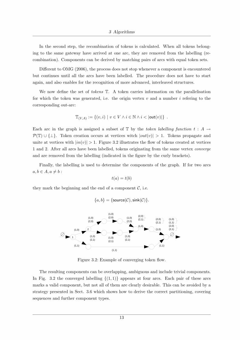
We now define the set of tokens T. A token carries information on the parallelisationfor which the token was generated, i.e. the origin vertex v and a number i refering to thecorresponding out-arc:

T(V,A) := {(v, i) | v ∈ V ∧ i ∈ N ∧ i < |out(v)|} .

Each arc in the graph is assigned a subset of T by the token labelling function t : A →P(T) ∪ {⊥}. Token creation occurs at vertices witch |out(v)| > 1. Tokens propagate andunite at vertices with |in(v)| > 1. Figure 3.2 illustrates the flow of tokens created at vertices1 and 2. After all arcs have been labelled, tokens originating from the same vertex convergeand are removed from the labelling (indicated in the figure by the curly brackets).

Finally, the labelling is used to determine the components of the graph. If for two arcsa, b ∈ A, a 6= b :

t(a) = t(b)

they mark the beginning and the end of a component C, i.e.

{a, b} = {source(C), sink(C)}.

1

2(1,0)

(1,1)

(1,1)

(1,1)

(1,0)(1,1)(2,0)(2,1)

(1,0)(2,0)

(1,0)(2,1)

(1,0)(2,0) (1,0)

(2,0)

(1,0)(2,1)

(1,0)(2,1)

(2,0)(2,1)

(1,0)

(2,0)(2,1)

(1,0)

Figure 3.2: Example of converging token flow.

The resulting components can be overlapping, ambiguous and include trivial components.In Fig. 3.2 the converged labelling {(1, 1)} appears at four arcs. Each pair of these arcsmarks a valid component, but not all of them are clearly desirable. This can be avoided by astrategy presented in Sect. 3.6 which shows how to derive the correct partitioning, coveringsequences and further component types.

13

3 Algorithms

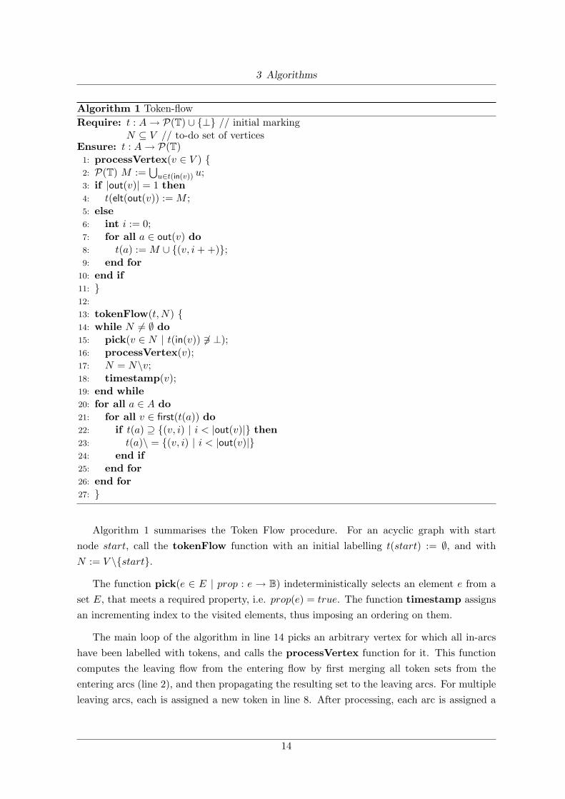
Algorithm 1 Token-flowRequire: t : A→ P(T) ∪ {⊥} // initial marking

N ⊆ V // to-do set of verticesEnsure: t : A→ P(T)

1: processVertex(v ∈ V ) {2: P(T) M :=

⋃u∈t(in(v)) u;

3: if |out(v)| = 1 then4: t(elt(out(v)) := M ;5: else6: int i := 0;7: for all a ∈ out(v) do8: t(a) := M ∪ {(v, i + +)};9: end for

10: end if11: }12:

13: tokenFlow(t, N) {14: while N 6= ∅ do15: pick(v ∈ N | t(in(v)) 63 ⊥);16: processVertex(v);17: N = N\v;18: timestamp(v);19: end while20: for all a ∈ A do21: for all v ∈ first(t(a)) do22: if t(a) ⊇ {(v, i) | i < |out(v)|} then23: t(a)\ = {(v, i) | i < |out(v)|}24: end if25: end for26: end for27: }

Algorithm 1 summarises the Token Flow procedure. For an acyclic graph with startnode start, call the tokenFlow function with an initial labelling t(start) := ∅, and withN := V \{start}.

The function pick(e ∈ E | prop : e → B) indeterministically selects an element e from aset E, that meets a required property, i.e. prop(e) = true. The function timestamp assignsan incrementing index to the visited elements, thus imposing an ordering on them.

The main loop of the algorithm in line 14 picks an arbitrary vertex for which all in-arcshave been labelled with tokens, and calls the processVertex function for it. This functioncomputes the leaving flow from the entering flow by first merging all token sets from theentering arcs (line 2), and then propagating the resulting set to the leaving arcs. For multipleleaving arcs, each is assigned a new token in line 8. After processing, each arc is assigned a

14

3 Algorithms

timestamp (line 18), which is later used to identify sequence-boundaries (see Sect. 3.6). Oncethe main loop in tokenFlow terminates, converged tokens are removed (line 22).

Our reference implementation (see Sect. 4) uses depth-first-search. Vertices and arcs arevisited once; thus the algorithm has a time-complexity in O(|V | + |A|). Using a hash map,identifying equally labelled arcs can be achieved in constant time.

3.3 Cycles Cause Deadlocks

Algorithm 1 only works for acyclic graphs. Vertex 1 in the cycle in Fig. 3.3 cannot beprocessed until the back-arc (4, 1) has been labelled; this however would require the flowleaving 1 be processed first, as it must pass along the vertices 2, 3 and 4. This results in adeadlock. All cycles have a back arc in the depth-first-search tree, pointing to a connectingvertex which cannot be processed because the required flow through the back-arc must passthrough the vertex itself; hence, the flow cannot proceed from there, causing a deadlock. Thefollowing chapter introduces a method to avoid this problem.

Figure 3.3: A deadlock at node 1.

3.4 Contracting Cycles

The following theorem provides an important insight into the meaning of cycles for the algo-rithm.

Theorem 3.4.1. Let c be a cycle, C = (VC , AC) a component. Then

source(C) ∈ arcs(c)⇔ sink(C) ∈ arcs(c) .

Proof. Let source(C) ∈ arcs(c) and assume sink(C) 6∈ arcs(c). For the path of the cycle withlength |c| = n define without loss of generality (c(n), (c(1)) = source(C). Thus the path startsat c(1) = to(source(C)). By induction over the path length of c, we show that ∀i : c(i) ∈ VC .For c(1) ∈ VC this is clearly true, as the source points to a vertex inside the component. Nowlet it be true for c(i). Applying Lemma 3.1.1 yields that c(i+1) ∈ VC , because (c(i), c(i+1)) 6=

15

3 Algorithms

sink(C), and the sink is the only arc that leaves the component. Then also c(n) ∈ VC . But(c(n), c(1)) = source(C) violates the definition of the source Ci), for (c(n), c(1)) ∈ AC . It isinside the component. This contradicts the assumption. The other implication follows inanalogy by the same argument in reverse direction: for the path along the cycle starting atthe sink, each predecessor must not be the source because of Lemma 3.1.1. Symmetrically,the same argument contradicts the definition of the sink Cii).

In other words, Theorem 3.4.1 states that source and sink of a component are never

positioned across the boundaries of any cycle. For example, in Fig. 3.4 (a) the boldarcs do not identify any component because only one belongs to a cycle the other does not.In (b) both arcs are in the same cycle and indicate a valid component. More restrictions forinter-cyclic components, as shown in (c), are discussed later.

No information on the location of components passes from the outside into any cycleinterior and vice versa. Tokens convey information on component boundaries. Thereforecycles can be isolated from the token flow without losing information.

(a) (b) (c)

Figure 3.4: Component boundaries do not cross cycle boundaries.

To achieve this, two requirements must be met: i) the flow around cycles (cycle exter-nal) and ii) the flow inside cycles (cycle internal) must lead to a correct identification ofcomponents.

The following sections introduce the necessary preparations to enable arbitrary cyclicgraphs to be processed by the token flow algorithm. In Sect. 3.4.1 we specify the externalflow, in Sect. 3.4.2 the behaviour of cycle internal flow, and in Sect. 3.4.3 we give a solutionto problems that arise when cycles are nested within others.

3.4.1 Cycle-External Flow.

Figure 3.5 shows two components C1 and C2 containing (simple) cycles. Each source and sinkpairs must carry the same token labelling: t(a2) != t(a1) = ∅ ∧ t(a4) != t(a3) = ∅.

To achieve this for C1, the tokens (v, 0) and (v, 1) flowing into the cycle must converge ata2. This could be achieved by tracking the tokens separately, as they would finally arrive ata2. For the flow inside the cycle is independent of the exterior , this is possible if all incoming

16

3 Algorithms

convergecreate

converge

C1 C2

a4

a3a1a2v

(v,0)

(v,1)

{ }

create

{ }

Figure 3.5: Cycle external flow.

flow merges by the cycle. In C2 the two branches flowing out of the cycle do not belong to thesame component and therefore must have a different token labelling. Clearly this cannot beachieved by tracking the tokens separately, for the arcs leaving the cycle in C2 would receivean equal labelling. In order to keep the branches separate the tokens must, again, be createdby the cycle itself.

Token creation and convergence are vertex properties. This gives rise to the idea of treatingcycles and vertices equally. For this purpose we introduce replacement vertices for cycles, andcall the process of embedding them into the graph contraction. Figure 3.6 illustrates theprocess: each arc ai is replaced by an arc a′i connecting with the replacement vertex.

a1

a2

a3

a4

a1' a

3'

a2'

a4'

Figure 3.6: A cycle is contracted to a replacement vertex.

To map a cycle c onto a vertex, we first determine its incoming and leaving flow. Formally,the connectivity of a cycle c to its environment is defined by the functions in and out in analogyto those of a vertex:

in(c) := {(u, v) ∈ A\arcs(c) | v ∈ vertices(c)},

out(c) := {(u, v) ∈ A\arcs(c) | u ∈ vertices(c)} .

To contract a cycle c, we need to set the references to the replacement vertex; for all enteringarcs a ∈ in(c), set to(a) := c and for all leaving arcs a ∈ out(c) set from(a) := c.

Note that unlike the vertices in BPDs, contracted cycles can have multiple in- and out-

17

3 Algorithms

flows. This is no limitation for the token-flow algorithm and does not effect model semantics.

Contraction is only a temporary process to determine the token labellings. Storing theoriginal references of the replaced arcs enables them to be restored after the algorithm hasfinished. Thus, the original input graph can be mapped to its corresponding components.

3.4.2 Cycle-Internal Flow.

After contraction, external flow does not arrive inside cycles. A means of boot-strappinginternal flow is required, similar to the ∅ labelling of the start arc. We define an initiallabelling at certain internal arcs for each cycle.

The places where to start naturally seem to be the vertices, that have a connection to theenvironment. We call internal vertices that are connected to a cycle c’s environment ports:

ports(c) := to(in(c)) ∪ from(out(c)) .

Ports of a cycle cannot be contained in internal components (see Fig. 3.4(c)): if a portwere included in a component then, because of its connection to the exterior, following fromLemma 3.1.1, some vertices of the environment would have to be included, too. Theorem3.4.1 states that this is not possible.

To ensure that ports are not identified as parts of components, each flow between twoports needs different token-ids. The token flow shall begin at the ports, so we set the initiallabelling at the out arcs of ports belonging to the cycle. Formally, they belong to the set

initflow(c) := out(ports(c)) ∩ arcs(c) .

Figure 3.7(a) depicts the ports and initflow arcs of a simple cycle. The initial tokens mustnot converge, as can be seen in Fig. 3.7(b): if the initial labellings t(a1) and t(a2) did convergeat vertex v, then t(a3) would be ∅ and thus a3 would falsely be identified with the in and out

arcs of the cycle.

v

{ } { }a1 a2

a3ports

initflow

(a) (b)

Figure 3.7: A cycle with its ports and initflow (a). Internal tokens do not converge (b).

Therefore, we expand the token set by a non-converging internal token type:

T(V,A) := {(v, i)| v ∈ V ∧ i ∈ N ∧ i < |out(v)|} ∪ {(int, i)| i ∈ N}

18

3 Algorithms

The initflow arcs must be labelled with different int- tokens. In Fig. 3.7(b) for instance,the labelling is t(a1) = {(int, 0)} and t(a2) = {(int, 1)}.

3.4.3 Substructure of Cycles.

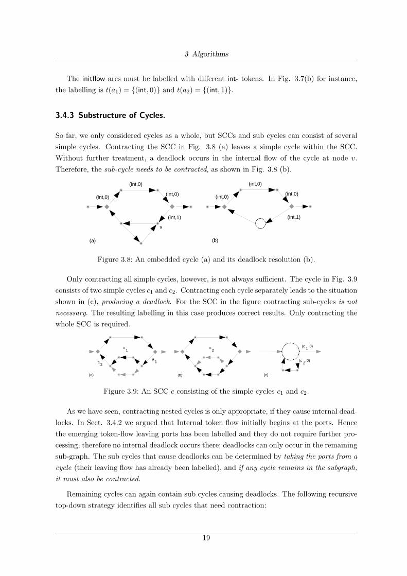
So far, we only considered cycles as a whole, but SCCs and sub cycles can consist of severalsimple cycles. Contracting the SCC in Fig. 3.8 (a) leaves a simple cycle within the SCC.Without further treatment, a deadlock occurs in the internal flow of the cycle at node v.Therefore, the sub-cycle needs to be contracted, as shown in Fig. 3.8 (b).

(int,1)

(int,0)

(int,0)

(int,0)

v

(int,1)

(int,0)

(int,0)

(int,0)

(a) (b)

Figure 3.8: An embedded cycle (a) and its deadlock resolution (b).

Only contracting all simple cycles, however, is not always sufficient. The cycle in Fig. 3.9consists of two simple cycles c1 and c2. Contracting each cycle separately leads to the situationshown in (c), producing a deadlock. For the SCC in the figure contracting sub-cycles is notnecessary. The resulting labelling in this case produces correct results. Only contracting thewhole SCC is required.

c1

c2

a1a

2

(c1, 0)

(c2, 0)

(a) (b) (c)

Figure 3.9: An SCC c consisting of the simple cycles c1 and c2.

As we have seen, contracting nested cycles is only appropriate, if they cause internal dead-locks. In Sect. 3.4.2 we argued that Internal token flow initially begins at the ports. Hencethe emerging token-flow leaving ports has been labelled and they do not require further pro-cessing, therefore no internal deadlock occurs there; deadlocks can only occur in the remainingsub-graph. The sub cycles that cause deadlocks can be determined by taking the ports from acycle (their leaving flow has already been labelled), and if any cycle remains in the subgraph,it must also be contracted.

Remaining cycles can again contain sub cycles causing deadlocks. The following recursivetop-down strategy identifies all sub cycles that need contraction:

19

3 Algorithms

1. Find all SCCs within the (sub-) graph.

2. Contract them.

3. Repeat step 1 on the subgraph of each found SCC without its ports.

Taking the ports from the cycle in Fig. 3.9 opens up both simple cycles c1 and c2; nosub-cycle is left, so only the top SCC is contracted. In Fig. 3.8(a) the sub-cycle does notcontain ports and thus is contracted. The remaining subgraphs are shown in Fig. 3.10.

(a) (b)

Figure 3.10: The SCCs without the ports.

Also note that taking the ports from a cycle leaves exactly those simple cycles intact, thatdo not contain any port vertices.

3.5 Preparations for the Token-flow Algorithm

Algorithm 2 makes the necessary preparations for the token flow algorithm on graphs con-taining cycles. The recursive function contractAll is initially called on the set containingall vertices of the graph. First all (non-trivial) SCCs are determined (line 21). Algorithmsfor detecting SCCs are broadly available, e.g. see Thomas H. Cormen (1994). Each SCC iscontracted (line 22) which returns the replacement vertex v. The contraction replaces the in

and out arcs incident on the cycle by new arcs incident on the new replacement vertex. Thenin line 23, the arcs are labelled for the initial flow by assigning each arc a unique token. Foreach SCC a recursive call (line 27) handles the sub-cycles, as described in Sect. 3.4.1.

3.6 Exploiting Results for Component Identification

From the arc labelling, components can be derived. Only some of them are useful, however.Components should be contained within a tree-like structure, meaning for two componentsthat either one is contained within the other (a child in the tree) or that they are disjoint (ondifferent branches). The only case where this might occur is within sequences. In Sect. 3.6.1their handling is described. Sect. 3.6.2 extends the token concept to enable the detection offurther structures.

20

3 Algorithms

3.6.1 Maximum Sequences.

If a token configuration exists only once, the arc is neither source nor sink. Two arcs withequally labelled token sets are source and the sink of a valid component. If the component istrivial, it only contains a single vertex and can be neglected. Non-trivial components are cycliccomponents if they contain any contracted vertices, otherwise they are acyclic components.

Whether an arc is a source or a sink is determined by its finishing timestamps of the tokenflow algorithm: the arc carrying the earlier timestamp is the source. This follows from theflow properties: in depth-first search, the source must be encountered before the sink arc.

More than two arcs with equal sets of tokens mean a sequence. Figure 3.11(a) depictsa simple chain with the labelling t(a1) = t(a2) = t(a3) = t(a4). Of all possible and validcomponents following from combinations of these tokens (e.g. source = a2, sink = a4), onlythe maximum sequence is of interest; it contains all subsequences. The maximum sequencecomponent C1 can be identified by the finishing timestamps: its source carries the earliest andthe sink the latest timestamp.In the example: source(C1) = a1, sink(C1) = a4.

a1

a2

a3 a

4a

5

C1

C2

C3

C4

a1

a2

a3

a4

C1

(a) (b)

Figure 3.11: Sequence Components.

Sequences can also contain sub-components, like C4 containing C1, C2, C3 in Fig. 3.11(b).Each subcomponent is located between a pair ai, ai+1. The pair (a1, a2) belongs to a cyclecomponent, whereas the pairs (a2, a3) and (a4, a5) belong to acyclic components, and (a3, a4)is trivial. Eventually, component C4 maps to a sequence including three components and onesingle vertex.

To summarise the component identification for arcs with equal labellings:

• For exactly two equally labelled arcs, add a component (if non-trivial).

• For more, add a sequence for the earliest and latest labelled arc.

• For each pair of arcs with succeeding timestamps, add a component (if non-trivial).

Token analysis yields a classification of components into three categories, which can beused to associate the derived components with concrete BPEL elements:

• Cyclic components containing contracted vertices either translate to <while> or <repeat>activities or can be translated using event handlers, as in Ouyang, Dumas, ter Hofstede& van der Aalst (2006a).

21

3 Algorithms

• acyclic components translate to <switch>, <pick> and <flow> activities (flow pattern-based translation in Ouyang et al. (2007) can be used here), and

• sequence components.

3.6.2 Partial Convergence.

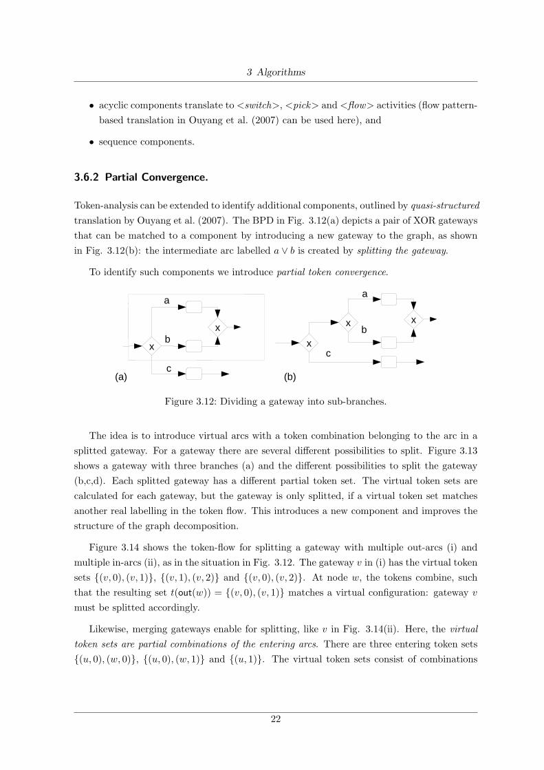
Token-analysis can be extended to identify additional components, outlined by quasi-structuredtranslation by Ouyang et al. (2007). The BPD in Fig. 3.12(a) depicts a pair of XOR gatewaysthat can be matched to a component by introducing a new gateway to the graph, as shownin Fig. 3.12(b): the intermediate arc labelled a ∨ b is created by splitting the gateway.

To identify such components we introduce partial token convergence.

bx

a

x

c(a)

bx

a

x

xc

(b)

Figure 3.12: Dividing a gateway into sub-branches.

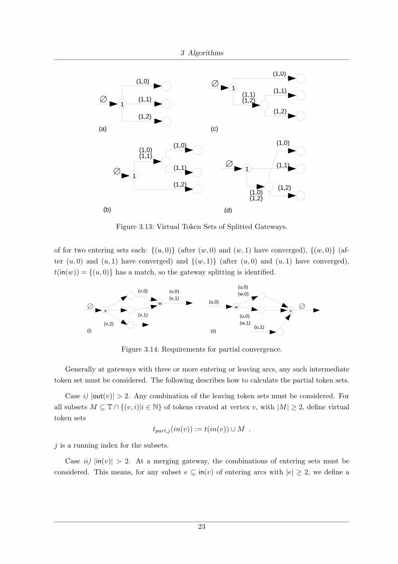
The idea is to introduce virtual arcs with a token combination belonging to the arc in asplitted gateway. For a gateway there are several different possibilities to split. Figure 3.13shows a gateway with three branches (a) and the different possibilities to split the gateway(b,c,d). Each splitted gateway has a different partial token set. The virtual token sets arecalculated for each gateway, but the gateway is only splitted, if a virtual token set matchesanother real labelling in the token flow. This introduces a new component and improves thestructure of the graph decomposition.

Figure 3.14 shows the token-flow for splitting a gateway with multiple out-arcs (i) andmultiple in-arcs (ii), as in the situation in Fig. 3.12. The gateway v in (i) has the virtual tokensets {(v, 0), (v, 1)}, {(v, 1), (v, 2)} and {(v, 0), (v, 2)}. At node w, the tokens combine, suchthat the resulting set t(out(w)) = {(v, 0), (v, 1)} matches a virtual configuration: gateway v

must be splitted accordingly.

Likewise, merging gateways enable for splitting, like v in Fig. 3.14(ii). Here, the virtualtoken sets are partial combinations of the entering arcs. There are three entering token sets{(u, 0), (w, 0)}, {(u, 0), (w, 1)} and {(u, 1)}. The virtual token sets consist of combinations

22

3 Algorithms

1

(1,0)

(1,1)

(1,2)

1

(1,0)(1,1)

(1,1)

(1,2)

(1,0)

1(1,1)(1,2)

(1,2)

(1,0)

(1,1)

1

(1,2)

(1,0)

(1,1)

(1,0)(1,2)

(a)

(b)

(c)

(d)

Figure 3.13: Virtual Token Sets of Splitted Gateways.

of for two entering sets each: {(u, 0)} (after (w, 0) and (w, 1) have converged), {(w, 0)} (af-ter (u, 0) and (u, 1) have converged) and {(w, 1)} (after (u, 0) and (u, 1) have converged).t(in(w)) = {(u, 0)} has a match, so the gateway splitting is identified.

vw

(v,0)(v,1)

(i)

wv

(u,0)

(ii)

(u,0)(w,0)

(u,0)(w,1)

(u,1)

(v,0)

(v,1)

(v,2)

Figure 3.14: Requirements for partial convergence.

Generally at gateways with three or more entering or leaving arcs, any such intermediatetoken set must be considered. The following describes how to calculate the partial token sets.

Case i) |out(v)| > 2. Any combination of the leaving token sets must be considered. Forall subsets M ⊆ T ∩ {(v, i)|i ∈ N} of tokens created at vertex v, with |M | ≥ 2, define virtualtoken sets

tpart,j(in(v)) := t(in(v)) ∪M .

j is a running index for the subsets.

Case ii) |in(v)| > 2. At a merging gateway, the combinations of entering sets must beconsidered. This means, for any subset e ⊆ in(v) of entering arcs with |e| ≥ 2, we define a

23

3 Algorithms

virtual token set tpart of the tokens:

tpart,j(out(v)) :=⋃

u∈t(e)

u .

There are 2|out(v)|− |out(v)| − 2 partial combinations for case i) and 2|in(v)|− |in(v)| − 2 forcase ii). Token analysis must consider partial tokens for AND and XOR gateways. Tokensin tpart converge in the usual way. If tokens match with partial arcs, they are generated bysplitting gateways (as shown in Fig. 3.12). For instance, if t(a) = tpart(b) then the gatewaynode b is divided, generating a new valid component. If the gateway type is XOR, guardconditions need to be handled. The guard-condition of the intermediate arc is the disjunctionof the guards of the corresponding splitted branches.

24

3 Algorithms

Algorithm 2 Mark initial flow and contract SCCs.Require: (V,A) directed graphEnsure: t : A→ P(T) ∪ {⊥} // initial marking

N ⊆ V // to-do set of vertices1: Init: N := V \{start};2: t(start) := ∅;3: int i := 0; // counter for int tokens4: contractAll(V );5:

6: contract(c ∈ V ∗){7: V v; //new replacement vertex8: V ∪ = {v};9: for all a ∈ in(c) do

10: A ∪ = (from(a), v);11: A \ = a;12: end for13: for all a ∈ out(c) do14: A ∪ = (v, to(a));15: A \ = a;16: end for17: return v;18: }19:

20: contractAll(V ′ ⊆ V ){21: for all s ∈ SCCs(V ′) do22: V v := contract(s);23: for all a ∈ initflow(s) do24: t(a) := {(int, i + +)};25: end for26: N \ = ports(s);27: contractAll(vertices(s)\ports(s));28: end for29: }

25

4 Use Case

We now demonstrate Token Analysis and our proof-of-concept implementation. It can bedownloaded from http://sourceforge.net/projects/tokenanalysis/. The following presentsin detail all the different mapping steps from the BPD input model to the final BPEL code.We use a realistic example to give an overview of how techniques described in Sect. 3 worktogether.

We show the single steps of the transformation with a sample process graph for qualitycontrol in Fig. 4.1 (the graph is used for demonstration only. A real process graph would bemuch more complex).

AnalysePerformance+

x

CalculateFailure

Frequency

+ UpdateStatistics

Derivepossible

Improvements

ProduceItem

QualityCheck x

RepairDemage

fail

EvaluateResultx

Rate Item'Class B'

Prepare Itemfor Shippingx

+

pass

pass

fail

Figure 4.1: A BPD for Quality Control of Production.

The first step in analysis is, according to Sect. 3.4 the identification of the SCCs that needto be contracted. The graph contains one SCC (2, 3, 4, 5, 6, 7, 8) with ports 2, 5, and 8.(Fig.4.2).

Taking the ports from the only SCC in Fig. 4.2 leaves no internal SCCs, as shown in Fig.4.3. Thus, only one SCC needs to be contracted to the replacement vertex SCC 0. Next,the initflow arcs of the cycle, (2, 3), (5, 6), and (8, 2), are given internal token labels along theinit-flow arcs for boot-strapping. The result is shown in Fig. 4.4.

The token flow algorithm is launched for the initial labelling of the SCC and an ∅ labelat (S, 1). First consider cycle external flow. Figure 4.5 shows the flow around the contractedvertex SCC 0 and the token configurations for the arcs, after token convergence.

26

4 Use Case

S 121

2

13

14 15 16

3 4 5

678

9

1110

17 E

SCC 0

Figure 4.2: One SCC in the Quality Control Graph.

3 4

67

SCC 0

Figure 4.3: The SCC without its Ports.

There are 3 tokens created at vertex 1. Therefore, additional partial token configurationsare created; they are {(1, 0), (1, 1)}, {(1, 1), (1, 2)} and {(1, 0), (1, 2)}.The first token (1, 0)enters the cycle replacement vertex. SCC 0 has two leaving arcs (8, 9), (5, 10). Here thereplacement vertex creates 2 new tokens (SCC 0, 0) and (SCC 0, 1). The tokens propagatealong the flow and at vertex 10, the ones belonging to SCC 0 converge. At an intermediatearc of vertex 1 there is a partial match with the arc (14, 15) carrying the tokens {(1, 1), (1, 2)}.Thus the gateway is splitted; the result of the splitting is depicted in Fig. 4.6, together withthe remaining internal flow. Finally, all branches merge back at 17.

In the cycle internal flow no branching takes place. Therefore the tokens simply propagateup to the next ports.

2 3 4 5

678

SCC 0

(int,1)

(int,0)

(int,2)

Figure 4.4: The init Flow for the SCC.

27

4 Use Case

S 121

13

14 15 16

9

1110

17 E

SCC 0(1,0)

(1,0)

(1,0)(SCC 0, 1)

(1,0)(SCC 0, 1)

(1,0)(SCC 0, 0)(1,0)

(1,1)

(1,2)

(1,1)(1,2)

(1,1)(1,2)

(1,1)(1,2)

(1,1)(1,2)

(1,0)(1,2)

(1,0)(1,1)

partial arcs

Figure 4.5: Cycle External Flow in the Control Graph.

S12

1

2

13

14 15 16

3 4 5

678

9

1110

17 E1part

(1,0)(SCC 0, 1)

(1,0)

(1,1)(1,2)

(1,2)

(1,1)

(1,2)

(1,1)

(int,1) (int,1) (int,1)

(int,0)

(int,0)(int,0)

(1,0)(SCC 0, 1)

(int,2)

(1,1)(1,2)

(1,1)(1,2)

(1,1)(1,2)

(1,0)(SCC 0, 0) (1,0)

(1,0)

Figure 4.6: Token Flow in the Control Graph.

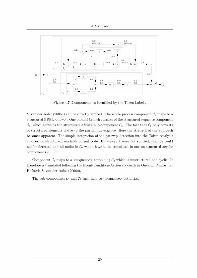
Figure 4.7 shows the resulting process graph with the final token sets.

In the next step, components are identified by arcs with equal token sets. The pair(S, 1) → (17, E) marks the super component C7 representing the entire scope. The arcs(1, 2), (10, 11), (11, 17) have the same labelling. According to the rules in Sect. 3.6.1, theymust form a sequence, therefore the outer pair of arcs (1, 2)→ (11, 17) belongs to the sequencecomponent C4. Inside there is one non-trivial sub-component (1, 2) → (10, 11) that includesthe SCC (cyclic component C3) and one trivial component, which is omitted. Inside the cycleexist two further sequences C1 : (5, 6) → (7, 8) and C2 : (2, 3) → (4, 5) with only trivial sub-sequences. The partial arc (1, 1part) matches the arcs flowing out from 14 and therefore thepartial component C5 is created. The subsequence 15 to 17 contains only trivial components.The whole identified sequence C6 is (1, 1part)→ (16, 17).

The final step is the model translation to BPEL. As the correspondence of graph elementsto BPEL blocks has now been established, the techniques from Ouyang, Dumas, ter Hofstede

28

4 Use Case

S12

1

2

13

14 15 16

3 4 5

678

9

1110

17 E1

part

(1,0)(SCC 0, 1)

(1,0)

(1,1)(1,2)

(1,2)

(1,1)

(1,2)

(1,1)

(int,1) (int,1) (int,1)

(int,0)

(int,0)(int,0)

(1,0)(SCC 0, 1)

(int,2)

(1,1)(1,2)

(1,1)(1,2)

(1,1)(1,2)

(1,0)(SCC 0, 0) (1,0)

(1,0)

C5

C1

C2

C6

C3C

4

C7

Figure 4.7: Components as Identified by the Token Labels.

& van der Aalst (2006a) can be directly applied. The whole process component C7 maps to astructured BPEL <flow>. One parallel branch consists of the structured sequence componentC6, which contains the structured <flow> sub-component C5. The fact that C6 only consistsof structured elements is due to the partial convergence. Here the strength of the approachbecomes apparent. The simple integration of the gateway detection into the Token Analysisenables for structured, readable output code. If gateway 1 were not splitted, then C6 couldnot be detected and all nodes in C6 would have to be translated in one unstructured acycliccomponent C7.

Component C4 maps to a <sequence> containing C3 which is unstructured and cyclic. Ittherefore is translated following the Event-Condition-Action approach in Ouyang, Dumas, terHofstede & van der Aalst (2006a).

The sub-components C1 and C2 each map to <sequence> activities.

29

5 Conclusion

We have demonstrated how Token-Flow can be used to identify the components of a processgraph. The identification works for cyclic graphs, too. Describing the necessary steps, wegathered theory results for cycles, that yield a cycle internal and external view of the flow. Theapproach also provides a classification of the components (sequence, cyclic, flow) allowing tospeed up further translation steps; the actual mapping to code can be achieved with methodsdescribed in Ouyang, Dumas, ter Hofstede & van der Aalst (2006a), Ouyang et al. (2007).Also, the described approach enables for detection of partial components, that cannot beidentified by simply checking the definition of components. Our implementation has alreadybeen successfully employed in the workflow code generation framework (Roser et al (2007))which is e.g. used in AgilPro (www.agilpro.eu). The workflow code generation frameworkprovides adapters in order to connect it to different modeling tools, transforms the graph asdescribed above and generates code according to predefined code-templates.

We also see high potential that our work can contribute to improve the bridge betweenprocess modelling and workflow execution in practice. Process modelling approaches and toolswill benefit, since restrictions on the process models towards execution with BPEL workflowengines can be reduced. The extended component identification also provides a basis todisplay changes in the workflow code in the process model more easily. This kind of reverseengineering will be a topic of future research. Also, a formal analysis and proof of correctnessis left as future work.

30

Bibliography

Ammarguellat, Z. (1992), ‘A control-flow normalization algorithm and its complexity’, Softw.Engin. 13, 237–251.

BOC (2007), ‘Prozessorientierte Anwendungsentwicklung mit ADONIS : Konzepte, Servicesund Beratungsleistungen der BOC’, Whitepaper.

Gupta, R. & Soffa, M. L. (1978), ‘Region scheduling’, 2nd Int. Conf. on Supercomp. pp. 141–148.

Havlak, P. (1997), ‘Nesting of reducible and irreducible loops’, ACM Trans. Program. Lang.Syst. 19(4), 557–567.

IBM (2006), ‘Best practices for using websphere business modeler and monitor’, Redpaper.http://www.redbooks.ibm.com/redpapers/pdfs/redp4159.pdf.

Jablonski, S. & Bussler, C. (1996), Workflow Management - Modeling Concepts, Architectureand Implementation, Thomson Computer Press.

Johnson, R., Pearson, D. & Pingali, K. (1994), The program structure tree: computing controlregions in linear time, in ‘PLDI ’94: Proceedings of the ACM SIGPLAN 1994 conferenceon Programming language design and implementation’, ACM Press, New York, NY, USA,pp. 171–185.

Koehler, J. & Hauser, R. (2004), Untangling Unstructured Cyclic Flows - A Solution Basedon Continuations, in ‘In Proceedings of the OTM Confederated International Conferences’,Vol. 3290 of LNCS, Springer, pp. 121–138.

Mendling, J., Lassen, K. & Zdun, U. (2006), ‘Transformation Strategies between Block-Oriented and Graph-Oriented Process Modelling Languages’, MKWI 2, 297–312.

Nagy, R. (n.d.), ‘MDD trifft SOA’, Whitepaper. http://www.microtool.de/mt/pdf/

objectif/49/mdd_soa.pdf.

OASIS (2003), Business Process Execution Language for Web Services (WS-BPEL) Version1.1.

Oliver Pera, M. (2007), ‘Innovator 2007: Von geschaftsprozessen zu web services odervon business zu bpel’, Whitepaper. http://www.mid.de/fileadmin/documents/pdf/

WhitePapers/Innovator_2007_WhitePaper_B2BPEL_070205.pdf.

i

Bibliography

OMG (2006), Business Process Modeling Notation (BPMN) Version 1.0. http://www.bpmn.org/Documents/OMG%20Final%20Adopted%20BPMN%201-0%20Spec%2006-02-01.pdf.

Oracle (n.d.), ‘Oracle SOA Suite - Oracle BPEL Process Manager’.

Ouyang, C., Dumas, M., Breutel, S. & ter Hofstede, A. H. (2006), Translating StandardProcess Models to BPEL, in ‘Proceedings of CAiSE 2006’, Vol. 4001 of LNCS, Springer,pp. 417–432.

Ouyang, C., Dumas, M., ter Hofstede, A. H. & van der Aalst, W. M. (2006a), ‘From BPMNProcess Models to BPEL Web Services’, IEEE ICWS pp. 285–292.

Ouyang, C., Dumas, M., ter Hofstede, A. H. & van der Aalst, W. M. (2006b), ‘From BusinessProcess Models to Process-oriented Sofware Systems: The BPMN to BPEL Way’, BPMCenter Report BPM-06-27.

Ouyang, C., Dumas, M., ter Hofstede, A. H. & van der Aalst, W. M. (2007), ‘Pattern-basedtranslation of bpmn process models to bpel web services’, Internat. Journal of Web ServicesResearch JSWR .

Ramalingam, G. (2000), On loops, dominators, and dominance frontier, in ‘PLDI ’00: Pro-ceedings of the ACM SIGPLAN 2000 conference on Programming language design andimplementation’, ACM Press, New York, NY, USA, pp. 233–241.

Recker, J. & Mendling, J. (2006), ‘On the Translation between BPMN and BPEL: Concep-tual Mismatch between Process Modeling Languages’, CAiSE 2006 Workshop Proceedingspp. 521–532.

Roser et al, S. (2007), Generation of Workflow Code from DSMs, in ‘Proceedings of the 7thOOPSLA Workshop on Domain-Specific Modeling’, Montreal, Canada.

Tarjan, R. E. (1974), ‘Testing flow graph reducibility’, J. Comput. Syst. Sci. 9, 355–365.

Thomas H. Cormen, Charles E. Leiserson, R. L. R. (1994), Introduction to Algorithms, TheMIT electrical engineering and comp. sci. series, MIT Press, Cambridge.

van der Aalst, W. M. & Lassen, K. B. (2007), ‘Translating Unstructured Workflow Processesto Readable BPEL: Theory and Implementation’, Inf. and Softw. Techn. .

Wahli, U. et al. (2006), Business Process Management: Modeling through Monitoring UsingWebSphere V6 Products. IBM Redbook.

White, S. (2005), Mapping BPMN to BPEL example, Technical report, IBM. http://www.

bpmn.org/Documents/Mapping%20BPMN%20to%20BPEL%20Example.pdf.

Zhang, F. & D’Hollander, E. H. (2004), ‘Using hammock graphs to structure programs’, IEEETrans. Softw. Eng. 30(4), 231–245.

ii

List of Figures

3.1 Components do not contain start events. . . . . . . . . . . . . . . . . . . . . . . 123.2 Example of converging token flow. . . . . . . . . . . . . . . . . . . . . . . . . . 133.3 A deadlock at node 1. . . . . . . . . . . . . . . . . . . . . . . . . . . . . . . . . 153.4 Component boundaries do not cross cycle boundaries. . . . . . . . . . . . . . . 163.5 Cycle external flow. . . . . . . . . . . . . . . . . . . . . . . . . . . . . . . . . . 173.6 A cycle is contracted to a replacement vertex. . . . . . . . . . . . . . . . . . . . 173.7 A cycle with its ports and initflow (a). Internal tokens do not converge (b). . . 183.8 An embedded cycle (a) and its deadlock resolution (b). . . . . . . . . . . . . . . 193.9 An SCC c consisting of the simple cycles c1 and c2. . . . . . . . . . . . . . . . . 193.10 The SCCs without the ports. . . . . . . . . . . . . . . . . . . . . . . . . . . . . 203.11 Sequence Components. . . . . . . . . . . . . . . . . . . . . . . . . . . . . . . . . 213.12 Dividing a gateway into sub-branches. . . . . . . . . . . . . . . . . . . . . . . . 223.13 Virtual Token Sets of Splitted Gateways. . . . . . . . . . . . . . . . . . . . . . . 233.14 Requirements for partial convergence. . . . . . . . . . . . . . . . . . . . . . . . 23

4.1 A BPD for Quality Control of Production. . . . . . . . . . . . . . . . . . . . . . 264.2 One SCC in the Quality Control Graph. . . . . . . . . . . . . . . . . . . . . . . 274.3 The SCC without its Ports. . . . . . . . . . . . . . . . . . . . . . . . . . . . . . 274.4 The init Flow for the SCC. . . . . . . . . . . . . . . . . . . . . . . . . . . . . . 274.5 Cycle External Flow in the Control Graph. . . . . . . . . . . . . . . . . . . . . 284.6 Token Flow in the Control Graph. . . . . . . . . . . . . . . . . . . . . . . . . . 284.7 Components as Identified by the Token Labels. . . . . . . . . . . . . . . . . . . 29

iii