univariate and multivariate statistical distributions · pdf filebivariate statistics ......

Univariate and Multivariate Statistical Distributions

Multivariate Methods in EducationERSH 8350

Lecture #3 – August 31, 2011

ERSH 8350: Lecture 3

Today’s Lecture

• Univariate and multivariate statistics

• The univariate normal distribution

• The multivariate normal distribution

• How to inspect whether data are normally distributed

ERSH 8350: Lecture 3 2

Motivation for Today’s Lecture

• The univariate and multivariate normal distributions serve as the backbone of the most frequently used statistical procedures They are very robust and very useful

• Understanding their form and function will help you learn about a whole host of statistical routines immediately This course is essentially a course based in normal distributions


Today’s Example

• For today, we will use hypothetical data on the heights and weights of 50 students picked at random from the University of Georgia

• You can follow along in SAS using the example syntax and the data file “heightweight.csv”

0

50

100

150

200

250

300

50 55 60 65 70 75 80

Wei

ght (

in p

ound

s)

Height (in inches)


Random VariablesA random variable is a variable whose outcome depends on the result of chance

• Can be continuous or discrete Example of continuous: represents the height of a person, drawn at

random Example of discrete: represents the gender of a person, drawn at

random• Had a density function that indicates relative frequency

of occurrence A density function is a mathematical function that gives a rough

picture of the distribution from which a random variable is drawn

We will discuss the ways that are used to summarize a random variable


UNIVARIATE STATISTICS


Mean

The mean is a measure of central tendency• For a single variable, (put into a column vector):

( is a column vector with elements all 1 – size N x 1)

• The sampling distribution of Converges to normal as N increases (central limit theorem)

• In our data: mean height: ̅ 67.28 (in inches)


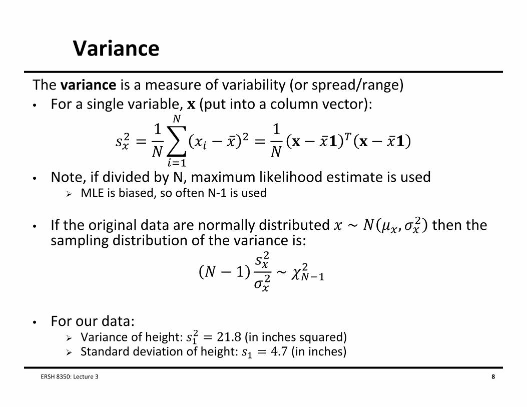
VarianceThe variance is a measure of variability (or spread/range)• For a single variable, (put into a column vector):

1̅

1̅ ̅

• Note, if divided by N, maximum likelihood estimate is used MLE is biased, so often N‐1 is used

• If the original data are normally distributed ∼ , then the sampling distribution of the variance is:

1 ∼

• For our data: Variance of height: 21.8 (in inches squared) Standard deviation of height: 4.7 (in inches)


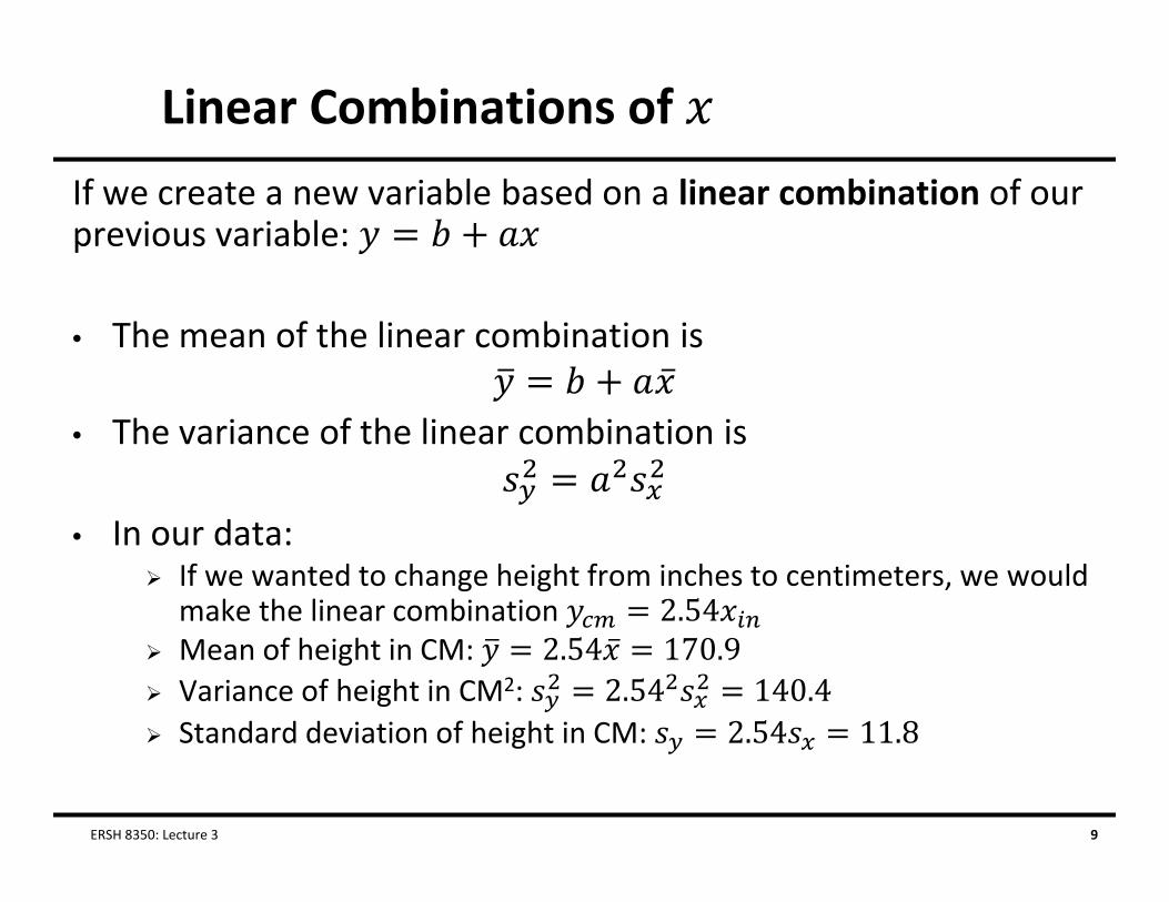
Linear Combinations of If we create a new variable based on a linear combination of our previous variable:

• The mean of the linear combination is

• The variance of the linear combination is

• In our data: If we wanted to change height from inches to centimeters, we would

make the linear combination 2.54 Mean of height in CM: 2.54 ̅ 170.9 Variance of height in CM2: 2.54 140.4 Standard deviation of height in CM: 2.54 11.8


UNIVARIATE STATISTICAL DISTRIBUTIONS


Univariate Normal Distribution

• For a continuous random variable (ranging from to ) the univariate normal distribution function is:

• The shape of the distribution is governed by two parameter: The mean The variance

• The skewness (lean) and kurtosis (peakedness) are fixed

• Standard notation for normal distributions is ERSH 8350: Lecture 3 11

Univariate Normal Distribution

For any value of , gives the height of the curve (relative frequency)


Chi‐Square Distribution• Another frequently used univariate distribution is the Chi‐

Square distribution Previously we mentioned the sampling distribution of the variance

followed a Chi‐Square distribution

• For a continuous (i.e., quantitative) random variable (ranging from to ), the chi‐square distribution is given by:

• is called the gamma function• The chi‐square distribution is governed by one parameter:

(the degrees of freedom) The mean is equal to ; the variance is equal to 2


(Univariate) Chi‐Square Distribution


Uses of Distributions• Statistical models make distributional assumptions on various

parameters and/or parts of data

• These assumptions govern: How models are estimated How inferences are made How missing data may be imputed

• If data do not follow an assumed distribution, inferences may be inaccurate Sometimes a problem, other times not so much

• Therefore, it can be helpful to check distributional assumptions prior to (or while) running statistical analyses


Assessing Distributional Assumptions Graphically

• A useful tool to evaluate the plausibility of a distributional assumption is that of the Quantile versus Quantile Plot (Q‐Q plot)

• A Q‐Q plot is formed by comparing the observed quantiles of a variable with that of a known statistical distribution A quantiles is the particular ordering of a given observation In our data, a person with a height of 71 is the 39th tallest person (out of 50)

This would correspond to the person being at the . .77 or .77 quantile of the distribution Taller than 77% of the distribution, or at the 77th percentile


Q‐Q Plot

• A Q‐Q Plot is built by:1. Ordering the data from smallest to largest2. Calculating the quantiles of each data point3. Looking up the quantiles of each data point using a known

statistical distribution4. Plotting the data against the value predicted by the

theoretical statistical distribution

• If the data deviate from a straight line, the data are not likely to follow from that theoretical distribution


Q‐Q Plot Example

• Using the example Excel spreadsheet, Q‐Q plots of our height data were built, comparing the data with a normal distribution (left) and a chi‐square distribution (right) The line is where the data “should” be if they followed that distribution

50

55

60

65

70

75

80

50 55 60 65 70 75 80

Normal Distribution

40

50

60

70

80

90

100

40 50 60 70 80 90 100

Chi-Square Distribution


BIVARIATE STATISTICS AND DISTRIBUTIONS


Bivariate Statistics

• Up to this point, we have focused on only one of our variables: height Looked at its marginal distribution (the distribution of it independent of that of weight)

Could have looked at weight, marginally

• Multivariate statistics is about exploring joint distributions How variables relate to each other

• As such, we will now look at the joint distributions of two variables or in matrix form: (size N x 2) Beginning with two, then moving to anything more than two


Multiple Means: The Mean Vector

• We can use a vector to describe the set of means for our data

Here is a N x 1 vector of 1s The resulting mean vector is a p x 1 vector of means

• For our data:


Mean Vector: Graphically

• The mean vector is the center of the distribution of both variables

0

50

100

150

200

250

300

50 55 60 65 70 75 80

Wei

ght (

in p

ound

s)

Height (in inches)


Covariance of a Pair of Variables

• The covariance is a measure of the relatedness Expressed in the product of the units of the two

The covariance between height and weight was 155.4 (in inch‐pounds)

The denominator N is the ML version – unbiased is N‐1

• Because the units of the covariance are difficult to understand, we more commonly describe association (correlation) between two variables with correlation Covariance divided by the product of each variable’s standard deviation


Correlation of a Pair of Varibles

• Correlation is covariance divided by the product of the standard deviation of each variable:

The correlation between height and weight was 0.72

• Correlation is unitless – it only ranges between ‐1 and 1 If and had variances of 1, the covariance between them would be a correlation Covariance of standardized variables = correlation


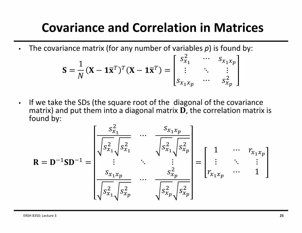
Covariance and Correlation in Matrices• The covariance matrix (for any number of variables p) is found by:

1 ⋯⋮ ⋱ ⋮

⋯

• If we take the SDs (the square root of the diagonal of the covariance matrix) and put them into a diagonal matrix , the correlation matrix is found by:

⋯

⋮ ⋱ ⋮

⋯

1 ⋯⋮ ⋱ ⋮

⋯ 1


Example Covariance Matrix• For our data, the covariance matrix was:

21.8 158.6158.6 2,260.2

• The diagonal matrix was:21.8 00 2,260.2

• The correlation matrix was:121.8

0

01

2,260.2

21.8 158.6158.6 2,260.2

121.8

0

01

2,260.2 1.00 0.72

0.72 1.00


Generalized Variance• The determinant of the sample covariance matrix is called the

generalized variance

• It is a measure of spread across all variables Reflecting how much overlap (covariance) in variables occurs in the

sample Amount of overlap reduces the generalized sample variance

• The generalized sample variance is: Largest when variables are uncorrelated Zero when variables form a linear dependency

• In data: The generalized variance is seldom used descriptively, but shows up

more frequently in maximum likelihood functions


Total Sample Variance• The total sample variance is the sum of the variances of each

variable in the sample The sum of the diagonal elements of the sample covariance matrix The trace of the sample covariance matrix

tr

• The total sample variance does not take into consideration the covariances among the variables Will not equal zero if linearly dependency exists

• In data: The total sample variance is commonly used as the denominator

(target) when calculating variance accounted for measuresERSH 8350: Lecture 3 28

BIVARIATE NORMAL DISTRIBUTION


Bivariate Normal Distribution

• The bivariate normal distribution is a statistical distribution for two variables Both variable is normally distributed marginally (by itself) Together, they form a bivariate normal distribution

• The bivariate normal density provides the relatively frequency of observing any pair of observations,

Where


Bivariate Normal Plot #1

Density Surface (3D) Density Surface (2D): Contour Plot


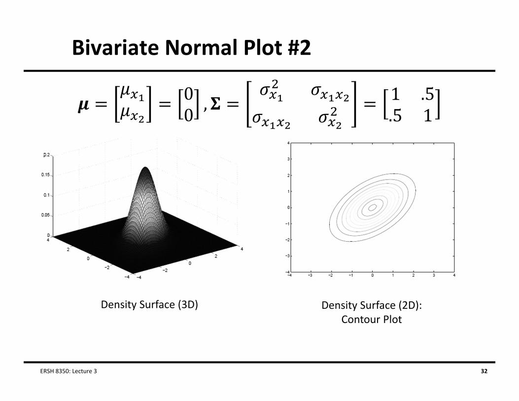
Bivariate Normal Plot #2



MULTIVARIATE DISTRIBUTIONS (VARIABLES ≥ 2)


Multivariate Normal Distribution

• The multivariate normal distribution is the generalization of the univariate normal distribution to multiple variables The bivariate normal distribution just shown is part of the MVN

• The MVN provides the relative likelihood of observing all p variables for a subject i simultaneously:

• The multivariate normal density function is:


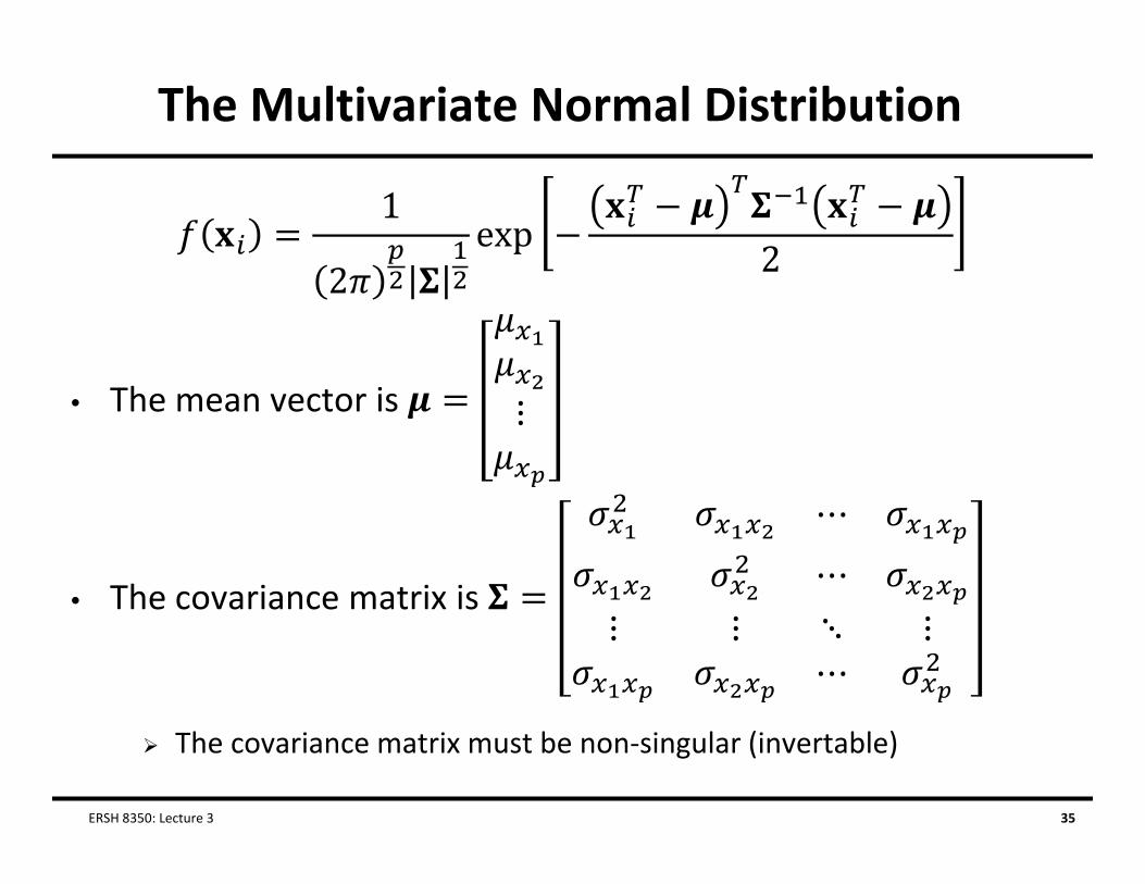
The Multivariate Normal Distribution

• The mean vector is

• The covariance matrix is

The covariance matrix must be non‐singular (invertable)


Multivariate Normal Notation

• Standard notation for the multivariate normal distribution of p variables is Our bivariate normal would have been ,

• In data: The multivariate normal distribution serves as the basis for most every statistical technique commonly used in the social and educational sciences General linear models (ANOVA, regression, MANOVA) General linear mixed models (HLM/multilevel models) Factor and structural equation models (EFA, CFA, SEM, path models) Multiple imputation for missing data

Simply put, the world of commonly used statistics revolves around the multivariate normal distribution Understanding it is the key to understanding many statistical methods


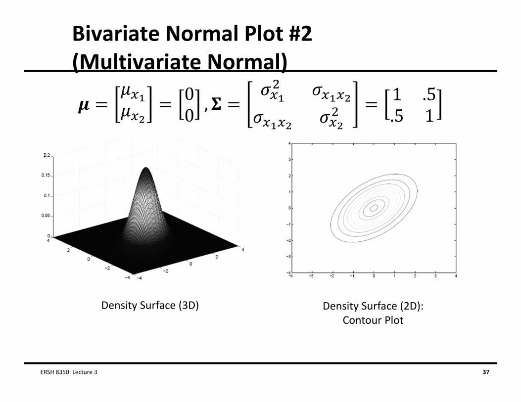
Bivariate Normal Plot #2 (Multivariate Normal)



Multivariate Normal Properties

• The multivariate normal distribution has some useful properties that show up in statistical methods

• If is distributed multivariate normally:1. Linear combinations of are normally distributed2. All subsets of are multivariate normally distributed3. A zero covariance between a pair of variables of

implies that the variables are independent4. Conditional distributions of are multivariate normal


Property #1: Linear Combinations• If then any set of linear combinations of

variables are also normally distributed as:

• If we had three variables and we wanted to create a new variable that was the difference between

and then:

For :

For :


More one Linear Combinations

• The linear combinations property is useful in several areas of statistics: Principal components (can determine mean and variance of each component)

Regression/ANOVA (can determine error of prediction for Y)

• We will see this property later in the course


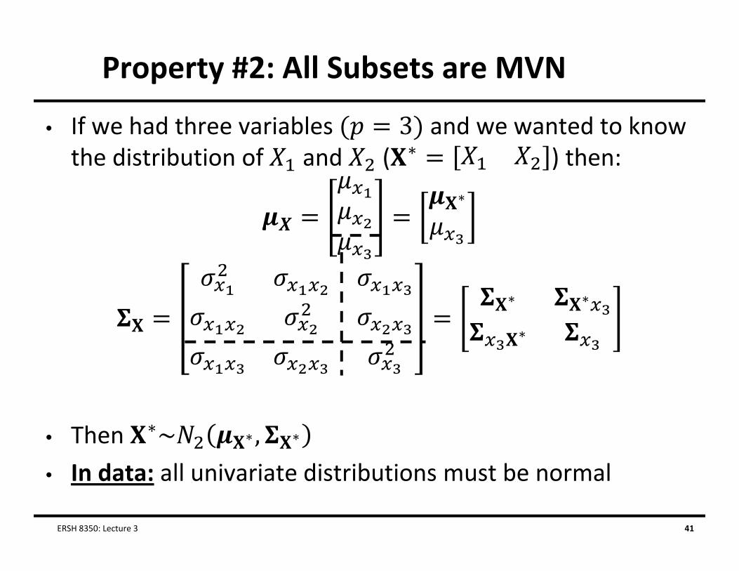
Property #2: All Subsets are MVN

• If we had three variables and we wanted to know the distribution of and ( ∗ ) then:

∗

∗ ∗

∗

• Then ∗ ∗ ∗

• In data: all univariate distributions must be normal


Property #3: Zero Covariance = Independence

• As we will see shortly, all of the information about the multivariate normal distribution is contained within the mean vector and the covariance matrix No other statistics are needed if you have these

• Therefore, if a pair of variables has a zero covariance (meaning zero correlation), then they are independent No other way dependency can happen (no higher moments that are variables)

• Important: this property is not true of all distributions Especially distributions for categorical data


Property #4: Conditional Distributions of Variables are Multivariate Normal

• The conditional distribution of sets of variables from a MVN is also MVN This is how missing data get imputed

• If we were interested in the distribution of the first qvariables, we partition three matrices: The data: : :

The mean vector: : :

The covariance matrix: : :

: :


Conditional Distributions of MVN Variables

• The conditional distribution of given the values of is then:

∗ ∗

Where (using our partitioned matrices):

∗

And:∗


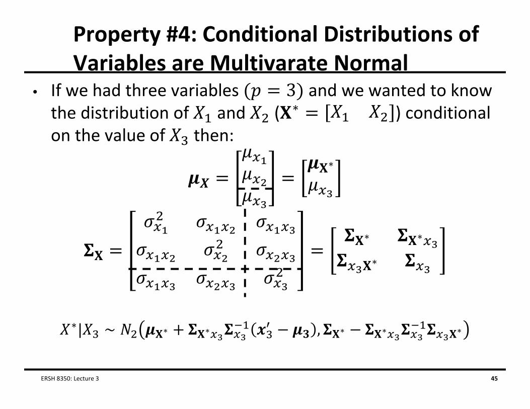
Property #4: Conditional Distributions of Variables are Multivarate Normal

• If we had three variables and we wanted to know the distribution of and ( ∗ ) conditional on the value of then:

∗

∗ ∗

∗

∗| ∼ ∗ ∗ , ∗ ∗ ∗


Sampling Distributions of MVN Statistics

• Just like in univariate statistics, there is a multivariate central limit theorem

If the set of observations on variables is multivariate normal or not:• The distribution of the mean vector is:

• The distribution of (covariance matrix) is Wishart (a multivariate chi‐square) with degrees of freedom


The Wishart Distribution

• The Wishart distribution is a multivariate chi‐square distribution

Input: S (model predicted covariance matrix)…Output: Likelihood value

Fixed: (sample value of covariance matrix)

• In statistics, it appears whenever: Data are assumed multivariate normal Only covariance matrix‐based inferences are needed

Mean vector ignored Mainly: Initial ML factor analysis and structural equation modeling


Sufficient Statistics

• The sample estimates and are called sufficient statistics All of the information contained in the data can be summarized by these two statistics alone No data is needed for analysis – only these statistics

• Only true when: Data truly follow a multivariate normal distribution No missing data are present


ASSESSING MULTIVARIATE NORMALITY


Assessing Multivariate Normality of Data

• A large number of statistical methods rely upon the assumption data follow a multivariate normal distribution Data “should” be multivariate normal then

• Methods exist for getting a rough picture of whether or not data are multivariate normal I will highlight a graphical method using the Q‐Q plot

• In reality: Determining exact distribution of data is difficult if not impossible

Methods that assume multivariate normality are fairly robust to small deviations from that assumption


Re‐examining the Multivariate Normal Distribution

• The multivariate normal distribution density is:

• The term in the exponent gives a scalar number that represents the squared “statistical” distance of a person’s observed variables to the mean Mahalanobis distance squared Distance contribution for each variable is standardized

• is distributed We now have a way we can construct a Q‐Q plot for assessing

multivariate normality


Q‐Q Plot for Multivariate Normality

• A Q‐Q Plot for multivariate normality is built by:1. Calculating using the sample

estimated mean vector and covariance matrix2. Ordering the from smallest to largest across all

observations3. Calculating the quantiles of each data point4. Looking up the quantiles of each data point using a

distribution (df = # of variables)5. Plotting the data against the value predicted by the

theoretical statistical distribution


Good News: SAS Macro for Assessing Multivariate Normality

• Although the process of assessing multivariate normality sounds tedious, our friends at SAS have simplified things considerably MULTNORM Macro available at: http://support.sas.com/kb/24/983.html

• The MULTNORM macro evaluates both univariate and multivariate using a set of hypothesis tests and plots The hypothesis tests can be difficult to use: very sensitive to violations of normality

The Q‐Q plots are better Big question: how much deviation is too much? Typical answer (from practice): doesn’t matter (no one checks)


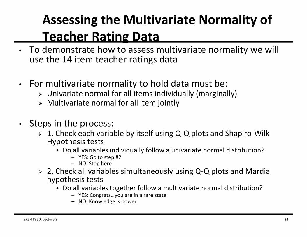
Assessing the Multivariate Normality of Teacher Rating Data

• To demonstrate how to assess multivariate normality we will use the 14 item teacher ratings data

• For multivariate normality to hold data must be: Univariate normal for all items individually (marginally) Multivariate normal for all item jointly

• Steps in the process: 1. Check each variable by itself using Q‐Q plots and Shapiro‐Wilk

Hypothesis tests Do all variables individually follow a univariate normal distribution?

– YES: Go to step #2– NO: Stop here

2. Check all variables simultaneously using Q‐Q plots and Mardiahypothesis tests Do all variables together follow a multivariate normal distribution?

– YES: Congrats…you are in a rare state– NO: Knowledge is power


Hypothesis Tests

• Shipiro‐Wilk univariate hypothesis test: : Data are univariate normal : Data are not univariate normal

• Based on these results: since univariate normality does not hold, multivariate normality cannot hold (we will continue on anyway)

• Mardia/Henze‐Zirkler Multivariate hypothesis test: : Data are multivariate normal : Data are not multivariate normal

Univariate Tests

Multivariate Tests


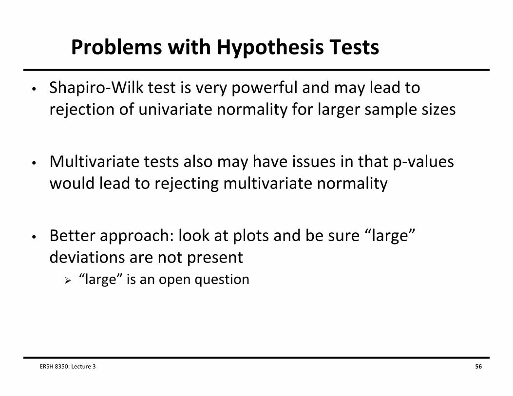
Problems with Hypothesis Tests

• Shapiro‐Wilk test is very powerful and may lead to rejection of univariate normality for larger sample sizes

• Multivariate tests also may have issues in that p‐values would lead to rejecting multivariate normality

• Better approach: look at plots and be sure “large” deviations are not present “large” is an open question


Univariate Plots


Item 13

Item 15Item 14

Item 12

Percent

Percent

Percent

Percent

Multivariate Q‐Q Plot of Squared Mahalanobis Distance


Checking Normality Again: Height and Weight Data

• Let’s now check for multivariate normality of our height and weight data from the beginning of class:

• Univariate tests: P‐values are large :: univariate normality likely for both variables

• Multivariate tests: P‐values large for Mardia tests, small for Henze‐Zirkler

• Conclusion from tests: likely multivariate normal


Graphical Inspection


When and Why to Check Normality• Good news: most methods are fairly robust to violations of

normality For homework we will have to check this assumption

• Methods taught in class where normality should be checked: Missing data imputation (unconditional data) Linear mixed models (conditional data ‐ residuals) Exploratory Factor Analysis (unconditional data) Confirmatory Factor Analysis (unconditional data) Structural Equation Modeling (unconditional and conditional data) Mixture models assuming normality (conditional data)

• If normality does not hold: Check your data for input errors (i.e., 99 = missing) Plot every variable – visualization is the most important thing Do not “clean” your data Use a model with a different link function, if possible (generalized model)


WRAPPING UP


Concluding Remarks• The univariate and multivariate normal distributions serve as

the backbone of the most frequently used statistical procedures They are very robust and very useful

• Understanding their form and function will help you learn about a whole host of statistical routines immediately This course is essentially a course based in normal distributions

• Inspecting normality is a tricky thing More often than not, data will not be normal More often than not, no one will check (don’t ask, don’t tell)

• Next week: linear models in matrices, repeated measures ANOVA, Multivariate ANOVA Classical statistics – described as a background for modern methods


univariate and multivariate statistical distributions · pdf filebivariate statistics ......

Documents