unitsand dimensions - publishing.cdlib.org
TRANSCRIPT

CHAPTERX11
Statics and Kinematics
. . . . . . . . . . . . . . . . . . . . . . . . . . . . . . . . . . . . . . . . . . . . . . . . . . . . . . . . . . . . . . . . . . . . . . . . . . . . . . . . . . . . . . . . . . . . . . . . . . . . . . . . . .
STATICS
Unitsand Dimensions
In the preceding chapters, different units have been introducedwithout strict definitions, but now it is necessary to define both unitsand dimensions. The word “dimension” in the English language is usedwith two different meanings. In everyday language, the term “ dimen-sions of an object” refers to the size of the object, but in physics “ dimen-sions*’ mean the fundamental categories by means of which physicalbodies, properties, or processes are described. In mechanics and hydro-dynamics, these fundamental dimensions are mass, length, and time,denoted by M, L, and T. When using the word “ dimension” in thissense, no indication of numerical magnitude is implied, but the concept isemphasized that any physical characteristic or property can be describedin terms of certain categories, the dimensions. This will be clarified byexamples on p. 402.
FUNDAMENTALUNITS. In physics the generally accepted units ofmass, length, and time are gram, centimeter, and second; that is, quanti-ties are expressed in the centimeter-gram-second (c.g.s.) system. Inoceanography, it is not always practicable to retain these units, because,in order to avoid using large numerical values, it is convenient to measuredepth, for instance, in meters and not in centimeters. Similarly, it isoften practical to use one metric ton as a unit of massinstead of one gram.The second is retained as the unit of time. A system of units based onmeter, ton, and second (the m.t.s. system) was introduced by V. Bjerknesand different collaborators (1910). Compared to the c.g.s. system thenew units are 1 m = 102cm, 1 metric ton = 106 g, 1 see = 1 sec. Forthermal processes, the fundamental unit, l“C, should be added.
Unfortunately, it is not practical to use even the m.t.s. system con-sistently. In several cases it is of advantage to adhere to the c.g.s.system in order to make resultsreadily comparable with laboratory resultsthat are expressed in such units, or because the numerical values aremore conveniently handled in the c.g.s. system. When measuring hori-
400

STATICS AND KINEMATICS 401
zontal distances, on the other hand, it is preferable to use larger unitssuch as kilometers, statute miles, or nautical miles. In’ oceanographyit is therefore always necessary to indicate the units in which any quan-tity is measured.
DERIVEDUNITS. Units in mechanics other than mass, 114,length, L,and time, T, can be expressed by the three dimensions, M, L, and T,and by the unit values adopted for these dimensions. Thus, velocityhas the dimension length divided by time, which is written as LT-l andis expressedin centimetersper second or in meters per second. Velocity,of course, can be expressed in many other units, such m nautical milesper hour (knots), or miles per day, but the dimensions remain unaltered.Acceleration is the time change of a velocity and has the dimensionsLT-2. Force is mass times acceleration and has dimensions ikfLT-~.
Table 60 shows the dimensions of a number of the terms that will beused. Several of the terms in the table have the same dimensions, butthe concepts o? which the terms are based differ. Work, for instance,is defined as force times distance, whereas kinetic energy is defined asmass times the square of a velocity, but work and kinetic energy bothhave the dimensions iWL2T-2. Similarly, one and the same term can bedefined differently, depending upon the concepts that are introduced.Pressure,for instance, can be defined as work per unit volume, ML2T–2L–3= NL-’T-Z, but is more often defined as force per unit area, MLT-2L–2= ~L-lj77-2.
TABLE 60‘-T” DIMENSIONSAND UNITS OF TERMS USEDIN MECHANICS ‘
Term
Fcmdwnmtal unitMesaLensithTim%
DerivedunitVelooityAooeler&ionAugular velocityMomentumForcelmpuIseWorkKinetic energyActivity (power)DemitySpeci6c volumePrecsureGravity potentialDynamio viscasityKinematic visccaityDiffusion
Dimen- IJnit in c.g.s. system I Unit in m.t.s. 8yatemaion
M g metrio ton - 106 g
L cm meter = 10S omT 8ec seo
LT-1 cm/8ec m/see = 100 cm/8ecLT-, om/see~ m,laecq = 100 em/secST-1 I[eae l/8ecML T-l g em/8ec ton m/see = 10$ g om/seclWLT-~ g om/sec~ = 1dyne ton m/se@ = 108 dynesML T-l g cm/8ec ton m/see = 10$ g cm/8eeJ.fL%T-Z ~ ~m*/~ec9 = 1 ~rg ton m9/see* = 1 kilojoule3.f&2T-2 g ~ma/8ec% = 1 ~~g tan m2/sec~ = 1 kilojouleML%T-8 g cm2/sec~ = erg/see ton m2/see* = 1 kilowatt~L-8 g/cm$ tOn/m8 = g/cm8Jf-1L8 ~m8/g ~8/t*n = ~@/g
ML-IT-* g/cm/secZ = dyne/em2 ton/m/aec2 = 1 oentibarLIT-2 ~m%/*e& ~2/Eee9 ~ 1 dyna~i~ deoimeter
bfL-IT-X g/Cm/8eC tOn/m/sec = 10$ g/cm/seeL%T-1 ~m2/*ea @/~ec = 104 ~m2/8ec
L2T-1 ~ml/g$e ~2/ee~ = 104 ~m2/@~
In any equation of physics, all terms must have the same dimensions,or, applied to mechanics, in all terms the exponents of the fundamental

402 STATICS AND KINEMATICS
dimensions, M, L, and l’, must be the same. It is inaccurate, forinstance, to state that the acceleration of a body is equal to the sum of theforces acting on a body, because acceleration has dimensions LT-2,whereas force has dimensions ik?LT-2. The correct statement is thatthe acceleration of a body is equal to the sum of the forces per unitmassacting on a body. An example of a correct statement is the expres-sion for the pressure exerted by a column of water of constant density,p, and of height, h, at a locality where the acceleration of gravity is g:
p = Pgh..
In this case the dimensions on both sides of the equality sign are
Some of the constants that appear in the equations of physics havedimensions, and their numerical values will therefore depend upon theparticular units that have been assigned to the fundamental dimensions,whereas other constants have no dimensions and are therefore independ-ent of the system of units. Density has dimensions ML-3, but the den-sity of pure water at 4° has the numerical value 1 (one) only if the unitsof mass and length are selected in a special manner (grams and centi-meters or metric tons and meters). On the other hand, the specific .gravity, which is the density of a body relative to the density of purewater at 4°, has no dimensions (ML–$/ML–3) and is therefore expressedby the same number, regardlessof the system of units that is employed.
The Fieldsof Gravity, Pressure,and Mass
LEVELSURFACES.Coordinate surfaces of equal geometric depthbelow the ideal sea surface are useful when considering geometricalfeatures, but in problems of statics or dynamics that involve considera-tion of the acting forces, they are not always satisfactory. Because thegravitational force represents one of the most important of the aotingforces, it is convenient to use as coordinate surfaces the level surfaces,defined as surfaces that are everywhere normal to the force of gravitg. Itwill presently be shown that these surfaces do not coincide with surfacesof equal geometric depth.
It follows from the definition of level surfaces that, if no forces otherthan gravitational are acting, a mass can be moved along a level surfacewithout expenditure of work and that the amount of work expended orgained by moving a unit mass from one surface to another is independentof the path taken.
The amount of work, W, required for moving a unit mass a distance,h, along the plumb line is
W = gh,

STATICS ANO KINEMATICS 403
where g is the acceleration of gravity. Work per unit mass has dlmen-siona L2Z’-2, and the numerical value depend~ therefore only on theunits used for length and time. When the length is measured in metersand the time in seconds, the unit of work per unit mass is called a d~namicdecimeter (Bjerknes and different collaborators, 1910).
In the following, the sea surface will be considered a level surface.The work required or gained in moving a unit,mass from sea level to apoint above or below sea level is called the gravity potential, and in them.t.s. system the unit of gravity potential is thus one dynamic decimeter.
The practical unit of the gravity potential is the dynamic meter,for which the symbol D is used. When dealing with the sea the verticalaxis is taken as positive downward. The geopotential of a level surfaceat the geometrical depth, z, is therefore, in dynamic meters,
The geometrical depth in meters of a givenhand, is
z =. 10s
D ~ dD.09
(XII, 1)
level surface, on the other
(XII, 2)
The acceleration of gravity varies with latitude and depth, and thegeometrical distance between s$andard level surfaces therefore varieswith the coordinates. At the North Pole the geometrical depth of the1000-dynamic-meter surface is 1017.0 m, but at the Equator the depthis 1022.3m, because g is greater at the Poles than at the Equator. Thus,level surfaces and surfaces of equal geometric depth do not coincide. ~Level surfaces slope relative to the surfaces of equal geometric depth,and therefore a component of the acceleration of gravity acts alongsurfaces of equal geometrical depth.
The topography of the sea bottom is represented by means of iso-baths—that is, linesof equal geometrical depth—but it could be presentedequally well by means of lines of equal geopotential. The contour lines Iwould then represent the lines of intersection between the level surfacesand the irregularsurface of the bottom. These contours would no longerbe at equal geometric distances, and hence would differ from the usualtopographic chart, but their characteristicswould be that the amount ofwork needed for moving a given mass from one contour to another wouldbe constant. They would also represent the new coast lines if the sealevel were lowered without alterations of the topographic features of thebottom, provided the new sea level would assume perfect hydrostaticequilibrium and adjust itself normal to the gravitational force.
Any scalar field can similarly be represented by means of a seriesof topographic charts of equiscalar surfaces in which the contour lines

404 STATICS AND KINEMATICS
represent the lines of intersection of the level surfaces with the equi-scalar surface. Charts of this character will be called geopotential topo-graphic charts, or charts of geopotentiul topography, in contrast totopographic charts in which the contour lines represent the lines alongwhich the depth of the surface under consideration is constant.
THE FIELDOF GRAVITY. The fact that gravity is the resultant oftwo forces, the attraction of the earth and the centrifugal force due to theearth’s rotation, need not be considered, and it is sufficient to definegravity as the force that is derived empirically by pendulum observations.Furthermore, it is not necessary to take into account the minor irregularvariations of gravity that detailed surveys reveal, but it is enough to makeuse of the ‘(normal” value, in meters per second per second, which at sealevel can be represented as a function of the latitude, p, by Helmert’sformula:
go = 9.80616(1 – 0.002644 COS 2P + 0.000007 COS.22qJ).
Thus, the normal value at the poles is 9.83205, and at the Equator it is9.78027. ‘I’he normal value of g increases with depth, according to theformula
9 = go + 2.202 x 10–%.
From formula (XII, 1) one obtains in dynamic meters the geopotentialthat corresponds to a given depth, z:
D = (&z + 0.1101 x 1O-%P,
or from (XII, 2) the depth corresponding to a given value of D:
z = # D – 0.1168 X 10⁻⁶D2.
In the first approximation,
D = 0.98z and z = 1.02D,
meaning that the numbers which represent the depth in meters deviateonly by about 2 per cent from the numbers which represent the geo-potential in dynamic meters. Extensive use will be made of this numeri-cal agreement between the two units, but it must always be borne inmind that a dynamic meter is a measure of work per unit mass, and nota measureof length. The conversion factors, 0.98 and 1.02, are thereforenot pure numbers, but the former has the dimensionsLT-2 and the latterhas the dimensionsL–lTZ.
The field of gravity can be completely described by means of a setof equipotential surfacesgravity potential. These
corresponding to standard intervals of theare at equal distances if the geopotential is
STATICS AND KINEMATICS 405
used as the vertical coordinate, but, if geometric. depth is used, thedistance between the eqnipotential surfaces varies. If the field isrepresented by equipotential surfaces at intervals of one dynamicdecimeter, it follows from the definition of these surfaces that the numeri-cal value of the acceleration of gravity is the reciprocal of the geometricthickness in meters of the unit sheets.
TEE FIELDOF PRESSVRE. The distribution of pressure in the seacan be determined by means of the equation of static equilibrium:
dp = iipe,a,Pgdz. (XII, 3)
Here, k is a numerical factor that depends on the units used, and pg,o,P isthe density of the water (p. 56).
The hydrostatic equation will be discussed further in connection withthe equations of motion (p. 440). At this time it is enough to emphasizethat, as far as conditions in the ocean are concerned, the equation, forall practical purposes, is exact.
Introducing the geopotential expressed in dynamic meters as thevertical coordinate, one has 10dD = gdz. When the pressureis measuredin decibars (defined by 1 bar = 106 dynes per square centimeter), thefactor k becomes equal to }io, and equation (XII, 3) is reduced to
dp = P8,ff,pd~? or dD = a.,@ip,
where a,,~,Pis the specific volume.Because p.,~,P and a~,~,gdiffer little from unity, a difference in pressure
is expressed in decibars by nearly the same number that expresses thedifference in geopotential in dynamic meters, or the difference in geo-metric depth in meters. Approximately,
pl – p2=I)1-D2==z1-.z2.
The pressure field can be completely described by means of a systemof isobaric surfaces. Using the geopotential as the vertical coordinate,one can present the pressure distribution by a series of charts showingisobars at standard level surfaces or by a series of charts showing thegeopotential topography of standard isobaric surfaces. In meteorology,the former manner of representation is generally used on weather maps,in which the pressure distribution at sea level is represented by isobars.In oceanography, on the other hand, it has been found practical torepresent the geopotential topography of isobaric surfaces.
The pressuregradientis defined by
Gdp=—— ,dn
where n is dhected normal to the isobaric surfaces (p. 156). The pressure

406 STATICS AND KINEMATICS
gradient has the character of a force per unit volume, because pressurehaethe dimensions of a force per unit area. The dimension of a pressure isML-IT-Z = M.L!f’-2 X L-2, and the dimension of a pressure gradient isML-2 T-2 = MLT-2 X L-8. Multiplying the pressure gradient by thespecific volume, lf-1L3, one obtains a force per unit mass of dimensionsLT-2.
The pressure gradient has two principal components: the vertical,directed normal to the level surfaces, and the horizontal, directed parallelto the level surfaces. When static equilibrium exists, the vertical com-ponent, expressed as force per unit mass, is balanced by the accelerationof gravity. This is the statement which is expressed mathematicallyby means of the equation of hydrostatic equilibrium. In a restingsystem the horizontal component of the pressuregradient is not balancedby any other force, and therefore the existence of a horizontal pressuregradient indicates that the system is not at rest or cannot remain at rest.The horizontal pressure gradients, therefore, although extremely small,are all-important to the state of motion, whereas the vertical are insig-nificant in this respect.
It is evident that no motion due to pressure distribution exists orcan develop if the isobaric surfaces coincide with level surfaces. Insuch a state of perfect hydrostatic equilibrium the horizontal pressuregradient vanishes. Such a state would be present if the atmosphericpressure, acting on the sea surface, were constant, if the sea surfacecoincided with the ideal sea level and if the density of the water dependedon pressure only. None of these conditions is fulfilled. The isobaricsurfaces are generally inclined relative to the level surfaces, and hori-zontal pressuregradients are present, forming a field of internal force.
This field of force can also be defined by considering the slopesof isobaric surfaces instead of the horizontal pressure gradients. Bydefinition the pressure gradient along an isobaric surface is zero, but, ifthis surface does not coincide with a level surface, a component of theacceleration of gravity acts along the isobaric surface and will tend toset the water in motion, or must be balanced by other forces if a steadystate of motion is reached. The internal field of force can therefore berepresentedalso by means of the component of the acceleration of gravityalong isobaric surfaces (p. 440).
Regardless of the definition of the field of force that is associatedwith the pressure distribution, for a complete description of this fieldone must know the absolute isobars at level surfaces or the absotutegeopotential contour lines of isobaric surfaces. These demands cannotpossibly be met. One reason is that measurements of geopotentialdistances of isobaric surfaces must be made from the actual sea surface,the topography of which is unknown. It will be shown that all one cando is to determine the pressurefield that would be present if the pressure
STATICS AND Kinematics 407
distribution depended only upon the distribution of mass in the sea.This part of the total pressure field will be called the rekdiw jieid ojpreswwe,but it cannot be too strongly emphasised that the toW $eld ojpressure is composed of this relative field and, in addltiori, a field thatis maintained.by external forces such as atmospheric pressure and wind.
In order to illustrate this point a fresh-water lake will be consideredwhich is so small that horizontal differences in atmospheric pressurecan be disregarded and the acceleration of gravity can be consideredconstant. Let it first be assumed that the water is homogeneous,meaning that the density is independent of the coordinates. In thiscase, the distance between any two isobaric surfaces is expressed by theequation
Ah = ~ Ap. (XII, 4)
This equation simply states that the geometrical distance between iso-baric surfaces is constant, and it defines completely the internal field ofpressure. The total field of pressure depends, however, upon theconfiguration of the free surface of the lake. If no wind blows and ifno stress is thus exerted on the free surface of the lake, perfect hydro-static equilibrium exists, the free surface is a level surface, and, similarly,all other isobaric surfaces coincide with level surfaces. On the otherhand, if a wind blows across the lake, the equilibrium will be disturbed,the water level will be lowered at one end of the lake, and water will bepiled up against the other end. The free surface will still be an isobaricsurface, but it will now be inclined relative to a level surface. Therela$i~efield of pressure, however, will remain unaltered as representedby equation (XII, 4), meaning that all other isobaric surfaces will havethe same geometric shape as that of the free surface.
One might continue and introduce a number of layers of differentdensity, and one would find that the same reasoning would be applicable.The method is therefore also applicable when one deals with a liquidwit~ln which the density changes continually with depth. By means ofobservations of the density at different depths, one can derive the relativefield of pressureand can represent this by means of the topography of theisobaric surfaces re.ktive to some arbitrarily or purposely selected isobaricsurface. The relative field of force can be derived from the slopes of theisobaric surface relative to the selected reference surface, but, in orderto find the absolute field of pressure and the corresponding absolutefield of force, it is necessary to determine the absolute shape of oneisobaric surface.
These considerations have been set forth in great detail becauseit is essential to be fully aware of the difference between the absolutefield of pressureand the relative field of pressure,and to know what typesof data are needed in order to determine each of these fields.

408 STATICS AND KINEMATICS
TKE l?IE~DOF MASS. The field of mass in the ocean is generallydescribed by means of the specific volume as expressed by (p. 57)
The field of the specific volume can be considered as composed of twofields, the field of a,,,o,p and the field of &
The former field is of a simple character. The surfaces of ~85,0,p
coincide with the isobaric surfaces, the deviations of which from levelsurfaces are so small that for practical purposes the surfaces of CYS5,0,P
can be considered as coinciding with level surfaces or with surfaces ofequal geometric depth. The field of CW,,O,Pcan therefore be fully describedby means of tables giving CY35,0,P as a function of pressure and giving theaverage relationships between pressure, geopotential and geometricdepths. Since this field can be considered a constant one, the field ofmass is completely described by means of the anomaly of the specificvolume, d, the determination of which was discussed on p. 58.
The field of mass can be represented by means of the topography ofanomaly surfaces or by means of horizontal charts or vertical sectionsin which curves of 8 = constant are entered. The latter method is themost common. It should always be borne in mind, however, that thespecific volume @ situis equal to the sum of the standard specific volume,a35,o,p,at the pressure in situ and the anomaly, ~.
THE RELATIVEFIELDOF PRESSURE.It is impossible to determinethe relative field of pressurein the sea by direct observations, using sometype of pressure gauge, because an error of only 0.1 m in the depth of apressure gauge below the sea surface would introduce errors greaterthan the horizontal differences that should be established. If the fieldof mass is known, however, the internal field of pressure can be deter-mined from the equation of static equilibrium in one of the forms
dp = pdD or dD = adp.
In oceanography the latter form has been found to be the more practical,but all reasoning applies equally well to results deduced from the former.
Integration of the latter form gives
Because (x*,$fp= a35,fJ,* + d,
one can write
(D, –1
‘* ddp,D,), i- AD = ~’ wi,o,pdp + p, (XII, 6)
where (D, – D2)* = ~ cwo,pdp
and is called the standard geopotential distance between the isobaric

STATICS AND KUWMATICS 409
surfaces PI and pz, and where
AD=~c3dp (XII, 7)
is oalled the anomaly of the geopotential distance between the isobaricsurfaces PI and pz, or, abbreviated, the geopotentkl anomaly.
Equation (XII, 6) can be interpreted as expressing that the relativefield of pressure is composed of two fields: the standard field and thefierd of anomalies. The standard field can be determined once and forall, because the standard geopotential distance between isobaric surfacesrepresents the distance if the salinity of the sea water is constant at85 0/00 and the temperature is constant at O°C. The standard geo-potential distance decreaseswith increasing pressure,because the specificvolume decreases(density increases)with pressure,as isevident from table7H in Bjerknes (1910), according to which the standard geopotentialdistance between the isobaric surfaces O and 100 decibars is 97.242dynamic meters, whereas the corresponding distance between the 5000-and 5100-decibar surfaces is 95.153 dynamic meters.
The standard geopotential distance between any two standardisobaric surfaces is, on the other hand, independent of latitude, butthe geometric dwtance between isobaric surfaces varies with latitudebecause g varies.
Because in the standard field all isobaric surfaces are parallel relativeto each other, this standard field lacks a ~e.?ai%vefield of horizontal force.The relative field of force, which is associated with the dhtribution ofmass, is completely described by the field of the geopotential anomalies.It follows that a chart showing the topography of one isobaric surfacerelative to another by means of the geopotential anomalies is equivalentto a chart showing the actual geopotential topography of one isobaricsurface relative to another. The practical determination of the relativefield of pressure is therefore reduced to computation and representationof the geopotential anomalies, but the absolute pressure field can befound oidy if one can determine independently the absolute topographyof ,one isobaric surface.
In order to evaluate equation (XII, 7), it is necessary to know theanomaly, 3, as a function of absolute pressure. The anomaly is com-puted from observations of temperature and salinity, but oceanographicobservations give information about the temperature and the salinity atknown geometrical depths below the actual sea surface, and not at knownpressures. Thk difficulty can fortunately be overcome by means of anartificial substitution, because at any given depth the numerical value ofthe absolute pressure expressed in decibars is nearly the same as thenumerical value of the depth expressed in meters, as is evident from thefollowing corresponding values:
410 STATICS AND KINEMATICS
Standardseapressure (decibars). . . . . . . . . . . 1000 2000 3000 4000 5000 6000Approximate geometric depth (m). ., . . . . . , . 990 1975 2956 3933 4906 5875
Thus, the numerical values of geometric depth deviate only 1 or 2 percent from the numerical values of the standard pressure at that depth.This agreement is not accidental, but has been brought about by theselection of the practical unit of pressure, the decibar.
It follows that the temperature at a pressure of 1000 decibars isnearly equal to the temperature at a geometric depth of 990 m, or $hetemperature at the pressure of 6000 decibars is nearly equal to’ thetemperature at a depth of 5875 m. The vertical temperature gradientsin the ocean are small, especially at great depths, and therefore no seriouserror is introduced if, instead of using the temperature at 990 m whencomputing 6, one makes use of the temperature at 1000 m, and so on.The difference between anomalies for neighboring stations will be evenless affected by this procedure, because within a limited area the verticaltemperature gradients will be similar. The introduced error will benearly the same at both stations, and the difference will be an error ofabsolutely negligible amount, In pr%ctice one can therefore consider .the numbers that represent the geometric depth in meters as representingabaolute pressure in deuibar$. If the depth in meters at which eitherdirectly observed or interpolated values of temperature and salinityare available is interpreted as representing pressure in decibars, one cancompute, by means of the tables in the appendix, the anomaly of specificvolume at the given pressure. By multiplying the average anomaly ofspecific volume between two pressures by the difference in pressure indecibars (which is considered equal to the difference in depth in meters),one obtains the geopotential anomaly of the isobaric sheet in questionexpressed in dynamic meters. By adding these geopotential anomalies,one can find the correspondhg anomaly between any two given pres-sures. An example of a complete computation is given in table 61.
Certain simple relationships between the field of pressure and thefield of mass can be derived by means of the equations for equiscalarsurfaces (p, 155) and the hydrostatic equation. In a vertical pfofile theisobars and the isopycnak are defined by
The inclinations of the isobars and isopycnals are therefore
ap/8x .ipap/a~— .
= - @Z%’ ‘p = - ap/dz
By means of the hydrostatic equation

STATICS AND KINEMATICS 411
TABLE 61
EXAMPLEOF COMPUTATIONOF ANOMALIESOF DYNAMIC DEPTH(StationE. W. ScrippsI-8. Lat. 32°57’N, .ong. 122°07’W. February17, 1938)
Metersordeoibars
o... . . . . .lo . . . . . . . .25.., . . . . .50. . . . . . . .75. . . . . . . .
100 . . . . . . . .150. . . . . . . .200. . . . . . . .250. . . . . . .300. . . . . . . .400. . . . . . . .500. . . . . . . .600. . . . . . . .800. . . . . . . .
1000. . . . . . .1200. . . . . . . .1400. . . . . . .1600. . . . . . . .1800. . . . . . .2000. . . . . . .3000. . . . . . .4000. . . . . . .
remp.(“c)
.—
14.2213.72
.71
.359.96
.388.82
.48‘ .307.87
.076.145.514.653.99
.52
.072.69
.37
.131.62
.50
$lalin-ity
(O/.O)
33.25.24 I.24.30.57.84.98
34.09.16.20.20.26.35.42.44.52.54.56.59.64.68.7-0
qt
4.81.91.91
5.03.86
6.17.37.51.59.69.80.97
7.12.28.36.48.54,59.64.69.76.81
106A,,$
315.0305.5305.5294.2215.2185.7166.5153.5145,9136.4125.9109.895.680.472.961.555.851.146.341.635.030.2
-
.0%,,p
-0.1–0.2-0.3-0.3-0.3-0.4–0.5–0,6-0.7-0.8-1.0–l. !2–1.4–1.0-1,0–1.0-1,1-1.4–1.7
10%*<P
0.30.71.31.62.02.93.74.65.26,47.27.98.99.8
10.310.810.910.810.611.714.1
,066
315306306296?17187169157150141132116103888270666156514543
ADAD (dynamic
meter)
!.0310.0459
.0310
.0769.0752 .~521.0641.0505
.2162
:0890.2667
.0815 .3557
.0768.4372
.0728 :;:;
.1365.7233.1240 .~73
.1095 .9568
:y~: 1.1478
;;5& ; ::;:8
1.606: ;;; 1.733
1.850‘ 1070 1.957:g;: 2.437
2.877
one obtains
gpip = – ap/ax,
From the two latter equations it follows that
:(p’a=++!
s(@P)’2 – (P~P)l = 12 ‘4 g“
If the density distribution is representedby means of unit sheets (p. 156),the integral on the right-hand side can be evaluated
(P’M2 – (P’Ml = UP2 – PA (XII, 8)
where Z@means the average inclination of unit sheets. The isob$%icsurface PI lies above the surface p%,because the vertical axis is positivedownward. The inclination of the upper isobaric surface relative to thelower, iP,_P2,therefore, when an average value of the density is intro-
412 STATICS AND KINEMATICS
duced, is
~P1-P2 = -;, ~’.
P
Using the specific volume anomaly and making the specific volume equalto unity, one obtains approximately
k-m = —:$(61 — 32). (XII, 9)
Because 6 decreases with depth, & – & is positive, and the inclinationof one isobaric surface relative to another is of opposite sign to theinclination of the 6 surfaces (p. 449). This rule permits a rapid estimateof the relative inclinations of isobaric surface in a section in which thefield of mass has been represented by ~ curves.
Profiles of isobaric surfaces based on the data from a seriesof stationsin a section must evidently be in agreement with the inclination of the 6curves, as shown in a section and based on the same data, but this obviousrule often receives little or no attention.
RELATIVE GEOPOTENTIALTOPOGRAPHYOF ISOBARICSURFACES.If simultaneous observations of the vertical distribution of temperatureand salinity were available from a number of oceanographic stationswithin a given area, the relative pressuredistribution at the time of theobservations could be represented by a series of charts showing the geo-potential topography of standard isobaric surfaces relative to onearbitrarily or purposely selected reference surface. From the precedingit is evident that these topographies are completely representedby meansof the geopotential anomalies.
In practice, simultaneous observations are not available, but inmany instances it is permissible to assume that the time changes of thepressuredistribution are so small that observations taken within a givenperiod may be considered simultaneous. The smaller the area, theshorter must be the time interval within which the observations aremade. Figs. 110, p. 454 and 204, p. 726, represent examples of geo-potential topographies. The conclusions as to currents which can bebased on such charts will be considered later.
Charts of geopotential topographies can be prepared in two differentways. By the common method, the anomalies of a given surface relativeto the selected reference surface are plotted on a chart and isolines aredrawn, following the general rules for presenting scalar quantities. Inthk manner, relative topographies of a series of isobaric surfaces can beprepared, but the method has the disadvantage that each topographyis prepared separately.
By the other method a series of charts of relative topographies isprepared stepwise, taking advantage of the fact that the anomaly of geo-potential thickness of an isobaric sheet is proportional to the average

STATICS AND KINEMATICS 413
“ specific volume anomaly, ~, in the.ieobmio sheet. Thus, if the thicknessof the isobaric sheet is 100 decibars, AD&lOO= 100& Consequently,curves of 1003 represent the topography of the surface p = PI — 100relative to the surface p = PI, and one can proceed as follows: The topog-raphy of the surface p. – 200, where p. is the selected reference surface$is constructed by means of curves of equal values of the specific volumeanomaly in the sheet p, to p, -100. The topography of the surfacePe – 200 relative to the surface p, - 100 is constructed by means of thespecific volume anomalies in the sheet p, — 100 to p, — 200, and bygraphical addition of these two charts (V. Bjerkmw and collaborators,1911) the topography of the surface p. -200 relative to the surfacep, is found. This process can be repeated, and by successive construc-tions of charts and specific volume anomaliesand by graphical additions,the entire fields of mass and pressure can be represented.
This method is widely used in meteorology, but is not commonlyemployed in oceanography because, for the most part, the differentsystems of curves are so nearly parallel to each other that graphicaladdition is cumbersome. The method is occasionally useful, however,and has the advantage of showing clearly the relationship between thedistribution of mass and the distribution of pressure. It especiallybrings out the geometrical feature that the isohypses of the isobaricsurfacesretaintheir form when passingfrom one isobaricsurfaceto anotheronly if the anomaly curves are of the same form as the isohypses. Thischaracteristic of the field is of great importance to the dynamics of thesystem.
CHARACTEROF THETOTALFIELDOF PRESSWRE.From the abovediscussion it is evident that, in the absenceof a relative field of pressure,isosteric and isobaric surfaces must coincide. Therefore, if for somereason one isobaric surface, say the free surface, deviates from a levelsurface, then all isobaric and isosteric surfaces must deviate in a similarmanner. Assume that one isobaric surface in the disturbed conditionlies at a distance Ah cm below the position in undisturbed conditions.Then all other isobaric surfaces along the same vertical are also dis-placed the distance Ah from their undisturbed position. The distanceM. is positive downward because the positive z axis points downward.Call the pressure at a given depth at undisturbed conditions PO. Thenthe pressure at disturbed conditions is P6 = PO – flp, where Ap = gpAhand where the displacement Ah can be considered as being due to adeficit or an excess of mass in the water column under consideration.
The above considerations are equally valid if a relative field ofpressure exists. The absolute distribution of pressure can always becompletely determined from the equation
pt = PO– gpAh,

414 STATICS AND KINEMATICS
and would therefore be fully known if one could determineAh, the verticaldisplacement of the isobaric surfaces due to excess or deficit of mass inthe column under consideration, An added horizontal field of force ispresent when this vertical displacement varies from one locality toanother, in which case the absolute isobaric surfaces slope in relation tothe isobaric surfaces of the relative field. The added field can be calledthe slope field, and this analysis thus leads to the result that the totalfield of pressure is composed of the internal field and the slope field.This distinction is helpful when discussing the character of the currents.
Significanceof atSurfaces
The density of sea water at atmospheric pressure, expressed asat = (P.wxo– 1) X 103, is often computed and represented in horizontalcharts or vertical sections. It is therefore necessary to study the sig-nificance of u~surfaces, and in order to do so the following problemwill be considered: Can water masses be exchanged between differentplaces in the ocean space without altering the distribution of mass?
The same problem will first‘be considered for the atmosphere, assum-ing that this is a perfect, dry gas. In such an atmosphere the potentialtemperature means the temperature which the air would have if it werebrought by an adiabatic process to a standard pressure. The potentialtemperature, d, is
where $ is the temperature at the pressurep, PO is the standard pressure,and x = 1.4053 is the ratio of the two specific heatsof an ideal gas (c@/c, ).In a dry atmosphere in which the temperaturevaries in spaceand in whichthe vertical gradient differs from the gradient at adiabatic equilibrium,it is always possible to define surfaces of equal potential temperature.One characteristic of these surfaces is that along such a surface air massescan be interchanged without altering the distribution of temperatureand pressureand, thus, without altering the distribution of mass.
Consider two air masses, one of temperature & at pressure PI, andone of temperature 82 at pressure pz. If both have the same potentialtemperature, it follows that
or

STATICS AND KIWMATICS 415
The latter equations tell that if the air mass originally characterizedby &, PZ is brought adiabatically to pressure PI, its temperature hasbeen changed to 81, and, similarly, thst the air mass which originallywas characterized by @l, PI attains the temperature % if brought topressurepz. Thus, no alteration of the dktribution of mass is made byan exchange, andsuch anexchange hasnoinfluence either onthe poten-tial energy of the system or on the entropy of the system. In an idealgas the surfacesof potential temperature are therefore isentropic surfaces.
With regard to the ocean, the question to be considered is whethersurfaces of similar characteristics can be found there. Let one watermass at tho geopotential depth D1 be characterized by salinity SI andtemperature 01, and another water mass at geopotential depth Lh becharacterized by salinity S2 and temperature & The densities in situof these small water masses can then be expressed as CTSl,~Aand U8*,d@y
Now consider that the mass at the geopotential depth D1 is movedadiabatically to the geopotential depth Q. During this process thetemperature of the water mass will change adiabatically from t% to 91. .and the density in Mu w1ll be a,,,e,,~z. Moving the other water massadiabatically from Dz to DI will change its temperature from % to &If the two water masses are interchanged, the conditions
‘81, @i,% = %,$%%, ‘8%,%% = a8%,kDl (XII, 10)
must both be fulfilled if the distribution of mass shall remain unaltered,These conditions can be fulfilled, however, only in the trivial case thatS1 = S2, ?91 G &f and DI = D2. This is best illustrated by a numericalexample. Assume the values
s, = 36.01 O/oo, & = 13.73”, DI = 200 dyn meters.Sz = 34.60 0/00, ~, = 8.10”, Di = 700 dyn meters.
These values represent conditions encountered in the Atlantic Ocean, butat a distance of about 50° of latitude.
The adiabatic change in temperature between the geopotential depthsof 200 and 700 dyn meters is 0.09°, and thus L%= 13.82, f?z= 8.01.By means of the Hydrographic Tables of Bjerknes and collaborators, onefinds
~a,.Qt.D* = 30.24, U82,&z,Dt = 30.24, dHference = 0.00.gal,%% = 27.97, ~*2,e%,I)i= 27.92, difference = 0.05.
Thus, the conditions (XII, 10) are not both fulfllled and the two watermasses cannot be interchanged without altering the distribution of mass.
It should also be observed that the mixing of two water masses thatare at the same depth and are of the same density in w-k, but of differenttemperatures and salinities, produces water of a higher density. If,at D = 700 dyn meters, equal parts of water S1 = 36.01 0/00,& = 13.82°,

416 STATICS AND KINEMATICS
and & = 34.60 0/00,02 = 8.10°, respectively, are mixed, the resultingmix-ture will have a salinity S = 35.305 0/00, and a temperature & = 10.96°.The density in situof the two water masseswas identical (a,,~,~= 30.24),but the resulting mixture has a higher density, 30.29. Similarly, ifequal parts of the water masses S1 = 36.01 O/.O,01 = 13.73°, D1 = 200dyn meters, and St = 34.60 0/00,& = 8.01°, and D.2= 200 dyn metersare mixed, the density in m“tuof the mixture will be 27.98, although thedensities of the two water masseswere 27.97 and 27,92, respectively.
This discussion leads to the conclusion that in the ocean no surfacesexist along which interchange or mixing of water masses can take placewithout altering the distribution of mass and thus altering the potentialenergy and the entropy of the system (except in the trivial case thatisohaline and isothermal surfaces coincide with level surfaces). Theremust exist, however, a set of surfaces of such character that the changeof potential energy and entropy is at a minimum if interchange andmixing takes place along these surfaces. It is impossible to determinethe shape of these surfaces, but the at surfaces approximately satisfy theconditions. In the preceding example, which represents very extremeconditions, the two water masses were lying nearly on the same atsurface (a~l= 27.05, u,, = 26.97).
Thus, in the ocean, the u, surfaces can be considered as being nearlyequivalent to the isentropic surfaces in a dry atmosphere, and the c~surfaces may therefore be called quasi-isentropic surfaces. The nameimplies only that interchange or mixing of water massesalong atsurfacesbrings about small changes of the potential energy and of the entropy ofthe body of water.
Stability
The change in a vertical direction of a, is nearly proportional to thevertical dabitit~of the system. Assume that a water mass is displacedvertically upward from the geopotential depth D2 to the geopotentialdepth D1. The difference between the density of this mass and thesurrounding water (see p. 57) will then be
where Aa~,AS, and A@ represent the variations of at, S and @ betweenthe geopotentials Dl to D2, and where A19representsthe adiabatic changeof temperature. The water mass will evidently remain at rest in the newsurroundings if Ap = O; it will sink back to its original place if Ap ispositive, because it is then heavier than the surroundings; and will rise ifAp is negative, because it is then lighter than the surroundings. Theacceleration of the mass will be proportional to AP/p. The reasoningremains unaltered if we introduce geometric depths instead of geo-potential. If the acceleration due to displacement along the short

STATICSAND KfNEMATICS
vertical diatxmceAZ is proportional to AP/p, thento displacement along a vertical distance of unitportional to Ap/pAz. IIesselberg (1918) has called
417
the acceleration duelength must be pro-the term
(XII, 12)
the” stability.” Omitting the factor l/p, which differs little from unity,one obtains, by means of equation (XII, 11),
(YG,DdSE=10-8~+— —
; aeO,~da ap d6——— .dS dz ao dz dfi dz
(XII, 13)
where d@/dz is the adiabatic change of temperature per unit length.This term is small, and, because thee terms and the vertical gradients ofsalinity and temperature also are small, it follows that, approximately,
E’ = 10-$ ~.
.TABLE 62
STABILITY AT MICHAEL tYAR8 STATIONNO. 44(Lat.28°37’N,Long.19°0SW. May% 1910)
Depth (m)Temp.(“c)
19.2.31.34.24
18.65.24
17.5016.4514.5213.0811.8510.809.09
, Sol7.276.404.522.342.432.49
?&nity(“/00)
36.87.85.83.79.79.’78.56.40,02
35.77.64.54.39.37,42.35.15
84.92.60.90
26.43.38.35.34.49.58.61.73.33.99
27.13.25.43.58.74.30.87.86.87.87
o . . . . . . . . . . . . . . . . . . . . .10. . . . . . . . . . . . . . . . . . . . .25. . . . . . . . . . . . . . . . . . . . .50. . . . . . . . . . . . . . . . . . . . .75. . . . . . . . . . . . . . . . . . . . .
100, . . . . . . . . . . . . . . . . . . . .150. . . . . . . . . . . . . . . . . . . . .200. . . . . . . . . . . . . . . . . . . . .300. . . . . . . . . . . . . . . . . . . . .400. . . . . . . . . . . . . . . . . . . . .500. . . . . . . . . . . . . . . . . . . . .600. . . . . . . . . . . . . . . . . . . . .800. . . . . . . . . . . . . . . . . . . . .
1000. . . . . . . . . . . . . . . . . . . . .1200. . . . . . . . . . . . . . . . . . . . .1400. . . . . . . . . . . . . . . . . . . . .2W . . . . . . . . . . . . . . . . . . . . .mom. . . . . . . . . . . . . . . . . . .4000. . . . . . . . . . . . . . . . . . . . .5000. . . . . . . . . . . . . . . . . . . .
Hesselberg and Sverdrup (1914-15) have published tables by meansof which the terms of equation (XII, 13) are found, and give an example.based on observations in the Atlantic Ocean on May, 1910,in lat. 28”37’N,long. 19”08’W (Helland-Hansen, 1930). Thw example is reproduced in
–440– 150-1361039034
27016012015013010089S4483911.27.61.3
(XII, 14)
O’(cb/dz)
–400–200-40
%!60
24015011014012090758030
:;
:’ “

418 STATICSAND KINEMATICS
table 62, in which the exact values of the stability are given under theheading 108ZI,and the approximate values, obtained by means of equation(XII, 14), under the heading 10$du,/dz. The two values agree fairlywell down to a depth of 1400 m. The negative values above 50 m indi-cate instability,
Hesselberg and Sverdrup have also computed the order of magnitudeof the different terms in equation (XII, 13) and have shown that duJdzis an accurate expression of the stability down to a depth of 100 m, butthat between 100 and 2000 m the terms containing emay have to be con-sidered, and that below 2000 m all terms are important. The followingpractical Wles can be given:
1. Above 100 m the stability is accurately expressed by means of10-3 duJciz.
2. Below 100m the magnitude of the other termsof the exact equation(XII, 13) should be examined if the numerical value of 10-B dut/dz is lessthan 40 X 10-8.
The stability can also be expressed in a manner that is useful whenconsidering the stability of the deep water:
(XII, 15)
If the salinity does not vary with depth (dS/dzin the deep water,
E()
.3? f!?-;.W dz
= O), as is often the case
(XII, 16)
Of the quantities in thk equation, t@/tM is negative, d6/dz is positive,and d$/dz is negative if the temperature decreases with depth, butpositive if the temperature increases. The stratification will always bestable if the temperature decreases with depth or increasesmore slowlythan the adiabatic, but indifferent equilibrium exists if dO/dz = d(?/dz,and instability is found if dO/dz > df?/dz.
KINEMATICS
Vector Fields
A vector field can be completely represented by means of three setsof charts, one of which shows the scalar field of the magnitude of thevector and two of which show the direction of the vector in horizontal andvertical planes. It can also be fully described by means of three sets ofscalar fields representingthe components of the vector along the principalcoordinate axes (V. Bj erknes and Wf erent collaborators, 1911). Inoceanography, one is concerned mainly with vectors that are horizontal,such as velocity of ocean currents-that is, two-dimensional vectors.

STATICS ANQ KllW4ATfCS 419
These can be completely represented by means of two sets of charts,or one chart with two sets of curves--vector lines, which at all points givethe direction of the vector, and equisoalar curves, which give the mag-nitude of the vector, Fig. 95 shows a schematic example of an arbitrarytwo-dimensional vector field that is represented by means of vectors ofindicated direction and magnitude and by means of vector lines andequiscslm curves of magnitude. ‘
Fig.95. Representationof a two-dimensionalvectorfieldby vectorsof indioateddirectionandmagnitudeandby vectorlinesandequismlarcurves.
Vector lines cannot intersect except at singular points or lines, wherethe magnitude of the vector is zero. Vector lines cannot begin or endwithh the vector field except at singular points, and vector lines arecontiriuous.
The simplest and most important singularities in a two-dimensionalvector field are shown in fig. 96: These are (1) points of divergence(fig. 96A and C) or convergence (fig. 96B and D), at which an infinitenumber of vector lines meet; (2) neutral poirtte, at which two or morevector lines intersect (the example in fig. 9613shows a neutral point of thefirst order in which two vector lines intersect—-that is, a hyperbolicpoint); and (3) lines of divergence (fig. 96F) or convergence (fig. 96G),from which an infinite number of vector lines diverge asymptoticallyor to which an infinite number of vector lines converge asymptotioalIy.

420 STATICS AND KINEMATICS-
The significance of these singularities in the field of motion will beexplained below.
It is not necessary to enter upon all the characteristics of vectorfields or upon all the vector operations that can be performed, but twoimportant vector operations must be mentioned.
.
F G
Fig. 96. Singularities in a two-dimensional vector field. A and C, points ofdivergence; B and D, points of convergence; E, neutral point of first order (hyperbolicpoint); F, line of convergence; and #, line of divergence.
Assume that a vector A has the components A., AV, and A$. Thescalar quantity
is called the di~ergenceof the vector.

STATICS AND KINEMATICS 421
The vector which has the components
is called the curl, or the vorticity, of the vector A. Divergence andvorticity of fields of velocity or momentum have definite physicalinterpretations.
Two representations of a vector that varies in space and time willalso be mentioned. A vector that has been observed at a given localityduring a certain time interval can be represented by means of a centrazvectordiagram (fig. 97). In this diagram, all vectors are plotted from thesame point, and the time of ob-servation is indicated at eachvector. Occasionally the endpoints of the vector are joined by
~: fit
a curve on which the time of ob- t:”servation is indicated and the Fig. 97. Time wuistion of a veotorvectors themselves are omitted. representedby a centralvector diagramThis form of representation is (te.f$and a progressivevector diagram
commonly used when dealing(rigM).
with periodic currents such as tidal currents. A central vector diagramis also used extensively in pilot charts to indicate the frequency of windsfrom given directions. In this case the direction of thewind is shown byan arrow, and the frequency of wind from that direction is shown by thelength of the arrow.
If it can be assumed that the observations were made in a uniformvector field, a progressive vector diagram is useful. Thk diagram isconstructed by plotting the second vector from the end point of the first,and so on (fig. 97). When dealing with velocity, one can compute thedisplacement due to the average velocity over a short interval of time.When these displacements are plotted in a progressive vector diagram,the resulting curve will show the trajectoryof a particle if the velocityfield is of such uniformity that the observed velocity can be consideredrepresentative of the velocities in the neighborhood of the place ofobservation. The vector that can be drawn from the beginning of thefirst vector to the. end of the last shows the total displacement in theentire time interval, and this displacement, divided by the time interval,is the averagevelocity for the period.

422 STATICS AND KINEMATICS
The Field of Motion andthe Equationof Continuity
THE FIELD OF MOTION. Among vector fields the field of motion isof special importance. Several of the characteristics of the field ofmotion can be dealt with without considering the forces which havebrought about or which maintain the motion, and these characteristicsform the subject of kinematics.
The velocity of a particle relative to a given coordinate system isdefined as v = dr/dt, where dr is an element of length in the directionin which the particle moves. In a rectangular coordinate system thevelocity has the components
The velocity field can be completely described by the Lagrange orby the Euler method. In the Lagrange method the coordinates of allmoving particles are represented as functions of time and of a threefoldmultitude of parameters that together characterize all the movingparticles. From this representation the velocity of each particle, and,thus, the velocity field, can be derived at any time.
The more convenient method by Euler will be employed in the follow-ing. This method assumes that the velocity of all particles of the fluidhas been defined. On this assumption the velocity field is completelydescribed if the components of the velocity can be representedas functionsof the coordinates and of time:
v. = j’.(z,y,z,t),% = AAWAO,v. = j’z(z,y,z,t).
The characteristic difference between the two methods is thatLagrange’s method focuses attention on the paths taken by all individualparticles, whereas Euler’s method focuses attention on the velocity ateach point in the coordinate space. In Euler’s method it is necessary,however, to consider the motion of the individual particles in order tofind the acceleration. After a time dt, a particle that, at the time f,was at the point (z,y,.z) and had the velocity components ~O(Z,y,Z,t),andso on, will be at the point (z + dq y + dy, z + dz), and will have thevelocity components jz(x + dx, y+ d~, z + dz, t + dt), and so on.Expanding in Taylor’s series, one obtains
j’.(x + dm, y + dy,, z + dz,, t + dtJ
The change in velocity in the time dt—--thatis, the acceleration of the
STATICS AND KINEMATICS 423
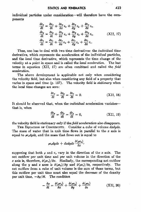
individual particles under consideration-will therefore have the comp-onents
dv= 8V= au= ~V= av=2E=7F+ZV’+ZV”+ W’”dv,
%’+~v=+$v, +$vs,Z=at(XII, 17)
do. au.at +
av.—=—dt
gv. + 3VW+Z V,,a~
Thus, one has to deal with two time derivatives: the individual timederivative, which represents the acceleration of the individual particles,and the local time derivative, which represents the time change of thevelocity at a point in space and is called the local acceleration. The lastterms in equation (XII, 17) are often combined and called the $ekiacceleration.
The above development is applicable not only when consideringthe velocity field, but also when considering any field of a property thatvaries in space and time (p. 157). The velocity field is stakionarg whenthe 100altime changes are zero:
~z=~_av. ~at at -z=”
(XII, 18)
It should be observed that, when the individual acceleration vanisheethat is, when
(XII, 19)
the velocity field is stationary only if the j%id acceleration also disappears.THE EQUATION OF CONTINUITY. Consider a cube of volume dzdgdz.
The mass of water that in unit time flows in parallel to the z axis isequal to pv=dydz, and the mass that flows out is equal to
supposing that both p and VZvary in the direction of the x axis. Thenet outflow per unit time and per unit volume in the direction of thez axis is, therefore, d(pvJ/&u Eknihwly, the corresponding net outflowalong the y and z axes is 6’(pvJ/dy and’6@vJ/tkj respectively. Thenet outflow from a cube of unit volume isthe sum of these terms, butthis outflow per unit time must also equal the decrease of the densityper unit time, -+/at. The condition
(XII, 20)

424 STATICS AND .KINEMATICS
must therefore always be fulfilled in order to maintain the continuity ofthe system. This fundamentally important equation is called the equa-tion of continuity. It tells that the local 10.ssoj mass, represented by– c?p/&2 equals the divergence of the specific momentum (p. 420).
Now:
By means of equation (XII, 17), therefore,
1 dp 1 da au= + 4VU.—— =.— .— -&Y + $“p dt adt ax+ (XII, 21)
The term on the left-hand side represents the rate of expansion of themoving element. In this form the equation of continuity states thatthe rate of expantion of the moving element equals the divergenceof theve$ocitg.
The equation of continuity is not valid in the above format a bound-ary surface because no out-or inflow can take place there. In a directionnormal to a boundary a particle in that surface must move at the samevelocity as the surface itself. If the surface is rigid, no componentnormal to the surface exists and the velocity must be directed parallelto the surface. The condition
dn‘“ = -a’
(XII, 22)
where n is directed normal to the boundary surface and dn/dt is thevelocity of the boundary surface in this direction, representsthe kinematicboundary condition,which at the boundary takes the place of the equationof continuity.
APPLICATION OF THE EQUATION OF CONTINUITY. At the sea surfacethe kinematic boundary condition must be fulfilled. Designating thevertical displacement of the sea surface relative to a certain level ofequilibrium by q, and taking this distance positive downward, becausethe positive z axis is directed downward, one obtains
aq.‘“0 = z’
that is, the vertical velocity at the sea surface is equal to the time changeof the elevation of the sea surface. If the sea surface remainsstationary,one has V,,O= O. If the bottom is level, one has, similarly, V#,h= O,where h is the depth to the bottom.
With stationary distribution of mass (dP/at = O) the equation ofcontinuity is reduced to
?*+~@!k)+?$?#. o.ax ay (XII, 23)

STATICS AND. KINEMATICS 425
The total transport of mass through a vertical surface of unit widthreaching from the surface to the bottom has the components
Multiplying equation (XII, 23) by dz and integrating from the surfaceto the bottom, one obtains
dMs dMu—+—as au + (P%)o – (PVJO= o.
Here, vz,h = O, and at stationary sea level vZ,O= O. ‘Thus, the equationis reduced to
divlkl=o, (XII, 24)
or, when the sea level remains daiionarg, the transport between the surfaceand t~e bottiom is jree of divergence.
When dealing with conditions near the surface, one can consider thedensity as constant and can introduce average values of the velocitycomponents % and OYwithin a top layer of thickness H. With thesesimplifications, one obtains, putting V,,O = O,
If His small enough, the average velocity will not diiler much from thesurface velocity. Since a negative vertical velocity’ represents anascending motion, and a positive vertical velocity representsa descendingmotion, equation (XII, 25) states that at a small distance below thesurface ascending motion is encountered if the surface currents arediverging, and descending if the surface currents are converging. Thisis an obvious conclusion, because, with diverging surface currents,water is carried away from the area of divergence and must be replacedby water that rises from some depth below the surface, and vice versa.Thus, conclusions as to vertical motion can be based on charts showingthe surface currents.
For this ‘purpose, it is of advantage to write the divergence of a two-dimensional vector field in a different form:
v dAndivv=~+— —
.dl An dl ‘(XII, 26)
where dl is an element of length in the.direction of flow and where Anrepresentsthe distance between neighboring streamlines. If the velocityis constant along the stream lines (dv/dt = 0)-,the flow is divergent whenthe distance between the stream lines increases (dAn/dl > O), andconvergent when the distance decreases (dAn/dl < O). When, on the

426 STATICS AND KINEMATICS
other hand, the distance between the stream lines remains constant(dAn/dl = O), the divergence depends only upon the change of velocityalong the streamlines. Increasingvelocity (do/di > O)meansdivergenceaccompanied by ascending motion below the surface if this surfaceremains stationary, and decreasing velocity (6’v/dl < O) means con-vergence associated with descending motion below the surface.
The equation of continuity is applicable not only to the field of massbut also to the field of a dissolved substance that is not influenced bybiological activity. Let the mass of the substance per unit mass ofwater bes. Multiplying the equation of continuity bys and integratingfrom the surface to bottom, one obtains, if the vertical velocity at thesurface is zero,
!#+div P=O,
where
Under stationary conditions the local time change is zero, and one has
div P = O, div Al = O.
These equations have already been used in simplified form in orderto compute the relation between inflow and outflow of basins (p. 147).Other simplifications have been introduced by Knudsen, Witting, and
Fig. 98. Trajectories(fulldrawnlines)and streamlines(dashedlines)in a pro-gressivesurfacewave.
Gehrke (Kriimmel, 1911, p. 509-512).
STREAM LINES AND TRAJEC-TORIU3. The vector lines show-ing the direction of currents ata given time are called the streamlines, or the lines o.f jtow. Thepaths followed by the movingwater particles, on the other hand,are called the trajectories of the
particles. Stream lines and trajectories are identical only when themotion is stationary, in which case the stream lines of the velocity fieldremain unaltered in time, and a particle remains on the same streamline.
The general difference between stream lines and trajectories canbe illustrated by considering the type of motion in a traveling surfacewave. The solid lines with arrows in fig. 98 show the streamlines in across section of a surface wave that is supposed to move from left to right,passing the point A. When the crest of the wave passes A, the motionof the water particlesat A is in the direction of progress,but with decreas~

STATICS AND KtNEMATK23 427
ing velocities downward. At the troughs of the wave, at b and e, themotion is in the opposite dhwction. Between A rmdb there is, therefore,a divergence with descending motion, and between A and e there is aconvergence with aseendhg motion. The surface will therefore sinkat c and rise at d, meaning that the wave will travel from left to right.When the point c reaches A, there will be no horizontal motion of thewater, but as b passesA the motion will be reversed. Thus, the patternof stream lines moves from left to right with the velocity at which thewave proceeds.
It is supposed that the speed at which the wave travels is muchgreater than the velocity of the single water particles that take part inthe wave motion. On this assumption a water particle that originallywas located below A will never be much removed from this vertical andwill return after one wave period to its original position. The trajectoriesof such particles in this case are circles, the diameters of which decreasewith increasing distance from the surface, w shown in the figure. It isevident that the trajectories bear no similarity to the stream Iines.
Representationsof the Field of Motion in the Sea
Trajectories of the surface water m~ses of the ocean can be deter-mined by following the drift of floating bodies that are carried by thecurrents. It is necessary, however, to exercise considerable care wheninterpreting the available information about drift of bodies, becauseoften the wind has carried the body through the water. Furthermore, inmost cases, only the end points of the trajectory are known—that is, thelocalities where the drift commenced and ended. Results of drift-bottleexperiments present an example of incomplete inforination as to trajec-tories. As a rule, drift bottles are recovered on beaches, and a recon-struction of the paths taken by the bottles from the places at which theywere released may be very hypothetical. The reconstruction may beaided by additional information in the form of knowledge of distributionof surface temperatures and salinities that are related to the currents,or by information obtained from drift bottles that have been picked upat sea. Systematic drift-bottle experiments have been conducted,especially in coastal areas that are of importance to fisheries.
iik!reawzlivum of the actual surface or subsurface currents must bebased upon a very large number of direct current measurements, Wherethe velocity is not stationary, simultaneous observations are required.Direct measurementsof subsurface currents must be made from anchoredvessels, but this procedure is so diilicult that no simultrmeousmeasure-ments that can be used for preparing charts of observed subsurfacecurrents for any area are available,
Numerous observations of surface currents, on the other hand, havebeen derived from ships’ logs. Assume that the position of the vessel at
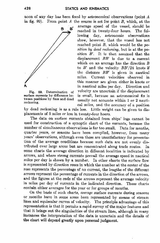
428 STATICS AND KINEMATICS
noon of any day has been fixed by astronomical observations (point Ain fig. 99). From point A the course is set for point 1?, whkh, at the
A
Fig. 99. Determination ofsurface currents by difference be-tween positions by fixes and deadreckoning.
average speed of the vessel, should bereached in twenty-four hours. The fol-lowing day, astronomic observationsshow, however, that the vessel has notreached point B, which would be the po-sition by dead reckoning, but is at the po-sition B’. It is then assumed that thedisplacement BB’ is due to a currentwhich on an average has the direction Bto B’ and the velocity BB’/24 knots ifthe distance BB’ is given in nauticalmiles. Current velocities observed inthis manner are given either in knots orin nautical miles per day. Direction andvelocity are uncertain if the displacementis small, because an astronomical fix isusually not accurate within 1 or 2 nauti-cal miles, and the accuracv of a ~osition
by dead reckoning is as a rule less. Little weight can b; give; to dis-placements of 5 miles or less in twenty-four hours.
The data on surface currents obtained from ships’ logs cannot beused for construction of a synoptic chart of the currents, because thenumber of simultaneousobservations is far too small. Data for months,quarter years, or seasons have been compiled, however, from manyyears’ observations, although even these are unsatisfactory for presenta-tion of the average conditions because such data are not evenly dis-tributed over large areas but are concentrated along trade routes. Insome charts the average direction in different localities is indicated byarrows, and where strong currents prevail the average speed in nauticalmiles per day is shown by a number. In other charts the surface flowis representedby direction roses in which the number at the center of therose represents the percentage of no current, the lengths of the differentarrows representthe percentage of currents in the direction of the arrows,and the figures at the ends of the arrows represent the average velocityin miles per day of currents in the indicated direction. These chartscontain either averages for the year or for groups of months.
On the basis of such charts, averagesurface currents during seasonsor ,montbs have in some areas been represented by means of streamlines and equiscalar curves of velocity. The principle advantage of thisrepresentation is that it permits a rapid survey of the major features andthat it brings out the singularitiesof the stream lines, although in manyinstances the interpretation of the data is uncertain and the details ofthe chart will depend greatly upon personal judgment.

STATICS AND KINEMATICS 429
In drawing these stream lines it is necessary to follow the rulesconcerning vector lines (p. 419). The stream lines cannot intersect,but an infinite number of stream lines can meet in a point of convergenceor divergence or can approach asymptotically a line of convergence ordiverge asymptotically from a line of divergence.
y / :
\
/
,.ids 4.W 4s J-r 5.5” w
l?k. 100. Streamhues of the surfacecurrentsoff southeasternAfricain JUIY(after Willimzik).
As an example, stream lines of the surface flow in July off southeastAfrica and to the south and southeast of Madagascar are shown in fig. 100.The figure is based on a chart by Willimzik (1929), but a number of thestream lines in the original chart have been omitted for the sake ofsimplification. In the chart a number of the characteristic singularitiesof a vector field are shown. Three hyperbolic points marked A appear,four points of convergence marked B are seen, and a number of lines ofconvergence marked C and lines of divergence marked D are present.The stream lines do not everywhere run parallel to the coast, and therepresentation involves the assumption of vertical motion at the coast,where the horizonttilvelocity, however, must vanish.

430 STATICSAND KINEMATICS
The most conspicuous feature is the continuous line of convergencethat to the southwest of Madagascar curves south and then runs west,following lat. 35°S. At this line of convergence, the Subtropical Con-vergence, which can be traced across the entire Indian Ocean and has itscounterpart in other oceans, descending motion must take place. Simi-larly, descending motion must be present at the other lines of conver-gence, at the points of convergence, and at the east coast of Madagascar,whereas ascending motion must be present along the lines of divergenceand along the west coast of Madagascar, where the surface watersflow away from the coast. Velocity curves have been omitted, for whichreason the conclusions as to vertical motion remain incomplete (seep. 425). Near the coasts, eddies or countercurrents are indicated, andthese phenomena often represent characteristic features of the flow andremain unaltered during long periods.
As has already been stated, representationsof surface flow by meansof stream lines have been prepared in a few cases only. As a rule, thesurface currents are shown by means of arrows. In some instances therepresentation is based on ships’ observation of currents, but in othercases the surface flow has been derived from observed distribution oftemperature and salinity, perhaps taking results of drift-bottle experi-ments into account. The velocity of the currents may not be indicatedor may be shown by added numerals, or by the thickness of the arrows.No uniform system has been adopted (see Defant, 1929), because theavailable data are of such different kinds that in ‘each individual casea form of representation must be selected which presents the availableinformation in the most satisfactory manner. Other examples of surfaceflow will be given in the section dealing with the currents in specific areas.
Bibliography
Bjerknes, V., and different collaborators. 1910. Dynamic meteorology andhydrography. Pt. I. Statics. CarnegieInst. Washington,Pub. no. 88,146pp. -t tables. 1910.
1911. Dynamicmeteorologyand hydrography. Pt, II. Kine-matics. CarnegieInst. Washington,Pub. no. 88, 175pp., 1911.
Defant,A. 1929. DynamischeOzeanographle, NaturwissenschaftlicheMono-graphlenundLehrbucher,Bd. 9, HI, 222 pp,, 1929. Berlin,
Helland-Hansen,B. 1930. Physicaloceanographyand meteorology. MichaelSarsNorthAtlanticDeep-SeaExped.,1910,Rept. Sci.Results,v. 1, art, 2,217pp., 1930.
Hesselberg,Th. 1918. Uber die StabiEtatsverh<nissebei vertikalenVer-schlebungenin der Atmosphiireund im Meer. Ann. d. Hydr. u. Mar.Meteor.,p, 118-29, 1918.
Hesselberg,Th., and H. U. Sverdrup. 1915. Die StabMtiitsverhtiMnissedesSeewassersbei vertikalen Verschiebungen. Bergens Museums Aarbok1914–15,No. 15, 16 pp., 1915.
WMimzik,M. 1929. Die Stromungenim subtropischenKonvergenzgebletdesIndkchen Ozeans. Berlin, Universitat.Institut f. Meereskunde,Vertiff.,N. F., A. Geogr,-naturwiss.Reihe,Heft 14,27 pp., 1929.