United States Imports

Michael WilliamsKevin Crider

Andreas LindalJim HuangJuan Shan

Agenda

Introduction

Data

Modeling

Results

Conclusion

Introduction

Introduction

Data

Modeling

Results

Conclusion

US is ranked as No. 4 globalized county in the world

Import is a key index to measure globalization

Source: ChristianSarkar.com

Introduction

Introduction

Data

Modeling

Results

Conclusion

1

2

3

4

5

6

60 65 70 75 80 85 90 95 00 05

RATIO of Import to GDP

%

Year

The ratio of US import good/service to GDP is increasing

United States is transforming from a closed economy to an open environment

IMPORTS Trend

Introduction

Data

Modeling

Results

Conclusion

0

200

400

600

800

60 65 70 75 80 85 90 95 00 05

IMPORTS

Billions of Dollars

Year

Trace shows increasing trend with time

IMPORTS Histogram

Introduction

Data

Modeling

Results

Conclusion

0

10

20

30

40

50

60

0 100 200 300 400 500 600 700 800

Series: IMPORTSSample 1960:1 2007:4Observations 192

Mean 179.1564Median 107.6990Maximum 781.4380Minimum 5.599000Std. Dev. 195.8587Skewness 1.307456Kurtosis 3.967978

Jarque-Bera 62.19795Probability 0.000000

IMPORTS Correlogram

Introduction

Data

Modeling

Results

Conclusion

Big spike at lag one on PACF

Suspicion of unit root

IMPORTS ADF Test

Introduction

Data

Modeling

Results

Conclusion

Time series is not stationary

Needs prewhitening before we could apply Box Jenkins modeling

Introduction

Data

Modeling

Results

Conclusion

High Kurtosis discards normality

More needs to be done to explain the trend

0

20

40

60

80

-30 -20 -10 0 10 20 30 40

Series: DIMPORTSSample 1960:2 2007:4Observations 191

Mean 4.059623Median 1.984000Maximum 44.81900Minimum -31.74500Std. Dev. 8.618069Skewness 1.007605Kurtosis 8.850218

Jarque-Bera 304.6937Probability 0.000000

DIMPORTS Histogram

Dickey-Fuller Test

Introduction

Data

Modeling

Results

Conclusion

Unit root test confirms stationarity

Regression can now be performed

DIMPORTS Correlogram

Introduction

Data

Modeling

Results

Conclusion

Spike at lag one and two in PACF

Structure indicates a possible AR(2)

AR Model Estimation

Introduction

Data

Modeling

Results

Conclusion

Both AR components are significant

High F-stat

Correlogram of AR Model

Introduction

Data

Modeling

Results

Conclusion

-40

-20

0

20

40-40

-20

0

20

40

60

65 70 75 80 85 90 95 00 05

Residual Actual Fitted

Correlogram looks orthogonal, but Q-stats are significant

ARCH Test Results

Introduction

Data

Modeling

Results

Conclusion

ARCH test indicates that ARCH term is needed in the model to account for conditional variance

ARCH Model

Estimation

Introduction

Data

Modeling

Results

Conclusion

Both ARCH terms and GARCH term turn out significant

ARCH Model Correlogram

Introduction

Data

Modeling

Results

Conclusion

Q-statistic stays inside confidence interval

Correlogram is orthogonal

Introduction

Data

Modeling

Results

Conclusion

ARCH Residual Histogram

0

5

10

15

20

25

30

-2 -1 0 1 2

Series: Standardized ResidualsSample 1960:4 2007:4Observations 189

Mean 0.177455Median 0.177076Maximum 2.395230Minimum -2.733968Std. Dev. 0.979940Skewness -0.340291Kurtosis 3.361821

Jarque-Bera 4.678593Probability 0.096395

Introduction

Data

Modeling

Results

Conclusion

Actual, Fitted, Residuals

-40

-20

0

20

40-40

-20

0

20

40

60

65 70 75 80 85 90 95 00 05

Residual Actual Fitted

Residuals graph indicates heteroskedasticity

Likely would be improved with VAR Model

Introduction

Data

Modeling

Results

Conclusion

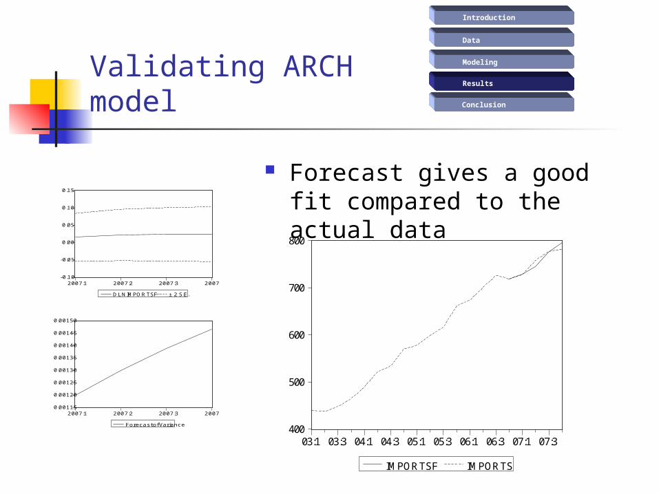
Forecast gives a good fit compared to the actual data

Validating ARCH model

400

500

600

700

800

03:1 03:3 04:1 04:3 05:1 05:3 06:1 06:3 07:1 07:3

IMPORTSF IMPORTS

-0.10

-0.05

0.00

0.05

0.10

0.15

2007:1 2007:2 2007:3 2007:4

D LN IMPOR TSF ± 2 S.E.

Forecas t: D LN IMPOR TSFAc tual: D LN IMPOR TSSample: 2007:1 2007:4Inc lude observations : 4

R oot Mean Squared Error 0.012921Mean Abs olute Error 0.009777Mean Abs . Perc ent Error 105.0272Theil Inequality C oeffic ient 0.278665 Bias Proportion 0.000075 Var ianc e Proportion 0.504202 C ovariance Proportion 0.495723

0.00115

0.00120

0.00125

0.00130

0.00135

0.00140

0.00145

0.00150

2007:1 2007:2 2007:3 2007:4

Forecas t of Variance

Introduction

Data

Modeling

Results

Conclusion2008 Forecast

-0.06

-0.04

-0.02

0.00

0.02

0.04

0.06

0.08

0.10

2008:1 2008:2 2008:3 2008:4

DLNIMPORTSF2 ± 2 S.E.

0.0006

0.0007

0.0008

0.0009

0.0010

0.0011

2008:1 2008:2 2008:3 2008:4

Forecast of Variance

300

400

500

600

700

800

900

1000

00 01 02 03 04 05 06 07 08

UPPERLOWER

IMPORTSF2IMPORTS

Introduction

Data

Modeling

Results

ConclusionConclusion

Questions?

US Imports should continue to grow faster than GDPPerhaps there are other techniques we could use in the future to address the correlation in our residuals