united states air force air force institute of … · preface this effort demonstrates a systems...
TRANSCRIPT
AFIT/EN/TR/97-02
UNITED STATES AIR FORCE
AIR FORCE INSTITUTE OF TECHNOLOGY
An Application of System Dynamics Analysis
to Ecosystem Management at the Poinsett
Weapons Range, Shaw AFB SC
M. Brennan P. Colborn
J. Goodbody T. Grady
S. Kearney L. Lilley
P. Marbas M. Shelley
D. Wise T. Wood
DEPARTMENT OF ENGINEERING AND ENVIRONMENTAL MANAGEMENT
GRADUATE SCHOOL OF ENGINEERING
December 1997
Approved for public release;
distribution unlimited
AFIT/ENV, 2950 P Street Wright Patterson AFB OH
45433-7765
DKCQt7AUTyIWSpECTBDl
PREFACE
This effort demonstrates a systems analysis approach toward addressing long term management strategies using the particular application of management of natural resources. The document is the final capstone course project report of students in the Air Force Institute of Technology's resident masters program in Engineering and Environmental Management. Most participating students are also using this technique in pursuit of their individual thesis research efforts in various technical and management areas and have explored applications of system dynamics modeling at the graduate level.
The attached application addresses specific challenges in ecosystem management related to the operation of the Poinsett Weapons Range maintained by Shaw AFB SC. Issues include long term management of forest systems for control of species composition and biodiversity as well as endangered species management concerns. Findings suggest near term management options which are expected to optimize long term conditions consistent with sustainable Air Force training operations. The report can be used as a reference for fundamental principles in natural resource and endangered species management, as a reference for management of long leaf pine stands and red cockaded woodpecker populations specifically, and, perhaps most importantly, as a reference for how the management tool of system dynamics simulation can be used to address a wide variety of issues surrounding management of complex systems, both natural as well economic and organizational.
Contributing AFIT graduate students:
Capt Mark Brennan (USMC) Capt Louis Lilley . Capt Phil Colborn (USMC) Capt Pat Marbas
Lt Jason Goodbody Capt Doug Wise Mr Ted Grady Capt Tim Wood Capt Scott Kearney
Faculty Advisor: Dr Mike Shelley
Special thanks to the very professional team of managers at Shaw AFB whose innovative and forward looking natural resources management program made this effort possible. Their enthusiastic support and contribution to this effort was greatly appreciated.
Shaw AFB personnel:
Mr Terry Madewell, Chief, Natural Resources Management Mr Stan Rogers, Wildlife and Environmental Impact Analysis Manager Ms Suzanne Shipper-Tayler, Endangered Species and Cultural Resources Manager

ENVR 775 Strategic Environmental Management
Team Project Final Report 02 Sep 97
Table of Contents
List of Figures
List of Tables
I. Introduction
Problem Statement Ecosystem Description Project Purpose Client Objectives
Formulation Testing Implementation
Page
4
7 7 9 9
Research Questions 10
II. Literature Review 11
Longleaf Pines J J Turkey Oaks J| Red-Cockaded Woodpeckers 1° Cavity Competitors 24 Cavity Trees
III. Methodology 29
Conceptualization 30
33 34
IV. Model Presentation 35
Tree Sector 35 Cavity Sector *1 Red-Cockaded Woodpecker Sector 44
Overall Model Interaction 50
V. Model Testing and Discussion 51
Baseline Output j|2 Validation Testing 53 Sensitivity Testing 55 Model Strengths and Weaknesses 67

VI. Alternative Management Scenarios and Recommendations 71
Catastrophic Events Management Scenarios Jz Recommendations iz
VII. Conclusions
Answers to Research Questions Suggestions for Further Study
Bibliography
Appendix A — Model Assumptions
Appendix B — Model Structure
Appendix C — Model Equations and Values
87
89
89 90
93
98
113
128

List of Figures
Figure Pa9e
1. Hypothesized Reference Mode 51
2. Baseline Output with Current Management Practices 52
3. Baseline Sensitivity Analysis Graph 56
4. Acceptable Cavities with Variation of Artificial Cavity Construction Rates 57
5. Acceptable Cavities with Variation of Initial Squirrel Population 58
6. Acceptable Cavities with Variation of Pioneering Rates 59
7. Acceptable Cavities with Variation of Opening Plate Construction Rates 60
8. Longleaf Pine with Variation of Artificial Cavity Construction Rates 61
9. RCW Population Sensitivity to Birth Rate 62
10. RCW Population with Variation of Relatedness Entity 64
11. RCW Population with Variation of Foraging Area per RCW 65
12. RCW Population with Variation of Artificial Translocation Rate 66
13. Baseline Management Scenario Graph 71
14. Hurricane Effects on Mature LLP 72
15. Hurricane Effects on Turkey Oak 73
16. Hurricane Effects on RCW Population 74
17. Southern Pine Beetle Effects on Mature LLP 75
18. Southern Pine Beetle Effects on Turkey Oak 76
19. Baseline Populations with No Management Practices 77
20. Effects of Mechanical Removal on Mature LLPs 78
21. Effects of Mechanical Removal on Turkey Oaks 79
22. LLP Densities with Varying Time Between Burns 80
23. Turkey Oak Densities with Varying Time Between Burns 80
24. Effects of Competitor Management on RCW Population 82
25. Effects of Artificial Cavity Construction on RCW Population 84
26. Effects of Translocation on RCW Population 86
27. Effects of Birth Rate on RCW Population 87

List of Tables
Table Pa9e
1. Longleaf Pine Mortality 15
2. Mortality Rates for the RCW 23
1. Introduction
Problem Statement. One of the more challenging missions for the
Environmental Flight at Shaw Air Force Base, North Carolina is the protection of the
endangered Red-Cockaded Woodpecker (Picoides Borealis) and the management of
the Poinsett Weapons Range ecosystem. Currently, the population trends of the Red-
Cockaded Woodpecker (RCW) within the Poinsett Weapons Range ecosystem have
the potential to negatively impact the base's primary mission of maintaining the highest
level of Air Force combat capability and readiness. Short term management efforts to
improve the ecosystem are resource intensive. The long-term effects of current
management practices on the ecosystem are not clearly understood. A long-term
sustainable approach to produce a stable ecosystem with minimum resource
expenditure is needed.
Ecosystem Description. The Poinsett Weapons Range is located in Sumter
County, South Carolina and is operated by the United States Air Force at Shaw Air
Force Base. Resources include 12,500 acres of forested areas which consist of slash
pine, longleaf pine, loblolly pine, and various hardwoods (Shaw AFB Natural Resources
Management Division, 1996:1). As of February of 1995, the range had nine known
active clusters (aggregate of cavity trees used by a RCW group) and eight known
inactive clusters (Shaw AFB, 1995). By 1997, the active clusters decreased to six while
the inactive clusters rose to ten respectively (Rogers, 1997). The Air Force is obligated
to manage the RCW under section 7 of the Endangered Species Act (ESA) and is
currently working with the U.S. Fish and Wildlife Service (USFWS) to proactively
manage the RCW population in accordance with the ESA requirements. Current
habitat management practices include: nesting habitat maintenance, foraging habitat
maintenance, burning, erosion control, timber harvesting, pine straw harvesting,
restoration and construction of cavities, cluster protection, augmentation/translocation,
surveys, and inspections and monitoring.
The RCW is a non-migratory species of woodpecker once common throughout
the pine forests of the Southeastern United States, preferring mature longleaf pine
savannahs (Jackson, 1994; U.S. Fish and Wildlife Service, 1985:1-88). The RCW
population has been significantly reduced due to habitat loss as a result of clearing of
the pine forests for agriculture and development. As a result, the RCW has been on
the Federal Endangered Species list since 1970. Even though there are six active
clusters at the Poinsett Range, only three breeding pairs with one helper per breeding
pair and three solitary males currently exist in the Poinsett Range habitat (Rogers,
1997).
The longleaf pine (Pinus palustris) is the primary tree used for excavation of
cavities by the RCW. The longleaf pine forests were once prevalent throughout the
Southeastern United States, stretching from South Carolina to Texas. Since then, fire
suppression, livestock, clear cutting, the lumber industry and other human influences,
have reduced the range of the longleaf pine significantly. A forest inventory conducted
for the Poinsett Range resulted in stands within the 6,098 acres of upland manageable
forest being designated as mostly longleaf (42% of stands) and slash pine (39%) (Shaw
AFB Natural Resources Management Division, 1996:2).
The health of the ecosystem for this project is primarily determined by the age
distribution and density of the longleaf pine stands. Such an LLP ecosystem is
hypothesized to be similar to that found in pre-colonial eras and is optimal for RCW
sustainability.
Project Purpose. To address the concerns associated with the RCW and its
habitat and to explore the implications of various management practices, the project
team will employ strategic environmental management and a system dynamics
approach to simulate ecosystem processes over a long time period. The purpose of
this effort is to gain a better understanding of the ecosystem entities and
interrelationships found in a RCW and longleaf pine habitat and to identify the
influences driving system behavior and management practices most effective in
establishing a long-term stable low-maintenance ecosystem. Improved understanding
of these relationships will allow the Shaw AFB Environmental Flight to better manage
the range in a sustainable manner.
Client Primary Objectives. The client's primary objectives will influence the entire
modeling process. Their objectives (Shelley, 1997) for the project include:
1. Avoiding mission stoppage from regulatory action concerned with RCW issues.
2. Ensuring biodiversity, stability, resilience, etc., consistent with relatively undisturbed ecosystems of the same type in the vicinity.
3. Improving RCW habitat (old longleaf pine) in compliance with the RCW Plan.
4. Achieve sustainable natural resource income to fund the program.

Research Questions. To keep the entire project focused and to ensure the
client's objectives are met, specific research questions are addressed. These
questions include:
1. How is the number of RCW clusters affected by environmental factors and management practices?
2. What are the impacts on the longleaf pine ecosystem viability if habitat management is driven by RCW population goals?
3. What management practices will be required to restore and to maintain a longleaf pine ecosystem?
4. How much human resource expenditure with regard to management practices is required to maintain a stable ecosystem?
5. What are the effects of management practices on the indicator species? Specifically, RCWs, turkey oaks, and numbers/age structure of longleaf pines?
10
II. Literature Review
Longleaf Pines
Background. In Pre-Colonial times, the longleaf pine habitat stretched from
Texas to South Carolina, encompassing approximately 30 to 60 million acres
(Wahlenberg, 1946:8). Today, the longleaf pine habitat occupies less than 5 million
acres (Engstrom and others, 1996:336). There are several reasons for the drastic
reduction in longleaf pines: 1) use of these trees for lumber and shipbuilding, 2)
turpentine production and naval stores, 3) feral livestock consuming the "grass stage" of
the longleaf pine, and 4) suppression of natural fires (Wahlenberg, 1946:15-19; Ware
and others, 1996:461-462). The lumber, ship building, and turpentine industries served
to reduce the existing mature longleaf pines, feral livestock consumed the new
seedlings, inhibiting reforestation, and without fire, the forest ecosystem progressed in
its natural succession which created habitats in which longleaf pine were at a
disadvantage.
Pine Habitat. Longleaf pine thrives where a heavy summer rainfall occurs, the
mean temperature varies from 63° to 73° F, and the soil is sandy and well drained
(Wahlenberg, 1946:50). These characteristics are secondary to the effects of fire.
Where frequent fires occur, at an interval of one to four years, the longleaf pine grows
regardless of the soil type or drainage characteristics. Fires inhibit the growth of most
trees, especially those found in successional habitats of the longleaf pine. On dry sites
these trees include the blackjack oak, {Quercus marilandica), bluejack oak (Q. cinerea),
and dwarf oak (Q. stelata margaretta), while on sandy sites the turkey oak (Q. laevis) is
11
found. On moist sites, the slash pine {Liquidambarstyraciflua), southern red oak (Q.
falcata), and loblolly pine are common. The longleaf pine is a subclimax tree to these
species, and without fire, natural succession takes place.
Fire Effects. Longleaf pines have adapted to fire in several ways. When
released from the parent the seeds are dormant, and may remain viable in the soil for
decades. The seedcoat on the longleaf pine seed inhibits the entrance of water and is
only broken by some extreme external influence capable of breaking the seedcoat,
such as a fire (Pyne and others, 1996:180). Thus, after a fire, a large number of
longleaf pine seedlings will sprout. Another adaptation by longleaf pines to fire is the
"grass stage" where the seedling ceases to grow upward, forcing all its growth into the
root system (Harlow and others, 1996:139). In the "grass stage" the needles are
densely packed, bearing a similar resemblance to a tuft of grass. These needles are
high in moisture content which protect the plant from fire. The initial root growth in the
"grass stage" also allows the longleaf pine to survive on dry sandy soils and tops of
hills, where moisture is less plentiful. On average, the "grass stage" lasts 3 to 7 years in
longleaf pine (Harlow and others, 1996:139; Harrar and Harrar, 1962:53). After a low-
intensity fire, the energy stored in the root of the tree is used to lift the terminal bud high
into the air, protecting it from the next ground fire. During the "grass stage" and
subsequent growth period, the longleaf pine suffers the highest mortality, primarily from
fire (Harlow and others, 1996:140). This mortality increases in the presence of
competition, but the longleaf pine counteracts this competition by being the most fire
tolerant southern pine. Also, its needles are considered pyrogenic or fire facilitating,
actually increasing the heat of fires in the proximity of the longleaf pine, ensuring other
12
trees will succumb to the effects of fire (Rebertus and others, 1989:60). As the longleaf
pine ages, the bark thickens and lower limbs are shed, further reducing fire
susceptibility. On mature longleaf pine trees, with a diameter breast height (dbh) of 24-
30 inches, the bark varies from 2 to 6 inches in thickness (Sargent, 1965:150).
Growth and Age Distribution. The longleaf pine, after its initial "grass stage",
follows a typical growth and maturation cycle similar to other pine trees. Annual growth
increases rapidly; at 25 years of age the average longleaf pine is 45 feet tall and 6
inches in dbh and at 70 years of age the average longleaf pine is 70 feet tall and 15
inches in dbh (Harlow and others, 1996:139; Harlow and Harrar, 1958, 90). Annual
growth declines markedly after 40 to 50 years with full maturity reached at 150 years
(Harlow and others, 1996:1390). Mature longleaf pines reach heights of 80 to 120 feet,
with a dbh of 24 to 30 inches; the maximum longleaf pine seen to date is 150 feet in
height and 48 inches in dbh (Harrar and Harrar, 1962:51; Sargent, 1965:15; Harlow and
Harrar, 1958:84).
The population distribution of the longleaf pine tends to be of an uneven age and
the distribution takes on a wave-like appearance, separated by 70 to 100 years. This
population distribution has been noted in other long-lived conifers, but may be due to
many external influences on their ecosystem, especially man's influence. Experts in
silviculture management of longleaf pine ecosystems disagree on application of the
uneven aged distribution. Engstrom argues for an uneven age distribution of forests,
saying it provides a natural forest structure, composition, and function to sustain native
biota (Engstrom and others, 1996:3350). Conner and Rudolph are against uneven
aged longleaf pine distributions; they feel it will cause a drastic rise and fall of the RCW
13
population as the longleaf pines available for cavity construction fluctuate (Conner and
Rudolph, 1991:71-72).
Reproduction. As part of the reproductive cycle, conifers produce cones full of
seeds. Generally, longleaf pines less than 10 years old (< 2 inches dbh) do not
produce cones; longleaf pines 10 to 60 years of age (2 to 11.8 inches dbh) are termed
subadults and produce few cones; longleaf pines 80 years and older (> 13.7 inches
dbh) are termed adults and are the primary cone producers (Platt and others,
1988:500). Once seeds fall, they lie dormant until a fire breaks the external seedcoat.
After this occurs, seed germination takes 2 to 5 weeks with a 50 to 75% germination
rate (Harlow and Harrar, 1958:90).
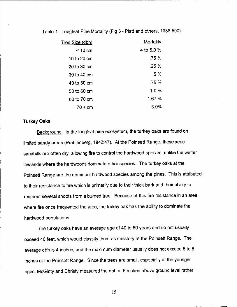
Mortality. Mortality in the longleaf pine is caused primarily by fire, beetles, wind,
disease, and old age, with fire the major cause of mortality (Conner and others,
1991:533). Some authors state that southern pine beetle infestation is not a normal
problem in longleaf pines, but cavity trees have less resistance and may actually attract
beetles (Conner and Rudolph, 1995:82,88-89). In cavity trees, mortality also increases
due to a higher susceptibility to fire and wind (Conner and others, 1991:532-533). A
typical intrinsic mortality rate for the longleaf pine is shown in Table 1. Fire plays an
integral part in tree health; once a tree is damaged by fire or lightning, bark beetle
infestation and disease often follow (Conner and others, 1991:532).
14
Mortality
4 to 5.0 %
.75 %
.25 %
.5%
.75 %
1.0%
1.67%
3.0%
Table 1. Longleaf Pine Mortality (Fig 5 - Platt and others, 1988:500)
Tree Size (dbh)
< 10 cm
10 to 20 cm
20 to 30 cm
30 to 40 cm
40 to 50 cm
50 to 60 cm
60 to 70 cm
70 +cm
Turkey Oaks
Background. In the longleaf pine ecosystem, the turkey oaks are found on
limited sandy areas (Wahlenberg, 1942:47). At the Poinsett Range, these xeric
sandhills are often dry, allowing fire to control the hardwood species, unlike the wetter
lowlands where the hardwoods dominate other species. The turkey oaks at the
Poinsett Range are the dominant hardwood species among the pines. This is attributed
to their resistance to fire which is primarily due to their thick bark and their ability to
resprout several shoots from a burned tree. Because of this fire resistance in an area
where fire once frequented the area, the turkey oak has the ability to dominate the
hardwood populations.
The turkey oaks have an average age of 40 to 50 years and do not usually
exceed 40 feet, which would classify them as midstory at the Poinsett Range. The
average dbh is 4 inches, and the maximum diameter usually does not exceed 5 to 6
inches at the Poinsett Range. Since the trees are small, especially at the younger
ages, McGinty and Christy measured the dbh at 6 inches above ground level rather
15
than the actual breast height (McGinty and Christy, 1976:488). When counting trees, a
group of sprouts from one root system counts as one tree, with the age and size of the
largest sprout being recorded, even though the root system may be much older.
According to McGinty and Christy, a successful species will produce more young than is
necessary to survive to maturity. When the young outnumber the old, the age structure
is stable (McGinty and Christy, 1976:489). The turkey oak achieves this stability by
sending several sprouts up from one root system even though only one tree per root
system is recorded.
Fire Effects. According to Rebertus the adult turkey oaks will tolerate mild
surface fires while the smaller turkey oaks are more prone to crown fires (Rebertus and
others, 1989:66). Although the crown fires kill the smaller trees, the trees will resprout,
usually within six months. The fire resistance increases as the trees become larger due
to the thicker bark and the higher crown height (Rebertus and others, 1989:66) Since a
slower crown death has a tendency to hinder resprout rates, a mild fire may be more
effective in controlling the turkey oak populations. Rebertus suggests that the highest
probability of killing the trees is found with a dbh between 3.1 and 4.3 inches, while
smaller trees have a high resprout rate and larger trees have a high survivability rate
(Rebertus and others, 1989:66).
Timber Value. The turkey oak is considered a forest weed along with other such
"scrub oaks" (Wahlenberg, 1942:248). The turkey oak has limited value as timber other
than the possible exception of firewood. At the Poinsett Range, this is not a viable
option due to the strafing mission and the need to protect the RCW habitat. Firewood
sales are currently limited to areas along main roads, which limits the economic
16
potential of this practice. The immediate requirement at Poinsett is to remove all
hardwood and pine saplings from within 50 feet of active clusters, leaving a basal area
of less than 10 feet squared per acre and no hardwoods greater than 1 inch dbh (Shaw
AFB, 1995:4). The long-term goal is to reduce the presence of the turkey oak from the
entire foraging area of the range through prescribed burning (Shaw AFB, 1995:9).
Removal currently consists of employees and volunteers physically cutting the trees,
because only hand clearing is permitted within the 200 foot buffer area of the cavities.
Even so, prescribed burning will be the method used for the rest of the range unless
burning is not feasible or is insufficient to control well advanced hardwood (Shaw AFB,
1995:5). Other options include mechanical removal via rotating blades, hydro axes,
and drum choppers. Another solution is the use of herbicides, but this practice is
limited by cost, herbicide control, and the undesired affect of killing flora other than the
turkey oak. Injecting the herbicide directly into the stump limits these problems while
keeping the turkey oak stump from resprouting. However the cost is still a factor and
this method is currently not used.
Effect on Wildlife. The turkey oak does have value as the primary source of
acorn production, which supports the various fauna at Poinsett. For instance, flying
squirrels were found to primarily feed on oak acorns; on average, 74.4% of their annual
diet is from oak acorns (Harlow, 1990:189). Their secondary source of food is from
pines; on average, 7.68% of their annual diet is from pine seeds and pollen (Harlow,
1990:189). However, the difference in food source is usually attributed to seasonal
variations, with acorn consumption occurring in the late fall and winter months and pine •
seed consumption occurring in the spring and summer months. Reducing the presence
17
of turkey oaks will have a significantly negative impact on the flying squirrels, which is
the primary competitor of the RCW for cavities. A reduction in food source will reduce
the squirrel population, while a reduction in midstory will reduce their protection and
increase predation. To maintain a healthy ecosystem with species other than the RCW,
some turkey oaks must remain to provide food and shelter to these species which
include deer, turkeys, fox squirrels, and flying squirrels.
Red-Cockaded Woodpecker
Background. The RCW is a federally listed endangered species (since 1970)
endemic to the southeastern United States. The RCW was once an abundant resident
of the southeastern Piedmont and Coastal Plain, ranging from New Jersey to Texas,
and inland to Kentucky, Tennessee, and Missouri (Jackson, 1971:4-29). Most
remaining populations are isolated, small, and fragmented, and continue to decline;
some populations are stable in their numbers, but none are increasing (Walters,
1991:507).
The RCW inhabits pine habitats, preferring mature longleaf pine savannahs
(U.S. Fish and Wildlife Service, 1985:1-88). It is nonmigratory and disperses short
distances for a bird its size (Walters and others, 1988:275-305). It is a cooperative
breeder, and thus its demography is characterized by the presence of nonbreeding
adults, usually males, long generation times and relatively low variance in reproductive
output among breeders (Ligon, 1970:255-278; Lennartz and others, 1987:77-88;
Walters and others, 1988:275-305; Walters, 1991)
Foraging Habitat. RCWs are nonmigratory and territorial throughout the year with
territories ranging from 125 to 370 acres in size (DeLotelle and Epting, 1987:258-294;
18
Hooper and others, 1982:675-682; Porter and Labisky, 1986:239-247; U.S. Fish and
Wildlife Service, 1985:1-88; Walters, 1991). The RCW primarily forages on live
longleaf pines for arthropods; reports of foraging time spent by RCWs on pines varies
from 90 to 95% (Lennartz and Henry, 1985:11; Hooper, 1996:115). The food source of
RCWs is made up of different arthropods; almost all of which are found on or in the
bark of longleaf pines (Hanula and Franzreb, 1995:488). This includes wood roaches
(69.4%), wood borer beetle larvae (5.4%), moth larvae (4.5%), spiders (3.6%), and ant
larvae and adults (3.1%).
The RCW obtains its food primarily by scaling bark and pecking. Although both
sexes forage on the upper trunk, only females regularly forage low on the trunk, and
only males forage regularly on the twigs and limbs (Walters, 1991:507). RCWs prefer
pines larger than 5 cm or 2 inches dbh, particularly those greater than 25 cm or 9.8
inches dbh for foraging (Hooper, 1996:115). Foraging area is directly related to pine
density (>/= 10 inches dbh) and inversely to hardwoods (>/= 5 inches dbh) (Lennartz
and Henry, 1985:11).
Over 60 ranges in the south have been studied for foraging area in relation to
RCWs and longleaf pine habitat. On average, 125 acres of pine habitat greater than 30
years in age is required for RCW foraging with approximately 24 pines per acre greater
than or equal to 10 inches dbh and less than 43 square feet basal area of hardwood
(Lennartz and Henry, 1985:12-16; Hooper, 1996:116). Approximately 40% of the
habitat in these studies was greater than 60 years of age and 94% of the foraging area
was within .5 miles of the clusters. According to the Shaw AFB RCW Management
Plan for Poinsett Weapons Range, their prime foraging habitat is established at 24
19
pines per acre greater than or equal to 10 inches dbh and 125 acres within .5 miles of
the active clusters (Shaw AFB, 1995:5). A population density goal set for RCWs is one
clan per 200 to 400 acres of pine and pine-hardwood forest (Lennartz and Henry,
1985:41).
Nesting Habitat. The RCW, unlike other woodpeckers, creates cavity nests in
living trees. It prefers longleaf pine forests, usually creating cavities in longleaf pine
trees 62 to 156 years of age, 20 to 30 feet above the ground (Ware and others,
1996:477; Conner and others, 1994:728). An average age for cavity trees noted by
several authors is 95 years, with age variation from 63 to 176 years (Lennartz and
Henry, 1985:5-6; Roise and others, 1990:7). Other authors have noted that as the
longleaf pine stand ages, the RCWs continually prefer the older trees (Rudolph and
Conner, 1991:459,461-462). The birds usually can only excavate cavities in the older
trees, because the cavity chamber must be excavated in the tree's heartwood core and
cannot extend into the surrounding sapwood (Walters, 1991:507).
RCW clusters are generally found in trees with densities of 10 to 150 square feet
basal area per acre (Lennartz and Henry, 1985:7). Hardwood is usually below 35
square feet basal area per acre and makes up less than 35% of the total stand with
average hardwood stocking at 20 square feet basal area per acre and 14% of total tree
density (Lennartz and Henry, 1985:8). By law, the cluster pine basal area is required to
be 14 to 16 square meters per hectare or 60.9 to 69.6 square feet basal area per acre
(Conner and Rudolph, 1995:82).
In a typical cluster, RCWs may form 1 to 30 cavities, depending on the RCW
cluster population (Lennartz and Henry, 1985:7). These cavities include actively
20
inhabited cavities, cavities being excavated or enlarged, and inactive or abandoned
cavities. Currently, the average number of cavities per cluster for the Poinsett Range
RCW population is 5.437 (Rogers, 1997). Trees within a cluster are usually inside a
1500 foot circle, but may be up to 2400 feet apart (Lennartz and Henry, 1985:7). The
Shaw AFB RCW Management Plan for Poinsett Weapons Range calls for all pine and
hardwood to be removed within 50 feet of all cavity trees (Shaw AFB, 1995:8).
Population Dynamics. RCWs are communal birds, with a breeding male and
female usually assisted by several helper birds. There are now six active clusters at the
Poinsett Range but only three breeding pairs with one helper per breeding pair (Rogers,
1997). There is no evidence that helpers participate in clutch production (Walters,
1990:508), but they assist in incubation and feeding of nestlings and fledglings
(Lennartz and others, 1987; Ligon, 1970:255-278). Many fledglings, nearly all females
and many males, disperse from their natal group during their first year to search for a
breeding vacancy (Walters, 1991:508). Although many early dispersers are breeders at
age one, some are individuals without a territory or mate, and some males are solitary,
having a territory but no mate (Walters, 1990:69-101). Three solitary males exist at the
Poinsett Range (Rogers, 1997). Individuals that remain on the natal territory and act as
helpers usually become breeders by inheriting breeding status through replacement of
a deceased individual (Walters, 1991:509).
RCWs compete for breeding vacancies in existing active clusters rather than
form new groups. This tactic is adopted by many males, but rarely by females (Walters,
1991:509). Thus, most helpers are natal males that delay dispersal and reproduction.
Once males acquire a breeding position they almost always hold it until they die, but
21
breeding females sometimes switch groups (Walters, 1990:69-101; Walters and others,
1988:275-305).
New groups, if formed, are created by occupying abandoned territories or
generating new territories. New territories are forged through pioneering in which a new
cluster of cavities is constructed in an unoccupied territory or budding in which an
existing territory and set of clusters is divided in two separate territories. Reoccupation
of abandoned territories seems to be the preferred method for forming new groups with
very little actual pioneering or budding observed in general, possibly due to the four to
seven year construction time for a cavity. (Walters and others, 1988:301; Walters,
1991:509; Barlow, 1995:729). For example, in a population of over 200 groups in the
Sandhills of North Carolina, only six new groups were formed from budding in eight
years, and pioneering was not observed (Copeyon and others, 1991:549). If a territory
is abandoned for more than two years, it usually remains abandoned (Walters,
1991:509).
Reproduction and Mortality. A group of RCWs produces a single nest within
each active cluster. The clutch size is two to four, averaging just over three throughout
the species' range (Ligon, 1970:255-278; Lennaratz and others, 1987:77-88).
Presently, the fertility rate for breeding pairs in the Poinsett Range territory is one
successful nest per year (Rogers, 1997). For particularly small isolated populations of
RCW such as the Poinsett Range, inbreeding may affect the overall fertility of the
population. Females rarely remain on their natal territories, and, if they do, avoid
related males (Walters, 1990:82).
22
Although the lifespan of an RCW can reach thirteen years, the typical lifespan of
an RCW for the Poinsett Range territory is four to five years (Barlow, 1995:729;
Rogers, 1997). Increased mortality of the RCW species is linked more to habitat loss
and alteration (loss of cavities) than to increased natural mortality or predation rates
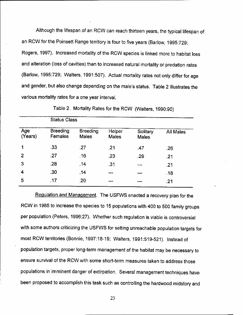
(Barlow, 1995:729; Walters, 1991:507). Actual mortality rates not only differ for age
and gender, but also change depending on the male's status. Table 2 illustrates the
various mortality rates for a one year interval.
Table 2. Mortality Rates for the RCW (Walters, 1990:90)
Status Class
Age Breeding (Years) Females
Breeding Males
Helper Males
Solitary Males
All Males
1 .33 .27 .21 .47 .26
2 .27 .16 .23 .29 .21
3 .28 .14 .31 — .21
4 .30 .14 — — .18
5 .17 .20 — — .21
Regulation and Management. The USFWS enacted a reco very plan for the
RCW in 1985 to increase the species to 15 populations with 400 to 500 family groups
per population (Peters, 1996:27). Whether such regulation is viable is controversial
with some authors criticizing the USFWS for setting unreachable population targets for
most RCW territories (Bonnie, 1997:18-19; Walters, 1991:519-521). Instead of
population targets, proper long-term management of the habitat may be necessary to
ensure survival of the RCW with some short-term measures taken to address those
populations in imminent danger of extirpation. Several management techniques have
been proposed to accomplish this task such as controlling the hardwood midstory and
23
understory, thinning pines within RCW cluster areas, utilizing cavity restrictors and
artificial cavities, translocating RCW breeders, and reintroducing breeding pairs to
abandoned territories (Conner and others, 1995:140). Artificial management
techniques such as cavity restrictors are relatively short-term measures while habitat
management plans such as controlling hardwood through prescribed burning can be
done to secure the long-term success of the RCW (Conner and others, 1995:149).
Cavity Competitors
Research suggests that the cavity nesting density of RCWs is not limited by the
number of cavities, but is a function of the total number of cavities in a given area and
the percentage of those cavities that are occupied by RCWs. This same research also
suggests that cavity competitors prefer RCW cavities over excavating new cavities in
snags, and that the main factor affecting occupation of RCW cavities by these cavity
competitor species is the abundance of the other species. (Everhart and others,
1993:41-42). Flying squirrels inhabit the same ecosystem as RCWs and are a major
competitor for RCW cavities (Harlow, 1990:187). The primary competitor for RCW
cavities observed by the Shaw Air Force personnel at the Poinsett Range is the
southern flying squirrel.
Flying Squirrel Cavity Preferences. One study concluded the flying squirrel
prefers enlarged RCW chambers, but does not show a preference for enlarged cavity
openings versus normal cavity openings (Rossell and Gorsira, 1996:23) However,
other studies have shown that the southern flying squirrel prefer cavities with smaller
entrances, entrance indices (vertical entrance diameter multiplied by horizontal
entrance diameter) of less than 50, and that flying squirrels prefer normal sized cavities
24
over enlarged cavities (Loeb, 1993:331-332). It should be noted in addition to using the
measurements at the entrance at the face of the tree, the Loeb study also used the
smallest vertical and horizontal diameters in the entry way and only examined cavities
for competitor habitation once per year (Loeb, 1993:330). A third study seems to verify
the flying squirrels preference for cavity openings with < 3.5 inches and points out that
flying squirrels can occupy cavities regardless of the quantity of the resin barrier
diameters (Rudolph and others, 1990:30,32).
Flying Squirrel Homes. The home-range for flying squirrels, considering the
horizontal landscape (planimetric area) has been observed at 9.4 acres and 19.3 acres
for female and male flying squirrels respectively (Stone and others, 1997:106). The
Stone study also observed that 54% of the flying squirrel den sites were in nest boxes,
and the remaining den sites were in natural cavities contained in snag or living trees.
(Stone and others, 1997:110-111). The squirrels typically use three or more different
cavities for their primary nest, escape nest and feed station (Sawyer and Rose,
1985:241). The flying squirrel will nest in nesting boxes, so the use of nesting boxes
increases the number of available primary nesting sites (Sawyer and Rose, 1985:242).
Flying squirrels have been found living in trees up to 46 feet away from the next nearest
tree which would suggest clearing the midstory away from cavity trees will not
effectively keep flying squirrels from RCW cavities (Loeb, 1993:333). Southern flying
squirrels are also able to return to their home range even when displaced up to 3280
feet (Sawyer and Rose, 1985:242)
Flying Squirrel Birth/Death Rates. Although exact birth and mortality rates could
not be found, it has be noted that the southern flying squirrel in North Carolina have 2.8
25
pups in their spring litter. While autumn litters for flying squirrels raised in captivity
averaged 4.0 pups per litter, but this may be inflated due to the effects of laboratory
rearing (Sawyer and Rose, 1985:242). Since the flying squirrel is a nocturnal animal,
owls are the major predator of the flying squirrel. For example, in Western North
America, flying squirrels make up at least half of the spotted owl's diet and a pair of
owls could consume 500 squirrels per year (Wells-Gosling, 1985:60). Although
predation of squirrels by snakes occurs in the southern states (Wells-Gosling, 1985:62),
experiments with the black rat snake have shown a low success rate (3 successful
climbs per 18 attempts) in climbing trees protected by a resin barrier (Rudolph and
others, 1990:19).
Flying Squirrel Foraging Habits. Studies of the food habits of the southern flying
squirrels from the coastal plain of South Carolina determined acorns are the major food
source for the squirrel year-round with the flying squirrels primarily feeding on oak
acorns; on average, 74.4% of their annual diet is from oak acorns (Harlow, 1990:189 -
190). Under ideal conditions it is estimated a squirrel could store 15,000 acorns in one
season (Wells-Gosling, 1985:80). Their second primary source of food is from pines; on
average, 7.68% of their annual diet is from pine seeds and pollen (Harlow, 1990:189).
Cavity Trees
RCW Cavity Tree Selection. Cavity tree selection by RCWs appears to be a
function of tree age as well as spatial characteristics. Studies indicate that RCWs
prefer longleaf pines that are an average age of 95 years for cavity initiation (Jackson
and others, 1979:102). However, many studies have found RCWs living in younger
trees due to the lack of older pines in an area and in these cases, the RCWs prefer
26
younger trees that have heartwood decay (Hooper, 1988:392-397). Conner found that
they also prefer younger trees with thinner sapwood and greater heartwood diameter
than other trees in the area. The RCW requires approximately 6 inches in diameter of
heartwood to excavate a cavity (Conner and others, 1994:732).
Spatial and forest characteristics also influence where RCWs prefer to roost.
The RCWs prefer cavity trees that are surrounded by fewer and shorter hardwoods.
Although studies have been performed on this behavior, researchers are unsure how
the midstory encroachment causes RCW population decline and if hardwood removal
will necessarily cause a return of the RCW (Kelly and others, 1993:126-127). Ross
found that the RCWs also prefer trees on the edge of tree stands because they are
healthier and have higher resin flows than trees on the interior of the stand. Generally,
open stands (stands with more edge trees) are kept open by frequent fires which create
a mosaic of clearings and healthier pines (Ross and others, 1997:151-152). Spatial
characteristics between RCW clusters are also important as noted by Thomlinson
(1996:352) who found that RCW clusters that became inactive were isolated from other
clusters or their tree stand became too small.
Cavity Tree Mortality. Cavity trees experience a higher mortality rate than typical
older pine trees and the major causes of mortality include bark beetles, wind snap, and
fire. In eastern Texas, bark beetles accounted for 53% of cavity tree mortality, wind
snap 30%, and fire 7%. However, the majority of these cavity trees were loblolly pine.
Of the 27 longleaf pine cavity tree deaths in the study, 33% were killed by prescribed
fire, 22% by bark beetles, 19% windsnapped, and 15% by old age. Longleaf pine cavity
trees are more vulnerable to fire due to the large amount of resin that seeps from resin
27
wells and flows close to the ground (Conner and others, 1991:534-536). This copious
production of resin also keeps longleaf pines from being as susceptible to southern pine
beetle infestation as compared to other southern pine species (Conner and Rudolph,
1995:82).
Cavity Enlargement. Cavity enlargement by pileated woodpeckers accounts for
another major loss of tree cavities. Conner and Rudolph's study in eastern Texas
found that 20% of known RCW cavities were enlarged over a seven year period
(Conner and others, 1991:535).
Cavity Creation and Protection. Artificial cavity creation and metal restrictor plate
installation are the primary management practices for increasing acceptable cavity
numbers. Artificial cavities are created through drilling or by installing a cavity insert,
which is basically a nesting box installed within the tree (Copeyon and others,
1991:550; Edwards and others 1997:231). The RCWs tend to prefer artificial cavities to
existing vacant natural cavities and the creation of artificial cavities has been successful
in increasing reoccupancy of abandoned clusters (Copeyon and others, 1991:554).
Metal restrictor plates are typically installed to restore enlarged cavity entrance holes
(greater than two inch diameter) or where the threat of enlargement is great (Shaw
AFB, 1995:5).
28

HI. Methodology
To successively meet the objectives of any environmental management
challenge, a specific plan or approach is necessary to ensure the field customer's
needs are satisfied in a timely manner. Deciding which approach is appropriate
depends on the nature of the problem and the client's objectives in solving the problem.
This particular consulting problem concerning the plight of the RCW and its habitat
centers on an ecosystem where change naturally occurs over time and the complexity
of such change stems from the internal interactions of the system as well as forces
external to the system. To understand the implications of various management
alternatives on such dynamic interrelationships, systems thinking and ecosystem
dynamics modeling prove ideal.
Typically, decisions which involve environmental issues consist of a large
number of influences that must be considered because environmental systems are
large and complex. People are unable to analyze several variables at a time which
often limits the complexity of their decision making (Gordon, 1885:4). Mental maps
(causal connections of the influences) seldom incorporate feedback loops, multiple
interactions, time delays, and non-linear interactions. Adding dynamic changes over
time introduces greater complexity which causes people to perform below potential
(Sterman, 1996:103-106). The system dynamics process accounts for feedback loops,
multiple interactions, time delays, non-linearity, and changes in the system over time.
The structure of the system dynamics process identifies the underlying mechanisms
that drive the basic system behavior. Policy maker's knowledge and system
29

information can be coded into the system dynamics model which enable the client to
understand both the short-term and long-term consequences of their management
alternatives (Morecroft, 1996:191).
For this project, the system dynamics approach allows for the exploration of
management alternatives which accomplish the clients overall objectives of maintaining
appropriate endangered species population levels and pursuing long-term stability for
the Poinsett Range ecosystem without sacrificing Air Force mission capability.
Accordingly, the methodology for this capstone project parallels the system dynamics
modeling process. It should be noted that the system dynamics process is an iterative
one, requiring the team to repeat and modify any one of the modeling stages as
necessary to ensure the model becomes a true mechanistic representation of the
ecosystem.
Conceptualization
To properly identify the problem to be solved, the team must become familiar
with the general problem scenario. The team must also continually interact with the
client to ensure the appropriate problem is addressed and to account for all client
concerns. (Three face-to-face meetings are planned along with both telephone and e-
mail contact as necessary.) It is during this process that the client may identify new
research questions, different approaches, various management practices, or even
discover that a system dynamics approach may not be appropriate for the questions
addressed.
Literature Review. Initially, an extensive literature review will be conducted in
order for the team to fully comprehend the entities and relationships driving ecosystem
30

behavior. The primary focus will be to determine what affects the behavior and habitat
of the chosen indicator species, the RCW. The literature review includes contacting the
client when necessary to answer specific Poinsett Range ecosystem questions and
consulting with available experts well-acquainted with the RCW and its habitat. It is
important that the literature review continue throughout the model building phase as
questions dealing with plausible parameter values, system mechanisms, and system
relationships arise. Once a general literature review is completed, a formal problem
statement will be derived.
Problem Statement. To delineate the client's objectives and define the question
to be addressed, an initial problem and purpose statement must be formulated. The
initial problem statement emphasizes the proper scope through which to solve the
problem. The purpose statement emphasizes the employment of the system dynamics
approach as the appropriate method in addressing the problem and accomplishing
client objectives. The client and project team will finalize the initial statements and
establish a joint consensus with regard to the appropriateness and scope of the
statements. Such consultation precludes any misunderstandings stemming from the
verbiage used to formulate the statements or the employment of the system dynamics
approach. Finally, minimum requirements for meeting objectives and system indicators
used to measure validity of the model will be jointly determined with the client. The
finalized problem and purpose statements are used to focus the overall modeling effort.
Reference Mode. A reference mode, or the expected behavior over the time
period of interest, is derived by analyzing the problem statement, available historical
31

data of the ecosystem, systems found in the literature, and client input. This reference
mode will be finalized by the project team after iterative review with the client.
Influence Diagram. An influence diagram representing cause-and-effect
relationships between the important entities which best represent the system will be
constructed by the project team. Using data gathered from the literature review, entities
essential to the ecosystem will be initially identified. Based upon this data and the
reference mode, the influences between these entities will be defined and should
generate feedback loops describing the basic mechanisms responsible for behavior of
the system. The level of aggregation and system boundary necessary to incorporate all
relevant entities and influences are determined by the questions the client wants the
project team to answer. Prior to coding the influence diagram into STELLA, a software
modeling package from High Performance Systems, the diagram will be presented to
the client to ensure that the diagram incorporates the basic mechanisms responsible for
ecosystem behavior and mechanistically describes the system's relationships. Due to
relevant client input and additional literature review, the influence diagram may be
altered accordingly to achieve the most accurate causal diagram.
Formulation
Model Construction. Once the system's mechanisms have been defined, flow
diagrams will be created to represent the mechanisms. The system dynamics model is
constructed by coding the flow diagrams into the STELLA computer modeling software
which utilizes the Euler method of numerical integration. The model will contain three
main sectors: RCW, cavities, and trees. Each sector postulates a detailed structure
depicting the flow diagrams with appropriate levels and rates selected from gathered
32

data. Equations defining such levels and rates, as well as any parameter values, will be
formulated from data and client input. Assumptions regarding any model formulations,
parameter values, or relationships will be documented and approved by the client
before being employed in the model.
Testing
Testing the Dynamic Hypothesis. Initial model runs will be conducted to
determine whether the basic mechanisms of the model reflect the reference mode. If
the model does not reflect the reference mode, additional review will be required to
determine if it includes all of the essential variables and mechanisms responsible for
system behavior, if the assumed relationships are reasonable, and if the parameter
values are plausible. Other validity tests which will be employed include: the extreme
conditions test which considers plausible maximum and minimum parameter values and
their effects on model output; the boundary adequacy test which analyzes behavior with
and without model structure; and the behavior anomaly test which traces anomalous
behavior back to a structural cause, leading to the identification of unrecognized
behavior in the real system.
Sensitivity testing, which identifies the attributes of the model most sensitive to
perturbations or manipulations of the model, will be conducted and reviewed with the
client. All model results will be compared to client intuition concerning the system.
Counterintuitive output will be examined to determine if modification of the model is
necessary. After testing is concluded, the model will be modified accordingly,
consulting with the client and performing additional literature review to correct any
33
discrepancies. Model structures will be modified until the project team and client are
satisfied the model is an accurate representation of the ecosystem under study.
Implementation
Testing Management Decisions/Policies. Specific predetermined management
scenarios, as requested by the client, will be applied to the model to test responses to
these policies. From the model runs, alternative strategies in managing the Poinsett
Range ecosystem will be explored to view the possible short- and long-range
consequences of the strategies.
Presentation of Findinas. Results from model runs will be consolidated and
translated into a useable form for the client to facilitate use of the model output for
decision-making purposes. Any counterintuitive results will be presented and explained
to ensure the client fully understands all of the phenomena driving ecosystem behavior.
Assumptions for the model, although previously discussed with the client, will be
reemphasized to ensure the context of the model's scope and structure is well
understood. The focus of the presentation will center on offering the client insight into
managing their ecosystem effectively while addressing the dilemmas associated with
balancing the concerns of the RCW, long-range Poinsett Range ecosystem stability,
and Air Force mission capability.
34
IV. Model Presentation
The system dynamics model structure for the project incorporates three major
sectors to represent the Longieaf Pine (LLP) ecosystem: tree, cavity, and Red-
Cockaded Woodpecker (RCW) sectors. The tree section, LLP and turkey oaks, is
based primarily on age class division and includes tree germination, tree health, tree
mortality, and tree mechanical removal. The cavity section focuses on total cavities in
the ecosystem and their construction by addressing acceptable and available cavities,
RCW occupied cavities, flying squirrel occupied cavities, unacceptable cavities, and
both artificial and natural cavity construction. The RCW section utilizes the RCW life
span as the basic building block for its structure. From the life span structure, critical
entities influencing the RCW population are modeled such as breeding pairs, cluster
availability, cavity availability, available helpers, foraging area, and inbreeding aversion.
Each sector of the model is structured according to numerous general and detailed
assumptions for the entities and their interrelationships. Appendix A lists the general
and detailed assumptions made for each sub-model.
Tree Sector Model Structure
The LLP population is divided into four age classes: 1 to 30 years, 30 to 60
years, 60 to 95 years, and 95 years and older. The maturation rate for these age
classes is assumed to be one divided by the number of years in age class. For
example, in the 1 to 30 year age group, 1/30 of the trees will mature and move to the
next higher age class each year. LLP populations are increased only by germination
from pine cones. An artificial planting rate can be assumed to be included in this
germination rate. The turkey oak population is handled as one age category, i.e. it is
not broken into various age classes.
Lonqleaf Pines (1 to 30 Years). The LLP from 1 to 30 years old have a dbh of
0 to 8 inches with an average dbh of 4 inches. LLPs from 1 to 30 years old have a
mortality rate, a mechanical removal rate (thinning/harvesting), and a maturation rate to
older pines. The mortality rate consists of natural mortality, percentage of deaths to
trees due to burning, Ips beetle infestation, and southern pine beetle infestation. The
ideal LLP under 30 years population is assumed to be 150 trees per acre over 8000
acres, or 1,200,000 trees total.
Lonqleaf Pines (30 to 60 Years). The LLP from 30 to 60 years old have a dbh of
8 to 16 inches with an average dbh of 12 inches. The trees in this age group are of
acceptable size to provide for good foraging area, but cavity construction is not yet
possible in these trees. LLPs from 30 to 60 years old have a mortality rate, a
mechanical removal rate (thinning/harvesting), and a maturation rate to older pines.
The mortality rate consists of natural mortality, percentage of deaths to trees due to
burning, Ips beetle infestation, and southern pine beetle infestation. The ideal LLP
density for the 30 to 60 years population is assumed to be 20 trees per acre over 8000
acres, or 160,000 trees total.
Lonqleaf Pines (60 to 95 Years). The LLPs from 60 to 95 years old have a dbh
of 16 to 20 inches with an average dbh of 18 inches. These trees are also acceptable
for foraging. Artificial cavities can be constructed in these trees. LLPs from 60 to 95
years old have a mortality rate, a mechanical removal rate (thinning/harvesting), and a
maturation rate to older pines. The mortality rate consists of natural mortality,
36
percentage of deaths to trees due to burning, Ips Beetle infestation, and southern pine
beetle infestation. The ideal LLP density for the 60 to 95 years population is assumed
to be 15 trees per acre over 8000 acres, or 120,000 trees total.
Longleaf Pines (95+ YearsV The LLPs over 95 years have a dbh over 20 inches
with an average dbh of 22 inches. These trees are also acceptable for foraging and
artificial cavity construction. LLPs in this age group are acceptable for natural cavity
construction by the RCWs. LLPs over 95 years are only removed from the system by
their mortality rate and a mechanical removal rate (thinning/harvesting). The mortality
rate consists of natural mortality, percentage of deaths to trees due to burning, Ips
Beetle infestation, and southern pine beetle infestation. The ideal LLP density for the
over 95 years population is assumed to be 10 trees per acre over 8000 acres, or
80,000 trees total.
Turkey Oaks. The turkey oak stock includes turkey oaks of all ages, with an
average dbh of 4 inches. Turkey oaks have a germination rate, a mortality rate, and a
mechanical removal rate. The mortality rate consists of natural mortality and
percentage of deaths to trees due to burning. The ideal turkey oak population is
assumed to be 50 trees per acre over 8000 acres, or 400,000 trees total.
Tree Germination. Shading by living trees is assumed to affect the successful
germination of both LLPs and turkey oaks. This is a factor that varies form 0 to 1 based
upon the density of turkey oaks and of LLPs, with turkey oaks having the greater impact
on shading (maximum value of 0.7), while the LLPs have less of an impact (maximum
value of 0.3). LLP shading is a function of LLP density and is represented graphically in
37

the mode!. Turkey oak shading is a function of turkey oak density and is also
represented graphically in the model.
Lonqleaf Pines. The LLP germination rate is a function of the total
number of LLPs and the total shading, which is determined by the total number of trees
per acre. Germination rates are higher when more sun is available as indicated
graphically in the model.
Turkey Oaks. Turkey oak germination is a function of the total number of
live turkey oaks and the total shading, which is determined by the total number of trees
per acre. Germination rates of turkey oaks are assumed to be not as drastically
affected by shading as are LLPs, as indicated by the graphical representation in the
model. It is assumed that 67% of the turkey oaks that die as a result of burning will re-
sprout.
Tree Health. Tree health for each group of LLPs varies with the burn health, the
mechanical removal health, and the basal area health for each group of LLPs, weighted
0.1, 0.3, and 0.6, respectively. The burn health for each tree group is a function of the
burn time, which increases from 0 to 1 as the years between burns (burn time) increase
from zero to a maximum of ten years (this reflects the fact that burning has some
negative impact on tree health). The burn time is set at a constant value of four years,
but can be altered to explore different management practices. The values are similar
for each group of trees. The mechanical removal health is a function of the removal
rate per area for each group of trees, which is discussed in the mechanical removal
section, and is represented graphically in the model for each LLP tree group. The basal
area health for each age group decreases as the total basal area per acre increases for
38
each LLP tree group, as represented graphically in the model (this recognizes the fact
that the health of individual trees is negatively impacted as total tree density increases,
due to root competition for nutrients and water).
Tree Mortality.
Natural mortality. For the LLPs, natural mortality for each tree group
varies inversely with total tree health for each tree group, as represented graphically in
the model.
Percentage of Deaths to Trees due to Burning The percentage of trees
in each age group that die directly from burning is a function of the fire intensity, as
represented by graphs in the model, with the LLPs resisting fire more as their age
increases. More turkey oaks burn as the fire intensity increases. All graphical
representations came from Shaw AFB personnel.
Fire Intensity. The fire intensity is a function of the level of fuel and the
stem density fire factor, each weighted equally. If there has been fire management in
the past, then the intensity will never exceed 0.75, otherwise it can vary from 1 (plentiful
fuel and a thick forest), to 0 (no fuel and an ideal density.)
Stem Density Fire Factor. The stem density fire factor is a function of the
stems density fire factors of the four LLP groups multiplied by their respective burn
weights, which are 0.5 for the 1 to 30 group, 0.3 for the 30 to 60 group, and 0.2 for 60 to
95 group and the 95+ group combined. As represented graphically, each tree group
stem density fire factor increases as the tree group stem density per acre increases.
FueL The level of fuel includes the fuel from both turkey oaks and LLPs
(multiplied by the time between burns), weighted 0.33 and 0.66, respectively. An
39

increase in the entity "bum time" reflects an increase in the time between burns. LLP
fuel level increases as the LLP basal area increases, as represented graphically in the
model, where basal area is the stem count per acre times the average radius squared
times %. Turkey oak fuel level also increases as the turkey oak basal area increases,
as represented graphically in the model, where again basal area is the stem count per
acre times the average radius squared times n.
Ips Beetle Infestation in Lonqleaf Pines. Ips beetle infestation decreases
as the total tree health for each group of LLPs increases, as represented graphically in
the model. When the total health varies from 0.2 to 1, the Ips beetle infestation factor
varies from 0.02 to 0.002. Beetle infestation rates are approximately the same for each
tree age category.
Southern Pine Beetle Infestation in Lonqleaf Pines. The southern pine
beetle infestation decreases as the total health for each group of LLPs and is indicated
graphically. When total health is 0, the infestation rate is 0.905. The rate drops off
until it reaches 0 when total health equals 0.4. The rate remains at 0 while the total
health varies from 0.4 to 1. Beetle infestation rates are the same for each tree age
category.
Tree Mechanical Removal. The mechanical removal rate for LLP represents
thinning for pulpwood, while for the turkey oaks it represents clearing all hardwoods in
the area. It is assumed the trees with weaker health will be removed, and any removal
will increase the health of the entire stand. The removal rate is the excess trees divided
by the time between thinning, which is set at eight years for the LLPs and four years for
the turkey oaks. The excess trees are the difference between the ideal stem density
40

and the actual stem density. Note that if the ideal is greater than the actual, then no
mechanical removal will occur.
Cavity Sector Model Structure
The basic structure of the cavity sub-model is a set of four stocks representing all
cavity trees. These stocks are acceptable and available cavities, RCW occupied
cavities, flying squirrel occupied cavities, and unacceptable cavities due to enlargement
by pileated woodpeckers. The combined total of each of these stocks yields the total
number of cavities which is initially 87, based on information from Shaw AFB. The total
number of cavities can be reduced only through cavity tree mortality.
The loss of cavity trees is based upon the increased mortality of LLPs due to the
weakening of the infrastructure as a result of cavities. The literature indicates that the
cavity tree mortality rate is 0.013 deaths/tree/year (Conner and others, 1991:534-536).
This cavity tree loss is inclusive for all four stocks of cavities and is slightly higher than
the mortality rates of LLPs without cavities. The cavity tree mortality rate cannot be
used as a constant but instead must represent the increased mortality of cavity trees
versus normal LLPs. The LLP mortality rate is essentially the literature based mortality
rates of two stocks of cavity-free trees weighted by their population to provide a
representative mortality rate of all the mature trees in the model. After determining the
mortality rate of LLPs over 60 years old as a result of natural and human generated
events in the tree sub-model, we augment this with an increased mortality rate
representing increased cavity tree susceptibility. The mortality rate of both LLPs and
cavity trees can be found in the literature. The difference gives us a "delta" which can
augment the LLP mortality determined in the tree sub-model. As a result, this cavity
41
tree mortality rate should mimic the ill effects placed upon the trees in the tree sub-
model due to beetle infestation, fire, wind snap, and so forth, but with slightly increased
mortality due to increased cavity tree susceptibility.
Acceptable and Available Cavities. Initially there are 54 acceptable available
cavities. More cavities are created at a construction rate based on pioneering and
artificial cavity construction. Artificial cavity construction accounts for up to 20 cavities
per year if the number of available cavities is low. Pioneering accounts for up to 3
cavities per year if the number of available cavities is low. Both rates decrease if the
tree density falls below the optimum of 60 to 80 square feet per acre. The construction
rate is never allowed to exceed the number of LLPs available, whether it is LLPs 60
years and older for artificial cavity construction or LLPs 95 years and older for natural
cavity construction. Available cavities are lost to cavity tree mortality, RCW or squirrel
occupancy, and to enlargement.
RCW Occupied Cavities. Twelve cavities are initially occupied by RCWs based
on figures from Shaw AFB. Cavity occupancy increases and decreases as the adult
RCW population changes each year. Fledglings are not considered to occupy their own
cavity since they share a cavity with a parent. Thus, only one through six year old birds
can change the number of RCW cavities occupied. However, overall cavity occupancy
is not solely based on RCWs but also includes competitor occupancy.
Flying Squirrel Occupied Cavities. Initially, 20 cavities are occupied by flying
squirrels, based on data from Shaw AFB. Squirrel occupancy changes based on the
change in overall squirrel population multiplied by the fraction of squirrels which occupy
RCW cavities less the amount of squirrel boxes installed.
42

Competitor Population Growth. The inflow for the competitor stock is controlled
by the competition birth rate (the number of squirrels born per year) and is the product
of the number of competitors times the birth rate of two pups per squirrel. The birth rate
was calculated per squirrel by taking the literature value of five pups per year, dividing
by two to account for the number of squirrels per breeding pair, and then multiplying by
the fraction of squirrels of breeding age (4/5 or 80%). Since the squirrels are not
assumed to be controlled by top down predation, the availability of food is believed to
affect squirrel birth rates. Therefore, a food factor is used as a multiplier for the overall
birth rate. The food factor is represented graphically in the model and ranges from zero
(where the food per squirrel value is zero) to one (where the food per squirrel value is
20). The turkey oak basal area divided by the competitor stock is used to represent the
availability of food per squirrel.
Competitor Population Decline. The outflow of the competitors stock is a sum of
the number of squirrels captured per year plus the number of competitors lost each
year due to predation and mortality. The predation and mortality rates are multiplied by
the number of competitors in the stock. The mortality rate is set at 0.5 and is multiplied
by the mortality switch (1=on; 0=off), which allows the mortality rate to be turned either
on or off. The predation rate is represented graphically and ranges from one, when
there are no turkey oaks to provide cover from predation, to near 0.01, when there are
enough turkey oaks to provide cover from predation. The capture rate is also
represented graphically, and ranges from 0, when there are only 20 cavities occupied
by squirrels, to 100, when there are 100 cavities occupied by squirrels.
43
Competition Pressure. The competition pressure (in squirrels/year) is the net
number of increase in squirrels per year that would be looking to occupy a cavity. It is
calculated by taking the difference between the squirrel birth rate and the loss rate and
then multiplying this difference by the fraction of squirrels that choose to live in cavities
versus building their own den. Finally, the squirrels that occupy the squirrel boxes are
subtracted to provide the final value for competition pressure.
Unacceptable Cavities. There are initially 20 unacceptable cavities due to
enlargement by pileated woodpeckers. This stock is influenced by the rate of metal
restrictor plates installed and the rate of enlargement by pileated woodpeckers. Once a
restrictor plate is installed, the cavity is considered available and acceptable again. The
enlargement rate begins at 0.0318 enlargements/tree/year (Conner and others,
1991:535). This rate decreases as the rate of restrictor plate installation increases.
This is based on the assumption that cavities with restrictor plates cannot be enlarged.
Red-Cockaded Woodpecker (RCW) Sector Model Structure
The RCW sub-model attempts to model the significant entities and relationships
influencing the RCW population while utilizing a basic life span structure for the RCW.
The sub-model focuses on the influences which affect the birth, death, and departure
rates of the RCW population. The RCW population is also dynamically affected by the
adequacy of its foraging area and the number of available cavities per cluster. In many
cases, the foraging area and the number of available cavities will be the limiting factor
for the RCW population. The limitations to the RCW population presented by foraging
area and available cavities is defined in the tree and cavity sub-models. The number of
breeding pairs, the foraging area, and the number of helpers per breeding pair are the
44
factors assumed to be most influential in the population's birth rate based on the
literature review. The death rate is assumed to be driven primarily by natural mortality
and predation while the departure rate can fluctuate due to the absence of a mate, lack
of adequate clusters, lack of acceptable cavities, and lack of adequate foraging area.
RCW Key Entities and Relationships
Breeding pairs. Breeding pairs are a function of the number of males and
females and the availability of cavities per cluster. It is assumed only one breeding pair
will occupy a cluster. The sub-model determines the potential number of breeding pairs
by pairing each male RCW of breeding age to a female RCW of breeding age. It is
assumed that birds matched for breeding are unrelated. A breeding pair will stay in the
managed area only if there are two acceptable and available cavities in a cluster the
pair can occupy; otherwise, the female RCW will depart and the male RCW will remain
in the area to become a helper (if there are an adequate number of cavities). It is
apparent that the RCW population birth rate will increase with the number of breeding
pairs.
Helpers per breeding pair. It is assumed in this model that only males of
breeding age without a mate are eligible to become helpers. If a male RCW does not
have a mate, the male will become a helper only if an adequate cavity is available
within a cluster. Otherwise, the male RCWs is assumed to depart the managed area.
The fledgling mortality rate is assumed to equal the natural mortality rate
of fledglings when the breeding pair has no helpers. The fledgling mortality rate will
decrease as the number of helpers per breeding pair increases. The decrease in the
45
mortality rate will remain constant when each breeding pair has an average of four or
more helpers.
Foraging area. Foraging area is defined in this model as the basal area of
LLPs 30 years and older within the area of management concern. Each individual
RCW requires a certain basal area to provide its nutritional requirement of insects. The
quality of the foraging area is determined by comparing the required basal area per bird
with the actual basal area per bird. The foraging area is assumed to be adequate if the
actual basal area per bird equals or exceeds the minimally required basal area.
It is assumed that a minimum area of foraging area is required to produce
the "normal" amount of fledgling per breeding pair. If the available foraging area
exceeds this amount, the birth rate is not effected; if the foraging area is less than the
minimum required, the production rate of each breeding pair diminishes.
The foraging area will also influence the departure rate of the RCW from
an area of management concern. Poor foraging area will enhance the departure rate of
breeding age males and females from the area of management concern. Adequate
foraging area will not necessarily prevent birds from departing; RCWs will still depart
due to a lack of a mate or lack of an acceptable cavity.
Mortality Rate. The mortality rate applied to the RCW population includes
the effects of predation, disease, strafing deaths, and natural mortality. The mortality
rates for the male and female fledgling stock are decreased by the number of helpers
per breeding pair which is less than four.
Departure Rate. The total number of male and female RCWs departing
an area of management concern are represented by two separate entities. The number
46
of birds departing are divided equally over the respective stocks representing the male
and female RCWs of breeding age.
The female departure rate is determined by the availability of a mate and
the availability of adequate cavities. Additionally, the female departure rate can
increase due to inbreeding aversion represented by a relatedness factor which is
described in the RCW Model Limitation section. Male RCW departure is influenced
primarily by the availability of adequate cavities. Poor foraging area will accelerate both
the female and male departure rates.
RCW Model Limitations. Simplifying assumptions were required to model the
mechanisms driving the changes in an RCW population. These assumptions were
necessary in order to capture the essence of the complex social structure, breeding
activity, and foraging habits of the RCW. Many of the mechanisms associated with the
birds behavior such as the female RCWs instinct to depart rather than inbreed and the
RCWs decision to depart an area rather than stay and foray are not well understood.
However, entities representing these behavior patterns have been incorporated in the
model with simple mechanisms to ensure these important influences on the RCW
population are addressed accordingly. These limitations will also be discussed in the
"Model Strengths and Weaknesses" section of Chapter 5.
Incest Avoidance and Loss of Genetic Diversity. As stated previously, it is
assumed in the model that the number of new breeding pairs within an area of
management concern is dependent solely upon the availability of a mate and the cavity
availability for a breeding pair. The assumption that female RCWs will stay within a
managed area as long as they can find a mate is accurate as long as there is an
47
abundance of unrelated birds. Typically, female RCWs will depart its cluster to find an
unrelated male for a mate rather than inbreed. The incest avoidance instincts of the
female RCW makes inbreeding among RCW separated by a single generation rare.
However, inbreeding among distant relatives is not unlikely, particularly when the RCW
population is isolated. Inbreeding would attribute to a population's loss of genetic
diversity; consequently, the fertility rate of an RCW population may be adversely
affected if extensive inbreeding occurs.
Relatedness Index. The influence of the female RCWs instincts to avoid
inbreeding is represented by the entities "Relatedness" and "Relatedness Index". The
two entities define the general relationship expected between the RCW population size
and the tendency for a female RCW to depart an area due to its incest avoidance
instincts. It is assumed that as the RCW population decreases, the percentage of
genetically related male and female RCWs will increase. The percentage of genetically
related males and females will be minimized as the total RCW population exceed 25
birds. Consequently, the female RCW departure rate will increase as the RCW
population decreases over an extended period (when the total RCW population is less
than 25 birds).
Genetic Diversity Loss. In small and isolated RCW populations such as
Poinsett Range, the likelihood for inbreeding increases. Intuitively, extended periods of
inbreeding may diminish the fertility rate of breeding pairs, increase the mortality rate of
fledglings, and diminish the RCW population's ability to combat certain diseases. The
effects of extended interbreeding on the RCW population is not addressed in the
model.
48
Artificial Translocation. Artificial translocation is a management practice
which brings RCWs from areas outside a particular managed area into the managed
area. This management practice may be used to enhance the genetic pool of an RCW
population or to increase the number of breeding pairs in the area. At the Poinsett
Range, the RCW population is isolated, and the active clusters within the range consist
of birds that are related. This situation suggests that artificial translocation is necessary
in order to sustain the RCW population. Some efforts at artificial translocating birds into
the Poinsett Range have been made, although the success of this action has not yet
been determined.
The translocation of birds is represented in this model through an
additional inflow of birds into the stocks of females and males one through three years
of age. It is assumed in this model that only younger male and female RCWs of
breeding age would be transplanted into the area to maximize the available number of
breeding years and minimize mortality. In the baseline runs of the model, the artificial
translocation rate for both male and female birds are set to zero. Translocation of birds
out of the area is not considered in this model.
Foraging Area and the Effect on Immigration and Emigration. It is
assumed the RCW will depart the area of management concern at an accelerated rate
if the foraging area is below the minimum area necessary to meet each bird's nutritional
requirement of insects. The model assumes the managed area is contiguous to
suitable RCW habitat which can provide the necessary basal area, and the natural
immigration rate of birds into the managed area is negligible.
49
Overall Model Interaction
Although each sector represents a separate critical piece to the overall Poinsett
Range ecosystem, the junction points connecting each sector of the model prove critical
in establishing the overall behavior of the ecosystem. The tree sector determines how
many cavities can be constructed and how many cavities remain acceptable and
available for use. The cavity sector distributes the number of cavities appropriately
based on competitor and RCW levels while accounting for those cavities lost to cavity
tree mortality and unacceptable cavities. Moreover, the cavity sector ultimately
determines the allowable number of clusters available for the RCW. The RCW
population can fluctuate based on cavities and cluster numbers as well as foraging
area. These links between the sectors are crucial to the model's ability to
mechanistically represent the behavioral trends of the Poinsett Range ecosystem.
50
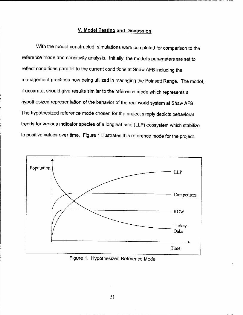
V. Model Testing and Discussion
With the model constructed, simulations were completed for comparison to the
reference mode and sensitivity analysis. Initially, the model's parameters are set to
reflect conditions parallel to the current conditions at Shaw AFB including the
management practices now being utilized in managing the Poinsett Range. The model,
if accurate, should give results similar to the reference mode which represents a
hypothesized representation of the behavior of the real world system at Shaw AFB.
The hypothesized reference mode chosen for the project simply depicts behavioral
trends for various indicator species of a longleaf pine (LLP) ecosystem which stabilize
to positive values over time. Figure 1 illustrates this reference mode for the project.
Figure 1. Hypothesized Reference Mode
51
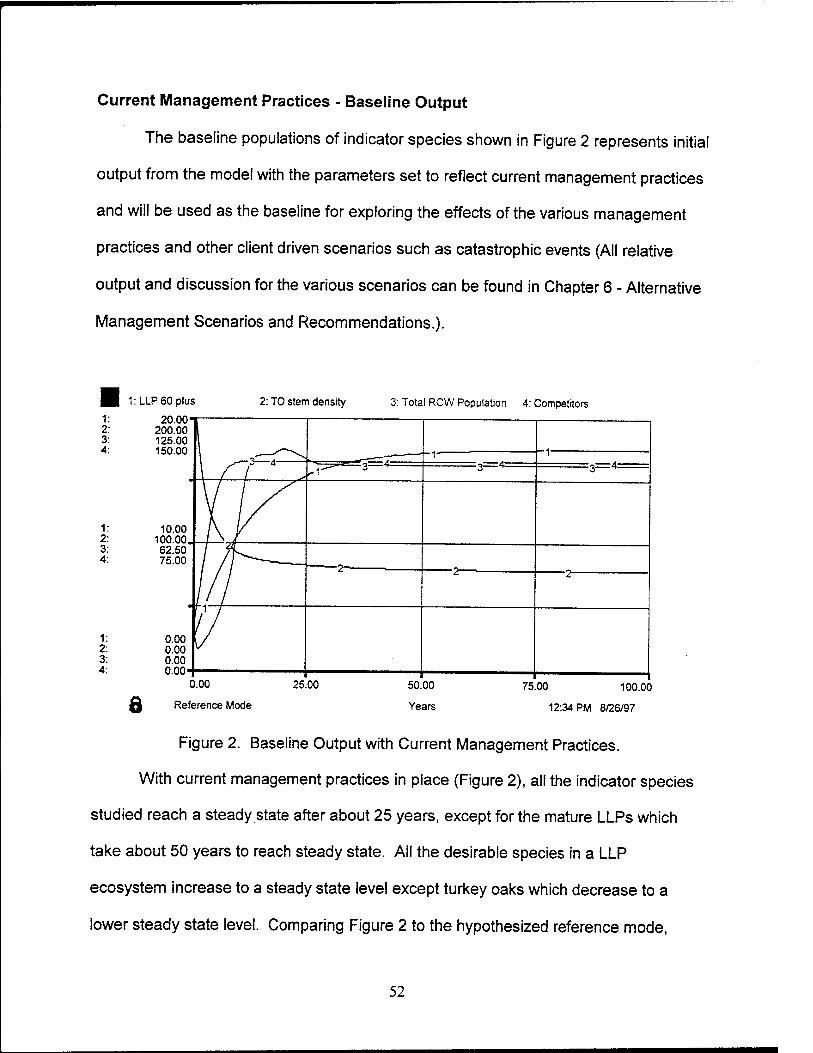
Current Management Practices - Baseline Output
The baseline populations of indicator species shown in Figure 2 represents initial
output from the model with the parameters set to reflect current management practices
and will be used as the baseline for exploring the effects of the various management
practices and other client driven scenarios such as catastrophic events (All relative
output and discussion for the various scenarios can be found in Chapter 6 - Alternative
Management Scenarios and Recommendations.).
1:LLP60plus
20.00 T 200.00 125.00 150.00
2: TO stem density 3: Total RCW Population 4: Competitors
10.00 100.00 62.50 75.00
0.00 0.00 0.00 0.00
6 0.00
Reference Mode
25.00 50.00
Years
75.00 100.00
12:34 PM 8/26/97
Figure 2. Baseline Output with Current Management Practices.
With current management practices in place (Figure 2), all the indicator species
studied reach a steady state after about 25 years, except for the mature LLPs which
take about 50 years to reach steady state. All the desirable species in a LLP
ecosystem increase to a steady state level except turkey oaks which decrease to a
lower steady state level. Comparing Figure 2 to the hypothesized reference mode,
52
Figure 1, one can conclude the basic mechanisms of the constructed model create the
reference mode; therefore, it appears the overall dynamic hypothesis of the Poinsett
Range system has been successfully modeled.
Validation Testing
Model testing must also incorporate testing model assumptions to ensure the
model includes the important variables, the assumed relationships are reasonable, and
the parameter values are plausible. Because system dynamics modeling concentrates
on overall system trends instead of predicting precise numbers, standard statistical
tests are not used to validate the systems dynamics model structure (Forrester,
1996:421). Confidence was gained in the model through iterative inspection and use
by the client and through the application of five validity tests: Structure Verification,
Parameter Verification, Extreme Conditions, Boundary Adequacy, and Behavior
Anomaly.
Structural Verification. First the structure and influences were developed from
and compared to the mechanisms discovered during the literature review. Further
structural verification was performed by comparing the actual structure of the model
with the structure of the real world system. Moreover, by explaining the detailed model
structure to the client, the team and client were able to ensure the model structure was
reasonable, there were no contradictions between the model and the real world system,
and the assumptions in the model were valid. The structure of the model was revised
through an iterative process based on discussions with the client during the three field
trips to Shaw AFB.
53

Parameter verification. Parameter verification was conducted conceptually by
reviewing the parameters with the user to ensure the parameters encoded in the model
actually existed and matched elements in the real system. The numerical values and
ranges of the parameters were reviewed with and verified by the client.
Extreme Conditions. The model's behavior under extreme conditions was tested
by setting the stocks and rates to realistic real world extreme conditions and observing
the behavior of the model. It was important that the model did not crash or that the
responding behavior seemed realistic and was explainable. The section "Sensitivity
Analysis" of this chapter presents a more detailed discussion of using extreme
conditions for model testing.
Structural Boundary Adequacy. Structure Boundary Adequacy was validated by
explaining to the client the aggregation of real world influences incorporated into the
system dynamics model. The client also reviewed the model to ensure all relevant
structure had been included and that no plausible hypothesis could be proposed that
indicated the need for additional mode entities or mechanisms. For example, the
suggestion that a beaver consumption mechanism be added would not be realistic,
since this is not a plausible entity for this system. Behavior Boundary Adequacy was
verified by ensuring the addition or removal of model structure did not affect the model's
behavior. More time should to be spent testing the mode! by adding additional
structure; however, an example of excessive structure in the model is the tree foraging
area mechanism. This mechanism was never activated by the model during testing
under extreme conditions, and could be removed without affecting the behavior of the
model.
54
Behavior Anomaly. Behavior anomalies, such as stocks or rates remaining
constant or changing erratically during the model simulation, were observed during the
initial coding and running of the model. This often indicated the model needed revision
so the model more accurately reflects the mechanisms of the real world system. The
model was also tested to see if it showed implausible behavior when the assumptions
were altered. Surprise behavior, when an unnoticed behavior of the real system
surfaces, was also discovered. For example, translocation of the RCWs does not
produce a higher population than natural population growth. This may seem
counterintuitive, until it was considered that the birds were introduced into the system
too quickly before acceptable cavities could be prepared for them. As a result, the
homeless translocated RCWs would leave the system.
Sensitivity Testing
By varying different parameters in the model through extreme values, an
indication of their significance to model output was established. This process of
sensitivity testing allows modelers to identify parameters which are the most sensitive
and others which are not. Sensitive variables can then be closely scrutinized to ensure
their input values are accurate.
55
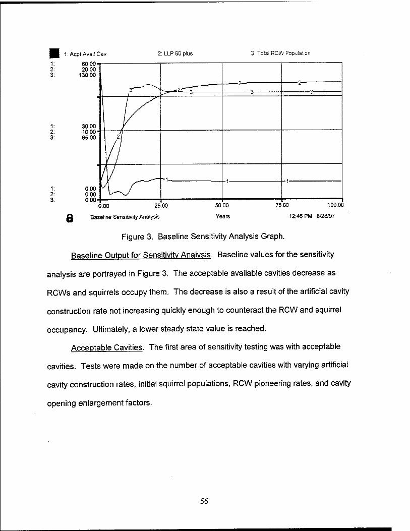
1: Acpt Avail Cav
60.00 20.00
130.00
2: LLP 60 plus 3 Total RCW Population
30.00 10.00 65.00
0.00 0.00 0.00
8 0.00 25.00
Baseline Sensitivity Analysis
50.00
Years
75.00 100.00
12:46 PM 8/28/97
Figure 3. Baseline Sensitivity Analysis Graph.
Baseline Output for Sensitivity Analysis. Baseline values for the sensitivity
analysis are portrayed in Figure 3. The acceptable available cavities decrease as
RCWs and squirrels occupy them. The decrease is also a result of the artificial cavity
construction rate not increasing quickly enough to counteract the RCW and squirrel
occupancy. Ultimately, a lower steady state value is reached.
Acceptable Cavities. The first area of sensitivity testing was with acceptable
cavities. Tests were made on the number of acceptable cavities with varying artificial
cavity construction rates, initial squirrel populations, RCW pioneering rates, and cavity
opening enlargement factors.
56
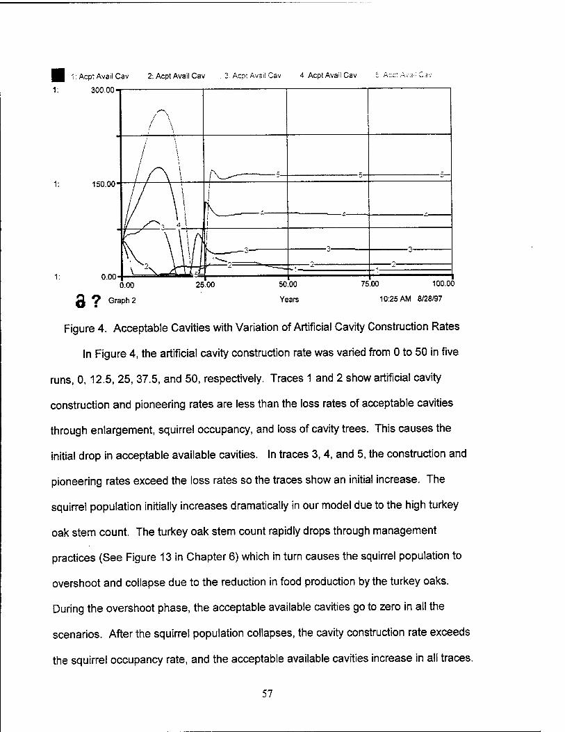
I 1: Acpt Avail Cav 2: Acpt Avail Cav 3. Acpt Avail Cav 4: Acpt Avail Cav
1: 300.00-
1: 150.00-
0.00 0.00
3 9 Graph 2
25.00 50.00
Years
75.00 100.00
10:25 AM 8/28/97
Figure 4. Acceptable Cavities with Variation of Artificial Cavity Construction Rates
In Figure 4, the artificial cavity construction rate was varied from 0 to 50 in five
runs, 0,12.5, 25, 37.5, and 50, respectively. Traces 1 and 2 show artificial cavity
construction and pioneering rates are less than the loss rates of acceptable cavities
through enlargement, squirrel occupancy, and loss of cavity trees. This causes the
initial drop in acceptable available cavities. In traces 3, 4, and 5, the construction and
pioneering rates exceed the loss rates so the traces show an initial increase. The
squirrel population initially increases dramatically in our model due to the high turkey
oak stem count. The turkey oak stem count rapidly drops through management
practices (See Figure 13 in Chapter 6) which in turn causes the squirrel population to
overshoot and collapse due to the reduction in food production by the turkey oaks.
During the overshoot phase, the acceptable available cavities go to zero in all the
scenarios. After the squirrel population collapses, the cavity construction rate exceeds
the squirrel occupancy rate, and the acceptable available cavities increase in all traces.
57
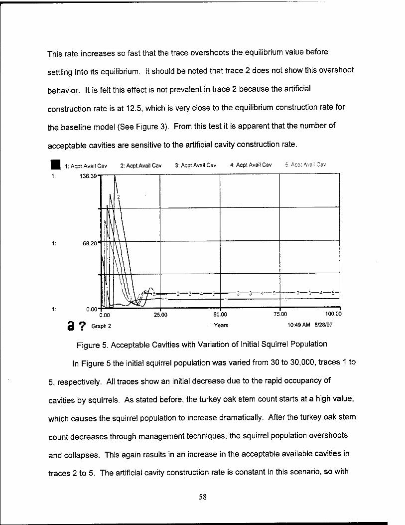
This rate increases so fast that the trace overshoots the equilibrium value before
settling into its equilibrium. It should be noted that trace 2 does not show this overshoot
behavior. It is felt this effect is not prevalent in trace 2 because the artificial
construction rate is at 12.5, which is very close to the equilibrium construction rate for
the baseline model (See Figure 3). From this test it is apparent that the number of
acceptable cavities are sensitive to the artificial cavity construction rate.
■I 1:Acpt Avail Cav 2: Acpt Avail Cav 3: Acpt Avail Cav 4: Acpt Avail Cav
1: 136.39'
3: Avail Cav
68.20
1: 0.00 0.00
3 1 Graph 2
25.00 —I 50.00
Years
—, 75.00 100.00
10:49 AM 8/28/97
Figure 5. Acceptable Cavities with Variation of Initial Squirrel Population
In Figure 5 the initial squirrel population was varied from 30 to 30,000, traces 1 to
5, respectively. All traces show an initial decrease due to the rapid occupancy of
cavities by squirrels. As stated before, the turkey oak stem count starts at a high value,
which causes the squirrel population to increase dramatically. After the turkey oak stem
count decreases through management techniques, the squirrel population overshoots
and collapses. This again results in an increase in the acceptable available cavities in
traces 2 to 5. The artificial cavity construction rate is constant in this scenario, so with
58
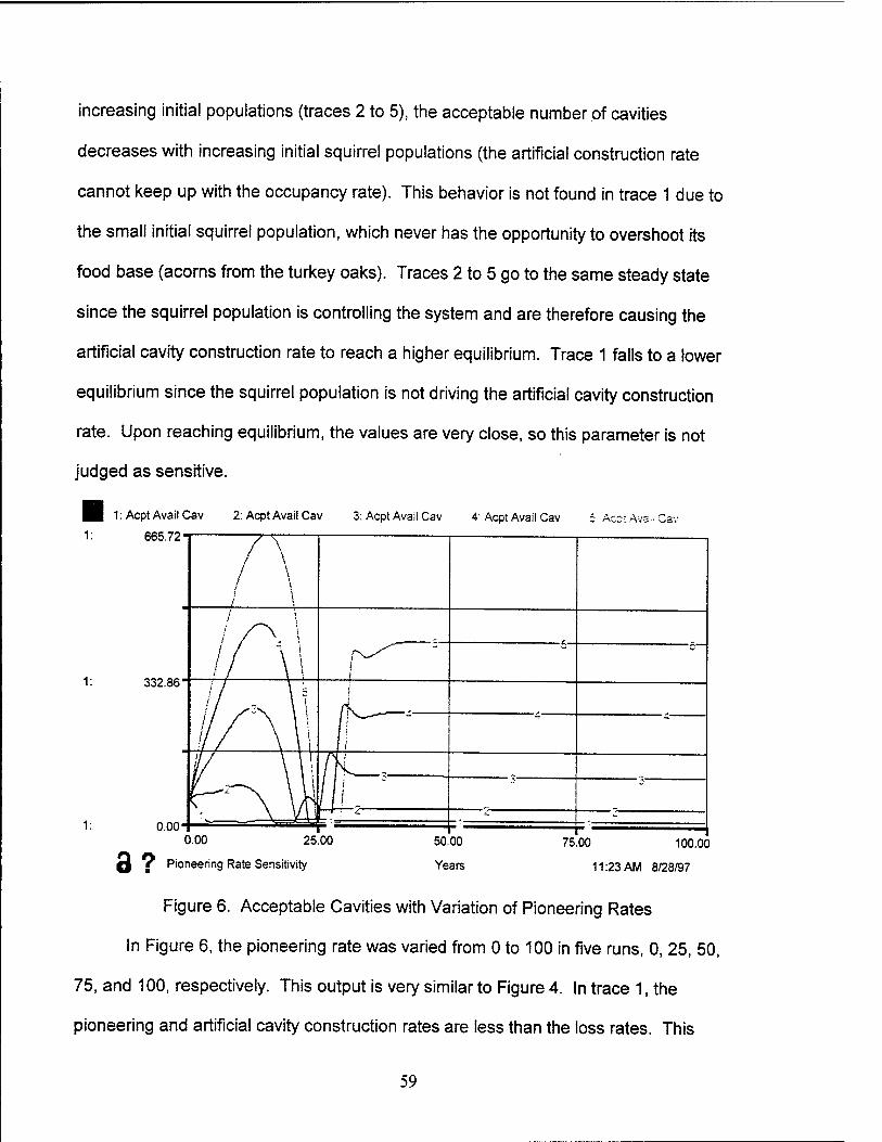
increasing initial populations (traces 2 to 5), the acceptable number of cavities
decreases with increasing initial squirrel populations (the artificial construction rate
cannot keep up with the occupancy rate). This behavior is not found in trace 1 due to
the small initial squirrel population, which never has the opportunity to overshoot its
food base (acorns from the turkey oaks). Traces 2 to 5 go to the same steady state
since the squirrel population is controlling the system and are therefore causing the
artificial cavity construction rate to reach a higher equilibrium. Trace 1 falls to a lower
equilibrium since the squirrel population is not driving the artificial cavity construction
rate. Upon reaching equilibrium, the values are very close, so this parameter is not
judged as sensitive.
1: 1: Acpt Avail Cav 2: Acpt Avail Cav 3: Acpt Avail Cav 4: Acpt Avail Cav 5 AcotAvs Cav
665.72 T
332.86
0.00 0.00 25.00
Q V Pioneering Rate Sensitivity
50.00
Years
75.00 100.00
11:23 AM 8/28/97
Figure 6. Acceptable Cavities with Variation of Pioneering Rates
In Figure 6, the pioneering rate was varied from 0 to 100 in five runs, 0, 25, 50,
75, and 100, respectively. This output is very similar to Figure 4. In trace 1, the
pioneering and artificial cavity construction rates are less than the loss rates. This
59
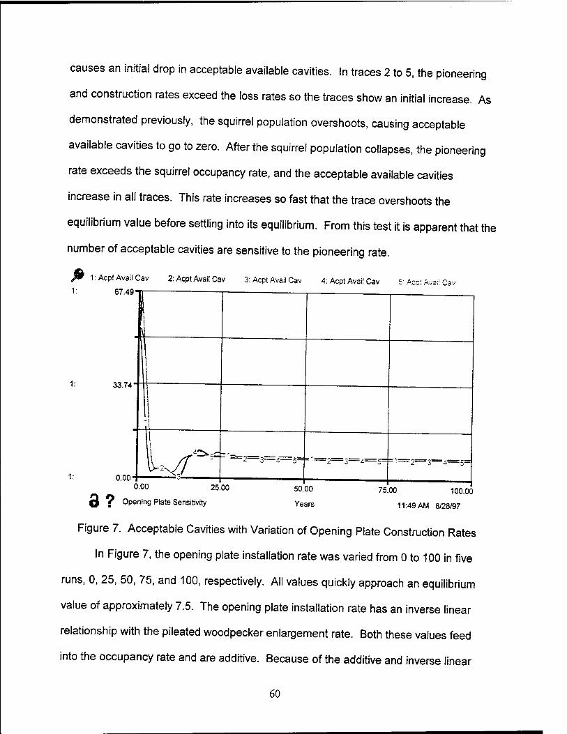
causes an initial drop in acceptable available cavities. In traces 2 to 5, the pioneering
and construction rates exceed the loss rates so the traces show an initial increase. As
demonstrated previously, the squirrel population overshoots, causing acceptable
available cavities to go to zero. After the squirrel population collapses, the pioneering
rate exceeds the squirrel occupancy rate, and the acceptable available cavities
increase in all traces. This rate increases so fast that the trace overshoots the
equilibrium value before settling into its equilibrium. From this test it is apparent that the
number of acceptable cavities are sensitive to the pioneering rate.
1: Acpt Avail Cav 2: Acpt Avail Cav 3: Acpt Avail Cav 4: Acpt Avail Cav 5: Ace: Avail Cav
1: 67.49 TT
33.74-
0.00 0.00 25.00
Q V Opening Plate Sensitivity
50.00
Years
75.00 100.00
11:49 AM 8/28/97
Figure 7. Acceptable Cavities with Variation of Opening Plate Construction Rates
In Figure 7, the opening plate installation rate was varied from 0 to 100 in five
runs, 0, 25, 50, 75, and 100, respectively. All values quickly approach an equilibrium
value of approximately 7.5. The opening plate installation rate has an inverse linear
relationship with the pileated woodpecker enlargement rate. Both these values feed
into the occupancy rate and are additive. Because of the additive and inverse linear
60
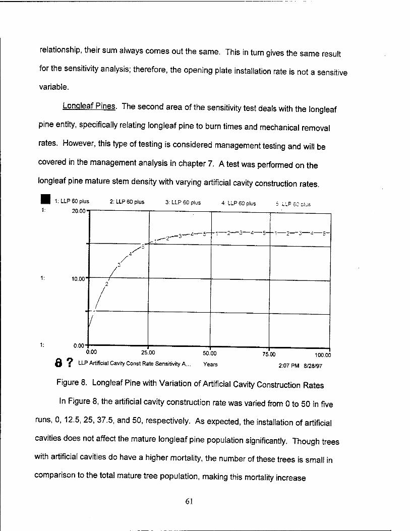
relationship, their sum always comes out the same. This in turn gives the same result
for the sensitivity analysis; therefore, the opening plate installation rate is not a sensitive
variable.
Longleaf Pines. The second area of the sensitivity test deals with the longleaf
pine entity, specifically relating longleaf pine to burn times and mechanical removal
rates. However, this type of testing is considered management testing and will be
covered in the management analysis in chapter 7. A test was performed on the
longleaf pine mature stem density with varying artificial cavity construction rates.
1:LLP60plus
20.00 T
2: LLP 60 plus 3: LLP 60 plus 4: LLP 60 plus LLF 60 clus
10.00-
/
/
/
o.oo ■+ 0.00 25.00 50.00
O f LLP Artificial Cavity Const Rate Sensitivity A... Years
—I— 75.00 100.00
2:07 PM 8/28/97
Figure 8. Longleaf Pine with Variation of Artificial Cavity Construction Rates
In Figure 8, the artificial cavity construction rate was varied from 0 to 50 in five
runs, 0, 12.5, 25, 37.5, and 50, respectively. As expected, the installation of artificial
cavities does not affect the mature longleaf pine population significantly. Though trees
with artificial cavities do have a higher mortality, the number of these trees is small in
comparison to the total mature tree population, making this mortality increase
61
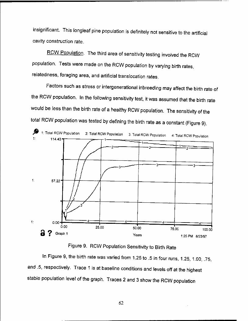
insignificant. This longleaf pine population is definitely not sensitive to the artificial
cavity construction rate.
RCW Population. The third area of sensitivity testing involved the RCW
population. Tests were made on the RCW population by varying birth rates,
relatedness, foraging area, and artificial translocation rates.
Factors such as stress or intergenerational inbreeding may affect the birth rate of
the RCW population. In the following sensitivity test, it was assumed that the birth rate
would be less than the birth rate of a healthy RCW population. The sensitivity of the
total RCW population was tested by defining the birth rate as a constant (Figure 9).
1: Total RCW Population 2: Total RCW Population 3: Total RCW Population 4: Total RCW Population 1: 114.43 T
57.22-
1: 0.00" 0.00
Q *? Graph 1
25.00 50.00
Years
75.00 100.00
1:25 PM 8/23/97
Figure 9. RCW Population Sensitivity to Birth Rate
In Figure 9, the birth rate was varied from 1.25 to .5 in four runs, 1.25, 1.00, .75,
and .5, respectively. Trace 1 is at baseline conditions and levels off at the highest
stable population level of the graph. Traces 2 and 3 show the RCW population
62
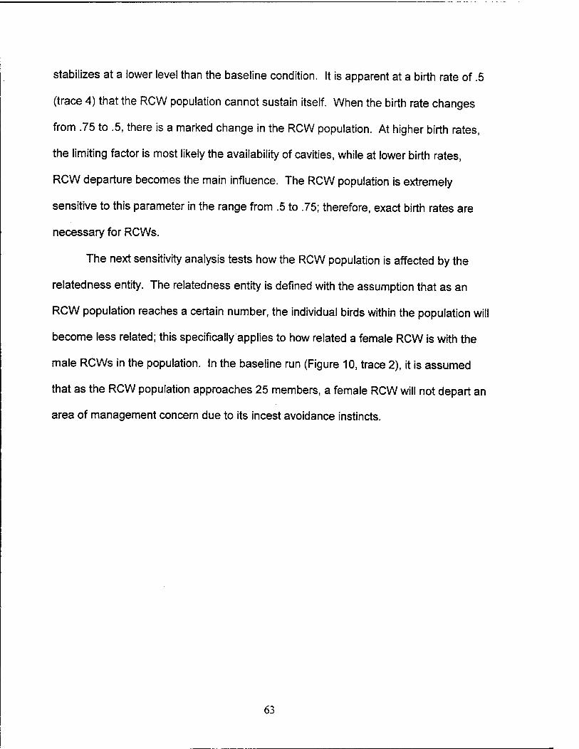
stabilizes at a lower level than the baseline condition. It is apparent at a birth rate of .5
(trace 4) that the RCW population cannot sustain itself. When the birth rate changes
from .75 to .5, there is a marked change in the RCW population. At higher birth rates,
the limiting factor is most likely the availability of cavities, while at lower birth rates,
RCW departure becomes the main influence. The RCW population is extremely
sensitive to this parameter in the range from .5 to .75; therefore, exact birth rates are
necessary for RCWs.
The next sensitivity analysis tests how the RCW population is affected by the
relatedness entity. The relatedness entity is defined with the assumption that as an
RCW population reaches a certain number, the individual birds within the population will
become less related; this specifically applies to how related a female RCW is with the
male RCWs in the population. In the baseline run (Figure 10, trace 2), it is assumed
that as the RCW population approaches 25 members, a female RCW will not depart an
area of management concern due to its incest avoidance instincts.
63
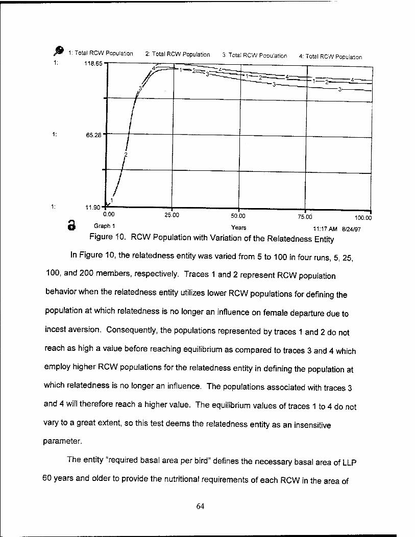
1: Total RCW Population 2: Total RCW Population 3: Total RCW Population 4: Total RCW Population
1: 118.65 T
65.28
1: 11.90-N" I 75.00 0.00 25.00 50.00
O Graph 1 Years 11:17 AM 8/24/97
Figure 10. RCW Population with Variation of the Relatedness Entity
In Figure 10, the relatedness entity was varied from 5 to 100 in four runs, 5, 25,
100, and 200 members, respectively. Traces 1 and 2 represent RCW population
behavior when the relatedness entity utilizes lower RCW populations for defining the
population at which relatedness is no longer an influence on female departure due to
incest aversion. Consequently, the populations represented by traces 1 and 2 do not
reach as high a value before reaching equilibrium as compared to traces 3 and 4 which
employ higher RCW populations for the relatedness entity in defining the population at
which relatedness is no longer an influence. The populations associated with traces 3
and 4 will therefore reach a higher value. The equilibrium values of traces 1 to 4 do not
vary to a great extent, so this test deems the relatedness entity as an insensitive
parameter.
The entity "required basal area per bird" defines the necessary basal area of LLP
60 years and older to provide the nutritional requirements of each RCW in the area of
——i 100.00
64
management concern. The foraging area quality is based on the value set in this entity.
The foraging area has a two-fold effect on the RCW population; the foraging area
quality will enhance the departure rate of mature male and female RCW and diminish
the fertility rate of each breeding pair that remains in the area (Figure 11).
1: Total RCW Population
1: 137.3&1 2: Total RCW Population 3: Total RCW Population
1: 71.33"
1: 5.31 0.00
Q ? Graph 20
•1 2—3-
25.00 50.00
Years
75.00 100.00
10:08 AM 8/28/97
Figure 11. RCW Population with Variation of Foraging Area per RCW
In Figure 11, the foraging area per RCW entity was varied from 1 to 600 in three
runs, 1, 60, and 600, respectively. Given that legislation only requires 125 basal area
for a cluster, these values cover the expected range of values for this parameter. All
three traces are exactly the same; they follow the baseline output. Therefore, RCW
population is not sensitive to this parameter.
65
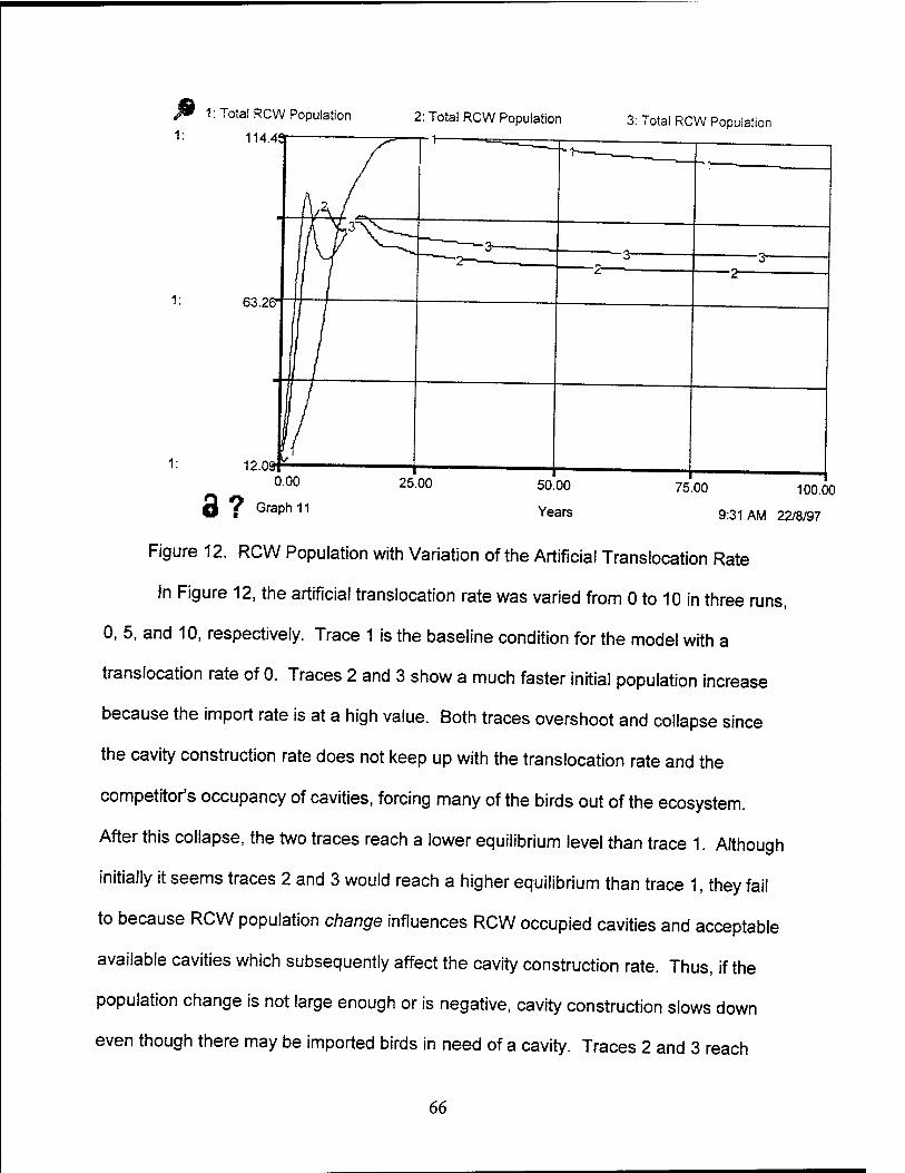
1: Total RCW Population
1: 114.4»
2: Total RCW Population 3: Total RCW Population
1: 63.20-"
12.09 0.00
3 ? Graph 11 25.00 50.00
Years
75.00 100.00
9:31 AM 22/8/97
Figure 12. RCW Population with Variation of the Artificial Translocation Rate
In Figure 12, the artificial translocation rate was varied from 0 to 10 in three runs,
0, 5, and 10, respectively. Trace 1 is the baseline condition for the model with a
translocation rate of 0. Traces 2 and 3 show a much faster initial population increase
because the import rate is at a high value. Both traces overshoot and collapse since
the cavity construction rate does not keep up with the translocation rate and the
competitor's occupancy of cavities, forcing many of the birds out of the ecosystem.
After this collapse, the two traces reach a lower equilibrium level than trace 1. Although
initially it seems traces 2 and 3 would reach a higher equilibrium than trace 1, they fail
to because RCW population change influences RCW occupied cavities and acceptable
available cavities which subsequently affect the cavity construction rate. Thus, if the
population change is not large enough or is negative, cavity construction slows down
even though there may be imported birds in need of a cavity. Traces 2 and 3 reach
66

steady state at lower population levels due to fewer cavities being constructed, a result
of the lack of a significant positive population change as seen in trace 1. This
sensitivity test shows the RCW population is sensitive to the translocation rate.
Model Strengths and Weaknesses
From the model's initial output, validation testing, and sensitivity analysis, the
model's strengths and weaknesses were discovered and then evaluated based on the
model's success in answering the research questions posed by the client by running
long-range simulations and in helping the client to understand the basic mechanisms
driving ecosystem behavior. Recall the research questions focus on the effects of
ecosystem management and RCW management practices on the viability of the LLP
ecosystem as defined by tree composition, density, and age structure.
Model Strenqths. The main strength of the model lies in the model structure
which allows for long-term simulations of a wide variety of scenarios important to the
interests of the client. These scenarios involve combinations of ecosystem
management practices, RCW management practices, and naturally occurring
environmental impacts. The output of the model simulations can be used by the client
to evaluate proposed management strategies and to prepare for the impacts of
naturally occurring events.
The model building process and model simulation output served as an effective
aid to the client in developing a deeper understanding of the influences which affect the
managed ecosystem and in tying together intuitions about the ecosystem's behavior
under various scenarios. The process of constructing the model required the client to
examine the entities within the ecosystem, to determine the relationships between each
67
entity, and to weigh and evaluate the influence of each relationship. This process
enabled the client to further develop his intuition and understanding with regards to the
interrelationships occurring within the managed ecosystem. Through the model
building process the client developed a firm understanding of the assumptions used in
the model and gained confidence that the model structure incorporated the entities and
relationships necessary to answer the research questions. As a result, the client was
well qualified to evaluate the validity of the model simulation output.
The model output effectively communicated to the client the potential
consequences resulting from various management and environmental scenarios. The
graphical output of these simulations served as a convenient way to evaluate the
system's behavior under varied conditions. The model output was validated against the
client's expectations of the system's behavior under the scenarios tested. Thus, the
model served as affirmation of the client's current expectations for the system's
behavior and as a basis for discussion in cases where the client's expectations of
system behavior were not met.
Model Weaknesses. The main weaknesses of the model stem primarily from the
inability of the model structure to capture the unique characteristics of the RCW habitat
and population at Poinsett Range. Other weaknesses in the model are linked to the
relationship between tree density and artificial cavity construction rate.
The basic model was constructed under the assumption that the ecosystem is a
homogenous forest area adjacent to other forest areas of similar characteristics. The
RCW habitat at Poinsett is actually small and fragmented with a patchwork of wetlands,
sandhills, plantation forest, and fire roads. Additionally, the range is relatively isolated
68
from other forest areas. Since the project assumed homogeneous and isolated
conditions for the range habitat and "averaged" cavities and clusters over the area, the
model fails to address the implications of forest fragmentation and edge effects on the
RCW population. Several authors feel that fluctuations in population can occur based
on the presence of forest fragmentation or location of clusters in an area on the edge of
the habitat (Rudolph and Conner, 1994:365-375; Walters, 1991), but the effects of
habitat fragmentation and isolation on the behavior of the RCW are not completely
understood. Further study in this area could alter the model given the current model's
assumptions which ignore fragmentation and edge effects altogether.
Due to the relatively isolated nature of the Poinsett Range habitat, it is possible
that female birds may choose to stay within the ecosystem rather than depart into
unsuitable habitat adjacent to the managed area. This isolation also prevents adequate
immigration of birds into the managed area. These two major influences may lead to
eventual inbreeding and may reduce breeding altogether.
Female RCWs have been known to avoid breeding with closely related males
(Walters, 1991). This phenomena can have an enormous impact on the RCW
population especially for an isolated habitat such as the Poinsett Range. The limited
number of birds reduces the number of unrelated males available for breeding, thereby,
severely reducing birth rates for a given population. Such a small population ultimately
leads to a reduction in the species gene pool with dubious consequences for the RCW
population in the area.
Currently, the effects of such inbreeding is represented by a "relatedness" factor
which suggest the female RCW will depart from the ecosystem based on the size of the
69
RCW population, regardless of how isolated the ecosystem may be from other suitable
ecosystems. The mechanisms involved in the female RCWs decision to depart an area
or to stay and risk the chances of inbreeding are not well understood. Although the
current model attempts to address genetic diversity and incest aversion with the simple
mechanism relating total population to relatedness, the model needs a more detailed
representation of genetic diversity and its effects in order to completely depict the
mechanism responsible for incest aversion.
The second major weakness of the model involves the rate at which cavities are
artificially constructed. Although tree density is currently employed in the model to
determine cavity goodness and, subsequently, cavity construction, it is based on overall
tree density. Cavity goodness does not account for the effects of varying the type of
tree controlling cavity goodness; therefore, turkey oak tree density can supplant
longleaf pine density and still create favorable conditions for cavity construction. There
should be some negative feedback based upon turkey oak density. As turkey oak
density increases, the cavity construction should decrease, since an area with heavy
turkey oak understory or midstory is unsuitable for cavities and cavities for the RCW are
built in longleaf pines only. However, the current model does ensure cavity construction
fluctuates with increasing or decreasing tree density itself. The model only fails to
address the different types of trees affecting tree density and the implications of varying
the mixture of tree density on cavity construction. The cavity construction rate would be
more accurately reflected if the rate is based solely on the density of LLP 60 years or
older.
70
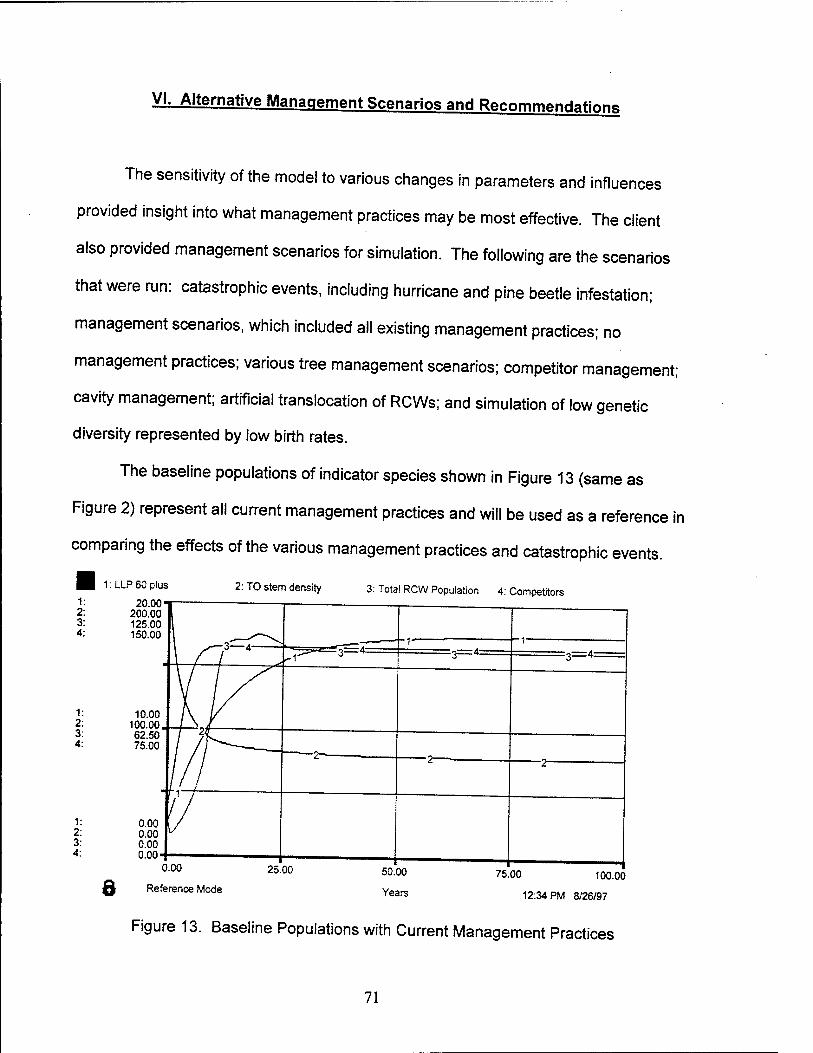
VI. Alternative Management Scenarios and Recommendation«
The sensitivity of the model to various changes in parameters and influences
provided insight into what management practices may be most effective. The client
also provided management scenarios for simulation. The following are the scenarios
that were run: catastrophic events, including hurricane and pine beetle infestation;
management scenarios, which included all existing management practices; no
management practices; various tree management scenarios; competitor management;
cavity management; artificial translocation of RCWs; and simulation of low genetic
diversity represented by low birth rates.
The baseline populations of indicator species shown in Figure 13 (same as
Figure 2) represent all current management practices and will be used as a reference in
comparing the effects of the various management practices and catastrophic events.
1: UP 60 plus
20.00-r-
200.00 125.00 150.00
2: TO stem density 3: Total RCW Population 4: Competitors
10.00 100.00 62.50 75.00
6 Reference Mode Years
75.00 100.00
12:34 PM 8/26/97
Figure 13. Baseline Populations with Current Management Practices
71
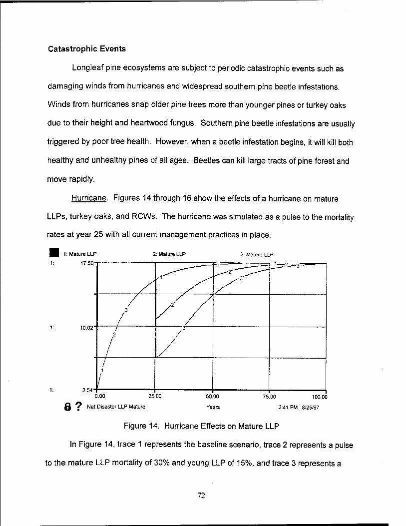
Catastrophic Events
Longleaf pine ecosystems are subject to periodic catastrophic events such as
damaging winds from hurricanes and widespread southern pine beetle infestations.
Winds from hurricanes snap older pine trees more than younger pines or turkey oaks
due to their height and heartwood fungus. Southern pine beetle infestations are usually
triggered by poor tree health. However, when a beetle infestation begins, it will kill both
healthy and unhealthy pines of all ages. Beetles can kill large tracts of pine forest and
move rapidly.
Hurricane. Figures 14 through 16 show the effects of a hurricane on mature
LLPs, turkey oaks, and RCWs. The hurricane was simulated as a pulse to the mortality
rates at year 25 with all current management practices in place.
■ 1: Mature LLP
1: 17.50-T
2: Mature LLP 3: Mature LLP
10.02
2.54 0.00 25.00
Q *? Nat Disaster LLP Mature
50.00
Years
75.00 100.00
3:41 PM 8/25/97
Figure 14. Hurricane Effects on Mature LLP
In Figure 14, trace 1 represents the baseline scenario, trace 2 represents a pulse
to the mature LLP mortality of 30% and young LLP of 15%, and trace 3 represents a
72
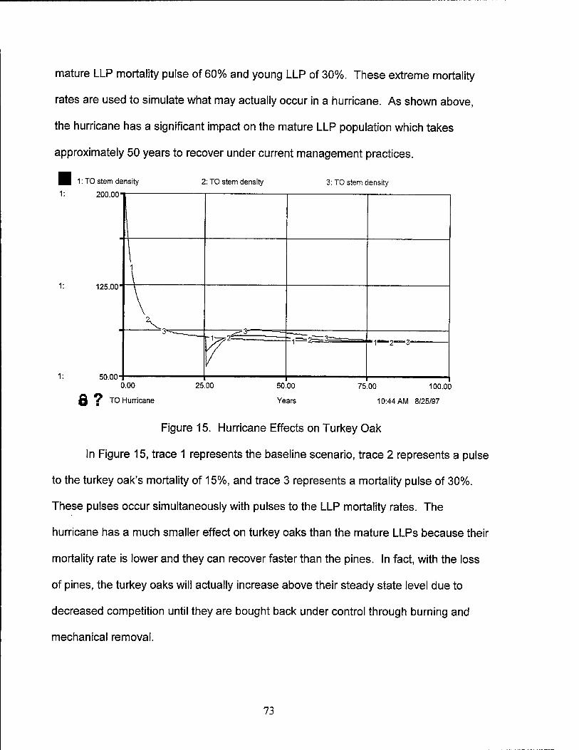
mature LLP mortality pulse of 60% and young LLP of 30%. These extreme mortality
rates are used to simulate what may actually occur in a hurricane. As shown above,
the hurricane has a significant impact on the mature LLP population which takes
approximately 50 years to recover under current management practices.
stem de nsity 2: TO stem density 3: TO stem density
«iUU.UU
I I
1
\ 125.00"
\
°' — ^-3 ' r-1~^52— 2= 1 <
,^—,
V ou.uun
0.00
Q 7 TO Hurricane
25.00 50.00
Years
75.00 100.00
10:44 AM 8/25/97
Figure 15. Hurricane Effects on Turkey Oak
In Figure 15, trace 1 represents the baseline scenario, trace 2 represents a pulse
to the turkey oak's mortality of 15%, and trace 3 represents a mortality pulse of 30%.
These pulses occur simultaneously with pulses to the LLP mortality rates. The
hurricane has a much smaller effect on turkey oaks than the mature LLPs because their
mortality rate is lower and they can recover faster than the pines. In fact, with the loss
of pines, the turkey oaks will actually increase above their steady state level due to
decreased competition until they are bought back under control through burning and
mechanical removal.
73
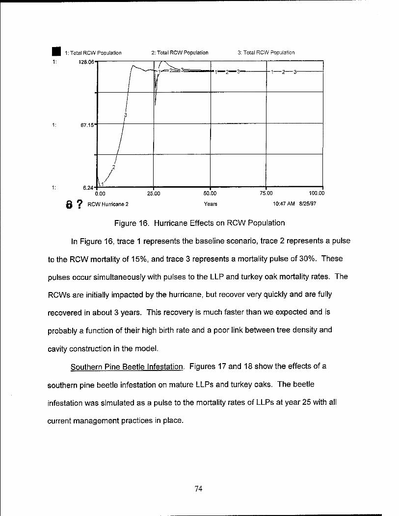
■ 1: Total RCW Population
1: 128.06
2: Total RCW Population 3: Total RCW Population
67.15-
6.24
/x_
f " I """"V 3 1 2 3
3 /
I
./ /
2
0.00
Q *? RCW Hurricane 2
25.00 50.00
Years
75.00 100.00
10:47 AM 8/25/97
Figure 16. Hurricane Effects on RCW Population
In Figure 16, trace 1 represents the baseline scenario, trace 2 represents a pulse
to the RCW mortality of 15%, and trace 3 represents a mortality pulse of 30%. These
pulses occur simultaneously with pulses to the LLP and turkey oak mortality rates. The
RCWs are initially impacted by the hurricane, but recover very quickly and are fully
recovered in about 3 years. This recovery is much faster than we expected and is
probably a function of their high birth rate and a poor link between tree density and
cavity construction in the model.
Southern Pine Beetle Infestation. Figures 17 and 18 show the effects of a
southern pine beetle infestation on mature LLPs and turkey oaks. The beetle
infestation was simulated as a pulse to the mortality rates of LLPs at year 25 with all
current management practices in place.
74
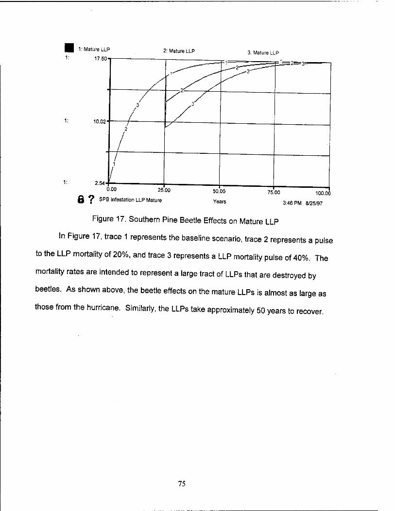
■ 1: Mature LLP 1: 17.50-r
2: Mature LLP 3: Mature LLP
10.02-
1: 2.54 0.00 25.00
Q *? SPB Infestation LLP Mature
50.00
Years
75.00 100.00
3:46 PM 8/25/97
Figure 17. Southern Pine Beetle Effects on Mature LLP
In Figure 17, trace 1 represents the baseline scenario, trace 2 represents a pulse
to the LLP mortality of 20%, and trace 3 represents a LLP mortality pulse of 40%. The
mortality rates are intended to represent a large tract of LLPs that are destroyed by
beetles. As shown above, the beetle effects on the mature LLPs is almost as large
those from the hurricane. Similarly, the LLPs take approximately 50 years to recover.
as
75
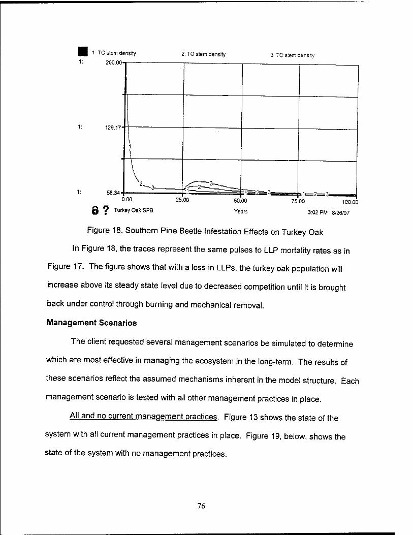
HI 1: TO stem density
1: 200.00T
2: TO stem density 3" TO stem density
129.17-
58.34 0.00
Q *? Turkey Oak SPB
25.00 50.00
Years
75.00 100.00
3:02 PM 8/26/97
Figure 18. Southern Pine Beetle Infestation Effects on Turkey Oak
In Figure 18, the traces represent the same pulses to LLP mortality rates as in
Figure 17. The figure shows that with a loss in LLPs, the turkey oak population will
increase above its steady state level due to decreased competition until it is brought
back under control through burning and mechanical removal.
Management Scenarios
The client requested several management scenarios be simulated to determine
which are most effective in managing the ecosystem in the long-term. The results of
these scenarios reflect the assumed mechanisms inherent in the model structure. Each
management scenario is tested with all other management practices in place.
All and no current management practices. Figure 13 shows the state of the
system with all current management practices in place. Figure 19, below, shows the
state of the system with no management practices.
76
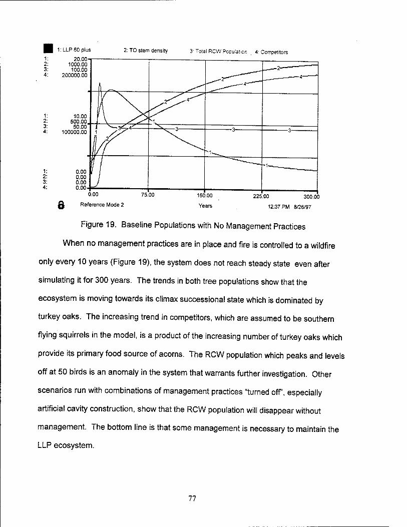
1: LLP 60 plus
20.001- 1000.00 100.00
200000.00
2: TO stem density 3'Total RCW Population 4: Competitors
10.00 500.00
50.00 100000.00
0.00 0.00 0.00 0.00
8 Reference Mode 2
150.00
Years
225.00 300.00
12:37 PM 8/26/97
Figure 19. Baseline Populations with No Management Practices
When no management practices are in place and fire is controlled to a wildfire
only every 10 years (Figure 19), the system does not reach steady state even after
simulating it for 300 years. The trends in both tree populations show that the
ecosystem is moving towards its climax successional state which is dominated by
turkey oaks. The increasing trend in competitors, which are assumed to be southern
flying squirrels in the model, is a product of the increasing number of turkey oaks which
provide its primary food source of acorns. The RCW population which peaks and levels
off at 50 birds is an anomaly in the system that warrants further investigation. Other
scenarios run with combinations of management practices "turned off', especially
artificial cavity construction, show that the RCW population will disappear without
management. The bottom line is that some management is necessary to maintain the
LLP ecosystem.
77
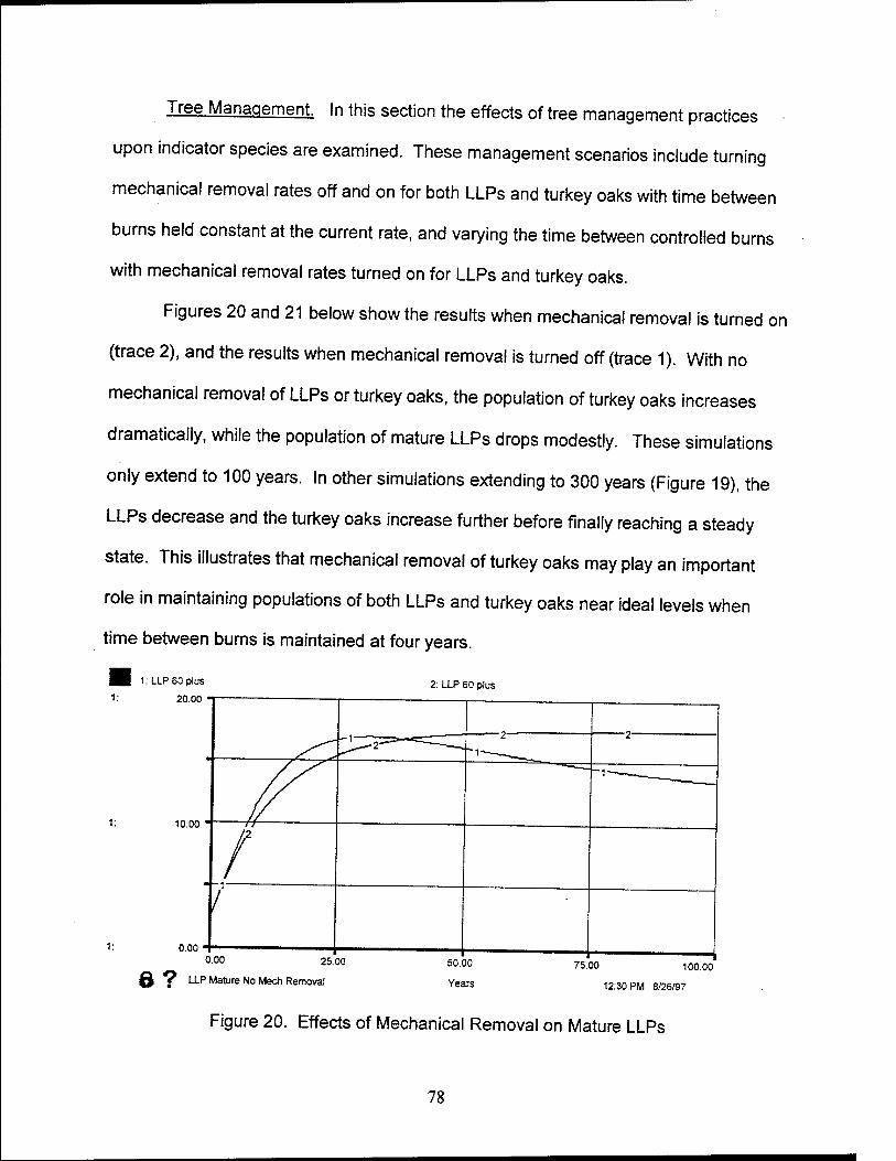
Tree Management. In this section the effects of tree management practices
upon indicator species are examined. These management scenarios include turning
mechanical removal rates off and on for both LLPs and turkey oaks with time between
burns held constant at the current rate, and varying the time between controlled burns
with mechanical removal rates turned on for LLPs and turkey oaks.
Figures 20 and 21 below show the results when mechanical removal is turned on
(trace 2), and the results when mechanical removal is turned off (trace 1). With no
mechanical removal of LLPs or turkey oaks, the population of turkey oaks increases
dramatically, while the population of mature LLPs drops modestly. These simulations
only extend to 100 years. In other simulations extending to 300 years (Figure 19), the
LLPs decrease and the turkey oaks increase further before finally reaching a steady
state. This illustrates that mechanical removal of turkey oaks may play an important
role in maintaining populations of both LLPs and turkey oaks near ideal levels when
time between burns is maintained at four years.
■■ 1:LLP60plus
1: 20.00 t 2: LLP 60 plus
10.00
0.00
Years
100.00
12:30 PM 8/26/97 Q f LLP Mature No Mech Removal
Figure 20. Effects of Mechanical Removal on Mature LLPs
78
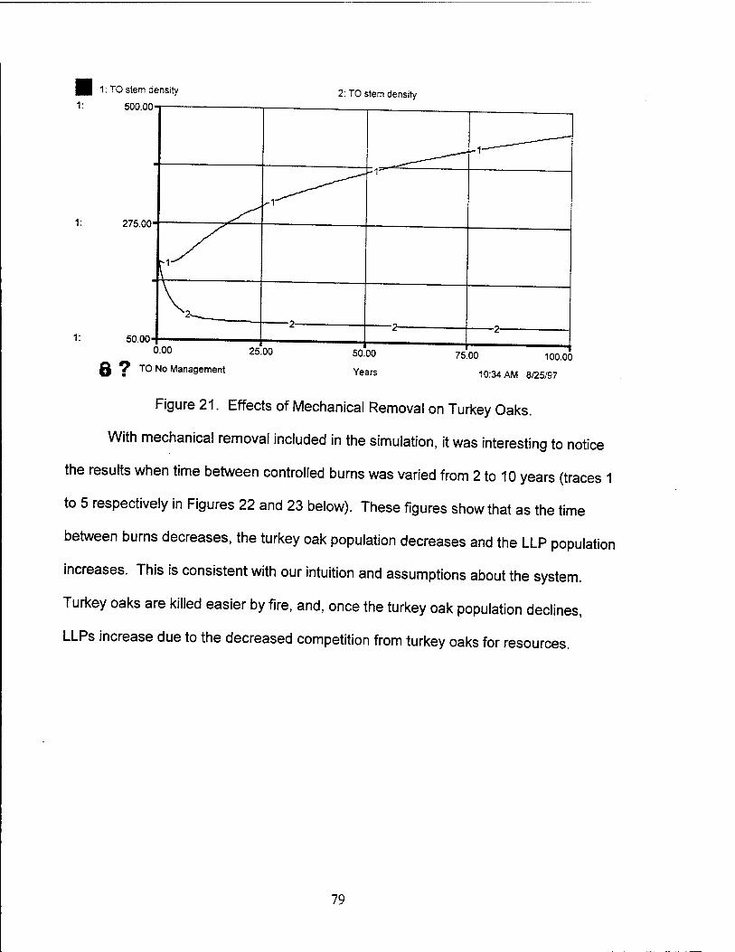
IH 1: TO stem density
1: 500.00-r 2: TO stem density
1: 275.00
50.00 0.00 25.00
Q V TO No Management
50.00
Years
75.00 100.00
10:34 AM 8/25/97
Figure 21. Effects of Mechanical Removal on Turkey Oaks.
With mechanical removal included in the simulation, it was interesting to notice
the results when time between controlled burns was varied from 2 to 10 years (traces 1
to 5 respectively in Figures 22 and 23 below). These figures show that as the time
between burns decreases, the turkey oak population decreases and the LLP population
increases. This is consistent with our intuition and assumptions about the system.
Turkey oaks are killed easier by fire, and, once the turkey oak population declines,
LLPs increase due to the decreased competition from turkey oaks for resources.
79

■ 1:LLP60plus
1: 20.00-r
2: LLP 60 plus 3: LLP 60 plus 4: LLP 60 plus
10.00
0.00 0.00
Q *7 LLP mature
25.00 50.00
Years
75.00 100.00
12:26 PM 8/26/97
Figure 22. LLP Density with Varying Time Between Burns (2, 4, 6, 8, 10 years)
^| 1: TO stem density 2: TO stem density 3: TO stem density 4: TO stem density
1: 200.00T
s: : --j srern cens'tv
132.95"
65.89 0.00
q 7 To Burn
25.00 50.00
Years
75.00 100.00
12:01 PM 8/22/97
Figure 23. Turkey Oak Density with Varying Time Between Burns (2, 4, 6, 8, 10 years)
One weakness of the model is that the fluctuations that occur in tree populations
due to these management practices had almost no effect on RCW population. This
should not be the case. A significant decline in mature LLPs should cause a decline in
80

RCW population. There seems to be a weak link in the model between mature LLP
density and the RCW population stemming from the cavity goodness entity. This model
weakness was discussed at the end of the previous chapter.
A key insight can be gained from comparing the results of no management
(Figure 19), and the results when burn time and mechanical removal are varied. Figure
19 shows that if there is no controlled burning and no mechanical removal, turkey oak
densities reach very high levels, dominating the system, while LLPs decrease
dramatically, to the point of being nearly wiped out. Comparing this to the mechanical
removal results (Figures 20 and 21), where a dramatic increase in turkey oaks can also
be seen when mechanical removal is turned off, it is evident that the turkey oak
population is largely being controlled by mechanical removal instead of burning. This
means that large numbers of turkey oaks must be removed each year to control its
population, which may require significant resource expenditures. On the other hand,
looking at Figures 22 and 23, the model demonstrates that decreasing the time
between burns while mechanical removal is included, the turkey oak population
decreases and LLPs increase. In other results that are not reported, by decreasing the
time between burns to two years while mechanical removal is not included, the turkey
oak population is controlled at levels slightly higher than the baseline. Mature LLPs
also reach higher steady state levels than the baseline scenario (Figure 13). These
results suggest that decreasing the time between burns may be an effective way to
control turkey oaks while maintaining a healthy LLP population. This management
practice has the potential to save resources that would otherwise be spent on turkey
oak mechanical removal.
81
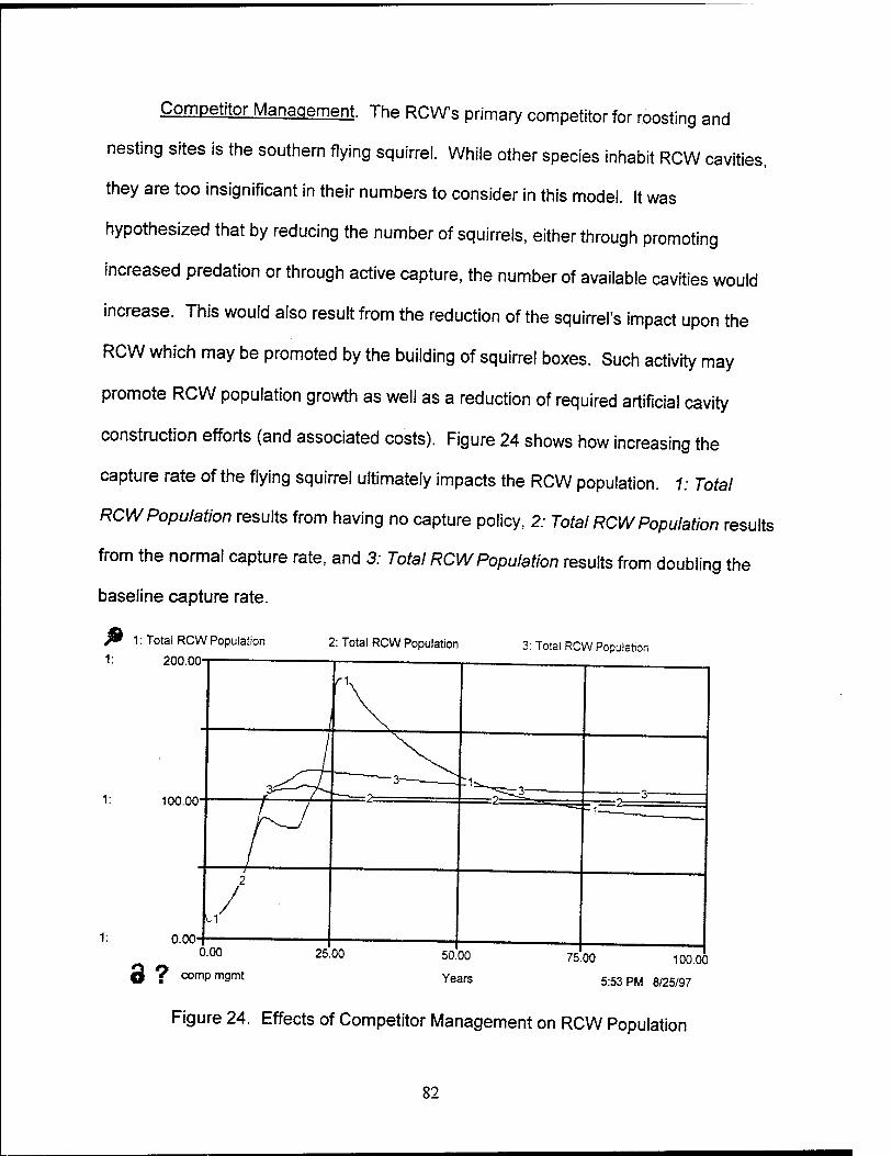
Competitor Management. The RCWs primary competitor for roosting and
nesting sites is the southern flying squirrel. While other species inhabit RCW cavities,
they are too insignificant in their numbers to consider in this model. It was
hypothesized that by reducing the number of squirrels, either through promoting
increased predation or through active capture, the number of available cavities would
increase. This would also result from the reduction of the squirrel's impact upon the
RCW which may be promoted by the building of squirrel boxes. Such activity may
promote RCW population growth as well as a reduction of required artificial cavity
construction efforts (and associated costs). Figure 24 shows how increasing the
capture rate of the flying squirrel ultimately impacts the RCW population. 1: Total
RCW Population results from having no capture policy, 2: Total RCW Population results
from the normal capture rate, and 3: Total RCW Population results from doubling the
baseline capture rate.
7* 1: Total RCW Population
1: 200.00
2: Total RCW Population 3: Total RCW Population
100.00
0.00 0.00
Q V comp mgmt
25.00 50.00
Years
75.00 100.00
5:53 PM 8/25/97
Figure 24. Effects of Competitor Management on RCW Population
82
This graph shows a contradiction to our initial hypothesis that the RCW would be
seriously impacted by the status of the flying squirrel. Having no capture policy shows
an initial reduction in RCW population as there are more squirrels competing for RCW
cavities and cavity construction is slow to respond to the need for more cavities. As the
population of squirrels exhibits overshoot and collapse behavior, brought on by
significant reduction in turkey oaks and squirrel overpopulation, the RCW population
increases to fill the available cavities and then drops to a reasonable and stable
population. Increasing the capture rate, otherwise, has little effect on the size of the
RCW population. Maintaining the squirrel population, whether through predation,
squirrel box construction, or capture, appears to promote stability for the RCW
population; however, in the short run, values from the RCW population are affected
very little through manipulation of squirrel population.
Squirrel predator management may be difficult to control. The promoting of a
current predator or the introduction of new predators may have severe unknown
secondary and tertiary effects upon the environment. If squirrel management practices
are implemented, reduction of cavity competition through the use of boxes, and active
capturing are the preferred management practices.
Based upon these outputs, the active management of the flying squirrel is not
recommended when considering the RCW population alone. Active squirrel
management may, however, reduce the efforts required for artificial cavity construction.
Costs and other resource allocations could determine which is more effective. We
recommend further study of these relationships.
83
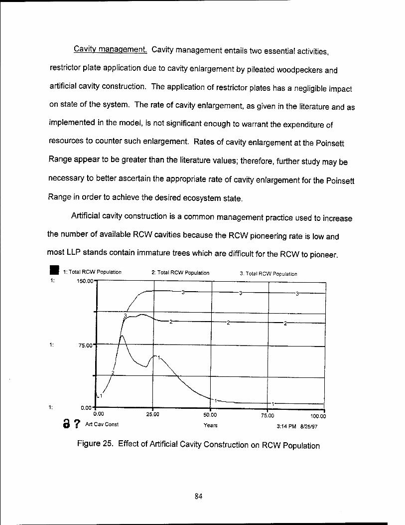
Cavity management. Cavity management entails two essential activities,
restrictor plate application due to cavity enlargement by pileated woodpeckers and
artificial cavity construction. The application of restrictor plates has a negligible impact
on state of the system. The rate of cavity enlargement, as given in the literature and as
implemented in the model, is not significant enough to warrant the expenditure of
resources to counter such enlargement. Rates of cavity enlargement at the Poinsett
Range appear to be greater than the literature values; therefore, further study may be
necessary to better ascertain the appropriate rate of cavity enlargement for the Poinsett
Range in order to achieve the desired ecosystem state.
Artificial cavity construction is a common management practice used to increase
the number of available RCW cavities because the RCW pioneering rate is low and
most LLP stands contain immature trees which are difficult for the RCW to pioneer.
2: Total RCW Population 3: Total RCW Population ■ 1: Total RCW Population
1: 150.00TT
75.00
0.00 0.00
Q f Art Cav Const
25.00 50.00
Years
75.00 100.00
3:14 PM 8/25/97
Figure 25. Effect of Artificial Cavity Construction on RCW Population
84
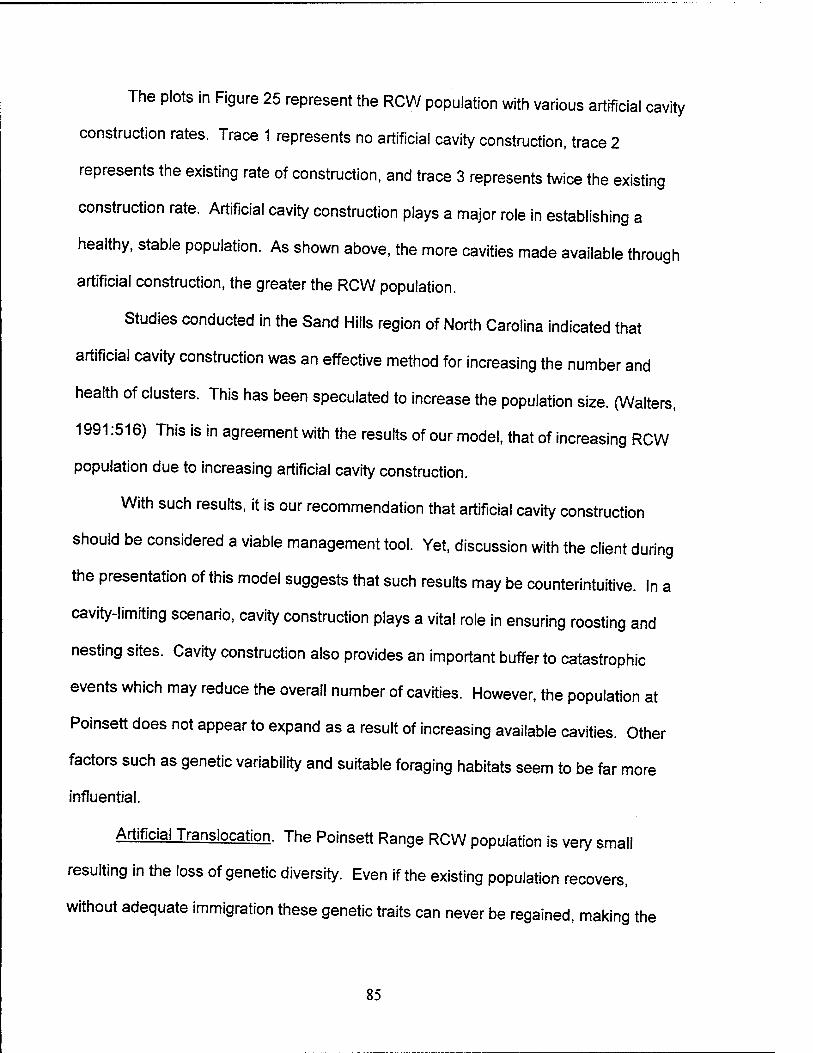
The plots in Figure 25 represent the RCW population with various artificial cavity
construction rates. Trace 1 represents no artificial cavity construction, trace 2
represents the existing rate of construction, and trace 3 represents twice the existing
construction rate. Artificial cavity construction plays a major role in establishing a
healthy, stable population. As shown above, the more cavities made available through
artificial construction, the greater the RCW population.
Studies conducted in the Sand Hills region of North Carolina indicated that
artificial cavity construction was an effective method for increasing the number and
health of clusters. This has been speculated to increase the population size. (Walters,
1991:516) This is in agreement with the results of our model, that of increasing RCW
population due to increasing artificial cavity construction.
With such results, it is our recommendation that artificial cavity construction
should be considered a viable management tool. Yet, discussion with the client during
the presentation of this model suggests that such results may be counterintuitive. In a
cavity-limiting scenario, cavity construction plays a vital role in ensuring roosting and
nesting sites. Cavity construction also provides an important buffer to catastrophic
events which may reduce the overall number of cavities. However, the population at
Poinsett does not appear to expand as a result of increasing available cavities. Other
factors such as genetic variability and suitable foraging habitats seem to be far more
influential.
Artificial Translation. The Poinsett Range RCW population is very small
resulting in the loss of genetic diversity. Even if the existing population recovers,
without adequate immigration these genetic traits can never be regained, making the
85
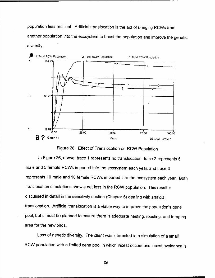
population less resilient. Artificial translocation is the act of bringing RCWs from
another population into the ecosystem to boost the population and improve the genetic
diversity.
?* 1: Total RCW Population
1: 114.43T
2: Total RCW Population 3: Total RCW Population
50.00
Years
75.00 100.00
9:31 AM 22/8/97
Figure 26. Effect of Translocation on RCW Population
In Figure 26, above, trace 1 represents no translocation, trace 2 represents 5
male and 5 female RCWs imported into the ecosystem each year, and trace 3
represents 10 male and 10 female RCWs imported into the ecosystem each year. Both
translocation simulations show a net loss in the RCW population. This result is
discussed in detail in the sensitivity section (Chapter 5) dealing with artificial
translocation. Artificial translocation is a viable way to improve the population's gene
pool, but it must be planned to ensure there is adequate nesting, roosting, and foraging
area for the new birds.
Loss of genetic diversity. The client was interested in a simulation of a small
RCW population with a limited gene pool in which incest occurs and incest avoidance is
86
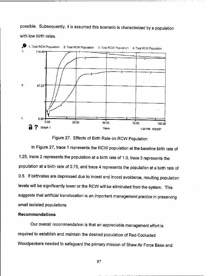
possible. Subsequently, it is assumed this scenario is characterized by a population
with low birth rates.
fi 1: Total RCW Population 2: Total RCW Population 3: Totai RCW Population 4: Tota! RCW Population 1: 114.43T
1: 57.22-
1: 0.00 0.00
0 i Graph 1
25.00 50.00
Years
75.00 100.00
1:25 PM 8/23/97
Figure 27. Effects of Birth Rate on RCW Population
In Figure 27, trace 1 represents the RCW population at the baseline birth rate of
1.25, trace 2 represents the population at a birth rate of 1.0, trace 3 represents the
population at a birth rate of 0.75, and trace 4 represents the population at a birth rate of
0.5. If birthrates are depressed due to incest and incest avoidance, resulting population
levels will be significantly lower or the RCW will be eliminated from the system. This
suggests that artificial translocation is an important management practice in preserving
small isolated populations.
Recommendations
Our overall recommendation is that an appreciable management effort is
required to establish and maintain the desired population of Red-Cockaded
Woodpeckers needed to safeguard the primary mission of Shaw Air Force Base and
87
the Poinsett Weapons Range. More specifically, because sustained management of
the longleaf pine ecosystem has proven to have the greatest contribution to the RCW
habitat, we recommend that active understory management is required to promote this
ecosystem including the burning and/or the mechanical removal of turkey oaks. We
recommend that increasing burning rate (reducing the time between burning) be
implemented. This has the potential to save time and money that would otherwise be
spent on turkey oak mechanical removal.
Artificial RCW translocation also appears to be an effective management tool
and we recommend that these efforts be sustained. In conjunction with appropriate
cavity management, translocation does well to promote genetic diversity thus
strengthening the social interactions, reducing emigration caused by incest avoidance
behavior, and protects the population from disease.
Artificial cavity construction appeared to be a key element in increasing the RCW
population. While current conditions at the Poinsett Range may not support this
hypothesis, the literature and the model output do. As a result, we recommend that
active construction be considered and that there be further study and modeling of the
relationships between LLPs, RCW cavity construction, cluster dynamics, and
roosting/nesting behavior.
88

VII. Conclusions
Research Questions Answered
1. How is the number of RCW clusters affected by environmental factors and
management practices? - It was determined the number of RCW clusters are
influenced by the artificial cavity construction rate and the availability of acceptable
cavities. Negligible effects were observed from foraging area impacts.
2. What are the impacts on the longleaf pine ecosystem viability if habitat management
is driven by RCW population goals? - It was determined that the RCW and longleaf
pine management goals are not contradictory. Managing to provide an optimum
longleaf pine ecosystem provides the RCW with the necessary habitat for foraging
and cavity construction.
3. What management practices will be required to restore and to maintain a longleaf
pine ecosystem? - A combination of mechanical removal and burning yield the more
viable longleaf pine ecosystem. Concentrating on decreasing the time between
burning will reduce mechanical removal requirements, which may be more cost
effective.
4. How much human resource expenditure with regard to management practices is
required to maintain a stable ecosystem? - The model demonstrated some effort is
required to maintain low turkey oak population which ensures an acceptable
longleaf pine population. Due to the low pioneering rate of the RCW, management
effort will also be required to maintain the appropriate number of acceptable cavities.
89
5. What are the effects of management practices on the indicator species? - The
current management practices will decrease the number of turkey oaks, improve
longleafpine age structure, and increase the RCWpopulation.
Suggestions for Further Study
Although the project model captures a majority of the critical mechanisms of the
Poinsett Range ecosystem, several areas which could play a significant role in
determining the ecosystem's behavior over time have not been included in the current
model or been explored in depth. Some of these areas have already been mentioned
as model weaknesses (and should be studied further to address those model
weaknesses), so they will not be discussed again. In future efforts to model the
Poinsett Range ecosystem, these areas may offer greater insight into the entities and
interactions driving the behavior actually seen in the ecosystem and provide a client
with a better tool for ecosystem management.
Other Indicator Species. Several different types of species can be utilized to
ascertain the health of a particular ecosystem. These indicator species are sensitive to
changes occurring in the state of the ecosystem and, consequently, are used to
determine the'health of the ecosystem. Although the current model contains several
indicator species (longleaf pine, turkey oak, squirrels, and RCW), it does not include
other species such as wire grass and bobwhite quail which could also be influential in
determining the health of the Poinsett Range ecosystem.
Effects of Various Soil Types. Conditions necessary for certain species of trees
to thrive were not comprehensively discussed or utilized in constructing the model. The
most notable condition which was not pursued is soil condition. Various soil types will
90
significantly impact the level and type of vegetation supported in the ecosystem and,
consequently, the heterogeneity of the area and overall diversity of the ecosystem. Soil
conditions are especially critical when a particular species such as the longleaf pine is
desired. Soil conditions conducive to longleaf pine growth may not support other types
of vegetation which play a vital role in the overall range ecosystem. Soil conditions may
also limit the choice of strategies available in managing the ecosystem.
Management Strategy Cost Benefit Analysis Despite numerous types of
management practices and their combinations being explored through model simulation
to analyze the long-term implications of these practices on the ecosystem, no
cost/benefit limitations were placed on the strategies employed. Clearly each of the
tested management scenarios has an associated cost. These costs may prove to be
the determining factor on which practices could be utilized for managing the Poinsett
Range. However, along with the expense of various practices, the benefit received
from using a particular strategy should also be weighed to ensure the best management
practice is pursued in creating the desired ecosystem state.
The project does not address either of these areas when analyzing long-term
simulations for making recommendations about particular management practices.
Management scenarios were simulated regardless of the cost involved; however, cost
analysis would not alter the management practice's effect on the ecosystem, only the
practice selected by the client. Benefits for the ecosystem are derived from the model
output for each scenario but are not viewed in conjunction with cost. Costs and the
relationship between cost and benefits must be incorporated into future efforts if the
91

client wishes to utilize the model in determining the most effective strategy for
managing the Poinsett Range ecosystem given a limited amount of resources.
92
Bibliography
Barlow, Chuck D. "The Proposed Management of the Red-Cockaded Woodpecker in the Southern National Forests: Analysis and Suggestions " UALR Law Journal. 17: 727-764(1995).
Bonnie, Robert. "Safe Harbor," Journal of Forestry. 95: 17-22(1997).
Conner, Richard N., D. Craig Rudolph, David L. Kulhavy, and Ann E. Snow "Causes of Mortality of RCW Cavity Trees," Journal of Wildlife Management 5S- ooT-oo/ (iyy 1).
Conner, Richard N., D. Craig Rudolph, Danial Saenz, and Richard R. Shaefer. "Heartwood, Sapwood, and Fungal Decay Associated with RCW Cavity Tress " Journal of Wildlife Management. 58: 728-734(1994).
Conner, Richard N. and D. Craig Rudolph. "Losses of Red-Cockaded Woodpecker Cavity Trees to Southern Pine Beetles," Wilson Bulletin. 107: 81-92 (1995).
Conner, R. N., D. Craig Rudolph, and Larry H. Bonner. "Red-Cockaded Woodpecker Population Trends and Management on Texas National Forests," Journal of Field Ornithology. 66(1): 140-151 (1995).
Conner, Richard N. and Craig Rudolph. "RCW Use of Seed-Tree/Shelterwood Cuts in Eastern Texas," Wildlife Society Bulletin, 1QMV 67-73(1991).
Copeyon, Carole K., Jeffery R. Walters, and J. H. Carter III. "Induction of Red- Cockaded Woodpecker Group Formation by Artificial Cavity Construction " Journal of Wildlife Management. 55: 54Q-55fi MQQI)
DeLotelle, R. S. and R. J. Epting. "Reproduction of the Red-Cockaded Woodpecker in Central Florida." Wilson Bull.. 104: 285-294 (1992).
Edwards, John W, Ernest E. Stevens, and Charles A. Dachelet. "Insert Modifications Improve Access to Artificial RCW Nest Cavities," Journal of Field Ornitholoov 68(2): 228-234(1997). aXl"
Engstrom, L. A. Brennan, W. L. Neel, R. M. Farrar, S. T. Lindeman, W. K. Moser and S. M. Herman. "Silvicultural Practices and RCW Management: A Reply to Conner and Rudolph," Wildlife Society Bulletin. 24(2): 334-338 (1996).
Everhart, S.H., P.D. Doerr, and J.R. Walters, "Snag Density and Interspecific Use of RCW Cavities" The Journal of the Elisha Mitchell Scientific SnrtPtv 109(1)- 37- 44(1993). ~~~ * LLi'
93
Forrester, Jay W. and Peter M. Senge. "Test for Building Confidence in System Dynamics Models," in Modeling For Management II: Simulation in Support of Systems Thinking. Ed. George P. Richardson. Brookfield, VT: Dartmouth Publishing Company, 1996.
Gordon, Steven I. Computer Models in Environmental Planning. New York: Van Nostrand Reinhold Company, 1985.
Hanula, James L. and Kathleen E. Franzreb. "Arthropod Prey of Nestling Red- Cockaded Woodpeckers in the Upper Coastal Plain Of South Carolina," The Wilson Bulletin. 107(3): 485-495(1995).
Harlow, Richard F. "Food Habits of Southern Flying Squirrels (Glaucomys volans) Collected from RCW (Picoides borealis) Colonies in South Carolina," The American Midland Naturalist. 124: 187-191 (1990).
Harlow, William M. and Harrar, Ellwood S. Textbook of Dendrology. New York: McGraw-Hill, Inc., 1958.
Harlow, William M. and others. Textbook of Dendrology. 8th Edition. New York: McGraw-Hill, Inc., 1996.
Harrar, Ellwood S. and Harrar, J. George. Guide to Southern Trees. New York: Dover Publications, Inc., 1962.
Hooper, Robert G., L. J. Niles, and R. F. Harlow. "Home Ranges of Red- Cockaded Woodpeckers in Coastal South Carolina," Auk. 99: 675-682 (1982).
Hooper, Robert G.. "Arthropod Biomass in Winter and the Age of Longleaf Pine." Forest Ecology and Management. 82: 115-131 (1996).
Hooper, Robert G. "Longleaf Pines Used for Cavities by Red-Cockaded Woodpeckers," Journal of Wildlife Management. 52: 392-398(1988).
Jackson, Jerome A. "The Evolution, Taxonomy, Distribution, Past Populations, and Current Status of the Red-Cockaded Woodpecker," in R. L. Thompson, ed. "The Ecology and Management of the Red-Cockaded Woodpecker," US Bureau of Sport. Fish. And Wildlife, and Tall Timbers Res. Stm.. Tallahassee, FL (1971).
Jackson, Jerome A., Michael R. Lennartz, and Robert G. Hooper. "Tree Age and Cavity Initiation by RCWs," Journal of Forestry: 102-103 (February 1979).
94
Jackson, Jerome A. "The Red-Cockaded Woodpecker Recovery Program," in Endangered Species Recovery. Ed. by Tim W. Clark, Richard P. Reading, and Alice L. Clarke. Island Press, Washington D.C.: 1994.
Kelly, Jeffery F., Sandra M. Pletschet, and David M. Leslie, Jr. "Habitat Associations of RCW Cavity Trees in an Old-Growth Forest of Oklahoma," Journal of Wildlife Management. 57: 122-128(1993).
Lennartz, M. R. and Gary V. Henry. Endangered Species Recovery Plan - Red Cockaded Woodpecker (Picaides borealis). U. S. Fish and Wildlife Service, Region 4. Atlanta, GA: Government Printing Office, 11 Apr 1985.
Lennartz, M. R., R. G. Hooper, and R. F. Harlow. "Sociality and Cooperative Breeding of the Red-Cockaded Woodpecker, (Picaides borealis)" Behav. Ecol. Sociobiol.. 20: 77-88(1987).
Loeb, Susan C. "Use and Selection of RCW Cavities by Southern Flying Squirrels," Journal of Wildlife Management. 57: 329-335(1993).
Ligon, J. D. "Behavior and Breeding Biology of the Red-Cockaded Woodpecker," Auk. 87: 255-278(1970).
McGinty, Douglas T. and E. Jennifer Christy. "Turkey Oak Ecology on a Georgia Sandhill," The American Midland Naturalist. 98: 487-491(1977).
Morecroft, John D. "System Dynamics and Microworlds for Policy Makers," in Modelling for Management II: Simulation in Support of Systems Thinking. Ed. George P. Richardson. Brookfield, VT: Dartmouth Publishing Company, 1996.
Peters, Robert L. "Hope for the Red-Cockaded?," Defenders. 71: 21-32 (1996).
Platt, William J., Gregory W. Evans, and Stephen L. Rathburn. "The Population Dynamics of a Long-Lived Conifer (Pinus palustris)," The American Naturalist. 131(4): 491-525 (April 1988).
Porter, M. I. and R. F. Labisky. "Home Range and Foraging Habitat of Red-Cockaded Woodpeckers in Northern Florida," J. Wildl. Manage.. 50: 239-247 (1986).
Pyne, Stephen J. and others. Introduction to Wildland Fire. 2nd Edition. New York: John Wiley and Sons, Inc., 1996.
Rebertus, Alan J., G. Bruce Williamson, and E. Barry Moser. "Longleaf Pine Pyrogenicity and Turkey Oak Mortality in Florida Xeric Sandhills," Ecology. 7Q- 60-70(1989).
95
Roise, Joseph, Joosang Chung, Richard Lancia, and Mike Lennartz. "Red-Cockaded Woodpecker Habitat and Timber Management: Production Possibilities," Southern Journal of Applied Forestry. 14(1): 6-12(1990).
Rogers, Stan. Wildlife Biologist, EIAP Manager. Personal Correspondence (Electronic Mail). 4 August 1997.
Ross, W. G., D. L. Kulhavy, and R. N. Conner. "Stand Conditions and Tree Characteristics Affect Quality of Longleaf Pine for RCW Cavity Trees," Forest Ecology and Management. 91: 145-154(1997).
Rosseil, C. Reed, Jr. and Bryan Gorsira. "Assessment of Condition and Availability of Active RCW Cavities," Wildlife Society Bulletin. 24: 21-24 (1996).
Rudolph, D. Craig and Richard N. Conner. "Cavity Tree Selection by Red-Cockaded Woodpeckers in Relation to Tree Age," The Wilson Bulletin. 103C3V 458-467 (1991).
Rudolph, D. Craig and Richard N. Conner. "Forest Fragmentation and Red-Cockaded Woodpecker Population: An Analysis at Intermediate Scale," Journal of Field Ornithology. 65(3): 365-375(1994).
Rudolph, D. Craig, Richard N. Conner, and Janet Turner. "Competition for Red- Cockaded Woodpecker Roost and Nest Cavities: Effects of Resin Age and Entrance Diameter," The Wilson Bulletin. 102: 23-36 (1990).
Rudolph, D., Howard Kyle, and Richard N. Conner. "Red-Cockaded Woodpeckers Vs. Rat Snakes; The Effectiveness of the Resin Barrier "The Wilson Bulletin. 102: 14-22(1990).
Sargent, Charles Sprague. Manual of the Trees of North America. New York: Dover Publications, Inc., 1965.
Sawyer, Sherrie L. and Robert K. Rose. "Homing in and Ecology of the Southern Flying Squirrel Glaucomys volans in Southeastern Virginia," The American Midland Naturalist. 113: 238-243(1985).
Shaw Air Force Base Natural Resources Manager. RCW Management Plan for Poinsett Weapons Range. ShawAFB, February 1995.
Shaw Air Force Base Natural Resources Management Division. Forestry Management Plan for Shaw Air Force Base. South Carolina. ShawAFB, October 1996.
Shelley, M.L. Class handout, ENVR 775, Strategic Environmental Management. Air Force Institute of Technology, Wright Patterson AFB OH, Summer Quarter 1996.
96
Sterman, John D. "Learning in and about complex systems," in Modelling for Management II: Simulation in Support of Systems Thinking Ed. George P Richardson. Brookfield, VT: Dartmouth Publishing Company, 1996.
Stone, Karen D., Gary A. Heidt, Paul T. Caster, and Michael L. Kennedy. "Using Geographic Information Systems to Determine Home Range of the Southern Flying Squirrel (Glaucomys volans)," The American Midland Naturalist 137- 106-111(1997). " ' '
Thomlinson, John R. "Predicting Status Change in RCW Cavity-Tree Clusters" Journal of Wildlife Management. 60: 350-354(1996). '
U.S. Fish and Wildlife Service. Red-Cockaded Woodpecker Recovery Plan Atlanta, GA: U.S. Fish and Wildlife Service, 1985.
Wahlenberg, W. G. Lonoleaf Pine. Washington, D. C: Charles Lathrop Pack Forestry Foundation, 1946.
Walters, J. R., P. D. Doerr, and J. H. Carter. The Cooperative Breeding System of the Red-Cockaded Woodpeckers," Ethology.. 78- 275-305 (1988). —
Walters, J.R. "RCWs: a 'Primitive' Cooperative Breeder," in Cooperative Breeding in Birds. Ed. Peter B. Stacey and Walter D. Koenig. Cambridge: Cambridge University Press, 1991.
Ware, Stewart and others. "Southern Mixed Hardwood Forest: The Former Longleaf Pine Forest," in Biodiversity of the Southeastern United States New York: John Wiley and Sons, Inc., 1993.
Wells-Gosling, Nancy. Flying Souirrels. Gliders in the Dark Smithsonian Institute Press, 1985.
97
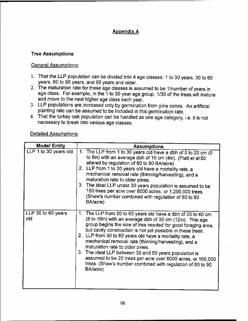
Appendix A
Tree Assumptions
General Assumptions:
1. That the LLP population can be divided into 4 age classes: 1 to 30 years, 30 to 60 years, 60 to 95 years, and 95 years and older.
2. The maturation rate for these age classes is assumed to be 1/number of years in age class. For example, in the 1 to 30 year age group, 1/30 of the trees will mature and move to the next higher age class each year.
3. LLP populations are increased only by germination from pine cones. An artificial planting rate can be assumed to be included in this germination rate.
4. That the turkey oak population can be handled as one age category, i.e. it is not necessary to break into various age classes.
Detailed Assumptions:
Model Entity LLP 1 to 30 years old
Assumptions
LLP 30 to 60 years old
1. The LLP from 1 to 30 years old have a dbh of 0 to 20 cm (0 to 8in) with an average dbh of 10 cm (4in). (Platt et al:50 altered by regulation of 60 to 90 BA/acre)
2. LLP from 1 to 30 years old have a mortality rate, a mechanical removal rate (thinning/harvesting), and a maturation rate to older pines.
3. The ideal LLP under 30 years population is assumed to be 150 trees per acre over 8000 acres, or 1,200,000 trees. (Shaw's number combined with regulation of 60 to 90 BA/acre)
1.
3.
The LLP from 30 to 60 years old have a dbh of 20 to 40 cm (8 to 16in) with an average dbh of 30 cm (12in). This age group begins the size of tree needed for good foraging area, but cavity construction is not yet possible in these trees. LLP from 30 to 60 years old have a mortality rate, a mechanical removal rate (thinning/harvesting), and a maturation rate to older pines. The ideal LLP between 30 and 60 years population is assumed to be 20 trees per acre over 8000 acres, or 160,000 trees. (Shaw's number combined with regulation of 60 to 90 BA/acre)
98
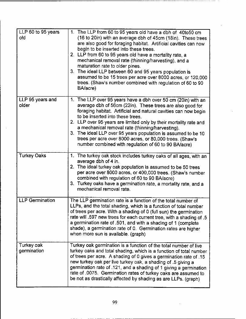
LLP 60 to 95 years old
1. The LLP from 60 to 95 years old have a dbh of 40to50 cm (16 to 20in) with an average dbh of 45cm (18in). These trees are also good for foraging habitat. Artificial cavities can now begin to be inserted into these trees.
2. LLP from 60 to 95 years old have a mortality rate, a mechanical removal rate (thinning/harvesting), and a maturation rate to older pines.
3. The ideal LLP between 60 and 95 years population is assumed to be 15 trees per acre over 8000 acres, or 120,000 trees. (Shaw's number combined with regulation of 60 to 90 BA/acre)
LLP 95 years and older
1. The LLP over 95 years have a dbh over 50 cm (20in) with an average dbh of 56cm (22in). These trees are also good for foraging habitat. Artificial and natural cavities can now begin to be inserted into these trees.
2. LLP over 95 years are limited only by their mortality rate and a mechanical removal rate (thinning/harvesting).
3. The ideal LLP over 95 years population is assumed to be 10 trees per acre over 8000 acres, or 80,000 trees. (Shaw's number combined with regulation of 60 to 90 BA/acre)
Turkey Oaks 1. The turkey oak stock includes turkey oaks of all ages, with an average dbh of 4 in.
2. The ideal turkey oak population is assumed to be 50 trees per acre over 8000 acres, or 400,000 trees. (Shaw's number combined with regulation of 60 to 90 BA/acre)
3. Turkey oaks have a germination rate, a mortality rate, and a mechanical removal rate.
LLP Germination The LLP germination rate is a function of the total number of LLPs, and the total shading, which is a function of total number of trees per acre. With a shading of 0 (full sun) the germination rate will .597 new trees for each current tree, with a shading of .5 a germination rate of .501, and with a shading of 1 (complete shade), a germination rate of 0. Germination rates are higher when more sun is available, (graph)
Turkey oak germination
Turkey oak germination is a function of the total number of live turkey oaks and total shading, which is a function of total number of trees per acre. A shading of 0 gives a germination rate of .15 new turkey oak per live turkey oak, a shading of .5 giving a germination rate of .121, and a shading of 1 giving a germination rate of .0075. Germination rates of turkey oaks are assumed to be not as drastically affected by shading as are LLPs. (graph)
99

Turkey Oak Resprout
Shading
LLP Shading
Turkey Oak Shading
LLP Natural Mortality Rate
LLP 1 to 30 Natural Mortality
LLP 30 to60 Natural Mortality
LLP 60 to 95 Natural Mortality
LLP 95+ Natural Mortality
Turkey Oak Natural Mortality
It is assumed that 67% of the turkey oaks that die as a result of burning will resprout.
Shading by living trees is assumed to affect the successful germination of both LLPs and turkey oaks. This is a factor that vanes form 0 to 1 based upon the density of turkey oaks and of LLPs, with turkey oaks having the greater impact on shading (maximum value of .7), while the LLPs have less of an impact (maximum value of .3).
LLP shading is a function of LLP density with 0 trees per acre having a shading of .0015 and 300 trees per acre having a shading of .3. LLP density is the sum of all LLPs (all aqes) divided by the total area, (graph)
Turkey oak shading is a function of turkey oak density with 0 trees per acre having a shading of .0 and 1000 trees per acre having a shading of .7. (graph)
Natural mortality varies inversely with total tree health and is different for the four age groups of LLP. Baseline intrinsic mortality rates came from Platt et al (500.), and were used in determining the dynamic death rates, (graph)
For LLP less than 30 years, when tree health is .2, the natural mortality is .099 while when the tree health is 1 the natural mortality is .01.
For LLP between 30 and 60 years, when tree health is 0 the natural mortality is .01 while when the tree health is 1 the natural mortality is .001.
For LLP between 60 and 95 years, when tree health is 0 the natural mortality is .00995 while when the tree health is 1 the natural mortality is .001.
For LLP greater than 95 years, when tree health is 0, the natural mortality is .0496 while when the tree health is 1 the natural mortality is .00545.
For the turkey oaks, assuming the average age is 40 years the natural mortality varies with total basal area per acre with a density maximized at 150 having a mortality rate of .0498 and a density of 0 having a mortality rate of 0.
100

LLP Tree Health general
Burn Health
Mechanical Removal Health
Mechanical Removal of Trees
LLP 1 to 30 Mech. Rem. Health
LLP 30 to 60 Mech. Rem. Health
LLP 60 to 95 Mech. Rem. Health
LLP 95+ Mech. Rem. Health
Tree health varies with the burn health, the mechanical removal health, and the basal area health, weighted .1, 3 and 6 respectively.
The burn health for each tree group is a function of the burn time, with a burn time of 4 years giving a maximum burn health and the burn health decreasing if the burn time increases or decreases. The burn time is set at a constant value of 4 years but can be altered to explore different management practices ' The values are similar for each group of trees.
The mechanical removal health is a function of the removal rate per area for each group of trees. The removal rate is the excess trees divided by the time between thinning, which is set at 8 years for the LLPs and 4 years for the turkey oaks. The excess trees are the difference between the ideal stem density and the actual stem density. Note that if the ideal is greater than the actual, then no mechanical removal will occur.
The mechanical removal rate for LLP represent thinning for pulpwood, while for the turkey oaks it represents clearing all hardwoods in the area. We assume the trees with weaker health will be removed, and any removal will increase the health of the entire stand.
For the LLP less than 30 years, a mechanical removal rate of 0 has a mechanical removal health of .005 while a mechanical removal rate of 5 has a mechanical removal health of 1. (graph)
For the LLP between 30 and 60 years, a mechanical removal rate of 0 has a mechanical removal health of .015 while a mechanical removal rate of 1 has a mechanical removal health of 1. (graph)
For the LLP between 60 and 95 years, a mechanical removal rate of 0 has a mechanical removal health of .01 while a mechanical removal rate of .5 has a mechanical removal health of 1. (graph)
For the LLP greater than 95 years, a mechanical removal rate of 0 has a mechanical removal health of .005 while a mechanical removal rate of 1 has a mechanical removal health of 995 (graph)
101
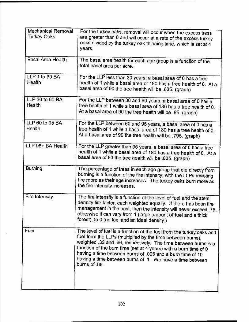
Mechanical Removal Turkey Oaks
Basal Area Health
LLP 1 to 30 BA Health
For the turkey oaks, removal will occur when the excess tress are greater than 0 and will occur at a rate of the excess turkey oaks divided by the turkey oak thinning time, which is set at 4 years.
The basal area health for each age group is a function of the total basal area per acre.
LLP 30 to 60 BA Health
LLP 60 to 95 BA Health
For the LLP less than 30 years, a basal area of 0 has a tree health of 1 while a basal area of 180 has a tree health of 0. At a basal area of 90 the tree health will be .835. (graph)
For the LLP between 30 and 60 years, a basal area of 0 has a tree health of 1 while a basal area of 180 has a tree health of 0. At a basal area of 90 the tree health will be .85. (graph)
LLP 95+ BA Health
Burning
For the LLP between 60 and 95 years, a basal area of 0 has a tree health of 1 while a basal area of 180 has a tree health of 0. At a basal area of 90 the tree health will be .795. (graph)
For the LLP greater than 95 years, a basal area of 0 has a tree health of 1 while a basal area of 180 has a tree health of 0. At a basal area of 90 the tree health will be .835. (graph)
Fire Intensity
The percentage of trees in each age group that die directly from burning is a function of the fire intensity, with the LLPs resisting fire more as their age increases. The turkey oaks burn more as the fire intensity increases.
Fuel
The fire intensity is a function of the level of fuel and the stem density fire factor, each weighted equally. If there has been fire management in the past, then the intensity will never exceed .75, otherwise it can vary from 1 (large amount of fuel and a thick forest), to 0 (no fuel and an ideal density.)
The level of fuel is a function of the fuel from the turkey oaks and fuel from the LLPs (multiplied by the time between burns), weighted .33 and .66, respectively. The time between burns is a function of the bum time (set at 4 years) with a burn time of 0 having a time between bums of .005 and a burn time of 10 having a time between burns of 1. We have a time between burns of .69.
102
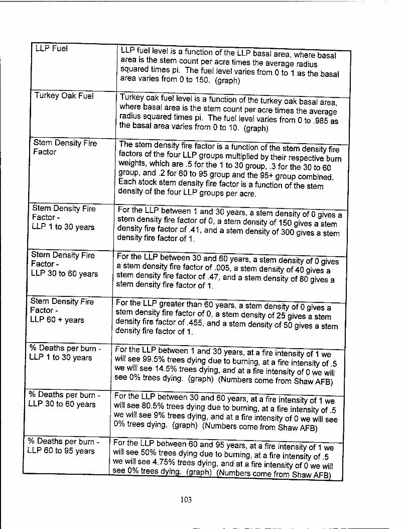
LLP Fuel
Turkey Oak Fuel
Stem Density Fire Factor
Stem Density Fire Factor - LLP 1 to 30 years
Stem Density Fire Factor - LLP 30 to 60 years
Stem Density Fire Factor - LLP 60 + years
% Deaths per burn LLP 1 to 30 years
% Deaths per burn LLP 30 to 60 years
% Deaths per burn LLP 60 to 95 years
LLP fuel level is a function of the LLP basal area, where basal area is the stem count per acre times the average radius squared times pi. The fuel level varies from 0 to 1 as the basal area varies from 0 to 150. (graph)
Turkey oak fuel level is a function of the turkey oak basal area where basal area is the stem count per acre times the average radius squared times pi. The fuel level varies from 0 to 985 as the basal area varies from 0 to 10. (graph)
The stem density fire factor is a function of the stem density fire factors of the four LLP groups multiplied by their respective burn weights, which are .5 for the 1 to 30 group, .3 for the 30 to 60 group, and .2 for 60 to 95 group and the 95+ group combined Each stock stem density fire factor is a function of the stem density of the four LLP groups per acre.
For the LLP between 1 and 30 years, a stem density of 0 gives a stem density fire factor of 0, a stem density of 150 gives a stem density fire factor of .41, and a stem density of 300 gives a stem density fire factor of 1.
For,the LLP between 30 and 60 years, a stem density of 0 gives a stem density fire factor of .005, a stem density of 40 gives a stem density fire factor of .47, and a stem density of 80 qives a stem density fire factor of 1
F°r the LLP greater than 60 years, a stem density of 0 gives a stem density fire factor of 0, a stem density of 25 gives a stem density fire factor of .455, and a stem density of 50 gives a stem density fire factor of 1.
F°r the LLP between 1 and 30 years, at a fire intensity of 1 we will see 99.5% trees dying due to burning, at a fire intensity of 5 we will see 14.5% trees dying, and at a fire intensity of 0 we will see 0% trees dying, (graph) (Numbers come from Shaw AFB)
For the LLP between 30 and 60 years, at a fire intensity of 1 we will see 80.5% trees dying due to burning, at a fire intensity of 5 we will see 9% trees dying, and at a fire intensity of 0 we will see 0/o trees dying, (graph) (Numbers come from Shaw AFB)
n c£, een 60 and 95 years- at a fire intensity of 1 we will see 50% trees dying due to burning, at a fire intensity of 5 we will see 4.75% trees dying, and at a fire intensity of 0 we will see 0% trees dying, (graph) (Numbers come from Shaw AFB)
103

% Deaths per burn - LLP 95 and older
For the LLP greater than 95 years, at a fire intensity of 1 we will see 29.9% trees dying due to burning, at a fire intensity of .5 we will see 5.5% trees dying, and at a fire intensity of 0 we will see 0% trees dying, (graph) (Numbers come from Shaw AFB)
% Deaths per burn - Turkey oaks
For turkey oaks, at a fire intensity of 1 we will see 90% trees dying due to burning, at a fire intensity of .5 we will see 25.5% trees dying, and at a fire intensity of 0 we will see 0% trees dying, (graph) (Numbers come from Shaw AFB)
Ips Beetle Infestation Ips beetle infestation is a function of total tree health for each group of LLPs. When the total health varies from .2 to 1, the Ips beetle infestation factor varies from .02 to .002. Beetle infestation rates are assumed to be the same for each tree age category. (Graphs)
Southern Pine Beetle Infestation
The southern pine beetle infestation is a function of total tree health for each group of LLPs. When total health is 0, the infestation rate is .905. The rate drops off until it reaches 0 when total health equals .4. The rate remains at 0 while the total health varies from .4 to 1. Beetle infestation rates are assumed to be the same for each tree age category. (Graphs)
Cavity Assumptions
General Assumptions:
3.
4.
The number of acceptable available cavities (Acpt Avail Cav) is the primary unit of interest. The flow into the Acpt Avail Cav node has inflow of cavity construction (Cavity Const Rate), an outflow of cavity tree loss, and biflows of RCW occupied cavities (RCW Cav Ocp), Squirrel occupied cavities (Squir Cav Ocp), and cavities made unacceptable through enlargement (Unacpt Cavity). Total number of cavities consists of Total Cav = Acpt Avail Cav + RCW Cav Ocp + Squir Cav Ocp + Unacpt Cavity. When a cavity dies, its occupant automatically fills another available cavity.
Detailed Assumptions:
Model Entity Assumptions Acpt Avail Cav This stock increases with cavity construction and as cavities are
given up by occupants. It decreases as cavities are occupied or enlarged.
104

Art Cavity Rate
Pioneering Rate
The maximum rate is 20 per year. The rate is a function of existing available cavities. As available cavities decrease the artificial cavity rate increases.
The maximum rate is 3 per year. The rate is a function of existing available cavities. As available cavities decrease the pioneering rate increases.
LLP Find Rate
Total Cav
Cavity Tree Loss
This conceptualizes the chance of a RCW finding an acceptable tree to pioneer. If there are many, the chances are good, if there are few, the chances are slim.
This is an aggregate of acceptable and unacceptable cavity trees
This is the loss of cavity trees via an increased mortality due to the weakening of the infrastructure as a result of cavities. It is inclusive of RCW, squirrel, and acceptable cavity loss. A "resident" occupies another cavity if the tree dies. Cavities will be reoccupied unless made unacceptable.
RCW Ocp Rate (biflow) Squir Ocp Rate (biflow)
Competition Pressure
Frac N Cav
Competition Birth Rate
This is equivalent to RCW pop change.
This is equivalent to the squirrel competition pressure value.
(Birth - death - capture) * fraction - squirrel box rate. Squirrel population change times fraction living in cavities less the number of squirrels boxes installed each year yields change in cavity occupancy per year.
Fraction of squirrels that occupy RCW cavities = 0.67.
Food Factor
TO Basal-area
Capture\mort_rate
According to (Sawyer: 1985) squirrels have two litters per year of about 2.5 squirrels per litter. Therefore, each breeding pair would produce 5 squirrels per year and each squirrel would produce 2.5 squirrels per year. Since all squirrels are not of breeding age we assume a birth rate of 2 squirrels per squirrel per year.
A limiting factor on squirrel birth rate which is a function of turkey oak density. Turkey oaks provide acorns which is squirrel primary food source.
Uses turkey oak density to determine optimum foraging conditions (Food per Squirrel) and protection via cover (Predation Rate)
This is a combination of natural mortality rate and the management practice of capturing squirrels.
105
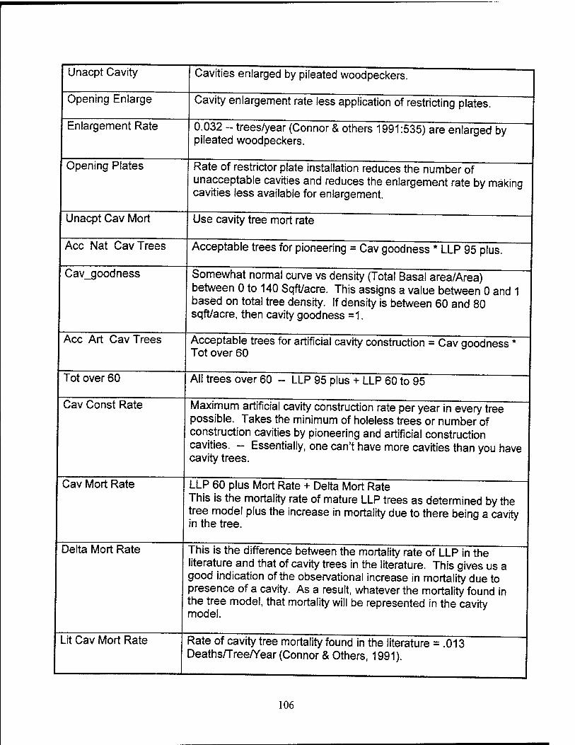
Unacpt Cavity
Opening Enlarge
Enlargement Rate
Opening Plates
Cavities enlarged by pileated woodpeckers.
Cavity enlargement rate less application of restricting plates.
0.032 - trees/year (Connor & others 1991:535) are enlarged by pileated woodpeckers.
Unacpt Cav Mort
Ace Nat Cav Trees
Cav_goodness
Rate of restrictor plate installation reduces the number of unacceptable cavities and reduces the enlargement rate by making cavities less available for enlargement.
Use cavity tree mort rate
Acceptable trees for pioneering = Cav goodness * LLP 95 plus.
Ace Art Cav Trees
Tot over 60
Cav Const Rate
Somewhat normal curve vs density (Total Basal area/Area) between 0 to 140 Sqft/acre. This assigns a value between 0 and 1 based on total tree density. If density is between 60 and 80 sqft/acre, then cavity goodness =1.
Acceptable trees for artificial cavity construction = Cav goodness Tot over 60
All trees over 60 - LLP 95 plus + LLP 60 to 95
Cav Mort Rate
Delta Mort Rate
Maximum artificial cavity construction rate per year in every tree possible. Takes the minimum of holeless trees or number of construction cavities by pioneering and artificial construction cavities. ~ Essentially, one can't have more cavities than you have cavity trees.
LLP 60 plus Mort Rate + Delta Mort Rate This is the mortality rate of mature LLP trees as determined by the tree model plus the increase in mortality due to there being a cavity in the tree.
Lit Cav Mort Rate
This is the difference between the mortality rate of LLP in the literature and that of cavity trees in the literature. This gives us a good indication of the observational increase in mortality due to presence of a cavity. As a result, whatever the mortality found in the tree model, that mortality will be represented in the cavity model.
Rate of cavity tree mortality found in the literature = .013 Deaths/Tree/Year (Connor & Others, 1991).
106

Lit Tree Mort Rate Death rate of two stocks of not-cavity trees weighted by their population = (LLP 95 plus * 0.138 + LLP 60 to 95 * 0.075) / Tot over 60
RCW Assumptions
General Assumptions:
1. The primary influences which contribute to the increase of the number of RCWs are the number of breeding pairs, number of helpers per active cluster, and foraging 3(63.
2. The primary influences which decrease the number of RCW are natural mortality predation, and RCW departure from the managed area '
3. The extent the RCW population will flourish is largely dependent on the availability of suitable cavities per cluster. y
4. If an RCW has no mate, nor an available cavity, the RCW will leave the managed area.
Detailed Assumptions:
Model Entity 1. Female Fledgling 2. F One Year Old 3. F Two Year Old 4. F Three Year Old 5. F Four Year Old 6. F Five Year Old 7. F Six Year Old 1. Male Fledgling 2. M One Year Old 3. M Two Year Old 4. M Three Year Old 5. M Four Year Old 6. M Five Year Old 7. M Six Year Old 1.F Birth 2. M Birth Breeding pairs
Assumptions 1. Stocks representing the number of female birds in each year in
the life of typical lifespan of a female RCW. 2. The average life span of a female RCW is 6 years
1 Stocks representing the number of male birds in each year in the life of typical lifespan of a male RCW.
2. The average life span of a male RCW is 6 years.
The number of female and male births are the same.
1. Breeding pairs are a function of the number of males and females and the availability of cavities per cluster.
2. Only one breeding pair will occupy a cluster. 3. A cluster requires two cavities in order to house a breeding pair
107

1. F Birth Rate per Breeding Pair
2. M Birth Rate per Breeding Pair
Helper per Cluster w\ B
1. The birth rate for males and females are the same 2. Influenced by the foraging area; a minimum foraging area is
necessary to produce the nutritional requirements to produce a normal number of eggs.
1. Foraging Area Factor 2. Foraging Area Factor 2
(Foraging Area Factor con't)
1. FF Mortality Rate 2. One Mortality Rate 3. Two Mortality Rate 4. Three Mortality Rate 5. Four Mortality Rate 6. Five Mortality Rate 7. F Mortality Rate
1. Function of the number of potential helpers per Cluster w\ BP and the potential number of clusters with a breeding pair. If there is an excess of cavities per cluster, the number of helpers per active cluster is the same as the number of potential helpers per active cluster. Otherwise, the number of males in excess of the number of cavities is assumed to depart the managed area.
2. This entity will influence the survivability of the fledglings. Thus the number of helpers per cluster will affect the mortality rate of the fledglings.
A minimum area of foraging area is required to produce the "normal" amount of fledgling per breeding pair. If the available foraging area exceeds this amount, the birth rate is not effected; if the foraging area is less than the minimum required, the production rate of each breeding pair is assumed to diminish. The foraging area will also influence the departure rate of the RCW from an area of management concern. Poor forging area will enhance the departure rate of breeding age males and females from the area of management concern. Adequate foraging area will not necessarily prevent birds from departing; RCWs will just depart at the typical rate.
Predation, disease, strafing deaths, etc, is included in the mortality rate
IMF Mortality Rate 2. M One Mortality Rate 3. M Two Mortality Rate 4. M Three Mortality
Rate 5. M Four Mortality Rate 6. M Five Mortality Rate 7. M Mortality Rate
Predation, disease, strafing deaths, etc., is included in the mortality rate.
108

IFF Mortality 2. One Mortality 3. Two Mortality 4. Three Mortality 5. Four Mortality 6. Five Mortality 7. F Mortality IMF Mortality 2. M One Mortality 3. M Two Mortality 4. M Three Mortality 5. M Four Mortality 6. M Five Mortality 7. M Mortality
Predation is included within the mortality of each group of RCWs of a particular age.
Predation is included within the mortality of each group of RCWs of a particular age.
1. Departing females 2. Departing males
(Departing males/females con't)
1. FF to One 2. One to Two 3. Two to Three 4. Three to Four 5. Four to Five 6. Five to Six 1. MF to One 2. M One to Two 3. M Two to Three 4. M Three to Four 5. M Four to Five 6. M Five to Six Life Span Factor
1. The number of females departing will be evenly distributed over the entire portion of the female population that is of breeding age.
2. The number of males departing will be evenly distributed over the entire portion of the male population that is of breeding age.
3. Female RCWs will depart the managed area if first, it can not find a mate and secondly, if there are not enough clusters available for a new breeding pair.
4. Male RCW will depart if not enough suitable cavities per cluster exist. The relatedness index and the foraging area factor will influence the rate of departing males and females. As the relatedness index increases, the number of females departing will increase. As the foraging area decreases, the number of departing males and females will increase.
5.
Entities defining the progression of female RCWs through each age group until natural death.
Entities defining the progression of male RCWs through each age group until natural death.
Defines the progression of RCWs through each life stage.
109

1. Males of Breeding Age
2. Females of Breeding Age
1. Total Males 2. Total Females
Total RCW Population
Potential New Breeding Pairs
1. Defined as the number of males and females, respectively, older than one year.
2. RCWs older than one year are potential breeders.
Total males and total females are the total number of males or females of breeding age in addition to the number of male or female fledglings, respectively.
Total amount of male and female RCW including fledglings.
Least value between number of males and number of females of breeding age.
Excess females lack of males
Potential Helpers
If the number of females of breeding age exceed the number of males of breeding age, the excess number of females will leave the managed area.
(Potential Helpers con't)
Helpers
The potential helpers is represented by a stock which increases if the number of males of breeding age exceeds the number of females of breeding age. Additionally, if the number of potential breeding pairs exceeds the number of clusters, then the potential breeding males will become part of the potential helper stock. The stock will decrease by the number of potential helpers which becomes actual helpers. This is a function of the number of potential helpers and the number of available useable cavities per cluster. The rate at which potential helpers will convert to helpers is limited by the smaller of the two influencing entities.
1.
Total clusters
unoccupied usable cav\cluster
Helpers is represented by a stock which increase by the number of potential helpers which becomes actual helpers. This rate is identical to the outflow of the potential helper stock. The helpers stock will decrease if the number of cavities occupied by RCWs decrease. This suggest that the degradation of occupied cavities is the main influence in the decrease of helpers.
The total clusters is an entity defined by the number of usable number of cavities (defined in the cavity sub-model) divided by 5.437 (currently the number of cavities per cluster at Poinsett).
Simply defined as the acceptable number of cavities divided by the total number of clusters.
110
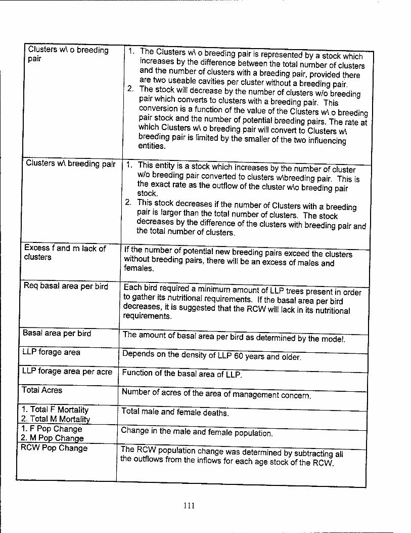
Clusters w\ o breeding pair
Clusters w\ breeding pair
Excess f and m lack of clusters
Req basal area per bird
Basal area per bird
LLP forage area
LLP forage area per acre
Total Acres
1. Total F Mortality 2. Total M Mortality 1. FPop Change 2. M Pop Change RCW Pop Change
1. The Clusters w\ o breeding pair is represented by a stock which increases by the difference between the total number of clusters and the number of clusters with a breeding pair, provided there are two useable cavities per cluster without a breeding pair
2. The stock will decrease by the number of clusters w/o breeding pair which converts to clusters with a breeding pair This conversion is a function of the value of the Clusters w\ o breeding pair stock and the number of potential breeding pairs The rate at which Clusters w\ o breeding pair will convert to Clusters w\ breeding pair is limited by the smaller of the two influencinq entities. a
1- This entity is a stock which increases by the number of cluster— w/o breeding pair converted to clusters w\breeding pair This is the exact rate as the outflow of the cluster w\o breedinq pair stock. a K
2. This stock decreases if the number of Clusters with a breeding pair is larger than the total number of clusters The stock decreases by the difference of the clusters with breeding pair and the total number of clusters.
If the number of potential new breeding pairs exceed the clusters" without breeding pairs, there will be an excess of males and females.
Each bird required a minimum amount of LLP trees present in order to gather its nutritional requirements. If the basal area per bird decreases, it is suggested that the RCW will lack in its nutritional requirements.
The amount of basal area per bird as determined by the model.
Depends on the density of LLP 60 years and older.
Function of the basal area of LLP.
Number of acres of the area of management concern.
Total male and female deaths.
Change in the male and female population.
The RCW population change was determined by subtracting all the outflows from the inflows for each age stock of the RCW.
Ill
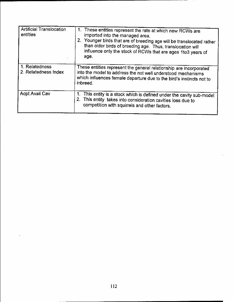
Artificial Translocation entities
1. Relatedness 2. Relatedness Index
Acpt Avail Cav
1. These entities represent the rate at which new RCWs are imported into the managed area.
2. Younger birds that are of breeding age will be translocated rather than older birds of breeding age. Thus, translocation will influence only the stock of RCWs that are ages 1to3 years of age.
These entities represent the general relationship are incorporated into the model to address the not well understood mechanisms which influences female departure due to the bird's instincts not to inbreed.
1. This entity is a stock which is defined under the cavity sub-model. 2. This entity takes into consideration cavities loss due to
competition with squirrels and other factors.
112

Appendix B
The following pages contain the structure of the system dynamics model utilized for the project. The model is divided into three sectors: tree, RCW, and cavity. See Chapter 4 for general comments regarding the model and Appendix A for assumptions made in constructing the model.
113

c©0 Tree
LLP 1to30 ideal stem dens Area
LLP time bet thinning
LLP germ
TO Shading
TO stem density LLP density
LLP 30 to 60
LLP 30to60 Ips beetle infest f "\ Ntrl Mort 30to60
1" Nat Mort Multiplier
114
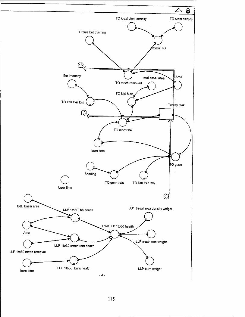
total basal area
"Ogerm
burn time TO germ rate TO Dth Per Bm
o LLP basal area density weight
LLP mech rem weight
LLP 1to30 mech removal
burn time LLP 1to30 burn health LLP burn weight
115
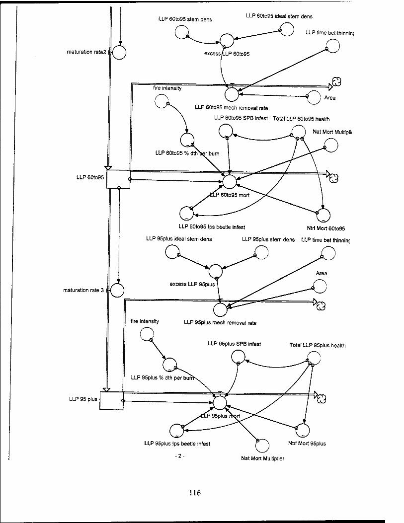
maturation rate2 I
LLP 60to95 stem dens LLP 60to95 ideal stem dens
o LLP time bet thinninc
LLP 60to95
\Z.
fire intensity
LLP 60to95 mech removal rate
LLP 60to95 SPB infest Total LLP 60to95 health
Nat Mort Multiplii
LLP 60to95 % dthlser bum
LLP 60to95 Ips beetle infest Ntrl Mort 60to95
LLP 95plus ideal stem dens LLP 95plus stem dens LLP time bet thinnin<
maturation rate 3 I
LLP 95 plus
Total LLP 95plus health
LLP 95plus Ips beetle infest
-2-
Ntrl Mort 95plus
Nat Mort Multiplier
116
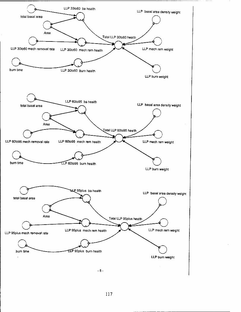
LLP 30to60 ba health LLP basal area density weight
burn time LLP30to60 burn health
LLP burn weight
LLP basal area density weight
LLP 60to95 mech removal rate LLP 60to95 mech rem health
burn time
LLP mech rem weight
LLP bum weight
total basal area
LLP 95plus mech removal rate
o burn time
LLP basal area density weight
Jotal LLP 95plus health _
LLP 95plus mech rem health Xv—/"*,sv LLP mecn rem weight
LLP bum weight
-5-
117
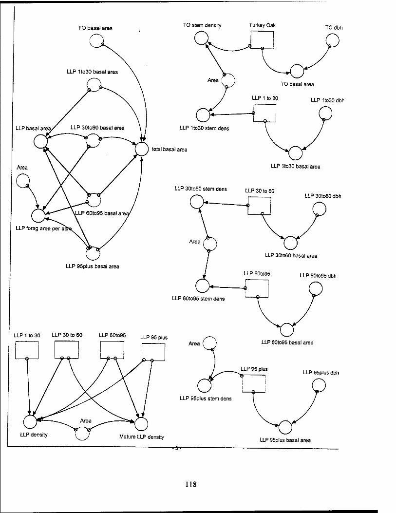
TO basal area TO stem density Turkey Oak TOdbh
total basal area
LLP1to30dbh
LLP1to30 stem dens
LLP1to30 basal area
LLP 30to60 stem dens n_p 3010 60
LLP 30to60 dbh
LLP 95plus basal area
LLP 60to95 dbh
LLP 60to95 stem dens
LLP 1 to 30 LLP 30 to 60 LLP 60to95 LLp 95 plus
Mature LLP density
Area
LLP 95plus dbh
LLP 95plus stem dens
LLP 95plus basal area
118
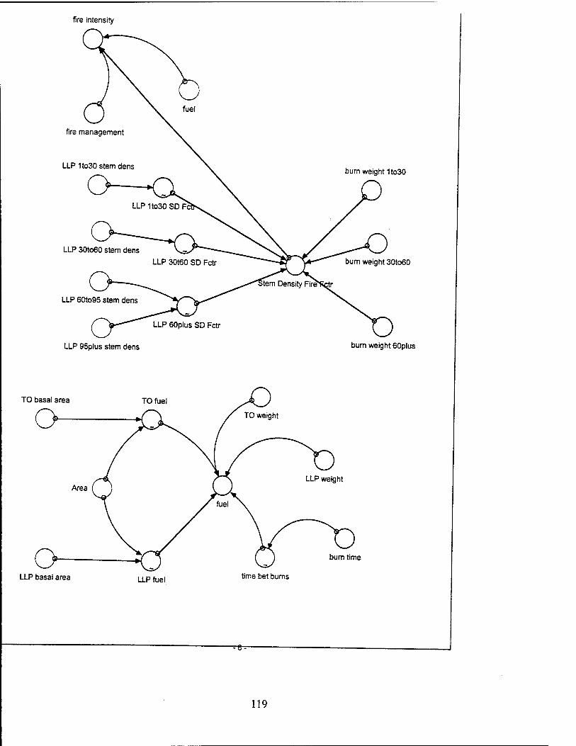
fire intensity
fire management
LLP1to30 stem dens
LLP 30to60 stem dens
LLP 60to95 stem dens
LLP 95plus stem dens
burn weight 1to30
LLP 30t60 SD Fctr ST V bum weight 30to60
Stem Density Fire^Rqtr
bum weight 60plus
TO basal area
LLP basal area
time
LLP fuel time bet bums
119
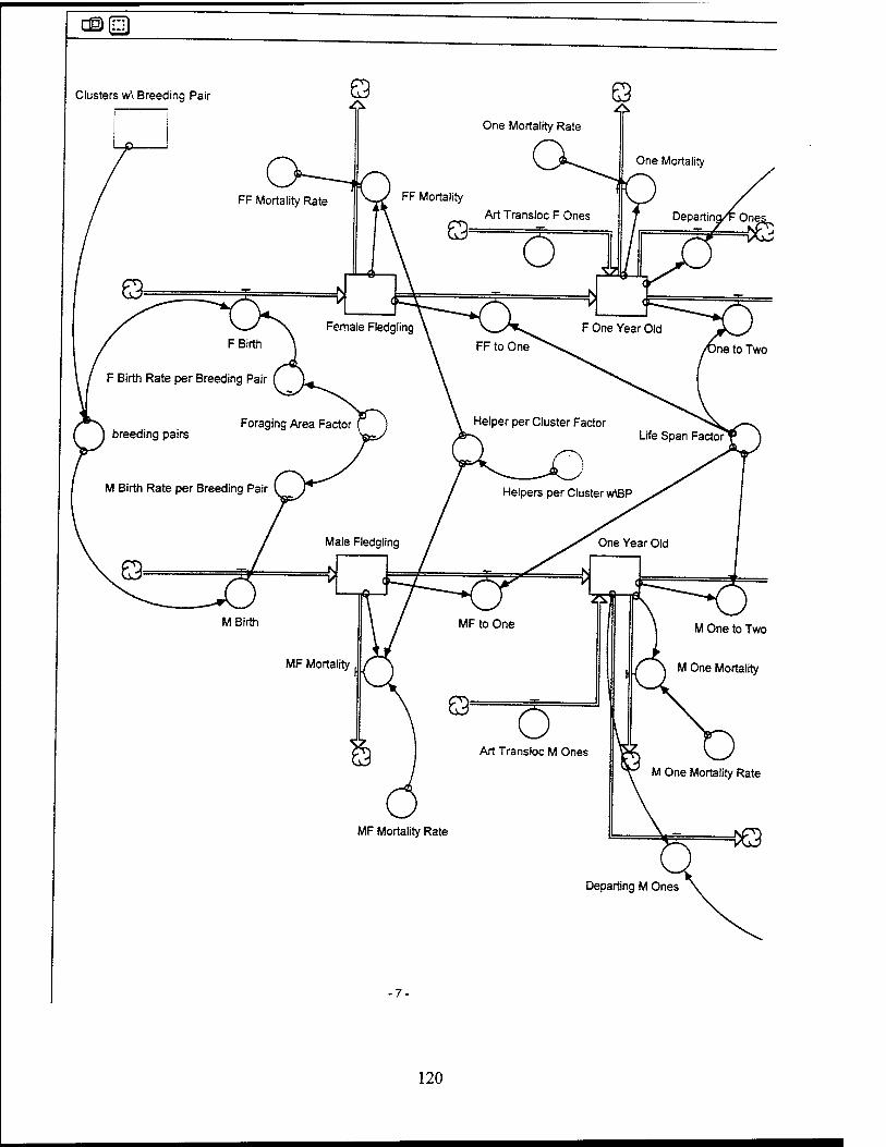
120
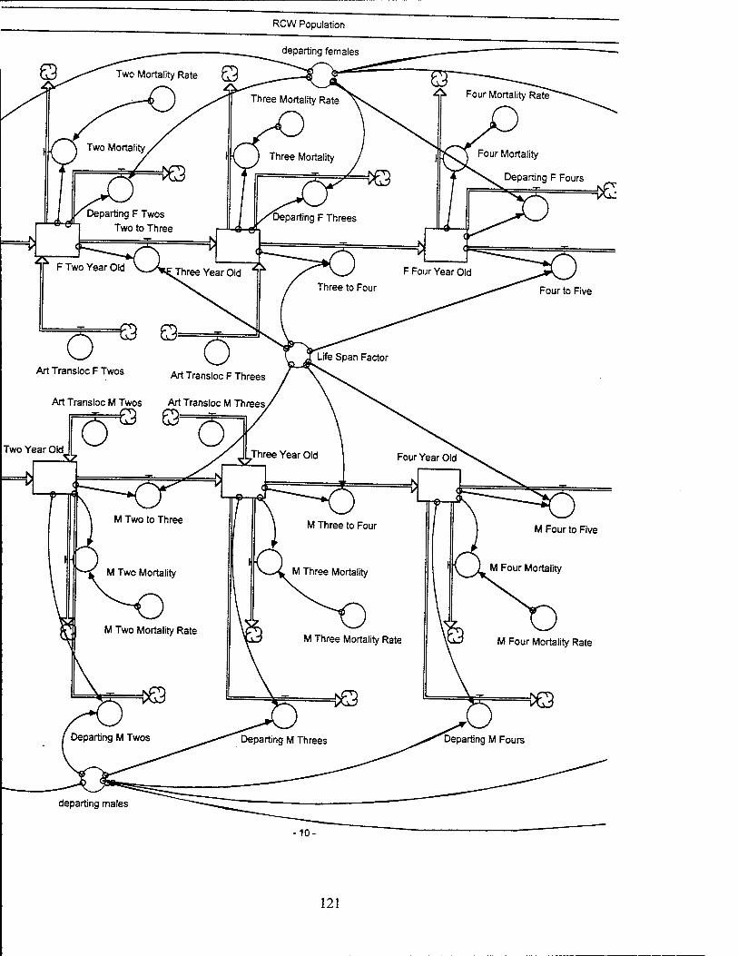
RCW Population
departing males
10-
121
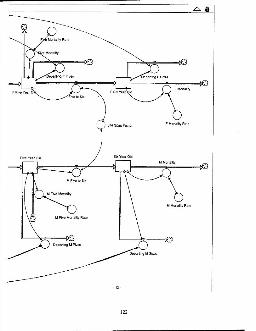
z^ 8
Departing M Sixes
13-
122
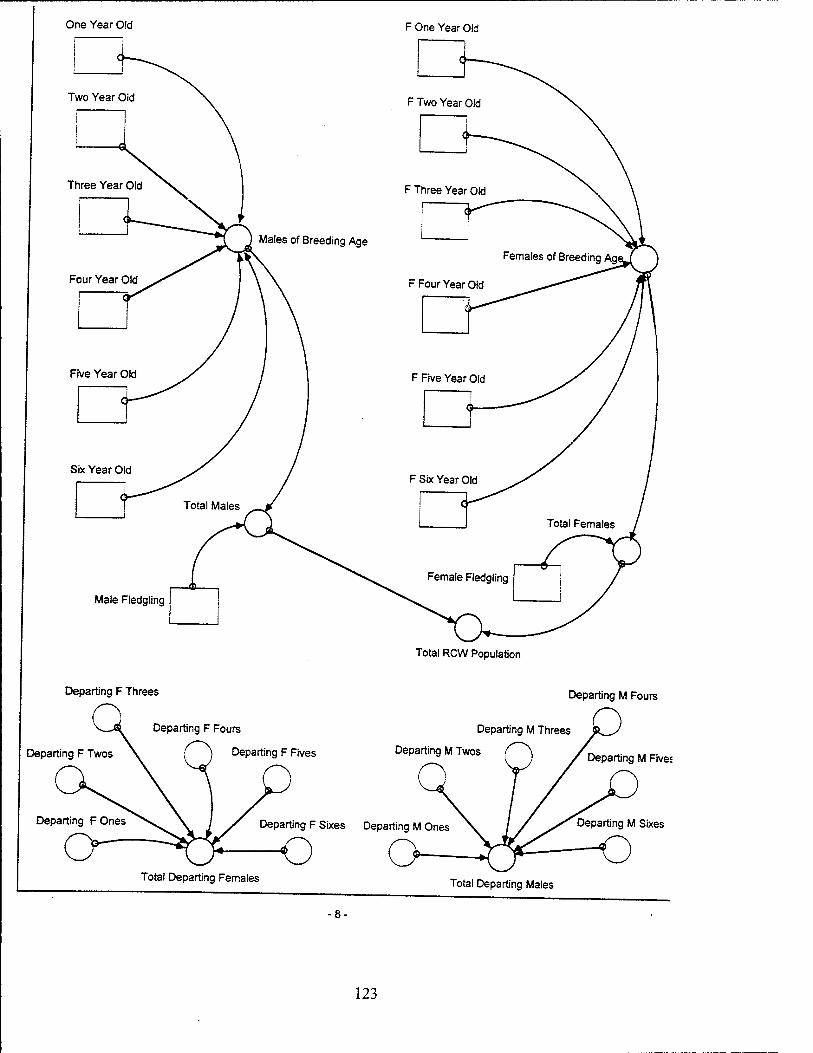
One Year Old
Two Year
F One Year Old
Three Year
Male Fledgling
Total RCW Population
Departing F Threes
Departing F Fours
Departing F Twos \ ( ) Departing F Fives
Departing M Fours
Departing M Threes
Departing M Twos Departing M Fives
Departing FOnes Departing F Sixes Departing M Ones
-—o o- Total Departing Females Total Departing Males
-8-
123
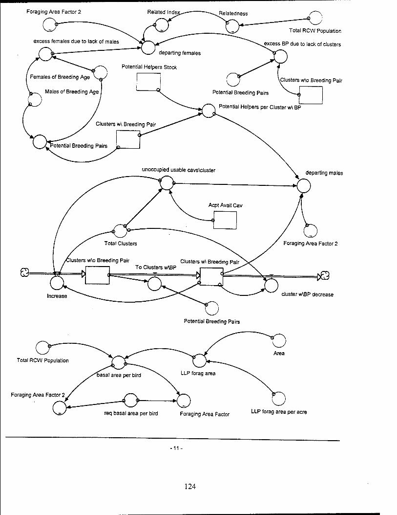
Foraging Area Factor 2 Related Inde:
Total RCW Population
excess BP due to lack of clusters
Clusters w\o Breeding Pair
Potential Breeding Pairs
Total RCW Population
Foraging Area Factor 2
departing males
Foraging Area Factor 2
H>Q cluster w\BP decrease
req basal area per bird Foraging Area Factor LLP forag area per acre
-11
124
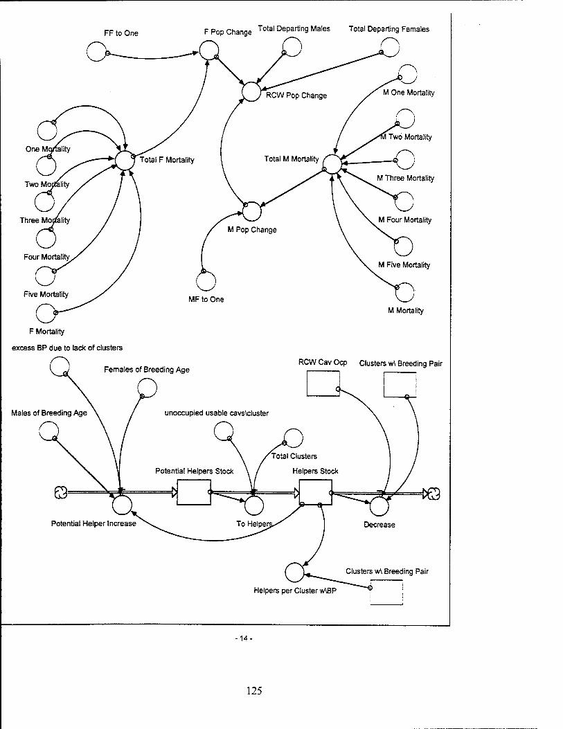
FF to One F Pop Change Total DePartin9 Males Total Departing Females
One Mortality
Two Mortality
Three Mortality
Four Mortality
Five Mortality
F Mortality
excess BP due to lack of clusters
M One Mortality
Two Mortality
M Three Mortality
M Four Mortality
M Five Mortality
M Mortality
Females of Breeding Age RCW Cav Ocp Clusters w\ Breeding Pair
Males of Breeding Age
Potential Helper Increase
Helpers per Cluster w\BP
-14-
125
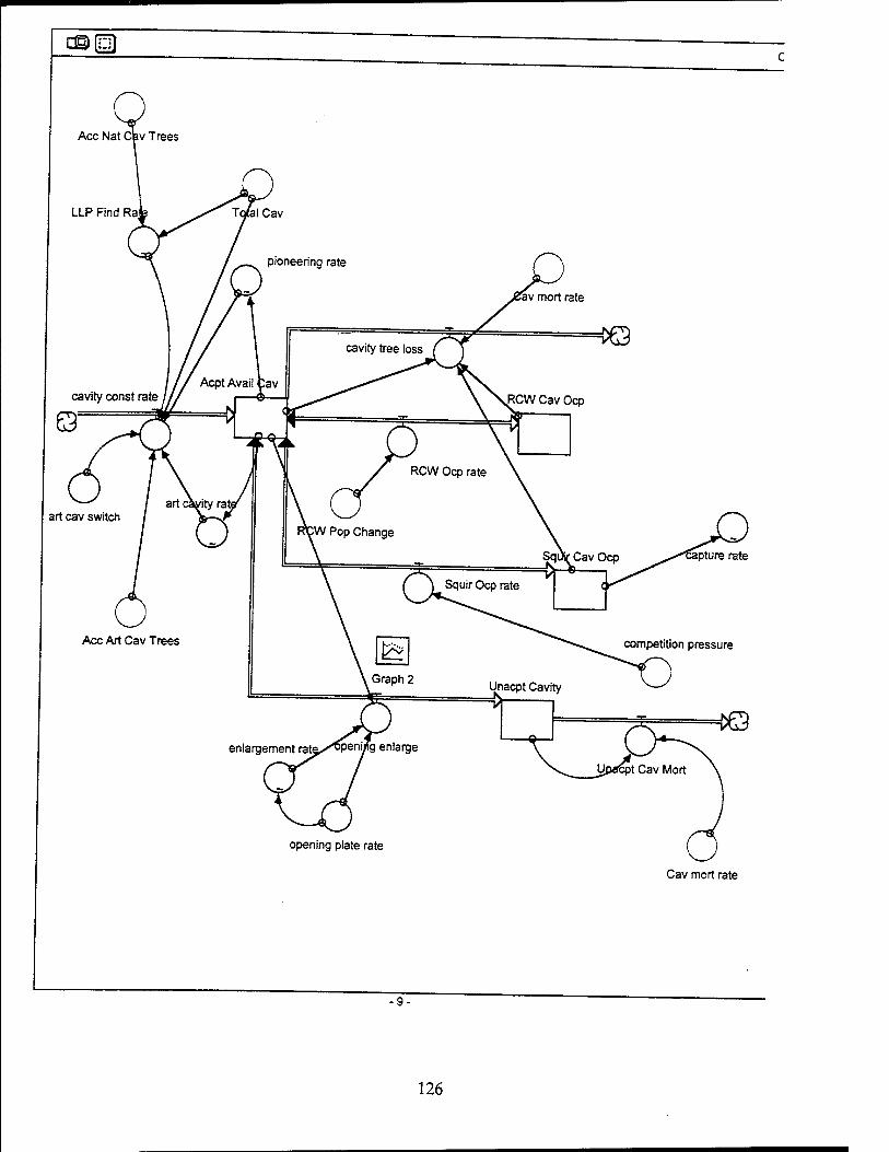
opening plate rate
Cav mort rate
-9-
126
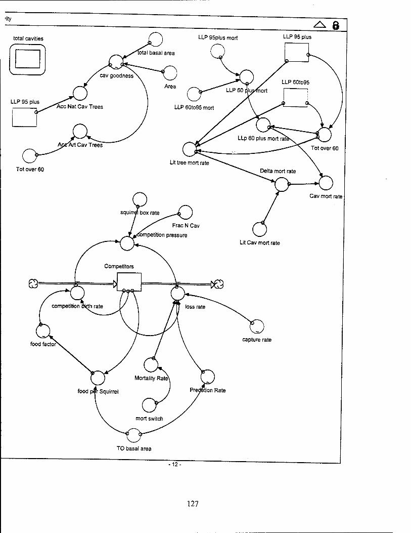
12-
127

Appendix C
The following pages contain the equations and values employed in the system dynamics model utilized for the project. See Chapter 4 for general comments regarding the model and Appendix A for assumptions made in constructing the model.
128
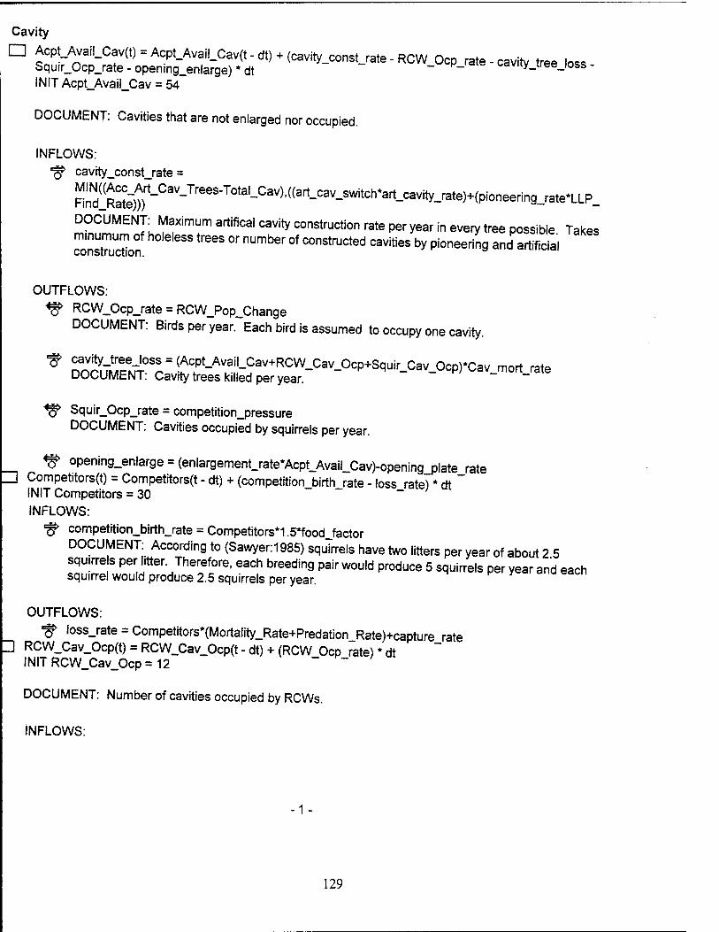
Cavity
□ Acpt_AvaiLCav(t) = Acpt_Avai!_Cav(t-dt) + (cavity_const_rate-RCW Ocp rate-cavity tree loss Squir_Ocp_rate - opening_enlarge) * dt " caviiy_iree_ioss- INIT Acpt_Avail_Cav = 54
DOCUMENT: Cavities that are not enlarged nor occupied.
INFLOWS: "§> cavity_const_rate =
FIII^R^
DOCUMENT: Maximum artifical cavity construction rate per year in every tree possible Takes
ZsZ2°n h0le,eSS treeS °r nUmber °f C°nStrUCted CaV"ieS by Pione^g andSi
OUTFLOWS: <^> RCW_Ocp_rate = RCW_Pop_Change
DOCUMENT: Birds per year. Each bird is assumed to occupy one cavity.
* noSf^ptT^r !fcpt-Avail-Cav+RCW-Cav_Ocp+Squir_Cav_Ocp)*Cav mort rate DOCUMENT: Cavity trees killed per year. ~ _
^ Squir_Ocp_rate = competition_pressure DOCUMENT: Cavities occupied by squirrels per year.
<§> opening_enlarge = (enlargement_rate*Acpt_Avail_Cav)-opening_plate_rate Z3 Competitors(t) = Competitors(t-dt) +(competition birth rate-loss rate)*dt
INIT Competitors = 30 ~ ~ INFLOWS:
■§> competition_birth_rate = Competitors*1.5*food_factor DOCUMENT: According to (Sawyer:1985) squirrels have two litters per year of about 2 5 squ.rre s per litter Therefore, each breeding pair would produce 5 squirrels per year and each squirrel would produce 2.5 squirrels per year.
OUTFLOWS:
"# loss_rate = Competitors*(Mortality_Rate+Predation_Rate)+capture rate H RCW_Cav_Ocp(t) = RCW_Cav_Ocp(t - dt) + (RCW Ocp rate) * dt
INITRCW_Cav_Ocp=12 "
DOCUMENT: Number of cavities occupied by RCWs.
INFLOWS:
-1
129
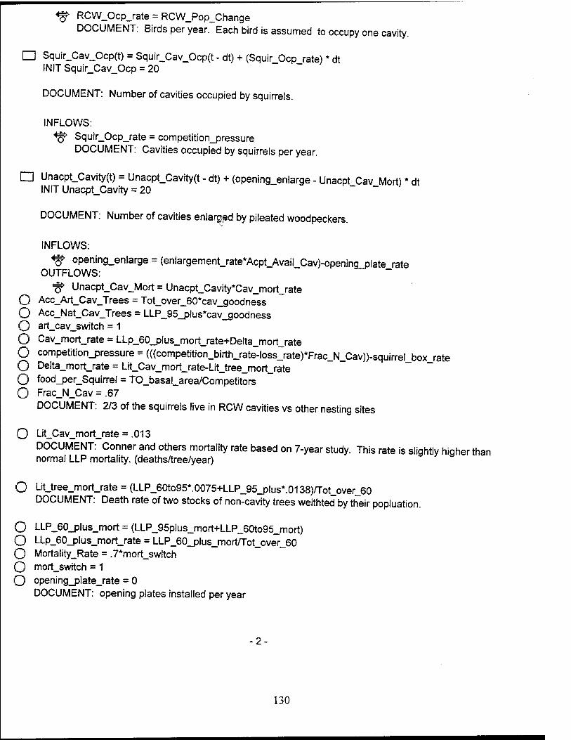
«g> RCW_Ocp_rate = RCW_Pop_Change DOCUMENT: Birds per year. Each bird is assumed to occupy one cavity.
□ Squir_Cav_Ocp(t) = Squir_Cav_Ocp(t - dt) + (Squir_Ocp_rate) * dt INIT Squir_Cav_Ocp = 20
DOCUMENT: Number of cavities occupied by squirrels.
INFLOWS: *§> Squir_Ocp_rate = competition_pressure
DOCUMENT: Cavities occupied by squirrels per year.
□ Unacpt_Cavity(t) = Unacpt_Cavity(t - dt) + (opening_enlarge - Unacpt Cav Mort) * dt INIT Unacpt_Cavity = 20 ~ ~
DOCUMENT: Number of cavities enlarged by pileated woodpeckers.
INFLOWS:
«^ opening_enlarge = (enlargement_rate*Acpt_Avail_Cav)-opening_plate rate OUTFLOWS:
^ Unacpt_Cav_Mort = Unacpt_Cavity*Cav_mort_rate O Acc_Art_Cav_Trees = Tot_over_60*cav_goodness O Acc_Nat_Cav_Trees = LLP_95_plus*cav_goodness O art_cav_switch = 1
O Cav_mort_rate = LLp_60_plus_mort_rate+Delta_mort_rate
O competition_pressure = (((competition_birth_rate-loss_rate)*Frac_N_Cav))-squirrel_box_rate O Delta_mort_rate = Lit_Cav_mort_rate-Lit_tree_mort_rate O food_per_Squirrel = TO_basal_area/Competitors O Frac_N_Cav = .67
DOCUMENT: 2/3 of the squirrels live in RCW cavities vs other nesting sites
O Lit_Cav_mort_rate = .013
DOCUMENT: Conner and others mortality rate based on 7-year study. This rate is slightly higher than normal LLP mortality, (deaths/tree/year)
O Lit_tree_mort_rate = (LLP_60to95*.0075+LLP_95_plus*.0138)/Tot_over_60 DOCUMENT: Death rate of two stocks of non-cavity trees weithted by their popluation.
O LLP_60_plus_mort = (LLP_95plus_mort+LLP_60to95_mort) O LLp_60_plus_mort_rate = LLP_60_plus_mort/Tot_over_60 O Mortality_Rate = .7*mort_switch O mort_switch = 1 O opening_plate_rate = 0
DOCUMENT: opening plates installed per year
-2
130
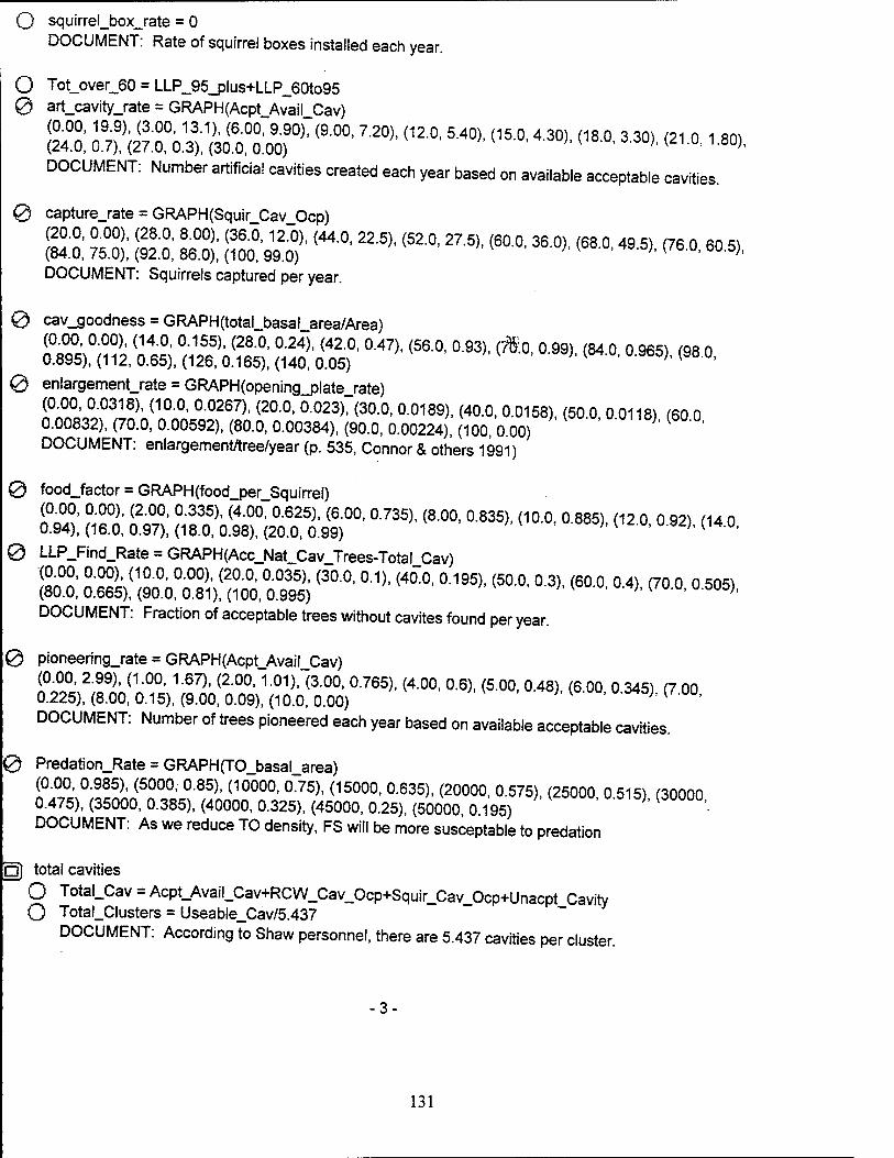
O squirrel_box_rate = 0 DOCUMENT: Rate of squirrel boxes installed each year.
O Tot_over_60 = LLP_95_plus+LLP_60to95 0 art_cavity_rate = GRAPH(Acpt Avail_Cav)
!24°o0; ^'^^:^^00'720)'(120' 5-40)' (15-°- 4-30)-(18-0' 3-30>- ™ ^ DOCUMENT: Number artificial cavities created each year based on available acceptable cavities.
0 capture_rate = GRAPH(Squir CavJDcp)
££ k°3: ££ £$ SÄ(440' 22-5)'(520'27* ^ 36°>< ^ «* ™ «^ DOCUMENT: Squirrels captured per year.
0 cav_goodness = GRAPH(total_basal_area/Area) (0.00, 0.00), (14.0, 0.155), (28.0, 0.24), (42.0, 0.47), (56.0, 0.93), (Mo, 0.99) (84 0 0 965) (98 0 0.895), (112,0.65), (126,0.165), (140,0.05) '"{ ' h (98°'
0 enlargement_rate = GRAPH(opening_plate_rate) (0.00, 0.0318), (10.0, 0.0267), (20.0, 0.023), (30.0, 0.0189), (40.0, 0.0158), (50 0 0 0118) (60 0 0.00832), (70.0, 0.00592), (80.0, 0.00384), (90.0, 0.00224), (100, 0 00) DOCUMENT: enlargement/tree/year (p. 535, Connor & others 1991)
0 food_factor = GRAPH(food_per Squirrel) (0 00, 0.00), (2.00, 0.335), (4.0o7o.625), (6.00, 0.735), (8.00, 0.835), (10.0. 0.885) (12 0 0 92) (14 0 0.94), (16.0,0.97), (18.0,0.98), (20.0,0.99) h { ' h ( °'
0 LLP_Find_Rate = GRAPH(Acc Nat Cav_Trees-Total_Cav)
££ SÄ!Z^Ä^i(3"00' °'u <40"a °'195)'(50a a3)'<6M'04)'(700' °'505>' DOCUMENT: Fraction of acceptable trees without cavites found per year.
0 pioneering_rate = GRAPH(Acpt_Avail_Cav) {^2tV\°0, 167)' (2°0, 101)' (300' 0765)- (400' °'6)' (50°. 0.48), (6.00, 0.345) (7 00 0.225), (8.00, 0.15), (9.00, 0.09), (10.0, 0.00) h K ' DOCUMENT: Number of trees pioneered each year based on available acceptable cavities.
0 Predation_Rate = GRAPH(TO_basal_area) (0.00, 0.985), (5000, 0.85), (10000, 0.75), (15000, 0.635), (20000, 0.575), (25000, 0 515) (30000 0.475), (35000, 0.385), (40000, 0.325), (45000, 0.25), (50000, 0.195) DOCUMENT: As we reduce TO density, FS will be more susceptable to predation
□) total cavities
O Total.Cav = Acpt_Avail_Cav+RCW_Cav_Ocp+Squir_Cav_Ocp+Unacpt_Cavity O Total_Clusters = Useable_Cav/5.437
DOCUMENT: According to Shaw personnel, there are 5.437 cavities per cluster
131
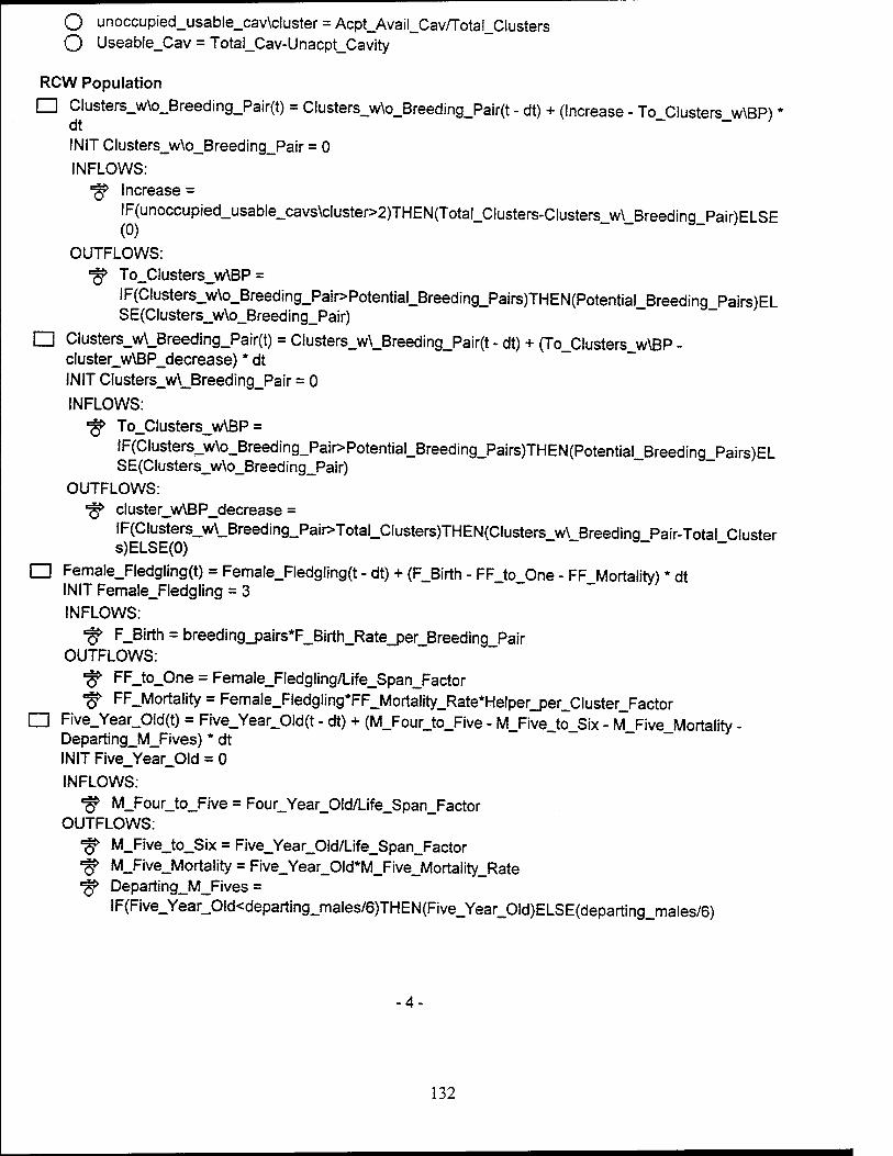
O unoccupied_usabie_cav\ciuster = Acpt_Avail_Cav/Total_Clusters O Useable_Cav = Totai_Cav-Unacpt_Cavity
RCW Population
□ Clusters_w\o_Breeding_Pair(t) = Clusters_w\o_Breeding_Pair(t - dt) + (Increase - To_Clusters_w\BP) * dt INIT C!usters_w\o_Breeding_Pair = 0 INFLOWS:
"g Increase =
IF(unoccupied_usable_cavs\cluster>2)THEN(Total_Clusters-Clusters_w\_Breeding_Pair)ELSE
OUTFLOWS: °Q> To_Clusters_w\BP =
IF(Clusters_w\o_Breeding_Pair>Potential_Breeding_Pairs)THEN(Potential_Breeding_Pairs)EL SE(Clusters_w\o_Breeding_Pair)
□ Clusters_w\_Breeding_Pair(t) = Clusters_w\_Breeding_Pair(t - dt) + (To_Clusters_w\BP - cluster_w\BP_decrease) * dt INIT Clusters_w\_Breeding_Pair = 0
INFLOWS: •§■ To_Clusters_w\BP =
IF(Clusters_w\o_Breeding_Pair>Potential_Breeding_Pairs)THEN(Potential_Breeding_Pairs)EL SE(Clusters_w\o_Breeding_Pair)
OUTFLOWS: ■§> cluster_w\BP_decrease =
IF(Clusters_w\_Breeding_Pair>Total_Clusters)THEN(Clusters w\ Breeding Pair-Total Cluster s)ELSE(O) ~
□ Female_Fledgling(t) = Female_Fledgling(t - dt) + (F_Birth - FF_to_One - FF_Mortality) * dt INIT Female_Fledgling = 3 INFLOWS:
-^ F_Birth = breeding_pairs*F_Birth_Rate_per_Breeding_Pair OUTFLOWS:
"gf FF_to_One = Female_Fledgling/Life_Span_Factor
•%> FF_Mortality = Female_Fledgling*FF_Mortality_Rate*Helper_per_Cluster_Factor □ Five_Year_Old(t) = Five_Year_Old(t - dt) + (M_Four_to_Five - M_Five_to_Six - M_Five_Mortality -
Departing_M_Fives) * dt INIT Five_Year_Old = 0
INFLOWS: ■^ M_Four_to_Five = Four_Year_Old/Life_Span_Factor
OUTFLOWS: ■§> M_Five_to_Six = Five_Year_Old/Life_Span_Factor ■§> M_Five_Mortality = Five_Year_Old*M_Five_Mortality_Rate *§> Departing_M_Fives =
IF(Five_Year_Old<departing_males/6)THEN(Five_Year_Old)ELSE(departing_males/6)
-4-
132
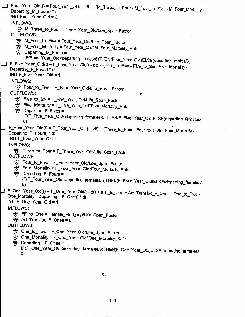
° DSJTF^^rear-°ld(t ■dt> + <M-Th--'°-F- - M-PouMcFive - M.Four.Mor«a,ity
INIT Four_Year_Old = 0
INFLOWS:
■f> M_Three_to_Four = Three_Year_Old/Life_Span Factor OUTFLOWS:
■^ M_Four_to_Five = Four_Year_Old/Life_Span_Factor ■§> M_Four_Mortality = Four_Year_Old*M_Four_Mortality_Rate ^ Departing_M_Fours =
IF(Fo"r-Year_Old<departing_males/6)THEN(Four_Year_Old)ELSE(departing ma!es/6) □ F_F.ve_Year Old(t) = F Five_Year_Oid(t-dt)MFour_to_Five-FiveJo Six-Five Mortality-
Departing_F_Fives) * dt - w,ia"iy
INIT F_Five_Year_Old = 1
INFLOWS:
■^ Four_to_Five = F_Four_Year_Old/Life_Span Factor OUTFLOWS: 8
«^ Five_to_Six = F_Five_Year_Old/Life_Span_Factor ^ Five_Mortality = F_Five_Year_Old*Five_Mortality_Rate ■§> Departing_F_Fives =
F(F_Five_Year_Old<departing_females/6)THEN(F_Five_Year_Old)ELSE(departing_females/
] DS^S r^-^-01^ -*> + (Three.to.Four - Four_to_Five - Four_Morta.ity -
INIT F_Four_Year_Old = 1 INFLOWS:
f? Three_to_Four = F_Three_Year_Old/Life_Span Factor OUTFLOWS:
■§> Four_to_Five = F_Four_Year_Old/Life_Span_Factor ^ Four_Mortality = F_Four_Year_Old*Four_Mortality_Rate ■^ Departing_F_Fours =
F(F_Four_Year_Old<departing_females/6)THEN(F_Four_Year_Old)ELSE(departing_females/
' ^r^!"01^ F Ones-One to Two- One_Mortality - Departing_F_Ones) * dt ~ ~ - INIT F_One_Year_Old = 1 INFLOWS:
"& FF_to_One = Female_Fledgling/Life_Span_Factor *§■ Art_Transloc_F_Ones = 0
OUTFLOWS:
■^ One_to_Two = F_One_Year_Old/Life_Span_Factor ^ One_Mortality = F_One_Year_Old*One_Mortality_Rate ■^ Departing F_Ones =
F(F_One_Year_Old<departing_females/6)THEN(F_One_Year_Old)ELSE(departing_females/
1^ ^
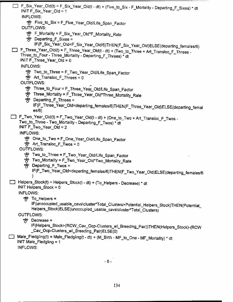
□ F_Six_Year_Old(t) = F_Six_Year_Old(t- dt) + (FiveJo.Six - FJ/lortality - Departing F Sixes) * dt I NIT F_Six_Year_Oid = 1 INFLOWS:
■§> Five_to_Six = F_Five_Year_Old/Life_Span_Factor OUTFLOWS:
■^ F_Mortality = F_Six_Year_Old*F_Mortality_Rate •f? Departing_F_Sixes =
IF(F_Six_Year_0ld<F_Six_Year_0ld/6)THEN(F_Six_Year_0ld)ELSE(departing_females/6) □ F_Three_Year_Old(t) = F_Three_Year_Old(t - dt) + (Two_to_Three + Art_Transloc_F_Threes -
Three_to_Four - Three_Mortality - Departing_F_Threes) * dt INIT F_Three_Year_Old = 0 INFLOWS:
■^ Two_to_Three = F_Two_Year_Old/Life_Span_Factor *$> Art_Transloc_F_Threes = 0
OUTFLOWS:
■^ Three_to_Four = F_Three_Yea^Old/Life_Span_Factor ■§> Three_Mortality = F_Three_Year_Old*Three_Mortality_Rate "§?> Departing_F_Threes =
IF(F_Three_Year_Old<departing_females/6)THEN(F_Three_Year_Old)ELSE(departing femal es/6)
□ F_Two_Year_Old(t) = F_Two_Year_Old(t - dt) + (One_to_Two + Art_Transloc_F_Twos - Two_to_Three - Two_Mortality - Departing_F_Twos) * dt INIT F_Two_Year_Old = 2 INFLOWS:
■^ One_to_Two = F_One_Year_Old/Life_Span_Factor %> Art_Transloc_F_Twos = 0
OUTFLOWS:
■§> Two_to_Three = F_Two_Year_Old/Life_Span_Factor ■^ Two_Mortality = F_Two_Year_Old*Two_Mortality_Rate ^ Departing_F_Twos =
IF(F_Two_Year_Old<departing_females/6)THEN(F_Two_Year_Old)ELSE(departing_females/6
□ He!pers_Stock(t) = Helpers_Stock(t - dt) + (To_Helpers - Decrease) * dt INIT Helpers_Stock = 0 INFLOWS: ^ To_Helpers =
IF(unoccupied_usable_cavs\cluster*Total_Clusters>Potential_Helpers_Stock)THEN(Potential_ Helpers_Stock)ELSE(unoccupied_usable_cavs\cluster*Total_Clusters)
OUTFLOWS: ^ Decrease =
IF(Helpers_Stock>(RCW_Cav_Ocp-Clusters_w\_Breeding_Pair))THEN(Helpers_Stock)-(RCW _Cav_Ocp-Clusters_w\_Breeding_Pair)ELSE(0)
□ Male_Fledgling(t) = Male_Fledgling(t - dt) + (M_Birth - MFJo One - MF Mortality) * dt INIT Male_Fledgling = 1 " INFLOWS:
-6-
134
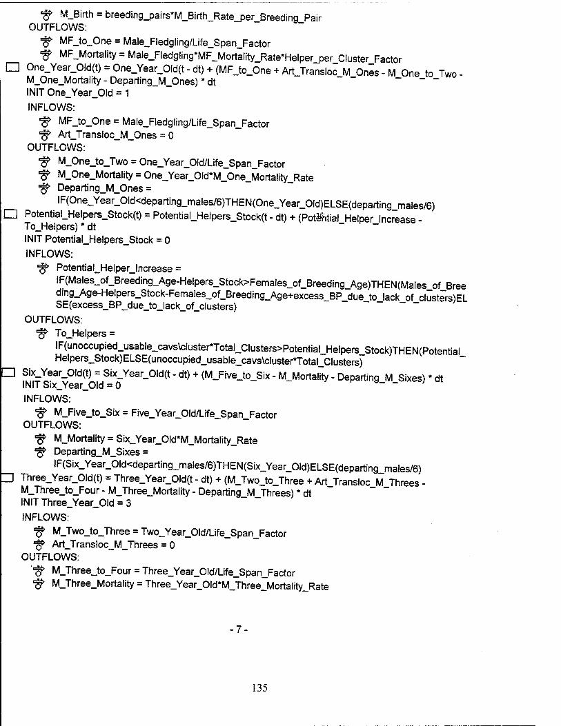
■§► M_Birth = breeding_pairs*M_Birth_Rate_per_Breeding Pair OUTFLOWS:
■§► MF_to_One = Male_Fledgling/Life_Span_Factor
^> MF_Mortality = Male_Fledgling*MF_Mortality_Rate*Helper_per_Cluster_Factor □ One_Year_Old(t) = One_Year_Old(t-dt) + (MF_to_One + Art_Transloc_M Ones-M One to Two-
M_One_Mortality - Departing_M_Ones) * dt ~ ~ ~ INIT One_Year_Old = 1
INFLOWS:
•$ MF_to_One = Male_Fledgling/Life_Span_Factor ■§> Art_Transloc_M_Ones = 0
OUTFLOWS:
■§> M_One_to_Two = One_Year_Old/Life_Span_Factor •# M_One_Mortality = One_Year_Old*M_One_Mortality_Rate *§■ Departing_M_Ones =
IF(0ne_Year_0ld<departing_males/6)THEN(0ne_Year_0ld)ELSE(departing_males/6) □ Potential_Helpers_Stock(t) = Potentia!_Helpers_Stock(t - dt) + (Potential Helper Increase -
To_Helpers) * dt INIT Potential_Helpers_Stock = 0 INFLOWS:
^ PotentialJHelperJncrease =
IF(Males_of_Breeding_Age-Helpers_Stock>Females_of_Breeding_Age)THEN(Males_of_Bree ding_Age-Helpers_Stock-Females_of_Breeding_Age+excess_BP_due to lack of clusters)EL SE(excess_BP_due_to_lack_of_clusters) ~
OUTFLOWS: "§> To_Helpers =
IF(unoccupied_usable_cavs\cluster*Total_Clusters>Potential_Helpers_Stock)THEN(Potential Helpers_Stock)ELSE(unoccupied_usable_cavs\cluster*Total_Clusters)
□ Six_Year_Old(t) = Six_Year_Old(t-dt) + (M_Five_to_Six-M_Mortality- Departing M Sixes) *dt INIT Six_Year_Old = 0 ~ INFLOWS:
■#• M_Five_to_Six = Five_Year_Old/Life_Span_Factor OUTFLOWS:
■gf M_Mortality = Six_Year_Old*M_Mortality_Rate ^ Departing_M_Sixes =
IF(Six_Year_Old<departing_males/6)THEN(Six_Year_Old)ELSE(departing_males/6) ] Three_Year_Old(t) = Three_Year_Old(t - dt) + (M_Two_to_Three + Art_Transloc_M Threes -
M_Three_to_Four - M_Three_Mortality - Departing_M_Threes) * dt INIT Three_Year_Old = 3
INFLOWS:
"§> M_Two_to_Three = Two_Year_Old/Life_Span_Factor *§> Art_Transloc_M_Threes = 0
OUTFLOWS:
"^ M_Three_to_Four = Three_Year_Old/Life_Span_Factor *# M_Three_Mortality = Three_Year_Old*M_Three_Mortality_Rate
135
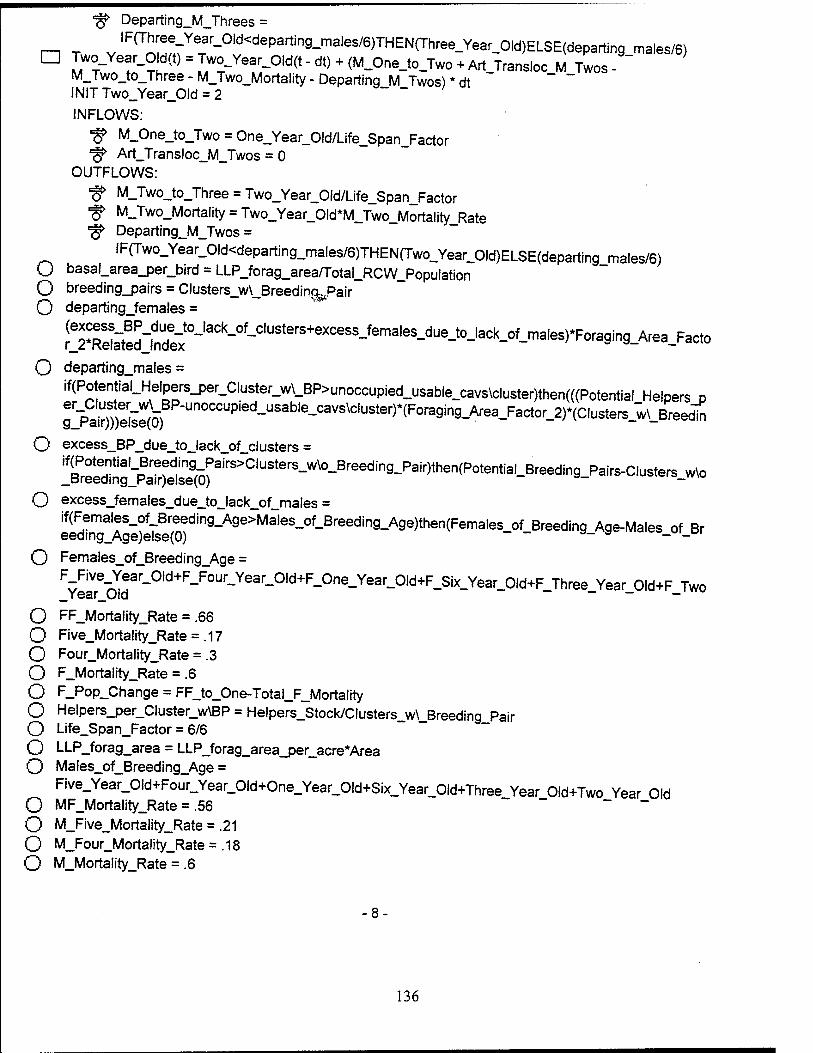
■ff Departing_M_Threes =
r-i T v ,F(T^Ü7Yerar-0id<departin9-ma,es/6)THEN(Three_Year_Old)ELSE(departing males/6) D MWT- ?-?^ (t) = LW°-Year-0ld(t" dt> + (M-One_to_Two + Art.Transloc M Twos -
M_Two_to_Three - M_Two_Mortality - Departing M Twos)* dt INIT Two_Year_Old = 2 INFLOWS:
^ M_One_to_Two = One_Year_Old/Life_Span_Factor ■ff Art_Transloc_M_Twos = 0
OUTFLOWS:
■§> M_Two_to_Three = Two_Year_Old/Life_Span_Factor ■§► M_Two_Mortality = Two_Year_Old*M_Two_Morta!ity_Rate ■ff Departing_M_Twos =
IFn"wo_Year_0!d<departing_males/6)THEN(Two_Year_Old)ELSE(departing_males/6) O basa!_area_per_bird = LLPJorag_area/Total_RCW_Population O breeding_pairs = Clusters_w\_Breedina^Pair O departing_females =
rl'Rel^fnd^ O departing_males =
if(Potential_Helpers^r_Cluster_w\_BP>unoccUpied_usable_cavs\cluster)then(((Potert^^ Helpers p
O excess_BP_due_to_lack_of_clusters =
Tre?d?ni3SS^ O excess_females_due_to_lack_of_males =
eTdin^A^ O Females_of_Breeding_Age =
V,Ve^!ar-Old+F-F0Ur-Year-Old+F-One-Year-Old+F-Six-Year-OW Three Year Old+F Two _Year_Old ~ — —
O FF_Mortality_Rate = .66 O Five_Mortality_Rate = .17 O Four_Mortality_Rate = .3 O F_MortaIity_Rate = .6 O F_Pop_Change = FF_to_One-Total_F_Mortality O Helpers_per_Cluster_w\BP = Helpers_Stock/Clusters_w\_Breeding_Pair O Life_Span_Factor = 6/6 O LLP_forag_area = LLP_forag_area_per_acre*Area O Males_of_Breeding_Age =
Five_Year_Old+Four_Year_Old+One_Year_Old+Six_Year_Old+Three_Year Old+Two Year Old O MF_Mortality_Rate = .56 O M_Five_Mortality_Rate = .21 O M_Four_Mortality_Rate = .18 O M_Morta!ity_Rate = .6
-8-
136
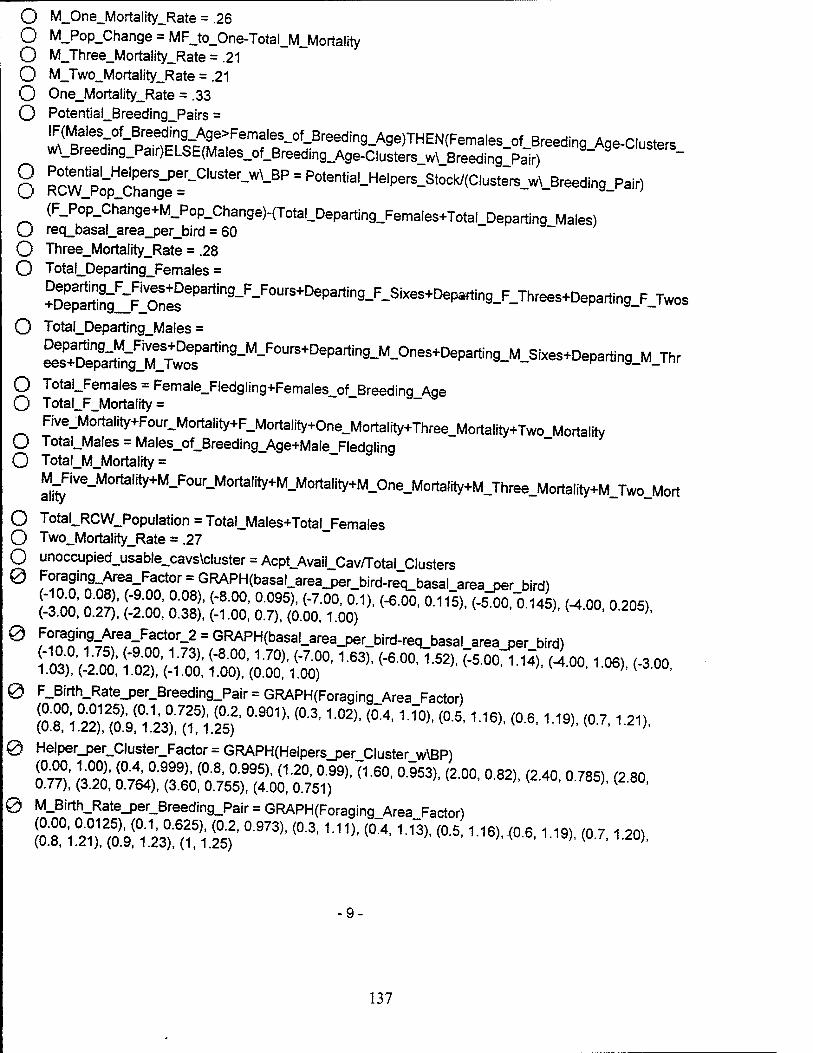
O M_One_Mortality_Rate = .26
O M_Pop_Change = MF_to_One-Total_M_Mortality O M_Three_Mortality_Rate = .21 O M_Two_Mortality_Rate = .21 O One_Mortality_Rate = .33 O Potential_Breeding_Pairs =
IF(Males oLBreeding Age>Females_of_Breeding_Age)THEN(Females of Breeding Age-Clusters w\_Breed.ng_Pa.r)ELSE(Males_of_Breeding_Age-Clusters_w\_Breeding:Pair) "
8 RcTpöpZ^e=~ClUS{eTJN-BP = P°tential-HelPers-Stock/(cl^ters_w\_Breeding_Pair)
(F_Pop_Change+M_Pop_Change)-(Total_Departing_Females+Total_Departing Males) O req_basa!_area_per_bird = 60 O Three_Mortality_Rate = .28 O Total_Departing_Females =
Sng^ O Total_Departing_Males =
O Total_Females = Female_Fledgling+Females of Breedinq Aqe O Total_F_Mortality = ~
Rve_Mortality+Four_Mortality+F_Mortality+One_Mortality+Three_Mortanty+Two_Mortality O Total_Males = Males_of_Breeding_Age+Male_Fledgling O Total_M_Mortality =
M_Five_Mortality+M_Four_Mortality+M_Mortality+M_One_Mortality^
O Total_RCW_Population = Total_Males+Total_Females O Two_Mortality_Rate = .27
O unoccupied_usable_cavs\cluster = Acpt_Avail Cav/Total_Clusters 0 T?nTn9nowV^ «».per bird)
tZ SS JSS S S£ Ä^1)'(-6'00'a,f5X ^"^ **"* 0 r^"?^,3/^0-2 = GRAPH(ba«Larea_per_bird-re<LbaSal area jar bird)
t1Ä ÄS: ESÄ3S* "*(-6'00' »*•r-5°°"* ^ -»• *** 0 F_Birtri_Rate_per_Breeding_Pair=GRAPH(Foraging_Area Factor)
MiSwÄ °'901>'(C'3'102)'^1 J0)'(05' 1'16)' (°'6' 1'19)'<C ?-1'21)' 0 Helper_per_Cluster_Factor= GRAPH(Helpers_per_Cluster_w\BP)
(0.00, 1.00), (0.4, 0.999), (0.8, 0.995), (1.20, 0.99), (1.60, 0.953), (2.00 0 82) (2 40 0 785) (2 80 0.77), (3.20,0.764), (3.60,0.755), (4.00,0.751) '' { ' }' (280,
0 M_Birth_Rate_per_Breeding_Pair = GRAPH(Foraging_Area Factor)
[ri02ufo)b!01.23°;6a)li°5)' °'973)' (°'3' 1'11X <A lf3)'(0'5' 116>' <°'6' "*■ w- '*»•
9-
137
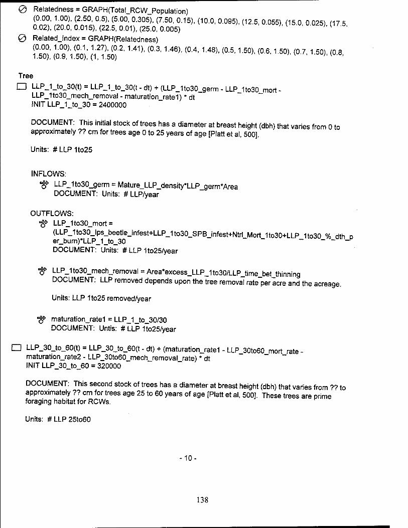
0 Reiatedness = GRAPH(Total_RCW_Population) (0.00, 1.00), (2.50, 0.5), (5.00, 0.305), (7.50, 0.15), (10.0, 0.095), (12.5, 0.055), (15 0 0 025) (17 5 0.02), (20.0, 0.015), (22.5, 0.01), (25.0, 0.005) ;' ( '
0 Relatedjndex = GRAPH(Relatedness)
ISO),' (10090)1(5°01); aJsS)2' 141)' (°-3, 146)' (04' 148)' (°-5' 1-50)- (0-6' 1"50^ <07' 1-5°)' «>■*>
Tree
□ LLP_1_to_30(t) = LLP_1_to_30(t - dt) + (LLP_1to30_germ - LLP_1to30_mort - LLP_1to30_mech_removal - maturation_rate1) * dt INIT LLP_1_to_30 = 2400000
DOCUMENT: This initial stock of trees has a diameter at breast height (dbh) that varies from 0 to approximately ?? cm for trees age 0 to 25 years of age [Platt et al, 500].
Units: # LLP 1to25
INFLOWS:
«^ LLP_1to30_germ = Mature_LLP_density*LLP_germ*Area DOCUMENT: Units: #LLP/year
OUTFLOWS: ■^ LLP_1to30_mort =
(LLP_1to30_lps_beetle_infest+LLP_1to30_SPB_infest+Ntrl_Mort 1to30+LLP 1to30 % dth D er_burn)*LLP_1_to_30 ~ ~ ~ DOCUMENT: Units: # LLP 1to25/year
■^ LLP_1to30_mech_removal = Area*excess_LLP_1to30/LLP_time_bet_thinning DOCUMENT: LLP removed depends upon the tree removal rate per acre and the acreage.
Units: LLP 1to25 removed/year
^ maturation_rate1 = LLP_1_to_30/30 DOCUMENT: Untis: # LLP 1to25/year
□ LLP_30_to_60(t) = LLP_30_to_60(t - dt) + (maturation_rate1 - LLP 30to60_mort rate - maturation_rate2 - LLP_30to60_mech_removal_rate) * dt INIT LLP_30_to_60 = 320000
DOCUMENT: This second stock of trees has a diameter at breast height (dbh) that varies from r? to
approximately ?? cm for trees age 25 to 60 years of age [Platt et al, 500]. These trees are prime foraging habitat for RCWs.
Units: # LLP 25to60
10-
138
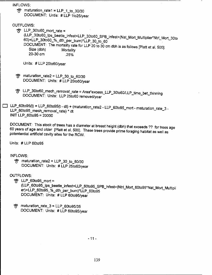
INFLOWS:
■§> maturation_rate1 = LLP_1_to_30/30 DOCUMENT: Untis: #LLP 1to25/year
OUTFLOWS: ■§> LLP_30to60_mort_rate =
60)+LLP_30to60_%_dth_per_burn)*LLP_30 to_60 ~ ~ D°o UM^uT; The m0rtality rate f0r LLP 20 *> 30 cm dbh is as allows [Platt et al 500V Size (dbh) Mortality
20-30 cm .25%
Units: # LLP 25to60/year
■^ maturation_rate2 = LLP_30_to_60/30 DOCUMENT: Units: # LLP 25to60/year
* ^°*f^ bet thinning DOCUMENT: Units: LLP 25to60 removed/year - - - a
0 ,L|-^°!^ rate 3- LLP_60to95_mech_removal_rate) * dt ~ INIT LLP_60to95 = 20000
DOCUMENT: This stock of trees has a diameter at breast height (dbh) that exceeds *r> for trees aae
nJZZSr\a9^Mel [P'attftal-50°3- These trees provide prime foraging habitat as well as potentential artificial cavity sites for the RCW.
Units: #LLP60to95
INFLOWS:
^ maturation_rate2 = LLP_30_to 60/30 DOCUMENT: Units: # LLP 25lo60/year
OUTFLOWS: •^ LLP_60to95_mort =
er)+LLP_60to95_%_dthjDer_burn)*LLP_60to95 DOCUMENT: Units: # LLP 60to95/year
°$> maturation_rate_3 = LLP_60to95/35 DOCUMENT: Units: # LLP 60to95/year
-11 -
139
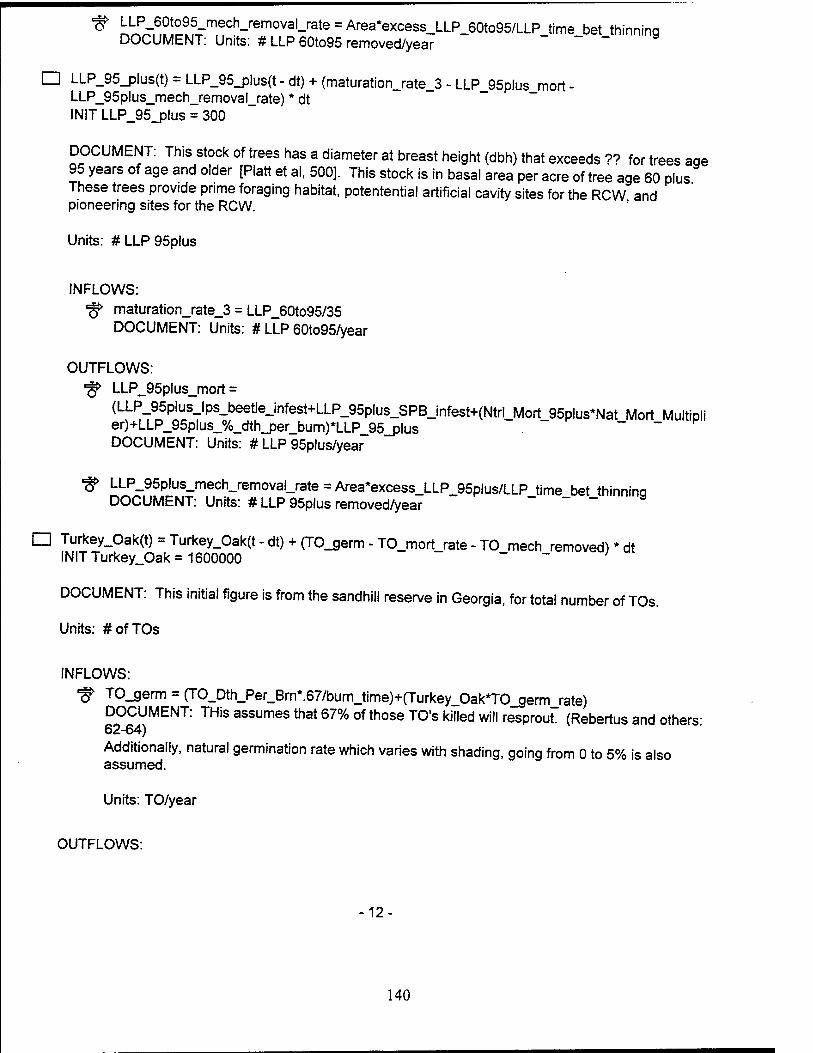
^ LLP_60to95_mech_removal_rate = Area*excess_LLP 60to95/LLP time bet thinnina DOCUMENT: Units: # LLP 60to95 removed/year " - - - nnm9
□ LLP_95_plus(t) = LLP_95_plus(t - dt) + (maturation_rate_3 - LLP_95plus_mort - LLP_95plus_mech_removal rate) * dt INIT LLP_95_plus = 300
DOCUMENT: This stock of trees has a diameter at breast height (dbh) that exceeds v> for trees aae 95 years of age and older [Platt et al, 500]. This stock is in basal area per acre of tree age 60 plus These trees provide prime foraging habitat, potentential artificial cavity sites for the RCW and pioneering sites for the RCW.
Units: #LLP95plus
INFLOWS:
■gr* maturation_rate_3 = LLP_60to95/35 DOCUMENT: Units: # LLP 60to95/year
OUTFLOWS: *§► LLP_95plus_mort =
(LLP_95plusJps_beetle_infest+LLP_95plus_SPB_infest+(Ntrl_Mort 95plus*Nat Mort Multipli er)+LLP_95plus_%_dth_per_burn)*LLP_95_plus ~ ~ DOCUMENT: Units: # LLP 95plus/year
■§> LLP_95plus_mech_removal_rate = Area*excess_LLP_95plus/LLP time bet thinnina DOCUMENT: Units: # LLP 95plus removed/year - - - a
□ Turkey_Oak(t) = Turkey_Oak(t - dt) + (TO_germ - TO_mort rate - TO mech removed) * dt INIT Turkey_Oak= 1600000 " " ;
DOCUMENT: This initial figure is from the sandhill reserve in Georgia, for total number of TOs.
Units: # of TOs
INFLOWS:
■f> TO_germ = (T0_Dth_Per_Bm*.67/bum_time)+(Turkey_0ak*T0_germ_rate) DOCUMENT: THis assumes that 67% of those TO's killed will resprout. (Rebertus and others- 62-64)
Additionally, natural germination rate which varies with shading, going from 0 to 5% is also assumed.
Units: TO/year
OUTFLOWS:
-12-
140
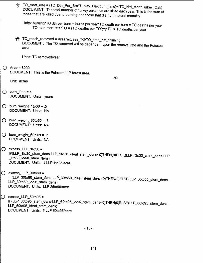
* HSTÄS8 = (TO-Dth-Per-Bm*TurkeV-0ak/burn_time)+(TO_NtrLMort*Turkey Oak) DOCUMENT: The total number of turkey oaks that are killed each year. This is the"sum of those that are killed due to burning and those that die from natural mortality.
Units: burning*TO dth per burn = burns per year'TO death per burn = TO deaths per year TO natrl mort rate*TO = (TO deaths per TO*yr)*TO = TO deaths per year
■^ TO_mech_removed = Area*excess_TO/TO_time_bet_thinning DOCUMENT: The TO removed will be dependent upon the removal rate and the Poinsett area.
Units: TO removed/year
O Area = 8000 DOCUMENT: This is the Poinsett LLP forest area.
36 Unit: acres
O burnjime = 4 DOCUMENT: Units: years
O burn_weight_1to30 = .5 DOCUMENT: Units: NA
O burn_weight_30to60 = .3 DOCUMENT: Units: NA
O burn_weight_60plus = .2 DOCUMENT: Units: NA
O excess_LLP_1to30 =
IF(LLP_1to30_stem_dens-LLP_1to30_ideal_stem_dens<0)THEN(0)ELSE(LLP 1to30 stem dens-LLP _1to30_ideal_stem_dens) ~ DOCUMENT: Units: # LLP 1to25/acre
O excess_LLP_30to60 =
IF(LLP_30to60_stem_dens-LLP_30to60_ideal_stem_dens<0)THEN(0)ELSE(LLP 30to60 stem dens- LLP_30to60_ideal_stem_dens) ~ ~ DOCUMENT: Units: LLP 25to60/acre
O excess_LLP_60to95 =
IF(LLP_60to95_stem_dens-LLP_60to95_ideal_stem_dens<0)THEN(0)ELSE(LLP 60to95 stem dens- LLP_60to95_ideal_stem_dens) ~ ~ DOCUMENT: Units: # LLP 60to95/acre
13.
141
O excess_LLP_95p!us =
DOCUMENT: Units: # LLP 95plus/acre
O excess_TO =
IF(TO_stem_density-TOjdeal_stem_density<0)THEN(0)ELSE(TO_stem_density-TO_ideaLste^ sityj — DOCUMENT: Units: TO/acre
O firej'ntensity = IF(f,re_management^
DOCUMENT: Units: Scale from 0 to 1
O fire_management =1 c
DOCUMENT: Units: On-1,Off-0
O fuel = (TOJuel*TO_weight)+(LLP_fuel*LLP_weight*time bet burns) DOCUMENT: Units: # - - i
O LLP_1to30_basal_area = LLP_1_to_30*PI*(LLP_1to30 dbh/24)A2 DOCUMENT: Units: LLP 1to25 square feet
O LLP_1to30_dbh = 4 DOCUMENT: Units: inch
O LLP_1to30_ideal_stem_dens = 150 DOCUMENT: Units: # LLP 1to25/acre
O LLP_1 to30_stem_dens = LLP_1 _to_30/Area
DOCUMENT: This density factor is necessary to determine how much thinning will be required of LLP.
Units: #LLP 1to25/acre
O LLP_30to60_basal_area = LLP_30_to_60*PI*(LLP_30to60 dbh/24)A2 DOCUMENT: Units: LLP 25to60 square feet
O LLP_30to60_dbh = 12 DOCUMENT: Units: inch
O LLP_30to60_ideal_stem_dens = 20 DOCUMENT: Units: LLP 25to60/acre
-14
142
O LLP_30to60_stem_dens = LLP_30_to_60/Area DOCUMENT: Units: LLP 25to60/acre
O LLP_60to95_basal_area = LLP_60to95*PI*(LLP 60to95 dbh/24)A2 DOCUMENT: Units: LLP 60to95 square feet ~ ~
O LLP_60to95_dbh = 18 DOCUMENT: Units: inch
O LLP_60to95_ideal_stem_dens = 15 DOCUMENT: Units: # LLP 60to95/acre
O LLP_60to95_stem_dens = LLP_60to95/Area DOCUMENT: Units: # LLP 60to95/acre
O LLP_95p!us_basal_area = LLP_95_plus*PI*(LLP 95plus dbh/24)A2 DOCUMENT: Units: LLP 95plus square feet
O LLP_95plus_dbh = 22 DOCUMENT: Units: inch
O LLP_95plus_ideal_stem_dens = 10 DOCUMENT: Units: # LLP 95plus/acre
O LLP_95plus_stem_dens = LLP_95_plus/Area DOCUMENT: Units: # LLP 95plus/acre
O LLP_basal_area =
[CoSZol/h, 82) P'ne ™" iS 14"16 me,erS ***« •" "«*• " "
Units: Square feet of LLP
O LLP_burn_weight = .1 DOCUMENT: Units: NA
3 LLP_density = (LLP_1_to_30+LLP_30_to_60+LLP 60to95+LLP 95_plus)/Area DOCUMENT: Units: Total LLP/acre ~ " a-piU5'/wea
3 LLP_forag_area_per_acre =
(LLP_30to60_basal_area+LLP_60to95_basal_area+LLP_95plus_basaLarea)/Area
15-
143
O LLP_mech_rem_weight = .3 DOCUMENT: Units: NA
O LLP_time_bet_thinning = 8 DOCUMENT: Units: years
O LLP_weight = .66 DOCUMENT: Units: NA
O LLP basal_area_density_weight = .6 DOCUMENT: Units: NA
O Mature_LLP_density = (LLP_30_to_60+LLP_60to95+LLP 95_plus)/Area DOCUMENT: Units: # LLP 25plus/acre
O Nat_Mort_Multiplier = 1 9r> O Shading = LLP_Shading+TO_Shading
DOCUMENT: Units: %
O Stem_Density_Fire_Fctr =
(burn_weight_1to30*LLP_1to30_SD_Fctr)+(bum_weight_30to60*LLP 30t60 SD Fctr)+(bum weiaht 60plus*LLP_60plus_SD_Fctr) - - - ) iuuu._we.gni_
DOCUMENT: Units: Total trees/acre
O total_basal_area =
LLP 1to30_basal_area+LLP_30to60_basal_area+LLP_60to95_basal_area+LLP 95plus basal area+ TO_basal_area ~ ~ - DOCUMENT: Units: Square feet LLP & TO
O Total_LLP_1to30_health =
(LLP burn_weight*LLP_1to30_burn_health)+(LLP_mech_rem_weight*LLP_1to30 mech rem health )+(LLP__basal_area_density_weight*LLP_1to30 ba health) - - - DOCUMENT: Units: %
O Total_LLP_30to60_health =
(LLP_burn_weight*LLP_30to60__bum_health)+(LLP_mech_rem_weight*LLP_30to60 mech rem he alth)+(LLP__basal_area_density_weight*LLP_30to60 ba health) ~ - -• DOCUMENT: Units: %
O Total_LLP_60to95_health =
(LLP_bum_weighrLLP_60to95_burn_health)+(LLP_mech_rem_weight*LLP_60to95 mech rem he alth)+(LLP_basa!_area_density_weight*LLP_60to95 ba health) — - - DOCUMENT: Units: % — - /
-16
144
O Total_LLP_95plus_health = (^^w
ueig^ 95plus mech rem he
alth)+(LLP_basal_area_density_weight*LLP_95plus ba health) ~ "~ ~ ~ DOCUMENT: Units: % _ _ /
O TO_basal_area = Turkey_Oak*PI*(TO_dbh/24)A2 DOCUMENT: Units: Square feet of TO
O TO_dbh = 4 DOCUMENT: Units: inch
O TO_ideal_stem_density = 50 DOCUMENT: Units: TO/acre
O TO_stem_density = Turkey_Oak/Area
DOCUMENT: This density factor is necessary to determine what the mechanical removal rates will be.
Units: TO/acre
O TO_time_bet_thinning = 4 DOCUMENT: Units: years
O TO_weight = .33 DOCUMENT: Units: NA
0 LLP_1to30_%_dth_per_burn = GRAPH(fire_intensity) (0.00, 0.00), (0.1, 0.03), (0.2, 0.055), (0.3, 0.085), (0.4, 0.12), (0.5, 0.145), (0.6, 0.185) (0 7 0 23) (0.8,0.355), (0.9,0.615), (1,0.995) '' K ' h
DOCUMENT: Units: % LLP 1to25 burn/year
0 LLP_1to30_lps_beetle_infest = GRAPH(Total_LLP 1to30_health) (0.2, 0.0199), (0.28, 0.0146), (0.36, 0.0112), (0.44, Ö.0083), (0.52, 0.00551), (0 6 0 0038) (0 68 0.00308), (0.76, 0.00263), (0.84,0.00227), (0.92, 0.00218) (1 0 002) DOCUMENT: Units: % LLP 1to25/year
0 LLP_1to30_mech_rem_health = GRAPH(LLP_1to30_mech_removal/Area) (0.00, 0.005), (0.5, 0.035), (1.00, 0.065), (1.50, 0.15), (2.00, 0.26), (2.50, 041) (3 00 061) (3 50 0.8), (4.00,0.93), (4.50,0.975), (5.00, 1.00) M' ''[ U' DOCUMENT: Units: % LLP 1to25
0 LLP_1 to30_SD_Fctr = GRAPH(LLP_1 to30_stem_dens) (0.00, 0.00), (30.0, 0.02), (60.0, 0.045), (90.0, 0.105), (120, 0.255), (150, 0.41), (180 0 585) (210 0.79), (240, 0.915), (270, 0.975), (300, 1.00) M '
-17-
145
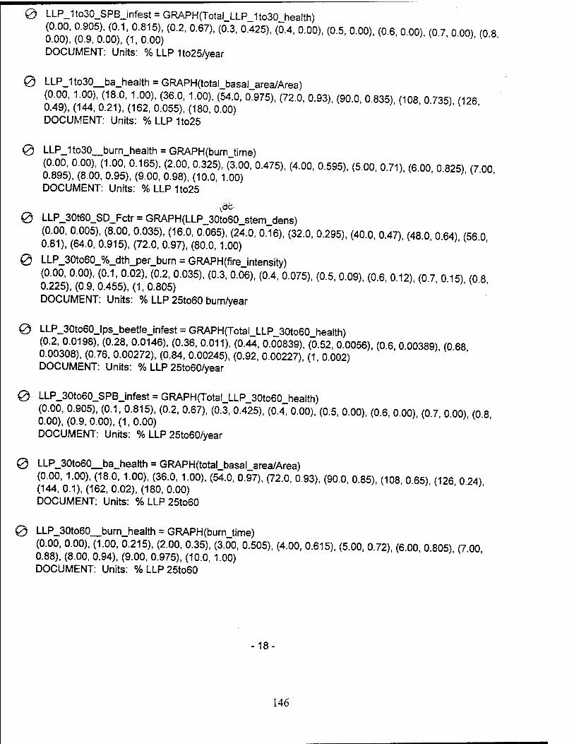
0 LLP_1to30_SPB_infest = GRAPH(Total_LLP_1to30_health)
£$: ÄS(0'2, °'67)'(0-3, °"425)' (°-4,^(0-5,0•00)•(0-6'000)'(07- °-oo)'(o-8' DOCUMENT: Units: % LLP 1to25/year
0 LLP_1to30_ba_health = GRAPH(total_basal_area/Area) (0.00, 1.00), (18.0, 1.00), (36.0, 1.00), (54.0, 0.975), (72.0, 0.93), (90.0, 0.835), (108 0 735) (126 0.49), (144, 0.21), (162, 0.055), (180, 0.00) ' ' '" U ' DOCUMENT: Units: % LLP 1to25
0 LLP_1to30_bum_health = GRAPH(burnJime) (0.00, 0.00), (1.00, 0.165), (2.00, 0.325), (3.00, 0.475), (4.00, 0.595), (5.00, 0.71), (6 00 0 825) (7 00 0.895), (8.00, 0.95), (9.00, 0.98), (10.0, 1.00) '' { ' DOCUMENT: Units: % LLP 1to25
■Kdc
0 LLP_30t60_SD_Fctr = GRAPH(LLP_30to60_stem_dens) (0.00, 0.005), (8.00, 0.035), (16.0, 0.065), (24.0, 0.16), (32.0, 0.295), (40.0, 0.47) (48 0 0 64) (56 0 0.81), (64.0, 0.915), (72.0, 0.97), (80.0, 1.00) ''" M '
0 LLP_30to60_%_dth_per_bum = GRAPH(fireJntensity) (0.00, 0.00), (0.1, 0.02), (0.2, 0.035), (0.3, 0.06), (0.4, 0.075), (0.5, 0.09), (0.6, 0 12) (0 7 0 15) (0 8 0.225), (0.9, 0.455), (1, 0.805) ' ' ' ;'{ ' DOCUMENT: Units: % LLP 25to60 burn/year
0 LLP_30to60_lps_beetle_infest = GRAPH(Total_LLP_30to60_health) (0.2, 0.0198), (0.28, 0.0146), (0.36, 0.011), (0.44, 0.00839), (0.52, 0.0056), (0.6 0 00389) (0 68 0.00308), (0.76, 0.00272), (0.84, 0.00245), (0.92, 0.00227), (1,0.002) ' DOCUMENT: Units: % LLP 25to60/year
0 LLP_30to60_SPB_infest = GRAPH(Total_LLP_30to60_health) (0.00, 0.905), (0.1, 0.815), (0.2, 0.67), (0.3, 0.425), (0.4, 0.00), (0.5, 0.00), (0.6, 0.00) (0 7 0 00) (0 8 0.00), (0.9, 0.00), (1, 0.00) h v ' DOCUMENT: Units: % LLP 25to60/year
0 LLP_30to60_ba_health = GRAPH(total_basal_area/Area) (0.00, 1.00), (18.0, 1.00), (36.0, 1.00), (54.0, 0.97), (72.0, 0.93), (90.0, 0.85), (108 0 65) (126 0 24) (144, 0.1), (162, 0.02), (180, 0.00) ' ' '' DOCUMENT: Units: %LLP25to60
0 LLP_30to60_burn_health = GRAPH(bumJime) (0.00, 0.00), (1.00, 0.215), (2.00, 0.35), (3.00, 0.505), (4.00, 0.615), (5.00, 0.72), (6.00 0 805) (7 00 0.88), (8.00, 0.94), (9.00, 0.975), (10.0, 1.00) ' DOCUMENT: Units: %LLP25to60
18
146
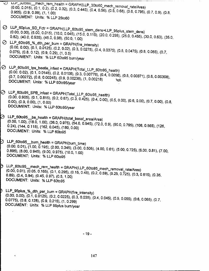
0.955), (0.9 0.99): a 1.00) ''<0'3' ^ (°A 0^ (0'5' °-68>> <P* ° W. (07, 0.9), (0.8, DOCUMENT: Units: %LLP25to60
0.82), (40.0, 0.935), (45.0 0.98)! (500 i 00) ''' °' °295)' (25'°' °'455»'<300' 063>. (35-0, 0 ^-6°t?95-%-dth-Per-''™ = GRAPH(fire intensity)
Ä ?ÄÄ(iaS| (°'3' ^ (°A ^ ^ °°^ «* -55), (0.7. DOCUMENT: Units: % LLP 60to95 burn/year
0 LLP_60to95_lps_beetle_infest = GRAPH(Total LLP 60to95 healtM
DOCUMENT: Units: % LLP 60to95/year ' ™
0 LLP_60to95_SPB_infest = GRAPH(Total_LLP_60to95 health)
£K ÄS,1;"^)(0-2' 067)-(0i' °-4"25)- ^°^ ^ *«*■ (0.6, 0.00), (0.7, 0.00), (0.8, DOCUMENT: Units: % LLP 60to95/year
3 LLnn?f-ba-health = GRAPH(total_basal area/Area)
ESS ÄÄ ÄÄ 0'm-(720'a9)'<900' °^ »«■ **«>. (1* DOCUMENT: Units: %LLP60to95
3 LLP_60to95_burn_health = GRAPH(burnJime)
ÄW«ÄawSo%"°*(400'a61)'<500' °^ (6-°°' ->■ ™ DOCUMENT: Units: %LLP60to95
DOCUMENT: Units: %LLP60to95
) LLP_95plus_%_dth_per_bum = GRAPH(fire_intensity)
ÄÄÄ ÄÄ0035'' «* «"* M «** «W 0.055). (0.7, DOCUMENT: Units: % LLP 95plus bum/year
19
147
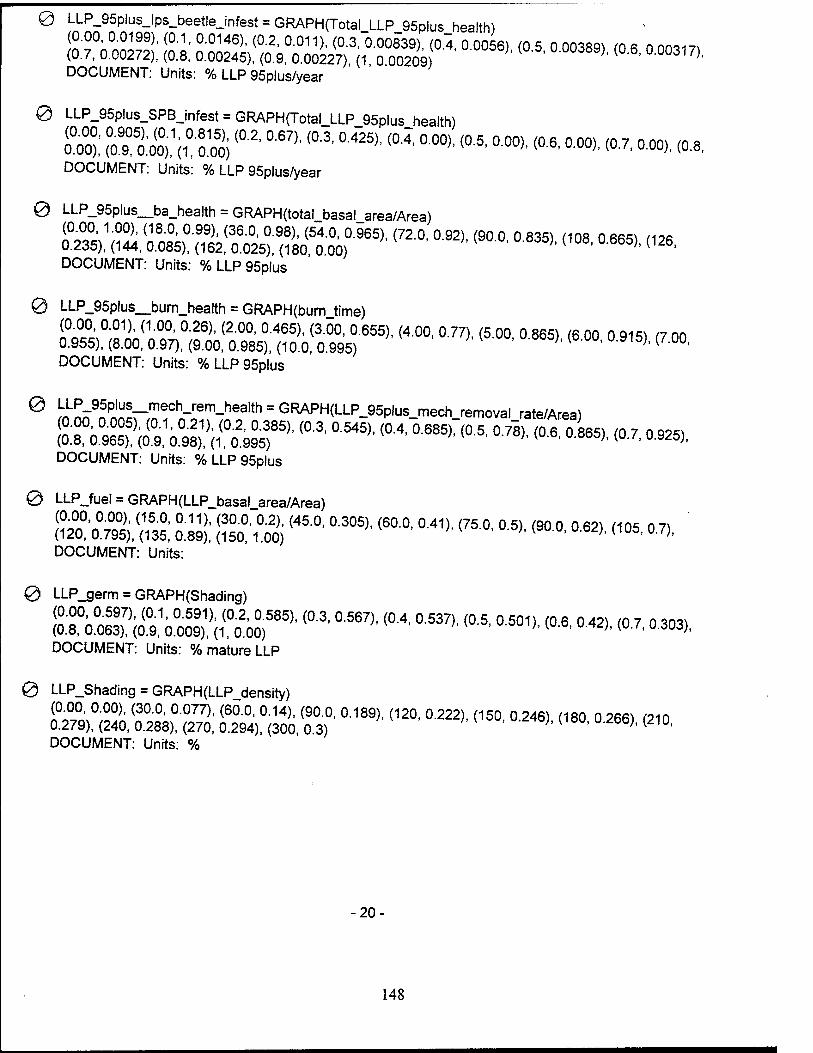
0 LLP_95plus_lps_beetle_infest = GRAPH(Total_LLP_95plus health)
SSÄ Ik »ÄÄA 00056)'(0-5' 000389>'«* °°M17>' DOCUMENT: Units: % LLP 95plus/year
0 LLP_95plus_SPB_infest = GRAPH(Total_LLP_95plus_health)
fm Z^OOU^ (0'2' °'67X (0"3' a4l5)'«* a0°>< <°-5' «■«»■ <0^ ^«». «"* 000). (C.8, DOCUMENT: Units: % LLP 95plus/year
0 LLP_95plus_ba_health = GRAPH(total_basal_area/Area)
^ÄÄTiTÄÄ^(720'a92)' (9° °' °-835»' ^ °^ «»■ DOCUMENT: Units: %LLP95pius
0 LLP_95p!us_burn_hea!th = GRAPH(burnJime)
sassÄ6551' (4o°' °m (5o°'om' (6o°' °'915)' (7°°' DOCUMENT: Units: % LLP 95p!us
0 J"nLnn9nnncwn!C«-rem-health = G^PH(Ll-P_95plus_mech_removal rate/Area)
^S&^^g»-(03'0545)-(0A 0685)-(0-5- **>■ ^ ° ^ *»- *■*>. DOCUMENT: Units: % LLP 95plus
0 LLP_fuei = GRAPH(LLP_basal_area/Area)
K2Ä £$ Ä (45'°' °'305)' <6°°' °'41'' <75'°' °-5>' (90'°' °'62>' <105' 07), DOCUMENT: Units:
0 LLP_germ = GRAPH(Shading)
!oTo0oe1)7\o(09:a0co9)1>ii(0o2oo,585)' (°'3' °^ ^ "^ ^ °m- (°'6' °'42)'(0'7°'303>' DOCUMENT: Units: % mature LLP
0 LLP_Shading = GRAPH(LLP_density)
MM EM (o a,0' °-m-(120' °-222)'<150'a246)'(180' °-266>' ™ DOCUMENT: Units: %
-20
148
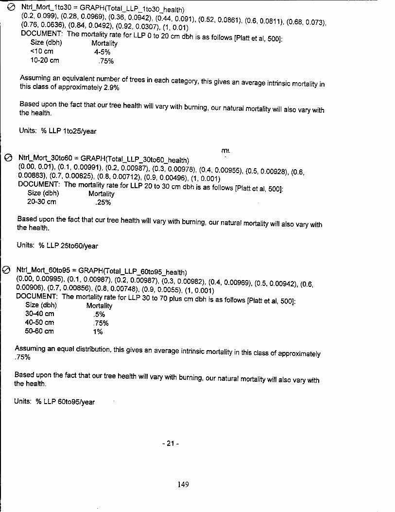
0 Ntrl_Mort_1to30 = GRAPH(Total_LLP_1to30_health) (0.2, 0.099), (0.28, 0.0969), (0.36, 0.0942), (0.44, 0.091), (0.52, 0 0861) (0 6 0 08111 (0 68 o n™ (0.76, 0.0636), (0.84, 0.0492), (0.92, 0.0307) (1 0 01) U ( ' °073)' D0?UM,w^: ThS m°?f'ity rate f°r LLP °t0 20 cm dbh is as foll°ws [Platt et al 500]- Size (dbh) Mortality J-
<10cm 4-5% 10-20 cm .75%
SSi^:% °f ^ " ^ Categ0ry'thiS *- 3n ««■• "*-c mortaHty in
fhe'heaX"** ** ** ™*"* ^ ™" ^ ^ bUminQ' °Ur natUral morta^ wi" also varV «*h
Units: % LLP 1to25/year
(TIL
0 Ntrl_Mort_30to60 = GRAPH(Total_LLP_30to60_health) (0.00, 0.01), (0.1, 0.00991), (0.2, 0.00987), (0.3, 0.00978), (0.4, 0.00955) (0 5 0 00928) (Q 6 0.00883), (0.7, 0.00825), (0.8, 0.00712), (0.9, 0.00496), (1, 0.001) ''(
DOCUMENT: The mortality rate for LLP 20 to 30 cm dbh is as follows [Platt et al 500V Size (dbh) Mortality 20-30 cm .25%
theShealtPh0n ** ** ** ^ ^ ^'^ Wi" ^ W*h bUming' °Ur natural mort*lit* wi" also varV with
Units: % LLP 25to60/year
0 Ntrl_Mort_60to95 = GRAPH(Total_LLP_60to95_health) (O00, 0.00995), (0.1, 0.00987), (0.2, 0.00987), (0.3, 0.00982), (0.4, 0.00969) (0 5 0 00942) (0 6 0.00906), (0.7, 0.00856), (0.8, 0.00748), (0.9, 0.0055), (1, 0.001) }'( ' DOCUMENT: The mortality rate for LLP 30 to 70 plus cm dbh is as follows [Platt et al 500V
Size (dbh) Mortality ' J' 30-40 cm .5% 40-50 cm .75% 50-60 cm 1%
Assuming an equal distribution, this gives an average intrinsic mortality in this class of approximately
^health0" ** ** ** ^ *** ^^ *"' ^ ^ bUmin9, °Ur natural mortal^ wi" also varV with
Units: % LLP 60to95/year
21 -
149
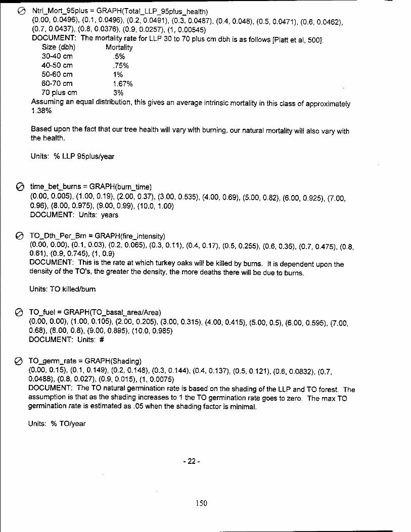
0 Ntrl_Mort_95plus = GRAPH(Total_LLP_95plus_health) (0.00, 0.0496), (0.1, 0.0496), (0.2, 0.0491), (0.3, 0.0487), (0.4, 0.048), (0.5, 0.0471), (0.6, 0 0462) (0.7, 0.0437), (0.8, 0.0376), (0.9, 0.0257), (1, 0.00545) DOCUMENT: The mortality rate for LLP 30 to 70 plus cm dbh is as follows [Platt et al, 500]:
Size (dbh) Mortality 30-40 cm .5% 40-50 cm .75% 50-60 cm 1% 60-70 cm 1.67% 70 plus cm 3%
Assuming an equal distribution, this gives an average intrinsic mortality in this class of approximately 1.38%
Based upon the fact that our tree health will vary with burning, our natural mortality will also vary with the health.
Units: % LLP 95plus/year
0 time_bet_burns = GRAPH(bum_time) (0.00, 0.005), (1.00, 0.19), (2.00, 0.37), (3.00, 0.535), (4.00, 0.69), (5.00, 0.82), (6.00, 0.925), (7.00 0.96), (8.00, 0.975), (9.00, 0.99), (10.0, 1.00) DOCUMENT: Units: years
0 TO_Dth_Per_Brn = GRAPH(fire_intensity) (0.00, 0.00), (0.1, 0.03), (0.2, 0.065), (0.3, 0.11), (0.4, 0.17), (0.5, 0.255), (0.6, 0.35), (0.7, 0.475), (0.8 0.61), (0.9,0.745), (1,0.9) DOCUMENT: This is the rate at which turkey oaks will be killed by burns. It is dependent upon the density of the TO's, the greater the density, the more deaths there will be due to burns.
Units: TO killed/burn
0 TOJuel = GRAPH(TO_basal_area/Area) (0.00, 0.00), (1.00, 0.105), (2.00, 0.205), (3.00, 0.315), (4.00, 0.415), (5.00, 0.5), (6.00, 0.595), (7.00, 0.68), (8.00, 0.8), (9.00, 0.895), (10.0, 0.985) DOCUMENT: Units: #
0 TO_germ_rate = GRAPH(Shading) (0.00, 0.15), (0.1, 0.149), (0.2, 0.148), (0.3, 0.144), (0.4, 0.137), (0.5, 0.121), (0.6, 0.0832), (0.7, 0.0488), (0.8, 0.027), (0.9, 0.015), (1, 0.0075) DOCUMENT: The TO natural germination rate is based on the shading of the LLP and TO forest. The assumption is that as the shading increases to 1 the TO germination rate goes to zero. The max TO germination rate is estimated as .05 when the shading factor is minimal.
Units: % TO/year
-22-
150
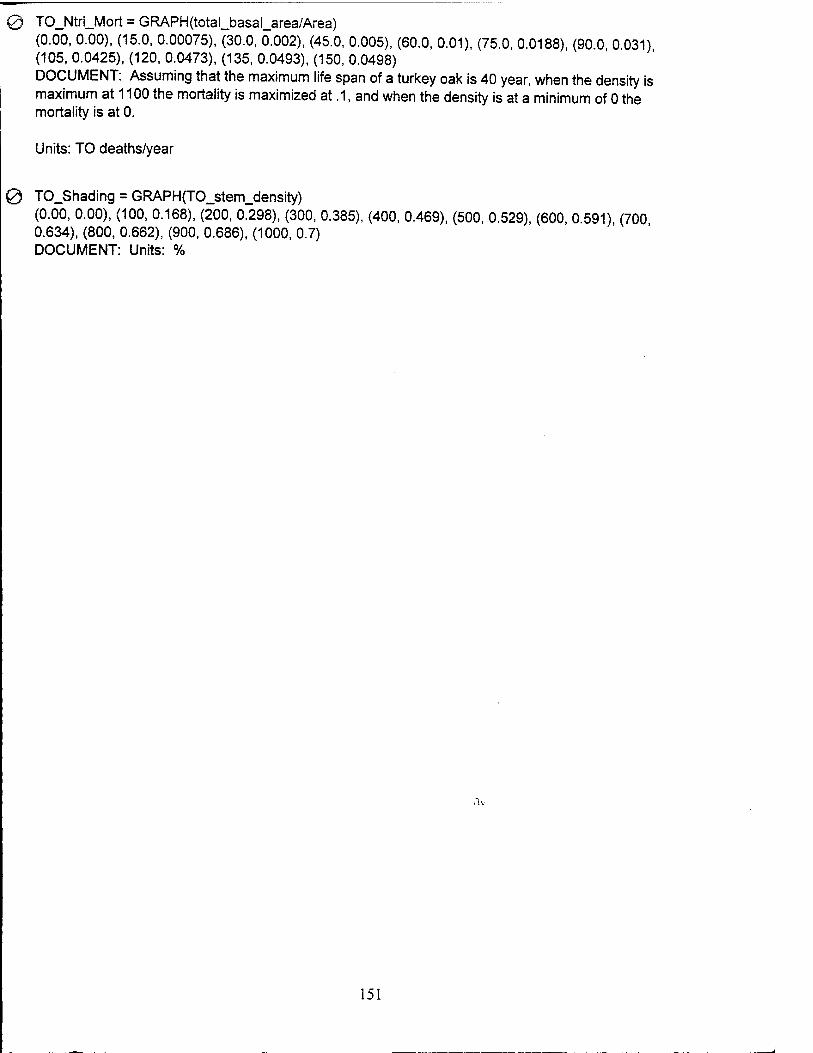
0 TO_Ntrl_Mort = GRAPH(total_basal_area/Area) (0.00, 0.00), (15.0, 0.00075), (30.0, 0.002), (45.0, 0.005), (60.0, 0.01), (75.0, 0.0188), (90 0 0 031) (105, 0.0425), (120, 0.0473), (135, 0.0493), (150, 0.0498) DOCUMENT: Assuming that the maximum life span of a turkey oak is 40 year, when the density is maximum at 1100 the mortality is maximized at .1, and when the density is at a minimum of 0 the mortality is at 0.
Units: TO deaths/year
0 TO_Shading = GRAPH(TO_stem_density) (0.00, 0.00), (100, 0.168), (200, 0^298), (300, 0.385), (400, 0.469), (500, 0.529), (600, 0.591) (700 0.634), (800, 0.662), (900, 0.686), (1000, 0.7) DOCUMENT: Units: %
151