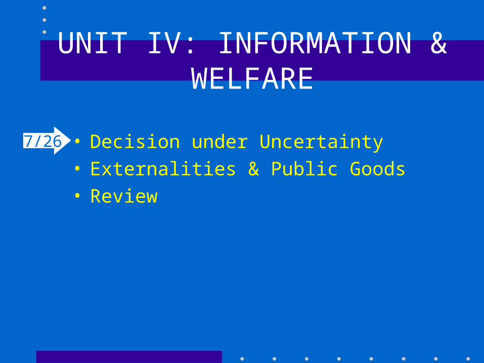
UNIT IV: INFORMATION & WELFARE

• Decision under Uncertainty• Externalities & Public Goods • Review

7/26

Cartel Enforcement

Consider a market in which two identical firms can produce a good with a marginal cost of $1 per unit. The market demand function is given by:

P = 7 – Q

Assume that the firms choose prices. If the two firms choose different prices, the one with the lower price gets all the customers; if they choose the same price, they split the market demand.

What is the Nash Equilibrium of this game?

Cartel Enforcement

Consider a market in which two identical firms can produce a good with a marginal cost of $1 per unit. The market demand function is given by:

P = 7 – Q

Now suppose that the firms compete repeatedly, and each firm attempts to maximize the discounted value of its profits ( < 1).

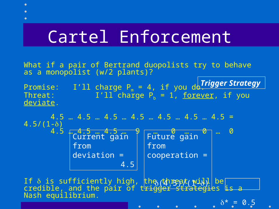
What if this pair of Bertrand duopolists try to behave as a monopolist (w/2 plants)?

Cartel Enforcement

What if a pair of Bertrand duopolists try to behave as a monopolist (w/2 plants)?

P = 7 – Q; TCi = qi

Monopoly Bertrand Duopoly

= TR – TC Q = q1 + q2 = PQ – Q Pb = MC = 1; Qb = 6= (7-Q)Q - Q = 7Q - Q2 - Q

FOC: 7-2Q-1 = 0 => Qm = 3; Pm = 4

w/2 plants: q1 = q2 = 1.5 q1 = q2 = 31= 2 = 4.5 = 2 = 0

Cartel Enforcement

What if a pair of Bertrand duopolists try to behave as a monopolist (w/2 plants)?

Promise: I’ll charge Pm = 4, if you do.Threat: I’ll charge Pb = 1, forever, if you deviate.

4.5 … 4.5 … 4.5 … 4.5 … 4.5 … 4.5 … 4.5 = 4.5/(1-)4.5 … 4.5 … 4.5 … 9 … 0 … 0 … 0

If is sufficiently high, the threat will be credible, and the pair of trigger strategies is a Nash equilibrium.

* = 0.5

Trigger Strategy

Current gain from deviation =

4.5

Future gain from cooperation =

(4.5)/(1-)

Decision under Uncertainty

In UNIT I we assumed that consumers have perfect information about the possible options they face (their income and prices); and about the utility consequences of their choices (their preferences).

Now, we will ask whether our model can be extended to deal with more realistic cases in which decisions are made without perfect information.

We will also ask how imperfect (asymmetric) information affects market outcomes and their welfare consequences.

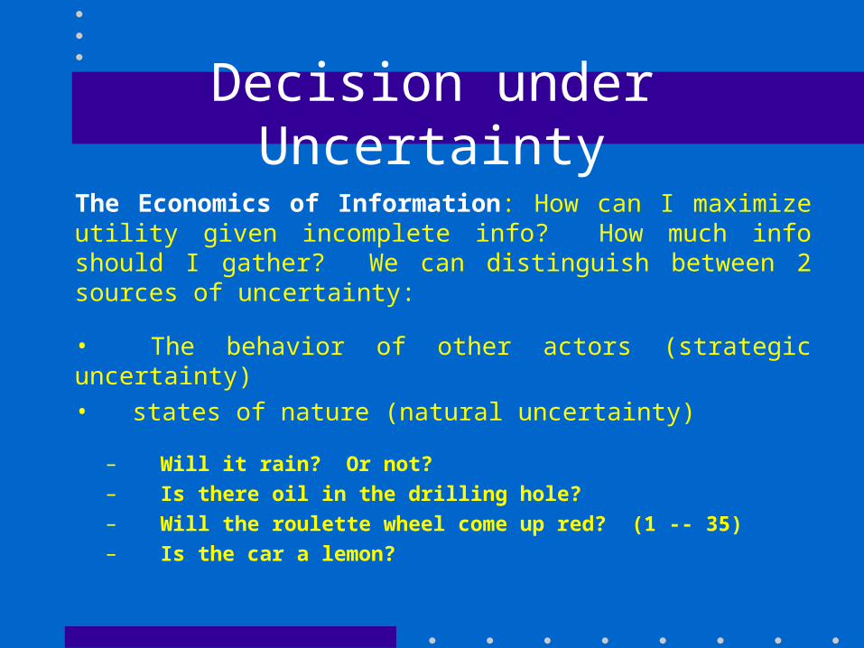
Decision under Uncertainty

The Economics of Information: How can I maximize utility given incomplete info? How much info should I gather? We can distinguish between 2 sources of uncertainty:

• The behavior of other actors (strategic uncertainty)

• states of nature (natural uncertainty)

– Will it rain? Or not?

– Is there oil in the drilling hole?

– Will the roulette wheel come up red? (1 -- 35)

– Is the car a lemon?

Decision under Uncertainty

• Expected Value v. Expected Utility• Risk Preferences• Reducing Risk: Insurance• Contingent Consumption• Adverse Selection (and Moral Hazard)

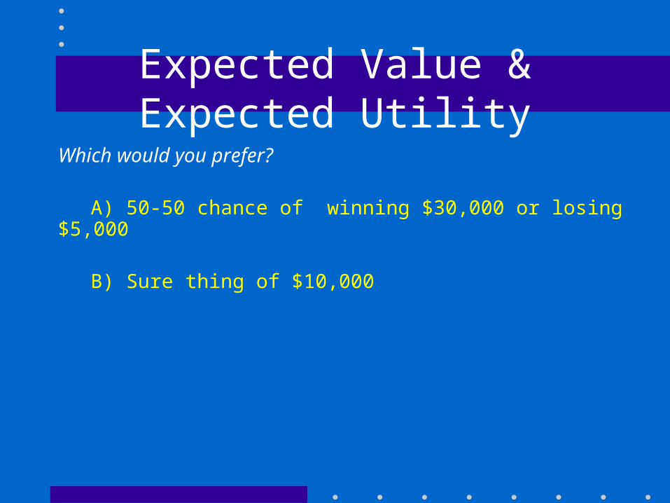
Expected Value & Expected UtilityWhich would you prefer?

A) 50-50 chance of winning $30,000 or losing $5,000

B) Sure thing of $10,000

How much would you be willing to pay for the chance to win $2n if the head comes up on nth flip?

2(1/2) + 4(1/4) + … = 1 + 1 + … =

Expected Value & Expected Utility

How much would you be willing to pay for the chance to win $2n if a heads comes up on nth flip?

Expected Value (EV): the sum of the value (V) of each possible state, weighted by the probability () of that state occurring.

On 1 flip:

(H) = ½ (2) + 4(1/4) + … = 1 + 1 + … =

Expected Value & Expected Utility

How much would you be willing to pay for the chance to win $2n if a heads comes up on nth flip?

Expected Value (EV): the sum of the value (V) of each possible state, weighted by the probability () of that state occurring.

On 1 flip:

EV = (V)H = (½)2 + 4(1/4) + … = 1 + 1 + … =

Expected Value & Expected Utility

How much would you be willing to pay for the chance to win $2n if a heads comes up on nth flip?

Expected Value (EV): the sum of the value (V) of each possible state, weighted by the probability () of that state occurring.

On nth flip:

EV(Hn) = ½n(2n) + 4(1/4) + … = 1 + 1 + … =

Expected Value & Expected UtilityHow much would you be willing to pay for the chance to win $2n if a heads comes up on nth flip?

Expected Value (EV): the sum of the value (V) of each possible state, weighted by the probability () of that state occurring.

On nth flip:

EV(Hn) = ½n(2n) + 4(1/4) + … = 1 + 1 + … =

½ ½

¼ ¼

88

EV(H)=½(2)+(1/4)4+(1/8)8Flip 1: Win $2

Flip 2: Win $4

Flip 3: Win $8

H T

H T

H T

11

Expected Value & Expected Utility

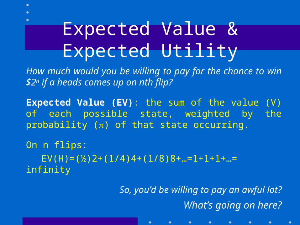
How much would you be willing to pay for the chance to win $2n if a heads comes up on nth flip?

Expected Value (EV): the sum of the value (V) of each possible state, weighted by the probability () of that state occurring.

On n flips:

EV(H)=(½)2+(1/4)4+(1/8)8+…=1+1+1+…= infinity

So, you’d be willing to pay an awful lot?

What’s going on here?

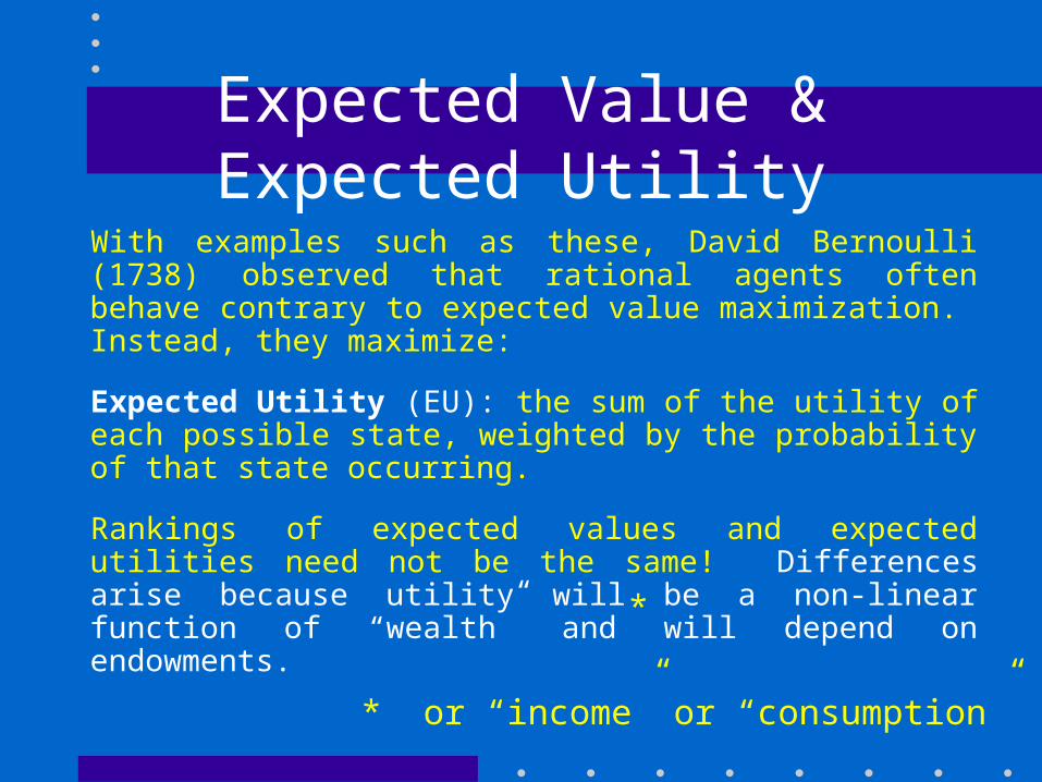
Expected Value & Expected UtilityWith examples such as these, David Bernoulli (1738) observed that rational agents often behave contrary to expected value maximization. Instead, they maximize:

Expected Utility (EU): the sum of the utility of each possible state, weighted by the probability of that state occurring.

EU = 1(U(s1)) + 2(U(s2)) + … n(U(sn))

Where is the probability of that state occurring. arise because utility will be a non-linear function of “wealth”.

Expected Value & Expected UtilityWith examples such as these, David Bernoulli (1738) observed that rational agents often behave contrary to expected value maximization. Instead, they maximize:

Expected Utility (EU): the sum of the utility of each possible state, weighted by the probability of that state occurring.

Rankings of expected values and expected utilities need not be the same! Differences arise because utility will be a non-linear function of “wealth” and will depend on endowments.

* or “income” or “consumption”

*

Expected Value & Expected Utility

Diminishing Marginal Utility: The intrinsic worth of wealth increases with wealth, but at a diminishing rate.

5 10 15 W

UU(15)

U(10)

U(5)

von Neumann-Morgenstern Utility Indexes

MU = ½W-½ U = W½

MU = 1/W U = lnW

For 2 states:

EU = (U(Wi)) + (1-)(U(Wj))

MRS = (/(1-))MUi/MUj

Risk Preferences

A risk averse consumer will prefer a certain income to a risky income with the same expected value.

5 CE 10 15 W

UU(15)

U(10)

U(5)

.5U(5) +.5U(15)

The chord represents the chance to

win $5 or $15.

Risk Preferences

A risk averse consumer will prefer a certain income to a risky income with the same expected value.

5 CE 10 15 W

UU(15)

U(10)

U(5)

.5U(5) +.5U(15) Certainty Equivalent (CE) of an equal chance of

winning $5 and $15

Risk Premium = 10 – CE

Risk Preferences

A risk loving consumer will prefer a risky income to a certain income with the same expected value.

5 CE 10 15 W

U

U(15)

.5U(5) +.5U(15)

U(5) U(10)

Risk Preferences

A risk neutral consumer is indifferent between a risky income and a certain income with the same expected value.

5 CE 10 15 W

U

U(15)

U(10)

U(5)

Risk Preferences

A risk neutral consumer is indifferent between a risky income and a certain income with the same expected value.

5 CE 10 15 W

U

U(15)

U(10)

U(5)

Do any of these cases violate any of our assumptions about well-behaved preferences?

Draw a set of indifference curves for each case.

Risk and Insurance

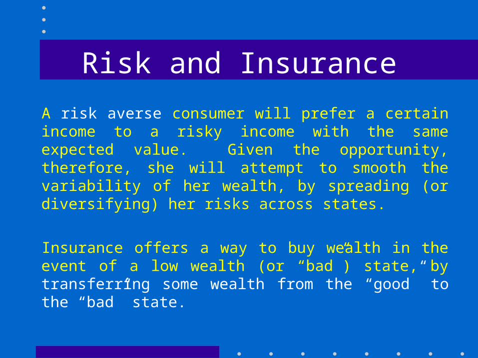
A risk averse consumer will prefer a certain income to a risky income with the same expected value. Given the opportunity, therefore, she will attempt to smooth the variability of her wealth, by spreading (or diversifying) her risks across states.

Insurance offers a way to buy wealth in the event of a low wealth (or “bad”) state, by transferring some wealth from the “good” to the “bad” state.

Risk and Insurance

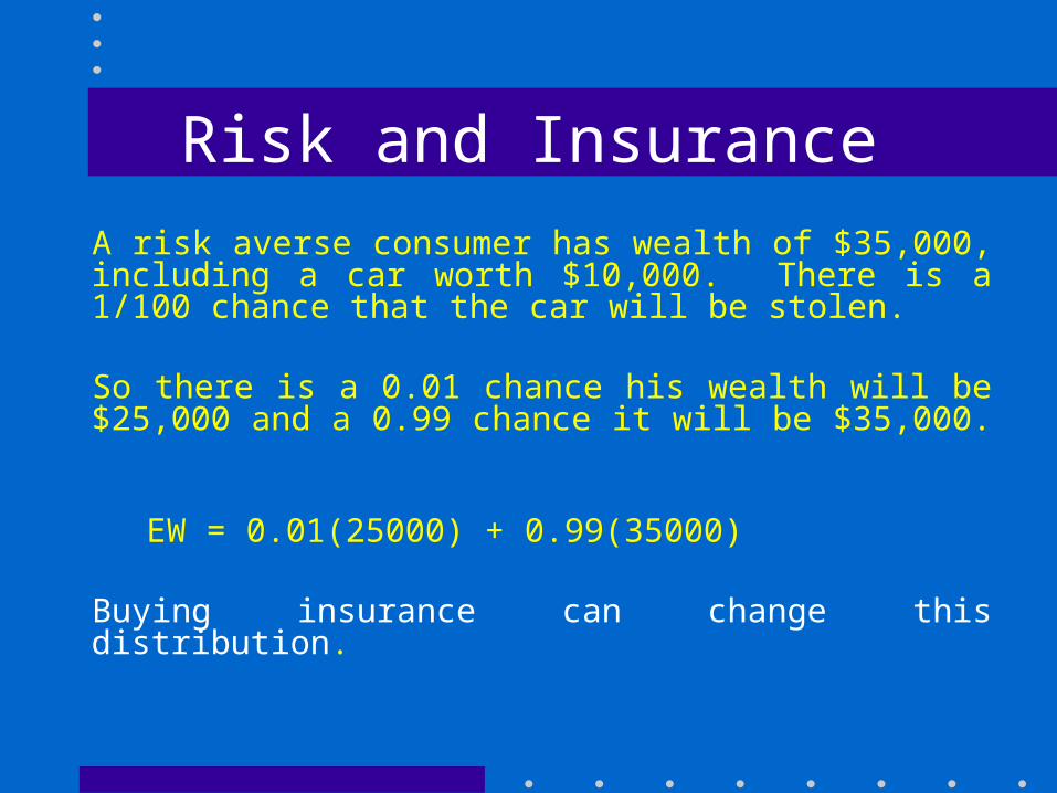
A risk averse consumer has wealth of $35,000, including a car worth $10,000. There is a 1/100 chance that the car will be stolen.

So there is a 0.01 chance his wealth will be $25,000 and a 0.99 chance it will be $35,000.

EW = 0.01(25000) + 0.99(35000)

Buying insurance can change this distribution.

Risk and Insurance

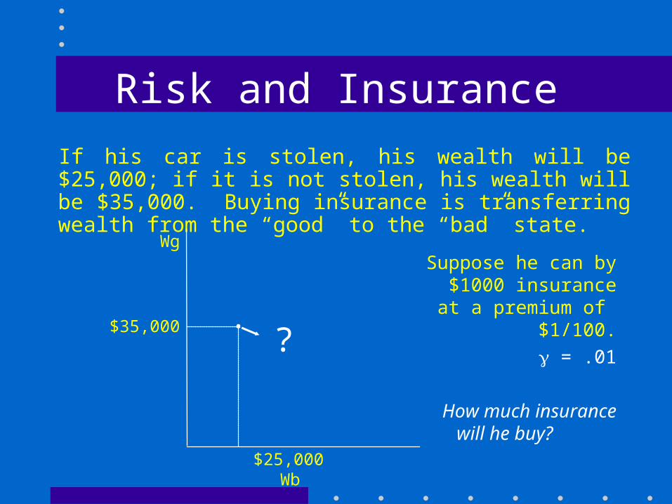
If his car is stolen, his wealth will be $25,000; if it is not stolen, his wealth will be $35,000. Buying insurance is transferring wealth from the “good” to the “bad” state.

$25,000 Wb

Wg

$35,000(35,000 – 10)

(25,000 + 1000 -10)

Suppose he can by $1000 insurance at a premium of $1/100.

= .01

How much insurance will he buy?he buy?

Not to scale

Risk and Insurance

If his car is stolen, his wealth will be $25,000; if it is not stolen, his wealth will be $35,000. Buying insurance is transferring wealth from the “good” to the “bad” state.

$25,000 Wb

Wg

$35,000

Suppose he can by $1000 insurance at a premium of $1/100.

= .01

How much insurance will he buy?he buy?

?

Risk and Insurance

If his car is stolen, his wealth will be $25,000; if it is not stolen, his wealth will be $35,000. Buying insurance is transferring wealth from the “good” to the “bad” state.

$25,000 Wb

Wg

$35,000

Given the chance to buy insurance at an “actuarily fair” price

(i.e., = ), a risk averse consumer will

fully insure.

Equalizing wealth across states.

he buy?

34,900

34,900

Certainty Line

Risk and Insurance

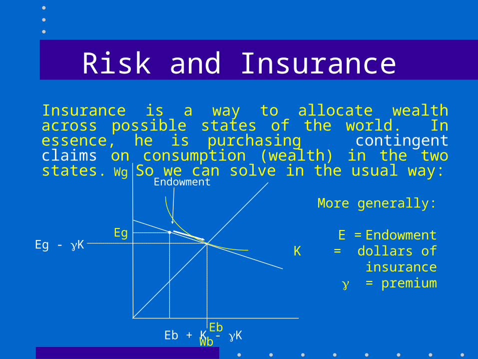
Insurance is a way to allocate wealth across possible states of the world. In essence, he is purchasing contingent claims on consumption (wealth) in the two states. So we can solve in the usual way:

Eb Wb

Wg

Eg

More generally:

E = EndowmentK = dollars of insurance

= premium

?

Eg - K

Eb + K - K

Endowment

Contingent Consumption

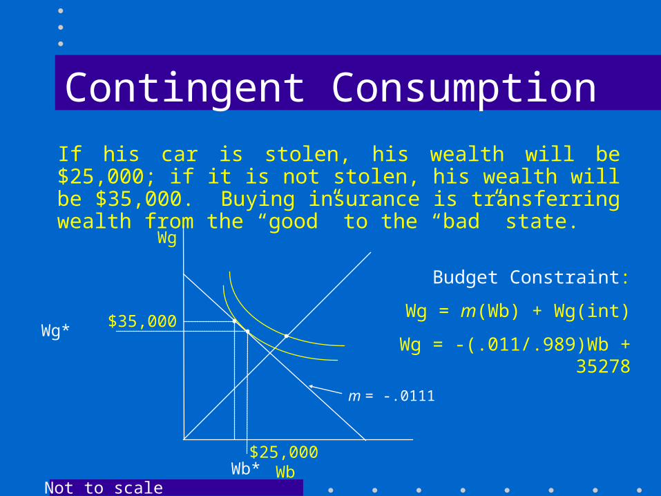
If his car is stolen, his wealth will be $25,000; if it is not stolen, his wealth will be $35,000. Buying insurance is transferring wealth from the “good” to the “bad” state.

$25,000 Wb

Wg

$35,00035000 - k

25,000 + K - K

Now suppose the premium rises to $1.10/100 ( = .011).

His vN-M Index: U = lnW

How much insurance will he buy?

Endowment

Contingent Consumption

If his car is stolen, his wealth will be $25,000; if it is not stolen, his wealth will be $35,000. Buying insurance is transferring wealth from the “good” to the “bad” state.

$25,000 Wb

Wg

$35,000

Slope(m) = Wg/Wb

= -K/(K-K)

= -/(1-)

= Pb

1- = Pg

Not to scale

m = -Pb/Pg

Contingent Consumption

If his car is stolen, his wealth will be $25,000; if it is not stolen, his wealth will be $35,000. Buying insurance is transferring wealth from the “good” to the “bad” state.

$25,000 Wb

Wg

$35,000Wg*

Wb*

What is his budget constraint?

Not to scale

m = -.0111

Contingent Consumption

If his car is stolen, his wealth will be $25,000; if it is not stolen, his wealth will be $35,000. Buying insurance is transferring wealth from the “good” to the “bad” state.

$25,000 Wb

Wg

$35,000Wg*

Wb*

Budget Constraint:

Wg = m(Wb) + Wg(int)

Wg = -(.011/.989)Wb + 35278

Not to scale

m = -.0111

Contingent Consumption

If his car is stolen, his wealth will be $25,000; if it is not stolen, his wealth will be $35,000. Buying insurance is transferring wealth from the “good” to the “bad” state.

$25,000 Wb

Wg

$35,000Wg*

Wb*

U = lnW

EU = (U(Wb)) + (1-)(U(Wg))

MRS = (/(1-))MUb/MUg = (.01/.99)(Wg/Wb)

= P(Wb)/P(Wg)= /(1-)

Not to scale

Contingent Consumption

If his can is stolen, his wealth will be $25,000; if it is not stolen, his wealth will be $35,000. Buying insurance is transferring wealth from the “good” to the “bad” state.

$25,000 Wb

Wg

$35,000Wg*

Wb*

MRS = (.01/.99)(Wg/Wb)

Pb/Pg = /(1-)

MRS = Pb/Pg => Wb = .909Wg

Wg = -(.011/.989)Wb + 35278

Wg = $ 34925

Not to scale

Contingent Consumption

If his can is stolen, his wealth will be $25,000; if it is not stolen, his wealth will be $35,000. Buying insurance is transferring wealth from the “good” to the “bad” state.

$25,000 Wb

Wg

$35,000Wg*=34925

Wb*=31743

Wg = $ 34925

So he pays $75 for $6818 of ins

Not to scale

Contingent Consumption

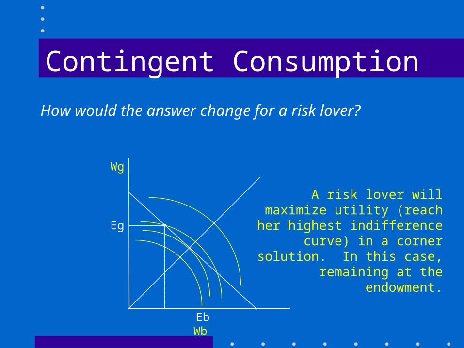
How would the answer change for a risk lover?

Eb Wb

Wg

Eg

A risk lover will maximize utility (reach her highest indifference curve) in a corner solution. In

this case, remaining at the endowment.

Adverse Selection

Consider the market for drivers insurance:

“Good” drivers have accidents with prob = 0.2“Bad” = 0.8

Good and bad drivers are equally distributed in population.

At the actuarially fair price of $0.50/$1 coverage:– for good drivers price is too high -> don’t insure– for bad too low -> insure

Bad drivers are “selected in”; good are “selected out”

What price would an actuarially fair insurance company charge?

Adverse Selection

Consider the market for drivers insurance:

“Good” drivers have accidents with prob = 0.2“Bad” = 0.8

Good and bad drivers are equally distributed in population.

At the actuarially fair price of $0.50/$1 coverage:– for good drivers price is too high -> don’t insure– for bad too low -> insure

Bad drivers are “selected in”; good are “selected out”

Driver quality is a hidden characteristic

Asymmetric Information

Acquiring a Company

BUYER represents Company A (the Acquirer), which is currently considering make a tender offer to acquire Company T (the Target) from SELLER. BUYER and SELLER are going to be meeting to negotiate a price.

Company T is privately held, so its true value is known only to SELLER. Whatever the value, Company T is worth 50% more in the hands of the acquiring company, due to improved management and corporate synergies. BUYER only knows that its value is somewhere between 0 and 100 ($/share), with all values equally likely.

Source: M. Bazerman

Acquiring a Company

What offer should Buyer make?

Acquiring a Company

$0 10-15 20-25 30-35 40-45 50-55 60-65 70-75 80-85 90-95

5

Source: Bazerman, 1992

9

1 0

4 4 7

27

18

45

123 BU MBA Students

Similar results from

MIT Master’s Candidates

CPA; CEOs.

Offers

Acquiring a Company OFFER VALUE ACCEPT OR VALUE GAIN OR

TO SELLER REJECT TO BUYER LOSS (O) (s) (3/2 s = b) (b - O) $60 $0 A $0 $-60

10 A 15 -45 20 A 30 -30 30 A 45 -15 40 A 60 0 50 A 75 15 60 R - - 70 R - -

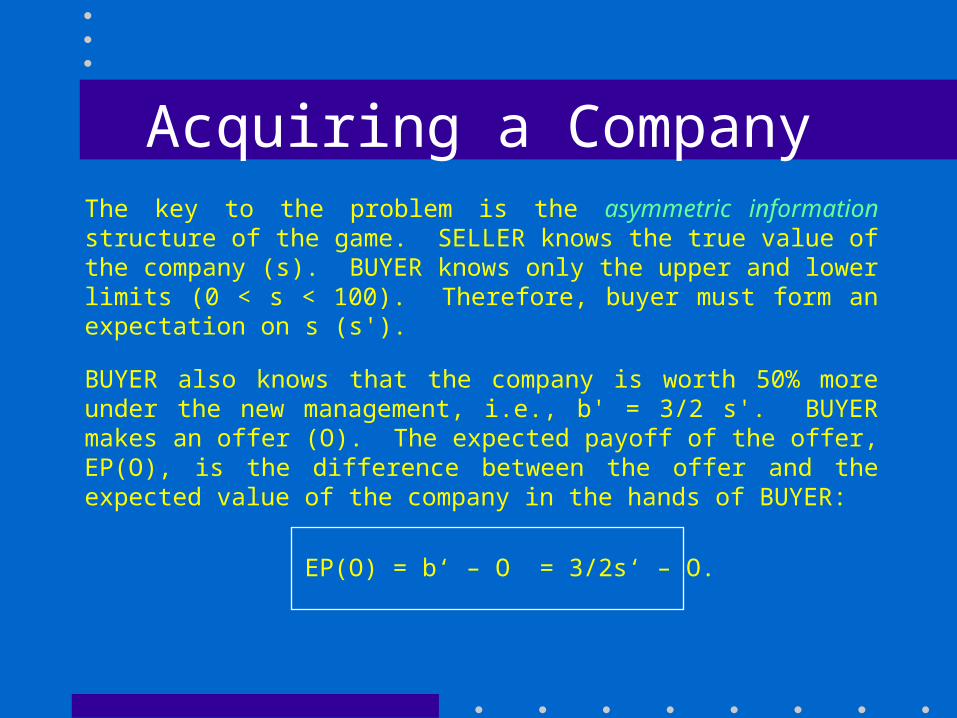
Acquiring a CompanyThe key to the problem is the asymmetric information structure of the game. SELLER knows the true value of the company (s). BUYER knows only the upper and lower limits (0 < s < 100). Therefore, buyer must form an expectation on s (s').

BUYER also knows that the company is worth 50% more under the new management, i.e., b' = 3/2 s'. BUYER makes an offer (O). The expected payoff of the offer, EP(O), is the difference between the offer and the expected value of the company in the hands of BUYER:

EP(O) = b‘ – O = 3/2s‘ – O.

Acquiring a CompanyBUYER wants to maximize her payoff by offering the smallest amount (O) she expects will be accepted:

EP(O) = b‘ – O = 3/2s‘ – O.

O = s' + . Seller accepts if O > s.

Now consider this: Buyer has formed her expectation based on very little information. If Buyer offers O and Seller accepts, this considerably increases Buyer’s information, so she can now update her expectation on s.

How should Buyer update her expectation, conditioned on the new information that s < O?  

Acquiring a CompanyBUYER wants to maximize her payoff by offering the smallest amount (O) she expects will be accepted:

EP(O) = b‘ – O = 3/2s‘ – O.

O = s' + . Seller accepts if O > s.

Let’s say BUYER offers $50. If SELLER accepts, BUYER knows that s cannot be greater than (or equal to) 50, that is: 0 < s < 50. Since all values are equally likely, s''/(s < O) = 25. The expected value of the company to BUYER (b'' = 3/2s'' = 37.50), which is less than the 50 she just offered to pay. (EP(O) = - 12.5.) When SELLER accepts, BUYER gets a sinking feeling in the pit of her stomach.

THE WINNER’S CURSE!

Acquiring a CompanyBUYER wants to maximize her payoff by offering the smallest amount (O) she expects will be accepted:

EP(O) = b‘ – O = 3/2s‘ – O.

O = s' + . Seller accepts if O > s.

Generally: EP(O) = O - ¼s' (-). EP is negative for all values of O.

THE WINNER’S CURSE!

Acquiring a Company

• The high level of uncertainty swamps the potential gains available, such that value is often left on the table, i.e., on average the outcome is inefficient.

• Under these particular conditions, BUYER should not make an offer.

• SELLER has an incentive to reveal some information to BUYER, because if BUYER can reduce the uncertainty, she may make an offer that leaves both players better off.

Adverse Selection

• Lemons (Akerlof 1970): Buyers of used cars can’t distinguish between high and low quality cars (lemons); the price of used cars reflects this uncertainty; and the price is lower than high quality cars are worth. Thus owners of high quality cars won’t choose to sell their cars at the market price; eventually, only (mostly) lemons will be sold on the used car market.  

• Sellers of high-quality products can use means to certify their value: Appraisals; audits; “reputable” agents; brand names.

 

Moral Hazard

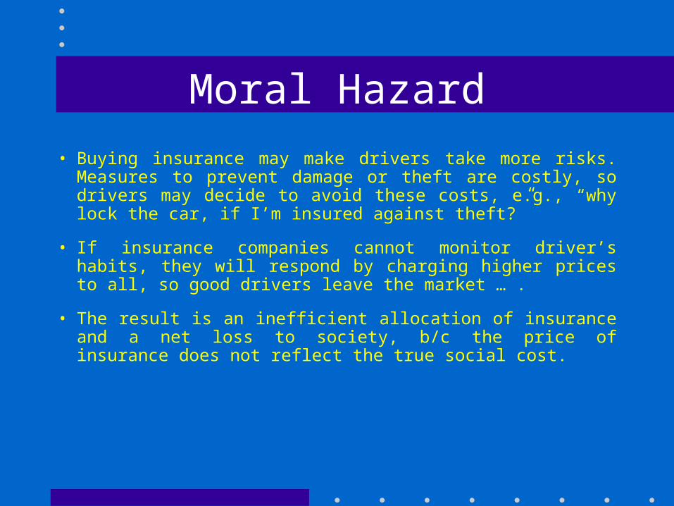
• Buying insurance may make drivers take more risks. Measures to prevent damage or theft are costly, so drivers may decide to avoid these costs, e.g., “why lock the car, if I’m insured against theft?”

• If insurance companies cannot monitor driver’s habits, they will respond by charging higher prices to all, so good drivers leave the market … .

• The result is an inefficient allocation of insurance and a net loss to society, b/c the price of insurance does not reflect the true social cost.

Next Time

7/28 Externalities and Public Goods

Pindyck and Rubenfeld, Ch 18.

Besanko, Ch. 17.