unit ii analysis of continuous time...
TRANSCRIPT
Page 1 of 31
NH-67, TRICHY MAIN ROAD, PULIYUR, C.F. – 639 114, KARUR DT.
DEPARTMENT OF ELECTRONICS AND COMMUNICATION ENGINEERING
COURSE MATERIAL
Subject Name : Signals and Systems Class/Sem : BE(ECE) / III
Subject Code : EC 2204 Staff name : G.Vijayakumari
Unit II ANALYSIS OF CONTINUOUS TIME SIGNALS
Fourier series analysis - Spectrum of C.T. signals - Fourier Transform
and Laplace Transform in Signal Analysis.
Objective:
The main objective of this unit is that students will be able to
understand, the definition of Fourier series, different ways of Fourier series
representation, calculation of power using parsevals theorem, properties of
Fourier series, the definition of Fourier Transform, the properties of Fourier
Transform The definition of Laplace Transforms, properties of Laplace
transforms, examples of Laplace Transforms, example for deriving Laplace
Transform from waveforms.
Keywords: Continuous Time Signals, Fourier series analysis, Fourier
Transform, parsevals Theorem, Laplace Transform.

Page 2 of 31
Contents:
2.1 Fourier Series representation of Periodic Signals
2.2 Dirichlet Conditions for convergence of Fourier series.
2.3 Properties of Fourier series
2.4 Fourier Transform
2.5 Dirichlet Conditions for convergence of Fourier Transform.
2.6 Properties of Fourier Transform
2.7 Laplace Transform
2.8 Properties of Laplace Transform
2.9 Sampling
2.1 Fourier Series representation of Periodic Signals
Consider a periodic signal x(t) with fundamental period T, i.e.
Then the fundamental frequency of this signal is defined as the reciprocal of
the fundamental period, so that
Under certain conditions, a periodic signal x(t) with period T can be
expressed as a linear combination of sinusoidal signals of discrete
frequencies, which are multiples of the fundamental frequency of x(t).
Page 3 of 31
Further, sinusoidal signals are conveniently represented in terms of complex
exponential signals. Hence, we can express the periodic signal in terms of
complex exponentials, i.e.
Such a representation of a periodic signal as a combination of complex
exponentials of discrete frequencies, which are multiples of the fundamental
frequency of the signal, is known as the Fourier Series Representation of the
signal.
Frequency Domain Representation
From the above discussion, we can say that a periodic signal whose
Fourier Series Expansion exists, can be represented uniquely in terms of it's
Fourier co-efficients. These co-efficients correspond to particular multiples
of the fundamental frequency of the signal. Thus, the signal may be
equivalently represented as a discrete signal on the frequency axis.
This is called the Frequency domain representation of the signal.
We next discuss the conditions under which the Fourier Expansion is valid.
2.2 Convergence of Fourier series (Dirichlet’s conditions):
1) x(t) should be absolutely integrable over a period.
2) x(t) should have only a finite number of discontinuities over one
period. Furthermore, each of these discontinuities must be finite.
Page 4 of 31
3) The signal x(t) should have only a finite number of maxima and
minima in one period.
If the signal satisfies the above conditions, then at all points where the
signal is continuous, the Fourier Series converges to the signal.
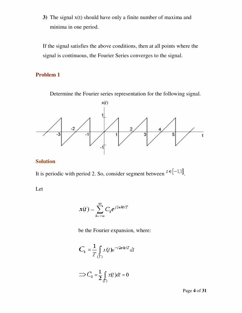
Problem 1
Determine the Fourier series representation for the following signal.
Solution
It is periodic with period 2. So, consider segment between .
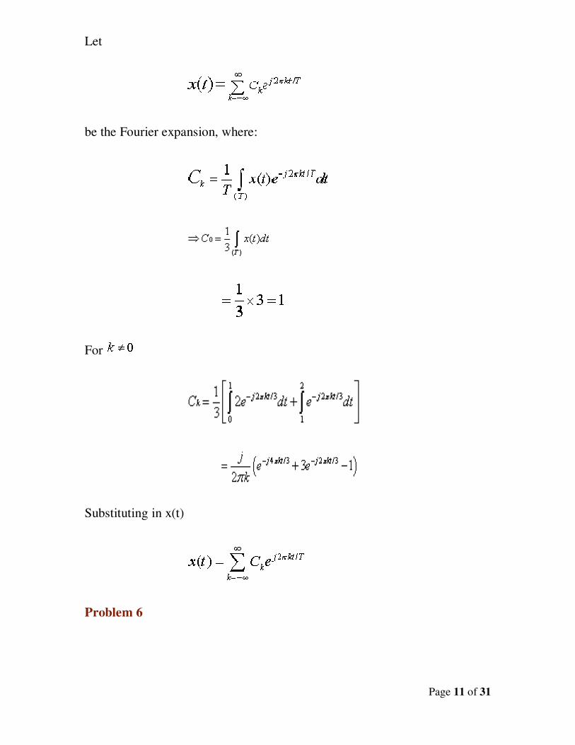
Let
be the Fourier expansion, where:
Page 5 of 31
For ,
But, in
Substituting in x(t)
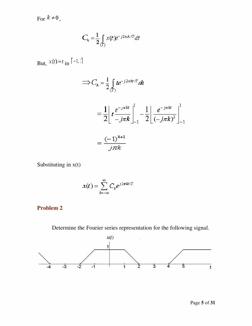
Problem 2
Determine the Fourier series representation for the following signal.
Page 6 of 31
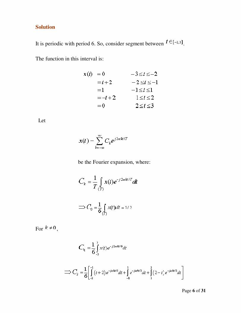
Solution
It is periodic with period 6. So, consider segment between .
The function in this interval is:
Let
be the Fourier expansion, where:
For ,
Page 7 of 31
Substituting in x(t)
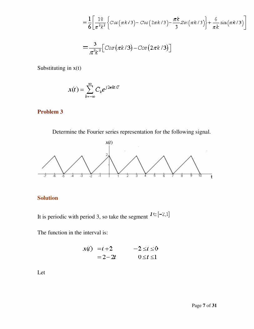
Problem 3
Determine the Fourier series representation for the following signal.
Solution
It is periodic with period 3, so take the segment
The function in the interval is:
Let
Page 8 of 31
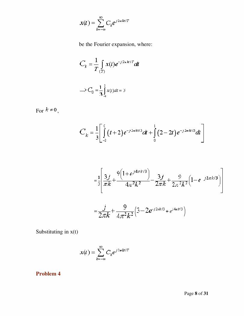
be the Fourier expansion, where:
For ,
Substituting in x(t)
Problem 4

Page 9 of 31
Determine the Fourier series representation for the following signal.
Solution
It is periodic with period 6. So, take the segment
Here will be
Let
be the Fourier expansion, where:
For
Page 10 of 31
Substituting in x(t)
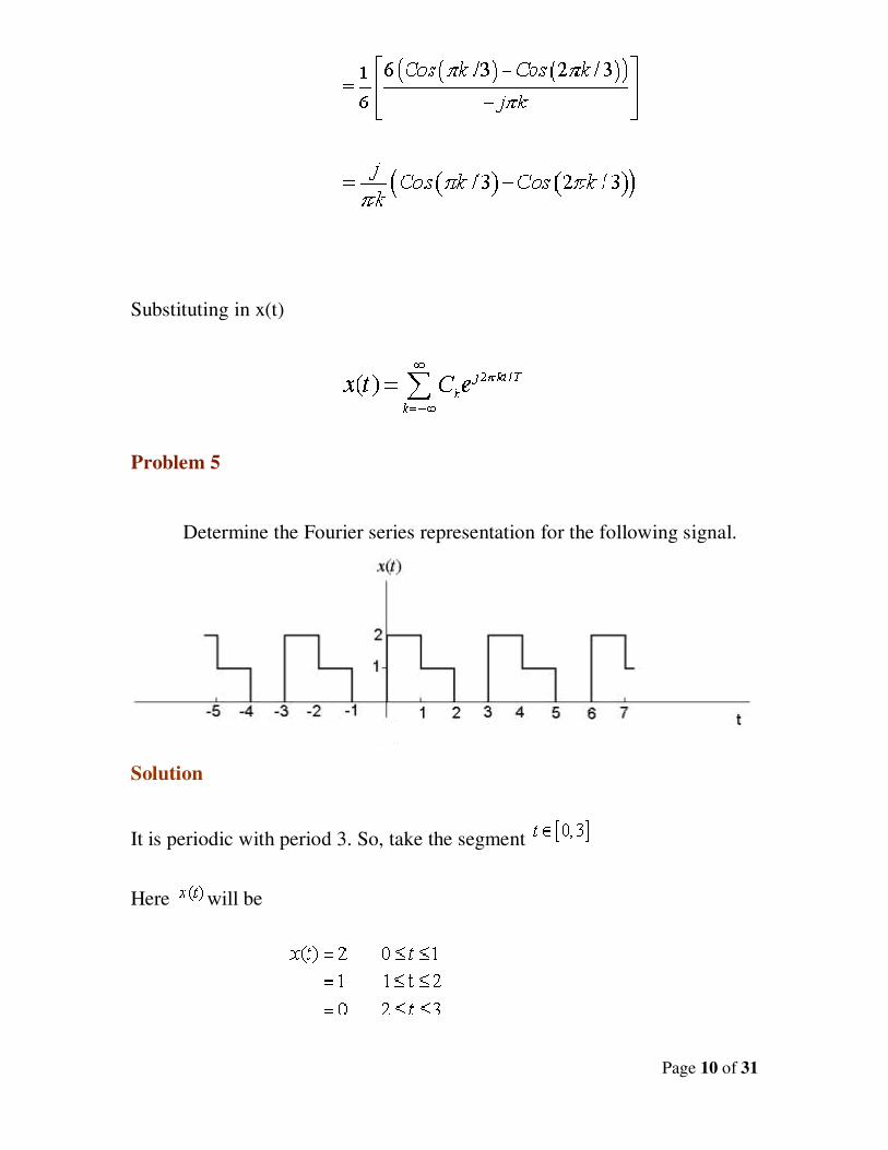
Problem 5
Determine the Fourier series representation for the following signal.
Solution
It is periodic with period 3. So, take the segment
Here will be
Page 11 of 31
Let
be the Fourier expansion, where:
For
Substituting in x(t)
Problem 6
Page 12 of 31
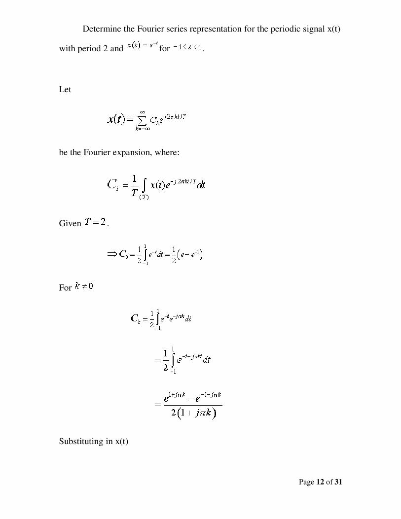
Determine the Fourier series representation for the periodic signal x(t)
with period 2 and for .
Let
be the Fourier expansion, where:
Given .
For
Substituting in x(t)
Page 13 of 31
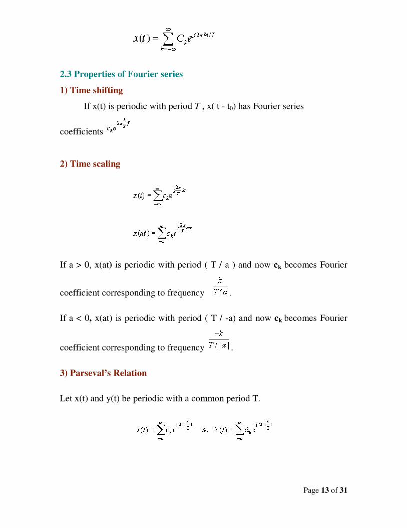
2.3 Properties of Fourier series
1) Time shifting
If x(t) is periodic with period T , x( t - t0) has Fourier series
coefficients
2) Time scaling
If a > 0, x(at) is periodic with period ( T / a ) and now ck becomes Fourier
coefficient corresponding to frequency .
If a < 0, x(at) is periodic with period ( T / -a) and now ck becomes Fourier
coefficient corresponding to frequency .
3) Parseval’s Relation
Let x(t) and y(t) be periodic with a common period T.
Page 14 of 31
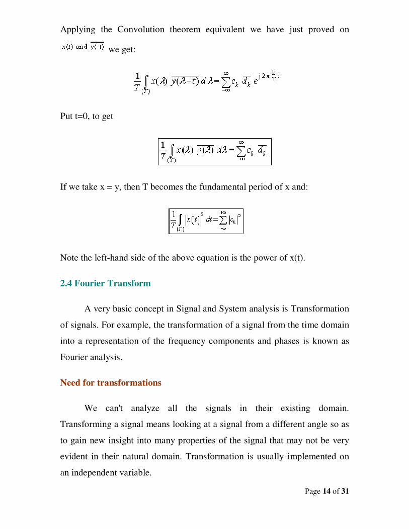
Applying the Convolution theorem equivalent we have just proved on
we get:
Put t=0, to get
If we take x = y, then T becomes the fundamental period of x and:
Note the left-hand side of the above equation is the power of x(t).
2.4 Fourier Transform
A very basic concept in Signal and System analysis is Transformation
of signals. For example, the transformation of a signal from the time domain
into a representation of the frequency components and phases is known as
Fourier analysis.
Need for transformations
We can't analyze all the signals in their existing domain.
Transforming a signal means looking at a signal from a different angle so as
to gain new insight into many properties of the signal that may not be very
evident in their natural domain. Transformation is usually implemented on
an independent variable.
Page 15 of 31
Every periodic signal can be written as a summation of sinusoidal
functions of frequencies which are multiples of a constant frequency (known
as fundamental frequency). This representation of a periodic signal is called
the Fourier series. An aperiodic signal can always be treated as a periodic
signal with an infinite period. The frequencies of two consecutive terms are
infinitesimally close and summation gets converted to integration. The
resulting pattern of this representation of an aperiodic signal is called the
Fourier Transform.
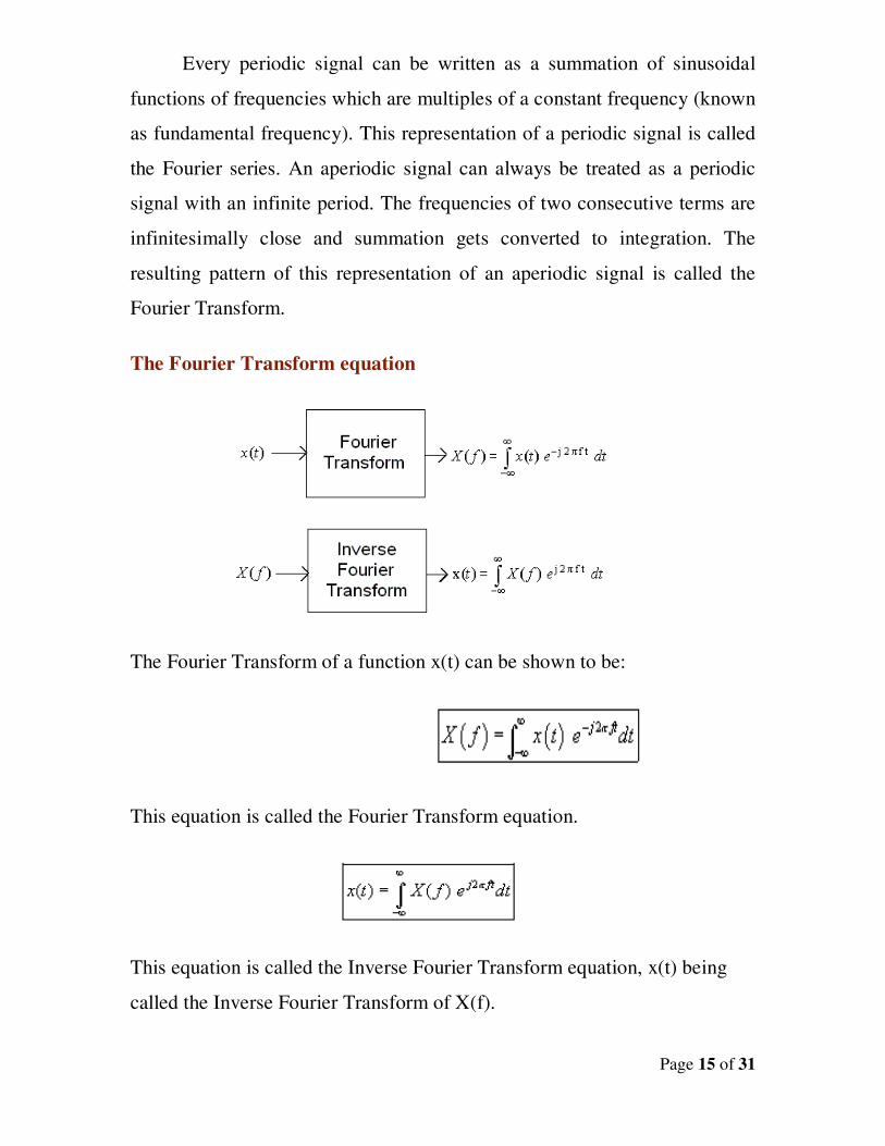
The Fourier Transform equation
The Fourier Transform of a function x(t) can be shown to be:
This equation is called the Fourier Transform equation.
This equation is called the Inverse Fourier Transform equation, x(t) being
called the Inverse Fourier Transform of X(f).
Page 16 of 31
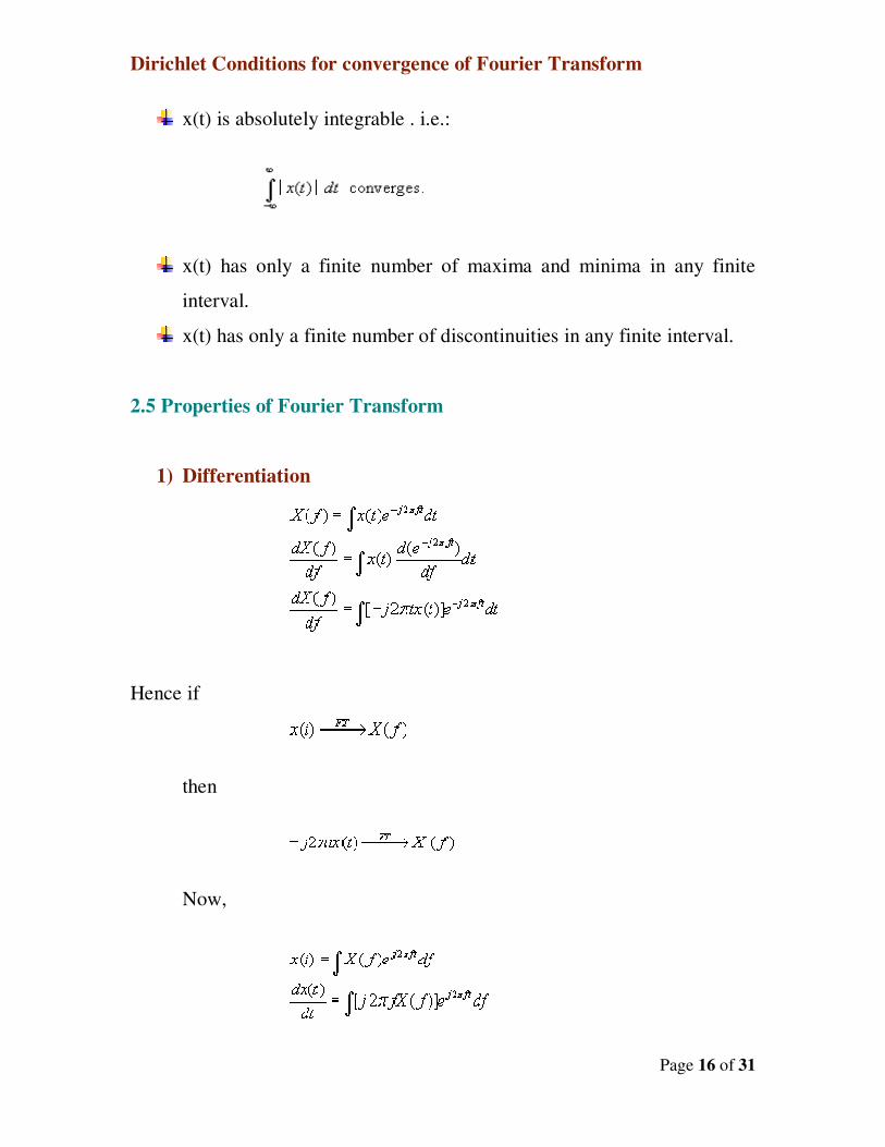
Dirichlet Conditions for convergence of Fourier Transform
x(t) is absolutely integrable . i.e.:
x(t) has only a finite number of maxima and minima in any finite
interval.
x(t) has only a finite number of discontinuities in any finite interval.
2.5 Properties of Fourier Transform
1) Differentiation
Hence if
then
Now,
Page 17 of 31
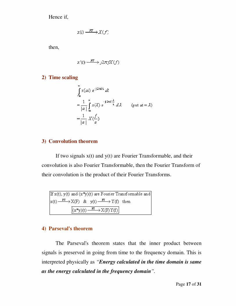
Hence if,
then,
2) Time scaling
3) Convolution theorem
If two signals x(t) and y(t) are Fourier Transformable, and their
convolution is also Fourier Transformable, then the Fourier Transform of
their convolution is the product of their Fourier Transforms.
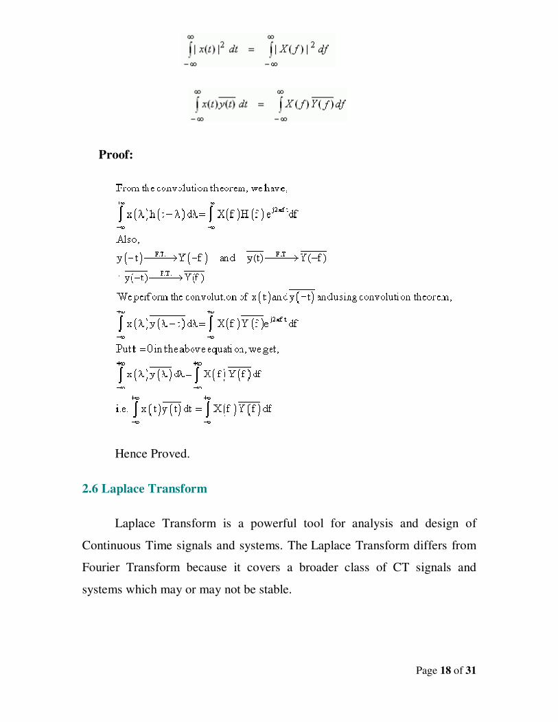
4) Parseval's theorem
The Parseval's theorem states that the inner product between
signals is preserved in going from time to the frequency domain. This is
interpreted physically as “Energy calculated in the time domain is same
as the energy calculated in the frequency domain”.
Page 18 of 31
Proof:
Hence Proved.
2.6 Laplace Transform
Laplace Transform is a powerful tool for analysis and design of
Continuous Time signals and systems. The Laplace Transform differs from
Fourier Transform because it covers a broader class of CT signals and
systems which may or may not be stable.
Page 19 of 31
Till now, we have seen the importance of Fourier analysis in solving
many problems involving signals. Now, we shall deal with signals which do
not have a Fourier transform.
We note that the Fourier Transform only exists for signals which can
absolutely integrated and have a finite energy. This observation leads to
generalization of continuous-time Fourier transform by considering a
broader class of signals using the powerful tool of "Laplace transform".
With this introduction let us go on to formally defining both Laplace
transform.
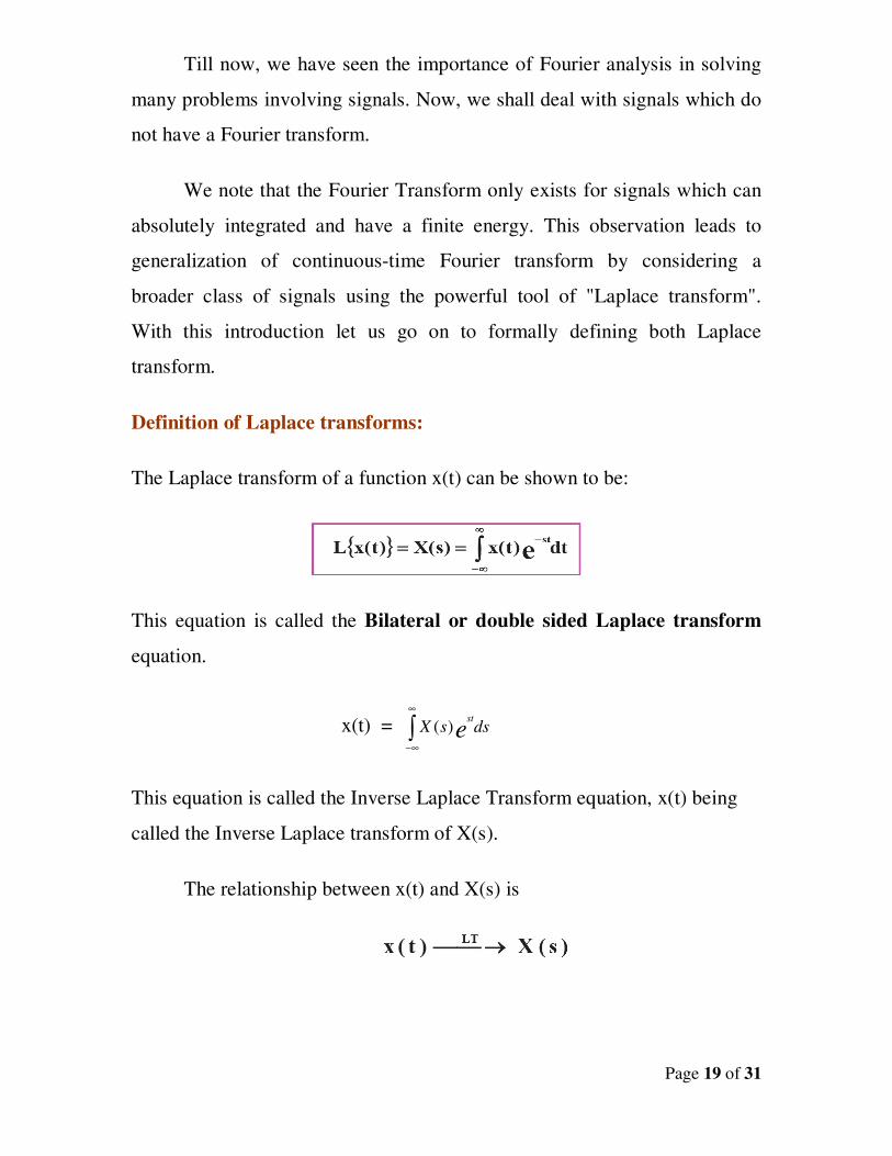
Definition of Laplace transforms:
The Laplace transform of a function x(t) can be shown to be:
This equation is called the Bilateral or double sided Laplace transform
equation.
x(t) = dssX est
∫∞
∞−
)(
This equation is called the Inverse Laplace Transform equation, x(t) being
called the Inverse Laplace transform of X(s).
The relationship between x(t) and X(s) is
Page 20 of 31
Region of Convergence (ROC):
The range of values for which the expression described above is finite
is called as the Region of Convergence (ROC).
Relationship between Laplace Transform and Fourier Transform
The Fourier Transform for Continuous Time signals is infact a special
case of Laplace Transform. This fact and subsequent relation between LT
and FT are explained below.
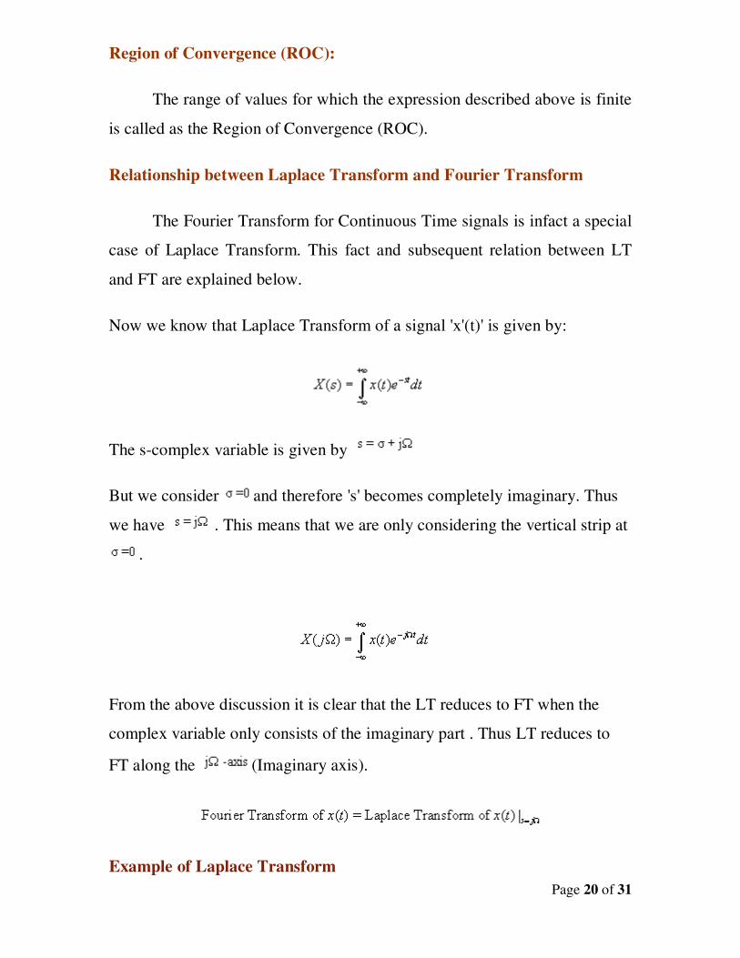
Now we know that Laplace Transform of a signal 'x'(t)' is given by:
The s-complex variable is given by
But we consider and therefore 's' becomes completely imaginary. Thus
we have . This means that we are only considering the vertical strip at
.
From the above discussion it is clear that the LT reduces to FT when the
complex variable only consists of the imaginary part . Thus LT reduces to
FT along the (Imaginary axis).
Example of Laplace Transform
Page 21 of 31
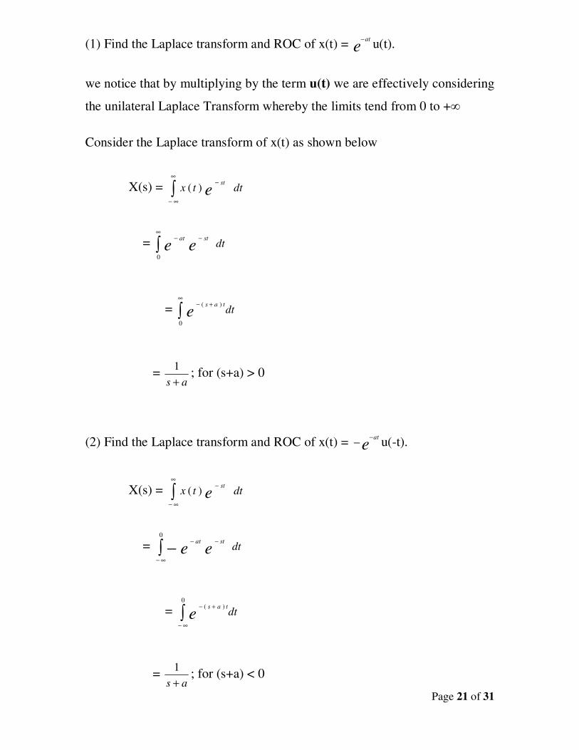
(1) Find the Laplace transform and ROC of x(t) = eat−
u(t).
we notice that by multiplying by the term u(t) we are effectively considering
the unilateral Laplace Transform whereby the limits tend from 0 to +∞
Consider the Laplace transform of x(t) as shown below
X(s) = dttx est
∫∞
∞−
−
)(
= dteestat
∫∞
−−
0
= dtetas
∫∞
+−
0
)(
= as +
1; for (s+a) > 0
(2) Find the Laplace transform and ROC of x(t) = eat−
− u(-t).
X(s) = dttx est
∫∞
∞−
−
)(
= dteestat
∫ −∞−
−−
0
= dtetas
∫∞−
+−
0)(
= as +
1; for (s+a) < 0

Page 22 of 31
If we consider the signals e-at
u(t) and -e-at
u(-t), we note that although
the signals are differing, their Laplace Transforms are identical which is
1/( s+a). Thus we conclude that to distinguish L.T's uniquely their ROC's
must be specified.
2.7 Properties of Laplace Transform
1) Linearity
If with ROC R1 and with ROC
R2, then with ROC containing
.
The ROC of X(s) is at least the intersection of R1 and R2, which
could be empty, in which case x(t) has no Laplace transform.
2) Differentiation in the time domain
If with ROC = R then with ROC =
R.
This property follows by integration-by-parts. Specifically let
Then,
Page 23 of 31
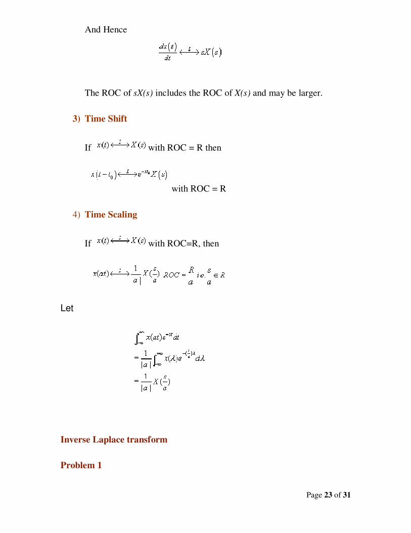
And Hence
The ROC of sX(s) includes the ROC of X(s) and may be larger.
3) Time Shift
If with ROC = R then
with ROC = R
4) Time Scaling
If with ROC=R, then
Let
Inverse Laplace transform
Problem 1

Page 24 of 31
Determine the function of time x (t), for the following Laplace Transform
and its associated regions of convergence:
Solution
Problem 2
Determine the function of time x (t), for the following Laplace Transform
and its associated regions of convergence:
Solution
Page 25 of 31
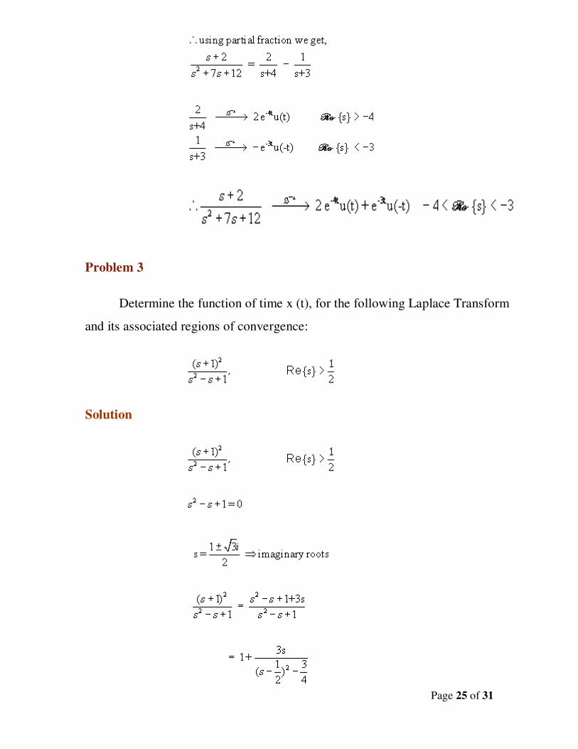
Problem 3
Determine the function of time x (t), for the following Laplace Transform
and its associated regions of convergence:
Solution
Page 26 of 31
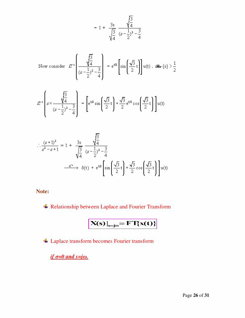
Note:
Relationship between Laplace and Fourier Transform
Laplace transform becomes Fourier transform
if σ=0 and s=jω.
Page 27 of 31
2.8 SAMPLING
Band-limited signals:
A Band-limited signal is one whose Fourier Transform is non-zero on
only a finite interval of the frequency axis.
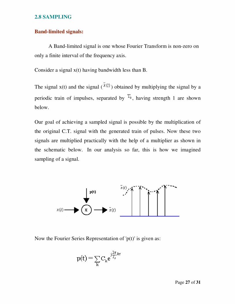
Consider a signal x(t) having bandwidth less than B.
The signal x(t) and the signal ( ) obtained by multiplying the signal by a
periodic train of impulses, separated by , having strength 1 are shown
below.
Our goal of achieving a sampled signal is possible by the multiplication of
the original C.T. signal with the generated train of pulses. Now these two
signals are multiplied practically with the help of a multiplier as shown in
the schematic below. In our analysis so far, this is how we imagined
sampling of a signal.
Now the Fourier Series Representation of 'p(t)' is given as:
Page 28 of 31
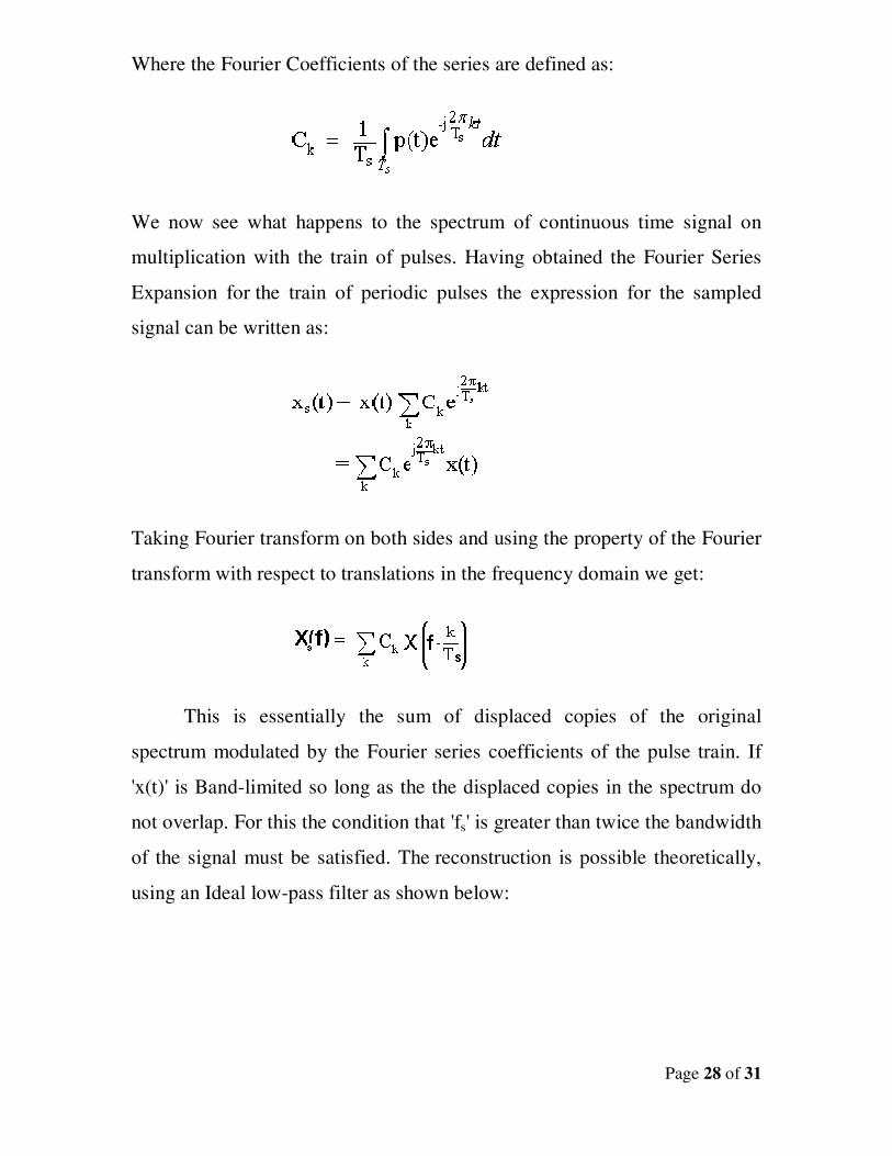
Where the Fourier Coefficients of the series are defined as:
We now see what happens to the spectrum of continuous time signal on
multiplication with the train of pulses. Having obtained the Fourier Series
Expansion for the train of periodic pulses the expression for the sampled
signal can be written as:
Taking Fourier transform on both sides and using the property of the Fourier
transform with respect to translations in the frequency domain we get:
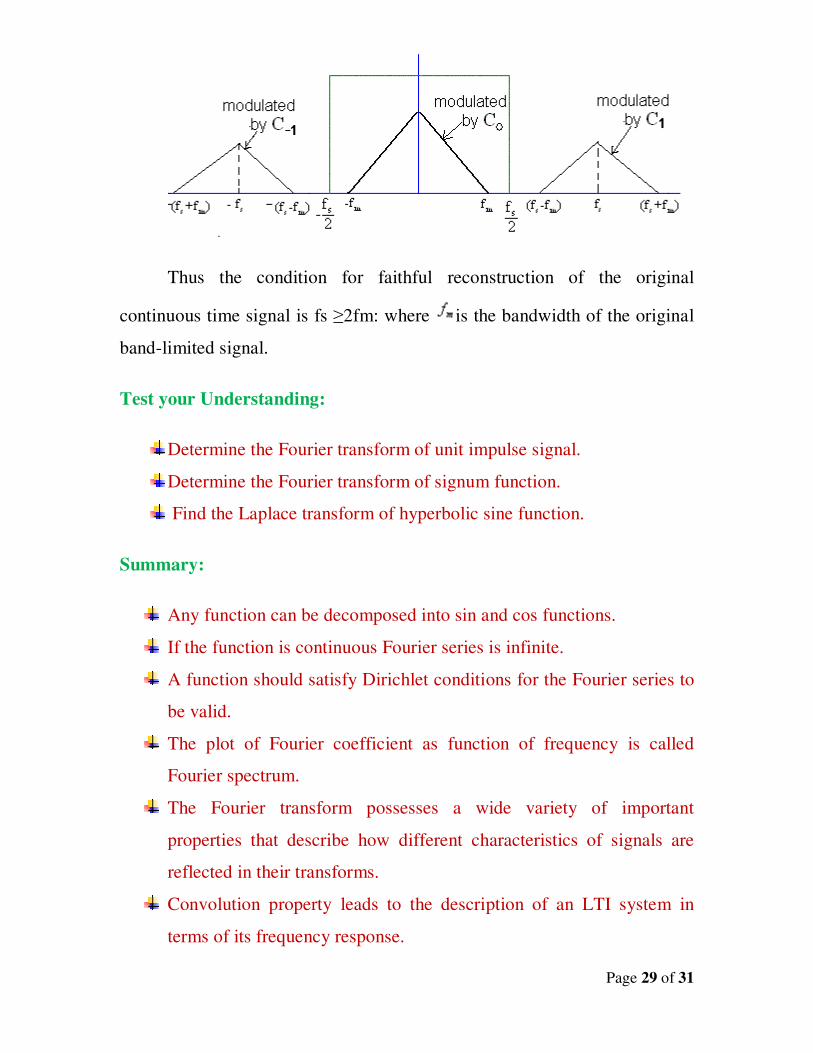
This is essentially the sum of displaced copies of the original
spectrum modulated by the Fourier series coefficients of the pulse train. If
'x(t)' is Band-limited so long as the the displaced copies in the spectrum do
not overlap. For this the condition that 'fs' is greater than twice the bandwidth
of the signal must be satisfied. The reconstruction is possible theoretically,
using an Ideal low-pass filter as shown below:
Page 29 of 31
Thus the condition for faithful reconstruction of the original
continuous time signal is fs ≥2fm: where is the bandwidth of the original
band-limited signal.
Test your Understanding:
Determine the Fourier transform of unit impulse signal.
Determine the Fourier transform of signum function.
Find the Laplace transform of hyperbolic sine function.
Summary:
Any function can be decomposed into sin and cos functions.
If the function is continuous Fourier series is infinite.
A function should satisfy Dirichlet conditions for the Fourier series to
be valid.
The plot of Fourier coefficient as function of frequency is called
Fourier spectrum.
The Fourier transform possesses a wide variety of important
properties that describe how different characteristics of signals are
reflected in their transforms.
Convolution property leads to the description of an LTI system in
terms of its frequency response.

Page 30 of 31
Two sided or bilateral Laplace Transform pair is defined as
The unilateral or single sided transform is defined as
We denote the transform from the time domain to frequency domain
and vice versa as
Review Questions:
What is Fourier series representation of a signal?
State Dirichlet’s conditions for convergence of Fourier series.
Write discrete time Fourier series pair.
List out the properties of Fourier series.
What is the need for transformation of signal?
Define Fourier Transform.
State Dirichlet’s conditions for convergence of Fourier Transform.
Define Laplace Transform.
Mention the properties of Laplace Transform.
What do you mean by sampling?
What is a band limited signal?
What are the criteria for sampling frequency to recover the original
signal?
Page 31 of 31
State Parseval’s theorem for discrete time signal.
Write the condition for the LTI system to be causal and stable.
Write synthesis and analysis equation of continuous time Fourier
series.
How do we fine Fourier series coefficient for a given signal.
State time shifting property of CT Fourier series.
State time shifting property of DT Fourier series.
Determine the Fourier series coefficient of sinωot.
State conjugate symmetry of CT Fourier series.
Determine the Fourier series coefficient of cosωon.